Adavnced Algorithms Lectures
Mathematical and Algorithmic FoundationsLinear Programming and Matchings
Paul G. Spirakis
Department of Computer ScienceUniversity of Patras and Liverpool
Paul G. Spirakis (U. Patras and Liverpool) Foundations -LP- Matcings 1 / 91

Outline
1 Linear programming
2 Bipartite matching
Paul G. Spirakis (U. Patras and Liverpool) Foundations -LP- Matcings 2 / 91
Linear programming Introduction
1 Linear programmingIntroductionThe geometry of LPFeasibility of LPDualitySolving a linear program
2 Bipartite matching
Paul G. Spirakis (U. Patras and Liverpool) Foundations -LP- Matcings 3 / 91
Linear programming Introduction
Linear programs
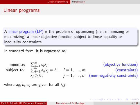
A linear program (LP) is the problem of optimizing (i.e., minimizing ormaximizing) a linear objective function subject to linear equality orinequality constraints.
In standard form, it is expressed as:
minimize∑n
j=1 cjxj (objective function)
subject to:∑n
j=1 aijxj = bi , i = 1, . . . ,m (constraints)
xj ≥ 0 , j = 1, . . . , n (non-negativity constraints)
where aij , bi , cj are given for all i , j .
Paul G. Spirakis (U. Patras and Liverpool) Foundations -LP- Matcings 4 / 91
Linear programming Introduction
Expressing LP using matrices
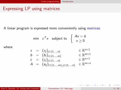
A linear program is expressed more conveniently using matrices:
min cT x subject to
{Ax = bx ≥ 0
wherex = (xj)j∈{1,...,n} ∈ Rn×1
b = (bi )i∈{1,...,m} ∈ Rm×1
c = (cj)j∈{1,...,n} ∈ Rn×1
A = (aij)i∈{1,...,m},j∈{1,...,n} ∈ Rm×n
Paul G. Spirakis (U. Patras and Liverpool) Foundations -LP- Matcings 5 / 91
Linear programming Introduction
Basic terminology
If x satisfies Ax = b, x ≥ 0, then x is feasible.
An LP is feasible if there exists a feasible solution, otherwise it is saidto be infeasible.
An optimal solution x∗ is a feasible solution such that
cT x∗ = min{cT x : Ax = b, x ≥ 0} .
An LP is unbounded (from below) if for all λ ∈ R, there exists afeasible x∗ such that
cT x∗ ≤ λ .
Paul G. Spirakis (U. Patras and Liverpool) Foundations -LP- Matcings 6 / 91
Linear programming Introduction
Equivalent forms
An LP can take several forms:
We might be maximizing instead of minimizing;
We might have a combination of equality and inequality constraints;
Some variables may be restricted to be non-positive instead ofnon-negative, or be unrestricted in sign.
Two forms are said to be equivalent if they have the same set of optimalsolutions or are both infeasible or both unbounded.
Paul G. Spirakis (U. Patras and Liverpool) Foundations -LP- Matcings 7 / 91
Linear programming Introduction
Equivalent forms
A maximization problem can be expressed as a minimization problem:
max cT x ⇔ min −cT x
An equality can be represented as a pair of inequalities:
aTi = bi ⇔{
aTi x ≤ biaTi x ≥ bi
⇔{
aTi x ≤ bi−aTi x ≤ −bi
By adding a slack variable, an inequality can be represented as acombination of equality and non-negativity constraints:
aTi x ≤ bi ⇔ aTi x + si = bi , si ≥ 0
Paul G. Spirakis (U. Patras and Liverpool) Foundations -LP- Matcings 8 / 91
Linear programming Introduction
Equivalent forms
Non-positivity constraints can be expressed as non-negativityconstraints: To express xj ≤ 0, replace xj everywhere with −yj andimpose the condition yj ≥ 0.
If xj is unrestricted in sign, i.e., non-positive or non-negative, replaceeverywhere xj by x+j − x−j , adding the constraints x+j , x
−j ≥ 0.
In general, an inequality can be represented using a combination ofequality and non-negativity constraints, and vice versa.
Paul G. Spirakis (U. Patras and Liverpool) Foundations -LP- Matcings 9 / 91
Linear programming Introduction
Canonical and standard forms
1 LP in canonical form:
min{cT x : Ax ≥ b}
2 LP in standard form:
min{cT x : Ax = b, x ≥ 0}
Using the rules described before, an LP in standard form may be written incanonical form, and vice versa.
Paul G. Spirakis (U. Patras and Liverpool) Foundations -LP- Matcings 10 / 91
Linear programming Introduction
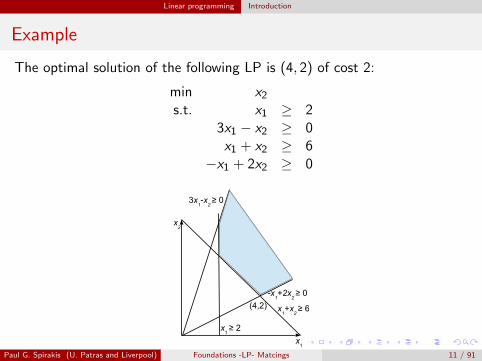
Example
The optimal solution of the following LP is (4, 2) of cost 2:
min x2s.t. x1 ≥ 2
3x1 − x2 ≥ 0x1 + x2 ≥ 6
−x1 + 2x2 ≥ 0
x2
x1
-x1+2x
2 ≥ 0
x1 ≥ 2
(4,2) x1+x
2 ≥ 6
3x1-x2 ≥ 0
Paul G. Spirakis (U. Patras and Liverpool) Foundations -LP- Matcings 11 / 91
Linear programming Introduction
Example
x2
x1
-x1+2x
2 ≥ 0
x1 ≥ 2
(4,2) x1+x
2 ≥ 6
3x1-x2 ≥ 0
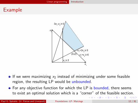
If we were maximizing x2 instead of minimizing under some feasibleregion, the resulting LP would be unbounded.
For any objective function for which the LP is bounded, there seemsto exist an optimal solution which is a “corner” of the feasible section.
Paul G. Spirakis (U. Patras and Liverpool) Foundations -LP- Matcings 12 / 91
Linear programming The geometry of LP
Vertices
Consider an LP in standard form:
min{cT x : Ax = b, x ≥ 0}
Let P = {x : Ax = b, x ≥ 0} ⊆ Rn.
Definition
x is a vertex of P if @y 6= 0 such that x + y ∈ P and x − y ∈ P.
Theorem
Assume min{cT x : x ∈ P} is finite. Then, for all x ∈ P, there exists avertex x ′ ∈ P such that
cT x ′ ≤ cT x .
Paul G. Spirakis (U. Patras and Liverpool) Foundations -LP- Matcings 13 / 91
Linear programming The geometry of LP
Vertices
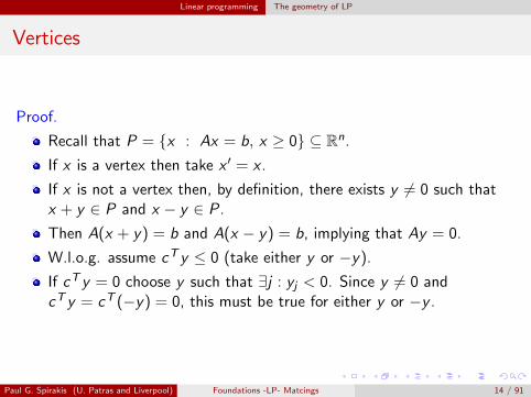
Proof.
Recall that P = {x : Ax = b, x ≥ 0} ⊆ Rn.
If x is a vertex then take x ′ = x .
If x is not a vertex then, by definition, there exists y 6= 0 such thatx + y ∈ P and x − y ∈ P.
Then A(x + y) = b and A(x − y) = b, implying that Ay = 0.
W.l.o.g. assume cT y ≤ 0 (take either y or −y).
If cT y = 0 choose y such that ∃j : yj < 0. Since y 6= 0 andcT y = cT (−y) = 0, this must be true for either y or −y .
Paul G. Spirakis (U. Patras and Liverpool) Foundations -LP- Matcings 14 / 91
Linear programming The geometry of LP
Vertices
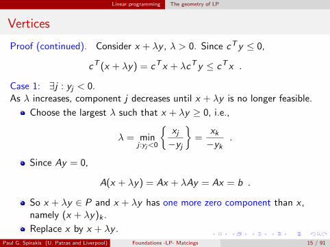
Proof (continued). Consider x + λy , λ > 0. Since cT y ≤ 0,
cT (x + λy) = cT x + λcT y ≤ cT x .
Case 1: ∃j : yj < 0.As λ increases, component j decreases until x + λy is no longer feasible.
Choose the largest λ such that x + λy ≥ 0, i.e.,
λ = minj :yj<0
{xj−yj
}=
xk−yk
.
Since Ay = 0,
A(x + λy) = Ax + λAy = Ax = b .
So x + λy ∈ P and x + λy has one more zero component than x ,namely (x + λy)k .
Replace x by x + λy .
Paul G. Spirakis (U. Patras and Liverpool) Foundations -LP- Matcings 15 / 91
Linear programming The geometry of LP
Vertices
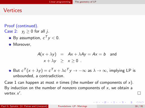
Proof (continued).Case 2: yj ≥ 0 for all j .
By assumption, cT y < 0.
Moreover,
A(x + λy) = Ax + λAy = Ax = b and
x + λy ≥ x ≥ 0 .
But cT (x + λy) = cT x + λcT y → −∞ as λ→∞, implying LP isunbounded, a contradiction.
Case 1 can happen at most n times (the number of components of x).By induction on the number of nonzero components of x , we obtain avertex x ′. �
Paul G. Spirakis (U. Patras and Liverpool) Foundations -LP- Matcings 16 / 91
Linear programming The geometry of LP
Vertices and optimal solutions
Corollary
If min{cT x : Ax = b, x ≥ 0} is finite, there exists an optimal solution x∗
which is a vertex.
Proof. Suppose not. Take an optimal solution.By the previous theorem, there exists a vertex costing no more than theoptimal. This vertex must be optimal as well! �
Corollary
If P = {x : Ax = b, x ≥ 0} 6= ∅ (i.e., if the LP is feasible), then P has avertex.
Paul G. Spirakis (U. Patras and Liverpool) Foundations -LP- Matcings 17 / 91
Linear programming The geometry of LP
A characterization of vertices
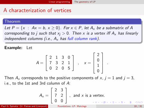
Theorem
Let P = {x : Ax = b, x ≥ 0}. For x ∈ P, let Ax be a submatrix of Acorresponding to j such that xj > 0. Then x is a vertex iff Ax has linearlyindependent columns (i.e., Ax has full column rank).
Example: Let
A =
2 1 3 07 3 2 10 2 0 5
, x =
2010
.
Then Ax corresponds to the positive components of x , j = 1 and j = 3,i.e., to the 1st and 3rd column of A:
Ax =
2 37 20 0
, and x is a vertex.
Paul G. Spirakis (U. Patras and Liverpool) Foundations -LP- Matcings 18 / 91
Linear programming The geometry of LP
A characterization of vertices
Proof (⇐).
Assume x is not a vertex. Then ∃y 6= 0 such that x + y , x − y ∈ P.
Since A(x + y) = b and A(x − y) = b, Ay = 0.
Let Ay be a submatrix of A corresponding to non-zero components ofy . Since y 6= 0 and Ay = 0, Ay has dependent columns.
x + y ≥ 0 and x − y ≥ 0 imply that yj = 0 whenever xj = 0.
Therefore Ay is a submatrix of Ax .
Therefore Ax has linearly dependent columns.
Paul G. Spirakis (U. Patras and Liverpool) Foundations -LP- Matcings 19 / 91
Linear programming The geometry of LP
A characterization of vertices
Proof (⇒).
Suppose Ax has linearly dependent columns. Then ∃y 6= 0 such thatAxy = 0.
Extend y to Rn by adding zero components.
Then ∃y ∈ Rn such that Ay = 0, y 6= 0, and yj = 0 whenever xj = 0.
Choose λ ≥ 0 such that x + λy , x − λy ≥ 0 andA(x + λy) = A(x − λy) = Ax = b.
So x + λy ∈ P and x − λy ∈ P.
Hence x is not a vertex.
�
Paul G. Spirakis (U. Patras and Liverpool) Foundations -LP- Matcings 20 / 91
Linear programming The geometry of LP
Basic feasible solutions
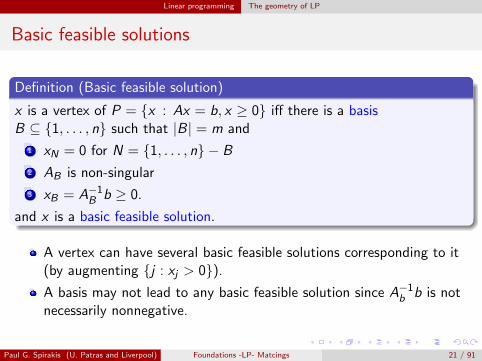
Definition (Basic feasible solution)
x is a vertex of P = {x : Ax = b, x ≥ 0} iff there is a basisB ⊆ {1, . . . , n} such that |B| = m and
1 xN = 0 for N = {1, . . . , n} − B
2 AB is non-singular
3 xB = A−1B b ≥ 0.
and x is a basic feasible solution.
A vertex can have several basic feasible solutions corresponding to it(by augmenting {j : xj > 0}).
A basis may not lead to any basic feasible solution since A−1b b is notnecessarily nonnegative.
Paul G. Spirakis (U. Patras and Liverpool) Foundations -LP- Matcings 21 / 91
Linear programming The geometry of LP
Basic feasible solutions
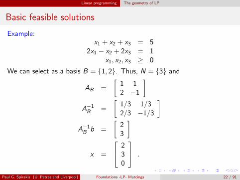
Example:x1 + x2 + x3 = 5
2x1 − x2 + 2x3 = 1x1, x2, x3 ≥ 0
We can select as a basis B = {1, 2}. Thus, N = {3} and
AB =
[1 12 −1
]A−1B =
[1/3 1/32/3 −1/3
]A−1B b =
[23
]
x =
230
.
Paul G. Spirakis (U. Patras and Liverpool) Foundations -LP- Matcings 22 / 91
Linear programming The geometry of LP
The Simplex method
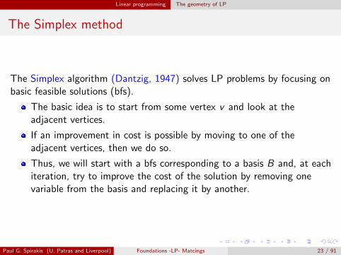
The Simplex algorithm (Dantzig, 1947) solves LP problems by focusing onbasic feasible solutions (bfs).
The basic idea is to start from some vertex v and look at theadjacent vertices.
If an improvement in cost is possible by moving to one of theadjacent vertices, then we do so.
Thus, we will start with a bfs corresponding to a basis B and, at eachiteration, try to improve the cost of the solution by removing onevariable from the basis and replacing it by another.
Paul G. Spirakis (U. Patras and Liverpool) Foundations -LP- Matcings 23 / 91
Linear programming The geometry of LP
The Simplex method
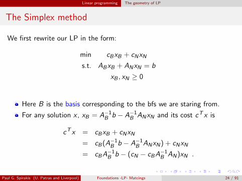
We first rewrite our LP in the form:
min cBxB + cNxN
s.t. ABxB + ANxN = b
xB , xN ≥ 0
Here B is the basis corresponding to the bfs we are staring from.
For any solution x , xB = A−1B b − A−1B ANxN and its cost cT x is
cT x = cBxB + cNxN
= cB(A−1B b − A−1B ANxN) + cNxN
= cBA−1B b − (cN − cBA
−1B AN)xN .
Paul G. Spirakis (U. Patras and Liverpool) Foundations -LP- Matcings 24 / 91
Linear programming The geometry of LP
The Simplex method
The cost of a solution x is cT x = cBA−1B b − (cN − cBA
−1B AN)xN .
We denote the reduced cost of the non-basic variables by cN :
cN = cN − cBA−1B AN ,
i.e., the quantity which is the coefficient of xN .
If there is a j ∈ N such that cj < 0, then by increasing xj (up fromzero) we will decrease the value of the objective function.
xB depends on xN , and we can increase xj only as long as all thecomponents of xB remain positive.
Paul G. Spirakis (U. Patras and Liverpool) Foundations -LP- Matcings 25 / 91
Linear programming The geometry of LP
The Simplex method
So, in a step of the Simplex method, we find a j ∈ N such thatcj < 0, and increase it as much as possible while keeping xB ≥ 0.
It is not possible any more to increase xj when one of the componentsof xB is zero.
What happened is that a non-basic variable is now positive and weinclude it in the basis, and one variable which was basic is now zero,so we remove it from the basis.
If there is no j ∈ N such that cj < 0, then we stop, and the currentbfs is optimal. This follows from the expression for cT x since xN isnonnegative.
Paul G. Spirakis (U. Patras and Liverpool) Foundations -LP- Matcings 26 / 91
Linear programming The geometry of LP
The Simplex method
Remark.Some of the basic variables may be zero to begin with, and we may not beable to increase xj at all.
We can replace j by k in the basis, but without moving from thevertex corresponding to the basis.
In the next step we might replace k by j , and be stuck in a loop.
Thus, we need to specify a pivoting rule to determine which indexshould enter the basis and which should be removed.
There is a pivoting rule which can not lead to infinite loops: choosethe minimal j and k possible.
There is no known pivoting rule for which the number of pivots in theworst case is better than exponential.
Paul G. Spirakis (U. Patras and Liverpool) Foundations -LP- Matcings 27 / 91
Linear programming The geometry of LP
The Simplex method
Complexity of the Simplex algorithm:
What is the length of the shortest path between two vertices of a convexpolyhedron, where the path is along edges, and the length of the path ismeasured in terms of the number of vertices visited?
Randomized pivoting: randomly permute the index columns of A andapply the Simplex method, always choosing the smallest j possible.
⇒ It is possible to show a subexponential bound on the expectednumber of pivots.
The question of the existence of a polynomial pivoting scheme isopen.
We will outline later a different algorithm which is polynomial: thatalgorithm will not move from one vertex to another, but will focus oninterior points of the feasible domain.
Paul G. Spirakis (U. Patras and Liverpool) Foundations -LP- Matcings 28 / 91
Linear programming Feasibility of LP
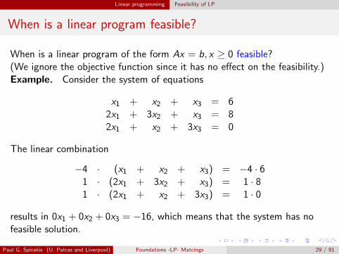
When is a linear program feasible?
When is a linear program of the form Ax = b, x ≥ 0 feasible?(We ignore the objective function since it has no effect on the feasibility.)Example. Consider the system of equations
x1 + x2 + x3 = 62x1 + 3x2 + x3 = 82x1 + x2 + 3x3 = 0
The linear combination
−4 · (x1 + x2 + x3) = −4 · 61 · (2x1 + 3x2 + x3) = 1 · 81 · (2x1 + x2 + 3x3) = 1 · 0
results in 0x1 + 0x2 + 0x3 = −16, which means that the system has nofeasible solution.
Paul G. Spirakis (U. Patras and Liverpool) Foundations -LP- Matcings 29 / 91
Linear programming Feasibility of LP
When is a linear program feasible?
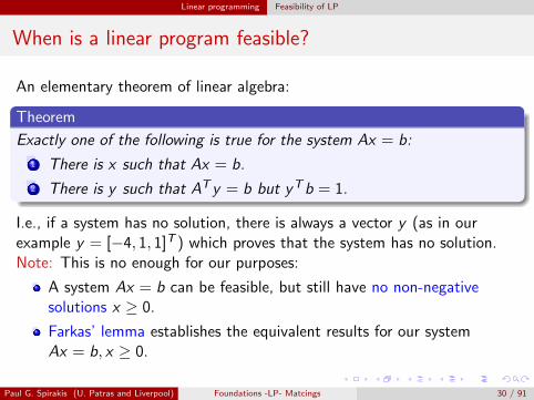
An elementary theorem of linear algebra:
Theorem
Exactly one of the following is true for the system Ax = b:
1 There is x such that Ax = b.
2 There is y such that AT y = b but yTb = 1.
I.e., if a system has no solution, there is always a vector y (as in ourexample y = [−4, 1, 1]T ) which proves that the system has no solution.Note: This is no enough for our purposes:
A system Ax = b can be feasible, but still have no non-negativesolutions x ≥ 0.
Farkas’ lemma establishes the equivalent results for our systemAx = b, x ≥ 0.
Paul G. Spirakis (U. Patras and Liverpool) Foundations -LP- Matcings 30 / 91
Linear programming Feasibility of LP
Farkas’ lemma
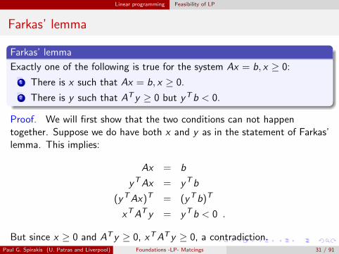
Farkas’ lemma
Exactly one of the following is true for the system Ax = b, x ≥ 0:
1 There is x such that Ax = b, x ≥ 0.
2 There is y such that AT y ≥ 0 but yTb < 0.
Proof. We will first show that the two conditions can not happentogether. Suppose we do have both x and y as in the statement of Farkas’lemma. This implies:
Ax = b
yTAx = yTb
(yTAx)T = (yTb)T
xTAT y = yTb < 0 .
But since x ≥ 0 and AT y ≥ 0, xTAT y ≥ 0, a contradiction.Paul G. Spirakis (U. Patras and Liverpool) Foundations -LP- Matcings 31 / 91
Linear programming Feasibility of LP
Farkas’ lemma
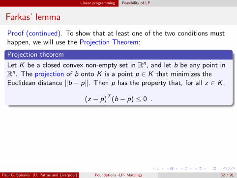
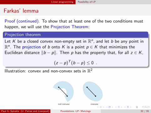
Proof (continued). To show that at least one of the two conditions musthappen, we will use the Projection Theorem:
Projection theorem
Let K be a closed convex non-empty set in Rn, and let b be any point inRn. The projection of b onto K is a point p ∈ K that minimizes theEuclidean distance ‖b − p‖. Then p has the property that, for all z ∈ K ,
(z − p)T (b − p) ≤ 0 .
Paul G. Spirakis (U. Patras and Liverpool) Foundations -LP- Matcings 32 / 91
Linear programming Feasibility of LP
Farkas’ lemma
Proof (continued). To show that at least one of the two conditions musthappen, we will use the Projection Theorem:
Projection theorem
Let K be a closed convex non-empty set in Rn, and let b be any point inRn. The projection of b onto K is a point p ∈ K that minimizes theEuclidean distance ‖b − p‖. Then p has the property that, for all z ∈ K ,
(z − p)T (b − p) ≤ 0 .
Illustration: convex and non-convex sets in R2
not convex convex
Paul G. Spirakis (U. Patras and Liverpool) Foundations -LP- Matcings 32 / 91
Linear programming Feasibility of LP
Farkas’ lemma
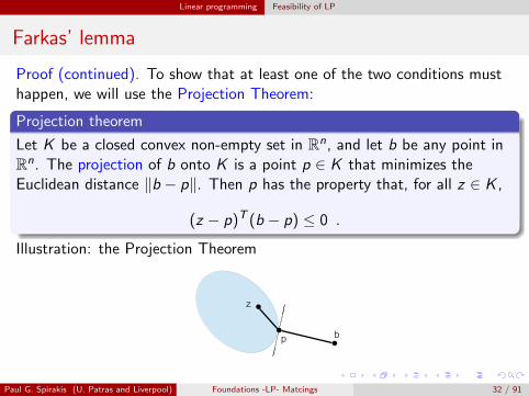
Proof (continued). To show that at least one of the two conditions musthappen, we will use the Projection Theorem:
Projection theorem
Let K be a closed convex non-empty set in Rn, and let b be any point inRn. The projection of b onto K is a point p ∈ K that minimizes theEuclidean distance ‖b − p‖. Then p has the property that, for all z ∈ K ,
(z − p)T (b − p) ≤ 0 .
Illustration: the Projection Theorem
z
p b
Paul G. Spirakis (U. Patras and Liverpool) Foundations -LP- Matcings 32 / 91
Linear programming Feasibility of LP
Farkas’ lemma
Proof (continued). Assume that there is no x such that Ax = b, x ≥ 0.We will show that there is y such that AT y ≥ 0 but yTb < 0.
Let K = {Ax : x ≥ 0} ⊆ Rm (A is an m × n matrix). K is a cone inRm, non-empty, convex, and closed.
Since Ax = b, x ≥ 0 has no solution, b /∈ K . Let p be the projectionof b onto K .
Since p ∈ K , there is a w ≥ 0 such that Aw = p.
According to the Projection Theorem, for all z ∈ K ,(z − p)T (b − p) ≤ 0. That is, for all x ≥ 0, (Ax − p)T (b − p) ≤ 0.
Define y = p − b, which implies (Ax − p)T y ≥ 0.
Since Aw = p, (Ax − Aw)T y ≥ 0 or (x − w)T (AT y) ≥ 0 for allx ≥ 0 (remember that w was fixed by choosing b).
Paul G. Spirakis (U. Patras and Liverpool) Foundations -LP- Matcings 33 / 91
Linear programming Feasibility of LP
Farkas’ lemma
Proof (continued).
Set x = w + [0 0 · · · 1 · · · 0]T (w plus a unit vector with a 1 in theith row). Note that x is non-negative, because w ≥ 0.
This will extract the ith column of A, so we conclude that the ithcomponent of AT y is non-negative, and since this is true for all i ,AT y ≥ 0.
It remains to show that yTb < 0. We have:
yTb = bT y = (p − y)T y = pT y − yT y .
Since (Ax − p)T y ≥ 0 for all x ≥ 0, taking x = 0 gives pT y ≤ 0.
Since b /∈ K , y = p − b 6= 0, so yT y > 0.
So yTb = pT y − yT y < 0. �
Paul G. Spirakis (U. Patras and Liverpool) Foundations -LP- Matcings 34 / 91
Linear programming Feasibility of LP
Farkas’ lemmaCanonical form
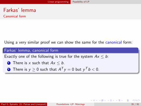
Using a very similar proof we can show the same for the canonical form:
Farkas’ lemma, canonical form
Exactly one of the following is true for the system Ax ≤ b:
1 There is x such that Ax ≤ b.
2 There is y ≥ 0 such that AT y = 0 but yTb < 0.
Paul G. Spirakis (U. Patras and Liverpool) Foundations -LP- Matcings 35 / 91
Linear programming Duality
The concept of duality
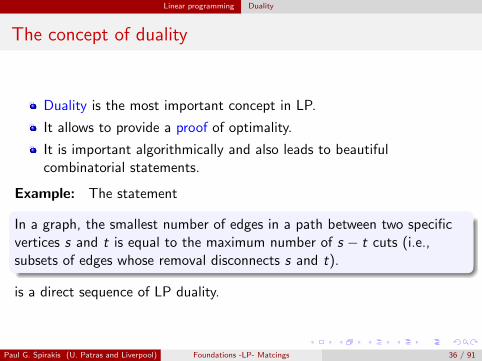
Duality is the most important concept in LP.
It allows to provide a proof of optimality.
It is important algorithmically and also leads to beautifulcombinatorial statements.
Example: The statement
In a graph, the smallest number of edges in a path between two specificvertices s and t is equal to the maximum number of s − t cuts (i.e.,subsets of edges whose removal disconnects s and t).
is a direct sequence of LP duality.
Paul G. Spirakis (U. Patras and Liverpool) Foundations -LP- Matcings 36 / 91
Linear programming Duality
Motivation of duality
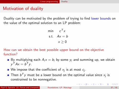
Duality can be motivated by the problem of trying to find lower bounds onthe value of the optimal solution to an LP problem:
min cT x
s.t. Ax = b
x ≥ 0
How can we obtain the best possible upper bound on the objectivefunction?
By multiplying each Aix = bi by some yi and summing up, we obtainyTAx = bT y .
We impose that the coefficient of xj is at most cj .
Then bT y must be a lower bound on the optimal value since xj isconstrained to be nonnegative.
Paul G. Spirakis (U. Patras and Liverpool) Foundations -LP- Matcings 37 / 91
Linear programming Duality
Motivation of duality
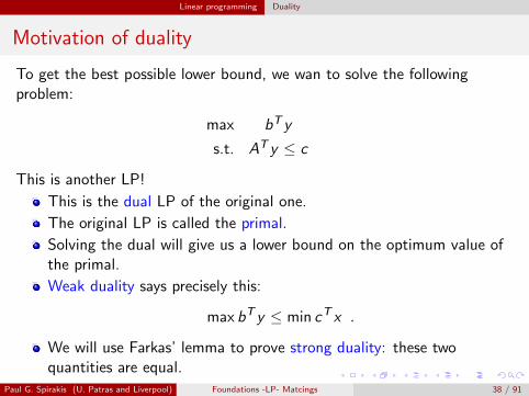
To get the best possible lower bound, we wan to solve the followingproblem:
max bT y
s.t. AT y ≤ c
This is another LP!
This is the dual LP of the original one.
The original LP is called the primal.
Solving the dual will give us a lower bound on the optimum value ofthe primal.
Weak duality says precisely this:
max bT y ≤ min cT x .
We will use Farkas’ lemma to prove strong duality: these twoquantities are equal.
Paul G. Spirakis (U. Patras and Liverpool) Foundations -LP- Matcings 38 / 91
Linear programming Duality
DualityExample
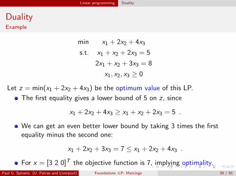
min x1 + 2x2 + 4x3
s.t. x1 + x2 + 2x3 = 5
2x1 + x2 + 3x3 = 8
x1, x2, x3 ≥ 0
Let z = min(x1 + 2x2 + 4x3) be the optimum value of this LP.
The first equality gives a lower bound of 5 on z , since
x1 + 2x2 + 4x3 ≥ x1 + x2 + 2x3 = 5 .
We can get an even better lower bound by taking 3 times the firstequality minus the second one:
x1 + 2x2 + 3x3 = 7 ≤ x1 + 2x2 + 4x3 .
For x = [3 2 0]T the objective function is 7, implying optimality.
Paul G. Spirakis (U. Patras and Liverpool) Foundations -LP- Matcings 39 / 91
Linear programming Duality
DualityExample
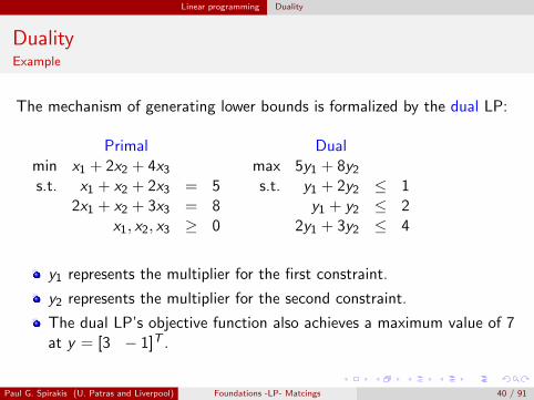
The mechanism of generating lower bounds is formalized by the dual LP:
Primal Dualmin x1 + 2x2 + 4x3s.t. x1 + x2 + 2x3 = 5
2x1 + x2 + 3x3 = 8x1, x2, x3 ≥ 0
max 5y1 + 8y2s.t. y1 + 2y2 ≤ 1
y1 + y2 ≤ 22y1 + 3y2 ≤ 4
y1 represents the multiplier for the first constraint.
y2 represents the multiplier for the second constraint.
The dual LP’s objective function also achieves a maximum value of 7at y = [3 − 1]T .
Paul G. Spirakis (U. Patras and Liverpool) Foundations -LP- Matcings 40 / 91
Linear programming Duality
DualityFormalization
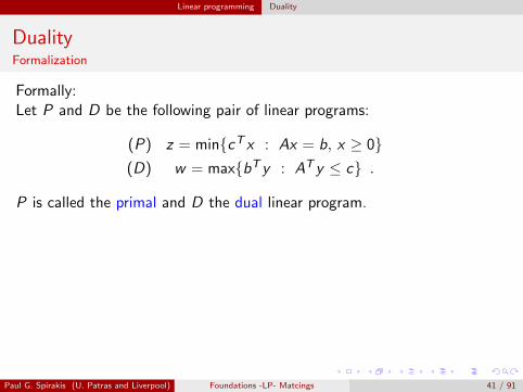
Formally:Let P and D be the following pair of linear programs:
(P) z = min{cT x : Ax = b, x ≥ 0}(D) w = max{bT y : AT y ≤ c} .
P is called the primal and D the dual linear program.
Claim
The dual of the dual is the primal.
I.e., if we formulate D as an LP in standard form (same as P), itsdual can be seen to be equivalent to the original primal P.
Thus, in any statement, we may replace the roles of primal and dualwithout affecting the statement.
Paul G. Spirakis (U. Patras and Liverpool) Foundations -LP- Matcings 41 / 91

Linear programming Duality
DualityFormalization
Formally:Let P and D be the following pair of linear programs:
(P) z = min{cT x : Ax = b, x ≥ 0}(D) w = max{bT y : AT y ≤ c} .
P is called the primal and D the dual linear program.
Claim
The dual of the dual is the primal.
I.e., if we formulate D as an LP in standard form (same as P), itsdual can be seen to be equivalent to the original primal P.
Thus, in any statement, we may replace the roles of primal and dualwithout affecting the statement.
Paul G. Spirakis (U. Patras and Liverpool) Foundations -LP- Matcings 41 / 91
Linear programming Duality
DualityThe dual of the dual is the primal
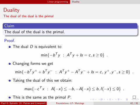
Claim
The dual of the dual is the primal.
Proof.
The dual D is equivalent to
min{−bT y : AT y + Is = c , s ≥ 0} .
Changing forms we get
min{−bT y+ + bT y− : AT y+ − AT y− + Is = c , y+, y−, s ≥ 0} .
Taking the dual of this we obtain:
max{−cT x : A(−x) ≤ −b,−A(−x) ≤ b, I (−x) ≤ 0} .
This is the same as the primal P. �Paul G. Spirakis (U. Patras and Liverpool) Foundations -LP- Matcings 42 / 91
Linear programming Duality
Weak duality
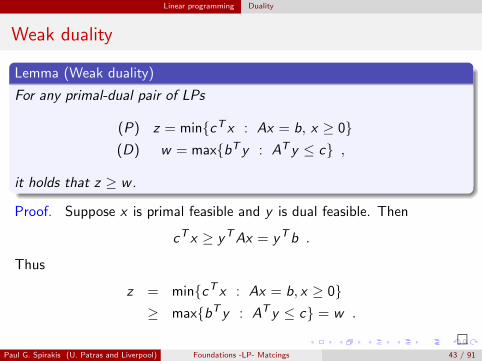
Lemma (Weak duality)
For any primal-dual pair of LPs
(P) z = min{cT x : Ax = b, x ≥ 0}(D) w = max{bT y : AT y ≤ c} ,
it holds that z ≥ w .
Proof. Suppose x is primal feasible and y is dual feasible. Then
cT x ≥ yTAx = yTb .
Thus
z = min{cT x : Ax = b, x ≥ 0}≥ max{bT y : AT y ≤ c} = w .
�Paul G. Spirakis (U. Patras and Liverpool) Foundations -LP- Matcings 43 / 91

Linear programming Duality
Strong duality
From weak duality we conclude that the following cases are not possible:
1 P is feasible and unbounded and D is feasible.
2 P is feasible and D is feasible and unbounded.
However, both the primal and the dual might be infeasible.
Stronger version of weak duality:
Theorem (Strong duality)
If P or D is feasible then z = w .
Paul G. Spirakis (U. Patras and Liverpool) Foundations -LP- Matcings 44 / 91
Linear programming Duality
Proof of strong duality
Proof. To prove strong duality, we recall the following corollary of Farkas’lemma:
Farkas’ lemma, canonical form
Exactly one of the following is true for the system A′x ′ ≤ b′:
1 There is x ′ such that A′x ′ ≤ b′.
2 There is y ′ ≥ 0 such that (A′)T y ′ = 0 and (b′)T y ′ < 0.
We only need to show that z ≤ w .
W.l.o.g. (by duality) assume P is feasible.
If P is unbounded, then by weak duality we have z = w = −∞.
Paul G. Spirakis (U. Patras and Liverpool) Foundations -LP- Matcings 45 / 91
Linear programming Duality
Proof of strong duality
Proof (continued).
If P is bounded, let x∗ be an optimal solution, i.e., Ax∗ = b, x∗ ≥ 0,and cT x∗ = z .
We claim that ∃y such that AT y ≤ c and bT y ≥ z . If so we are done.
Suppose no such y exists.
By Farkas’ lemma, with
A′ =
[AT
−bT], b′ =
[c−z
], x ′ = y , y ′ =
[xλ
],
there exist x ≥ 0, λ ≥ 0 such that Ax = λb and cT x < λz .
Paul G. Spirakis (U. Patras and Liverpool) Foundations -LP- Matcings 46 / 91
Linear programming Duality
Proof of strong duality
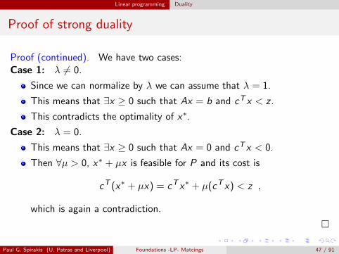
Proof (continued). We have two cases:Case 1: λ 6= 0.
Since we can normalize by λ we can assume that λ = 1.
This means that ∃x ≥ 0 such that Ax = b and cT x < z .
This contradicts the optimality of x∗.
Case 2: λ = 0.
This means that ∃x ≥ 0 such that Ax = 0 and cT x < 0.
Then ∀µ > 0, x∗ + µx is feasible for P and its cost is
cT (x∗ + µx) = cT x∗ + µ(cT x) < z ,
which is again a contradiction.
�
Paul G. Spirakis (U. Patras and Liverpool) Foundations -LP- Matcings 47 / 91
Linear programming Duality
Duality gap
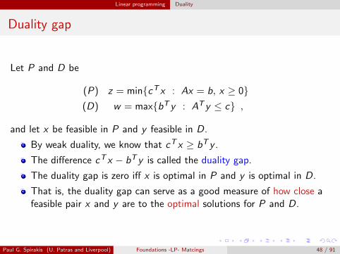
Let P and D be
(P) z = min{cT x : Ax = b, x ≥ 0}(D) w = max{bT y : AT y ≤ c} ,
and let x be feasible in P and y feasible in D.
By weak duality, we know that cT x ≥ bT y .
The difference cT x − bT y is called the duality gap.
The duality gap is zero iff x is optimal in P and y is optimal in D.
That is, the duality gap can serve as a good measure of how close afeasible pair x and y are to the optimal solutions for P and D.
Paul G. Spirakis (U. Patras and Liverpool) Foundations -LP- Matcings 48 / 91
Linear programming Duality
Duality gap
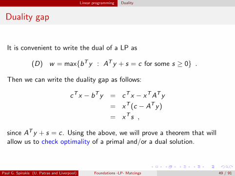
It is convenient to write the dual of a LP as
(D) w = max{bT y : AT y + s = c for some s ≥ 0} .
Then we can write the duality gap as follows:
cT x − bT y = cT x − xTAT y
= xT (c − AT y)
= xT s ,
since AT y + s = c . Using the above, we will prove a theorem that willallow us to check optimality of a primal and/or a dual solution.
Paul G. Spirakis (U. Patras and Liverpool) Foundations -LP- Matcings 49 / 91
Linear programming Duality
Complementary slackness
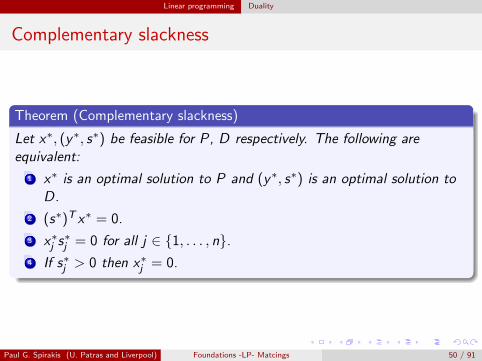
Theorem (Complementary slackness)
Let x∗, (y∗, s∗) be feasible for P, D respectively. The following areequivalent:
1 x∗ is an optimal solution to P and (y∗, s∗) is an optimal solution toD.
2 (s∗)T x∗ = 0.
3 x∗j s∗j = 0 for all j ∈ {1, . . . , n}.
4 If s∗j > 0 then x∗j = 0.
Paul G. Spirakis (U. Patras and Liverpool) Foundations -LP- Matcings 50 / 91
Linear programming Duality
Complementary slackness
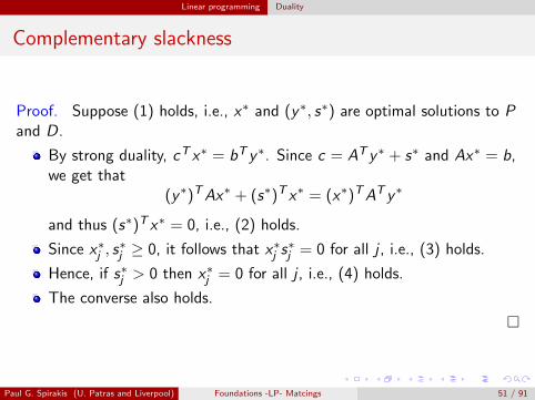
Proof. Suppose (1) holds, i.e., x∗ and (y∗, s∗) are optimal solutions to Pand D.
By strong duality, cT x∗ = bT y∗. Since c = AT y∗ + s∗ and Ax∗ = b,we get that
(y∗)TAx∗ + (s∗)T x∗ = (x∗)TAT y∗
and thus (s∗)T x∗ = 0, i.e., (2) holds.
Since x∗j , s∗j ≥ 0, it follows that x∗j s
∗j = 0 for all j , i.e., (3) holds.
Hence, if s∗j > 0 then x∗j = 0 for all j , i.e., (4) holds.
The converse also holds.
�
Paul G. Spirakis (U. Patras and Liverpool) Foundations -LP- Matcings 51 / 91
Linear programming Duality
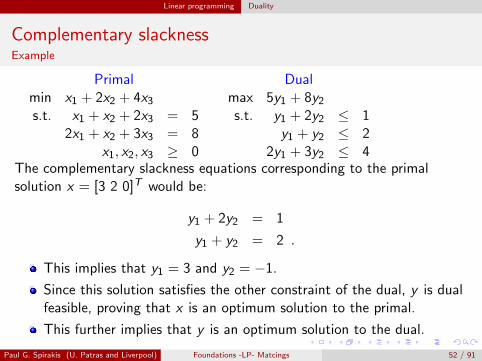
Complementary slacknessExample
Primal Dualmin x1 + 2x2 + 4x3s.t. x1 + x2 + 2x3 = 5
2x1 + x2 + 3x3 = 8x1, x2, x3 ≥ 0
max 5y1 + 8y2s.t. y1 + 2y2 ≤ 1
y1 + y2 ≤ 22y1 + 3y2 ≤ 4
The complementary slackness equations corresponding to the primalsolution x = [3 2 0]T would be:
y1 + 2y2 = 1
y1 + y2 = 2 .
This implies that y1 = 3 and y2 = −1.
Since this solution satisfies the other constraint of the dual, y is dualfeasible, proving that x is an optimum solution to the primal.
This further implies that y is an optimum solution to the dual.
Paul G. Spirakis (U. Patras and Liverpool) Foundations -LP- Matcings 52 / 91
Linear programming Solving a linear program
Complexity of linear programming
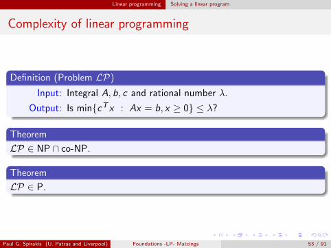
Definition (Problem LP)
Input: Integral A, b, c and rational number λ.
Output: Is min{cT x : Ax = b, x ≥ 0} ≤ λ?
Theorem
LP ∈ NP ∩ co-NP.
Theorem
LP ∈ P.
Paul G. Spirakis (U. Patras and Liverpool) Foundations -LP- Matcings 53 / 91
Linear programming Solving a linear program
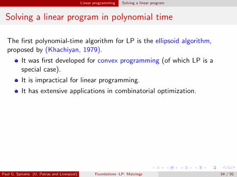
Solving a linear program in polynomial time
The first polynomial-time algorithm for LP is the ellipsoid algorithm,proposed by (Khachiyan, 1979).
It was first developed for convex programming (of which LP is aspecial case).
It is impractical for linear programming.
It has extensive applications in combinatorial optimization.
(Karmarkar, 1984) presented another polynomial-time algorithm for LP.
It avoids the combinatorial complexity (inherent in the simplexalgorithm) of the vertices of the polyhedron by staying well inside thepolyhedron.
It lead to many other algorithms for LP based on similar ideas.
These algorithms are known as interior point methods.
Paul G. Spirakis (U. Patras and Liverpool) Foundations -LP- Matcings 54 / 91
Linear programming Solving a linear program
Solving a linear program in polynomial time
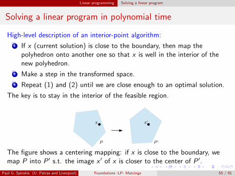
High-level description of an interior-point algorithm:
1 If x (current solution) is close to the boundary, then map thepolyhedron onto another one so that x is well in the interior of thenew polyhedron.
2 Make a step in the transformed space.
3 Repeat (1) and (2) until we are close enough to an optimal solution.
The key is to stay in the interior of the feasible region.
x'x
P P'
The figure shows a centering mapping: if x is close to the boundary, wemap P into P ′ s.t. the image x ′ of x is closer to the center of P ′.
Paul G. Spirakis (U. Patras and Liverpool) Foundations -LP- Matcings 55 / 91
Bipartite matching
1 Linear programming
2 Bipartite matchingBipartite graphs and matchingsMaximum cardinality matchingMinimum weight perfect matching
Paul G. Spirakis (U. Patras and Liverpool) Foundations -LP- Matcings 56 / 91
Bipartite matching Bipartite graphs and matchings
Bipartite graphs
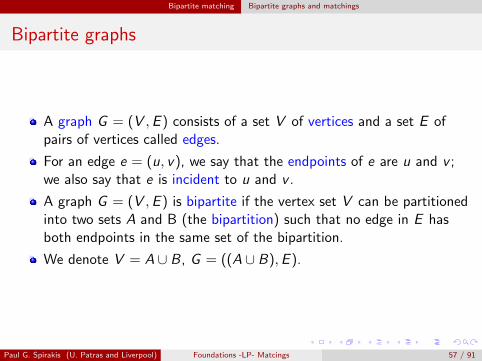
A graph G = (V ,E ) consists of a set V of vertices and a set E ofpairs of vertices called edges.
For an edge e = (u, v), we say that the endpoints of e are u and v ;we also say that e is incident to u and v .
A graph G = (V ,E ) is bipartite if the vertex set V can be partitionedinto two sets A and B (the bipartition) such that no edge in E hasboth endpoints in the same set of the bipartition.
We denote V = A ∪ B, G = ((A ∪ B),E ).
Paul G. Spirakis (U. Patras and Liverpool) Foundations -LP- Matcings 57 / 91
Bipartite matching Bipartite graphs and matchings
Matchings
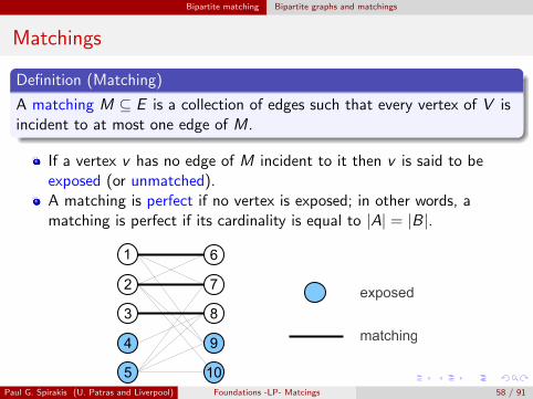
Definition (Matching)
A matching M ⊆ E is a collection of edges such that every vertex of V isincident to at most one edge of M.
If a vertex v has no edge of M incident to it then v is said to beexposed (or unmatched).A matching is perfect if no vertex is exposed; in other words, amatching is perfect if its cardinality is equal to |A| = |B|.
2
3
4
5
6
7
8
9
10
1
exposed
matching
Paul G. Spirakis (U. Patras and Liverpool) Foundations -LP- Matcings 58 / 91
Bipartite matching Bipartite graphs and matchings
Matching problems
We are interested in the following two problems on bipartite graphs:
Maximum cardinality matching problem
Find a matching M of maximum size.
Minimum weight perfect matching problem
Given a cost cij for all (i , j) ∈ A× B, find a perfect matching of minimumcost where the cost of a matching M is given by
c(M) =∑
(i ,j)∈M
cij .
This problem is also called the assignment problem.
Note that similar problems (but more complicated) can be defined onnon-bipartite graphs.
Paul G. Spirakis (U. Patras and Liverpool) Foundations -LP- Matcings 59 / 91
Bipartite matching Maximum cardinality matching
Optimality of a matching
Before describing an algorithm for solving the maximum cardinalitymatching problem, one would like to be able to prove optimality of amatching (without reference to any algorithm).
For this purpose, one would like to find upper bounds on the size ofany matching and hope that the smallest of these upper bounds beequal to the size of the largest matching.
This is a duality concept that will be ubiquitous in this subject.
Paul G. Spirakis (U. Patras and Liverpool) Foundations -LP- Matcings 60 / 91
Bipartite matching Maximum cardinality matching
Konig’s theorem
A vertex cover is a subset C of vertices such that all edges e ∈ E areincident to at least one vertex of C . In other words, there is no edgecompletely contained in V \ C .
Clearly, the size of any matching is at most the size of any vertexcover: given any matching M, a vertex cover C must contain at leastone of the endpoints of each edge in M.
We have just proved weak duality: that the maximum size of amatching is at most the minimum size of a vertex cover. We willprove that equality in fact holds:
Theorem (Konig’s theorem)
For any bipartite graph, the maximum size of a matching is equal to theminimum size of a vertex cover.
Paul G. Spirakis (U. Patras and Liverpool) Foundations -LP- Matcings 61 / 91
Bipartite matching Maximum cardinality matching
Konig’s theorem
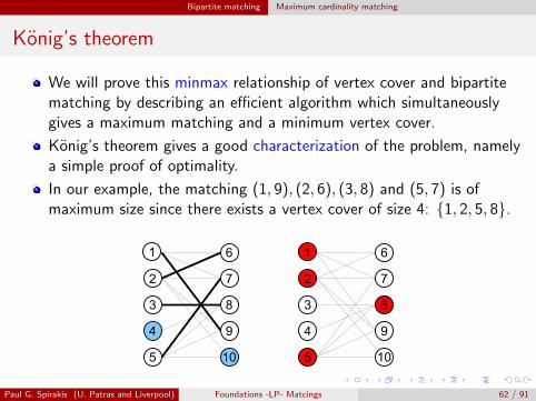
We will prove this minmax relationship of vertex cover and bipartitematching by describing an efficient algorithm which simultaneouslygives a maximum matching and a minimum vertex cover.
Konig’s theorem gives a good characterization of the problem, namelya simple proof of optimality.
In our example, the matching (1, 9), (2, 6), (3, 8) and (5, 7) is ofmaximum size since there exists a vertex cover of size 4: {1, 2, 5, 8}.
2
3
4
5
6
7
8
9
10
1
2
3
4
5
6
7
8
9
10
1
Paul G. Spirakis (U. Patras and Liverpool) Foundations -LP- Matcings 62 / 91
Bipartite matching Maximum cardinality matching
Solving the cardinality matching problem
The natural approach to solving this cardinality matching problem isto try a greedy algorithm: Start with any matching (e.g. an emptymatching) and repeatedly add disjoint edges until no more edges canbe added.
This approach, however, is not guaranteed to give a maximummatching.
We will present an algorithm that does work, and is based on theconcepts of alternating paths and augmenting paths.
Paul G. Spirakis (U. Patras and Liverpool) Foundations -LP- Matcings 63 / 91
Bipartite matching Maximum cardinality matching
Alternating and augmenting paths
A path is simply a collection of edges (v0, v1), (v1, v2), . . . , (vk−1, vk)where the vi ’s are distinct vertices. A path can simply be representedas v0 − v1 − vk .
An alternating path with respect to M is a path that alternatesbetween edges in M and edges in E \M.
An augmenting path with respect to M is an alternating path inwhich the first and last vertices are exposed.
Paul G. Spirakis (U. Patras and Liverpool) Foundations -LP- Matcings 64 / 91
Bipartite matching Maximum cardinality matching
Alternating and augmenting pathsProperties
Some properties of augmenting paths:
An augmenting path with respect to M which contains k edges of Mmust also contain exactly k + 1 edges not in M.
The two endpoints of an augmenting path must be on different sidesof the bipartition.
The most interesting property of an augmenting path P with respect to amatching M is that
If we set M ′ = (M \ P) ∪ (P \M), then we get a matching M ′ and,moreover, the size of M ′ is one unit larger than the size of M.
This means that we can form a larger matching M ′ from M by takingthe edges of P not in M and adding them to M ′ while removing fromM ′ the edges in M that are also in the path P.
We say that we have augmented M along P.
Paul G. Spirakis (U. Patras and Liverpool) Foundations -LP- Matcings 65 / 91
Bipartite matching Maximum cardinality matching
Alternating and augmenting pathsUsefulness
The usefulness of augmenting paths is given in the following theorem.
Theorem
A matching M is maximum if and only if there are no augmenting pathswith respect to M.
Proof:(⇒) By contradiction:
Let P be some augmenting path with respect to M.
Set M ′ = (M \ P) ∪ (P \M).
Then M ′ is a matching with cardinality greater than M.
This contradicts the maximality of M.
Paul G. Spirakis (U. Patras and Liverpool) Foundations -LP- Matcings 66 / 91
Bipartite matching Maximum cardinality matching
Alternating and augmenting pathsUsefulness
Proof (continued):(⇐) Again by contradiction: If M is not maximum, let M∗ be a maximummatching (so that |M∗| > |M|). Let Q = (M \M∗) ∪ (M∗ \M). Then:
Q has more edges from M∗ than from M (since |M∗| > |M| implies|M∗ \M| > |M \M∗|).
Each vertex is incident to at most one edge in M ∩ Q and one edgeM∗ ∩ Q.
Thus Q is composed of cycles and paths that alternate between edgesfrom M and M∗.
Therefore there must be some path with more edges from M∗ in itthan from M (all cycles will be of even length and have the samenumber of edges from M∗ and M). This path is an augmenting pathwith respect to M.
Hence there must exist an augmenting path P with respect to M,which is a contradiction. �
Paul G. Spirakis (U. Patras and Liverpool) Foundations -LP- Matcings 67 / 91
Bipartite matching Maximum cardinality matching
An algorithm for maximum cardinality matching
The theorem we just proved, i.e.,
A matching M is maximum if and only if there are no augmenting pathswith respect to M.
motivates the following algorithm.
1 Start with any matching M, say the empty matching.
2 Repeatedly locate an augmenting path P with respect to M, augmentM along P and replace M by the resulting matching.
3 Stop when no more augmenting path exists.
By the above theorem, we are guaranteed to have found an optimummatching.The algorithm terminates in µ augmentations, where µ is the size ofthe maximum matching.Clearly, µ ≤ n
2 , where n = |V |.Paul G. Spirakis (U. Patras and Liverpool) Foundations -LP- Matcings 68 / 91
Bipartite matching Maximum cardinality matching
An algorithm for maximum cardinality matching
The question now is how to decide the existence of an augmenting pathand how to find one, if one exists.These tasks can be done as follows: Direct edges in G according to M sothat
an edge goes from A to B if it does not belong to the matching Mand
an edge goes from B to A if it does.
Call this directed graph D.
Lemma
There exists an augmenting path in G with respect to M iff there exists adirected path in D between an exposed vertex in A and an exposed vertexin B.
Paul G. Spirakis (U. Patras and Liverpool) Foundations -LP- Matcings 69 / 91
Bipartite matching Maximum cardinality matching
An algorithm for maximum cardinality matching
This gives an O(m) algorithm (where m = |E |) for finding anaugmenting path in G .
Let A∗ and B∗ be the set of exposed vertices w.r.t. M in A and Brespectively.
We can simply attach a vertex s to all the vertices in A∗ and do adepth-first-search from s till we hit a vertex in B∗ and then traceback our path.
Thus the overall complexity of finding a maximum cardinalitymatching is O(nm).
This can be improved to O(√nm) by augmenting along several
augmenting paths simultaneously.
Paul G. Spirakis (U. Patras and Liverpool) Foundations -LP- Matcings 70 / 91
Bipartite matching Maximum cardinality matching
An algorithm for maximum cardinality matching
If there is no augmenting path w.r.t. M, then we can also use oursearch procedure for an augmenting path in order to construct anoptimum vertex cover.
Consider the set L of vertices which can be reached by a directedpath from an exposed vertex in A.
The following claim immediately proves Konig’s theorem.
Claim
When the algorithm terminates, C ∗ = (A− L) ∪ (B ∩ L) is a vertex cover.Moreover, |C ∗| = |M∗| where M∗ is the matching returned by thealgorithm.
Paul G. Spirakis (U. Patras and Liverpool) Foundations -LP- Matcings 71 / 91
Bipartite matching Maximum cardinality matching
An algorithm for maximum cardinality matching
Proof. We first show that C ∗ is a vertex cover.
Assume not. Then there must exist an edge e = (a, b) ∈ E witha ∈ A ∩ L and b ∈ (B − L).
Edge e cannot belong to the matching. If it did, then b should be inL for otherwise a would not be in L.
Hence, e must be in E −M and is therefore directed from A to B.
This implies that b can be reached from an exposed vertex in A(namely go to a and then take the edge (a, b)), contradicting the factthat b /∈ L.
Paul G. Spirakis (U. Patras and Liverpool) Foundations -LP- Matcings 72 / 91
Bipartite matching Maximum cardinality matching
An algorithm for maximum cardinality matching
Proof (continued). To show that |C ∗| = |M∗|, we show that |C ∗| ≤ |M∗|,since the reverse inequality is true for any matching and any vertex cover.Observations:
1 No vertex in A− L is exposed by definition of L.
2 No vertex in B ∩ L is exposed since this would imply the existence ofan augmenting path and, thus, the algorithm would not haveterminated.
3 There is no edge of the matching between a vertex a ∈ (A− L) and avertex b ∈ (B ∩ L). Otherwise, a would be in L.
These remarks imply that every vertex in C ∗ is matched and moreover thecorresponding edges of the matching are distinct. Hence, |C ∗| ≤ |M∗|. �
Paul G. Spirakis (U. Patras and Liverpool) Foundations -LP- Matcings 73 / 91
Bipartite matching Maximum cardinality matching
Hall’s theorem
Hall’s theorem gives a necessary and sufficient condition for a bipartitegraph to have a matching which saturates (or matches) all vertices of A(i.e., a matching of size |A|).
Theorem (Hall, 1935)
Given a bipartite graph G = (V ,E ) with bipartition A,B (V = A ∪ B), Ghas a matching of size |A| if and only if, for every S ⊆ A, we have|N(S)| ≥ |S |, where N(S) = {b ∈ B : ∃a ∈ S with (a, b) ∈ E}.
Clearly, the condition given in Hall’s theorem is necessary.
Its sufficiency can be derived from Konig’s theorem.
Paul G. Spirakis (U. Patras and Liverpool) Foundations -LP- Matcings 74 / 91
Bipartite matching Minimum weight perfect matching
Minimum weighted perfect matching problem
By assigning infinite costs to the edges not present, one can assumethat the bipartite graph G = ((A ∪ B),E ) is complete, i.e.,E = A× B.
The minimum weight perfect matching problem is often described bythe following story:
There are n jobs to be processed on n machines and one would like toprocess exactly one job per machine such that the total cost of processingthe jobs is minimized.
Formally, we are given costs cij ∈ R ∪ {∞} for every i ∈ A, j ∈ B and thegoal is to find a perfect matching M minimizing
∑(i ,j)∈M cij .
Paul G. Spirakis (U. Patras and Liverpool) Foundations -LP- Matcings 75 / 91
Bipartite matching Minimum weight perfect matching
Minimum weighted perfect matching problem
We start by giving a formulation of the problem as an integer program:
an optimization problem in which
the variables are restricted to integer values and
the constraints and the objective function are linear functions of thesevariables.
We first need to associate a point to every matching:
Given a matching M, let its incidence vector be x where xij = 1 if(i , j) ∈ M and 0 otherwise.
Paul G. Spirakis (U. Patras and Liverpool) Foundations -LP- Matcings 76 / 91
Bipartite matching Minimum weight perfect matching
Minimum weighted perfect matching problemFormulation as an integer program
We can now formulate the minimum weight perfect matching problem asfollows:
min∑
i ,j cijxijs. t.
∑j xij = 1 i ∈ A∑i xij = 1 j ∈ B
xij ∈ {0, 1} i ∈ A, j ∈ B .
This is not a linear program, but a so-called integer program (IP).
Any solution to this integer program corresponds to a matching andtherefore this is a valid formulation of the minimum weight perfectmatching problem in bipartite graphs.
Paul G. Spirakis (U. Patras and Liverpool) Foundations -LP- Matcings 77 / 91
Bipartite matching Minimum weight perfect matching
Minimum weighted perfect matching problemLinear program relaxation
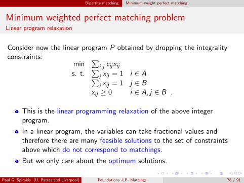
Consider now the linear program P obtained by dropping the integralityconstraints:
min∑
i ,j cijxijs. t.
∑j xij = 1 i ∈ A∑i xij = 1 j ∈ B
xij ≥ 0 i ∈ A, j ∈ B .
This is the linear programming relaxation of the above integerprogram.
In a linear program, the variables can take fractional values andtherefore there are many feasible solutions to the set of constraintsabove which do not correspond to matchings.
But we only care about the optimum solutions.
Paul G. Spirakis (U. Patras and Liverpool) Foundations -LP- Matcings 78 / 91
Bipartite matching Minimum weight perfect matching
Minimum weighted perfect matching problemLinear program relaxation
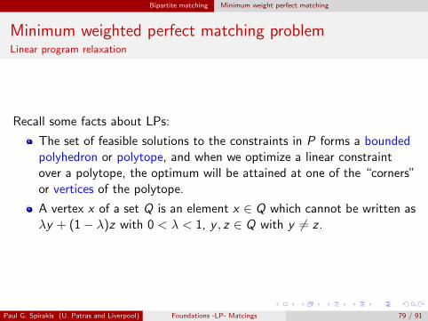
Recall some facts about LPs:
The set of feasible solutions to the constraints in P forms a boundedpolyhedron or polytope, and when we optimize a linear constraintover a polytope, the optimum will be attained at one of the “corners”or vertices of the polytope.
A vertex x of a set Q is an element x ∈ Q which cannot be written asλy + (1− λ)z with 0 < λ < 1, y , z ∈ Q with y 6= z .
Paul G. Spirakis (U. Patras and Liverpool) Foundations -LP- Matcings 79 / 91
Bipartite matching Minimum weight perfect matching
Minimum weighted perfect matching problemLinear program relaxation
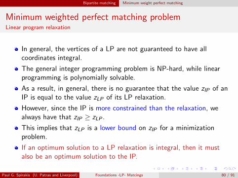
In general, the vertices of a LP are not guaranteed to have allcoordinates integral.
The general integer programming problem is NP-hard, while linearprogramming is polynomially solvable.
As a result, in general, there is no guarantee that the value zIP of anIP is equal to the value zLP of its LP relaxation.
However, since the IP is more constrained than the relaxation, wealways have that zIP ≥ zLP .
This implies that zLP is a lower bound on zIP for a minimizationproblem.
If an optimum solution to a LP relaxation is integral, then it mustalso be an optimum solution to the IP.
Paul G. Spirakis (U. Patras and Liverpool) Foundations -LP- Matcings 80 / 91
Bipartite matching Minimum weight perfect matching
Minimum weighted perfect matching problemPrimal-dual algorithm
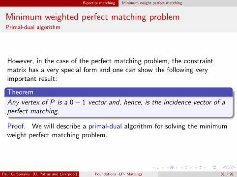
However, in the case of the perfect matching problem, the constraintmatrix has a very special form and one can show the following veryimportant result:
Theorem
Any vertex of P is a 0− 1 vector and, hence, is the incidence vector of aperfect matching.
Proof. We will describe a primal-dual algorithm for solving the minimumweight perfect matching problem.
Paul G. Spirakis (U. Patras and Liverpool) Foundations -LP- Matcings 81 / 91
Bipartite matching Minimum weight perfect matching
Minimum weighted perfect matching problemPrimal-dual algorithm
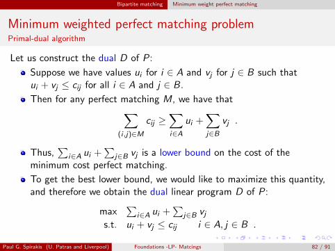
Let us construct the dual D of P:
Suppose we have values ui for i ∈ A and vj for j ∈ B such thatui + vj ≤ cij for all i ∈ A and j ∈ B.
Then for any perfect matching M, we have that∑(i ,j)∈M
cij ≥∑i∈A
ui +∑j∈B
vj .
Thus,∑
i∈A ui +∑
j∈B vj is a lower bound on the cost of theminimum cost perfect matching.
To get the best lower bound, we would like to maximize this quantity,and therefore we obtain the dual linear program D of P:
max∑
i∈A ui +∑
j∈B vjs.t. ui + vj ≤ cij i ∈ A, j ∈ B .
Paul G. Spirakis (U. Patras and Liverpool) Foundations -LP- Matcings 82 / 91
Bipartite matching Minimum weight perfect matching
Minimum weighted perfect matching problemPrimal-dual algorithm
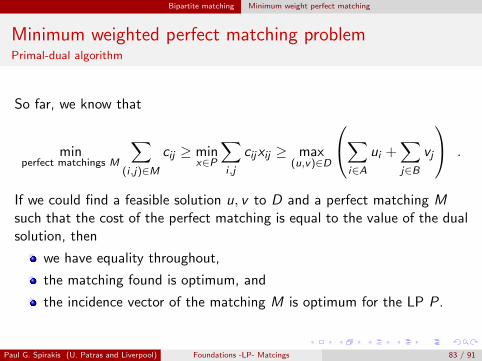
So far, we know that
minperfect matchings M
∑(i ,j)∈M
cij ≥ minx∈P
∑i ,j
cijxij ≥ max(u,v)∈D
∑i∈A
ui +∑j∈B
vj
.
If we could find a feasible solution u, v to D and a perfect matching Msuch that the cost of the perfect matching is equal to the value of the dualsolution, then
we have equality throughout,
the matching found is optimum, and
the incidence vector of the matching M is optimum for the LP P.
Paul G. Spirakis (U. Patras and Liverpool) Foundations -LP- Matcings 83 / 91
Bipartite matching Minimum weight perfect matching
Minimum weighted perfect matching problemPrimal-dual algorithm
Given a solution u, v to the dual, a perfect matching M would satisfyequality if it contains only edges (i , j) such that wij = cij − ui − vj = 0.⇒ This is what is referred to as complementary slackness.
The algorithm performs a series of iterations to obtain an appropriateu and v .
It always maintains a dual feasible solution and tries to find an“almost” primal feasible solution x satisfying complementaryslackness.
The fact that complementary slackness is imposed is crucial in anyprimal-dual algorithm.
Paul G. Spirakis (U. Patras and Liverpool) Foundations -LP- Matcings 84 / 91
Bipartite matching Minimum weight perfect matching
Minimum weighted perfect matching problemPrimal-dual algorithm
The algorithm works as follows.
It first starts with any dual feasible solution, say ui = 0 for all i andvj = mini cij for all j .
In a given iteration, the algorithm has a dual feasible solution (u, v)or say (u, v ,w).
Imposing complementary slackness means that we are interested inmatchings which are subgraphs of E = {(i , j) : wij = 0}.
Paul G. Spirakis (U. Patras and Liverpool) Foundations -LP- Matcings 85 / 91
Bipartite matching Minimum weight perfect matching
Minimum weighted perfect matching problemPrimal-dual algorithm
If E has a perfect matching then the incidence vector of thatmatching is a feasible solution in P and satisfies complementaryslackness with the current dual solution and, hence, must be optimal.
To check whether E has a perfect matching, one can use thecardinality matching algorithm we saw earlier.
If the maximum matching output is not perfect then the algorithmwill use information from the optimum vertex cover C ∗ to update thedual solution in such a way that the value of the dual solutionincreases (we are maximizing in the dual).
Paul G. Spirakis (U. Patras and Liverpool) Foundations -LP- Matcings 86 / 91
Bipartite matching Minimum weight perfect matching
Minimum weighted perfect matching problemPrimal-dual algorithm
As in the cardinality matching algorithm, consider the set L of verticeswhich can be reached by a directed path from an exposed vertex in A.
Then there is no edge of E between A ∩ L and B − L.
In other words, for every i ∈ (A ∩ L) and every j ∈ (B − L), we havewij = cij − ui − vj > 0.
Let δ = mini∈(A∩L), j∈(B−L) wij > 0.
The dual solution is updated as follows:
ui =
{ui i ∈ A− Lui + δ i ∈ A ∩ L
and vj =
{vj j ∈ B − Lvj − δ i ∈ B ∩ L
Paul G. Spirakis (U. Patras and Liverpool) Foundations -LP- Matcings 87 / 91
Bipartite matching Minimum weight perfect matching
Minimum weighted perfect matching problemPrimal-dual algorithm
The above dual solution is feasible, in the sense that thecorresponding vector w satisfies wij ≥ 0 for all i and j .
What is the value of the new dual solution?
The difference between the values of the new dual solution and theold dual solution is equal to:
δ(|A∩L|−|B∩L|) = δ(|A∩L|+|A−L|−|A−L|−|B∩L|) = δ(n/2−|C ∗|) .
where A has size n/2 and C ∗ is the optimum vertex cover for thebipartite graph with edge set E .
But by assumption |C ∗| < n/2, implying that the value of the dualsolution strictly increases.
Paul G. Spirakis (U. Patras and Liverpool) Foundations -LP- Matcings 88 / 91
Bipartite matching Minimum weight perfect matching
Minimum weighted perfect matching problemPrimal-dual algorithm
One repeats this procedure until the algorithm terminates.
At that point, we have an incidence vector of a perfect matching andalso a dual feasible solution which satisfy complementary slackness.
They must therefore be optimal and this proves the existence of anintegral optimum solution to P.
By carefully choosing the cost function, one can make any vertex bethe unique optimum solution to the linear program, and this showsthat any vertex is integral and hence is the incidence vector of aperfect matching.
Paul G. Spirakis (U. Patras and Liverpool) Foundations -LP- Matcings 89 / 91
Bipartite matching Minimum weight perfect matching
Minimum weighted perfect matching problemPrimal-dual algorithm
Proof that the algorithm terminates:
At least one more vertex of B must be reachable from an exposed vertexof A (and no vertex of B becomes unreachable), since an edge e = (i , j)with i ∈ (A ∩ L) and j ∈ B − L now has wij = 0 by our choice of δ.
This also gives an estimate of the number of iterations:
In at most n/2 iterations, all vertices of B are reachable or thematching found has increased by at least one unit.
Therefore, after O(n2) iterations, the matching found is perfect.
The overall running time of the algorithm is thus O(n4) since it takesO(n2) to compute the set L in each iteration.
By looking more closely at how vertices get labeled, one can reducethe running time analysis to O(n3).
Paul G. Spirakis (U. Patras and Liverpool) Foundations -LP- Matcings 90 / 91
Further reading
J. H. van Lint and R. M. Wilson: A Course in Combinatorics.Cambridge University Press, 2006.
Reinhard Diestel: Graph Theory. 4th electronic edition, 2010.
Vasek Chvatal: Linear Programming. W. H. Freeman, 1983.
Paul G. Spirakis (U. Patras and Liverpool) Foundations -LP- Matcings 91 / 91


