Manifolds and Differential Forms
Reyer Sjamaar
Department of Mathematics, Cornell University, Ithaca, New York 14853-4201
E-mail address: [email protected]: http://www.math.cornell.edu/~sjamaar
Revised edition, 2017Copyright © Reyer Sjamaar, 2001, 2015, 2017. Paper or electronic copies for
personal use may be made without explicit permission from the author. All otherrights reserved.
Contents
Preface v
Chapter 1. Introduction 11.1. Manifolds 11.2. Equations 71.3. Parametrizations 91.4. Configuration spaces 10Exercises 14
Chapter 2. Differential forms on Euclidean space 172.1. Elementary properties 172.2. The exterior derivative 202.3. Closed and exact forms 222.4. The Hodge star operator 242.5. div, grad and curl 25Exercises 27
Chapter 3. Pulling back forms 313.1. Determinants 313.2. Pulling back forms 38Exercises 45
Chapter 4. Integration of 1-forms 494.1. Definition and elementary properties of the integral 494.2. Integration of exact 1-forms 514.3. Angle functions and the winding number 54Exercises 58
Chapter 5. Integration and Stokes’ theorem 635.1. Integration of forms over chains 635.2. The boundary of a chain 665.3. Cycles and boundaries 685.4. Stokes’ theorem 70Exercises 71
Chapter 6. Manifolds 756.1. The definition 756.2. The regular value theorem 82Exercises 88
Chapter 7. Differential forms on manifolds 91
iii
iv CONTENTS
7.1. First definition 917.2. Second definition 92Exercises 99
Chapter 8. Volume forms 1018.1. n-Dimensional volume in RN 1018.2. Orientations 1048.3. Volume forms 107Exercises 111
Chapter 9. Integration and Stokes’ theorem for manifolds 1139.1. Manifolds with boundary 1139.2. Integration over orientable manifolds 1179.3. Gauss and Stokes 120Exercises 122
Chapter 10. Applications to topology 12510.1. Brouwer’s fixed point theorem 12510.2. Homotopy 12610.3. Closed and exact forms re-examined 131Exercises 136
Appendix A. Sets and functions 139A.1. Glossary 139A.2. General topology of Euclidean space 141Exercises 142
Appendix B. Calculus review 145B.1. The fundamental theorem of calculus 145B.2. Derivatives 145B.3. The chain rule 148B.4. The implicit function theorem 149B.5. The substitution formula for integrals 151Exercises 151
Appendix C. The Greek alphabet 155
Bibliography 157
Notation Index 159
Index 161
Preface
These are the lecture notes for Math 3210 (formerly named Math 321), Mani-folds and Differential Forms, as taught at Cornell University since the Fall of 2001.The course covers manifolds and differential forms for an audience of undergrad-uates who have taken a typical calculus sequence at a North American university,including basic linear algebra and multivariable calculus up to the integral theo-rems of Green, Gauss and Stokes. With a view to the fact that vector spaces arenowadays a standard item on the undergraduate menu, the text is not restricted tocurves and surfaces in three-dimensional space, but treats manifolds of arbitrarydimension. Some prerequisites are briefly reviewed within the text and in appen-dices. The selection of material is similar to that in Spivak’s book [Spi71] and inFlanders’ book [Fla89], but the treatment is at a more elementary and informallevel appropriate for sophomores and juniors.
A large portion of the text consists of problem sets placed at the end of eachchapter. The exercises range from easy substitution drills to fairly involved but, Ihope, interesting computations, as well as more theoretical or conceptual problems.More than once the text makes use of results obtained in the exercises.
Because of its transitional nature between calculus and analysis, a text of thiskind has to walk a thin line between mathematical informality and rigour. I havetended to err on the side of caution by providing fairly detailed definitions andproofs. In class, depending on the aptitudes and preferences of the audience andalso on the available time, one can skip over many of the details without too muchloss of continuity. At any rate, most of the exercises do not require a great deal offormal logical skill and throughout I have tried to minimize the use of point-settopology.
These notes, occasionally revised and updated, are available athttp://www.math.cornell.edu/~sjamaar/manifolds/.
Corrections, suggestions and comments sent to [email protected] bereceived gratefully.
Ithaca, New York, December 2017
v

CHAPTER 1
Introduction
We start with an informal, intuitive introduction to manifolds and how theyarise in mathematical nature. Most of this material will be examined more thor-oughly in later chapters.
1.1. Manifolds
Recall that Euclidean n-space Rn is the set of all column vectors with n realentries
x
*....,
x1
x2
...xn
+////-,
which we shall call points or n-vectors and denote by lower case boldface letters. InR2 or R3 we often write
x
(
xy
)
, resp. x
*.,
xyz
+/-.
For reasons having to do with matrix multiplication, column vectors are not to beconfused with row vectors (x1 x2 · · · xn ). Nevertheless, to save space we shallfrequently write a column vector x as an n-tuple
x (x1 , x2 , . . . , xn )
with the entries separated by commas.A manifold is a certain type of subset of Rn . A precise definition will follow
in Chapter 6, but one important consequence of the definition is that at each of itspoints a manifold has a well-defined tangent space, which is a linear subspace ofRn . This fact enables us to apply the methods of calculus and linear algebra to thestudy of manifolds. The dimension of a manifold is by definition the dimension ofany of its tangent spaces. The dimension of a manifold in Rn can be no higher thann.
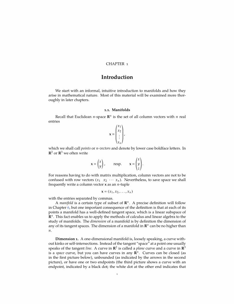
Dimension 1. A one-dimensional manifold is, loosely speaking, a curve with-out kinks or self-intersections. Instead of the tangent “space” at a point one usuallyspeaks of the tangent line. A curve in R2 is called a plane curve and a curve in R3
is a space curve, but you can have curves in any Rn . Curves can be closed (asin the first picture below), unbounded (as indicated by the arrows in the secondpicture), or have one or two endpoints (the third picture shows a curve with anendpoint, indicated by a black dot; the white dot at the other end indicates that
1
2 1. INTRODUCTION
that point does not belong to the curve; the curve “peters out” without coming toan endpoint). Endpoints are also called boundary points.
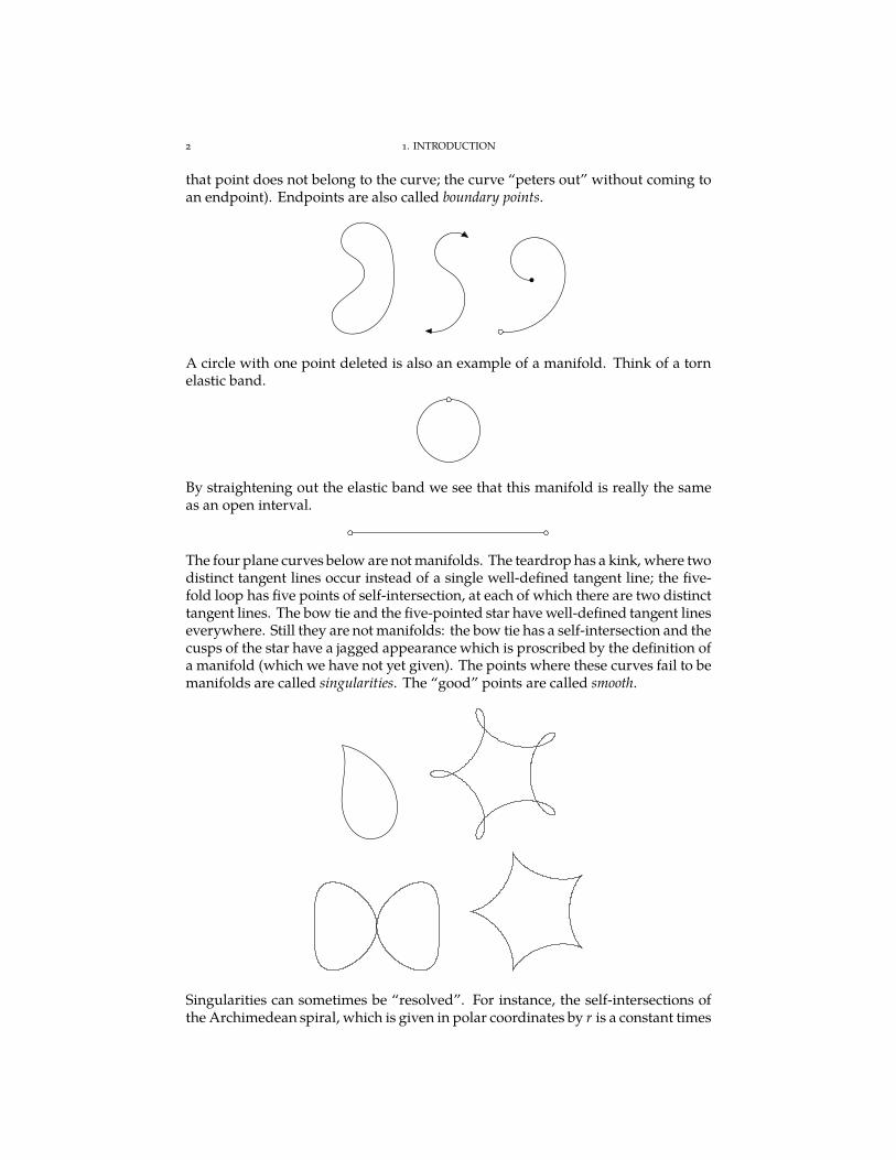
A circle with one point deleted is also an example of a manifold. Think of a tornelastic band.
By straightening out the elastic band we see that this manifold is really the sameas an open interval.
The four plane curves below are not manifolds. The teardrop has a kink, where twodistinct tangent lines occur instead of a single well-defined tangent line; the five-fold loop has five points of self-intersection, at each of which there are two distincttangent lines. The bow tie and the five-pointed star have well-defined tangent lineseverywhere. Still they are not manifolds: the bow tie has a self-intersection and thecusps of the star have a jagged appearance which is proscribed by the definition ofa manifold (which we have not yet given). The points where these curves fail to bemanifolds are called singularities. The “good” points are called smooth.
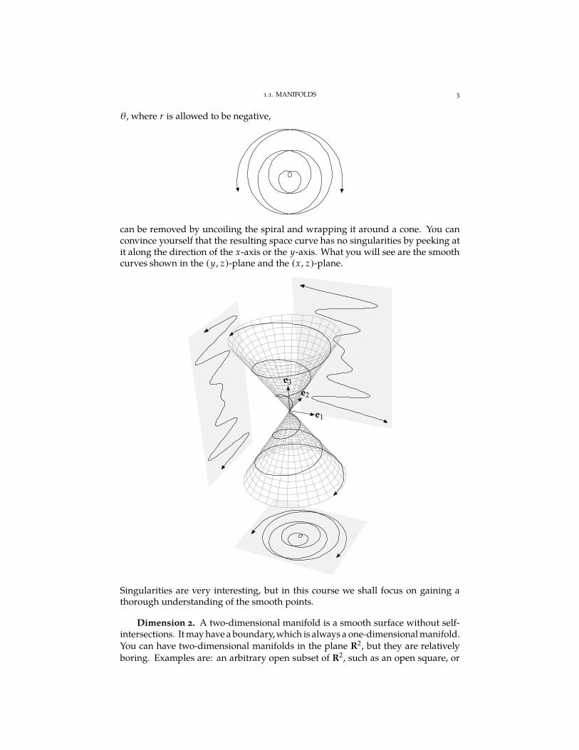
Singularities can sometimes be “resolved”. For instance, the self-intersections ofthe Archimedean spiral, which is given in polar coordinates by r is a constant times
1.1. MANIFOLDS 3
θ, where r is allowed to be negative,
can be removed by uncoiling the spiral and wrapping it around a cone. You canconvince yourself that the resulting space curve has no singularities by peeking atit along the direction of the x-axis or the y-axis. What you will see are the smoothcurves shown in the (y , z)-plane and the (x , z)-plane.
e1
e2
e3
Singularities are very interesting, but in this course we shall focus on gaining athorough understanding of the smooth points.
Dimension 2. A two-dimensional manifold is a smooth surface without self-intersections. It may have a boundary,which is always a one-dimensional manifold.You can have two-dimensional manifolds in the plane R2, but they are relativelyboring. Examples are: an arbitrary open subset of R2, such as an open square, or
4 1. INTRODUCTION
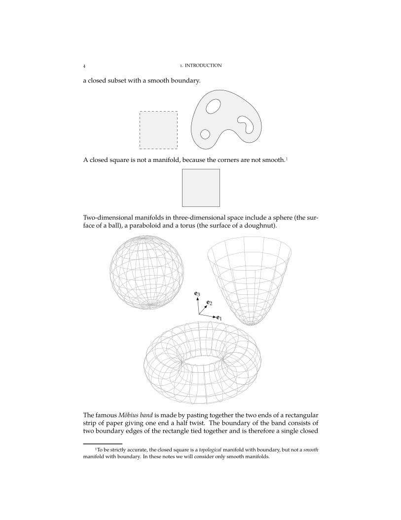
a closed subset with a smooth boundary.
A closed square is not a manifold, because the corners are not smooth.1
Two-dimensional manifolds in three-dimensional space include a sphere (the sur-face of a ball), a paraboloid and a torus (the surface of a doughnut).
e1
e2
e3
The famous Möbius band is made by pasting together the two ends of a rectangularstrip of paper giving one end a half twist. The boundary of the band consists oftwo boundary edges of the rectangle tied together and is therefore a single closed
1To be strictly accurate, the closed square is a topological manifold with boundary, but not a smooth
manifold with boundary. In these notes we will consider only smooth manifolds.
1.1. MANIFOLDS 5
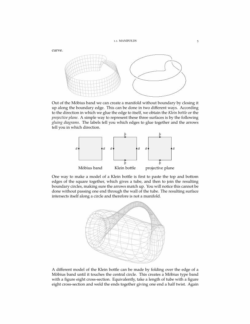
curve.
Out of the Möbius band we can create a manifold without boundary by closing itup along the boundary edge. This can be done in two different ways. Accordingto the direction in which we glue the edge to itself, we obtain the Klein bottle or theprojective plane. A simple way to represent these three surfaces is by the followinggluing diagrams. The labels tell you which edges to glue together and the arrowstell you in which direction.
a a
Möbius band
a a
b
b
Klein bottle
a a
b
b
projective plane
One way to make a model of a Klein bottle is first to paste the top and bottomedges of the square together, which gives a tube, and then to join the resultingboundary circles, making sure the arrows match up. You will notice this cannot bedone without passing one end through the wall of the tube. The resulting surfaceintersects itself along a circle and therefore is not a manifold.
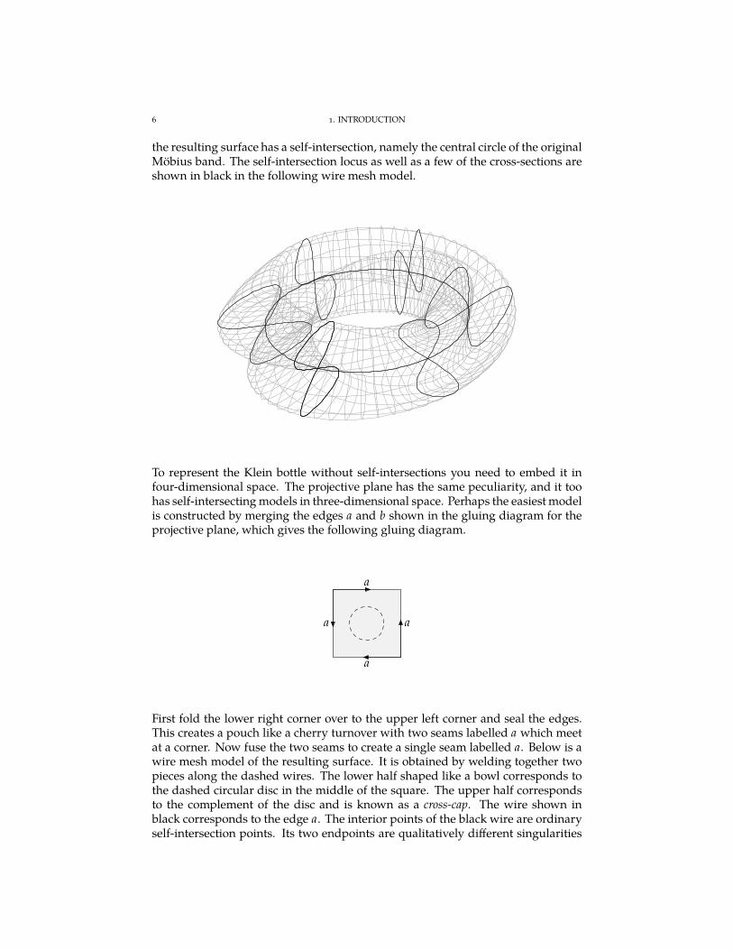
A different model of the Klein bottle can be made by folding over the edge of aMöbius band until it touches the central circle. This creates a Möbius type bandwith a figure eight cross-section. Equivalently, take a length of tube with a figureeight cross-section and weld the ends together giving one end a half twist. Again
6 1. INTRODUCTION
the resulting surface has a self-intersection, namely the central circle of the originalMöbius band. The self-intersection locus as well as a few of the cross-sections areshown in black in the following wire mesh model.
To represent the Klein bottle without self-intersections you need to embed it infour-dimensional space. The projective plane has the same peculiarity, and it toohas self-intersecting models in three-dimensional space. Perhaps the easiest modelis constructed by merging the edges a and b shown in the gluing diagram for theprojective plane, which gives the following gluing diagram.
a a
a
a
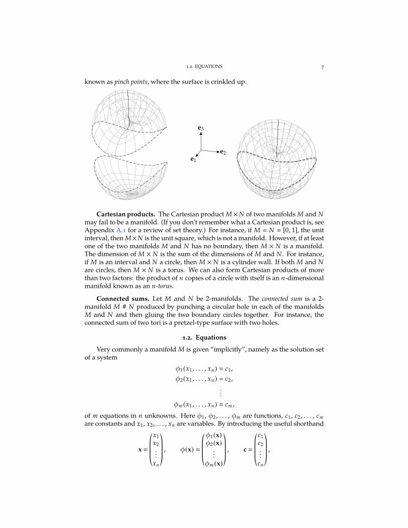
First fold the lower right corner over to the upper left corner and seal the edges.This creates a pouch like a cherry turnover with two seams labelled a which meetat a corner. Now fuse the two seams to create a single seam labelled a. Below is awire mesh model of the resulting surface. It is obtained by welding together twopieces along the dashed wires. The lower half shaped like a bowl corresponds tothe dashed circular disc in the middle of the square. The upper half correspondsto the complement of the disc and is known as a cross-cap. The wire shown inblack corresponds to the edge a. The interior points of the black wire are ordinaryself-intersection points. Its two endpoints are qualitatively different singularities
1.2. EQUATIONS 7
known as pinch points, where the surface is crinkled up.
e1
e2
e3
Cartesian products. The Cartesian product M ×N of two manifolds M and Nmay fail to be a manifold. (If you don’t remember what a Cartesian product is, seeAppendix A.1 for a review of set theory.) For instance, if M N [0, 1], the unitinterval, then M×N is the unit square, which is not a manifold. However, if at leastone of the two manifolds M and N has no boundary, then M × N is a manifold.The dimension of M × N is the sum of the dimensions of M and N . For instance,if M is an interval and N a circle, then M × N is a cylinder wall. If both M and Nare circles, then M × N is a torus. We can also form Cartesian products of morethan two factors: the product of n copies of a circle with itself is an n-dimensionalmanifold known as an n-torus.
Connected sums. Let M and N be 2-manifolds. The connected sum is a 2-manifold M # N produced by punching a circular hole in each of the manifoldsM and N and then gluing the two boundary circles together. For instance, theconnected sum of two tori is a pretzel-type surface with two holes.
1.2. Equations
Very commonly a manifold M is given “implicitly”, namely as the solution setof a system
φ1(x1 , . . . , xn) c1 ,
φ2(x1 , . . . , xn) c2 ,
...
φm (x1 , . . . , xn) cm ,
of m equations in n unknowns. Here φ1, φ2 , . . . , φm are functions, c1, c2 , . . . , cm
are constants and x1, x2 , . . . , xn are variables. By introducing the useful shorthand
x
*....,
x1
x2
...xn
+////-, φ(x)
*....,
φ1(x)
φ2(x)...
φm (x)
+////-, c
*....,
c1
c2
...cn
+////-,
8 1. INTRODUCTION
we can represent this system as a single equation
φ(x) c.
The solution set M is the set of all vectors x in Rn which satisfy φ(x) c and isdenoted by φ−1(c). (This notation is standard, but a bit unfortunate because itsuggests falsely that φ is invertible, which it is usually not.) Thus
M φ−1(c) x ∈ Rn | φ(x) c .It is in general difficult to find explicit solutions of a system of equations. (On thepositive side, it is usually easy to decide whether any given point is a solution byplugging it into the equations.) Manifolds defined by linear equations (i.e. whereφ is a matrix) are called affine subspaces of Rn and are studied in linear algebra.More interesting manifolds arise from nonlinear equations.
1.1. Example. The simplest case is that of a single equation (m 1), such as
x2 + y2 − z2 0.
Here we have a single scalar-valued function of three variables φ(x , y , z) x2 +
y2 − z2 and c 0. The solution set M of the equation is a cone in R3, which isnot a manifold because it has no well-defined tangent plane at the origin. We candetermine the tangent plane at any other point of M by recalling from calculusthat the gradient of φ is perpendicular to the surface. Hence for any nonzero x
(x , y , z) ∈ M the tangent plane to M at x is the plane perpendicular to grad(φ)(x)
(2x , 2y ,−2z).
As we see from this example, the solution set of a system of equations mayhave singularities and is therefore not necessarily a manifold. In general, if M isgiven by a single equation φ(x) c and x is a point of M with the property thatgrad(φ)(x) , 0, then x is a smooth point of M and the tangent space at x is theorthogonal complement of grad(φ)(x). (Conversely, if x is a singular point of M,we must have grad(φ)(x) 0!) The standard notation for the tangent space to Mat x is TxM. Thus we can write TxM grad(φ)(x)⊥.
1.2. Example. The sphere of radius r about the origin in Rn is the set of all x inRn satisfying the single equation ‖x‖ r. Here
‖x‖ √
x · x
√
x21
+ x22
+ · · · + x2n
is the norm or length of x and
x · y xTy x1 y1 + x2 y2 + · · · + xn yn
is the inner product or dot product of x and y. The sphere of radius r is an n − 1-dimensional manifold in Rn . The sphere of radius 1 is called the unit sphere andis denoted by Sn−1. In particular, the one-dimensional unit “sphere” S1 is the unitcircle in the plane, and the zero-dimensional unit “sphere” S0 is the subset −1, 1of the real line. To determine the tangent spaces of the unit sphere it is easierto work with the equation ‖x‖2 1 instead of ‖x‖ 1. In other words, we letφ(x) ‖x‖2. Then grad(φ)(x) 2x, which is nonzero for all x in the unit sphere.Therefore Sn−1 is a manifold and for any x in Sn−1 we have
TxSn−1 (2x)⊥ x⊥ y ∈ Rn | y · x 0 ,
1.3. PARAMETRIZATIONS 9
a linear subspace of Rn . (In Exercise 1.7 you will be asked to find a basis of thetangent space for a particular x and you will see that TxSn−1 is n − 1-dimensional.)
1.3. Example. Consider the system of two equations in three unknowns,
x2 + y2 1,
y + z 0.
Here
φ(x)
(
x2 + y2
y + z
)
and c
(
10
)
.
The solution set of this system is the intersection of a cylinder of radius 1 aboutthe z-axis (given by the first equation) and a plane cutting the x-axis at a 45 angle(given by the second equation). Hence the solution set is an ellipse. It is a manifoldof dimension 1. We will discuss in Chapter 6 how to find the tangent spaces tomanifolds given by more than one equation.
Inequalities. Manifolds with boundary are often presented as solution setsof a system of equations together with one or more inequalities. For instance, theclosed ball of radius r about the origin in Rn is given by the single inequality ‖x‖ ≤ r.Its boundary is the sphere of radius r.
1.3. Parametrizations
A dual method for describing manifolds is the “explicit” way, namely by par-ametrizations. For instance,
x cos θ, y sin θ
parametrizes the unit circle in R2 and
x cos θ cosφ, y sin θ cosφ, z sin φ
parametrizes the unit sphere in R3. (Here φ is the angle between a vector andthe (x , y)-plane and θ is the polar angle in the (x , y)-plane.) The explicit methodhas various merits and demerits, which are complementary to those of the im-plicit method. One obvious advantage is that it is easy to find points lying on aparametrized manifold simply by plugging in values for the parameters. A disad-vantage is that it can be hard to decide if any given point is on the manifold or not,because this involves solving for the parameters. Parametrizations are often harderto come by than a system of equations, but are at times more useful, for examplewhen one wants to integrate over the manifold. Also, it is usually impossible toparametrize a manifold in such a way that every point is covered exactly once.Such is the case for the two-sphere. One commonly restricts the polar coordinates(θ, φ) to the rectangle [0, 2π] × [−π/2, π/2] to avoid counting points twice. Onlythe meridian θ 0 is then hit twice, but this does not matter for many purposes,such as computing the surface area or integrating a continuous function.
We will use parametrizations to give a formal definition of the notion of amanifold in Chapter 6. Note however that not every parametrization describes amanifold.
10 1. INTRODUCTION
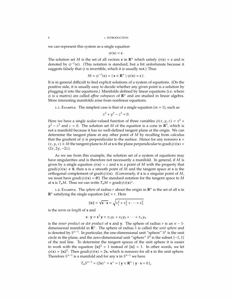
1.4. Example. Define c(t) (t2 , t3) for t ∈ R. As t runs through the real line,the point c(t) travels along a curve in the plane, which we call a path or parametrizedcurve.
The path c has no self-intersections: if t1 , t2 then c(t1) , c(t2). The cusp at theorigin (t 0) is a singular point, but all other points (t , 0) are smooth. The tangentline at a smooth point c(t) is the line spanned by the velocity vector c′(t) (2t , 3t2).The slope of the tangent line is 3t2/2t 3
2 t. For t 0 the velocity vector is c′(0) 0,which does not span a line. Nevertheless, the curve has a well-defined (horizontal)tangent line at the origin, which we can think of as the limit of the tangent lines ast tends to 0.
More examples of parametrizations are given in Exercises 1.1–1.3.
1.4. Configuration spaces
Frequently manifolds arise in more abstract ways that may be hard to capturein terms of equations or parametrizations. Examples are solution curves of differ-ential equations (see e.g. Exercise 1.11) and configuration spaces. The configurationor state of a mechanical system (such as a pendulum, a spinning top, the solarsystem, a fluid, or a gas etc.) is a complete specification of the position of each of itsparts. (The configuration ignores any motions that the system may be undergoing.So a configuration is like a snapshot or a movie still. When the system moves, itsconfiguration changes.) The configuration space or state space of the system is an ab-stract space, the points of which are in one-to-one correspondence to all physicallypossible configurations of the system. Very often the configuration space turnsout to be a manifold. Its dimension is called the number of degrees of freedom of thesystem.
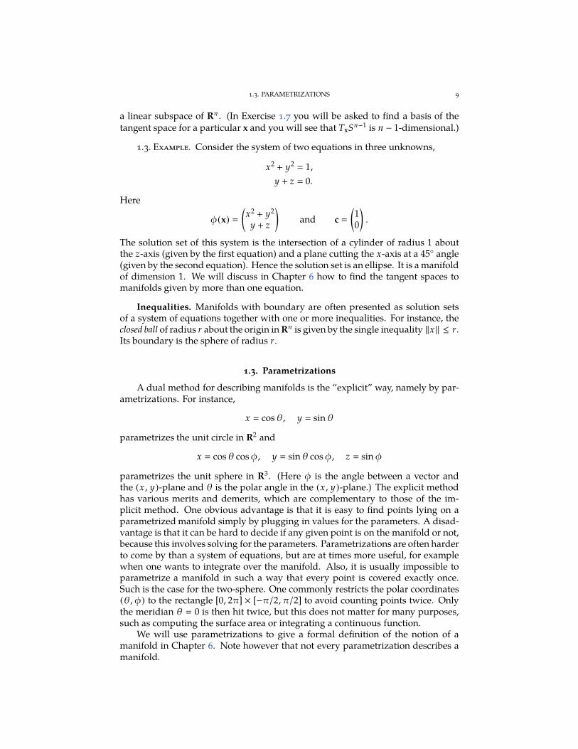
1.5. Example. A spherical pendulum is a weight or bob attached to a fixed centreby a rigid rod, free to swing in any direction in three-space.
The state of the pendulum is entirely determined by the position of the bob. Thebob can move from any point at a fixed distance (equal to the length of the rod) fromthe centre to any other. The configuration space is therefore a two-dimensionalsphere, and the spherical pendulum has two degrees of freedom.
The configuration space of even a fairly small system can be quite complicated.Even if the system is situated in three-dimensional space, it may have many more
1.4. CONFIGURATION SPACES 11
than three degrees of freedom. This is why higher-dimensional manifolds arecommon in physics and applied mathematics.
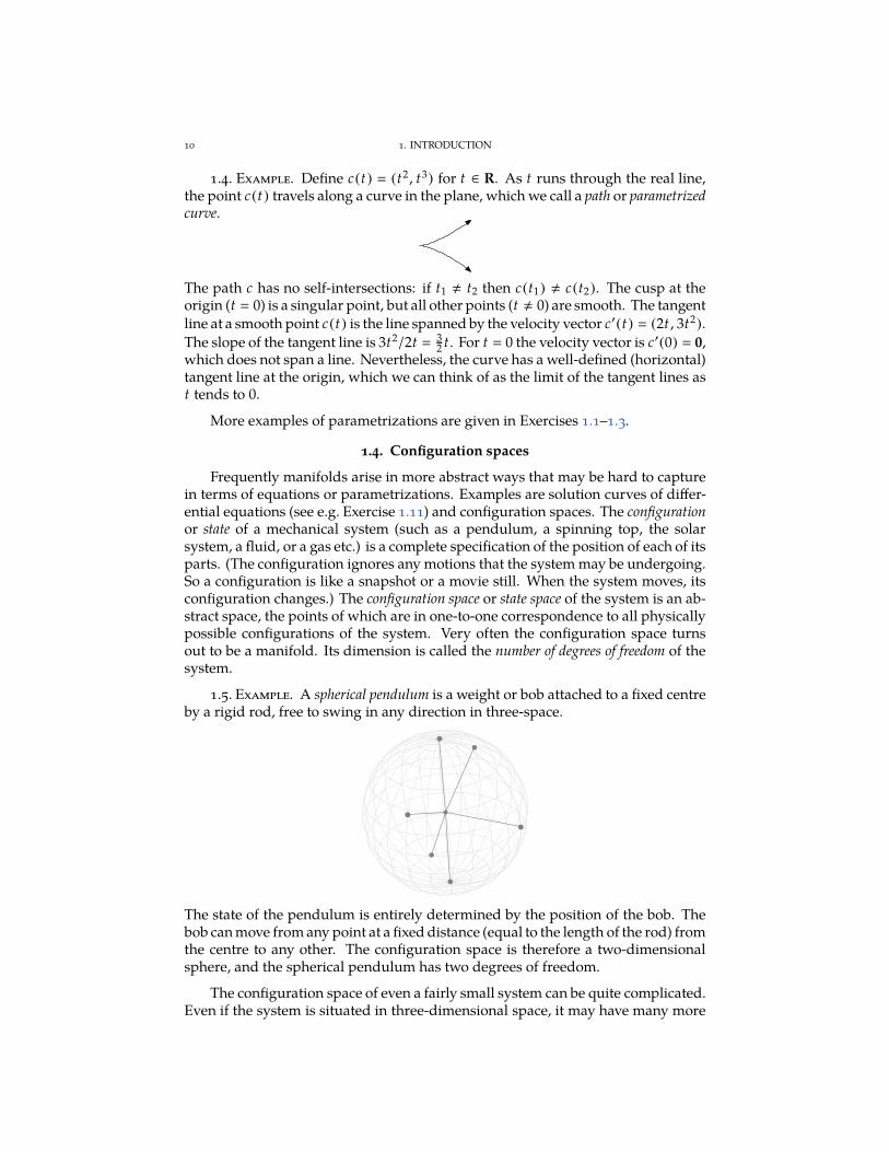
1.6. Example. Take a spherical pendulum of length r and attach a second oneof length s to the moving end of the first by a universal joint. The resulting systemis a double spherical pendulum. The state of this system can be specified by a pair ofvectors (x, y), x being the vector pointing from the centre to the first weight and ythe vector pointing from the first to the second weight.
x
y
The vector x is constrained to a sphere of radius r about the centre and y to a sphereof radius s about the head of x. Aside from this limitation, every pair of vectorscan occur (if we suppose the second rod is allowed to swing completely freely andmove “through” the first rod) and describes a distinct configuration. Thus there arefour degrees of freedom. The configuration space is a four-dimensional manifold,namely the Cartesian product of two two-dimensional spheres.
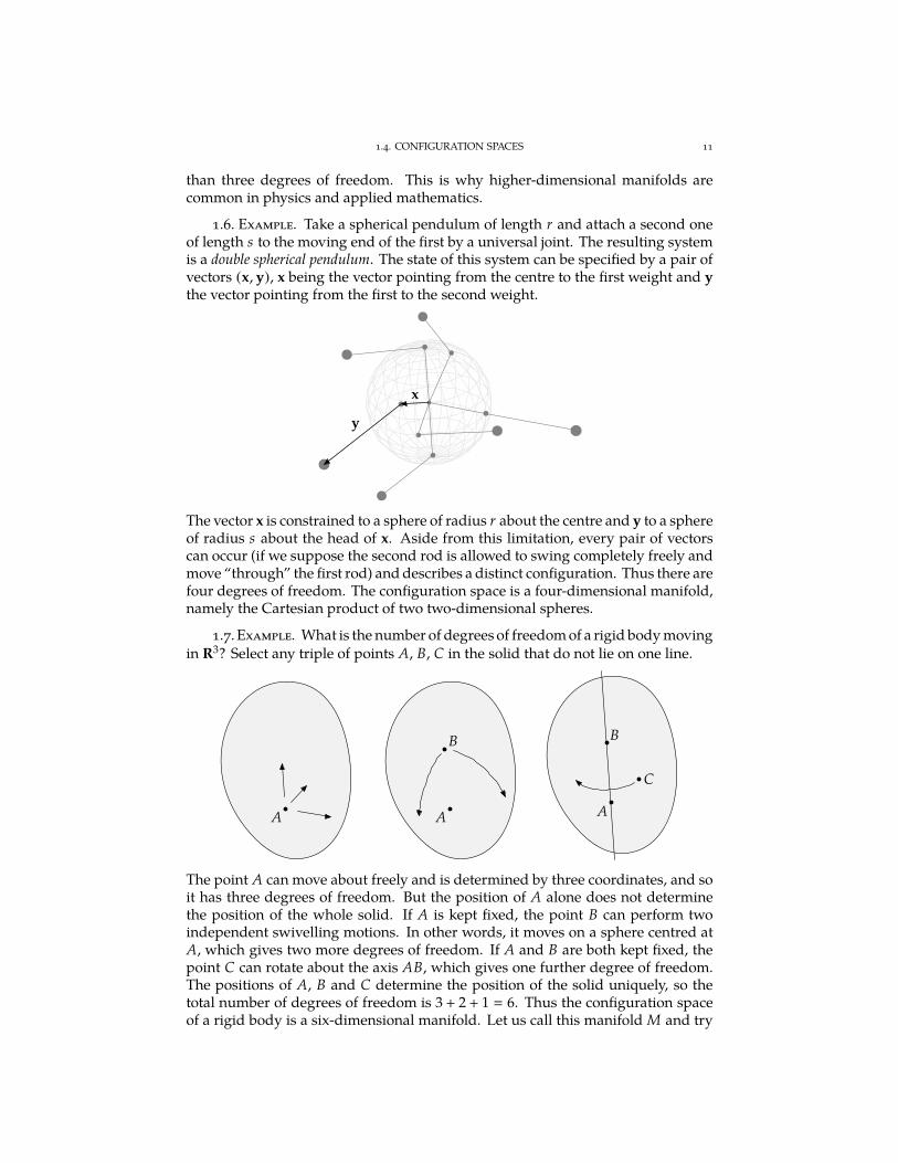
1.7. Example. What is the number of degrees of freedom of a rigid body movingin R3? Select any triple of points A, B, C in the solid that do not lie on one line.
A A
B
A
B
C
The point A can move about freely and is determined by three coordinates, and soit has three degrees of freedom. But the position of A alone does not determinethe position of the whole solid. If A is kept fixed, the point B can perform twoindependent swivelling motions. In other words, it moves on a sphere centred atA, which gives two more degrees of freedom. If A and B are both kept fixed, thepoint C can rotate about the axis AB, which gives one further degree of freedom.The positions of A, B and C determine the position of the solid uniquely, so thetotal number of degrees of freedom is 3 + 2 + 1 6. Thus the configuration spaceof a rigid body is a six-dimensional manifold. Let us call this manifold M and try
12 1. INTRODUCTION
to say something about its shape. Choose an arbitrary reference point in space.Inside the manifold M we have a subset M0 consisting of all configurations whichhave the point A placed at the reference point. Configurations in M0 have threefewer degrees of freedom, because only the points B and C can move, so M0 is athree-dimensional manifold. Every configuration in M can be moved to a uniqueconfiguration in M0 by a unique parallel translation of the solid which moves Ato the reference point. In other words, the points of M can be viewed as pairsconsisting of a point in M0 and a vector in R3: the manifold M is the Cartesianproduct M0 × R3. See Exercise 8.6 for more information on M0.
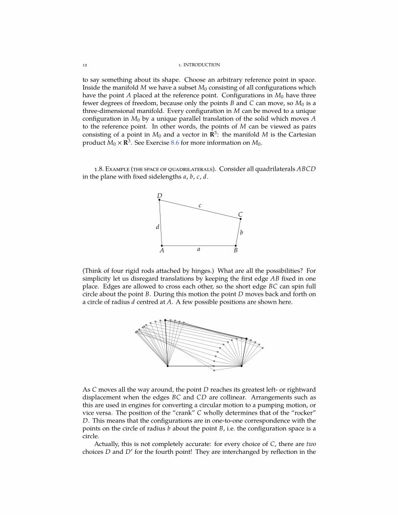
1.8. Example (the space of quadrilaterals). Consider all quadrilaterals ABCDin the plane with fixed sidelengths a, b, c, d.
A B
C
D
a
b
c
d
(Think of four rigid rods attached by hinges.) What are all the possibilities? Forsimplicity let us disregard translations by keeping the first edge AB fixed in oneplace. Edges are allowed to cross each other, so the short edge BC can spin fullcircle about the point B. During this motion the point D moves back and forth ona circle of radius d centred at A. A few possible positions are shown here.
As C moves all the way around, the point D reaches its greatest left- or rightwarddisplacement when the edges BC and CD are collinear. Arrangements such asthis are used in engines for converting a circular motion to a pumping motion, orvice versa. The position of the “crank” C wholly determines that of the “rocker”D. This means that the configurations are in one-to-one correspondence with thepoints on the circle of radius b about the point B, i.e. the configuration space is acircle.
Actually, this is not completely accurate: for every choice of C, there are twochoices D and D′ for the fourth point! They are interchanged by reflection in the
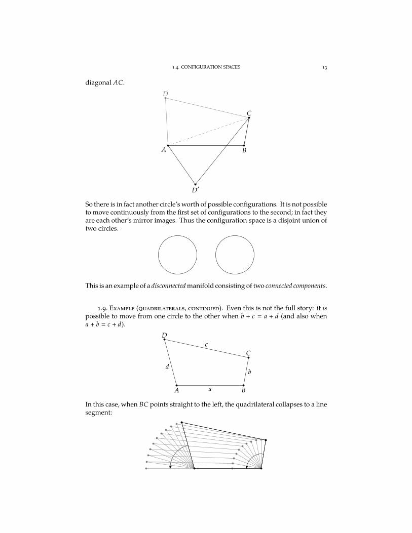
1.4. CONFIGURATION SPACES 13
diagonal AC.
A B
C
D
D′
So there is in fact another circle’s worth of possible configurations. It is not possibleto move continuously from the first set of configurations to the second; in fact theyare each other’s mirror images. Thus the configuration space is a disjoint union oftwo circles.
This is an example of a disconnected manifold consisting of two connected components.
1.9. Example (quadrilaterals, continued). Even this is not the full story: it ispossible to move from one circle to the other when b + c a + d (and also whena + b c + d).
A B
C
D
a
b
c
d
In this case, when BC points straight to the left, the quadrilateral collapses to a linesegment:
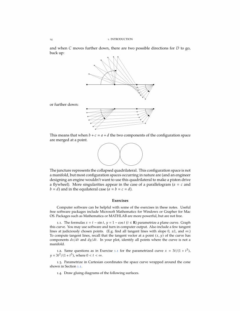
14 1. INTRODUCTION
and when C moves further down, there are two possible directions for D to go,back up:
or further down:
This means that when b + c a + d the two components of the configuration spaceare merged at a point.
The juncture represents the collapsed quadrilateral. This configuration space is nota manifold, but most configuration spaces occurring in nature are (and an engineerdesigning an engine wouldn’t want to use this quadrilateral to make a piston drivea flywheel). More singularities appear in the case of a parallelogram (a c andb d) and in the equilateral case (a b c d).
Exercises
Computer software can be helpful with some of the exercises in these notes. Usefulfree software packages include Microsoft Mathematics for Windows or Grapher for MacOS. Packages such as Mathematica or MATHLAB are more powerful, but are not free.
1.1. The formulas x t − sin t, y 1 − cos t (t ∈ R) parametrize a plane curve. Graphthis curve. You may use software and turn in computer output. Also include a few tangentlines at judiciously chosen points. (E.g. find all tangent lines with slope 0, ±1, and ∞.)To compute tangent lines, recall that the tangent vector at a point (x, y) of the curve hascomponents dx/dt and dy/dt. In your plot, identify all points where the curve is not amanifold.
1.2. Same questions as in Exercise 1.1 for the parametrized curve x 3t/(1 + t3),
y 3t2/(1 + t3), where 0 < t < ∞.
1.3. Parametrize in Cartesian coordinates the space curve wrapped around the coneshown in Section 1.1.
1.4. Draw gluing diagrams of the following surfaces.
EXERCISES 15
(i) A sphere.(ii) A torus with a hole punched in it.
(iii) The connected sum of two tori.
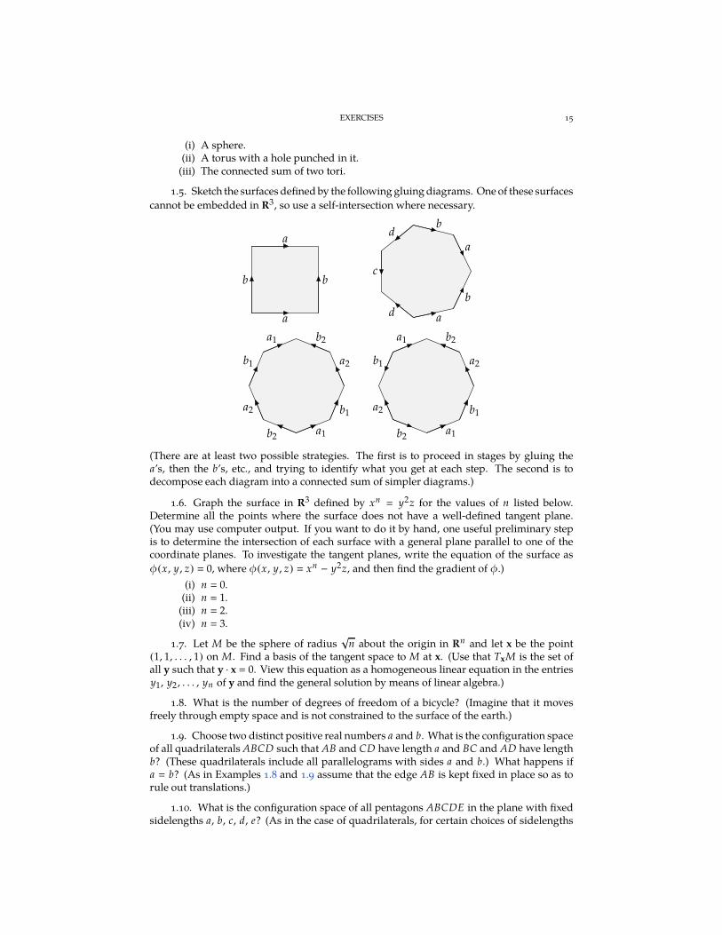
1.5. Sketch the surfaces defined by the following gluing diagrams. One of these surfaces
cannot be embedded in R3, so use a self-intersection where necessary.
a
a
b b
a
b
a
bd
c
d
a1
b1
a2
b2a1
b1
a2
b2a1
b1
a2
b2a1
b1
a2
b2
(There are at least two possible strategies. The first is to proceed in stages by gluing thea’s, then the b’s, etc., and trying to identify what you get at each step. The second is todecompose each diagram into a connected sum of simpler diagrams.)
1.6. Graph the surface in R3 defined by xn y2z for the values of n listed below.
Determine all the points where the surface does not have a well-defined tangent plane.(You may use computer output. If you want to do it by hand, one useful preliminary stepis to determine the intersection of each surface with a general plane parallel to one of thecoordinate planes. To investigate the tangent planes, write the equation of the surface as
φ(x, y , z) 0, where φ(x, y , z) xn − y2z, and then find the gradient of φ.)
(i) n 0.(ii) n 1.
(iii) n 2.(iv) n 3.
1.7. Let M be the sphere of radius√
n about the origin in Rn and let x be the point(1, 1, . . . , 1) on M. Find a basis of the tangent space to M at x. (Use that TxM is the set ofall y such that y · x 0. View this equation as a homogeneous linear equation in the entriesy1, y2 , . . . , yn of y and find the general solution by means of linear algebra.)
1.8. What is the number of degrees of freedom of a bicycle? (Imagine that it movesfreely through empty space and is not constrained to the surface of the earth.)
1.9. Choose two distinct positive real numbers a and b. What is the configuration spaceof all quadrilaterals ABCD such that AB and CD have length a and BC and AD have lengthb? (These quadrilaterals include all parallelograms with sides a and b.) What happens ifa b? (As in Examples 1.8 and 1.9 assume that the edge AB is kept fixed in place so as torule out translations.)
1.10. What is the configuration space of all pentagons ABCDE in the plane with fixedsidelengths a, b, c, d, e? (As in the case of quadrilaterals, for certain choices of sidelengths
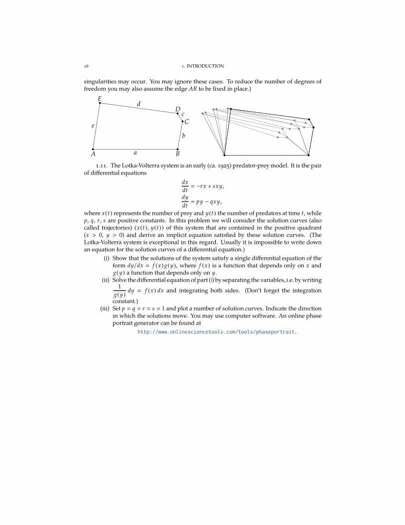
16 1. INTRODUCTION
singularities may occur. You may ignore these cases. To reduce the number of degrees offreedom you may also assume the edge AB to be fixed in place.)
A B
C
D
E
a
b
c
d
e
1.11. The Lotka-Volterra system is an early (ca. 1925) predator-prey model. It is the pairof differential equations
dx
dt −rx + sxy ,
dy
dt py − qxy ,
where x(t) represents the number of prey and y(t) the number of predators at time t, whilep, q, r, s are positive constants. In this problem we will consider the solution curves (alsocalled trajectories) (x(t), y(t)) of this system that are contained in the positive quadrant(x > 0, y > 0) and derive an implicit equation satisfied by these solution curves. (TheLotka-Volterra system is exceptional in this regard. Usually it is impossible to write downan equation for the solution curves of a differential equation.)
(i) Show that the solutions of the system satisfy a single differential equation of theform dy/dx f (x)g(y), where f (x) is a function that depends only on x andg(y) a function that depends only on y.
(ii) Solve the differential equation of part (i) by separating the variables, i.e. by writing1
g(y)dy f (x) dx and integrating both sides. (Don’t forget the integration
constant.)(iii) Set p q r s 1 and plot a number of solution curves. Indicate the direction
in which the solutions move. You may use computer software. An online phaseportrait generator can be found at
http://www.onlinesciencetools.com/tools/phaseportrait .
CHAPTER 2
Differential forms on Euclidean space
The notion of a differential form encompasses such ideas as elements of surfacearea, volume elements, the work exerted by a force, the flow of a fluid, and thecurvature of a surface, space or hyperspace. An important operation on differen-tial forms is exterior differentiation, which generalizes the operators div, grad andcurl of vector calculus. The study of differential forms, which was initiated by É.Cartan in the years around 1900, is often termed the exterior differential calculus.A mathematically rigorous study of differential forms requires the machinery ofmultilinear algebra, which is examined in Chapter 7. Fortunately, it is entirely pos-sible to acquire a solid working knowledge of differential forms without enteringinto this formalism. That is the objective of this chapter.
2.1. Elementary properties
A differential form of degree k or a k-form on Rn is an expression
α
∑
I
fI dxI .
(If you don’t know the symbol α, look up and memorize the Greek alphabet,Appendix C.) Here I stands for a multi-index (i1 , i2 , . . . , ik ) of degree k, that is a“vector” consisting of k integer entries ranging between 1 and n. The fI are smoothfunctions on Rn called the coefficients of α, and dxI is an abbreviation for
dxi1 dxi2 · · · dxik .
(Instead of dxi1 dxi2 · · · dxik the notation dxi1 ∧ dxi2 ∧ · · · ∧ dxik is used by someauthors to distinguish this kind of product from another kind, called the tensorproduct.)
For instance the expressions
α sin(x1 + ex4 ) dx1 dx5 + x2x25 dx2 dx3 + 6 dx2 dx4 + cos x2 dx5 dx3,
β x1x3x5 dx1 dx6 dx3 dx2 ,
represent a 2-form on R5, resp. a 4-form on R6. The form α consists of four terms,corresponding to the multi-indices (1, 5), (2, 3), (2, 4) and (5, 3), whereas β consistsof one term, corresponding to the multi-index (1, 6, 3, 2).
Note, however, that α could equally well be regarded as a 2-form on R6 thatdoes not involve the variable x6. To avoid such ambiguities it is good practice tostate explicitly the domain of definition when writing a differential form.
Another reason for being precise about the domain of a form is that the coef-ficients fI may not be defined on all of Rn , but only on an open subset U of Rn .In such a case we say α is a k-form on U . Thus the expression ln(x2 + y2)z dz is
17
18 2. DIFFERENTIAL FORMS ON EUCLIDEAN SPACE
not a 1-form on R3, but on the open set U R3 \ (x , y , z) | x2 + y2 , 0 , i.e. thecomplement of the z-axis.
You can think of dxi as an infinitesimal increment in the variable xi and of dxI
as the volume of an infinitesimal k-dimensional rectangular block with sides dxi1 ,dxi2 , . . . , dxik . (A precise definition will follow in Section 7.2.) By volume we heremean oriented volume, which takes into account the order of the variables. Thus, ifwe interchange two variables, the sign changes:
dxi1 dxi2 · · · dxiq · · · dxip · · · dxik −dxi1 dxi2 · · · dxip · · · dxiq · · · dxik , (2.1)
and so forth. This is called anticommutativity, or graded commutativity, or the alter-nating property. In particular, this rule implies dxi dxi −dxi dxi , so dxi dxi 0 forall i.
Let us consider k-forms for some special values of k.A 0-form on Rn is simply a smooth function (no dx’s).A general 1-form looks like
f1 dx1 + f2 dx2 + · · · + fn dxn .
A general 2-form has the shape∑
i , j
fi , j dxi dx j f1,1 dx1 dx1 + f1,2 dx1 dx2 + · · · + f1,n dx1 dxn
+ f2,1 dx2 dx1 + f2,2 dx2 dx2 + · · · + f2,n dx2 dxn + · · ·+ fn ,1 dxn dx1 + fn ,2 dxn dx2 + · · · + fn ,n dxn dxn .
Because of the alternating property (2.1) the terms fi ,i dxi dxi vanish, and a pair ofterms such as f1,2 dx1 dx2 and f2,1 dx2 dx1 can be grouped together: f1,2 dx1 dx2 +f2,1 dx2 dx1 ( f1,2 − f2,1) dx1 dx2. So we can write any 2-form as
∑
1≤i< j≤n
gi , j dxi dx j g1,2 dx1 dx2 + · · · + g1,n dx1 dxn
+ g2,3 dx2 dx3 + · · · + g2,n dx2 dxn + · · · + gn−1,n dxn−1 dxn .
Written like this, a 2-form has at most
n − 1 + n − 2 + · · · + 2 + 1
1
2n(n − 1)
components.Likewise, a general n − 1-form can be written as a sum of n components,
f1 dx2 dx3 · · · dxn + f2 dx1 dx3 · · · dxn + · · · + fn dx1 dx2 · · · dxn−1
n∑
i1
fi dx1 dx2 · · · dx i · · · dxn ,
where dx i means “omit the factor dxi”.Every n-form on Rn can be written as f dx1 dx2 · · · dxn . The special n-form
dx1 dx2 · · · dxn is also known as the volume form.Forms of degree k > n on Rn are always 0, because at least one variable has to
repeat in any expression dxi1 · · · dxik . By convention, forms of negative degree are0.
2.1. ELEMENTARY PROPERTIES 19
In general a form of degree k can be expressed as a sum
α
∑
I
fI dxI ,
where the I are increasing multi-indices, 1 ≤ i1 < i2 < · · · < ik ≤ n. We shall almostalways represent forms in this manner. The maximum number of terms occurringin α is then the number of increasing multi-indices of degree k. An increasingmulti-index of degree k amounts to a choice of k numbers among the numbers1, 2, . . . , n. The total number of increasing multi-indices of degree k is thereforeequal to the binomial coefficient “n choose k”,
(
nk
)
n!
k!(n − k)!.
(Compare this to the number of all multi-indices of degree k, which is nk .) Twok-forms α
∑
I fI dxI and β
∑
I gI dxI (with I ranging over the increasing multi-indices of degree k) are considered equal if and only if fI gI for all I. Thecollection of all k-forms on an open set U is denoted by Ωk (U). Since k-forms canbe added together and multiplied by scalars, the collection Ωk (U) constitutes avector space.
A form is constant if the coefficients fI are constant functions. The set of constantk-forms is a linear subspace ofΩk (U) of dimension
(nk
)
. A basis of this subspace isgiven by the forms dxI , where I ranges over all increasing multi-indices of degreek. (The spaceΩk (U) itself is infinite-dimensional.)
The (exterior) product of a k-form α
∑
I fI dxI and an l-form β
∑
J g J dx J isdefined to be the k + l-form
αβ
∑
I ,J
fI g J dxI dx J .
Usually many terms in a product cancel out or can be combined. For instance,
(y dx + x dy)(x dx dz + y dy dz) y2 dx dy dz + x2 dy dx dz (y2 − x2) dx dy dz.
As an extreme example of such a cancellation, consider an arbitrary form α ofdegree k. Its p-th power αp is of degree kp, which is greater than n if k > 0 andp > n. Therefore
αn+1 0
for any form α on Rn of positive degree.The alternating property combines with the multiplication rule to give the
following result.
2.1. Proposition (graded commutativity).
βα (−1)klαβ
for all k-forms α and all l-forms β.
20 2. DIFFERENTIAL FORMS ON EUCLIDEAN SPACE
Proof. Let I (i1 , i2 , . . . , ik ) and J ( j1 , j2 , . . . , jl ). Successively applying thealternating property we get
dxI dx J dxi1 dxi2 · · · dxik dx j1 dx j2 dx j3 · · · dx jl
(−1)k dx j1 dxi1 dxi2 · · · dxik dx j2 dx j3 · · · dx jl
(−1)2k dx j1 dx j2 dxi1 dxi2 · · · dxik dx j3 · · · dx jl
...
(−1)kl dx J dxI .
For general forms α
∑
I fI dxI and β
∑
J g J dx J we get from this
βα
∑
I ,J
g J fI dx J dxI (−1)kl∑
I ,J
fI g J dxI dx J (−1)klαβ,
which establishes the result. QED
A noteworthy special case is α β. Then we get α2 (−1)k2
α2 (−1)kα2. This
equality is vacuous if k is even, but tells us that α2 0 if k is odd.
2.2. Corollary. α2 0 if α is a form of odd degree.
2.2. The exterior derivative
If f is a 0-form, that is a smooth function, we define d f to be the 1-form
d f
n∑
i1
∂ f
∂xidxi .
Then we have the product or Leibniz rule:
d( f g) f dg + g d f .
If α
∑
I fI dxI is a k-form, each of the coefficients fI is a smooth function and wedefine dα to be the k + 1-form
dα
∑
I
d fI dxI .
The operation d is called exterior differentiation. An operator of this sort is called afirst-order partial differential operator, because it involves the first partial deriva-tives of the coefficients of a form.
2.2. THE EXTERIOR DERIVATIVE 21
2.3. Example. If α
∑ni1 fi dxi is a 1-form on Rn , then
dα
n∑
i1
d fi dxi
n∑
i , j1
∂ fi
∂x jdx j dxi
∑
1≤i< j≤n
∂ fi
∂x jdx j dxi +
∑
1≤ j<i≤n
∂ fi
∂x jdx j dxi
−∑
1≤i< j≤n
∂ fi
∂x jdxi dx j +
∑
1≤i< j≤n
∂ f j
∂xidxi dx j (2.2)
∑
1≤i< j≤n
( ∂ f j
∂xi−∂ fi
∂x j
)
dxi dx j ,
where in line (2.2) in the first sum we used the alternating property and in thesecond sum we interchanged the roles of i and j.
2.4. Example. If α
∑
1≤i< j≤n fi , j dxi dx j is a 2-form on Rn , then
dα
∑
1≤i< j≤n
d fi , j dxi dx j
∑
1≤i< j≤n
n∑
k1
∂ fi , j
∂xkdxk dxi dx j
∑
1≤k<i< j≤n
∂ fi , j
∂xkdxk dxi dx j +
∑
1≤i<k< j≤n
∂ fi , j
∂xkdxk dxi dx j
+∑
1≤i< j<k≤n
∂ fi , j
∂xkdxk dxi dx j
∑
1≤i< j<k≤n
∂ f j,k
∂xidxi dx j dxk +
∑
1≤i< j<k≤n
∂ fi ,k
∂x jdx j dxi dxk
+∑
1≤i< j<k≤n
∂ fi , j
∂xkdxk dxi dx j (2.3)
∑
1≤i< j<k≤n
( ∂ fi , j
∂xk−∂ fi ,k
∂x j+∂ f j,k
∂xi
)
dxi dx j dxk . (2.4)
Here in line (2.3) we rearranged the subscripts (for instance, in the first term werelabelled k −→ i, i −→ j and j −→ k) and in line (2.4) we applied the alternatingproperty.
An obvious but quite useful remark is that if α is an n-form on Rn , then dα isof degree n + 1 and so dα 0.
The operator d is linear and satisfies a generalized Leibniz rule.
2.5. Proposition. (i) d(aα + bβ) a dα + b dβ for all k-forms α and β andall scalars a and b.
(ii) d(αβ) (dα)β + (−1)kα dβ for all k-forms α and l-forms β.
Proof. The linearity property (i) follows from the linearity of partial differen-tiation:
∂(a f + bg)
∂xi a
∂ f
∂xi+ b
∂g
∂xi
22 2. DIFFERENTIAL FORMS ON EUCLIDEAN SPACE
for all smooth functions f , g and constants a, b.Now let α
∑
I fI dxI and β
∑
J g J dx J . The Leibniz rule for functions andProposition 2.1 give
d(αβ)
∑
I ,J
d( fI g J ) dxI dx J
∑
I ,J
( fI dg J + g J d fI ) dxI dx J
∑
I ,J
(
d fI dxI (g J dx J ) + (−1)k fI dxI (dg J dx J ))
(dα)β + (−1)kα dβ,
which proves part (ii). QED
Here is one of the most curious properties of the exterior derivative.
2.6. Proposition. d(dα) 0 for any form α. In short,
d2 0.
Proof. Let α
∑
I fI dxI . Then
d(dα) d(∑
I
n∑
i1
∂ fI
∂xidxi dxI
)
∑
I
n∑
i1
d( ∂ fI
∂xi
)
dxi dxI .
Applying the formula of Example 2.3 (replacing fi with ∂ fI/∂xi) we findn∑
i1
d( ∂ fI
∂xi
)
dxi
∑
1≤i< j≤n
( ∂2 fI
∂xi∂x j−
∂2 fI
∂x j∂xi
)
dxi dx j 0,
because for any smooth (indeed, C2) function f the mixed partials ∂2 f /∂xi∂x j and∂2 f /∂x j∂xi are equal. Hence d(dα) 0. QED
2.3. Closed and exact forms
A form α is closed if dα 0. It is exact if α dβ for some form β (of degree oneless).
2.7. Proposition. Every exact form is closed.
Proof. If α dβ then dα d(dβ) 0 by Proposition 2.6. QED
2.8. Example. −y dx + x dy is not closed and therefore cannot be exact. On theother hand y dx + x dy is closed. It is also exact, because d(x y) y dx + x dy. For a0-form (function) f on Rn to be closed all its partial derivatives must vanish, whichmeans it is constant. A nonzero constant function is not exact, because forms ofdegree −1 are 0.
Is every closed form of positive degree exact? This question has interestingramifications, which we shall explore in Chapters 4, 5 and 10. Amazingly, theanswer depends strongly on the topology, that is the qualitative “shape”, of thedomain of definition of the form.
Let us consider the simplest case of a 1-form α
∑ni1 fi dxi . Determining
whether α is exact means solving the equation dg α for the function g. Thisamounts to
∂g
∂x1 f1 ,
∂g
∂x2 f2 , . . . ,
∂g
∂xn fn , (2.5)
2.3. CLOSED AND EXACT FORMS 23
a system of first-order partial differential equations. Finding a solution is sometimescalled integrating the system. By Proposition 2.7 this is not possible unless α isclosed. By the formula in Example 2.3 α is closed if and only if
∂ fi
∂x j
∂ f j
∂xi
for all 1 ≤ i < j ≤ n. These identities must be satisfied for the system (2.5) to besolvable and are therefore called the integrability conditions for the system.
2.9. Example. Let α y dx + (z cos yz + x) dy + y cos yz dz. Then
dα dy dx +(
z(−y sin yz) + cos yz)
dz dy + dx dy
+(
y(−z sin yz) + cos yz)
dy dz 0,
so α is closed. Is α exact? Let us solve the equations
∂g
∂x y ,
∂g
∂y z cos yz + x ,
∂g
∂z y cos yz
by successive integration. The first equation gives g yx + c(y , z), where c isa function of y and z only. Substituting into the second equation gives ∂c/∂y
z cos yz, so c sin yz + k(z). Substituting into the third equation gives k′ 0, so kis a constant. So g x y + sin yz is a solution and therefore α is exact.
This method works always for a 1-form defined on all of Rn . (See Exercise 2.8.)Hence every closed 1-form on Rn is exact.
2.10. Example. The 1-form on the punctured plane R2 \ 0 defined by
α0 −y
x2 + y2dx +
x
x2 + y2dy
−y dx + x dy
x2 + y2.
is called the angle form for reasons that will become clear in Section 4.3. From
∂
∂x
x
x2 + y2
y2 − x2
(x2 + y2)2,
∂
∂y
y
x2 + y2
x2 − y2
(x2 + y2)2
it follows that the angle form is closed. This example is continued in Examples 3.8,4.1 and 4.6, where we shall see that this form is not exact.
For a 2-form α
∑
1≤i< j≤n fi , j dxi dx j and a 1-form β
∑ni1 gi dxi the equation
dβ α amounts to the system
∂g j
∂xi−∂gi
∂x j fi , j . (2.6)
By the formula in Example 2.4 the integrability condition dα 0 comes down to
∂ fi , j
∂xk−∂ fi ,k
∂x j+∂ f j,k
∂xi 0
for all 1 ≤ i < j < k ≤ n. We shall learn how to solve the system (2.6), and itshigher-degree analogues, in Example 10.18.
24 2. DIFFERENTIAL FORMS ON EUCLIDEAN SPACE
2.4. The Hodge star operator
The binomial coefficient(n
k
)
is the number of ways of selecting k (unordered)objects from a collection of n objects. Equivalently,
(nk
)
is the number of ways ofpartitioning a pile of n objects into a pile of k objects and a pile of n − k objects.Thus we see that
(
nk
)
(
nn − k
)
.
This means that in a certain sense there are as many k-forms as n − k-forms. Infact, there is a natural way to turn k-forms into n − k-forms. This is the Hodge staroperator. Hodge star of α is denoted by ∗α (or sometimes α∗) and is defined asfollows. If α
∑
I fI dxI , then
∗α
∑
I
fI (∗dxI ),
with∗dxI εI dxIc .
Here, for any increasing multi-index I, Ic denotes the complementary increasingmulti-index, which consists of all numbers between 1 and n that do not occur in I.The factor εI is a sign,
εI
1 if dxI dxIc dx1 dx2 · · · dxn ,
−1 if dxI dxIc −dx1 dx2 · · · dxn .
In other words, ∗dxI is the product of all the dx j ’s that do not occur in dxI , times afactor ±1 which is chosen in such a way that dxI (∗dxI ) is the volume form:
dxI (∗dxI ) dx1 dx2 · · · dxn .
2.11. Example. Let n 6 and I (2, 6). Then Ic (1, 3, 4, 5), so dxI dx2 dx6
and dxIc dx1 dx3 dx4 dx5. Therefore
dxI dxIc dx2 dx6 dx1 dx3 dx4 dx5
dx1 dx2 dx6 dx3 dx4 dx5 −dx1 dx2 dx3 dx4 dx5 dx6,
which shows that εI −1. Hence ∗(dx2 dx6) −dx1 dx3 dx4 dx5.
2.12. Example. On R2 we have ∗dx dy and ∗dy −dx. On R3 we have
∗dx dy dz, ∗(dx dy) dz,
∗dy −dx dz dz dx , ∗(dx dz) −dy ,
∗dz dx dy , ∗(dy dz) dx.
(This is the reason that 2-forms on R3 are sometimes written as f dx dy + g dz dx +h dy dz, in contravention of our usual rule to write the variables in increasing order.In higher dimensions it is better to stick to the rule.) On R4 we have
∗dx1 dx2 dx3 dx4, ∗dx3 dx1 dx2 dx4,
∗dx2 −dx1 dx3 dx4 , ∗dx4 −dx1 dx2 dx3 ,
2.5. DIV, GRAD AND CURL 25
and
∗(dx1 dx2) dx3 dx4 , ∗(dx2 dx3) dx1 dx4 ,
∗(dx1 dx3) −dx2 dx4 , ∗(dx2 dx4) −dx1 dx3 ,
∗(dx1 dx4) dx2 dx3 , ∗(dx3 dx4) dx1 dx2.
On Rn we have ∗1 dx1 dx2 · · · dxn , ∗(dx1 dx2 · · · dxn ) 1, and
∗dxi (−1)i+1dx1 dx2 · · · dx i · · · dxn for 1 ≤ i ≤ n,
∗(dxi dx j ) (−1)i+ j+1 dx1 dx2 · · · dx i · · · dx j · · · dxn for 1 ≤ i < j ≤ n.
2.5. div, grad and curl
A vector field on an open subset U of Rn is a smooth map F : U → Rn . We canwrite F in components as
F(x)
*....,
F1(x)
F2(x)...
Fn (x)
+////-,
or alternatively as F
∑ni1 Fiei , where e1, e2, . . . , en are the standard basis vectors
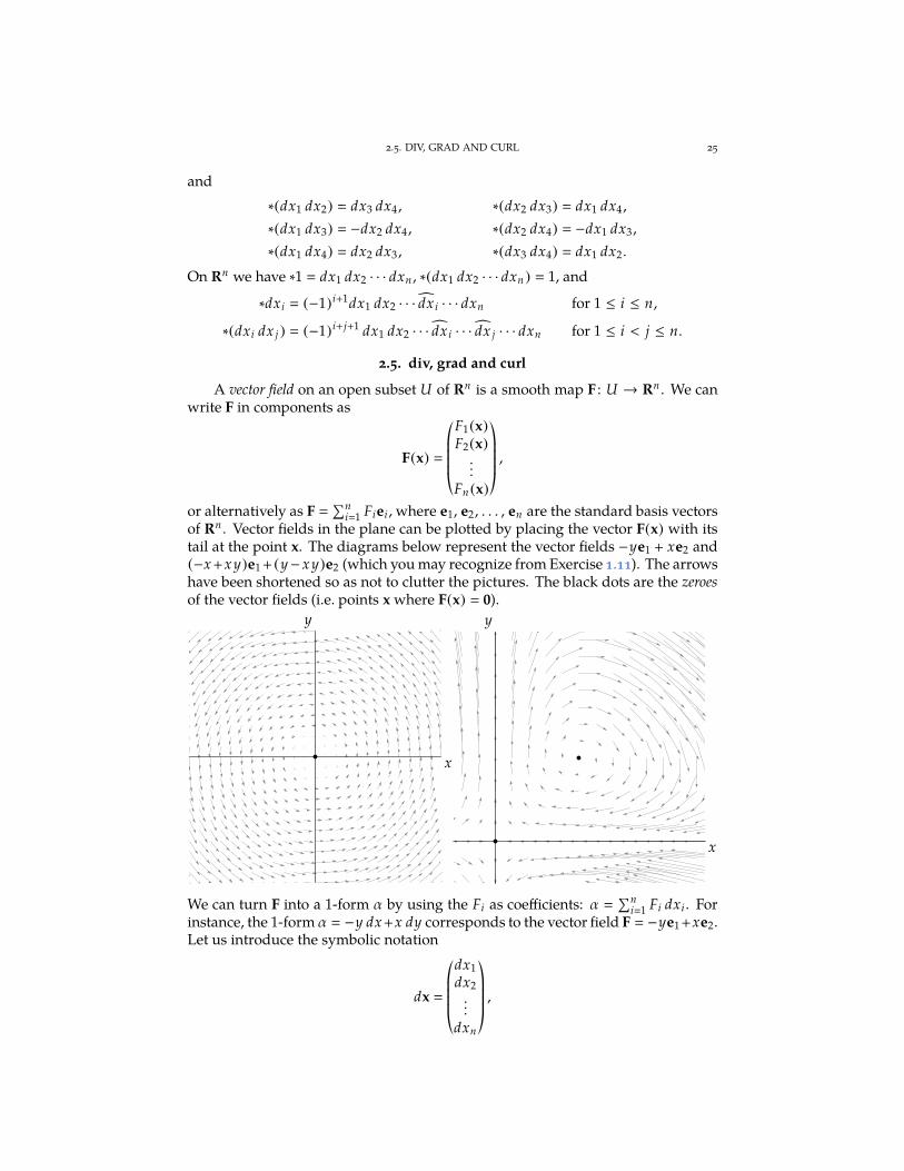
of Rn . Vector fields in the plane can be plotted by placing the vector F(x) with itstail at the point x. The diagrams below represent the vector fields −ye1 + xe2 and(−x +x y)e1 + (y−x y)e2 (which you may recognize from Exercise 1.11). The arrowshave been shortened so as not to clutter the pictures. The black dots are the zeroesof the vector fields (i.e. points x where F(x) 0).
x
y
x
y
We can turn F into a 1-form α by using the Fi as coefficients: α
∑ni1 Fi dxi . For
instance, the 1-form α −y dx +x dy corresponds to the vector field F −ye1 +xe2.Let us introduce the symbolic notation
dx
*....,
dx1
dx2
...dxn
+////-,
26 2. DIFFERENTIAL FORMS ON EUCLIDEAN SPACE
which we will think of as a vector-valued 1-form. Then we can write α F · dx.Clearly, F is determined by α and vice versa. Thus vector fields and 1-forms aresymbiotically associated to one another.
vector field F←→ 1-form α: α F · dx.
Intuitively, the vector-valued 1-form dx represents an infinitesimal displacement.If F represents a force field, such as gravity or electricity acting on a particle, thenα F · dx represents the work done by the force when the particle is displaced byan amount dx. (If the particle travels along a path, the total work done by the forceis found by integrating α along the path. We shall see how to do this in Section 4.1.)
The correspondence between vector fields and 1-forms behaves in an interest-ing way with respect to exterior differentiation and the Hodge star operator. Foreach function f the 1-form d f
∑ni1(∂ f /∂xi) dxi is associated to the vector field
grad( f )
n∑
i1
∂ f
∂xiei
*.......,
∂ f
∂x1∂ f
∂x2
...∂ f
∂xn
+///////-
.
This vector field is called the gradient of f . (Equivalently, we can view grad( f ) asthe transpose of the Jacobi matrix of f .)
grad( f )←→ d f : d f grad( f ) · dx.
Starting with a vector field F and letting α F · dx, we find
∗α
n∑
i1
Fi (∗dxi )
n∑
i1
Fi (−1)i+1 dx1 dx2 · · · dx i · · · dxn ,
Using the vector-valued n − 1-form
∗dx
*....,
∗dx1
∗dx2
...∗dxn
+////-
*....,
dx2 dx3 · · · dxn
−dx1 dx3 · · · dxn
...(−1)n+1dx1 dx2 · · · dxn−1
+////-
we can also write ∗α F·∗dx. Intuitively, the vector-valued n−1-form ∗dx representsan infinitesimal n − 1-dimensional hypersurface perpendicular to dx. (This pointof view will be justified in Section 8.3, after the proof of Theorem 8.16.) In fluidmechanics, the flow of a fluid or gas in Rn is represented by a vector field F. Then − 1-form ∗α then represents the flux, that is the amount of material passingthrough the hypersurface ∗dx per unit time. (The total amount of fluid passingthrough a hypersurface S is found by integrating α over S. We shall see how to dothis in Section 5.1.) We have
d∗α d(F · ∗dx)
n∑
i1
∂Fi
∂xi(−1)i+1 dxi dx1 dx2 · · · dx i · · · dxn
n∑
i1
∂Fi
∂xidx1 dx2 · · · dxi · · · dxn
( n∑
i1
∂Fi
∂xi
)
dx1 dx2 · · · dxn .
EXERCISES 27
The function div(F) ∑n
i1 ∂Fi/∂xi is the divergence of F. Thus if α F · dx, then
d∗α d(F · ∗dx) div(F) dx1 dx2 · · · dxn .
An alternative way of writing this identity is obtained by applying ∗ to both sides,which gives
div(F) ∗d∗α.
A very different identity is found by first applying d and then ∗ to α:
dα
n∑
i , j1
∂Fi
∂x jdx j dxi
∑
1≤i< j≤n
( ∂F j
∂xi− ∂Fi
∂x j
)
dxi dx j ,
and hence
∗dα
∑
1≤i< j≤n
(−1)i+ j+1( ∂F j
∂xi− ∂Fi
∂x j
)
dx1 dx2 · · · dx i · · · dx j · · · dxn .
In three dimensions ∗dα is a 1-form and so is associated to a vector field, namely
curl(F)
(∂F3
∂x2− ∂F2
∂x3
)
e1 −(∂F3
∂x1− ∂F1
∂x3
)
e2 +(∂F2
∂x1− ∂F1
∂x2
)
e3,
the curl of F. Thus, for n 3, if α F · dx, then
curl(F) · dx ∗dα.
You need not memorize every detail of this discussion. The point is rather toremember that exterior differentiation in combination with the Hodge star unifiesand extends to arbitrary dimensions the classical differential operators of vectorcalculus.
Exercises
2.1. Consider the forms α x dx − y dy, β z dx dy + x dy dz and γ z dy on R3.Calculate
(i) αβ, αβγ;(ii) dα, dβ, dγ.
2.2. Compute the exterior derivative of the following forms. Recall that a hat indicatesthat a term has to be omitted.
(i) ex y+z2dx.
(ii)∑n
i1x2
idx1 · · · dx i · · · dxn .
2.3. Calculate d sin f (x)2 , where f : Rn → R is an arbitrary smooth function.
2.4. Define functions ξ and η by
ξ(x, y) x
√
x2 + y2, η(x, y)
y√
x2 + y2.
Show that α0 −η dξ + ξ dη, where α0 denotes the angle form defined in Example 2.10.
2.5. Write the coordinates on R2n as (x1 , y1 , x2 , y2 , . . . , xn , yn ). Let
ω dx1 dy1 + dx2 dy2 + · · · + dxn dyn
n∑
i1
dxi dyi .
Compute ωn ωω · · ·ω (n-fold product). (First work out the cases n 1, 2, 3.)
28 2. DIFFERENTIAL FORMS ON EUCLIDEAN SPACE
2.6. Write the coordinates on R2n+1 as (x1 , y1 , x2 , y2 , . . . , xn , yn , z). Let
α dz + x1 dy1 + x2 dy2 + · · · + xn dyn dz +
n∑
i1
xi dyi .
Compute α(dα)n α(dα dα · · · dα). (Use the result of Exercise (2.5).)
2.7. Check that each of the following forms α ∈ Ω1(R3) is closed and find a function gsuch that dg α.
(i) α (yex y − z sin(xz)) dx + (xex y + z2) dy + (−x sin(xz) + 2yz + 3z2) dz.
(ii) α 2xy3z4 dx + (3x2 y2z4 − ze y sin(ze y )) dy + (4x2 y3z3 − e y sin(ze y ) + ez ) dz.
2.8. Let α
∑ni1
fi dxi be a closed 1-form on Rn . Define a function g by
g(x)
∫ x1
0f1(t , x2 , x3 , . . . , xn ) dt +
∫ x2
0f2(0, t , x3 , x4 , . . . , xn ) dt
+
∫ x3
0f3 (0, 0, t , x4 , x5 , . . . , xn ) dt + · · · +
∫ xn
0fn (0, 0, . . . , 0, t) dt.
Show that dg α. (Apply the fundamental theorem of calculus, formula (B.3), differentiateunder the integral sign and don’t forget to use dα 0. If you get confused, first do the case
n 2, where g(x) ∫ x1
0 f1(t , x2) dt +∫ x2
0 f2(0, t) dt.)
2.9. Let α
∑ni1
fi dxi be a closed 1-form whose coefficients fi are smooth functions
defined on Rn \ 0 that are all homogeneous of the same degree p , −1. Let
g(x) 1
p + 1
n∑
i1
xi fi (x).
Show that dg α. (Use dα 0 and apply the identity proved in Exercise B.6 to each fi .)
2.10. Let α and β be closed forms. Prove that αβ is also closed.
2.11. Let α be closed and β exact. Prove that αβ is exact.
2.12. Calculate ∗α, ∗β, ∗γ, ∗(αβ), where α, β and γ are as in Exercise 2.1.
2.13. Let α x1 dx2 + x3 dx4, β x1x2 dx3 dx4 + x3x4 dx1 dx2 and γ x2 dx1 dx3 dx4
be forms on R4. Calculate
(i) αβ, αγ;(ii) dβ, dγ;
(iii) ∗α, ∗γ.
2.14. Consider the form α −x22
dx1 + x21
dx2 on R2.
(i) Find ∗α and ∗d∗dα (where ∗d∗dα is shorthand for ∗(d(∗(dα))).)(ii) Repeat the calculation, regarding α as a form on R3.
(iii) Again repeat the calculation, now regarding α as a form on R4.
2.15. Prove that ∗∗α (−1)kn+kα for every k-form α on Rn .
2.16. Recall that for any increasing multi-index I (i1 , i2 , . . . , ik ) the number εI ±1is determined by the requirement that
dxI dxIc εI dx1 dx2 . . . dxn .
Let us define |I | i1 + i2 + · · · + ik . Show that εI (−1)|I |+
(k+12
)
.
EXERCISES 29
2.17. Let α
∑
I aI dxI and β
∑
J b J dx J be constant k-forms on Rn , i.e. forms withconstant coefficients aI and b J . (We also assume, as usual, that the multi-indices I and J areincreasing.) The inner product of α and β is the number defined by
(α, β) ∑
I
aI bI .
For instance, if α 7 dx1 dx2 +√
2 dx1 dx3 + 11 dx2 dx3 and β 5 dx1 dx3 − 3 dx2 dx3, then
(α, β) √
2 · 5 + 11 ·(−3) 5√
2 − 33.
Prove the following assertions.
(i) The dxI form an orthonormal basis of the space of constant k-forms.(ii) (α, α) ≥ 0 for all α and (α, α) 0 if and only if α 0.
(iii) α(∗β) (α, β) dx1 dx2 · · · dxn .(iv) α(∗β) β(∗α).(v) The Hodge star operator is orthogonal, i.e. (α, β) (∗α, ∗β).
2.18. The Laplacian ∆ f of a smooth function f on an open subset of Rn is defined by
∆ f
∂2 f
∂x21
+∂2 f
∂x22
+ · · · +∂2 f
∂x2n
.
Prove the following formulas.
(i) ∆ f ∗d∗d f .(ii) ∆( f g) (∆ f )g + f∆g + 2 ∗(d f (∗dg)). (Use Exercise 2.17(iv).)
2.19. Let α
∑ni1 fi dxi be a 1-form on Rn .
(i) Find formulas for ∗α, d∗α, ∗d∗α, and d∗d∗α.(ii) Find formulas for dα, ∗dα, d∗dα, and ∗d∗dα.
(iii) Finally compute d∗d∗α + (−1)n∗d∗dα. Try to write the answer in terms of theLaplace operator ∆ defined in Exercise 2.18.
2.20. Let α be the 1-form ‖x‖2px · ∗dx on Rn , where p is a real constant. Compute dα.
Show that α is closed if and only if p − 12 n.
2.21. (i) Let U be an open subset of Rn and let f : U → R be a function satisfyinggrad( f )(x) , 0 for all x in U. On U define a vector field n, an n − 1-form ν and a1-form α by
n(x) ‖grad( f )(x)‖−1 grad( f )(x),
ν n · ∗dx,
α ‖grad( f )(x)‖−1d f .
Prove that dx1 dx2 · · · dxn αν on U.(ii) Let r : Rn → R be the function r (x) ‖x‖ (distance to the origin). Deduce from
part (i) that dx1 dx2 · · · dxn (dr)ν on Rn \ 0, where ν ‖x‖−1x · ∗dx.
2.22. The Minkowski or relativistic inner product on Rn+1 is given by
(x, y)
n∑
i1
xi yi − xn+1 yn+1.
A vector x ∈ Rn+1 is spacelike if (x, x) > 0, lightlike if (x, x) 0, and timelike if (x, x) < 0.
(i) Give examples of (nonzero) vectors of each type.(ii) Show that for every x , 0 there is a y such that (x, y) , 0.
30 2. DIFFERENTIAL FORMS ON EUCLIDEAN SPACE
A Hodge star operator corresponding to this inner product is defined as follows: if α
∑
I fI dxI , then
∗α
∑
I
fI (∗dxI ),
with
∗dxI εI dxIc if I contains n + 1,
−εI dxIc if I does not contain n + 1.
(Here εI and Ic are as in the definition of the ordinary Hodge star.)
(iii) Find ∗1, ∗dxi for 1 ≤ i ≤ n + 1, and ∗(dx1 dx2 · · · dxn ).(iv) Compute the “relativistic Laplacian” (usually called the d’Alembertian or wave
operator) ∗d∗d f for any smooth function f on Rn+1.(v) For n 3 (ordinary space-time) find ∗(dxi dx j ) for 1 ≤ i < j ≤ 4.
2.23. One of the greatest advances in theoretical physics of the nineteenth century wasMaxwell’s formulation of the equations of electromagnetism:
curl(E) −1
c
∂B
∂t(Faraday’s Law),
curl(H) 4π
cJ +
1
c
∂D
∂t(Ampère’s Law),
div(D) 4πρ (Gauss’ Law),
div(B) 0 (no magnetic monopoles).
Here c is the speed of light, E is the electric field, H is the magnetic field, J is the densityof electric current, ρ is the density of electric charge, B is the magnetic induction and D is
the dielectric displacement. E, H, J, B and D are vector fields and ρ is a function on R3 andall depend on time t. The Maxwell equations look particularly simple in differential form
notation, as we shall now see. In space-time R4 with coordinates (x1 , x2 , x3 , x4), wherex4 ct, introduce forms
α (E1 dx1 + E2 dx2 + E3 dx3) dx4 + B1 dx2 dx3 + B2 dx3 dx1 + B3 dx1 dx2 ,
β −(H1 dx1 + H2 dx2 + H3 dx3) dx4 + D1 dx2 dx3 + D2 dx3 dx1 + D3 dx1 dx2 ,
γ
1
c( J1 dx2 dx3 + J2 dx3 dx1 + J3 dx1 dx2) dx4 − ρ dx1 dx2 dx3 .
(i) Show that Maxwell’s equations are equivalent to
dα 0,
dβ + 4πγ 0.
(ii) Conclude that γ is closed and that div(J) + ∂ρ/∂t 0.(iii) In vacuum one has E D and H B. Show that in vacuum β ∗α, the relativistic
Hodge star of α defined in Exercise 2.22.
(iv) Free space is a vacuum without charges or currents. Show that the Maxwellequations in free space are equivalent to dα d∗α 0.
(v) Let f , g : R→ R be any smooth functions and define
E(x) *.,
0f (x1 − x4)
g(x1 − x4)
+/-, B(x)
*.,
0−g(x1 − x4)
f (x1 − x4)
+/-.
Show that the corresponding 2-form α satisfies the free Maxwell equations dα
d∗α 0. Such solutions are called electromagnetic waves. Explain why. In whatdirection do these waves travel?
CHAPTER 3
Pulling back forms
3.1. Determinants
The determinant of a square matrix is the oriented volume of the parallelepipedspanned by its column vectors. It is therefore not surprising that differential formsare closely related to determinants. This section is a review of some fundamentalfacts concerning determinants.
Let
A
*..,
a1,1 . . . a1,n...
...an ,1 . . . an ,n
+//-
be an n × n-matrix with column vectors a1, a2, . . . , an . The parallelepiped spannedby the columns is by definition the set of all linear combinations
∑ni1 ciai , where
the coefficients ci range over the unit interval [0, 1]. A parallelepiped spanned bya single vector is called a line segment and a parallelepiped spanned by two vectorsis called a parallelogram. The determinant of A is variously denoted by
det(A) det(a1 , a2, . . . , an) det(ai , j )1≤i , j≤n
a1,1 . . . a1,n...
...an ,1 . . . an ,n
.
Expansion on the j-th column. You may have seen the following definition ofthe determinant:
det(A)
n∑
i1
(−1)i+1ai , j det(Ai , j ).
Here Ai , j denotes the (n − 1) × (n − 1)-matrix obtained from A by crossing outthe i-th row and the j-th column. This is a recursive definition, which reducesthe calculation of any determinant to that of determinants of smaller size. Therecursion starts at n 1; the determinant of a 1 × 1-matrix (a) is simply defined tobe the number a. It is a useful rule, but it has two serious flaws: first, it is extremelyinefficient computationally (except for matrices containing lots of zeroes), andsecond, it obscures the relationship with volumes of parallelepipeds.
Axioms. A far better definition is available. The determinant can be com-pletely characterized by a few simple axioms, which make good sense in view ofits geometrical significance and which comprise an efficient algorithm for calcu-lating any determinant. To motivate these axioms we first consider the case of a2 × 2-matrix A (n 2). Then the columns a1 and a2 are vectors in the plane, andinstead of the oriented “volume” we speak of the oriented area of the parallelogram
spanned by a1 and a2. (This notion is familiar from calculus: the integral∫ b
a f (x) dx
31
32 3. PULLING BACK FORMS
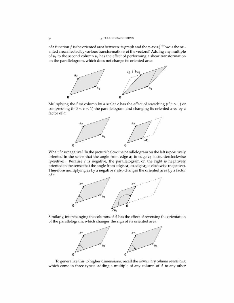
of a function f is the oriented area between its graph and the x-axis.) How is the ori-ented area affected by various transformations of the vectors? Adding any multipleof a1 to the second column a2 has the effect of performing a shear transformationon the parallelogram, which does not change its oriented area:
a1
a2
0
a1
a2 + ba1
0
Multiplying the first column by a scalar c has the effect of stretching (if c > 1) orcompressing (if 0 < c < 1) the parallelogram and changing its oriented area by afactor of c:
a1
a2
0
ca1
a2
0
What if c is negative? In the picture below the parallelogram on the left is positivelyoriented in the sense that the angle from edge a1 to edge a2 is counterclockwise(positive). Because c is negative, the parallelogram on the right is negativelyoriented in the sense that the angle from edge ca1 to edge a2 is clockwise (negative).Therefore multiplying a1 by a negative c also changes the oriented area by a factorof c:
a1
a2
0ca1
a2
0
Similarly, interchanging the columns of A has the effect of reversing the orientationof the parallelogram, which changes the sign of its oriented area:
a1
a2
0
a1
a2
0
To generalize this to higher dimensions, recall the elementary column operations,which come in three types: adding a multiple of any column of A to any other
3.1. DETERMINANTS 33
column (type I); multiplying a column by a nonzero constant (type II); and inter-changing any two columns (type III). As suggested by the pictures above, type Idoes not affect the determinant, type II multiplies it by the corresponding constant,and type III causes a sign change. We turn these observations into a definition asfollows.
3.1. Definition. A determinant is a function det which assigns to every n × n-matrix A a number det(A) subject to the following axioms:
(i) If E is an elementary column operation, then det(E(A)) k det(A),where
k
1 if E is of type I,c if E is of type II (multiplication of a column by c),−1 if E is of type III.
(ii) det(I) 1.
Axiom (ii) is a normalization convention, which is justified by the reasonablerequirement that the unit cube in Rn (i.e. the parallelepiped spanned by the columnsof the identity matrix I) should have oriented volume 1.
3.2. Example. The following calculation is a sequence of column operations, atthe end of which we apply the normalization axiom.
1 1 14 10 91 5 4
1 0 04 6 51 4 3
1 0 04 1 51 1 3
1 0 03 1 20 1 0
2
1 0 03 1 10 1 0
2
1 0 00 0 10 1 0
−2
1 0 00 1 00 0 1
−2.
As this example suggests, the axioms of Definition 3.1 suffice to calculate anyn × n-determinant. In other words, there is at most one function det which obeysthese axioms. More precisely, we have the following result.
3.3. Theorem (uniqueness of determinants). Let det and det′ be two functionssatisfying Axioms (i)–(ii). Then det(A) det′(A) for all n × n-matrices A.
Proof. Let a1, a2, . . . , an be the column vectors of A. Suppose first that Ais not invertible. Then the columns of A are linearly dependent. For simplicitylet us assume that the first column is a linear combination of the others: a1
c2a2 + · · · + cnan . Repeatedly applying type I column operations gives
det(A) det( n∑
i2
ciai , a2, . . . , ai , . . . , an
)
det(0, a2, . . . , ai , . . . , an).
Applying a type II operation gives
det(0, a2, . . . , ai , . . . , an) det(−0, a2, . . . , ai , . . . , an)
−det(0, a2, . . . , ai , . . . , an),
and therefore det(A) 0. For the same reason det′(A) 0, so det(A) det′(A).Now assume that A is invertible. Then A is column equivalent to the identity
34 3. PULLING BACK FORMS
matrix, i.e. it can be transformed to I by successive elementary column operations.Let E1, E2, . . . , Em be these elementary operations, so that EmEm−1 · · ·E2E1(A) I.By Axiom (i) each operation Ei has the effect of multiplying the determinant by acertain factor ki , so Axiom (ii) yields
1 det(I) det(EmEm−1 · · ·E2E1(A)) km km−1 · · · k2k1 det(A).
Applying the same reasoning to det′(A) we get 1 km km−1 · · · k2k1 det′(A). Hencedet(A) 1/(k1k2 · · · km ) det′(A). QED
3.4. Remark (change of normalization). Suppose that det′ is a function thatsatisfies Axiom (i) but is normalized differently: det′(I) c. Then the proof ofTheorem 3.3 shows that det′(A) c det(A) for all n × n-matrices A.
The counterpart of this uniqueness theorem is an existence theorem, whichstates that Axioms 3.1(i)–(ii) are consistent. We will establish consistence by dis-playing an explicit formula for the determinant of any n × n-matrix that does notinvolve any column reductions. Unlike Definition 3.1, this formula is not verypractical for the purpose of calculating large determinants, but it has other uses,notably in the theory of differential forms.
3.5. Theorem (existence of determinants). Every n×n-matrix A has a well-defineddeterminant. It is given by the formula
det(A) ∑
σ∈Sn
sign(σ)a1,σ(1) a2,σ(2) · · · an ,σ(n) .
This requires a little explanation. Sn stands for the collection of all permutationsof the set 1, 2, . . . , n. A permutation is a way of ordering the numbers 1, 2, . . . ,n. Permutations are usually written as n-tuples containing each of these numbersexactly once. Thus for n 2 there are only two permutations: (1, 2) and (2, 1). Forn 3 all possible permutations are
(1, 2, 3), (1, 3, 2), (2, 1, 3), (2, 3, 1), (3, 1, 2), (3, 2, 1).
For general n there are
n(n − 1)(n − 2) · · · 3 · 2 · 1 n!
permutations. An alternative way of thinking of a permutation is as a bijective (i.e.one-to-one and onto) map from the set 1, 2, . . . , n to itself. For example, for n 5a possible permutation is
(5, 3, 1, 2, 4),
and we think of this as a shorthand notation for the map σ given by σ(1) 5,σ(2) 3, σ(3) 1, σ(4) 2 and σ(5) 4. The permutation (1, 2, 3, . . . , n − 1, n)
then corresponds to the identity map of the set 1, 2, . . . , n.If σ is the identity permutation, then clearly σ(i) < σ( j) whenever i < j.
However, if σ is not the identity permutation, it cannot preserve the order in thisway. An inversion of σ is any pair of numbers i and j such that 1 ≤ i < j ≤ n andσ(i) > σ( j). The length of σ, denoted by l(σ), is the number of inversions of σ. Apermutation is called even or odd according to whether its length is even, resp. odd.
3.1. DETERMINANTS 35
For instance, the permutation (5, 3, 1, 2, 4) has length 6 and so is even. The sign ofσ is
sign(σ) (−1)l(σ)
1 if σ is even,−1 if σ is odd.
Thus sign(5, 3, 1, 2, 4) 1. The permutations of 1, 2 are (1, 2), which has sign 1,and (2, 1), which has sign −1, while for n 3 we have the table below.
σ l(σ) sign(σ)
(1, 2, 3) 0 1(1, 3, 2) 1 −1(2, 1, 3) 1 −1(2, 3, 1) 2 1(3, 1, 2) 2 1(3, 2, 1) 3 −1
Thinking of permutations in Sn as bijective maps from 1, 2, . . . , n to itself,we can form the composition σ τ of any two permutations σ and τ in Sn . Forpermutations we usually write as στ instead of σ τ and call it the product of σ andτ. This is the permutation produced by first performing τ and then σ! For instance,if σ (5, 3, 1, 2, 4) and τ (5, 4, 3, 2, 1), then
τσ (1, 3, 5, 4, 2), στ (4, 2, 1, 3, 5).
A basic fact concerning signs, which we shall not prove here, is
sign(στ) sign(σ) sign(τ). (3.1)
In particular, the product of two even permutations is even and the product of aneven and an odd permutation is odd.
The determinant formula in Theorem 3.5 contains n! terms, one for each per-mutation σ. Each term is a product which contains exactly one entry from eachrow and each column of A. For instance, for n 5 the permutation (5, 3, 1, 2, 4)
contributes the term a1,5a2,3a3,1a4,2a5,4. For 2× 2- and 3× 3-determinants Theorem3.5 gives the well-known formulæ
a1,1 a1,2
a2,1 a2,2
a1,1a2,2 − a1,2a2,1 ,
a1,1 a1,2 a1,3
a2,1 a2,2 a2,3
a3,1 a3,2 a3,3
a1,1a2,2a3,3 − a1,1a2,3a3,2 − a1,2a2,1a3,3 + a1,2a2,3a3,1
+ a1,3a2,1a3,2 − a1,3a2,2a3,1 .
Proof of Theorem 3.5. We need to check that the right-hand side of the deter-minant formula in Theorem 3.5 obeys Axioms (i)–(ii) of Definition 3.1. Let us forthe moment denote the right-hand side by f (A). Axiom (ii) is the easiest to verify:if A I, then
a1,σ(1) a2,σ(2) · · · an ,σ(n)
1 if σ identity,0 otherwise,
36 3. PULLING BACK FORMS
and therefore f (I) 1. Next we consider how f (A) behaves when we interchangetwo columns of A. We assert that each term in f (A) changes sign. To see this, let τbe the permutation in Sn that interchanges the two numbers i and j and leaves allothers fixed. Then
f (a1 , . . . , a j , . . . , ai , . . . , an)
∑
σ∈Sn
sign(σ)a1,τσ(1) a2,τσ(2) · · · an ,τσ(n)
∑
ρ∈Sn
sign(τρ)a1,ρ(1) a2,ρ(2) · · · an ,ρ(n) substitute ρ τσ
∑
ρ∈Sn
sign(τ) sign(ρ)a1,ρ(1) a2,ρ(2) · · · an ,ρ(n) by formula (3.1)
−∑
ρ∈Sn
sign(ρ)a1,ρ(1) a2,ρ(2) · · · an ,ρ(n) by Exercise 3.5
− f (a1, . . . , ai , . . . , a j , . . . , an).
To see what happens when we multiply a column of A by c, observe that for everypermutation σ the product
a1,σ(1) a2,σ(2) · · · an ,σ(n)
contains exactly one entry from each row and each column in A. So if we multiplythe i-th column of A by c, each term in f (A) is multiplied by c. Therefore
f (a1 , a2, . . . , cai , . . . , an) c f (a1 , a2, . . . , ai , . . . , an).
By a similar argument we have
f (a1 , a2, . . . , ai + a′i , . . . , an) f (a1 , a2, . . . , ai , . . . , an) + f (a1, a2, . . . , a′i , . . . , an)
for any vector a′i. In particular we can take a′
i a j for some j , i, which gives
f (a1 , a2, . . . , ai + a j , . . . , a j , . . . , an) f (a1 , a2, . . . , ai , . . . , a j , . . . , an)
+ f (a1 , a2, . . . , a j , . . . , a j , . . . , an)
f (a1 , a2, . . . , ai , . . . , a j , . . . , an),
because f (a1 , a2, . . . , ai , . . . , a j , . . . , an) 0. This shows that f satisfies the condi-tions of Definition 3.1. QED
We can calculate the determinant of any matrix by column reducing it to theidentity matrix, but there are many different ways of performing this reduction.Theorem 3.5 implies that different column reductions lead to the same answer forthe determinant.
The following corollary of Theorem 3.5 amounts to a reformulation of Defini-tion 3.1. Recall that e1, e2, . . . , en denote the standard basis vectors of Rn , i.e. thecolumns of the identity n × n-matrix.
3.6. Corollary. The determinant possesses the following properties. These propertiescharacterize the determinant uniquely.
(i) det is multilinear (i.e. linear in each column):
det(a1, a2, . . . , cai + c′a′i , . . . , an)
c det(a1 , a2, . . . , ai , . . . , an) + c′ det(a1 , a2, . . . , a′i , . . . , an)
3.1. DETERMINANTS 37
for all scalars c, c′ and all vectors a1, a2, . . . , ai, a′i, . . . , an ;
(ii) det is alternating (or antisymmetric):
det(a1, . . . , ai , . . . , a j , . . . , an) −det(a1 , . . . , a j , . . . , ai , . . . , an)
for all vectors a1, a2, . . . , an and for all pairs of distinct indices i , j;(iii) normalization: det(e1, e2, . . . , en) 1.
Proof. Property (i) was established in the proof of Theorem 3.5, while prop-erties (ii)–(iii) are simply a restatement of part of Definition 3.1. Therefore thedeterminant has properties (i)–(iii). Conversely, properties (i)–(iii) taken togetherimply Axioms (i)–(ii) of Definition 3.1. Therefore, by Theorem 3.3, properties(i)–(iii) characterize the determinant uniquely. QED
Here are some further rules obeyed by determinants. Each can be deducedfrom Definition 3.1 or from Theorem 3.5. (Recall that the transpose of an n×n-matrixA (ai , j ) is the matrix AT whose i, j-th entry is a j,i .)
3.7. Theorem. Let A and B be n × n-matrices.
(i) det(A) a1,1a2,2 · · · an ,n if A is upper triangular (i.e. ai , j 0 for i > j).(ii) det(AB) det(A) det(B).
(iii) det(AT ) det(A).(iv) (Expansion on the j-th column) det(A)
∑ni1(−1)i+ j ai , j det(Ai , j ) for all
j 1, 2, . . . , n. Here Ai , j denotes the (n − 1) × (n − 1)-matrix obtained fromA by deleting the i-th row and the j-th column.
(v) Let σ ∈ Sn be a permutation. Then
det(
aσ(1) , aσ(2) , . . . , aσ(n)
)
sign(σ) det(a1, a2, . . . , an).
When calculating determinants in practice one combines column reductionswith these rules. For instance, rule (i) tells us we need not bother reducing Aall the way to the identity matrix, like we did in Example 3.2, but that an uppertriangular form suffices. Rule (iii) tells us we may use row operations as well ascolumn operations.
Volume change. We conclude this discussion with a slightly different geo-metric view of determinants. A square matrix A can be regarded as a linear mapA : Rn → Rn . The unit cube in Rn ,
[0, 1]n x ∈ Rn | 0 ≤ xi ≤ 1 for i 1, 2, . . . , n ,
has n-dimensional volume 1. (For n 1 it is usually called the unit interval and forn 2 the unit square.) Its image A
(
[0, 1]n) under the map A is the parallelepipedspanned by the vectors Ae1, Ae2, . . . , Aen, which are the columns of A. HenceA
(
[0, 1]n) has n-dimensional volume
vol(
A([0, 1]n))
|det(A| |det(A) | vol([0, 1]n).
38 3. PULLING BACK FORMS
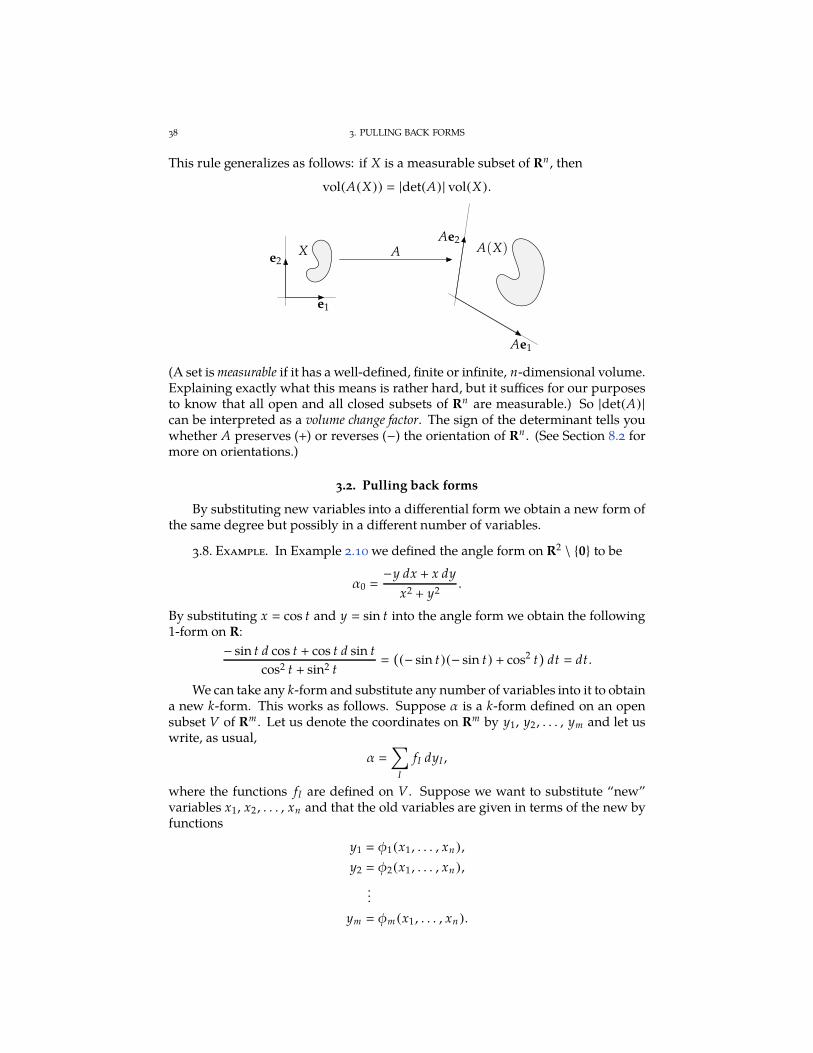
This rule generalizes as follows: if X is a measurable subset of Rn , then
vol(A(X)) |det(A) | vol(X).
X
e1
e2A A(X)
Ae1
Ae2
(A set is measurable if it has a well-defined, finite or infinite, n-dimensional volume.Explaining exactly what this means is rather hard, but it suffices for our purposesto know that all open and all closed subsets of Rn are measurable.) So |det(A) |can be interpreted as a volume change factor. The sign of the determinant tells youwhether A preserves (+) or reverses (−) the orientation of Rn . (See Section 8.2 formore on orientations.)
3.2. Pulling back forms
By substituting new variables into a differential form we obtain a new form ofthe same degree but possibly in a different number of variables.
3.8. Example. In Example 2.10 we defined the angle form on R2 \ 0 to be
α0
−y dx + x dy
x2 + y2.
By substituting x cos t and y sin t into the angle form we obtain the following1-form on R:
− sin t d cos t + cos t d sin t
cos2 t + sin2 t
(
(− sin t)(− sin t) + cos2 t)
dt dt .
We can take any k-form and substitute any number of variables into it to obtaina new k-form. This works as follows. Suppose α is a k-form defined on an opensubset V of Rm . Let us denote the coordinates on Rm by y1, y2 , . . . , ym and let uswrite, as usual,
α
∑
I
fI dyI ,
where the functions fI are defined on V. Suppose we want to substitute “new”variables x1, x2 , . . . , xn and that the old variables are given in terms of the new byfunctions
y1 φ1(x1 , . . . , xn ),
y2 φ2(x1 , . . . , xn ),
...
ym φm (x1 , . . . , xn ).
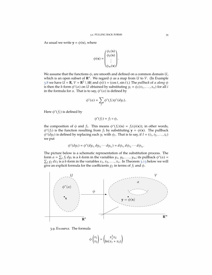
3.2. PULLING BACK FORMS 39
As usual we write y φ(x), where
φ(x)
*....,
φ1(x)
φ2(x)...
φm (x)
+////-.
We assume that the functions φi are smooth and defined on a common domain U ,which is an open subset of Rn . We regard φ as a map from U to V. (In Example3.8 we have U R, V R2 \ 0 and φ(t) (cos t , sin t).) The pullback of α along φis then the k-form φ∗(α) on U obtained by substituting yi φi (x1 , . . . , xn ) for all iin the formula for α. That is to say, φ∗(α) is defined by
φ∗(α) ∑
I
φ∗( fI )φ∗(dyI ).
Here φ∗( fI ) is defined by
φ∗( fI ) fI φ,
the composition of φ and fI . This means φ∗( fI )(x) fI (φ(x)); in other words,φ∗( fI ) is the function resulting from fI by substituting y φ(x). The pullbackφ∗(dyI ) is defined by replacing each yi with φi . That is to say, if I (i1 , i2 , . . . , ik )
we put
φ∗(dyI ) φ∗(dyi1 dyi2 · · · dyik ) dφi1 dφi2 · · · dφik .
The picture below is a schematic representation of the substitution process. Theform α
∑
I fI dyI is a k-form in the variables y1, y2 , . . . , ym ; its pullback φ∗(α) ∑
J g J dx J is a k-form in the variables x1, x2 , . . . , xn . In Theorem 3.13 below we willgive an explicit formula for the coefficients g J in terms of fI and φ.
U V
Rn Rm
φφ∗(α)
α
x y = φ(x)
3.9. Example. The formula
φ
(
x1
x2
)
(
x31x2
ln(x1 + x2)
)
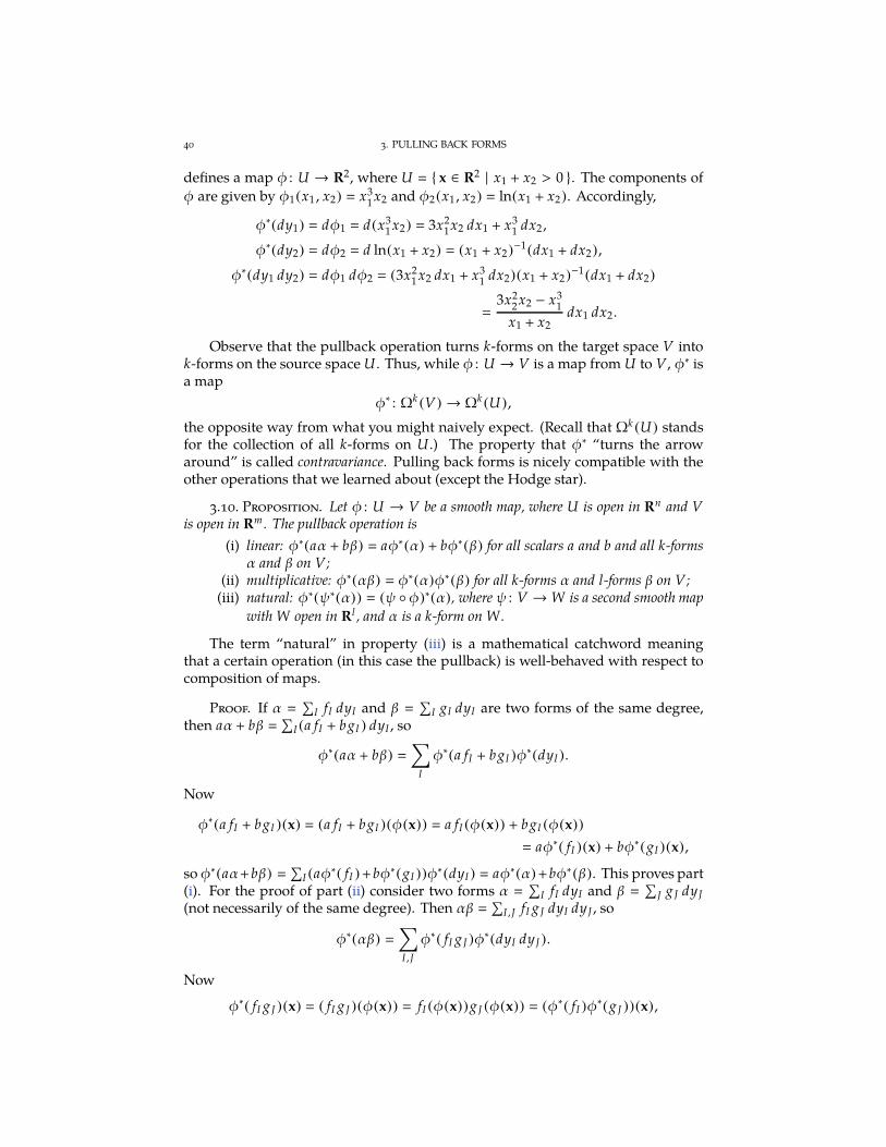
40 3. PULLING BACK FORMS
defines a map φ : U → R2, where U x ∈ R2 | x1 + x2 > 0 . The components ofφ are given by φ1(x1 , x2) x3
1x2 and φ2(x1 , x2) ln(x1 + x2). Accordingly,
φ∗(dy1) dφ1 d(x31x2) 3x2
1x2 dx1 + x31 dx2 ,
φ∗(dy2) dφ2 d ln(x1 + x2) (x1 + x2)−1(dx1 + dx2),
φ∗(dy1 dy2) dφ1 dφ2 (3x21x2 dx1 + x3
1 dx2)(x1 + x2)−1(dx1 + dx2)
3x22x2 − x3
1
x1 + x2dx1 dx2.
Observe that the pullback operation turns k-forms on the target space V intok-forms on the source space U . Thus, while φ : U → V is a map from U to V, φ∗ isa map
φ∗ : Ωk (V) → Ωk (U),
the opposite way from what you might naively expect. (Recall that Ωk (U) standsfor the collection of all k-forms on U .) The property that φ∗ “turns the arrowaround” is called contravariance. Pulling back forms is nicely compatible with theother operations that we learned about (except the Hodge star).
3.10. Proposition. Let φ : U → V be a smooth map, where U is open in Rn and Vis open in Rm . The pullback operation is
(i) linear: φ∗(aα + bβ) aφ∗(α) + bφ∗(β) for all scalars a and b and all k-formsα and β on V;
(ii) multiplicative: φ∗(αβ) φ∗(α)φ∗ (β) for all k-forms α and l-forms β on V;(iii) natural: φ∗(ψ∗(α)) (ψ φ)∗(α), where ψ : V →W is a second smooth map
with W open in Rl , and α is a k-form on W .
The term “natural” in property (iii) is a mathematical catchword meaningthat a certain operation (in this case the pullback) is well-behaved with respect tocomposition of maps.
Proof. If α
∑
I fI dyI and β
∑
I gI dyI are two forms of the same degree,then aα + bβ
∑
I (a fI + bgI ) dyI , so
φ∗(aα + bβ) ∑
I
φ∗(a fI + bgI )φ∗(dyI ).
Now
φ∗(a fI + bgI )(x) (a fI + bgI )(φ(x)) a fI (φ(x)) + bgI (φ(x))
aφ∗( fI )(x) + bφ∗(gI )(x),
so φ∗(aα+ bβ)
∑
I (aφ∗( fI ) + bφ∗(gI ))φ∗(dyI ) aφ∗(α) + bφ∗ (β). This proves part(i). For the proof of part (ii) consider two forms α
∑
I fI dyI and β
∑
J g J dy J
(not necessarily of the same degree). Then αβ
∑
I ,J fI g J dyI dy J , so
φ∗(αβ)
∑
I ,J
φ∗( fI g J )φ∗(dyI dy J ).
Now
φ∗( fI g J )(x) ( fI g J )(φ(x)) fI (φ(x))g J (φ(x)) (φ∗( fI )φ∗(g J ))(x),
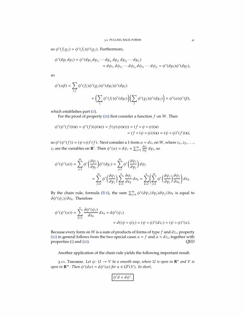
3.2. PULLING BACK FORMS 41
so φ∗( fI g J ) φ∗( fI )φ∗(g J ). Furthermore,
φ∗(dyI dy J ) φ∗(dyi1 dyi2 · · · dyik dy j1 dy j2 · · · dy jl )
dφi1 dφi2 · · · dφik dφ j1 · · · dφ jl φ∗(dyI )φ
∗(dy J ),
so
φ∗(αβ) ∑
I ,J
φ∗( fI )φ∗(g J )φ∗(dyI )φ
∗(dy J )
(∑
I
φ∗( fI )φ∗(dyI )
) (∑
I
φ∗(g J )φ∗(dy J )
)
φ∗(α)φ∗ (β),
which establishes part (ii).For the proof of property (iii) first consider a function f on W . Then
φ∗(ψ∗( f ))(x) ψ∗( f )(φ(x)) f (ψ(φ(x))) ( f ψ φ)(x)
( f (ψ φ))(x) (ψ φ)∗( f )(x),
so φ∗(ψ∗( f )) (ψφ)∗( f ). Next consider a 1-form α dzi on W , where z1, z2 , . . . ,
zl are the variables on Rl. Then ψ∗(α) dψi ∑m
j1∂ψi
∂y jdy j, so
φ∗(ψ∗(α))
m∑
j1
φ∗( ∂ψi
∂y j
)
φ∗(dy j)
m∑
j1
φ∗( ∂ψi
∂y j
)
dφ j
m∑
j1
φ∗( ∂ψi
∂y j
) n∑
k1
∂φ j
∂xkdxk
n∑
k1
( m∑
j1
φ∗( ∂ψi
∂y j
) ∂φ j
∂xk
)
dxk .
By the chain rule, formula (B.6), the sum∑m
j1 φ∗(∂ψi/∂y j)∂φ j/∂xk is equal to
∂φ∗(ψi )/∂xk. Therefore
φ∗(ψ∗(α))
n∑
k1
∂φ∗(ψi )
∂xkdxk dφ∗(ψi )
d((ψ φ)i ) (ψ φ)∗(dzi ) (ψ φ)∗(α).
Because every form on W is a sum of products of forms of type f and dzi , property(iii) in general follows from the two special cases α f and α dzi , together withproperties (i) and (iii). QED
Another application of the chain rule yields the following important result.
3.11. Theorem. Let φ : U → V be a smooth map, where U is open in Rn and V is
open in Rm . Then φ∗(dα) dφ∗(α) for α ∈ Ωk (V). In short,
φ∗d dφ∗ .
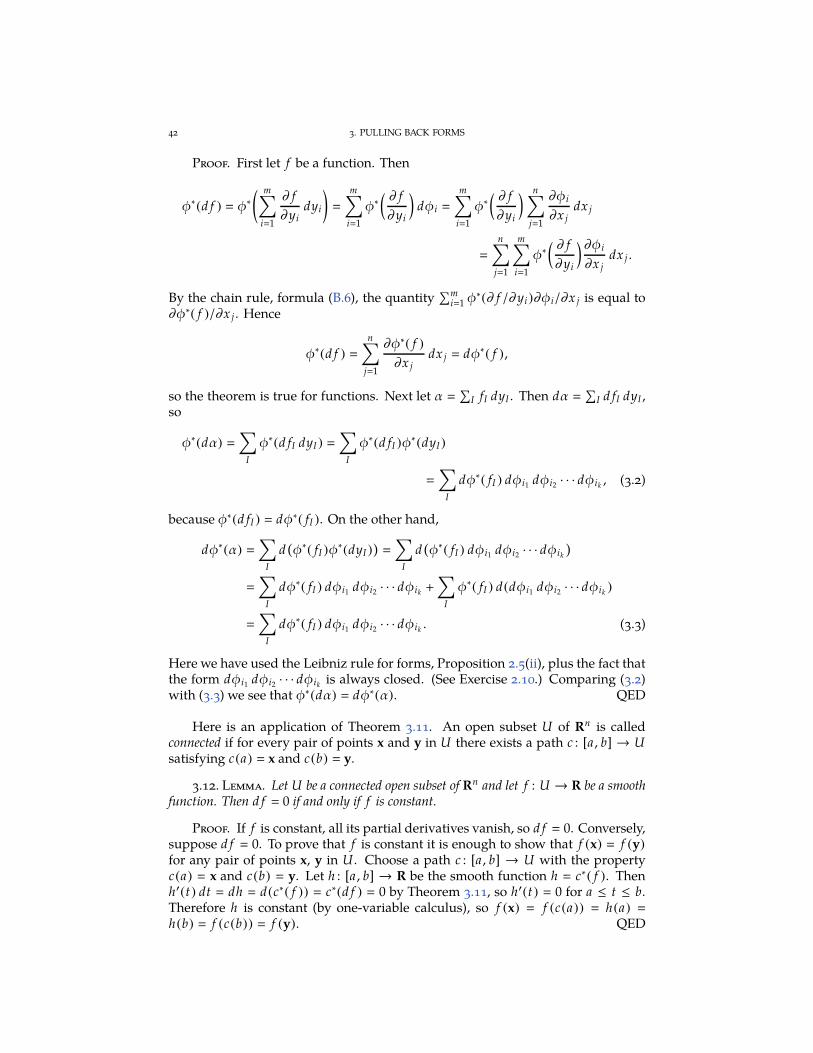
42 3. PULLING BACK FORMS
Proof. First let f be a function. Then
φ∗(d f ) φ∗( m∑
i1
∂ f
∂yidyi
)
m∑
i1
φ∗( ∂ f
∂yi
)
dφi
m∑
i1
φ∗( ∂ f
∂yi
) n∑
j1
∂φi
∂x jdx j
n∑
j1
m∑
i1
φ∗( ∂ f
∂yi
) ∂φi
∂x jdx j .
By the chain rule, formula (B.6), the quantity∑m
i1 φ∗(∂ f /∂yi)∂φi/∂x j is equal to
∂φ∗( f )/∂x j . Hence
φ∗(d f )
n∑
j1
∂φ∗( f )
∂x jdx j dφ∗( f ),
so the theorem is true for functions. Next let α
∑
I fI dyI . Then dα
∑
I d fI dyI ,so
φ∗(dα) ∑
I
φ∗(d fI dyI ) ∑
I
φ∗(d fI )φ∗(dyI )
∑
I
dφ∗( fI ) dφi1 dφi2 · · · dφik , (3.2)
because φ∗(d fI ) dφ∗( fI ). On the other hand,
dφ∗(α) ∑
I
d(
φ∗( fI )φ∗(dyI )
)
∑
I
d(
φ∗( fI ) dφi1 dφi2 · · · dφik
)
∑
I
dφ∗( fI ) dφi1 dφi2 · · · dφik +∑
I
φ∗( fI ) d(dφi1 dφi2 · · · dφik )
∑
I
dφ∗( fI ) dφi1 dφi2 · · · dφik . (3.3)
Here we have used the Leibniz rule for forms, Proposition 2.5(ii), plus the fact thatthe form dφi1 dφi2 · · · dφik is always closed. (See Exercise 2.10.) Comparing (3.2)with (3.3) we see that φ∗(dα) dφ∗(α). QED
Here is an application of Theorem 3.11. An open subset U of Rn is calledconnected if for every pair of points x and y in U there exists a path c : [a, b] → Usatisfying c(a) x and c(b) y.
3.12. Lemma. Let U be a connected open subset of Rn and let f : U → R be a smoothfunction. Then d f 0 if and only if f is constant.
Proof. If f is constant, all its partial derivatives vanish, so d f 0. Conversely,suppose d f 0. To prove that f is constant it is enough to show that f (x) f (y)
for any pair of points x, y in U . Choose a path c : [a, b] → U with the propertyc(a) x and c(b) y. Let h : [a, b] → R be the smooth function h c∗( f ). Thenh′(t) dt dh d(c∗( f )) c∗(d f ) 0 by Theorem 3.11, so h′(t) 0 for a ≤ t ≤ b.Therefore h is constant (by one-variable calculus), so f (x) f (c(a)) h(a)
h(b) f (c(b)) f (y). QED
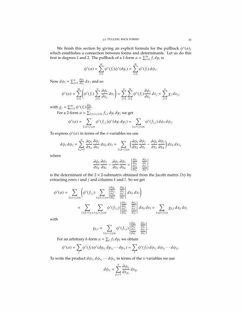
3.2. PULLING BACK FORMS 43
We finish this section by giving an explicit formula for the pullback φ∗(α),which establishes a connection between forms and determinants. Let us do thisfirst in degrees 1 and 2. The pullback of a 1-form α
∑mi1 fi dyi is
φ∗(α)
m∑
i1
φ∗( fi )φ∗(dyi )
m∑
i1
φ∗( fi ) dφi .
Now dφi ∑n
j1∂φi
∂x jdx j and so
φ∗(α)
m∑
i1
(
φ∗( fi )
n∑
j1
∂φi
∂x jdx j
)
n∑
j1
m∑
i1
φ∗( fi )∂φi
∂x jdx j
n∑
j1
g j dx j ,
with g j ∑m
i1 φ∗( fi )
∂φi
∂x j.
For a 2-form α
∑
1≤i< j≤m fi , j dyi dy j we get
φ∗(α) ∑
1≤i< j≤m
φ∗( fi , j )φ∗(dyi dy j )
∑
1≤i< j≤m
φ∗( fi , j ) dφi dφ j .
To express φ∗(α) in terms of the x-variables we use
dφi dφ j
n∑
k ,l1
∂φi
∂xk
∂φ j
∂xldxk dxl
∑
1≤k<l≤n
( ∂φi
∂xk
∂φ j
∂xl−∂φi
∂xl
∂φ j
∂xk
)
dxk dxl ,
where
∂φi
∂xk
∂φ j
∂xl−∂φi
∂xl
∂φ j
∂xk
∂φi
∂xk
∂φi
∂xl∂φ j
∂xk
∂φ j
∂xl
is the determinant of the 2 × 2-submatrix obtained from the Jacobi matrix Dφ byextracting rows i and j and columns k and l. So we get
φ∗(α) ∑
1≤i< j≤m
(
φ∗( fi , j )∑
1≤k<l≤n
∂φi
∂xk
∂φi
∂xl∂φ j
∂xk
∂φ j
∂xl
dxk dxl
)
∑
1≤k<l≤n
∑
1≤i< j≤m
φ∗( fi , j )
∂φi
∂xk
∂φi
∂xl∂φ j
∂xk
∂φ j
∂xl
dxk dxl
∑
1≤k<l≤n
gk ,l dxk dxl
with
gk ,l
∑
1≤i< j≤m
φ∗( fi , j )
∂φi
∂xk
∂φi
∂xl∂φ j
∂xk
∂φ j
∂xl
.
For an arbitrary k-form α
∑
I fI dyI we obtain
φ∗(α) ∑
I
φ∗( fI )φ∗(dyi1 dyi2 · · · dyik )
∑
I
φ∗( fI ) dφi1 dφi2 · · · dφik .
To write the product dφi1 dφi2 · · · dφik in terms of the x-variables we use
dφil
n∑
pl1
∂φil
∂xpl
dxpl
44 3. PULLING BACK FORMS
for l 1, 2, . . . , k. This gives
dφi1 dφi2 · · · dφik
n∑
p1 ,p2 ,...,pk1
∂φi1
∂xp1
∂φi2
∂xp2
· · ·∂φik
∂xpk
dxp1 dxp2 · · · dxpk
∑
P
∂φi1
∂xp1
∂φi2
∂xp2
· · ·∂φik
∂xpk
dxP ,
in which the summation is over all nk multi-indices P (p1 , p2 , . . . , pk ). If a multi-index P has repeating entries, then dxP 0. If the entries of P are all distinct, we canrearrange them in increasing order by means of a permutation σ. In other words,we have P (p1 , p2 , . . . , pk ) ( jσ(1) , jσ(2) , . . . , jσ(k)), where J ( j1 , j2, . . . , jk ) is anincreasing multi-index and σ ∈ Sk is a permutation. Thus we can rewrite the sumover all multi-indices P as a double sum over all increasing multi-indices J and allpermutations σ:
dφi1 dφi1 · · · dφik
∑
J
∑
σ∈Sk
∂φi1
∂x jσ(1)
∂φi2
∂x jσ(2)
· · ·∂φik
∂x jσ(k)
dx jσ(1)dx jσ(2)
· · · dx jσ(k)
∑
J
∑
σ∈Sk
sign(σ)∂φi1
∂x jσ(1)
∂φi2
∂x jσ(2)
· · ·∂φik
∂x jσ(k)
dx J (3.4)
∑
J
det(DφI ,J ) dx J . (3.5)
In (3.4) we used the result of Exercise 3.8 and in (3.5) we applied Theorem 3.5.The notation DφI ,J stands for the (I , J)-submatrix of Dφ, that is the k × k-matrixobtained from the Jacobi matrix by extracting rows i1, i2 , . . . , ik and columns j1,j2, . . . , jk . To sum up, we find
φ∗(α)
∑
I
φ∗( fI )∑
J
det(DφI ,J ) dx J
∑
J
(∑
I
φ∗( fI ) det(DφI ,J )
)
dx J .
This proves the following result.
3.13. Theorem. Let φ : U → V be a smooth map, where U is open in Rn and V isopen in Rm . Let α
∑
I fI dyI be a k-form on V. Then φ∗(α) is the k-form on U given byφ∗(α)
∑
J g J dx J with
g J
∑
I
φ∗( fI ) det(DφI ,J ).
This formula is seldom used to calculate pullbacks in practice and you don’tneed to memorize the details of the proof. It is almost always easier to applythe definition of pullback directly. However, the formula has some importanttheoretical uses, one of which we record here.
Assume that k m n, that is to say, the number of new variables is equal tothe number of old variables, and we are pulling back a form of top degree. Then
α f dy1 dy2 · · · dyn , φ∗(α) φ∗( f ) det(Dφ) dx1 dx2 · · · dxn .
If f 1 (constant function) then φ∗( f ) 1, so we see that det(Dφ(x)) can beinterpreted as the ratio between the oriented volumes of two infinitesimal paral-lelepipeds positioned at x: one with edges dx1, dx2 , . . . , dxn and another with
EXERCISES 45
edges dφ1, dφ2 , . . . , dφn . Thus the Jacobi determinant is a measurement of howmuch the map φ changes oriented volume from point to point.
3.14. Theorem. Let φ : U → V be a smooth map, where U and V are open in Rn .Then the pullback of the volume form on V is equal to the Jacobi determinant times thevolume form on U ,
φ∗(dy1 dy2 · · · dyn) det(Dφ) dx1 dx2 · · · dxn .
Exercises
3.1. Deduce Theorem 3.7(i) from Theorem 3.5.
3.2. Calculate the following determinants using column and/or row operations andTheorem 3.7(i).
1 3 1 12 1 5 21 −1 2 34 1 −3 7
,
1 1 −2 40 1 1 32 −1 1 03 1 2 5
.
3.3. In this exercise we write Cn for the unit cube [0, 1]n .
(i) Draw a picture of (a two-dimensional projection of) Cn for n 0, 1, 2, 3, 4, 5.
(ii) Let fk (n) be the number of k-dimensional faces of Cn. Show that fk (n) 2n−k (nk)
.(Let p(s) 2 + s. Note that the coefficients of p are f0(1) and f1(1). Show that
fk (n) is the coefficient of sk in the polynomial p(s)k by noting that each face ofCn is a Cartesian product of faces of the unit interval C1.)
3.4. List all permutations in S4 with their lengths and signs.
3.5. Determine the length and the sign of the following permutations.
(i) A permutation of the form (1, 2, . . . , i−1, j, . . . , j−1, i, . . . , n) where 1 ≤ i < j ≤ n.(Such a permutation is called a transposition. It interchanges i and j and leavesall other numbers fixed.)
(ii) (n, n − 1, n − 2, . . . , 3, 2, 1).
3.6. Find all permutations in Sn of length 1.
3.7. Calculate σ−1, τ−1, στ and τσ, where
(i) σ (3, 6, 1, 2, 5, 4) and τ (5, 2, 4, 6, 3, 1);(ii) σ (2, 1, 3, 4, 5, . . . , n − 1, n) and τ (n, 2, 3, . . . , n − 2, n − 1, 1) (i.e. the transpo-
sitions interchanging 1 and 2, resp. 1 and n).
3.8. Show that
dxiσ(1)dxiσ(2)
· · · dxiσ(k) sign(σ) dxi1 dxi2 · · · dxik
for any multi-index (i1 , i2 , . . . , ik ) and any permutation σ in Sk . (First show that the identityis true if σ is a transposition. Then show it is true for an arbitrary permutation σ by writingσ as a product σ1σ2 · · · σl of transpositions and using formula (3.1) and Exercise 3.5(i).)
3.9. Show that for n ≥ 2 the permutation group Sn has n!/2 even permutations andn!/2 odd permutations.
3.10. (i) Show that every permutation has the same length and sign as itsinverse.
(ii) Deduce Theorem 3.7(iii) from Theorem 3.5.
46 3. PULLING BACK FORMS
3.11. The i-th simple permutation is defined by σi (1, 2, . . . , i − 1, i + 1, i, i + 2, . . . , n).So σi interchanges i and i + 1 and leaves all other numbers fixed. Sn has n − 1 simplepermutations, namely σ1, σ2 , . . . , σn−1. Prove the Coxeter relations
(i) σ2i 1 for 1 ≤ i < n,
(ii) (σiσi+1)3 1 for 1 ≤ i < n − 1,
(iii) (σiσ j )2 1 for 1 ≤ i, j < n and i + 1 < j.
3.12. Let σ be a permutation of 1, 2, . . . , n. The permutation matrix corresponding toσ is the n × n-matrix Aσ whose i-th column is the vector eσ(i) . In other words, Aσei eσ(i) .
(i) Write down the permutation matrices for all permutations in S3.(ii) Show that Aστ AσAτ .
(iii) Show that det(Aσ) sign(σ).
3.13. (i) Suppose that A has the shape
A
*.....,
a1,1 a1,2 . . . a1,n0 a2,2 . . . a2,n...
......
0 an ,2 . . . an ,n
+/////-,
i.e. all entries below a11 are 0. Deduce from Theorem 3.5 that
det(A) a1,1
a2,2 . . . a2,n...
...an ,2 . . . an ,n
.
(ii) Deduce from this the expansion rule, Theorem 3.7(iv).
3.14. Show that
1 1 . . . 1x1 x2 . . . xn
x21
x22
. . . x2n
......
...
xn−11
xn−12
. . . xn−1n
∏
i< j
(x j − xi )
for any numbers x1, x2 , . . . , xn . (Starting at the bottom, from each row subtract x1 times therow above it. This creates a new determinant whose first column is the standard basis vectore1. Expand on the first column and note that each column of the remaining determinanthas a common factor.)
3.15. Let φ(x1 , x2 , x3) (x1x2 , x1x3 , x2x3). Find
(i) φ∗(dy1), φ∗(dy2), φ∗(dy3);(ii) φ∗(y1 y2 y3), φ∗(dy1 dy2);
(iii) φ∗(dy1 dy2 dy3).
3.16. Let φ(x1 , x2) (x31, x2
1x2 , x1x2
2, x3
2). Find
(i) φ∗(y1 + 3y2 + 3y3 + y4);(ii) φ∗(dy1), φ∗(dy2), φ∗(dy3), φ∗(dy4);
(iii) φ∗(dy2 dy3).
3.17. Compute ψ∗(x dy dz + y dz dx + z dx dy), where ψ is the map R2 → R3 definedin Exercise B.8.
3.18. Let P3(r, θ, φ) (r cos θ cosφ, r sinθ cosφ, r sinφ) be spherical coordinates in
R3. Calculate P∗3(α) for the following forms α:
dx, dy , dz, dx dy , dx dy dz.
EXERCISES 47
3.19 (spherical coordinates in n dimensions). In this problem let us write a point inRn as (r, θ1 , . . . , θn−1). Let P1 be the function P1(r) r. For each n ≥ 1 define a map
Pn+1 : Rn+1 → Rn+1 by
Pn+1(r, θ1 , . . . , θn ) (cos θn )Pn (r, θ1 , . . . , θn−1), r sinθn ).
(This is an example of a recursive definition. If you know P1, you can compute P2, and thenP3, etc.)
(i) Show that P2 and P3 are the usual polar, resp. spherical coordinates on R2, resp.
R3.(ii) Give an explicit formula for Pn .
(iii) Let pn be the first column vector of the Jacobi matrix of Pn . Show that Pn rpn .(iv) Show that the Jacobi matrix of Pn+1 is a (n + 1) × (n + 1)-matrix of the form
DPn+1
(
A uv w
)
,
where A is an n × n-matrix, u is a column vector, v is a row vector and w is afunction given respectively by
A (cos θn ) DPn , u −(sinθn )Pn ,
v (sinθn 0 0 · · · 0), w r cos θn .
(v) Show that det(DPn+1) r cosn−1 θn det(DPn ) for n ≥ 1. (Expand det(DPn+1)
with respect to the last row, using the formula in part (iv), and apply the resultof part (iii).)
(vi) Using the formula in part (v) calculate det(DPn ) for n 1, 2, 3, 4.(vii) Find an explicit formula for det(DPn ) for general n.
(viii) Show that det(DPn ) , 0 if r , 0 and − 12π < θi <
12π for i 2, 3, . . . , n − 1.
3.20. Let φ : Rn → Rn be an orthogonal linear map. Prove that φ∗(∗α) ∗φ∗(α) for allk-forms α on Rn .

CHAPTER 4
Integration of 1-forms
Like functions, forms can be integrated as well as differentiated. Differentiationand integration are related via a multivariable version of the fundamental theoremof calculus, known as Stokes’ theorem. In this chapter we investigate the case of1-forms.
4.1. Definition and elementary properties of the integral
Let U be an open subset of Rn . A path or parametrized curve in U is a smoothmapping c : I → U from an interval I into U . Our goal is to integrate forms overpaths, so to avoid problems with improper integrals we will assume the interval Ito be closed and bounded, I [a, b]. Let α be a 1-form on U and let c : [a, b] → Ube a path in U . The pullback c∗(α) is a 1-form on [a, b], and can therefore be writtenas c∗(α) h dt, where t is the coordinate on R and h is a smooth function on [a, b].The integral of α over c is now defined by∫
c
α
∫[a ,b]
c∗(α)
∫ b
a
h(t) dt .
More explicitly, writing α in components, α
∑ni1 fi dxi , we have
c∗(α)
n∑
i1
c∗( fi )dci
n∑
i1
c∗( fi )dci
dtdt , (4.1)
so ∫c
α
n∑
i1
∫ b
a
fi (c(t))c′i (t) dt .
4.1. Example. Let U be the punctured plane R2 \ 0. Let c : [0, 2π] → U bethe usual parametrization of the circle, c(t) (cos t , sin t), and let α0 be the angleform,
α0
−y dx + x dy
x2 + y2.
Then c∗(α0) dt (see Example 3.8), so∫
c α0
∫ 2π0 dt 2π.
A path c : [a, b] → U can be reparametrized by substituting a new variable,t p(s), where s ranges over another interval [a, b]. We shall assume p to be aone-to-one mapping from [a, b] onto [a, b] satisfying p′(s) , 0 for a ≤ s ≤ b. Sucha p is called a reparametrization. The path
c p : [a, b]→ U
has the same image as the original path c, but it is traversed at a different rate.Since p′(s) , 0 for all s ∈ [a , b] we have either p′(s) > 0 for all s (in which case p is
49
50 4. INTEGRATION OF 1-FORMS
increasing) or p′(s) < 0 for all s (in which case p is decreasing). If p is increasing,we say that it preserves the orientation of the path (or that the paths c and c p havethe same orientation); if p is decreasing, we say that it reverses the orientation (orthat c and c p have opposite orientations). In the orientation-reversing case, c ptraverses the path in the opposite direction to c.
4.2. Example. The path c : [0, 2π] → R2 defined by c(t) (cos t , sin t) repre-sents the unit circle in the plane, traversed at a constant rate (angular velocity) of1 radian per second. Let p(s) 2s. Then p maps [0, π] to [0, 2π] and c p, re-garded as a map [0, π]→ R2, represents the same circle, but traversed at 2 radiansper second. (It is important to restrict the domain of p to the interval [0, π]. Ifwe allowed s to range over [0, 2π], then (cos 2s, sin 2s) would traverse the circletwice. This is not considered a reparametrization of the original path c.) Nowlet p(s) −s. Then c p : [0, 2π] → R2 traverses the unit circle in the clockwisedirection. This reparametrization reverses the orientation; the angular velocity isnow −1 radian per second. Finally let p(s) 2πs2 . Then p maps [0, 1] to [0, 2π]
and c p : [0, 1]→ R2 runs once counterclockwise through the unit circle, but at avariable angular velocity.
It turns out that the integral of a form along a path is almost completelyindependent of the parametrization.
4.3. Theorem. Let α be a 1-form on U and c : [a, b]→ U a path in U . Let p : [a, b]→[a, b] be a reparametrization. Then
∫cpα
∫c α if p preserves the orientation,
−∫
c α if p reverses the orientation.
Proof. It follows from the definition of the integral and from the naturality ofpullbacks (Proposition 3.10(iii)) that∫
cpα
∫[a ,b]
(c p)∗(α)
∫[a ,b]
p∗(c∗(α)).
Now let us write c∗(α) h dt and t p(s). Then p∗(c∗(α)) p∗(g dt) (p∗(g)dp
p∗(g)(dp/ds) ds, so
∫cpα
∫[a ,b]
p∗(g)dp
dsds
∫ b
a
g(p(s))p′ (s) ds.
On the other hand,∫
c α
∫ b
a g(t) dt, so by the substitution formula, Theorem B.9,we have
∫cp α ±
∫c α, where the + occurs if p′ > 0 and the − if p′ < 0. QED
Interpretation of the integral. Integrals of 1-forms play an important role inphysics and engineering. A path c : [a, b]→ U models a particle travelling throughthe region U . Recall from Section 2.5 that to a 1-form α
∑ni1 Fi dxi corresponds
a vector field F
∑ni1 Fiei, which can be thought of as a force field acting on the
particle. Symbolically we write α F · dx, where we think of dx as an infinitesimalvector tangent to the path. Thus α represents the work done by the force field alongan infinitesimal vector dx. From (4.1) we see that c∗(α) F(c(t)) · c′(t) dt. We
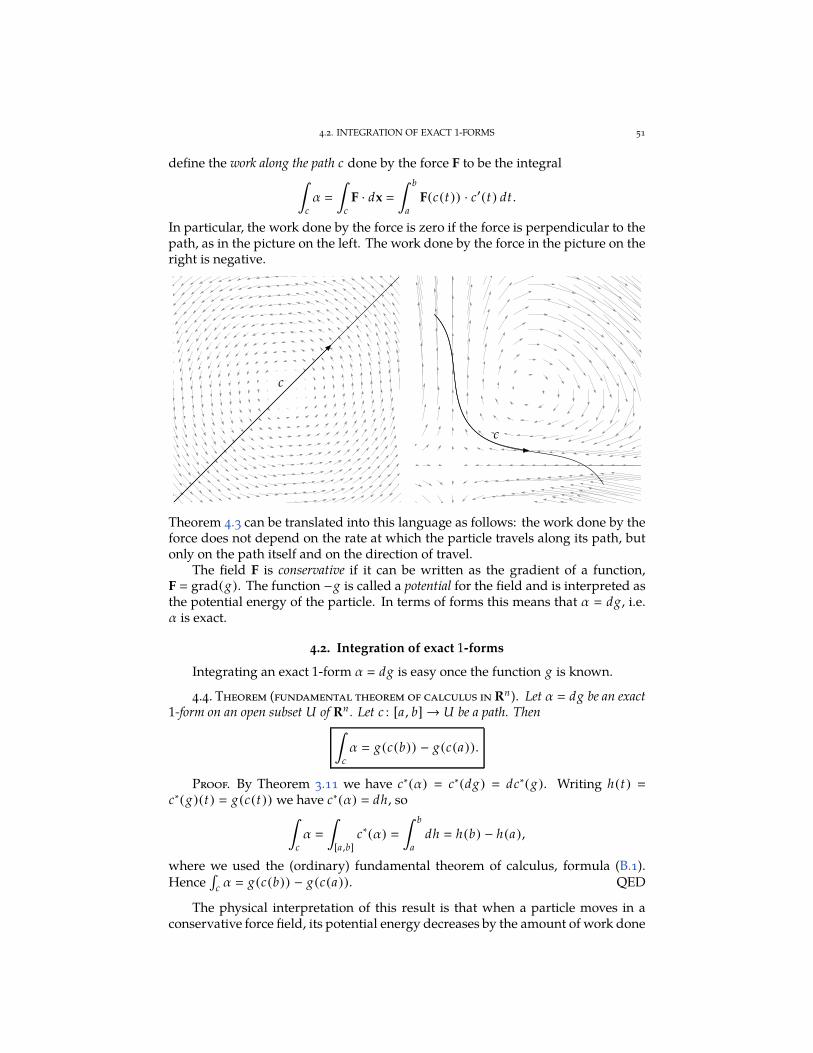
4.2. INTEGRATION OF EXACT 1-FORMS 51
define the work along the path c done by the force F to be the integral∫c
α
∫c
F · dx
∫ b
a
F(c(t)) · c′(t) dt .
In particular, the work done by the force is zero if the force is perpendicular to thepath, as in the picture on the left. The work done by the force in the picture on theright is negative.
c
c
Theorem 4.3 can be translated into this language as follows: the work done by theforce does not depend on the rate at which the particle travels along its path, butonly on the path itself and on the direction of travel.
The field F is conservative if it can be written as the gradient of a function,F grad(g). The function −g is called a potential for the field and is interpreted asthe potential energy of the particle. In terms of forms this means that α dg, i.e.α is exact.
4.2. Integration of exact 1-forms
Integrating an exact 1-form α dg is easy once the function g is known.
4.4. Theorem (fundamental theorem of calculus in Rn). Let α dg be an exact1-form on an open subset U of Rn . Let c : [a, b]→ U be a path. Then
∫c
α g(c(b)) − g(c(a)).
Proof. By Theorem 3.11 we have c∗(α) c∗(dg) dc∗(g). Writing h(t)
c∗(g)(t) g(c(t)) we have c∗(α) dh, so∫c
α
∫[a ,b]
c∗(α)
∫ b
a
dh h(b) − h(a),
where we used the (ordinary) fundamental theorem of calculus, formula (B.1).Hence
∫c α g(c(b)) − g(c(a)). QED
The physical interpretation of this result is that when a particle moves in aconservative force field, its potential energy decreases by the amount of work done
52 4. INTEGRATION OF 1-FORMS
by the field. This clarifies what it means for a field to be conservative: it meansthat the work done is entirely converted into mechanical energy and that none isdissipated by friction into heat, radiation, etc. Thus the fundamental theorem ofcalculus “explains” the law of conservation of energy.
Theorem 4.4 also gives us a necessary criterion for a 1-form on U to be exact.A path c : [a, b]→ U is called closed if c(a) c(b).
4.5. Corollary. Let α be an exact 1-form defined on an open subset U of Rn . Then∫c α 0 for every closed path c in U .
Proof. Let c : [a, b]→ U be a closed path and let g be a smooth function on Usatisfying dg α. Then
∫c α g(c(b)) − g(c(a)) 0 by Theorem 4.4. QED
This corollary can be used to detect closed 1-forms that are not exact.
4.6. Example. The angle form α0 ∈ Ω1(R2 \ 0) of Example 2.10 is closed, butnot exact. Indeed, its integral around the circle is 2π , 0, so by Corollary 4.5 α0
is not exact. Note the contrast with closed 1-forms on Rn , which are always exact!(See Exercise 2.8.)
The main content of the next theorem is that the necessary criterion of Corollary4.5 is in fact sufficient for a 1-form to be exact.
4.7. Theorem. Let α be a 1-form on a connected open subset U of Rn . Then thefollowing statements are equivalent.
(i) α is exact.(ii)
∫c α 0 for all closed paths c.
(iii)∫
c α depends only on the endpoints of c for every path c in U .
Proof. (i) ⇒ (ii): this is Corollary 4.5.(ii) ⇒ (iii): assume
∫c α 0 for all closed paths c. Let
c1 : [a1 , b1]→ U and c2 : [a2 , b2]→ U
be two paths with the same endpoints, i.e. c1(a1) c2(a2) and c1(b1) c2(b2). Weneed to show that
∫c1α
∫c2α. After reparametrizing c1 and c2 we may assume
that a1 a2 0 and b1 b2 1. Define a new path c by
c(t)
c1(t) for 0 ≤ t ≤ 1,
c2(2 − t) for 1 ≤ t ≤ 2.
(First traverse c1, then traverse c2 backwards.) Then c is closed, so∫
c α 0. ButTheorem 4.3 implies
∫c α
∫c1α −
∫c2α, so
∫c1α
∫c2α.
(iii) ⇒ (i): assume that, for all c,∫
c α depends only on the endpoints of c.We must define a function g such that α dg. Fix a point x0 in U . For each pointx in U choose a path cx : [0, 1]→ U which joins x0 to x. Define
g(x)
∫cx
α.
We assert that dg is well-defined and equal to α. Write α
∑ni1 fi dxi . We must
show that ∂g/∂xi fi . From the definition of partial differentiation,
∂g
∂xi(x) lim
h→0
g(x + hei) − g(x)
h lim
h→0
1
h
(∫cx+hei
α −∫
cx
α)
.
4.2. INTEGRATION OF EXACT 1-FORMS 53
Now consider a path c composed of two pieces: for −1 ≤ t ≤ 0 travel from x0 to xalong the path cx and then for 0 ≤ t ≤ 1 travel from x to x + hei along the straightline given by l(t) x + thei . Then c has the same endpoints as cx+hei
. Therefore∫cx+hei
α
∫c α, and hence
∂g
∂xi(x) lim
h→0
1
h
(∫c
α −∫
cx
α)
limh→0
1
h
(∫cx
α +
∫l
α −∫
cx
α)
limh→0
1
h
∫l
α limh→0
1
h
∫[0,1]
l∗(α). (4.2)
Let δi , j be the Kronecker delta, which is defined by δi ,i 1 and δi , j 0 if i , j. Thenwe can write l j (t) x j + δi , j th, and hence l′
j(t) δi , j h. This shows that
l∗(α)
n∑
j1
f j (x + thei )dl j
n∑
j1
f j (x + thei )l′j (t) dt
n∑
j1
f j (x + thei )δi , j h dt h fi (x + thei ) dt . (4.3)
Taking equations (4.2) and (4.3) together we find
∂g
∂xi(x) lim
h→0
1
h
∫ 1
0
h fi (x + thei ) dt limh→0
∫ 1
0
fi (x + thei ) dt
∫ 1
0
limh→0
fi (x + thei ) dt
∫ 1
0
fi (x) dt fi (x).
This formula shows that g is smooth and that dg α. This proves that (iii) ⇒(i), and at the same time it proves that the function g(x)
∫cxα is an antiderivative
of α. QED
Notice that the proof of the theorem tells us how to find an antiderivative ofan exact 1-form α, namely by integrating α along an arbitrary path running froma base point x0 to a variable point x. This useful fact deserves to be recordedseparately.
4.8. Theorem. Let α be an exact 1-form defined on a connected open subset U of Rn .Choose a base point x0 in U and for each x in U choose a path cx joining x0 to x. Then thefunction g(x)
∫cxα is smooth and satisfies dg α.
4.9. Example. Let α
∑ni1 fi dxi be a closed 1-form defined on all of Rn . Then
we know that α is exact. One method for finding an antiderivative is explainedin Exercise 2.8. Theorem 4.8 suggests a quicker way: let us choose the origin 0to be the base point of Rn and for each x let cx : [0, 1] → Rn be the straight path
cx(t) tx. Then g(x) ∫
cxα
∫ 1
0 c∗x(α) is an antiderivative of α. Since
c∗x(α)
n∑
i1
fi (tx) d(txi )
n∑
i1
xi fi (tx) dt
we arrive at
g(x)
n∑
i1
xi
∫ 1
0
fi (tx) dt .
54 4. INTEGRATION OF 1-FORMS
(In Exercise 4.3 you will be asked to verify directly that dg α.) For instance, letα y dx + (z cos yz + x) dy + y cos yz dz be the closed 1-form of Example 2.9. Then
g(x) x
∫ 1
0
t y dt + y
∫ 1
0
(tz cos t2 yz + tx) dt + z
∫ 1
0
t y cos t2 yz dt
2x y
∫ 1
0
t dt + 2yz
∫ 1
0
t cos t2 yz dt
x y + sin yz.
See Exercises 4.4–4.6 for further applications of this theorem.
4.3. Angle functions and the winding number
In this section we will have a closer look at the angle form and see that it carriesinteresting information of a topological nature.
Let x (x , y) be a nonzero vector in the plane and let θ(x) be the angle betweenthe positive x-axis and x. Elementary trigonometry tells us that
cos θ(x) x
√
x2 + y2, sin θ(x)
y√
x2 + y2. (4.4)
These equations determine θ(x) up to an integer multiple of 2π, and we will callany particular solution a choice of angle for x.
Now let U be an open subset of the punctured plane R2 \ 0. Is it possible tomake a choice of angle θ(x) for each x in U which varies smoothly with x? ForU R2 \ 0 this would appear to be impossible: the usual choice of angle in thepunctured plane (0 ≤ θ(x) < 2π) has a discontinuity along the positive x-axis,and there seems to be no way to get rid of this discontinuity by making a clevererchoice of angle. But it may be possible if U is a smaller open subset, such as thecomplement of the positive x-axis in R2 \ 0. Let us define an angle function on Uto be a smooth function θ : U → R with the property that θ(x) has property (4.4)for all x ∈ U . Our next result states that an angle function on U exists if and onlyif α0 is exact on U , where α0 is the angle form
α0
−y dx + x dy
x2 + y2
introduced in Example 2.10.
4.10. Theorem. Let U be a connected open subset of R2 \ 0.(i) Let θ : U → R be an angle function. Then dθ α0.
(ii) Assume that α0 is exact on U . Then there exists an angle function θ on U , whichcan be found as follows: choose a base point x0 in U , choose an angle θ0 for x0,and for each x ∈ U choose a path cx in U from x0 to x. Then θ(x) θ0 +
∫cxα0.
Proof. (i) Define functions ξ and η on the punctured plane by
ξ(x , y) x
√
x2 + y2, η(x , y)
y√
x2 + y2. (4.5)
Observe that(
ξ(x)
η(x)
)
x
‖x‖ , (4.6)
4.3. ANGLE FUNCTIONS AND THE WINDING NUMBER 55
the unit vector pointing in the direction of x (x , y). In particular
ξ(x)2 + η(x)2 1. (4.7)
We will use the result
α0 −η dξ + ξ dη (4.8)
of Exercise 2.4. If θ is an angle function on U , then ξ(x) cos θ(x) and η(x)
sin θ(x) for all x in U . Substituting this into (4.8) gives
α0 − sin θ d cos θ + cos θ d sin θ sin2 θ dθ + cos2 θ dθ dθ.
(ii) Now assume that α0 is exact on U . It follows from Theorem 4.8 that thefunction defined by θ(x) θ0 +
∫cxα0 is smooth and satisfies
dθ α0 . (4.9)
To prove that θ is an angle function on U it is enough to show that the differencevector
(
cos θ(x)
sin θ(x)
)
−(
ξ(x)
η(x)
)
has length 0 for all x. The length squared of the difference vector is equal to
(cos θ − ξ)2 + (sin θ − η)2 cos2 θ + sin2 θ − 2(ξ cos θ + η sin θ) + ξ2 + η2
2 − 2(ξ cos θ + η sin θ),
where we used (4.7). Hence we need to show that the function
u(x) ξ(x) cos θ(x) + η(x) sin θ(x)
is a constant equal to 1. For x x0 we have
u(x0) ξ(x0) cos θ0 + η(x0) sin θ0 cos2 θ0 + sin2 θ0 1,
because by assumption θ0 is a choice of angle for x0. Furthermore, the exteriorderivative of u is
du cos θ dξ − ξ sin θ dθ + sin θ dη + η cos θ dθ
cos θ dξ + sin θ dη + (−ξ sin θ + η cos θ)α0 by (4.9)
cos θ dξ + sin θ dη + (−ξ sin θ + η cos θ)(−η dξ + ξ dη) by (4.8)
(
(1 − η2) cos θ + ξη sin θ)
dξ +(
ξη cos θ + (1 − ξ2) sin θ)
dη)
(ξ cos θ + η sin θ)ξ dξ + (ξ cos θ + η sin θ))η dη by (4.7)
1
2(ξ cos θ + η sin θ) d(ξ2 + η2)
0 by (4.7).
Hence, by Lemma 3.12, u is a constant function, so u(x) 1 for all x in U . QED
4.11. Example. There exists no angle function on the punctured plane, becauseα0 is not exact on R2 \ 0 (as was shown in Example 4.6).
56 4. INTEGRATION OF 1-FORMS
Angle functions along a path. Now let us modify the angle problem by con-sidering a path c : [a, b]→ R2 \ 0 in the punctured plane and wondering whetherwe can make a choice of angle for c(t) which depends smoothly on t ∈ [a, b]. Wedefine an angle function along c to be a smooth function ϑ : [a, b] → R with theproperty that
cos ϑ(t) ξ(c(t)), sin ϑ(t) η(c(t))
for all t ∈ [a, b]. The following example shows the difference between this notionand that of an angle function on an open subset.
4.12. Example. Define c : [a, b]→ R2 \ 0 by c(t) (cos t , sin t). This is a pathtravelling along the unit circle at constant angular velocity 1 from time a to time b.The function ϑ(t) t is an angle function along c. The differenceϑ(b)−ϑ(a) b−ais the total angle swept out by the path.
In fact an angle function exists along every path in the punctured plane.
4.13. Theorem. Let c : [a, b]→ R2 \ 0 be a path. Choose an angle ϑa for c(a) andfor a ≤ t ≤ b define
ϑ(t) ϑa +
∫ t
a
c∗(α0).
The ϑ is an angle function along c.
Proof. This proof is nearly the same as that of Theorem 4.10, so we will skipsome details. We will show that the difference vector
(
cos ϑ(t)
sin ϑ(t)
)
−(
ξ(c(t))
η(c(t))
)
has length 0 for all t ∈ [a, b]. The square of the length is equal to
(cos ϑ − f )2 + (sin ϑ − g)2 cos2 ϑ + sin2 ϑ − 2( f cos ϑ + g sin ϑ) + f 2 + g2
2 − 2u,
where we introduced the abbreviations
f (t) ξ(c(t)), g(t) η(c(t)), u(t) f (t) cos ϑ(t) + g(t) sin ϑ(t),
and where we used that
f 2 + g2 1. (4.10)
Therefore it is enough to show that the function u is a constant equal to 1. Nowϑ(a) ϑa , so f (a) cos ϑ(a) and g(a) sin ϑ(a) (because ϑa is a choice of anglefor c(a)), and hence u(a) cos2 ϑa + sin2 ϑa 1. So we can finish the proof byshowing that u′(t) 0 for all t. Using (4.8) we find
c∗(α0) c∗(−η dξ + ξ dη) −c∗(η) dc∗(ξ) + c∗(ξ) dc∗(η)
−g d f + f dg (−g f ′ + f g′) dt ,
and therefore, by the fundamental theorem of calculus,
ϑ′ −g f ′ + f g′. (4.11)
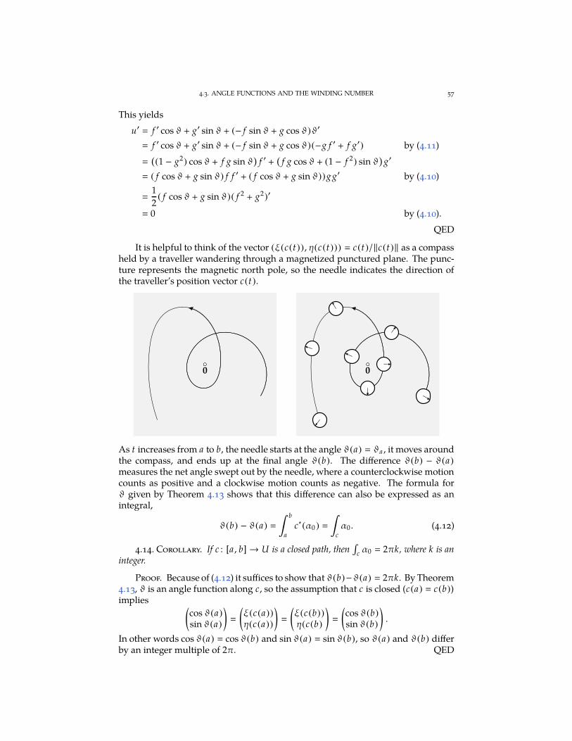
4.3. ANGLE FUNCTIONS AND THE WINDING NUMBER 57
This yields
u′ f ′ cos ϑ + g′ sin ϑ + (− f sin ϑ + g cos ϑ)ϑ′
f ′ cos ϑ + g′ sin ϑ + (− f sin ϑ + g cos ϑ)(−g f ′ + f g′) by (4.11)
(
(1 − g2) cos ϑ + f g sin ϑ)
f ′ +(
f g cos ϑ + (1 − f 2) sin ϑ)
g′
( f cos ϑ + g sin ϑ) f f ′ + ( f cos ϑ + g sin ϑ))g g′ by (4.10)
1
2( f cos ϑ + g sin ϑ)( f 2 + g2)′
0 by (4.10).
QED
It is helpful to think of the vector (ξ(c(t)), η(c(t))) c(t)/‖c(t)‖ as a compassheld by a traveller wandering through a magnetized punctured plane. The punc-ture represents the magnetic north pole, so the needle indicates the direction ofthe traveller’s position vector c(t).
0 0
As t increases from a to b, the needle starts at the angle ϑ(a) ϑa , it moves aroundthe compass, and ends up at the final angle ϑ(b). The difference ϑ(b) − ϑ(a)
measures the net angle swept out by the needle, where a counterclockwise motioncounts as positive and a clockwise motion counts as negative. The formula forϑ given by Theorem 4.13 shows that this difference can also be expressed as anintegral,
ϑ(b) − ϑ(a)
∫ b
a
c∗(α0)
∫c
α0 . (4.12)
4.14. Corollary. If c : [a, b] → U is a closed path, then∫
c α0 2πk, where k is aninteger.
Proof. Because of (4.12) it suffices to show that ϑ(b)−ϑ(a) 2πk. By Theorem4.13, ϑ is an angle function along c, so the assumption that c is closed (c(a) c(b))implies
(
cos ϑ(a)
sin ϑ(a)
)
(
ξ(c(a))
η(c(a))
)
(
ξ(c(b))
η(c(b)
)
(
cos ϑ(b)
sin ϑ(b)
)
.
In other words cos ϑ(a) cos ϑ(b) and sin ϑ(a) sin ϑ(b), so ϑ(a) and ϑ(b) differby an integer multiple of 2π. QED
58 4. INTEGRATION OF 1-FORMS
The integer k (2π)−1∫
c α0 measures how many times the path loops aroundthe origin. It is called the winding number of the closed path c about the origin, andwe will denote it by w(c, 0).
w(c, 0) winding number of c about origin
1
2π
∫c
α0 . (4.13)
4.15. Example. It follows from the calculation in Example 4.1 that the windingnumber of the circle c(t) (cos t , sin t) (0 ≤ t ≤ 2π) is equal to 1.
Exercises
4.1. Consider the path c : [0, 12π]→ R2 defined by c(t) (a cos t , b sin t), where a and
b are positive constants. Let α xy dx + x2 y dy.
(i) Sketch the path c for a 2 and b 1.(ii) Find
∫c α (for arbitrary a and b).
4.2. Restate Theorem 4.7 in terms of force fields, potentials and energy. Explain whythe result is plausible on physical grounds.
4.3. Let α
∑ni1
fi dxi be a closed 1-form defined on all of Rn .
(i) Verify that the function g(x) ∑n
i1xi
∫ 10 fi (tx) dt given in Example 4.9 satisfies
dg α.(ii) In Exercise 2.8 a different formula for the antiderivative g of α was given. Show
that that formula can be interpreted as an integral g(x)
∫cxα of α along a
suitable path cx from the origin to x.
4.4. Consider the 1-form α ‖x‖a ∑ni1
xi dxi on Rn \ 0, where a is a real constant.For every x , 0 let cx be the line segment starting at the origin and ending at x.
(i) Show that α is closed for any value of a.(ii) Determine for which values of a the function g(x)
∫cxα is well-defined and
compute it.(iii) For the values of a you found in part (ii) check that dg α.
4.5. Let α ∈ Ω1(Rn \ 0) be the 1-form of Exercise 4.4. Now let cx be the half-linepointing from x radially outward to infinity. Parametrize cx by travelling from infinityinward to x. (You can do this by using an infinite time interval (−∞, 0] in such a way thatcx(0) x.)
(i) Determine for which values of a the function g(x)
∫cxα is well-defined and
compute it.(ii) For the values of a you found in part (i) check that dg α.
(iii) Show how to recover from this computation the potential energy for Newton’sgravitational force. (See Exercise B.5.)
4.6. Let α ∈ Ω1(Rn \ 0) be as in Exercise 4.4. There is one value of a which is notcovered by Exercises 4.4 and 4.5. For this value of a find a smooth function g on Rn − 0such that dg α.
4.7. Calculate directly from the definition the winding number about the origin of the
path c : [0, 2π]→ R2 given by c(t) (cos kt , sin kt).
4.8. Let x0 be a point in R2 and c a closed path which does not pass through x0. Howwould you define the winding number w(c, x0) of c around x0? Try to formulate twodifferent definitions: a “geometric” definition and a formula in terms of an integral over cof a certain 1-form analogous to formula (4.13).
EXERCISES 59
4.9. Let c : [0, 1] → R2 \ 0 be a closed path with winding number k. Determine the
winding numbers of the following paths c : [0, 1]→ R2 \ 0 by using the formula, and thenexplain the answer by appealing to geometric intuition.
(i) c(t) c(1 − t);(ii) c(t) ρ(t)c(t), where ρ : [0, 1]→ (0,∞) is a function satisfying ρ(0) ρ(1);
(iii) c(t) ‖c(t)‖−1c(t);(iv) c(t) φ(c(t)), where φ(x, y) (y , x);
(v) c(t) φ(c(t)), where φ(x, y) 1
x2 + y2(x, −y).
4.10. For each of the following closed paths c : [0, 2π] → R2 \ 0 set up the integraldefining the winding number about the origin. Evaluate the integral if you can (but don’tgive up too soon). If not, sketch the path (the use of software is allowed) and obtain theanswer geometrically.
(i) c(t) (a cos t , b sin t), where a > 0 and b > 0;(ii) c(t) (cos t − 2, sin t);
(iii) c(t) (cos3 t , sin3 t);(iv) c(t)
(
(a cos t + b) cos t + (b − a)/2, (a cos t + b) sin t)
, where 0 < b < a.
4.11. Let b > 0 and a , 0 be constants with |a | , b. Define a path c : [0, 2π]→ R2 \ 0by
c(t)
(
(a + b) cos t + a cosa + b
at , (a + b) sin t + a sin
a + b
at)
.
(i) Sketch the path c for a ±b/3.(ii) For what values of a and b is the path closed?
(iii) Assume c is closed. Set up the integral defining the winding number of c aroundthe origin and evaluate it. If you get stuck, find the answer geometrically.
4.12. Let U be an open subset of R2 and let F F1e1 +F2e2 : U → R2 be a smooth vectorfield. The differential form
β
F1dF2 − F2dF1
F21
+ F22
is well-defined at all points x of U where F(x) , 0. Let c be a parametrized circle containedin U, traversed once in the counterclockwise direction. Assume that F(x) , 0 for all x ∈ c.The index of F relative to c is
index(F, c) 1
2π
∫cβ.
Prove the following assertions.
(i) β F∗(α0), where α0 is the angle form (−y dx + x dy)/ (
x2 + y2) ;(ii) β is closed;
(iii) index(F, c) w(F c, 0), the winding number of the path F c about the origin;(iv) index(F, c) is an integer.
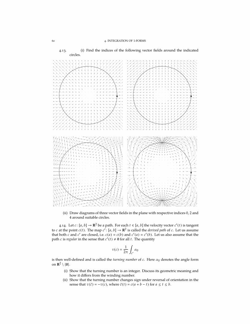
60 4. INTEGRATION OF 1-FORMS
4.13. (i) Find the indices of the following vector fields around the indicatedcircles.
(ii) Draw diagrams of three vector fields in the plane with respective indices 0, 2 and4 around suitable circles.
4.14. Let c : [a, b]→ R2 be a path. For each t ∈ [a, b] the velocity vector c′(t) is tangent
to c at the point c(t). The map c′ : [a, b] → R2 is called the derived path of c. Let us assumethat both c and c′ are closed, i.e. c(a) c(b) and c′(a) c′(b). Let us also assume that thepath c is regular in the sense that c′(t) , 0 for all t. The quantity
τ(c) 1
2π
∫c′α0
is then well-defined and is called the turning number of c. Here α0 denotes the angle form
on R2 \ 0.(i) Show that the turning number is an integer. Discuss its geometric meaning and
how it differs from the winding number.(ii) Show that the turning number changes sign under reversal of orientation in the
sense that τ(c) −τ(c), where c(t) c(a + b − t) for a ≤ t ≤ b.
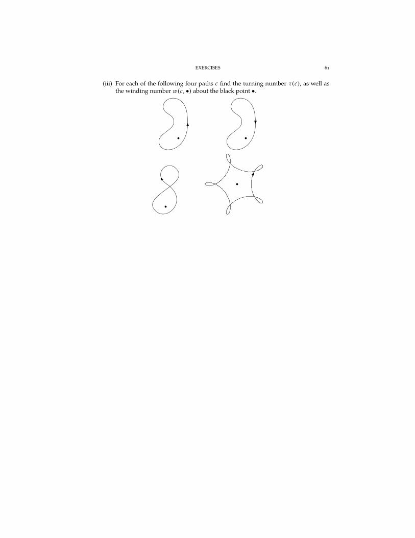
EXERCISES 61
(iii) For each of the following four paths c find the turning number τ(c), as well asthe winding number w(c, •) about the black point •.

CHAPTER 5
Integration and Stokes’ theorem
5.1. Integration of forms over chains
In this chapter we generalize the theory of Chapter 4 to higher dimensions. Inthe same way that 1-forms are integrated over parametrized curves, k-forms can beintegrated over k-dimensional parametrized regions. Let U be an open subset ofRn and let α be a k-form on U . The simplest k-dimensional analogue of an intervalis a rectangular block in Rk whose edges are parallel to the coordinate axes. This isa set of the form
R [a1 , b1] × [a2 , b2] × · · · × [ak , bk ] t ∈ Rk | ai ≤ ti ≤ bi for 1 ≤ i ≤ k ,
where ai < bi . The k-dimensional analogue of a parametrized path is a smoothmap c : R → U . Although the image c(R) may look very different from the blockR, we think of the map c as a parametrization of the subset c(R) of U : each choiceof a point t in R gives rise to a point c(t) in c(R). The pullback c∗(α) is a k-formon R and therefore looks like h(t) dt1 dt2 · · · dtk for some function h : R → R. Theintegral of α over c is defined by
∫c
α
∫R
c∗(α)
∫ bk
ak
· · ·∫ b2
a2
∫ b1
a1
h(t) dt1 dt2 · · · dtk .
(The definition of the integral makes sense if we replace the rectangular block R
by more general shapes in Rk , such as skew blocks, k-dimensional balls, cylinders,etc. In fact any compact subset of Rk will do.)
For k 1 this reproduces the definition given in Chapter 4.The case k 0 is also worth examining. A zero-dimensional “block” R in
R0 0 is just the point 0. We can therefore think of a map c : R → U as a
collection x consisting of a single point x c(0) in U . The integral of a 0-form(function) f over c is by definition the value of f at x,∫
c
f f (x).
As in the one-dimensional case, integrals of k-forms are almost completelyunaffected by a change of variables. Let
R [a1 , b1] × [a2 , b2] × · · · × [ak , bk ]
be a second rectangular block. A reparametrization is a map p : R→ R satisfying thefollowing conditions: p is bijective (i.e. one-to-one and onto) and the k × k-matrixDp(s) is invertible for all s ∈ R. Then det(Dp(s)) , 0 for all s ∈ R, so eitherdet(Dp(s)) > 0 for all s or det(Dp(s)) < 0 for all s. In these cases we say that thereparametrizion preserves, respectively reverses the orientation of c.
63
64 5. INTEGRATION AND STOKES’ THEOREM
5.1. Theorem. Let α be a k-form on U and c : R → U a smooth map. Let p : R → Rbe a reparametrization. Then
∫cpα
∫c α if p preserves the orientation,
−∫
c α if p reverses the orientation.
Proof. Almost verbatim the same proof as for k 1 (Theorem 4.3). It followsfrom the definition of the integral and from the naturality of pullbacks, Proposition3.10(iii), that ∫
cpα
∫R
(c p)∗(α)
∫R
p∗(c∗(α)).
Now let us write c∗(α) h dt1 dt2 · · · dtk and t p(s). Then
p∗(c∗(α)) p∗(h dt1 dt2 · · · dtk ) p∗(h) det(Dp) ds1 ds2 · · · dsk
by Theorem 3.14, so∫cpα
∫R
h(p(s)) det(Dp(s)) ds1 ds2 · · · dsk .
On the other hand,∫
c α
∫R h(t) dt1 dt2 · · · dtk, so by the substitution formula,
Theorem B.9, we have∫
cp α ±∫
c α, where the + occurs if det(Dp) > 0 and the −if det(Dp) < 0. QED
5.2. Example. The unit interval is the interval [0, 1] in the real line. Any pathc : [a, b] → U can be reparametrized to a path c p : [0, 1] → U by means of thereparametrization p(s) (b−a)s+a. Similarly, the unit cube in Rk is the rectangularblock
[0, 1]k t ∈ Rk | ti ∈ [0, 1] for 1 ≤ i ≤ k .
Let R be any other block, given by ai ≤ ti ≤ bi . Define p : [0, 1]k → R by p(s)
As + a, where
A
*....,
b1 − a1 0 . . . 00 b2 − a2 . . . 0...
.... . .
...0 0 . . . bk − ak
+////-
and a
*....,
a1
a2
...ak
+////-.
(“Squeeze the unit cube until it has the same edgelengths as R and then translateit to the same position as R.”) Then p is one-to-one and onto and Dp(s) A,so det(Dp(s)) det(A) vol(R) > 0 for all s, so p is an orientation-preservingreparametrization. Hence
∫cp α
∫c α for any k-form α on U .
5.3. Remark. A useful fact you learned in calculus is that one may interchangethe order of integration in a multiple integral, as in the formula
∫ b2
a2
∫ b1
a1
f (t1 , t2) dt1 dt2
∫ b1
a1
∫ b2
a2
f (t1 , t2) dt2 dt1. (5.1)
(This follows for instance from the substitution formula, Theorem B.9.) On the otherhand, we have also learned that f (t1 , t2) dt2 dt1 − f (t1, t2) dt1 dt2. How can this besquared with formula (5.1)? The explanation is as follows. Let α f (t1 , t2) dt1 dt2.Then the left-hand side of formula (5.1) is the integral of α over c : [a1 , b1]×[a2, b2]→
5.1. INTEGRATION OF FORMS OVER CHAINS 65
R2, the parametrization of the rectangle given by c(t1 , t2) (t1 , t2). The right-handside is the integral of −α not over c, but over c p, where
p : [a2 , b2] × [a1, b1]→ [a1 , b1] × [a2 , b2]
is the reparametrization p(s1 , s2) (s2 , s1). Since p reverses the orientation, Theo-rem 5.1 says that
∫cp α −
∫c α; in other words
∫c α
∫cp (−α), which is exactly
formula (5.1). Analogously we have
∫[0,1]k
f (t1 , t2, . . . , tk) dt1 dt2 · · · dtk
∫[0,1]k
f (t1 , t2, . . . , tk ) dti dt1 dt2 · · · dt i · · · dtk
for any i.
We see from Example 5.2 that an integral over any rectangular block can bewritten as an integral over the unit cube. For this reason, from now on we shallusually take R to be the unit cube. A smooth map c : [0, 1]k → U is called a k-cubein U (or sometimes a singular k-cube, the word singular meaning that the map c isnot assumed to be one-to-one, so that the image can have self-intersections.)
It is often necessary to integrate over regions that are made up of several pieces.A k-chain in U is a formal linear combination of k-cubes,
c a1c1 + a2c2 + · · · + ap cp ,
where a1, a2 , . . . , ap are real coefficients and c1, c2 , . . . , cp are k-cubes. For anyk-form α we then define
∫c
α
p∑
q1
aq
∫cq
α.
(In the language of linear algebra, the k-chains form a vector space with a basisconsisting of the k-cubes. Integration, which is a priori only defined on cubes, isextended to chains in such a way as to be linear.)
Recall that a 0-cube is nothing but a singleton x consisting of a single pointx in U . Thus a 0-chain is a formal linear combination of points, c
∑p
q1aq xq .
A good way to think of a 0-chain c is as a collection of p point charges, with anelectric charge aq placed at the point xq . (You must carefully distinguish betweenthe formal linear combination
∑p
q1aq xq, which represents a distribution of point
charges, and the linear combination of vectors∑p
q1aqxq, which represents a vector
in Rn .) The integral of a function f over the 0-chain is by definition
∫c
f
p∑
q1
aq
∫xq
f
p∑
q1
aq f (xq ).
Likewise, a k-chain∑p
q1aqcq can be pictured as a charge distribution, with an
electric charge aq spread along the k-dimensional “patch” cq .
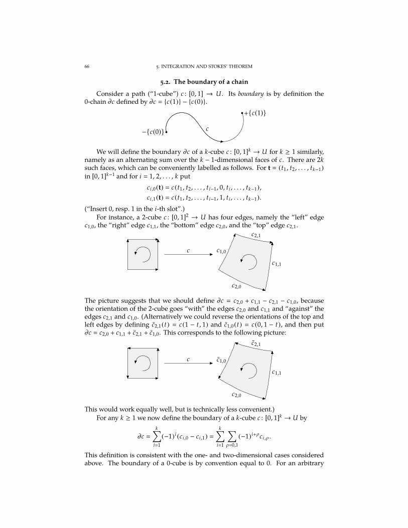
66 5. INTEGRATION AND STOKES’ THEOREM
5.2. The boundary of a chain
Consider a path (“1-cube”) c : [0, 1] → U . Its boundary is by definition the0-chain ∂c defined by ∂c c(1) − c(0).
−c(0)
+c(1)
c
We will define the boundary ∂c of a k-cube c : [0, 1]k → U for k ≥ 1 similarly,namely as an alternating sum over the k − 1-dimensional faces of c. There are 2ksuch faces, which can be conveniently labelled as follows. For t (t1 , t2, . . . , tk−1)
in [0, 1]k−1 and for i 1, 2, . . . , k put
ci ,0(t) c(t1 , t2, . . . , ti−1, 0, ti , . . . , tk−1),
ci ,1(t) c(t1 , t2, . . . , ti−1, 1, ti , . . . , tk−1).
(“Insert 0, resp. 1 in the i-th slot”.)For instance, a 2-cube c : [0, 1]2 → U has four edges, namely the “left” edge
c1,0, the “right” edge c1,1, the “bottom” edge c2,0, and the “top” edge c2,1.
c
c2,0
c1,1
c2,1
c1,0
The picture suggests that we should define ∂c c2,0 + c1,1 − c2,1 − c1,0, becausethe orientation of the 2-cube goes “with” the edges c2,0 and c1,1 and “against” theedges c2,1 and c1,0. (Alternatively we could reverse the orientations of the top andleft edges by defining c2,1(t) c(1 − t , 1) and c1,0(t) c(0, 1 − t), and then put∂c c2,0 + c1,1 + c2,1 + c1,0. This corresponds to the following picture:
c
c2,0
c1,1
c2,1
c1,0
This would work equally well, but is technically less convenient.)For any k ≥ 1 we now define the boundary of a k-cube c : [0, 1]k → U by
∂c
k∑
i1
(−1)i (ci ,0 − ci ,1)
k∑
i1
∑
ρ0,1
(−1)i+ρci ,ρ .
This definition is consistent with the one- and two-dimensional cases consideredabove. The boundary of a 0-cube is by convention equal to 0. For an arbitrary
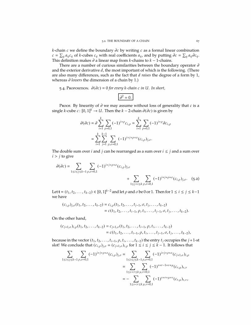
5.2. THE BOUNDARY OF A CHAIN 67
k-chain c we define the boundary ∂c by writing c as a formal linear combinationc
∑
q aq cq of k-cubes cq with real coefficients aq , and by putting ∂c
∑
q aq∂cq .This definition makes ∂ a linear map from k-chains to k − 1-chains.
There are a number of curious similarities between the boundary operator ∂and the exterior derivative d, the most important of which is the following. (Thereare also many differences, such as the fact that d raises the degree of a form by 1,whereas ∂ lowers the dimension of a chain by 1.)
5.4. Proposition. ∂(∂c) 0 for every k-chain c in U . In short,
∂2 0.
Proof. By linearity of ∂ we may assume without loss of generality that c is asingle k-cube c : [0, 1]k → U . Then the k − 2-chain ∂(∂c) is given by
∂(∂c) ∂k∑
i1
∑
ρ0,1
(−1)i+ρci ,ρ
k∑
i1
∑
ρ0,1
(−1)i+ρ∂ci ,ρ
k∑
i1
k−1∑
j1
∑
ρ,σ0,1
(−1)i+ j+ρ+σ(ci ,ρ) j,σ .
The double sum over i and j can be rearranged as a sum over i ≤ j and a sum overi > j to give
∂(∂c) ∑
1≤i≤ j≤k−1
∑
ρ,σ0,1
(−1)i+ j+ρ+σ(ci ,ρ ) j,σ
+∑
1≤ j<i≤k
∑
ρ,σ0,1
(−1)i+ j+ρ+σ(ci ,ρ) j,σ . (5.2)
Let t (t1, t2, . . . , tk−2) ∈ [0, 1]k−2 and let ρ and σ be 0 or 1. Then for 1 ≤ i ≤ j ≤ k−1we have
(ci ,ρ) j,σ(t1 , t2, . . . , tk−2) ci ,ρ (t1, t2, . . . , t j−1, σ, t j , . . . , tk−2)
c(t1 , t2, . . . , ti−1, ρ, ti , . . . , t j−1, σ, t j , . . . , tk−2).
On the other hand,
(c j+1,σ )i ,ρ(t1, t2, . . . , tk−2) c j+1,σ (t1 , t2, . . . , ti−1, ρ, ti , . . . , tk−2)
c(t1 , t2, . . . , ti−1, ρ, ti , . . . , t j−1, σ, t j , . . . , tk−2),
because in the vector (t1, t2, . . . , ti−1, ρ, ti , . . . , tk−2) the entry t j occupies the j +1-stslot! We conclude that (ci ,ρ) j,σ (c j+1,σ)i ,ρ for 1 ≤ i ≤ j ≤ k − 1. It follows that
∑
1≤i≤ j≤k−1
∑
ρ,σ0,1
(−1)i+ j+ρ+σ(ci ,ρ ) j,σ
∑
1≤i≤ j≤k−1
∑
ρ,σ0,1
(−1)i+ j+ρ+σ(c j+1,σ )i ,ρ
∑
1≤s<r≤k
∑
µ,ν0,1
(−1)s+r−1+ν+µ(cr,µ)s ,ν
−∑
1≤s<r≤k
∑
µ,ν0,1
(−1)s+r+µ+ν(cr,µ)s ,ν ,
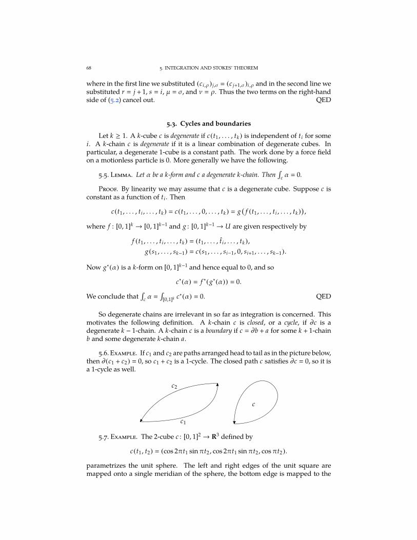
68 5. INTEGRATION AND STOKES’ THEOREM
where in the first line we substituted (ci ,ρ) j,σ (c j+1,σ )i ,ρ and in the second line wesubstituted r j + 1, s i, µ σ, and ν ρ. Thus the two terms on the right-handside of (5.2) cancel out. QED
5.3. Cycles and boundaries
Let k ≥ 1. A k-cube c is degenerate if c(t1 , . . . , tk ) is independent of ti for somei. A k-chain c is degenerate if it is a linear combination of degenerate cubes. Inparticular, a degenerate 1-cube is a constant path. The work done by a force fieldon a motionless particle is 0. More generally we have the following.
5.5. Lemma. Let α be a k-form and c a degenerate k-chain. Then∫
c α 0.
Proof. By linearity we may assume that c is a degenerate cube. Suppose c isconstant as a function of ti. Then
c(t1 , . . . , ti , . . . , tk) c(t1 , . . . , 0, . . . , tk ) g(
f (t1 , . . . , ti , . . . , tk ))
,
where f : [0, 1]k → [0, 1]k−1 and g : [0, 1]k−1→ U are given respectively by
f (t1 , . . . , ti , . . . , tk) (t1 , . . . , ti , . . . , tk ),
g(s1 , . . . , sk−1) c(s1 , . . . , si−1, 0, si+1, . . . , sk−1).
Now g∗(α) is a k-form on [0, 1]k−1 and hence equal to 0, and so
c∗(α) f ∗(g∗(α)) 0.
We conclude that∫
c α
∫[0,1]k c∗(α) 0. QED
So degenerate chains are irrelevant in so far as integration is concerned. Thismotivates the following definition. A k-chain c is closed, or a cycle, if ∂c is adegenerate k − 1-chain. A k-chain c is a boundary if c ∂b + a for some k + 1-chainb and some degenerate k-chain a.
5.6. Example. If c1 and c2 are paths arranged head to tail as in the picture below,then ∂(c1 + c2) 0, so c1 + c2 is a 1-cycle. The closed path c satisfies ∂c 0, so it isa 1-cycle as well.
c1
c2
c
5.7. Example. The 2-cube c : [0, 1]2 → R3 defined by
c(t1 , t2) (cos 2πt1 sinπt2 , cos 2πt1 sin πt2 , cosπt2).
parametrizes the unit sphere. The left and right edges of the unit square aremapped onto a single meridian of the sphere, the bottom edge is mapped to the
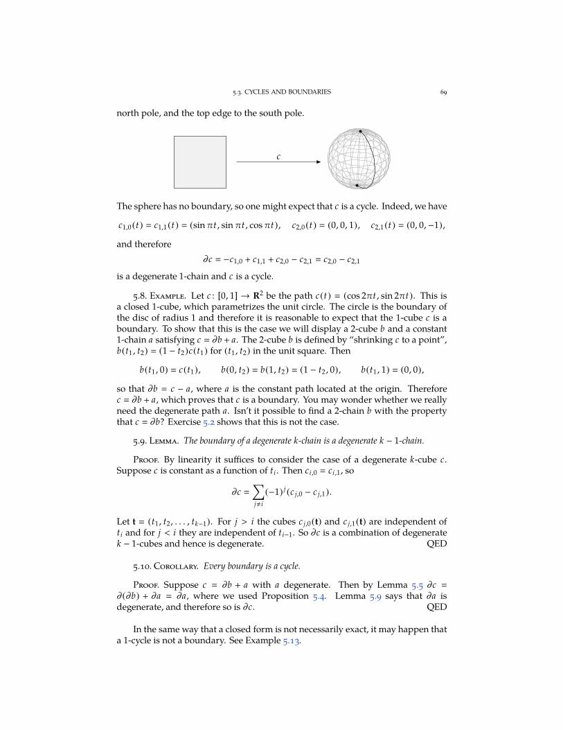
5.3. CYCLES AND BOUNDARIES 69
north pole, and the top edge to the south pole.
c
The sphere has no boundary, so one might expect that c is a cycle. Indeed, we have
c1,0(t) c1,1(t) (sin πt , sin πt , cos πt), c2,0(t) (0, 0, 1), c2,1(t) (0, 0,−1),
and therefore
∂c −c1,0 + c1,1 + c2,0 − c2,1 c2,0 − c2,1
is a degenerate 1-chain and c is a cycle.
5.8. Example. Let c : [0, 1] → R2 be the path c(t) (cos 2πt , sin 2πt). This isa closed 1-cube, which parametrizes the unit circle. The circle is the boundary ofthe disc of radius 1 and therefore it is reasonable to expect that the 1-cube c is aboundary. To show that this is the case we will display a 2-cube b and a constant1-chain a satisfying c ∂b + a. The 2-cube b is defined by “shrinking c to a point”,b(t1 , t2) (1 − t2)c(t1) for (t1, t2) in the unit square. Then
b(t1 , 0) c(t1), b(0, t2) b(1, t2) (1 − t2 , 0), b(t1 , 1) (0, 0),
so that ∂b c − a, where a is the constant path located at the origin. Thereforec ∂b + a, which proves that c is a boundary. You may wonder whether we reallyneed the degenerate path a. Isn’t it possible to find a 2-chain b with the propertythat c ∂b? Exercise 5.2 shows that this is not the case.
5.9. Lemma. The boundary of a degenerate k-chain is a degenerate k − 1-chain.
Proof. By linearity it suffices to consider the case of a degenerate k-cube c.Suppose c is constant as a function of ti. Then ci ,0 ci ,1, so
∂c
∑
j,i
(−1) j (c j,0 − c j,1).
Let t (t1 , t2, . . . , tk−1). For j > i the cubes c j,0(t) and c j,1(t) are independent ofti and for j < i they are independent of ti−1. So ∂c is a combination of degeneratek − 1-cubes and hence is degenerate. QED
5.10. Corollary. Every boundary is a cycle.
Proof. Suppose c ∂b + a with a degenerate. Then by Lemma 5.5 ∂c
∂(∂b) + ∂a ∂a, where we used Proposition 5.4. Lemma 5.9 says that ∂a isdegenerate, and therefore so is ∂c. QED
In the same way that a closed form is not necessarily exact, it may happen thata 1-cycle is not a boundary. See Example 5.13.
70 5. INTEGRATION AND STOKES’ THEOREM
5.4. Stokes’ theorem
In the language of chains and boundaries we can rewrite the fundamentaltheorem of calculus, Theorem 4.4, as follows:∫
c
dg g(c(1)) − g(c(0))
∫c(1)
g −∫c(0)
g
∫c(1)−c(0)
g
∫∂c
g ,
i.e.∫
c dg
∫∂c g. This is the form in which the fundamental theorem of calculus
generalizes to higher dimensions. This generalization is perhaps the neatest rela-tionship between the exterior derivative and the boundary operator. It containsas special cases the classical integration formulas of vector calculus (Green, Gaussand Stokes) and for that reason has Stokes’ name attached to it, although it wouldperhaps be better to call it the “fundamental theorem of multivariable calculus”.
5.11. Theorem (Stokes’ theorem). Let α be a k − 1-form on an open subset U of Rn
and let c be a k-chain in U . Then∫
c
dα
∫∂c
α.
Proof. Let us assume, as we may, that c : [0, 1]k → U is a single k-cube. By thedefinition of the integral and by Theorem 3.11 we have∫
c
dα
∫[0,1]k
c∗(dα)
∫[0,1]k
dc∗(α).
Since c∗(α) is a k − 1-form on [0, 1]k, it can be written as
c∗(α)
k∑
i1
gi dt1 dt2 · · · dt i · · · dtk
for certain functions g1, g2 , . . . , gk defined on [0, 1]k. Therefore
∫c
dα
k∑
i1
∫[0,1]k
d(
gi dt1 dt2 · · · dt i · · · dtk)
k∑
i1
(−1)i+1
∫[0,1]k
∂gi
∂tidt1 dt2 · · · dtk .
Changing the order of integration (see Remark 5.3) and subsequently applying thefundamental theorem of calculus in one variable, formula (B.1), gives
∫[0,1]k
∂gi
∂tidt1 dt2 · · · dtk
∫[0,1]k
∂gi
∂tidti dt1 dt2 · · · dt i · · · dtk
∫[0,1]k−1
(
gi (t1, . . . , ti−1, 1, ti+1, . . . , tk)
− gi (t1 , . . . , ti−1, 0, ti+1, . . . , tk ))
dt1 dt2 · · · dt i · · · dtk .
The forms
gi (t1 , . . . , ti−1, 1, ti+1, . . . , tk ) dt1 dt2 · · · dt i · · · dtk and
gi (t1 , . . . , ti−1, 0, ti+1, . . . , tk ) dt1 dt2 · · · dt i · · · dtk
EXERCISES 71
are nothing but c∗i ,1
(α), resp. c∗i ,0
(α). Accordingly,
∫c
dα
k∑
i1
(−1)i+1
∫[0,1]k
∂gi
∂tidti dt1 dt2 · · · dt i · · · dtk
k∑
i1
(−1)i+1
∫[0,1]k−1
(
c∗i ,1(α) − c∗i ,0(α))
k∑
i1
∑
ρ0,1
(−1)i+ρ
∫[0,1]k−1
c∗i ,ρ(α)
k∑
i1
∑
ρ0,1
(−1)i+ρ
∫ci,ρ
α
∫∂c
α,
which proves the result. QED
5.12. Corollary. Let U be an open subset of Rn , let c be a k-chain in U , and let α bea k-form on U . Then
∫c α 0 if either of the following two conditions holds:
(i) c is a cycle and α is exact; or(ii) c is a boundary and α is closed.
Proof. (i) If c is a cycle, then ∂c is a degenerate k − 1-chain. If α is exact, thenα dβ for some k − 1-form β. Therefore
∫c α
∫c dβ
∫∂c β 0 by Stokes’ theorem
and by Lemma 5.5.(ii) If c is a boundary, then c ∂b+a for some k+1-chain b and some degenerate
k-chain a. If α is closed, then dα 0. Therefore∫
c α
∫∂b+a α
∫b dα +
∫a α 0 by
Stokes’ theorem and by Lemma 5.5. QED
5.13. Example. The unit circle c(t) (cos 2πt , sin 2πt) (0 ≤ t ≤ 1) is a 1-cyclein the punctured plane U R2 \ 0. Considered as a chain in R2 it is also aboundary, as we saw in Example 5.8. However, we claim that it is not a boundaryin U : it is impossible to find a 2-chain b and a degenerate 1-chain a both containedin U such that c ∂b + a. Indeed, suppose this was possible. Then
∫c α0 0 by
Corollary 5.12, where α0 is the angle form, because α0 is closed. On the other hand,by Example 4.1 we have
∫c α0 2π. This is a contradiction, so we conclude that
c is not a boundary in U . The presence of the puncture in U is responsible bothfor the existence of the non-exact closed 1-form α0 (see Example 4.6) and for thenon-bounding closed 1-chain c.
Exercises
5.1. Let U be an open subset of Rn , V an open subset of Rm and φ : U → V a smoothmap. Let c be a k-cube in U and α a k-form on V . Prove that
∫c φ∗(α)
∫φc α.
5.2. Let U be an open subset of Rn .
(i) Let b be a k + 1-chain in U. In Section 5.2 we defined the boundary of b as acertain linear combination of k-cubes, ∂b
∑
i ai ci . Prove that∑
i ai 0.(ii) Let c be a k-cube in U. Prove that there exists no k + 1-chain b in U satisfying
∂b c.
5.3. Define a 2-cube c : [0, 1]2 → R3 by c(t1 , t2)
(
t21, t1t2 , t
22
)
, and let α x1 dx2 +
x1 dx3 + x2 dx3.
72 5. INTEGRATION AND STOKES’ THEOREM
(i) Sketch the image of c.(ii) Calculate both
∫c dα and
∫∂c α and check that they are equal.
5.4. Define a 3-cube c : [0, 1]3 → R3 by c(t1 , t2 , t3) (t2t3 , t1t3 , t1t2), and let α
x1 dx2 dx3 . Calculate both∫
c dα and∫∂c α and check that they are equal.
5.5. Using polar coordinates in n dimensions (see Exercise 3.19) write the n − 1-dimen-
sional unit sphere Sn−1 in Rn as the image of an n − 1-cube c. (The domain of c will not be
the unit cube in Rn−1, but a rectangular block R. Choose R in such a way as to cover thesphere as economically as possible.) For n 2, 3, 4, calculate the boundary ∂c and showthat c is a cycle. (See also Example 5.7.)
5.6. Deduce the following classical integration formulas from the generalized versionof Stokes’ theorem. All functions, vector fields, chains etc. are smooth and are defined in anopen subset U of Rn . (Some formulas hold only for special values of n, as indicated.)
(i)
∫c
grad(g) · dx g(c(1)) − g(c(0)) for any function g and any path c.
(ii) Green’s formula:
∫c
( ∂g
∂x−∂ f
∂y
)
dx dy
∫∂c
( f dx + g dy) for any functions f , g
and any 2-chain c. (Here n 2.)
(iii) Gauss’ formula:
∫c
div(F) dx1 dx2 · · · dxn
∫∂c
F · ∗dx for any vector field F and
any n-chain c.
(iv) Stokes’ formula:
∫c
curl(F) · ∗dx
∫∂c
F · dx for any vector field F and any 2-chain
c. (Here n 3.)
In parts (iii) and (iv) we use the notations dx and ∗dx explained in Section 2.5. We shall givea geometric interpretation of the entity ∗dx in terms of volume forms later on. (See Corollary8.17.)
5.7. An Rr-valued k-form on an open subset U of Rn is a vector
α
*.....,
α1α2...αr
+/////-,
whose entries α1, α2 , . . . , αr are ordinary k-forms defined on U. The number r can be anynonnegative integer and does not have to be related to n or k. Sometimes we leave thevalue of r unspecified and speak of α as a vector-valued k-form. Examples of vector-valueddifferential forms are the Rn-valued 1-form dx and the Rn-valued n − 1-form ∗dx on Rn
introduced in Section 2.5. The integral of an Rr-valued k-form α over a k-chain c in U isdefined by
∫cα
*.....,
∫c α1∫c α2...∫
c αr
+/////-.
This integral is a vector in Rr . Prove the following extensions of Gauss’ divergence formulato vector-valued forms.
(i) The gradient version:
∫c
grad( f ) dx1 dx2 · · · dxn
∫∂c
f ∗dx for any function f
and any n-chain c. (Here r n.)
EXERCISES 73
(ii) The curl version:
∫c
curl(F) dx1 dx2 dx3 −∫∂c
F × dx for any vector field F and
any 3-chain c. (Here r n 3.)
Both formulas can be deduced from Exercise 5.6(iii) by considering each component of thevector-valued integrals separately. Gauss’ formulas look more suggestive if we employ thenabla notation of vector calculus. Writing ∇ f grad( f ), ∇ · F div(F) and ∇ × F curl(F)
we get: ∫c∇ · F dx1 dx2 · · · dxn
∫∂c
F · ∗dx
∫c∇ f dx1 dx2 · · · dxn
∫∂c
f ∗dx
∫c∇ × F dx1 dx2 dx3 −
∫∂c
F × ∗dx.
5.8. Prove the following extensions of Stokes’ formula to R3-valued forms on R3. (SeeExercise 5.7 for an explanation of vector-valued forms.)
(i) The gradient version:
∫c
grad( f ) × ∗dx −∫∂c
f dx for any function f and any
2-chain c.
(ii) The divergence version:
∫c
(
div(F) − DFT ) ∗dx
∫∂c
F × dx for any vector field F
and any 2-chain c. Here DFT denotes the transpose of the Jacobi matrix of F.
The expression(
div(F) − DFT ) ∗dx is shorthand for div(F) ∗dx − DFT ∗dx. The
first term div(F) ∗dx is the product of the function div(F) and the R3-valued form
∗dx and the second term DFT∗dx is the product of the 3 × 3-matrix DFT and the
R3-valued 2-form ∗dx.
In nabla notation Stokes’ formulas look as follows:∫c(∇ × F) · ∗dx
∫∂c
F · dx
∫c∇ f × ∗dx −
∫∂c
f dx
∫c
(∇ · F −DFT ) ∗dx
∫∂c
F × dx.

CHAPTER 6
Manifolds
6.1. The definition
Intuitively, an n-dimensional manifold in the Euclidean space RN is a subsetthat in the neighbourhood of every point “looks like” Rn up to “smooth distor-tions”. The formal definition is given below and is a bit long. It will help to considerfirst the basic example of the surface of the earth, which is a two-dimensional sphereplaced in three-dimensional space. Geographers describe the earth by means ofa world atlas, which is a collection of maps. Each map depicts a portion of theworld, such as a country or an ocean. The correspondence between points on amap and points on the earth’s surface is not entirely faithful, because charting acurved surface on a flat piece of paper inevitably distorts the distances betweenpoints. But the distortions are continuous, indeed differentiable (in most tradi-tional cartographic projections). Maps of neighbouring areas overlap near theiredges and the totality of all maps in a world atlas covers the whole world.
An arbitrary manifold is defined similarly, as an n-dimensional “world” rep-resented by an “atlas” consisting of “maps”. These maps are a special kind ofparametrizations known as embeddings.
6.1. Definition. Let U be an open subset of Rn . An embedding of U into RN isa C∞ map ψ : U → RN satisfying the following conditions:
(i) ψ is one-to-one (i.e. if ψ(t1) ψ(t2), then t1 t2);(ii) Dψ(t) is one-to-one for all t ∈ U ;
(iii) the inverse of ψ, which is a map ψ−1 : ψ(U) → U , is continuous.
The image of the embedding is the set ψ(U) ψ(t) | t ∈ U consisting of allpoints of the form ψ(t) with t ∈ U . You should think of ψ(U) as an n-dimensional“patch” in RN parametrized by the map ψ. The inverse map ψ−1 is called a chartor coordinate map. It maps each point in the patch ψ(U) to an n-tuple of numbers,which we think of as the “coordinates” of the point. Condition (i) means that todistinct values of the parameter t must correspond distinct points ψ(t) in the patchψ(U). Thus the patch ψ(U) has no self-intersections. Condition (ii) means that foreach t in U all n columns of the Jacobi matrix Dψ(t) must be independent. Thiscondition is imposed to prevent the occurrence of cusps and other singularities inthe image ψ(U). Since Dψ(t) has N rows, condition (ii) also implies that N ≥ n:the target space RN must have dimension greater than or equal to that of thesource space U , or else ψ cannot be an embedding. Condition (iii) can be restatedas follows: if ti is any sequence of points in U such that limi→∞ ψ(ti ) exists and isequal to ψ(t) for some t ∈ U , then limi→∞ ti t. This is intended to avoid situationswhere the image ψ(U) doubles back on itself “at infinity”. (See Exercise 6.4 for an
75
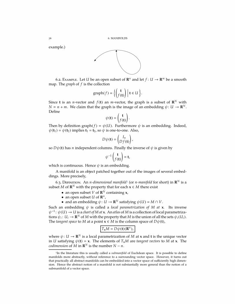
76 6. MANIFOLDS
example.)
6.2. Example. Let U be an open subset of Rn and let f : U → Rm be a smoothmap. The graph of f is the collection
graph( f )
(
tf (t)
) t ∈ U
.
Since t is an n-vector and f (t) an m-vector, the graph is a subset of RN withN n + m. We claim that the graph is the image of an embedding ψ : U → RN .Define
ψ(t)
(
tf (t)
)
.
Then by definition graph( f ) ψ(U). Furthermore ψ is an embedding. Indeed,ψ(t1) ψ(t2) implies t1 t2, so ψ is one-to-one. Also,
Dψ(t)
(
In
D f (t)
)
,
so Dψ(t) has n independent columns. Finally the inverse of ψ is given by
ψ−1
(
tf (t)
)
t,
which is continuous. Hence ψ is an embedding.
A manifold is an object patched together out of the images of several embed-dings. More precisely,
6.3. Definition. An n-dimensional manifold1 (or n-manifold for short) in RN is asubset M of RN with the property that for each x ∈ M there exist
• an open subset V of RN containing x,• an open subset U of Rn ,• and an embedding ψ : U → RN satisfying ψ(U) M ∩ V.
Such an embedding ψ is called a local parametrization of M at x. Its inverseψ−1 : ψ(U) → U is a chart of M at x. An atlas of M is a collection of local parametriza-tions ψi : Ui → RN of M with the property that M is the union of all the sets ψi (Ui).The tangent space to M at a point x ∈ M is the column space of Dψ(t),
TxM Dψ(t)(Rn ),
where ψ : U → RN is a local parametrization of M at x and t is the unique vectorin U satisfying ψ(t) x. The elements of TxM are tangent vectors to M at x. Thecodimension of M in RN is the number N − n.
1In the literature this is usually called a submanifold of Euclidean space. It is possible to definemanifolds more abstractly, without reference to a surrounding vector space. However, it turns outthat practically all abstract manifolds can be embedded into a vector space of sufficiently high dimen-sion. Hence the abstract notion of a manifold is not substantially more general than the notion of a
submanifold of a vector space.
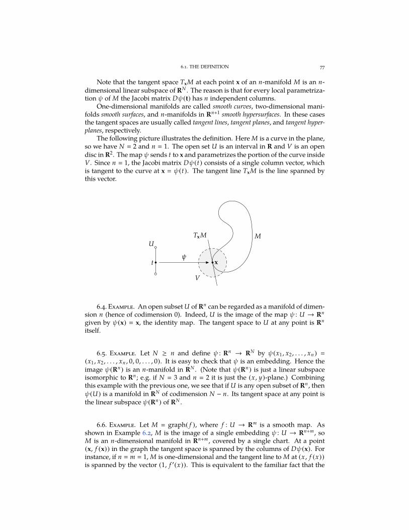
6.1. THE DEFINITION 77
Note that the tangent space TxM at each point x of an n-manifold M is an n-dimensional linear subspace of RN . The reason is that for every local parametriza-tion ψ of M the Jacobi matrix Dψ(t) has n independent columns.
One-dimensional manifolds are called smooth curves, two-dimensional mani-folds smooth surfaces, and n-manifolds in Rn+1 smooth hypersurfaces. In these casesthe tangent spaces are usually called tangent lines, tangent planes, and tangent hyper-planes, respectively.
The following picture illustrates the definition. Here M is a curve in the plane,so we have N 2 and n 1. The open set U is an interval in R and V is an opendisc in R2. The map ψ sends t to x and parametrizes the portion of the curve insideV. Since n 1, the Jacobi matrix Dψ(t) consists of a single column vector, whichis tangent to the curve at x ψ(t). The tangent line TxM is the line spanned bythis vector.
t
U
V
M
x
TxM
ψ
6.4. Example. An open subset U of Rn can be regarded as a manifold of dimen-sion n (hence of codimension 0). Indeed, U is the image of the map ψ : U → Rn
given by ψ(x) x, the identity map. The tangent space to U at any point is Rn
itself.
6.5. Example. Let N ≥ n and define ψ : Rn → RN by ψ(x1 , x2 , . . . , xn )
(x1 , x2 , . . . , xn , 0, 0, . . . , 0). It is easy to check that ψ is an embedding. Hence theimage ψ(Rn) is an n-manifold in RN . (Note that ψ(Rn ) is just a linear subspaceisomorphic to Rn ; e.g. if N 3 and n 2 it is just the (x , y)-plane.) Combiningthis example with the previous one, we see that if U is any open subset of Rn , thenψ(U) is a manifold in RN of codimension N − n. Its tangent space at any point isthe linear subspace ψ(Rn ) of RN .
6.6. Example. Let M graph( f ), where f : U → Rm is a smooth map. Asshown in Example 6.2, M is the image of a single embedding ψ : U → Rn+m, soM is an n-dimensional manifold in Rn+m , covered by a single chart. At a point(x, f (x)) in the graph the tangent space is spanned by the columns of Dψ(x). Forinstance, if n m 1, M is one-dimensional and the tangent line to M at (x , f (x))
is spanned by the vector (1, f ′(x)). This is equivalent to the familiar fact that the
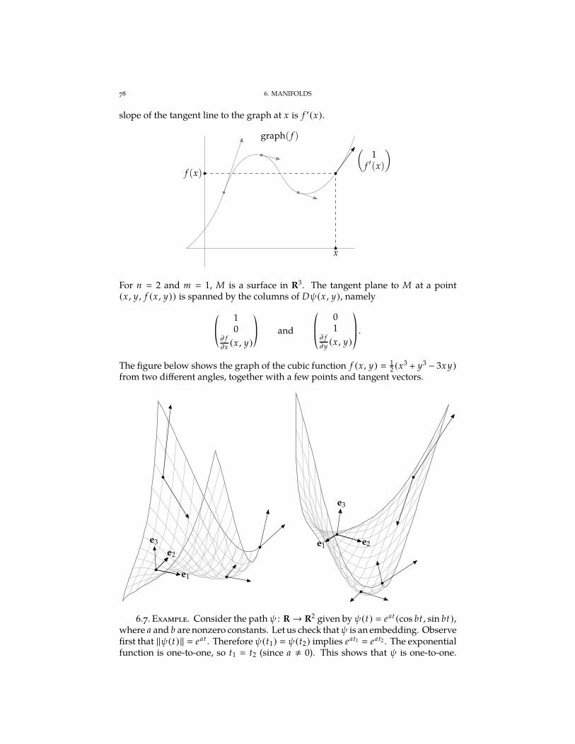
78 6. MANIFOLDS
slope of the tangent line to the graph at x is f ′(x).
x
f (x)
(
1f ′(x)
)
graph( f )
For n 2 and m 1, M is a surface in R3. The tangent plane to M at a point(x , y , f (x , y)) is spanned by the columns of Dψ(x , y), namely
*.,
10
∂ f
∂x (x , y)
+/-
and*..,
01
∂ f
∂y(x , y)
+//-.
The figure below shows the graph of the cubic function f (x , y) 12 (x3 + y3 − 3x y)
from two different angles, together with a few points and tangent vectors.
e1
e2
e3 e1 e2
e3
6.7. Example. Consider the path ψ : R→ R2 given by ψ(t) eat (cos bt , sin bt),where a and b are nonzero constants. Let us check thatψ is an embedding. Observefirst that ‖ψ(t)‖ eat . Therefore ψ(t1) ψ(t2) implies eat1
eat2 . The exponentialfunction is one-to-one, so t1 t2 (since a , 0). This shows that ψ is one-to-one.
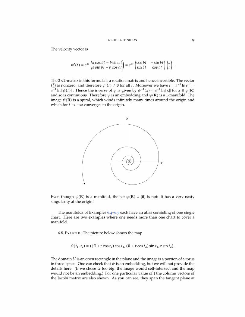
6.1. THE DEFINITION 79
The velocity vector is
ψ′(t) eat
(
a cos bt − b sin bta sin bt + b cos bt
)
eat
(
cos bt − sin btsin bt cos bt
) (
ab
)
.
The 2×2-matrix in this formula is a rotation matrix and hence invertible. The vector(a
b
)
is nonzero, and therefore ψ′(t) , 0 for all t. Moreover we have t a−1 ln eat
a−1 ln‖ψ(t)‖. Hence the inverse of ψ is given by ψ−1(x) a−1 ln‖x‖ for x ∈ ψ(R)
and so is continuous. Therefore ψ is an embedding and ψ(R) is a 1-manifold. Theimage ψ(R) is a spiral, which winds infinitely many times around the origin andwhich for t → −∞ converges to the origin.
x
y
Even though ψ(R) is a manifold, the set ψ(R) ∪ 0 is not: it has a very nastysingularity at the origin!
The manifolds of Examples 6.4–6.7 each have an atlas consisting of one singlechart. Here are two examples where one needs more than one chart to cover amanifold.
6.8. Example. The picture below shows the map
ψ(t1, t2) (
(R + r cos t2) cos t1, (R + r cos t2) sin t1, r sin t2)
.
The domain U is an open rectangle in the plane and the image is a portion of a torusin three-space. One can check that ψ is an embedding, but we will not provide thedetails here. (If we chose U too big, the image would self-intersect and the mapwould not be an embedding.) For one particular value of t the column vectors ofthe Jacobi matrix are also shown. As you can see, they span the tangent plane at
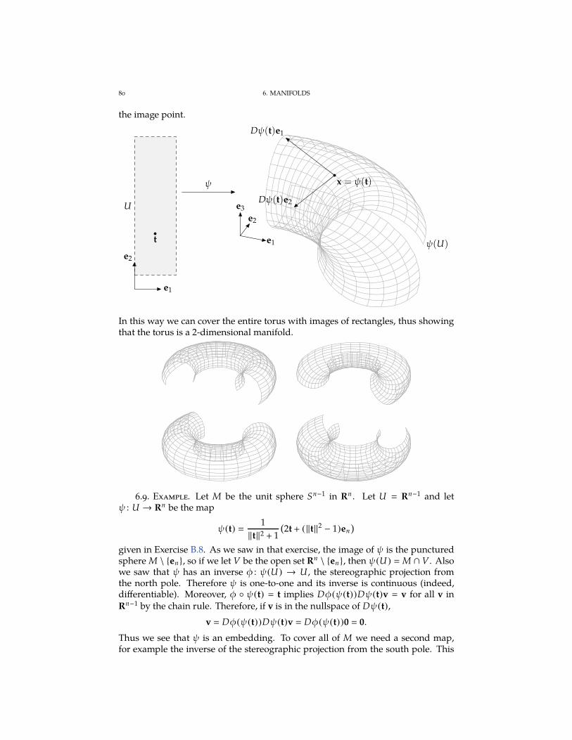
80 6. MANIFOLDS
the image point.
x = ψ(t)
Dψ(t)e1
Dψ(t)e2
ψ(U)t
U
e1
e2
e1
e2
e3
ψ
In this way we can cover the entire torus with images of rectangles, thus showingthat the torus is a 2-dimensional manifold.
6.9. Example. Let M be the unit sphere Sn−1 in Rn . Let U Rn−1 and letψ : U → Rn be the map
ψ(t) 1
‖t‖2 + 1
(
2t + (‖t‖2 − 1)en)
given in Exercise B.8. As we saw in that exercise, the image of ψ is the puncturedsphere M \ en , so if we let V be the open set Rn \ en , then ψ(U) M ∩V. Alsowe saw that ψ has an inverse φ : ψ(U) → U , the stereographic projection fromthe north pole. Therefore ψ is one-to-one and its inverse is continuous (indeed,differentiable). Moreover, φ ψ(t) t implies Dφ(ψ(t))Dψ(t)v v for all v inRn−1 by the chain rule. Therefore, if v is in the nullspace of Dψ(t),
v Dφ(ψ(t))Dψ(t)v Dφ(ψ(t))0 0.
Thus we see that ψ is an embedding. To cover all of M we need a second map,for example the inverse of the stereographic projection from the south pole. This
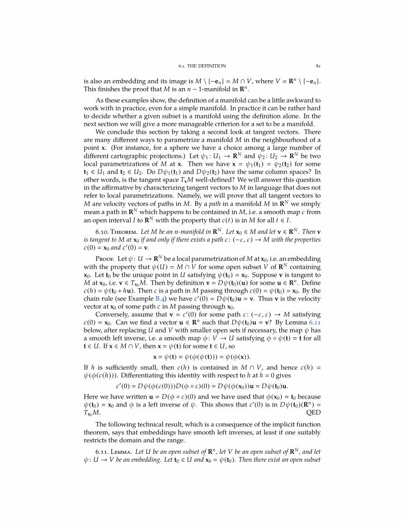
6.1. THE DEFINITION 81
is also an embedding and its image is M \ −en M ∩ V, where V Rn \ −en .This finishes the proof that M is an n − 1-manifold in Rn .
As these examples show, the definition of a manifold can be a little awkward towork with in practice, even for a simple manifold. In practice it can be rather hardto decide whether a given subset is a manifold using the definition alone. In thenext section we will give a more manageable criterion for a set to be a manifold.
We conclude this section by taking a second look at tangent vectors. Thereare many different ways to parametrize a manifold M in the neighbourhood of apoint x. (For instance, for a sphere we have a choice among a large number ofdifferent cartographic projections.) Let ψ1 : U1 → RN and ψ2 : U2 → RN be twolocal parametrizations of M at x. Then we have x ψ1(t1) ψ2(t2) for somet1 ∈ U1 and t2 ∈ U2. Do Dψ1(t1) and Dψ2(t2) have the same column spaces? Inother words, is the tangent space TxM well-defined? We will answer this questionin the affirmative by characterizing tangent vectors to M in language that does notrefer to local parametrizations. Namely, we will prove that all tangent vectors toM are velocity vectors of paths in M. By a path in a manifold M in RN we simplymean a path in RN which happens to be contained in M, i.e. a smooth map c froman open interval I to RN with the property that c(t) is in M for all t ∈ I.
6.10. Theorem. Let M be an n-manifold in RN . Let x0 ∈ M and let v ∈ RN . Then vis tangent to M at x0 if and only if there exists a path c : (−ε, ε) → M with the propertiesc(0) x0 and c′(0) v.
Proof. Letψ : U → RN be a local parametrization of M at x0, i.e. an embeddingwith the property that ψ(U) M ∩ V for some open subset V of RN containingx0. Let t0 be the unique point in U satisfying ψ(t0) x0. Suppose v is tangent toM at x0, i.e. v ∈ Tx0 M. Then by definition v Dψ(t0)(u) for some u ∈ Rn . Definec(h) ψ(t0 + hu). Then c is a path in M passing through c(0) ψ(t0) x0. By thechain rule (see Example B.4) we have c′(0) Dψ(t0)u v. Thus v is the velocityvector at x0 of some path c in M passing through x0.
Conversely, assume that v c′(0) for some path c : (−ε, ε) → M satisfyingc(0) x0. Can we find a vector u ∈ Rn such that Dψ(t0)u v? By Lemma 6.11below, after replacing U and V with smaller open sets if necessary, the map ψ hasa smooth left inverse, i.e. a smooth map φ : V → U satisfying φ ψ(t) t for allt ∈ U . If x ∈ M ∩ V, then x ψ(t) for some t ∈ U , so
x ψ(t) ψ(φ(ψ(t))) ψ(φ(x)).
If h is sufficiently small, then c(h) is contained in M ∩ V, and hence c(h)
ψ(φ(c(h))). Differentiating this identity with respect to h at h 0 gives
c′(0) Dψ(φ(c(0)))D(φ c)(0) Dψ(φ(x0))u Dψ(t0)u.
Here we have written u D(φ c)(0) and we have used that φ(x0) t0 becauseψ(t0) x0 and φ is a left inverse of ψ. This shows that c′(0) is in Dψ(t0)(Rn )
Tx0 M. QED
The following technical result, which is a consequence of the implicit functiontheorem, says that embeddings have smooth left inverses, at least if one suitablyrestricts the domain and the range.
6.11. Lemma. Let U be an open subset of Rn , let V be an open subset of RN , and letψ : U → V be an embedding. Let t0 ∈ U and x0 ψ(t0). Then there exist an open subset
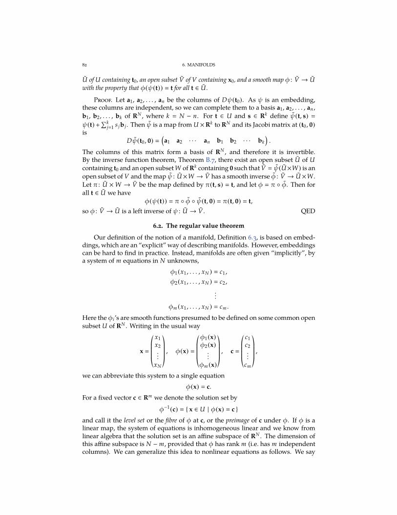
82 6. MANIFOLDS
U of U containing t0, an open subset V of V containing x0, and a smooth map φ : V → U
with the property that φ(ψ(t)) t for all t ∈ U .
Proof. Let a1, a2, . . . , an be the columns of Dψ(t0). As ψ is an embedding,these columns are independent, so we can complete them to a basis a1, a2, . . . , an ,b1, b2, . . . , bk of RN , where k N − n. For t ∈ U and s ∈ Rk define ψ(t, s)
ψ(t) +∑k
j1 s jb j . Then ψ is a map from U ×Rk to RN and its Jacobi matrix at (t0 , 0)
isDψ(t0 , 0)
(
a1 a2 · · · an b1 b2 · · · bk
)
.
The columns of this matrix form a basis of RN , and therefore it is invertible.By the inverse function theorem, Theorem B.7, there exist an open subset U of U
containing t0 and an open subset W of Rk containing 0 such that V ψ(U×W) is anopen subset of V and the map ψ : U×W → V has a smooth inverse φ : V → U×W .Let π : U ×W → V be the map defined by π(t, s) t, and let φ π φ. Then forall t ∈ U we have
φ(ψ(t)) π φ ψ(t, 0) π(t, 0) t,
so φ : V → U is a left inverse of ψ : U → V . QED
6.2. The regular value theorem
Our definition of the notion of a manifold, Definition 6.3, is based on embed-dings, which are an “explicit” way of describing manifolds. However, embeddingscan be hard to find in practice. Instead, manifolds are often given “implicitly”, bya system of m equations in N unknowns,
φ1(x1 , . . . , xN ) c1 ,
φ2(x1 , . . . , xN ) c2 ,
...
φm (x1 , . . . , xN ) cm .
Here the φi ’s are smooth functions presumed to be defined on some common opensubset U of RN . Writing in the usual way
x
*....,
x1
x2
...xN
+////-, φ(x)
*....,
φ1(x)
φ2(x)...
φm (x)
+////-, c
*....,
c1
c2
...cm
+////-,
we can abbreviate this system to a single equation
φ(x) c.
For a fixed vector c ∈ Rm we denote the solution set by
φ−1(c) x ∈ U | φ(x) c and call it the level set or the fibre of φ at c, or the preimage of c under φ. If φ is alinear map, the system of equations is inhomogeneous linear and we know fromlinear algebra that the solution set is an affine subspace of RN . The dimension ofthis affine subspace is N − m, provided that φ has rank m (i.e. has m independentcolumns). We can generalize this idea to nonlinear equations as follows. We say
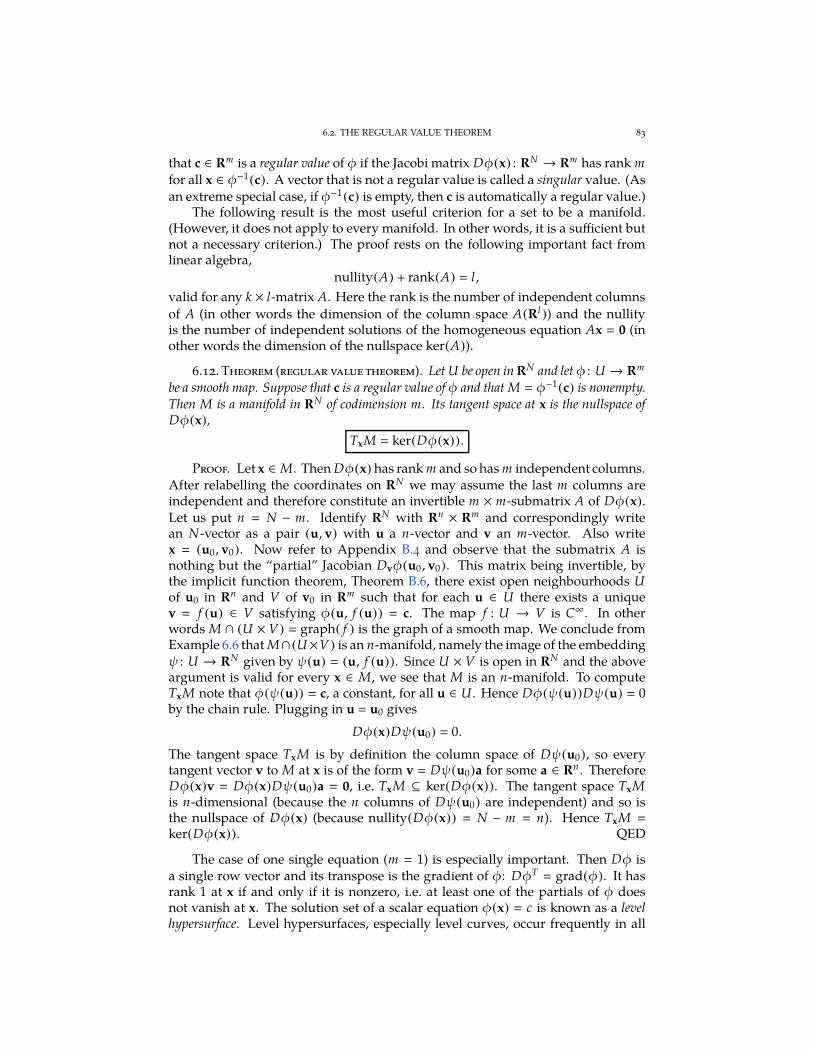
6.2. THE REGULAR VALUE THEOREM 83
that c ∈ Rm is a regular value of φ if the Jacobi matrix Dφ(x) : RN → Rm has rank m
for all x ∈ φ−1(c). A vector that is not a regular value is called a singular value. (Asan extreme special case, if φ−1(c) is empty, then c is automatically a regular value.)
The following result is the most useful criterion for a set to be a manifold.(However, it does not apply to every manifold. In other words, it is a sufficient butnot a necessary criterion.) The proof rests on the following important fact fromlinear algebra,
nullity(A) + rank(A) l,
valid for any k × l-matrix A. Here the rank is the number of independent columnsof A (in other words the dimension of the column space A(Rl )) and the nullityis the number of independent solutions of the homogeneous equation Ax 0 (inother words the dimension of the nullspace ker(A)).
6.12. Theorem (regular value theorem). Let U be open in RN and let φ : U → Rm
be a smooth map. Suppose that c is a regular value of φ and that M φ−1(c) is nonempty.Then M is a manifold in RN of codimension m. Its tangent space at x is the nullspace ofDφ(x),
TxM ker(Dφ(x)).
Proof. Let x ∈ M. Then Dφ(x) has rank m and so has m independent columns.After relabelling the coordinates on RN we may assume the last m columns areindependent and therefore constitute an invertible m × m-submatrix A of Dφ(x).Let us put n N − m. Identify RN with Rn × Rm and correspondingly writean N-vector as a pair (u, v) with u a n-vector and v an m-vector. Also writex (u0, v0). Now refer to Appendix B.4 and observe that the submatrix A isnothing but the “partial” Jacobian Dvφ(u0 , v0). This matrix being invertible, bythe implicit function theorem, Theorem B.6, there exist open neighbourhoods Uof u0 in Rn and V of v0 in Rm such that for each u ∈ U there exists a uniquev f (u) ∈ V satisfying φ(u, f (u)) c. The map f : U → V is C∞. In otherwords M ∩ (U × V) graph( f ) is the graph of a smooth map. We conclude fromExample 6.6 that M∩ (U×V) is an n-manifold, namely the image of the embeddingψ : U → RN given by ψ(u) (u, f (u)). Since U × V is open in RN and the aboveargument is valid for every x ∈ M, we see that M is an n-manifold. To computeTxM note that φ(ψ(u)) c, a constant, for all u ∈ U . Hence Dφ(ψ(u))Dψ(u) 0by the chain rule. Plugging in u u0 gives
Dφ(x)Dψ(u0) 0.
The tangent space TxM is by definition the column space of Dψ(u0), so everytangent vector v to M at x is of the form v Dψ(u0)a for some a ∈ Rn . ThereforeDφ(x)v Dφ(x)Dψ(u0)a 0, i.e. TxM ⊆ ker(Dφ(x)). The tangent space TxMis n-dimensional (because the n columns of Dψ(u0) are independent) and so isthe nullspace of Dφ(x) (because nullity(Dφ(x)) N − m n). Hence TxM
ker(Dφ(x)). QED
The case of one single equation (m 1) is especially important. Then Dφ isa single row vector and its transpose is the gradient of φ: DφT
grad(φ). It hasrank 1 at x if and only if it is nonzero, i.e. at least one of the partials of φ doesnot vanish at x. The solution set of a scalar equation φ(x) c is known as a levelhypersurface. Level hypersurfaces, especially level curves, occur frequently in all
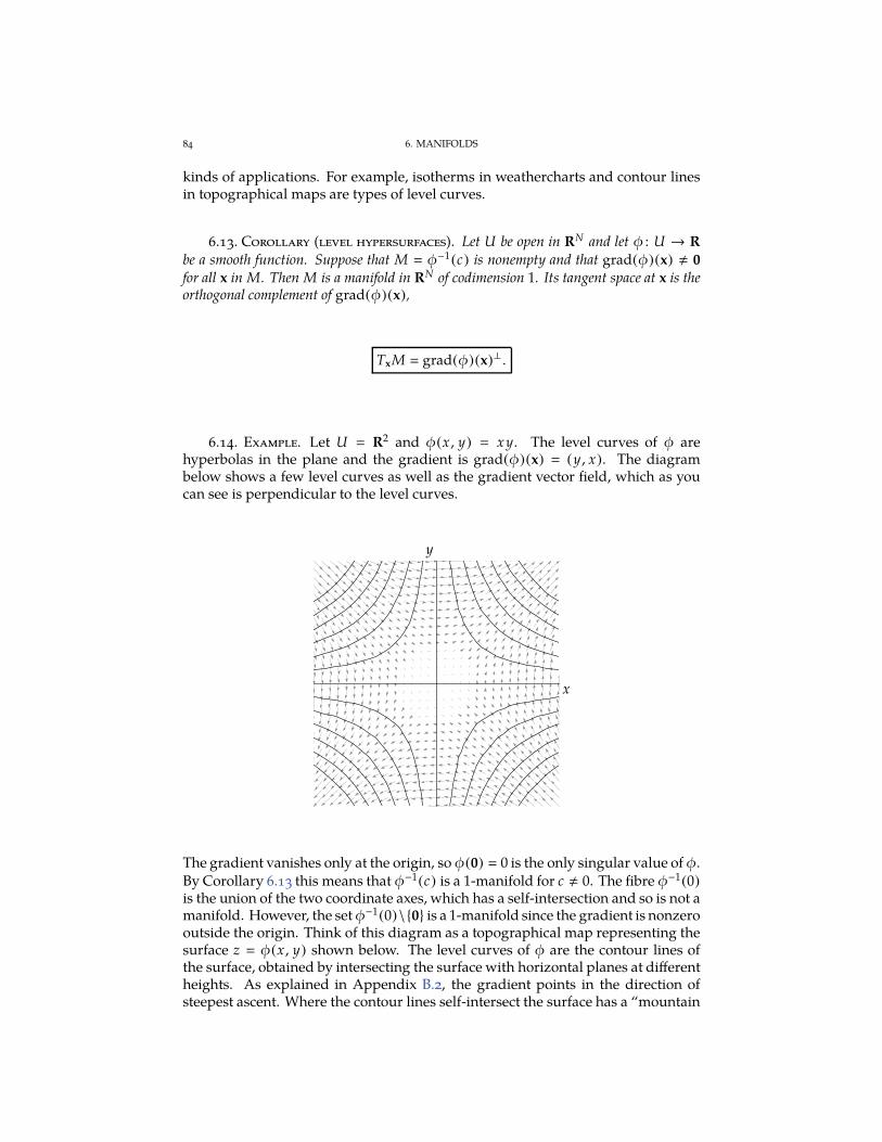
84 6. MANIFOLDS
kinds of applications. For example, isotherms in weathercharts and contour linesin topographical maps are types of level curves.
6.13. Corollary (level hypersurfaces). Let U be open in RN and let φ : U → R
be a smooth function. Suppose that M φ−1(c) is nonempty and that grad(φ)(x) , 0
for all x in M. Then M is a manifold in RN of codimension 1. Its tangent space at x is theorthogonal complement of grad(φ)(x),
TxM grad(φ)(x)⊥ .
6.14. Example. Let U R2 and φ(x , y) x y. The level curves of φ arehyperbolas in the plane and the gradient is grad(φ)(x) (y , x). The diagrambelow shows a few level curves as well as the gradient vector field, which as youcan see is perpendicular to the level curves.
x
y
The gradient vanishes only at the origin, so φ(0) 0 is the only singular value of φ.By Corollary 6.13 this means that φ−1(c) is a 1-manifold for c , 0. The fibre φ−1(0)
is the union of the two coordinate axes, which has a self-intersection and so is not amanifold. However, the set φ−1(0)\0 is a 1-manifold since the gradient is nonzerooutside the origin. Think of this diagram as a topographical map representing thesurface z φ(x , y) shown below. The level curves of φ are the contour lines ofthe surface, obtained by intersecting the surface with horizontal planes at differentheights. As explained in Appendix B.2, the gradient points in the direction ofsteepest ascent. Where the contour lines self-intersect the surface has a “mountain
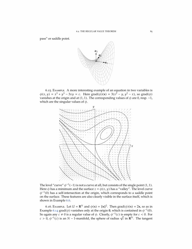
6.2. THE REGULAR VALUE THEOREM 85
pass” or saddle point.
e1
e2
e3
6.15. Example. A more interesting example of an equation in two variables isφ(x , y) x3 + y3 − 3x y c. Here grad(φ)(x) 3(x2 − y , y2 − x), so grad(φ)
vanishes at the origin and at (1, 1). The corresponding values of φ are 0, resp. −1,which are the singular values of φ.
x
y
The level “curve”φ−1(−1) is not a curve at all, but consists of the single point (1, 1).Here φ has a minimum and the surface z φ(x , y) has a “valley”. The level curveφ−1(0) has a self-intersection at the origin, which corresponds to a saddle pointon the surface. These features are also clearly visible in the surface itself, which isshown in Example 6.6.
6.16. Example. Let U RN and φ(x) ‖x‖2. Then grad(φ)(x) 2x, so as inExample 6.14 grad(φ) vanishes only at the origin 0, which is contained in φ−1(0).So again any c , 0 is a regular value of φ. Clearly, φ−1(c) is empty for c < 0. Forc > 0, φ−1(c) is an N − 1-manifold, the sphere of radius
√c in RN . The tangent
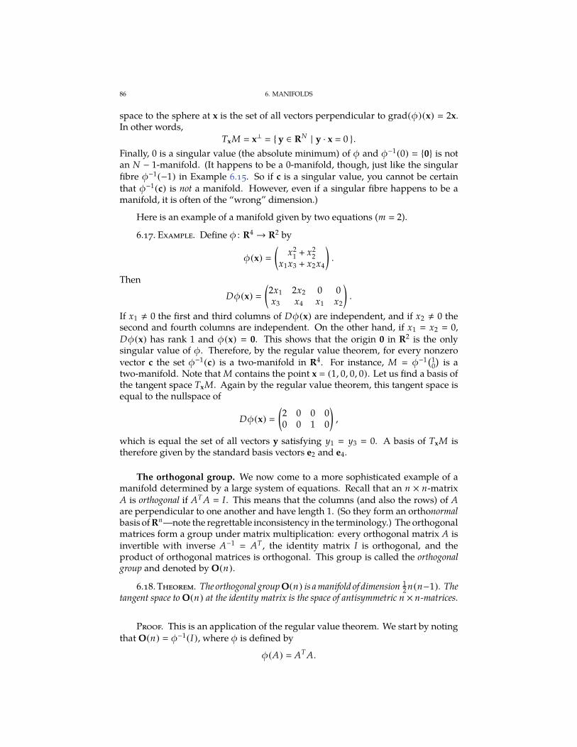
86 6. MANIFOLDS
space to the sphere at x is the set of all vectors perpendicular to grad(φ)(x) 2x.In other words,
TxM x⊥ y ∈ RN | y · x 0 .Finally, 0 is a singular value (the absolute minimum) of φ and φ−1(0) 0 is notan N − 1-manifold. (It happens to be a 0-manifold, though, just like the singularfibre φ−1(−1) in Example 6.15. So if c is a singular value, you cannot be certainthat φ−1(c) is not a manifold. However, even if a singular fibre happens to be amanifold, it is often of the “wrong” dimension.)
Here is an example of a manifold given by two equations (m 2).
6.17. Example. Define φ : R4 → R2 by
φ(x)
(
x21
+ x22
x1x3 + x2x4
)
.
Then
Dφ(x)
(
2x1 2x2 0 0x3 x4 x1 x2
)
.
If x1 , 0 the first and third columns of Dφ(x) are independent, and if x2 , 0 thesecond and fourth columns are independent. On the other hand, if x1 x2 0,Dφ(x) has rank 1 and φ(x) 0. This shows that the origin 0 in R2 is the onlysingular value of φ. Therefore, by the regular value theorem, for every nonzerovector c the set φ−1(c) is a two-manifold in R4. For instance, M φ−1 (1
0
)
is atwo-manifold. Note that M contains the point x (1, 0, 0, 0). Let us find a basis ofthe tangent space TxM. Again by the regular value theorem, this tangent space isequal to the nullspace of
Dφ(x)
(
2 0 0 00 0 1 0
)
,
which is equal the set of all vectors y satisfying y1 y3 0. A basis of TxM istherefore given by the standard basis vectors e2 and e4.
The orthogonal group. We now come to a more sophisticated example of amanifold determined by a large system of equations. Recall that an n × n-matrixA is orthogonal if ATA I. This means that the columns (and also the rows) of Aare perpendicular to one another and have length 1. (So they form an orthonormalbasis of Rn—note the regrettable inconsistency in the terminology.) The orthogonalmatrices form a group under matrix multiplication: every orthogonal matrix A isinvertible with inverse A−1
AT , the identity matrix I is orthogonal, and theproduct of orthogonal matrices is orthogonal. This group is called the orthogonalgroup and denoted by O(n).
6.18. Theorem. The orthogonal group O(n) is a manifold of dimension 12 n(n−1). The
tangent space to O(n) at the identity matrix is the space of antisymmetric n × n-matrices.
Proof. This is an application of the regular value theorem. We start by notingthat O(n) φ−1(I), where φ is defined by
φ(A) ATA.
6.2. THE REGULAR VALUE THEOREM 87
The domain of the map φ is V Rn×n , the vector space of all n × n-matrices. Wecan regard φ as a map from V to itself, but then the identity matrix I is not a regularvalue! To ensure that I is a regular value we must restrict the range of φ. This isdone by observing that (ATA)T
ATA, so ATA is a symmetric matrix. In otherwords, if we let W C ∈ V | C CT be the linear subspace of V consisting ofall symmetric matrices, then we can regard φ as a map
φ : V −→ W.
We will show that I is a regular value of this map. To do this we need to computethe total derivative of φ. For every matrix A ∈ V the total derivative at A is a linearmap Dφ(A) : V → W , which can be computed by using Lemma B.1. This lemmasays that for every B ∈ V the result of applying the linear map Dφ(A) to B is thedirectional derivative of φ at A along B:
Dφ(A)B limt→0
1
t(φ(A + tB) − φ(A))
limt→0
1
t(ATA + tAT B + tBTA + t2BT B − ATA)
ATB + BTA.
We need to show that for all A ∈ O(n) the linear map Dφ(A) : V →W is surjective.This amounts to showing that, given any orthogonal A and any symmetric C, theequation
ATB + BTA C (6.1)is solvable for B. Here is a trick for guessing a solution: observe that C
12 (C + CT )
and first try to solve AT B 12 C. Left multiplying both sides by A and using AAT
I
gives B 12 AC. We claim that B
12 AC is a solution of equation (6.1). Indeed,
AT B + BTA AT 1
2AC +
1
2CTATA
1
2(C + CT ) C.
By the regular value theorem this proves that O(n) is a manifold. You will beasked to prove the remaining assertions in Exercise 6.12. QED
If A is an orthogonal matrix, then det(ATA) det(I) 1, so (det(A))2 1, i.e.
det(A) ±1. The special orthogonal group or rotation group is
SO(n) A ∈ O(n) | det(A) 1 .If A and B are elements of O(n) that are not in SO(n), then AB ∈ O(n) anddet(AB) det(A) det(B) 1, so AB ∈ SO(n). An example of an orthogonalmatrix which is not a rotation is a reflection matrix, such as
A0
*....,
−1 0 · · · 00 1 · · · 0...
.... . .
...0 0 · · · 1
+////-.
Every orthogonal matrix A which is not in SO(n) can be written as A A0C fora unique C ∈ SO(n), namely C A0A. Thus we see that O(n) is a union of twodisjoint pieces,
O(n) SO(n) ∪ A0C | C ∈ SO(n) ,each of which is a manifold of dimension 1
2 n(n − 1).
88 6. MANIFOLDS
In two dimenson the rotation group is the group SO(2) of all matrices of theform (
cos θ − sin θsin θ cos θ
)
.
As a manifold SO(2) is a copy of the unit circle S1. The rotation group in threedimensions SO(3) is a three-dimensional manifold, which is a little harder tovizualize. Every rotation can be parametrized by a vector x ∈ R3, namely as therotation about the axis spanned by x through an angle of ‖x‖ radians. But SO(3)
is not the same as R3, because many different vectors represent the same rotation.Every rotation can be represented by a vector of length ≤ π, so let us restrict xto the (solid) ball B of radius π about the origin. This gets rid of most of theambiguity, except for the fact that two antipodal points on the boundary sphererepresent the same rotation (because rotation through π about a given axis is thesame as rotation through −π). We conclude that SO(3) is the manifold obtainedby identifying opposite points on the boundary of B. This is the three-dimensionalprojective space.
Exercises
6.1. This is a continuation of Exercise 1.1. Define ψ : R → R2 by ψ(t) (t − sin t , 1 −cos t). Show that ψ is one-to-one. Determine all t for which ψ′(t) 0. Prove that ψ(R) isnot a manifold at these points.
6.2. Let a ∈ (0, 1) be a constant. Prove that the map ψ : R → R2 given by ψ(t)
(t − a sin t , 1− a cos t) is an embedding. (This becomes easier if you first show that t − a sin tis an increasing function of t.) Graph the curve defined by ψ.
6.3. Prove that the mapψ : R→ R2 given byψ(t) 12 (e t +e−t , e t−e−t ) is an embedding.
Conclude that M ψ(R) is a 1-manifold. Graph the curve M. Compute the tangent line toM at (1, 0) and try to find an equation for M.
6.4. Let I be the open interval (−1,∞) and let ψ : I → R2 be the map ψ(t) (3at/(1 +
t3 , 3at2/(1+t3)), where a is a nonzero constant. Show that ψ is one-to-one and that ψ′(t) , 0for all t ∈ I. Is ψ an embedding and is ψ(I) a manifold? (Observe that ψ(I) is a portion ofthe curve studied in Exercise 1.2.)
6.5. Define ψ : R→ R2 by
ψ(t)
(− f (t), f (t))
if t ≤ 0,(
f (t), f (t))
if t ≥ 0,
where f is the function given in Exercise B.3. Show that ψ is smooth, one-to-one and that
its inverse ψ−1 : ψ(R) → R is continuous. Sketch the image of ψ. Is ψ(R) a manifold?
6.6. Define a map ψ : R2 → R4 by ψ(t1 , t2) (
t31, t2
1t2 , t1t2
2, t3
2
)
.
(i) Show that ψ is one-to-one.(ii) Show that Dψ(t) is one-to-one for all t , 0.
(iii) Let U be the punctured plane R2 \ 0. Show that ψ : U → R4 is an embedding.
Conclude that ψ(U) is a two-manifold in R4.(iv) Find a basis of the tangent plane to ψ(U) at the point ψ(1, 1).
6.7. (i) Let U be an open subset of Rn and let ψ : U → RN be a smooth map.
The tangent map of ψ is the map Tψ : U × Rn → R2N defined by Tψ(t, u) (
ψ(t),Dψ(t)u)
for t ∈ U and u ∈ Rn . Prove that the tangent map of an embed-ding is an embedding.
EXERCISES 89
(ii) Let M be an n-manifold in RN . The tangent bundle of M is the subset TM of R2N
defined by
TM (x, v) ∈ R2N | v ∈ TxM .Prove that the tangent bundle of M is a 2n-manifold.
6.8. Let M be the set of points in R2 given by the equation (x2 + y2)2 + y2 − x2 0.
(i) Show that M \ (0, 0) is a 1-manifold.(ii) Determine the points where M has horizontal or vertical tangent lines.
(iii) Sketch M. (Start by finding the intersection points of M with an arbitrary linethrough the origin, y ax.)
(iv) Is M a manifold at (0, 0)? Explain.
6.9. Let φ : Rn \ 0 → R be a homogeneous function of degree p as defined in ExerciseB.6. Assume that φ is smooth and that p , 0. Show that 0 is the only possible singular value
of φ. (Use the result of Exercise B.6.) Conclude that, if nonempty, φ−1(c) is an n−1-manifoldfor c , 0.
6.10. Let φ(x) a1x21
+a2x22
+ · · ·+an x2n , where the ai are nonzero constants. Determine
the regular and singular values of φ. For n 3 sketch the level surface φ−1(c) for a regularvalue c. (You have to distinguish between a few different cases.)
6.11. Show that the trajectories of the Lotka-Volterra system of Exercise 1.11 are one-dimensional manifolds.
6.12. Let V be the vector space of n × n-matrices and let W be its linear subspaceconsisting of all symmetric matrices.
(i) Prove that dim(V ) n2 and dim(W ) 12 n(n + 1). (Exhibit explicit bases of V
and W , and count the number of elements in each basis.)(ii) Compute the dimension of the orthogonal group O(n) and show that its tangent
space at the identity matrix I is the set of all antisymmetric n × n-matrices. (Usethe regular value theorem, which says that the dimension of O(n) is dim(V ) −dim(W ) and that the tangent space at the identity matrix is the kernel of Dφ(I),
where φ : V →W is defined by φ(A) AT A. See the proof of Theorem 6.18.)
6.13. Let V be the vector space of n × n-matrices.
(i) The general linear group is the subset of V defined by
GL(n) A ∈ V | det(A) , 0 .Show that GL(n) is a manifold. What is its dimension?
(ii) Define φ : V → R by φ(A) det(A). Show that
Dφ(A)B
n∑
i1
det(a1 , a2 , . . . , ai−1 , bi , ai+1 , . . . , an ),
where a1, a2 , . . . , an and b1, b2 , . . . , bn denote the column vectors of A, resp. B.(Apply Lemma B.1 for the derivative and use the multilinearity of the determi-nant.)
(iii) The special linear group is the subset of V defined by
SL(n) A ∈ V | det(A) 1 .Show that SL(n) is a manifold. What is its dimension?
(iv) Show that for A I, the identity matrix, we have Dφ(A)B
∑ni1
bi ,i tr(B),the trace of B. Conclude that the tangent space to SL(n) at I is the set of tracelessmatrices, i.e. matrices B satisfying tr(B) 0.
90 6. MANIFOLDS
6.14. (i) Let W be punctured 4-space R4 \ 0 and define φ : W → R by
φ(x) x1x4 − x2x3 .
Show that 0 is a regular value of φ.(ii) Let A be a real 2× 2-matrix. Show that rank(A) 1 if and only if det(A) 0 and
A , 0.(iii) Let M be the set of 2 × 2-matrices of rank 1. Show that M is a three-dimensional
manifold.(iv) Compute TAM, where A
(1 10 0
)
.
6.15. Define φ : R4 → R2 by φ(x) (x1 + x2 + x3x4 , x1x2x3 + x4).
(i) Show that Dφ(x) has rank 2 unless x is of the form (t−2 , t−2 , t , t−3) for somet , 0. (Row reduce the matrix Dφ(x) to compute its rank.)
(ii) Show that M φ−1(0) is a 2-manifold (where 0 is the origin in R2).(iii) Find a basis of the tangent space TxM for all x ∈ M with x3 0. (The answer
depends on x.)
6.16. Let U be an open subset of Rn and let φ : U → Rm be a smooth map. Let M be
the manifold φ−1(c), where c is a regular value of φ. Let f : U → R be a smooth function. Apoint x ∈ M is called a critical point for the restricted function f |M if D f (x)v 0 for all tangentvectors v ∈ TxM. Prove that x ∈ M is critical for f |M if and only if there exist numbers λ1,λ2 , . . . , λm such that
grad( f )(x) λ1 grad(φ1)(x) + λ2 grad(φ2)(x) + · · · + λm grad(φm )(x).
(Use the characterization of TxM given by the regular value theorem.)
6.17. Find the critical points of the function f (x, y , z) −x + 2y + 3z over the circle Cgiven by
x2 + y2 + z2 1,
x + z 0.
Where are the maxima and minima of f |C?
6.18 (eigenvectors via calculus). Let A AT be a symmetric n × n-matrix and definef : Rn → R by f (x) x · Ax. Let M be the unit sphere x ∈ Rn | ‖x‖ 1 .
(i) Calculate grad( f )(x).(ii) Show that x ∈ M is a critical point of f |M if and only if x is an eigenvector for A
of length 1.(iii) Given an eigenvector x of length 1, show that f (x) is the corresponding eigenvalue
of x.
CHAPTER 7
Differential forms on manifolds
7.1. First definition
There are several different ways to define differential forms on manifolds.In this section we present a practical, workaday definition. A more theoreticalapproach is taken in Section 7.2.
Let M be an n-manifold in RN and let us first consider what we might mean bya 0-form or smooth function on M. A function f : M → R is simply an assignmentof a unique number f (x) to each point x in M. For instance, M could be thesurface of the earth and f could represent temperature at a given time, or heightabove sea level. But how would we define such a function to be differentiable?The difficulty here is that if x is in M and e j is one of the standard basis vectors,the straight line x + te j may not be contained in M, so we cannot form the limit∂ f /∂x j limt→0( f (x + te j) − f (x))/t.
Here is one way out of this difficulty. Because M is a manifold there exist opensets Ui in Rn and embeddings ψi : Ui → RN such that the images ψi (Ui ) cover M:M
⋃
i ψi (Ui ). (Here i ranges over some unspecified, possibly infinite, index set.)For each i we define a function fi : Ui → R by fi (t) f (ψi (t)), i.e. fi ψ∗i ( f ). Wecall fi the local representative of f relative to the embedding ψi . (For instance, if Mis the earth’s surface, f is temperature, and ψi is a map of New York State, then fi
represents a temperature chart of NY.) Since fi is defined on the open subset Ui ofRn , it makes sense to ask whether its partial derivatives exist. We say that f is Ck ifeach of the local representatives fi is Ck . Now suppose that x is in the overlap of twocharts. Then we have two indices i and j and vectors t ∈ Ui and u ∈ U j such thatx ψi (t) ψ j (u). Then we must have f (x) f (ψi (t)) f (ψ j (u)), so fi (t) f j (u).Also ψi (t) ψ j (u) implies t ψ−1
i ψ j (u) and therefore f j (u) fi
(
ψ−1i ψ j (u)
)
.This identity must hold for all u ∈ U j such that ψ j (u) ∈ ψi (Ui), i.e. for all u inψ−1
j(ψi (Ui)). We can abbreviate this by saying that
f j (ψ−1i ψ j )
∗( fi )
on ψ−1j
(ψi (Ui )). This is a consistency condition on the functions fi imposed bythe fact that they are pullbacks of a single function f defined everywhere onM. The map ψ−1
i ψ j is often called a change of coordinates or transition map,
and the consistency condition is also known as the transformation law for the localrepresentatives fi . (Pursuing the weather chart analogy, it expresses nothing butthe obvious fact that where the maps of New York and Pennsylvania overlap,the corresponding two temperature charts must show the same temperatures.)Conversely, the collection of all local representatives fi determines f , because we
91
92 7. DIFFERENTIAL FORMS ON MANIFOLDS
have f (x) fi (ψ−1i
(x)) if x ∈ ψi (Ui). (That is to say, if we have a complete set ofweather charts for the whole world, we know the temperature everywhere.)
Following this cue we formulate the following definition.
7.1. Definition. A differential form of degree k, or simply a k-form, α on M is acollection of k-forms αi on Ui satisfying the transformation law
α j (ψ−1i ψ j )
∗(αi ) (7.1)
on ψ−1j
(ψi (Ui )). We call αi the local representative of α relative to the embeddingψi and denote it by αi ψ∗i (α). The collection of all k-forms on M is denoted byΩk (M).
This definition is rather indirect, but it works really well if a specific atlas forthe manifold M is known. Definition 7.1 is particularly tractible if M is the imageof a single embedding ψ : U → RN . In that case the compatibility relation (7.1) isvacuous and a k-form α on M is determined by one single representative, a k-formψ∗(α) on U .
Sometimes it is useful to write the transformation law (7.1) in components. Ap-pealing to Theorem 3.13 we see that (7.1) is equivalent to the following requirement:if
αi
∑
I
fI dtI and α j
∑
J
g J dt J
are two local representatives for α, then
g J
∑
I
(ψ−1i ψ j )
∗ ( fI det(D(ψ−1i ψ j )I ,J )
)
.
on ψ−1j
(ψi (Ui )).Just like forms on Rn , forms on a manifold can be added, multiplied, differ-
entiated and integrated. For example, suppose α is a k-form and β an l-form onM. Suppose αi , resp. βi , is the local representative of α, resp. β, relative to anembedding ψi : Ui → M. Then we define the product γ αβ by setting γi αiβi .To see that this definition makes sense, we check that the forms γi satisfy thetransformation law (7.1):
γj α jβ j (ψ−1i ψ j )
∗(αi )(ψ−1i ψ j )
∗(βi ) (ψ−1i ψ j )
∗(αiβi ) (ψ−1i ψ j )
∗(γi ).
Here we have used the multiplicative property of pullbacks, Proposition 3.10(ii).Similarly, the exterior derivative of α is defined by setting (dα)i dαi . As before,let us check that the forms (dα)i satisfy the transformation law (7.1):
(dα) j dα j d(ψ−1i ψ j )
∗(αi ) (ψ−1i ψ j )
∗(dαi ) (ψ−1i ψ j )
∗((dα)i ),
where we used Theorem 3.11.
7.2. Second definition
This section presents some of the algebraic underpinnings of the theory ofdifferential forms. This branch of algebra, now called exterior or alternating algebrawas invented by Grassmann in the mid-nineteenth century and is a prerequisitefor much of the more advanced literature on the subject.
7.2. SECOND DEFINITION 93
Covectors. A covector is a little dinosaur that eats vectors and spits out num-bers, in a linear way.
The formal definition goes as follows. Let V be a vector space over the realnumbers, for example Rn or a linear subspace of Rn . A covector, or dual vector, orlinear functional, is a linear map from V to R.
7.2. Example. Let V C0([a, b],R), the collection of all continuous real-valuedfunctions on a closed and bounded interval [a, b]. A linear combination of con-tinuous functions is continuous, so V is a vector space. Define µ( f )
∫ b
a f (x) dx.Then µ(c1 f1 + c2 f2) c1µ( f1) + c2µ( f2) for all functions f1, f2 ∈ V and all scalarsc1, c2, so µ is a linear functional on V.
The collection of all covectors on V is denoted by V∗ and called the dual of V.The dual is a vector space in its own right: if µ1 and µ2 are in V∗ we define µ1 + µ2
and cµ1 by setting (µ1 +µ2)(v) µ1(v) +µ2(v) and (cµ1)(v) cµ1(v) for all v ∈ V.For the next example, recall that if A is an m × n-matrix and x an n-vector, then
Ax is an m-vector, and the map which sends x to Ax is linear. Moreover, everylinear map from Rn to Rm is of this form for a unique matrix A.
7.3. Example. A covector on Rn is a linear map from Rn to R R1 and istherefore given by a 1 × n-matrix, which is nothing but a row vector. Thus (Rn)∗
is the space of row n-vectors. A row vector y “eating” a column vector x meansmultiplying the two, which results in a number:
yx
(
y1 y2 · · · yn
)*....,
x1
x2
...xn
+////-
n∑
i1
yixi .
Now suppose that V is a vector space of finite dimension n and choose a basisb1, b2 , . . . , bn of V. Then every vector b ∈ V can be written in a unique way asa linear combination
∑
j c jb j . Define a covector βi ∈ V∗ by βi (b) ci . In otherwords, βi is determined by the rule βi (b j ) δi , j , where
δi , j
1 if i j ,
0 if i , j
is the Kronecker delta. We call βi the i-th coordinate function.
7.4. Lemma. The coordinate functions β1, β2 , . . . , βn form a basis of V∗. It followsthat dim(V∗) n dim(V).
Proof. Let β ∈ V∗. We need to prove that β can be written as a linear combina-tion β
∑ni1 ciβi with unique coefficients ci . First we prove uniqueness. Assuming
94 7. DIFFERENTIAL FORMS ON MANIFOLDS
that β can be expressed as β
∑ni1 ciβi , we can apply both sides to the vector b j to
obtain
β(b j )
n∑
i1
ciβi (b j )
n∑
i1
ciδi , j c j . (7.2)
So c j β(b j ) is the only possible choice for the coefficient c j . This argumentestablishes the uniqueness of the coefficients. Moreover, it tells us what the co-efficients should be, which helps us prove that they exist. Namely, let us defineβ′
∑ni1 β(bi )βi . Then by equation (7.2), β′(b j ) β(b j ) for all j, so β′ β, and
therefore β
∑ni1 β(bi )βi . This proves that β1, β2 , . . . , βn constitute a basis of V∗.
The cardinality of the basis is n, so dim(V∗) n. QED
The basis β1, β2 , . . . , βn of V∗ is said to be dual to the basis b1, b2, . . . , bn ofV.
7.5. Example. Let b1, b2, . . . , bn be a basis of Rn . What is the dual basisβ1, β2 , . . . , βn of (Rn)∗? The βi ’s are row vectors determined by the equationsβib j δi , j . These equations can be written as a single matrix equation: let B bethe n × n-matrix with columns b1, b2, . . . , bn and let A be the n × n-matrix withrows β1, β2 , . . . , βn ; then AB I. Therefore A is the inverse of B. In other words,βi is the i-th row of B−1. As a special case consider the standard basis e1, . . . , en .Then B I, so A I, and the dual basis of (Rn )∗ is eT
1, eT
2, . . . , eT
n .
Dual bases come in handy when writing the matrix of a linear map. LetL : V → W be a linear map between vector spaces V and W . To write the matrixof L we need to start by picking a basis b1, b2, . . . , bn of V and a basis c1, c2, . . . ,cm of W . Then for each j 1, 2, . . . , n the vector Lb j can be expanded uniquely interms of the c’s: Lb j
∑mi1 li , jci . The m × n numbers li , j make up the matrix of L
relative to the two bases of V and W .
7.6. Lemma. Let γ1, γ2 , . . . , γm ∈ W∗ the dual basis of c1, c2, . . . , cm . Then the(i, j)-th matrix element of a linear map L : V →W is equal to li , j γi (Lb j ).
Proof. We have Lb j ∑m
k1 lk , jck , so
γi (Lb j )
m∑
k1
lk , jγi (ck )
m∑
k1
lk , jδi ,k li , j ,
that is to say li , j γi (Lb j ). QED
1-Forms on Rn re-examined. Let U be an open subset of Rn . Recall that avector field on U is a smooth map F : U → Rn . A 1-form is a type of object “dual”to a vector field. Formally, a 1-form or covector field on U is defined as a smooth mapα : U → (Rn)∗. This means that α is a row vector
α ( f1 f2 · · · fn )
whose entries are smooth functions on U . The form is called constant if the entriesf1 , . . . , fn are constant. By definition dxi is the constant 1-form
dxi eTi (0 · · · 0 1 0 · · · 0), (7.3)
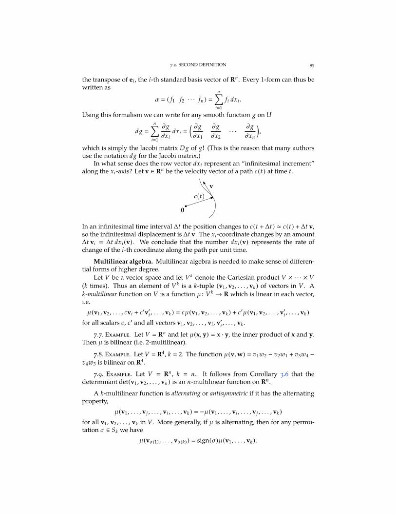
7.2. SECOND DEFINITION 95
the transpose of ei, the i-th standard basis vector of Rn . Every 1-form can thus bewritten as
α ( f1 f2 · · · fn )
n∑
i1
fi dxi .
Using this formalism we can write for any smooth function g on U
dg
n∑
i1
∂g
∂xidxi
( ∂g
∂x1
∂g
∂x2· · ·
∂g
∂xn
)
,
which is simply the Jacobi matrix D g of g! (This is the reason that many authorsuse the notation dg for the Jacobi matrix.)
In what sense does the row vector dxi represent an “infinitesimal increment”along the xi-axis? Let v ∈ Rn be the velocity vector of a path c(t) at time t.
0
c(t)
v
In an infinitesimal time interval ∆t the position changes to c(t + ∆t) ≈ c(t) + ∆t v,so the infinitesimal displacement is ∆t v. The xi-coordinate changes by an amount∆t vi ∆t dxi (v). We conclude that the number dxi (v) represents the rate ofchange of the i-th coordinate along the path per unit time.
Multilinear algebra. Multilinear algebra is needed to make sense of differen-tial forms of higher degree.
Let V be a vector space and let Vk denote the Cartesian product V × · · · × V
(k times). Thus an element of Vk is a k-tuple (v1 , v2 , . . . , vk ) of vectors in V. Ak-multilinear function on V is a function µ : Vk → R which is linear in each vector,i.e.
µ(v1 , v2, . . . , cvi + c′v′i , . . . , vk ) cµ(v1 , v2, . . . , vk ) + c′µ(v1 , v2, . . . , v′i , . . . , vk )
for all scalars c, c′ and all vectors v1, v2 , . . . , vi , v′i, . . . , vk .
7.7. Example. Let V Rn and let µ(x, y) x · y, the inner product of x and y.Then µ is bilinear (i.e. 2-multilinear).
7.8. Example. Let V R4, k 2. The function µ(v,w) v1w2 − v2w1 + v3w4 −v4w3 is bilinear on R4.
7.9. Example. Let V Rn , k n. It follows from Corollary 3.6 that thedeterminant det(v1 , v2, . . . , vn) is an n-multilinear function on Rn .
A k-multilinear function is alternating or antisymmetric if it has the alternatingproperty,
µ(v1 , . . . , v j , . . . , vi , . . . , vk ) −µ(v1 , . . . , vi , . . . , v j , . . . , vk )
for all v1, v2 , . . . , vk in V. More generally, if µ is alternating, then for any permu-tation σ ∈ Sk we have
µ(vσ(1) , . . . , vσ(k)) sign(σ)µ(v1 , . . . , vk ).
96 7. DIFFERENTIAL FORMS ON MANIFOLDS
7.10. Example. The inner product of Example 7.7 is bilinear, but it is not alter-nating. Indeed it is symmetric: y · x x · y. The bilinear function of Example 7.8 isalternating, and so is the determinant function of Example 7.9.
Here is a useful trick for producing alternating k-multilinear functions startingfrom k covectors µ1, µ2, . . . , µk ∈ V∗. The (wedge) product is the function
µ1µ2 · · · µk : Vk → R
defined by
µ1µ2 · · · µk (v1 , v2 , . . . , vk ) det(
µi (v j ))
1≤i , j≤k .
(The determinant on the right is a k × k-determinant.) It follows from the mul-tilinearity and the alternating property of the determinant that µ1µ2 · · · µk is analternating k-multilinear function. Some authors denote the wedge product byµ1 ∧ µ2 ∧ · · · ∧ µk to distinguish it from other products, such as the tensor productdefined in Exercise 7.6.
The collection of all alternating k-multilinear functions is denoted by Ak (V).For any k, k-multilinear functions can be added and scalar-multiplied just likeordinary linear functions, so the set Ak (V) forms a vector space.
For k 1 the alternating property is vacuous, so an alternating 1-multilinearfunction is nothing but a linear function. Thus A1(V) V∗.
A 0-multilinear function is by convention just a number. Thus A0(V) R.There is a nice way to construct a basis of the vector space Ak (V) starting from
a basis b1, . . . , bn of V. The idea is to take wedge products of dual basis vectors.Let β1 , . . . , βn be the corresponding dual basis of V∗. Let I (i1 , i2 , . . . , ik ) be anincreasing multi-index, i.e. 1 ≤ i1 < i2 < · · · < ik ≤ n. Write
βI βi1βi2 · · · βik ∈ Ak (V),
bI (bi1 , bi2 , . . . , bik ) ∈ Vk .
7.11. Example. Let V R3 with standard basis e1, e2, e3. The dual basis of(R3)∗ is dx1 , dx2, dx3. Let k 2 and I (1, 2), J (2, 3). Then
dxI (eI ) dx1(e1) dx1(e2)
dx2(e1) dx2(e2)
1 00 1
1,
dxI (eJ ) dx1(e2) dx1(e3)
dx2(e2) dx2(e3)
0 01 0
0,
dx J (eI ) dx2(e1) dx2(e2)
dx3(e1) dx3(e2)
0 10 0
0,
dx J (eJ ) dx2(e2) dx2(e3)
dx3(e2) dx3(e3)
1 00 1
1.
This example generalizes as follows. For multi-indices I and J let us define ageneralized Kronecker delta δI ,J by
δI ,J
1 if I J ,
0 if I , J .
7.12. Lemma. Let I and J be increasing multi-indices of degree k. Then βI (bJ ) δI ,J .
7.2. SECOND DEFINITION 97
Proof. Let I (i1 , . . . , ik ) and J ( j1 , . . . , jk ). Then
βI (bJ ) det(
βir (b js ))
1≤r,s≤k
δi1 , j1 . . . δi1 , jk...
...δil , j1 . . . δil , jk...
...δik , j1 . . . δik , jk
.
If I J , then this matrix is the identity k×k-matrix, so βI (bJ ) 1. If I , J , then thereis some i ∈ I which is not in J , say i il , which causes all entries in the l-th row ofthe matrix to vanish. Hence its determinant is 0, and therefore βI (bJ ) 0. QED
We need one further technical result before showing that the functions βI area basis of Ak (V).
7.13. Lemma. Let β ∈ Ak (V). Suppose β(bI ) 0 for all increasing multi-indices Iof degree k. Then β 0.
Proof. The assumption implies
β(bi1 , . . . , bik ) 0 (7.4)
for all multi-indices (i1 , . . . , ik ), because of the alternating property. We need toshow that β(v1 , v2 , . . . , vk ) 0 for arbitrary vectors v1, v2, . . . , vk . We can expandthe vi using the basis:
v1 a1,1b1 + a1,2b2 + · · · + a1,nbn ,
v2 a2,1b1 + a2,2b2 + · · · + a2,nbn ,
...
vk ak ,1b1 + ak ,2b2 + · · · + ak ,nbn .
Therefore by multilinearity
β(v1 , v2 , . . . , vk )
n∑
i11
· · ·n∑
ik1
a1,i1 a2,i2 · · · ak ,ikβ(bi1 , bi2 , . . . , bik ).
Each term in the right-hand side is 0 by equation (7.4). QED
7.14. Theorem. Let V be an n-dimensional vector space with basis b1, b2, . . . , bn .Let β1 , β2 , . . . , βn be the corresponding dual basis of V∗. Then the alternating k-multilinear functions βI βi1βi2 · · · βik , where I ranges over the set of all increasing
multi-indices of degree k, form a basis of Ak (V). Hence dim(Ak (V)) (n
k
)
.
Proof. The proof is closely analogous to that of Lemma 7.4. Let β ∈ Ak (V).We need to write β as a linear combination β
∑
I cIβI . Assuming for the momentthat this is possible, we apply both sides to the k-tuple of vectors bJ . Using Lemma7.12 we obtain
β(bJ ) ∑
I
cIβI (bJ ) ∑
I
cIδI ,J c J .
So c J β(bJ ) is the only possible choice for the coefficient c J . To show that thischoice of coefficients works, let us define β′
∑
I β(bI )βI . Then for all increasingmulti-indices I we have β(bI ) − β′(bI ) β(bI ) − β(bI ) 0. Applying Lemma 7.13
98 7. DIFFERENTIAL FORMS ON MANIFOLDS
to β − β′ we find β − β′ 0. In other words, β
∑
I β(bI )βI . We have proved thatthe βI form a basis. The dimension of Ak (V) is equal to the cardinality of the basis,which is
(nk
)
. QED
7.15. Example. Let V Rn with standard basis e1, . . . , en . The dual basis of(Rn )∗ is dx1, . . . , dxn . (See (7.3) and Example 7.5.) Therefore Ak (V) has a basisconsisting of all k-multilinear functions of the form
dxI dxi1 dxi2 · · · dxik ,
with 1 ≤ i1 < · · · < ik ≤ n. Hence a general alternating k-multilinear function µon Rn looks like
µ
∑
I
aI dxI ,
with aI constant. By Lemma 7.12, µ(eJ )
∑
I aI dxI (eJ )
∑
I aIδI ,J a J , so thecoefficient aI is equal to µ(eI ).
k-Forms on Rn re-examined. Let U be an open subset of Rn . We define ak-form α on U to be a smooth map α : U → Ak (Rn). This means that α can bewritten as
α
∑
I
fI dxI ,
where the coefficients fI are smooth functions on U . The value of α at x ∈ Uis denoted by αx, so that we have αx
∑
I fI (x) dxI for all x ∈ U . For eachx the object αx is an element of Ak (Rn ), that is to say a k-multilinear functionon Rn . So for any k-tuple vI (v1 , v2 , . . . , vk ) of vectors in Rn the expressionαx(vI ) αx(v1 , v2 , . . . , vk ) is a number. Example 7.15 gives us a useful formula forthe coefficients fI , namely fI α(eI ) (which is to be interpreted as fI (x) αx(eI )
for all x).
Pullbacks re-examined. In the light of this new definition we can give a freshinterpretation of a pullback. This will be useful in our study of forms on manifolds.Let U and V be open subsets of Rn , resp. Rm , and φ : U → V a smooth map. For ak-form α ∈ Ωk (V) define the pullback φ∗(α) ∈ Ωk (U) by
φ∗(α)x(v1 , v2, . . . , vk ) αφ(x) (Dφ(x)v1 ,Dφ(x)v2, . . . ,Dφ(x)vk ).
Let us check that this formula agrees with the old definition. We write α
∑
I fI dyI ,where the fI are smooth functions on V, and φ∗(α)
∑
J g J dx J , where the g J aresmooth functions on U . What is the relationship between g J and fI? We use theformula g J φ∗(α)(eJ ), our new definition of pullback and the definition of thewedge product to obtain
g J (x) φ∗(α)x(eJ ) αφ(x) (Dφ(x)e j1 ,Dφ(x)e j2 , . . . ,Dφ(x)e jk )
∑
I
fI (φ(x)) dyI (Dφ(x)e j1 ,Dφ(x)e j2 , . . . ,Dφ(x)e jk )
∑
I
φ∗( fI )(x) det(
dyir (Dφ(x)e js ))
1≤r,s≤k.
By Lemma 7.6 the number dyir (Dφ(x)e js ) is the ir js-matrix entry of the Jacobi ma-trix Dφ(x) (with respect to the standard basis e1, e2, . . . , en of Rn and the standardbasis e1, e2, . . . , em of Rm). In other words, g J (x)
∑
I φ∗( fI )(x) det(DφI ,J (x)). This
EXERCISES 99
formula is identical to the one in Theorem 3.13 and therefore our new definitionagrees with the old!
Forms on manifolds. Let M be an n-dimensional manifold in RN . For eachpoint x in M the tangent space TxM is an n-dimensional linear subspace of RN .The book [BT82] describes a k-form on M as an animal that inhabits the worldM, eats k-tuples of tangent vectors, and spits out numbers. Formally, a differentialform of degree k or a k-form α on M is a choice of an alternating k-multilinear mapαx on the vector space TxM, one for each x ∈ M. This alternating map αx isrequired to depend smoothly on x in the following sense. Let ψ : U → RN be alocal parametrization of M at x. The tangent space at x is then TxM Dψ(t)(Rn),where t ∈ U is chosen such that ψ(t) x. The pullback of α under the localparametrization ψ is defined by
ψ∗(α)t (v1 , v2, . . . , vk ) αψ(t) (Dψ(t)v1,Dψ(t)v2, . . . ,Dψ(t)vk ).
Then ψ∗(α) is a k-form on U , an open subset of Rn , so ψ∗(α) ∑
I fI dtI for certainfunctions fI defined on U . We will require the functions fI to be smooth. (Theform ψ∗(α)
∑
I fI dtI is the local representative of α relative to the embedding ψintroduced in Section 7.1.) To recapitulate:
7.16. Definition. A k-form α on M is a choice, for each x ∈ M, of an alternatingk-multilinear map αx on TxM, which depends smoothly on x.
We can calculate the local representative ψ∗(α) of a k-form α for any lo-cal parametrization ψ : U → RN of M. Suppose we had two different localparametrizations ψi : Ui → RN and ψ j : U j → RN of M at x. Then the localexpressions αi ψ∗i (α) and α j ψ∗j (α) for α are related by the formula
α j (ψ−1i ψ j )
∗(αi ).
This is identical to the transformation law (7.1), which shows that Definitions 7.1and 7.16 of differential forms on a manifold are equivalent.
7.17. Example. Let M be a one-dimensional manifold in RN . Let us choose anorientation (“direction”) on M. A tangent vector to M is positive if it points in thesame direction as the orientation and negative if it points in the opposite direction.Define a 1-form α on M as follows. For x ∈ M and a tangent vector v ∈ TxM put
αx(v) ‖v‖ if v is positive,−‖v‖ if v is negative.
The form α is the element of arc length of M. We shall see in Chapter 8 how togeneralize it to higher-dimensional manifolds and in Chapter 9 how to use it tocalculate arc lengths and volumes.
Exercises
7.1. The vectors e1 + e2 and e1 − e2 form a basis of R2. What is the dual basis of (R2)∗?
7.2. Let b1 ,b2 , . . . , bn be a basis of Rn . Show that bT1, bT
2, . . . , bT
n is the correspond-
ing dual basis of (Rn )∗ if and only if the basis is orthonormal.
7.3. Let µ be a k-multilinear function on a vector space V . Suppose that µ satisfiesµ(v1 , v2 , . . . , vk ) 0 whenever two of the vectors v1, v2 , . . . , vk are equal, i.e. vi v j for
some pair of distinct indices i , j. Prove that µ is alternating.
100 7. DIFFERENTIAL FORMS ON MANIFOLDS
7.4. Show that the bilinear function µ of Example 7.8 is equal to dx1 dx2 + dx3 dx4.
7.5. The wedge product is a generalization of the cross product to arbitrary dimensionsin the sense that
x × y
(∗(xT ∧ yT ))T
for all x, y ∈ R3. Prove this formula. (Interpretation: x and y are column vectors, xT and yT
are row vectors, xT ∧ yT is a 2-form on R3, ∗(xT ∧ yT ) is a 1-form, i.e. a row vector. So bothsides of the formula represent column vectors.)
7.6. Let V be a vector space and let µ1, µ2 , . . . , µk ∈ V∗ be covectors. Their tensorproduct is the function
µ1 ⊗ µ2 ⊗ · · · ⊗ µk : Vk → R
defined byµ1 ⊗ µ2 ⊗ · · · ⊗ µk (v1 , v2 , . . . , vk ) µ1(v1)µ2(v2) · · · µk (vk ).
Show that µ1 ⊗ µ2 ⊗ · · · ⊗ µk is a k-multilinear function.
7.7. Let µ : Vk → R be a k-multilinear function. Define a new function Alt(µ) : Vk → Rby
Alt(µ)(v1 , v2 , . . . , vk ) 1
k!
∑
σ∈Sk
sign(σ)µ(vσ(1) , vσ(2) , . . . , vσ(k)).
Prove the following.
(i) Alt(µ) is an alternating k-multilinear function.(ii) Alt(µ) µ if µ is alternating.
(iii) Alt(Alt(µ)) Alt(µ) for all k-multilinear µ.(iv) Let µ1, µ2 , . . . , µk ∈ V∗. Then
µ1µ2 · · · µk k! Alt(µ1 ⊗ µ2 ⊗ · · · ⊗ µk ).
7.8. Show that det(v1 , v2 , . . . , vn ) dx1 dx2 · · · dxn (v1, v2 , . . . , vn ) for all vectors v1,v2 , . . . , vn ∈ Rn . In short,
det dx1 dx2 · · · dxn .
7.9. Let V and W be vector spaces and L : V → W a linear map. Show that L∗(λµ)
L∗(λ)L∗(µ) for all covectors λ, µ ∈ W∗.
CHAPTER 8
Volume forms
8.1. n-Dimensional volume in RN
The parallelepiped spanned by n vectors a1, a2, . . . , an in RN is the set of alllinear combinations
∑ni1 ciai, where the coefficients ci range over the unit interval
[0, 1]. This is the same as the definition given in Section 3.1, except that herewe allow the number of vectors n to be different from the dimension N . (Thinkof a parallelogram in three-space.) We will need a formula for the volume of aparallelepiped. If n < N there is no coherent way of defining an orientation onall n-parallelepipeds in RN , so this volume will be not an oriented but an absolutevolume. (The reason is that for n < N an n-dimensional parallelepiped in RN canbe rotated onto its mirror image through the extra dimensions. This is impossiblefor n N .) It turns out that n-dimensional volume in RN , like the determinant,can be characterized by a few reasonable axioms.
8.1. Definition. An (absolute) n-dimensional Euclidean volume function on RN isa function
voln : RN × RN × · · · × RN︸ ︷︷ ︸
n times
→ R
with the following properties:
(i) homogeneity:
voln (a1, a2, . . . , cai , . . . , an) |c | voln (a1, a2, . . . , an)
for all scalars c and all vectors a1, a2, . . . , an ;(ii) invariance under shear transformations:
voln (a1, . . . , ai + ca j , . . . , a j , . . . , an) voln (a1, . . . , ai , . . . , a j , . . . , an)
for all scalars c and all pairs of indices i , j;(iii) invariance under Euclidean motions:
voln (Qa1,Qa2, . . . ,Qan) voln (a1 , a2, . . . , an)
for all orthogonal matrices Q;(iv) normalization: voln (e1, e2, . . . , en) 1.
We shall shortly see that these axioms uniquely determine the n-dimensionalvolume function.
8.2. Lemma. Let a1, a2, . . . , an be vectors in RN .
(i) voln (a1, a2, . . . , an) 0 if the vectors a1, a2, . . . , an are linearly dependent.(ii) voln (a1, a2, . . . , an) ‖a1‖ ‖a2‖ · · · ‖an‖ if a1, a2, . . . , an are orthogonal
vectors.
101
102 8. VOLUME FORMS
Proof. (i) Assume a1, a2, . . . , an are linearly dependent. For simplicity supposea1 is a linear combination of the other vectors, a1
∑ni2 ciai . By repeatedly
applying Axiom (ii) we get
voln (a1 , a2, . . . , an) voln
( n∑
i2
ciai , a2, . . . , an
)
voln
( n∑
i3
ciai , a2, . . . , an
)
· · · voln (0, a2, . . . , an).
Now by Axiom (i),
voln (0, a2, . . . , an) voln (0 0, a2, . . . , an) 0 voln (0, a2, . . . , an) 0,
which proves property (i).(ii) Suppose a1, a2, . . . , an are orthogonal. First assume they are nonzero. Then
we can define qi ‖ai‖−1ai . The vectors q1, q2, . . . , qn are orthonormal. Completethem to an orthonormal basis q1, q2, . . . , qn , qn+1, . . . , qN of RN . Let Q be thematrix whose i-th column is qi . Then Q is orthogonal and Qei qi . Therefore
voln (a1, a2, . . . , an) ‖a1‖ ‖a2‖ · · · ‖an‖ voln (q1 , q2, . . . , qn) by Axiom (i)
‖a1‖ ‖a2‖ · · · ‖an‖ voln (Qe1,Qe2, . . . ,Qen)
‖a1‖ ‖a2‖ · · · ‖an‖ voln (e1 , e2, . . . , en) by Axiom (iii)
‖a1‖ ‖a2‖ · · · ‖an‖ by Axiom (iv),
which proves part (ii) if all ai are nonzero. If one of the ai is 0, the vectors a1, a2, . . . ,an are dependent, so then the statement follows from part (i). QED
A special case of Lemma 8.2(i) is the following obervation: if n > N then everyset a1, a2, . . . , an of n vectors in RN is dependent, so voln (a1, a2, . . . , an) 0. Thismakes sense: a degenerate parallelepiped spanned by three vectors in the planehas three-dimensional volume equal to 0.
This brings us to the volume formula. We can form an N × n-matrix A out ofthe column vectors a1, a2, . . . , an . It does not make sense to take det(A) because Ais not square, unless n N . However, the Gram matrix ATA of A is square and wecan take its determinant.
8.3. Lemma. We have det(ATA) ≥ 0 for all N × n-matrices A, and det(ATA) 0 ifand only if the columns of A are dependent.
Proof. The inner product of two vectors u and v can be written as u · v uTv.In particular,
(ATAv) · v (ATAv)Tv vTATAv (Av) · (Av) ≥ 0 (8.1)
for all vectors v ∈ Rn . The Gram matrix is symmetric and therefore, by the spectraltheorem, has an eigenbasis consisting of real eigenvectors. If v is an eigenvectorof ATA with eigenvalue λ, then λv · v (ATAv) · v, which is nonnegative by(8.1). Hence λ ≥ 0: all eigenvalues of the Gram matrix are nonnegative, andtherefore its determinant is non-negative. If the columns of A are dependent, thenA has a nontrivial nullspace, so Av 0 for some nonzero v. Hence ATAv 0,so the columns of ATA are dependent as well, so det(ATA) 0. Conversely, ifdet(ATA) 0 then ATA has a nontrivial nullspace, so ATAw 0 for some nonzero
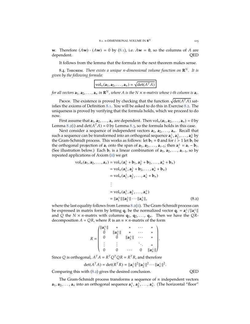
8.1. n-DIMENSIONAL VOLUME IN RN 103
w. Therefore (Aw) · (Aw) 0 by (8.1), i.e. Aw 0, so the columns of A aredependent. QED
It follows from the lemma that the formula in the next theorem makes sense.
8.4. Theorem. There exists a unique n-dimensional volume function on RN . It isgiven by the following formula:
voln (a1, a2, . . . , an) √
det(ATA)
for all vectors a1, a2, . . . , an in RN , where A is the N × n-matrix whose i-th column is ai .
Proof. The existence is proved by checking that the function√
det(ATA) sat-isfies the axioms of Definition 8.1. You will be asked to do this in Exercise 8.2. Theuniqueness is proved by verifying that the formula holds, which we proceed to donow.
First assume that a1, a2, . . . , an are dependent. Then voln (a1 , a2, . . . , an) 0 byLemma 8.2(i) and det(ATA) 0 by Lemma 8.3, so the formula holds in this case.
Next consider a sequence of independent vectors a1, a2, . . . , an . Recall thatsuch a sequence can be transformed into an orthogonal sequence a⊥
1, a⊥
2, . . . , a⊥n by
the Gram-Schmidt process. This works as follows: let b1 0 and for i > 1 let bi bethe orthogonal projection of ai onto the span of a1, a2, . . . , ai−1; then a⊥
i ai − bi .
(See illustration below.) Each bi is a linear combination of a1, a2, . . . , ai−1, so byrepeated applications of Axiom (ii) we get
voln (a1 , a2, . . . , an) voln (a⊥1 + b1 , a⊥2 + b2, . . . , a
⊥n + bn)
voln (a⊥1 , a⊥2 + b2, . . . , a
⊥n + bn )
voln (a⊥1 , a⊥2 , . . . , a
⊥n + bn)
...
voln (a⊥1 , a⊥2 , . . . , a
⊥n )
‖a⊥1 ‖‖a⊥2 ‖ · · · ‖a
⊥n ‖, (8.2)
where the last equality follows from Lemma 8.2(ii). The Gram-Schmidt process canbe expressed in matrix form by letting qi be the normalized vector qi a⊥
i/‖a⊥
i‖
and Q the N × n-matrix with columns q1, q2, . . . , qn . Then we have the QR-decomposition A QR, where R is an n × n-matrix of the form
R
*.......,
‖a⊥1‖ ∗ ∗ · · · ∗
0 ‖a⊥2‖ ∗ · · · ∗
0 0 ‖a⊥3‖ · · · ∗
......
. . . ∗0 0 · · · 0 ‖a⊥n ‖
+///////-
.
Since Q is orthogonal, ATA RT QTQR RT R, and therefore
det(ATA) det(RT R) ‖a⊥1 ‖2‖a⊥2 ‖
2 · · · ‖a⊥n ‖2.Comparing this with (8.2) gives the desired conclusion. QED
The Gram-Schmidt process transforms a sequence of n independent vectorsa1, a2, . . . , an into an orthogonal sequence a⊥
1, a⊥
2, . . . , a⊥n . (The horizontal “floor”
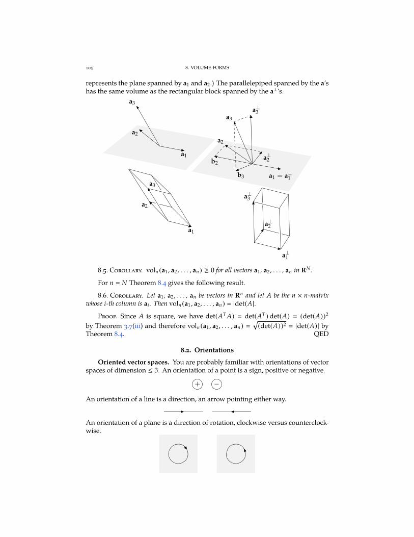
104 8. VOLUME FORMS
represents the plane spanned by a1 and a2.) The parallelepiped spanned by the a’shas the same volume as the rectangular block spanned by the a⊥’s.
a1
a2
a3
a1 = a⊥1
a2
a3
b2
b3
a⊥2
a⊥3
a1
a2
a3
a⊥1
a⊥2
a⊥3
8.5. Corollary. voln (a1, a2, . . . , an) ≥ 0 for all vectors a1, a2, . . . , an in RN .
For n N Theorem 8.4 gives the following result.
8.6. Corollary. Let a1, a2, . . . , an be vectors in Rn and let A be the n × n-matrixwhose i-th column is ai. Then voln (a1 , a2, . . . , an) |det(A|.
Proof. Since A is square, we have det(ATA) det(AT ) det(A) (det(A))2
by Theorem 3.7(iii) and therefore voln (a1, a2, . . . , an)
√
(det(A))2 |det(A) | by
Theorem 8.4. QED
8.2. Orientations
Oriented vector spaces. You are probably familiar with orientations of vectorspaces of dimension ≤ 3. An orientation of a point is a sign, positive or negative.
+ −
An orientation of a line is a direction, an arrow pointing either way.
An orientation of a plane is a direction of rotation, clockwise versus counterclock-wise.
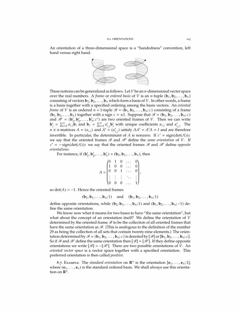
8.2. ORIENTATIONS 105
An orientation of a three-dimensional space is a “handedness” convention, lefthand versus right hand.
These notions can be generalized as follows. Let V be an n-dimensional vector spaceover the real numbers. A frame or ordered basis of V is an n-tuple (b1, b2, . . . , bn)
consisting of vectors b1, b2, . . . , bn which form a basis of V. In other words, a frameis a basis together with a specified ordering among the basis vectors. An orientedframe of V is an ordered n + 1-tuple B (b1, b2, . . . , bn ; ε) consisting of a frame(b1, b2, . . . , bn) together with a sign ε ±1. Suppose that B (b1 , b2, . . . , bn ; ε)
and B′ (b′1, b′
2, . . . , b′n ; ε′) are two oriented frames of V. Then we can write
b′j
∑ni1 ai , jbi and b j
∑ni1 a′
i , jb′
iwith unique coefficients ai , j and a′
i , j. The
n × n-matrices A (ai , j ) and A′ (a′i , j
) satisfy AA′ A′A I and are thereforeinvertible. In particular, the determinant of A is nonzero. If ε′ sign(det(A))εwe say that the oriented frames B and B′ define the same orientation of V. Ifε′ − sign(det(A))ε we say that the oriented frames B and B
′ define oppositeorientations.
For instance, if (b′1, b′
2, . . . , b′n) (b2 , b1, . . . , bn ), then
A
*.......,
0 1 0 . . . 01 0 0 . . . 00 0 1 . . . 0...
......
. . ....
0 0 0 . . . 1
+///////-
,
so det(A) −1. Hence the oriented frames
(b2 , b1, . . . , bn ; 1) and (b1 , b2, . . . , bn ; 1)
define opposite orientations, while (b2, b1, . . . , bn ; 1) and (b1, b2, . . . , bn ;−1) de-fine the same orientation.
We know now what it means for two bases to have “the same orientation”, butwhat about the concept of an orientation itself? We define the orientation of Vdetermined by the oriented frame B to be the collection of all oriented frames thathave the same orientation as B. (This is analogous to the definition of the number29 as being the collection of all sets that contain twenty-nine elements.) The orien-tation determined by B (b1 , b2, . . . , bn ; ε) is denoted by [B] or [b1, b2, . . . , bn ; ε].So if B and B′ define the same orientation then [B] [B′]. If they define oppositeorientations we write [B] −[B′]. There are two possible orientations of V. Anoriented vector space is a vector space together with a specified orientation. Thispreferred orientation is then called positive.
8.7. Example. The standard orientation on Rn is the orientation [e1, . . . , en ; 1],where (e1, . . . , en) is the standard ordered basis. We shall always use this orienta-tion on Rn .
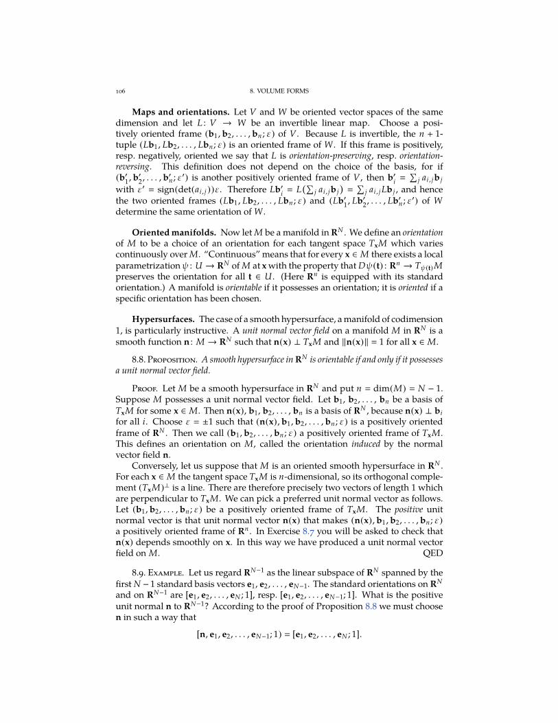
106 8. VOLUME FORMS
Maps and orientations. Let V and W be oriented vector spaces of the samedimension and let L : V → W be an invertible linear map. Choose a posi-tively oriented frame (b1 , b2, . . . , bn ; ε) of V. Because L is invertible, the n + 1-tuple (Lb1 , Lb2, . . . , Lbn ; ε) is an oriented frame of W . If this frame is positively,resp. negatively, oriented we say that L is orientation-preserving, resp. orientation-reversing. This definition does not depend on the choice of the basis, for if(b′
1, b′
2, . . . , b′n ; ε′) is another positively oriented frame of V, then b′
i
∑
j ai , jb j
with ε′ sign(det(ai , j ))ε. Therefore Lb′i L
(∑
j ai , jb j)
∑
j ai , j Lb j , and hencethe two oriented frames (Lb1 , Lb2, . . . , Lbn ; ε) and (Lb′
1, Lb′
2, . . . , Lb′n ; ε′) of W
determine the same orientation of W .
Oriented manifolds. Now let M be a manifold in RN . We define an orientationof M to be a choice of an orientation for each tangent space TxM which variescontinuously over M. “Continuous” means that for every x ∈ M there exists a localparametrizationψ : U → RN of M at x with the property that Dψ(t) : Rn → Tψ(t)Mpreserves the orientation for all t ∈ U . (Here Rn is equipped with its standardorientation.) A manifold is orientable if it possesses an orientation; it is oriented if aspecific orientation has been chosen.
Hypersurfaces. The case of a smooth hypersurface, a manifold of codimension1, is particularly instructive. A unit normal vector field on a manifold M in RN is asmooth function n : M → RN such that n(x) ⊥ TxM and ‖n(x)‖ 1 for all x ∈ M.
8.8. Proposition. A smooth hypersurface in RN is orientable if and only if it possessesa unit normal vector field.
Proof. Let M be a smooth hypersurface in RN and put n dim(M) N − 1.Suppose M possesses a unit normal vector field. Let b1, b2, . . . , bn be a basis ofTxM for some x ∈ M. Then n(x), b1, b2, . . . , bn is a basis of RN , because n(x) ⊥ bi
for all i. Choose ε ±1 such that (n(x), b1, b2, . . . , bn ; ε) is a positively orientedframe of RN . Then we call (b1, b2, . . . , bn ; ε) a positively oriented frame of TxM.This defines an orientation on M, called the orientation induced by the normalvector field n.
Conversely, let us suppose that M is an oriented smooth hypersurface in RN .For each x ∈ M the tangent space TxM is n-dimensional, so its orthogonal comple-ment (TxM)⊥ is a line. There are therefore precisely two vectors of length 1 whichare perpendicular to TxM. We can pick a preferred unit normal vector as follows.Let (b1, b2, . . . , bn ; ε) be a positively oriented frame of TxM. The positive unitnormal vector is that unit normal vector n(x) that makes (n(x), b1 , b2, . . . , bn ; ε)
a positively oriented frame of Rn . In Exercise 8.7 you will be asked to check thatn(x) depends smoothly on x. In this way we have produced a unit normal vectorfield on M. QED
8.9. Example. Let us regard RN−1 as the linear subspace of RN spanned by thefirst N − 1 standard basis vectors e1, e2, . . . , eN−1. The standard orientations on RN
and on RN−1 are [e1, e2, . . . , eN ; 1], resp. [e1, e2, . . . , eN−1; 1]. What is the positiveunit normal n to RN−1? According to the proof of Proposition 8.8 we must choosen in such a way that
[n, e1, e2, . . . , eN−1; 1) [e1, e2, . . . , eN ; 1].
8.3. VOLUME FORMS 107
The only two possibilities are n ρeN with ρ ±1. By parts (i) and (iv) of Exercise8.5 we have
[n, e1, e2, . . . , eN−1; 1] (−1)N+1[e1, e2, . . . , eN−1, n; 1]
(−1)N+1[e1, e2, . . . , eN−1, ρeN ; 1] (−1)N+1ρ[e1, e2, . . . , eN−1, eN ; 1],
so we want (−1)N+1ρ 1. We conclude that the positive unit normal to RN−1 inRN is (−1)N+1eN .
The positive unit normal on an oriented smooth hypersurface M in RN can beregarded as a map n from M into the unit sphere SN−1, which is often called theGauss map of M. The unit normal enables one to distinguish between two sides ofM: the direction of n is “out” or “up”; the opposite direction is “in” or “down”.For this reason orientable hypersurfaces are often called two-sided, whereas thenonorientable ones are called one-sided. Let us show that a hypersurface given bya single equation is always orientable.
8.10. Proposition. Let U be open in RN and let φ : U → R be a smooth function.Let c be a regular value of φ. Then the smooth hypersurface φ−1(c) has a unit normalvector field given by n(x) grad(φ)(x)/‖grad(φ)(x)‖ and is therefore orientable.
Proof. The regular value theorem tells us that M φ−1(c) is a smooth hyper-surface in RN (if nonempty), and also that TxM ker(Dφ(x)) grad(φ)(x)⊥. Thefunction n(x) grad(φ)(x)/‖grad(φ)(x)‖ therefore defines a unit normal vectorfield on M. Appealing to Proposition 8.8 we conclude that M is orientable. QED
8.11. Example. Taking φ(x) ‖x‖2 and c r2 we obtain that the sphere ofradius r about the origin is orientable. The unit normal is
n(x) grad(φ)(x)/‖grad(φ)(x)‖ x/‖x‖.
8.3. Volume forms
Now let M be an oriented n-manifold in RN . Choose an atlas of M consisting oflocal parametrizations ψi : Ui → RN with the property that Dψi (t) : Rn → TxM isorientation-preserving for all t ∈ Ui. The volume form µM , also denoted by µ, is then-form on M whose local representative relative to the embedding ψi is definedby
µi ψ∗i (µ)
√
det(Dψi (t)T Dψi (t)) dt1 dt2 · · · dtn .
Theorem 8.4 tells us that the square-root factor measures the volume of the n-dimensional parallelepiped in the tangent space TxM spanned by the columns ofDψi (t), the Jacobi matrix of ψi at t. Hence you should think of µ as measuring thevolume of infinitesimal parallelepipeds inside M.
8.12. Theorem. For any oriented n-manifold M in RN the volume form µM is awell-defined n-form.
Proof. To show that µ is well-defined we need to check that its local represen-tatives satisfy the transformation law (7.1). So let us put φ ψ−1
iψ j and substitute
t φ(u) into µi . Since each of the embeddings ψi is orientation-preserving, wehave det(Dφ) > 0. Hence by Theorem 3.14 we have
φ∗(dt1 dt2 · · · dtn) det(Dφ(u) du1 du2 · · · dun |det(Dφ(u)) | du1 du2 · · · dun .
108 8. VOLUME FORMS
Therefore
φ∗(µi )
√
det(
Dψi (φ(u))T Dψi (φ(u))) |det(Dφ(u)) | du1 du2 · · · dun
√
det(Dφ(u))T det(
Dψi (φ(u))T Dψi (φ(u)))
det(Dφ(u)) du1 du2 · · · dun
√
det(
(Dψi (φ(u))Dφ(u))T Dψi (φ(u))Dφ(u))
du1 du2 · · · dun
√
det((Dψ j (u))T Dψ j (u)) du1 du2 · · · dun µ j ,
where in the second to last identity we applied the chain rule. QED
For n 1 the volume form is usually called the element of arc length, for n 2,the element of surface area, and for n 3, the volume element. Traditionally these aredenoted by ds, dA, and dV, respectively. Don’t be misled by these old-fashionednotations: volume forms are seldom exact! Another thing to remember is that thevolume form µM depends on the embedding of M into RN . It changes if we dilateor shrink or otherwise deform M.
8.13. Example. Let U be an open subset of Rn . Recall from Example 6.4 that Uis a manifold covered by a single embedding, namely the identity map ψ : U → U ,ψ(x) x. Then det(DψT Dψ) 1, so the volume form on U is simply dt1 dt2 · · · dtn ,the ordinary volume form on Rn .
8.14. Example. Let I be an interval in the real line and f : I → R a smoothfunction. Let M ⊆ R2 be the graph of f . By Example 6.6 M is a 1-manifold in R2.Indeed, M is the image of the embedding ψ : I → R2 given by ψ(t) (t , f (t)). Letus give M the orientation induced by the embedding ψ, i.e. “from left to right”.What is the element of arc length of M? Let us compute the pullback ψ∗(µ), a1-form on I. We have
Dψ(t)
(
1f ′(t)
)
, Dψ(t)T Dψ(t) (
1 f ′(t))(
1f ′(t)
)
1 + f ′(t)2 ,
so ψ∗(µ) √
det(Dψ(t)T Dψ(t)) dt √
1 + f ′(t)2 dt.
The next result can be regarded as an alternative definition of µM . It is perhapsmore intuitive, but it requires familiarity with Section 7.2.
8.15. Proposition. Let M be an oriented n-manifold in RN . Let x ∈ M and v1,v2, . . . , vn ∈ TxM. Then the volume form of M is given by
µM,x(v1 , v2, . . . , vn )
voln (v1 , v2 , . . . , vn ) if (v1 , v2 , . . . , vn ; 1) is a positively oriented frame,
− voln (v1 , v2 , . . . , vn ) if (v1 , v2 , . . . , vn ; 1) is a negatively oriented frame,
0 if v1, v2 , . . . , vn are linearly dependent,
i.e. µM,x(v1 , v2, . . . , vn ) is the oriented volume of the n-dimensional parallelepiped in TxMspanned by v1, v2 , . . . , vn .
Proof. For each x in M and n-tuple of tangent vectors v1, v2, . . . , vn at x letωx(v1 , v2, . . . , vn ) be the oriented volume of the block spanned by these n vectors.This defines an n-form ω on M and we must show that ω µM . Let U be an opensubset of Rn and ψ : U → RN an orientation-preserving local parametrization of
8.3. VOLUME FORMS 109
M. Choose t ∈ U satisfying ψ(t) x. Let us calculate the n-form ψ∗(ω) on U . Wehave ψ∗(ω) g dt1 dt2 · · · dtn for some function g. By Lemma 7.12 this function isgiven by
g(t) ψ∗(ωx)(e1, e2, . . . , en) ωx(Dψ(t)e1,Dψ(t)e2, . . . ,Dψ(t)en),
where in the second equality we used the definition of pullback. Then thetuple (Dψ(t)e1,Dψ(t)e2, . . . ,Dψ(t)en ; 1) is a positively oriented frame of TxMand, moreover, are the columns of the matrix Dψ(t), so by Theorem 8.4 theyspan a positive volume of magnitude
√
det(Dψ(t)T Dψ(t)). This shows thatg
√
det(DψT Dψ) and therefore
ψ∗(ω)
√
det(DψT Dψ) dt1 dt2 · · · dtn .
Thusψ∗(ω) is equal to the local representative of µM with respect to the embeddingψ. Since this holds for all embeddings ψ, we have ω µM . QED
Volume form of a hypersurface. Recall the vector-valued forms
dx
*..,
dx1
...dxN
+//-
and ∗dx
*..,
∗dx1
...∗dxN
+//-
on RN , which were introduced in Section 2.5. We will use these forms to give aconvenient expression for the volume form on a hypersurface. Let M be an orientedhypersurface in RN . Let n be the positive unit normal vector field on M and let F
be any vector field on M, i.e. a smooth map F : M → RN . Then the inner productF · n is a function defined on M. It measures the component of F orthogonal to M.The product (F · n)µM is an n-form on M, where n dim(M) N − 1. On theother hand we have the n-form ∗(F · dx) F · ∗dx.
8.16. Theorem. On the hypersurface M we have
F · ∗dx (F · n)µM .
First proof. This proof is short but requires familiarity with the material inSection 7.2. Let x ∈ M. Let us make an orthogonal change of coordinates in RN
in such a way that (e1, e2 . . . , eN−1; 1) is a positively oriented frame of TxM. Then,according to Example 8.9, the positive unit normal at x is given by n(x) (−1)N+1eN
and the volume form satisfies µM,x(e1 , . . . , eN−1) 1. Writing F
∑Ni1 Fiei, we
have F(x) · n(x) (−1)N+1FN (x). On the other hand
F · ∗dx
∑
i
(−1)i+1Fi dx1 · · · dx i · · · dxN ,
and therefore (F · ∗dx)(e1, . . . , eN−1) (−1)N+1FN . This proves that
(F · ∗dx)x(e1 , . . . , eN−1) (F(x) · n(x))µM (e1, . . . , eN−1),
which implies (F ·∗dx)x (F(x) ·n(x))µM. Since this equality holds for every x ∈ M,we find F · ∗dx (F · n)µM . QED
Second proof. Choose a local parametrizationψ : U → RN of M at x. Let t ∈ Ube the point satisfying ψ(t) x. As a preliminary step in the proof we are goingto replace the embedding ψ with a new one enjoying a particularly nice property.
110 8. VOLUME FORMS
Let us change the coordinates on RN in such a way that (e1, e2 . . . , eN−1; 1) is apositively oriented frame of TxM. Then at x the positive unit normal is given byn(x) (−1)N+1eN . Since the columns of the Jacobi matrix Dψ(t) are independent,there exist unique vectors a1, a2, . . . , aN−1 in RN−1 such that Dψ(t)ai ei for i 1,2, . . . , N − 1. These vectors ai are independent, because the ei are independent.Therefore the (N − 1) × (N − 1)-matrix A with i-th column vector equal to ai isinvertible. Put U A−1(U), t A−1t and ψ ψ A. Then U is open in RN−1,ψ(t) x, ψ : U → RN is an embedding with ψ(U) ψ(U), and
Dψ(t) Dψ(t) DA(t) Dψ(t) A
by the chain rule. Therefore the i-th column vector of Dψ(t) is
Dψ(t)ei Dψ(t)Aei Dψ(t)ai ei (8.3)
for i 1, 2, . . . , N −1. (On the left ei denotes the i-th standard basis vector in RN−1,on the right it denotes the i-th standard basis vector in RN .) In other words, theJacobi matrix of ψ at t is the (N − 1) × N-matrix
Dψ(t)
(
IN−1
0
)
,
where IN−1 is the (N − 1) × (N − 1) identity matrix and 0 denotes a row consistingof N − 1 zeros.
Let us now calculate ψ∗(
(F · n)µM)
and ψ∗(F · ∗dx) at the point t. WritingF · n
∑Ni1 Fini and using the definition of µM we get
ψ∗(
(F · n)µM)
( N∑
i1
ψ∗(Fi ni )
)√
det(DψT Dψ) dt1 dt2 · · · dtN−1.
From formula (8.3) we have det(Dψ(t)T Dψ(t)) 1. So evaluating this expressionat the point t and using n(x) (−1)N+1eN we get
(
ψ∗(F · n)µM)
t (−1)N+1FN (x) dt1 dt2 · · · dtN−1.
From F · ∗dx
∑Ni1(−1)i+1Fi dx1 dx2 · · · dx i · · · dxN we get
ψ∗(F · ∗dx)
N∑
i1
(−1)i+1ψ∗(Fi ) dψ1 dψ2 · · · dψi · · · dψN .
From formula (8.3) we see ∂ψi (t)/∂t j δi , j for 1 ≤ i, j ≤ N − 1 and ∂ψN (t)/∂t j 0for 1 ≤ j ≤ N − 1. Therefore
(
ψ∗(F · ∗dx))
t (−1)N+1FN (x) dt1 dt2 · · · dtN−1.
We conclude that(
ψ∗(F · n)µM)
t (
ψ∗(F · ∗dx))
t, in other words(
(F · n)µM)
x
(F · ∗dx)x. Since this holds for all x ∈ M we have F · ∗dx (F · n)µM . QED
This theorem gives insight into the physical interpretation of N − 1-forms onRN . Think of the vector field F as representing the flow of a fluid or gas. Thedirection of the vector F indicates the direction of the flow and its magnitudemeasures the strength of the flow. Then Theorem 8.16 says that the N − 1-formF · ∗dx measures, for any unit vector n in RN , the amount of fluid per unit of timepassing through a hyperplane of unit volume perpendicular to n. We call F · ∗dxthe flux of the vector field F.
EXERCISES 111
Another application of the theorem are the following formulas involving thevolume form on a hypersurface. The formulas provide a heuristic interpretationof the vector-valued form ∗dx: if n is a unit vector in RN , then the scalar-valuedN − 1-form n · ∗dx measures the volume of an infinitesimal N − 1-dimensionalparallelepiped perpendicular to n.
8.17. Corollary. Let n be the unit normal vector field and µM the volume form of theoriented hypersurface M. Then
µM n · ∗dx and ∗dx nµM .
Proof. Set F n in Theorem 8.16. Then F · n 1, because ‖n‖ 1, andhence µM n · ∗dx. Now take F to be any vector field that is tangent to M.Then F · n 0, because n is normal to M, so F · ∗dx 0. It follows that on thehypersurface M the Rn-valued n − 1-form ∗dx is equal to the product of n and ascalar n − 1-form ν: ∗dx nν. Taking the dot product of both sides with n weobtain ν n · nν n · ∗dx µM , i.e. ∗dx nµM . QED
8.18. Example. Suppose the hypersurface M is given by an equation φ(x) c,where c is a regular value of a function φ : U → R, with U open in Rn . Then byProposition 8.10 M has a unit normal n grad(φ)/‖grad(φ)‖. The volume form istherefore µ ‖grad(φ)‖−1 grad(φ) · ∗dx. In particular, if M is the sphere of radiusR about the origin in Rn , then n(x) x/R, so µM R−1x · ∗dx.
Exercises
8.1. Let a and b be vectors in RN .
(i) Deduce from Theorem 8.4 that the area of the parallelogram spanned by a and bis given by ‖a‖ ‖b‖ sinφ, where φ is the angle between a and b (which is takento lie between 0 and π).
(ii) Show that for N 3 we have ‖a‖ ‖b‖ sinφ ‖a×b‖. (Consider det(a, b, a×b).)
8.2. Check that the function voln (a1 , a2 , . . . , an )
√
det(AT A) satisfies the axioms ofDefinition 8.1.
8.3. Let u1, u2 , . . . , uk and v1, v2 , . . . , vl be vectors in RN satisfying ui · v j 0 for i 1,
2, . . . , k and j 1, 2, . . . , l. (“The u’s are perpendicular to the v’s.”) Prove that
volk+l (u1 , u2 , . . . , uk , v1 , v2 , . . . , vl ) volk (u1 ,u2 , . . . , uk ) voll (v1 , v2 , . . . , vl ).
8.4. Let a1, a2 , . . . , an be real numbers, let c
√
1 +∑n
i1a2
iand let
u1
*.......,
10...0a1
+///////-
, u2
*.......,
01...0a2
+///////-
, . . . , un
*.......,
00...1
an
+///////-
, un+1
1
c
*.......,
−a1
−a2...−an
1
+///////-
be vectors in Rn+1.
(i) Deduce from Exercise 8.3 that
voln (u1 ,u2 , . . . , un ) voln+1(u1 , u2 , . . . , un ,un+1).
112 8. VOLUME FORMS
(ii) Prove that
1 + a21
a1a2 a1a3 . . . a1an
a2a1 1 + a22
a2a3 . . . a2an
a3a1 a3a2 1 + a23
. . . a3an
......
.... . .
...an a1 an a2 an a3 . . . 1 + a2
n
1 +
n∑
i1
a2i .
8.5. Let V be an n-dimensional vector space with basis b1, b2 , . . . , bn . Let ε ±1.Prove the following identities concerning orientations of V .
(i) [b1 , . . . , cbi , . . . , bn ; ε] sign(c)[b1 , . . . , bi , . . . , bn ; ε] for all nonzero scalars c.(ii) [b1 , b2 , . . . , bn ; ε] ε[b1 ,b2 , . . . , bn ; 1].
(iii) [b1 , b2 , . . . , bn ;−ε] −[b1 , b2 , . . . , bn ; ε].(iv)
[
bσ(1) , bσ(2) , . . . , bσ(n) ; ε]
sign(σ)[b1 , b2 , . . . , bn ; ε] for all permutations σ inSn .
8.6. A frame (b1 , b2 , . . . , bn ) of Rn is orthonormal if the vectors b1, b2 , . . . , bn forman orthonormal basis of Rn . Denote the set of orthonormal frames by Fn and the set ofpositively oriented orthonormal frames by F+
n .
(i) Explain how to identify Fn with the orthogonal group O(n) and F+n with the
special orthogonal group SO(n). Conclude that Fn and F+n are manifolds of
dimension 12 n(n − 1). (Use Theorem 6.18).
(ii) Explain how to identify F+3
with the configuration space M0 discussed in Exam-
ple 1.7 and conclude that M0 is a three-dimensional projective space. (See thediscussion following Theorem 6.18).
8.7. Show that the unit normal vector field n : M → RN defined in the proof of Proposi-tion 8.8 is smooth. (Compute n in terms of an orientation-preserving local parametrizationψ of M.)
8.8. Let U be open in Rn and let f : U → R be a smooth function. Let ψ : U → Rn+1 bethe embedding ψ(x) (x, f (x)) and let M ψ(U), the graph of f . We define an orientationon M by requiringψ to be orientation-preserving. Deduce from Exercise 8.4 that the volume
form of M is given by ψ∗(µM )
√
1 + ‖grad f (x)‖2 dx1 dx2 · · · dxn .
8.9. Let M graph( f ) be the oriented hypersurface of Exercise 8.8.
(i) Show that the positive unit normal vector field on M is given by
n
(−1)n+1
√
1 + ‖grad( f )(x)‖2
*.......,
∂ f /∂x1
∂ f /∂x2...
∂ f /∂xn
−1
+///////-
.
(ii) Derive the formula ψ∗ (µM )
√
1 + ‖grad f (x)‖2 dx1 dx2 · · · dxn of Exercise 8.8
from Corollary 8.17 by substituting xn+1 f (x1 , x2 , . . . , xn ). (You must replaceN with n + 1 in Corollary 8.17.)
8.10. Let ψ : U → RN be an embedding of an open subset U of Rn into RN . Let M bethe image of ψ and let µ be the volume form of M. Now let R be a nonzero number, let ψR
be the embedding ψR (t) Rψ(t), let MR be the image of ψR , and let µR be the volume form
of MR. Show that ψ∗R
(µR ) Rnψ∗(µ). (Use ψ∗ (µ)
√
det(Dψi (t)T Dψi (t)) dt1 dt2 · · · dtn .)
CHAPTER 9
Integration and Stokes’ theorem for manifolds
In this chapter we will see how to integrate an n-form over an oriented n-manifold. In particular, by integrating the volume form we find the volume of themanifold. We will also discuss a version of Stokes’ theorem for manifolds. Thisrequires the slightly more general notion of a manifold with boundary.
9.1. Manifolds with boundary
The notion of a spherical earth developed in classical Greece around the time ofPlato and Aristotle. Older cultures (and also Western culture until the rediscoveryof Greek astronomy in the late Middle Ages) visualized the earth as a flat discsurrounded by an ocean or a void. A closed disc is not a manifold, because noneighbourhood of a point on the edge is the image of an open subset of R2 underan embedding. Rather, it is a manifold with boundary, a notion which is definedas follows. The n-dimensional half-space is
Hn x ∈ Rn | xn ≥ 0 .
The boundary of Hn is ∂Hn x ∈ Rn | xn 0 and its interior is int(Hn) x ∈
Rn | xn > 0 .
9.1. Definition. An n-dimensional manifold with boundary (or n-manifold withboundary) in RN is a subset M of RN such that for each x ∈ M there exist
• an open subset V ⊆ RN containing x,• an open subset U ⊆ Rn ,• and an embedding ψ : U → RN satisfying ψ(U ∩Hn ) M ∩ V.
You should compare this definition carefully with Definition 6.3 of a manifold. Ifx ψ(t) with t ∈ ∂Hn , then x is a boundary point of M. The boundary of M is theset of all boundary points and is denoted by ∂M. Its complement M \ ∂M is theinterior of M and is denoted by int(M).
Definition 9.1 does not rule out the possibility that the boundary of an n-manifold with boundary might be empty! If the boundary of M is empty, then Mis a manifold in the sense of Definition 6.3. If the boundary ∂M is nonempty, then∂M is an n − 1-dimensional manifold. The interior int(M) is an n-manifold.
The most obvious example of an n-manifold with boundary is the half-spaceHn itself. Its boundary is the hyperplane ∂Hn , which is a copy of Rn−1, and itsinterior is the open half-space x ∈ Rn | xn > 0 . Here is a more interesting typeof example, which generalizes the graph of a function.
9.2. Example. Let U′ be an open subset of Rn−1 and let f : U′→ R be a smoothfunction. Put U U′ × R and write elements of U as
(xy)
with x in U′ and y in R.
113
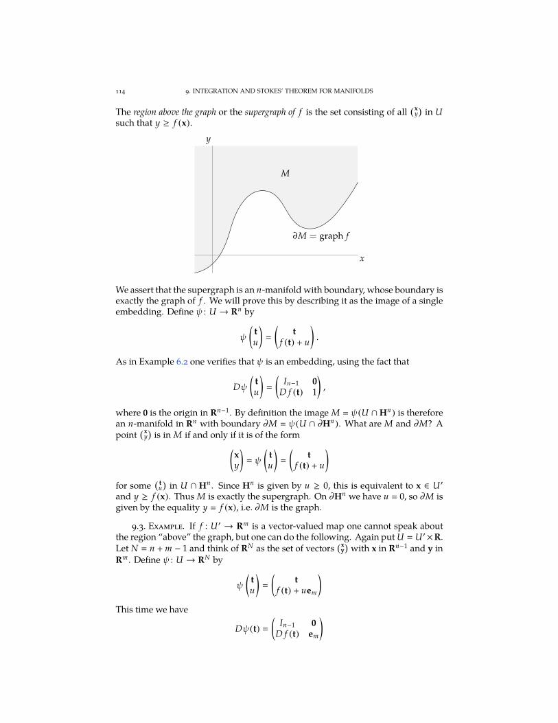
114 9. INTEGRATION AND STOKES’ THEOREM FOR MANIFOLDS
The region above the graph or the supergraph of f is the set consisting of all(x
y)
in Usuch that y ≥ f (x).
∂M = graph f
M
x
y
We assert that the supergraph is an n-manifold with boundary, whose boundary isexactly the graph of f . We will prove this by describing it as the image of a singleembedding. Define ψ : U → Rn by
ψ
(
tu
)
(
tf (t) + u
)
.
As in Example 6.2 one verifies that ψ is an embedding, using the fact that
Dψ
(
tu
)
(
In−1 0D f (t) 1
)
,
where 0 is the origin in Rn−1. By definition the image M ψ(U ∩Hn ) is thereforean n-manifold in Rn with boundary ∂M ψ(U ∩ ∂Hn ). What are M and ∂M? Apoint
(xy)
is in M if and only if it is of the form(
xy
)
ψ
(
tu
)
(
tf (t) + u
)
for some( t
u)
in U ∩ Hn . Since Hn is given by u ≥ 0, this is equivalent to x ∈ U′
and y ≥ f (x). Thus M is exactly the supergraph. On ∂Hn we have u 0, so ∂M isgiven by the equality y f (x), i.e. ∂M is the graph.
9.3. Example. If f : U′ → Rm is a vector-valued map one cannot speak aboutthe region “above” the graph, but one can do the following. Again put U U′×R.Let N n + m − 1 and think of RN as the set of vectors
(xy)
with x in Rn−1 and y inRm . Define ψ : U → RN by
ψ
(
tu
)
(
tf (t) + uem
)
This time we have
Dψ(t)
(
In−1 0D f (t) em
)
9.1. MANIFOLDS WITH BOUNDARY 115
and again ψ is an embedding. Therefore M ψ(U ∩Hn ) is an n-manifold in RN
with boundary ∂M ψ(U ∩ ∂Hn ). This time M is the set of points(xy)
of the form
(
xy
)
(
tf (t) + uem
)
with t ∈ U′ and u ≥ 0. Hence M is the set of points(xy)
where x is in U′ and wherey satisfies m − 1 equalities and one inequality:
y1 f1(x), y2 f2(x), . . . , ym−1 fm−1(x), ym ≥ fm (x).
Again ∂M is given by y f (x), so ∂M is the graph of f .
Here is an extension of the regular value theorem, Theorem 6.12, to manifoldswith boundary.
9.4. Theorem (regular value theorem for manifolds with boundary). Let U beopen in RN and let φ : U → Rm be a smooth map. Let M be the set of x in RN satisfying
φ1(x) c1 , φ2(x) c2 , . . . , φm−1(x) cm−1 , φm (x) ≥ cm .
Suppose that c (c1 , c2 , . . . , cm ) is a regular value of φ and that M is nonempty. Then
M is a manifold in RN of codimension m − 1 and with boundary ∂M φ−1(c).
We will not spell out the proof, which is similar to that of Theorem 6.12. Thestatement remains true if we replace “≥” with “≤”, as one sees by replacing φwith−φ.
9.5. Example. Let U Rn , m 1 and φ(x) ‖x‖2. The set given by theinequality φ(x) ≤ 1 is then the closed unit ball x ∈ Rn | ‖x‖ ≤ 1 . Sincegrad(φ)(x) 2x, any nonzero value is a regular value of φ. Hence the ball is ann-manifold in Rn , whose boundary is φ−1(1), the unit sphere Sn−1.
If more than one inequality is involved, singularities often arise. A simpleexample is the closed quadrant in R2 given by the pair of inequalities x ≥ 0 andy ≥ 0. This is not a manifold with boundary because its edge has a sharp angle atthe origin. Similarly, a closed square is not a manifold with boundary.
However, one can show that a set given by a pair of inequalities of the forma ≤ f (x) ≤ b, where a and b are both regular values of a function f , is a manifoldwith boundary. For instance, the spherical shell
x ∈ Rn | R1 ≤ ‖x‖ ≤ R2
is an n-manifold whose boundary is a union of two concentric spheres.
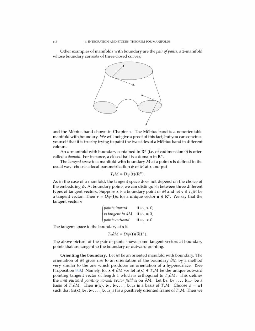
116 9. INTEGRATION AND STOKES’ THEOREM FOR MANIFOLDS
Other examples of manifolds with boundary are the pair of pants, a 2-manifoldwhose boundary consists of three closed curves,
and the Möbius band shown in Chapter 1. The Möbius band is a nonorientablemanifold with boundary. We will not give a proof of this fact, but you can convinceyourself that it is true by trying to paint the two sides of a Möbius band in differentcolours.
An n-manifold with boundary contained in Rn (i.e. of codimension 0) is oftencalled a domain. For instance, a closed ball is a domain in Rn .
The tangent space to a manifold with boundary M at a point x is defined in theusual way: choose a local parametrization ψ of M at x and put
TxM Dψ(t)(Rn).
As in the case of a manifold, the tangent space does not depend on the choice ofthe embedding ψ. At boundary points we can distinguish between three differenttypes of tangent vectors. Suppose x is a boundary point of M and let v ∈ TxM bea tangent vector. Then v Dψ(t)u for a unique vector u ∈ Rn . We say that thetangent vector v
points inward if un > 0,
is tangent to ∂M if un 0,
points outward if un < 0.
The tangent space to the boundary at x is
Tx∂M Dψ(t)(∂Hn ).
The above picture of the pair of pants shows some tangent vectors at boundarypoints that are tangent to the boundary or outward pointing.
Orienting the boundary. Let M be an oriented manifold with boundary. Theorientation of M gives rise to an orientation of the boundary ∂M by a methodvery similar to the one which produces an orientation of a hypersurface. (SeeProposition 8.8.) Namely, for x ∈ ∂M we let n(x) ∈ TxM be the unique outwardpointing tangent vector of length 1 which is orthogonal to Tx∂M. This definesthe unit outward pointing normal vector field n on ∂M. Let b1, b2, . . . , bn−1 be abasis of Tx∂M. Then n(x), b1, b2, . . . , bn−1 is a basis of TxM. Choose ε ±1such that (n(x), b1 , b2, . . . , bn−1; ε) is a positively oriented frame of TxM. Then we
9.2. INTEGRATION OVER ORIENTABLE MANIFOLDS 117
define (b1, b2, . . . , bn−1; ε) to be a positively oriented frame of Tx∂M. The resultingorientation of ∂M is called the induced orientation.
9.6. Example. Consider the upper half-space Hn with its standard orientation[e1, . . . , en ; 1]. At each point of ∂Hn the outward pointing normal is −en . Since
[−en , e1, e2, . . . , en−1; 1] −[en , e1, e2, . . . , en−1; 1]
−(−1)n−1[e1, e2, . . . , en−1, en ; 1] [e1, e2, . . . , en−1, en ; (−1)n],
the induced orientation on ∂Hn is [e1, e2, . . . , en−1; (−1)n].
You may wonder why we didn’t get rid of the (−1)n by adopting a differentconvention for the orientation of the boundary. The justification for our conventionis that it avoids the need for sign corrections in the statement of Stokes’ theorem,Theorem 9.9.
9.2. Integration over orientable manifolds
As we saw in Chapter 5, a form of degree n can be integrated over a chainof dimension n. The integral does not change if we reparametrize the chain inan orientation-preserving manner. This suggests the possibility of integrating ann-form over an oriented n-manifold. One might try to do this by breaking up themanifold into n-chains and then integrating over each of the chains, but that turnsout to be not so easy. Instead we shall employ the simpler method of breaking thedifferential form into small pieces and then integrating each of the pieces.
In the remainder of this section M ⊆ RN denotes an n-manifold with boundaryand α denotes a differential form on M.
Support. The support of α is defined as the set of all points x in M with theproperty that for every open ball B around x there is a y ∈ B ∩M such that αy , 0.The support of α is denoted by supp(α). If αx is nonzero, then x is in the supportof α (because we can take y x for all B). But for x to be in the support it is notnecessary for αx to be nonzero; we only need to be able to find points arbitrarilyclose to x where α is nonzero. In other words, x is not in the support if and only ifthere exists a ball B around x such that αy 0 for all y ∈ B ∩M.
9.7. Example. Let M R and αi fi dx, where fi is one of the following smoothfunctions.
(i) f1(x) sin x. This function has infinitely many zeroes, but they are allisolated: sinπk 0, but sin y , 0 for y close to but distinct from πk.Thus supp(α1) R.
(ii) f2 is a nonzero polynomial function. Again f2 has isolated zeroes, sosupp(α2) R.
(iii) f3(x) exp(−1/x) for x > 0 and f3(x) 0 for x ≤ 0. (This function issimilar to the function of Exercise B.3.) We have f3(x) > 0 for all x > 0.It follows that x ∈ supp(α3) for all x ≥ 0. On the other hand, negative xare not in the support, so supp(α3) [0,∞).
(iv) f4(x) f3(x − a) f3(b − x), where a < b are constants. We have f4(x) > 0for a < x < b and f4(x) 0 for x < a and x > b. Hence supp(α4) [a, b].
9.8. Example. The volume form µ of M is nowhere 0, so supp(µ) M.
118 9. INTEGRATION AND STOKES’ THEOREM FOR MANIFOLDS
Partitions of unity. Chopping differential forms into “little pieces” requires adevice known as a partition of unity. Let ψi : Ui → RN be an atlas of M, where iruns over an indexing set I . A partition of unity subordinate to the atlas is a collectionof smooth functions λi : M → R with the following properties:
(i) λi ≥ 0 for all i;(ii) supp(λi ) is contained in ψi (Ui ) for all i;
(iii) for every x ∈ M there exists a ball B around x with the property thatsupp(λi ) ∩ B is empty for all but finitely many i ∈ I ;
(iv)∑
i∈I λi 1.
Condition (iv) says that the functions λi add up to the constant function 1; it is inthis sense that they “partition” the “unit” function. Together with the positivitycondition (i) this implies that every λi takes values between 0 an 1. Condition(ii) expresses that λi is “small” in another sense as well: for every point x of Mwhich is not contained in the coordinate patch ψi (Ui) the function λi vanishesidentically in a neighbourhood of x. Condition (iii) is imposed to ensure that evenif the indexing set I is infinite the sum in condition (iv) is finite at every point andis a well-defined smooth function.
It is a very useful technical fact that partitions of unity exist subordinate to anyatlas of M. See Chapter 3 of the book [Spi71] for a proof, or see Exercise 9.3 for aspecial case.
Defining the integral. From now on we assume that M is oriented and that αis of degree n dim(M). Moreover, we assume that the support of α is a compactset. (A subset of RN is called compact if it is closed and bounded; see Appendix A.2.The compactness assumption is made to ensure that the integral of α is a properintegral and therefore converges. For instance, if we let M R and αi one of the1-forms of Example 9.7, then only α4 has a well-defined integral over M. Also notethat the support of α is certainly compact if the manifold M itself is compact.)
Step 1. Assume there exists an orientation-preserving local parametrizationψ : U → RN of M with the property that the support of α is contained inψ(U∩Hn).Then we define the integral of α over M by∫
M
α
∫U∩Hn
ψ∗(α).
The right-hand side is well-defined because the integrand is of the form ψ∗(α)
g dt1 dt2 · · · dtn , where g is a smooth function on U ∩Hn which vanishes outsidea compact subset. Moreover, the integral does not depend on the choice of ψ: ifψ′ : U′ → RN is another orientation-preserving local parametrization of M suchthat supp(α) is contained in ψ′(U′ ∩ Hn), then, letting ζ ψ−1 ψ′, we haveψ ζ ψ′, so∫
U′∩Hn(ψ′)∗α
∫U′∩Hn
(ψ ζ)∗(α)
∫U′∩Hn
ζ∗(ψ∗(α))
∫U∩Hn
ψ∗(α),
where the last step uses Theorem 5.1 and the fact that ζ preserves the orientation.Step 2. In the general case we choose an atlas of M consisting of orientation-
preserving local parametrizationsψi : Ui → RN , and we choose a partition of unitysubordinate to this atlas consisting of functions λi : M → R. Let αi λiα. Then αi
is an n-form with support contained in ψi (Ui ∩Hn ), so its integral is well-defined
9.2. INTEGRATION OVER ORIENTABLE MANIFOLDS 119
by step 1. Moreover,∑
i∈I αi ∑
i∈I λiα (∑
i∈I λi )α α. We now define theintegral of α by ∫
M
α
∑
i∈I
∫M
αi
∑
i∈I
∫Ui∩Hn
ψ∗i (αi ). (9.1)
The most important property of the integral is the following version of Stokes’theorem, which can be viewed as a parametrization-independent version of Theo-rem 5.11.
9.9. Theorem (Stokes’ theorem for manifolds). Let α be an n − 1-form withcompact support on an oriented n-manifold with boundary M. Give the boundary ∂M theinduced orientation. Then ∫
M
dα
∫∂M
α.
Proof. Step 1. Suppose M Hn . Then we can write
α
n∑
i1
gi dt1 dt2 · · · dt i · · · dtn
for certain smooth functions gi defined on Hn . We have
dα
n∑
i1
(−1)i+1 ∂gi
∂tidt1 dt2 · · · dtn .
The support of α is a compact subset of Hn and so is enclosed in a box of the shape
[a1, b1] × [a2 , b2] × · · · × [an−1, bn−1] × [0, c]. (9.2)
Therefore ∫Hn
dα
n∑
i1
(−1)i+1
∫ c
0
∫ bn−1
an−1
· · ·∫ b2
a2
∫ b1
a1
∂gi
∂tidt1 dt2 · · · dtn .
The coefficients gi of α are smooth functions on Hn which vanish outside the box(9.2). In particular the gi and their partial derivatives vanish along all the walls ofthe box except possibly the “floor” [a1 , b1]× [a2, b2]× · · · × [an−1, bn−1]× 0. Hence,by the fundamental theorem of calculus,
∫ bi
ai
∂gi
∂tidti gi (t1, . . . , bi , . . . , tn) − gi (t1 , . . . , ai , . . . , tn) 0
for i ≤ n − 1, while∫ c
0
∂gn
∂tndtn gn (t1 , . . . , tn−1, c) − gn (t1 , . . . , tn−1, 0) −gn (t1 , . . . , tn−1, 0).
Hence∫Hn
dα (−1)n
∫ bn−1
an−1
· · ·∫ b2
a2
∫ b1
a1
gn (t1, . . . , tn−1, 0) dt1 dt2 · · · dtn−1
∫∂Hn
α,
where the sign (−1)n is accounted for by Example 9.6, which says that the orienta-tion of ∂Hn
Rn−1 is (−1)n times the standard orientation of Rn−1.
120 9. INTEGRATION AND STOKES’ THEOREM FOR MANIFOLDS
Step 2. In the general case we choose an atlas of M consisting of orientation-preserving local parametrizations ψi : Ui → RN , and a subordinate partition ofunity consisting of functions λi : M → R. Let αi λiα. Then∫
M
dα
∑
i∈I
∫Ui∩Hn
ψ∗i (dα)
∑
i∈I
∫Ui∩Hn
dψ∗i (α) ∑
i∈I
∫Ui∩∂Hn
ψ∗i (α)
∫∂M
α,
where the first and last equalities follow from the definition (9.1) of the integral,and the third equality uses step 1. QED
We conclude this section by considering a few special cases of the integral. LetM a compact oriented manifold in RN . The volume of M is vol(M)
∫M µ, where
µ is the volume form of M. (If dim(M) 1, resp. 2, we speak of the arc length,resp. surface area of M.) The integral of a function f on M is defined as
∫M f µ. The
mean or average of f is the number f (vol(M))−1∫
M f µ. We can think of f asrepresenting an electric charge density distributed over the manifold. Then theintegral of f is the total charge of M and the mean of f is the average charge perunit volume. If f is nonnegative, we can think of f as a mass density, the integral asthe total mass, and the mean as the average mass per unit volume. The barycentreor centre of mass of M with respect to a mass density f is the point x in Rn definedas
x
∫M f xµ∫M f µ
.
This is a vector-valued integral as discussed in Exercise 5.7. The i-th coordinate ofx is i.e.
xi
∫M f xiµ∫
M f µ.
The centroid of M is its barycentre with respect to a constant mass density f .The volume form depends on the embedding of M into RN . If we change the
embedding (i.e. distort the shape of M), then the volume form, the volume and thecentroid of M will usually change as well.
9.3. Gauss and Stokes
Stokes’ theorem, Theorem 9.9, contains as special cases the integral theoremsof vector calculus. These classical results involve a vector field F
∑ni1 Fiei
defined on an open subset U of Rn . As discussed in Section 2.5, to this vector fieldcorresponds a 1-form α F · dx
∑ni1 Fi dxi , which we can think of as the work
done by the force F along an infinitesimal line segment dx. We will now derivethe classical integral theorems by applying Theorem 9.9 to one-dimensional, resp.n-dimensional, resp. two-dimensional manifolds M contained in U .
Fundamental theorem of calculus. If F is conservative, F grad(g) for afunction g, then α grad(g) · dx dg. If M is a compact oriented 1-manifold withboundary in Rn , then
∫M dg
∫∂M g by Theorem 9.9. The boundary consists of
two points a and b if M is connected. If the orientation of M is “from a to b”, thena acquires a minus and b a plus. Stokes’ theorem therefore gives the fundamental
9.3. GAUSS AND STOKES 121
theorem of calculus in Rn ,∫
M
F · dx g(b) − g(a).
If we interpret F as a force acting on a particle travelling along M, then −g standsfor the potential energy of the particle in the force field. Thus the potential energyof the particle decreases by the amount of work done.
Gauss’ divergence theorem. We have
∗α F · ∗dx and d∗α div(F) dx1 dx2 · · · dxn .
If Z is a oriented hypersurface in Rn with positive unit normal n, then ∗α (F ·n)µZ
on Z by Theorem 8.16. In this situation it is best to think of F as the flow vectorfield of a fluid, where the direction of F(x) gives the direction of the flow at a pointx and the magnitude ‖F(x)‖ gives the mass of the amount of fluid passing per unittime through a hypersurface of unit area placed at x perpendicular to the vectorF(x). Then ∗α describes the amount of fluid passing per unit time and per unitarea through the hypersurface Z. For this reason the n − 1-form ∗α is also calledthe flux of F, and its integral over Z the total flux through Z.
Now let Z ∂M, the boundary of a compact domain M in Rn . ApplyingStokes’ theorem to M and d∗α we get
∫M d∗α
∫∂M ∗α. Written in terms of the
vector field F this is Gauss’ divergence theorem,
∫M
div(F) dx1 dx2 · · · dxn
∫∂M
(F · n)µ∂M .
Thus the total flux out of the hypersurface ∂M is the integral of div(F) over M. Ifthe fluid is incompressible (e.g. most liquids) then this formula leads to the inter-pretation of the divergence of F (or equivalently d∗α) as a measure of the sourcesor sinks of the flow. Thus div(F) 0 for an incompressible fluid without sourcesor sinks. If the fluid is a gas and if there are no sources or sinks then div(F)(x) > 0(resp. < 0) indicates that the gas is expanding (resp. being compressed) at x.
Classical version of Stokes’ theorem. Next let M be a compact two-dimen-sional oriented surface with boundary and let us rewrite Stokes’ theorem
∫M dα ∫
∂M α in terms of the vector field F. The right-hand side represents the workof F done around the boundary curve(s) of M, which is not necessarily 0 if F isnot conservative. The left-hand side has a nice interpretation if n 3. Then∗dα curl(F) · dx, so dα curl(F) · ∗dx. Hence if n is the positive unit normal ofthe surface M in R3, then dα curl(F) ·n µM on M. In this way we get the classicalformula of Stokes, ∫
M
curl(F) · n µM
∫∂M
F · dx.
In other words, the total flux of curl(F) through the surface M is equal to the workdone by F around the boundary curves of M. This formula shows that curl(F), orequivalently ∗dα, can be regarded as a measure of the vorticity of the vector field.
122 9. INTEGRATION AND STOKES’ THEOREM FOR MANIFOLDS
Exercises
9.1. Let U be an open subset of Rn and let f , g : U → R be two smooth functionssatisfying f (x) < g(x) for all x in U. Let M be the set of all pairs (x, y) such that x in U andf (x) ≤ y ≤ g(x).
(i) Show directly from the definition that M is a manifold with boundary. (Usetwo embeddings to cover M.) What is the dimension of M and what are theboundary and the interior?
(ii) Draw a picture of M if U is the open unit disc given by x2 + y2 < 1 and f (x, y)
−√
1 − x2 − y2 and g(x, y) 2 − x2 − y2.
(iii) Give an example showing that M is not necessarily a manifold with boundary ifthe condition f (x) < g(x) fails.
9.2. Let α and β be differential forms on a manifold M. Show that supp(αβ) is containedin supp(α) ∩ supp(β). Give an example to show that we can have supp(αβ) , supp(α) ∩supp(β).
9.3. Let I1 [a1 , b1) and I2 (a2 , b2] be two half-open intervals, where a1 < a2 < b1 <b2, and let M I1∪ I2 [a1 , b2]. Show that there exist two smooth functions λ1, λ2 : M → Rwith the following properties: (i) λ1 (x) ≥ 0 and λ2 (x) ≥ 0 for all x ∈ M; (ii) λ1 + λ2 1;(iii) supp(λ1) ⊆ I1 and supp(λ2) ⊆ I2. (Use the function of Example 9.7(iii) as a buildingblock. First show there exist smooth functions χ1, χ2 : M → R with properties (i), (iii), andproperty (ii)’ χ1(x) + χ2(x) > 0 for all x ∈ M.)
9.4. Let ψ : (a, b) → Rn be an embedding. Then M ψ((a, b)) is a smooth 1-manifold.Let us call the direction of the tangent vector ψ′(t) positive; this defines an orientation ofM. Let µ be the element of arc length of M.
(i) Show that ψ∗(µ) ‖ψ′(t)‖ dt
√
ψ′1(t)2 + ψ′
2(t)2 + · · · + ψ′n (t)2 dt, where t
denotes the coordinate on R. Conclude that the arc length (“volume”) of M is∫ ba ‖ψ′(t)‖ dt.
(ii) Compute the arc length of the astroid x cos3 t, y sin3 t, where t ∈ [0, π/2].(iii) Consider a plane curve given in polar coordinates by an equation r f (θ). Show
that its element of arc length is√
f ′(θ)2 + f (θ)2 dθ. (Apply the result of part (i)
to ψ(θ) (
f (θ) cos θ, f (θ) sin θ)
.)(iv) Compute the arc length of the cardioid given by r 1 + cos θ.
9.5. (i) Let α x dy − y dx and let M be a compact domain in the plane R2.Show that
∫∂M α is twice the surface area of M.
(ii) Apply the observation of part (i) to find the area enclosed by the astroid x cos3 t,
y sin3 t.(iii) Let α x · ∗dx and let M be a compact domain in Rn . Show that
∫∂M α is a
constant times the volume of M. What is the value of the constant?
9.6. Deduce the following gradient and curl theorems from Gauss’ divergence theorem:∫M
grad( f ) dx1 dx2 · · · dxn
∫∂M
f nµ∂M ,∫M
curl(F) dx1 dx2 dx3 −∫∂M
F × ∗dx.
In the first formula M denotes a compact domain in Rn , f a smooth function defined onM, and n the outward pointing unit normal vector field on the boundary ∂M of M. In the
second formula M denotes a compact domain in R3 and F a smooth vector field defined onM. (Compare with Exercise 5.7. Use the second formula in Corollary 8.17.)
EXERCISES 123
9.7. Suppose the region x3 ≤ 0 in R3 is filled with a stationary fluid of (not necessarilyconstant) density ρ. The gravitational force causes a pressure p inside the fluid. The gradientof p is equal to grad(p) −gρe3 , where g is the gravitational acceleration (assumed to beconstant). A 3-dimensional solid M is submerged in the fluid and kept stationary. At everypoint of the boundary ∂M the pressure imposes a force on the solid which is orthogonalto ∂M and points into M. The magnitude of this force per unit surface area is equal to thepressure p.
(i) Write the gradient version of Gauss’ theorem (see Exercise 9.6) for the function−p.
(ii) Deduce Archimedes’ Law: the buoyant force exerted on the submerged body isequal to the weight of the displaced fluid. Eυρηκα!
(iii) Let FB denote the buoyant force and
xB
∫M ρx dx1 dx2 dx3∫M ρ dx1 dx2 dx3
the centre of buoyancy, i.e. the barycentre of the fluid displaced by M. Fix any
point x0 in R3. Recall that the torque about x0 of a force F acting at a point x is(x − x0) × F. Show that the total torque about x0 produced by the fluid pressureon the surface of the solid is equal to (xB − x0) × FB . (Apply the curl version ofGauss’ theorem, Exercise 9.6, to the vector field p(x − x0).)
Part (iii) explains the principle of a self-righting boat: a boat with a heavy keel has its centreof mass below its centre of buoyancy, so that the force of gravity (which acts at the centre ofmass) and the buoyant force (which acts at the centre of buoyancy) create a net torque thatkeeps the boat upright.
9.8. Let R1 ≥ R2 ≥ 0 be constants. Define a 3-cube c : [0, R2]× [0, 2π]× [0, 2π]→ R3 by
c*.,
rθ1θ2
+/-
*.,
(R1 + r cos θ2) cos θ1(R1 + r cos θ2) sinθ1
r sinθ2
+/-.
(i) Sketch the image of c.
(ii) Let x1 , x2, x3 be the standard coordinates on R3. Compute c∗ (dx1), c∗ (dx2),c∗ (dx3) and c∗ (dx1 dx2 dx3).
(iii) Find the volume of the solid parametrized by c.(iv) Find the surface area of the boundary of this solid.
9.9. Let M be a compact domain in Rn . Let f and g be smooth functions on M. TheDirichlet integral of f and g is D( f , g)
∫M grad( f ) · grad(g) µ, where µ dx1 dx2 · · · dxn
is the volume form on M.
(i) Show that d f (∗dg) grad( f ) · grad(g) µ.
(ii) Show that d∗dg (∆g)µ, where ∆g
∑ni1
∂2 g/∂x2i.
(iii) Deduce from parts (i)–(ii) that d( f (∗dg)) (grad( f ) · grad(g) + f∆g)µ.(iv) Let n be the outward pointing unit normal vector field on ∂M. Write ∂g/∂n for
the directional derivative (D g)n grad(g) · n. Show that∫∂M
f (∗dg)
∫∂M
f∂g
∂nµ∂M .
(v) Deduce from parts (iii) and (iv) Green’s formula,∫∂M
f∂g
∂nµ∂M D( f , g) +
∫M
( f∆g)µ.
124 9. INTEGRATION AND STOKES’ THEOREM FOR MANIFOLDS
(vi) Deduce Green’s symmetric formula,∫∂M
(
f∂g
∂n− g
∂ f
∂n
)
µ∂M
∫M
( f∆g − g∆ f )µ.
9.10. In this problem we will calculate the volume of a ball and a sphere in Euclideanspace. Let B(R) be the closed ball of radius R about the origin in Rn . Then its boundaryS(R) ∂B(R) is the sphere of radius R. Put Vn (R) voln (B(R)) and An (R) voln−1(S(R)).Also put Vn Vn (1) and An An (1).
(i) Deduce from Corollary 8.17 that the volume form on S(R) is the restriction of νto S(R), where ν is as in Exercise 2.21. Conclude that An (R)
∫S(R) ν.
(ii) Show that Vn (R) RnVn and An (R) Rn−1An . (Substitute y Rx in thevolume forms of B(R) and S(R).)
(iii) Let f : [0,∞) → R be a continuous function. Define g : Rn → R by g(x) f (‖x‖).Use Exercise 2.21(ii) to prove that∫
B(R)
g dx1 dx2 · · · dxn
∫ R
0f (r)An (r) dr An
∫ R
0f (r)rn−1 dr.
(iv) Show that(∫ ∞−∞
e−r2dr
)n An
∫ ∞0
e−r2rn−1 dr.
(Take f (r) e−r2in part (iii) and let R →∞.)
(v) Using Exercises B.15 and B.16 conclude that
An
2πn2
Γ( n
2
) , whence A2m
2πm
(m − 1)!and A2m+1
2m+1πm
1 · 3 · 5 · · · (2m − 1).
(vi) By taking f (r) 1 in part (iii) show that An nVn and An (R) ∂Vn (R)/∂R.(vii) Deduce that
Vn
πn2
Γ( n
2 + 1) , whence V2m
πm
m!and V2m+1
2m+1πm
1 · 3 · 5 · · · (2m + 1).
(viii) Complete the following table. (Conventions: a space of negative dimension isempty; the volume of a zero-dimensional manifold is its number of points.)
n 0 1 2 3 4 5
Vn (R) πR2 43πR3
An (R) 2πR
(ix) Find limn→∞ An , limn→∞ Vn and limn→∞(An+1/An ). Use Stirling’s formula,
limx→∞
Γ(x + 1)ex
xx+ 12
√2π.
CHAPTER 10
Applications to topology
In this chapter, to avoid endless repetitions it will be convenient to make aslight change in terminology. By a “manifold” we will now mean a “manifold withboundary”. It is understood that the boundary of a “manifold with boundary”may be empty. If we specifically require the boundary to be empty, we will speakof a “manifold without boundary”.
10.1. Brouwer’s fixed point theorem
Let M be a manifold (with boundary). A retraction of M onto a subset A is asmooth map φ : M → A such that φ(x) x for all x in A. For instance, let M be thepunctured unit ball in n-space,
M x ∈ Rn | 0 < ‖x‖ ≤ 1 .
Then the normalization map φ(x) x/‖x‖ is a retraction of M onto its boundaryA ∂M, the unit sphere. The following theorem says that a retraction onto theboundary is impossible if M is compact and orientable.
10.1. Theorem. Let M be a compact orientable manifold with nonempty boundary.Then there does not exist a retraction from M onto ∂M.
Proof. Suppose φ : M → ∂M was a retraction. Let us choose an orientation ofM and equip ∂M with the induced orientation. Let β µ∂M be the volume formon the boundary (relative to some embedding of M into RN ). Let α φ∗(β) be itspullback to M. Let n denote the dimension of M. Note that β is an n − 1-formon the n − 1-manifold ∂M, so dβ 0. Therefore dα dφ∗(β) φ∗(dβ) 0 andhence by Stokes’ theorem 0
∫M dα
∫∂M α. But φ is a retraction onto ∂M, so the
restriction of φ to ∂M is the identity map and therefore α β on ∂M. Thus
0
∫∂M
α
∫∂M
β vol(∂M) , 0,
which is a contradiction. Therefore φ does not exist. QED
This brings us to one of the oldest results in topology. Suppose f is a mapfrom a set X into itself. An element x of X is a fixed point of f if f (x) x.
10.2. Theorem (Brouwer’s fixed point theorem). Every smooth map from the closedunit ball into itself has at least one fixed point.
Proof. Let M x ∈ Rn | ‖x‖ ≤ 1 be the closed unit ball. Suppose f : M → Mwas a smooth map without fixed points. Then f (x) , x for all x. For each x in theball consider the half-line starting at f (x) and pointing in the direction of x. This
125

126 10. APPLICATIONS TO TOPOLOGY
half-line intersects the unit sphere ∂M in a unique point that we shall call φ(x), asin the following picture.
x
f (x)
φ(x)
y
f (y)
φ(y)
This defines a smooth map φ : M → ∂M. If x is in the unit sphere, then φ(x) x,so φ is a retraction of the ball onto its boundary, which contradicts Theorem 10.1.Therefore f must have a fixed point. QED
This theorem can be stated imprecisely as saying that after stirring a cup ofcoffee at least one molecule must return to its original position. Brouwer originallystated his result for arbitrary continuous maps. This more general statement can bederived from Theorem 10.2 by an argument from analysis which shows that everycontinuous map is homotopic to a smooth map. (See Section 10.2 for the definitionof homotopy.) The theorem also remains valid if the closed ball is replaced by aclosed cube or a similar shape.
10.2. Homotopy
Definition and first examples. Suppose that φ0 and φ1 are two maps from amanifold M to a manifold N and that α is a form on N . What is the relationshipbetween the pullbacks φ∗
0(α) and φ∗
1(α)? There is a reasonable answer to this
question if φ0 can be “smoothly deformed” into φ1. (See Theorems 10.8 and 10.10below.) The notion of a smooth deformation can be defined formally as follows.The maps φ0 and φ1 are homotopic if there exists a smooth map φ : M × [0, 1]→ Nsuch that φ(x, 0) φ0(x) and φ(x, 1) φ1(x) for all x in M. The map φ is called ahomotopy. Instead of φ(x, t) we often write φt (x). Then each φt is a map from Mto N . We can think of φt as a family of maps parametrized by t in the unit intervalthat interpolates between φ0 and φ1, or as a one-second “movie” that at time 0starts at φ0 and at time 1 ends up at φ1.
10.3. Example. Let M N Rn and φ0(x) x (identity map) and φ1(x) 0(constant map). Then φ0 and φ1 are homotopic. A homotopy is given by φ(x, t)
(1− t)x. This homotopy collapses Euclidean space onto the origin by moving eachpoint radially inward at a speed equal to its distance to the origin. There are manyother homotopies from φ0 to φ1, such as (1 − t)2x and (1 − t2)x. We can alsointerchange the roles of φ0 and φ1: if φ0(x) 0 and φ1(x) x, then we find ahomotopy by reversing time (playing the movie backwards), φ(x, t) tx.
10.4. Example. Let M N be the punctured Euclidean space Rn \ 0 and letφ0(x) x (identity map) and φ1(x) x/‖x‖ (normalization map). Then φ0 andφ1 are homotopic. A homotopy is given for instance by φ(x, t) x/‖x‖t or byφ(x, t) (1 − t)x + tx/‖x‖. Either of these homotopies collapses the punctured
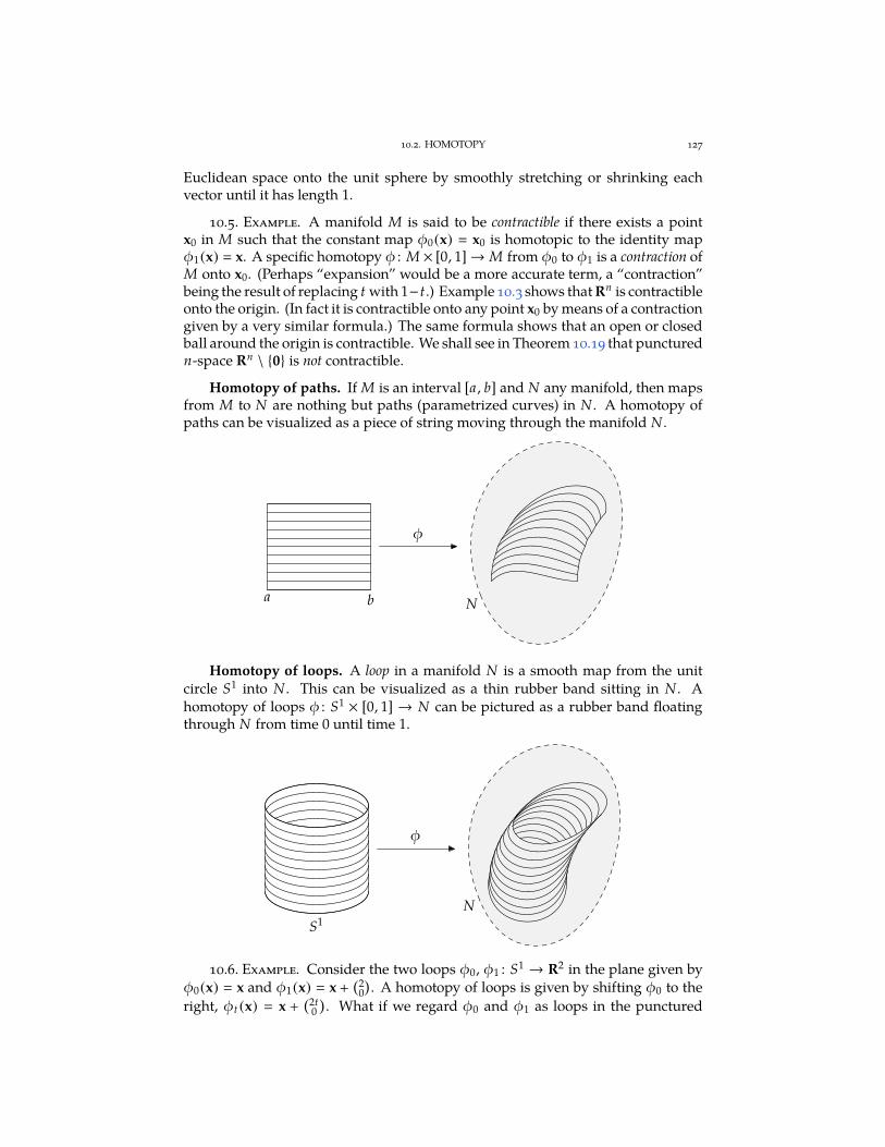
10.2. HOMOTOPY 127
Euclidean space onto the unit sphere by smoothly stretching or shrinking eachvector until it has length 1.
10.5. Example. A manifold M is said to be contractible if there exists a pointx0 in M such that the constant map φ0(x) x0 is homotopic to the identity mapφ1(x) x. A specific homotopy φ : M × [0, 1]→ M from φ0 to φ1 is a contraction ofM onto x0. (Perhaps “expansion” would be a more accurate term, a “contraction”being the result of replacing t with 1−t.) Example 10.3 shows that Rn is contractibleonto the origin. (In fact it is contractible onto any point x0 by means of a contractiongiven by a very similar formula.) The same formula shows that an open or closedball around the origin is contractible. We shall see in Theorem 10.19 that puncturedn-space Rn \ 0 is not contractible.
Homotopy of paths. If M is an interval [a, b] and N any manifold, then mapsfrom M to N are nothing but paths (parametrized curves) in N . A homotopy ofpaths can be visualized as a piece of string moving through the manifold N .
a b N
φ
Homotopy of loops. A loop in a manifold N is a smooth map from the unitcircle S1 into N . This can be visualized as a thin rubber band sitting in N . Ahomotopy of loops φ : S1 × [0, 1] → N can be pictured as a rubber band floatingthrough N from time 0 until time 1.
S1
N
φ
10.6. Example. Consider the two loops φ0, φ1 : S1 → R2 in the plane given byφ0(x) x and φ1(x) x +
(20
)
. A homotopy of loops is given by shifting φ0 to theright, φt (x) x +
(2t0
)
. What if we regard φ0 and φ1 as loops in the punctured
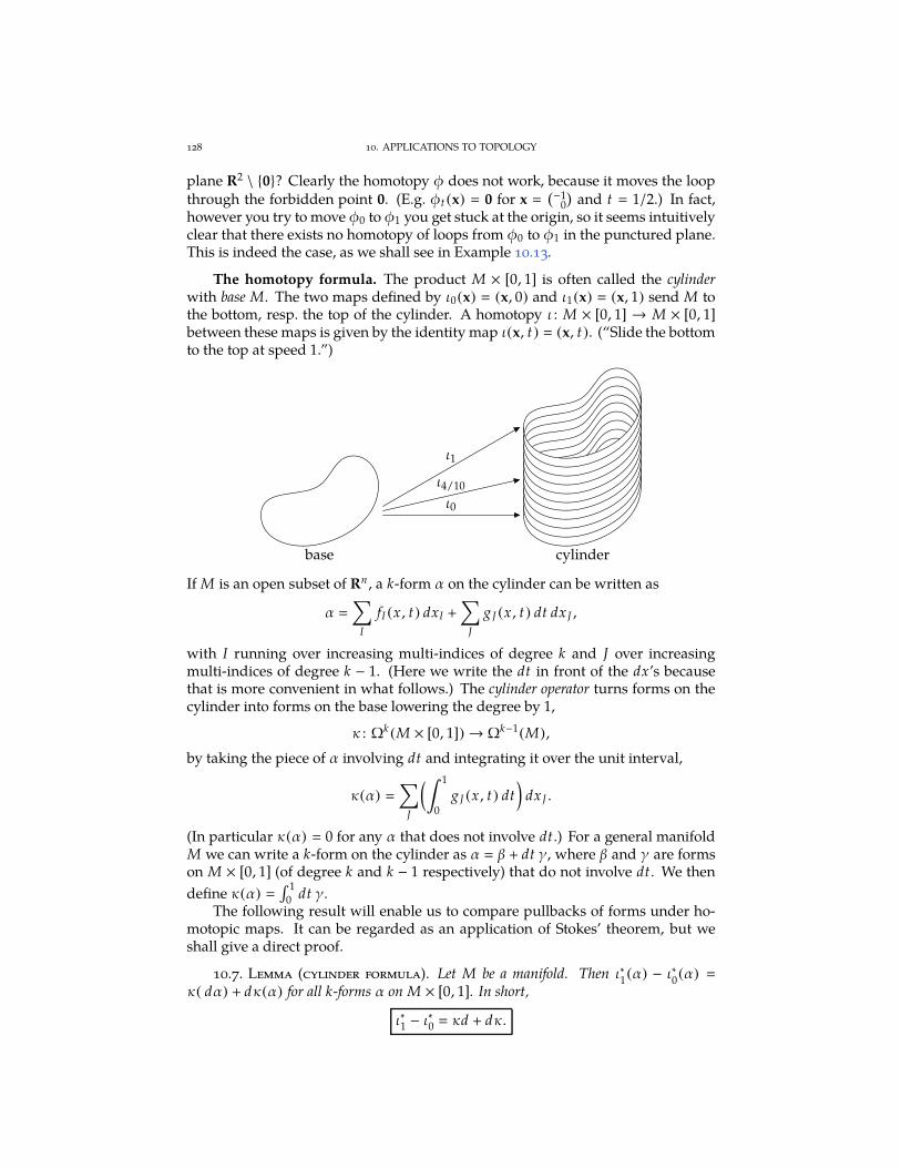
128 10. APPLICATIONS TO TOPOLOGY
plane R2 \ 0? Clearly the homotopy φ does not work, because it moves the loopthrough the forbidden point 0. (E.g. φt (x) 0 for x
(−10
)
and t 1/2.) In fact,however you try to move φ0 to φ1 you get stuck at the origin, so it seems intuitivelyclear that there exists no homotopy of loops from φ0 to φ1 in the punctured plane.This is indeed the case, as we shall see in Example 10.13.
The homotopy formula. The product M × [0, 1] is often called the cylinderwith base M. The two maps defined by ι0(x) (x, 0) and ι1(x) (x, 1) send M tothe bottom, resp. the top of the cylinder. A homotopy ι : M × [0, 1] → M × [0, 1]between these maps is given by the identity map ι(x, t) (x, t). (“Slide the bottomto the top at speed 1.”)
ι0
ι4/10
ι1
base cylinder
If M is an open subset of Rn , a k-form α on the cylinder can be written as
α
∑
I
fI (x , t) dxI +∑
J
g J (x , t) dt dx J ,
with I running over increasing multi-indices of degree k and J over increasingmulti-indices of degree k − 1. (Here we write the dt in front of the dx’s becausethat is more convenient in what follows.) The cylinder operator turns forms on thecylinder into forms on the base lowering the degree by 1,
κ : Ωk (M × [0, 1])→ Ωk−1(M),
by taking the piece of α involving dt and integrating it over the unit interval,
κ(α)
∑
J
(∫ 1
0
g J (x , t) dt)
dx J .
(In particular κ(α) 0 for any α that does not involve dt.) For a general manifoldM we can write a k-form on the cylinder as α β + dt γ, where β and γ are formson M × [0, 1] (of degree k and k − 1 respectively) that do not involve dt. We then
define κ(α)
∫ 1
0 dt γ.The following result will enable us to compare pullbacks of forms under ho-
motopic maps. It can be regarded as an application of Stokes’ theorem, but weshall give a direct proof.
10.7. Lemma (cylinder formula). Let M be a manifold. Then ι∗1(α) − ι∗
0(α)
κ( dα) + dκ(α) for all k-forms α on M × [0, 1]. In short,
ι∗1 − ι∗0 κd + dκ.
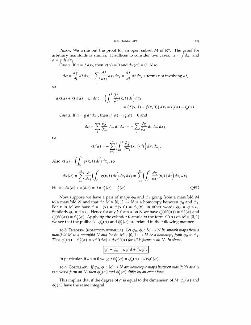
10.2. HOMOTOPY 129
Proof. We write out the proof for an open subset M of Rn . The proof forarbitrary manifolds is similar. It suffices to consider two cases: α f dxI andα g dt dx J .
Case 1. If α f dxI , then κ(α) 0 and dκ(α) 0. Also
dα
∂ f
∂tdt dxI +
∑
i
∂ f
∂xidxi dxI
∂ f
∂tdt dxI + terms not involving dt ,
so
dκ(α) + κ( dα) κ( dα)
(∫ 1
0
∂ f
∂t(x, t) dt
)
dxI
(
f (x, 1) − f (x, 0))
dxI ι∗1(α) − ι∗0(α).
Case 2. If α g dt dx J , then ι∗0(α) ι∗
1(α) 0 and
dα
∑
i
∂g
∂xidxi dt dx J −
∑
i
∂g
∂xidt dxi dx J ,
so
κ(dα) −n∑
i1
(∫ 1
0
∂g
∂xi(x, t) dt
)
dxi dx J .
Also κ(α)
(∫ 1
0
g(x, t) dt)
dx J , so
dκ(α)
n∑
i1
∂
∂xi
(∫ 1
0
g(x, t) dt)
dxi dx J
n∑
i1
(∫ 1
0
∂g
∂xi(x, t) dt
)
dxi dx J .
Hence dκ(α) + κ(dα) 0 ι∗1(α) − ι∗
0(α). QED
Now suppose we have a pair of maps φ0 and φ1 going from a manifold Mto a manifold N and that φ : M × [0, 1] → N is a homotopy between φ0 and φ1.For x in M we have φ ι0(x) φ(x, 0) φ0(x), in other words φ0 φ ι0.Similarly φ1 φ ι1. Hence for any k-form α on N we have ι∗
0(φ∗(α)) φ∗
0(α) and
ι∗1(φ∗(α)) φ∗
1(α). Applying the cylinder formula to the form φ∗(α) on M × [0, 1]
we see that the pullbacks φ∗0(α) and φ∗
1(α) are related in the following manner.
10.8. Theorem (homotopy formula). Let φ0, φ1 : M → N be smooth maps from amanifold M to a manifold N and let φ : M × [0, 1] → N be a homotopy from φ0 to φ1.Then φ∗
1(α) − φ∗
0(α) κφ∗(dα) + dκφ∗ (α) for all k-forms α on N . In short,
φ∗1 − φ∗0 κφ∗d + dκφ∗ .
In particular, if dα 0 we get φ∗1(α) φ∗
0(α) + dκφ∗(α).
10.9. Corollary. If φ0, φ1 : M → N are homotopic maps between manifolds and αis a closed form on N , then φ∗
0(α) and φ∗
1(α) differ by an exact form.
This implies that if the degree of α is equal to the dimension of M, φ∗0(α) and
φ∗1(α) have the same integral.
130 10. APPLICATIONS TO TOPOLOGY
10.10. Theorem. Let M and N be manifolds and let α be a closed n-form on N , wheren dim(M). Suppose M is compact and oriented and without boundary. Let φ0 and φ1
be homotopic maps from M to N . Then∫M
φ∗0(α)
∫M
φ∗1(α).
Proof. By Corollary 10.9, φ∗1(α) −φ∗
0(α) dβ for an n−1-form β on M. Hence
by Stokes’ theorem ∫M
(
φ∗1(α) − φ∗0(α))
∫M
dβ
∫∂M
β 0,
because ∂M is empty. QED
Alternative proof. Here is a proof based on Stokes’ theorem for the manifoldM × [0, 1]. The boundary of M × [0, 1] consists of two copies of M, namely M × 1and M × 0, the first of which is counted with a plus sign and the second with aminus. Therefore, if φ : M × [0, 1]→ N is a homotopy between φ0 and φ1,
0
∫M×[0,1]
φ∗(dα)
∫M×[0,1]
dφ∗(α)
∫∂(M×[0,1])
φ∗(α)
∫M
φ∗1(α) −∫
M
φ∗0(α),
so∫
M φ∗1(α)
∫M φ∗
0(α). QED
10.11. Corollary. Homotopic loops in R2 \ 0 have the same winding number aboutthe origin.
Proof. Let M be the circle S1, N the punctured plane R2 \ 0, and α0 the angleform (−y dx + x dy)/(x2 + y2). Then a map φ from M to N is nothing but a loop inthe punctured plane, and the integral
∫M φ∗(α0) is 2π times the winding number
w(φ, 0). (See Section 4.3.) Thus, if φ0 and φ1 are homotopic loops in N , Theorem10.10 tells us that w(φ0 , 0) w(φ1 , 0). QED
10.12. Example. Unfolding the three self-intersections in the path picturedbelow does not affect its winding number.
0 0
10.13. Example. The two circles φ0 and φ1 of Example 10.6 have windingnumber 1, resp. 0 about the origin and therefore are not homotopic (as loops in thepunctured plane).
10.3. CLOSED AND EXACT FORMS RE-EXAMINED 131
10.3. Closed and exact forms re-examined
The homotopy formula throws light on our old question of when a closedform is exact, which we looked into in Section 2.3. The answer turns out todepend on the “shape” of the manifold on which the forms are defined. On somemanifolds all closed forms (of positive degree) are exact, on others this is true onlyin certain degrees. Failure of exactness is typically detected by integrating over asubmanifold of the correct dimension and finding a nonzero answer. In a certainsense all obstructions to exactness are of this nature. It is to make these statementsprecise that de Rham developed his cohomology theory. We shall not developthis theory in detail, but study a few representative special cases. The matter isexplored in [Fla89] and at a more advanced level in [BT82].
0-forms. A closed 0-form on a manifold is a smooth function f satisfyingd f 0. This means that f is constant (on each connected component of M). If thisconstant is nonzero, then f is not exact (because forms of degree−1 are by definition0). So a closed 0-form is never exact (unless it is 0) for a rather uninteresting reason.
1-forms and simple connectivity. Let us now consider 1-forms on a manifoldM. Theorem 4.7 says that the integral of an exact 1-form along a loop is 0. Witha stronger assumption on the loop the same is true for arbitrary closed 1-forms. Aloop c : S1 → M is null-homotopic if it is homotopic to a constant loop. The integralof a 1-form along a constant loop is 0, so from Theorem 10.10 (where we set the Mof the theorem equal to S1) we get the following.
10.14. Proposition. Let c be a null-homotopic loop in M. Then∫
c α 0 for all closedforms α on M.
A manifold is simply connected if every loop in it is null-homotopic.
10.15. Theorem. All closed 1-forms on a simply connected manifold are exact.
Proof. Let α be a closed 1-form and c a loop in M. Then c is null-homotopic,so
∫c α 0 by Proposition 10.14. The result now follows from Theorem 4.7. QED
10.16. Example. The punctured plane R2 \ 0 is not simply connected, becauseit possesses a nonexact closed 1-form. (See Example 4.6.) In contrast it can beproved that for n ≥ 3 the sphere Sn−1 and punctured n-space Rn \ 0 are simplyconnected. Intuitively, the reason is that in two dimensions a loop that enclosesthe puncture at the origin cannot be crumpled up to a point without getting stuckat the puncture, whereas in higher dimensions there is enough room to slide anyloop away from the puncture and then squeeze it to a point.
The Poincaré lemma. On a contractible manifold all closed forms of positivedegree are exact.
10.17. Theorem (Poincaré lemma). All closed forms of degree k ≥ 1 on a contractiblemanifold are exact.
Proof. Let M be a manifold and let φ : M × [0, 1] → M be a contraction ontoa point x0 in M, i.e. a smooth map satisfying φ(x, 0) x0 and φ(x, 1) x for allx. Let α be a closed k-form on M with k ≥ 1. Then φ∗
1(α) α and φ∗
0(α) 0, so
putting β κφ∗ (α) we get
dβ dκφ∗(α) φ∗1(α) − φ∗0(α) − κdφ∗(α) α.
132 10. APPLICATIONS TO TOPOLOGY
Here we used the homotopy formula, Theorem 10.8, and the assumption thatdα 0. Hence dβ α. QED
The proof provides us with a formula for the “antiderivative”, namely β
κφ∗(α), which can be made quite explicit in certain cases.
10.18. Example. Let M be Rn and let φ(x, t) tx be the radial contraction. Letα
∑
i fi dxi be a 1-form and let g be the function κφ∗ (α). Then
φ∗(α) ∑
i
fi (tx)d(txi ) ∑
i
fi (tx)(xi dt + t dxi ),
so
g κφ∗(α) ∑
i
xi
∫ 1
0
fi (tx) dt .
According to the proof of the Poincaré lemma the function g satisfies dg α,provided that dα 0. We checked this directly in Exercise 4.3.
Another typical application of the Poincaré lemma is showing that a manifoldis not contractible by exhibiting a closed form that is not exact. For example, thepunctured plane R2 \ 0 is not contractible because it possesses a nonexact closed1-form, namely the angle form. (See Example 4.6.) The generalized angle form is then − 1-form α0 on punctured n-space Rn \ 0 defined by
α0
x · ∗dx
‖x‖n.
10.19. Theorem. The generalized angle form α0 is a closed but non-exact n − 1-formon punctured n-space. Hence punctured n-space is not contractible.
Proof. That dα0 0 follows from Exercise 2.20. The n − 1-sphere M Sn−1
has unit normal vector field x, so by Corollary 8.17 on M we have α0 µ, thevolume form. Hence
∫M α0 vol(M) , 0. On the other hand, suppose α0 was
exact, α0 dβ for an n − 1-form β. Then∫M
α0
∫M
dβ
∫∂M
β 0
by Stokes’ theorem, Theorem 9.9. This is a contradiction, so α0 is not exact. It nowfollows from the Poincaré lemma, Theorem 10.17, that Rn \ 0 is not contractible.
QED
A similar argument gives the next result.
10.20. Theorem. Compact orientable manifolds without boundary of dimension ≥ 1are not contractible.
Proof. Let M be a compact orientable manifold of dimension n ≥ 1. Letµ µM be the volume form of M. Then
∫M µ vol(M) , 0. On the other hand,
if M was contractible, then µ would be exact by the Poicaré lemma, so µ dν and∫M µ
∫M dν
∫∂M ν 0 because M has no boundary. This is a contradiction, so
M is not contractible. QED
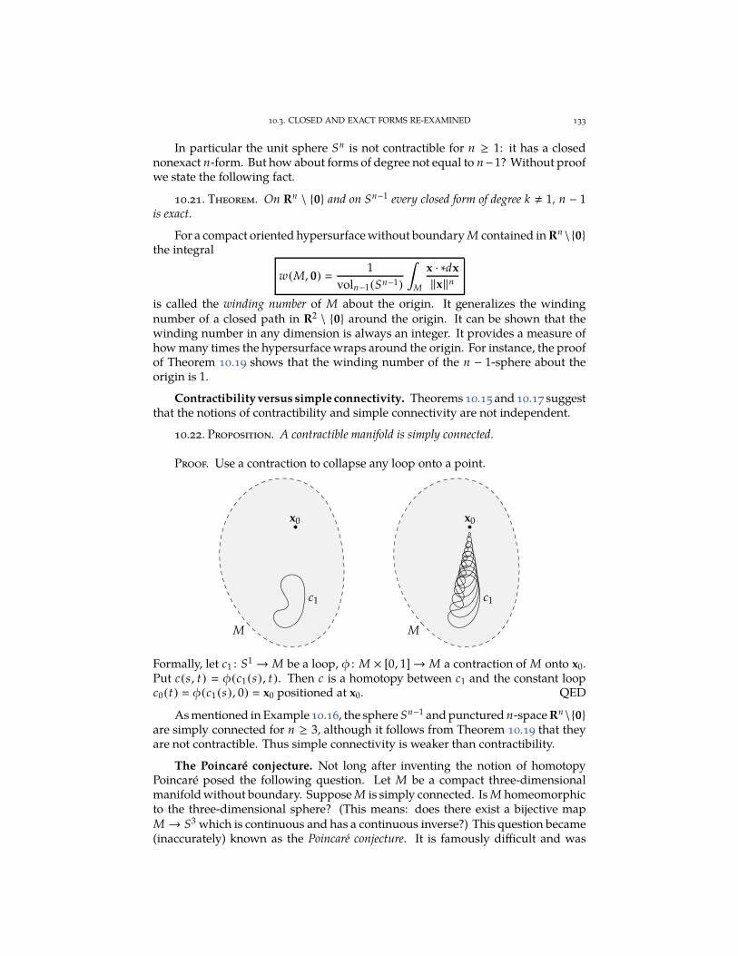
10.3. CLOSED AND EXACT FORMS RE-EXAMINED 133
In particular the unit sphere Sn is not contractible for n ≥ 1: it has a closednonexact n-form. But how about forms of degree not equal to n−1? Without proofwe state the following fact.
10.21. Theorem. On Rn \ 0 and on Sn−1 every closed form of degree k , 1, n − 1is exact.
For a compact oriented hypersurface without boundary M contained in Rn \0the integral
w(M, 0) 1
voln−1(Sn−1)
∫M
x · ∗dx
‖x‖n
is called the winding number of M about the origin. It generalizes the windingnumber of a closed path in R2 \ 0 around the origin. It can be shown that thewinding number in any dimension is always an integer. It provides a measure ofhow many times the hypersurface wraps around the origin. For instance, the proofof Theorem 10.19 shows that the winding number of the n − 1-sphere about theorigin is 1.
Contractibilityversus simple connectivity. Theorems 10.15and 10.17 suggestthat the notions of contractibility and simple connectivity are not independent.
10.22. Proposition. A contractible manifold is simply connected.
Proof. Use a contraction to collapse any loop onto a point.
M
x0
c1
M
x0
c1
Formally, let c1 : S1 → M be a loop, φ : M × [0, 1]→ M a contraction of M onto x0.Put c(s, t) φ(c1(s), t). Then c is a homotopy between c1 and the constant loopc0(t) φ(c1(s), 0) x0 positioned at x0. QED
As mentioned in Example 10.16, the sphere Sn−1 and punctured n-space Rn\0are simply connected for n ≥ 3, although it follows from Theorem 10.19 that theyare not contractible. Thus simple connectivity is weaker than contractibility.
The Poincaré conjecture. Not long after inventing the notion of homotopyPoincaré posed the following question. Let M be a compact three-dimensionalmanifold without boundary. Suppose M is simply connected. Is M homeomorphicto the three-dimensional sphere? (This means: does there exist a bijective mapM → S3 which is continuous and has a continuous inverse?) This question became(inaccurately) known as the Poincaré conjecture. It is famously difficult and was
134 10. APPLICATIONS TO TOPOLOGY
the force that drove many of the developments in twentieth-century topology. Ithas an n-dimensional analogue, called the generalized Poincaré conjecture, whichasks whether every compact n-dimensional manifold without boundary whichis homotopy equivalent to Sn is homeomorphic to Sn . We cannot go into thisfascinating problem in any serious way, other than to report that it has now beencompletely solved. Strangely, the case n ≥ 5 of the generalized Poincaré conjectureconjecture was the easiest and was confirmed by S. Smale in 1960. The case n 4was done by M. Freedman in 1982. The case n 3, the original version of theconjecture, turned out to be the hardest, but was finally confirmed by G. Perelmanin 2002-03. For a discussion and references, see the paper [Mil03] listed in thebibliography.
De Rham cohomology. The distinction between closed and exact differentialforms on a manifold can be encoded in an invariant called de Rham cohomology.To explain this we need to review a little set theory and linear algebra.
Let X be a set. A binary relation ∼ (i.e. a relation among pairs of elements) onX is an equivalence relation if it is
(i) reflexive: x ∼ x;(ii) symmetric: if x ∼ y then y ∼ x;
(iii) transitive: if x ∼ y and y ∼ z then x ∼ z
for all x, y, z ∈ X.
10.23. Example. Consider the following binary relations.(i) Let X R with the order relation ≤ (“less than or equal to”).
(ii) Let X Z. Fix n ∈ Z. Define x ≡ y if x − y is divisible by n (“congruencemodulo n”).
(iii) Let X be the set of all people.(a) Define x ⊲⊳ y if x is a blood relative of y.(b) Define x y if x is a friend of y.
(iv) Let X be the set of straight lines in the plane. Define x ‖ y if x is parallelto y.
Then we have the following table.
reflexive symmetric transitive
(i) Y N Y(ii) Y Y Y(iiia) Y Y ?(iiib) N N N(iv) Y Y Y
Whether relation (iiia) is transitive is a matter of taste. In a broad sense we are allblood relatives of mitochondrial Eve, but perhaps this stretches the definition toofar. Only relations (ii) and (iv) are true equivalence relations.
Let ∼ be an equivalence relation on a set X. The equivalence class of x ∈ X is theset of all y ∈ X that are equivalent to x. Notation:
[x] y ∈ X | y ∼ x .Note that we have [x] [y] if x ∼ y. Any element of an equivalence class iscalled a representative of that class. An equivalence class usually has many different
10.3. CLOSED AND EXACT FORMS RE-EXAMINED 135
representatives. The set of all equivalence classes is called the quotient of X by theequivalence relation and denoted by X/∼.
In Example 10.23(ii) we write Z/n for the quotient. An element of Z/n is aremainder class modulo n,
[i] i, i + n, i − n, i + n, i + 2n, i − 2n, . . . i + kn | k ∈ Z .Example 10.23(iv) comes up in projective geometry. The equivalence class of a
line in the plane is a point at infinity in the plane. If one adds the points at infinityto the plane one arrives at the projective plane.
10.24. Example. Let E be a real vector space. Fix a linear subspace F. Vectors x,y ∈ E are congruent modulo F if x − y ∈ F. Congruence modulo F is an equivalencerelation on E. The equivalence class [x] of x is the affine subspace through x parallel toF. The equivalence class [0] is equal to the linear subspace F itself. We denote thequotient by E/F and call it the quotient of E by F. A basic fact is that E/F is a vectorspace in its own right. The vector space operations are defined by [x] + [y] [x + y]and c[x] [cx] for all x, y ∈ E and c ∈ R. One can check that these operations arewell-defined and obey the axioms of a real vector space. The origin of E/F is theequivalence class [0], and the opposite of a class [x] is the class [−x].
We have the following special case of Example 10.24 in mind. Let M be amanifold and Ωk (M) the vector space of all k-forms on M. Let E be the linearsubspace of Ωk (M) consisting of all closed k-forms,
E α ∈ Ωk (M) | dα 0 ,and let F be the subspace of E consisting of all exact k-forms,
F α ∈ Ωk (M) | α dβ for some β ∈ Ωk−1(M) .The quotient
HkDR(M) E/F
closed k-forms on M
exact k-forms on M
is the de Rham cohomology of M in degree k. Elements of HkDR(M) are equivalence
classes [α] where α is a closed k-form and α ∼ β if α− β is exact. Both vector spacesE and F are usually infinite-dimensional, but it may very well happen that thequotient Hk
DR(M) is finite-dimensional. For any n-manifold M we have Hk (M) 0if k < 0 or k > n. The reason is simply that we don’t have any nonzero forms on Min degrees below 0 or above n. More interesting are the following assertions.
10.25. Theorem. If M is contractible then
HkDR(M)
R if k 0,
0 if k ≥ 1.
Proof. This is a restatement of the Poincaré lemma, Theorem 10.17. QED
10.26. Theorem. Let M be a compact connected oriented n-manifold without bound-ary. Then Hn
DR(M) is 1-dimensional. A basis of HnDR(M) is [µ], the class of the volume
form of M.
We shall not prove this theorem in general (except to note that the class [µ] isnonzero by the proof of Theorem 10.20), but only for the unit circle.
136 10. APPLICATIONS TO TOPOLOGY
10.27. Theorem. H1DR(S1) is 1-dimensional. A basis of H1
DR(S1) is [µ], the class of
the element of arc length of S1.
Proof. The 1-form µ is closed but not exact and therefore defines a nonzeroclass in H1
DR(S1). We need to prove that for every 1-form α on S1 (which isnecessarily closed because dim(S1) 1) there exists a constant k such that [α]
k[µ]. Assuming we could do this, let us first guess what k should be. The equality[α] k[µ] means [α− kµ] [0], i.e. α− kµ is exact, i.e. α kµ+ dg for some smoothfunction g on S1. Integrating over the circle and using Stokes gives∫
S1
α k
∫S1
µ +
∫S1
dg 2πk.
Let us therefore define k (2π)−1∫
S1 α, as we must. Next we determine what gshould be by solving dg α − kµ for g. We do this indirectly by first solving theequation dh c∗(α − kµ), where c(t) (cos t , sin t) is the usual parametrizationof the circle. We have c∗(α) f dt, where f : R→ R is a 2π-periodic function. Theconstant k is given in terms of f by
k
1
2π
∫S1
α
1
2π
∫ 2π
0
c∗(α) 1
2π
∫ 2π
0
f (t) dt . (10.1)
A solution of the equation dh c∗(α − kµ) ( f − k) dt is the function h(t) ∫ t
0 ( f (s) − k) ds
∫ t
0 f (s) ds − kt. This function has the property
h(t + 2π)
∫ t+2π
0
f (s) ds − k(t + 2π)
∫ t
0
f (s) ds − kt +
∫ t+2π
t
f (s) ds − 2πk
h(t) +
∫ 2π
0
f (s) ds − 2πk h(t),
where the last step follows from the periodicity of f and from (10.1). This showsthat h is 2π-periodic, and therefore of the form h(t) g(c(t)), i.e. h c∗(g),for some smooth function g on S1. The equation dh c∗(α − kµ) then becomesc∗(dg) c∗(α − kµ), which implies dg α − kµ because c is a parametrization ofthe circle. QED
Exercises
10.1. Write a formula for the map φ occurring in the proof of Brouwer’s fixed pointtheorem and prove that it is smooth.
10.2. Let x0 be any point in Rn . By analogy with the radial contraction onto the origin,write a formula for radial contraction onto the point x0. Deduce that any open or closed ballcentred at x0 is contractible.
10.3. A subset M of Rn is star-shaped relative to a point x0 ∈ M if for all x ∈ M thestraight line segment joining x0 to x is entirely contained in M. Show that if M is star-shapedrelative to x0, then it is contractible onto x0. Give an example of a contractible set that is notstar-shaped.
10.4. A subset M of Rn is convex if for all x and y in M the straight line segment joiningx to y is entirely contained in M. Prove the following assertions.
(i) M is convex if and only if it is star-shaped relative to each of its points. Give anexample of a star-shaped set that is not convex.
EXERCISES 137
(ii) The closed ball B(ε, x) of radius ε centred at x is convex.(iii) The open ball B(ε, x) of radius ε centred at x is convex.
10.5. Recall that GL(n,R) denotes the general linear group and O(n) the orthogonalgroup. (See Theorem 6.18 and Exercise 6.13.) Define a map φ : GL(n,R) → O(n) byφ(A) Q, where Q is the first factor in the QR-decomposition of A. (See the proof ofTheorem 8.4.) Prove the following assertions.
(i) φ is a retraction.(ii) φ is homotopic to the identity mapping of M.
10.6. Compute the turning number (see Exercise 4.14) of the loopsφ0 andφ1 of Example10.12. Despite the fact that the loops are homotopic they do not have the same turningnumber. Why does this not contradict Theorem 10.10?
10.7. Let k ≥ 1 and let α be the k-form f dxI f dxi1 dxi2 · · · dxikon Rn . Let φ : Rn ×
[0, 1]→ Rn be the radial contraction φ(x, t) tx. Verify that
κφ∗(α)
k∑
m1
(−1)m+1xim
(∫ 1
0tk−1 f (tx) dt
)
dxI\im,
where we have written dxI\imas an abbreviation for dxi1 dxi2 · · · dx im
· · · dxik. Check directly
that dκφ∗ (α) + κdφ∗(α) α.
10.8. Let α f dx dy+g dz dx+h dy dz be a 2-form on R3 and letφ(x, y , z, t) t(x, y , z)
be the radial contraction of R3 onto the origin. Verify that
κφ∗(α)
(∫ 1
0f (tx, t y , tz)t dt
)
(x dy − y dx) +(∫ 1
0g(tx, t y , tz)t dt
)
(z dx − x dz)
+(∫ 1
0h(tx, t y , tz)t dt
)
(y dz − z dy).
10.9. Let α
∑
I fI dxI be a closed k-form whose coefficients fI are smooth functionsdefined on Rn \ 0 that are all homogeneous of the same degree p , −k. Let
β
1
p + k
∑
I
k∑
l1
(−1)l+1xilfI dxi1 dxi2 · · · dx il
· · · dxik.
Show that dβ α. (Use dα 0 and apply the identity proved in Exercise B.6 to each fI ; seealso Exercise 2.9.)
10.10. Let α (2xyz − x2 y) dy dz + (xz2 − y2z) dz dx + (2xyz − xy2) dx dy.
(i) Check that α is closed.(ii) Find a 1-form β such that dβ α.
10.11. Let M and N be manifolds and φ0, φ1 : M → N homotopic maps. Show that∫c φ∗0(α)
∫c φ∗1(α) for all closed k-chains c in M and all closed k-forms α on N .
10.12. Prove that any two maps φ0 and φ1 from M to N are homotopic if M or N iscontractible. (First show that every map M → N is homotopic to a constant map φ(x) y0.)
10.13. Let x0 (2, 0) and let M be the twice-punctured plane R2 \ 0, x0. Let c1, c2 ,c3 : [0, 2π] → M be the loops defined by c1(t) (cos t , sin t), c2(t) (2 + cos t , sin t) andc3(t) (1 + 2 cos t , 2 sin t). Show that c1, c2 and c3 are not homotopic. (Construct a 1-formα on M such that the integrals
∫c1α,
∫c2α and
∫c3α are distinct.)
138 10. APPLICATIONS TO TOPOLOGY
10.14. Let M be a manifold. Let [α] be a class in HkDR
(M) and let [β] be a class in
H lDR
(M). Define the product of [α] and [β] to be the class [α] ·[β] [αβ] ∈ Hk+lDR
(M). Showthat [α] ·[β] is well-defined, i.e. independent of the choice of the representatives of the classes[α] and [β].
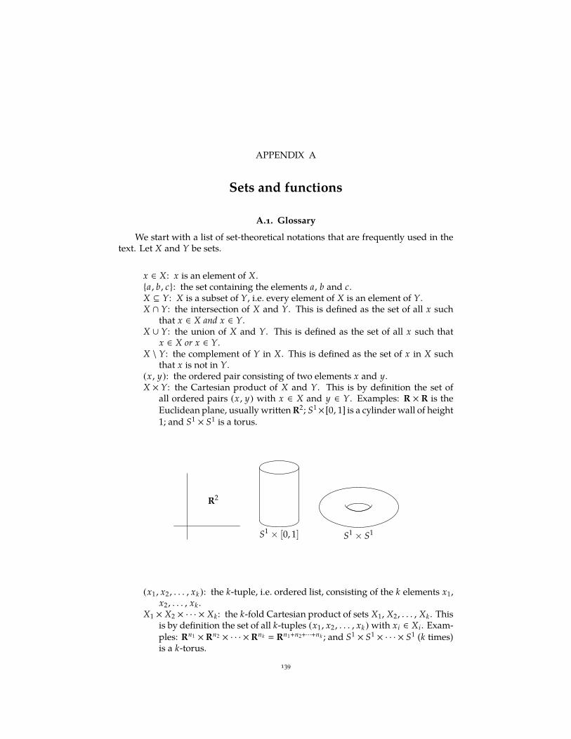
APPENDIX A
Sets and functions
A.1. Glossary
We start with a list of set-theoretical notations that are frequently used in thetext. Let X and Y be sets.
x ∈ X: x is an element of X.a, b, c: the set containing the elements a, b and c.X ⊆ Y: X is a subset of Y, i.e. every element of X is an element of Y.X ∩ Y: the intersection of X and Y. This is defined as the set of all x such
that x ∈ X and x ∈ Y.X ∪ Y: the union of X and Y. This is defined as the set of all x such that
x ∈ X or x ∈ Y.X \ Y: the complement of Y in X. This is defined as the set of x in X such
that x is not in Y.(x , y): the ordered pair consisting of two elements x and y.X × Y: the Cartesian product of X and Y. This is by definition the set of
all ordered pairs (x , y) with x ∈ X and y ∈ Y. Examples: R × R is theEuclidean plane, usually written R2; S1× [0, 1] is a cylinder wall of height1; and S1 × S1 is a torus.
R2
S1× [0, 1] S1
× S1
(x1 , x2 , . . . , xk ): the k-tuple, i.e. ordered list, consisting of the k elements x1,x2 , . . . , xk .
X1 × X2 × · · · × Xk: the k-fold Cartesian product of sets X1, X2, . . . , Xk . Thisis by definition the set of all k-tuples (x1 , x2 , . . . , xk ) with xi ∈ Xi. Exam-ples: Rn1 ×Rn2 × · · · ×Rnk
Rn1+n2+···+nk ; and S1 × S1 × · · · × S1 (k times)is a k-torus.
139
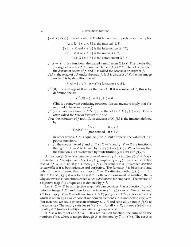
140 A. SETS AND FUNCTIONS
x ∈ X | P(x) : the set of all x ∈ X which have the property P(x). Examples:
x ∈ R | 1 ≤ x < 3 is the interval [1, 3),
x | x ∈ X and x ∈ Y is the intersection X ∩ Y,
x | x ∈ X or x ∈ Y is the union X ∪ Y,
x ∈ X | x < Y is the complement X \ Y.
f : X → Y: f is a function (also called a map) from X to Y. This means thatf assigns to each x ∈ X a unique element f (x) ∈ Y. The set X is calledthe domain or source of f , and Y is called the codomain or target of f .
f (A): the image of a A under the map f . If A is a subset of X, then its imageunder f is by definition the set
f (A) y ∈ Y | y f (x) for some x ∈ A .f −1(B): the preimage of B under the map f . If B is a subset of Y, this is by
definition the set
f −1(B) x ∈ X | f (x) ∈ B .(This is a somewhat confusing notation. It is not meant to imply that f isrequired to have an inverse.)
f −1(c): an abbreviation for f −1(c), i.e. the set x ∈ X | f (x) c . This isoften called the fibre or level set of f at c.
f |A: the restriction of f to A. If A is a subset of X, f |A is the function definedby
( f |A)(x)
f (x) if x ∈ A,
not defined if x < A.
In other words, f |A is equal to f on A, but “forgets” the values of f atpoints outside A.
g f : the composition of f and g. If f : X → Y and g : Y → Z are functions,then g f : X → Z is defined by (g f (x) g( f (x)). We often say thatthe function g f is obtained by “substituting y f (x) into g(y)”.
A function f : X → Y is injective or one-to-one if x1 , x2 implies f (x1) , f (x2).(Equivalently, f is injective if f (x1) f (x2) implies x1 x2.) It is called surjectiveor onto if f (X) Y, i.e. if y ∈ Y then y f (x) for some x ∈ X. It is called bijectiveor invertible if it is both injective and surjective. The function f is bijective if andonly if it has an inverse, that is a map g : Y → X satisfying both g( f (x)) x forall x ∈ X and f (g(y)) y for all y ∈ Y. Both conditions must be satisfied; that’swhy an inverse is sometimes called a two-sided inverse for emphasis. The inverse ofa bijective map f is unique and is denoted by f −1.
Let f : X → Y be an injective map. We can consider f as a bijection from Xonto the image f (X) and then form the inverse f −1 : f (X) → X. We can extendf −1 to a map g : Y → X as follows: for y ∈ f (X) put g(y) f −1(y). For each y ∈ Ywhich is not in f (X) we choose at random an element x ∈ X and define g(y) x.(For instance, we could choose an arbitrary x0 ∈ X and send all y’s not in f (X) tothe same x0.) The map g satisfies g( f (x)) x for all x ∈ X, but not f (g(y)) yfor all y ∈ Y (unless f is bijective). We call g a left inverse of f .
If X is a finite set and f : X → R a real-valued function, the sum of all thenumbers f (x), where x ranges through X, is denoted by
∑
x∈X f (x). The set X is
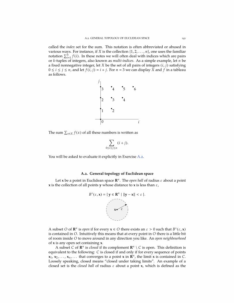
A.2. GENERAL TOPOLOGY OF EUCLIDEAN SPACE 141
called the index set for the sum. This notation is often abbreviated or abused invarious ways. For instance, if X is the collection 1, 2, . . . , n, one uses the familiarnotation
∑ni1 f (i). In these notes we will often deal with indices which are pairs
or k-tuples of integers, also known as multi-indices. As a simple example, let n bea fixed nonnegative integer, let X be the set of all pairs of integers (i, j) satisfying0 ≤ i ≤ j ≤ n, and let f (i, j) i + j. For n 3 we can display X and f in a tableauas follows.
i
j
0
1
2
3
2
3
4
4
5 6
The sum∑
x∈X f (x) of all these numbers is written as
∑
0≤i≤ j≤n
(i + j).
You will be asked to evaluate it explicitly in Exercise A.2.
A.2. General topology of Euclidean space
Let x be a point in Euclidean space Rn . The open ball of radius ε about a pointx is the collection of all points y whose distance to x is less than ε,
B(ε, x) y ∈ Rn | ‖y − x‖ < ε .
x ε
A subset O of Rn is open if for every x ∈ O there exists an ε > 0 such that B(ε, x)
is contained in O. Intuitively this means that at every point in O there is a little bitof room inside O to move around in any direction you like. An open neighbourhoodof x is any open set containing x.
A subset C of Rn is closed if its complement Rn \ C is open. This definition isequivalent to the following: C is closed if and only if for every sequence of pointsx1, x2, . . . , xn , . . . that converges to a point x in Rn , the limit x is contained in C.Loosely speaking, closed means “closed under taking limits”. An example of aclosed set is the closed ball of radius ε about a point x, which is defined as the
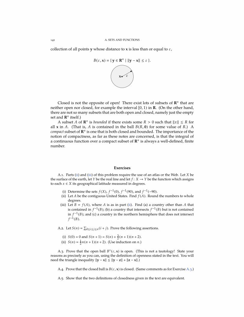
142 A. SETS AND FUNCTIONS
collection of all points y whose distance to x is less than or equal to ε,
B(ε, x) y ∈ Rn | ‖y − x‖ ≤ ε .
x ε
Closed is not the opposite of open! There exist lots of subsets of Rn that areneither open nor closed, for example the interval [0, 1) in R. (On the other hand,there are not so many subsets that are both open and closed, namely just the emptyset and Rn itself.)
A subset A of Rn is bounded if there exists some R > 0 such that ‖x‖ ≤ R forall x in A. (That is, A is contained in the ball B(R, 0) for some value of R.) Acompact subset of Rn is one that is both closed and bounded. The importance of thenotion of compactness, as far as these notes are concerned, is that the integral ofa continuous function over a compact subset of Rn is always a well-defined, finitenumber.
Exercises
A.1. Parts (ii) and (iii) of this problem require the use of an atlas or the Web. Let X bethe surface of the earth, let Y be the real line and let f : X → Y be the function which assignsto each x ∈ X its geographical latitude measured in degrees.
(i) Determine the sets f (X), f −1(0), f −1(90), and f −1(−90).(ii) Let A be the contiguous United States. Find f (A). Round the numbers to whole
degrees.(iii) Let B f (A), where A is as in part (ii). Find (a) a country other than A that
is contained in f −1(B); (b) a country that intersects f −1(B) but is not contained
in f −1(B); and (c) a country in the northern hemisphere that does not intersect
f −1(B).
A.2. Let S(n) ∑
0≤i≤ j≤n (i + j). Prove the following assertions.
(i) S(0) 0 and S(n + 1) S(n) + 32 (n + 1)(n + 2).
(ii) S(n) 12 n(n + 1)(n + 2). (Use induction on n.)
A.3. Prove that the open ball B(ε, x) is open. (This is not a tautology! State yourreasons as precisely as you can, using the definition of openness stated in the text. You willneed the triangle inequality ‖y − x‖ ≤ ‖y − z‖ + ‖z − x‖.)
A.4. Prove that the closed ball is B(ε, x) is closed. (Same comments as for Exercise A.3.)
A.5. Show that the two definitions of closedness given in the text are equivalent.
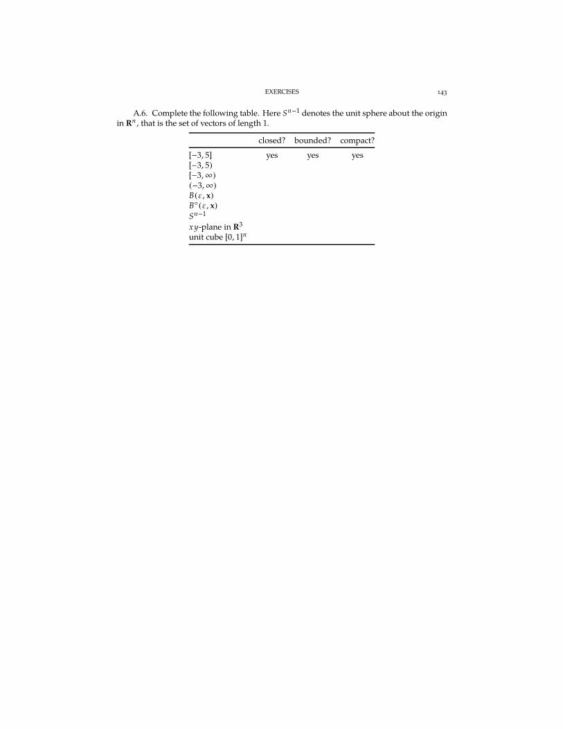
EXERCISES 143
A.6. Complete the following table. Here Sn−1 denotes the unit sphere about the originin Rn , that is the set of vectors of length 1.
closed? bounded? compact?
[−3, 5] yes yes yes[−3, 5)
[−3,∞)
(−3,∞)
B(ε, x)
B(ε, x)
Sn−1
xy-plane in R3
unit cube [0, 1]n

APPENDIX B
Calculus review
This appendix is a brief review of some single- and multi-variable calculusneeded in the study of manifolds. References for this material are [Edw94], [HH09]and [MT11].
B.1. The fundamental theorem of calculus
Suppose that F is a differentiable function of a single variable x and that thederivative f F′ is continuous. Let [a, b] be an interval contained in the domainof F. The fundamental theorem of calculus says that
∫ b
a
f (t) dt F(b) − F(a). (B.1)
There are two useful alternative ways of writing this theorem. Replacing b with xand differentiating with respect to x we find
d
dx
∫ x
a
f (t) dt f (x). (B.2)
Writing g instead of F and g′ instead of f and adding g(a) to both sides in formula(B.1) we get
g(x) g(a) +
∫ x
a
g′(t) dt . (B.3)
Formulæ (B.1)–(B.3) are equivalent, but they emphasize different aspects of thefundamental theorem of calculus. Formula (B.1) is a formula for a definite integral:it tells you how to find the (oriented) surface area between the graph of the functionf and the x-axis. Formula (B.2) says that the integral of a continuous function isa differentiable function of the upper limit; and the derivative is the integrand.Formula (B.3) is an “integral formula”, which expresses the function g in terms ofthe value g(a) and the derivative g′. (See Exercise B.1 for an application.)
B.2. Derivatives
Let φ1, φ2 , . . . , φm be functions of n variables x1, x2 , . . . , xn . As usual we write
x
*....,
x1
x2
...xn
+////-, φ(x)
*....,
φ1(x)
φ2(x)...
φm (x)
+////-,
and view φ(x) as a single map from Rn to Rm . (In calculus the word “map” is oftenused for vector-valued functions, while the word “function” is generally reserved
145
146 B. CALCULUS REVIEW
for real-valued functions.) The most basic way to differentiate a map φ from Rn toRm is to form a limit of the kind
dφ(x + tv)
dt
t0 lim
t→0
φ(x + tv) − φ(x)
t. (B.4)
If this limit exists, it is called the directional derivative of φ at x along v. The expressionx+ tv as a function of t parametrizes a straight line in Rn passing through the pointx in the direction of the vector v. The directional derivative (B.4) measures the rateof change of φ along this straight line. Since φ(x + tv) − φ(x) is a vector in Rm forall t, the directional derivative is likewise a vector in Rm .
If the map φ is not defined everywhere but only on a subset U of Rn , it maybe difficult to make sense of the limit (B.4). Let x be in the domain U of φ. Theproblem is that x + tv may not be in U for all t , 0, so that we cannot evaluateφ(x + tv). The solution is to assume that U is an open subset of Rn . Given anydirection vector v ∈ Rn , we can then find a number ε > 0 such that the pointsx + tv are contained in U for −ε < t < ε. Therefore φ(x + tv) is well-defined for−ε < t < ε and we can legitimately ask whether the limit (B.4) exists.
The partial derivatives of φ at x are by definition the directional derivatives
∂φ
∂x j(x)
dφ(x + te j )
dt
t0, (B.5)
where
e1
*.........,
100...00
+/////////-
, e2
*.........,
010...00
+/////////-
, . . . , en
*.........,
000...01
+/////////-
are the standard basis vectors of Rn , i.e. the columns of the identity n × n-matrix.We can write the partial derivative in components as follows:
∂φ
∂x j(x)
*........,
∂φ1
∂x j(x)
∂φ2
∂x j(x)
...∂φm
∂x j(x)
+////////-
.
The total derivative or Jacobi matrix of φ at x is obtained by lining these columns upin an m × n-matrix
Dφ(x)
*.......,
∂φ1
∂x1(x)
∂φ1
∂x2(x) . . .
∂φ1
∂xn(x)
∂φ2
∂x1(x)
∂φ2
∂x2(x) . . .
∂φ2
∂xn(x)
......
...∂φm
∂x1(x)
∂φm
∂x2(x) . . .
∂φm
∂xn(x)
+///////-
.
We say that the mapφ is continuously differentiable or C1 if the partial derivatives
∂φi
∂x j(x)
B.2. DERIVATIVES 147
are well-defined for all x in the domain U of φ and depend continuously on x forall i 1, 2, . . . , n and j 1, 2, . . . , m. If the second partial derivatives
∂2φi
∂x j∂xk(x)
exist for all x ∈ U and are continuous for all i 1, 2, . . . , n and j, k 1, 2, . . . , m,then φ is called twice continuously differentiable or C2. Likewise, if all r-fold partialderivatives
∂rφi
∂x j1∂x j2 · · · ∂x jr
(x)
exist and are continuous, then φ is r times continuously differentiable or Cr . If φ is Cr
for all r ≥ 1, then we say that φ is infinitely many times differentiable, or C∞, or smooth.This means that φ can be differentiated arbitrarily many times with respect to anyof the variables. Smooth functions include such familiar one-variable functionsas polynomials, exponentials, logarithms and trig functions. (Of course for logand tan one must make the proviso that they are smooth only on their domain ofdefinition.)
The following useful fact says that any directional derivative can be expressedas a linear combination of partial derivatives. The proof is Exercise B.4.
B.1. Lemma. Let U be an open subset of Rn and let φ : U → Rm be a C1 map. Letx ∈ U and v ∈ Rn . Then the directional derivative of φ at x along v exists and is equal to
dφ(x + tv)
dt
t0 Dφ(x)v,
the vector in Rm obtained by multiplying the matrix Dφ(x) by the vector v.
Velocity vectors. Suppose n 1. Then φ is a vector-valued function of onevariable x, called a path or parametrized curve in Rm . The matrix Dφ(x) consists ofa single column vector, called the velocity vector, and is usually denoted simply byφ′(x).
Gradients. Suppose m 1. Then φ is a scalar-valued function of n variablesand Dφ(x) is a single row vector. The transpose matrix of Dφ(x) is therefore acolumn vector, called the gradient of φ:
Dφ(x)T grad(φ)(x).
The directional derivative of φ along v can then be written as an inner product,
Dφ(x)v grad(φ)(x)T v grad(φ)(x) · v.There is an important characterization of the gradient, which is based on thefamiliar identity a · b ‖a‖ ‖b‖ cos θ. Here 0 ≤ θ ≤ π is the angle subtended bya and b. Let us fix a point x in the domain of φ and let us consider all possibledirectional derivatives of φ at x along unit vectors v (i.e. vectors of length 1). Then
Dφ(x)v grad(φ)(x) · v ‖grad(φ)(x)‖ cos θ,
where θ is the angle between grad(φ)(x) and v. So Dφ(x)v takes on its maximalvalue if cos θ 1, i.e. θ 0. This means that v points in the same direction asgrad(φ)(x). Thus the direction of the vector grad(φ)(x) is the direction of steepestascent, i.e. in which φ increases fastest, and the magnitude of grad(φ)(x) is equal
148 B. CALCULUS REVIEW
to the directional derivative Dφ(x)v, where v is the unit vector pointing alonggrad(φ)(x).
B.3. The chain rule
Recall that if A, B and C are sets and φ : A → B and ψ : B → C are maps, wecan apply ψ after φ to obtain the composite map (ψ φ)(x) ψ(φ(x)).
B.2. Theorem (chain rule). Let U ⊆ Rn and V ⊆ Rm be open and let φ : U → V
and ψ : V → Rl be Cr . Then ψ φ is Cr and
D(ψ φ)(x) Dψ(φ(x))Dφ(x)
for all x ∈ U .
Here Dψ(φ(x))Dφ(x) denotes the composition or the product of the l × m-matrix Dψ(φ(x)) and the m × n-matrix Dφ(x).
B.3. Example. In the one-variable case n m l 1 the derivatives Dφ andDψ are 1 × 1-matrices (φ′(x)) and (ψ′(y)), and matrix multiplication is ordinarymultiplication, so we get the usual chain rule
(ψ φ)′(x) ψ′(φ(x))φ′(x).
B.4. Example. Let U be an open subset of Rn and let φ : U → Rm be C1. Let Ibe an open interval and let c : I → U be a path in U . Then φ c is a path in Rm .Suppose that at time t0 ∈ I the path c passes through the point c(t0) x at velocityc′(t0) v. How to compute the velocity vector of the composite path φ c at timet0? The chain rule gives
(φ c)′(t) D(φ c)(t) Dφ(c(t))Dc(t) Dφ(c(t))c′(t)
for all t ∈ I. Setting t t0 gives (φ c)′(t0) Dφ(x)v.
Let us write out a formula for the (i, j)-th entry of the Jacobi matrix of ψ φ.The i-th component of the map ψ φ is ψi φ, so the (i, j)-th entry of D(ψ φ)(x)
is the partial derivative∂(ψi φ)
∂x j(x).
According to Theorem B.2 this entry can be computed by multiplying the i-th rowof Dψ(φ(x)), which is
(∂ψi
∂y1(φ(x))
∂ψi
∂y2(φ(x)) · · · ∂ψ
∂ym(φ(x))
)
,
by the j-th column of Dφ(x), which is
*........,
∂φ1
∂x j(x)
∂φ2
∂x j(x)
...∂φm
∂x j(x)
+////////-
.
This gives the formula
∂(ψi φ)
∂x j(x)
m∑
k1
∂ψi
∂yk(φ(x))
∂φk
∂x j(x).
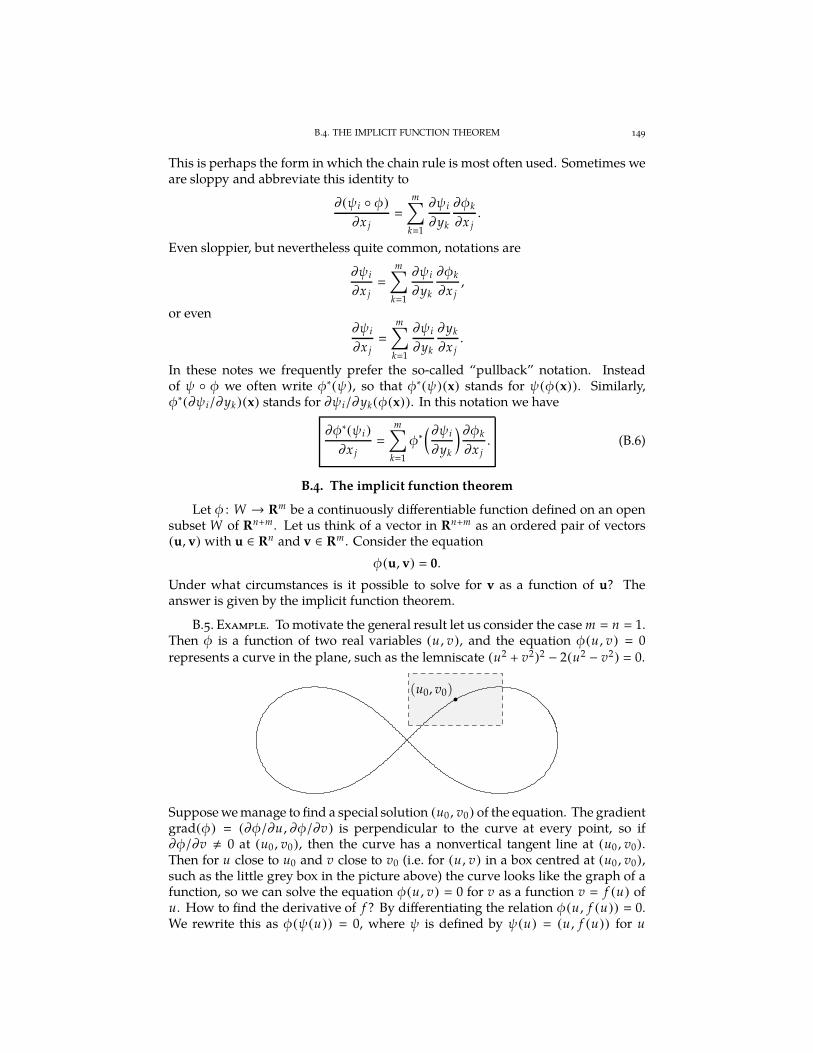
B.4. THE IMPLICIT FUNCTION THEOREM 149
This is perhaps the form in which the chain rule is most often used. Sometimes weare sloppy and abbreviate this identity to
∂(ψi φ)
∂x j
m∑
k1
∂ψi
∂yk
∂φk
∂x j.
Even sloppier, but nevertheless quite common, notations are
∂ψi
∂x j
m∑
k1
∂ψi
∂yk
∂φk
∂x j,
or even∂ψi
∂x j
m∑
k1
∂ψi
∂yk
∂yk
∂x j.
In these notes we frequently prefer the so-called “pullback” notation. Insteadof ψ φ we often write φ∗(ψ), so that φ∗(ψ)(x) stands for ψ(φ(x)). Similarly,φ∗(∂ψi/∂yk)(x) stands for ∂ψi/∂yk(φ(x)). In this notation we have
∂φ∗(ψi )
∂x j
m∑
k1
φ∗( ∂ψi
∂yk
) ∂φk
∂x j. (B.6)
B.4. The implicit function theorem
Let φ : W → Rm be a continuously differentiable function defined on an opensubset W of Rn+m. Let us think of a vector in Rn+m as an ordered pair of vectors(u, v) with u ∈ Rn and v ∈ Rm . Consider the equation
φ(u, v) 0.
Under what circumstances is it possible to solve for v as a function of u? Theanswer is given by the implicit function theorem.
B.5. Example. To motivate the general result let us consider the case m n 1.Then φ is a function of two real variables (u, v), and the equation φ(u, v) 0
represents a curve in the plane, such as the lemniscate (u2 + v2)2 − 2(u2 − v2) 0.
(u0, v0)
Suppose we manage to find a special solution (u0 , v0) of the equation. The gradientgrad(φ) (∂φ/∂u, ∂φ/∂v) is perpendicular to the curve at every point, so if∂φ/∂v , 0 at (u0 , v0), then the curve has a nonvertical tangent line at (u0 , v0).Then for u close to u0 and v close to v0 (i.e. for (u, v) in a box centred at (u0 , v0),such as the little grey box in the picture above) the curve looks like the graph of afunction, so we can solve the equation φ(u, v) 0 for v as a function v f (u) ofu. How to find the derivative of f ? By differentiating the relation φ(u, f (u)) 0.We rewrite this as φ(ψ(u)) 0, where ψ is defined by ψ(u) (u, f (u)) for u
150 B. CALCULUS REVIEW
in an open interval I containing u0. According to the chain rule, Theorem B.2,D(φ ψ)(u) Dφ(ψ(u)Dψ(u). We have
Dφ
(
uv
)
(∂φ∂u (u, v)
∂φ∂v (u, v)
)
, Dψ(u)
(
1f ′(u)
)
,
and therefore
D(φ ψ)(u) ∂φ
∂u(u, f (u)) +
∂φ
∂v(u, f (u)) f ′ (u).
The relation φ(u, f (u)) 0 (which holds for all u ∈ I) tells us that D(φ ψ)(u) 0for u ∈ I. Solving for f ′ gives the implicit differentiation formula
f ′(u) −∂φ
∂u(u, f (u))
/ ∂φ
∂v(u, f (u)).
For general m and n we form the Jacobi matrices of φ with respect to the u-and v-variables separately,
Duφ
*....,
∂φ1
∂u1. . .
∂φ1
∂un
......
∂φm
∂u1. . .
∂φm
∂un
+////-, Dvφ
*....,
∂φ1
∂v1. . .
∂φ1
∂vm
......
∂φm
∂v1. . .
∂φm
∂vm
+////-.
Observe that the matrix Dvφ is square. We are in business if we have a point(u0, v0) at which φ is 0 and Dvφ is invertible.
B.6. Theorem (implicit function theorem). Let φ : W → Rm be Cr , where Wis open in Rn+m . Suppose that (u0 , v0) ∈ W is a point such that φ(u0 , v0) 0 andDvφ(u0 , v0) is invertible. Then there are open neighbourhoods U ⊆ Rn of u0 andV ⊆ Rm of v0 such that for each u ∈ U there exists a unique v f (u) ∈ V satisfyingφ(u, f (u)) 0. The function f : U → V is Cr with derivative given by implicitdifferentiation:
D f (u) −Dvφ(u, v)−1Duφ(u, v)v f (u)
for all u ∈ U .
As a special case we take φ to be of the form φ(u, v) g(v) − u, whereg : W → Rn is a given function with W open in Rn . Solving φ(u, v) 0 hereamounts to inverting the function g. Moreover, Dvφ D g, so the implicit functiontheorem yields the following result.
B.7. Theorem (inverse function theorem). Let g : W → Rn be continuouslydifferentiable, where W is open in Rn . Suppose that v0 ∈ W is a point such that D g(v0)
is invertible. Then there is an open neighbourhood U ⊆ Rn of v0 such that g(U) isan open neighbourhood of g(v0) and the map g : U → g(U) is invertible. The inverseg−1 : V → U is continuously differentiable with derivative given by
D g−1(u) D g(v)−1vg−1 (u)
for all v ∈ V.
Again let us spell out the one-variable case n 1. Invertibility of D g(v0)
simply means that g′(v0) , 0. This implies that near v0 the function g is strictlymonotone increasing (if g′(v0) > 0) or decreasing (if g′(v0) < 0). Therefore if I is
EXERCISES 151
a sufficiently small open interval around u0, then g(I) is an open interval aroundg(u0) and the restricted function g : I → g(I) is invertible. The inverse functionhas derivative
(g−1)′(u) 1
g′(v),
with v g−1(u).
B.8. Example (square roots). Let g(v) v2. Then g′(v0) , 0 whenever v0 , 0.For v0 > 0 we can take I (0,∞). Then g(I) (0,∞), g−1(u)
√u, and (g−1)′(u)
1/(2√
u). For v0 < 0 we can take I (−∞, 0). Then g(I) (0,∞), g−1(u) −√
u,and (g−1)′(u) −1/(2
√u). In a neighbourhood of 0 it is not possible to invert g.
B.5. The substitution formula for integrals
Let V be an open subset of Rn and let f : V → R be a function. Suppose wewant to change the variables in the integral
∫V f (y) dy. (This is shorthand for an
n-fold integral over y1, y2 , . . . , yn .) This means we substitute y p(x), wherep : U → V is a map from an open U ⊆ Rn to V. Under a suitable hypothesis wecan change the integral over y to an integral over x.
B.9. Theorem (change of variables formula). Let U and V be open subsets of Rn
and let p : U → V be a map. Suppose that p is bijective and that p and its inverse arecontinuously differentiable. Then for any integrable function f we have
∫V
f (y) dy
∫U
f (p(x)) |det(Dp(x)) | dx.
Again this should look familiar from one-variable calculus: if p : (a, b) → (c, d)
is C1 and has a C1 inverse, then∫ d
c
f (y) dy
∫ b
a f (p(x))p′(x) dx if p is increasing,∫ a
b f (p(x))p′(x) dx if p is decreasing.
This can be written succinctly as∫ d
c f (y) dy
∫ b
a f (p(x)) |p′(x) | dx, which looksmore similar to the multidimensional case.
Exercises
B.1. Let g : [a, b] → R be a Cn+1-function, where n ≥ 0. Suppose a ≤ x ≤ b and puth x − a.
(i) By changing variables in the fundamental theorem of calculus (B.3) show that
g(x) g(a) + h
∫ 1
0g′(a + th) dt.
(ii) Show that
g(x) g(a) + h(t − 1)g′(a + th)10 + h2
∫ 1
0(1 − t)g′′(a + th) dt
g(a) + hg′ (a) + h2
∫ 1
0(1 − t)g′′(a + th) dt.
(Integrate the formula in part (i) by parts and don’t forget to use the chain rule.)
152 B. CALCULUS REVIEW
(iii) By induction on n deduce from part (ii) that
g(x)
n∑
k0
g(k) (a)
k!hk +
hn+1
n!
∫ 1
0(1 − t)n g(n+1) (a + th) dt.
This is Taylor’s formula with integral remainder term.
B.2. Let φ : R → R be the function defined by φ(x) x |x |. Show that φ is C1 but not
C2. For each r ≥ 1 give an example of a function which is Cr but not Cr+1.
B.3. Define a function f : R→ R by f (0) 0 and f (x) e−1/x2for x , 0.
(i) Show that f is differentiable at 0 and that f ′(0) 0. (Use the definition of thederivative,
f ′(0) limx→0
f (x) − f (0)
x.)
(ii) Show that f is smooth and that f (n) (0) 0 for all n. (By induction on n, provethe following assertion:
f (n) (x)
0 if x 0,
gn (1/x)e−1/x2if x , 0,
where, for each n ≥ 0, gn (1/x) is a certain polynomial in 1/x, which you neednot determine explicitly.)
(iii) Plot the function f over the interval −5 ≤ x ≤ 5. Using software or a graphingcalculator is fine, but pay special attention to the behaviour near x 0.
B.4. (i) Let x and v be vectors in Rn . Define a path c : R→ Rn by c(t) x + tv.Find c′(t).
(ii) Prove Lemma B.1. (Let φ : U → Rm be a C1 map, where U is open in Rn .Combine the result of part (i) with the formula of Example B.4.)
B.5. According to Newton’s law of gravitation, a particle of mass m1 placed at the origin
in R3 exerts a force on a particle of mass m2 placed at x ∈ R3 \ 0 equal to
F −Gm1m2
‖x‖3x,
where G is a constant of nature. Show that F is the gradient of f (x) Gm1m2/‖x‖.
B.6. A function f : Rn \ 0 → R is homogeneous of degree p if f (tx) tp f (x) for allx ∈ Rn \ 0 and t > 0. Here p is a real constant.
(i) Show that the functions f1(x, y) (x2 − xy)/(x2 + y2), f2(x, y)
√
x3 + y3,
f3(x, y , z) (x2z6 + 3x4 y2z2)−√
2 are homogeneous. What are their degrees?(ii) Let f be a homogeneous function of degree p. Assume that f is defined at 0 and
continuous everywhere. Also assume f (x) , 0 for at least one x ∈ Rn . Show thatp ≥ 0. Show that f is constant if p 0.
(iii) Show that if f is homogeneous of degree p and smooth, then
n∑
i1
xi∂ f
∂xi(x) p f (x).
(Differentiate the relation f (tx) tp f (x) with respect to t.)
B.7. A function f : Rn \ 0 → R is quasihomogeneous of degree p if there exist realconstants a1, a2 , . . . , an with the property that
f (ta1 x1 , ta2 x2 , . . . , t
an xn ) tp f (x)
EXERCISES 153
for all x ∈ Rn \ 0 and t > 0. Suppose that f is quasihomogeneous of degree p and smooth.
Show that∑n
i1 ai xi∂ f∂xi
(x) p f (x).
B.8. Define a map ψ from Rn−1 to Rn by
ψ(t) 1
‖t‖2 + 1
(
2t + (‖t‖2 − 1)en)
.
(Here we regard a point t (t1 , t2 , . . . , tn−1) in Rn−1 as a point in Rn by identifying it with(t1 , t2 , . . . , tn−1 , 0).)
(i) Show that ψ(t) lies on the unit sphere Sn−1 about the origin.(ii) Show that ψ(t) is the intersection point of the sphere and the line through the
points en and t.(iii) Compute Dψ(t).
(iv) Let X be the sphere punctured at the “north pole”, X Sn−1 \ en . Stereographic
projection from the north pole is the map φ : X → Rn−1 given by φ(x) (1 −xn )−1(x1 , x2 , . . . , xn−1)T . Show that φ is a two-sided inverse of ψ.
(v) Draw diagrams illustrating the maps φ and ψ for n 2 and n 3.(vi) Now let y be any point on the sphere and let P the hyperplane perpendicular to
y. (A hyperplane in Rn is a linear subspace of dimension n − 1.) The stereographicprojection from y of any point x in the sphere distinct from y is defined as theunique intersection point of the line joining y to x and the hyperplane P. This
defines a map φ : Sn−1 \ y → P. The point y is called the centre of the projection.Write a formula for the stereographic projection φ from the south pole −en and
for its inverse ψ : Rn−1 → Sn−1.
B.9. Let φ : Rn → Rm be a C1 map. Prove the following assertions.
(i) φ is constant if and only if Dφ(x) 0 for all x ∈ Rn .(ii) φ is linear if and only if Dφ(x)v φ(v) for all x and v in Rn .
B.10. A map φ : Rn → Rm is called even if φ(−x) φ(x) for all x in Rn . Find Dφ(0) if
φ is even and C1.
B.11. Let f : R2 → R be a smooth function which satisfies f (x, y) − f (y , x) for all xand y. Show that
∂ f
∂x(a, b) −
∂ f
∂y(b, a)
for all a and b.
B.12. Let f : R2 → R and g : R→ R be smooth functions. Show that
d
dx
∫ g(x)
0f (x, y) dy f (x, g(x))g′ (x) +
∫ g(x)
0
∂ f (x, y)
∂xdy.
B.13. Thermodynamicists like to use rules such as
∂y
∂x
∂x
∂y 1.
Explain the rule and show that it is correct. (Assume that the variables are subject to arelation F(x, y) 0 defining functions x f (y), y g(x), and apply the multivariablechain rule. See also Example B.5.) Similarly, explain why
∂y
∂x
∂z
∂y
∂x
∂z −1.
Naively cancelling numerators against denominators gives the wrong answer!
154 B. CALCULUS REVIEW
B.14. Let a0, a1, a2 , . . . , an be vectors in Rn . A linear combination∑n
i0ciai is convex
if all coefficients are nonnegative and their sum is 1: ci ≥ 0 and∑n
i0ci 1. The simplex ∆
spanned by the ai ’s is the collection of all their convex linear combinations,
∆
n∑
i0
ciai c1 ≥ 0, . . . , cn ≥ 0,
n∑
i0
ci 1
.
The standard simplex in Rn is the simplex spanned by the vectors 0, e1, e2 , . . . , en .
(i) For n 1, 2, 3 draw pictures of the standard n-simplex as well as a nonstandardn-simplex.
(ii) The volume of a region R in Rn is defined as vol(R)
∫R
dx1 dx2 · · · dxn . Show
that the volume of the standard n-simplex is 1/n!.(iii) Show that
vol(∆) 1
n!|det(A) |,
where A is the n × n-matrix with columns a1 − a0, a2 − a0 , . . . , an − a0. (Map ∆ tothe standard simplex by an appropriate substitution and apply the substitutionformula for integrals.)
The following two calculus problems are not review problems, but the results areneeded in Chapter 9.
B.15. For x > 0 define
Γ(x)
∫ ∞0
e−t tx−1 dt
and prove the following assertions.
(i) Γ(x + 1) x Γ(x) for all x > 0.(ii) Γ(n) (n − 1)! for positive integers n.
(iii)
∫ ∞0
e−u2ua du
1
2Γ
(a + 1
2
)
.
B.16. Calculate Γ(n+ 12 ) (where Γ is the function defined in Exercise B.15) by establishing
the following identities. For brevity write γ Γ( 12 ).
(i) γ
∫ ∞−∞
e−s2ds.
(ii) γ2
∫ ∞−∞
∫ ∞−∞
e−x2−y2dx dy.
(iii) γ2
∫ 2π
0
∫ ∞0
re−r2dr dθ.
(iv) γ
√π.
(v) Γ(
n +1
2
)
1 · 3 · 5 · · · (2n − 1)
2n
√π for n ≥ 1.

APPENDIX C
The Greek alphabet
upper case lower case name
A α alphaB β betaΓ γ gamma∆ δ deltaE ǫ, ε epsilonZ ζ zetaH η etaΘ θ, ϑ thetaI ι iotaK κ kappaΛ λ lambdaM µ muN ν nuΞ ξ xiO o omicronΠ π, piP ρ rhoΣ σ, ς sigmaT τ tauΥ υ upsilonΦ φ, ϕ phiX χ chiΨ ψ psiΩ ω omega
155

Bibliography
[Bac06] D. Bachman, A geometric approach to differential forms, second ed., Birkhäuser, Boston, MA, 2012.[BS91] P. Bamberg and S. Sternberg, A course in mathematics for students of physics, Cambridge Univer-
sity Press, Cambridge, 1991.[BT82] R. Bott and L. Tu, Differential forms in algebraic topology, Springer-Verlag, New York, 1982.
Perhaps the best exposition at the graduate level of the applications of differential forms totopology.
[Bre91] D. Bressoud, Second year calculus, Undergraduate Texts in Mathematics, Springer-Verlag, NewYork, 1991.Multivariable calculus from the point of view of Newton’s law and special relativity withcoverage of differential forms.
[Car94] M. do Carmo, Differential forms and applications, Springer-Verlag, Berlin, 1994, translated fromthe 1971 Portuguese original.Slightly more advanced than these notes, with some coverage of Riemannian geometry, in-cluding the Gauss-Bonnet theorem.
[Dar94] R. Darling, Differential forms and connections, Cambridge University Press, Cambridge, 1994.Advanced undergraduate text on manifolds and differential forms, including expositions ofMaxwell theory and its modern generalization, gauge theory.
[Edw94] H. Edwards, Advanced calculus: A differential forms approach, Birkhäuser Boston, Boston, Mas-sachusetts, 1994, corrected reprint of the 1969 original.One of the earliest undergraduate textbooks covering differential forms. Still recommendedas an alternative or supplementary source.
[Fla89] H. Flanders, Differential forms with applications to the physical sciences, second ed., Dover Publi-cations, New York, 1989.Written for 1960s engineering graduate students. Concise but lucid (and cheap!).
[Gra98] A. Gray, Modern differential geometry of curves and surfaces with Mathematica, second ed., CRCPress, Boca Raton, FL, 1998.Leisurely and thorough exposition at intermediate undergraduate level with plenty of com-puter graphics.
[GP74] V. Guillemin and A. Pollack, Differential topology, Prentice-Hall, Englewood Cliffs, NJ, 1974.Written for beginning graduate students, but very intuitive and with lots of interesting appli-cations to topology.
[HH09] J. Hubbard and B. Hubbard, Vector calculus, linear algebra, and differential forms: A unifiedapproach, fourth ed., Matrix Editions, Ithaca, NY, 2009.
[Lay12] D. Lay, Linear algebra and its applications, fourth ed., Pearson, 2012.Good reference for the basic linear algebra required in these notes.
[MT11] J. Marsden and A. Tromba, Vector calculus, sixth ed., W. H. Freeman, New York, 2011.Standard multivariable calculus reference.
[Mil03] J. Milnor, Towards the Poincaré conjecture and the classification of 3-manifolds, Notices of theAmerican Mathematical Society 50 (2003), no. 10, 1226–1233.A discussion of one of the great problems of differential topology. Available online athttp://www.ams.org/notices/200310/fea-milnor.pdf .
[ONe06] B. O’Neill, Elementary differential geometry, revised second ed., Elsevier/Academic Press, Am-sterdam, 2006.
[Opr03] J. Oprea, Differential geometry and its applications, second ed., Prentice Hall, 2003.Curves, surfaces, geodesics and calculus of variations with plenty of MAPLE programming.Accessible to intermediate undergraduates.
157
158 BIBLIOGRAPHY
[Sam01] H. Samelson, Differential forms, the early days; or the stories of Deahna’s theorem and of Volterra’stheorem, American Mathematical Monthly 108 (2001), no. 6, 522–530.A brief history of the subject, available online at http://www.jstor.org/stable/2695706 .
[Sin01] S. Singer, Symmetry in mechanics. A gentle, modern introduction, Birkhäuser, Boston, MA, 2001.[Spi71] M. Spivak, Calculus on manifolds. A modern approach to classical theorems of advanced calculus,
Westview Press, 1971.Efficient and rigorous treatment of many of the topics in these notes.
[Spi99] , A comprehensive introduction to differential geometry, third ed., Publish or Perish, Hous-ton, TX, 1999.Differential geometry textbook at advanced undergraduate level in five massive but fun toread volumes.
[Tu11] L. Tu, An introduction to manifolds, second ed., Springer-Verlag, New York, 2011.
Notation Index
∗, Hodge star operator, 24relativistic, 30
[0, 1]k , unit cube in Rk , 64#, connected sum, 7·, Euclidean inner product (dot product), 8, composition of maps, 39, 140, 148∫
, integral of a formover a chain, 49, 63over a manifold, 119∇, nabla, 73‖ ‖, Euclidean norm (length), 8⊗, tensor multiplication, 100∂∂xi
, partial derivative, 146⊥, orthogonal complement, 84∧, exterior multiplication, 17, 96
AT , transpose of a matrix A, 37Ak (V), set of alternating k-multilinear func-
tions on V , 96Aσ, permutation matrix, 46AI , J, (I , J)-submatrix of A, 44∗α, Hodge star of α, 24
relativistic, 30∫M α, integral of α over a manifold M, 119∫c α, integral of α over a chain c, 49, 63
Alt(µ), alternating form associated to µ, 100
B(ε, x), closed ball in Rn , 142B(ε, x), open ball in Rn , 141[B], orientation defined by oriented frame B,
105
C∞, smooth, 147Cr , r times continuously differentiable, 147curl, curl of a vector field, 27
Dφ, Jacobi matrix of φ, 146∂, boundary
of a chain, 66of a manifold, 113
d, exterior derivative, 20∆, Laplacian of a function, 29δI , J, Kronecker delta, 96δi , j , Kronecker delta, 53
det(A), determinant of a matrix A, 31div, divergence of a vector field, 27∗dx, infinitesimal hypersurface, 26dx, infinitesimal displacement, 26dxI , short for dxi1 dxi2 · · · dxik
, 17dxi , covector (“infinitesimal increment”), 17,
95dx i , omit dxi , 18
ei , i-th standard basis vector of Rn , 146
f (A), image of A under f , 140f −1 , inverse of f , 140f −1 (B), preimage of B under f , 140f −1 (c), preimage of c under f , 140f |A, restriction of f to A, 140
g f , composition of f and g, 39, 140, 148Γ, Gamma function, 124, 154GL(n), general linear group, 89grad, gradient of a function, 26graph, graph of a function, 76
Hn , upper half-space in Rn , 113
I, multi-index (i1 , i2 , . . . , ik ) (usually increas-ing), 17
int(M), interior of a manifold with boundary,113
ker(A), kernel (nullspace) of a matrix A, 83
l(σ), length of a permutation σ, 34
µM , volume form of a manifold M, 107
(nk
)
, binomial coefficient, 19, 24n, unit normal vector field, 106nullity(A), dimension of the kernel of A, 83
O(n), orthogonal group, 86Ωk (M), vector space of k-forms on M, 19, 92
φ∗, pullbackof a form, 39, 98of a function, 39, 149
159
160 NOTATION INDEX
Rn , Euclidean n-space, 1rank(A), dimension of the column space of A,
83
Sn , unit sphere about the origin in Rn+1, 8, 72Sn , permutation group, 34sign(σ), sign of a permutation σ, 35SL(n), special linear group, 89SO(n), special orthogonal group, 87
TxM, tangent space to M at x, 8, 76, 83, 84τ(c), turning number of regular closed path c,
60
V∗, dual of a vector space V , 93V k , k-fold Cartesian product of a vector space
V , 95voln , n-dimensional Euclidean volume, 101
w(M, x), winding number of a hypersurface Mabout a point x, 133
w(c, x), winding number of a closed path cabout a point x, 58
‖x‖, Euclidean norm (length) of a vector x, 8x · y, Euclidean inner product (dot product) of
vectors x and y, 8
Index
Page numbers in boldface refer to definitions; page numbers initalic refer to theorems, examples, or applications. Italic boldfaceis used when both types of items occur on the same page.
affine space, 8, 82alternating
algebra, 92multilinear function, 37, 95, 97–100property, 18, 20, 21
Ampère, André Marie (1775–1836), 30Ampère’s Law, 30angle
form, 23, 27, 38, 49, 52, 54, 60, 71, 130, 132function
along a path, 56
on an open subset, 54
anticommutativity, 18antisymmetric
matrix, 86, 89multilinear function, see alternating
multilinear functionarc length, 99, 108, 120, 122Archimedes of Syracuse (287–212 BC), 3, 123Archimedes’ Law, 123
atlas, 75, 76, 92average of a function, 120
ball, see closed ball, open ballbarycentre, 120, 123
bilinear, 95, 96, 100block, 104
rectangular, see rectangular blockBonnet, Pierre (1819–1892), 157boundary
of a chain, 66, 68–73of a manifold, 2–7, 113, 114–124, 125, 130
bounded, 49, 118, 142
Brouwer, Luitzen Egbertus Jan (1881–1966),125, 136
Brouwer’s fixed point theorem, 125, 136buoyant force, 123
Cartan, Élie (1869–1951), 17Cartesian product, 7, 11, 95, 128, 139
Cartesius, Renatus, see Descartes, René
centreof buoyancy, 123
of mass, 120, 123centroid, 120
chain, 65, 66–73chart, 75, 76, 79, 80circle, 9, 49, 50, 52, 58, 59, 69, 71, 80, 127, 130closed
ball, 9, 115, 116, 124, 127, 137, 142
chain, 68, 71, 137curve, 1
form, 22, 28–30, 42, 52, 58, 59, 129, 131–138path, 52, 57, 68set, 4, 38, 49, 93, 113, 118, 141, 142, 143
codimension, 76, 83, 84, 115cohomology, 131, 134, 157column
operation, 32, 45vector, 1, 31, 47, 77, 100, 102, 147
compact, 63, 118–121, 123, 130, 133, 142
complementary, 24
composition of maps, 140
configuration space, 10, 15connected, 42, 52–54, 120connected component, 13, 131connected sum, 7
conservative, 51, 120, 121constant form, 19, 29, 94continuously differentiable, 147
contractible, 127, 131–137contraction, 127, 132, 133–137contravariance, 40convex, 136
linear combination, 154
coordinate map, see chartcovariant vector, see covectorcovector, 93, 93, 96, 100
field, 94
Coxeter, Harold Scott MacDonald(1907–2003), 46
Coxeter relations, 46
161
162 INDEX
critical point, 90
cross-cap, 7cube in an open set, 65, 66–69, 71–72curl, 27, 30, 72–73, 121–123curvature, 17curve, 1, 77
cycle, 68, 71cylinder
formula, 128with base M, 128
d’Alembert, Jean Le Rond (1717–1783), 30d’Alembertian, 30de Rham, Georges (1903–1990), 131, 134, 157degenerate chain, 68, 71degree
of a form, 17
of a homogeneous function, 152
of a multi-index, 17
of a quasihomogeneous function, 153
degrees of freedom, 10, 15Descartes, René (1596–1650), 11, 95, 139determinant, 33, 33–37, 43–45, 46, 89, 95–97,
101, 102, 105differential
equation, 16form, see form
dimension, 1–12, 76
Dirichlet, Lejeune (1805–1859), 123Dirichlet integral, 123disconnected, 13divergence, 27, 30, 72–73, 121, 123domain, 116, 121, 122
of a function or a form, 17, 22, 39, 50, 140,146
dot product, see inner productdual
basis, 94, 96–98, 99vector, see covector
space, 93
electromagnetic wave, 30electromagnetism, 30element
of arc length, 99, 108, 122of surface area, 108
embedding, 75, 76–78, 88–89, 91, 99, 107–110,112, 113, 114, 120, 122
equivalence relation, 134
Euclid of Alexandria (ca. 325–265 BC), 1, 75,76, 101, 124, 126, 127, 139, 141
Euclideanmotion, 101plane, 139space, 1, 75, 76, 124, 126, 127, 141volume, 101
ευρηκα, 123even
map, 153
permutation, 35, 45exact form, 22, 28, 51–58, 71, 129, 131–133exterior
algebra, 92derivative, 20, 22, 26, 27, 67, 70
on a manifold, 92
differential calculus, 17product, see product of forms
Faraday, Michael (1791–1867), 30Faraday’s Law, 30fibre, see level setfixed point, 125
flux, 26, 110, 121form
as a vector-eating animal, 93, 99closed, see closed formexact, see exact formon a manifold, 92, 99
on Euclidean space, 17, 18–30, 94, 98
vector-valued, see vector-valued formvolume, see volume form
frame, 105
oriented, see oriented frameorthonormal, see orthonormal frame
free space, 30Freedman, Michael (1951–), 134function, 140, 146fundamental theorem of calculus, 28, 49, 51,
71, 145, 151in Rn , 51, 70, 121
Gamma function, 124, 154
Gauss, Carl Friedrich (1777–1855), v, 30, 70,72, 107, 121, 122, 157
Gauss map, 107Gauss’ Law, 30Gauss’ theorem, 72, 121
gradient and curl versions, 73, 122general linear group, 89, 137generalized angle form, 132
gluing diagram, 5, 14, 15graded commutativity, 18, 19gradient, 26, 29, 51, 72–73, 83–90, 107, 111,
112, 120, 122, 123, 147
Gram, Jørgen (1850–1916), 102, 103Gram matrix, 102
Gram-Schmidt process, 103graph, 76, 77, 83, 108, 112, 113, 145Grassmann, Hermann (1809–1877), 92gravitation, 58, 152Greek alphabet, 155
Green, George (1793–1841), v, 70, 72, 123Green’s theorem, 72, 123
half-space, 113
Hodge, William (1903–1975), 24, 26, 29, 30, 40Hodge star operator, 24, 26, 29, 40, see also
relativity
INDEX 163
homogeneous function, 28, 89, 137, 152
homotopy, 126
formula, 129of loops, 127, 131, 133of paths, 127
hyperplane, 77, 110, 153
hypersurface, 26, 77, 106–112, 116, 121, 133
image of a set under a map, 37, 63, 65, 72, 75,77, 83, 88, 91, 108, 113, 123, 140
image of a set under a map, 49increasing multi-index, 19, 24, 29, 44, 96, 97,
see also complementaryindex of a vector field, 59
inner product, 8, 95, 102, 109, 147of forms, 29
integrability condition, 23integral
of a 1-form over a path, 49, 50–52of a form
over a chain, 63, 64–65, 70–73, 117over a manifold, 119, 119–121, 129, 131,
133, 137inverse, 45, 75, 76, 79, 88, 133, 140, 140, 150,
153inversion, 34
inward pointing, 116
k-chain, see chaink-cube, see cubek-form, see formk-multilinear function, see multilinear
functionk-tuple, see tupleKlein, Felix (1849–1925), 5Klein bottle, 5Kronecker, Leopold (1823–1891), 53, 93, 96Kronecker delta, 53, 93, 96
Laplace, Pierre-Simon (1749–1827), 29Laplacian, 29
left inverse, 81, 82, 140
Leibniz, Gottfried Wilhelm von (1646–1716),20, 21, 42
Leibniz rulefor forms, 21, 42for functions, 20
lengthof a permutation, 34, 45of a vector, 8, 86, 90, 106, 116, 127, 143
levelcurve, 84
hypersurface, 84
set, 82, 140
surface, 84
lightlike, 29line segment, 31linear functional, see covectorlocal
parametrization of a manifold, 76, 81, 106representative, 92, 99, 107
Lotka, Alfred (1880–1949), 16, 89Lotka-Volterra model, 16, 89
manifold, 1–16, 76, 77–90abstract, 10–14, 76given explicitly, 9, 82given implicitly, 7, 82with boundary, 2–7, 113, 114–124, 125, 130
map, 140, 146Maxwell, James Clerk (1831–1879), 30mean of a function, 120
measurable set, 38Milnor, John (1931–), 134minimum, 85Minkowski, Hermann (1864–1909), 29Minkowski
inner product, 29
space, 29
Möbius, August (1790–1868), 4, 116Möbius band, 4, 116multi-index, 17, 141, see also increasing
multi-indexmultilinear
algebra, 17function, 95, 100
n-manifold, see manifoldnabla, 73
naturality of pullbacks, 40, 50, 64Newton, Isaac (1643–1727), 58, 152, 157norm of a vector, 8
normal vector field, see unit normal vectorfield
odd permutation, 35, 45open
ball, 141
neighbourhood, 141
set, 141, 142, 146is a manifold, 77
ordered basis, see frameordered pair, 139
orientationof a boundary, 117, 119of a hypersurface, 106, 112of a manifold, 99, 106, 120of a vector space, 101, 105, 112
preserving, 50, 63, 106, 107, 109, 112, 117reversing, 50, 63, 106
oriented frame, 105
orthogonalcomplement, 84, 106group, 86, 89, 112, 137matrix, 86, 101, 102operator, 29projection, 103
orthonormal, 29, 102
164 INDEX
frame, 112
outward pointing, 116, 123
pair of pants, 116paraboloid, 4parallelepiped, 31, 31, 45, 101, 107parallelogram, 14, 15, 31, 111parametrization, 9, 63, 75parametrized curve, see pathpartial differential
equation, 23operator, 20
path, 10, 14, 49, 51, 58–59, 81, 81, 88–89, 127,147
pentagon, 16Perelman, Grigori (1966–), 134permutation, 34, 35, 36, 44, 45–46, 95, 112
group, 34, 45matrix, 46
pinch point, 7plane curve, 1, 14, 77Poincaré, Jules Henri (1854–1912), 131, 134Poincaré
conjecture, 133
lemma, 131
potential, 51, 58, 121predator, 16preimage of a set or a point under a map, 82,
84, 89, 107, 115, 140
prey, 16product
of forms, 19, 27–28
on a manifold, 92
of permutations, 35, 45of sets, see Cartesian product
product rule, see Leibniz ruleprojective
plane, 5, 135
space, 88, 112pullback
of a formon a manifold, 99, 108, 126, 128, 129on Euclidean space, 39, 43–45, 49, 50, 63,
64, 92, 98
of a function, 149
puncturedEuclidean space, 90, 126, 131–133plane, 49, 54, 71, 88, 128, 131, 132
QR-decomposition, 103, 137quadrilateral, 12quasihomogeneous function, 153
rectangular block, 18, 63, 72regular
path, 60
value, 83, 84–87, 89–90, 107, 111, 115relativity, 29, 30, 157reparametrization
of a path, 49, 50, 52, 64
of a rectangular block, 63, 64
restriction of a map, 124, 140
retraction, 125
Riemann, Bernhard (1826–1866), 157rigid body, 11row
operation, 45vector, 1, 47, 83, 100, 147
saddle point, 85Schmidt, Erhard (1876–1959), 103sign of a permutation, 35, 45simple permutation, 46
simplex, 154
simply connected, 131, 133singular
cube, see cubevalue, 83, 84–86, 89
singularity, 2, 8, 14, 16, 75, 79, 115Smale, Stephen (1930–), 134smooth
curve, 77
function or map, 147, 152
hypersurface, 77
manifold, 4point, 2surface, 77
solution curve, 10, 16space curve, 1
space-time, 30spacelike, 29special linear group, 89
special orthogonal group, 87
sphere, 4, 8, 10, 11, 15, 72, 75, 85, 90, 107, 111,115, 124–126, 131–133, 143, 153
sphericalcoordinates, 47pendulum, 10
standardbasis of Rn , 25, 36, 46, 86, 91, 94–96, 98, 105,
106, 109, 110, 146
orientation of Rn , 105, 106, 117simplex, 154
star-shaped, 136
state space, see configuration spacesteepest ascent, 85, 148
stereographic projection, 80, 153
Stirling, James (1692–1770), 124Stirling’s formula, 124Stokes, George (1819–1903), v, 49, 70, 72, 119,
121Stokes’ theorem
classical version, 72, 121
for chains, 49, 70, 71
for manifolds, 113, 119, 128, 130, 132
gradient and divergence versions, 73
submanifold, 76
INDEX 165
support of a differential form, 117
surface, 4, 15, 77, 91, 121area, 9, 17, 108, 120, 122, 123, 145
symmetricbilinear function, 96matrix, 87, 90
tangentbundle, 89
hyperplane, 77
line, 1, 14, 77, 78, 88map, 88
plane, 15, 77, 88space, 1, 15, 76, 77, 83–86, 89, 90, 99, 106,
107, 116
vector, 50, 76, 90, 99, 116Taylor, Brook (1685–1731), 152Taylor’s formula, 152tensor product, 17, 96, 100
timelike, 29topological manifold, 4torque, 123
torus, 4, 79n-torus, 7trace, 89
trajectory, 16, 89transformation law, 92transpose of a matrix or a vector, 26, 37, 83, 95,
147transposition, 45
tuple, 1, 34, 75, 95, 99, 105, 108, 139
turning numberof regular closed path, 60
two-sided inverse, see inverse
unitcircle, see circlecube, 33, 37, 45, 64, 72, 143interval, 31, 37, 64, 101, 126, 128normal vector field, 106, 109, 111, 112, 116,
121, 123, 132sphere, see spheresquare, 37, 66, 69vector, 54, 147
vector, see also column, length, position, row,tangent, unit
field, 25, 29, 30, 50, 59, 72, 94, 109, 120, 122,see also conservative, curl, divergence,gradient, index, potential, unit normal
vector-valued form, 26, 72, 109, 111, 120, 122velocity, 10, 60, 79, 147
Volterra, Vito (1860–1940), 16, 89volume
change, 38, 45element, 17, 108
Euclidean, see Euclidean volumeform, 72, 107, 108, 113
of a hypersurface, 111
on Rn , 18, 24, 45on a hypersurface, 112, 124, 132
of a block, 18, 104of a manifold, 99, 120, 122, 123of a parallelepiped, 31, 101, 102of a simplex, 154
wave operator, 30wedge product, 17, 96, 100winding number
of closed path, 58, 58–59, 130, 133of hypersurface, 133
work, 17, 26, 50, 52, 68, 120, 121
zero of a vector field, 25


![SOLUTION MANIFOLDS FOR SYSTEMS OF DIFFERENTIAL EQUATIONS · 2000. 12. 20. · Conceptually, this paper is related to [3] which dealt with differential equations for a single function](https://cdn.vdocuments.site/doc/165x107/6103cc94a88b6b50e05e483c/solution-manifolds-for-systems-of-differential-2000-12-20-conceptually-this.jpg)


