Download - Less-Than-Truckload carrier collaboration problem: modeling framework and solution approach

J HeuristicsDOI 10.1007/s10732-013-9229-7

Less-Than-Truckload carrier collaboration problem:modeling framework and solution approach

Selvaprabu Nadarajah · James H. Bookbinder

Received: 17 September 2012 / Revised: 13 June 2013 / Accepted: 18 June 2013© Springer Science+Business Media New York 2013

Abstract Less-Than-Truckload (LTL) carriers generally serve geographical regionsthat are more localized than the inter-city line-hauls served by truckload carriers. Thatlocalization can lead to urban freight transportation routes that overlap. If trucks aretraveling with less than full loads, there typically exist opportunities for carriers tocollaborate over such routes. We introduce a two stage framework for LTL carriercollaboration. Our first stage involves collaboration between multiple carriers at theentrance to the city and can be formulated as a vehicle routing problem with timewindows (VRPTW). We employ guided local search for solving this VRPTW. Thesecond stage involves collaboration between carriers at transshipment facilities whileexecuting their routes identified in phase one. For solving the second stage problem, wedevelop novel local search heuristics, one of which leverages integer programming toefficiently explore the union of neighborhoods defined by new problem-specific moveoperators. Our computational results indicate that integrating integer programmingwith local search results in at least an order of magnitude speed up in the second stageproblem. We also perform sensitivity analysis to assess the benefits from collaboration.Our results indicate that distance savings of 7–15 % can be achieved by collaboratingat the entrance to the city. Carriers involved in intra-city collaboration can further save3–15 % in total distance traveled, and also reduce their overall route times.

S. Nadarajah (B)Tepper School of Business, Carnegie Mellon University, 5000 Forbes Avenue, Pittsburgh,PA 15213-3890, USAe-mail: [email protected]

J. H. BookbinderDepartment of Management Sciences, University of Waterloo, Waterloo, ON N2L 3G1, Canadae-mail: [email protected]

123

S. Nadarajah, J. H. Bookbinder

Keywords LTL collaboration · Vehicle routing · Constraint programming ·Integer programming · Integrated methods

1 Introduction

Competitive pressures, economic volatility and increased service expectations haveforced companies to look outside their own operations for efficiency gains (Lynch2001). This has involved collaboration with potential competitors, and optimizingjoint operations to eliminate costs that cannot be individually controlled.

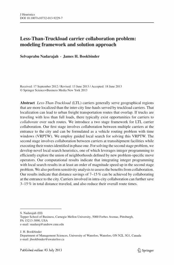
Collaboration is a strong relationship between multiple parties, with the goal ofa mutually beneficial outcome for all collaborating members. This paper focuseson operational collaboration (Sutherland 2006) between Less-Than-Truckload (LTL)transportation carriers. LTL carriers are concerned with delivery of small shipments(between 500 and 15,000 lbs on average) by truck to multiple consignees, ultimatelyover a limited geographical region. Figure 1 is a schematic showing the inter-cityline haul to the distribution network of the destination city and the subsequent localdeliveries. The distribution network includes distribution centers and vehicle depots,and is typically located away from the city center. Goods are received at this locationfrom their line haul journey and prepared for their local routes.

Shippers can also enter into operational collaboration, where they bundle lanesbefore their submission to a carrier. A lane is a contiguous portion of highway or road,considered by the carrier as a single link for routing purposes.

Carriers prefer bundled lanes, as they may lead to what are termed continuousmoves. Continuous Move Routes are ones in which we would ideally have zero dead-head miles and no asset-repositioning costs. The latter costs are incurred when atruck travels empty between two stops. This reduction in cost allows carriers to offermore competitive rates to the shipper, thereby providing an incentive for shippers tocollaborate.

The present paper deals with the specific problem of collaboration between LTLcarriers, whose loads are small in size and unpredictable. We consider the typical casewhere LTL carriers deliver loads within urban regions. In this setting, time windowsfor deliveries are usually tight. This leads to routes that are highly inefficient in termsof distance traveled, which our method aims to improve through collaboration.

We term the collaborative solution to the above stated problem as LTL col-laboration. LTL collaboration aims at designing efficient routes which minimize

Fig. 1 Line haul and localdelivery

123

Less-Than-Truckload carrier collaboration problem

asset-repositioning cost, total distance traveled, and maximizes truck asset utiliza-tion. Reduction in asset repositioning costs can lead to large savings for carriers, sincetrucks in the USA travel empty 20 % of the time on average (Wilson 2007). Localintra-city trucking costs were a staggering annual 435 billion United States dollars in2006 (Wilson 2007). The 2008 Canadian state of logistics report showed that truckingrepresented over 14 billion Canadian dollars, which was about 8 % of the Canadiangross domestic product (Industry Canada, 2008). These high costs also mean that smallimprovements through LTL collaboration will translate to large savings in real costsin both countries.

The main contributions of this paper are:

1. A two-stage framework for collaboration between LTL carriers. The first stageinvolves exchange of (partial) loads between carriers at the entry to the city, whiletrucks make such exchanges at transshipment points during local delivery in thesecond stage.

2. Novel heuristics that solve the mathematically complicated problem that resultsfrom the second stage of our collaborative framework. We develop a planningheuristic based on quadtree search to assist the decision maker in choosing trans-shipment points. For constructing collaborative routes using these transshipmentfacilities, we develop a local search heuristic based on new move operators andleverage integer programming to efficiently explore the union of the neighborhoodsdefined by these moves. Our computational tests indicate that our integration ofinteger programming with local search results in at least an order of magnitudespeed up when constructing collaborative routes.

3. Computational sensitivity analysis on a rectangular region with parameters cal-ibrated to the city of Toronto to assess the benefits to carriers from engaging incollaboration at the city entrance and in collaboration at transshipment points whileexecuting local routes. Our results indicate that collaboration at the city entranceresults in distance savings between 7–15 % over all carriers, and increases vehicleutilization by 4–5 %. Intra-city collaboration leads to route distance savings of3–15 % over collaborating carriers, and also reduces route times.

The remainder of this paper is organized as follows. We review the relevant liter-ature in Sect. 2. Definition of the carrier collaboration problem, and the hierarchicalframework for its study, are presented in Sect. 3. A high-level description of our solu-tion approach is given in Sect. 4; details of each heuristic are discussed in Sects.5–7. The evaluation procedure is described in Sect. 8, and computational results arepresented and discussed in Sect. 9. Concluding remarks and suggestions for futureresearch appear in Sect. 10.

2 Literature review

Carrier collaboration has received increased attention in recent years. A major part ofthis literature focuses on truckload collaboration; see Ergun et al. (2007), Liu et al.(2010), Özener et al. (2011) and references therein. There are also several referencesthat concern the allocation of profits from carrier collaboration among partners using

123


game theoretic methods. Examples include Houghtalen et al. (2011) and Özener et al.(2011).

Our emphasis in this article is rather on LTL collaboration, and Cruijssen andSalomon (2004), Krajewska and Kopfer (2006, 2009) are recent articles on this topic.Cruijssen and Salomon (2004) consider collaboration between multiple carriers, wherecollaboration involves the sharing of orders between transportation companies. Theyassess the benefit from collaboration by solving a capacitated vehicle routing problemfor each individual carrier (non-collaborative case) and compare this solution withthe solution from solving a single capacitated vehicle routing problem that combinesorders from all carriers (collaborative case). Krajewska and Kopfer (2006, 2009) alsostudy the problem of carriers sharing orders but they solve a pick up and deliveryproblem with time windows to determine when collaboration is beneficial. In additionto assessing the cost savings from collaboration, they use game theoretic mechanisms,namely core and Shapley value, to divide the savings among the coalition of carriers.A distinguishing feature of our work is the second stage of collaboration, collaborativerouting, which is absent in Cruijssen and Salomon (2004) and in Krajewska and Kopfer(2006, 2009). Thus we extend this literature in a significant manner, and our extensionprovides additional opportunities for LTL carriers to reduce travel distance and time.

The optimization problems that arise in our LTL collaboration framework are chal-lenging. Our first stage of collaboration at the entrance to the city involves solving avehicle routing problem with time windows (VRPTW). There is an extant literature onsolving VRPTW; see Bräysy and Gendreau (2005a,b) for a review of exact methodsand metaheuristics for its solution. We employ guided local search (GLS) (Voudourisand Tsang 1998, 2002) for solving our VRPTW in a manner similar to De Backer et al.(2000), and do not attempt to find a new approach here. Rather, our methodologicalcontributions are for the second stage of collaboration, which involves identifyingtransshipment opportunities between local routes of LTL carriers.

Instead of assuming that we have a set of predetermined transshipment points, weprovide a planning module that uses a quadtree search heuristic (Finkel and Bentley1974) to identify good transshipment points based on a flexible objective functionbecause we expect this decision to involve considerable human input. For identify-ing transshipment opportunities using these locations, we develop an integrated localsearch heuristic that leverages integer programming. Previous applications of inte-grated methods to solve challenging problems include Focacci et al. (1999), Jain andGrossmann (2001) and van Hoeve (2003). A more comprehensive list can be found inYunes (2012).

3 Problem description

Truck transportation of goods involves a line-haul leg and local routing (Fig. 1). Theline-haul journey of a truck is between cities, often a single origin and destination,while local delivery entails a multi-drop route. Inbound loads transported by severalcarriers arrive at the boundary of the city after a line haul from the respective origins.

The local routes that each carrier had originally intended to operate within thecity are referred to as “non-collaborative” routes. However, the carriers will be able

123


(a) (b)

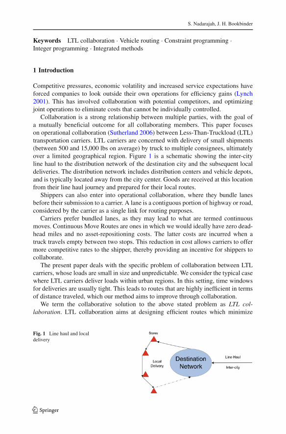
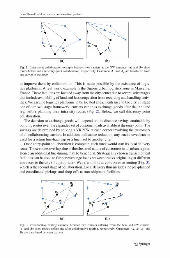
Fig. 2 Entry-point collaboration example between two carriers at the NW entrance. (a) and (b) showroutes before and after entry-point collaboration, respectively. Customers A1 and A2 are transferred fromone carrier to the other

to improve them by collaboration: This is made possible by the existence of logis-tics platforms. A real world example is the Sigoris urban logistics zone in Marseille,France. These facilities are located away from the city center due to several advantagesthat include availability of land and less congestion from receiving and handling activ-ities. We assume logistics platforms to be located at each entrance to the city. In stageone of our two-stage framework, carriers can thus exchange goods after the inboundleg, before planning their intra-city routes (Fig. 2). Below, we call this entry-pointcollaboration.

The decision to exchange goods will depend on the distance savings attainable bybuilding routes over the expanded set of customer loads available at the entry point. Thesavings are determined by solving a VRPTW at each corner involving the customersof all collaborating carriers. In addition to distance reduction, any trucks saved can beused for a return line-haul trip or a line haul to another city.

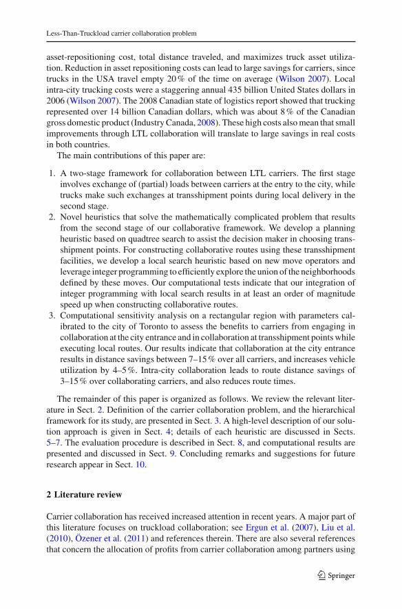
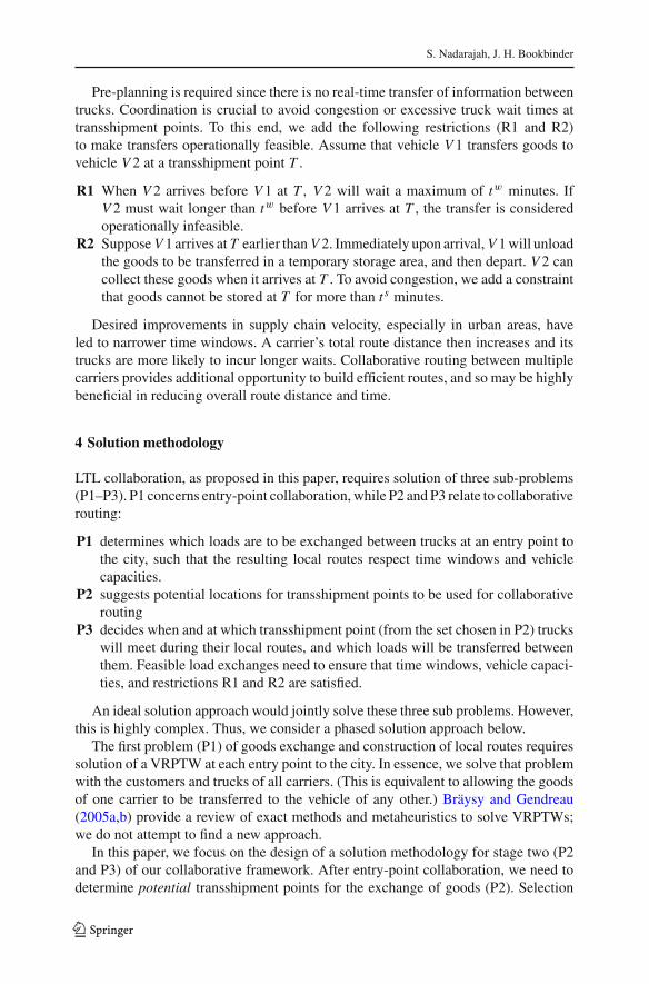
Once entry-point collaboration is complete, each truck would start its local deliveryroute. Those routes overlap, due to the clustered nature of customers in an urban region.Hence an additional fine-tuning may be beneficial. Strategically chosen transshipmentfacilities can be used to further exchange loads between trucks originating at differententrances to the city (if appropriate). We refer to this as collaborative routing (Fig. 3),which is the second stage of collaboration. Local delivery thus includes the pre-plannedand coordinated pickups and drop-offs at transshipment facilities.

(a) (b)

Fig. 3 Collaborative routing example between two carriers entering from the NW and SW corners.(a) and (b) show routes before and after collaborative routing, respectively. Customers A1, A2, B1 andB2 are transferred between carriers

123


Pre-planning is required since there is no real-time transfer of information betweentrucks. Coordination is crucial to avoid congestion or excessive truck wait times attransshipment points. To this end, we add the following restrictions (R1 and R2)to make transfers operationally feasible. Assume that vehicle V 1 transfers goods tovehicle V 2 at a transshipment point T .

R1 When V 2 arrives before V 1 at T, V 2 will wait a maximum of tw minutes. IfV 2 must wait longer than tw before V 1 arrives at T , the transfer is consideredoperationally infeasible.

R2 Suppose V 1 arrives at T earlier than V 2. Immediately upon arrival, V 1 will unloadthe goods to be transferred in a temporary storage area, and then depart. V 2 cancollect these goods when it arrives at T . To avoid congestion, we add a constraintthat goods cannot be stored at T for more than t s minutes.

Desired improvements in supply chain velocity, especially in urban areas, haveled to narrower time windows. A carrier’s total route distance then increases and itstrucks are more likely to incur longer waits. Collaborative routing between multiplecarriers provides additional opportunity to build efficient routes, and so may be highlybeneficial in reducing overall route distance and time.

4 Solution methodology

LTL collaboration, as proposed in this paper, requires solution of three sub-problems(P1–P3). P1 concerns entry-point collaboration, while P2 and P3 relate to collaborativerouting:

P1 determines which loads are to be exchanged between trucks at an entry point tothe city, such that the resulting local routes respect time windows and vehiclecapacities.

P2 suggests potential locations for transshipment points to be used for collaborativerouting

P3 decides when and at which transshipment point (from the set chosen in P2) truckswill meet during their local routes, and which loads will be transferred betweenthem. Feasible load exchanges need to ensure that time windows, vehicle capaci-ties, and restrictions R1 and R2 are satisfied.

An ideal solution approach would jointly solve these three sub problems. However,this is highly complex. Thus, we consider a phased solution approach below.

The first problem (P1) of goods exchange and construction of local routes requiressolution of a VRPTW at each entry point to the city. In essence, we solve that problemwith the customers and trucks of all carriers. (This is equivalent to allowing the goodsof one carrier to be transferred to the vehicle of any other.) Bräysy and Gendreau(2005a,b) provide a review of exact methods and metaheuristics to solve VRPTWs;we do not attempt to find a new approach.

In this paper, we focus on the design of a solution methodology for stage two (P2and P3) of our collaborative framework. After entry-point collaboration, we need todetermine potential transshipment points for the exchange of goods (P2). Selection

123


of good transshipment points will depend on the particular routes to be executed bydifferent carriers. The routes themselves change on an operational basis, possibly fromone day to another. Therefore, the use of dedicated facilities may not be practical.

Crainic et al. (2008) propose that city bus terminals and tour bus parking lots beused as transshipment points. Although their two-level logistics system has a differentproblem setting than ours, this suggests that we need to identify which existing setof facilities will be most suited for collaborative routing, rather than locating newones. The actual benefit of a transshipment point, however, can only be measured aftersolving the collaborative routing problem. Therefore, we have designed a flexible plan-ning module to guide the decision maker in locating or choosing potentially beneficialtransshipment points. Our module suggests good transshipment point locations, whichcan then be changed by the user.

Finally, once transshipment points are decided, we construct collaborative routes(P3) via an integrated method which uses an integer programming model within localsearch. We refer to P1–P3 together as the Collaborative Vehicle Routing Problem withTime Windows (COLL-VRPTW). In the remaining sections, we discuss each phasein the proposed three-phase solution procedure.

5 Phase 1: entry-point collaboration

Phase one employs a guided local search (GLS) method to solve the VRPTWs encoun-tered in entry-point collaboration. In guided local search (Voudouris and Tsang 1998,2002), a rather recent addition as a metaheuristic, the objective function is modifiedto direct the search. This is done by defining a set of features for a problem and penal-izing a subset of those features. The selection of features is done such that the searchpromotes candidate solutions with “good features,” where a good feature is one whichoccurs often at a local optimum. Only the weight of the penalty term (i.e. a singleparameter) in the objective function needs to be tuned in GLS, an added advantage.Voudouris and Tsang (2002) contain further details.

To solve the VRPTW, we utilize a GLS that is very similar to the one used in DeBacker et al. (2000). A constraint programming engine aids the given local searchmethod by acting as a “rule-checker.” Each constraint is propagated via specializedalgorithms (Rossi et al. 2007), to reduce the search space; the overall performanceof GLS depends on the effectiveness of constraint propagation. Therefore, this is anintegration of heuristics and constraint programming (Hooker 2007).

We employ the GLS template in ILOG Dispatcher 4.6 which is based upon ILOGSolver 6.6. ILOG Dispatcher is a flexible system built on top of the constraint pro-gramming engine in ILOG Solver for solution of complex vehicle routing problemswith side constraints. Our implementation of the GLS uses Cross, Exchange, Relo-cate, Or-opt and 3-Opt moves to define the search neighborhood. These operators arediscussed in detail by Kindervater and Savelsbergh (2003).

6 Phase 2: transshipment point location

Broadly, phase 2 involves steps or considerations a, b and c, whose details will follow:

123


a. Clusters of customers are formed; a quadtree search applies a heuristic functionto evaluate the potential clusters. Jain et al. (1999) provide a survey of variousclustering methods.)

b. Given the clusters, a centroid method will decide the location of transshipmentpoints.

c. Sensitivity analysis or fine tuning. The quadtree search enables easy changes tothe heuristic function, making it possible to incorporate other subjective criteriain forming clusters and evaluating transshipment sites.

The goal of this phase is to use a heuristic function to recommend potential sitesfor transshipment points. The user would choose the suggested location if it coincideswith an actual transhipment point, or change it to the closest one.

Given a COLL-VRPTW instance, the second phase of our algorithmic frameworkthus applies an adaptive quadtree search (Finkel and Bentley 1974) to create clustersof customers. At a high level, in a quadtree (also known as a region quadtree), a two-dimensional space is recursively decomposed into four smaller quadrants, startingfrom a bounding rectangle, until some termination criterion is met. Therefore, eachinternal parent node has four children. An evaluation function is used to score eachnode in a quadtree and pick a subset of nodes based on these scores.

In more detail, our quadtree search implementation in Java takes as inputs an array ofevaluation function parameters −→α , the number Np of transshipment points or clustersto be returned, the minimum area Amin of a cluster, the minimum number Cmin ofcustomer points in a cluster, and the coordinate set [X, Y ] whose elements are thex and y coordinates of all customers. The array −→α contains the weights associatedwith each term in the evaluation function. We always employ a convex combination∑

i αi = 1, in which the weights αi can be varied to reflect the importance of differentterms.

Once the input values are given, customer coordinates and other characteristicssuch as demand and time windows are read. Using spatial coordinates of customers, abounding rectangle which encloses all the points is initialized and assigned to the rootof the quadtree. Entry points are assumed to be located at the vertices of that rectangle.

The quadtree is recursively built starting at the bounding rectangle. A quadrant isstored at every node in the quadtree and a unique “position” is used to retrieve it.When that is completed, we use the evaluation function specified by the −→α vectorto score each quadrant. The Np non-overlapping clusters with the highest scores arethen selected. Finally, transshipment points are located in these chosen clusters usingeither a demand-weighted or time window slack weighted centroid. These choices aremotivated by the potential desire to have transhipment points close to (i) important (i.e.,high demand) customers or (ii) locations that are closer to customers with larger time-window slack so that the potential of finding a time-window feasible transshipment ishigher. We discuss details of the evaluation and transshipment location functions inSect. 9.2.

By associating a transshipment point with a cluster of customers, we inherentlyapply a radius function to limit the set of customers considered during collaborativerouting. The preceding approach has similarities to Taillard (1993) where a largerrouting problem is partitioned into smaller sub-problems before applying local search.

123


The partitioning of the parent into children takes time O(n p), where n p is thenumber of points in quadrant p, and is the most costly operation in building a quadtree.The termination criteria involve Amin and Cmin . It can be shown that the quadtree hasO((d + 1)nmax ) nodes and can be constructed in a time O((d + 1)n), where d is the

depth of the quadtree, nmax =⌈

n

Cmin

⌉

and n is the number of customers or points

within the initial bounding rectangle. Further, it can be shown that d is bounded by3

2+ min

[

log2

(l

b

)

, 1 + log4

(AB

Amin

)]

, where l, b and AB are the length, breadth

and area of the initial bounding rectangle.

7 Phase 3: collaborative routing

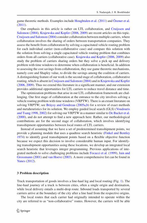
Our final algorithm is an integrated greedy local search method. Given routes fromPhase 1 and clusters and transshipment points from Phase 2, we search for collabo-rative routing opportunities between trucks entering at different entrances to the city.We define three new transshipment-specific move operators (SM1–SM3) for neigh-borhood definition. These move operators transfer a sequence of customers from oneroute to another, by exchanging goods at a transshipment point. Each move operatoralso defines an exclusive neighborhood, i.e. the neighborhoods of the SMi are pair-wise disjoint. The transferred sequence is inserted between successive customers onthe route being given the loads. We refer to the truck receiving an increase in its load asa load taker; the vehicle whose load is reduced is a load giver. (These will respectivelybe abbreviated below as LT and LG.)

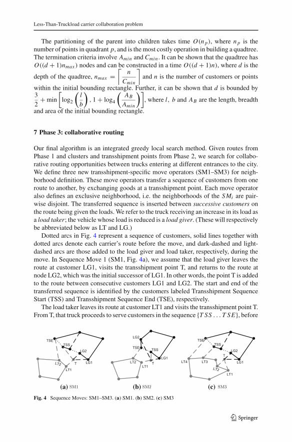
Dotted arcs in Fig. 4 represent a sequence of customers, solid lines together withdotted arcs denote each carrier’s route before the move, and dark-dashed and light-dashed arcs are those added to the load giver and load taker, respectively, during themove. In Sequence Move 1 (SM1, Fig. 4a), we assume that the load giver leaves theroute at customer LG1, visits the transshipment point T, and returns to the route atnode LG2, which was the initial successor of LG1. In other words, the point T is addedto the route between consecutive customers LG1 and LG2. The start and end of thetransferred sequence is identified by the customers labeled Transshipment SequenceStart (TSS) and Transshipment Sequence End (TSE), respectively.

The load taker leaves its route at customer LT1 and visits the transshipment point T.From T, that truck proceeds to serve customers in the sequence {T SS . . . T SE}, before

(a) (b) (c)

Fig. 4 Sequence Moves: SM1–SM3. (a) SM1. (b) SM2. (c) SM3

123


returning to its route at LT2. Therefore, the nodes T⋃{T SS . . . T SE} are inserted

between consecutive customers LT1 and LT2.In Sequence Move 2 (SM2 of Fig. 4b), the load taker’s operations are identical to

those of SM1, but now the transferred sequence is removed from between LG1 andLG2. Therefore, distinct from SM1, LG1 and LG2 are not successive customers.

In SM1 and SM2, the load taker visits TSS immediately following the transshipmentpoint. Sequence Move 3 (SM3) considers the situation where the load taker returns tothe route at LT2 after receiving loads corresponding to those in the transferred sequence{T SS . . . T SE} but before actually serving those customers (Fig. 4c). To deliver theloads collected at T the load taker deviates from the route at LT3 (a customer appearinglater in the route) and serves the customers {T SS . . . T SE} before returning to its ownroute at LT4.

SM3 is thus the most complicated move, as additional decisions regarding LT3 andLT4 have to be made. Note also that each of the preceding moves SMi , i = 1, 2, 3,preserves the direction of the transferred sequence.

Let T be the set of transshipment points returned by the quadtree search method, andClusterT , the set of customers in the cluster associated with transshipment point T ∈T. A “transshipment opportunity” is one where two trucks can meet at a transshipmentpoint and transfer loads. The following is then a high-level, step-wise explanation ofthe collaborative routing algorithm which is used to find transshipment opportunities.

1. Set iteration count: i = 0.2. For each transshipment point T ∈ T, propagate time window constraints for all

customers in the cluster. This is done by keeping a feasibility record for eachcustomer c ∈ ClusterT for all T ∈ T. That is, we check whether the addition ofT in between c and its predecessor, or between c and its successor, satisfies thetime window constraints. c is removed from ClusterT if neither of the precedinginsertion cases is feasible.

3. Search the non-tabu neighborhood defined by SM1–SM3 using a heuristic spec-ified by the parameter type. Based on the value of type, one of the following isreturned as the set of feasible transshipment opportunities (FT Oi ): (a) The firstopportunity in the neighborhood; (b) the best opportunity, or (c) the set of oppor-tunities that maximize savings.

4. Update the routes for each to ∈ FT Oi . This is when we actually make the moveto a new solution.

5. Remove customers in each to ∈ FT Oi from their respective clusters.6. If |FT Oi | > 0, set i = i + 1 and return to Step 3. Otherwise, end.

The above template searches for feasible transshipment opportunities by fully specify-ing a transhipment-specific move SM1 or SM2 or SM3 with positive distance savings.This specification includes the choice of customer pairs (LT1, LT2) and (LG1, LG2).We use customers in ClusterT as candidates for LT1, LT2, LG1 and LG2. Step 2removes customers in ClusterT if time window constraints are violated when insert-ing T . This is justified because SM1–SM3 insert T in between (LT1, LT2) and (LG1,LG2). In Step 5, we remove all customers that are already part of a transshipmentopportunity so that moves are created using other customers in the cluster.

123


7.1 Greedy set search

If the parameter type is equal to greedy set, we employ an optimization module whichworks as follows. Assume that we are currently at a solution s. We define a feasibletransshipment opportunity to be a move from s to a new feasible solution, when thatalso results in distance savings and preserves feasibility (i.e. it represents an improvingfeasible move). Feasibility includes time windows, vehicle capacity and restrictionsR1 and R2. We define T Os to be the set of all feasible transshipment opportunitiesthat can be reached from s by applying one of the move operators. Each element inthis set will contain the information required to make the changes and move to thenew feasible solution it represents.

When searching for the best improving feasible move, we naturally must explorethe neighborhood of a solution (or a subset of that neighborhood), before declaring thissolution to be the best. During exploration, we encounter many improving feasiblemoves that eventually might not be used. In the greedy set case, we now combinethose opportunities to more efficiently benefit from the information gathered duringneighborhood exploration.

The preceding combination of moves is performed by an integer programmingmodel that greedily selects the savings-maximizing subset of moves that, when usedon the current solution, will lead to a feasible solution. We refer to this combination offeasible moves as a “super move.” In each iteration, SM1, SM2 or SM3 applied alonewill result in a transfer of customers from one route to another. Examples of supermoves include the exchange of customers between routes, or when a route acts as botha load giver and a load taker, or that route acts as a load giver to two load takers.

Understandably, only some combinations of moves are feasible. We thus add con-straints to the integer programming model to ensure that only feasible combinationsare considered. These constraints are based mainly on Propositions 6.1 and 6.2, whereT OT denotes the set of feasible transshipment opportunities at T .

Proposition 7.1 Let to1, to2 ∈ T OT have the same load-giver route but differentload-taker routes. Suppose that the customer LG1 at which the load giver leaves theroute is the same for to1 and to2, and the transferred sequences have no customers incommon. Then to1 and to2 can be combined to form a feasible super move.

Proof Since to1 and to2 involve different load taker routes, combining them will notchange the load received by each load taker. Since to1 and to2 are capacity-feasibleby definition, the super move is also capacity feasible.

If to1 and to2 have the same LG1 (Fig. 4), then the arrival times of the load giverat T will be identical in both cases. The removal of customers from the load giverby using to1 and to2 occurs after T . As a result, the arrival time of the load giver atT does not change. This preserves the load taker’s time window feasibility and alsoensures transshipment feasibility (i.e. satisfaction of R1 and R2) at T .

Combining to1 and to2 is equivalent to using the opportunities sequentially in anyorder. Suppose to2 is used following to1. This amounts to removing customers trans-ferred in to2, in addition to the customer sequence transferred in to1. The transferredsequence in both to1 and to2 contains customers visited after the transshipment point,and each sequence is unique as we ensure sequences do not overlap. to1 is feasible

123


by definition, and removing more customers by using to2 after to1 preserves the loadgiver’s time window feasibility. The same holds true if to1 is applied following to2.

��Proposition 7.2 Suppose to1, to2 ∈ T OT where the load-taker route of to1 is thesame as the load-giver route of to2. If the respective customers, C1lt

to1and C1lg

to2, at

which the load taker and load giver leave the route are the same, then to1 and to2 canbe feasibly combined.

Proof When to1 and to2 are combined, the load giver of to1 remains feasible as it isnot affected by to2. Let V 1 refer to the vehicle corresponding to the route commonto to1 and to2, and V 2 denote the vehicle of the load giver in to1. If C1lt

to1= C1lg

to2,

the arrival time of V 1 at transshipment point T will be identical for both to1 and to2.Hence the transshipment feasibility is preserved.

Let C2ltto1

and C2lgto2

denote the customers at which V 1 returns back to its route into1 and to2, respectively, after visiting T . Regardless of the move type, V 1 returnsto its original route at point C2lt

to1in to1. By definition, this move is feasible. If to2

is of type SM1 or SM3, then C2ltto1

= C2lgto2

. Using to2 corresponds to removing

customers from V 1’s route after C2lgto2

. Therefore, time window feasibility of V 1 ispreserved by combining to1 and to2. When to2 is defined by SM2, the combination isequivalent to applying to1 followed by to2. to1 results in the addition of new customersbetween C1lt

to1and C2lt

to1. This is feasible by definition. If we now apply to2, it will

remove customers starting from C2ltto1

. Therefore, the time window feasibility of V 1is preserved.

Let Atv1T and Atv2

T denote the arrival times of V 1 and V 2 at T , respectively. Into1, if Atv2

T > Atv1T (i.e. restriction R1), V 1 will have to wait before starting service

at T . As a result, the departure time, Dtv1T of V 1 at T in to1 may be greater than

Atv1T + sT , where sT is the service time at T . However, as a load giver in to2, V 1 can

start off-loading the goods it will be transferring out upon immediate arrival at T (i.e.at Atv1

T ), regardless of whether Atv2T > Atv1

T . Since time window feasibility of theload taker in to2 depends only on the service start time of V 1 at T , the combination isfeasible. When Atv2

T ≤ Atv1T , the route corresponding to V 1 is clearly time window

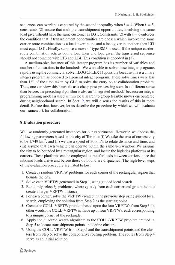
feasible. ��Definitions of the sets used in the integer programming model are given in Table

2, while the model itself is contained in Table 1. T O is the set of all transshipmentopportunities, i.e.

⋃

TT OT . Savto is the distance savings if transshipment opportunity

to ∈ T O is used. Rltto and Rlg

to are the routes associated with the load taker and loadgiver, respectively, of to.

The “rank of a customer” is the index (position in sequence) of that customer onits route, starting with the depot as zero. The ranks of customers LT3 and LT4 in theroute are given by rC3lt

to and rC4ltto. C1lt

to and C1lgto are LG1 and LT1 associated with

to. The type of move (i.e. SM1, SM2 or SM3) associated with to is denoted as I Dto.Each transferred sequence in to has associated with it the rank of TSS, r Sto and therank of TSE, r Eto. P is the set of unique load takers. For a given load taker p ∈ Pwe denote its associated route by Rp.

123


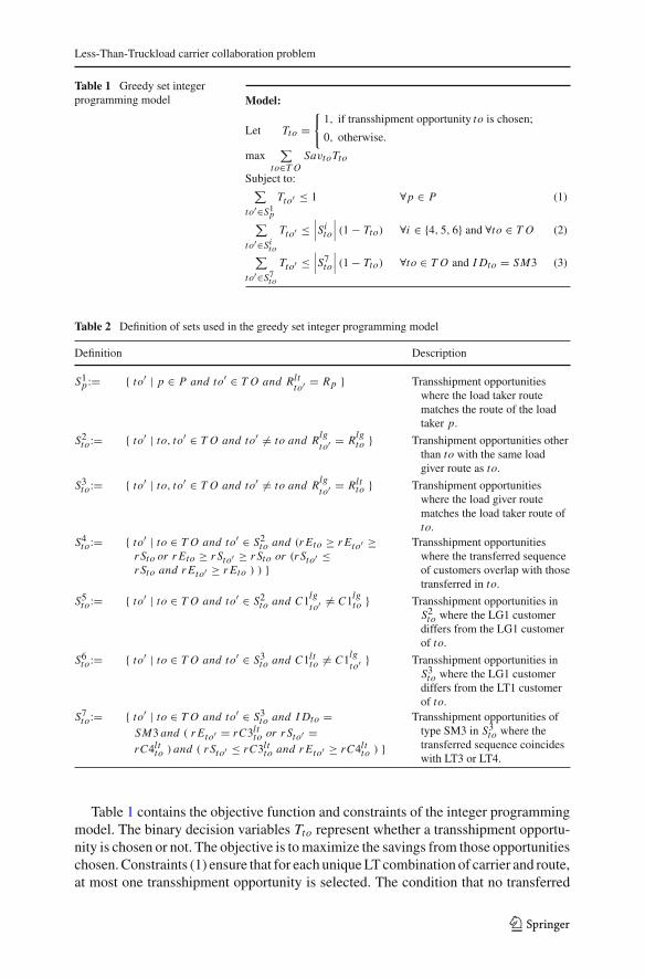
Table 1 Greedy set integerprogramming model Model:

Let Tto ={

1, if transshipment opportunity to is chosen;

0, otherwise.

max∑

to∈T OSavtoTto

Subject to:∑

to′∈S1p

Tto′ ≤ 1 ∀p ∈ P (1)

∑

to′∈Sito

Tto′ ≤∣∣∣Si

to

∣∣∣ (1 − Tto) ∀i ∈ {4, 5, 6} and ∀to ∈ T O (2)

∑

to′∈S7to

Tto′ ≤∣∣∣S7

to

∣∣∣ (1 − Tto) ∀to ∈ T O and I Dto = SM3 (3)

Table 2 Definition of sets used in the greedy set integer programming model

Definition Description

S1p := { to′ | p ∈ P and to′ ∈ T O and Rlt

to′ = Rp } Transshipment opportunitieswhere the load taker routematches the route of the loadtaker p.

S2to:= { to′ | to, to′ ∈ T O and to′ = to and Rlg

to′ = Rlgto } Transhipment opportunities other

than to with the same loadgiver route as to.

S3to:= { to′ | to, to′ ∈ T O and to′ = to and Rlg

to′ = Rltto } Transhipment opportunities

where the load giver routematches the load taker route ofto.

S4to:= { to′ | to ∈ T O and to′ ∈ S2

to and (r Eto ≥ r Eto′ ≥r Sto or r Eto ≥ r Sto′ ≥ r Sto or (r Sto′ ≤r Sto and r Eto′ ≥ r Eto ) ) }

Transshipment opportunitieswhere the transferred sequenceof customers overlap with thosetransferred in to.


to and C1lgto′ = C1lg

to } Transshipment opportunities inS2

to where the LG1 customerdiffers from the LG1 customerof to.


to and C1ltto = C1lg

to′ } Transshipment opportunities inS3

to where the LG1 customerdiffers from the LT1 customerof to.


to and I Dto =SM3 and ( r Eto′ = rC3lt

to or r Sto′ =rC4lt

to ) and ( r Sto′ ≤ rC3ltto and r Eto′ ≥ rC4lt

to ) }

Transshipment opportunities oftype SM3 in S3

to where thetransferred sequence coincideswith LT3 or LT4.

Table 1 contains the objective function and constraints of the integer programmingmodel. The binary decision variables Tto represent whether a transshipment opportu-nity is chosen or not. The objective is to maximize the savings from those opportunitieschosen. Constraints (1) ensure that for each unique LT combination of carrier and route,at most one transshipment opportunity is selected. The condition that no transferred

123


sequences can overlap is captured by the second inequality when i = 4. When i = 5,constraints (2) ensure that multiple transshipment opportunities, involving the sameload giver, should have the same customer as LG1. Constraints (2) with i = 6 enforcesthe condition that if transshipment opportunities are chosen which involve the samecarrier-route combination as a load taker in one and a load giver in another, then LT1must equal LG1. Finally, suppose a move of type SM3 is used. If the unique carrier-route combination acts as both a load taker and load giver, the transferred sequenceshould not coincide with LT3 and LT4. This condition is encoded in (3).

A medium-size instance of this integer program has its number of variables andnumber of constraints in the hundreds. We were able to solve these integer programsrapidly using the commercial solver ILOG CPLEX 11, possibly because this is a binaryinteger program as opposed to a general integer program. These solve times were lessthan 1 % of the time taken by GLS to solve the entry point collaboration problem.Thus, one can view this heuristic as a cheap post-processing step. In a different sensethan before, the preceding algorithm is also an “integrated method,” because an integerprogramming model is used within local search to group feasible moves encounteredduring neighborhood search. In Sect. 9, we will discuss the results of this in moredetail. Before that, however, let us describe the procedure by which we will evaluateour framework for collaboration.

8 Evaluation procedure

We use randomly generated instances for our experiments. However, we choose thefollowing parameters based on the city of Toronto: (i) We take the area of our test cityto be 1,749 km2, and (ii) we use a speed of 30 km/h to relate distance and time, and(iii) assume that each vehicle can operate within the same 8-h window. We assumethe city to be bounded by a rectangular region, and locate the logistics platforms at itscorners. These platforms can be employed to transfer loads between carriers, once theinbound loads arrive and before those outbound are dispatched. The high-level stepsof the evaluation procedure are listed below:

1. Create l1 random VRPTW problems for each corner of the rectangular region thatbounds the city.

2. Solve each VRPTW generated in Step 1, using guided local search.3. Randomly select l2 problems, where l2 < l1 from each corner and group them to

create a larger VRPTW instance.4. For each corner, solve the VRPTW created in the previous step using guided local

search, employing the solution from Step 2 as the starting point.5. Create the COLL-VRPTW problem based upon the four VRPTWs from Step 3. In

other words, the COLL-VRPTW is made up of four VRPTWs, each correspondingto a unique corner of the rectangle.

6. Apply the quadtree search algorithm to the COLL-VRPTW problem created inStep 5 to locate transshipment points and define clusters.

7. Using the COLL-VRPTW from Step 5 and the transshipment points and the clus-ters from Step 6, solve the collaborative routing problem. The routes from Step 4serve as an initial solution.

123


The l1 VRPTWs in Step 1 are randomly generated by modifying the procedurefound in Solomon (1987). We set l1 equal to 10 (i.e. we generate 10 random VRPTWsfor each corner). These problems are generated by fixing a set of input parameters. LetPi represent an input-characterizing parameter, where i ∈ K , and K is the set of allinput parameters. Further, let Di = {di

j1, . . . , di

jn} represent the domain of Pi . Then a

setting s ∈ S is defined as the combination [ps1, . . . , ps

K ] where psi ∈ Di is the value

taken by input parameter Pi .In our analysis, a setting is characterized by the following parameters and domains:

The number of customers n ∈ {25, 50, 75, 150, 300} in each of the l1 problems createdin Step 1, the ratio of length (l) to breadth (b) of the urban region (l/b ∈ {1, 1.5, 2}),percentage of customers with time windows (T W ∈ {75, 100}), and the mean widthw of the time window, w ∈ {1, 2}, in hours.

Across instances, we assume that the vehicle capacity is 42,000 lbs which is the stan-dard weight limit of a 40-foot container. Customer demands are generated uniformlywithin the interval [500 15,000], which is the typical load range for LTL shipments.

The l2 carriers that are randomly grouped in Step 3 are assumed to be those thatcollaborate. Following experimentation with l2 = 2 and 3, we chose an l2 value of4 for our computations. The resulting larger VRPTW will have a customer set thatincludes customers from the four collaborating carriers and their combined fleet ofvehicles. The number of customers in this larger VRPTW is denoted by N , whereN = 4n. In Step 4, we solve the VRPTW to obtain the new local delivery routes withcollaboration at the entrance to the city.

Step 6 applies the quadtree search algorithm to the COLL-VRPTW problem tocreate clusters of customers and then locate transshipment facilities. The number ofcustomers in the COLL-VRPTW is denoted by Nc, where Nc = 4N . Finally Step7 uses the transshipment points and the routes after entry-point collaboration to findcollaborative routing opportunities.

Sometimes in the literature, papers which solve multiple random instances reportonly the mean of their computational results. This can be misleading: If the corre-sponding distribution has a large dispersion, the sample mean may be a poor estimateof the desired population mean. We overcome that problem as follows. Since l2 < l1,one iteration of Steps 3–7 produces one sample point for a given setting. Repeatingthis multiple times allows us to construct a mean and a confidence interval for thatsetting. We develop 90 % confidence intervals using a t-distribution.

9 Results

In this section, we present and discuss results for each phase of our heuristic. Theevaluation procedure of Sect. 8 was used for all results reported here. We solved a totalof about 1,000 VRPTWs for entry-point collaboration, and close to 500 collaborativerouting problems. All our computations were performed on a 3Ghz Pentium 4 machinewith 1Gb of RAM. For each metric (e.g. distance saved), we report the mean (μ), the90 % confidence interval using the lower (le) and upper ends (ue) of the interval, andthe half-width (hw) of the confidence interval.

Note that we make two types of statistical comparisons. For a given vector of set-tings, and for each metric, “collaboration” is a statistically significant improvement

123


over “no collaboration” (10 % level of significance). That is, the corresponding 90 %confidence intervals, for the difference in performance, do not include zero: Collabo-ration out-performs no collaboration (in a statistically significant way) in the case ofevery metric.

The second type of comparison concerns two different settings, for the same policy.For example, when the percentage of customers with time windows is changed from75 to 100 %; what is the effect upon collaboration? A statement that distance savings(or another metric) of setting 2 is greater than setting 1 implies that the lower and upperends of setting 2’s confidence interval were greater than the lower and upper ends ofsetting 1’s confidence interval, respectively. (Such a statement may not be statisticallysignificant, but it does show a trend in the effect of a parameter.) Incidentally, whenwe say the distance saved (or any other statistic) increases with changes in a parameterPi , i ∈ K , it is assumed that all other parameters (i.e. Pj , j ∈ K and j = i) are fixed.

We use GLS with the objective of minimizing route distance to solve VRPTWs. Wealso implemented a tabu search method with probabilistic diversification to compareto the effectiveness of GLS. As a benchmark, we used the well known instances ofSolomon (1987). The data sets there are made up of six classes: C1, C2, R1, R2, RC1and RC2. Each problem has 100 customers. The C problems have clustered customersand are relatively easy to solve. The R problems are randomly generated and have noinherent spatial structure. The RC problems are a mixture of random and clusteredcustomers. Further, C1, R1 and RC1 are short horizon problems. Those solutionsrequire more vehicles, and the number of customers per route is small. In contrast,problem sets C2, R2 and RC2 have a long horizon and require fewer vehicles. We usedC1, R2 and RC1 as our training set, and C2, R1 and RC2 as the test set. Our designgoal was to obtain high quality results very quickly, as some of the random data setswe generate are larger than those of Solomon (1987).

A number of times, the GLS solution was equal to the best known solution for agiven problem in Solomon (1987). Although Tabu Search was better than GLS on afew problems, the results were always close. Moreover, far less time was required totune GLS than tabu search, and since we used a probabilistic tabu search, GLS had theadvantage of being deterministic. As a result, we used GLS for all results presentedhere.

In GLS, the weight λ of the penalty term in the objective function is the onlyparameter that needs to be tuned. For VRPTW of size less than one hundred customers,the best value of λ varied, but for larger problems (i.e. the randomly generated datasets), a value of 0.2 gave the best average case performance. Therefore, λ = 0.2 wasused for all the numerical results that we report.

9.1 Entry-point collaboration

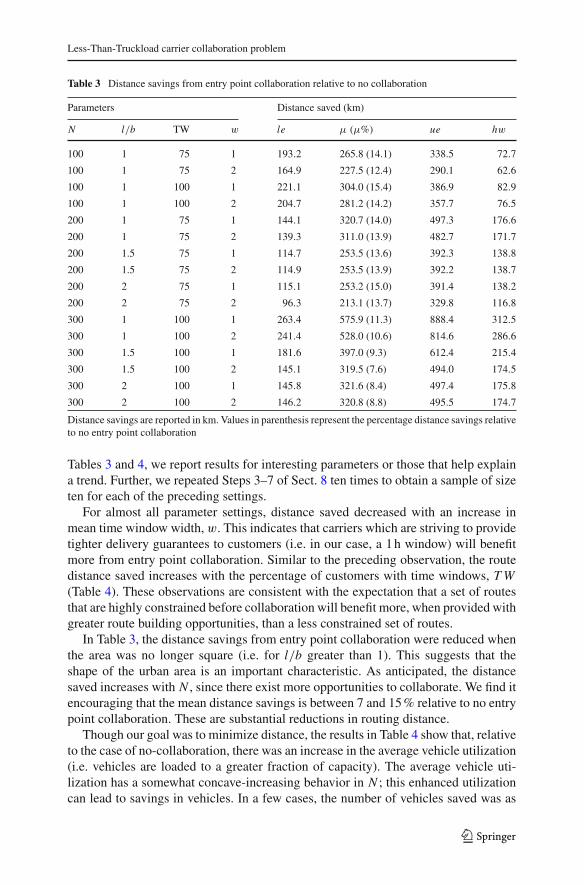
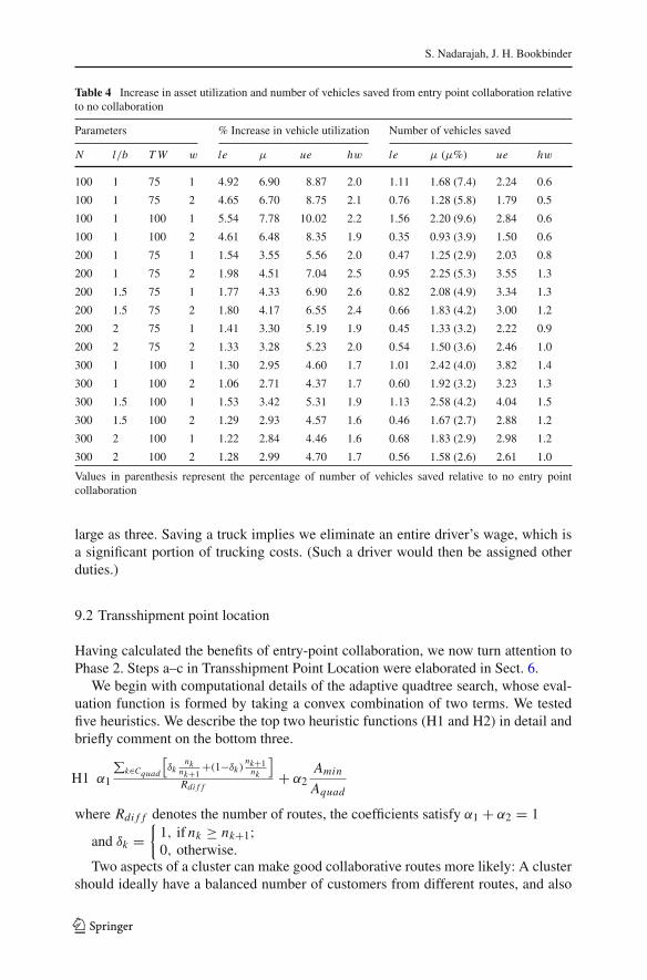
Table 3 reports confidence intervals for the distance saved and the percentage distancesaved relative to no collaboration. Table 4 reports the average increase in vehicle utiliza-tion, the number of vehicles saved from entry-point collaboration, and the percentageof vehicles saved relative to no collaboration. For N ∈ {100, 200, 300}, computationswere done for all possible settings (i.e. combinations of parameters [p1, . . . , pK ]). In

123


Table 3 Distance savings from entry point collaboration relative to no collaboration

Parameters Distance saved (km)

N l/b TW w le μ (μ%) ue hw

100 1 75 1 193.2 265.8 (14.1) 338.5 72.7

100 1 75 2 164.9 227.5 (12.4) 290.1 62.6

100 1 100 1 221.1 304.0 (15.4) 386.9 82.9

100 1 100 2 204.7 281.2 (14.2) 357.7 76.5

200 1 75 1 144.1 320.7 (14.0) 497.3 176.6

200 1 75 2 139.3 311.0 (13.9) 482.7 171.7

200 1.5 75 1 114.7 253.5 (13.6) 392.3 138.8

200 1.5 75 2 114.9 253.5 (13.9) 392.2 138.7

200 2 75 1 115.1 253.2 (15.0) 391.4 138.2

200 2 75 2 96.3 213.1 (13.7) 329.8 116.8

300 1 100 1 263.4 575.9 (11.3) 888.4 312.5

300 1 100 2 241.4 528.0 (10.6) 814.6 286.6

300 1.5 100 1 181.6 397.0 (9.3) 612.4 215.4

300 1.5 100 2 145.1 319.5 (7.6) 494.0 174.5

300 2 100 1 145.8 321.6 (8.4) 497.4 175.8

300 2 100 2 146.2 320.8 (8.8) 495.5 174.7

Distance savings are reported in km. Values in parenthesis represent the percentage distance savings relativeto no entry point collaboration

Tables 3 and 4, we report results for interesting parameters or those that help explaina trend. Further, we repeated Steps 3–7 of Sect. 8 ten times to obtain a sample of sizeten for each of the preceding settings.

For almost all parameter settings, distance saved decreased with an increase inmean time window width, w. This indicates that carriers which are striving to providetighter delivery guarantees to customers (i.e. in our case, a 1 h window) will benefitmore from entry point collaboration. Similar to the preceding observation, the routedistance saved increases with the percentage of customers with time windows, T W(Table 4). These observations are consistent with the expectation that a set of routesthat are highly constrained before collaboration will benefit more, when provided withgreater route building opportunities, than a less constrained set of routes.

In Table 3, the distance savings from entry point collaboration were reduced whenthe area was no longer square (i.e. for l/b greater than 1). This suggests that theshape of the urban area is an important characteristic. As anticipated, the distancesaved increases with N , since there exist more opportunities to collaborate. We find itencouraging that the mean distance savings is between 7 and 15 % relative to no entrypoint collaboration. These are substantial reductions in routing distance.

Though our goal was to minimize distance, the results in Table 4 show that, relativeto the case of no-collaboration, there was an increase in the average vehicle utilization(i.e. vehicles are loaded to a greater fraction of capacity). The average vehicle uti-lization has a somewhat concave-increasing behavior in N ; this enhanced utilizationcan lead to savings in vehicles. In a few cases, the number of vehicles saved was as

123


Table 4 Increase in asset utilization and number of vehicles saved from entry point collaboration relativeto no collaboration

Parameters % Increase in vehicle utilization Number of vehicles saved

N l/b T W w le μ ue hw le μ (μ%) ue hw

100 1 75 1 4.92 6.90 8.87 2.0 1.11 1.68 (7.4) 2.24 0.6

100 1 75 2 4.65 6.70 8.75 2.1 0.76 1.28 (5.8) 1.79 0.5

100 1 100 1 5.54 7.78 10.02 2.2 1.56 2.20 (9.6) 2.84 0.6

100 1 100 2 4.61 6.48 8.35 1.9 0.35 0.93 (3.9) 1.50 0.6

200 1 75 1 1.54 3.55 5.56 2.0 0.47 1.25 (2.9) 2.03 0.8

200 1 75 2 1.98 4.51 7.04 2.5 0.95 2.25 (5.3) 3.55 1.3

200 1.5 75 1 1.77 4.33 6.90 2.6 0.82 2.08 (4.9) 3.34 1.3

200 1.5 75 2 1.80 4.17 6.55 2.4 0.66 1.83 (4.2) 3.00 1.2

200 2 75 1 1.41 3.30 5.19 1.9 0.45 1.33 (3.2) 2.22 0.9

200 2 75 2 1.33 3.28 5.23 2.0 0.54 1.50 (3.6) 2.46 1.0

300 1 100 1 1.30 2.95 4.60 1.7 1.01 2.42 (4.0) 3.82 1.4

300 1 100 2 1.06 2.71 4.37 1.7 0.60 1.92 (3.2) 3.23 1.3

300 1.5 100 1 1.53 3.42 5.31 1.9 1.13 2.58 (4.2) 4.04 1.5

300 1.5 100 2 1.29 2.93 4.57 1.6 0.46 1.67 (2.7) 2.88 1.2

300 2 100 1 1.22 2.84 4.46 1.6 0.68 1.83 (2.9) 2.98 1.2

300 2 100 2 1.28 2.99 4.70 1.7 0.56 1.58 (2.6) 2.61 1.0

Values in parenthesis represent the percentage of number of vehicles saved relative to no entry pointcollaboration

large as three. Saving a truck implies we eliminate an entire driver’s wage, which isa significant portion of trucking costs. (Such a driver would then be assigned otherduties.)

9.2 Transshipment point location

Having calculated the benefits of entry-point collaboration, we now turn attention toPhase 2. Steps a–c in Transshipment Point Location were elaborated in Sect. 6.

We begin with computational details of the adaptive quadtree search, whose eval-uation function is formed by taking a convex combination of two terms. We testedfive heuristics. We describe the top two heuristic functions (H1 and H2) in detail andbriefly comment on the bottom three.

H1 α1

∑k∈Cquad

[δk

nknk+1

+(1−δk )nk+1

nk

]

Rdi f f+ α2

Amin

Aquad

where Rdi f f denotes the number of routes, the coefficients satisfy α1 + α2 = 1

and δk ={

1, if nk ≥ nk+1;0, otherwise.

Two aspects of a cluster can make good collaborative routes more likely: A clustershould ideally have a balanced number of customers from different routes, and also

123


contain a high density of customers. Therefore, term one of H1 sums the pairwise ratioof the number of customers from different routes (i.e. nk and nk+1). The parameter δk

ensures that the ratio always contains a smaller number in the numerator.The second term in H1 is the ratio of the minimum allowable area (Amin) to the area

of the quadrant (Aquad ). It captures the fact that clusters with small area will likelyresult in higher customer density, leading to better collaborative routes because of theclose packing.

H2 has the same second term as H1 but differs slightly in the first term. The firstterm of H2 tries to balance the number of customers from routes originating fromdifferent entry locations (i.e northwest, northeast, southeast and southwest).

We now comment on the bottom three heuristics. The first of these heuristics hasthe same second term as H1 and H2 but its first term computes the percentage of totalcustomers in the quadrant. The second heuristic differs from the preceding heuristic byfocusing on the number of customers per unit area (i.e., customer density) as opposedto the percentage of customers. The first term of the third heuristic is an average ofthe first term of H2 and the percentage of customers in a quadrant, while its secondterm is the customer density.

Once clusters are formed, information on those customers within it will suggesta good location for a transshipment point, using either a demand weighted centroid(DWC) method or a time-slack weighted centroid method (TSWC).

Denote by Jp the set of customers in cluster p. Let x j , y j , q j and sl j = l j − b j

respectively represent the coordinates, demand and time slack of customer j ∈ Jp,

where b j is the start time at customer j . We define coordinates(

xdwp , ydw

p

)of the

transshipment point using the DWC of a cluster as

xdwp =

∑j∈Jp

q j x j∑

j∈Jpq j

, ydwp =

∑j∈Jp

q j y j∑

j∈Jpq j

. (4)

Similarly, the coordinates of the TSW-Centroid can be derived by substituting sl j

for q j in (4). We acknowledge that it may not be possible to freely locate transshipmentpoints in practice and that this restriction may reduce the savings from collaboration.Quantifying this issue is difficult. However, when the centroid-based transshipmentpoint location is operationally infeasible the user may use the suggested location as aguide and choose the closest feasible one.

Comparison between the two centroid methods and the two heuristic functionsrequires solution of the collaborative routing problem. This will be done in the nextsection.

9.3 Collaborative routing

We now focus on results related to collaborative urban routing. The quadtree evaluationheuristic and centroid methods are compared, the greedy set search is evaluated, andtrends in different metrics for various settings are discussed.

123


Table 5 Results for heuristic evaluation and centroid method combinations for l/b = 1, T W = 75 andw = 2

Parameters Distance saved (km) Time saved (h)

Nc Heur Ctd le μ ue hw le μ ue hw

400 H1 DWC 18.9 30.2 41.4 11.2 1.4 3.9 6.4 2.5

400 H1 TSWC 17.6 28.4 39.3 10.9 0.7 3.2 5.6 2.4

400 H2 DWC 64.7 81.6 98.5 16.9 5.2 7.6 10.1 2.5

400 H2 TSWC 62.0 79.5 96.9 17.4 4.4 7.0 9.6 2.6

800 H1 DWC 54.4 71.5 88.6 17.1 8.5 10.9 13.4 2.5

800 H1 TSWC 52.6 68.0 83.4 15.4 8.8 11.2 13.5 2.3

800 H2 DWC 209.1 259.8 310.5 50.7 14.2 21.6 29.0 7.4

800 H2 TSWC 210.1 255.8 301.5 45.7 15.3 21.8 28.3 6.5

Distance savings are reported in km and time saved is in hours

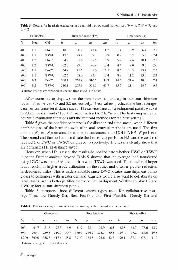
After extensive testing, we set the parameters α1 and α2 in our transshipmentlocation heuristic to 0.8 and 0.2 respectively. These values produced the best average-case performance for distance saved. The service time at transshipment points was setto 20 min, and tw and t s (Sect. 3) were each set to 2 h. We start by first comparing theheuristic evaluation functions and the centroid methods for the base setting.

Table 5 gives the confidence intervals for distance and time saved, when differentcombinations of the heuristic evaluation and centroid methods are used. The firstcolumn (Nc = 4N ) contains the number of customers in the COLL-VRPTW problem.The second and third columns indicate the heuristic type (H1 or H2) and the centroidmethod (i.e. DWC or TWSC) employed, respectively. The results clearly show thatH2 dominates H1 in distance saved.

However, when H2 is used, the results do not indicate whether DWC or TSWCis better. Further analysis beyond Table 5 showed that the average load transferredusing DWC was about 8 % greater than when TSWC was used. The transfer of largerloads results in higher truck utilization on the route, and often a greater reductionin dead-head miles. This is understandable since DWC locates transshipment pointscloser to customers with greater demand. Carriers would also want to collaborate onlarger loads, as this better justifies the work in transshipment. We thus employ H2 andDWC to locate transshipment points.

Table 6 compares three different search types used for collaborative rout-ing. These are Greedy Set, Best Feasible and First Feasible. Greedy Set and

Table 6 Distance savings from collaborative routing with different search methods

Greedy set Best feasible First feasible

Nc le μ ue hw le μ ue hw le μ ue hw

400 64.7 81.6 98.5 16.9 61.9 78.4 94.9 16.5 48.8 62.7 76.6 13.9

800 209.1 259.8 310.5 50.7 196.0 246.2 296.5 50.3 129.4 159.2 189.0 29.8

1,200 300.0 358.8 417.6 58.8 301.0 363.8 426.6 62.8 196.1 237.1 278.1 41.0

Distance savings are reported in km

123


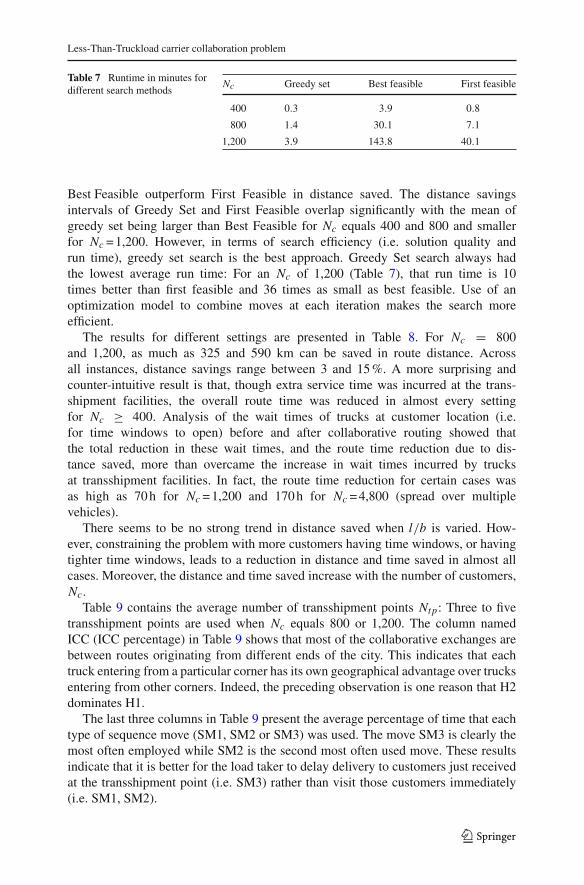
Table 7 Runtime in minutes fordifferent search methods

Nc Greedy set Best feasible First feasible

400 0.3 3.9 0.8

800 1.4 30.1 7.1

1,200 3.9 143.8 40.1

Best Feasible outperform First Feasible in distance saved. The distance savingsintervals of Greedy Set and First Feasible overlap significantly with the mean ofgreedy set being larger than Best Feasible for Nc equals 400 and 800 and smallerfor Nc = 1,200. However, in terms of search efficiency (i.e. solution quality andrun time), greedy set search is the best approach. Greedy Set search always hadthe lowest average run time: For an Nc of 1,200 (Table 7), that run time is 10times better than first feasible and 36 times as small as best feasible. Use of anoptimization model to combine moves at each iteration makes the search moreefficient.

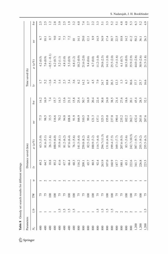
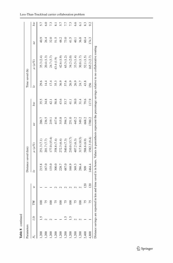
The results for different settings are presented in Table 8. For Nc = 800and 1,200, as much as 325 and 590 km can be saved in route distance. Acrossall instances, distance savings range between 3 and 15 %. A more surprising andcounter-intuitive result is that, though extra service time was incurred at the trans-shipment facilities, the overall route time was reduced in almost every settingfor Nc ≥ 400. Analysis of the wait times of trucks at customer location (i.e.for time windows to open) before and after collaborative routing showed thatthe total reduction in these wait times, and the route time reduction due to dis-tance saved, more than overcame the increase in wait times incurred by trucksat transshipment facilities. In fact, the route time reduction for certain cases wasas high as 70 h for Nc = 1,200 and 170 h for Nc = 4,800 (spread over multiplevehicles).

There seems to be no strong trend in distance saved when l/b is varied. How-ever, constraining the problem with more customers having time windows, or havingtighter time windows, leads to a reduction in distance and time saved in almost allcases. Moreover, the distance and time saved increase with the number of customers,Nc.

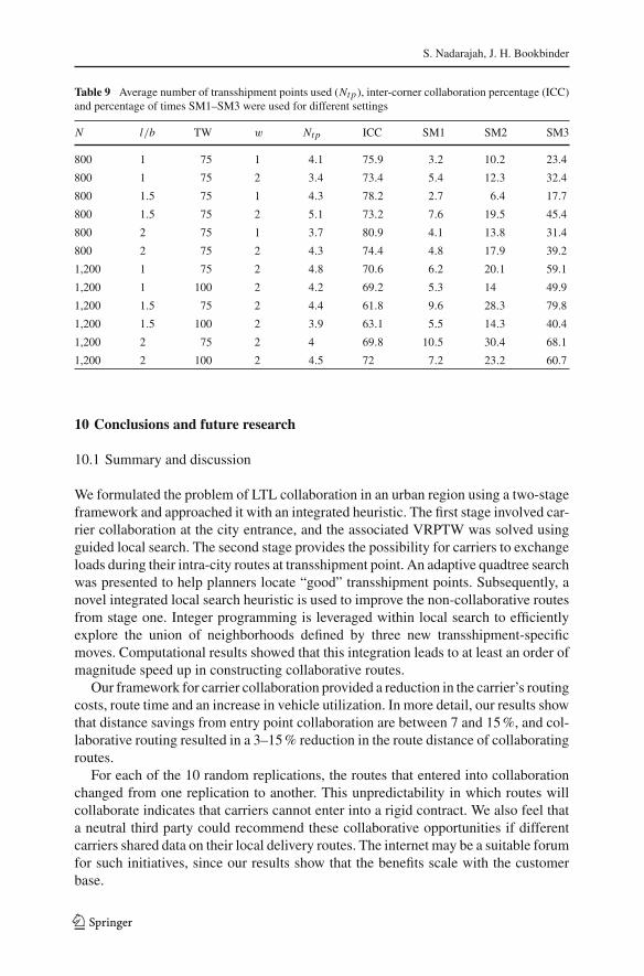
Table 9 contains the average number of transshipment points Ntp: Three to fivetransshipment points are used when Nc equals 800 or 1,200. The column namedICC (ICC percentage) in Table 9 shows that most of the collaborative exchanges arebetween routes originating from different ends of the city. This indicates that eachtruck entering from a particular corner has its own geographical advantage over trucksentering from other corners. Indeed, the preceding observation is one reason that H2dominates H1.

The last three columns in Table 9 present the average percentage of time that eachtype of sequence move (SM1, SM2 or SM3) was used. The move SM3 is clearly themost often employed while SM2 is the second most often used move. These resultsindicate that it is better for the load taker to delay delivery to customers just receivedat the transshipment point (i.e. SM3) rather than visit those customers immediately(i.e. SM1, SM2).

123


Tabl

e8

Gre

edy

sets

earc

hre

sults

for

diff

eren

tset

tings

Para

met

ers

Dis

tanc

esa

ved

(km

)T

ime

save

d(h

)

Nc

l/b

TW

wle

μ(μ

%)

ue

hw

leμ

(μ%

)u

ehw

400

175

149

.263

.3(3

.9)

77.5

14.2

1.7

4.2

(0.5

)6.

72.

5

400

175

264

.781

.6(5

.1)

98.5

16.9

5.2

7.6

(0.9

)10

.12.

5

400

110

01

18.8

26.1

(1.6

)33

.57.

4−1

.6−0

.5(−

0.1)

0.7

1.2

400

110

02

85.2

100.

9(6

.0)

116.

615

.73.

46.

2(0

.7)

9.0

2.8

400

1.5

751

41.6

55.9

(4.1

)70

.214

.31.

45.

2(1

.1)

9 .1

3.9

400

1.5

752

67.7

81.2

(6.2

)94

.813

.62.

34.

8(1

.0)

7.3

2.5

400

1.5

100

166

.487

.6(6

.4)

108.

821

.23.

45.

3(0

.9)

7.2

1.9

400

1.5

100

260

.376

.1(5

.6)

91.9

15.8

3.6

6.8

(1.2

)10

3.2

800

175

111

6.2

141.

5(4

.4)

166.

925

.46.

210

.2(0

.9)

14.1

4.0

800

175

220

9.1

259.

8(8

.2)

310.

550

.714

.221

.6(2

.0)

29.0

7.4

800

110

01

65.7

82.5

(2.6

)99

.416

.96.

79.

4(0

.6)

12.1

2.7

800

110

02

80.5

100.

9(3

.2)

121.

320

.44.

56.

7(0

.8)

8.9

2.2

800

1.5

751

92.4

114.

7(4

.4)

137.

122

.47.

911

.2(1

.0)

14.5

3.3

800

1.5

752

263.

929

4.7(1

1.5)

325.

530

.824

.729

.8(2

.5)

34.9

5.1

800

1.5

100

110

7.0

131.

0(4

.9)

155.

024

.010

.814

.1(1

.0)

17.4

3.3

800

1.5

100

216

0.9

199.

4(7

.5)

237.

838

.520

.325

.5(2

.0)

30.7

5.2

800

275

114

7.7

169.

1(7

.7)

190.

421

.412

.317

.4(1

.6)

22.5

5.1

800

275

218

0.1

207.

6(9

.5)

235.

227

.61.

36.

1(0

.7)

10.8

4.8

800

210

01

65.1

83.7

(3.6

)10

2.2

18.6

6.3

10.3

(0.9

)14

.24.

0

800

210

02

222.

624

2.7(1

0.5)

262.

720

.130

.635

.9(2

.9)

41.2

5.3

1,20

01

751

341.

738

7.1

(9.7

)43

2.4

45.4

37.7

44.0

(2.6

)50

.26.

3

1,20

01

100

122

6.8

255.

3(9

.2)

283.

828

.525

.730

.9(2

.6)

36.1

5.2

1,20

01.

575

122

3.5

255.

5(6

.3)

287.

632

.116

.621

.5(1

.8)

26.3

4.9

123


Tabl

e8

cont

inue

d

Para

met

ers

Dis

tanc

esa

ved

(km

)T

ime

save

d(h

)

Nc

l/b

TW

wle

μ(μ

%)

ue

hw

leμ

(μ%

)u

ehw

1,20

01.

510

01

215.

825

1.3

(7.1

)28

6.7

35.5

29.6

35.3

(2.4

)40

.95.

7

1,20

02

751

167.

020

1.7

(7.7

)23

6.5

34.8

14.4

20.4

(1.3

)26

.46.

0

1,20

02

100

113

5.0

177.

0(1

5.4)

219.

142

.117

.424

.7(3

.7)

32.0

7.3

1,20

01

752

300.

035

8.8

(7.4

)41

7.6

58.8

35.3

43.4

(1.9

)51

.58.

1

1,20

01

100

222

8.7

272.

3(6

.4)

315.

843

.636

.942

.6(1

.9)

48.2

5.7

1,20

01.

575

248

7.0

540.

6(7

.3)

594.

353

.757

.665

.3(1

.2)

73.0

7.7

1,20

01.

510

02

168.

921

0.0

(13.

7)25

1.0

41.1

26.9

34.2

(2.0

)41

.57.

3

1,20

02

752

369.

340

7.2

(6.3

)44

5.2

38.0

26.9

33.5

(1.4

)40

.16.

6

1,20

02

100

228

6.4

317.

8(1

0.5)

349.

231

.424

.730

.8(1

.7)

36.8

6.1

2,40

01

7512

050

958

8.6

(6.9

)66

8.2

79.6

43.8

52.1

(1.5

)60

.48.

3

4,80

01

7512

014

64.4

1582

.3(9

.4)

1700

.211

7.9

156

165.

2(2

.7)

174.

39.

2

Dis

tanc

esa

ving

sar

ere

port

edin

kman

dtim

esa

ved

isin

hour

s.V

alue

sin

pare

nthe

sis

repr

esen

tthe

perc

enta

gesa

ving

sre

lativ

eto

noco

llabo

rativ

ero

utin

g

123


Table 9 Average number of transshipment points used (Ntp), inter-corner collaboration percentage (ICC)and percentage of times SM1–SM3 were used for different settings

N l/b TW w Ntp ICC SM1 SM2 SM3

800 1 75 1 4.1 75.9 3.2 10.2 23.4

800 1 75 2 3.4 73.4 5.4 12.3 32.4

800 1.5 75 1 4.3 78.2 2.7 6.4 17.7

800 1.5 75 2 5.1 73.2 7.6 19.5 45.4

800 2 75 1 3.7 80.9 4.1 13.8 31.4

800 2 75 2 4.3 74.4 4.8 17.9 39.2

1,200 1 75 2 4.8 70.6 6.2 20.1 59.1

1,200 1 100 2 4.2 69.2 5.3 14 49.9

1,200 1.5 75 2 4.4 61.8 9.6 28.3 79.8

1,200 1.5 100 2 3.9 63.1 5.5 14.3 40.4

1,200 2 75 2 4 69.8 10.5 30.4 68.1

1,200 2 100 2 4.5 72 7.2 23.2 60.7

10 Conclusions and future research

10.1 Summary and discussion

We formulated the problem of LTL collaboration in an urban region using a two-stageframework and approached it with an integrated heuristic. The first stage involved car-rier collaboration at the city entrance, and the associated VRPTW was solved usingguided local search. The second stage provides the possibility for carriers to exchangeloads during their intra-city routes at transshipment point. An adaptive quadtree searchwas presented to help planners locate “good” transshipment points. Subsequently, anovel integrated local search heuristic is used to improve the non-collaborative routesfrom stage one. Integer programming is leveraged within local search to efficientlyexplore the union of neighborhoods defined by three new transshipment-specificmoves. Computational results showed that this integration leads to at least an order ofmagnitude speed up in constructing collaborative routes.

Our framework for carrier collaboration provided a reduction in the carrier’s routingcosts, route time and an increase in vehicle utilization. In more detail, our results showthat distance savings from entry point collaboration are between 7 and 15 %, and col-laborative routing resulted in a 3–15 % reduction in the route distance of collaboratingroutes.

For each of the 10 random replications, the routes that entered into collaborationchanged from one replication to another. This unpredictability in which routes willcollaborate indicates that carriers cannot enter into a rigid contract. We also feel thata neutral third party could recommend these collaborative opportunities if differentcarriers shared data on their local delivery routes. The internet may be a suitable forumfor such initiatives, since our results show that the benefits scale with the customerbase.

123


For the values of n that we studied, collaborative routing resulted in route timereductions of between 1 and 4 %. Savings in time will permit the vehicle to return tothe depot early, which may allow the utilization of that vehicle for either a secondlocal delivery or other for-hire purposes. Average truck utilization also increased byat least 4–5 %. This increase makes each vehicle more profitable, and leads to fewerdead-head miles as well.

Those savings in distance and time may furnish the motivation for a city governmentto consider our suggestion on collaboration. Route-time reductions lead to trucksspending less time doing local delivery, which lessens congestion. Cost of congestiondue to trucking in the city of Toronto and neighboring regions was a shocking US$2.3to 3.7 billion in 2002. Therefore, reduction in congestion implied by our model mayhave indirect cost benefits as well. Trucks are the second biggest emitter of green-housegases, and less route time would lead to a reduction in emissions.

However, there are hurdles to implementing a collaborative framework. Firstly,entry-point facilities may need to be owned by the government, since different carriersbenefit from collaboration at different times. Secondly, a mechanism to share savingsfrom collaboration also needs to be formulated. Finally, a highly-trusted, neutral thirdparty is required to facilitate such collaboration. An alternative way to overcome thefirst hurdle is to use a customer’s facility as a transshipment point; some customersmay have larger receiving facilities which can be utilized.

10.2 Future research

One extension of our work is to formulate the COLL-VRPTW as a mathematicalprogramming model. This formulation might then be solved using an optimizationheuristic, or its relaxation could be used to obtain lower bounds. We are currentlypursuing this area. An open research question is, “To what extent will line haul collab-oration help carriers and shippers?” Work on shipper collaboration deals with this issue,but synergies between shipper and carrier collaboration have not yet been explored.A system for sharing collaborative savings between carriers is another question thatneeds further research in our context.

References

Bräysy, O., Gendreau, M.: Vehicle routing with time windows, part 1: route construction and local searchalgorithms. Transp. Sci. 39(1), 104–118 (2005a)

Bräysy, O., Gendreau, M.: Vehicle routing with time windows, part 2: metaheuristics. Transp. Sci. 39(1),119–139 (2005b)

Crainic, T.G., Ricciardi, N., Storchi, G.: Routing vehicles in two-level city logistics systems. In: 50thCanadian Operational Research Society Conference, Université Laval, Québec (2008)

Cruijssen, F., Salomon, M.: Empirical study: Order sharing between transportation companies may resultin cost reductions between 5 to 15 percent. Technical report, Tilburg University, Center for EconomicResearch (2004)

De Backer, B., Furnon, V., Kilby, P., Prosser, P., Shaw, P.: Solving vehicle routing problems using constraintprogramming and metaheuristics. J. Heuristics 6(4), 501–523 (2000)

Ergun, O., Kuyzu, G., Savelsbergh, M.: Shipper collaboration. Comput. Oper. Res. 34(6), 1551–1560 (2007)

123


Finkel, R.A., Bentley, J.L.: Quadtrees: a data stucture for retrieval on composite keys. Acta Inf. 4, 1–9(1974)

Focacci, F., Lodi, A., Milano, M.: Cost-based domain filtering. In: Principles and Practice of ConstraintProgramming-CP99, pp. 189–203. Springer, Berlin (1999)

Hooker, J.N.: Integrated methods for optimization. In: International Series in Operations Research andManagement Science, vol. 100. Springer, New York (2007)

Houghtalen, L., Ergun, Ö., Sokol, J.: Designing mechanisms for the management of carrier alliances. Transp.Sci. 45(4), 465 (2011)

Industry Canada: state of logistics: the canadian report 2008. Technical report, www.ic.gc.ca//logistics(2008)

Jain, A.K., Murty, M.N., Flynn, P.J.: Data clustering: a review. ACM Comput. Surv. 31(3), 264–323 (1999)Jain, V., Grossmann, I.E.: Algorithms for hybrid MILP/CP models for a class of optimization problems.

INFORMS J. Comput. 13(4), 258–276 (2001)Kindervater, G.A.P., Savelsbergh, M.W.P.: Vehicle routing: handling edge exchanges. In: Local Search in

Combinatorial Optimzation, chap. 10, pp. 337–360. Princeton University Press, Princeton (2003)Krajewska, M.A., Kopfer, H.: Collaborating freight forwarding enterprises. OR Spectrum 28(3), 301–317

(2006)Krajewska, M.A., Kopfer, H.: Transportation planning in freight forwarding companies: Tabu search algo-

rithm for the integrated operational transportation planning problem. Eur. J. Oper. Res. 197(2), 741–751(2009)

Liu, R., Jiang, Z., Fung, R.Y.K., Chen, F., Liu, X.: Two-phase heuristic algorithms for full truckloads multi-depot capacitated vehicle routing problem in carrier collaboration. Comput. Oper. Res. 37(5), 950–959(2010)

Lynch, K.: Collaborative logistics networks: breaking traditional performance barriers for shippers andcarriers. White paper, Nistevo, Minneapolis, Minnesota (2001)

Özener, O.Ö., Ergun, Ö., Savelsbergh, M.: Lane-exchange mechanisms for truckload carrier collaboration.Transp. Sci. 45(1), 1–17 (2011)

Rossi, F., Van Beek, P., Walsh, T.: Handbook of knowledge representation. Foundations of Artificial Intel-ligence, chap. 4, pp. 181–212. Elsevier, Amsterdam (2007)

Solomon, M.: Algorithms for the vehicle routing and scheduling problems with time window constraints.Oper. Res. 35(2), 254–265 (1987)

Sutherland, J.L.: Collaborative transportation management: a solution to the current transportation crisis.CVCR white paper 0602, Lehigh University, Pennsylvania (2006)

Taillard, I.D.: Parallel iterative search methods for vehicle routing problems. Networks 23(8), 661–676(1993)

van Hoeve, W.: A hybrid constraint programming and semidefinite programming approach for the stableset problem. In: Principles and Practice of Constraint Programming-CP 2003, pp. 407–421. Springer,Berlin (2003)

Voudouris, C., Tsang, E.: Guided local search. Eur. J. Oper. Re. 113(2), 80–110 (1998)Voudouris, C., Tsang, E.: Handbook of Metaheuristics, vol. 57 of International Series in Operations Research

and Management Science, chap. 7, pp. 185–218. Kluwer, Norwell (2002)Wilson, R.: CSCMP’s annual state of logistics report. Technical report, CSCMP, Lombard, Illinois (2007)Yunes, T.: Success stories in integrated optimization. http://moya.bus.miami.edu/~tallys/integrated.php

(2012)

123

www.ic.gc.ca//logistics

http://moya.bus.miami.edu/~tallys/integrated.php

Download - Less-Than-Truckload carrier collaboration problem: modeling framework and solution approach

Top Related