Investing in Commodities: from Roll Returns toStatistical Arbitrage
Steven Lillywhite
November, 30 2010
Steven Lillywhite () Investing in Commodities November, 30 2010 1 / 49
Overview
1 Investing in Commodities
2 Types of Commodities Investments
3 Backwardation and Contango
4 Convenience Yield
5 Models of Commodity Prices
6 Statistical Arbitrage
7 Natural Gas Trading Disasters
Steven Lillywhite () Investing in Commodities November, 30 2010 2 / 49
Why Invest in Commodities?
Traditional reasons: diversification of portfolio.
Steven Lillywhite () Investing in Commodities November, 30 2010 3 / 49
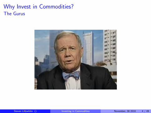
Why Invest in Commodities?The Gurus
Steven Lillywhite () Investing in Commodities November, 30 2010 4 / 49
Why Invest in Commodities?Inflation?
Steven Lillywhite () Investing in Commodities November, 30 2010 5 / 49
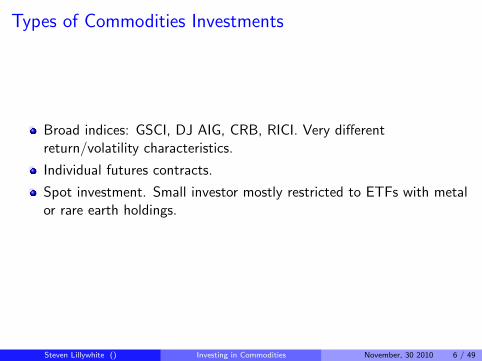
Types of Commodities Investments
Broad indices: GSCI, DJ AIG, CRB, RICI. Very differentreturn/volatility characteristics.
Individual futures contracts.
Spot investment. Small investor mostly restricted to ETFs with metalor rare earth holdings.
Steven Lillywhite () Investing in Commodities November, 30 2010 6 / 49
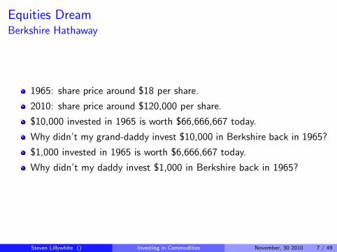
Equities DreamBerkshire Hathaway
1965: share price around $18 per share.
2010: share price around $120,000 per share.
$10,000 invested in 1965 is worth $66,666,667 today.
Why didn’t my grand-daddy invest $10,000 in Berkshire back in 1965?
$1,000 invested in 1965 is worth $6,666,667 today.
Why didn’t my daddy invest $1,000 in Berkshire back in 1965?
Steven Lillywhite () Investing in Commodities November, 30 2010 7 / 49
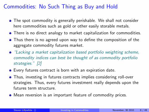
Commodities: No Such Thing as Buy and Hold
The spot commodity is generally perishable. We shall not considerhere commodities such as gold or other easily storable metals.
There is no direct analogy to market capitalization for commodities.
Thus there is no agreed upon way to define the composition of theaggregate commodity futures market.
“Lacking a market capitalization based portfolio weighting scheme,commodity indices can best be thought of as commodity portfoliostrategies.” [2]
Every futures contract is born with an expiration date.
Thus, investing in futures contracts implies considering roll-overstrategies. Thus, every futures investment really depends upon thefutures term structure.
Mean reversion is an important feature of commodity prices.
Steven Lillywhite () Investing in Commodities November, 30 2010 8 / 49
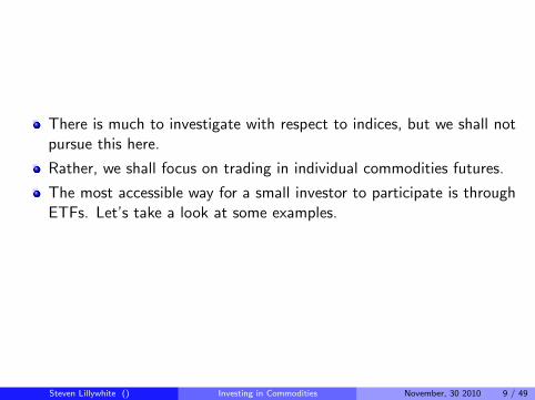
There is much to investigate with respect to indices, but we shall notpursue this here.
Rather, we shall focus on trading in individual commodities futures.
The most accessible way for a small investor to participate is throughETFs. Let’s take a look at some examples.
Steven Lillywhite () Investing in Commodities November, 30 2010 9 / 49
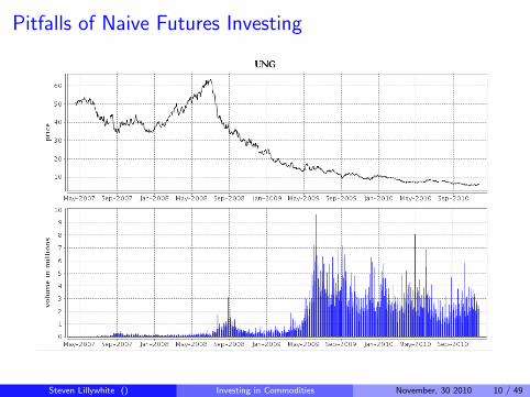
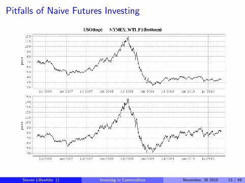
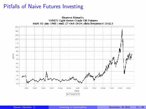
Pitfalls of Naive Futures Investing
Steven Lillywhite () Investing in Commodities November, 30 2010 10 / 49
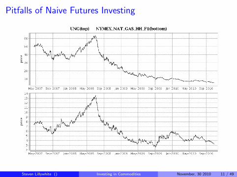
Pitfalls of Naive Futures Investing
Steven Lillywhite () Investing in Commodities November, 30 2010 11 / 49
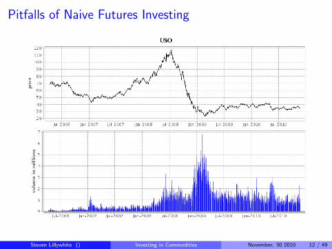
Pitfalls of Naive Futures Investing
Steven Lillywhite () Investing in Commodities November, 30 2010 12 / 49
Pitfalls of Naive Futures Investing
Steven Lillywhite () Investing in Commodities November, 30 2010 13 / 49
Pitfalls of Naive Futures Investing
Steven Lillywhite () Investing in Commodities November, 30 2010 14 / 49
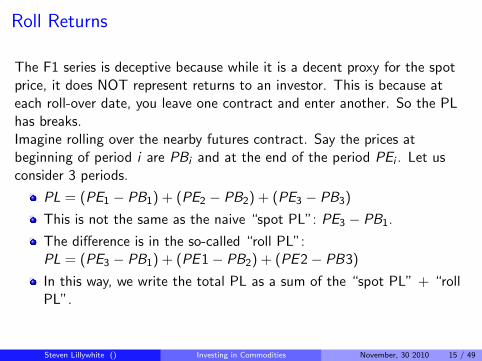
Roll Returns
The F1 series is deceptive because while it is a decent proxy for the spotprice, it does NOT represent returns to an investor. This is because ateach roll-over date, you leave one contract and enter another. So the PLhas breaks.Imagine rolling over the nearby futures contract. Say the prices atbeginning of period i are PBi and at the end of the period PEi . Let usconsider 3 periods.
PL = (PE1 − PB1) + (PE2 − PB2) + (PE3 − PB3)
This is not the same as the naive “spot PL”: PE3 − PB1.
The difference is in the so-called “roll PL”:PL = (PE3 − PB1) + (PE1− PB2) + (PE2− PB3)
In this way, we write the total PL as a sum of the “spot PL” + “rollPL”.
Steven Lillywhite () Investing in Commodities November, 30 2010 15 / 49
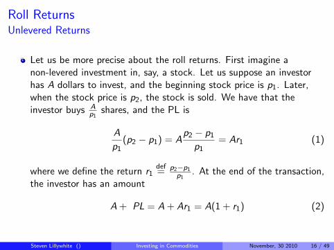
Roll ReturnsUnlevered Returns
Let us be more precise about the roll returns. First imagine anon-levered investment in, say, a stock. Let us suppose an investorhas A dollars to invest, and the beginning stock price is p1. Later,when the stock price is p2, the stock is sold. We have that theinvestor buys A
p1shares, and the PL is
A
p1(p2 − p1) = A
p2 − p1p1
= Ar1 (1)
where we define the return r1def= p2−p1
p1. At the end of the transaction,
the investor has an amount
A + PL = A + Ar1 = A(1 + r1) (2)
Steven Lillywhite () Investing in Commodities November, 30 2010 16 / 49
Roll ReturnsUnlevered Returns
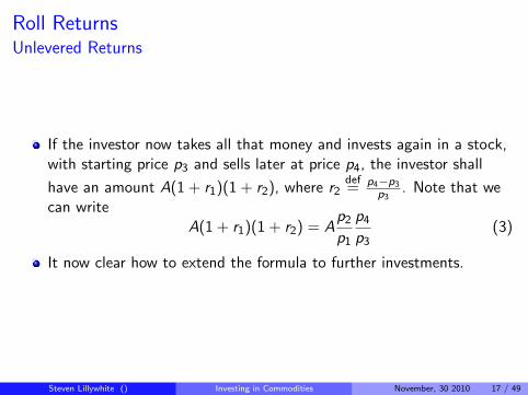
If the investor now takes all that money and invests again in a stock,with starting price p3 and sells later at price p4, the investor shall
have an amount A(1 + r1)(1 + r2), where r2def= p4−p3
p3. Note that we
can writeA(1 + r1)(1 + r2) = A
p2p1
p4p3
(3)
It now clear how to extend the formula to further investments.
Steven Lillywhite () Investing in Commodities November, 30 2010 17 / 49
Roll ReturnsLevered Returns
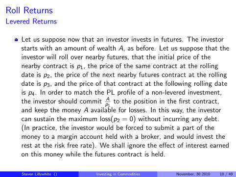
Let us suppose now that an investor invests in futures. The investorstarts with an amount of wealth A, as before. Let us suppose that theinvestor will roll over nearby futures, that the initial price of thenearby contract is p1, the price of the same contract at the rollingdate is p2, the price of the next nearby futures contract at the rollingdate is p3, and the price of that contract at the following rolling dateis p4. In order to match the PL profile of a non-levered investment,the investor should commit A
p1to the position in the first contract,
and keep the money A available for losses. In this way, the investorcan sustain the maximum loss(p2 = 0) without incurring any debt.(In practice, the investor would be forced to submit a part of themoney to a margin account held with a broker, and would invest therest at the risk free rate). We shall ignore the effect of interest earnedon this money while the futures contract is held.
Steven Lillywhite () Investing in Commodities November, 30 2010 18 / 49
Roll ReturnsLevered Returns
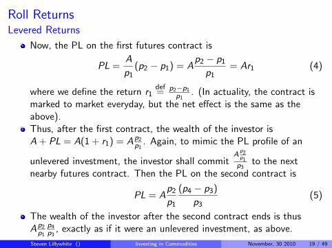
Now, the PL on the first futures contract is
PL =A
p1(p2 − p1) = A
p2 − p1p1
= Ar1 (4)
where we define the return r1def= p2−p1
p1. (In actuality, the contract is
marked to market everyday, but the net effect is the same as theabove).Thus, after the first contract, the wealth of the investor isA + PL = A(1 + r1) = Ap2
p1. Again, to mimic the PL profile of an
unlevered investment, the investor shall commitA
p2p1p3
to the nextnearby futures contract. Then the PL on the second contract is
PL = Ap2p1
(p4 − p3)
p3(5)
The wealth of the investor after the second contract ends is thusAp2
p1p4p3
, exactly as if it were an unlevered investment, as above.
Steven Lillywhite () Investing in Commodities November, 30 2010 19 / 49
Roll ReturnsLevered Returns
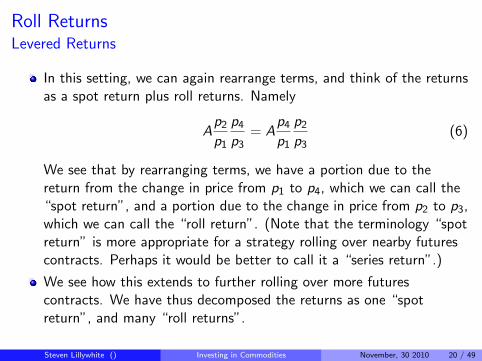
In this setting, we can again rearrange terms, and think of the returnsas a spot return plus roll returns. Namely
Ap2p1
p4p3
= Ap4p1
p2p3
(6)
We see that by rearranging terms, we have a portion due to thereturn from the change in price from p1 to p4, which we can call the“spot return”, and a portion due to the change in price from p2 to p3,which we can call the “roll return”. (Note that the terminology “spotreturn” is more appropriate for a strategy rolling over nearby futurescontracts. Perhaps it would be better to call it a “series return”.)
We see how this extends to further rolling over more futurescontracts. We have thus decomposed the returns as one “spotreturn”, and many “roll returns”.
Steven Lillywhite () Investing in Commodities November, 30 2010 20 / 49
Roll Returns
If the term structure is increasing with time to maturity(contango),then the roll returns are negative.
If the term structure is decreasing with time tomaturity(backwardation), then the roll returns are positive.
Scenarios: imagine spot price constant, term-structure constant; thena rolled futures position consistently makes or loses money dependingon whether there is backwardation or contango.
At first sight it may seem counter-intuitive, but it is possible that thespot price of a commodity could go to infinity, while a rolled futuresposition always loses money! Conversely, spot prices can fall, but arolled futures position can make money nonetheless.
Steven Lillywhite () Investing in Commodities November, 30 2010 21 / 49
Roll ReturnsSummary
Returns on rolled futures positions depend on two main factors. Oneis the change of the spot price. The other is the shape of the termstructure.
For long rolled positions, backwardation helps, contango hurts.
A rolled futures strategy which goes long in a contango market willonly be profitable if the spot price rises even more than the effect ofthe contango.
On the other hand, such a strategy in a backwardated market willalways be profitable if the spot price rises at all, and can even beprofitable if the spot price falls, depending on how much it falls.
Steven Lillywhite () Investing in Commodities November, 30 2010 22 / 49
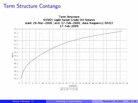
Term Structure Contango
Steven Lillywhite () Investing in Commodities November, 30 2010 23 / 49
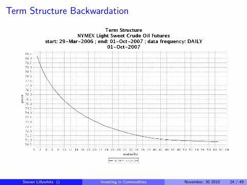
Term Structure Backwardation
Steven Lillywhite () Investing in Commodities November, 30 2010 24 / 49

REMINDER TO THE SPEAKER
Play the term structure movie.
Steven Lillywhite () Investing in Commodities November, 30 2010 25 / 49
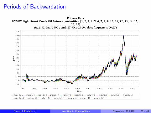
Periods of Backwardation
Steven Lillywhite () Investing in Commodities November, 30 2010 26 / 49
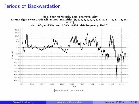
Periods of Backwardation
Steven Lillywhite () Investing in Commodities November, 30 2010 27 / 49
Some Strategies
Oil: go long and wait for wars.
Gas: go long and wait for hurricanes.
Agriculture: go long and wait for droughts.
Momentum strategy: go long backwardated contracts and shortcontangoed contracts with high volatility, [3].
I have not personally checked these strategies .
Steven Lillywhite () Investing in Commodities November, 30 2010 28 / 49
Convenience Yield
Benefits obtained from owning a commodity which are NOT obtainedby holding a futures contract.
Examples include the ability to keep a production process running, orto profit from supply disruptions.
The theory of storage: dates to the 1930s and predicts that the returnfrom purchasing a commodity at time t and selling it for delivery attime T through a futures contract should equal the interest foregoneon the principal plus the storage costs and less the return given by theconvenience yield.
Low inventories and expectations of shortages tend to be associatedwith high convenience yields.
Steven Lillywhite () Investing in Commodities November, 30 2010 29 / 49
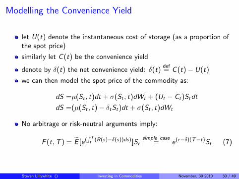
Modelling the Convenience Yield
let U(t) denote the instantaneous cost of storage (as a proportion ofthe spot price)
similarly let C (t) be the convenience yield
denote by δ(t) the net convenience yield: δ(t)def= C (t)− U(t)
we can then model the spot price of the commodity as:
dS =µ(St , t)dt + σ(St , t)dWt + (Ut − Ct)Stdt
dS =(µ(St , t)− δtSt)dt + σ(St , t)dWt
No arbitrage or risk-neutral arguments imply:
F (t,T ) = E [e(∫ Tt (R(s)−δ(s))ds)]St
simple case= e(r−δ)(T−t)St (7)
Steven Lillywhite () Investing in Commodities November, 30 2010 30 / 49
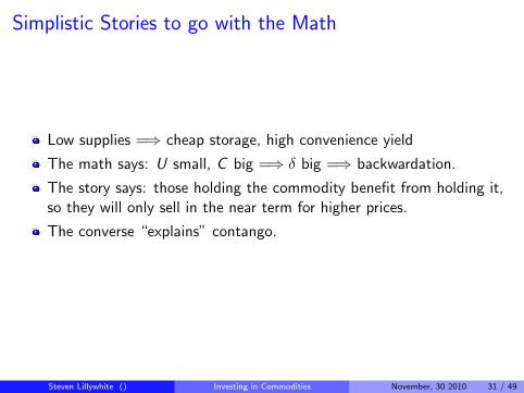
Simplistic Stories to go with the Math
Low supplies =⇒ cheap storage, high convenience yield
The math says: U small, C big =⇒ δ big =⇒ backwardation.
The story says: those holding the commodity benefit from holding it,so they will only sell in the near term for higher prices.
The converse “explains” contango.
Steven Lillywhite () Investing in Commodities November, 30 2010 31 / 49
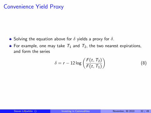
Convenience Yield Proxy
Solving the equation above for δ yields a proxy for δ.
For example, one may take T1 and T2, the two nearest expirations,and form the series
δ = r − 12 log
(F (t,T2)
F (t,T1)
)(8)
Steven Lillywhite () Investing in Commodities November, 30 2010 32 / 49
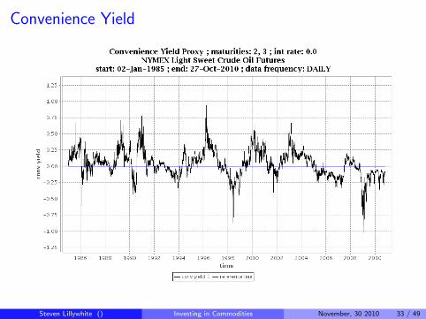
Convenience Yield
Steven Lillywhite () Investing in Commodities November, 30 2010 33 / 49
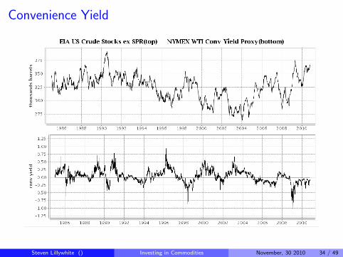
Convenience Yield
Steven Lillywhite () Investing in Commodities November, 30 2010 34 / 49
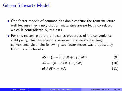
Gibson Schwartz Model
One factor models of commodities don’t capture the term structurewell because they imply that all maturities are perfectly correlated,which is contradicted by the data.
For this reason, plus the time series properties of the convenienceyield proxy, plus the economic reasons for a mean-revertingconvenience yield, the following two-factor model was proposed byGibson and Schwartz.
dS = (µ− δ)Stdt + σ1StdW1 (9)
dδ = κ(θ − δ)dt + σ2dW2 (10)
dW1dW2 = ρdt (11)
Steven Lillywhite () Investing in Commodities November, 30 2010 35 / 49
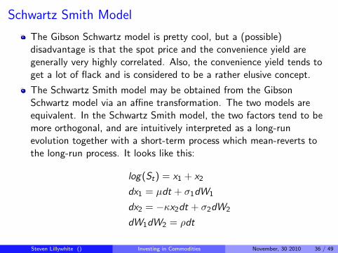
Schwartz Smith Model
The Gibson Schwartz model is pretty cool, but a (possible)disadvantage is that the spot price and the convenience yield aregenerally very highly correlated. Also, the convenience yield tends toget a lot of flack and is considered to be a rather elusive concept.
The Schwartz Smith model may be obtained from the GibsonSchwartz model via an affine transformation. The two models areequivalent. In the Schwartz Smith model, the two factors tend to bemore orthogonal, and are intuitively interpreted as a long-runevolution together with a short-term process which mean-reverts tothe long-run process. It looks like this:
log(St) = x1 + x2
dx1 = µdt + σ1dW1
dx2 = −κx2dt + σ2dW2
dW1dW2 = ρdt
Steven Lillywhite () Investing in Commodities November, 30 2010 36 / 49
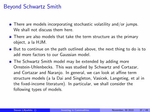
Beyond Schwartz Smith
There are models incorporating stochastic volatility and/or jumps.We shall not discuss them here.
There are also models that take the term structure as the primaryobject, a la HJM.
But to continue on the path outlined above, the next thing to do is toadd more factors to our Gaussian model.
The Schwartz Smith model may be extended by adding moreOrnstein-Uhlenbecks. This was studied by Schwartz and Cortazar,and Cortazar and Naranjo. In general, we can look at affine termstructure models (a la Dai and Singleton, Vasicek, Langetieg, et al inthe fixed-income literature). In particular, we shall consider thefollowing types of models.
Steven Lillywhite () Investing in Commodities November, 30 2010 37 / 49
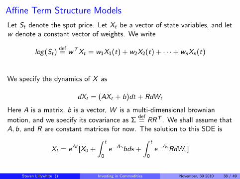
Affine Term Structure Models
Let St denote the spot price. Let Xt be a vector of state variables, and letw denote a constant vector of weights. We write
log(St)def= wTXt = w1X1(t) + w2X2(t) + · · ·+ wnXn(t)
We specify the dynamics of X as
dXt = (AXt + b)dt + RdWt
Here A is a matrix, b is a vector, W is a multi-dimensional brownian
motion, and we specify its covariance as Σdef= RRT . We shall assume that
A, b, and R are constant matrices for now. The solution to this SDE is
Xt = eAt [X0 +
∫ t
0e−Asbds +
∫ t
0e−AsRdWs ]
Steven Lillywhite () Investing in Commodities November, 30 2010 38 / 49
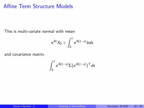
Affine Term Structure Models
This is multi-variate normal with mean
eAtX0 +
∫ t
0eA(t−s)bds
and covariance matrix ∫ t
0eA(t−s)Σ(eA(t−s))Tds
Steven Lillywhite () Investing in Commodities November, 30 2010 39 / 49
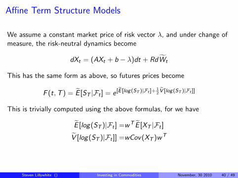
Affine Term Structure Models
We assume a constant market price of risk vector λ, and under change ofmeasure, the risk-neutral dynamics become
dXt = (AXt + b − λ)dt + RdWt
This has the same form as above, so futures prices become
F (t,T ) = E [ST |Ft ] = e [E [log(ST )|Ft ]+12V [log(ST )|Ft ]]
This is trivially computed using the above formulas, for we have
E [log(ST )|Ft ] =wT E [XT |Ft ]
V [log(ST )|Ft ]] =wCov(XT )wT
Steven Lillywhite () Investing in Commodities November, 30 2010 40 / 49
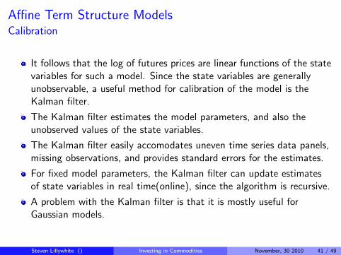
Affine Term Structure ModelsCalibration
It follows that the log of futures prices are linear functions of the statevariables for such a model. Since the state variables are generallyunobservable, a useful method for calibration of the model is theKalman filter.
The Kalman filter estimates the model parameters, and also theunobserved values of the state variables.
The Kalman filter easily accomodates uneven time series data panels,missing observations, and provides standard errors for the estimates.
For fixed model parameters, the Kalman filter can update estimatesof state variables in real time(online), since the algorithm is recursive.
A problem with the Kalman filter is that it is mostly useful forGaussian models.
Steven Lillywhite () Investing in Commodities November, 30 2010 41 / 49
Schwartz Smith 3 and 4
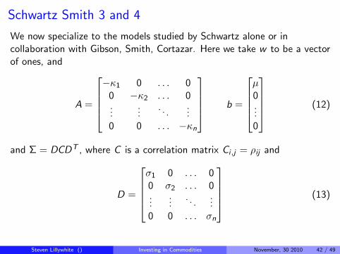
We now specialize to the models studied by Schwartz alone or incollaboration with Gibson, Smith, Cortazar. Here we take w to be a vectorof ones, and
A =
−κ1 0 . . . 0
0 −κ2 . . . 0...
.... . .
...0 0 . . . −κn
b =
µ0...0
(12)
and Σ = DCDT , where C is a correlation matrix Ci ,j = ρij and
D =
σ1 0 . . . 00 σ2 . . . 0...
.... . .
...0 0 . . . σn
(13)
Steven Lillywhite () Investing in Commodities November, 30 2010 42 / 49
Schwartz Smith 3 and 4
The Schwartz Smith model is obtained by exogenously imposingκ1 = 0 in the model above.
I shall call Schwartz Smith 3(4) the model above with 3(4) factorsand κ1 = 0. In these models, the log of the spot is like a BM factor,with an OU mean-reverting to it, with an OU mean-reverting to it,with an OU mean-reverting to it, ...
Fundamental difference with interest rate models is that the spot isnon-stationary, due to the BM factor.
Variations are to change the first BM factor to: i) OU(puremean-reverting model) ii) OU with deterministic drift
Calibrating the pure mean-reversion model for oil or gas after 2000,the mean-reversion rate in the first OU generally goes to zero, sothere is little difference with the Schwartz Smith model.
Steven Lillywhite () Investing in Commodities November, 30 2010 43 / 49

Schwartz Smith 3 and 4Motivation
Why extend the Schwartz Smith model to more factors?
Get better fits to the futures term structure, in particular much betterfit the to term structure of volatilities. (However, this is not to saythat Schwartz Smith 2 does not already do a pretty good job).
PCA. Reminder to speaker: run PCA
Steven Lillywhite () Investing in Commodities November, 30 2010 44 / 49
Statistical Arbitrage
Since our mantra is that every futures investment is a strategy, wemight consider it worth our time and efforts to investigate along thelines of statistical arbitrage.
We have indeed explored several such strategies. Our results lookrather promising.
Steven Lillywhite () Investing in Commodities November, 30 2010 45 / 49
Natural Gas Trading
Amaranth. This was a very large and successful hedge fund based inGreenwich, CT. On September 18th, 2006, the founder of Amaranthinformed investors that the fund had lost an estimated 50% of theirassets month-to-date. By the end of September 2006, the lossesamounted to $6.6 billion, making it the largest hedge fund collapse indollar terms. It was all because of natural gas futures.
In June 2007, the U.S. Senate Permanent Subcommittee onInvestigations(PSI) released a report on “Excessive Speculation in theNatural Gas Market”, [1]. The PSI subpoened trading records fromNYMEX and other sources. As a result, there exists a public record ofAmaranth’s trades. During 2006, Amaranth had large positions inspreads that were of the form: long winter, short summer. Two of thelargest spreads were: long JAN 2007, short NOV 2006, and longMAR 2007, short APR 2007.
Steven Lillywhite () Investing in Commodities November, 30 2010 46 / 49
Natural Gas Trading
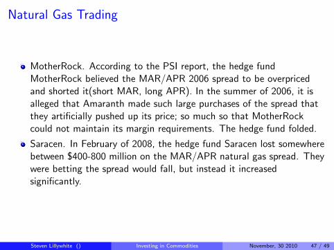
MotherRock. According to the PSI report, the hedge fundMotherRock believed the MAR/APR 2006 spread to be overpricedand shorted it(short MAR, long APR). In the summer of 2006, it isalleged that Amaranth made such large purchases of the spread thatthey artificially pushed up its price; so much so that MotherRockcould not maintain its margin requirements. The hedge fund folded.
Saracen. In February of 2008, the hedge fund Saracen lost somewherebetween $400-800 million on the MAR/APR natural gas spread. Theywere betting the spread would fall, but instead it increasedsignificantly.
Steven Lillywhite () Investing in Commodities November, 30 2010 47 / 49
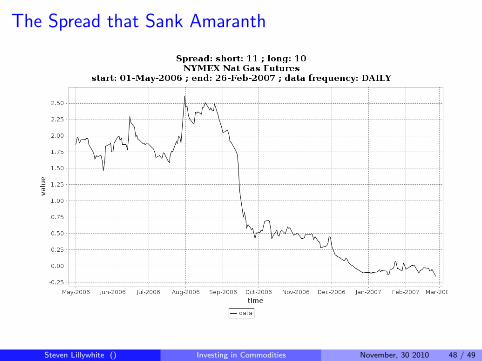
The Spread that Sank Amaranth
Steven Lillywhite () Investing in Commodities November, 30 2010 48 / 49

REMINDER TO THE SPEAKER
Thank the audience.
Steven Lillywhite () Investing in Commodities November, 30 2010 49 / 49
Excessive speculation in the natural gas market.United States Senate Permanent Subcommitte On Investigations,2007.
C.B. Erb and C.R. Harvey.The tactical and strategic value of commodity futures.Financial Analysts Journal, 62(2):69–97, 2006.
J. Miffre and G. Rallis.Momentum strategies in commodity futures markets.Journal of Banking and Finance, 31(6):1863–1886, 2007.
Steven Lillywhite () Investing in Commodities November, 30 2010 49 / 49


