IntroductionWhen linear functions are used to model real-world relationships, the slope and y-intercept of the linear function can be interpreted in context. Recall that data in a scatter plot can be approximated using a linear fit, or linear function that models real-world relationships. A linear fit is the approximation of data using a linear function.
1
4.3.1: Interpreting Slope and y-intercept
Introduction, continued
The slope of a linear function is the change in the
dependent variable divided by the change in the
independent variable, or , sometimes written
as .
2
4.3.1: Interpreting Slope and y-intercept
Introduction, continued
The slope between two points (x1, y1) and (x2, y2) is
, and the slope in the equation y = mx + b is m. The
slope describes how much y changes when x changes
by 1. When analyzing the slope in the context of a real-
world situation, remember to use the units of x and y in
the calculation of the slope.
3
4.3.1: Interpreting Slope and y-intercept
Introduction, continued
For example, if the x-axis of a graph represents hours
and the y-axis represents miles traveled, the slope of a
linear function graphed on these axes would be
, or the miles traveled each hour.
4
4.3.1: Interpreting Slope and y-intercept
Introduction, continuedThe y-intercept of a function is the value of y at which the graph of the function crosses the y-axis, or the value of y when x equals 0. When analyzing the y-intercept in a real-world context, this is the starting value of whatever is represented by the y-axis. For example, if the x-axis represents hours and the y-axis represents miles traveled, the y-intercept would be the miles traveled when the number of hours equals 0. The y-intercept in the equation y = mx + b is b. In some cases, the y-intercept doesn’t make sense in context, such as when the quantity of x equals 0, and the y-intercept is something other than 0 (see Example 2).
5
4.3.1: Interpreting Slope and y-intercept
Key Concepts• The slope of a line with the equation y = mx + b is m.
• The slope of a line is ; the slope between
two points (x1, y1) and (x2, y2) is .
• In context, the slope describes how much the dependent variable changes each time the independent variable changes by 1 unit.
6
4.3.1: Interpreting Slope and y-intercept
Key Concepts, continued• The y-intercept of a line with the equation y = mx + b
is b.
• The y-intercept is the value of y at which a graph crosses the y-axis.
• In context, the y-intercept is the initial value of the quantity represented by the y-axis, or the quantity of y when the quantity represented by the x-axis equals 0.
7
4.3.1: Interpreting Slope and y-intercept
Common Errors/Misconceptions• incorrectly calculating the slope
• confusing the y- and x-intercepts, both in context and when calculating using a graph or equation
8
4.3.1: Interpreting Slope and y-intercept
Guided Practice
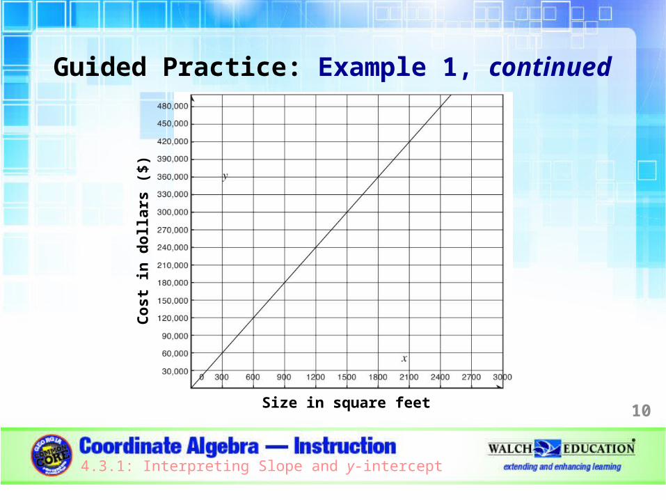
Example 1The graph on the next slide contains a linear model that approximates the relationship between the size of a home and how much it costs. The x-axis represents size in square feet, and the y-axis represents cost in dollars. Describe what the slope and the y-intercept of the linear model mean in terms of housing prices.
9
4.3.1: Interpreting Slope and y-intercept
Guided Practice: Example 1, continued
10
4.3.1: Interpreting Slope and y-intercept
Co
st in
do
llars
($)
Size in square feet
Guided Practice: Example 1, continued
1. Find the equation of the linear fit.The general equation of a line in slope-intercept form is y = mx + b, where m is the slope and b is the y-intercept.
Find two points on the line using the graph.
The graph contains the points (300, 60,000) and (600, 120,000).
11
4.3.1: Interpreting Slope and y-intercept
Guided Practice: Example 1, continued
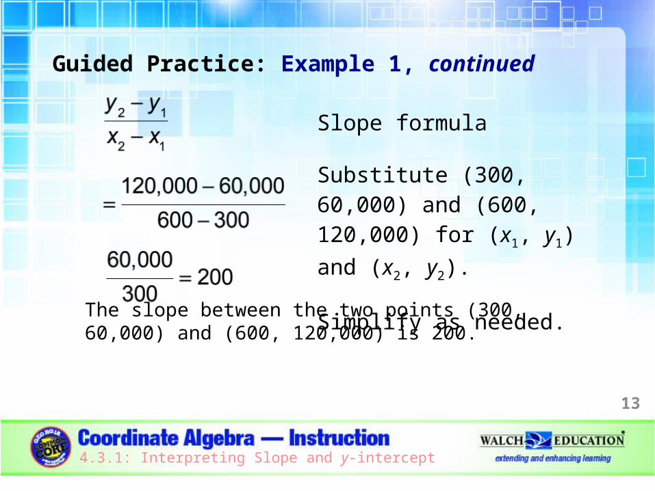
The formula to find the slope between two points
(x1, y1) and (x2, y2) is .
Substitute (300, 60,000) and (600, 120,000) into the
formula to find the slope.
12
4.3.1: Interpreting Slope and y-intercept
Guided Practice: Example 1, continued
The slope between the two points (300, 60,000) and (600, 120,000) is 200.
13
4.3.1: Interpreting Slope and y-intercept
Slope formula
Substitute (300, 60,000) and (600, 120,000) for (x1, y1) and (x2, y2).
Simplify as needed.
Guided Practice: Example 1, continuedFind the y-intercept. Use the equation for slope-intercept form, y = mx + b, where b is the y-intercept.
Replace x and y with values from a single point on the line. Let’s use (300, 60,000).
Replace m with the slope, 200. Solve for b.
14
4.3.1: Interpreting Slope and y-intercept

Guided Practice: Example 1, continued
The y-intercept of the linear model is 0.
The equation of the line is y = 200x.
15
4.3.1: Interpreting Slope and y-intercept
y = mx + b Equation for slope-intercept form
60,000 = 200(300) + b Substitute values for x, y, and m.
60,000 = 60,000 + b Multiply.
0 = b Subtract 60,000 from both sides.
Guided Practice: Example 1, continued
2. Determine the units of the slope.Divide the units on the y-axis by the units on the
x-axis: .
The units of the slope are dollars per square foot.
16
4.3.1: Interpreting Slope and y-intercept
Guided Practice: Example 1, continued
3. Describe what the slope means in context.The slope is the change in cost of the home for each square foot of the home. The slope describes how price is affected by the size of the home purchased. A positive slope means the quantity represented by the y-axis increases when the quantity represented by the x-axis also increases.
The cost of the home increases by $200 for each square foot.
17
4.3.1: Interpreting Slope and y-intercept
Guided Practice: Example 1, continued
4. Determine the units of the y-intercept.The units of the y-intercept are the units of the y-axis: dollars.
18
4.3.1: Interpreting Slope and y-intercept
Guided Practice: Example 1, continued
5. Describe what the y-intercept means in context.The y-intercept is the value of the equation when x = 0, or when the size of the home is 0 square feet. For a home with no area, or for no home, the cost is $0.
19
4.3.1: Interpreting Slope and y-intercept
✔

Guided Practice: Example 1, continued
20
4.3.1: Interpreting Slope and y-intercept

Guided Practice
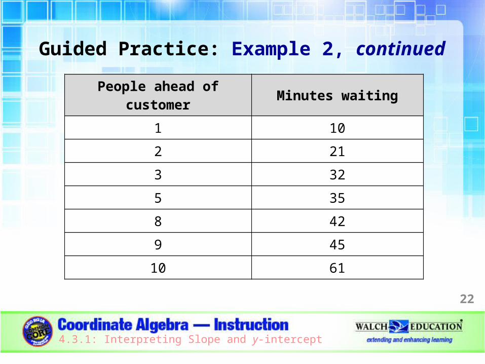
Example 2A teller at a bank records the amount of time a customer waits in line and the number of people in line ahead of that customer when he or she entered the line. Describe the relationship between waiting time and the people ahead of a customer when the customer enters a line. Use the table on the following slide.
21
4.3.1: Interpreting Slope and y-intercept
Guided Practice: Example 2, continued
22
4.3.1: Interpreting Slope and y-intercept
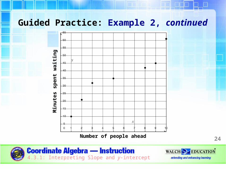
People ahead of customer Minutes waiting
1 10
2 21
3 32
5 35
8 42
9 45
10 61
Guided Practice: Example 2, continued
1. Create a scatter plot of the data. Let the x-axis represent the number of people ahead of the customer and the y-axis represent the minutes spent waiting.
23
4.3.1: Interpreting Slope and y-intercept
Guided Practice: Example 2, continued
24
4.3.1: Interpreting Slope and y-intercept
Min
ute
s sp
ent
wai
tin
g
Number of people ahead
Guided Practice: Example 2, continued2. Find the equation of a linear model to
represent the data.Use two points to estimate a linear model. A line through the two points should have approximately the same number of data values both above and below the line. A line through the first and last data points, (1, 10) and (10, 61), appears to be a good approximation of the data. Find the slope.
25
4.3.1: Interpreting Slope and y-intercept
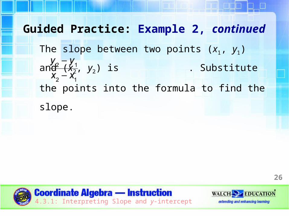
Guided Practice: Example 2, continued
The slope between two points (x1, y1) and (x2, y2) is
. Substitute the points into the formula to find
the slope.
26
4.3.1: Interpreting Slope and y-intercept
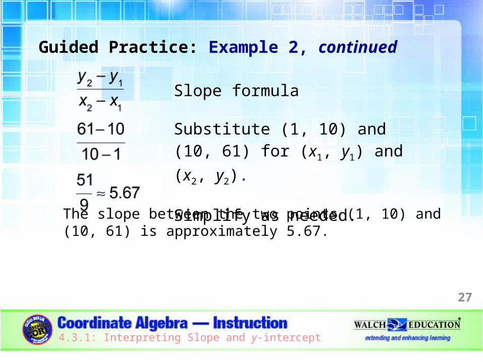
Guided Practice: Example 2, continued
The slope between the two points (1, 10) and (10, 61) is approximately 5.67.
27
4.3.1: Interpreting Slope and y-intercept
Slope formula
Substitute (1, 10) and (10, 61) for (x1, y1) and (x2, y2).
Simplify as needed.
Guided Practice: Example 2, continuedFind the y-intercept. Use the equation for slope-intercept form, y = mx + b, where b is the y-intercept.
Replace x and y with values from a single point on the line. Let’s use (1, 10).
Replace m with the slope, 5.67. Solve for b.
28
4.3.1: Interpreting Slope and y-intercept
Guided Practice: Example 2, continued
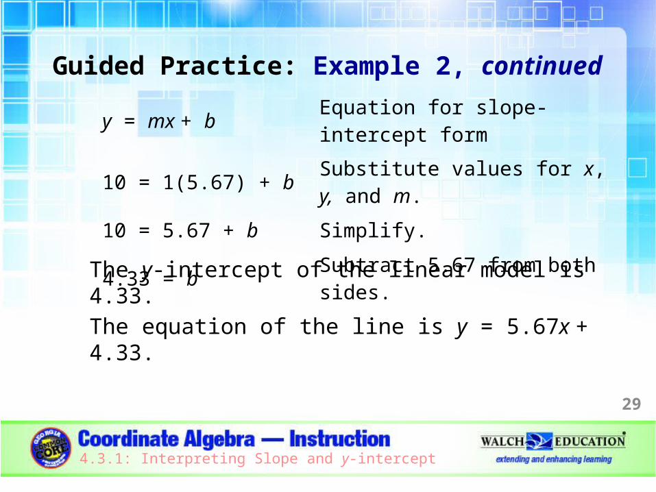
The y-intercept of the linear model is 4.33.
The equation of the line is y = 5.67x + 4.33.
29
4.3.1: Interpreting Slope and y-intercept
y = mx + b Equation for slope-intercept form
10 = 1(5.67) + b Substitute values for x, y, and m.
10 = 5.67 + b Simplify.
4.33 = b Subtract 5.67 from both sides.
Guided Practice: Example 2, continued
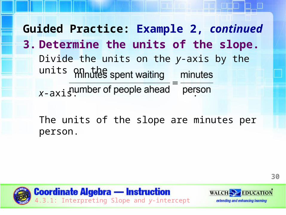
3. Determine the units of the slope.Divide the units on the y-axis by the units on the
x-axis: .
The units of the slope are minutes per person.
30
4.3.1: Interpreting Slope and y-intercept
Guided Practice: Example 2, continued
4. Describe what the slope means in context.The slope describes how the waiting time increases for each person in line ahead of the customer. A customer waits approximately 5.67 minutes for each person who is in line ahead of the customer.
31
4.3.1: Interpreting Slope and y-intercept
Guided Practice: Example 2, continued
5. Determine the units of the y-intercept.The units of the y-intercept are the units of the y-axis: minutes.
32
4.3.1: Interpreting Slope and y-intercept
Guided Practice: Example 2, continued
6. Describe what the y-intercept means in context.The y-intercept is the value of the equation when x = 0, or when the number of people ahead of the customer is 0. The y-intercept is 4.33. In this context, the y-intercept isn’t relevant, because if no one was in line ahead of a customer, the wait time would be 0 minutes. Creating a linear model that matched the data resulted in a y-intercept that wasn’t 0, but this value isn’t related to the context of the situation.
33
4.3.1: Interpreting Slope and y-intercept
✔

Guided Practice: Example 2, continued
34
4.3.1: Interpreting Slope and y-intercept


