Introduction Some basic ideas from Probability Coupon Collection Quick Sort Min Cut
Introduction to Randomized Algorithms
Arijit Bishnu([email protected])
Advanced Computing and Microelectronics UnitIndian Statistical Institute
Kolkata 700108, India.

Introduction Some basic ideas from Probability Coupon Collection Quick Sort Min Cut
Organization
1 Introduction
2 Some basic ideas from Probability
3 Coupon Collection
4 Quick Sort
5 Min Cut
Introduction Some basic ideas from Probability Coupon Collection Quick Sort Min Cut
Introduction
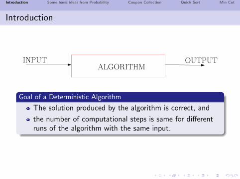
INPUT OUTPUTALGORITHM
Goal of a Deterministic Algorithm
The solution produced by the algorithm is correct, and
the number of computational steps is same for differentruns of the algorithm with the same input.
Introduction Some basic ideas from Probability Coupon Collection Quick Sort Min Cut
Randomized Algorithm
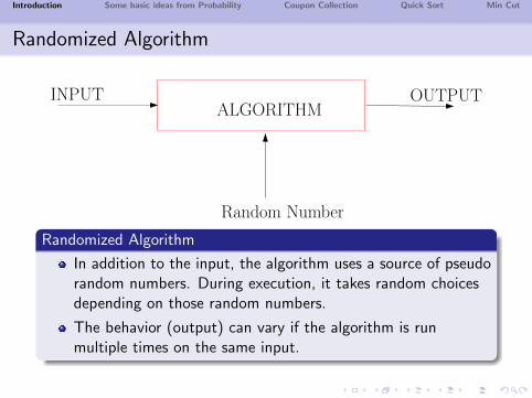
INPUT OUTPUTALGORITHM
Random Number
Randomized Algorithm
In addition to the input, the algorithm uses a source of pseudorandom numbers. During execution, it takes random choicesdepending on those random numbers.
The behavior (output) can vary if the algorithm is runmultiple times on the same input.
Introduction Some basic ideas from Probability Coupon Collection Quick Sort Min Cut
Advantage of Randomized Algorithm
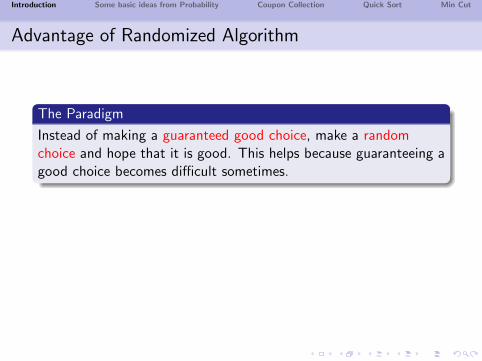
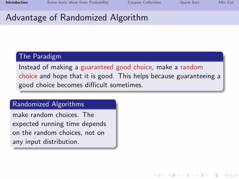
The Paradigm
Instead of making a guaranteed good choice, make a randomchoice and hope that it is good. This helps because guaranteeing agood choice becomes difficult sometimes.
Randomized Algorithms
make random choices. Theexpected running time dependson the random choices, not onany input distribution.
Average Case Analysis
analyzes the expected runningtime of deterministic algorithmsassuming a suitable randomdistribution on the input.
Introduction Some basic ideas from Probability Coupon Collection Quick Sort Min Cut
Advantage of Randomized Algorithm
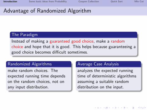
The Paradigm
Instead of making a guaranteed good choice, make a randomchoice and hope that it is good. This helps because guaranteeing agood choice becomes difficult sometimes.
Randomized Algorithms
make random choices. Theexpected running time dependson the random choices, not onany input distribution.
Average Case Analysis
analyzes the expected runningtime of deterministic algorithmsassuming a suitable randomdistribution on the input.
Introduction Some basic ideas from Probability Coupon Collection Quick Sort Min Cut
Pros and Cons of Randomized Algorithms
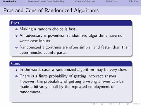
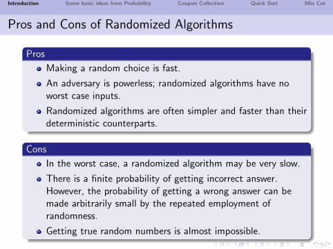
Pros
Making a random choice is fast.
An adversary is powerless; randomized algorithms have noworst case inputs.
Randomized algorithms are often simpler and faster than theirdeterministic counterparts.
Cons
In the worst case, a randomized algorithm may be very slow.
There is a finite probability of getting incorrect answer.However, the probability of getting a wrong answer can bemade arbitrarily small by the repeated employment ofrandomness.
Getting true random numbers is almost impossible.
Introduction Some basic ideas from Probability Coupon Collection Quick Sort Min Cut
Pros and Cons of Randomized Algorithms
Pros
Making a random choice is fast.
An adversary is powerless; randomized algorithms have noworst case inputs.
Randomized algorithms are often simpler and faster than theirdeterministic counterparts.
Cons
In the worst case, a randomized algorithm may be very slow.
There is a finite probability of getting incorrect answer.However, the probability of getting a wrong answer can bemade arbitrarily small by the repeated employment ofrandomness.
Getting true random numbers is almost impossible.
Introduction Some basic ideas from Probability Coupon Collection Quick Sort Min Cut
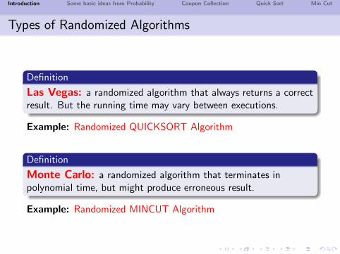
Types of Randomized Algorithms
Definition
Las Vegas: a randomized algorithm that always returns a correctresult. But the running time may vary between executions.
Example: Randomized QUICKSORT Algorithm
Definition
Monte Carlo: a randomized algorithm that terminates inpolynomial time, but might produce erroneous result.
Example: Randomized MINCUT Algorithm
Introduction Some basic ideas from Probability Coupon Collection Quick Sort Min Cut
Some basic ideasfrom Probability

Introduction Some basic ideas from Probability Coupon Collection Quick Sort Min Cut
Expectation
Random variable
A function defined on a sample space is called a random variable.Given a random variable X , Pr [X = j ] means X ’s probability oftaking the value j .
Expectation – “the average value”
The expectation of a random variable X is defined as:E [X ] =
∑∞j=0 j · Pr [X = j ]
Introduction Some basic ideas from Probability Coupon Collection Quick Sort Min Cut
Waiting for the first success
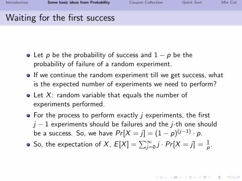
Let p be the probability of success and 1− p be theprobability of failure of a random experiment.
If we continue the random experiment till we get success, whatis the expected number of experiments we need to perform?
Let X : random variable that equals the number ofexperiments performed.
For the process to perform exactly j experiments, the firstj − 1 experiments should be failures and the j-th one shouldbe a success. So, we have Pr [X = j ] = (1− p)(j−1) · p.
So, the expectation of X , E [X ] =∑∞
j=0 j · Pr [X = j ] = 1p .
Introduction Some basic ideas from Probability Coupon Collection Quick Sort Min Cut
Waiting for the first success
Let p be the probability of success and 1− p be theprobability of failure of a random experiment.
If we continue the random experiment till we get success, whatis the expected number of experiments we need to perform?
Let X : random variable that equals the number ofexperiments performed.
For the process to perform exactly j experiments, the firstj − 1 experiments should be failures and the j-th one shouldbe a success. So, we have Pr [X = j ] = (1− p)(j−1) · p.
So, the expectation of X , E [X ] =∑∞
j=0 j · Pr [X = j ] = 1p .
Introduction Some basic ideas from Probability Coupon Collection Quick Sort Min Cut
Conditional Probability and Independent Event
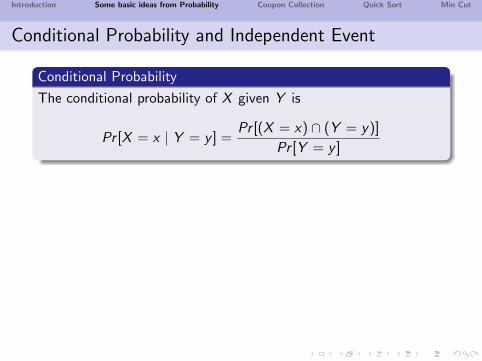
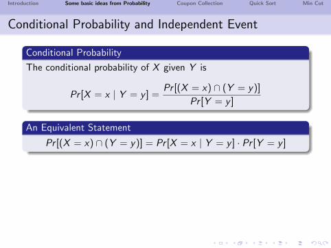
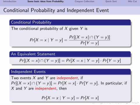
Conditional Probability
The conditional probability of X given Y is
Pr [X = x | Y = y ] =Pr [(X = x) ∩ (Y = y)]
Pr [Y = y ]
An Equivalent Statement
Pr [(X = x) ∩ (Y = y)] = Pr [X = x | Y = y ] · Pr [Y = y ]
Independent Events
Two events X and Y are independent, ifPr [(X = x) ∩ (Y = y)] = Pr [X = x ] · Pr [Y = y ]. In particular, ifX and Y are independent, then
Pr [X = x | Y = y ] = Pr [X = x ]
Introduction Some basic ideas from Probability Coupon Collection Quick Sort Min Cut
Conditional Probability and Independent Event
Conditional Probability
The conditional probability of X given Y is
Pr [X = x | Y = y ] =Pr [(X = x) ∩ (Y = y)]
Pr [Y = y ]
An Equivalent Statement
Pr [(X = x) ∩ (Y = y)] = Pr [X = x | Y = y ] · Pr [Y = y ]
Independent Events
Two events X and Y are independent, ifPr [(X = x) ∩ (Y = y)] = Pr [X = x ] · Pr [Y = y ]. In particular, ifX and Y are independent, then
Pr [X = x | Y = y ] = Pr [X = x ]
Introduction Some basic ideas from Probability Coupon Collection Quick Sort Min Cut
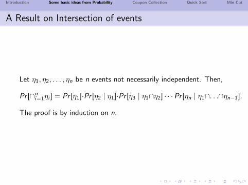
A Result on Intersection of events
Let η1, η2, . . . , ηn be n events not necessarily independent. Then,
Pr [∩ni=1ηi ] = Pr [η1]·Pr [η2 | η1]·Pr [η3 | η1∩η2] · · ·Pr [ηn | η1∩. . .∩ηn−1].
The proof is by induction on n.

Introduction Some basic ideas from Probability Coupon Collection Quick Sort Min Cut
Coupon Collection

Introduction Some basic ideas from Probability Coupon Collection Quick Sort Min Cut
Coupon Collection
The Problem
A company selling jeans gives a coupon with each jeans. There aren different coupons. Collecting n different coupons would give youa free jeans. How many jeans do you expect to buy before you geta free jeans?
The coupon collection process is in phase j when you havealready collected j different coupons and are buying to get anew type.
A new type of coupon ends phase j and you enter phase j + 1.
Introduction Some basic ideas from Probability Coupon Collection Quick Sort Min Cut
Coupon Collection
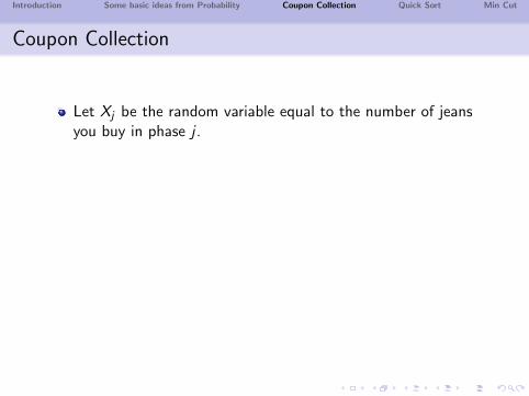
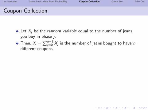
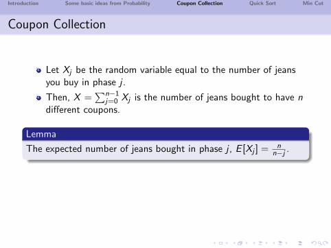
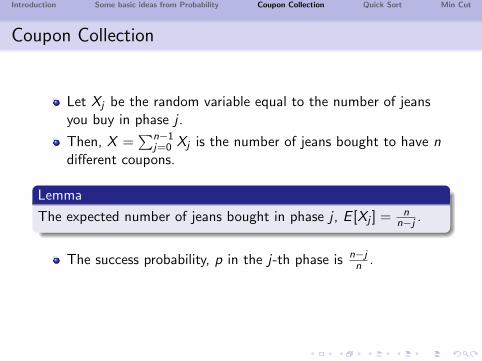
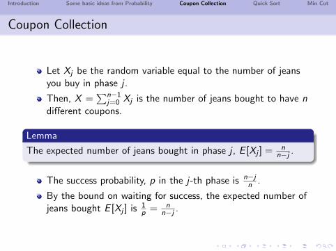
Let Xj be the random variable equal to the number of jeansyou buy in phase j .
Then, X =∑n−1
j=0 Xj is the number of jeans bought to have ndifferent coupons.
Lemma
The expected number of jeans bought in phase j , E [Xj ] = nn−j .
The success probability, p in the j-th phase is n−jn .
By the bound on waiting for success, the expected number ofjeans bought E [Xj ] is 1
p = nn−j .
Introduction Some basic ideas from Probability Coupon Collection Quick Sort Min Cut
Coupon Collection
Let Xj be the random variable equal to the number of jeansyou buy in phase j .
Then, X =∑n−1
j=0 Xj is the number of jeans bought to have ndifferent coupons.
Lemma
The expected number of jeans bought in phase j , E [Xj ] = nn−j .
The success probability, p in the j-th phase is n−jn .
By the bound on waiting for success, the expected number ofjeans bought E [Xj ] is 1
p = nn−j .
Introduction Some basic ideas from Probability Coupon Collection Quick Sort Min Cut
The expectation
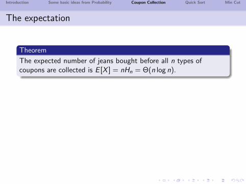
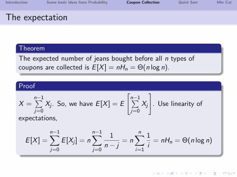
Theorem
The expected number of jeans bought before all n types ofcoupons are collected is E [X ] = nHn = Θ(n log n).
Proof
X =n−1∑j=0
Xj . So, we have E [X ] = E
[n−1∑j=0
Xj
]. Use linearity of
expectations,
E [X ] =n−1∑j=0
E [Xj ] = nn−1∑j=0
1
n − j= n
n∑i=1
1
i= nHn = Θ(n log n)
Introduction Some basic ideas from Probability Coupon Collection Quick Sort Min Cut
The expectation
Theorem
The expected number of jeans bought before all n types ofcoupons are collected is E [X ] = nHn = Θ(n log n).
Proof
X =n−1∑j=0
Xj . So, we have E [X ] = E
[n−1∑j=0
Xj
]. Use linearity of
expectations,
E [X ] =n−1∑j=0
E [Xj ] = nn−1∑j=0
1
n − j= n
n∑i=1
1
i= nHn = Θ(n log n)

Introduction Some basic ideas from Probability Coupon Collection Quick Sort Min Cut
Randomized Quick Sort
Introduction Some basic ideas from Probability Coupon Collection Quick Sort Min Cut
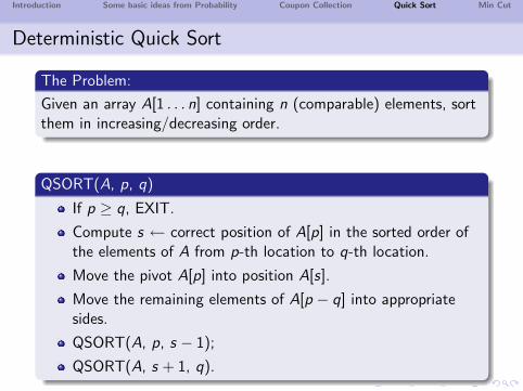
Deterministic Quick Sort
The Problem:
Given an array A[1 . . . n] containing n (comparable) elements, sortthem in increasing/decreasing order.
QSORT(A, p, q)
If p ≥ q, EXIT.
Compute s ← correct position of A[p] in the sorted order ofthe elements of A from p-th location to q-th location.
Move the pivot A[p] into position A[s].
Move the remaining elements of A[p − q] into appropriatesides.
QSORT(A, p, s − 1);
QSORT(A, s + 1, q).
Introduction Some basic ideas from Probability Coupon Collection Quick Sort Min Cut
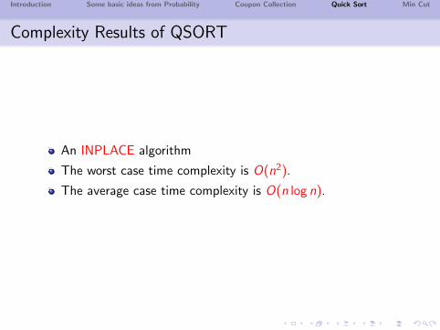
Complexity Results of QSORT
An INPLACE algorithm
The worst case time complexity is O(n2).
The average case time complexity is O(n log n).
Introduction Some basic ideas from Probability Coupon Collection Quick Sort Min Cut
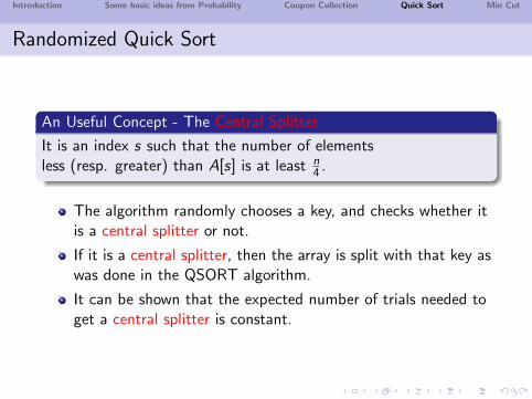
Randomized Quick Sort
An Useful Concept - The Central Splitter
It is an index s such that the number of elementsless (resp. greater) than A[s] is at least n
4 .
The algorithm randomly chooses a key, and checks whether itis a central splitter or not.
If it is a central splitter, then the array is split with that key aswas done in the QSORT algorithm.
It can be shown that the expected number of trials needed toget a central splitter is constant.
Introduction Some basic ideas from Probability Coupon Collection Quick Sort Min Cut
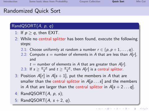
Randomized Quick Sort
RandQSORT(A, p, q)
1: If p ≥ q, then EXIT.
2: While no central splitter has been found, execute the followingsteps:
2.1: Choose uniformly at random a number r ∈ {p, p + 1, . . . , q}.2.2: Compute s = number of elements in A that are less than A[r ],
andt = number of elements in A that are greater than A[r ].
2.3: If s ≥ q−p4 and t ≥ q−p
4 , then A[r ] is a central splitter.
3: Position A[r ] in A[s + 1], put the members in A that aresmaller than the central splitter in A[p . . . s] and the membersin A that are larger than the central splitter in A[s + 2 . . . q].
4: RandQSORT(A, p, s);
5: RandQSORT(A, s + 2, q).
Introduction Some basic ideas from Probability Coupon Collection Quick Sort Min Cut
Analysis of RandQSORT
Fact: One execution of Step 2 needs O(q − p) time.
Question: How many times Step 2 is executed for finding acentral splitter ?
Result:
The probability that the randomly chosen element is a centralsplitter is 1
2 .
Introduction Some basic ideas from Probability Coupon Collection Quick Sort Min Cut
Recall “Waiting for success”
If p be the probability of success of a random experiment, and wecontinue the random experiment till we get success, the expectednumber of experiments we need to perform is 1
p .
Implication in Our Case
The expected number of times Step 2 needs to be repeated toget a central splitter (success) is 2 as the correspondingsuccess probability is 1
2 .
Thus, the expected time complexity of Step 2 is O(n)
Introduction Some basic ideas from Probability Coupon Collection Quick Sort Min Cut
Analysis of RandQSORT
Time Complexity
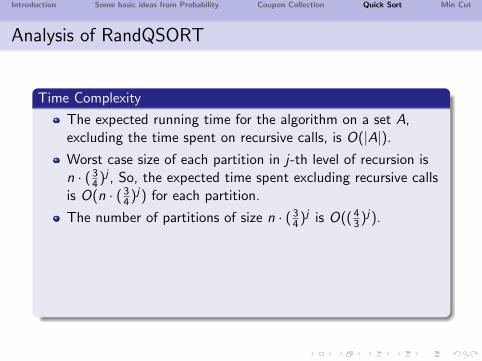
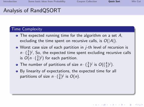
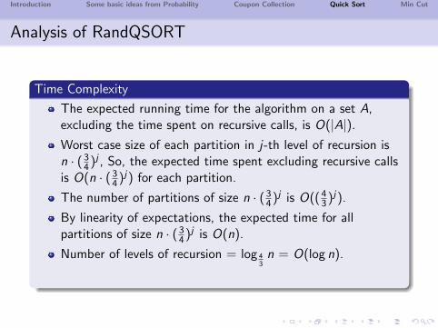
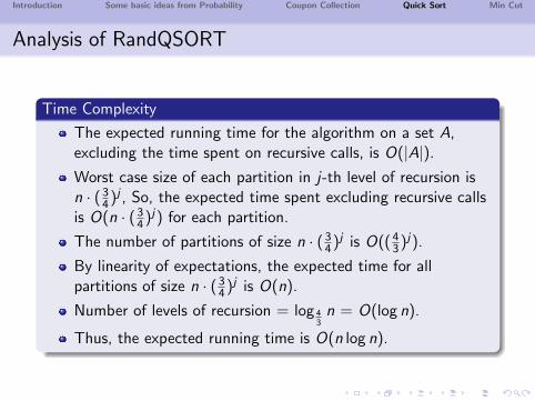
The expected running time for the algorithm on a set A,excluding the time spent on recursive calls, is O(|A|).
Worst case size of each partition in j-th level of recursion isn · (3
4)j , So, the expected time spent excluding recursive callsis O(n · (3
4)j) for each partition.
The number of partitions of size n · (34)j is O((4
3)j).
By linearity of expectations, the expected time for allpartitions of size n · (3
4)j is O(n).
Number of levels of recursion = log 43n = O(log n).
Thus, the expected running time is O(n log n).
Introduction Some basic ideas from Probability Coupon Collection Quick Sort Min Cut
Analysis of RandQSORT
Time Complexity
The expected running time for the algorithm on a set A,excluding the time spent on recursive calls, is O(|A|).
Worst case size of each partition in j-th level of recursion isn · (3
4)j , So, the expected time spent excluding recursive callsis O(n · (3
4)j) for each partition.
The number of partitions of size n · (34)j is O((4
3)j).
By linearity of expectations, the expected time for allpartitions of size n · (3
4)j is O(n).
Number of levels of recursion = log 43n = O(log n).
Thus, the expected running time is O(n log n).
Introduction Some basic ideas from Probability Coupon Collection Quick Sort Min Cut
Finding the k-th largest
Median Finding
Similar ideas of getting a central splitter and waiting for successbound applies for finding the median in O(n) time.

Introduction Some basic ideas from Probability Coupon Collection Quick Sort Min Cut
Global Mincut Problemfor an Undirected Graph
Introduction Some basic ideas from Probability Coupon Collection Quick Sort Min Cut
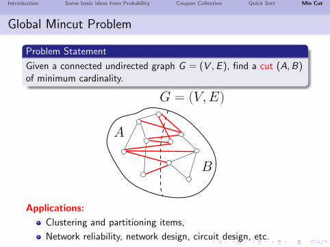
Global Mincut Problem
Problem Statement
Given a connected undirected graph G = (V ,E ), find a cut (A,B)of minimum cardinality.
A
B
G = (V, E)
Applications:
Clustering and partitioning items,
Network reliability, network design, circuit design, etc.
Introduction Some basic ideas from Probability Coupon Collection Quick Sort Min Cut
A Simple Randomized Algorithm
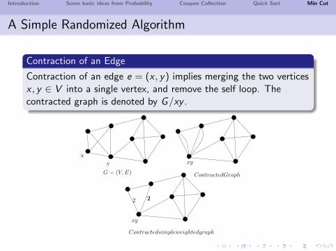
Contraction of an Edge
Contraction of an edge e = (x , y) implies merging the two verticesx , y ∈ V into a single vertex, and remove the self loop. Thecontracted graph is denoted by G/xy .
x
y xy
xy
222
G = (V, E) ContractedGraph
Contractedsimpleweightedgraph
Introduction Some basic ideas from Probability Coupon Collection Quick Sort Min Cut
Results on Contraction of Edges
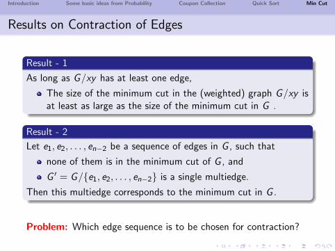
Result - 1
As long as G/xy has at least one edge,
The size of the minimum cut in the (weighted) graph G/xy isat least as large as the size of the minimum cut in G .
Result - 2
Let e1, e2, . . . , en−2 be a sequence of edges in G , such that
none of them is in the minimum cut of G , and
G ′ = G/{e1, e2, . . . , en−2} is a single multiedge.
Then this multiedge corresponds to the minimum cut in G .
Problem: Which edge sequence is to be chosen for contraction?
Introduction Some basic ideas from Probability Coupon Collection Quick Sort Min Cut
Analysis
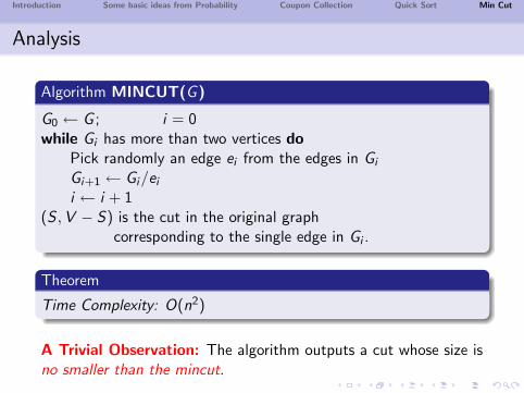
Algorithm MINCUT(G)
G0 ← G ; i = 0while Gi has more than two vertices do
Pick randomly an edge ei from the edges in Gi
Gi+1 ← Gi/ei
i ← i + 1(S ,V − S) is the cut in the original graph
corresponding to the single edge in Gi .
Theorem
Time Complexity: O(n2)
A Trivial Observation: The algorithm outputs a cut whose size isno smaller than the mincut.
Introduction Some basic ideas from Probability Coupon Collection Quick Sort Min Cut
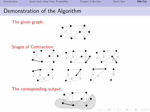
Demonstration of the Algorithm
The given graph:
Stages of Contraction:
2 2 22
2 2
2 2
3 2 3 2
4 45
9
The corresponding output:
Introduction Some basic ideas from Probability Coupon Collection Quick Sort Min Cut
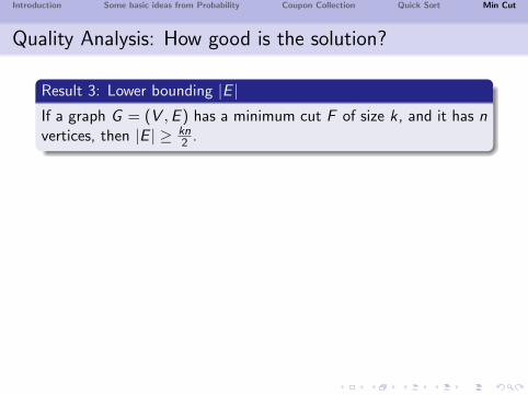
Quality Analysis: How good is the solution?
Result 3: Lower bounding |E |If a graph G = (V ,E ) has a minimum cut F of size k , and it has nvertices, then |E | ≥ kn
2 .
Proof
If any node v has degree less than k, then thecut({v},V − {v}) will have size less than k .
This contradicts the fact that (A,B) is a global min-cut.
Thus, every node in G has degree at least k . So, |E | ≥ 12kn.
So, the probability that an edge in F is contracted is at mostk
(kn)/2 = 2n
But, we don’t know the min cut.
Introduction Some basic ideas from Probability Coupon Collection Quick Sort Min Cut
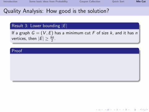
Quality Analysis: How good is the solution?
Result 3: Lower bounding |E |If a graph G = (V ,E ) has a minimum cut F of size k , and it has nvertices, then |E | ≥ kn
2 .
Proof
If any node v has degree less than k, then thecut({v},V − {v}) will have size less than k .
This contradicts the fact that (A,B) is a global min-cut.
Thus, every node in G has degree at least k . So, |E | ≥ 12kn.
So, the probability that an edge in F is contracted is at mostk
(kn)/2 = 2n
But, we don’t know the min cut.
Introduction Some basic ideas from Probability Coupon Collection Quick Sort Min Cut
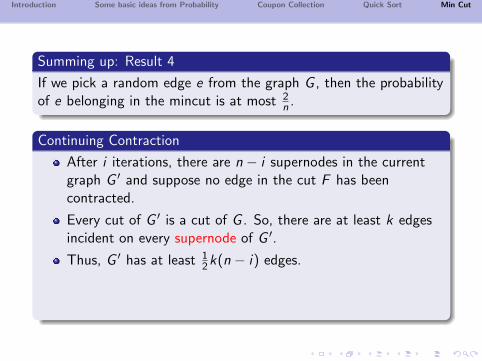
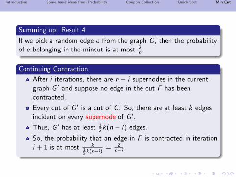
Summing up: Result 4
If we pick a random edge e from the graph G , then the probabilityof e belonging in the mincut is at most 2
n .
Continuing Contraction
After i iterations, there are n − i supernodes in the currentgraph G ′ and suppose no edge in the cut F has beencontracted.
Every cut of G ′ is a cut of G . So, there are at least k edgesincident on every supernode of G ′.
Thus, G ′ has at least 12k(n − i) edges.
So, the probability that an edge in F is contracted in iterationi + 1 is at most k
12k(n−i)
= 2n−i .
Introduction Some basic ideas from Probability Coupon Collection Quick Sort Min Cut
Correctness
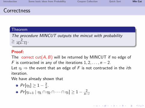
Theorem
The procedure MINCUT outputs the mincut with probability≥ 2
n(n−1) .
Proof:The correct cut(A,B) will be returned by MINCUT if no edge ofF is contracted in any of the iterations 1, 2, . . . , n − 2.Let ηi ⇒ the event that an edge of F is not contracted in the ithiteration.We have already shown that
Pr [η1] ≥ 1− 2n .
Pr [ηi+1 | η1 ∩ η2 ∩ · · · ∩ ηi ] ≥ 1− 2n−i
Introduction Some basic ideas from Probability Coupon Collection Quick Sort Min Cut
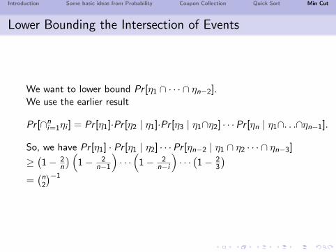
Lower Bounding the Intersection of Events
We want to lower bound Pr [η1 ∩ · · · ∩ ηn−2].We use the earlier result
Pr [∩ni=1ηi ] = Pr [η1]·Pr [η2 | η1]·Pr [η3 | η1∩η2] · · ·Pr [ηn | η1∩. . .∩ηn−1].
So, we have Pr [η1] · Pr [η1 | η2] · · ·Pr [ηn−2 | η1 ∩ η2 · · · ∩ ηn−3]
≥(1− 2
n
) (1− 2
n−1
)· · ·(
1− 2n−i
)· · ·(1− 2
3
)=(n2
)−1
Introduction Some basic ideas from Probability Coupon Collection Quick Sort Min Cut
Bounding the Error Probability
We know that a single run of the contraction algorithm failsto find a global min-cut with probability at most 1− 1
(n2)≈ 1.
We can amplify our success probability by repeatedly runningthe algorithm with independent random choices and takingthe best cut.
If we run the algorithm(n2
)times, then the probability that we
fail to find a global min-cut in any run is at most(1− 1(n
2
))(n2)
≤ 1
e.
Result
By spending O(n4) time, we can reduce the failure probabilityfrom 1− 2
n2 to a reasonably small constant value 1e .
Introduction Some basic ideas from Probability Coupon Collection Quick Sort Min Cut
Probability helps in counting
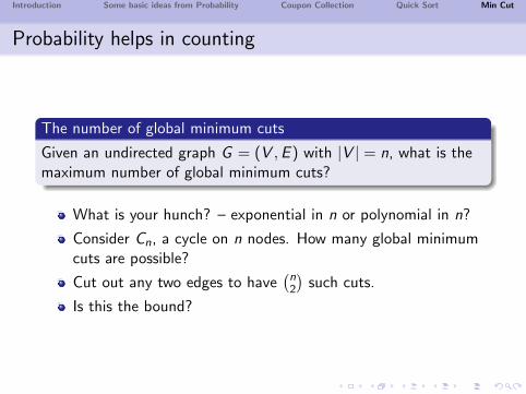
The number of global minimum cuts
Given an undirected graph G = (V ,E ) with |V | = n, what is themaximum number of global minimum cuts?
What is your hunch? – exponential in n or polynomial in n?
Consider Cn, a cycle on n nodes. How many global minimumcuts are possible?
Cut out any two edges to have(n2
)such cuts.
Is this the bound?
Introduction Some basic ideas from Probability Coupon Collection Quick Sort Min Cut
Probability helps in counting
The number of global minimum cuts
Given an undirected graph G = (V ,E ) with |V | = n, what is themaximum number of global minimum cuts?
What is your hunch? – exponential in n or polynomial in n?
Consider Cn, a cycle on n nodes. How many global minimumcuts are possible?
Cut out any two edges to have(n2
)such cuts.
Is this the bound?
Introduction Some basic ideas from Probability Coupon Collection Quick Sort Min Cut
The proof
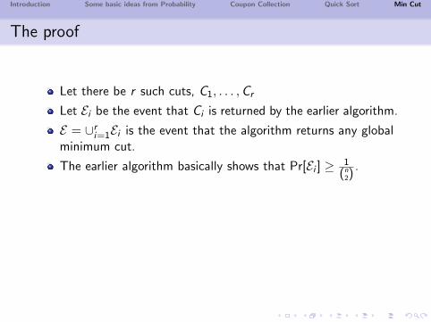
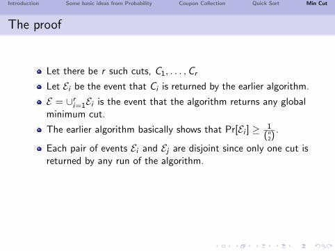
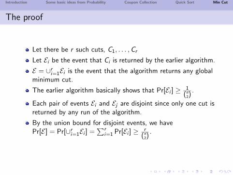
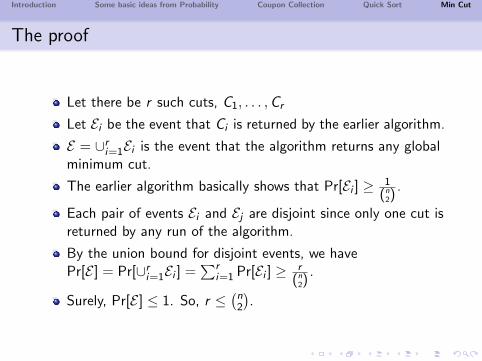
Let there be r such cuts, C1, . . . ,Cr
Let Ei be the event that Ci is returned by the earlier algorithm.
E = ∪ri=1Ei is the event that the algorithm returns any global
minimum cut.
The earlier algorithm basically shows that Pr[Ei ] ≥ 1
(n2)
.
Each pair of events Ei and Ej are disjoint since only one cut isreturned by any run of the algorithm.
By the union bound for disjoint events, we havePr[E ] = Pr[∪r
i=1Ei ] =∑r
i=1 Pr[Ei ] ≥ r
(n2)
.
Surely, Pr[E ] ≤ 1. So, r ≤(n2
).
Introduction Some basic ideas from Probability Coupon Collection Quick Sort Min Cut
The proof
Let there be r such cuts, C1, . . . ,Cr
Let Ei be the event that Ci is returned by the earlier algorithm.
E = ∪ri=1Ei is the event that the algorithm returns any global
minimum cut.
The earlier algorithm basically shows that Pr[Ei ] ≥ 1
(n2)
.
Each pair of events Ei and Ej are disjoint since only one cut isreturned by any run of the algorithm.
By the union bound for disjoint events, we havePr[E ] = Pr[∪r
i=1Ei ] =∑r
i=1 Pr[Ei ] ≥ r
(n2)
.
Surely, Pr[E ] ≤ 1. So, r ≤(n2
).
Introduction Some basic ideas from Probability Coupon Collection Quick Sort Min Cut
Conclusions
Employing randomness leads to improved simplicity andimproved efficiency in solving the problem.
It assumes the availability of a perfect source of independentand unbiased random bits.
Access to truly unbiased and independent sequence of randombits is expensive.So, it should be considered as an expensive resource like timeand space.
There are ways to reduce the randomness from severalalgorithms while maintaining the efficiency nearly the same.
Introduction Some basic ideas from Probability Coupon Collection Quick Sort Min Cut
Books
Jon Kleinberg and Eva Tardos, Algorithm Design, PearsonEducation.
Rajeev Motwani and Prabhakar Raghavan, RandomizedAlgorithms, Cambridge University Press, Cambridge, UK, 2004.
Michael Mitzenmacher and Eli Upfal, Probability andComputing: Randomized Algorithms and ProbabilisticAnalysis, Cambridge University Press, New York, USA, 2005..


