Download - Introduction to AlgorithmsGreedy Algorithms!Many optimization problems can be solved using a greedy approach "The basic principle is that local optimal decisions may may be used to

Introduction to Algorithms

Greedy Algorithms

Greedy Algorithms

! A greedy algorithm always makes the choice that looks best at the moment" The hope: a locally optimal choice will lead to a

globally optimal solution" For some problems, it works" My everyday examples:

# Walking to the Corner# Playing a bridge hand

! Dynamic programming can be overkill; greedy algorithms tend to be easier to code

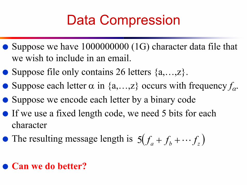
! Suppose we have 1000000000 (1G) character data file that we wish to include in an email.

! Suppose file only contains 26 letters {a,…,z}.! Suppose each letter a in {a,…,z} occurs with frequency fa.! Suppose we encode each letter by a binary code! If we use a fixed length code, we need 5 bits for each

character! The resulting message length is

! Can we do better?

Data Compression

( )zba fff !++5

Huffman Codes

! Most character code systems (ASCII, unicode) use fixed length encoding

! If frequency data is available and there is a wide variety of frequencies, variable length encoding can save 20% to 90% space

! Which characters should we assign shorter codes; which characters will have longer codes?

Data Compression: A Smaller Example

! Suppose the file only has 6 letters {a,b,c,d,e,f} with frequencies

! Fixed length 3G=3000000000 bits! Variable length

11001101111100101010110001101000100005.09.16.12.13.45.fedcba

Fixed length

Variable length

( ) G24.2405.409.316.312.313.145. =•+•+•+•+•+•

How to decode?

! At first it is not obvious how decoding will happen, but this is possible if we use prefix codes

Prefix Codes

! No encoding of a character can be the prefix of the longer encoding of another character, for example, we could not encode t as 01 and x as 01101 since 01 is a prefix of 01101

! By using a binary tree representation we will generate prefix codes provided all letters are leaves

Prefix codes

! A message can be decoded uniquely.

! Following the tree until it reaches to a leaf, and then repeat!

! Draw a few more tree and produce the codes!!!

! Prefix codes allow easy decoding" Given a: 0, b: 101, c: 100, d: 111, e: 1101, f: 1100" Decode 001011101 going left to right, 0|01011101, a|0|1011101,

a|a|101|1101, a|a|b|1101, a|a|b|e! An optimal code must be a full binary tree (a tree where every

internal node has two children)! For C leaves there are C-1 internal nodes! The number of bits to encode a file is

where f(c) is the freq of c, dT(c) is the tree depth of c, which corresponds to the code length of c

Some Properties

Optimal Prefix Coding Problem

! Input: Given a set of n letters (c1,…, cn) with frequencies (f1,…, fn).

! Construct a full binary tree T to define a prefix code that minimizes the average code length

( )iTn

i i cfT length )Average(1

•=å =

Greedy Algorithms

! Many optimization problems can be solved using a greedy approach" The basic principle is that local optimal decisions may

may be used to build an optimal solution" But the greedy approach may not always lead to an

optimal solution overall for all problems" The key is knowing which problems will work with

this approach and which will not! We will study

" The problem of generating Huffman codes

Greedy algorithms

! A greedy algorithm always makes the choice that looks best at the moment" My everyday examples:

# Playing cards# Invest on stocks# Choose a university

" The hope: a locally optimal choice will lead to a globally optimal solution

" For some problems, it works! Greedy algorithms tend to be easier to code

David Huffman’s idea

! Build the tree (code) bottom-up in a greedy fashion

Building the Encoding Tree

The Algorithm

! An appropriate data structure is a binary min-heap! Rebuilding the heap is lg n and n-1 extractions are

made, so the complexity is O( n lg n )! The encoding is NOT unique, other encoding may

work just as well, but none will work better

Correctness of Huffman’s Algorithm

Since each swap does not increase the cost, the resulting tree T’’ is also an optimal tree

Lemma 16.2

! Without loss of generality, assume f[a]£f[b] and f[x]£f[y]

! The cost difference between T and T’ is

0))()(])([][(

)(][)(][)(][)(][)(][)(][)(][)(][

)()()()()'()(

''

'

³--=

--+=--+=

å-å=-ÎÎ

xdadxfafxdafadxfadafxdxfadafxdxfadafxdxf

cdcfcdcfTBTB

TT

TTTT

TTTT

CcT

CcT

B(T’’) £ B(T), but T is optimal,

B(T) £ B(T’’) è B(T’’) = B(T)Therefore T’’ is an optimal tree in which x and y appear as sibling leaves of maximum depth

Correctness of Huffman’s Algorithm

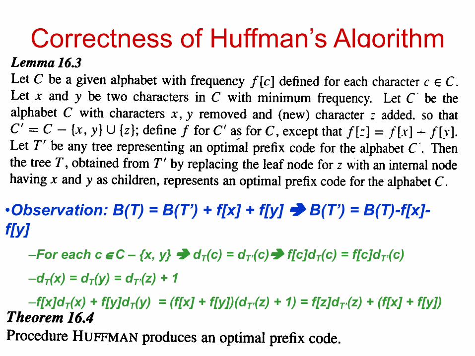
•Observation: B(T) = B(T’) + f[x] + f[y] è B(T’) = B(T)-f[x]-f[y]

–For each c ÎC – {x, y} è dT(c) = dT’(c)è f[c]dT(c) = f[c]dT’(c)

–dT(x) = dT(y) = dT’(z) + 1

–f[x]dT(x) + f[y]dT(y) = (f[x] + f[y])(dT’(z) + 1) = f[z]dT’(z) + (f[x] + f[y])

B(T’) = B(T)-f[x]-f[y]

B(T) = 45*1+12*3+13*3+5*4+9*4+16*3

z:14

B(T’) = 45*1+12*3+13*3+(5+9)*3+16*3= B(T) - 5 - 9

Proof of Lemma 16.3

! Prove by contradiction.! Suppose that T does not represent an optimal prefix code

for C. Then there exists a tree T’’ such that B(T’’) < B(T).! Without loss of generality, by Lemma 16.2, T’’ has x and

y as siblings. Let T’’’ be the tree T’’ with the common parent x and y replaced by a leaf with frequency f[z] = f[x] + f[y]. Then

! B(T’’’) = B(T’’) - f[x] – f[y] < B(T) – f[x] – f[y] = B(T’)" T’’’ is better than T’ è contradiction to the

assumption that T’ is an optimal prefix code for C’

Greedy algorithms

! A greedy algorithm always makes the choice that looks best at the moment" My everyday examples:

# Driving in Los Angeles, NY, or Boston for that matter# Playing cards# Invest on stocks# Choose a university

" The hope: a locally optimal choice will lead to a globally optimal solution

" For some problems, it works! greedy algorithms tend to be easier to code

! Input: A set of activities S = {a1,…, an}! Each activity has start time and a finish time

" ai=(si, fi)! Two activities are compatible if and only if

their interval does not overlap! Output: a maximum-size subset of

mutually compatible activities

An Activity Selection Problem(Conference Scheduling Problem)

Activity Selection: Optimal Substructure

!

Activity Selection:Repeated Subproblems

! Consider a recursive algorithm that tries all possible compatible subsets to find a maximal set, and notice repeated subproblems:

S1ÎA?

S’2ÎA?

S-{1}2ÎA?

S-{1,2}S’’S’-{2}S’’

yes no

nonoyes yes

Greedy Choice Property

! Dynamic programming? Memoize? Yes, but…! Activity selection problem also exhibits the

greedy choice property:" Locally optimal choice Þ globally optimal sol’n" Them 16.1: if S is an activity selection problem

sorted by finish time, then $ optimal solution A Í S such that {1} Î A# Sketch of proof: if $ optimal solution B that does not

contain {1}, can always replace first activity in B with {1} (Why?). Same number of activities, thus optimal.

The Activity Selection Problem

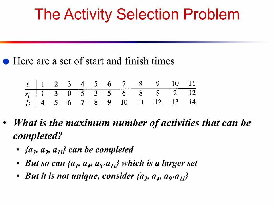
! Here are a set of start and finish times

• What is the maximum number of activities that can be completed?• {a3, a9, a11} can be completed• But so can {a1, a4, a8’ a11} which is a larger set• But it is not unique, consider {a2, a4, a9’ a11}

Interval Representation

0 1 2 3 4 5 6 7 8 9 10 11 12 13 14 15

Activity Selection: A Greedy Algorithm

! So actual algorithm is simple:" Sort the activities by finish time" Schedule the first activity" Then schedule the next activity in sorted list which

starts after previous activity finishes" Repeat until no more activities

! Intuition is even more simple:" Always pick the shortest ride available at the time

0 1 2 3 4 5 6 7 8 9 10 11 12 13 14 15

Assuming activities are sorted by finish time

Why it is Greedy?

! Greedy in the sense that it leaves as much opportunity as possible for the remaining activities to be scheduled

! The greedy choice is the one that maximizes the amount of unscheduled time remaining

Why this Algorithm is Optimal?

! We will show that this algorithm uses the following properties

! The problem has the optimal substructure property

! The algorithm satisfies the greedy-choice property

! Thus, it is Optimal

Greedy-Choice Property

! Show there is an optimal solution that begins with a greedy choice (with activity 1, which as the earliest finish time)

! Suppose A Í S in an optimal solution" Order the activities in A by finish time. The first activity in A is k

# If k = 1, the schedule A begins with a greedy choice# If k ¹ 1, show that there is an optimal solution B to S that begins with the

greedy choice, activity 1

" Let B = A – {k} È {1}# f1 £ fk à activities in B are disjoint (compatible)# B has the same number of activities as A# Thus, B is optimal

Optimal Substructures" Once the greedy choice of activity 1 is made, the problem

reduces to finding an optimal solution for the activity-selection problem over those activities in S that are compatible with activity 1# Optimal Substructure# If A is optimal to S, then A’ = A – {1} is optimal to S’={i ÎS: si ³ f1}# Why?

$ If we could find a solution B’ to S’ with more activities than A’, adding activity 1 to B’ would yield a solution B to S with more activities than A è contradicting the optimality of A

" After each greedy choice is made, we are left with an optimization problem of the same form as the original problem# By induction on the number of choices made, making the greedy

choice at every step produces an optimal solution

Elements of Greedy Strategy

! An greedy algorithm makes a sequence of choices, each of the choices that seems best at the moment is chosen" NOT always produce an optimal solution

! Two ingredients that are exhibited by most problems that lend themselves to a greedy strategy" Greedy-choice property" Optimal substructure

Greedy-Choice Property

! A globally optimal solution can be arrived at by making a locally optimal (greedy) choice" Make whatever choice seems best at the moment and

then solve the sub-problem arising after the choice is made

" The choice made by a greedy algorithm may depend on choices so far, but it cannot depend on any future choices or on the solutions to sub-problems

! Of course, we must prove that a greedy choice at each step yields a globally optimal solution

Optimal Substructures

! A problem exhibits optimal substructure if an optimal solution to the problem contains within it optimal solutions to sub-problems" If an optimal solution A to S begins with activity

1, then A’ = A – {1} is optimal to S’={i ÎS: si ³f1}

Greedy Vs. Dynamic Programming:The Knapsack Problem

! The famous knapsack problem:" A thief breaks into a museum. Fabulous paintings,

sculptures, and jewels are everywhere. The thief has a good eye for the value of these objects, and knows that each will fetch hundreds or thousands of dollars on the clandestine art collector’s market. But, the thief has only brought a single knapsack to the scene of the robbery, and can take away only what he can carry. What items should the thief take to maximize the haul?

The Knapsack Problem

! More formally, the 0-1 knapsack problem:" The thief must choose among n items, where the

ith item worth vi dollars and weighs wi pounds" Carrying at most W pounds, maximize value

# Note: assume vi, wi, and W are all integers# “0-1” b/c each item must be taken or left in entirety

! A variation, the fractional knapsack problem:" Thief can take fractions of items" Think of items in 0-1 problem as gold ingots, in

fractional problem as buckets of gold dust

The Knapsack Problem: Optimal Substructure

! Both variations exhibit optimal substructure! To show this for the 0-1 problem, consider the

most valuable load weighing at most W pounds" If we remove item j from the load, what do we

know about the remaining load?" A: remainder must be the most valuable load

weighing at most W - wj that thief could take from museum, excluding item j

Solving The Knapsack Problem

! The optimal solution to the fractional knapsack problem can be found with a greedy algorithm" How?

! The optimal solution to the 0-1 problem cannot be found with the same greedy strategy" Greedy strategy: take in order of dollars/pound" Example: 3 items weighing 10, 20, and 30 pounds,

knapsack can hold 50 pounds# Suppose item 2 is worth $100. Assign values to the

other items so that the greedy strategy will fail

The Knapsack Problem: Greedy Vs. Dynamic

! The fractional problem can be solved greedily! The 0-1 problem cannot be solved with a

greedy approach" It can, however, be solved with dynamic

programming

Download - Introduction to AlgorithmsGreedy Algorithms!Many optimization problems can be solved using a greedy approach "The basic principle is that local optimal decisions may may be used to

Top Related