INTERMODAL TRANSPORTATION OF HAZARDOUS
MATERIALS WITH SUPPLIER SELECTION: APPLICATION IN TURKEY
A THESIS
SUBMITTED TO THE DEPARTMENT OF INDUSTRIAL
ENGINEERING
AND THE GRADUATE SCHOOL OF ENGINEERING AND SCIENCE OF
BILKENT UNIVERSITY
IN PARTIAL FULFILLMENT OF THE REQUIREMENTS
FOR THE DEGREE OF
MASTER OF SCIENCE
by
Pelin Elaldı
November 2011
ii
I certify that I have read this thesis and that in my opinion it is full adequate, in scope
and in quality, as a dissertation for the degree of Master of Science.
___________________________________
Assoc. Prof. Bahar Y. Kara (Advisor)
I certify that I have read this thesis and that in my opinion it is full adequate, in scope
and in quality, as a dissertation for the degree of Master of Science.
___________________________________
Asst. Prof. Osman Alp (Co-Advisor)
I certify that I have read this thesis and that in my opinion it is full adequate, in scope
and in quality, as a dissertation for the degree of Master of Science.
______________________________________
Asst. Prof. Alper ġen
I certify that I have read this thesis and that in my opinion it is full adequate, in scope
and in quality, as a dissertation for the degree of Master of Science.
______________________________________
Asst. Prof. Sibel Alumur Alev
Approved for the Graduate School of Engineering and Science
____________________________________
Prof. Dr. Levent Onural
Director of the Graduate School of Engineering and Science
iii
ABSTRACT
INTERMODAL TRANSPORTATION OF HAZARDOUS
MATERIALS WITH SUPPLIER SELECTION: APPLICATION IN TURKEY
Pelin Elaldı
M.S. in Industrial Engineering
Supervisor: Assoc. Prof. Bahar Y. Kara
Co-Supervisor: Assist. Prof. Osman Alp
November 2011
Fuel transportation constitutes a significant portion of hazardous materials transportation
for decades. Fuel companies generally prefer highway transportation whereas railway
transportation is also a potential alternative due to its advantages both from cost- and
risk perspectives. The aim of this thesis is to investigate the potential benefits of using
railways in conjunction to highways for fuel transportation in Turkey. In this thesis, we
first investigate a quantitative risk model that could be used to assess the risk of railway
transportation. Then, a mathematical model is developed which aims to answer the
following three questions: What should be the routes of fuel products transported from
suppliers to demand points and which transportation mode(s) should be used on these
routes?, Where to open transfer units?, and Which suppliers should satisfy which
demand points with what capacity?. The model has two possibly conflicting objectives
of minimizing the total transportation risk and minimizing the total transportation cost.
The proposed models are tested over Turkish network for which all required realistic
data are collected.
Keywords: Hazardous Materials Transportation, Intermodal Transportation, Risk
Analysis
iv
ÖZET
TEHLĠKELĠ MADDE TAġIMACILIĞINDA TEDARĠKÇĠ SEÇĠMĠ VE ÇOK MOD
KULLANIMI: TÜRKĠYE ÜZERĠNDE UYGULAMA
Pelin Elaldı
Endüstri Mühendisliği Yüksek Lisans
Tez Yöneticisi: Doç Dr. Bahar Y. Kara
EĢ-Tez Yöneticisi: Yrd. Doç. Dr. Osman Alp
Kasım 2011
Akaryakıt taĢımacılığı yıllardır tehlikeli madde taĢımacılığının önemli bir bölümünü
oluĢturmaktadır. Demiryolu ile taĢımacılık risk ve maliyet açılarından avantajlı bir
alternatif olsa da akaryakıt firmaları genellikle ürünlerini karayolu ile taĢımaktadır. Bu
çalıĢmanın amacı, akaryakıt taĢımacılığında demiryollarının karayolları ile birlikte
kullanımın oluĢturacağı potansiyel faydaları araĢtırmaktır. Bu çalıĢmada, öncelikle
demiryolu taĢımacılığı riskini belirleyebilmek için kullanılabilecek nicel
bir risk modeli araĢtırılmıĢtır. Daha sonra Ģu üç soruya cevap vermesi amaçlanan bir
matematiksel model geliĢtirilmiĢtir: Akaryakıt ürünleri tedarikçilerden talep noktalarına
kadar hangi rotaları izlemeli ve bu rotalar üzerinde hangi ulaĢtırma modu/ modları
kullanılmalı? Nerelere transfer ünitesi açılmalı? ve Hangi tedarikçiler hangi talep
noktalarının taleplerini hangi kapasite ile karĢılamalı? Modelin biri taĢıma riskinin
enküçüklenmesi, diğeri taĢıma maliyetini enküçüklenmesi olmak üzere iki tane amacı
vardır. Sunulan modeller, elde edilebilecek bütün gerçekçi veriler toplanarak Türkiye ağı
üzerinde test edilmiĢtir.
Anahtar Kelimeler: Tehlikeli Madde TaĢımacılığı, Birden Fazla UlaĢtırma Modu
ile TaĢımacılık, Risk Analizi

v
ACKNOWLEDGEMENT
I would like to express my sincere gratitude to Assoc. Prof. Bahar Y. Kara and Assist.
Prof. Osman Alp for their invaluable guidance and support during my graduate study.
They have supervised me with everlasting patience and encouragement throughout this
thesis. I consider myself lucky to have a chance to work with them.
I am also grateful to Asst. Prof. Alper ġen and Asst. Prof. Sibel Alumur Alev for
accepting to read and review this thesis. Their comments and suggestions have been
invaluable.
I also would like to express my deepest gratitude to my family for their eternal love,
support and trust at all stages of my life and especially during my graduate study. I feel
very lucky that I belong to this family.
I am indeed grateful to Doruk Özdemir for his morale support, patience, encouragement
and endless love since I met him.
I would like to thank to my precious friends Müge Muhafız, Fevzi Yılmaz, Nurcan
Bozkaya, and Onur Uzunlar for their endless support, motivation and wholehearted love.
Life and the graduate study would not have been bearable without them. I also would
like to thank my cousin Özge Aksoy and my dear friend Zeynep ġagar for their
friendship and support.
Finally, I would like to acknowledged financial support of The Scientific and
Technological Research Council of Turkey (TUBITAK) for the Graduate Study
Scholarship Program.
vi
TABLE OF CONTENTS
Chapter 1 ............................................................................................................................ 1
Introduction .................................................................................................................... 1
Chapter 2 ............................................................................................................................ 4
Fuel Transportation in Turkey ........................................................................................ 4
Chapter 3 .......................................................................................................................... 14
Problem Definition ....................................................................................................... 14
Chapter 4 .......................................................................................................................... 23
Literature Review ......................................................................................................... 23
4.1. Hazardous Materials Transportation .................................................................. 23
4.2. Intermodal Transportation ................................................................................. 29
4.3. Intermodal Transportation of Hazardous Materials ........................................... 35
Chapter 5 .......................................................................................................................... 38
Model Development ..................................................................................................... 38
5.1. Transportation Risk Model ................................................................................ 38
5.2. Mathematical Model .......................................................................................... 43
Chapter 6 .......................................................................................................................... 50
Data Collection and Computational Results................................................................. 50
6.1. Data Collection .................................................................................................. 51
6.2. Numerical Analysis............................................................................................ 59
Chapter 7 .......................................................................................................................... 77
Conclusion .................................................................................................................... 77
BIBLIOGRAPHY ............................................................................................................ 81
APPENDIX ...................................................................................................................... 85

vii
LIST OF FIGURES
Figure 2.1 Fuel Consumption in Turkey ............................................................................ 5
Figure 2.2-Market Shares of Fuel Distribution Companies in Turkey .............................. 6
Figure 2.3 Fuel Procurement Ways .................................................................................... 8
Figure 2.4 Terminals of Petrol Ofisi ................................................................................ 11
Figure 2.5 Distribution System Using Transfer Units ..................................................... 12
Figure 3.1 Factors Caused to Hazmat Accidents Based on Transportation Modes ......... 16
Figure 3.2 Current Fuel Distribution System in Turkey .................................................. 18
Figure 3.3- a, b, c, d-Intermodal Transportation, e-Highway Transportation, f-Railway
Transportation .................................................................................................................. 20
Figure 4.1 Shapes of Impact Area Around the Route Segment ....................................... 25
Figure 4.2 Summary of the Five Risk Models Suggested in the Literature for Hazmat
Transport Risk, Source: Erkut and Verter (1998) ............................................................ 26
Figure 4.3 Rail-Truck Intermodal Transportation, Source: Macharis and Bontekoning
(2004) ............................................................................................................................... 30
Figure 4.4 Rail-Truck Intermodal Transportation Characteristics, Source: Bontekoning
et al (2004) ....................................................................................................................... 30
Figure 4.5 Differences of Rail Transportation, Source: Bontekoning et al. (2004) ......... 33
Figure 6.1 Annual Sales of Cities (EMRA, 2010) ........................................................... 54
Figure 6.2- Highway Network ......................................................................................... 56
Figure 6.3- Railway Network ........................................................................................... 57
Figure 6.4- Final Railway-Highway Network ................................................................. 57
Figure 6.5- Impact Area- Fixed Bandwidth ..................................................................... 58
Figure 6.6- Derailment Probability Distribution .............................................................. 59
Figure 6.7- MC and MR Solutions of SMS and IMS ...................................................... 63
viii
Figure 6.8- Percentage Distributions of MC and MR Solutions of Single Mode
Alternative ........................................................................................................................ 64
Figure 6.9- Percentage Distributions of MC and MR Solutions of Intermodal Alternative
.......................................................................................................................................... 65
Figure 6.10- Trade-Off Curve for IMS Alternative ......................................................... 67
Figure 6.11- Trade-off Curve for IMSL Alternative ........................................................ 68
Figure 6.12- Effects of Opening Different Number of Transfer Units ............................ 70
Figure 6.13- Percentage Usage of Railways in Different k Values When Solving MR-
βCost Model where β equals to MC(SMS) value ............................................................ 73
Figure 6.14 Bandwidths Around the Railway and Highway Arcs of Kayseri-Sivas Pair 74
Figure 6.15- Solutions Obtained for Different k values ................................................... 75
Figure 6.16 Percentage Usage Of Railways in Different k Values When Solving MR
Model ............................................................................................................................... 76
ix
LIST OF TABLES
Table 2-1 Capacities of Refineries ..................................................................................... 8
Table 5-1 Notations Used in Railway Risk Model .......................................................... 40
Table 6-1 Data Components ............................................................................................ 51
Table 6-2- Selected Supply Points ................................................................................... 52
Table 6-3- Fixed Storage Terminals ................................................................................ 52
Table 6-4- Selected Transfer Units .................................................................................. 53
Table 6-5- MC and MR Results of Alternatives .............................................................. 61
Table 6-6- MC and MR Results of IMSL5 and IMSL7 Alternatives ................................. 66
Table 6-7- MC and MR Solutions when k=0.8 and k=0.7 ............................................... 72
1
Chapter 1
Introduction
A hazardous material (hazmat) can be defined as any material that could harm people,
property or the environment. Hazmats include explosive and pyrotechnics, gasses,
flammable and combustible liquids, flammable-combustible and dangerous-when-wet
solids, oxidizers and organic peroxides, poisonous and infectious materials, radioactive
materials, corrosive materials (acidic or basic), and hazardous wastes. The source of
hazardous materials can be industrial and chemical plants, petroleum refineries, medical
stations such as hospitals and clinics. Some possible accidents/incidents that impose risk
to people, property and the environment could be an explosion in storage or processing
facilities, leak of hazmats from their containers directly to the atmosphere, or an
explosion or a leak due to a traffic accident involving hazmat-carrying vehicles.
Consequently, such incidents might have catastrophic consequences. Hence,
transportation of these materials should be handled with extreme care.
2
In this study, we focus on the transportation of fuel products. Fuel products belong to the
class of flammable-combustible liquids. In the current fuel distribution system of
Turkey, fuel transportation is materialized by using highways. An alternative to
highways is railroad transportation. Even though Turkey has a sparse railroad network,
railroad alternative could be a preferred alternative over highways as the transportation
cost and risk of railways could be lower than those of the highways. Thus, a combination
of railway and highway transportation alternatives should be considered together. This
type of transportation is referred as “intermodal transportation” in the literature.
In the literature, there are number of studies that deal with measuring highway
transportation risk of hazardous materials. However, there are just a few studies that
focus on railway transportation risk. In this study, we adapt the risk model conducted by
Glickman et al. (2007) and modify the model to our case by making a few changes. We
collected all the required data specialized on Turkey as realistic as possible.
Due to the nature of products being transported, societal risk should also be considered
as a performance measure as transportation cost. Therefore, this problem has multiple
and possibly conflicting objectives and priority of these performance measures may
differ among the perspectives. Thus, the aim of this thesis is to find routes between
supply points and demand points on a given network composed of highways and
railways; and locate the transshipment points on that network, so that selected risk
and/or cost measures are optimized in an appropriate manner.
In the next chapter, we explain the current fuel distribution system of Turkey. Fuel
companies, fuel consumption in Turkey and the main steps of fuel distribution system
are the main topics of this chapter. In Chapter 3, we define the problem considered in
this study by presenting its structure and parameters. In Chapter 4, the related literature
is examined in three main parts, which are hazardous materials transportation,
intermodal transportation, and intermodal transportation of hazardous materials. In
3
Chapter 5, we introduce a transportation risk model for highway and railway
transportation and a mathematical model to obtain efficient solutions for the problem
defined in Chapter 3. We discuss the analyses and the computational results of the given
model in Chapter 6 and finally in Chapter 7, we conclude the thesis by briefly
summarizing our efforts and contributions of the thesis.
4
Chapter 2
Fuel Transportation in Turkey
Petroleum products are the outputs of the distillation of crude oil under different heat
and pressure. Basically, there are three main product groups;
White products: Automotive fuels, coal oil, aircraft fuel
Black Products: Fuel oil and heating oil
Oils: engine oil, industrial oil
Automotive fuel consumption is continuously increasing every year in Turkey.
According to PETDER (2010), total consumption of the white products (Gasoline, diesel
fuels and LPG auto-gas) increased by 1.9% since 2009 and reach to 18.4 million tons in
2010 (See Figure 2.1).
5
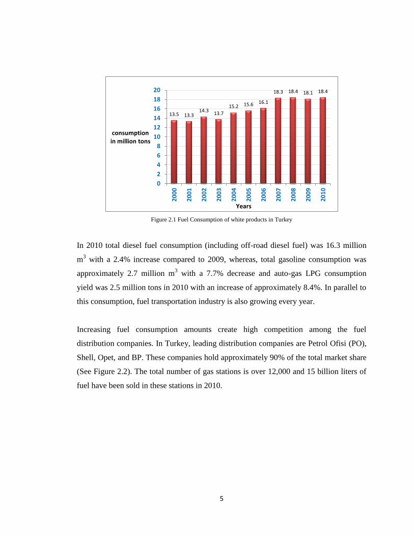
Figure 2.1 Fuel Consumption of white products in Turkey
In 2010 total diesel fuel consumption (including off-road diesel fuel) was 16.3 million
m3 with a 2.4% increase compared to 2009, whereas, total gasoline consumption was
approximately 2.7 million m3 with a 7.7% decrease and auto-gas LPG consumption
yield was 2.5 million tons in 2010 with an increase of approximately 8.4%. In parallel to
this consumption, fuel transportation industry is also growing every year.
Increasing fuel consumption amounts create high competition among the fuel
distribution companies. In Turkey, leading distribution companies are Petrol Ofisi (PO),
Shell, Opet, and BP. These companies hold approximately 90% of the total market share
(See Figure 2.2). The total number of gas stations is over 12,000 and 15 billion liters of
fuel have been sold in these stations in 2010.
13.5 13.3 14.3
13.7
15.2 15.6 16.1
18.3 18.4 18.1 18.4
0
2
4
6
8
10
12
14
16
18
20
20
00
20
01
20
02
20
03
20
04
20
05
20
06
20
07
20
08
20
09
20
10
consumption in million tons
Years
6
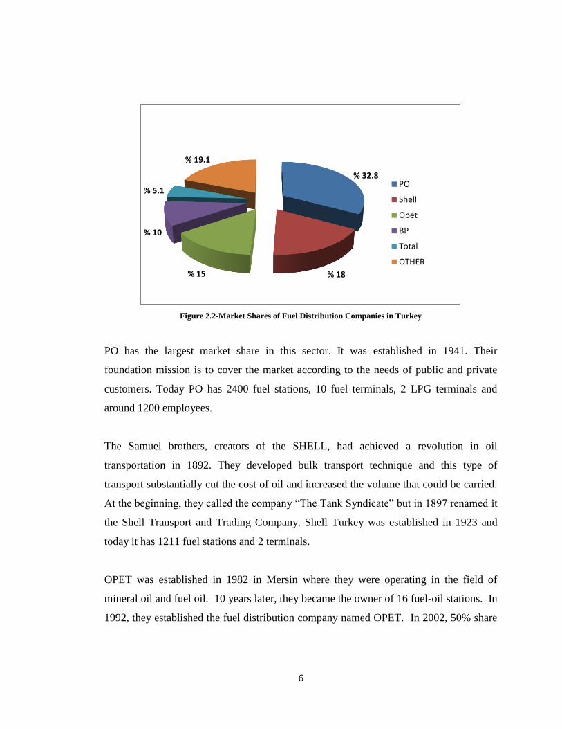
Figure 2.2-Market Shares of Fuel Distribution Companies in Turkey
PO has the largest market share in this sector. It was established in 1941. Their
foundation mission is to cover the market according to the needs of public and private
customers. Today PO has 2400 fuel stations, 10 fuel terminals, 2 LPG terminals and
around 1200 employees.
The Samuel brothers, creators of the SHELL, had achieved a revolution in oil
transportation in 1892. They developed bulk transport technique and this type of
transport substantially cut the cost of oil and increased the volume that could be carried.
At the beginning, they called the company “The Tank Syndicate” but in 1897 renamed it
the Shell Transport and Trading Company. Shell Turkey was established in 1923 and
today it has 1211 fuel stations and 2 terminals.
OPET was established in 1982 in Mersin where they were operating in the field of
mineral oil and fuel oil. 10 years later, they became the owner of 16 fuel-oil stations. In
1992, they established the fuel distribution company named OPET. In 2002, 50% share
% 32.8
% 18 % 15
% 10
% 5.1
% 19.1
PO
Shell
Opet
BP
Total
OTHER
7
of the company was owned by Koç Holding Energy Group. Now, OPET has 1258 fuel
stations and 6 terminals.
BP is the fourth biggest company in the market. The company was established in 1908
and penetrated into the Turkish market in 1949. First year, sales amount was 40,000
tones and reached to 200,000 tons in 1961. Today, BP has 630 fuel stations and 130
LPG terminals.
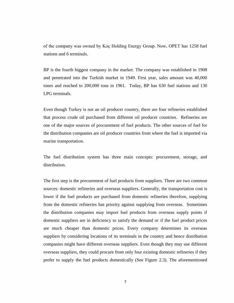
Even though Turkey is not an oil producer country, there are four refineries established
that process crude oil purchased from different oil producer countries. Refineries are
one of the major sources of procurement of fuel products. The other sources of fuel for
the distribution companies are oil producer countries from where the fuel is imported via
marine transportation.
The fuel distribution system has three main concepts: procurement, storage, and
distribution.
The first step is the procurement of fuel products from suppliers. There are two common
sources: domestic refineries and overseas suppliers. Generally, the transportation cost is
lower if the fuel products are purchased from domestic refineries therefore, supplying
from the domestic refineries has priority against supplying from overseas. Sometimes
the distribution companies may import fuel products from overseas supply points if
domestic suppliers are in deficiency to satisfy the demand or if the fuel product prices
are much cheaper than domestic prices. Every company determines its overseas
suppliers by considering locations of its terminals in the country and hence distribution
companies might have different overseas suppliers. Even though they may use different
overseas suppliers, they could procure from only four existing domestic refineries if they
prefer to supply the fuel products domestically (See Figure 2.3). The aforementioned
8
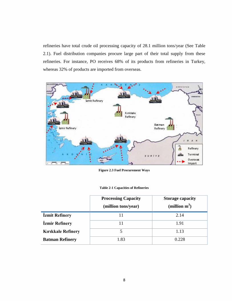
refineries have total crude oil processing capacity of 28.1 million tons/year (See Table
2.1). Fuel distribution companies procure large part of their total supply from these
refineries. For instance, PO receives 68% of its products from refineries in Turkey,
whereas 32% of products are imported from overseas.
Figure 2.3 Fuel Procurement Ways
Table 2-1 Capacities of Refineries
Processing Capacity
(million tons/year)
Storage capacity
(million m3)
İzmit Refinery 11 2.14
İzmir Refinery 11 1.91
Kırıkkale Refinery 5 1.13
Batman Refinery 1.83 0.228
9
The Ġzmit Refinery started production in 1961, with a 1 million tons/year capacity of
crude oil processing. The next 20 years, its processing capacity reached to 11 million
tons/year through investments. Main products produced in the refinery are LPG,
naphtha, gasoline, jet fuel, kerosene, diesel, heating oil, fuel oil, and asphalt. In 2010,
Ġzmit Refinery processed 8.5 million tons of crude oil.
To meet the growing demand of petroleum products, in 1972 the Ġzmir Refinery has
been established and started production. The initial crude oil processing capacity was 3
million tons/year. Up till 1987, with the capacity augmentations, its capacity reached to
10 million tons/year and today it has 11 million tons/year processing capacity. Main
products are LPG, naphtha, gasoline, jet fuel, diesel, base oil, heating oil, fuel oil,
asphalt, wax, extracts and other products. Ġzmir Refinery processed 8.5 million tons in
2010.
Kırıkkale Refinery was established to meet the growing demand in the Central
Anatolian, Eastern Mediterranean and Eastern Black Sea Regions in 1986. Its
processing capacity is 5 million tons/year whereas capacity utilization for crude oil is
53%. Main products are LPG, gasoline, jet fuel, kerosene, diesel, fuel oil, and asphalt. In
2010, this refinery produced 2.7 million tons of petroleum products.
Batman Refinery is the first refinery established in Turkey. It started production in 1955
with a capacity of 330 thousand tons. Up to 1972, its crude oil processing capacity
reached to 1.1 million tons/year. Main products produced in refinery are asphalt,
naphtha, diesel and semi-finished products. In 2010, the refinery processed 903,000 tons
of crude oil.
10
The second step is to store the fuel products procured from overseas suppliers or
refineries. Storage of the petroleum products has a significant importance on the
distribution. Companies can establish their own storage terminals as well as they can use
other companies’ terminals. These terminals provide safe storage of the fuel products on
the land. Some of these terminals are nearby the refineries in Turkey. On the other hand,
some of them are located in the coastal areas (Aegean, Mediterranean and Black Sea)
where there are several active seaports available. No matter where they procure the fuel
products, companies store them safely in the depots in the storage terminals.
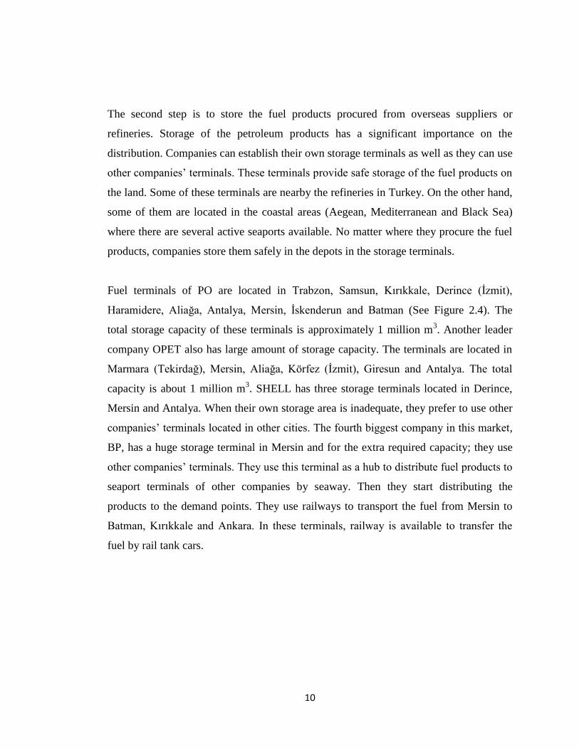
Fuel terminals of PO are located in Trabzon, Samsun, Kırıkkale, Derince (Ġzmit),
Haramidere, Aliağa, Antalya, Mersin, Ġskenderun and Batman (See Figure 2.4). The
total storage capacity of these terminals is approximately 1 million m3. Another leader
company OPET also has large amount of storage capacity. The terminals are located in
Marmara (Tekirdağ), Mersin, Aliağa, Körfez (Ġzmit), Giresun and Antalya. The total
capacity is about 1 million m3. SHELL has three storage terminals located in Derince,
Mersin and Antalya. When their own storage area is inadequate, they prefer to use other
companies’ terminals located in other cities. The fourth biggest company in this market,
BP, has a huge storage terminal in Mersin and for the extra required capacity; they use
other companies’ terminals. They use this terminal as a hub to distribute fuel products to
seaport terminals of other companies by seaway. Then they start distributing the
products to the demand points. They use railways to transport the fuel from Mersin to
Batman, Kırıkkale and Ankara. In these terminals, railway is available to transfer the
fuel by rail tank cars.
11
Figure 2.4 Terminals of Petrol Ofisi
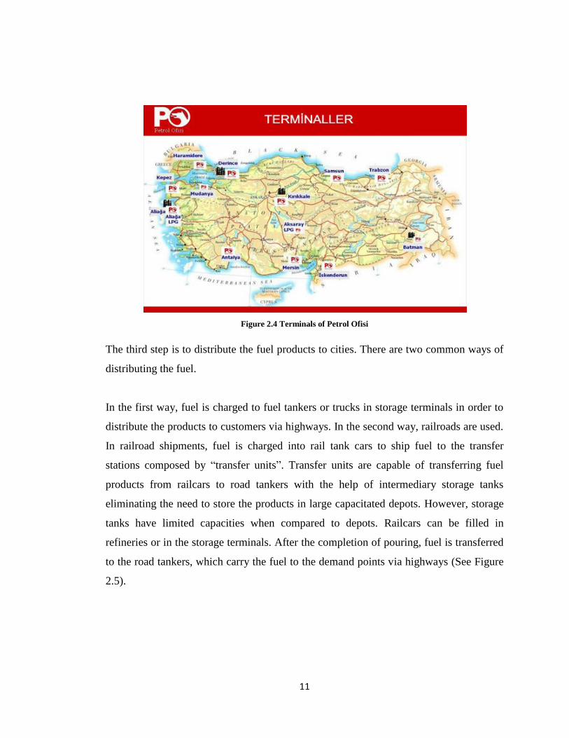
The third step is to distribute the fuel products to cities. There are two common ways of
distributing the fuel.
In the first way, fuel is charged to fuel tankers or trucks in storage terminals in order to
distribute the products to customers via highways. In the second way, railroads are used.
In railroad shipments, fuel is charged into rail tank cars to ship fuel to the transfer
stations composed by “transfer units”. Transfer units are capable of transferring fuel
products from railcars to road tankers with the help of intermediary storage tanks
eliminating the need to store the products in large capacitated depots. However, storage
tanks have limited capacities when compared to depots. Railcars can be filled in
refineries or in the storage terminals. After the completion of pouring, fuel is transferred
to the road tankers, which carry the fuel to the demand points via highways (See Figure
2.5).
12
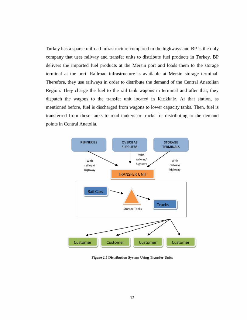
Turkey has a sparse railroad infrastructure compared to the highways and BP is the only
company that uses railway and transfer units to distribute fuel products in Turkey. BP
delivers the imported fuel products at the Mersin port and loads them to the storage
terminal at the port. Railroad infrastructure is available at Mersin storage terminal.
Therefore, they use railways in order to distribute the demand of the Central Anatolian
Region. They charge the fuel to the rail tank wagons in terminal and after that, they
dispatch the wagons to the transfer unit located in Kırıkkale. At that station, as
mentioned before, fuel is discharged from wagons to lower capacity tanks. Then, fuel is
transferred from these tanks to road tankers or trucks for distributing to the demand
points in Central Anatolia.
Figure 2.5 Distribution System Using Transfer Units
REFINERIES OVERSEAS SUPPLIERS
STORAGE TERMINALS
With
railway/
highway
Rail Cars
Trucks
TRANSFER UNIT
With
railway/
highway With
railway/
highway
Customer Customer Customer Customer
Storage Tanks
13
To sum up, fuel distribution is composed of three main steps. Firstly, fuel is procured
from refineries or overseas suppliers. In the second step, fuel is stored at the depots in
the storage terminals. At the final step, fuel is distributed to customers by using only
highways or using highways together with railways. In this step, from the leader
companies of the fuel distribution sector, Petrol Ofisi, Shell and Opet uses only
highways whereas BP uses both railways and highways while distributing the fuel
products
14
Chapter 3
Problem Definition
A hazardous material (hazmat) is defined as any substance or material capable of
causing harm to people, property and the environment (US Department of
Transportation). Basically, there are nine main classes of hazardous materials;
1. Explosive and pyrotechnics
2. Gasses
3. Flammable and combustible liquids
4. Flammable, combustible and dangerous-when-wet solids
5. Oxidizers and organic peroxides
6. Poisonous and infectious materials
7. Radioactive materials
8. Corrosive materials (acidic or basic)
9. Miscellaneous dangerous goods (hazardous wastes)
15
Among these classes flammable-combustible liquids (48.44%) and corrosive materials
(25%) generates the major volume of the hazmat accidents/incidents (U.S. Department
of Transportation, 2011) and white/black fuel products belong to this class of hazardous
materials. Some possible accidents/incidents that impose risk to people, property and the
environment could be an explosion in storage or processing facilities, leak of hazmats
from their containers directly to the atmosphere, or an explosion or a leak due to a traffic
accident involving hazmat-carrying vehicles. Obviously, such incidents might have
catastrophic consequences. Consequently, storing, processing and transportation of
hazmats must be handled with extreme care and attention by the authorities so that the
risk imposed to the society and environment is minimized as much as possible. In this
thesis, we are focusing on the transportation operations of hazmats and the
corresponding risk imposed on the society.
Since the transportation of hazardous materials imposes risk to the public and
environment, it is essential to measure the risk by appropriate measures. An example is
the “traditional risk” measure, which is obtained by multiplying the probability of the
occurrence of an undesired event (e.g. a traffic accident) and its corresponding
consequence. Another example of a risk measure could be population exposure, which is
the total number of people exposed to risk during the transportation of a hazmat carrying
vehicle.
Hazardous materials could be transported via five modes: road, rail, water, air, and
pipeline. Among these modes, the great majority move by rail and truck. While 94% of
all hazmat shipments are done by trucks that many shipments account for 43% of the
total transported hazmat tonnage. Carrying hazmat with rail, water, and pipelines
account for 57% of the total hazmat tonnage, while they hold only 1% of total hazmat
shipments in 2004 in USA (Erkut et al., 2007).
16
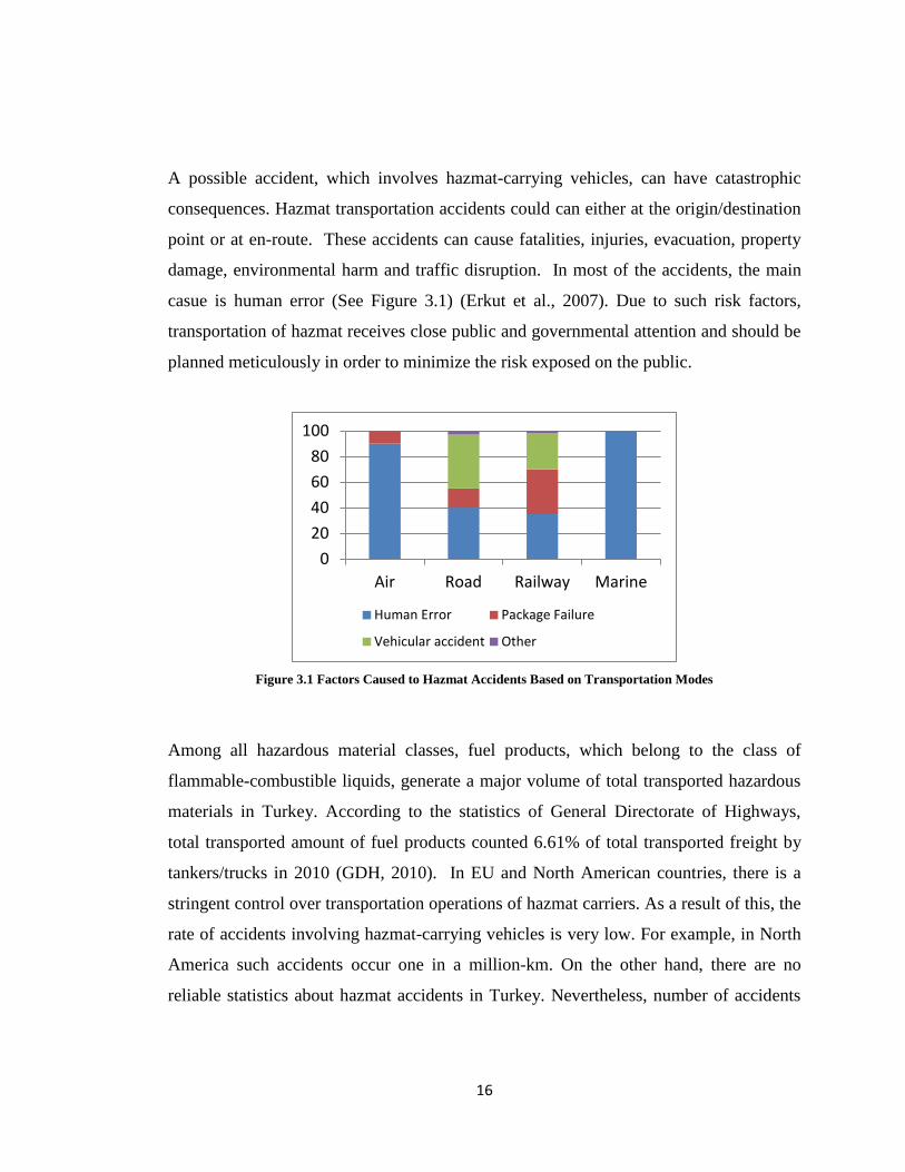
A possible accident, which involves hazmat-carrying vehicles, can have catastrophic
consequences. Hazmat transportation accidents could can either at the origin/destination
point or at en-route. These accidents can cause fatalities, injuries, evacuation, property
damage, environmental harm and traffic disruption. In most of the accidents, the main
casue is human error (See Figure 3.1) (Erkut et al., 2007). Due to such risk factors,
transportation of hazmat receives close public and governmental attention and should be
planned meticulously in order to minimize the risk exposed on the public.
Figure 3.1 Factors Caused to Hazmat Accidents Based on Transportation Modes
Among all hazardous material classes, fuel products, which belong to the class of
flammable-combustible liquids, generate a major volume of total transported hazardous
materials in Turkey. According to the statistics of General Directorate of Highways,
total transported amount of fuel products counted 6.61% of total transported freight by
tankers/trucks in 2010 (GDH, 2010). In EU and North American countries, there is a
stringent control over transportation operations of hazmat carriers. As a result of this, the
rate of accidents involving hazmat-carrying vehicles is very low. For example, in North
America such accidents occur one in a million-km. On the other hand, there are no
reliable statistics about hazmat accidents in Turkey. Nevertheless, number of accidents
0
20
40
60
80
100
Air Road Railway Marine
Human Error Package Failure
Vehicular accident Other
17
occurring on Turkey’s highways is significantly higher when compared to the EU and
North American countries. To give some statistics, there were 11,119 accidents
involving trucks or tankers in Turkey in 2010 whereas number of total accidents was
1,106,201 (TSI, 2010). However, total number of Motor Vehicle Traffic accidents is
30,797 in USA in 2009 according to the NHTSA (2009). In addition, the number of
vehicles that carry fuel products counted 4% of total traveled vehicle along the highways
in 2010. Therefore, planning for better transportation operations that impose less risk to
the society is even more crucial for Turkey.
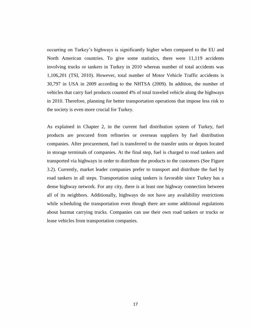
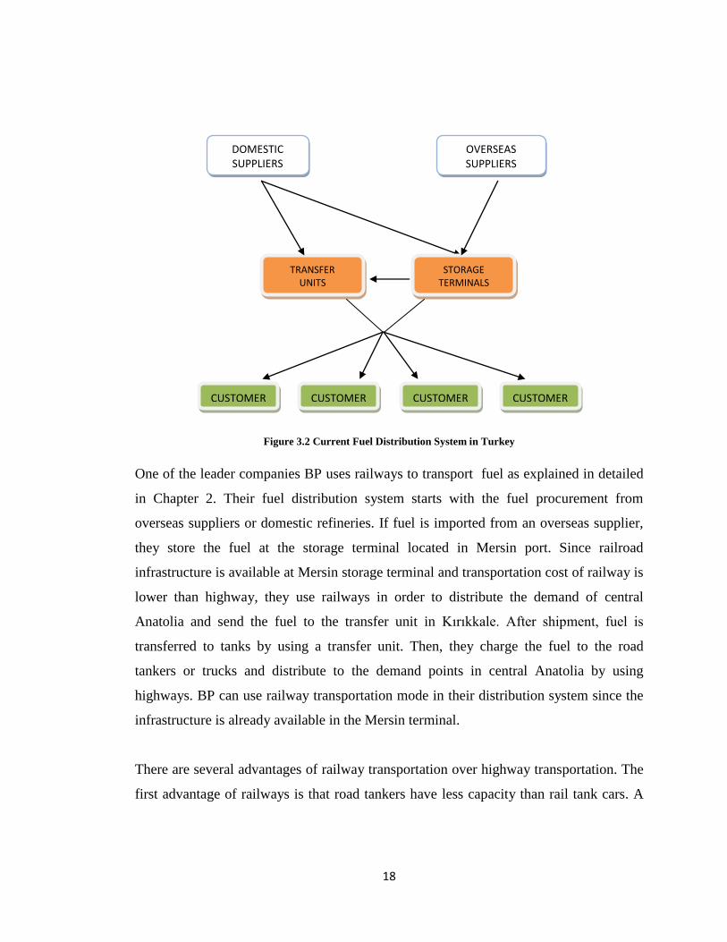
As explained in Chapter 2, in the current fuel distribution system of Turkey, fuel
products are procured from refineries or overseas suppliers by fuel distribution
companies. After procurement, fuel is transferred to the transfer units or depots located
in storage terminals of companies. At the final step, fuel is charged to road tankers and
transported via highways in order to distribute the products to the customers (See Figure
3.2). Currently, market leader companies prefer to transport and distribute the fuel by
road tankers in all steps. Transportation using tankers is favorable since Turkey has a
dense highway network. For any city, there is at least one highway connection between
all of its neighbors. Additionally, highways do not have any availability restrictions
while scheduling the transportation even though there are some additional regulations
about hazmat carrying trucks. Companies can use their own road tankers or trucks or
lease vehicles from transportation companies.
18
Figure 3.2 Current Fuel Distribution System in Turkey
One of the leader companies BP uses railways to transport fuel as explained in detailed
in Chapter 2. Their fuel distribution system starts with the fuel procurement from
overseas suppliers or domestic refineries. If fuel is imported from an overseas supplier,
they store the fuel at the storage terminal located in Mersin port. Since railroad
infrastructure is available at Mersin storage terminal and transportation cost of railway is
lower than highway, they use railways in order to distribute the demand of central
Anatolia and send the fuel to the transfer unit in Kırıkkale. After shipment, fuel is
transferred to tanks by using a transfer unit. Then, they charge the fuel to the road
tankers or trucks and distribute to the demand points in central Anatolia by using
highways. BP can use railway transportation mode in their distribution system since the
infrastructure is already available in the Mersin terminal.
There are several advantages of railway transportation over highway transportation. The
first advantage of railways is that road tankers have less capacity than rail tank cars. A
OVERSEAS SUPPLIERS
DOMESTIC SUPPLIERS
STORAGE TERMINALS
CUSTOMER CUSTOMER CUSTOMER CUSTOMER
TRANSFER UNITS
19
tanker can carry at most 27 tons of fuel between an origin and destination point. On the
other hand, railway tank wagons have approximately 55-60 tons of capacity. Another
advantage of railway transportation is that more than one wagon can move at the same
time. Furthermore, Turkish railroads mostly pass through rural areas. Thus, population
around the network is less when compared to the highway network. So, if an accident
occurs, the number of people exposed to danger will probability be lower than that of
highways. Consequently, we expect that including railway transportation into the current
distribution system will make the system preferable from both cost and risk perspectives.
The railroad alternative for fuel distribution and risk comparison of railroad and
highway options are not extensively studied for Turkey’s transportation infrastructure.
On the other hand, using only railways to distribute the fuel is not feasible since the
railway infrastructure is not available in all cities of Turkey. Therefore, a combination of
railway and highway transportation alternatives should be considered together. We refer
to such a combination as “intermodal transportation” from now on.
“Transportation of a person or a load from its origin to its destination by a sequence of at
least two transportation modes, the transfer from one mode to the next being performed
at an intermodal terminal” is one of the definitions of intermodal transportation in the
literature (Crainic and Kim, 2007). This definition applies to our approach in this study.
However, there are also some other definitions of intermodal transportation in the
literature such as “The carriage of goods by at least two different modes of transport in
the same loading unit (an Intermodal Transport Unit or ITU) without stuffing or
stripping operations when changing modes” (Arnold et al., 2004). In this study, the
transported goods are fuel products and they need to be shipped in the special fuel tanks
while using both transportation modes. Therefore, a unique transport unit cannot be
defined due to complexity of the nature of the fuel transportation nature.
20
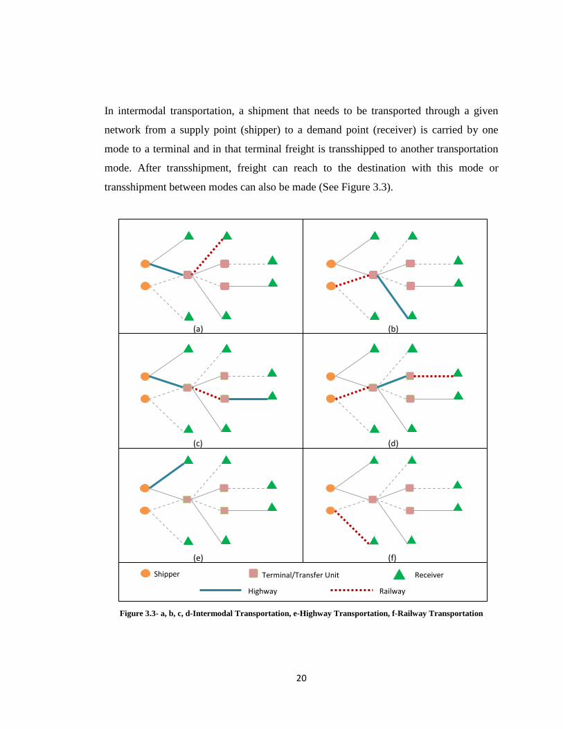
In intermodal transportation, a shipment that needs to be transported through a given
network from a supply point (shipper) to a demand point (receiver) is carried by one
mode to a terminal and in that terminal freight is transshipped to another transportation
mode. After transshipment, freight can reach to the destination with this mode or
transshipment between modes can also be made (See Figure 3.3).
Figure 3.3- a, b, c, d-Intermodal Transportation, e-Highway Transportation, f-Railway Transportation
Terminal/Transfer Unit Shipper Receiver
Highway Railway
(b) (a)
(d) (c)
(f) (e)
21
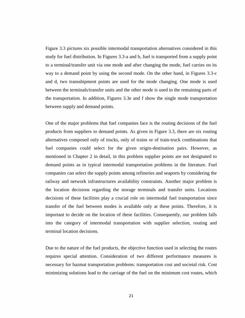
Figure 3.3 pictures six possible intermodal transportation alternatives considered in this
study for fuel distribution. In Figures 3.3-a and b, fuel is transported from a supply point
to a terminal/transfer unit via one mode and after changing the mode, fuel carries on its
way to a demand point by using the second mode. On the other hand, in Figures 3.3-c
and d, two transshipment points are used for the mode changing. One mode is used
between the terminals/transfer units and the other mode is used in the remaining parts of
the transportation. In addition, Figures 3.3e and f show the single mode transportation
between supply and demand points.
One of the major problems that fuel companies face is the routing decisions of the fuel
products from suppliers to demand points. As given in Figure 3.3, there are six routing
alternatives composed only of trucks, only of trains or of train-truck combinations that
fuel companies could select for the given origin-destination pairs. However, as
mentioned in Chapter 2 in detail, in this problem supplier points are not designated to
demand points as in typical intermodal transportation problems in the literature. Fuel
companies can select the supply points among refineries and seaports by considering the
railway and network infrastructures availability constraints. Another major problem is
the location decisions regarding the storage terminals and transfer units. Locations
decisions of these facilities play a crucial role on intermodal fuel transportation since
transfer of the fuel between modes is available only at these points. Therefore, it is
important to decide on the location of these facilities. Consequently, our problem falls
into the category of intermodal transportation with supplier selection, routing and
terminal location decisions.
Due to the nature of the fuel products, the objective function used in selecting the routes
requires special attention. Consideration of two different performance measures is
necessary for hazmat transportation problems: transportation cost and societal risk. Cost
minimizing solutions lead to the carriage of the fuel on the minimum cost routes, which
22
are composed of the shortest paths. These shortest paths mostly pass through the
population dense areas, therefore these paths may impose high risk to the public and
environment nearby. On the other hand, risk minimizing solutions carry the fuel mostly
through less populated and less congested areas by using possibly longer and circuitous
paths. Thus, these solutions may have high transportation costs compared to the cost
minimizing solutions. Consequently, a cost minimizing solution may not be the best
solution for the risk minimization objective and vice versa. Therefore, this problem has
multiple and conflicting objectives and priority of these performance measures may
differ depending on who the decision maker is. For instance, fuel companies may prefer
the cost minimizing solutions whereas public authorities may prefer risk minimizing (or
at least risk conscious) solutions. Even though cost minimization might be a priority
from the perspective of the fuel companies, extra regulations might be imposed on their
operations by the governmental institutions so that risk factor is also considered in
selecting transportation routes.
To sum up, the problem that we consider in this thesis is named as “Intermodal
Transportation of Hazardous Materials with Supplier Selection”. In particular, the aim is
to find routes between supply points and demand points on a given network composed
of highways and railways; and locate transshipment points on that network, so that
selected risk and/or cost measures are optimized in an appropriate manner.
23
Chapter 4
Literature Review
In this chapter, we analyze the intermodal transportation of hazardous materials
(hazmat) literature. For this purpose, we examine three different areas of the literature:
(1) Hazardous Materials Transportation, (2) Intermodal Transportation, and (3)
Intermodal Transportation of Hazardous Materials.
4.1. Hazardous Materials Transportation
Hazardous materials transportation problem has become significantly important for
decades due to the consequences of possible incidents/accident of transportation. Thus,
the aspects of the hazardous materials transportation attract an increasing attention from
researchers in years.
24
Hazmat incidents are considered as low-probability-high-consequence events. In these
types of events, the probability of the occurrence is low, whereas the impacts of
consequences are substantial. Due to the danger of hazardous materials, there are some
acts to minimize its threat that is exposed by public and environment like Uniform
Safety Act (1990) and The Canadian Environmental Protection Act (1988). In the
Canadian Act, the purpose is to design and enforce the suitable conditions to control
toxic materials transportation. There are some factors that affect the public sensitivity
such as inequity in the distribution of risks or the impact created by media (Erkut and
Verter, 1995).
In this part, we analyze the risk assessment and location/routing aspects of hazardous
materials literature, as they are closely related to our study. For other aspects, we refer
the reader to Erkut and Verter (1995).
Risk is the major component that separates hazmat transportation problems from other
transportation problems in the literature. Risk is defined as the measure of the
probability and severity of harm (Alp, 1995). Risk can be measured by qualitative or
quantitative methods. In the qualitative risk assessment, possible accident scenarios are
identified to estimate the undesirable consequences. This method is preferred if there is
lack of reliable data.
Quantitative methods on the other hand, involve three key steps; (1) hazard and exposed
receptor identification, (2) frequency analysis and (3) consequence modeling and risk
calculation. While evaluating the risk on the routes by following these steps, one of the
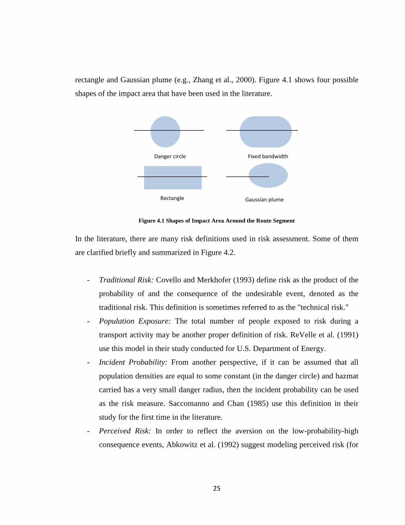
crucial decision is to decide on the shape of the impact area. There are different
geometric shapes that are used by researchers to model the impact area such as danger
circle (e.g., Erkut and Verter, 1998), fixed-bandwidth (e.g., ReVelle et al., 1991),
25
rectangle and Gaussian plume (e.g., Zhang et al., 2000). Figure 4.1 shows four possible
shapes of the impact area that have been used in the literature.
Figure 4.1 Shapes of Impact Area Around the Route Segment
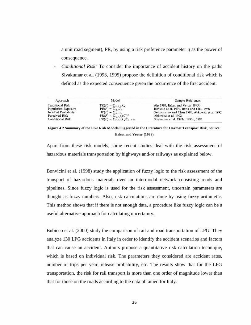
In the literature, there are many risk definitions used in risk assessment. Some of them
are clarified briefly and summarized in Figure 4.2.
- Traditional Risk: Covello and Merkhofer (1993) define risk as the product of the
probability of and the consequence of the undesirable event, denoted as the
traditional risk. This definition is sometimes referred to as the "technical risk."
- Population Exposure: The total number of people exposed to risk during a
transport activity may be another proper definition of risk. ReVelle et al. (1991)
use this model in their study conducted for U.S. Department of Energy.
- Incident Probability: From another perspective, if it can be assumed that all
population densities are equal to some constant (in the danger circle) and hazmat
carried has a very small danger radius, then the incident probability can be used
as the risk measure. Saccomanno and Chan (1985) use this definition in their
study for the first time in the literature.
- Perceived Risk: In order to reflect the aversion on the low-probability-high
consequence events, Abkowitz et al. (1992) suggest modeling perceived risk (for
Fixed bandwidth
Rectangle
Danger circle
Gaussian plume
26
a unit road segment), PR, by using a risk preference parameter q as the power of
consequence.
- Conditional Risk: To consider the importance of accident history on the paths
Sivakumar et al. (1993, 1995) propose the definition of conditional risk which is
defined as the expected consequence given the occurrence of the first accident.
Figure 4.2 Summary of the Five Risk Models Suggested in the Literature for Hazmat Transport Risk, Source:
Erkut and Verter (1998)
Apart from these risk models, some recent studies deal with the risk assessment of
hazardous materials transportation by highways and/or railways as explained below.
Bonvicini et al. (1998) study the application of fuzzy logic to the risk assessment of the
transport of hazardous materials over an intermodal network consisting roads and
pipelines. Since fuzzy logic is used for the risk assessment, uncertain parameters are
thought as fuzzy numbers. Also, risk calculations are done by using fuzzy arithmetic.
This method shows that if there is not enough data, a procedure like fuzzy logic can be a
useful alternative approach for calculating uncertainty.
Bubicco et al. (2000) study the comparison of rail and road transportation of LPG. They
analyze 130 LPG accidents in Italy in order to identify the accident scenarios and factors
that can cause an accident. Authors propose a quantitative risk calculation technique,
which is based on individual risk. The parameters they considered are accident rates,
number of trips per year, release probability, etc. The results show that for the LPG
transportation, the risk for rail transport is more than one order of magnitude lower than
that for those on the roads according to the data obtained for Italy.
27
Milazzo et al. (2002) analyze the of hazmat transportation through Messina town in
Sicily. They use a program called TRAT2 and analyze a case study of hazardous
materials transportation with different modes. The program has two main steps: (1)
analyzing the transport types in order to calculate the effects and vulnerabilities and (2)
data input including transport network, population distribution and factories location and
calculating the societal and individual risks. According to the output of the program,
they offer two different solutions to improve the safety of the territorial area.
Brown and Dunn (2007) present a study on the quantitative risk assessment for
evaluating consequence distributions of hazardous materials transportation. Their
method has a strong emphasis on consequence modeling and employs considerable
statistical data from past incidents. Initially they analyze the key statistical data which
includes geographical and temporal incident distributions, discharge fraction
distributions and meteorological database. Then they apply two classes of physical
models for incident modeling. First one is source emission modeling and second one is
atmospheric dispersion modeling. This technique provides analysis of thousands of
accident scenarios and application of consequence models in order to estimate the
percentage of time a certain protective action distance will be sufficient.
Another quantitative risk assessment study is conducted by Glickman et al. (2007). They
present a risk model, which quantifies the rail transport risk. They use the results of this
model with a weighted combination of cost to generate alternate routes. Seven factors
are used to assess the risk along each link of the network: (1) distances, (2) accident
rates, (3) total number of loaded cars per train, (4) number of tank cars per train loaded
with the hazardous material of concern, (5) conditional release probability, (6) the size
of the critical impact area and (7) population density in the critical impact area. As it is
explained further in details, this risk model is used as the basis of our risk assessment in
this thesis.
28
Next, we examine the location-routing category of the hazmat literature. In hazmat
transportation problem, there are multiple players such as carriers, shippers, insurers and
governments. Governments influence the carriers to prefer the routes with minimum risk
in order to minimize the consequences by applying some regulations over highways,
whereas carriers generally want to carry hazardous materials on the minimum cost
routes. Hence, hazmat transportation problem is a multi-objective problem with multiple
stakeholders. From this point of view, selection of the routes and locations of hazardous
facilities should satisfy both players in the system to the extent possible (Erkut et al.,
2007). Some of the recent studies related to location-routing problems in hazardous
materials literature are explained briefly below.
The first related study is conducted by Zografos and Samara (1989). Authors focus on
the hazardous wastes, which belong to class of miscellaneous dangerous goods of
hazmat categories (See Chapter 3). They consider the transportation of one type of
hazardous waste. They have multiple objectives, which are minimizing traveling time,
risk of transportation and risk of disposing the wastes. They propose a mixed-integer
goal-programming model and analyze the model on hypothetical data.
Later, List and Mirchandani (1991) examines a similar problem with multiple hazardous
waste/material types. The proposed model has multiple objectives, which are
minimization of risk, minimization of cost, and maximization of equity. Authors apply
their model on the real-life data obtained from capital district of Albany, NY.
Giannikos (1998) uses goal-programming technique top tackle with a similar problem.
The author develops a multi-objective location-routing model for hazardous waste
transportation. He determines four objectives, which are minimization of cost,
minimization of total perceived risk, the equitable distribution of risk among population
29
centers, and the equitable distribution of disutility caused by the operation of the
treatment facilities.
The most recent study on hazardous waste location routing problem is conducted by
Alumur and Kara (2007). Authors study the location and routing of the hazardous wastes
considering the compatibility issued among the different treatment technologies. They
develop a multi-objective mixed integer programming model, which decides the
locations of treatment and disposal centers, and routing of the hazardous wastes.
Objectives are minimizing the total cost and minimizing the transportation risk measured
by population exposure.
There are also some other location-routing studies which do not focus on only a single
class of hazardous materials. An example is by Halender and Melachrioudis (1997). The
authors study the integrated location routing problem in order to minimize the expected
number of hazardous material transportation accidents. They consider two different
routing policies, which are most reliable route planning and multiple routing with
random selection. According to these policies, the authors develop two location
models.In one of the recent studies, Cappanera et al (2004) use the Lagrangean
Relaxation method to separate the location-routing problem, which is NP-Hard, into two
sub-problems as location and routing problems.
4.2. Intermodal Transportation
Intermodal transportation is defined by Min (1991) as the movement of products from
origin to destination using a mixture of various transportation modes such as air, ocean
lines, barge, rail, and truck. Among these transportation modes, rail-truck combination is
the most common one researched in the literature.

30
In the rail-truck intermodal transportation (RTIM) the trucking part of the transport
chain is called drayage and the transported part by trains is called rail-haul. Another
important component of this system is the transshipment terminals where shipments
transferred from one mode to the other mode (See Figure 4.3).
Figure 4.3 Rail-Truck Intermodal Transportation, Source: Macharis and Bontekoning (2004)
There are some characteristics of rail-truck intermodal transportation, which are defined
by Bontekoning et al. (2004) (See Figure 4.4).
Figure 4.4 Rail-Truck Intermodal Transportation Characteristics, Source: Bontekoning et al (2004)
(a) Task division between modes with respect to the drayage and rail-haul parts of
the chain.
(b) Synchronized and seamless schedules between different modes.
(c) The use of standardized load units, which increases the efficiency in the transport
chain.
(d) Transshipment. The transshipment of load units is inherent to the division of tasks
between the short-haul and the long-haul. However, intermodal transshipment
distinguishes itself from other forms of transshipment for two reasons. First, it
involves transshipment from one mode to another; second, transshipment plays a
crucial role in a synchronized and often tight schedule.
(e) Multi-actor chain management. The level of complexity is higher in intermodal
transport chains with various organizations, each of them organizing and controlling
a part of the transport chain.
31
In the remaining part of this section, we analyzed the literature in four sub-categories:
studies that focus on (1) the whole intermodal network systems, (2) the drayage, (3) rail-
haul part, and (4) transshipment part of the intermodal transportation systems.
An example study of the general intermodal network systems is conducted by Chang
(2008). The author studies the problem of how to locate best routes for shipments
through the entire international intermodal network. He formulates this as a multi-
objective multimodal multi-commodity flow problem with time windows and concave
costs. The author also proposes a heuristic, which is based on relaxation and
decomposition techniques. First sub-problem is a bounded knapsack problem with upper
and lower bounds and the second sub-problem is solved by using Lagrangian sub-
gradient optimization method. A re-optimization method is used to deal with infeasible
solutions.
An application-motivated study is conducted by Caramia and Guerriero (2009). The
authors study a vehicle-routing problem, which aims to provide answers at the following
two planning levels: design of service network in order to define the best set of
transport services, and transportation programming in order to satisfy specific customer
requests. The purpose of the study is to minimize the traveling time and operating costs
together with the maximization of transportation mode sharing to improve capacity
utilization. They develop a heuristic algorithm composed of four steps: (1) computation
of all non-dominated paths, (2) removing the paths which are not viable, (3) minimizing
road service cost and (4) minimizing rail and maritime service time and costs. The
proposed algorithm is applied to a real-life case study in Italy.
The study by Moccia et al. (2010) is another application-oriented study which focuses
on the problem faced by a third party logistics company in Italy whose aim is to satisfy
customer demand through a minimum cost combination of rail and truck services with
32
different types of departure times. The considered problem is a multimodal
transportation problem with flexible time and scheduled service. The authors develop a
decomposition-based heuristic, which reflects the problem characteristics. They apply
the heuristic on the instances, which are generated from the case study of the logistic
company in Italy.
Drayage part of the rail-truck intermodal transportation is defined as the shipment
between shipper to terminal or terminal to receiver by using trucks. This part accounts
for a large percentage of origin to destination expenses. Major problems in drayage
operations are the planning and scheduling of trucks between the terminals and
shippers/receivers. These problems can be analyzed in three sub-categories: problems at
strategic level, tactical level and operational level.
The main problems at the strategic level deal with the transportation activities between
shippers and terminals or terminals and receivers. An example is given by Zhang et al.
(2011). The authors study the problem of transporting containers by trucks with the three
main movement types; incoming to terminal with loaded trucks, outgoing from terminal
with loaded trucks, and incoming to terminal with empty trucks. They consider the
resource constraints and time spent at the shippers’ and receivers’ terminals. They
formulate the problem as a directed graph in order to develop a mathematical model. A
search algorithm is used to solve the problem.
At the tactical level, most common problems are the assignment problems of shipper
locations to terminals or service areas and routing problems. An example study is
conducted by Taylor et al. (2002). The authors generate two alternative heuristics and
analyze 40 different scenarios for the terminal selection problem.
33
Lastly, for the operational level, Justice (1996) deals with the problem of planning when,
where and how many intermodal truck chassis are redistributed among the terminals.
The problem is mathematically formulated as a bi-directional time based (network)
transportation problem and applied to eight interconnected terminals in the USA.
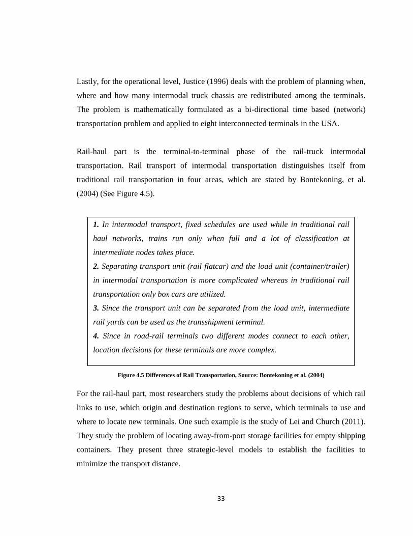
Rail-haul part is the terminal-to-terminal phase of the rail-truck intermodal
transportation. Rail transport of intermodal transportation distinguishes itself from
traditional rail transportation in four areas, which are stated by Bontekoning, et al.
(2004) (See Figure 4.5).
Figure 4.5 Differences of Rail Transportation, Source: Bontekoning et al. (2004)
For the rail-haul part, most researchers study the problems about decisions of which rail
links to use, which origin and destination regions to serve, which terminals to use and
where to locate new terminals. One such example is the study of Lei and Church (2011).
They study the problem of locating away-from-port storage facilities for empty shipping
containers. They present three strategic-level models to establish the facilities to
minimize the transport distance.
1. In intermodal transport, fixed schedules are used while in traditional rail
haul networks, trains run only when full and a lot of classification at
intermediate nodes takes place.
2. Separating transport unit (rail flatcar) and the load unit (container/trailer)
in intermodal transportation is more complicated whereas in traditional rail
transportation only box cars are utilized.
3. Since the transport unit can be separated from the load unit, intermediate
rail yards can be used as the transshipment terminal.
4. Since in road-rail terminals two different modes connect to each other,
location decisions for these terminals are more complex.
34
Transshipment part of the rail-truck transportation deals with the location, layout and
transshipment operations at the road–rail terminals and rail–rail terminals.
Arnold et al. (2004) propose a study about developing a model for locating rail/road
terminals optimally for freight transport. A 0-1 program is formulated and solved by a
heuristic approach, which is applied in Iberian Peninsula. The model used in this study is
similar to multi-commodity fixed charge network design problems. The authors consider
a terminal as an arc not as a vertex. This approach reduces the number of decision
variables. The heuristic procedure use shortest paths and consider three important
criterion; (1) total transportation cost, (2) total quantity passing through the transfer arcs
and (3) total flow.
Boysen and Pesch (2008) deal with the train scheduling problem at the transshipment
yard. They investigate the resolving deadlocks and avoiding multiple crane picks per
container move and develop a mathematical model with the exact and heuristic
procedures.
Caris and Janssens (2009) study the container hauling at the intermodal transshipment
terminal. They model the problem as a full truckload pickup and delivery problem with
time windows. The purpose is to find the assignments of delivery and pickup customer
pairs in order to minimize the total cost. They develop a two-phase heuristic where the
first phase finds the initial assignment combinations and the second phase improves by
the local search.
Boysen et al. (2010) focus on the problem of determining yard areas for gantry cranes in
order to spread the workload among the cranes. They develop a dynamic programming
35
approach to deal with this problem. The results of a simulation indicate that if optimal
crane areas are applied, train processing activities speed-up.
4.3. Intermodal Transportation of Hazardous Materials
Rail–truck intermodal transportation (RTIM) has a very important advantage that it
combines the accessibility of road networks and cost effectiveness of railroad shipments.
Additionally, rail-truck intermodal transportation attracts attention from shippers since
intermodal trains are reliable for on-time deliveries.
Since the transported volume of hazmat has increased over the years, the advantage of
rail-truck intermodal transportation became more important in order to minimize the cost
and the risk imposed on public. A substantial advantage of rail transportation is that
trains can carry non-hazardous and hazardous goods together whereas these two types
are almost never mixed in truck shipments. Additionally, a rail tank is three times the
capacity of a truck-tanker (Verma and Verter (2007).
Drayage, rail-haul, and transshipment parts are also valid for intermodal transportation
of hazardous materials. Drayage is the transportation part between shippers to terminals
or terminals to receivers. Rail-haul part is the terminal-to-terminal transportation and
transshipment is the transfer activity of hazmat between modes.
Although hazardous materials are transported with rail-truck intermodal systems,
particularly in Europe and Canada in past the decades, intermodal transportation od
hazmats received less attention from researchers in operational research literature
There are two recent studies that focus on the intermodal transportation of hazmats
(Verma (2009), Verma and Verter (2010)). Verma (2009) is the first application oriented
study that focuses on the tactical planning problem of a railroad company that regularly
36
transports a predetermined amount of hazardous and non-hazardous cargo across a
railroad network, from a set of origin yards to a set of destination yards. He develops a
bi-objective optimization model. The cost is determined based on the railroad
transportation industry and the risk is determined from the incorporation of the railroad
accident rates. The optimization model and the solution framework are used to solve a
realistic-size problem instance based in southeast USA.
Later, Verma and Verter (2010) focus on the general version of the intermodal
transportation of hazardous materials. The authors study the problem of planning the
rail-truck intermodal transportation. Their purpose is to determine the best shipment plan
for both hazardous and non-hazardous freight in a rail-truck intermodal network,
wherein a set of pre-specified lead times must be satisfied in choosing the truck routes
and the intermodal train services to be used. The objectives are; minimizing the total
cost of transportation and the total public risk associated with hazmats. They develop a
bi-objective optimization model to manage intermodal shipments. Lead-times, which are
specified by customers, are considered in intermodal route selection. They develop an
iterative decomposition based solution methodology. They decompose the original
problem into two sub-problems: rail-haul and drayage. Rail-haul part aims to find the
optimal rail travel time for each shipment. These rail travel times are taken into account
in drayage part of the problem as parameters of the lead-time constraints. They apply
the method on an instance, based on the intermodal service network in eastern USA.
Recall that the main purpose of our problem is to find routes between supply points and
demand points on a given network; and to locate the transshipment points on that
network so that selected risk and/or cost measures are optimized. The problem
considered by Verma and Verter (2010) is the most similar study to our problem since
their purpose is to find the optimal routing plan for hazardous materials transportation.
However, there are some aspects, which are different in our problem. In their study,
37
origin-destination pairs are given whereas in our case origins are not given. In fact, our
problem investigates which demand point is served from which supplier and to what
extent. Since supplier selection is an important decision of the problem, we believe that
this aspect makes our problem more realistic. Moreover, they consider the lead times
specified by customers, which are not considered in our study. Another difference is
that, unlike us they decompose the model into two sub problems: drayage and rail-haul,
and the locations of the transshipment terminals are given in their study whereas location
decisions of these points play a crucial part in our problem. They use only two
transshipment terminals and the intermodal connections are materialized only in these
terminals, which makes their study restrictive when compared to our model.
38
Chapter 5
Model Development
In this chapter, firstly, we introduce a transportation risk model for highway and railway
transportation. Secondly, we propose a mathematical model, which aims to find the
paths that connect supply and demand points so that all demand is satisfied, by deciding
on the transportation mode that will be used on the arcs along the paths and locating the
transshipment points in a safe and cost effective manner.
5.1. Transportation Risk Model
In this section, highway and railway risk models are explained in details.
39
5.1.1. Highway Risk Model
There are different transportation risk definitions in the hazardous materials
transportation literature as stated in Chapter 4 in details. Some definitions rely on an
expected risk measure, which considers probability of incidents and consequence of the
events simultaneously. Traditional risk and perceived risk definitions are in this
category. Some definitions consider only the probability of incidents on the route or
their consequence. Incident probability and conditional risk definitions belong to these
categories. Additionally, some other definitions, such as population exposure, consider
the number of effected people inside of the impact area (See Figure 4.1 of Chapter 4).
Among these different definitions, traditional risk definition is the one that is used as the
risk measure in this study.
In this model, risk of traversing a highway arc (i,j) is defined as;
where
Distances of arc (i,j) on the highway network
δh Accident rate over highways
pr Conditional probability of the release of hazardous material when an accident
occurs
Population density in the critical area of exposure along of highway arc (i,j)
The total risk of a path P between an origin and destination is estimated as the
summation of the risks of individual arcs along that path. This way of calculating the
risk of a path is not an exact method however, the resulting error rate is negligible. For a
40
detailed discussion of this issue, we refer the reader to Erkut and Verter (1995).
Consequently, if all (i,j) along P are highway connections, total risk of the path P is
calculated as
5.1.2. Railway Risk Model
Even though there are different risk definitions to measure the transportation risk of
highways, there are just a few studies that focus on railway transportation risk. Some
studies based the risk measure on the population exposure (Verma and Verter, 2007) or
on the individual risk calculation (Bubicco et al. (2000), Milazzo et al. (2002)) and some
of them focused on the quantitative assessment of expected consequence (Glickman et
al. (2007), Brown and Dunn (2007)). Details of these studies can be found in Chapter 4.
In this study, we basically adapt the risk model of Glickman et al. (2007) and modify the
original model slightly to better represent our case. Summary of the notations used in the
model is given in the Table 5.1.
Table 5-1 Notations Used in Railway Risk Model
Notations
Distance of arc (i,j) on railway network in kilometers
δr Accident rate over railways
pr
Conditional probability of the release of hazardous material when an accident
occurs
pd Derailment probability
The population density of arc (i,j) in the critical impact area
X The number of tank cars per train loaded with the hazardous material of
concern
XD The number of tank cars loaded with hazmat that are damaged or derailed
XR The number of tank cars that experience a major release
41
Similar to the highway risk definition, risk of traversing a railway arc (i,j) is defined as,
where
fij Expected percentage of trains on link (i,j) that experience an accident involving a
major release of the hazardous material of concern
Nij Expected consequence of such an accident measured by the expected number of
residents in the critical area of exposure along arc (i, j).
The total risk of a path P between an origin and destination, if all (i,j) along P are
railway connections, is also calculated similar to that of the highway risk model as
A locomotive can pull railcars loaded with hazardous and non-hazardous materials
simultaneously. Amount of fuel that needs to be transported every day is substantial
quantity due to very high demand. If railways are used as an alternative transportation
mode for fuel distribution, this high demand would result with the requirement of too
many railcars and hence trains used for this purpose would pull railcars that are loaded
only with fuel.
A railway accident could be a derailment, a head-on collision or a rear collision with a
train. In most of these accidents, only a part of the tank cars damage or derail.
Sometimes these cars located in the head/end part of train and sometimes located in the
middle of the train. Additionally, it is not always the case that all damaged/derailed cars
experience a release. In some accidents, even if there are derailed/damaged tank cars,
there are might be no release of the hazmat.
42
Having these in mind, we need to estimate the number of wagons that carry fuel
products (X), the number of wagons that are derailed/damaged (XD) and number of
wagons that experience a release (XR) in order to calculate fij, which is defined as the
expected percentage of trains on link (i, j) that experience an accident involving a major
release of the hazardous material of concern. The formula is
where
δr Accident rate over railways
Distance of arc (i,j) on the railway network
P(XR > 0) Probability of experiencing a major release.
Here, XR, which is defined as the number of wagons that experience a major release,
depends on the number of loaded tank cars that are damaged or derailed (XD). We can
estimate the probability of a release for a given number of tank cars that are
derailed/damaged as a conditional probability, denoted by P(XR|XD). Glickman et al.
(2007) assumed that this probability is binomially distributed. This probability
distribution assumes that occurrence of a tank car releases is a Bernoulli process, where
each of the damaged or derailed tank cars (XD) has a release probability p. Consequently,
probability distribution P(XR) can be estimated as,
where P(XD) is defined as the probability of derailment which is dependent on the total
number of loaded tank cars (X). In this study, we model P(XD) with negative binomial
distribution, as the details are explained in Chapter-6.
43
The other component of Rrij that we need to estimate is Nij, which is the expected
consequence of an hazmat incident occurred along arc (i, j). Nij can be estimated by,
where is the population density along the railway arc of exposure and the second
component is the expected tank cars that experience a release.
To sum up, after calculating the fij and Nij values, the risk associated with traversing arc
(i,j) is computed by the product of these values.
5.2. Mathematical Model
In this section, we propose a mathematical model which aims to find an intermodal
network composed of highway and railway infrastructure through which fuel products
are carried from sources to destinations in a safe and cost effective manner and to
determine the optimal locations of transfer units and depots that makes this distribution
possible.
In this study, the highway and railway networks are incomplete networks in which every
pair of distinct nodes is not connected with a unique edge. Therefore, we define two new
parameters correspond to the availabilities in which the existent edges on the current
infrastructure are considered as the available edges for both highway and railway
networks. However, we set all of the edges of railway network as available due to the
fact that estimated distances are composed of shortest paths for each pair of distinct
nodes on the railway network.
44
The proposed mathematical model for fuel transportation can be stated as follows: Given
the railway and highway transportation network and the set of potential nodes for
transfer units and depots, find the location of transfer units and the amount of
transported fuel products between origin and destination points and find the supplied
amounts from suppliers in the given transportation network so as to minimize the
transportation risk and/or cost.
The following indices and parameters are used in the mathematical formulation.
Given;
N={1,…,n} Cities
Parameters:
ch cost of transporting one unit of fuel oil by highway
cr cost of transporting one unit of fuel oil by railway
aij 1 if link (i, j) is an available highway arc, 0 otherwise
bij 1 if link (i, j) is an available railway arc, 0 otherwise
distance of link (i,j) on highway
distance of link (i,j) on railway
wi demand of city i
oi 1 if city i is a supply point, 0 otherwise
di 1 if city i has a depot, 0 otherwise
kD capacity of depots
kTU
capacity of transfer units
pTU
number of transfer units to be opened
transportation risk of highway link (i,j)
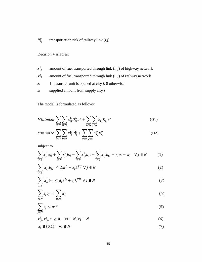
45
transportation risk of railway link (i,j)
Decision Variables:
amount of fuel transported through link (i, j) of highway network
amount of fuel transported through link (i, j) of railway network
zi 1 if transfer unit is opened at city i, 0 otherwise
si supplied amount from supply city i
The model is formulated as follows:
subject to
46
Objective O1 is the cost objective minimizing the total cost of transporting fuel products
through highways and railways. The amount of transported fuel products on a given link
multiplied with distance of that link times unit transportation cost is to be minimized.
Objective O2 is the risk objective minimizing the total transportation risk. The assigned
risk value of a given link times the amount of transported fuel products on that link is to
be minimized. As the risk values of links are different between highways and railways
the equation is summed for both modes.
Constraint set (1) is the flow balance constraints for the transportation of fuel products.
This constraint set ensures that the demanded amount of fuel is satisfied for all cities by
considering the mode availabilities. Also, this constraint set assures that the amount of
fuel generated at supply points must be transported from these points to cities.
Constraint sets (2) and (3) correspond to availability constraints for railway
transportation by considering the locations of depots and transfer units. This constraint
ensures that railway could only be used on a given link if there is a depot or transfer unit
located at the origin or destination of that link. Also this constraint guarantees that the
shipped amount of fuel to points which has a depot or a transfer unit cannot exceed the
capacity of a depot or a transfer unit.
Constraint set (4) is the supplier selection constraint for demand points. By this
constraint, model chooses how much of demand is supplied from the available supply
points.
Constraint set (5) correspond to the location constraint for transfer units. The constraints
assure that the number of opened transfer unit cannot exceed the designated amount.
47
The other constraint sets that are left are the non-negativity constraints and the
constraints defining the binary variables. The model has 11,935 continuous variables
(xh
ij, xrij, si), 77 binary variables (zi) and 12,245 constraints for a typical problem
generated for Turkey.
Observe here that, if the decision maker prefers to allow opening new depots, parameter
di can be considered as a decision variable.
Next, we create four versions of this base model depending on the prior objective
selected. The first two models consider only one of the objectives:
MC:
subject to
MR:
subject to
Third model assumes the risk objective function but an upper bound on the total cost of
transportation is imposed in the constraints and last model assumes the cost objective
function but an upper bound on the total risk of transportation is imposed in the
constraints
48
MR-βCost:
subject to
MC-γRisk:
subject to
Fuel companies (or the carrier companies that they delegate their transportation
operations) are the decision makers of the problem under concern. Since these
companies are profit seeking private companies, their first priority would be "cost
minimization" and hence MC would be their choice among the above models. If the
decision maker were the "public" whose concern is just to minimize the "risk" of
transportation then the decision maker's choice would definitely be the MR model. Due
to the infrastructure of transportation networks, MR and MC models produce conflicting
solutions, meaning that the minimum cost solution yields high risky transportation
whereas minimum risk solution yields high cost transportation. Therefore, governments
(with an aim of reflecting the public view) try to motivate or force the decision makers
to deviate from their MC solution towards less risky paths, by imposing regulations and
legislations. If the government asks carrier companies’ to choose paths of which risk
value is no more than a predefined level then the decision maker solves the MC-Risk
model. On the other hand, if the government motivates the decision maker to operate
with a cost figure that is higher than their minimum cost with an acceptable margin (for
49
example, carrier agrees to operate with a total transportation cost 10% higher than the
minimum cost possible) then MR-Cost would be the right choice for the decision
maker.
Furthermore, we know that railway transportation is cost wise advantageous when
compared to highway transportation. Hence, we use MR-βCost model in our numerical
analyses in order to observe maximum benefit that can be achieved on the total
transportation risk. For preliminary runs, we use both MR-βCost and MC-γRisk models
and results indicate that the numerical insights are not very different from each other.
50
Chapter 6
Data Collection and Computational
Results
In this section, our aim is to show the potential benefits of using railways in conjunction
with highways in Turkey's fuel distribution system, from both risk and cost perspectives.
In order to make our analysis as realistic as possible, we collected all kinds of relevant
and realistic data as much as possible. In Section 6.1, we summarize the data collected.
In Section 6.2, we present our numerical analysis.
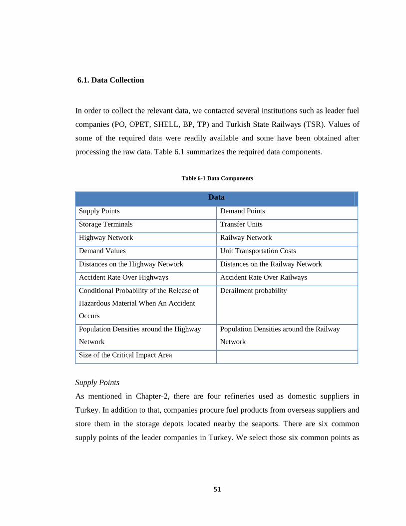
51
6.1. Data Collection
In order to collect the relevant data, we contacted several institutions such as leader fuel
companies (PO, OPET, SHELL, BP, TP) and Turkish State Railways (TSR). Values of
some of the required data were readily available and some have been obtained after
processing the raw data. Table 6.1 summarizes the required data components.
Table 6-1 Data Components
Data
Supply Points Demand Points
Storage Terminals Transfer Units
Highway Network Railway Network
Demand Values Unit Transportation Costs
Distances on the Highway Network Distances on the Railway Network
Accident Rate Over Highways Accident Rate Over Railways
Conditional Probability of the Release of
Hazardous Material When An Accident
Occurs
Derailment probability
Population Densities around the Highway
Network
Population Densities around the Railway
Network
Size of the Critical Impact Area
Supply Points
As mentioned in Chapter-2, there are four refineries used as domestic suppliers in
Turkey. In addition to that, companies procure fuel products from overseas suppliers and
store them in the storage depots located nearby the seaports. There are six common
supply points of the leader companies in Turkey. We select those six common points as
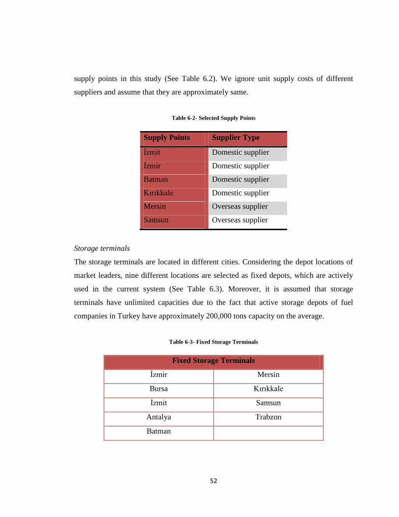
52
supply points in this study (See Table 6.2). We ignore unit supply costs of different
suppliers and assume that they are approximately same.
Table 6-2- Selected Supply Points
Supply Points Supplier Type
Ġzmit Domestic supplier
Ġzmir Domestic supplier
Batman Domestic supplier
Kırıkkale Domestic supplier
Mersin Overseas supplier
Samsun Overseas supplier
Storage terminals
The storage terminals are located in different cities. Considering the depot locations of
market leaders, nine different locations are selected as fixed depots, which are actively
used in the current system (See Table 6.3). Moreover, it is assumed that storage
terminals have unlimited capacities due to the fact that active storage depots of fuel
companies in Turkey have approximately 200,000 tons capacity on the average.
Table 6-3- Fixed Storage Terminals
Fixed Storage Terminals
Ġzmir Mersin
Bursa Kırıkkale
Ġzmit Samsun
Antalya Trabzon
Batman
53
Transfer Units
BP is the only company that uses railroads for distributing fuel products; hence, only BP
operates transfer units. In rail transportation, after the fuel is charged into rail tank
wagons in storage terminals or in refineries, fuel is transported to the transfer stations.
At these stations, fuel is transferred from tank wagons to road tankers by using a storage
tank or the transfer unit. In the current system, two transfer units are operating actively
(See Table 6.4), therefore these locations are selected as fixed points. Further, opening
new transfer units will be analyzed by considering the potential locations. Furthermore,
capacity of a transfer unit is estimated based on the maximum discharging time of a fuel
tanker whose capacity is 27 tons. It is assumed that transfer units could operate 24 hours
a day and 30 days in month. Hence, after calculations, the estimated capacity is set to
97,200 tons/month for one transfer unit.
Table 6-4- Selected Transfer Units
Active Transfer Units
Kırıkkale
Ankara
Demand Points and Values
We have condensed the total demand of all demand sources in a city into a single
demand point, which is denoted by the center of the city. Consequently, locations of the
final customers in our models correspond to the city centers. Tactical and operational
decisions of fuel distribution inside a city are kept out of the scope of this study. In the
current infrastructure, railway transportation from Anatolian region to Thrace region is
not available and there is only one highway passage from Anatolia to Thrace. Therefore,
cities in Thrace region and the city of Istanbul are omitted from demand points set.
Consequently, 77 cities are determined as demand points. Demands of the cities are
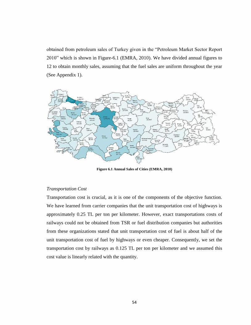
54
obtained from petroleum sales of Turkey given in the “Petroleum Market Sector Report
2010” which is shown in Figure-6.1 (EMRA, 2010). We have divided annual figures to
12 to obtain monthly sales, assuming that the fuel sales are uniform throughout the year
(See Appendix 1).
Figure 6.1 Annual Sales of Cities (EMRA, 2010)
Transportation Cost
Transportation cost is crucial, as it is one of the components of the objective function.
We have learned from carrier companies that the unit transportation cost of highways is
approximately 0.25 TL per ton per kilometer. However, exact transportations costs of
railways could not be obtained from TSR or fuel distribution companies but authorities
from these organizations stated that unit transportation cost of fuel is about half of the
unit transportation cost of fuel by highways or even cheaper. Consequently, we set the
transportation cost by railways as 0.125 TL per ton per kilometer and we assumed this
cost value is linearly related with the quantity.
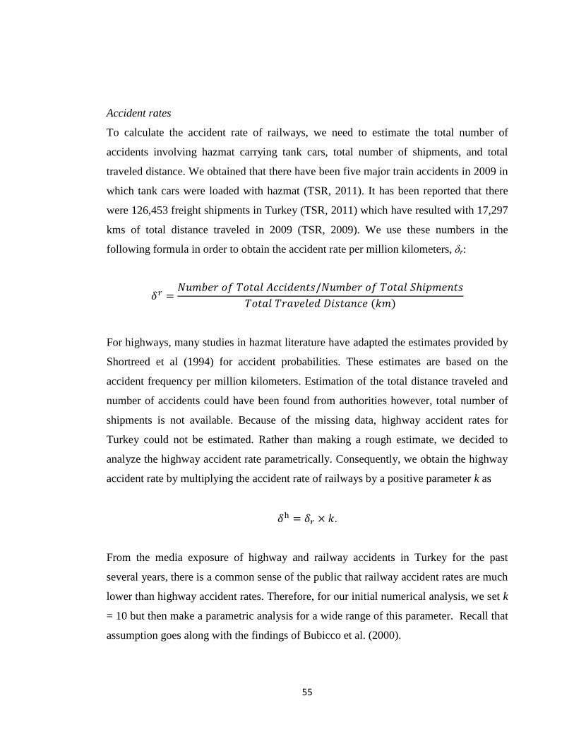
55
Accident rates
To calculate the accident rate of railways, we need to estimate the total number of
accidents involving hazmat carrying tank cars, total number of shipments, and total
traveled distance. We obtained that there have been five major train accidents in 2009 in
which tank cars were loaded with hazmat (TSR, 2011). It has been reported that there
were 126,453 freight shipments in Turkey (TSR, 2011) which have resulted with 17,297
kms of total distance traveled in 2009 (TSR, 2009). We use these numbers in the
following formula in order to obtain the accident rate per million kilometers, δr:
For highways, many studies in hazmat literature have adapted the estimates provided by
Shortreed et al (1994) for accident probabilities. These estimates are based on the
accident frequency per million kilometers. Estimation of the total distance traveled and
number of accidents could have been found from authorities however, total number of
shipments is not available. Because of the missing data, highway accident rates for
Turkey could not be estimated. Rather than making a rough estimate, we decided to
analyze the highway accident rate parametrically. Consequently, we obtain the highway
accident rate by multiplying the accident rate of railways by a positive parameter k as
.
From the media exposure of highway and railway accidents in Turkey for the past
several years, there is a common sense of the public that railway accident rates are much
lower than highway accident rates. Therefore, for our initial numerical analysis, we set k
= 10 but then make a parametric analysis for a wide range of this parameter. Recall that
assumption goes along with the findings of Bubicco et al. (2000).
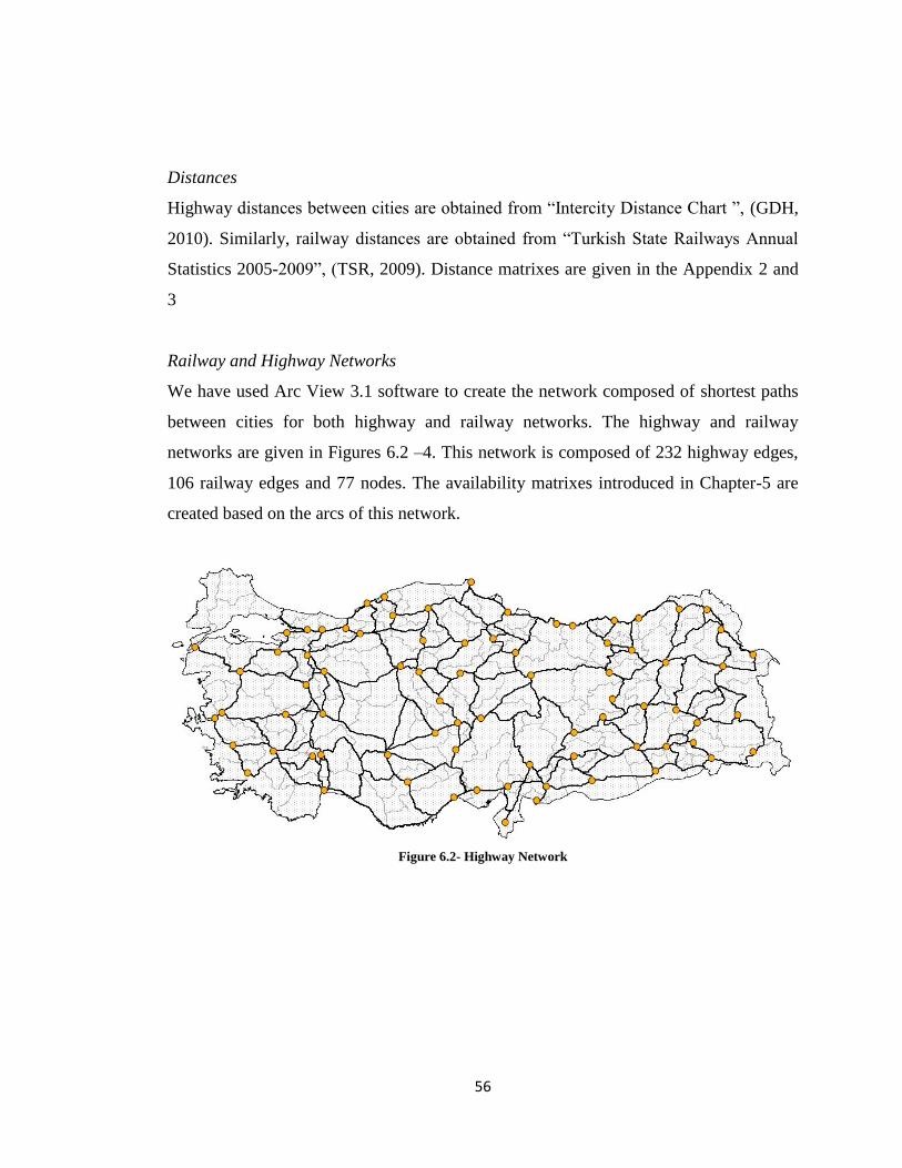
56
Distances
Highway distances between cities are obtained from “Intercity Distance Chart ”, (GDH,
2010). Similarly, railway distances are obtained from “Turkish State Railways Annual
Statistics 2005-2009”, (TSR, 2009). Distance matrixes are given in the Appendix 2 and
3
Railway and Highway Networks
We have used Arc View 3.1 software to create the network composed of shortest paths
between cities for both highway and railway networks. The highway and railway
networks are given in Figures 6.2 –4. This network is composed of 232 highway edges,
106 railway edges and 77 nodes. The availability matrixes introduced in Chapter-5 are
created based on the arcs of this network.
Figure 6.2- Highway Network
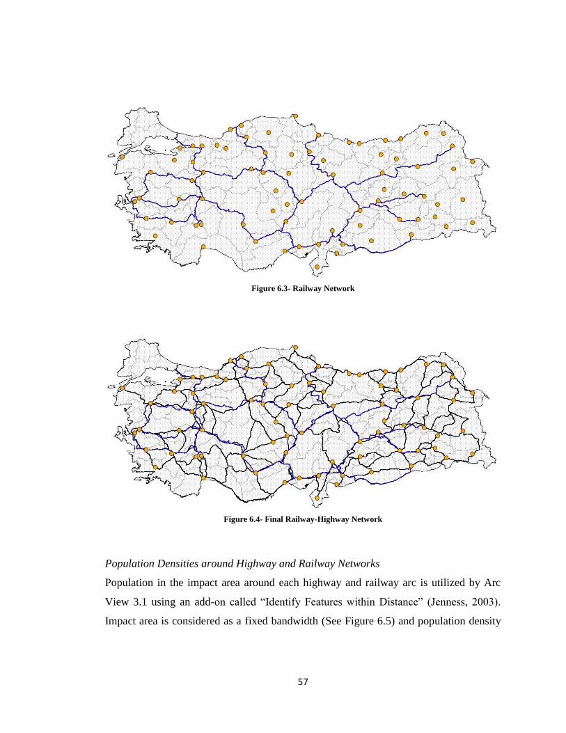
57
Figure 6.3- Railway Network
Figure 6.4- Final Railway-Highway Network
Population Densities around Highway and Railway Networks
Population in the impact area around each highway and railway arc is utilized by Arc
View 3.1 using an add-on called “Identify Features within Distance” (Jenness, 2003).
Impact area is considered as a fixed bandwidth (See Figure 6.5) and population density
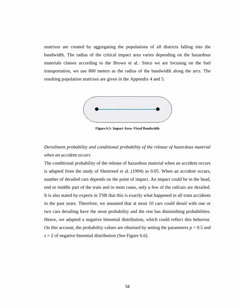
58
matrixes are created by aggregating the populations of all districts falling into the
bandwidth. The radius of the critical impact area varies depending on the hazardous
materials classes according to the Brown et al.. Since we are focusing on the fuel
transportation, we use 800 meters as the radius of the bandwidth along the arcs. The
resulting population matrixes are given in the Appendix 4 and 5.
Figure 6.5- Impact Area- Fixed Bandwidth
Derailment probability and conditional probability of the release of hazardous material
when an accident occurs
The conditional probability of the release of hazardous material when an accident occurs
is adapted from the study of Shortreed et al. (1994) as 0.05. When an accident occurs,
number of derailed cars depends on the point of impact. An impact could be in the head,
end or middle part of the train and in most cases, only a few of the railcars are derailed.
It is also stated by experts in TSR that this is exactly what happened in all train accidents
in the past years. Therefore, we assumed that at most 10 cars could derail with one or
two cars derailing have the most probability and the rest has diminishing probabilities.
Hence, we adapted a negative binomial distribution, which could reflect this behavior.
On this account, the probability values are obtained by setting the parameters p = 0.5 and
s = 2 of negative binomial distribution (See Figure 6.6).
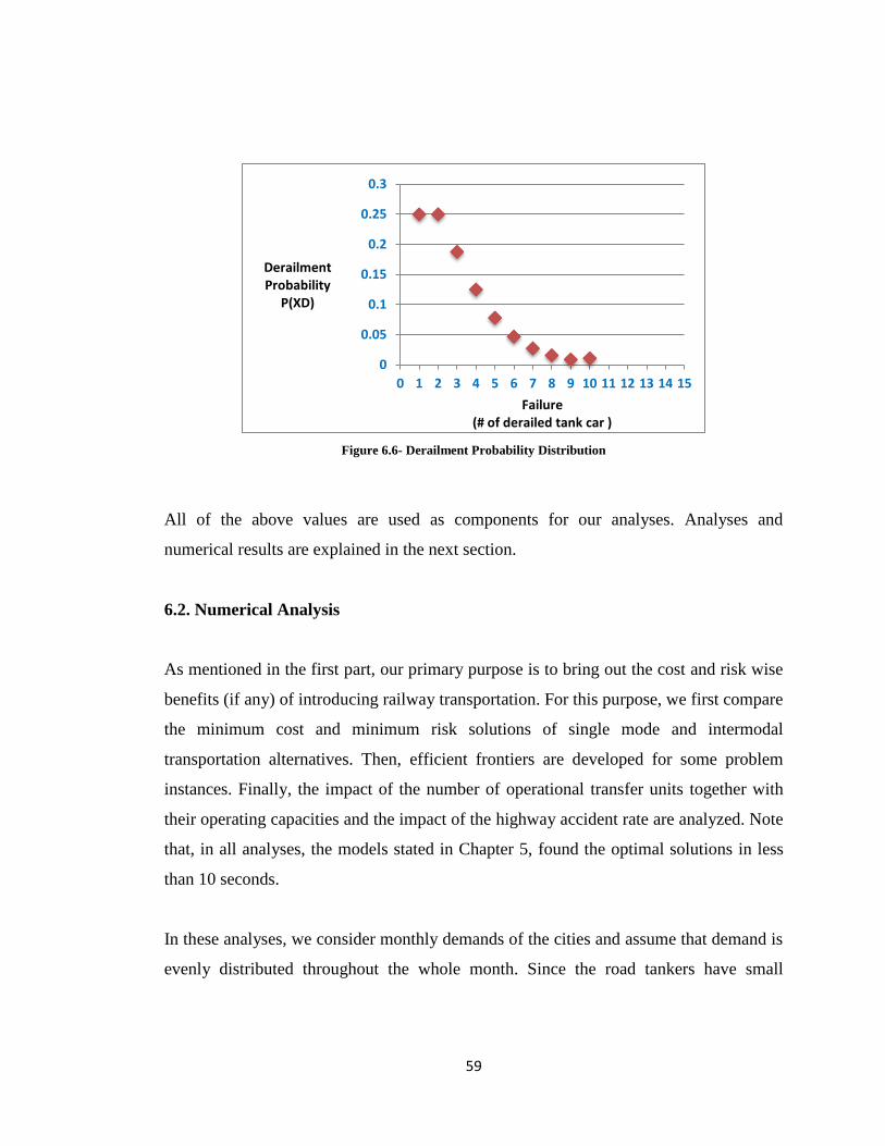
59
Figure 6.6- Derailment Probability Distribution
All of the above values are used as components for our analyses. Analyses and
numerical results are explained in the next section.
6.2. Numerical Analysis
As mentioned in the first part, our primary purpose is to bring out the cost and risk wise
benefits (if any) of introducing railway transportation. For this purpose, we first compare
the minimum cost and minimum risk solutions of single mode and intermodal
transportation alternatives. Then, efficient frontiers are developed for some problem
instances. Finally, the impact of the number of operational transfer units together with
their operating capacities and the impact of the highway accident rate are analyzed. Note
that, in all analyses, the models stated in Chapter 5, found the optimal solutions in less
than 10 seconds.
In these analyses, we consider monthly demands of the cities and assume that demand is
evenly distributed throughout the whole month. Since the road tankers have small
0
0.05
0.1
0.15
0.2
0.25
0.3
0 1 2 3 4 5 6 7 8 9 10 11 12 13 14 15
Derailment Probability
P(XD)
Failure (# of derailed tank car )
60
capacities, monthly demand of a city is to be shipped in several trips throughout the
month. For the cities in which railway infrastructure is available, the city of Mus has the
minimum demand: 1,461 tones. A railway tank wagon accommodates approximately 60
tones of fuel, therefore the total demand of Mus can be shipped with at least 24 wagons.
In our numerical studies we set X, the number of tank cars per train loaded with the
hazardous material of concern, to a value of 10. So the demand of Mus, if transported
with railways, is to be shipped in three trips. We assume that these three trips are evenly
distributed in the whole month. Similarly, the city of Ankara has the maximum demand:
103,353.5 tones and if this demand is transported with railways, it is to be shipped in
approximately 170 trips which are evenly distributed in the whole month.
Finally, we note that we conducted our numerical analysis by aggregating the demands
and operations of the four major fuel distribution companies, assuming that they obey to
a central authority. In practice, apparently this is not the case but our aim in our
numerical analysis is show the maximum benefit of intermodal transportation in case all
companies adapt intermodal transportation for their operations. Hence, some of the
insights that we generate in our numerical analysis might not hold if only a subset of the
companies adapt intermodal transportation.
6.2.1. Analysis of Single Mode vs. Intermodal Transportation
The main purpose in this sub-section is to observe the estimated benefits of the
transportation with railways from cost and risk perspectives. To this end, we compared
the Min Cost (Model MC) and Min Risk (Model MR) solutions of preferring single
mode or intermodal transportation.
Current fuel distribution system in Turkey is mainly composed of highways. Carriers
prefer using highway alternative for distributing the fuel between suppliers and demand
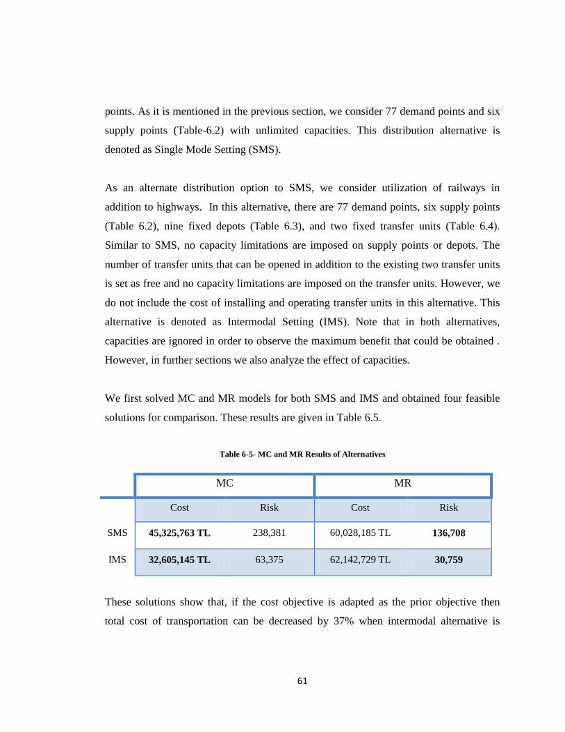
61
points. As it is mentioned in the previous section, we consider 77 demand points and six
supply points (Table-6.2) with unlimited capacities. This distribution alternative is
denoted as Single Mode Setting (SMS).
As an alternate distribution option to SMS, we consider utilization of railways in
addition to highways. In this alternative, there are 77 demand points, six supply points
(Table 6.2), nine fixed depots (Table 6.3), and two fixed transfer units (Table 6.4).
Similar to SMS, no capacity limitations are imposed on supply points or depots. The
number of transfer units that can be opened in addition to the existing two transfer units
is set as free and no capacity limitations are imposed on the transfer units. However, we
do not include the cost of installing and operating transfer units in this alternative. This
alternative is denoted as Intermodal Setting (IMS). Note that in both alternatives,
capacities are ignored in order to observe the maximum benefit that could be obtained .
However, in further sections we also analyze the effect of capacities.
We first solved MC and MR models for both SMS and IMS and obtained four feasible
solutions for comparison. These results are given in Table 6.5.
Table 6-5- MC and MR Results of Alternatives
MC MR
Cost Risk Cost Risk
SMS 45,325,763 TL 238,381 60,028,185 TL 136,708
IMS 32,605,145 TL 63,375 62,142,729 TL 30,759
These solutions show that, if the cost objective is adapted as the prior objective then
total cost of transportation can be decreased by 37% when intermodal alternative is
62
chosen. Similarly, if risk objective is the preferred objective then total risk of fuel
distribution of Turkey can be decreased by 81% by introducing the railroads as an
alternative transportation mode.
Moreover, when these four solutions are compared to each other, we observe that MC
solution of the IMS, which is denoted as MC(IMS), dominates the MR and MC
solutions of SMS. This shows that none of the efficient solutions obtained by SMS can
be an efficient solution when intermodal transportation is adapted. We found the two
extreme solutions for SMS, which are MC(SMS) and MR(SMS) solutions. Since these
solutions are dominated by MC(IMS), other possible efficient solutions of SMS that
would lie in between these two extreme solutions will also be dominated by MC(IMS),
accordingly. The resulting distribution networks of all of the four solutions given in
Table 6.5 are depicted in Figure 6.7.
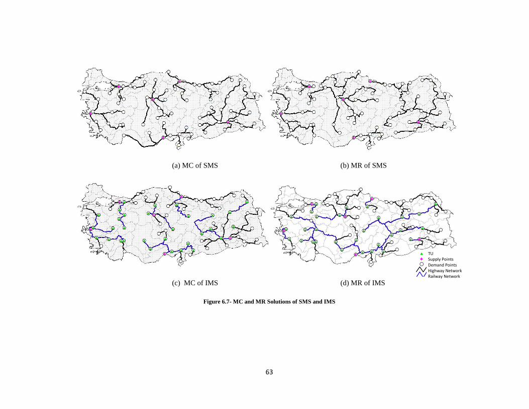
63
(a) MC of SMS (b) MR of SMS
(c) MC of IMS (d) MR of IMS
Figure 6.7- MC and MR Solutions of SMS and IMS
Ilsinir.shpAllturkey.shpBase-mc-rail.shpBase-mc-road.shp
#S Final-cities.shpÑ Supplypoints.shp$ Base-mc-tu.shpTU
Supply Points Demand Points Highway Network Railway Network
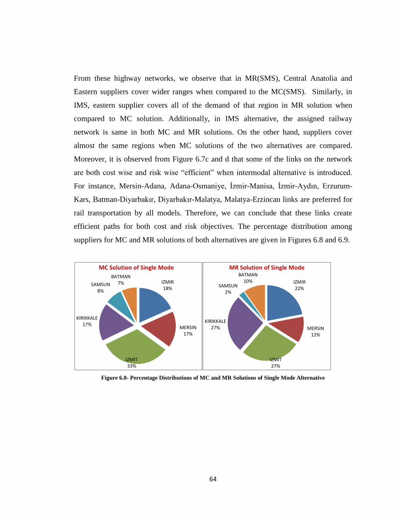
64
From these highway networks, we observe that in MR(SMS), Central Anatolia and
Eastern suppliers cover wider ranges when compared to the MC(SMS). Similarly, in
IMS, eastern supplier covers all of the demand of that region in MR solution when
compared to MC solution. Additionally, in IMS alternative, the assigned railway
network is same in both MC and MR solutions. On the other hand, suppliers cover
almost the same regions when MC solutions of the two alternatives are compared.
Moreover, it is observed from Figure 6.7c and d that some of the links on the network
are both cost wise and risk wise “efficient” when intermodal alternative is introduced.
For instance, Mersin-Adana, Adana-Osmaniye, Ġzmir-Manisa, Ġzmir-Aydın, Erzurum-
Kars, Batman-Diyarbakır, Diyarbakır-Malatya, Malatya-Erzincan links are preferred for
rail transportation by all models. Therefore, we can conclude that these links create
efficient paths for both cost and risk objectives. The percentage distribution among
suppliers for MC and MR solutions of both alternatives are given in Figures 6.8 and 6.9.
Figure 6.8- Percentage Distributions of MC and MR Solutions of Single Mode Alternative
IZMIR 18%
MERSIN 17%
IZMIT 33%
KIRIKKALE 17%
SAMSUN 8%
BATMAN 7%
MC Solution of Single Mode
IZMIR 22%
MERSIN 12%
IZMIT 27%
KIRIKKALE 27%
SAMSUN 2%
BATMAN 10%
MR Solution of Single Mode
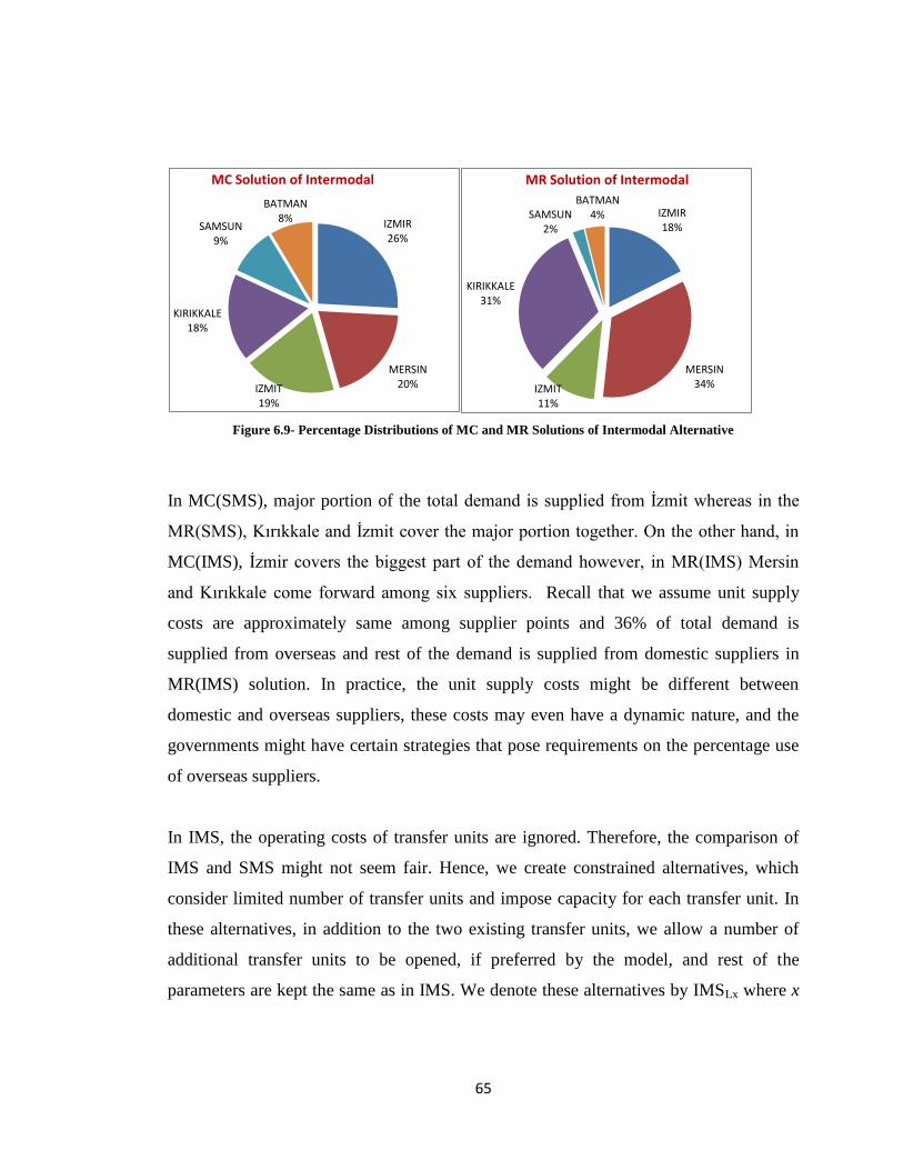
65
Figure 6.9- Percentage Distributions of MC and MR Solutions of Intermodal Alternative
In MC(SMS), major portion of the total demand is supplied from Ġzmit whereas in the
MR(SMS), Kırıkkale and Ġzmit cover the major portion together. On the other hand, in
MC(IMS), Ġzmir covers the biggest part of the demand however, in MR(IMS) Mersin
and Kırıkkale come forward among six suppliers. Recall that we assume unit supply
costs are approximately same among supplier points and 36% of total demand is
supplied from overseas and rest of the demand is supplied from domestic suppliers in
MR(IMS) solution. In practice, the unit supply costs might be different between
domestic and overseas suppliers, these costs may even have a dynamic nature, and the
governments might have certain strategies that pose requirements on the percentage use
of overseas suppliers.
In IMS, the operating costs of transfer units are ignored. Therefore, the comparison of
IMS and SMS might not seem fair. Hence, we create constrained alternatives, which
consider limited number of transfer units and impose capacity for each transfer unit. In
these alternatives, in addition to the two existing transfer units, we allow a number of
additional transfer units to be opened, if preferred by the model, and rest of the
parameters are kept the same as in IMS. We denote these alternatives by IMSLx where x
IZMIR 26%
MERSIN 20% IZMIT
19%
KIRIKKALE 18%
SAMSUN 9%
BATMAN 8%
MC Solution of Intermodal
IZMIR 18%
MERSIN 34% IZMIT
11%
KIRIKKALE 31%
SAMSUN 2%
BATMAN 4%
MR Solution of Intermodal
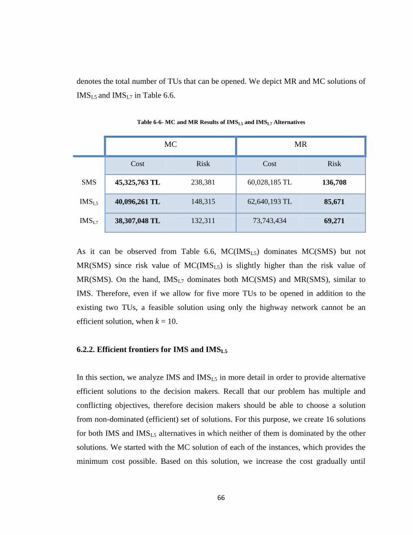
66
denotes the total number of TUs that can be opened. We depict MR and MC solutions of
IMSL5 and IMSL7 in Table 6.6.
Table 6-6- MC and MR Results of IMSL5 and IMSL7 Alternatives
MC MR
Cost Risk Cost Risk
SMS 45,325,763 TL 238,381 60,028,185 TL 136,708
IMSL5 40,096,261 TL 148,315 62,640,193 TL 85,671
IMSL7 38,307,048 TL 132,311 73,743,434 69,271
As it can be observed from Table 6.6, MC(IMSL5) dominates MC(SMS) but not
MR(SMS) since risk value of MC(IMSL5) is slightly higher than the risk value of
MR(SMS). On the hand, IMSL7 dominates both MC(SMS) and MR(SMS), similar to
IMS. Therefore, even if we allow for five more TUs to be opened in addition to the
existing two TUs, a feasible solution using only the highway network cannot be an
efficient solution, when k = 10.
6.2.2. Efficient frontiers for IMS and IMSL5
In this section, we analyze IMS and IMSL5 in more detail in order to provide alternative
efficient solutions to the decision makers. Recall that our problem has multiple and
conflicting objectives, therefore decision makers should be able to choose a solution
from non-dominated (efficient) set of solutions. For this purpose, we create 16 solutions
for both IMS and IMSL5 alternatives in which neither of them is dominated by the other
solutions. We started with the MC solution of each of the instances, which provides the
minimum cost possible. Based on this solution, we increase the cost gradually until
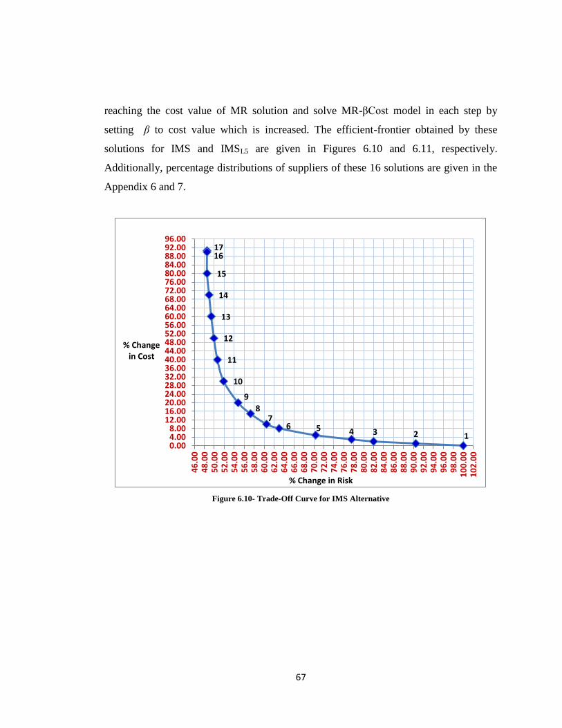
67
reaching the cost value of MR solution and solve MR-βCost model in each step by
setting β to cost value which is increased. The efficient-frontier obtained by these
solutions for IMS and IMSL5 are given in Figures 6.10 and 6.11, respectively.
Additionally, percentage distributions of suppliers of these 16 solutions are given in the
Appendix 6 and 7.
Figure 6.10- Trade-Off Curve for IMS Alternative
17 16
15
14
13
12
11
10
9
8 7
6 5 4 3 2 1 0.00 4.00 8.00
12.00 16.00 20.00 24.00 28.00 32.00 36.00 40.00 44.00 48.00 52.00 56.00 60.00 64.00 68.00 72.00 76.00 80.00 84.00 88.00 92.00 96.00
46
.00
4
8.0
0
50
.00
5
2.0
0
54
.00
5
6.0
0
58
.00
6
0.0
0
62
.00
6
4.0
0
66
.00
6
8.0
0
70
.00
7
2.0
0
74
.00
7
6.0
0
78
.00
8
0.0
0
82
.00
8
4.0
0
86
.00
8
8.0
0
90
.00
9
2.0
0
94
.00
9
6.0
0
98
.00
1
00
.00
1
02
.00
% Change in Cost
% Change in Risk

68
Figure 6.11- Trade-off Curve for IMSL Alternative
In these graphs, x-coordinate corresponds to the percentage reduction in the
transportation risk with respect to the transportation risk imposed by the MC solution.
Similarly, y-coordinate corresponds to the percentage change in the total cost with
respect to the minimum cost obtained by the MC model. As an example, consider Point
6 of Figure 6.10. This point is obtained by solving MR-βCost model where β is equal to
8% more of the optimal MC(IMS) solution. The total cost of this solution is 8% higher
than the minimum cost obtained by MC model whereas the resulting risk saving is 32%
when compared to the total risk of the MC solution.
16
15
14
13
12
11
10
9
8
7 6
5 4 3 2
1 0.00 2.00 4.00 6.00 8.00
10.00 12.00 14.00 16.00 18.00 20.00 22.00 24.00 26.00 28.00 30.00 32.00 34.00 36.00 38.00 40.00 42.00 44.00 46.00 48.00 50.00 52.00 54.00 56.00 58.00
56
.00
58
.00
60
.00
62
.00
64
.00
66
.00
68
.00
70
.00
72
.00
74
.00
76
.00
78
.00
80
.00
82
.00
84
.00
86
.00
88
.00
90
.00
92
.00
94
.00
96
.00
98
.00
10
0.0
0
10
2.0
0
% Change in Cost
% Change in Risk
69
From the perspective of a decision maker, whose prior objective is cost minimization
while regarding also the societal risk, Point 6 could be an acceptable solution since 8%
increment on the cost results a significant risk saving. Additionally, from this point
forward, increasing cost does not provide satisfactory risk saving with respect to Point 6.
6.2.3. Effects of the number of Transfer Units
In this section, we analyze the effect of opening different number of transfer units by
changing the parameter about operating transfer units from perspective of a decision
maker described in the previous section. As mentioned before, in the current system,
carriers mostly prefer distributing the fuel by using only trucks, which does not require
the usage of transfer units. However, when transportation with railways is introduced as
an alternative, depots and transfer units become crucial since transfer between modes
could only be available via depots or transfer units.
Installation of new depots are both costly and require strategic decisions to be made by
carrier companies and the respective governmental authorities. Therefore, we do not
allow for opening new depots in our numerical analysis, however we allow for opening
new TUs. We note that opening TUs are less costly and require decisions at the tactical
level. Nevertheless, we do not explicitly incorporate the installation and operating costs
of TUs in our models, but instead, we observe the benefit of opening new TUs in terms
of cost and risk and propose that the decision maker should make a decision by resolving
the tradeoff between the benefits obtained by opening new TUs and their corresponding
installation and operating costs.
For this purpose, by taking a decision maker for whom the solution of MR-βCost
problem where β is equal to 8% more of MC(IMS) is the preferred solution as a
reference point, we solve this problem by imposing different upper bound values on the
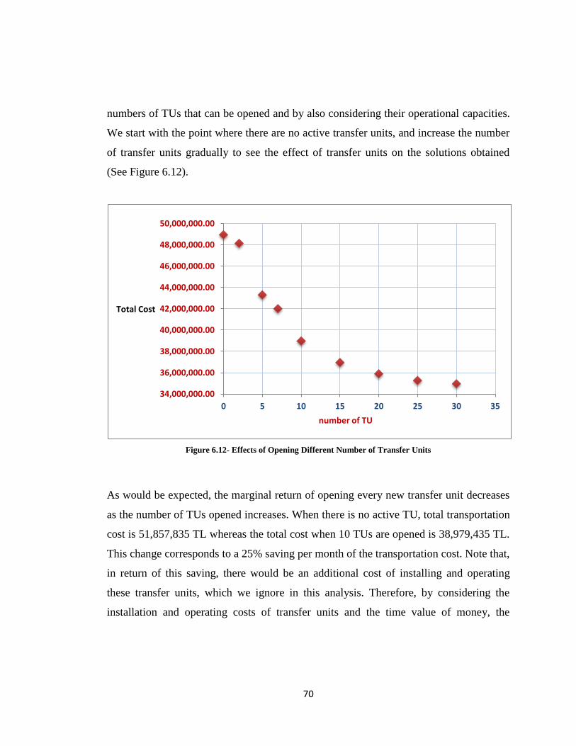
70
numbers of TUs that can be opened and by also considering their operational capacities.
We start with the point where there are no active transfer units, and increase the number
of transfer units gradually to see the effect of transfer units on the solutions obtained
(See Figure 6.12).
Figure 6.12- Effects of Opening Different Number of Transfer Units
As would be expected, the marginal return of opening every new transfer unit decreases
as the number of TUs opened increases. When there is no active TU, total transportation
cost is 51,857,835 TL whereas the total cost when 10 TUs are opened is 38,979,435 TL.
This change corresponds to a 25% saving per month of the transportation cost. Note that,
in return of this saving, there would be an additional cost of installing and operating
these transfer units, which we ignore in this analysis. Therefore, by considering the
installation and operating costs of transfer units and the time value of money, the
34,000,000.00
36,000,000.00
38,000,000.00
40,000,000.00
42,000,000.00
44,000,000.00
46,000,000.00
48,000,000.00
50,000,000.00
0 5 10 15 20 25 30 35
Total Cost
number of TU
71
decision maker should estimate the total time needed to recoup this investment and
select the number of transfer units to operate with, accordingly.
6.2.4. Effects of highway accident rate
As explained in Section 6.1, we are not able to estimate the highway accident rate
satisfactorily but set the highway accident rate as 10 times greater than the railway
accident rate based on common sense. Nevertheless, setting k = 10 might be an over
estimation. Therefore, we analyze the impact of different values of this parameter on the
solutions obtained while assessing the benefits of intermodal distribution system over
the single mode system.
As stated in the Section 6.2.1, when k = 10, MC(IMS) dominates MR(SMS) and
MC(SMS). This implies that, if k = 10, none of the efficient solutions obtained for the
design of fuel distribution system of Turkey could consist of only highway mode of
transportation. This property is a strong one showing the pure benefit of introducing
multi-modal transportation system for Turkey’s fuel distribution system.
Considering that that k = 10 might be an overestimation, we reduced k value gradually to
observe until which value of k the same property still holds. We observe that even if k is
equal to 0.8, meaning that the accident rate of trains is higher than that of trucks, a
distribution system composed of only highway transportation cannot be in the efficient
set of solutions (See Table 6.7). When k is set to 0.7, this property no longer holds.
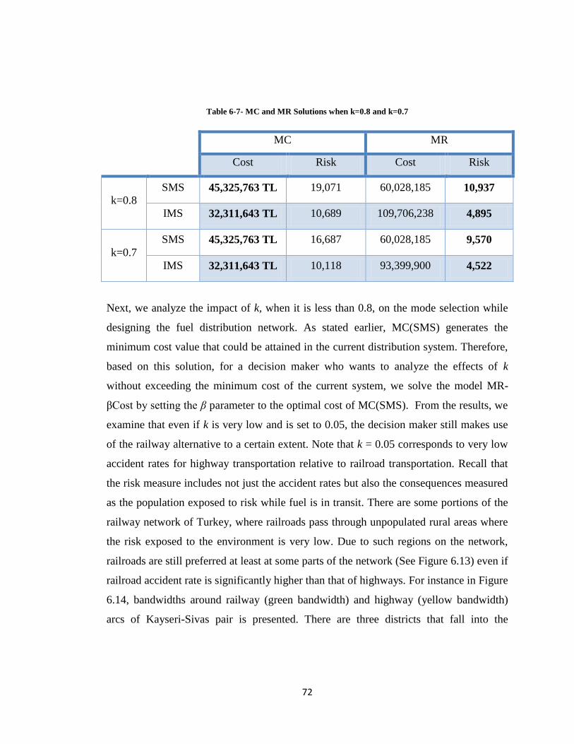
72
Table 6-7- MC and MR Solutions when k=0.8 and k=0.7
MC MR
Cost Risk Cost Risk
k=0.8
SMS 45,325,763 TL 19,071 60,028,185 10,937
IMS 32,311,643 TL 10,689 109,706,238 4,895
k=0.7
SMS 45,325,763 TL 16,687 60,028,185 9,570
IMS 32,311,643 TL 10,118 93,399,900 4,522
Next, we analyze the impact of k, when it is less than 0.8, on the mode selection while
designing the fuel distribution network. As stated earlier, MC(SMS) generates the
minimum cost value that could be attained in the current distribution system. Therefore,
based on this solution, for a decision maker who wants to analyze the effects of k
without exceeding the minimum cost of the current system, we solve the model MR-
βCost by setting the β parameter to the optimal cost of MC(SMS). From the results, we
examine that even if k is very low and is set to 0.05, the decision maker still makes use
of the railway alternative to a certain extent. Note that k = 0.05 corresponds to very low
accident rates for highway transportation relative to railroad transportation. Recall that
the risk measure includes not just the accident rates but also the consequences measured
as the population exposed to risk while fuel is in transit. There are some portions of the
railway network of Turkey, where railroads pass through unpopulated rural areas where
the risk exposed to the environment is very low. Due to such regions on the network,
railroads are still preferred at least at some parts of the network (See Figure 6.13) even if
railroad accident rate is significantly higher than that of highways. For instance in Figure
6.14, bandwidths around railway (green bandwidth) and highway (yellow bandwidth)
arcs of Kayseri-Sivas pair is presented. There are three districts that fall into the
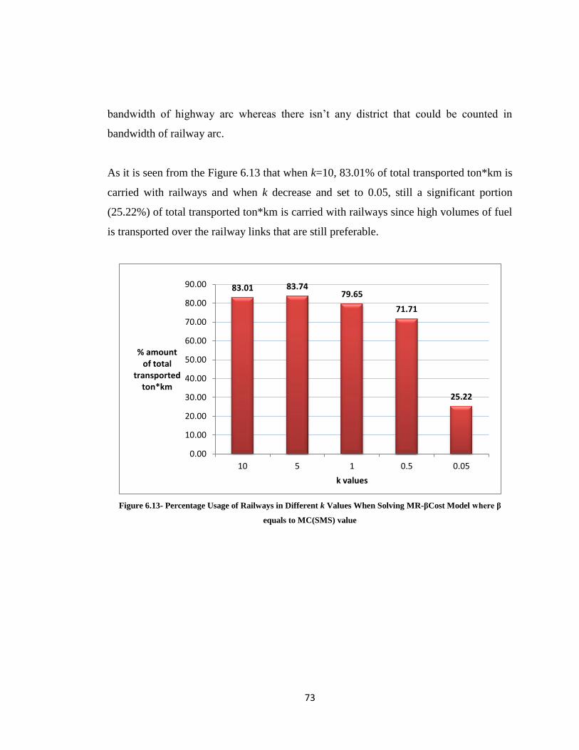
73
bandwidth of highway arc whereas there isn’t any district that could be counted in
bandwidth of railway arc.
As it is seen from the Figure 6.13 that when k=10, 83.01% of total transported ton*km is
carried with railways and when k decrease and set to 0.05, still a significant portion
(25.22%) of total transported ton*km is carried with railways since high volumes of fuel
is transported over the railway links that are still preferable.
Figure 6.13- Percentage Usage of Railways in Different k Values When Solving MR-βCost Model where β
equals to MC(SMS) value
83.01 83.74 79.65
71.71
25.22
0.00
10.00
20.00
30.00
40.00
50.00
60.00
70.00
80.00
90.00
10 5 1 0.5 0.05
% amount of total
transported ton*km
k values
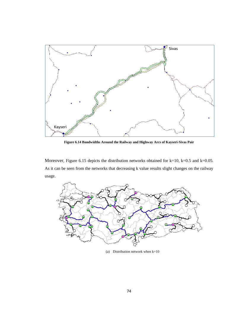
74
Figure 6.14 Bandwidths Around the Railway and Highway Arcs of Kayseri-Sivas Pair
Moreover, Figure 6.15 depicts the distribution networks obtained for k=10, k=0.5 and k=0.05.
As it can be seen from the networks that decreasing k value results slight changes on the railway
usage.
(a) Distribution network when k=10
Sivas
Kayseri
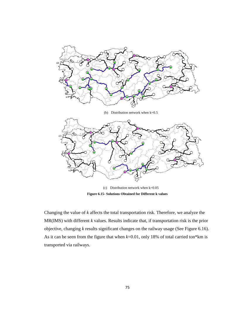
75
(b) Distribution network when k=0.5
(c) Distribution network when k=0.05
Figure 6.15- Solutions Obtained for Different k values
Changing the value of k affects the total transportation risk. Therefore, we analyze the
MR(IMS) with different k values. Results indicate that, if transportation risk is the prior
objective, changing k results significant changes on the railway usage (See Figure 6.16).
As it can be seen from the figure that when k=0.01, only 18% of total carried ton*km is
transported via railways.
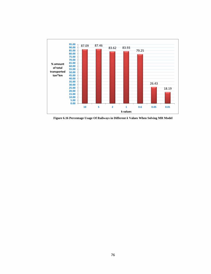
76
Figure 6.16 Percentage Usage Of Railways in Different k Values When Solving MR Model
87.09 87.46 83.62 83.93
79.25
26.43
18.19
0.00 5.00
10.00 15.00 20.00 25.00 30.00 35.00 40.00 45.00 50.00 55.00 60.00 65.00 70.00 75.00 80.00 85.00 90.00 95.00
10 5 2 1 0.6 0.05 0.01
% amount of total
transported ton*km
k values
77
Chapter 7
Conclusion
Hazardous materials transportation problem is an important problem that should be
handled with extreme care since it is different from regular freight transportation as
hazardous materials may harm to people, property or environment when an incident
occurs. In this study, we focused on the fuel products, which belong to flammable and
combustible liquids class of the hazardous materials classes.
As explained in the earlier chapters, fuel products are procured by fuel companies from
supplier points in the current fuel distribution system of Turkey. After procurement, fuel
is transferred to the transfer units or storage terminals of companies in order to charge
the fuel products to road tankers. Finally, charged products are distributed via highways
among the customer points. Since Turkey has a dense highway network, most of the
leader fuel companies prefer to use road tankers for distribution. However, railway
transportation is another favorable alternative with respect to advantages explained in
78
Chapter-3. We analyze implementing a combination of railway and highway
transportation alternatives which is referred as rail-truck intermodal transportation.
“Risk” is considered as a crucial aspect of the hazardous material transportation
problem. There are many studies deal with the risk modeling over highways in the
literature. However, only a few recent ones focused on railway risk modeling. We adapt
the risk model conducted by Glickman et al. (2007) and modify the model to our case by
making a few changes. We collected all the needed data specialized on Turkey. Hence,
calculating the risk values by the proposed model is one of the contributions of this
study.
We propose a mathematical model whose aim is to decide on the following three
questions: where to open transfer units, how to route fuel products from suppliers to
customer by using which transportation mode, and which supplier covers how much
demand. In this model, we define supplied amounts as a decision variable in order to
observe the optimal coverage of each supplier. Thus, model provides opportunity to
compare the required capacity and actual capacity of the suppliers.
Our model considers two conflicting objectives of intermodal fuel transportation
problem, which are total cost and transportation risk. Based on these objectives, we
create three variances of the base model. First one is MC model, whose objective is to
minimize total cost of transportation. Second one is MR model, whose objective is to
minimize total transportation risk and last one is MR-βCost model, which considers the
risk function as the objective and uses the cost objective as a constraint.
Initially, we compare intermodal transportation alternative with the single mode
alternative by using MC and MR models initially. Solutions indicate that intermodal
alternative, which uses railways in conjunction with the highways, create significant
79
reductions on both transportation risk and cost. In fact, it is observed that IMS
alternative always provides better solutions under the condition that there is no
limitation on the transfer units.
As mentioned before, transfer units are important components of the intermodal
transportation system. Therefore, we conduct an analysis by changing the number of
transfer units to be opened. Results show that under the given settings opening 10
transfer units create 25% monthly reduction on the total transportation cost when
compared to the transportation cost of SMS in which there are no active transfer units in
service (See Figure 6.12). Moreover, we analyze the effects of highway accident rate by
changing the coefficient k. Even if we reduce the k value to 0.05, both MR-0.8Cost and
MR solutions still prefer to use railways (See Figure 6.13 and 15).
In this study, we assumed that the fuel distribution system is directed by a centralized
management. However, if we make these analyses for each fuel company separately, the
results of the numerical analyses might change. In our railway risk model, we justify that
the total number of rail wagons that carry fuel products greater or equal to 10. If these
analyses make for each company, the railway risk model and these assumptions should
be revised accordingly.
Additionally, we make all of these analysis based on the current fuel distribution system
in Turkey. As explained in Chapter 3, railway network is very sparse when compared to
highways. Therefore, there are limited route alternatives if a fuel company prefers to
carry its fuel products by using only railways. Moreover, there are some regulations,
which limit the use of the railway network for fuel companies such as leasing limitations
for locomotives and scheduling constraints. Nevertheless, by this study we observe that
using railways in conjunction with highways results significant reductions on both
transportation risk and cost so the distribution system become more efficient in both

80
perspectives. In recent future, if all of the limitations that affect the usage of railways
for fuel transportation are relaxed, we show that rail-truck intermodal transportation of
fuel products will be an applicable and efficient way for fuel companies.
81
BIBLIOGRAPHY Abkowitz, M. D., Lepofsky, M., & Cheng, P. (1992). Selecting Criteria for Designating
Hazardous Materials Highway Routes. Transportation Research Record 1333 , 30-35.
Alp, E. (1995). Risk-based Transportation Planning Practice: Overall Methodology and A Case
Example. INFOR (1) , 4-19.
Alumur, S., & Kara, B. (2007). A new model for the hazardous waste location-routing problem.
Computers & Operations Research , 1406–1423.
Arnold, P., Peeters, D., & Thomas, I. (2004). Modelling a rail/road intermodal transportation
system. Transportation Research Part E 40 , 255–270.
Bontekoning, Y., Macharis, C., & Trip, J. ((2004). Is a new applied transportation research field
emerging?–A review of intermodal rail–truck freight transport literature. Transportation
Research , 1–34.
Bonvicini, S., Leonelli, P., & Spadoni, G. (1998). Risk Analysis of Hazardous Materials
Transportation: Evaluating Uncertainty by Means of Fuzzy Logic. Journal of Hazardous
Materials 62(1) , 59-74.
Boysen, N., Fliedner, M., & Kellner, M. (2010). Determining fixed crane areas in rail–rail
transshipment yards. Transportation Research Part E 46 , 1005–1016.
Brown, D., Policastro, A., Dunn, W., Carhard, R., & Lazaro, M. Development of the initial
isolation and protective action distances for the 2000 Emergency Response Guidebook. Decision
and Information Sciences Division, Argonne National Laboratory.
Browna, D. F., & Dunn, W. E. (2007). Application of A Quantitative Risk Assessment Method to
Emergency Response Planning. Computers & Operations Research 34 , 1243-1265.
Bubbico, R., Ferrari, C., & Mazza, B. (2000). Risk analysis of LPG transport by road and rail.
Journal of Loss Prevention in the Process Industries 13 , 27-31.
Cappanera, P., Galloa, G., & Maffioli, F. (2004). Discrete facility location and routing of
obnoxious activities. Discrete Applied Mathematics , 3 – 28.
Caramia, M., & Guerriero, F. (2009). Aheuristic approach to long-haul freight transportation with
multiple objective functions. Omega 37 , 600 – 614.
82
Caris, A., & Janssens, G. (2009). A local search heuristic for the pre- and end- haulage of
intermodal container terminals. Computers &Operations Research 36 , 2763-2772.
Chang, T.-S. (2008). Best routes selection in international intermodal networks. Computers &
Operations Research , 2877 – 2891.
Covello, V. T., & Merkhofer, M. W. (1993). Risk Assessment Methods: Approaches for
Assessing Health and Environmental Risks. NY: Plenum Press.
(2007). Intermodal Transportation. In T. G. Crainic, & K. H. Kim, Handbooks in Operations
Research and Management Science, Transportation (Vol. 14, pp. 467-537). North-Holland.
EMRA. (2010). Retrieved from Energy Market Regulatory Authority.
Erkut, E., & Verter, V. (1995). Hazardous Materials Logistics. In Z. Drezner (Ed.), Facility
Location: A Survey of Applications and Methods. Springer-Verlag.
Erkut, E., & Verter, V. (1998). Modeling Of Transport Risk For Hazardous Materials. Operations
Research 46 , 625-642.
Erkut, E., Tjandra, S. A., & Verter, V. (2007). Hazardous Materials Transportation. In C.
Barnhart, & G. Laporte, Handbooks in Operations Research and Management Science,
Transportation (Vol. 14, pp. 539-611). North-Holland.
GDH. (2010). Retrieved from General Directorate of Highways Statistics:
http://www.kgm.gov.tr/Sayfalar/KGM/SiteEng/Root/Statistics.aspx
Giannikos, I. (1998). A multiobjective programming model for locating treatment sites and
routing hazardous wastes. European Journal of Operational Research , 333-342.
Glickman, T. S., Erkut, E., & Zschocke, M. S. (2007). The Cost and Risk Impacts of Rerouting
Railroad Shipments of Hazardous Materials. Accident Analysis and Prevention 39 , 1015–1025.
Helender, M. E., & Melachrinoudis, E. (1997). Facility location and reliable route planning in
hazardous material transportation. Transportation Science 31 , 216-226.
Jenness, J. (2003). Jenness Enterprises. Retrieved from
http://www.jennessent.com/arcview/within_distance.htm
Justice, E. (1996). Optimization of chassis reallocation in doublestack container transportation
systems (rail cars, scheduling). Ph.D. thesis, University of Arkansas.
Lei, T. L., & Church, R. L. (2011). Locating short-term empty-container storage facilities to
support port operations: A user optimal approach. Transportation Research Part E 47 , 738–754.
83
List, G., & Mirchandani, P. (1991). An integrated network/planar multiobjective model for
routing and siting for hazardous materials. Transportation Science 25 (2) , 146-156.
Macharis, C., & Bontekoning, Y. (2004). Opportunities for OR in intermodal freight transport
research: A review. European Journal of Operational Research 153 , 400-416.
Milazzo, M., Lisi, R., Maschio, G., & Anto, G. (2002). HazMat Transport Through Messina
Town: From Risk Analysis Suggestions for Improving Territorial Safety. Journal of Loss
Prevention in the Process Industries 15 , 347-356.
Min, H. (1991). International intermodal choices via chance-constrained goal programming.
Transportation Research 25 A , 351–362.
Moccia, L., Cordeau, J.-F., Laporte, G., Ropke, S., & Valentini, M. P. (2011). Modeling and
solving a multimodal transportation problem with flexible-time and scheduled services. Networks
57(1) , 53–68.
NHTSA. (2009). Retrieved from National Highway Traffic Safety Administration.
PETDER. (2010). http://www.petder.org.tr.
ReVelle, C., Cohon, J., & Shobrys, D. (1991). Simultaneous Siting and Routing in the Disposal
of Hazardous Hazardous Wastes. Transportation Science 25 , 138-145.
Sivakumar, R. A., Batta, R., & Karwan, M. H. (1995). A Multiple Route Conditional Risk Model
for Transporting. INFOR 33 , 20-33.
Sivakumar, R. A., Batta, R., & Karwan, M. H. (1993). A Network-based Model for Transporting
Extremely Hazardous Materials. Operations Research Letters 13 , 85-93.
Taylor, G. D., Broadstreet, F., Meinert, T. S., & Usher, J. S. (2002). An analysis of intermodal
ramp selection methods. Transportation Research Part E 38 , 117–134.
TSR. (2009). Retrieved from Turkish State Railways Annual Statistics, 2005-2009.
TSR. (2011). Retrieved from Research Planning & Coordination Department.
TUIK. (2010). Retrieved from Traffic Accident Statistics-Road.
U.S. Department of Transportation. (2011). Retrieved from http://www.dot.gov/
U.S. Department of Transportation. (2011). Retrieved from 2011 Hazmat Summary by
Hazardous Materials Class, Pipeline and Hazardous Materials Safety Administration, Office of
Hazardous Material Safety.
Verma, M. (2009). A cost and expected consequence approach to planning and managing railroad
transportation of hazardous materials. Transportation Research Part D 14 , 300–308.
84
Verma, M., & Verter, V. (2010). A lead-time based approach for planning rail–truck intermodal
transportation of dangerous goods. European Journal of Operational Research 202 , 696–706.
Verma, M., & Verter, V. (2007). Railroad transportation of dangerous goods: Population
exposure to airborne toxins. Computers & Operations Research 34 , 1287–1303.
Zhang, J., Hodgson, J., & Erkut, E. (2000). Using GIS to Assess the Risks of Hazardous
Materials Transport in Networks. European Journal of Operational Research 121 , 316-329.
Zhang, R., Yun, W. Y., & Moon, I. K. (2011). Modeling and optimization of acontainer drayag
eproblem with resource constraints. Production Economics 133 , 351–359.
Zografos, K. G., & Samara, S. (1990). Combined location-routing model for hazardous waste
transportation and disposal. Transportation Research Record 1245 , 52-59.
85
APPENDIX
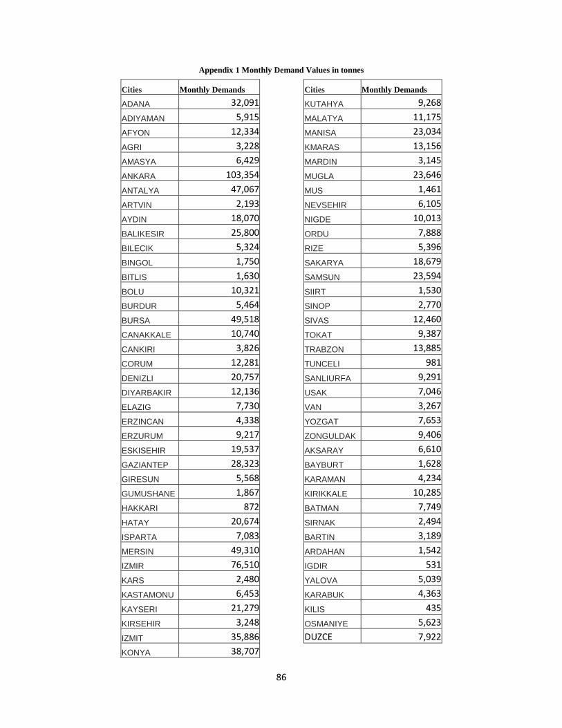
86
Appendix 1 Monthly Demand Values in tonnes
Cities Monthly Demands
Cities Monthly Demands
ADANA 32,091
KUTAHYA 9,268
ADIYAMAN 5,915
MALATYA 11,175
AFYON 12,334
MANISA 23,034
AGRI 3,228
KMARAS 13,156
AMASYA 6,429
MARDIN 3,145
ANKARA 103,354
MUGLA 23,646
ANTALYA 47,067
MUS 1,461
ARTVIN 2,193
NEVSEHIR 6,105
AYDIN 18,070
NIGDE 10,013
BALIKESIR 25,800
ORDU 7,888
BILECIK 5,324
RIZE 5,396
BINGOL 1,750
SAKARYA 18,679
BITLIS 1,630
SAMSUN 23,594
BOLU 10,321
SIIRT 1,530
BURDUR 5,464
SINOP 2,770
BURSA 49,518
SIVAS 12,460
CANAKKALE 10,740
TOKAT 9,387
CANKIRI 3,826
TRABZON 13,885
CORUM 12,281
TUNCELI 981
DENIZLI 20,757
SANLIURFA 9,291
DIYARBAKIR 12,136
USAK 7,046
ELAZIG 7,730
VAN 3,267
ERZINCAN 4,338
YOZGAT 7,653
ERZURUM 9,217
ZONGULDAK 9,406
ESKISEHIR 19,537
AKSARAY 6,610
GAZIANTEP 28,323
BAYBURT 1,628
GIRESUN 5,568
KARAMAN 4,234
GUMUSHANE 1,867
KIRIKKALE 10,285
HAKKARI 872
BATMAN 7,749
HATAY 20,674
SIRNAK 2,494
ISPARTA 7,083
BARTIN 3,189
MERSIN 49,310
ARDAHAN 1,542
IZMIR 76,510
IGDIR 531
KARS 2,480
YALOVA 5,039
KASTAMONU 6,453
KARABUK 4,363
KAYSERI 21,279
KILIS 435
KIRSEHIR 3,248
OSMANIYE 5,623
IZMIT 35,886
DUZCE 7,922
KONYA 38,707
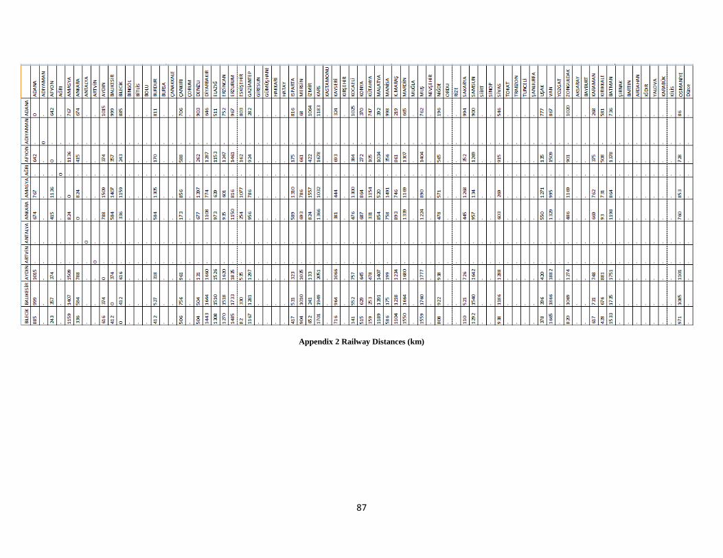
87
Appendix 2 Railway Distances (km)
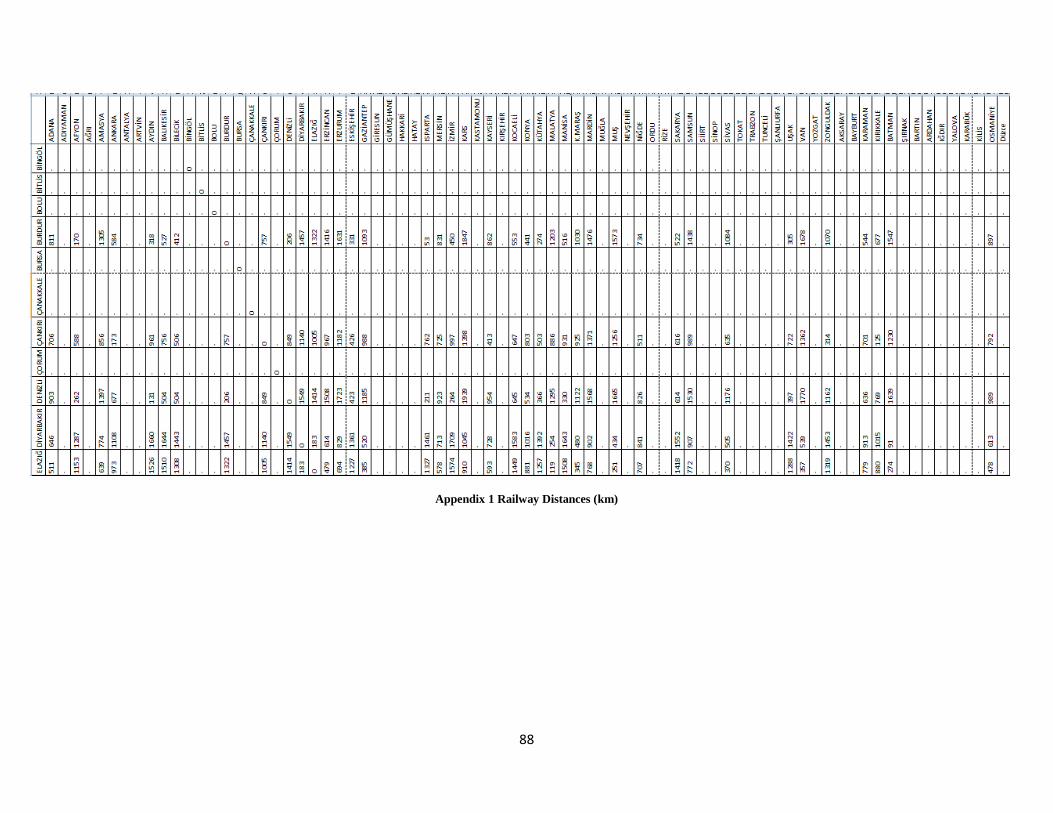
88
Appendix 1 Railway Distances (km)
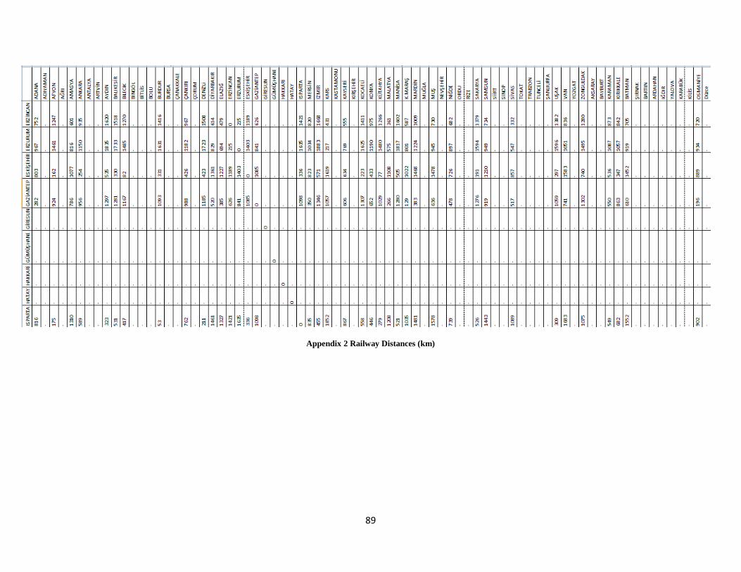
89
Appendix 2 Railway Distances (km)
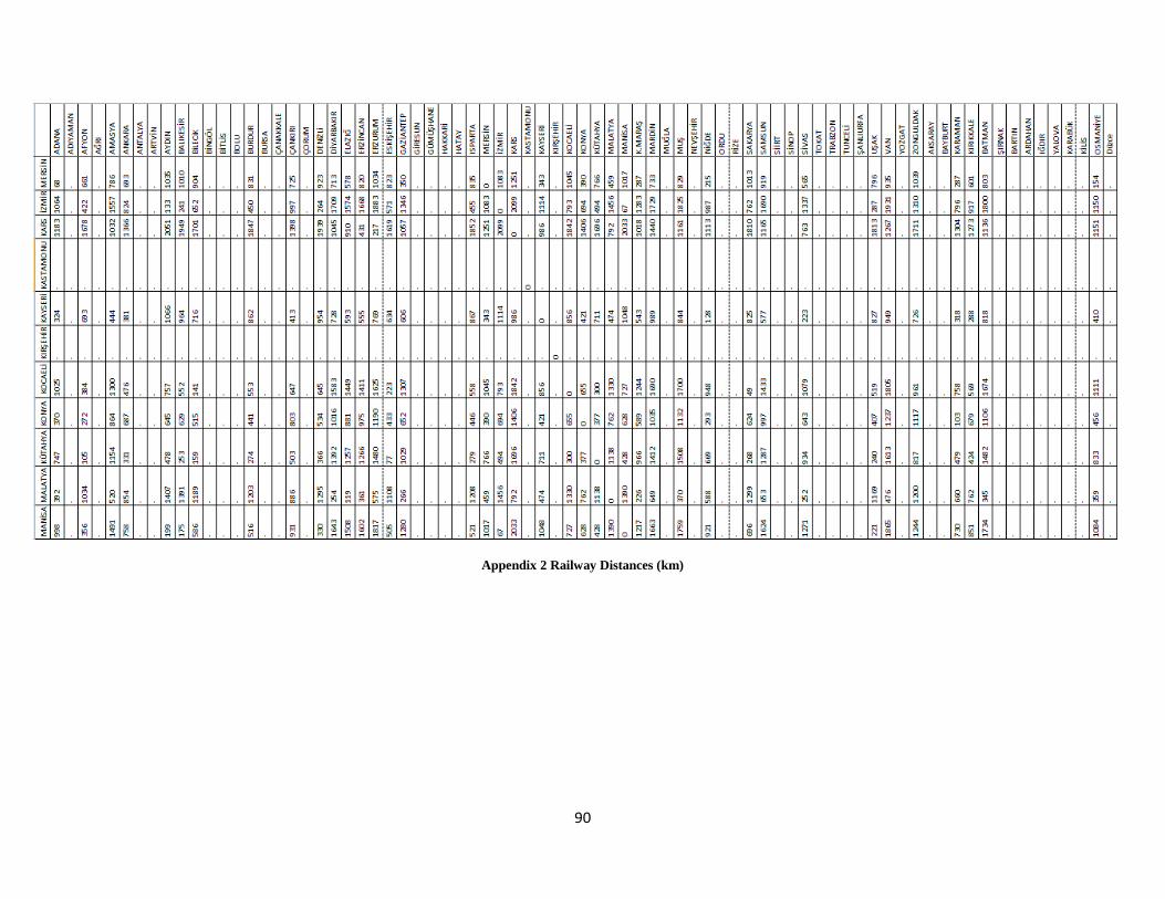
90
Appendix 2 Railway Distances (km)
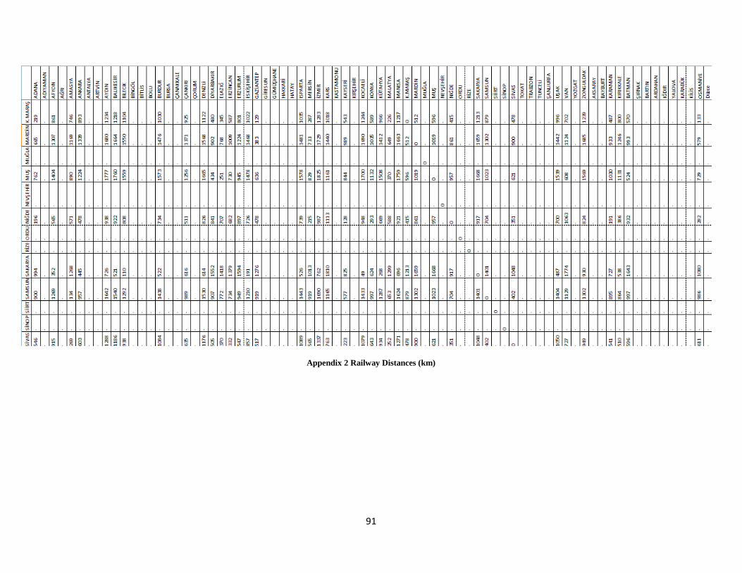
91
Appendix 2 Railway Distances (km)
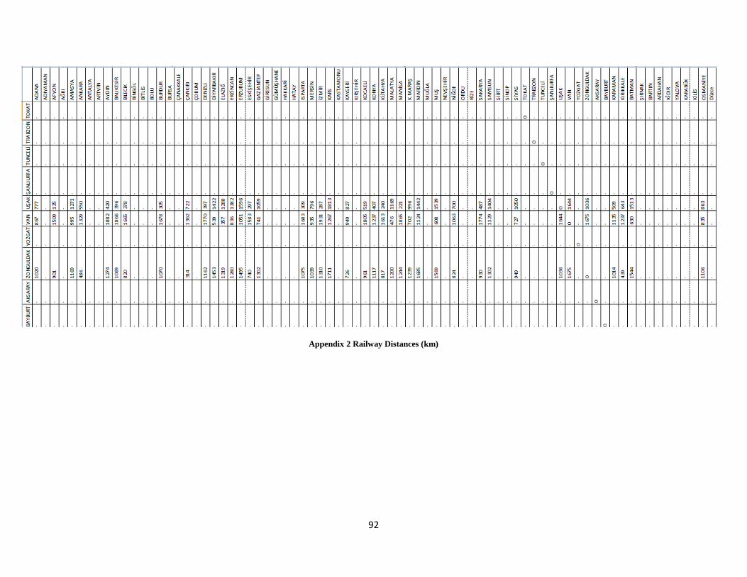
92
Appendix 2 Railway Distances (km)
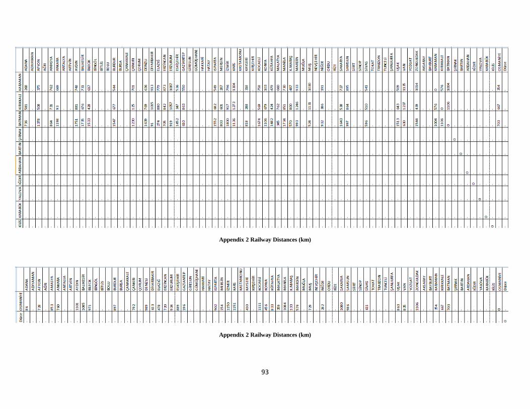
93
Appendix 2 Railway Distances (km)
Appendix 2 Railway Distances (km)
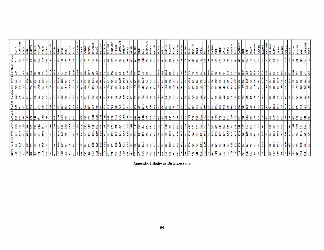
94
Appendix 3 Highway Distances (km)
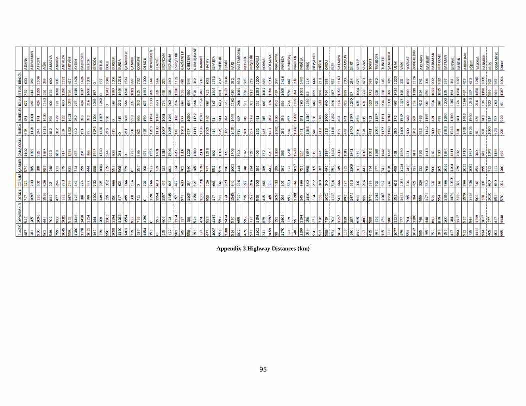
95
Appendix 3 Highway Distances (km)
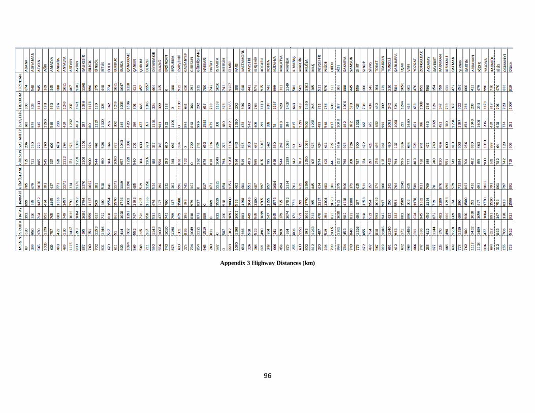
96
Appendix 3 Highway Distances (km)
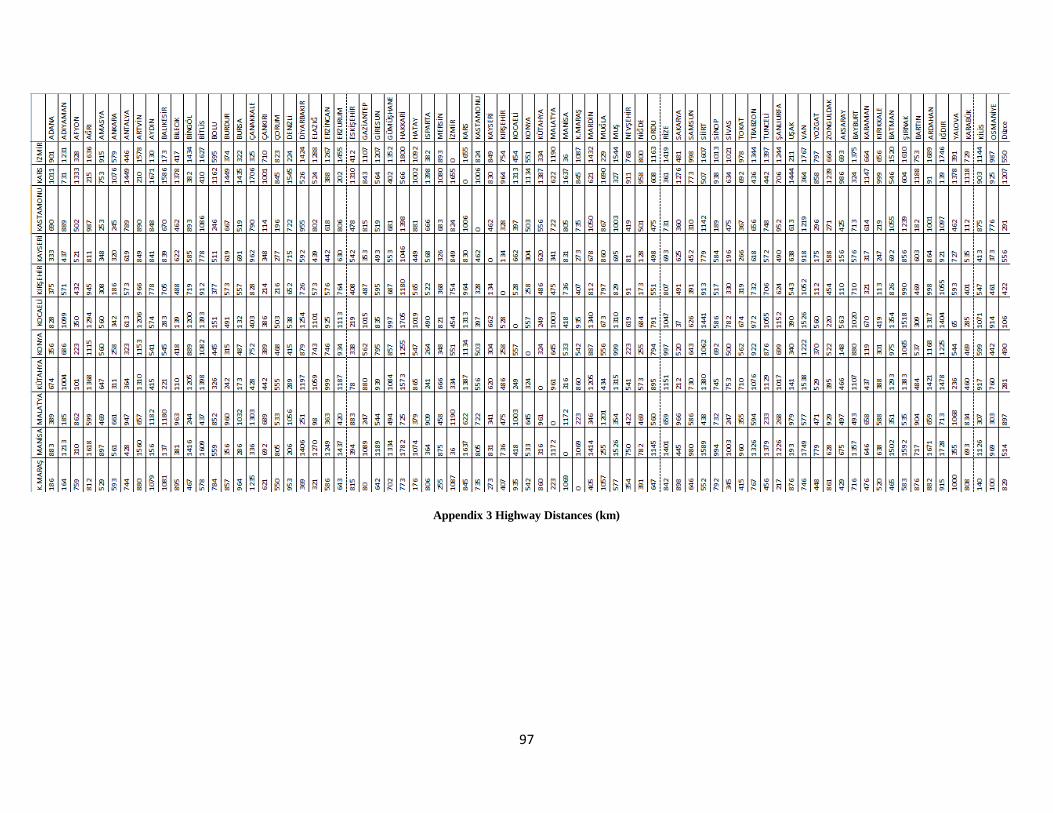
97
Appendix 3 Highway Distances (km)
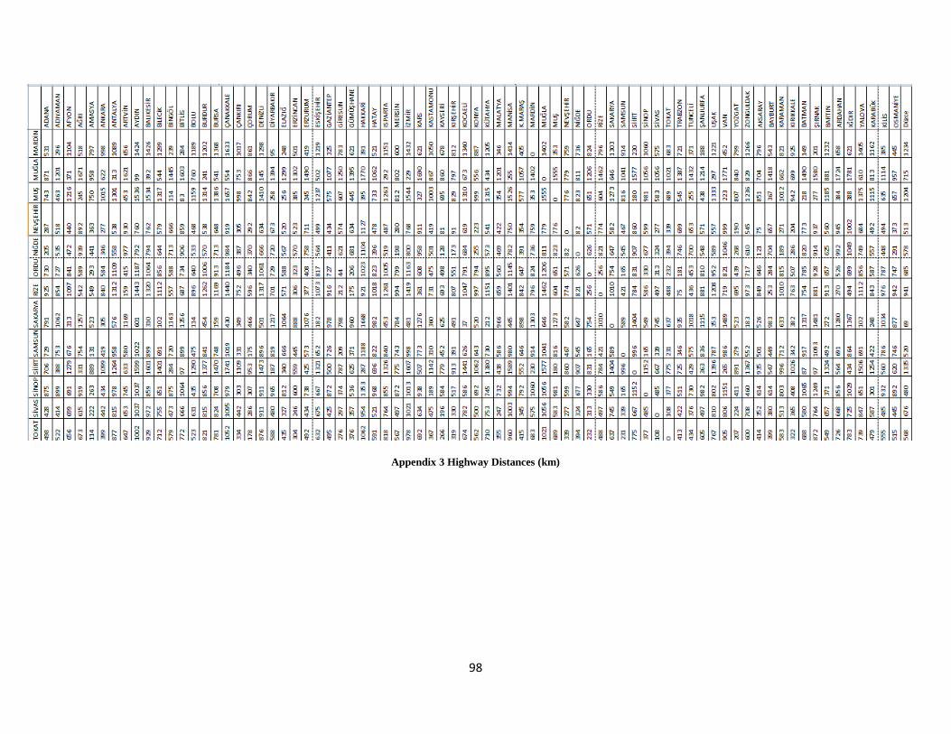
98
Appendix 3 Highway Distances (km)
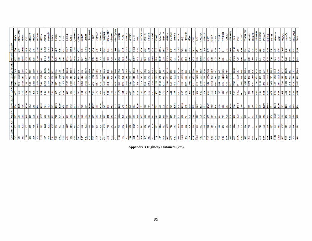
99
Appendix 3 Highway Distances (km)
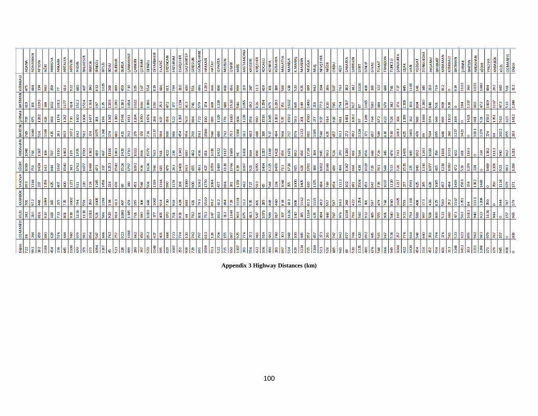
100
Appendix 3 Highway Distances (km)
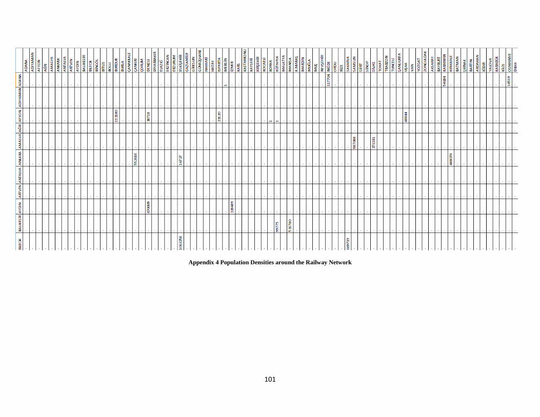
101
Appendix 4 Population Densities around the Railway Network
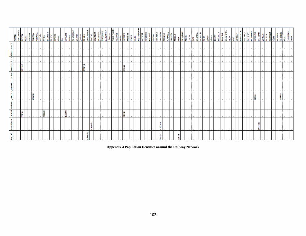
102
Appendix 4 Population Densities around the Railway Network
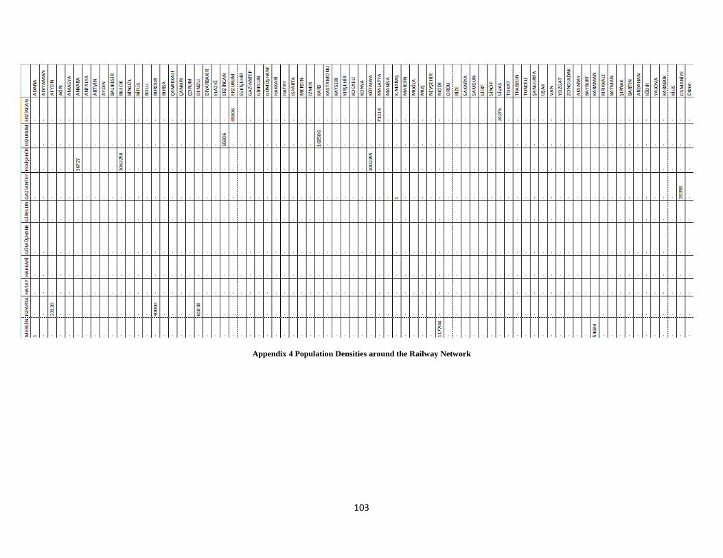
103
Appendix 4 Population Densities around the Railway Network
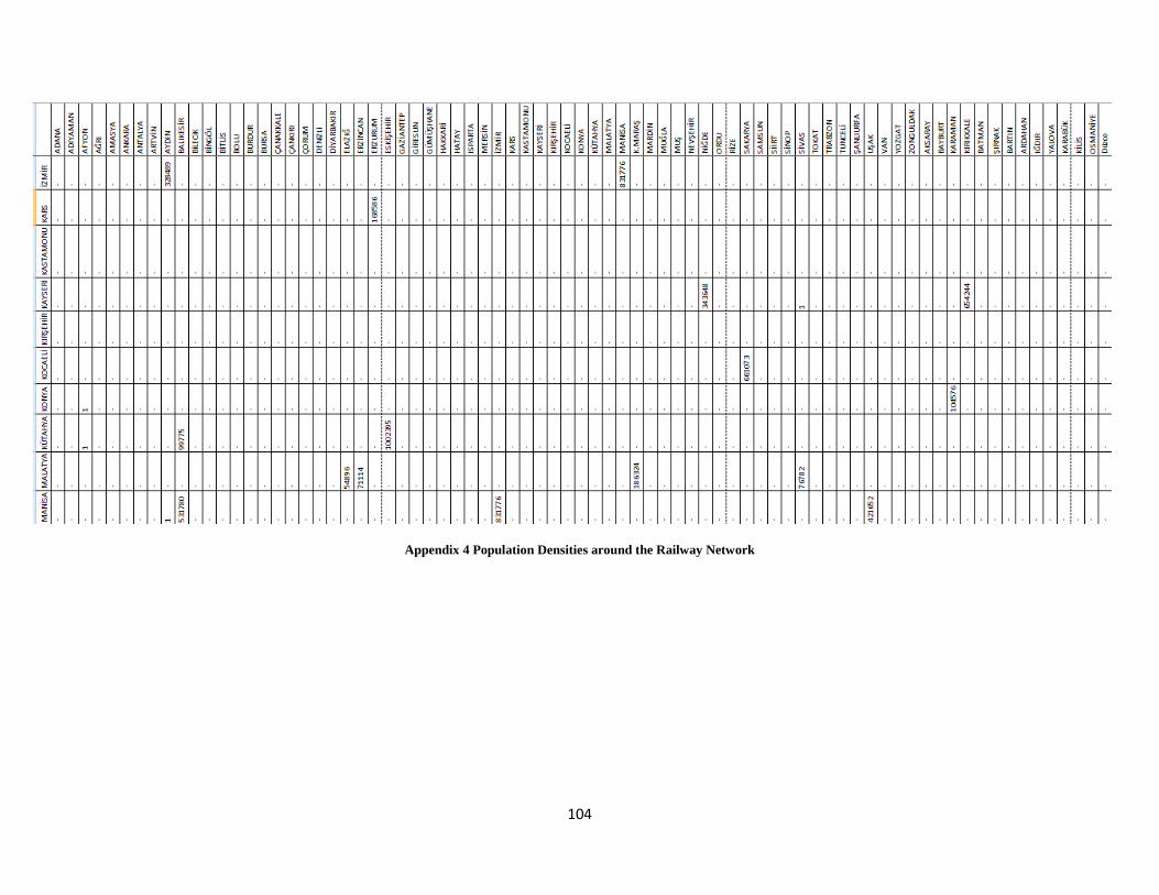
104
Appendix 4 Population Densities around the Railway Network
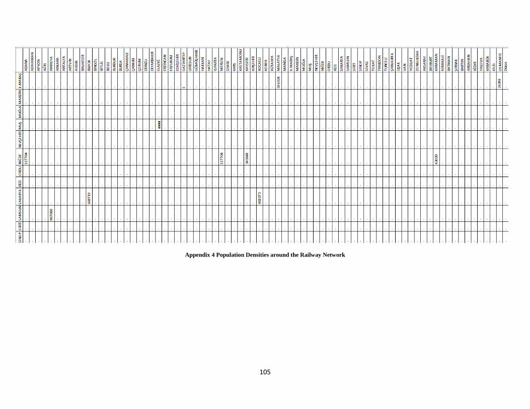
105
Appendix 4 Population Densities around the Railway Network
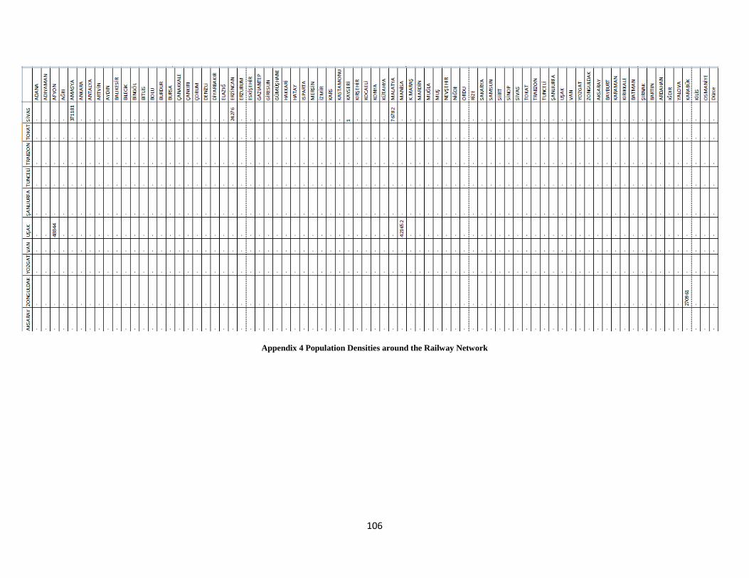
106
Appendix 4 Population Densities around the Railway Network
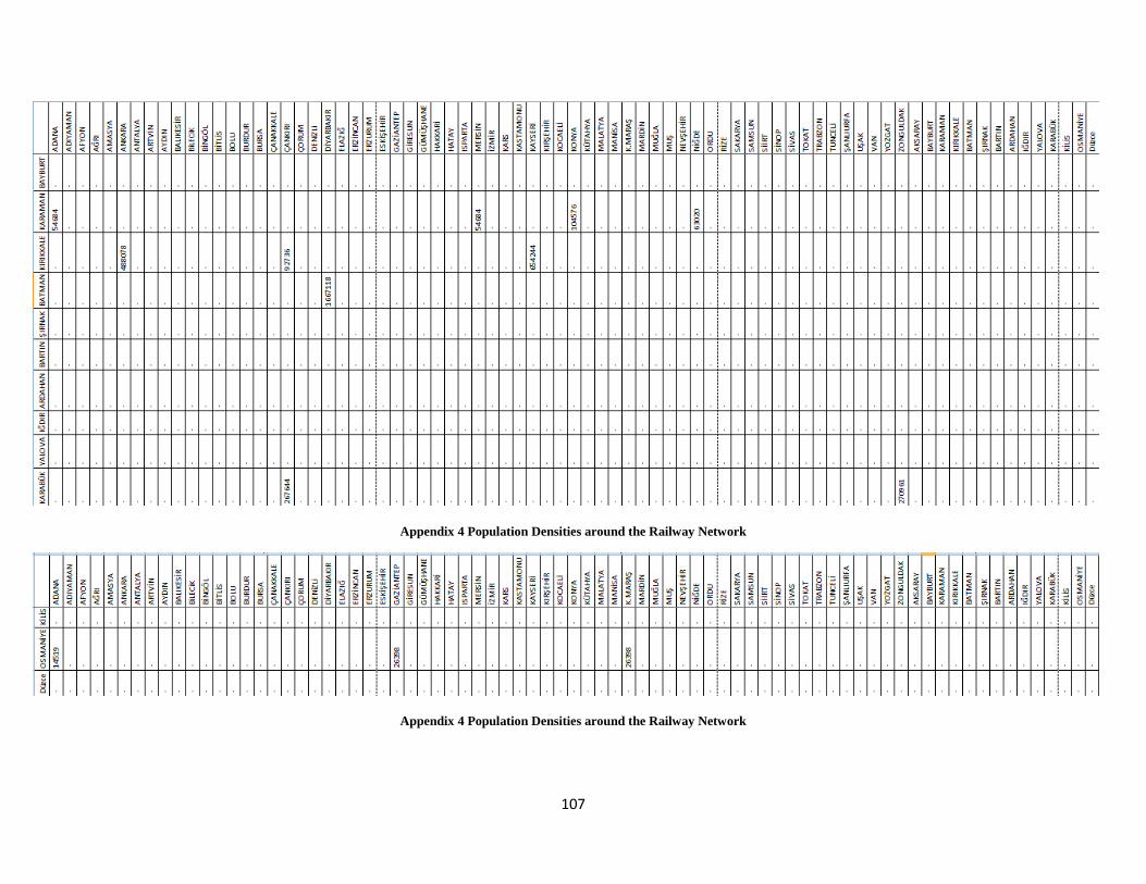
107
Appendix 4 Population Densities around the Railway Network
Appendix 4 Population Densities around the Railway Network
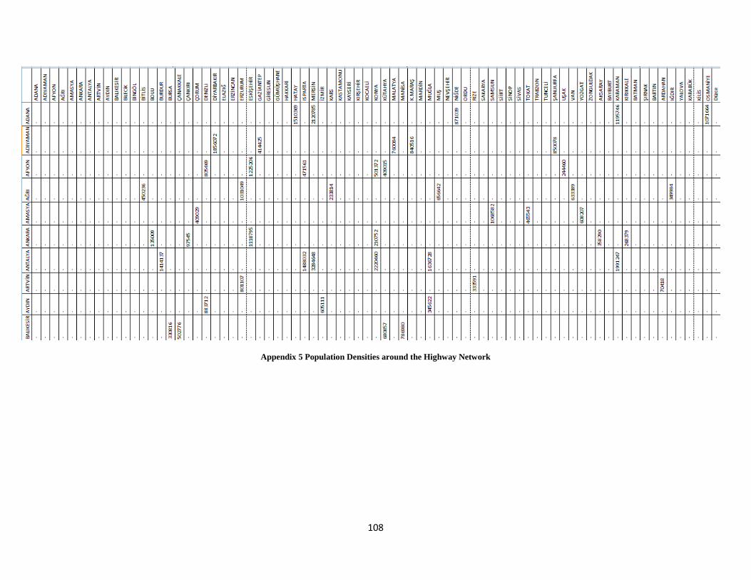
108
Appendix 5 Population Densities around the Highway Network
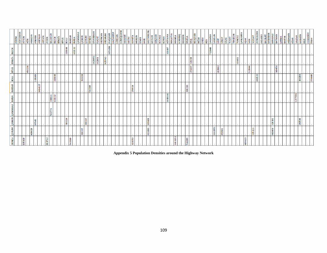
109
Appendix 5 Population Densities around the Highway Network
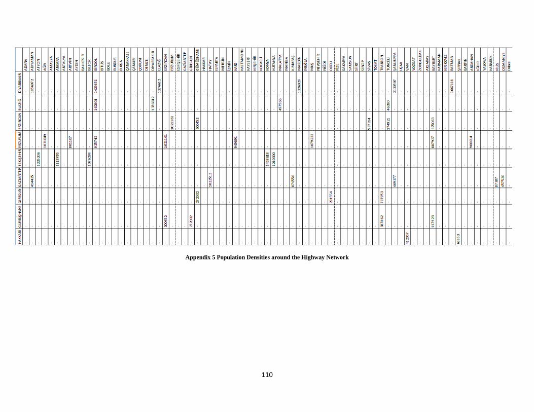
110
Appendix 5 Population Densities around the Highway Network
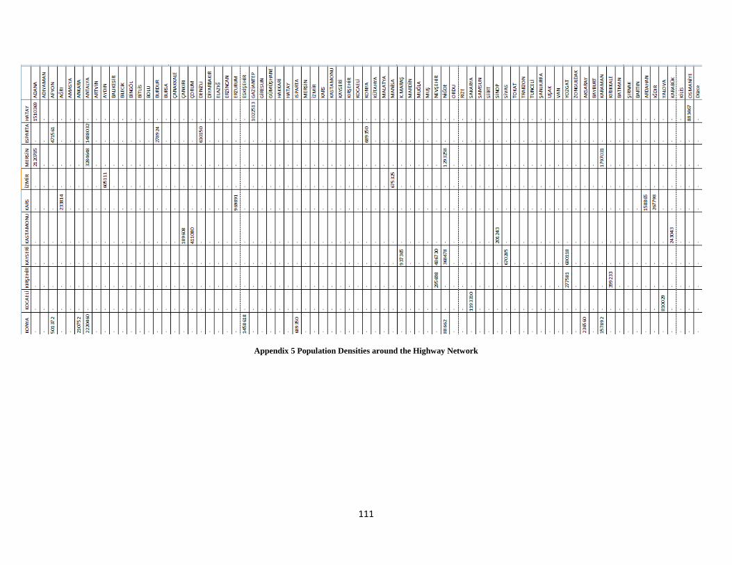
111
Appendix 5 Population Densities around the Highway Network
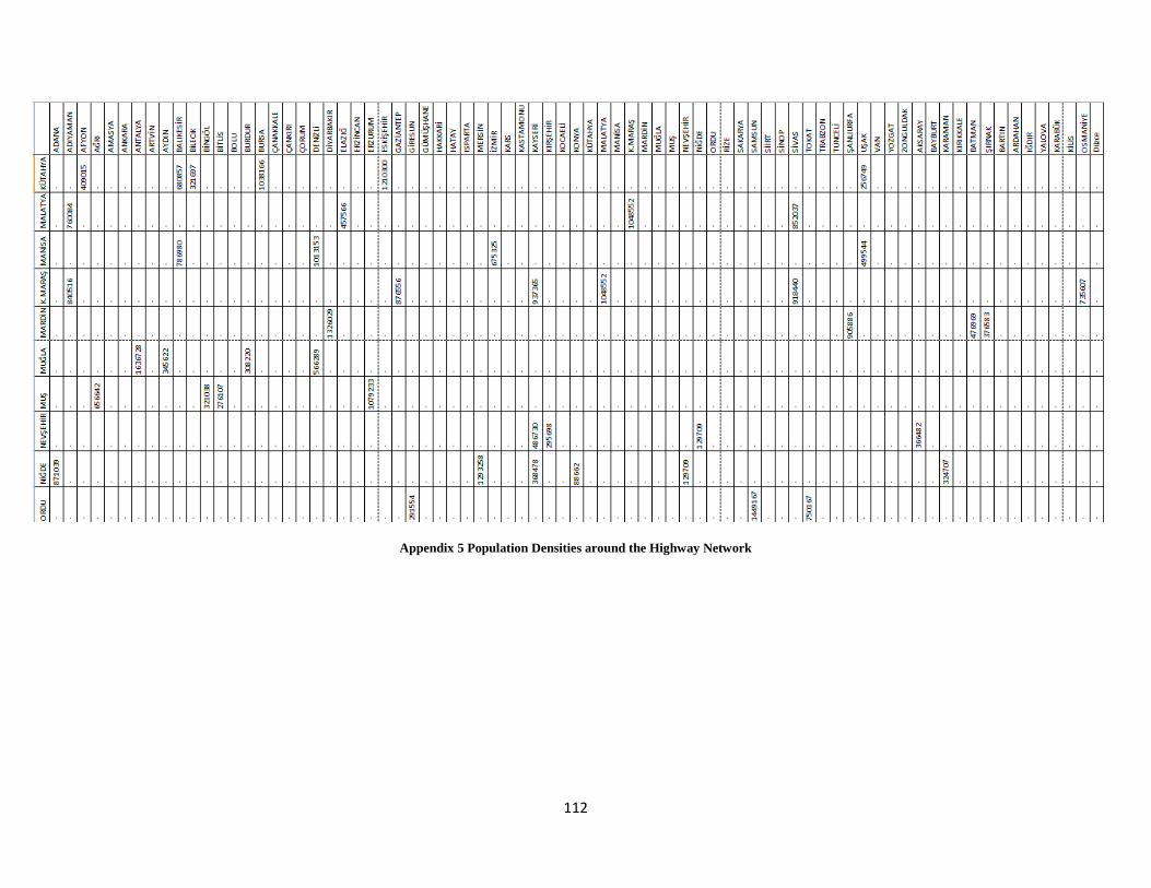
112
Appendix 5 Population Densities around the Highway Network
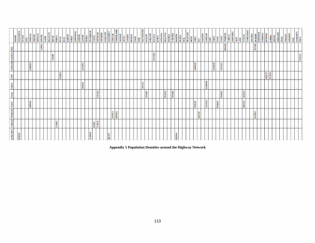
113
Appendix 5 Population Densities around the Highway Network
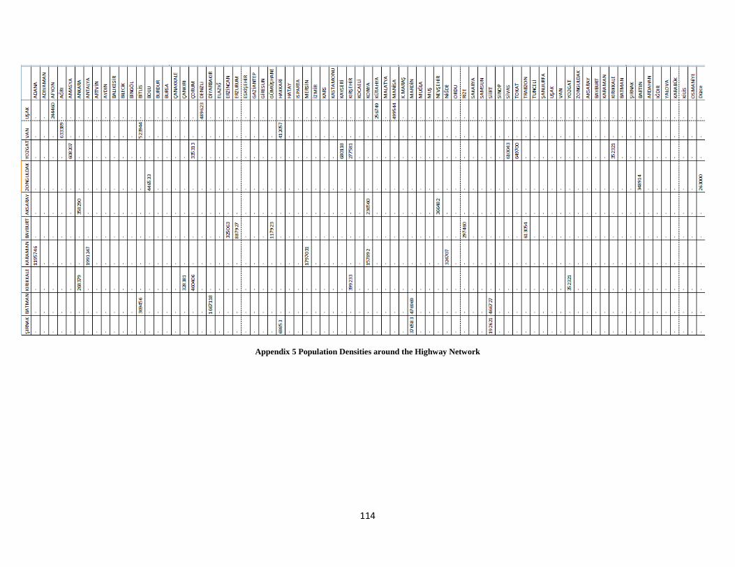
114
Appendix 5 Population Densities around the Highway Network
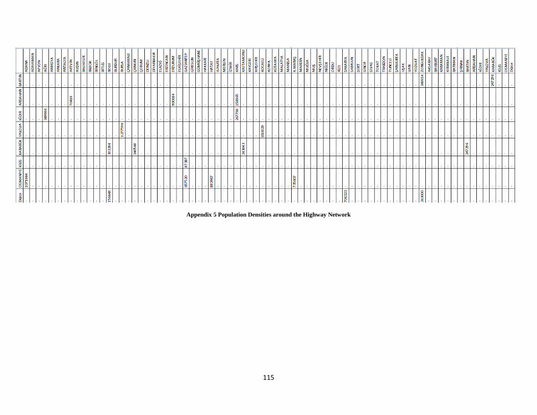
115
Appendix 5 Population Densities around the Highway Network
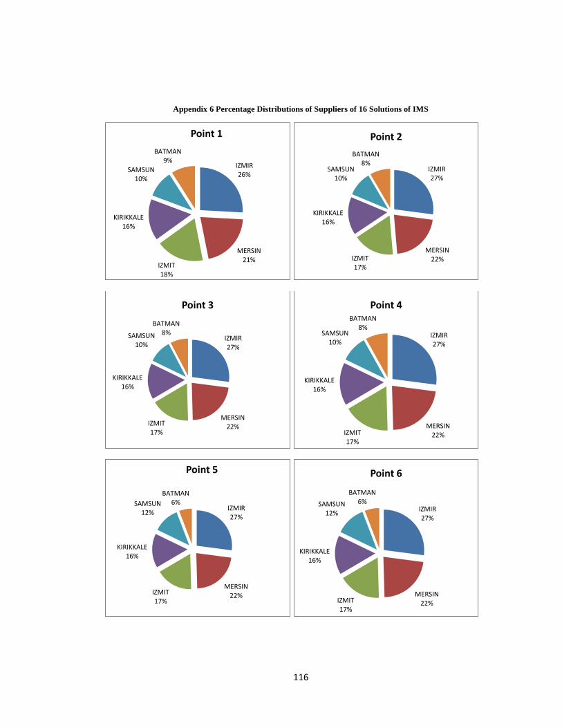
116
Appendix 6 Percentage Distributions of Suppliers of 16 Solutions of IMS
IZMIR 26%
MERSIN 21%
IZMIT 18%
KIRIKKALE 16%
SAMSUN 10%
BATMAN 9%
Point 1
IZMIR 27%
MERSIN 22% IZMIT
17%
KIRIKKALE 16%
SAMSUN 10%
BATMAN 8%
Point 2
IZMIR 27%
MERSIN 22% IZMIT
17%
KIRIKKALE 16%
SAMSUN 10%
BATMAN 8%
Point 3
IZMIR 27%
MERSIN 22% IZMIT
17%
KIRIKKALE 16%
SAMSUN 10%
BATMAN 8%
Point 4
IZMIR 27%
MERSIN 22% IZMIT
17%
KIRIKKALE 16%
SAMSUN 12%
BATMAN 6%
Point 5
IZMIR 27%
MERSIN 22% IZMIT
17%
KIRIKKALE 16%
SAMSUN 12%
BATMAN 6%
Point 6

117
IZMIR 27%
MERSIN 25%
IZMIT 17%
KIRIKKALE 14%
SAMSUN 12%
BATMAN 5%
Point 7
IZMIR 27%
MERSIN 25%
IZMIT 16%
KIRIKKALE 15%
SAMSUN 12%
BATMAN 5%
Point 8
IZMIR 27%
MERSIN 31%
IZMIT 13%
KIRIKKALE 18%
SAMSUN 6%
BATMAN 5%
Point 9
IZMIR 28%
MERSIN 35%
IZMIT 9%
KIRIKKALE 20%
SAMSUN 5%
BATMAN 3%
Point 10
IZMIR 27%
MERSIN 40%
IZMIT 6%
KIRIKKALE 19%
SAMSUN 5%
BATMAN 3%
Point 11
IZMIR 23%
MERSIN 44%
IZMIT 6%
KIRIKKALE 19%
SAMSUN 5%
BATMAN 3%
Point 12
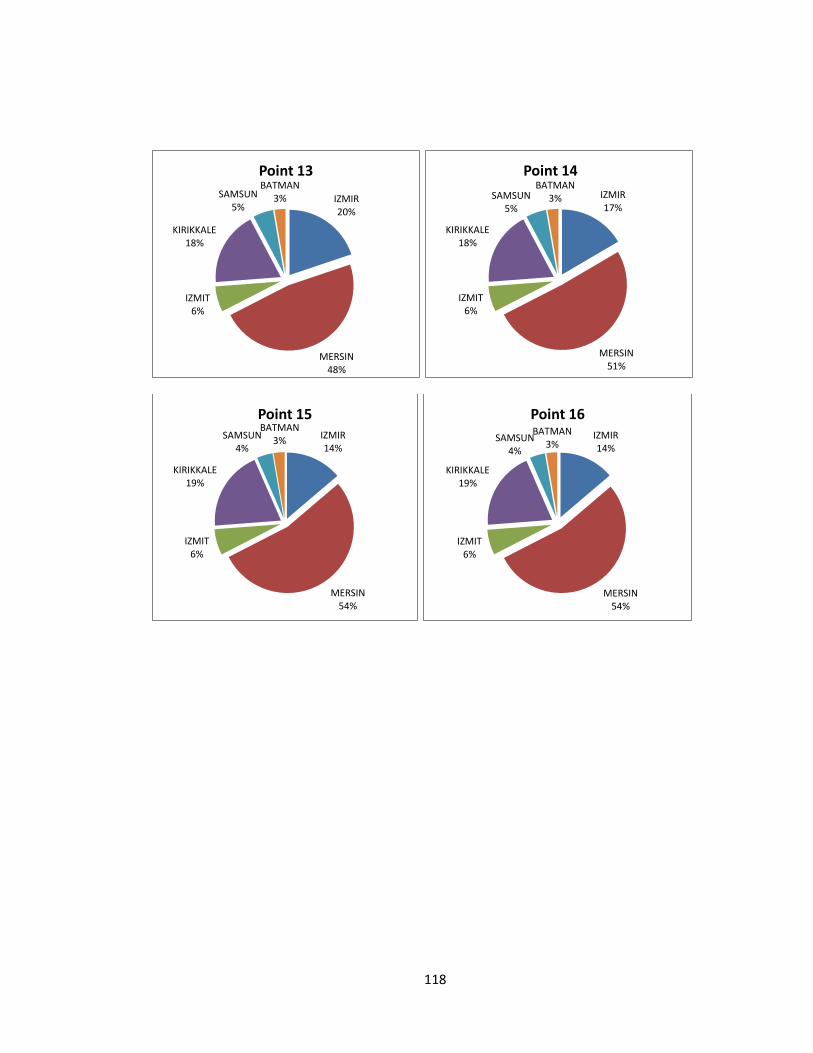
118
IZMIR 20%
MERSIN 48%
IZMIT 6%
KIRIKKALE 18%
SAMSUN 5%
BATMAN 3%
Point 13
IZMIR 17%
MERSIN 51%
IZMIT 6%
KIRIKKALE 18%
SAMSUN 5%
BATMAN 3%
Point 14
IZMIR 14%
MERSIN 54%
IZMIT 6%
KIRIKKALE 19%
SAMSUN 4%
BATMAN 3%
Point 15 IZMIR 14%
MERSIN 54%
IZMIT 6%
KIRIKKALE 19%
SAMSUN 4%
BATMAN 3%
Point 16
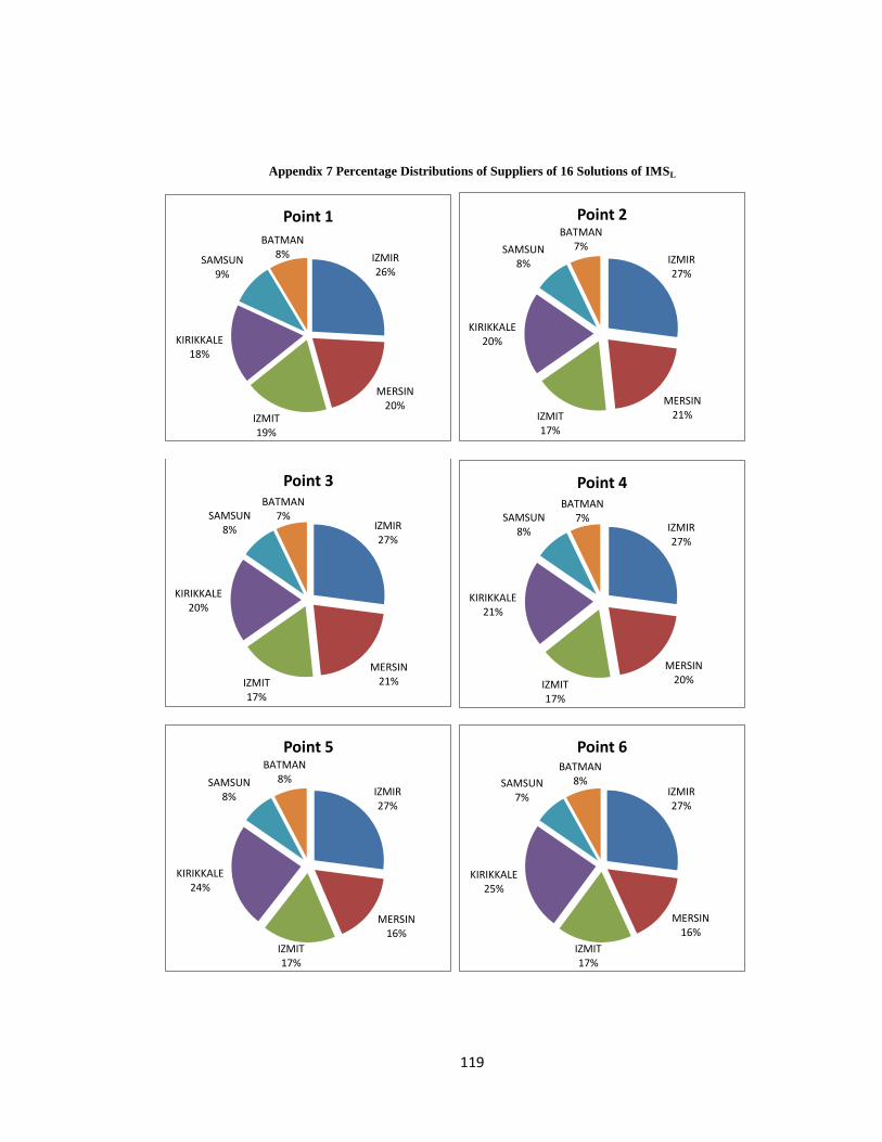
119
Appendix 7 Percentage Distributions of Suppliers of 16 Solutions of IMSL
IZMIR 26%
MERSIN 20%
IZMIT 19%
KIRIKKALE 18%
SAMSUN 9%
BATMAN 8%
Point 1
IZMIR 27%
MERSIN 21% IZMIT
17%
KIRIKKALE 20%
SAMSUN 8%
BATMAN 7%
Point 2
IZMIR 27%
MERSIN 21% IZMIT
17%
KIRIKKALE 20%
SAMSUN 8%
BATMAN 7%
Point 3
IZMIR 27%
MERSIN 20% IZMIT
17%
KIRIKKALE 21%
SAMSUN 8%
BATMAN 7%
Point 4
IZMIR 27%
MERSIN 16%
IZMIT 17%
KIRIKKALE 24%
SAMSUN 8%
BATMAN 8%
Point 5
IZMIR 27%
MERSIN 16%
IZMIT 17%
KIRIKKALE 25%
SAMSUN 7%
BATMAN 8%
Point 6
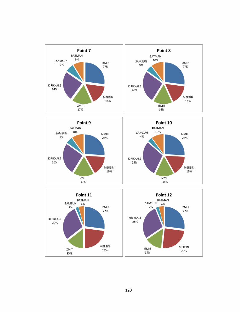
120
IZMIR 27%
MERSIN 16%
IZMIT 17%
KIRIKKALE 24%
SAMSUN 7%
BATMAN 9%
Point 7
IZMIR 27%
MERSIN 16%
IZMIT 16%
KIRIKKALE 26%
SAMSUN 5%
BATMAN 10%
Point 8
IZMIR 26%
MERSIN 16%
IZMIT 17%
KIRIKKALE 26%
SAMSUN 5%
BATMAN 10%
Point 9
IZMIR 26%
MERSIN 16%
IZMIT 15%
KIRIKKALE 29%
SAMSUN 4%
BATMAN 10%
Point 10
IZMIR 27%
MERSIN 23% IZMIT
15%
KIRIKKALE 29%
SAMSUN 2%
BATMAN 4%
Point 11
IZMIR 27%
MERSIN 25%
IZMIT 14%
KIRIKKALE 28%
SAMSUN 2%
BATMAN 4%
Point 12

121
IZMIR 27%
MERSIN 25% IZMIT
12%
KIRIKKALE 30%
SAMSUN 2%
BATMAN 4%
Point 13
IZMIR 25%
MERSIN 27% IZMIT
11%
KIRIKKALE 31%
SAMSUN 2%
BATMAN 4%
Point 14
IZMIR 21%
MERSIN 31%
IZMIT 11%
KIRIKKALE 31%
SAMSUN 2%
BATMAN 4%
Point 15
IZMIR 18%
MERSIN 34%
IZMIT 11%
KIRIKKALE 31%
SAMSUN 2%
BATMAN 4%
Point 16


