i
Indoor Cooperative Localization for Ultra
Wideband Wireless Sensor Networks
A Dissertation
Submitted to the Faculty
of the
WORCESTER POLYTECHNIC INSTITUTE
in partial fulfillment of the requirements for the
Degree of Doctor of Philosophy
in
Electrical and Computer Engineering
by
__________________________________
Nayef Alsindi
April 2008
APPROVED
____________________
Prof. Kaveh Pahlavan, Advisor
________________________
Prof. Fred J. Looft, Head, ECE Department

ii
To My Wife
i
Abstract
In recent years there has been growing interest in ad-hoc and wireless sensor networks
(WSNs) for a variety of indoor applications. Localization information in these networks
is an enabling technology and in some applications it is the main sought after parameter.
The cooperative localization performance of WSNs is ultimately constrained by the
behavior of the utilized ranging technology in dense cluttered indoor environments.
Recently, ultra-wideband (UWB) Time-of-Arrival (TOA) based ranging has exhibited
potential due to its large bandwidth and high time resolution. However, the performance
of its ranging and cooperative localization capabilities in dense indoor multipath
environments needs to be further investigated. Of main concern is the high probability of
non-line of sight (NLOS) and Direct Path (DP) blockage between sensor nodes, which
biases the TOA estimation and degrades the localization performance.
In this dissertation, we first present the results of measurement and modeling of UWB
TOA-based ranging in different indoor multipath environments. We provide detailed
characterization of the spatial behavior of ranging, where we focus on the statistics of the
ranging error in the presence and absence of the DP and evaluate the pathloss behavior in
the former case which is important for indoor geolocation coverage characterization.
Parameters of the ranging error probability distributions and pathloss models are
provided for different environments: traditional office, modern office, residential and
manufacturing floor; and different ranging scenarios: indoor-to-indoor (ITI), outdoor-to-
indoor (OTI) and roof-to-indoor (RTI).

ii
Based on the developed empirical models of UWB TOA-based OTI and ITI ranging, we
derive and analyze cooperative localization bounds for WSNs in the different indoor
multipath environments. First, we highlight the need for cooperative localization in
indoor applications. Then we provide comprehensive analysis of the factors affecting
localization accuracy such as network and ranging model parameters.
Finally we introduce a novel distributed cooperative localization algorithm for indoor
WSNs. The Cooperative LOcalization with Quality of estimation (CLOQ) algorithm
integrates and disseminates the quality of the TOA ranging and position information in
order to improve the localization performance for the entire WSN. The algorithm has the
ability to reduce the effects of the cluttered indoor environments by identifying and
mitigating the associated ranging errors. In addition the information regarding the
integrity of the position estimate is further incorporated in the iterative distributed
localization process which further reduces error escalation in the network. The simulation
results of CLOQ algorithm are then compared against the derived G-CRLB, which shows
substantial improvements in the localization performance.
iii
Acknowledgements
I am extremely grateful to Professor Kaveh Pahlavan for his support and guidance
throughout my graduate studies. What I have learned from him was truly beyond
academics and research for he has spurred the growth of my professional career. I have
learned from his experiences and stories that carry many lessons in dealing with life’s
choices and struggles. I am sure that I will always revisit them to seek inspiration.
I would like to thank my dissertation committee members, Professor John Orr,
Professor Allen Levesque, Professor Alexander Wyglinski and Professor Xinrong Li for
their valuable suggestions, comments and encouragements.
My graduate experience at WPI was simply remarkable and for that I have to thank
and acknowledge my best friends who shared with me all my setbacks and successes
throughout the last 6 years. They are Engin Ayturk, Mohammad Heidari, Hamid
Ghadyani, Bardia Alavi, Erdinc Ozturk, and Ferit Akgul.
Finally, my accomplishments were only possible because of my wife’s continuous
support, encouragement and motivation. Dr. Abeer Al-naqbi has provided me with the
strength to persevere and succeed in the face of many adversities. I am also indebted to
my father, Dr. Ali Alsindi and mother Mrs. Manar Fakhri for their support and
investment in my upbringing and education. Also I would like to thank my brother and
sisters who are also my best friends: Dr. Fahad Alsindi, Noora Alsindi and Muneera
Alsindi.
iv
Table of Contents
Abstract .......................................................................................................................... i
Acknowledgements .......................................................................................................... iii
Table of Contents ............................................................................................................. iv
List of Figures.................................................................................................................. vii
List of Tables .................................................................................................................... xi
Chapter 1 Introduction................................................................................................... 1
1.1. Localization in Wireless Sensor Networks ......................................................... 1
1.2. Background and Motivation ............................................................................... 3
1.3. Contributions of the Dissertation ........................................................................ 8
1.4. Outline of the Dissertation .................................................................................. 9
Chapter 2 Node Localization in Indoor Environments: Concepts and Challenges 11
2.1. Evolution of Localization Techniques .............................................................. 11
2.2. Localization Systems ........................................................................................ 13
2.3. Popular Ranging Techniques ............................................................................ 16
2.3.1. TOA-based Ranging ................................................................................. 16
2.3.2. RSS-based Ranging .................................................................................. 20
2.4. Wireless Localization Algorithms .................................................................... 21
2.4.1. Background ............................................................................................... 21
2.4.2. Least Squares (LS) Algorithm .................................................................. 23
2.4.3. Weighted Least Squares (WLS) Algorithms ............................................ 26
2.5. Practical Performance Considerations .............................................................. 26
2.6. Cooperative Localization in WSNs .................................................................. 28
2.6.1. Background ............................................................................................... 28
2.6.2. Cooperative Localization Techniques....................................................... 31
2.6.3. Challenges Facing Distributed Localization Algorithms.......................... 32
Chapter 3 UWB TOA-based Ranging: Concepts, Measurements & Modeling ...... 35
3.1. Background ....................................................................................................... 35
3.2. UWB TOA-based Ranging Concepts ............................................................... 38

v
3.2.1. Ranging Coverage..................................................................................... 40
3.2.2. Ranging Error............................................................................................ 42
3.2.3. Factors Affecting Ranging Coverage and Accuracy ................................ 44
3.3. UWB Measurement Campaign ......................................................................... 45
3.3.1. Background ............................................................................................... 45
3.3.2. Measurement System................................................................................ 45
3.3.3. Measurement Locations and Procedure .................................................... 46
3.3.4. Post-Processing ......................................................................................... 49
3.4. Modeling the Pathloss....................................................................................... 50
3.5. Modeling the Ranging Error ............................................................................. 55
3.5.1. Spatial Characterization ............................................................................ 55
3.5.2. Probability of DP Blockage ...................................................................... 56
3.5.3. Behavior in the Presence of DP ................................................................ 58
3.5.4. Behavior in the Absence of DP................................................................. 61
3.6. Simulation Results ............................................................................................ 67
3.6.1. Predicting Ranging Coverage ................................................................... 67
3.6.2. Ranging Error Simulation ......................................................................... 69
3.7. Conclusion ........................................................................................................ 73
Chapter 4 Cooperative Localization Bounds for Indoor UWB WSNs..................... 75
4.1. Introduction....................................................................................................... 75
4.2. UWB TOA-based Ranging Overview .............................................................. 79
4.3. Problem Formulation ........................................................................................ 81
4.4. The Generalized Cramer-Rao Lower Bound .................................................... 83
4.5. Simulation Results ............................................................................................ 88
4.5.1. Setup ......................................................................................................... 88
4.5.2. Traditional VS Cooperative Localization ................................................. 90
4.5.3. Network Parameters.................................................................................. 92
4.5.4. Ranging Model Parameters....................................................................... 95
4.6. Conclusion ........................................................................................................ 99
Chapter 5 A Cooperative Localization Algorithm for Indoor WSNs .................... 102
5.1. Background ..................................................................................................... 102
vi
5.2. Cooperative LOcalization with Quality of estimation (CLOQ) ..................... 106
5.2.1. Overview................................................................................................. 106
5.2.2. Step I: Channel Identification ................................................................. 109
5.2.3. Step II: Position Estimation .................................................................... 118
5.2.4. Step III: Anchor Nomination .................................................................. 123
5.2.5. Step IV: New Anchor Incorporation....................................................... 125
5.3. Performance Analysis ..................................................................................... 127
5.3.1. Simulation Setup..................................................................................... 127
5.3.2. Node Density .......................................................................................... 128
5.3.3. Anchor Density ....................................................................................... 129
Chapter 6 Conclusion & Future Work ..................................................................... 133
6.1. Conclusion ...................................................................................................... 133
6.2. Future Work .................................................................................................... 135
References ..................................................................................................................... 137
vii
List of Figures
Figure 2.1: Localization block diagram. ........................................................................ 14
Figure 2.2: Localization with 3 anchors. ........................................................................ 15
Figure 2.3: TOA ranging between sensors. The TOA can be measured by recording the
time it takes to transmit and receive a packet between two nodes. If
however, the direct path signal is block then the time delay or distance
estimation is biased which can cause significant errors in the localization
process.......................................................................................................... 17
Figure 2.4: TOA estimation in the presence of DP. The accuracy of TOA estimation
depends on the availability of the DP signal. In this case, the DP signal
power is well above the detection threshold and thus can provide accurate
distance estimation....................................................................................... 18
Figure 2.5: TOA estimation in the absence of the DP. In this condition, the DP signal
power is attenuated and cannot be detected. As a result the first arriving path
is used for TOA ranging instead causing significant estimation errors. ...... 19
Figure 2.6: Ranging using RSS is implemented by estimating the distance from the
signal power. A sensor node measures the received power from another
node and translates that into an estimated distance. The distance estimates
using this technique lack accuracy due to the method’s reliance on pathloss
models and the indirect relationship between power and distance. ............. 20
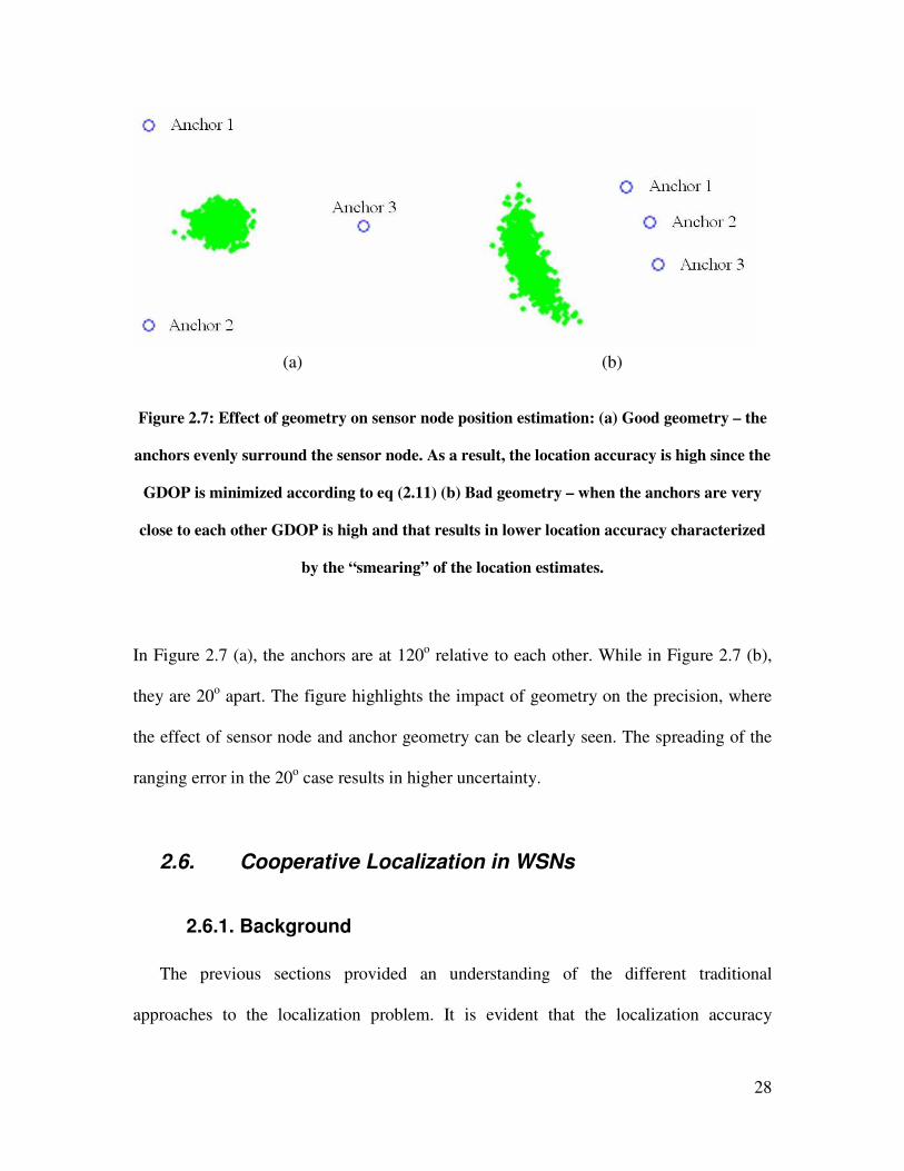
Figure 2.7: Effect of geometry on sensor node position estimation: (a) Good geometry –
the anchors evenly surround the sensor node. As a result, the location
accuracy is high since the GDOP is minimized according to eq (2.11) (b)
Bad geometry – when the anchors are very close to each other GDOP is
high and that results in lower location accuracy characterized by the
“smearing” of the location estimates. .......................................................... 28
viii
Figure 2.8: Cooperative localization concept in WSN. (a) Traditional wireless networks.
(b) WSNs. Black circles are anchor nodes and white circles are “blind”
sensor nodes. In WSNs the cooperation between the sensor nodes allows for
increased information sharing. This specifically provides enhanced coverage
and improvement in localization accuracy. ................................................. 30
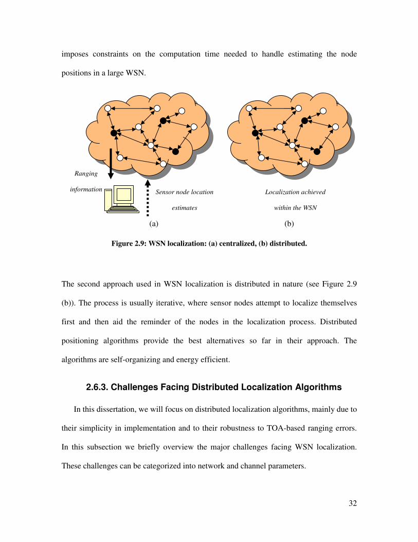
Figure 2.9: WSN localization: (a) centralized, (b) distributed. ...................................... 32
Figure 3.1: Indoor Ranging Scenarios. In many of the potential indoor geolocation
applications sensor nodes will be deployed inside, outside and on top of
buildings. As a result understanding the impact of those scenarios on TOA-
based ranging is very important for accurate and reliable localization. ...... 36
Figure 3.2: UWB frequency domain measurement system............................................ 46
Figure 3.3: Sample measurement floor plans. (a) Fuller OTI/ITI (b) Schussler OTI/ITI
(c) Norton ITI (d) AK RTI. Squares are Tx locations and dots are Rx
locations ....................................................................................................... 48
Figure 3.4: Pathloss scatter plots in Fuller ITI at 3 GHz bandwidth.............................. 51
Figure 3.5: Pathloss scatter plots in Norton OTI at 500 MHz bandwidth...................... 52
Figure 3.6: Pathloss scatter plots in AK RTI at 500 MHz.............................................. 52
Figure 3.7: Norton ITI at 500 MHz bandwidth: confirming the normality of the biases in
LOS conditions ............................................................................................ 59
Figure 3.8: Schussler ITI NLOS: mean of biases is larger than LOS ............................ 60
Figure 3.9: Schussler OTI at 3 GHz bandwidth: confirming the lognormality of the
measured normalized ranging error ............................................................. 64
Figure 3.10: Fuller OTI at 500 MHz bandwidth: confirming the lognormality of the
measured normalized ranging error ............................................................. 65
Figure 3.11: AK RTI at 3 GHz bandwidth: confirming the lognormality of the measured
normalized ranging error.............................................................................. 65
ix
Figure 3.12: Simulating ranging coverage for system bandwidths (a) 500 MHz (b) 3
GHz. The increase in bandwidth decreases ranging coverage due to lower
energy per MPC. .......................................................................................... 68
Figure 3.13: CDF of normalized ranging error: simulation vs. measurements. (a)
Schussler OTI (b) AK RTI........................................................................... 71
Figure 3.14: CDF of normalized ranging error: simulation vs. measurements. (a) Norton
OTI (b) Fuller OTI ....................................................................................... 72
Figure 4.1: Indoor cooperative localization application. Squares are anchor nodes and
circles are sensor nodes. Connectivity based on Fuller models at 500 MHz.
...................................................................................................................... 76
Figure 4.2: OTI/ITI ranging coverage and the associated ranging error conditions. I:
λ (LOS), II: η (NLOS – DP), III: β (NLOS – NDP). ................................ 80
Figure 4.3: Percentage of un-localized sensor nodes as a function of OTI
cD R . ............. 91
Figure 4.4: Traditional triangulation vs. cooperative localization performance. ........... 92
Figure 4.5: Localization performance as a function of node density in different indoor
environments using 500 MHz models. ........................................................ 93
Figure 4.6: Localization performance as a function of number of anchors in different
indoor environments using 500 MHz models. ............................................. 94
Figure 4.7: Localization Performance as a function of dynamic range, ρ for 500 MHz
and 3 GHz models........................................................................................ 96
Figure 4.8: Localization performance as a function of ( )1p G = for 500 MHz and 3 GHz
models. ......................................................................................................... 97
Figure 4.9: Localization performance as a function of DP blockage probability,
( )1p X = for 500 MHz and 3 GHz models................................................. 98
Figure 5.1: Direct Ranging - Recursive Position Estimation Distributed Localization103
Figure 5.2: Extended Ranging - Multi-hop Distributed Localization .......................... 104
x
Figure 5.3: Quality of range measurements & position estimates. (a) Bad geometry but
acceptable range measurements. (b) Good geometry but unreliable
measurements............................................................................................. 107
Figure 5.4: Database classification for channel identification ..................................... 110
Figure 5.5: Probability plots of ITI data and their distribution fits at (a) 500 MHz and
(b) 3 GHz. .................................................................................................. 111
Figure 5.6: Distribution fits and the respective thresholds. (a) 500 MHz and (b) 3 GHz.
.................................................................................................................... 113
Figure 5.7: Probability plots of OTI data and their distribution fits at (a) 500 MHz and
(b) 3 GHz. .................................................................................................. 115
Figure 5.8: Distribution fits and the respective thresholds. (a) 500 MHz and (b) 3 GHz.
.................................................................................................................... 117
Figure 5.9: CLOQ Algorithm – Stage II position estimation. Black circles are anchors,
grey circles are newly transformed anchors and white circles are un-
localized sensor nodes................................................................................ 121
Figure 5.10: CLOQ Algorithm – Stage III Anchor Nomination. Black circles are anchor
nodes, grey circles are anchor nominees and white circles are un-localized
sensor nodes. .............................................................................................. 124
Figure 5.11: CLOQ Algorithm flow diagram................................................................. 126
Figure 5.12: Localization Performance in Fuller Building at 3 GHz. ............................ 129
Figure 5.13: Localization Performance as a function of number of anchors. ................ 130
Figure 5.14: CLOQ – % of un-localized nodes as a function of building dimension. ... 131
xi
List of Tables
Table 3.1: Summary of the measurement database....................................................... 47
Table 3.2: Pathloss parameters...................................................................................... 53
Table 3.3 Probabilities of the presence and absence of the DP ................................... 57
Table 3.4: DP normal distribution modeling parameters for normalized ranging error 61
Table 3.5: Passing rate of K-S hypothesis test at 5% significance level ...................... 62
Table 3.6: Lognormal distribution modeling parameters of the normalized ranging
error in the absence of the direct path.......................................................... 66
Table 5.1: Distribution parameters for δ . .................................................................. 118
Table 5.2: ITI and OTI decision thresholds ................................................................ 118
Table 5.3: Connectivity information that node 6 gathers about surrounding anchors.122
1
Chapter 1 Introduction
1.1. Localization in Wireless Sensor Networks
In recent years there has been growing interest in ad-hoc and wireless sensor networks
(WSNs) for a variety of applications. The development of microelectromechanical
systems (MEMS) technology as well as the advancement in digital electronics and
wireless communications has made it possible to design small size, low-cost energy
efficient sensor nodes that could be deployed in different environments for a variety of
applications [Aky02]. Node localization is an enabling technology for WSNs because
sensor nodes deployed in an area of interest usually need position information for routing
and application-specific tasks, such as temperature and pressure monitoring [Pat05]. In
many applications, a WSN is deployed to help improve localization accuracy in
environments where the channel condition poses a challenge to range estimation [Pah06].
In such environments, cooperative localization provides a potential for many applications
in the commercial, public safety and military sectors [Pah06, Pah02]. In commercial
applications, there is a need for localizing and tracking inventory items in warehouses,
materials and equipment in manufacturing floors, elderly in nursing homes, medical
equipment in hospitals, and objects in residential homes. In public safety and military
applications, however, indoor localization systems are needed to track inmates in prisons
and navigate policemen, fire fighters and soldiers to complete their missions inside
buildings [Pah02]. Node localization plays an important role in all these WSN
applications.
2
In certain vital indoor cooperative localization applications, such as fire-fighting and
military operations, a small number of sensors called anchors are deployed outside
surrounding a building where they obtain their location information via GPS or are pre-
programmed during setup. The un-localized sensor nodes are then deployed inside the
building, e.g. carried by firefighters or soldiers entering a hostile building, who with the
help of the anchors attempt to obtain their own location information. In traditional
approaches, such as trilateration (triangulation) techniques, the exterior anchor nodes
usually fail to cover a large building, which makes localization ineffective. In addition,
the problems of indoor multipath and non-line-of-sight (NLOS) channel conditions
further degrade the range estimates, yielding unreliable localization performance [Pah02].
Implementation of the cooperative localization approach extends the coverage of the
outside anchors to the inside nodes and has the ability to enhance localization accuracy
through the availability of more range measurements between the sensor nodes.
Effective cooperative localization in indoor WSNs does however hinge on the ranging
technology. Among the emerging techniques, Ultra Wideband (UWB) Time of Arrival
(TOA)-based ranging has recently received considerable attention [Gez05, Gha04,
Opp04]. In addition to its high data rate communications, it has been selected as a viable
candidate for precise ranging and localization. This is mainly due to its large system
bandwidth which offers high resolution and signaling that allows for centimeter
accuracies, low-power and low-cost implementation [Por03, Gez05]. The performance of
this technique, nevertheless, depends on the availability of the direct path (DP) signal
between a pair of sensor nodes [Lee02, Pah98]. In the presence of the DP, i.e. short
distance line-of-sight (LOS) conditions, accurate UWB TOA estimates in the range of
3
centimeters are feasible due to the high time-domain resolution [Fon02, Chu03, Ala06,
Tar06]. However, the challenge is UWB ranging in indoor NLOS conditions, which can
be characterized as dense multipath environments [Lee02, Pah98]. In these conditions
the DP between a pair of nodes can be blocked with high probability, substantially
degrading the range and localization accuracy. Therefore, there is a need to analyze the
impact of these channel limitations on the performance of cooperative localization in
indoor WSNs.
This dissertation is concerned with the evaluation of cooperative localization in indoor
WSNs from the radio propagation channel perspective. We intend to provide detailed
analysis on the impact of the indoor multipath and NLOS conditions on the UWB TOA-
based ranging and cooperative localization in WSNs. Next we provide detailed
description of the motivation and contributions of the dissertation.
1.2. Background and Motivation
Indoor localization is one of the newly emerging technologies having potential for
numerous applications in the commercial and public safety fields. The enabling of robust
and accurate localization in harsh indoor environment faces real physical challenges,
especially for TOA-based systems where the probability of NLOS and blockage of the
DP between mobile nodes is very high [Pah98, Pah02]. The main challenges in these
environments are multipath, NLOS propagation, DP blockage and insufficient signal
coverage. Several techniques have been proposed to combat multipath for low bandwidth
systems [Dum94, Li04]. These techniques have the potential to increase the time-domain
resolution of the received waveform, mitigate multipath in indoor environments and
4
improve TOA ranging accuracy. Recently, UWB signals have showed promising
potential for accurate TOA-based ranging and localization due to the available excess
system bandwidth [Fon02, Lee02, Mol05]. However, these algorithms and techniques
still suffer in harsh NLOS propagation and DP blockage environments where the
degradation of the DP signal causes substantial ranging errors [Pah06]. Fortunately, the
majority of the current research thrust in NLOS localization has been towards NLOS or
DP blockage identification and mitigation [Che99, Wei05, Gev07, Hei07, Ven07a,
Ven07b, Als08c]. The localization performance using these techniques have showed
promising potential, where the channel statistics and signal information are incorporated
in a decision theoretic framework to mitigate “bad” estimates before incorporation into
localization algorithms.
Although these algorithms and techniques can improve the localization performance,
they still face further physical limitations specific to the indoor environment. In outdoor
GPS applications the accuracy is directly related to the Geometric Dilution of Precision
(GDOP) where the number of satellites in view and their locations relative to the mobile
user can have significant impact on the performance [Kap96]. Similarly, in indoor
environments a large number of Reference Points (RPs) or anchors are needed in order to
achieve acceptable levels of accuracy [Pah06]. For the majority of indoor applications the
limited radio coverage of RPs/anchors in large buildings implies that there exists a high
probability of insufficient coverage to enable effective localization [Pah06]. More
importantly for the outdoor-indoor applications such as the firefighting or military
operations the radio coverage is further diminished due to the signal having to penetrate
5
external building structures. This then poses questions as to the reliability and accuracy of
TOA-based localization systems under these constraints.
One promising alternative to these challenges in indoor environments is UWB TOA-
based cooperative localization using WSNs [Pah06, Gez05]. Unlike traditional
localization techniques, cooperative localization in WSNs allows for ranging information
to be exchanged between nodes and anchors as well as nodes and other nodes in the
network. Coupled with UWB TOA-based ranging, cooperative localization has the
potential to remedy many of the problems and challenges plaguing indoor localization
applications. The UWB signals will allow for high resolution and thus very accurate
ranging capability. In addition, cooperative localization will provide the ability to combat
the NLOS/DP-blockage and limited coverage problems due to the redundancy in TOA-
range information connecting the network.
In 2005, the Center for Wireless Information Network Studies (CWINS) at WPI with
Innovative Wireless Technologies (IWT) were awarded a research fund sponsored by
DARPA/DoD SBIR: BAA 03-029 entitled: “Innovative Methods for Geolocation and
Communication with Ultra Wideband Mobile Radio Networks”. The project spanned
different aspects of UWB localization. IWT were responsible for the design and
implementation of the UWB radios while CWINS took charge of characterizing the
empirical behavior of TOA-based ranging using UWB. As a result the foundation of this
dissertation is the UWB measurement campaign that was conducted in the summer of
2005. The measurements provided a platform for evaluating the behavior of the UWB
TOA-based ranging in different indoor environments.
6
In order to asses the potential of UWB cooperative localization in indoor
environments, however, it is important to develop an analytical framework that addresses
the different layers of the problem. At the ranging layer, understanding the behavior of
UWB TOA-based ranging in indoor environments is essential. This can be accomplished
by conducting UWB measurements and modeling of the TOA-based ranging. Several
indoor propagation experiments with a focus on indoor ranging, be it UWB or otherwise,
have been reported in the literature [Fon02, Lee02, Pah98, Ala03a, Tar06, Den04, Fal06,
Ala06, Pat03, Hat06, Ala05, Low05]. These experiments have usually been limited to a
floor or several rooms but do not address modeling the spatial statistics of NLOS ranging
nor ranging coverage. The only available ranging error models were provided in [Den04,
Ala06] but are based on limited measurement data sets, and only the latter focuses on
characterization of errors according to the availability of the DP. As a result, a
comprehensive measurement and modeling of UWB TOA-based ranging in different
indoor environments and scenarios is needed but is not available in the literature.
At the localization layer, these ranging models should be used to evaluate the impact
of the radio propagation channel on cooperative localization in indoor WSNs. In turn this
could be achieved by integrating the empirical models in developing theoretical
performance bounds (e.g. CRLB-type bounds) and assessing the accuracy of cooperative
localization algorithms. In the literature, localization bounds in multi-hop WSNs have
been examined extensively [Lar04, Sav05, Cha06], where the focus has been on
analyzing the impact of network parameters such as the number of anchors, node density
and deployment topology affecting localization accuracy, etc. However, these
localization bounds have been analyzed with unbiased generic ranging assumptions
7
between sensor nodes. In [Koo98, Bot04] the impact of biased TOA range measurements
on the accuracy of location estimates is investigated for cellular network applications.
Their approach assumes NLOS induced errors as small perturbations, which clearly is not
the case in indoor environments. A comprehensive treatment of the impact of biases on
the traditional wireless geolocation accuracy in NLOS environments is reported in
[Qi06]. Recently, position error bounds for dense cluttered indoor environments have
been reported in [Jou06a, Jou06b] where the impact of the channel condition on the
localization error is further verified in traditional localization. As a result there is a need
for the derivation and analysis of the theoretical performance bounds for UWB
cooperative localization in indoor-specific WSNs.
Another important research direction in this emerging field is the development of
cooperative localization algorithms for WSNs. Unfortunately, most of the algorithms in
the literature are generic and they do not address the impact of the indoor propagation
channel on the ranging and localization performance [Savr01, Savr02, Alb01, Nic01].
Although those algorithms might yield unacceptable performance in indoor
environments, they provide practical ideas for localizing nodes in large sensor networks.
Therefore, there is a need for novel cooperative localization algorithms that are
specifically designed for the harsh indoor environment.
The principle goal of this research work is to develop an analytical framework for
assessing the impact of the indoor propagation channel on the performance of UWB
TOA-based cooperative localization in WSNs. Specifically we define three major
objectives of this research work. The first is to conduct large-scale measurements and
modeling of the UWB TOA-based ranging in indoor multipath environments. The second

8
is to incorporate these empirical measurements and models into an analytical framework
that can be used to assess the impact of indoor ranging on cooperative localization. The
third objective of this work is to develop a novel cooperative localization algorithm that
has the ability to improve localization accuracy by incorporating the channel statistics in
the estimation process. The algorithm takes advantage of the models and attempts to
quantify the quality of ranging and localization in order to improve the performance.
1.3. Contributions of the Dissertation
In this dissertation we first provide an overview of the basics of cooperative
localization and the challenges facing this emerging technology where the impact of the
channel on the localization performance is highlighted and the major cooperative
localization bounds and algorithms are discussed. This work is presented in Chapter 2
and has been published in [Als08d]. Then we present the research work which focuses on
three contributions to the field of WSN localization:
• Analysis, measurement and modeling of UWB TOA-based ranging in indoor
multipath environments. The work presents empirical results of the measurement
campaign in four different building environments: residential, traditional office,
modern office and a manufacturing floor; and three different ranging scenarios:
Indoor-to-Indoor (ITI), Outdoor-to-Indoor (OTI) and Roof-to-Indoor (RTI) using
two different UWB system bandwidths. These empirical measurements are used
to develop novel models that characterize TOA-based ranging coverage and error.
Specifically the former model provides a characterization for the feasible ranging
distance in indoor environments; while the latter provides statistical
9
characterization of ranging error in the different conditions such as LOS, NLOS
and DP blocked NLOS. This work is presented in Chapter 3 of the dissertation
and has been published in [Als07a, Als07b, Als08a].
• Analytical derivation and performance evaluation of the cooperative localization
in WSNs through the Generalized Cramer Rao Lower Bound (G-CRLB) in dense
cluttered indoor environments. Using the empirical TOA-based ranging models,
we provide a novel framework for analyzing the performance of cooperative
localization for WSNs in different indoor environments using two different
systems bandwidths, 500 MHz and 3 GHz. The work focuses on analyzing the
impact of node density, anchor density, building dimension and probability of
NLOS and probability of DP blockage on the cooperative localization
performance. This research work is presented in Chapter 4 and has been published
in [Als08b].
• Development of a novel cooperative localization algorithm for indoor WSNs. We
introduce Cooperative LOcalization with Quality of estimation (CLOQ) which is
a novel algorithm that integrates the quality of the range (channel information)
and node position (anchor confidence) in a weighted least square technique to
provide accurate location information. This work is presented in Chapter 5 and
has been published in [Als06a, Als06b].
1.4. Outline of the Dissertation
This dissertation focuses on node localization in UWB WSNs. First we will introduce
the fundamental concepts related to node localization, discuss the major challenges for
10
node localization in WSNs, and present the major node localization techniques proposed
for WSNs. In Chapter 3 we discuss the basics of UWB TOA-based ranging and their
application to ranging and localization. We then introduce a comprehensive measurement
campaign to evaluate the UWB TOA based ranging in four different indoor building
environments and three different ranging scenarios: ITI, OTI and RTI. Using these
measurements we develop and introduce novel models that characterize empirically the
behavior of ranging coverage and error in dense cluttered indoor environments. In
Chapter 4, we derive and evaluate the G-CRLB for UWB TOA-based cooperative
localization in indoor WSNs using the empirical models. We then analyze and compare
the localization performance in different indoor environments. In Chapter 5, we introduce
the novel cooperative localization algorithm (CLOQ) and evaluate its performance
against the G-CRLB. Finally we conclude the dissertation in Chapter 6, where we
provide the major conclusions and suggest future work.
11
Chapter 2 Node Localization in Indoor
Environments: Concepts and Challenges
In this chapter, we first introduce the evolution of localization technologies, and then
we describe the basics of localization in traditional network settings. Finally, we
introduce the main approaches to cooperative localization in WSNs and discuss the major
challenges affecting their performance.
2.1. Evolution of Localization Techniques
The problem of locating mobile radios originated with military operations during
World War II, where it was critical to locate soldiers in emergency situations. About
twenty years later, during the Vietnam conflict, the US Department of Defense launched
a series of Global Positioning System (GPS) satellites to support military operations in
combat areas. In 1990, the signals from GPS satellites were made accessible to the
private sector for commercial applications such as fleet management, navigation, and
emergency assistance. Today, GPS technology is widely available in the civilian market
for personal navigation applications. Despite its success, however, the accuracy of GPS
positioning is significantly impaired in urban and indoor areas, where received signals
can suffer from blockage and multipath effects.
In 1996, the Federal Communications Commission (FCC) introduced regulations
requiring wireless service providers to be able to locate mobile callers in emergency
situations with specified accuracy, namely 100 meters accuracy 67% of the time. Such
12
emergency service is called E-911 in the U.S. and E-112 in many other countries. In a
manner similar to the release of the ISM bands and subsequent emergence of the wireless
local area network (WLAN) industry, the FCC mandate for E-911 services quickly gave
rise to the development of the wireless geolocation industry. In time, technologies have
been developed to implement the E-911 mandate [Caf98, McG02] including GPS assisted
techniques, a variety of Time of Arrival (TOA), Angle of Arrival (AOA), and Received
Signal Strength (RSS) techniques. A variety of TOA, time differential (TDOA) or
extension of time differential (EOTD) techniques require special location-measurement
hardware integrated in the base stations and in some cases accurate synchronization
between the mobile terminals and base stations (for cellular applications). In contrast
with those approaches, RSS systems provide a lower-cost solution that can avoid
additional hardware installation but does require incorporating training functions into the
system.
In the late 1990s, at about the same time that E-911 technologies were emerging,
another initiative for accurate indoor geolocation began independently. It was motivated
by a variety of envisioned applications for indoor location-sensing in commercial, public
safety, and military settings [Pah02, Kos00, Pot00]. In commercial applications for
residences and nursing homes, there is an increasing need for indoor location-sensing
systems to track people with special needs, e.g., the elderly, as well as children who are
away from visual supervision. In public safety and military applications, indoor location
sensing systems are needed to track inmates in prisons and to guide policemen, fire-
fighters, and soldiers in accomplishing their missions inside buildings. More recently,
location sensing has found its applications in location-based handoffs in wireless
13
networks [Pah00], location-based ad-hoc network routing [Ko98, Jai01], and location-
based authentication and security [Sma00]. These and other applications have stimulated
interests in modeling the propagation environment to assess the accuracy of different
sensing techniques [Pah98, Kri99] as well as in developing novel technologies to
implement the systems [Fon02, Bah00a, Bah00b]. The implementation of the first
generation of indoor positioning products using a variety of technologies has been
reported in [Wer98, Roo02a, Roo02b].
The natural evolution of these ranging and localization technologies makes their
integration into WSN applications possible. Understanding the fundamental concepts and
challenges of these technologies in traditional localization is a necessary bridge to WSN
localization.
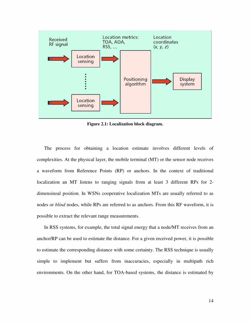
2.2. Localization Systems
In general, a localization system incorporates range measurements to determine the
location estimate. Figure 2.1 illustrates a block diagram of the main components in a
traditional localization system.
14
Figure 2.1: Localization block diagram.
The process for obtaining a location estimate involves different levels of
complexities. At the physical layer, the mobile terminal (MT) or the sensor node receives
a waveform from Reference Points (RP) or anchors. In the context of traditional
localization an MT listens to ranging signals from at least 3 different RPs for 2-
dimensinoal position. In WSNs cooperative localization MTs are usually referred to as
nodes or blind nodes, while RPs are referred to as anchors. From this RF waveform, it is
possible to extract the relevant range measurements.
In RSS systems, for example, the total signal energy that a node/MT receives from an
anchor/RP can be used to estimate the distance. For a given received power, it is possible
to estimate the corresponding distance with some certainty. The RSS technique is usually
simple to implement but suffers from inaccuracies, especially in multipath rich
environments. On the other hand, for TOA-based systems, the distance is estimated by
15
sending an RF signal and recording the time it takes to receive it. This approach is more
accurate because the arrival time corresponds to the direct path distance.
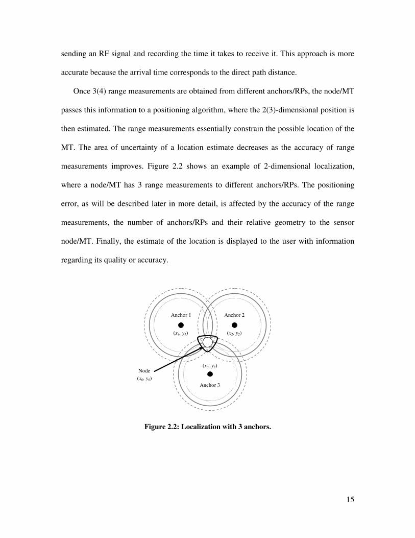
Once 3(4) range measurements are obtained from different anchors/RPs, the node/MT
passes this information to a positioning algorithm, where the 2(3)-dimensional position is
then estimated. The range measurements essentially constrain the possible location of the
MT. The area of uncertainty of a location estimate decreases as the accuracy of range
measurements improves. Figure 2.2 shows an example of 2-dimensional localization,
where a node/MT has 3 range measurements to different anchors/RPs. The positioning
error, as will be described later in more detail, is affected by the accuracy of the range
measurements, the number of anchors/RPs and their relative geometry to the sensor
node/MT. Finally, the estimate of the location is displayed to the user with information
regarding its quality or accuracy.
Anchor 1 Anchor 2
Anchor 3
Node
(x1, y1) (x2, y2)
(x3, y3)
(x0, y0)
Figure 2.2: Localization with 3 anchors.
16
WSN localization is a general case of the traditional localization but it is fundamentally
dependant on the building blocks in Figure 2.1. As a result, we will dedicate the first part
of this chapter to ranging and localization techniques in traditional network settings and
the second part to localization in WSNs. Understanding of ranging techniques and
localization algorithms is essential in building a fundamental basis for WSN cooperative
localization. First, we describe the two most popular ranging techniques that are used
traditionally in wireless networks, which have a great potential for WSNs. Specifically,
we show that the ranging accuracy and localization performance is directly related to the
complexity of the wireless channel. Then we discuss popular localization algorithms
commonly implemented in systems such as GPS and cellular geolocation. Finally, we
relate these concepts to cooperative localization in WSNs, and describe some of the
emerging centralized and distributed solutions to the problem.
2.3. Popular Ranging Techniques
2.3.1. TOA-based Ranging
In TOA-based ranging, a sensor node measures the distance to another node by
estimating the signal propagation delay in free space, where radio signals travel at the
constant speed of light. Figure 2.3 shows an example of TOA-based ranging between two
sensors.
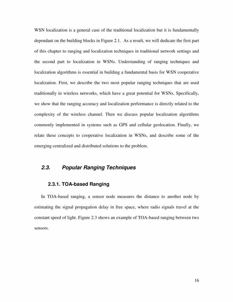
17
Figure 2.3: TOA ranging between sensors. The TOA can be measured by recording the time
it takes to transmit and receive a packet between two nodes. If however, the direct path
signal is block then the time delay or distance estimation is biased which can cause
significant errors in the localization process.
The performance of TOA-based ranging depends on the availability of the DP signal
[Pah98, Pah02]. In its presence, such as short distance LOS conditions, accurate estimates
are feasible (see Figure 2.4).
1τ
2τ
LOS
NLOS/UDP
18
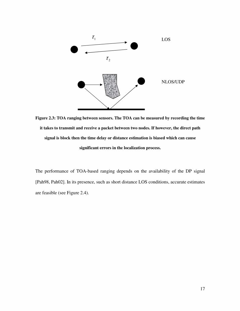
Figure 2.4: TOA estimation in the presence of DP. The accuracy of TOA estimation
depends on the availability of the DP signal. In this case, the DP signal power is well above
the detection threshold and thus can provide accurate distance estimation.
However, the challenge is ranging in NLOS conditions, which can be characterized as
site-specific and dense multipath environments [Pah98, Lee02]. These environments
introduce several challenges. The first, also present in LOS conditions, corrupts the TOA
estimates due to the multipath components (MPCs). MPCs are delayed and attenuated
replicas of the original signal, arriving and combining at the receiver thus shifting the
estimate. The second is the propagation delay caused by the signal traveling through
obstacles, which adds a positive bias to the TOA estimates. The third is the absence of the
DP due to blockage, also known as Undetected Direct Path (UDP) [Pah98]. The bias
imposed by this type of error is usually much larger than the first two and has a
significant probability of occurrence due to cabinets, elevator shafts, or doors that are
19
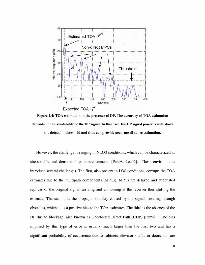
usually cluttering the indoor environment. A sample measurement profile of this
condition is illustrated in Figure 2.5 which illustrates TOA ranging in the absence of the
DP.
Figure 2.5: TOA estimation in the absence of the DP. In this condition, the DP signal power
is attenuated and cannot be detected. As a result the first arriving path is used for TOA
ranging instead causing significant estimation errors.
As a result for effective TOA-based ranging and localization it is important for a node
to be able to distinguish between these two cases. Although TOA-based systems are more
accurate compared to RSS or AOA systems, their implementation is usually more
complex and they suffer severely in impaired indoor environments.
20
2.3.2. RSS-based Ranging
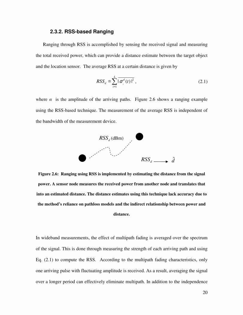
Ranging through RSS is accomplished by sensing the received signal and measuring
the total received power, which can provide a distance estimate between the target object
and the location sensor. The average RSS at a certain distance is given by
2
1
| ( ) |i
Ld
d
i
RSS tα=
=∑ , (2.1)
where α is the amplitude of the arriving paths. Figure 2.6 shows a ranging example
using the RSS-based technique. The measurement of the average RSS is independent of
the bandwidth of the measurement device.
Figure 2.6: Ranging using RSS is implemented by estimating the distance from the signal
power. A sensor node measures the received power from another node and translates that
into an estimated distance. The distance estimates using this technique lack accuracy due to
the method’s reliance on pathloss models and the indirect relationship between power and
distance.
In wideband measurements, the effect of multipath fading is averaged over the spectrum
of the signal. This is done through measuring the strength of each arriving path and using
Eq. (2.1) to compute the RSS. According to the multipath fading characteristics, only
one arriving pulse with fluctuating amplitude is received. As a result, averaging the signal
over a longer period can effectively eliminate multipath. In addition to the independence
dRSS (dBm)
d dRSS
21
of the ranging error in RSS to the system bandwidth, this technique is relatively simple
and reliable. Nonetheless, the relationship between the measured RSS and the distance is
complex and diversified. Therefore, the performance of these techniques depends on the
accuracy of the model used for estimation of the RSS.
A number of statistical models relating the behavior of the RSS to the distance
between a transmitter and a receiver in indoor areas have been developed for wireless
communications [Pah02]. These models can be used for estimating the ranging distance
between two nodes. The common principle behind all statistical models for calculation of
the RSS in a distance d is given by
10 10 1010log 10log 10 logd r t
RSS P P d Xγ= = − + , (2.2)
where Pt is the transmitted power, d is the distance between the transmitter and the
receiver, γ is the so-called distance-power gradient of the environment, and X is a
lognormal random variable representing the shadow fading component. Since the
location sensor using RSS does not know the exact value of γ and X, the distance
calculated from these models is not as reliable as its TOA counterpart.
2.4. Wireless Localization Algorithms
2.4.1. Background
Using range estimates from multiple anchors, it is possible to employ simple
geometrical triangulation techniques to estimate the location of a sensor. Due to
estimation errors in the acquired TOA ranges, for example, the geometrical triangulation
technique can only provide a region of uncertainty, instead of a single position fix for a
22
sensor node. To obtain an estimate of the location coordinates, a variety of direct and
iterative statistical positioning algorithms have been developed to solve the problem by
formulating it into a set of non-linear iterative equations. In some wireless geolocation
applications, the purpose of the positioning systems is to provide a visualization of the
possible mobile locations instead of an estimate of the location coordinates. In either
case, the position accuracy is not constant across the area of coverage and poor geometry
of relative position of the mobile terminal and RPs can lead to high geometric dilution of
precision (GDOP). Further, geometric and statistical triangulation algorithms are used
when both the region of uncertainty and the estimate of the location are required [Kap96].
Localization algorithms with well-defined properties, such as the least squares (LS)
algorithm and maximum-likelihood algorithm, are available for satellite-based GPS
systems. In addition, there are various types of sequential filters, including formulations,
which adaptively estimate some unknown parameters of the noise processes [Mis02,
Kap96]. In particular, GPS has focused a great deal of attention on positioning algorithms
based on TOA with considerable success. GPS can provide positioning accuracy ranging
from tens of meters to centimeters in real time depending upon a user’s resources
[Mis02]. In essence, these techniques are readily applicable to indoor location sensing
systems. However, indoor location sensing involves quasi-stationary applications and a
number of unreliable reference points for which the existing GPS algorithms, designed
for mobile systems with a few reliable reference points, do not provide the optimum
solution.
Geometrical techniques are based on iterative algorithms that estimate the node
position by formulating and solving a set of non-linear equations. When the statistics of
23
the ranging error, be it TOA or RSS, are not available a priori, the LS algorithms can
provide the best solution. However, if the statistics of the ranging error are available, a
WLS algorithm can be implemented, which weighs the range measurements with the
variance of the respective error distributions. Thus the availability of the range error
information can substantially improve the accuracy of the localization process. Again, it
is important to realize that the distribution of the ranging error is directly related to the
RF wireless propagation channel.
2.4.2. Least Squares (LS) Algorithm
Estimating a node’s position in 2(3) dimensions requires range information to at least
3(4) anchors/RPs. For the sake of simplicity, we will provide an analysis for 2-
dimensional localization and an extension to higher dimensions can be easily obtained.
Let [ ],x y=θ be the sensor node’s x- and y-coordinates and let ,a a
i i ix y = φ denote the
coordinates of the ith anchor, where 1, ,i M∈ … . The range estimate between the ith
anchor and the sensor node is then given by
( ) ( )2 2ˆ a a a
i i i i i i i id z x x y y zε ε= − + + = − + − + +θ φ ɶ ɶ , (2.3)
where i
ε is the ranging error and i
zɶ is additive measurement noise. Note that the
statistics of i
ε are not necessarily identically distributed. In indoor environments, the
ranging error will experience different means and variances depending on the distances
between the nodes and the blockage condition. Also for the sake of simplicity and noting
that the errors induced by the channel are substantially more significant than
synchronization errors, we assume that the nodes involved in localization are
synchronized. Given M noisy measurements to respective anchors, it is possible to obtain
24
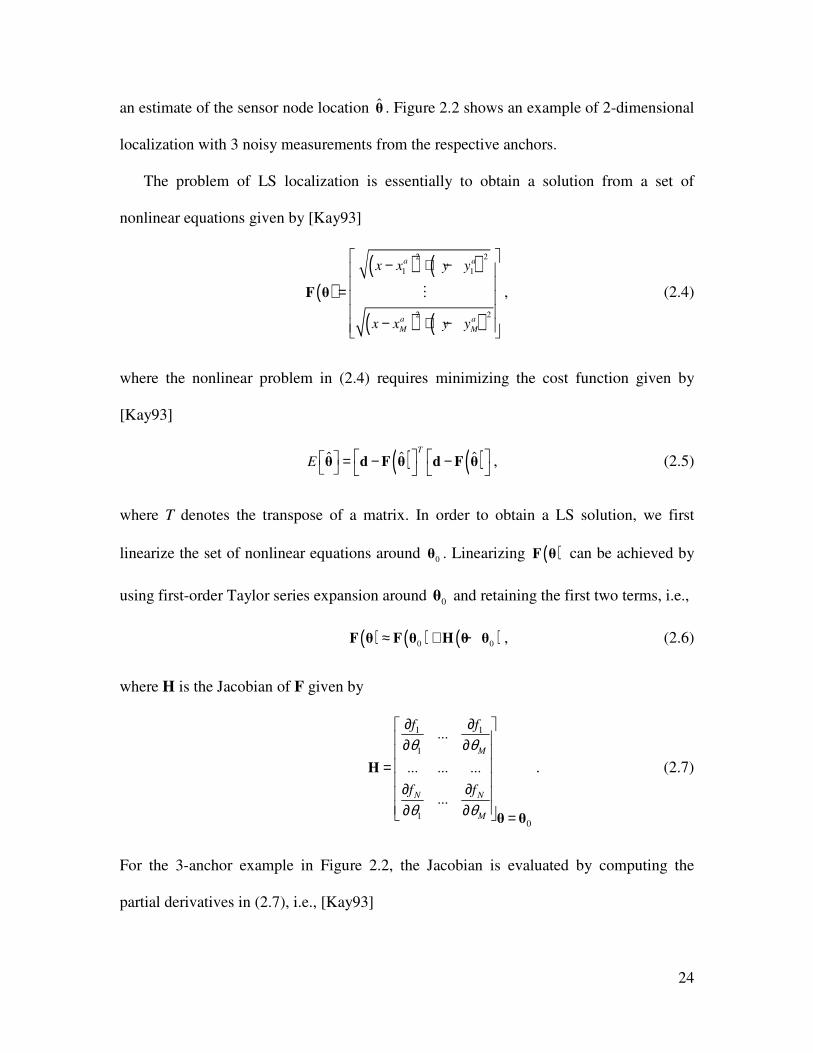
an estimate of the sensor node location θ . Figure 2.2 shows an example of 2-dimensional
localization with 3 noisy measurements from the respective anchors.
The problem of LS localization is essentially to obtain a solution from a set of
nonlinear equations given by [Kay93]
( )( ) ( )
( ) ( )
2 2
1 1
2 2
a a
a a
M M
x x y y
x x y y
− + − =
− + −
F θ ⋮ , (2.4)
where the nonlinear problem in (2.4) requires minimizing the cost function given by
[Kay93]
( ) ( )ˆ ˆ ˆT
E = − − θ d F θ d F θ , (2.5)
where T denotes the transpose of a matrix. In order to obtain a LS solution, we first
linearize the set of nonlinear equations around 0θ . Linearizing ( )F θ can be achieved by
using first-order Taylor series expansion around 0θ and retaining the first two terms, i.e.,
( ) ( ) ( )0 0≈ + −F θ F θ H θ θ , (2.6)
where H is the Jacobian of F given by
1 1
1
10
...
... ... ...
...
M
N N
M
f f
f f
θ θ
θ θ
∂ ∂ ∂ ∂ = ∂ ∂ ∂ ∂ =
H
θ θ
. (2.7)
For the 3-anchor example in Figure 2.2, the Jacobian is evaluated by computing the
partial derivatives in (2.7), i.e., [Kay93]
25
( ) ( ) ( ) ( )
( ) ( ) ( ) ( )
( ) ( ) ( ) ( )
1 1
2 2 2 21 1
1 1 1 1
2 2 2 2
2 2 2 2
2 2 2 2
3 3
3 3
2 2 2 2
3 3 3 3
a a
a a a a
a a
a a a a
a a
a a a a
x x y yf f
x x y y x x y yx y
f f x x y y
x yx x y y x x y y
f fx x y y
x y
x x y y x x y y
− −
∂ ∂ − + − − + − ∂ ∂ ∂ ∂ − −= = ∂ ∂ − + − − + − ∂ ∂ − −∂ ∂
− + − − + −
H . (2.8)
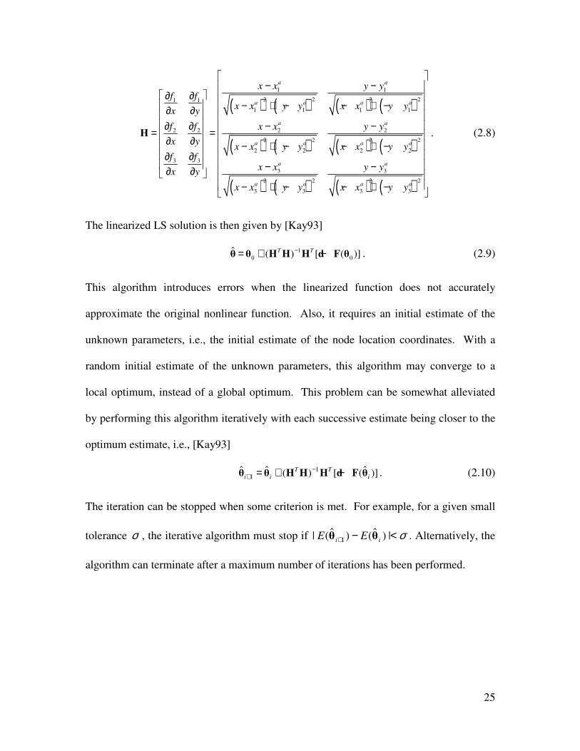
The linearized LS solution is then given by [Kay93]
1
0 0ˆ ( ) [ ( )]T T−= + −θ θ H H H d F θ . (2.9)
This algorithm introduces errors when the linearized function does not accurately
approximate the original nonlinear function. Also, it requires an initial estimate of the
unknown parameters, i.e., the initial estimate of the node location coordinates. With a
random initial estimate of the unknown parameters, this algorithm may converge to a
local optimum, instead of a global optimum. This problem can be somewhat alleviated
by performing this algorithm iteratively with each successive estimate being closer to the
optimum estimate, i.e., [Kay93]
11
ˆ ˆ ˆ( ) [ ( )]T Ti i i
−+ = + −θ θ H H H d F θ . (2.10)
The iteration can be stopped when some criterion is met. For example, for a given small
tolerance σ , the iterative algorithm must stop if σ<−+ |)ˆ()ˆ(| 1 ii EE θθ . Alternatively, the
algorithm can terminate after a maximum number of iterations has been performed.
26
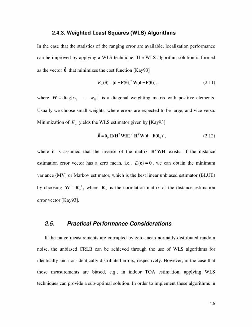
2.4.3. Weighted Least Squares (WLS) Algorithms
In the case that the statistics of the ranging error are available, localization performance
can be improved by applying a WLS technique. The WLS algorithm solution is formed
as the vector θ that minimizes the cost function [Kay93]
ˆ ˆ ˆ( ) [ ( )] [ ( )]TwE = − −θ d F θ W d F θ , (2.11)
where ...diag 1 Nww=W is a diagonal weighting matrix with positive elements.
Usually we choose small weights, where errors are expected to be large, and vice versa.
Minimization of wE yields the WLS estimator given by [Kay93]
10 0
ˆ ( ) [ ( )]T T−= + −θ θ H WH H W d F θ , (2.12)
where it is assumed that the inverse of the matrix TH WH exists. If the distance
estimation error vector has a zero mean, i.e., 0e =E , we can obtain the minimum
variance (MV) or Markov estimator, which is the best linear unbiased estimator (BLUE)
by choosing 1−= eRW , where eR is the correlation matrix of the distance estimation
error vector [Kay93].
2.5. Practical Performance Considerations
If the range measurements are corrupted by zero-mean normally-distributed random
noise, the unbiased CRLB can be achieved through the use of WLS algorithms for
identically and non-identically distributed errors, respectively. However, in the case that
those measurements are biased, e.g., in indoor TOA estimation, applying WLS
techniques can provide a sub-optimal solution. In order to implement these algorithms in
27
the indoor environments, the statistics of the bias must be incorporated. Obtaining the
statistics of the bias in indoor environments requires extensive TOA-based ranging
measurements and modeling campaigns [Als07b]. In addition, identification of NLOS on
specific range measurements must be integrated with mitigation techniques that adjust the
weights in WLS to improve the localization accuracy [Che99].
Another factor affecting the quality of location estimation is the geometry of the
anchors relative to the sensor node. GDOP is commonly used in localization applications
to quantify the geometrical impact on precision. The GDOP expression has many
different forms [Kap96], but a simple expression in terms of the angles between the
anchors and the sensor node is given by [Spi01]
( )( ) 2
,
sin iji jj i
MGDOP M φ
φ>
=∑ ∑
, (2.11)
where M is the number of anchors involved in the localization process and φ is the angle
between each pair of anchors. An example illustrating the impact of geometry on the
precision of localization is given in Figure 2.7. In this simulation example, the statistics
of the ranging error between the node and the anchors are identical.
28
Figure 2.7: Effect of geometry on sensor node position estimation: (a) Good geometry – the
anchors evenly surround the sensor node. As a result, the location accuracy is high since the
GDOP is minimized according to eq (2.11) (b) Bad geometry – when the anchors are very
close to each other GDOP is high and that results in lower location accuracy characterized
by the “smearing” of the location estimates.
In Figure 2.7 (a), the anchors are at 120o relative to each other. While in Figure 2.7 (b),
they are 20o apart. The figure highlights the impact of geometry on the precision, where
the effect of sensor node and anchor geometry can be clearly seen. The spreading of the
ranging error in the 20o case results in higher uncertainty.
2.6. Cooperative Localization in WSNs
2.6.1. Background
The previous sections provided an understanding of the different traditional
approaches to the localization problem. It is evident that the localization accuracy
(a) (b)
29
depends on the ranging technique employed, deployment environment (which affects the
ranging error statistics), and the relative geometry of the sensor node to the anchors. The
major difference between traditional localization and WSN localization is cooperative
localization. Cooperative localization refers to the collaboration between sensor nodes to
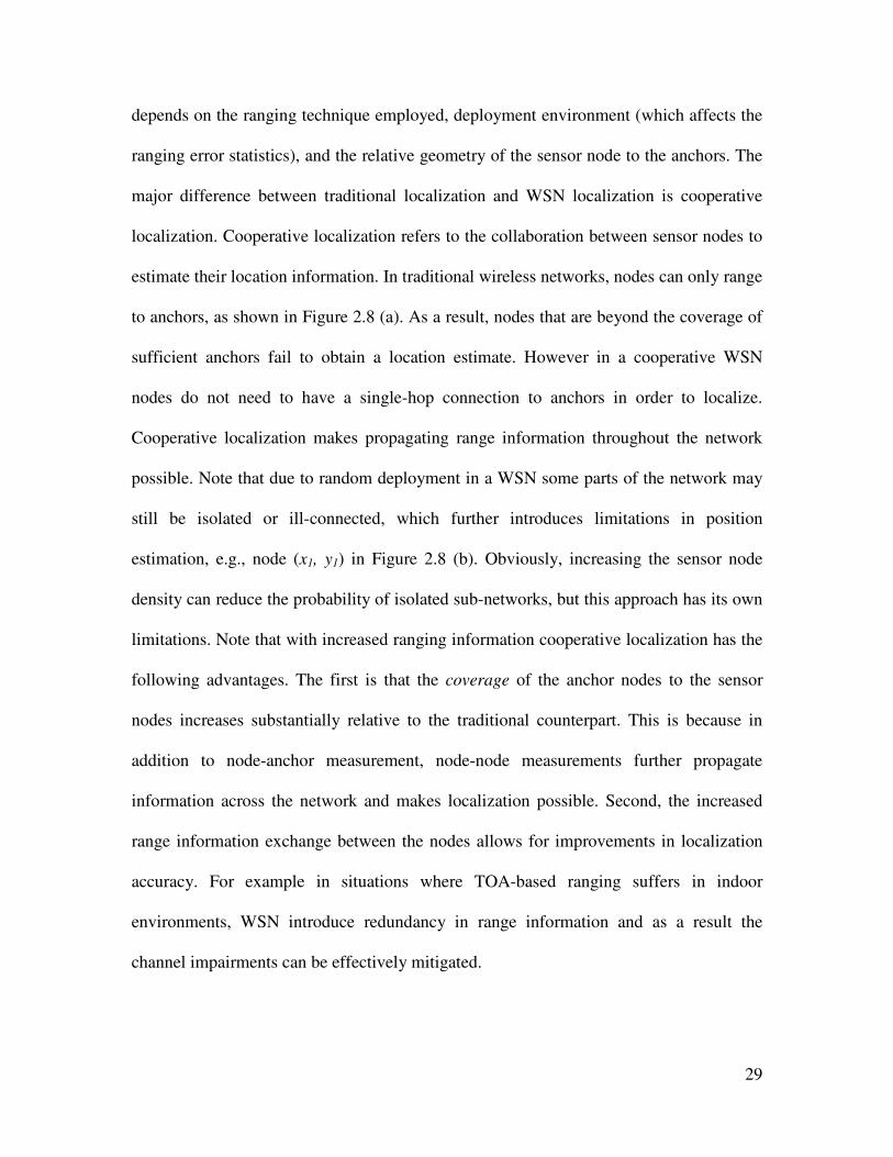
estimate their location information. In traditional wireless networks, nodes can only range
to anchors, as shown in Figure 2.8 (a). As a result, nodes that are beyond the coverage of
sufficient anchors fail to obtain a location estimate. However in a cooperative WSN
nodes do not need to have a single-hop connection to anchors in order to localize.
Cooperative localization makes propagating range information throughout the network
possible. Note that due to random deployment in a WSN some parts of the network may
still be isolated or ill-connected, which further introduces limitations in position
estimation, e.g., node (x1, y1) in Figure 2.8 (b). Obviously, increasing the sensor node
density can reduce the probability of isolated sub-networks, but this approach has its own
limitations. Note that with increased ranging information cooperative localization has the
following advantages. The first is that the coverage of the anchor nodes to the sensor
nodes increases substantially relative to the traditional counterpart. This is because in
addition to node-anchor measurement, node-node measurements further propagate
information across the network and makes localization possible. Second, the increased
range information exchange between the nodes allows for improvements in localization
accuracy. For example in situations where TOA-based ranging suffers in indoor
environments, WSN introduce redundancy in range information and as a result the
channel impairments can be effectively mitigated.
30
Figure 2.8: Cooperative localization concept in WSN. (a) Traditional wireless networks. (b)
WSNs. Black circles are anchor nodes and white circles are “blind” sensor nodes. In WSNs
the cooperation between the sensor nodes allows for increased information sharing. This
specifically provides enhanced coverage and improvement in localization accuracy.
(x1,y1)
(x2,y2) (x3,y3)
(x9,y9)
(x4,y4)
(x5,y5) (x6,y6)
(x7,y7)
(x8,y8)
(x10,y10)
(x11,y11)
(x1,y1)
(x2,y2) (x3,y3)
(x9,y9)
(x4,y4)
(x5,y5) (x6,y6)
(x7,y7)
(x8,y8)
(x10,y10)
(x11,y11)
(a)
(b)
31
2.6.2. Cooperative Localization Techniques
In general, there are two main approaches to node localization in WSNs. The first is
centralized and the second is distributed. In both approaches absolute and relative
localization is possible. Unlike relative localization, in absolute localization anchor nodes
are needed in order to provide a global frame of reference. Anchors or beacons are sensor
nodes that are aware of their locations (usually through GPS or pre-programmed during
setup) and they are necessary for WSN applications that require localization with respect
to an absolute global frame of reference, e.g., GPS. Depending on the desired application,
either relative or absolute cooperative localization is possible. In this section we briefly
provide an overview and highlight the differences between centralized and cooperative
localization techniques.
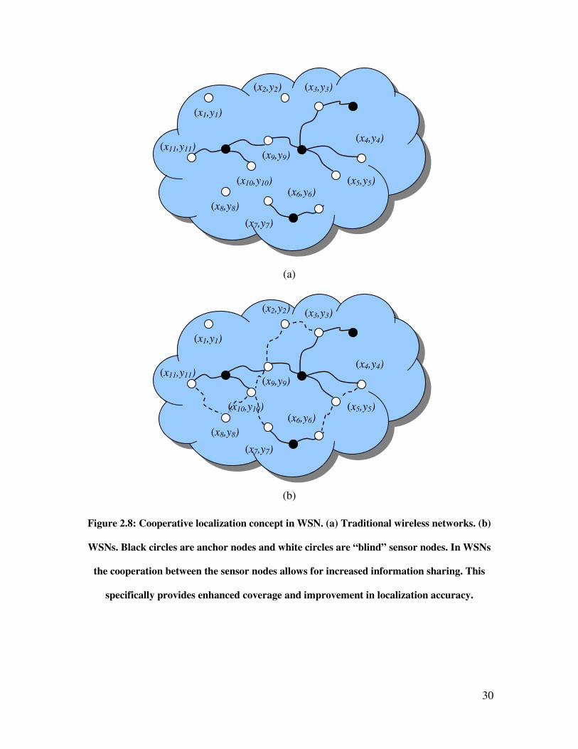
In centralized localization, information of each node in the network is determined
centrally through a computer usually at one edge of the network. The range estimates
between all node pairs in the network are forwarded to the processing unit, where a
complex centralized algorithm estimates the location of each node in the network. Figure
2.9 (a) illustrates the centralized approach. The advantage of this technique is that all
ranging information between node pairs is available to the central processor. As a result,
the processor has a top-level view of the connectivity of the network. The amount of
information allows the centralized algorithm to generate more accurate localization
results. The drawbacks, on the other hand, include traffic congestion and computational
complexities, especially for larger sensor networks. In the former, the possibility of
congestion that occurs close to the central processing unit due to information going back
and forth can reduce the effectiveness of this approach. Similarly, the latter drawback
32
imposes constraints on the computation time needed to handle estimating the node
positions in a large WSN.
Figure 2.9: WSN localization: (a) centralized, (b) distributed.
The second approach used in WSN localization is distributed in nature (see Figure 2.9
(b)). The process is usually iterative, where sensor nodes attempt to localize themselves
first and then aid the reminder of the nodes in the localization process. Distributed
positioning algorithms provide the best alternatives so far in their approach. The
algorithms are self-organizing and energy efficient.
2.6.3. Challenges Facing Distributed Localization Algorithms
In this dissertation, we will focus on distributed localization algorithms, mainly due to
their simplicity in implementation and to their robustness to TOA-based ranging errors.
In this subsection we briefly overview the major challenges facing WSN localization.
These challenges can be categorized into network and channel parameters.
(a)
Ranging
information Sensor node location
estimates
(b)
Localization achieved
within the WSN
33
When considering network parameters, localization is mainly constrained by the size
(i.e., the number of nodes and anchors), the topology, and the connectivity of the
network. Network connectivity is determined by node density, which is usually defined
as the number of nodes per square meter (nodes/m2). A network with a high node density
exhibits improved localization performance compared to a sparse networks. Further, in
sparse WSNs there is a high probability of ill-connected or isolated nodes and in such
cases localization accuracy can be degraded substantially. Therefore, it is always
desirable to increase the node density (higher connectivity information means a lower
probability of ill-connected networks) to improve the accuracy of localization. However,
with increased sensor nodes, the error can substantially propagate from one hop to the
next, which can be a serious problem in WSN distributed localization algorithms. This
phenomenon is known as error propagation and it is caused by the iterative nature of
these distributed algorithms. When a node transforms into an anchor, the error in the
range estimates used in the localization process impacts its position estimate. When other
nodes in the network use this newly transformed anchor, the position error will propagate
to the new node’s position estimate. Therefore, in several iterative steps, error
propagation can substantially degrade the localization performance.
The second and most limiting factor affecting WSN localization is the wireless RF
channel. Effective cooperative localization hinges on the RF ranging technology and its
behavior in the deployed environment. The TOA techniques have been widely accepted
as the most accurate but their behavior varies significantly in different deployment
environments. For example, deploying hundreds of nodes in outdoor environments
presents different challenges relative to trying to locate sensors inside a building. In
34
particular, WSNs in indoor areas face severe multipath fading and harsh radio
propagation, causing large ranging estimation errors that impact localization performance
directly. To develop practical and accurate cooperative localization algorithms, the
behavior of the wireless channel must be first investigated and then integrated into the
algorithm. Specifically, the localization algorithms must assess the quality of the ranging
estimates and integrate that information into the localization process to further provide
robust iterative performance.
35
Chapter 3 UWB TOA-based Ranging:
Concepts, Measurements & Modeling
3.1. Background
Recently, UWB technology has been one of the major developments in the wireless
industry with potential for high data-rate communication and precise TOA based ranging
[Por03, Ghav04, Opp04]. Large bandwidth offers high resolution and signaling which
allows for centimeter accuracies, low-power and low-cost implementation [Gez05].
Numerous potential applications have been identified for indoor localization in general
and for UWB localization in particular [Gez05, Pah02, Fon02]. Depending on the nature
of the application different ranging scenarios will be necessary for both traditional and
WSNs. This means that scenarios will not be limited to indoor-to-indoor (ITI) ranging.
Indeed for a variety of applications (e.g. firefighters, soldiers in hostile buildings) rapid
deployment of beacon infrastructure surrounding and on top of buildings will be
necessary. In these situations outdoor-to-indoor (OTI) and roof-to-indoor (RTI) will
impose different challenges to UWB ranging (see Figure 3.1).
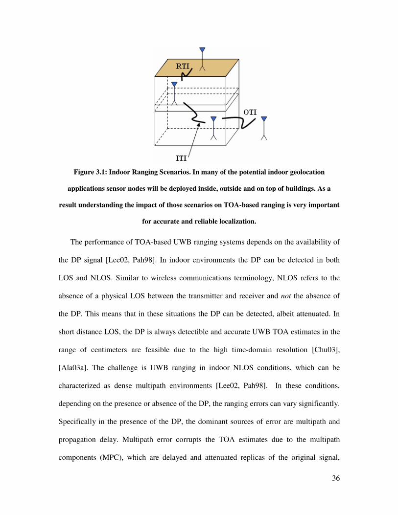
36
Figure 3.1: Indoor Ranging Scenarios. In many of the potential indoor geolocation
applications sensor nodes will be deployed inside, outside and on top of buildings. As a
result understanding the impact of those scenarios on TOA-based ranging is very important
for accurate and reliable localization.
The performance of TOA-based UWB ranging systems depends on the availability of
the DP signal [Lee02, Pah98]. In indoor environments the DP can be detected in both
LOS and NLOS. Similar to wireless communications terminology, NLOS refers to the
absence of a physical LOS between the transmitter and receiver and not the absence of
the DP. This means that in these situations the DP can be detected, albeit attenuated. In
short distance LOS, the DP is always detectible and accurate UWB TOA estimates in the
range of centimeters are feasible due to the high time-domain resolution [Chu03],
[Ala03a]. The challenge is UWB ranging in indoor NLOS conditions, which can be
characterized as dense multipath environments [Lee02, Pah98]. In these conditions,
depending on the presence or absence of the DP, the ranging errors can vary significantly.
Specifically in the presence of the DP, the dominant sources of error are multipath and
propagation delay. Multipath error corrupts the TOA estimates due to the multipath
components (MPC), which are delayed and attenuated replicas of the original signal,
37
arriving and combining at the receiver shifting the estimate. Propagation delay, caused by
the signal traveling through obstacles, can further add a positive bias to the TOA
estimates. Although UWB can mitigate multipath with the availability of excess
bandwidth [Ala03a, Tar06] its ability to perform in the absence of the DP needs to be
further investigated. In the absence of the DP, also referred to as Undetected Direct Path
(UDP) in [Pah98, Pah06], Type 1 and Type 2 NLOS in [Den04] and late errors in
[Lee06], range estimates are corrupted by larger positive biases which have a significant
probability of occurrence due to cabinets, elevator shafts, or doors that are usually
cluttering the indoor environment. Furthermore, mitigation of this problem through
increasing the system bandwidth alone has its limitation [Pah06].
Characterization of the UWB channels for ranging applications is different from
communications [Pah02]. For the latter, the focus is on data rate and communication
coverage through characterization of the delay spread and the pathloss of the total signal
energy. However, the former requires special attention on the ranging accuracy, i.e.
statistics of the ranging error, and ranging coverage. Characterizing the probability of DP
blockage and the statistics of the error in the presence and absence of the DP provides an
understanding of the challenges and limitations imposed by the multipath environment.
For the ranging coverage, characterizing the pathloss-distance dependence of the DP in a
given scenario and environment can provide practical indications of the maximum
possible ranging distance [Als07a].
UWB indoor propagation experiments have been carried out extensively [Mol05,
Gha04, Muq06, Cho05], but these efforts focus mainly on the communication aspects of
UWB. Several indoor propagation experiments with a focus on indoor ranging, be it
38
UWB or otherwise, have been reported in [Fon02, Lee02, Pah98, Ala03a, Tar06, Den04,
Fal06, Ala06, Pat03, Hat06, Ala05, Low05], where experiments are usually limited to a
floor or several rooms but do not address modeling the spatial statistics of NLOS ranging
or ranging coverage. The only available ranging error models were provided in [Den04,
Ala06] but are based on limited measurement data sets, and only the latter focuses on
characterization of errors according to the availability of the DP. As a result a
comprehensive measurement and modeling of the UWB TOA-based ranging in different
indoor environments and scenarios is not available in the literature. These models are
needed to provide a realistic platform for algorithm performance analysis. More
importantly, they are necessary for determining localization performance bounds in
NLOS cluttered environments [Qi06], [Jou06a] which can provide insight into the
fundamental limitations facing indoor UWB localization in both traditional wireless
networks and sensor networks.
3.2. UWB TOA-based Ranging Concepts
UWB TOA-based ranging can be achieved through different technologies. There are,
however, two promising solutions, namely, Multi-band Orthogonal Division
Multiplexing (MBOFDM) and single pulse transmission. In the former, the OFDM
modulated signal contains parallel transmissions of signals that are modulated at
orthogonally spaced frequency carriers. Specifically in the 802.15.3a MB-OFDM
standard, the UWB band is divided into 14-sub-bands. Each sub-band provides ranging
with 528 MHz bandwidth capability [Bet04]. In the latter technique very narrow time-
domain pulses have bandwidths in excess of 1 GHz provide even better time-domain

39
resolution [Lee02]. In this dissertation we will focus on the TOA-based ranging
capabilities of these two promising systems. Specifically our results and analysis will be
focused on two different system bandwidths 500MHz and 3 GHz resembling the MB-
OFDM and pulse-based respectively.
One of the major factors determining the quality of TOA-based ranging in indoor
geolocation is the ability to detect the DP between a RP and a MT in the presence of
dense multipath. For the indoor multipath channel, the impulse response is usually
modeled as,
∑=
−=p
k
L
k
k
j
k eh1
)()( ττδατ φ (3.1)
where pL is the number of MPCs, and kα , kφ and kτ are amplitude, phase and
propagation delay of the kth
path, respectively [Pah05]. When the DP is detected
1 DPα α= and 1 DP
τ τ= where DP
α and DP
τ denote the DP amplitude and propagation
delay, respectively. Figures 2.4 and 2.5 provide sample measured channel profile and the
relative amplitude and delay of the MPCs. The distance between the MT and the RP is
DP DPd v τ= × , where v is the speed of signal propagation. In the absence of the DP,
ranging can be achieved using the amplitude and propagation delay of the first Non-
Direct Path (NDP) component given by NDP
α and NDP
τ respectively; resulting in a longer
distance given by NDP NDP
d v τ= × where NDP DP
d d> . For the receiver to identify the DP,
the ratio of the strongest MPC to the DP given by
( )1
1
maxpL
i i
DP
αρ
α=
=
(3.2)
40
must be less than the receiver dynamic range ρ and the power of the DP must be greater
than the receiver sensitivity ϕ [Kri99]. These constraints are given by,
1ρ ρ≤ (3.3a)
ϕ>DPP (3.3b)
where ( )1020logDP DP
P α= .
3.2.1. Ranging Coverage
The performance of UWB TOA-based ranging is then constrained by the maximum
feasible distance where DP
P can satisfy (3.3a) and (3.3b). This is analogous to the
dependence of a communication system’s performance on the distance relationship of the
total signal energy of all the detectable MPCs, or ( )10 120log
pL
T kkP α
== ∑ . In indoor
environments, the distance-dependence of T
P , which determines the limitations of
communication coverage, is usually predicted from experimental pathloss models of the
total signal energy in different environments and scenarios [Dur98, Mol05, Gha04].
Similarly, the distance-dependence behavior of DP
P is important in analyzing the physical
limitations facing UWB TOA-based ranging. These indoor radio wave propagation
measurements have focused mainly on determining the radio coverage in different
environments. However, the reported results and models are not adequate for predicting
the coverage of TOA-based UWB indoor geolocation systems because the performance
in multipath rich indoor environments depends on the signal-to-noise (SNR) of the DP
between the transmitter and the receiver. Unlike communication coverage which is
related to the received power of all the MPCs in a given distance, ranging coverage is
41
related to the received power of the DP component. For a given system dynamic range,
ρ , we define ranging coverage, cR , as the distance in which the maximum tolerable
average pathloss of the DP is within ρ [Als07a]. This is represented by
10max 10 log ( )DP c
PL Rγ ρ= ≤ (3.4)
where DPPL is the average pathloss of the DP and γ is the pathloss exponent. The
pathloss behavior of the DP is distance-dependant but because of attenuation and energy
removed by scattering its intensity decreases more rapidly with distance compared with
the total signal energy [Siw03]. This means that for typical indoor multipath scattering
environment communication coverage is greater than ranging coverage, c c
C R> .
Operating out of ranging coverage causes large TOA estimation errors and performance
degradation.
In general, ranging coverage in indoor multipath environments depends on the
channel condition between a pair of nodes. The channel condition is physically
constrained by the environment and the scenario. The environment refers to the type of
building such as residential, manufacturing or office. The scenario refers to the relative
location of the node-node or anchor-node pair which can be grouped into the following:
ITI, OTI, and RTI. In ITI ranging the pathloss behavior varies significantly between LOS
and NLOS channel conditions. In the latter, ranging coverage is reduced due to
penetration loss caused by the interior wall structures, which results in a higher DP
pathloss exponent. Similarly OTI and RTI ranging imposes harsher constraints on the
pathloss, due to the DP having to penetrate the outside walls and roof respectively, which
42
means that ITI OTI RTI
c c cR R R> > [Als07a]. This poses a challenge specifically for indoor
localization in ad-hoc and WSN applications.
3.2.2. Ranging Error
Ranging and localization are further constrained by the statistics of the ranging error.
Ranging error is defined as the difference between the estimated and the actual distance
or
ˆDP
d dε = − . (3.5)
where d is the estimated distance and DP
d is the actual distance. In an indoor
environment the MT experiences varying ranging error behavior depending on the
relative location of the MT to that of the RP. More specifically it depends on the
availability of the DP and in the case of its absence on the characteristics of the blockage.
In this dissertation we categorize the error based on the following ranging states. In the
presence of the DP, both (3.3a) and (3.3b) are met and the distance estimate is very
accurate yielding
ˆDP DP DP
d d nε= + + (3.6a)
( )( )
m
DP
m pd
b LOS
b b NLOS
ωε
ω= +
(3.6b)
where ( )mb ω is the bias induced by the multipath that dominates when the DP is present
and it is a function of the system’s bandwidth, ω [Ala03a, Tar06]. pd
b is the propagation
delay imposed by the NLOS condition. n is zero mean Gaussian measurement noise.
Similar to wireless communications terminology, we will use the NLOS term to denote
43
the absence of a physical LOS between the transmitter and receiver and not the absence
of the DP. This means that in these situations the DP can be detected, albeit attenuated.
When the MT is within ranging coverage but experiences sudden blockage of the DP,
also known as UDP [Pah98], (3.3a) is not met and the DP is shadowed by some obstacle
burying its power under the dynamic range of the receiver. In this situation, the ranging
estimate experiences a larger bias error compared to (3.6). Emphasizing that ranging is
achieved through NDP component, the estimate is then given by
ˆNDP DP NDP
d d nε= + + (3.7a)
( ) ( )NDP m pd Bb b bε ω ω= + + (3.7b)
where ( )Bb ω is positive, additive bias representing the nature of the blockage, and it
dominates the error compared to measurement noise. Its dependence on bandwidth is
through its impact on the energy per MPC. Higher bandwidth results in lower energy per
MPC which increases the probability of DP blockage. Finally, when the user operates
outside of the ranging coverage neither (3.3a) nor (3.3b) is met and large errors occur
with high probability.
Formally, these ranging states can be defined as follows,
cDP Rddd ≤== |ˆˆ1ζ (3.8a)
cNDP Rddd ≤== |ˆˆ2ζ (3.8b)
cNDP Rddd >== |ˆˆ3ζ (3.8c)
cDP Rddd >== |ˆˆ4ζ (3.8d)
44
In this dissertation we will focus on modeling the error statistics within the ranging
coverage. The performance in 3ζ is dominated by large measurement noise variations
which means the significance of (3.6b) and (3.7b) diminishes [Jou06a]. We further
assume that 0)( 4 ≈ζp since from our definition in (3.4) the DP cannot be detected after
the ranging coverage.
3.2.3. Factors Affecting Ranging Coverage and Accuracy
Both ranging coverage and accuracy are functions of system dynamic range,
bandwidth, physical building environment and ranging scenario. Physical environment
refers to the type of the building: residential, office or manufacturing floor. Ranging
scenario refers to the location of the transmitter with respect to the receiver. Several
scenarios are common in potential indoor geolocation applications. Figure 3.1 shows a
typical multi-story building with three main ranging scenarios: ITI, OTI and RTI where
the last two can be primarily used in firefighter or military applications where ad-hoc
deployments are more practical. Ranging coverage is affected directly through the
attenuation induced on the DP which is dependent on the environment and scenario. For
example, residential environments, primarily composed of wooden structures, pose
different attenuation characteristics compared to office buildings which are composed of
concrete and metallic beam structures. In addition penetration loss due to exterior walls is
higher than interior walls which mean that ITI, OTI and RTI must impose different
physical constraints on the ranging performance. The impact of ranging environment and
scenarios on the accuracy, however, can be attributed to multipath and probability of DP
blockage. The harsher the indoor environment the higher the multipath error and the more
likely the DP would be shadowed by obstacles. Changes in system bandwidth affect
45
multipath and probability of DP blockage but increasing the system bandwidth arbitrarily
might reduce the former but emphasize the impact of the latter. Finally the impact of
SNR or dynamic range is rather intuitive but in reality UWB systems, due to FCC
regulations, face power constraints which make ranging under these conditions
challenging.
3.3. UWB Measurement Campaign
3.3.1. Background
Frequency domain measurement techniques have been previously employed to
characterize the channel impulse response [Gha04, Cho05, Pah05, How90]. The
measurements provided characterization of communication parameters such as the RMS
delay spread and power-distance relationship. In this dissertation we follow the same
techniques but measure the large-scale, spatial characteristics of the DP, mainly ˆDP
α and
ˆDP
τ which can be used to examine the ranging coverage (pathloss characterization) and
accuracy, respectively. In the absence of the DP we measure the first detected path, ˆNDP
τ
and analyze the probability of blockage and the error statistics in this condition.
3.3.2. Measurement System
The measurement system, similar to [Gha04, Cho05, How90], employs a 40GHz
Agilent E8363B vector network analyzer (VNA) that is used to sweep the frequency
spectrum of 3-8 GHz with 312.5 KHz sampling interval (16001 sampling points). The
VNA measures the S21 S-parameter which is the transfer function of the channel. The
transmitter and the receiver are a pair of disc-cone UWB antennas which are connected to
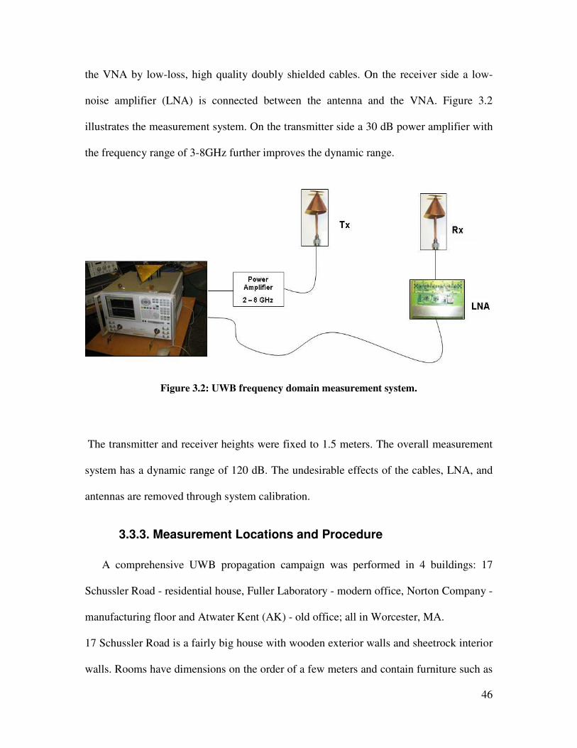
46
the VNA by low-loss, high quality doubly shielded cables. On the receiver side a low-
noise amplifier (LNA) is connected between the antenna and the VNA. Figure 3.2
illustrates the measurement system. On the transmitter side a 30 dB power amplifier with
the frequency range of 3-8GHz further improves the dynamic range.
Figure 3.2: UWB frequency domain measurement system.
The transmitter and receiver heights were fixed to 1.5 meters. The overall measurement
system has a dynamic range of 120 dB. The undesirable effects of the cables, LNA, and
antennas are removed through system calibration.
3.3.3. Measurement Locations and Procedure
A comprehensive UWB propagation campaign was performed in 4 buildings: 17
Schussler Road - residential house, Fuller Laboratory - modern office, Norton Company -
manufacturing floor and Atwater Kent (AK) - old office; all in Worcester, MA.
17 Schussler Road is a fairly big house with wooden exterior walls and sheetrock interior
walls. Rooms have dimensions on the order of a few meters and contain furniture such as

47
couches, tables, chairs, etc. Fuller Laboratories is a modern building characterized by
brick external walls with some aluminum siding on two sides, metallic window frames
and doors.
Table 3.1: Summary of the measurement database
Environment Scenario TX or RX
Location Description of the scenarios
Max.
meas.
range
(m)
Number of
Meas.
Entrance I/II Multi-floor – close to the door 336 OTI
Arbitrary Multi-floor – away from door 45
150
LOS Open area around entrance 24 120
Inter-floor – open area 72
Office (Fuller
Laboratories) ITI
NLOS Inter-floor – close area
23 54
Entrance I Multi-floor – front 186 OTI
Entrance II Multi-floor – side 15
186
Same-floor 108
Residential
(17 Schussler
Rd.) ITI NLOS Inter-floor
10 66
Entrance I Same-floor – close to the door 120 OTI
Entrance II Same-floor – away from door 38
126
LOS I Open area with machinery 120
Factory
(Norton
Company) ITI LOS II Straight walkway
40 126
OTI Entrance I /II Same-floor – main& side 27 132
ITI NLOS Rooms/corridors of 3rd
floor 26 90
AK3C Corridors of 3rd
floor 306
offices Small rooms 204
Office
(Atwater Kent
Laboratories) RTI
labs Large room
17
528
Total number of Measurements 3030
The dimension of the building is on the order of a few tens of meters and contains
several computer labs, department offices and lecture halls. Norton Company is a
manufacturer of welding equipment and abrasives for grinding machines with building
dimensions on the order of a few hundred meters and the floor is cluttered with machines,
equipment and metallic beams. The AK laboratory is a three floor building which has a
traditional office structure consisting of rooms that have dimensions in the order of few
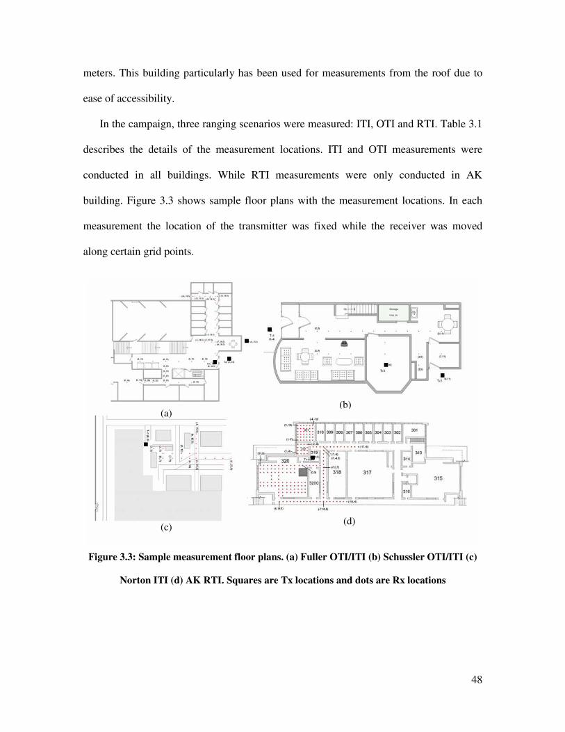
48
meters. This building particularly has been used for measurements from the roof due to
ease of accessibility.
In the campaign, three ranging scenarios were measured: ITI, OTI and RTI. Table 3.1
describes the details of the measurement locations. ITI and OTI measurements were
conducted in all buildings. While RTI measurements were only conducted in AK
building. Figure 3.3 shows sample floor plans with the measurement locations. In each
measurement the location of the transmitter was fixed while the receiver was moved
along certain grid points.
Figure 3.3: Sample measurement floor plans. (a) Fuller OTI/ITI (b) Schussler OTI/ITI (c)
Norton ITI (d) AK RTI. Squares are Tx locations and dots are Rx locations
(b) (a)
(c) (d)
49
Care was taken to conduct the measurements in a variety of indoor NLOS conditions
ranging from harsh obstacles such as elevator shafts, metallic doors and concrete walls to
other lighter wall structures as this would provide a wide variety of performance
conditions.
Measuring the behavior of the DP requires accurate a priori knowledge of the
transmitter-receiver distances. In the variety of locations we measured, this proved to be a
challenging task since there was no direct LOS. In order to cope with this problem we
devised a practical method to grid the building floor with transmitter and receiver
locations. We created a 3 dimensional Cartesian coordinate system with 1 meter as its
unit. Then we placed grid points on the floor in the positions that we were interested to
measure, and assigned x-, y-, and z-coordinates to each point. An extensive amount of
time and effort was placed in planning and carrying out this procedure in order to
minimize the error incurred from physically measuring the distance. For example, if the
coordinates of the transmitter and the receiver are given by ),,( AAA zyx and ),,( BBB zyx ,
respectively then the distance can be easily found using the Euclidian relation
222 )()()( BABABAAB zzyyxxd −+−+−= . (3.9)
3.3.4. Post-Processing
In the post-processing of channel measurement data, the time-domain channel
impulse response is obtained by first passing the frequency domain measurements
through a Hanning window in order to reduce the noise side lobes. Even though some
other window functions such as the Kaiser window provides higher dynamic range, the
Hanning window is selected for its much faster decaying side-lobes which significantly
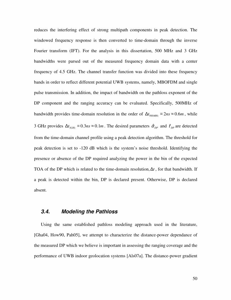
50
reduces the interfering effect of strong multipath components in peak detection. The
windowed frequency response is then converted to time-domain through the inverse
Fourier transform (IFT). For the analysis in this dissertation, 500 MHz and 3 GHz
bandwidths were parsed out of the measured frequency domain data with a center
frequency of 4.5 GHz. The channel transfer function was divided into these frequency
bands in order to reflect different potential UWB systems, namely, MBOFDM and single
pulse transmission. In addition, the impact of bandwidth on the pathloss exponent of the
DP component and the ranging accuracy can be evaluated. Specifically, 500MHz of
bandwidth provides time-domain resolution in the order of 500 2 0.6MHz
t ns m∆ = ≈ , while
3 GHz provides 3 0.3 0.1GHz
t ns m∆ = ≈ . The desired parameters ˆDP
α and ˆDP
τ are detected
from the time-domain channel profile using a peak detection algorithm. The threshold for
peak detection is set to -120 dB which is the system’s noise threshold. Identifying the
presence or absence of the DP required analyzing the power in the bin of the expected
TOA of the DP which is related to the time-domain resolution, t∆ , for that bandwidth. If
a peak is detected within the bin, DP is declared present. Otherwise, DP is declared
absent.
3.4. Modeling the Pathloss
Using the same established pathloss modeling approach used in the literature,
[Gha04, How90, Pah05], we attempt to characterize the distance-power dependance of
the measured DP which we believe is important in assessing the ranging coverage and the
performance of UWB indoor geolocation systems [Als07a]. The distance-power gradient
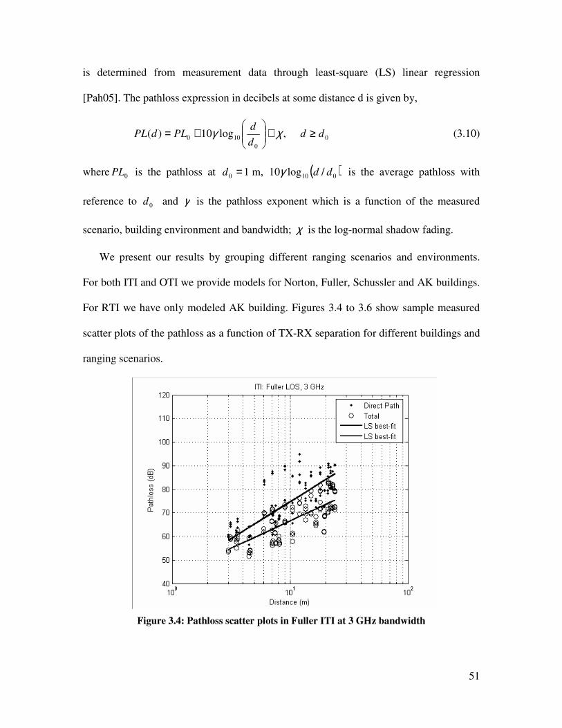
51
is determined from measurement data through least-square (LS) linear regression
[Pah05]. The pathloss expression in decibels at some distance d is given by,
0
0
100 ,log10)( ddd
dPLdPL ≥+
+= χγ (3.10)
where 0PL is the pathloss at 10 =d m, ( )010 /log10 ddγ is the average pathloss with
reference to 0d and γ is the pathloss exponent which is a function of the measured
scenario, building environment and bandwidth; χ is the log-normal shadow fading.
We present our results by grouping different ranging scenarios and environments.
For both ITI and OTI we provide models for Norton, Fuller, Schussler and AK buildings.
For RTI we have only modeled AK building. Figures 3.4 to 3.6 show sample measured
scatter plots of the pathloss as a function of TX-RX separation for different buildings and
ranging scenarios.
Figure 3.4: Pathloss scatter plots in Fuller ITI at 3 GHz bandwidth
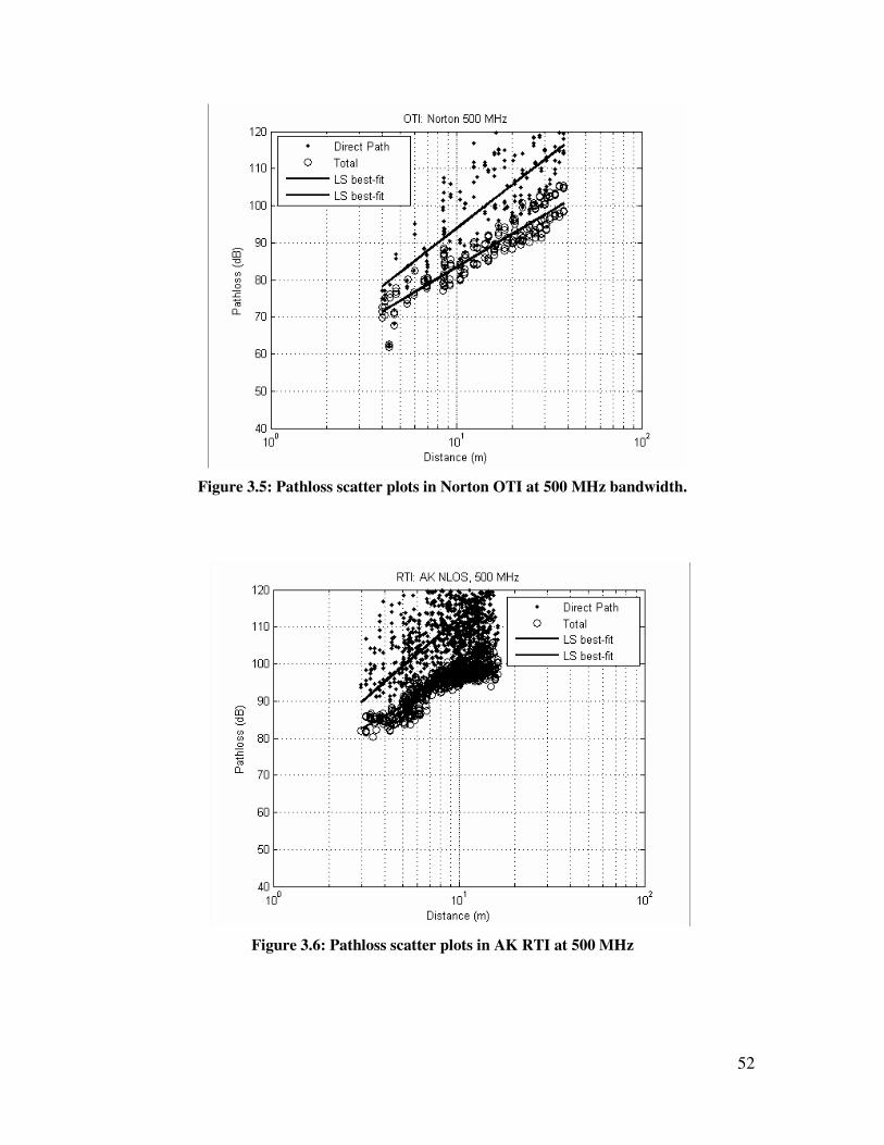
52
Figure 3.5: Pathloss scatter plots in Norton OTI at 500 MHz bandwidth.
Figure 3.6: Pathloss scatter plots in AK RTI at 500 MHz
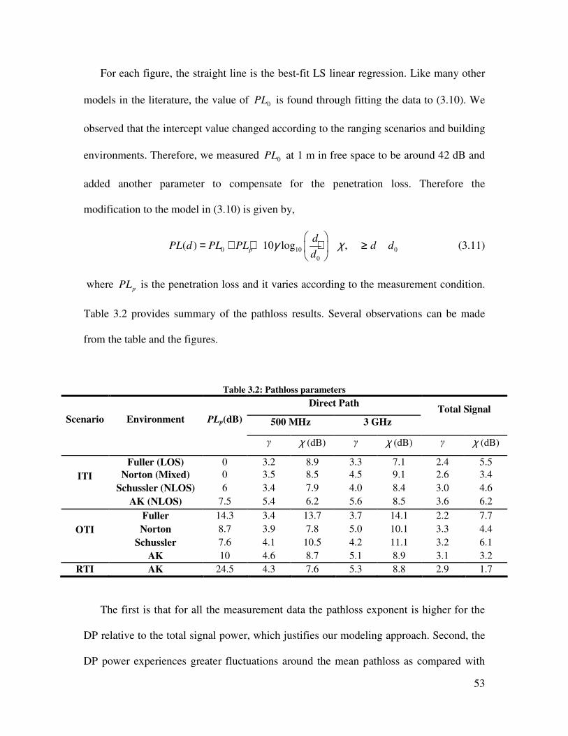
53
For each figure, the straight line is the best-fit LS linear regression. Like many other
models in the literature, the value of 0PL is found through fitting the data to (3.10). We
observed that the intercept value changed according to the ranging scenarios and building
environments. Therefore, we measured 0PL at 1 m in free space to be around 42 dB and
added another parameter to compensate for the penetration loss. Therefore the
modification to the model in (3.10) is given by,
0 10 0
0
( ) 10 log ,p
dPL d PL PL d d
dγ χ
= + + + ≥
(3.11)
where p
PL is the penetration loss and it varies according to the measurement condition.
Table 3.2 provides summary of the pathloss results. Several observations can be made
from the table and the figures.
Table 3.2: Pathloss parameters
Direct Path
500 MHz 3 GHz
Total Signal Scenario Environment PLp(dB)
γ χ (dB) γ χ (dB) γ χ (dB)
Fuller (LOS) 0 3.2 8.9 3.3 7.1 2.4 5.5
Norton (Mixed) 0 3.5 8.5 4.5 9.1 2.6 3.4
Schussler (NLOS) 6 3.4 7.9 4.0 8.4 3.0 4.6 ITI
AK (NLOS) 7.5 5.4 6.2 5.6 8.5 3.6 6.2
Fuller 14.3 3.4 13.7 3.7 14.1 2.2 7.7
Norton 8.7 3.9 7.8 5.0 10.1 3.3 4.4
Schussler 7.6 4.1 10.5 4.2 11.1 3.2 6.1
OTI
AK 10 4.6 8.7 5.1 8.9 3.1 3.2
RTI AK 24.5 4.3 7.6 5.3 8.8 2.9 1.7
The first is that for all the measurement data the pathloss exponent is higher for the
DP relative to the total signal power, which justifies our modeling approach. Second, the
DP power experiences greater fluctuations around the mean pathloss as compared with
54
the total signal counterpart. This observation makes sense because small variations on the
transmitter location affect the DP power more than the total power. Third, p
PL changes
for the different penetration scenarios. In ITI scenarios Schussler NLOS suffers 6 dB
penetration loss due to the walls compared to 7.5 in AK. Norton ITI measurements are a
mixture of LOS/NLOS because the manufacturing floor contained scattered machines
and the impact can be clearly seen on the pathloss exponent when the bandwidth
increases, hence higher attenuation. Results of OTI measurements show that Fuller and
AK exhibit the largest penetration loss mainly because the signal had to penetrate a
heavier building construction when compared with Norton and Schussler. In addition the
pathloss exponents in AK are large mainly because the measurement locations were
conducted inside a metal shop on the edge of the building and between concrete corridors
and rooms. AK in general imposes a very challenging environment for ranging because
of the building material and dense cluttering. RTI measurements experienced the largest
penetration loss and high pathloss exponent. Finally, note that the harsher the indoor
environment the higher the pathloss exponent difference when moving to a higher system
bandwidth. This is mainly due to the fact that larger system bandwidths provide better
time domain resolution at the cost of reduced power per multipath component. This
implies that the advantage of higher time-domain resolution comes at a cost of shorter
ranging coverage.
55
3.5. Modeling the Ranging Error
3.5.1. Spatial Characterization
The goal of our modeling efforts is to provide tools to simulate the spatial ranging
error behavior in indoor environments for two popular UWB system bandwidths.
Ranging errors have been modeled using different approaches. In [Ala03b] and [Den04]
they were modeled as a combination of Gaussian and exponential distributions using
Ray-Tracing (RT) simulation software and through measurements, respectively. The
latter refined the technique of the former and added an additional classification of
extreme NLOS. The main problem with this approach is that it is not based on any
system model, thereby lacking physical significance. Alternatively, our modeling
approach will focus on the behavior of errors in presence and absence of DP similar to
[Ala06].
The spatial characteristics of the ranging errors are determined by the behavior of the
biases which are random due to the unknown structure of the indoor environment and the
relative location of the user to them. Since the errors are highly dependent on the absence
or the presence of the DP, we will model it according to the error classification in Section
3.2. Further, in order to model and compare the behavior in different building
environments and scenarios, the normalized ranging error will be modeled instead, this is
given by
( )d d
d d
εψ−
= = . (3.12)
The range error experienced in an indoor environment can then be modeled by combining
the conditions in (3.6) and (3.7) through the following expression
56
( )m pd BG Xψ ψ ψ ψ= + + , (3.13)
where m
ψ is the normalized multipath error that exists in both the presence and absence
of the DP. pd
ψ is the normalized propagation delay induced error. B
ψ is the normalized
error due to DP blockage. In order to distinguish between the error behavior in LOS and
NLOS we use a Bernoulli random variable, G . That is,
0,
1,
LOSG
NLOS
=
, (3.14)
where ( ) ( )0p G p LOS= = is the probability of being in LOS and ( ) ( )1p G p NLOS= =
is the probability of being in NLOS. Similarly X is a Bernoulli random variable that
models the occurrence of DP blockage given by
1
2
0,
1,X
ζζ
=
(3.15)
where ( ) 21 ( )p X p ζ= = denotes the probability of the occurrence of blockage, while
( ) 10 ( )p X p ζ= = denote the probability of detecting a DP. Again we clarify that our
modeling approach specifically focuses on the DP and not the traditional definition of
NLOS used for communications. This means that a MT and a RP separated by a wall, for
instance, is considered NLOS, but does not necessarily mean absence of the DP. In the
remainder of the dissertation, ranging error, bias and normalized error will be used
interchangeably and it will refer to (3.13).
3.5.2. Probability of DP Blockage
The probability of a MT within the ranging coverage of a RP to experience DP
blockage depends on the system SNR, bandwidth, building environment, ranging
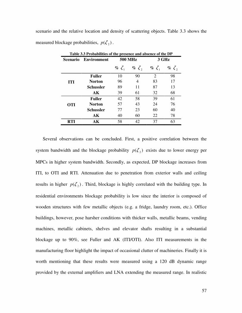
57
scenario and the relative location and density of scattering objects. Table 3.3 shows the
measured blockage probabilities, )( 2ζp .
Table 3.3 Probabilities of the presence and absence of the DP
Scenario Environment 500 MHz 3 GHz
% 1ζ % 2ζ % 1ζ % 2ζ
Fuller 10 90 2 98
Norton 96 4 83 17
Schussler 89 11 87 13 ITI
AK 39 61 32 68
Fuller 42 58 39 61
Norton 57 43 24 76
Schussler 77 23 60 40 OTI
AK 40 60 22 78
RTI AK 58 42 37 63
Several observations can be concluded. First, a positive correlation between the
system bandwidth and the blockage probability )( 2ζp exists due to lower energy per
MPCs in higher system bandwidth. Secondly, as expected, DP blockage increases from
ITI, to OTI and RTI. Attenuation due to penetration from exterior walls and ceiling
results in higher )( 2ζp . Third, blockage is highly correlated with the building type. In
residential environments blockage probability is low since the interior is composed of
wooden structures with few metallic objects (e.g. a fridge, laundry room, etc.). Office
buildings, however, pose harsher conditions with thicker walls, metallic beams, vending
machines, metallic cabinets, shelves and elevator shafts resulting in a substantial
blockage up to 90%, see Fuller and AK (ITI/OTI). Also ITI measurements in the
manufacturing floor highlight the impact of occasional clutter of machineries. Finally it is
worth mentioning that these results were measured using a 120 dB dynamic range
provided by the external amplifiers and LNA extending the measured range. In realistic
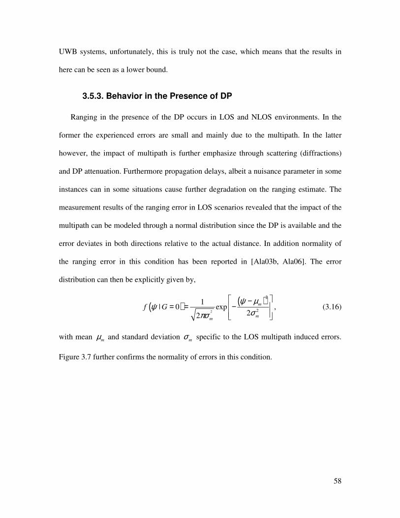
58
UWB systems, unfortunately, this is truly not the case, which means that the results in
here can be seen as a lower bound.
3.5.3. Behavior in the Presence of DP
Ranging in the presence of the DP occurs in LOS and NLOS environments. In the
former the experienced errors are small and mainly due to the multipath. In the latter
however, the impact of multipath is further emphasize through scattering (diffractions)
and DP attenuation. Furthermore propagation delays, albeit a nuisance parameter in some
instances can in some situations cause further degradation on the ranging estimate. The
measurement results of the ranging error in LOS scenarios revealed that the impact of the
multipath can be modeled through a normal distribution since the DP is available and the
error deviates in both directions relative to the actual distance. In addition normality of
the ranging error in this condition has been reported in [Ala03b, Ala06]. The error
distribution can then be explicitly given by,
( ) ( )2
2
2
1| 0 exp
22
m
mm
f Gψ µ
ψσπσ
−= = −
, (3.16)
with mean m
µ and standard deviation m
σ specific to the LOS multipath induced errors.
Figure 3.7 further confirms the normality of errors in this condition.
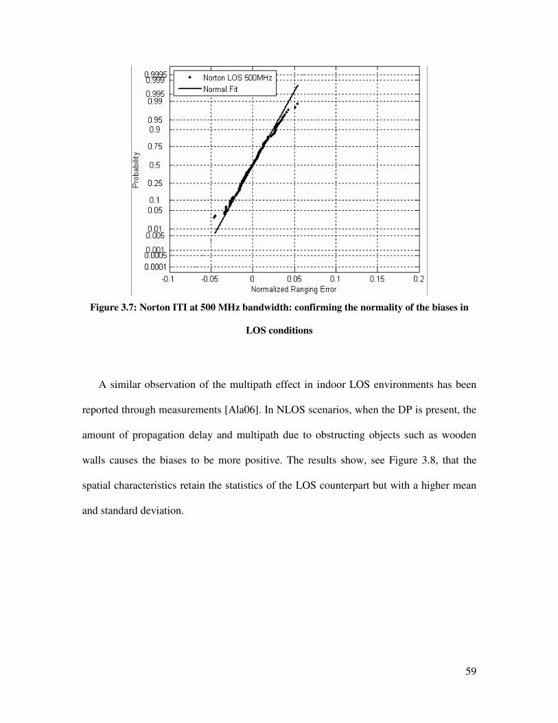
59
Figure 3.7: Norton ITI at 500 MHz bandwidth: confirming the normality of the biases in
LOS conditions
A similar observation of the multipath effect in indoor LOS environments has been
reported through measurements [Ala06]. In NLOS scenarios, when the DP is present, the
amount of propagation delay and multipath due to obstructing objects such as wooden
walls causes the biases to be more positive. The results show, see Figure 3.8, that the
spatial characteristics retain the statistics of the LOS counterpart but with a higher mean
and standard deviation.
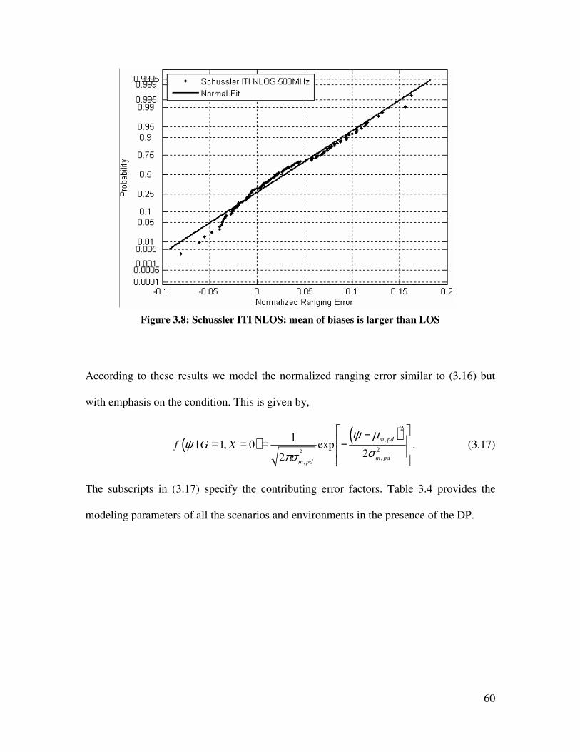
60
Figure 3.8: Schussler ITI NLOS: mean of biases is larger than LOS
According to these results we model the normalized ranging error similar to (3.16) but
with emphasis on the condition. This is given by,
( ) ( )2
2
,
2
,,
1| 1, 0 exp
22
m pd
m pdm pd
f G Xψ µ
ψσπσ
− = = = −
. (3.17)
The subscripts in (3.17) specify the contributing error factors. Table 3.4 provides the
modeling parameters of all the scenarios and environments in the presence of the DP.
61
Table 3.4: DP normal distribution modeling parameters for normalized ranging error
Scenario Environment 500 MHz 3 GHz
mµ mσ
mµ mσ
Fuller (LOS) 0 0.028 0 0.006
Norton (LOS) 0 0.022 0 0.007
,m pdµ ,m pdσ
,m pdµ ,m pdσ
Fuller (NLOS) 0.058 0.028 0.003 0.01
Schussler (NLOS) 0.029 0.047 0.014 0.016
ITI
AK (NLOS) 0.023 0.020 0.009 0.004
Fuller 0.015 0.017 0.002 0.011
Norton 0.019 0.029 0.002 0.015
Schussler 0.041 0.045 0.011 0.013 OTI
AK 0.034 0.023 0.012 0.004
RTI AK 0.029 0.041 0.012 0.012
The results show a positive correlation between the statistics of the normal distribution
with the complexity of environment and/or ranging scenario. Negative correlation can be
seen between the statistics and the system bandwidth due to reduction of multipath error
in higher bandwidths.
3.5.4. Behavior in the Absence of DP
The shadowing of the DP impacts the error behavior in several ways. First, only
positive errors occur, since the blockage induces a higher positive bias that dominates
compared to the multipath counterpart. Second, there are occasionally large positive
range errors that occur due to heavier indoor constructions such as elevator shafts,
clustering of cabinets or even metallic doors. Third, the diversity of blocking material in
indoor environments means that the spatial distribution of errors will in general exhibit a
heavier positive tail. By examining the PDF of the errors in this condition, we observed
that different subsets of the data showed varying tail behavior. The “heaviness” of the tail
depended on the ranging environment and scenario. Thus harsher blockage conditions,
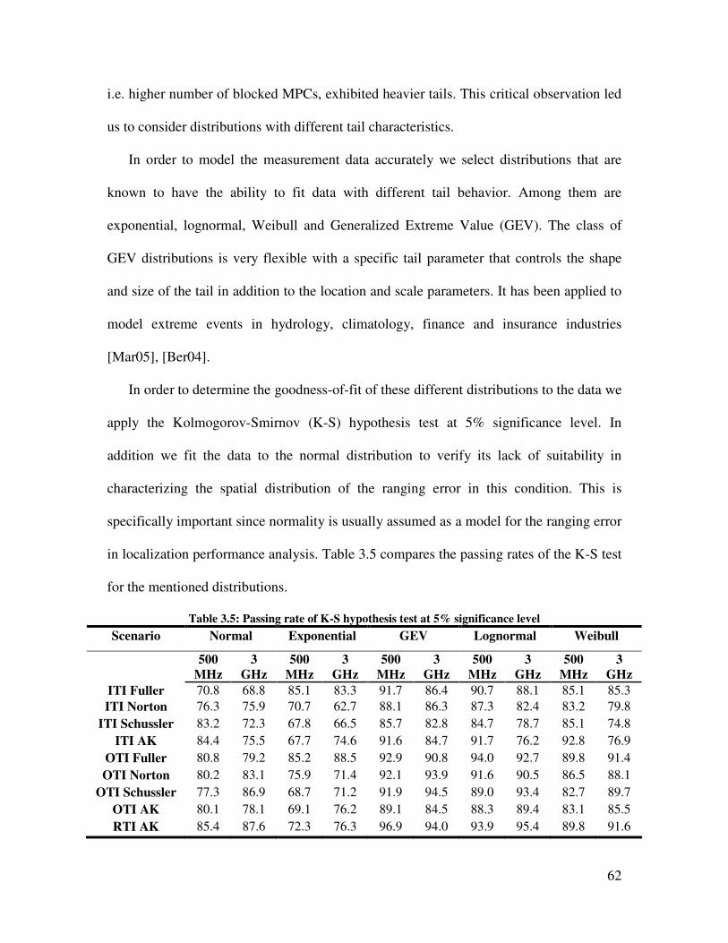
62
i.e. higher number of blocked MPCs, exhibited heavier tails. This critical observation led
us to consider distributions with different tail characteristics.
In order to model the measurement data accurately we select distributions that are
known to have the ability to fit data with different tail behavior. Among them are
exponential, lognormal, Weibull and Generalized Extreme Value (GEV). The class of
GEV distributions is very flexible with a specific tail parameter that controls the shape
and size of the tail in addition to the location and scale parameters. It has been applied to
model extreme events in hydrology, climatology, finance and insurance industries
[Mar05], [Ber04].
In order to determine the goodness-of-fit of these different distributions to the data we
apply the Kolmogorov-Smirnov (K-S) hypothesis test at 5% significance level. In
addition we fit the data to the normal distribution to verify its lack of suitability in
characterizing the spatial distribution of the ranging error in this condition. This is
specifically important since normality is usually assumed as a model for the ranging error
in localization performance analysis. Table 3.5 compares the passing rates of the K-S test
for the mentioned distributions.
Table 3.5: Passing rate of K-S hypothesis test at 5% significance level
Scenario Normal Exponential GEV Lognormal Weibull
500
MHz
3
GHz
500
MHz
3
GHz
500
MHz
3
GHz
500
MHz
3
GHz
500
MHz
3
GHz
ITI Fuller 70.8 68.8 85.1 83.3 91.7 86.4 90.7 88.1 85.1 85.3
ITI Norton 76.3 75.9 70.7 62.7 88.1 86.3 87.3 82.4 83.2 79.8
ITI Schussler 83.2 72.3 67.8 66.5 85.7 82.8 84.7 78.7 85.1 74.8
ITI AK 84.4 75.5 67.7 74.6 91.6 84.7 91.7 76.2 92.8 76.9
OTI Fuller 80.8 79.2 85.2 88.5 92.9 90.8 94.0 92.7 89.8 91.4
OTI Norton 80.2 83.1 75.9 71.4 92.1 93.9 91.6 90.5 86.5 88.1
OTI Schussler 77.3 86.9 68.7 71.2 91.9 94.5 89.0 93.4 82.7 89.7
OTI AK 80.1 78.1 69.1 76.2 89.1 84.5 88.3 89.4 83.1 85.5
RTI AK 85.4 87.6 72.3 76.3 96.9 94.0 93.9 95.4 89.8 91.6
63
The results show that both the normal and exponential distributions are not valid models
for the ranging error in the absence of the DP because they are consistently poor in
passing the K-S test, below 80% for most data sets. Similarly for the Weibull distribution
most of the passing rate is below 90%. Comparing these results to GEV and lognormal, it
is possible to see that their passing rate is above 90% for most of the data sets. Only in
ITI Schussler is their performance similar to the Weibull and normal distributions; which
is mainly due to the lightness of the tail. In addition, GEV distribution passing rates are
close to the lognormal. For some data sets, the difference between their passing rates is
less than 2%. As a result these two distributions are the best candidates for modeling the
tail behavior of errors in the absence of the DP. The GEV distribution models the tail
behavior with three degrees of freedom, compared with two in the lognormal distribution,
providing enhanced flexibility in capturing the error statistics in a variety of
circumstances. It is defined as
ξξ
σµξ
σµξ
σσµξ
11/1
11exp1
),,;(
−−−
−+
−+−= xxxf (3.18)
for 0/)(1 >−+ σµξ x ; where µ , σ and ξ are the location, scale and shape parameters,
respectively. GEV combines three simpler distributions in the form given in (3.18). The
value of the shape parameter specifies the type of the distribution. Type I, also known as
Gumbel, corresponds to 0=ξ . Type II, Frechet, corresponds to 0>ξ . Type III, Weibull,
corresponds to 0<ξ . The Gumbel and Weibull in the GEV sense correspond to the
mirror images of the usual distributions [Cas88]. The normalized error data in all the
measurement sets in the absence of the DP fit the Frechet type of the GEV. Although this
is a candidate fit to our data we choose lognormal instead for the following reasons. First
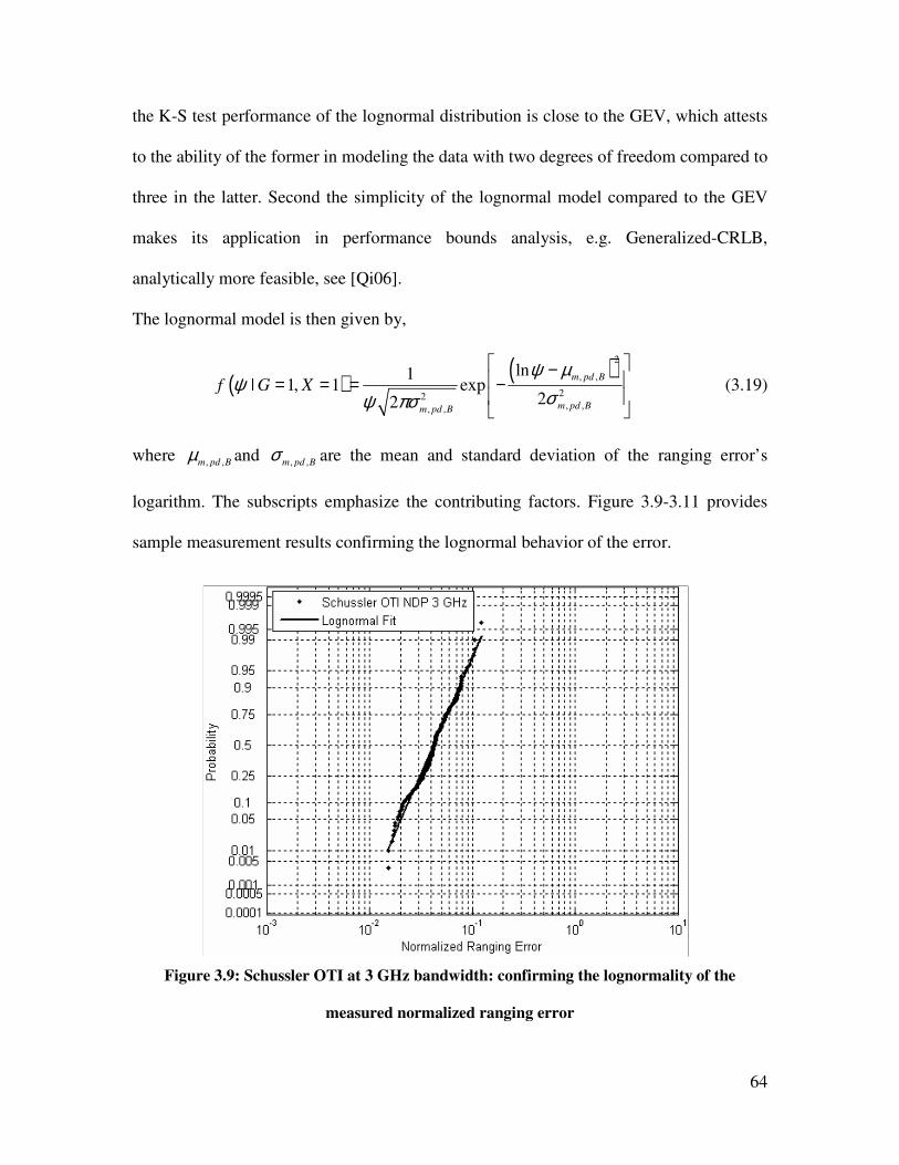
64
the K-S test performance of the lognormal distribution is close to the GEV, which attests
to the ability of the former in modeling the data with two degrees of freedom compared to
three in the latter. Second the simplicity of the lognormal model compared to the GEV
makes its application in performance bounds analysis, e.g. Generalized-CRLB,
analytically more feasible, see [Qi06].
The lognormal model is then given by,
( ) ( )2
, ,
22, ,, ,
ln1| 1, 1 exp
22
m pd B
m pd Bm pd B
f G Xψ µ
ψσψ πσ
− = = = −
(3.19)
where , ,m pd Bµ and , ,m pd B
σ are the mean and standard deviation of the ranging error’s
logarithm. The subscripts emphasize the contributing factors. Figure 3.9-3.11 provides
sample measurement results confirming the lognormal behavior of the error.
Figure 3.9: Schussler OTI at 3 GHz bandwidth: confirming the lognormality of the
measured normalized ranging error
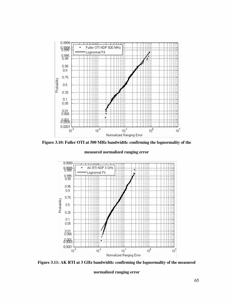
65
Figure 3.10: Fuller OTI at 500 MHz bandwidth: confirming the lognormality of the
measured normalized ranging error
Figure 3.11: AK RTI at 3 GHz bandwidth: confirming the lognormality of the measured
normalized ranging error
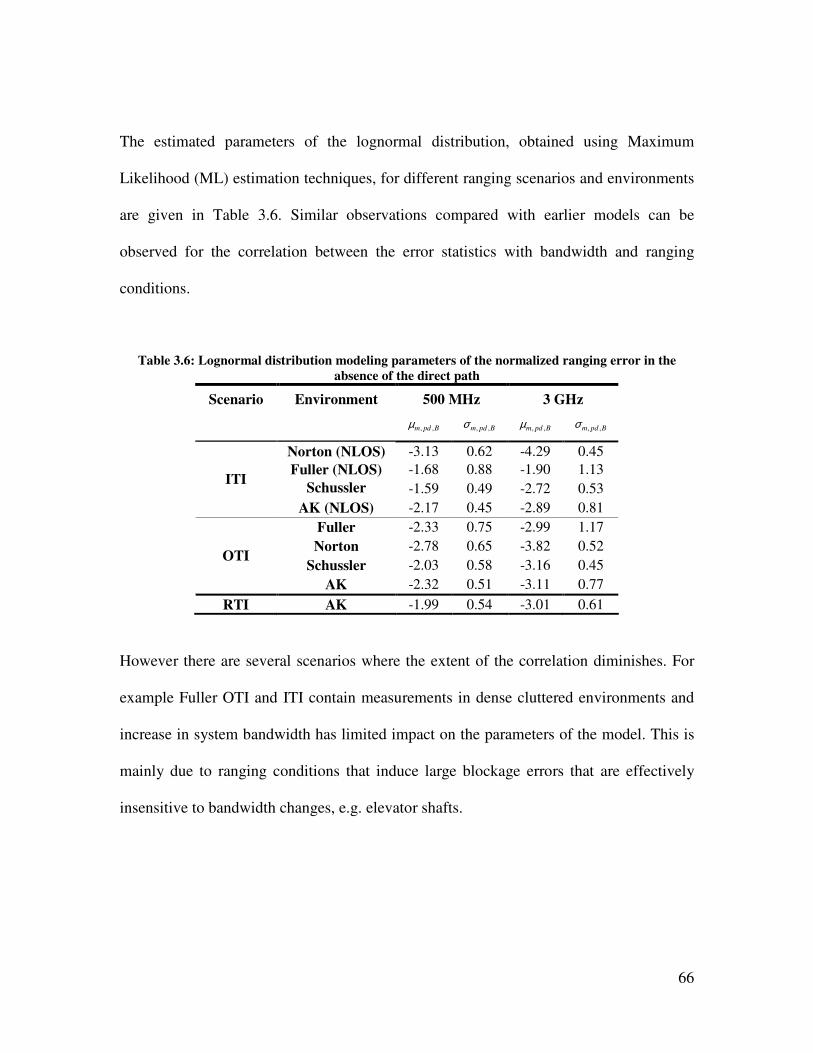
66
The estimated parameters of the lognormal distribution, obtained using Maximum
Likelihood (ML) estimation techniques, for different ranging scenarios and environments
are given in Table 3.6. Similar observations compared with earlier models can be
observed for the correlation between the error statistics with bandwidth and ranging
conditions.
Table 3.6: Lognormal distribution modeling parameters of the normalized ranging error in the
absence of the direct path
Scenario Environment 500 MHz 3 GHz
, ,m pd Bµ , ,m pd Bσ
, ,m pd Bµ , ,m pd Bσ
Norton (NLOS) -3.13 0.62 -4.29 0.45
Fuller (NLOS) -1.68 0.88 -1.90 1.13
Schussler
(NLOS) -1.59 0.49 -2.72 0.53
ITI
AK (NLOS) -2.17 0.45 -2.89 0.81
Fuller -2.33 0.75 -2.99 1.17
Norton -2.78 0.65 -3.82 0.52
Schussler -2.03 0.58 -3.16 0.45 OTI
AK -2.32 0.51 -3.11 0.77
RTI AK -1.99 0.54 -3.01 0.61
However there are several scenarios where the extent of the correlation diminishes. For
example Fuller OTI and ITI contain measurements in dense cluttered environments and
increase in system bandwidth has limited impact on the parameters of the model. This is
mainly due to ranging conditions that induce large blockage errors that are effectively
insensitive to bandwidth changes, e.g. elevator shafts.
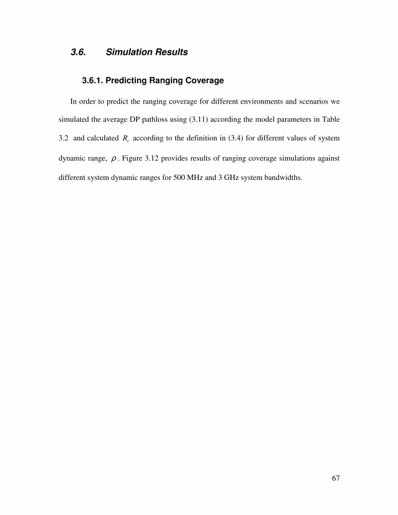
67
3.6. Simulation Results
3.6.1. Predicting Ranging Coverage
In order to predict the ranging coverage for different environments and scenarios we
simulated the average DP pathloss using (3.11) according the model parameters in Table
3.2 and calculated c
R according to the definition in (3.4) for different values of system
dynamic range, ρ . Figure 3.12 provides results of ranging coverage simulations against
different system dynamic ranges for 500 MHz and 3 GHz system bandwidths.
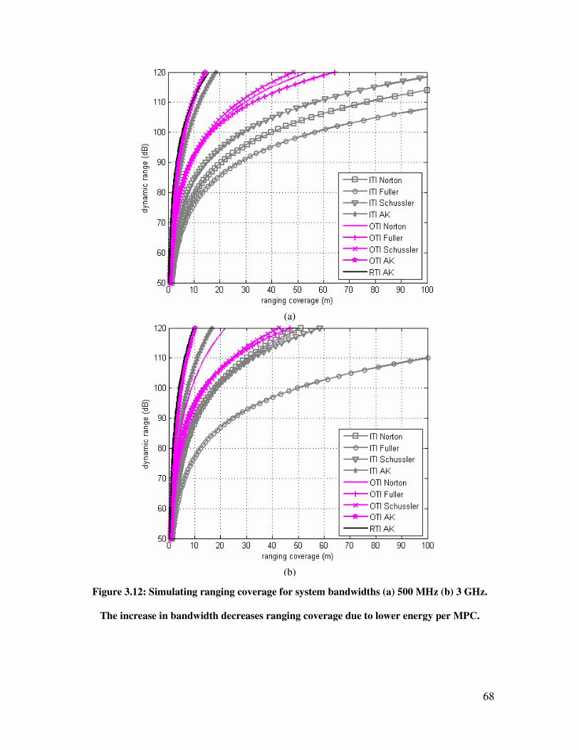
68
Figure 3.12: Simulating ranging coverage for system bandwidths (a) 500 MHz (b) 3 GHz.
The increase in bandwidth decreases ranging coverage due to lower energy per MPC.
(a)
(b)

69
As reflected in the measurement results, RTI faces the toughest constraint for ranging.
The simulation reveals that for a dynamic range of around 100 dB and 500 MHz
bandwidth, ranging coverage for AK RTI and OTI is less than 10 meters. For other OTI
environments it is around 15 m; while ITI varies between 25-60 m depending on the LOS
or NLOS conditions. Another observation from the simulation results is that the change
in system bandwidth reduces the coverage substantially. This is less the case for pure
LOS scenarios where the coverage is almost the same for both bandwidths, see ITI Fuller.
The other ITI environments, however, are mixed LOS/NLOS for Norton and pure NLOS
for Schussler and AK and that can be clearly observed in the change of their coverage
between the bandwidths.
3.6.2. Ranging Error Simulation
The models presented in section 3.5, provide a very simple, yet realistic and flexible
approach to statistically characterizing ranging errors experienced in typical indoor
environments. The model parameters G and X provide control over the LOS/NLOS and
the presence/absence of the DP conditions, respectively. The model distribution
parameters then provide control over the error experienced in each condition. In order to
further validate our modeling approach we simulate the normalized ranging error
according to the models in section 3.5 and compare them with the measurements. For
each ranging condition and scenario we run Monte Carlo simulations with 10,000
normalized range error samples. We focus on NLOS conditions since performance in
LOS is intuitive and has been addressed sufficiently in the literature. Therefore we set
( )1 1p G = = and for each sample, we run a Bernoulli trial with ( ) ( )21p X p ζ= = , from
Table 3.3, where the outcome determines the distribution, (3.17) or (3.19). The simulated
70
samples are stacked in a vector and their CDF is compared to the measurement data set in
that specific scenario and environment. Figure 3.13 and 3.14 provide several examples
comparing the results of simulation to the measurements.

71
Figure 3.13: CDF of normalized ranging error: simulation vs. measurements. (a) Schussler
OTI (b) AK RTI
(a)
(b)
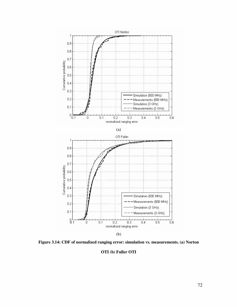
72
Figure 3.14: CDF of normalized ranging error: simulation vs. measurements. (a) Norton
OTI (b) Fuller OTI
(a)
(b)
73
The models show close agreement with the measurements. This is mainly because the
model has the ability to statistically describe the error in 1ζ and 2ζ independently. This
approach provides flexibility in modeling the factors contributing to the error, which will
be different depending on the ranging situation. For instance, if several MTs are scattered
in an indoor environment and RPs are fixed in different locations in and surrounding the
building then the ranging error PDF of all the ranging estimates can be described
according to these models. The distribution will vary from heavy-tailed to normally
distributed as the range conditions change from extreme NLOS to LOS.
3.7. Conclusion
In this chapter we have described a comprehensive UWB measurement and modeling
campaign that was aimed at characterizing the spatial behavior of indoor TOA-based
ranging. Spatial characterization involved analyzing and modeling the coverage and
accuracy of ranging in indoor environments. The measurement involved four different
building environments: residential, traditional office, modern office and manufacturing
floor and three different ranging scenarios ITI, OTI and RTI. We showed that ranging
coverage is inversely related to the bandwidth of the system and the harshness of the
ranging scenario and environment. In addition, ranging error can be modeled as normal
or lognormal in the presence or the absence of the DP, respectively. Furthermore, the
modeling parameters are affected by the ranging scenario, environment and system
bandwidth.
The modeling results in this dissertation provide an experimental analysis of the
physical constraints imposed by the dense cluttered indoor environments on TOA-based

74
UWB ranging. In addition the models should help researchers obtain localization bounds
specific to indoor environments, which are important in assessing and evaluating the
limitations facing different localization algorithms.
75
Chapter 4 Cooperative Localization Bounds
for Indoor UWB WSNs
4.1. Introduction
As we have seen from chapter 3, TOA-based ranging in indoor environments is
constrained by ranging coverage and error. In addition the indoor boiling environment
can cause limitation to OTI and RTI ranging due to signal penetration through the wall
and roof, respectively. This can be a major challenge for firefighter or military
applications. In these indoor cooperative localization applications, a small number (M) of
sensors called anchors are deployed outside surrounding a building where they obtain
their location information via GPS or are pre-programmed during setup. The N un-
localized sensor nodes are then deployed inside the building, e.g. fire fighters or soldiers
entering a hostile building, who with the help of the M anchors attempt to obtain their
own location information. In traditional approaches, such as geometrical triangulation
techniques, the exterior anchor nodes usually fail to cover a large building which makes
localization ineffective. In addition, the problems of indoor multipath and NLOS channel
conditions further degrade the range estimates yielding unreliable localization
performance [Pah02]. Implementation of the cooperative localization approach, as seen in
Figure 4.1, extends the coverage of the outside anchors to the inside nodes and has the
ability to enhance localization accuracy through the availability of more range
measurements between the sensor nodes.
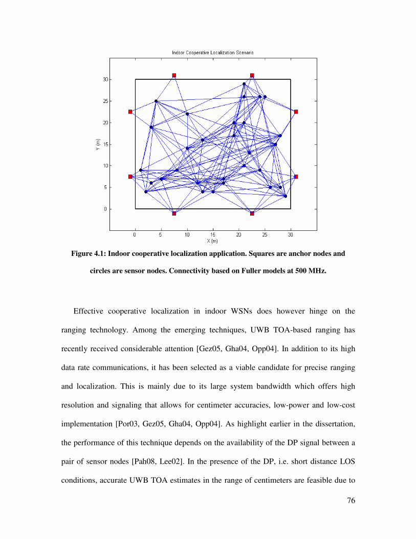
76
Figure 4.1: Indoor cooperative localization application. Squares are anchor nodes and
circles are sensor nodes. Connectivity based on Fuller models at 500 MHz.
Effective cooperative localization in indoor WSNs does however hinge on the
ranging technology. Among the emerging techniques, UWB TOA-based ranging has
recently received considerable attention [Gez05, Gha04, Opp04]. In addition to its high
data rate communications, it has been selected as a viable candidate for precise ranging
and localization. This is mainly due to its large system bandwidth which offers high
resolution and signaling that allows for centimeter accuracies, low-power and low-cost
implementation [Por03, Gez05, Gha04, Opp04]. As highlight earlier in the dissertation,
the performance of this technique depends on the availability of the DP signal between a
pair of sensor nodes [Pah08, Lee02]. In the presence of the DP, i.e. short distance LOS
conditions, accurate UWB TOA estimates in the range of centimeters are feasible due to
77
the high time-domain resolution [Fon02, Chu03, Ala06, Tar06]. The challenge, however,
is UWB ranging in indoor NLOS conditions which can be characterized as dense
multipath environments [Lee02, Pah98]. In these conditions the DP between a pair of
nodes can be blocked with high probability, substantially degrading the range and
localization accuracy. Therefore, there is a need to analyze the impact of these channel
limitations on the performance of cooperative localization in indoor WSNs.
Evaluation of localization bounds in multi-hop WSNs have been examined
extensively [Lar04, Sav05, Cha06], where the focus has been on analyzing the impact of
network parameters such as the number of anchors, node density and deployment
topology affecting localization accuracy. These localization bounds, however, have been
analyzed with unbiased ranging assumptions between sensor nodes. In [Koo98, Bot04]
the impact of biased TOA range measurements on the accuracy of location estimates is
investigated for cellular network applications. Their approach assumes NLOS induced
errors as small perturbations, which clearly is not the case in indoor environments. A
comprehensive treatment of the impact of biases on the wireless geolocation accuracy in
NLOS environments is reported in [Qi06]. Recently, position error bounds for dense
cluttered indoor environments have been reported in [Jou06a, Jou06b] where the impact
of the channel condition on the localization error is further verified in traditional
localization.
In this chapter, based on empirical UWB TOA-based OTI and ITI ranging models in
different indoor building environments reported in [Als07a, Als07b, Als08a] and
presented in chapter 3, we extend the analysis of localization bounds in NLOS
environments [Qi06] to cooperative localization in indoor multi-hop WSNs. We focus on
78
firefighter or military operation applications where we analyze the fundamental
limitations imposed by the indoor dense cluttered environment. Specifically we analyze
the impact of the channel modeling parameters such as ranging coverage, statistics of the
ranging error, probability of NLOS and probability of DP blockage on localization
accuracy. This modeling framework is necessary since OTI channel behavior affects
anchor-node range estimation while ITI affects the node-node ranges. We first show that
for the aforementioned indoor localization application, where traditional multi-lateration
fails, cooperative localization, besides providing localization for the entire network, has
the potential to further enhance the accuracy. We then evaluate the factors affecting
localization accuracy, namely network and channel modeling parameters in different
indoor environments: residential, manufacturing floor, traditional and modern office
buildings. Indoor channel ranging model-specific cooperative localization bounds in
WSNs are novel and provide comprehensive insight into the fundamental limitations
facing indoor UWB TOA-based localization in both traditional and sensor networks.
The organization of this chapter is as follows. In section 4.2 we review the classification
of UWB TOA-based ranging in indoor environments. In section 4.3, we present the
problem formulation. In section 4.4 we derive the Generalized Cramer-Rao Lower Bound
(G-CRLB) for cooperative localization in indoor multi-hop WSNs. In section 4.5 we
provide results of simulation which highlight the network and ranging channel modeling
parameters that affect the localization accuracy. Finally, we conclude the chapter in
section 4.6.
79
4.2. UWB TOA-based Ranging Overview
Before proceeding with derivation of the theoretic limits of cooperative localization
in indoor environments, it is necessary to review the behavior of UWB TOA-based
ranging coverage and errors for the purpose of clarity. In addition to ranging coverage,
localization bounds in indoor multipath channels are further constrained by the statistics
of ranging error. The behavior of ranging error between a pair of nodes depends on the
availability of the DP and in the case of its absence, on the statistics of the blockage. As
seen in the earlier chapter the ranging error experienced in an indoor environment can
then be modeled by combining the conditions in (3.6) and (3.7) through the following
expression,
( ) ( )( )m pd Bb G b X bε ω ω= + ⋅ + ⋅ , (4.1)
In order to facilitate the notations for the G-CRLB derivations we assign specific
variables for each of the channel conditions in (4.1) that is,
, 0, 0
, 1, 0
, 1, 1
G X
G X
G X
λε η
β
= == = = = =
. (4.2)
The probability density functions (PDFs) of these conditions, ( )f λλ , ( )f ηη and ( )f ββ ,
have been experimentally obtained through comprehensive UWB channel measurements
for the different ranging environments and scenarios [Als07b, Als08a] and their distance
normalized distribution were introduced in chapter 3. Figure 4.2 further illustrates the
different ranging conditions that are possible in a given indoor WSN.
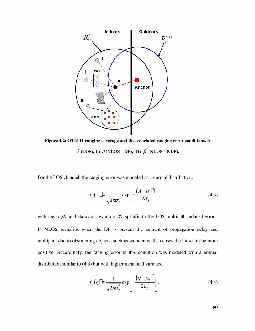
80
Figure 4.2: OTI/ITI ranging coverage and the associated ranging error conditions. I:
λ (LOS), II: η (NLOS – DP), III: β (NLOS – NDP).
For the LOS channel, the ranging error was modeled as a normal distribution,
( ) ( )2
2
2
1exp
22f
λ
λλ
λ µλ
σπσ
−= −
λ
, (4.3)
with mean λµ and standard deviation λσ specific to the LOS multipath induced errors.
In NLOS scenarios when the DP is present the amount of propagation delay and
multipath due to obstructing objects, such as wooden walls, causes the biases to be more
positive. Accordingly, the ranging error in this condition was modeled with a normal
distribution similar to (4.3) but with higher mean and variance,
( ) ( )2
2
2
1exp
22f
η
ηη
η µη
σπσ
− = −
η. (4.4)
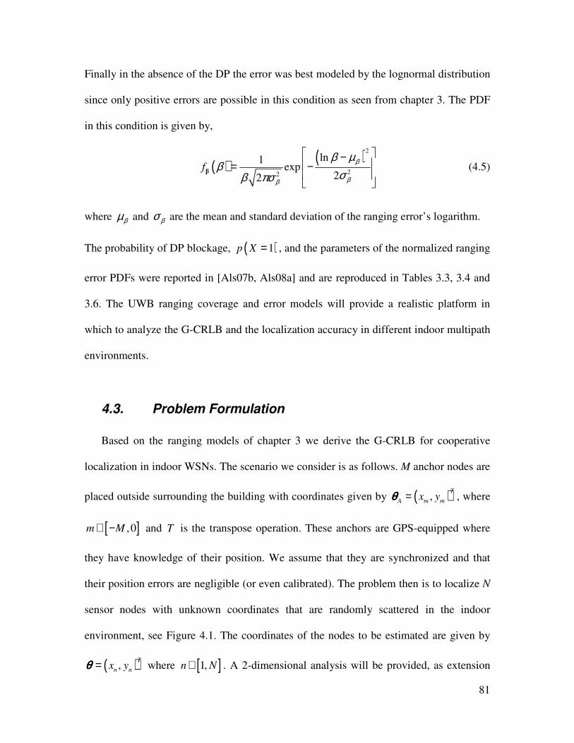
81
Finally in the absence of the DP the error was best modeled by the lognormal distribution
since only positive errors are possible in this condition as seen from chapter 3. The PDF
in this condition is given by,
( ) ( )2
22
ln1exp
22f
β
ββ
β µβ
σβ πσ
− = −
β (4.5)
where βµ and βσ are the mean and standard deviation of the ranging error’s logarithm.
The probability of DP blockage, ( )1p X = , and the parameters of the normalized ranging
error PDFs were reported in [Als07b, Als08a] and are reproduced in Tables 3.3, 3.4 and
3.6. The UWB ranging coverage and error models will provide a realistic platform in
which to analyze the G-CRLB and the localization accuracy in different indoor multipath
environments.
4.3. Problem Formulation
Based on the ranging models of chapter 3 we derive the G-CRLB for cooperative
localization in indoor WSNs. The scenario we consider is as follows. M anchor nodes are
placed outside surrounding the building with coordinates given by ( ),T
A m mx y=θθθθ , where
[ ],0m M∈ − and T is the transpose operation. These anchors are GPS-equipped where
they have knowledge of their position. We assume that they are synchronized and that
their position errors are negligible (or even calibrated). The problem then is to localize N
sensor nodes with unknown coordinates that are randomly scattered in the indoor
environment, see Figure 4.1. The coordinates of the nodes to be estimated are given by
( ),T
n nx y=θθθθ where [ ]1,n N∈ . A 2-dimensional analysis will be provided, as extension
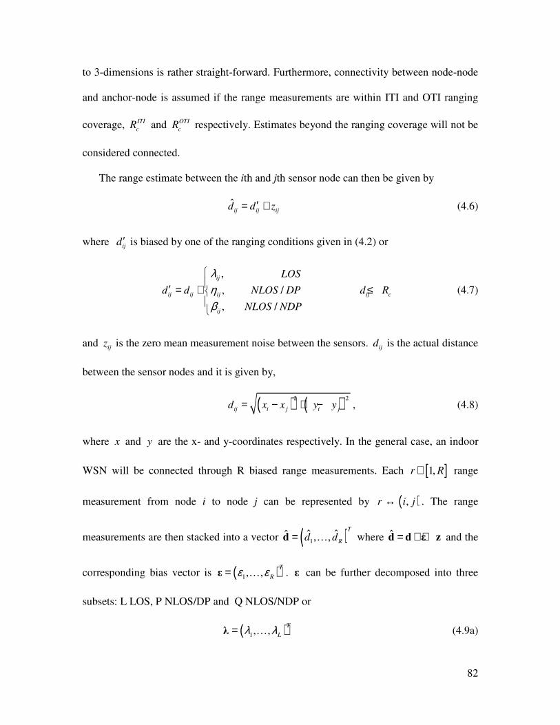
82
to 3-dimensions is rather straight-forward. Furthermore, connectivity between node-node
and anchor-node is assumed if the range measurements are within ITI and OTI ranging
coverage, ITI
cR and OTI
cR respectively. Estimates beyond the ranging coverage will not be
considered connected.
The range estimate between the ith and jth sensor node can then be given by
ˆij ij ijd d z′= + (4.6)
where ij
d ′ is biased by one of the ranging conditions given in (4.2) or
,
, /
, /
ij
ij ij ij ij c
ij
LOS
d d NLOS DP d R
NLOS NDP
ληβ
′ = + ≤
(4.7)
and ij
z is the zero mean measurement noise between the sensors. ij
d is the actual distance
between the sensor nodes and it is given by,
( ) ( )2 2
ij i j i jd x x y y= − + − , (4.8)
where x and y are the x- and y-coordinates respectively. In the general case, an indoor
WSN will be connected through R biased range measurements. Each [ ]1,r R∈ range
measurement from node i to node j can be represented by ( ),r i j↔ . The range
measurements are then stacked into a vector ( )1ˆ ˆˆ , ,
T
Rd d=d … where ˆ = + +d d ε z and the
corresponding bias vector is ( )1, ,T
Rε ε=ε … . ε can be further decomposed into three
subsets: L LOS, P NLOS/DP and Q NLOS/NDP or
( )1, ,T
Lλ λ=λ … (4.9a)
83
( )1, ,T
Pη η=η … (4.9b)
( )1, ,T
Qβ β=β … (4.9c)
where R L P Q= + + . We further assume that it is possible to distinguish between these
different ranging conditions through NLOS and DP blockage identification algorithms
[Hei07, Guv07]. Note that even in LOS our modeling assumption maintains the existence
of bias due to multipath. This is usually neglected in LOS analysis, since single-path
propagation is assumed [Qi06]. The statistics of the multipath biases, obtained from
measurements, are incorporated into the analysis to provide a realistic evaluation of the
problem.
4.4. The Generalized Cramer-Rao Lower Bound
The unknown vector of parameters to be estimated is then obtained by combining the
coordinates of the unknown nodes’ positions with the bias vector, or
( )1 1 1 1 1, , , , , , , , , , ,T
N N L P Qx y x y λ λ η η β β= … … … …θθθθ . (4.10)
The CRLB provides a lower bound on the variance of any unbiased estimate of the
unknown parameters [Van68]. In the case the estimates are biased it is possible to obtain
the G-CRLB given that the statistics of the biases are available a priori [Qi06, Van68].
The empirical PDFs of λ , η and β or ( )f λλ , ( )f ηη and ( )f ββ respectively were
introduced in chapter 3 and their distance-normalized parameters are presented in Tables
3.4 and 3.6.
The G-CRLB is then given by [Van68],
84
( )( ) 1ˆ ˆT
E− − − ≥
Jθ θ θ θθ θ θ θθ θ θ θθ θ θ θ , (4.11)
where [ ]E ⋅ is the expectation operation and J is the information matrix that consists of
two parts,
= +J J Jθθθθ P . (4.12)
Jθθθθ is the Fisher information matrix (FIM) which represents the data and JP represents
the a priori information that reflects the statistics of the biases. Specifically, the data FIM
can be obtained by evaluating,
( ) ( )ˆ ˆln | ln |
T
E f f ∂ ∂ = ⋅ ∂ ∂
Jθ θθ θθ θθ θ θ θθ θθ θθ θθ θθ θθ θθ θ
d d (4.13)
where ( )ˆ |f θθθθd is the joint PDF of the range measurement vector ( )ˆ ˆˆ ,T
1 Rd , d…d =
conditioned on θθθθ . Since the measurement noise is usually assumed zero mean Gaussian,
the joint PDF can be given by,
( ) ( ) ( )1ˆ ˆ ˆ| exp2
T
f ′ ′∝ − − −
Λθθθθd d d d d (4.14)
where Λ is the inverse of the measurements’ covariance matrix or
( )( )1 ˆ ˆT
E− ′ ′= − −
Λ d d d d and ′d is the biased vector of the range measurements.
Assuming that the measurements are uncorrelated, Λ is then diagonal with the elements
given by ( )1
2 2, ,Rz z
diag σ σ− −=Λ … . Since ( )ˆ |f θθθθd is a function of ′d which is in turn a
function of θθθθ , Jθθθθ can be obtained by application of the chain rule or,
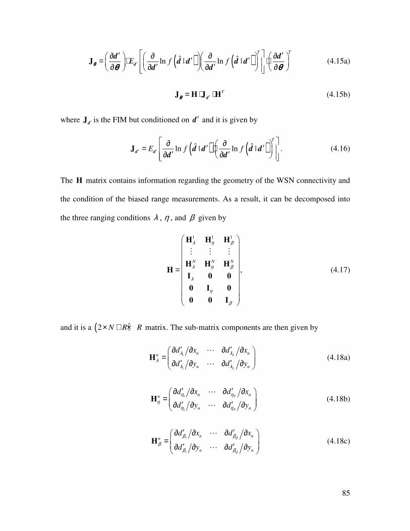
85
( ) ( )ˆ ˆln | ln |
T T
E f f′
′ ′∂ ∂ ∂ ∂ ′ ′= ⋅ ⋅ ′ ′∂ ∂ ∂ ∂ Jθθθθ θ θθ θθ θθ θd
d dd d d d
d d (4.15a)
T
′= ⋅ ⋅J H J Hθθθθ d (4.15b)
where ′Jd is the FIM but conditioned on ′d and it is given by
( ) ( )ˆ ˆln | ln |
T
E f f′ ′
∂ ∂ ′ ′= ⋅ ′ ′∂ ∂ Jd d d d d d
d d. (4.16)
The H matrix contains information regarding the geometry of the WSN connectivity and
the condition of the biased range measurements. As a result, it can be decomposed into
the three ranging conditions λ , η , and β given by
1 1 1
N N N
λ η β
λ η β
λ
η
β
=
H H H
H H HH
I 0 0
0 I 0
0 0 I
⋮ ⋮ ⋮
, (4.17)
and it is a ( )2 N R R× + × matrix. The sub-matrix components are then given by
1
1
L
L
n nn
n n
d x d x
d y d y
λ λλ
λ λ
′ ′∂ ∂ ∂ ∂ = ′ ′∂ ∂ ∂ ∂
H⋯
⋯ (4.18a)
1
1
P
P
n nn
n n
d x d x
d y d y
η ηη
η η
′ ′∂ ∂ ∂ ∂ = ′ ′∂ ∂ ∂ ∂
H⋯
⋯ (4.18b)
1
1
Q
Q
n nn
n n
d x d x
d y d y
β β
ββ β
′ ′∂ ∂ ∂ ∂ = ′ ′∂ ∂ ∂ ∂
H⋯
⋯ (4.18c)

86
for [ ]1,n N∈ and their respective dimensions are ( )2 L× , ( )2 P× and ( )2 Q× . λI , ηI ,
and βI are the identity matrices of order L, P and Q, respectively. Elements of (4.18) will
be non-zero when a range measurement is connected to node ( ),T
n nx y and zero
otherwise. For example if node 1 with coordinates ( )1 1,T
x y is connected to node 2 with
coordinates ( )2 2,T
x y by the LOS range ( ) ( )1
2 2
1 2 1 2 1d x x y yλ λ′ = − + − + then the
respective element in (4.18a) is
( ) ( ) ( )
( ) ( ) ( )1
1
2 2
1 2 1 2 1 21
2 21
1 2 1 2 1 2
x x x x y yd x
d yy y x x y y
λ
λ
′ − − + −∂ ∂ = ′∂ ∂ − − + −
. (4.19)
Similarly, ′Jd can be decomposed according to the ranging conditions where
λ
η
β
′
=
Λ 0 0
J 0 Λ 0
0 0 Λ
d (4.20)
is an R R× matrix. Specifically, ( )1
2 2,Lz z
diagλ σ σ− −=Λ … , ( )1
2 2,Pz z
diagη σ σ− −=Λ … and
( )1
2 2,Qz z
diagβ σ σ− −=Λ … . In this dissertation our focus is on analyzing the impact of the
biases due to multipath and DP blockage and in reality, the measurement noise time
variations in these different ranging conditions might not differ significantly for a high
system dynamic range [Alj04]. As a result we will assume equal noise variance, that is
λ η β= =Λ Λ Λ . Jθθθθ can then be obtained by substituting (4.17) and (4.20) into (4.15b) or,
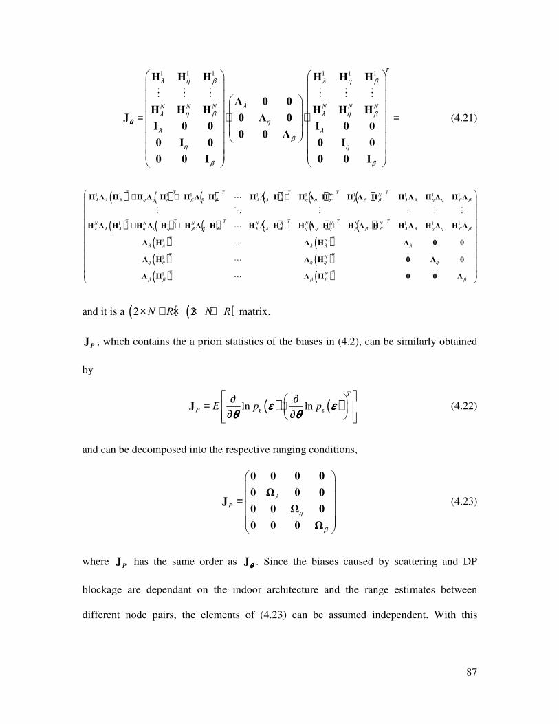
87
1 1 1 1 1 1T
N N N N N N
λ η β λ η β
λλ η β λ η β
ηλ λ
βη η
β β
= ⋅ ⋅ =
H H H H H H
Λ 0 0H H H H H H
J 0 Λ 0I 0 0 I 0 0
0 0 Λ0 I 0 0 I 0
0 0 I 0 0 I
⋮ ⋮ ⋮ ⋮ ⋮ ⋮
θθθθ (4.21)
( ) ( ) ( ) ( ) ( ) ( )
( ) ( ) ( ) ( ) ( ) ( )( ) ( )( ) ( )( ) ( )
1 1 1 1 1 1 1 1 1 1 1 1
1 1 1 1 1 1
1
1
1
T T T T T TN N N
T T T T T TN N N N N N N N N
T TN
T TN
TN
λ λ λ η η η β β β λ λ λ η η η β β β λ λ η η β β
λ λ λ η η η β β β λ λ λ η η η β β β λ λ η η β β
λ λ λ λ λ
η η η η η
β β β β
+ + + +
+ + + +
H Λ H H Λ H H Λ H H Λ H H Λ H H Λ H H Λ H Λ H Λ
H Λ H H Λ H H Λ H H Λ H H Λ H H Λ H H Λ H Λ H Λ
Λ H Λ H Λ 0 0
Λ H Λ H 0 Λ 0
Λ H Λ H
⋯
⋮ ⋱ ⋮ ⋮ ⋮ ⋮
⋯
⋯
⋯
⋯T
β
0 0 Λ
and it is a ( ) ( )2 2N R N R× + × × + matrix.
JP , which contains the a priori statistics of the biases in (4.2), can be similarly obtained
by
( ) ( )ln ln
T
E p p ∂ ∂ = ⋅ ∂ ∂
ε εJ ε εε εε εε εθ θθ θθ θθ θP (4.22)
and can be decomposed into the respective ranging conditions,
λ
η
β
=
0 0 0 0
0 Ω 0 0J
0 0 Ω 0
0 0 0 Ω
P (4.23)
where JP has the same order as Jθθθθ . Since the biases caused by scattering and DP
blockage are dependant on the indoor architecture and the range estimates between
different node pairs, the elements of (4.23) can be assumed independent. With this
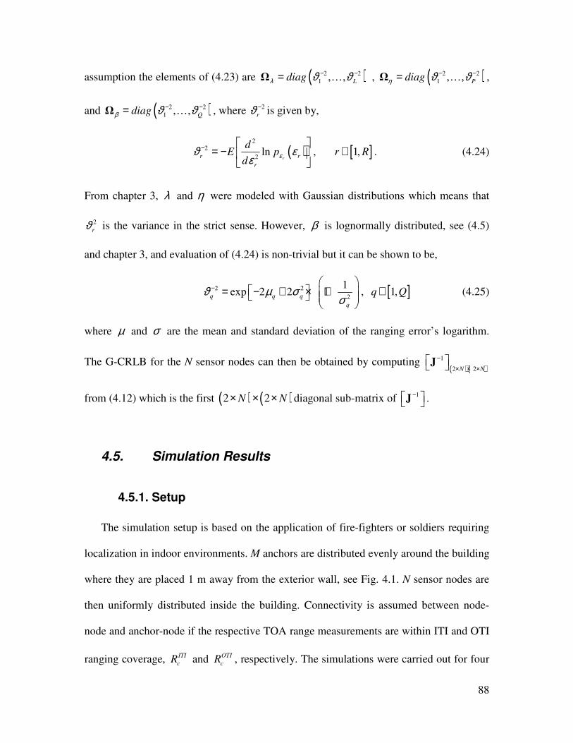
88
assumption the elements of (4.23) are ( )2 2
1 , ,L
diagλ ϑ ϑ− −=Ω … , ( )2 2
1 , ,P
diagη ϑ ϑ− −=Ω … ,
and ( )2 2
1 , ,Q
diagβ ϑ ϑ− −=Ω … , where 2
rϑ− is given by,
( )2
2
2ln
rr r
r
dE p
dεϑ ε
ε−
= −
, [ ]1,r R∈ . (4.24)
From chapter 3, λ and η were modeled with Gaussian distributions which means that
2
rϑ is the variance in the strict sense. However, β is lognormally distributed, see (4.5)
and chapter 3, and evaluation of (4.24) is non-trivial but it can be shown to be,
2 2
2
1exp 2 2 1q q q
q
ϑ µ σσ
−
= − + × +
, [ ]1,q Q∈ (4.25)
where µ and σ are the mean and standard deviation of the ranging error’s logarithm.
The G-CRLB for the N sensor nodes can then be obtained by computing ( ) ( )
1
2 2N N
−
× × × J
from (4.12) which is the first ( ) ( )2 2N N× × × diagonal sub-matrix of 1− J .
4.5. Simulation Results
4.5.1. Setup
The simulation setup is based on the application of fire-fighters or soldiers requiring
localization in indoor environments. M anchors are distributed evenly around the building
where they are placed 1 m away from the exterior wall, see Fig. 4.1. N sensor nodes are
then uniformly distributed inside the building. Connectivity is assumed between node-
node and anchor-node if the respective TOA range measurements are within ITI and OTI
ranging coverage, ITI
cR and OTI
cR , respectively. The simulations were carried out for four
89
different building environments: Fuller-modern office, Schussler-residential, Norton-
manufacturing floor and Atwater Kent (AK)-traditional office. All these buildings are in
Worcester, MA. The UWB modeling parameters of these buildings were reported in
[Als07a, Als07b, Als08a] for two system bandwidths 500 MHz and 3 GHz and they are
reproduced in Tables 3.2, 3.3, 3.4, and 3.6. The dynamic range of the system, ρ , is set to
90 dB and this parameter controls the ranging coverage and the number of inter-node
range measurements in the WSN. For example at 500 MHz bandwidth and 90 dB
dynamic range, ITI
cR will correspond roughly to 15-30 m depending on the LOS or NLOS
condition and building environment. Similarly, OTI
cR will be around 5-10 m depending on
the building type. We set the measurement noise z
σ equal to 20 mm. For most
simulations, unless otherwise stated, the probability of NLOS, ( )1p G = , was set to 0.5.
The probability of blockage, ( ) ( )21p X p ζ= = , however, was obtained from the
measurement results in Table 3.3. The ranging conditions and the WSN inter-node
connectivity are ultimately governed by the random variables G and X , see (4.1).
The models in Tables 3.4 and 3.6 are based on normalized ranging error dψ ε= . In
order to compute JP , the de-normalized distributions, ( )fε ε must first be obtained,
where , ,ε λ η β∈ . Thus for a given distance, d , the de-normalized distribution for one
of the ranging conditions in (4.2) can be obtained by ( )( )f f d dε ψε ε = .
For the analysis of the simulations we compute the average RMS of the location error
of each WSN topology. For a given WSN topology, the RMSE is computed by
90
( ) ( )( ) 2 21
2 2 1i i
N
x yN N
i
tr
RMSEN N
σ σ−
× × × =
+ = =
∑J
, (4.26)
where ( )tr ⋅ is the trace operation. 2
ixσ and 2
iyσ are the diagonal elements of the ith
diagonal sub-matrix of ( ) ( )
1
2 2N N
−
× × × J . The average RMSE is obtained by averaging
(4.26) over the total number of topologies and simulations.
4.5.2. Traditional VS Cooperative Localization
In traditional triangulation only node-anchor range measurements are used and
reliable 2-dimensional location information can be obtained only if a node is covered by
at least 3 anchors. In the outdoor-indoor application, for a fixed OTI
cR , the dimension of
the building will dictate the fraction of nodes that can be localized. Calculation of G-
CRLB in traditional localization uses the same formulation in section 4.3 but only node-
anchor range measurements are used. In order to verify the necessity and effectiveness of
cooperative localization we carried out 5000 Monte Carlo simulations with 100 different
topologies and 50 simulations per topology for different OTI
cD R values. 500 MHz Fuller
models were used with 4 anchors and 40 sensor nodes. We also assumed a square
building with dimensions ( ),T
D D . Figure 4.3 provides the results of this simulation
where the percentage of un-localized nodes is plotted as function of OTI
cD R . Figure 4.4
shows the average RMSE results.
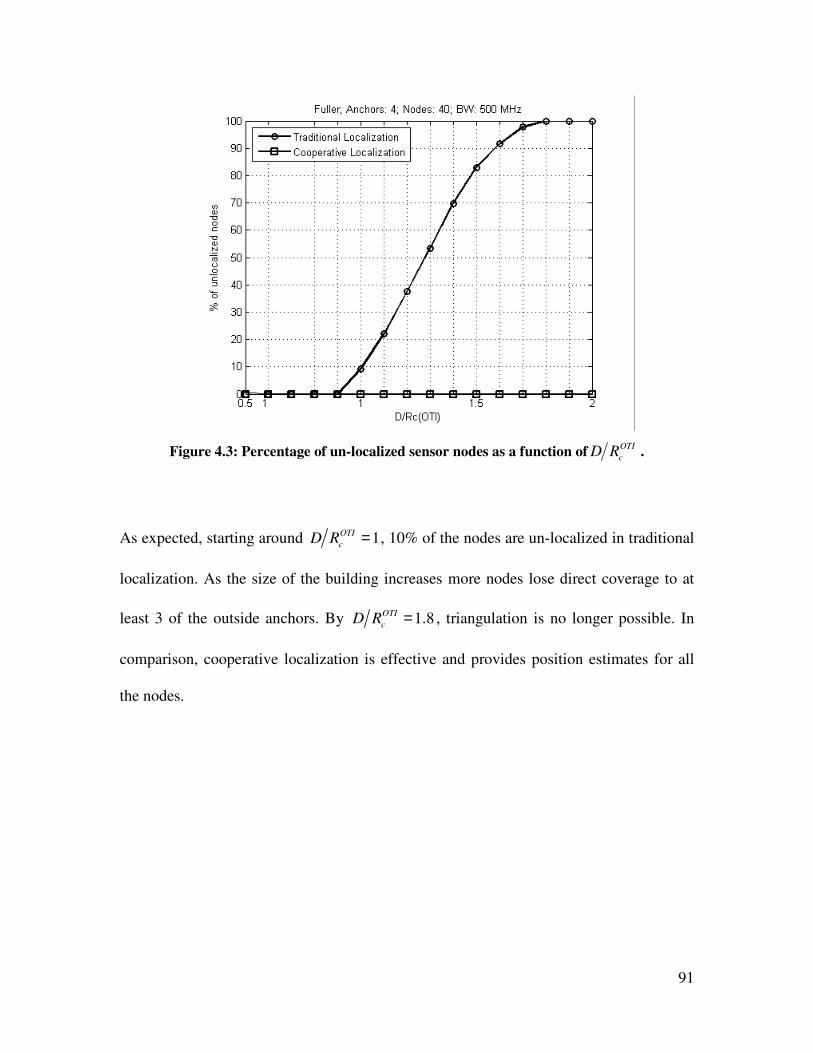
91
Figure 4.3: Percentage of un-localized sensor nodes as a function ofOTI
cD R .
As expected, starting around 1OTI
cD R = , 10% of the nodes are un-localized in traditional
localization. As the size of the building increases more nodes lose direct coverage to at
least 3 of the outside anchors. By 1.8OTI
cD R = , triangulation is no longer possible. In
comparison, cooperative localization is effective and provides position estimates for all
the nodes.
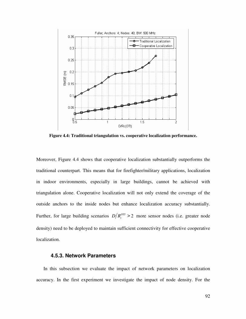
92
Figure 4.4: Traditional triangulation vs. cooperative localization performance.
Moreover, Figure 4.4 shows that cooperative localization substantially outperforms the
traditional counterpart. This means that for firefighter/military applications, localization
in indoor environments, especially in large buildings, cannot be achieved with
triangulation alone. Cooperative localization will not only extend the coverage of the
outside anchors to the inside nodes but enhance localization accuracy substantially.
Further, for large building scenarios 2OTI
cD R > more sensor nodes (i.e. greater node
density) need to be deployed to maintain sufficient connectivity for effective cooperative
localization.
4.5.3. Network Parameters
In this subsection we evaluate the impact of network parameters on localization
accuracy. In the first experiment we investigate the impact of node density. For the
93
simulation we fixed the number of anchors to be 4 and the dimension of the building to
be 25D = m and increased the number of nodes, i.e. node density which is defined by
2S N D= . 5000 Monte Carlo simulations were carried out (50 different topologies and
100 simulations per topology). The latter is needed, since the ranging conditions and
WSN connectivity are governed by Bernoulli random variables G and X . Figure 4.5
shows the simulated results for 500 MHz modeling parameters.
Figure 4.5: Localization performance as a function of node density in different indoor
environments using 500 MHz models.
Office buildings, AK and Fuller, exhibit the worst performance especially in sparse
densities. Norton, a manufacturing floor, shows the best localization accuracy among the
different buildings. This is expected since the manufacturing building’s interior is an
open-space with cluttered machines and metallic beams which is reflected in the ranging
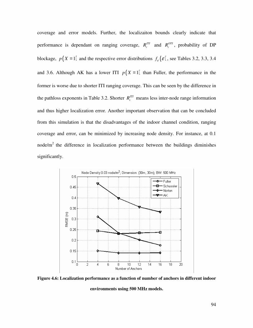
94
coverage and error models. Further, the localizaiton bounds clearly indicate that
performance is dependant on ranging coverage, ITI
cR and OTI
cR , probability of DP
blockage, ( )1p X = and the respective error distributions ( )fε ε , see Tables 3.2, 3.3, 3.4
and 3.6. Although AK has a lower ITI ( )1p X = than Fuller, the performance in the
former is worse due to shorter ITI ranging coverage. This can be seen by the difference in
the pathloss exponents in Table 3.2. Shorter ITI
cR means less inter-node range information
and thus higher localization error. Another important observation that can be concluded
from this simulation is that the disadvantages of the indoor channel condition, ranging
coverage and error, can be minimized by increasing node density. For instance, at 0.1
node/m2
the difference in localization performance between the buildings diminishes
significantly.
Figure 4.6: Localization performance as a function of number of anchors in different indoor
environments using 500 MHz models.
95
The impact of anchors on the localization accuracy is investigated in Figure. 4.6. In this
experiment, 5000 simulations were carried out with 30D = m, 0.03S = node/m2
and the
number of anchors were varied from 4 to 16 (anchors per side varies from 1 to 4). The
results show that the effect of increasing the number of anchors is higher in the office
buildings compared to the residential and manufacturing floor. This means that building
environments with harsher indoor multipath channels (lower ITI
cR and higher ( )1p G =
and ( )1p X = ) require more anchors around the building for a fixed amount of sensor
nodes to achieve similar localization performance as environments with “lighter”
multipath channels. Finally, comparing both Figs. 4.5 and 4.6 it is apparent that node
density has a higher impact on the localization accuracy compared with the number of
anchors. A similar observation was reported in [Sav05] where localization error exhibited
less sensitivity to the number of anchors.
4.5.4. Ranging Model Parameters
In this sub-section we investigate the impact of the ranging model parameters: system
dynamic range, ρ , ( )1p G = and ( )1p X = for 500 MHz and 3 GHz system bandwidths.
First we evaluate the localization bounds for different values of ρ which controls both
the ITI
cR and OTI
cR . In this experiment, the number of anchors is 4, 0.04S = node/m
2 and
the building dimension is 30D = m. We ran 5000 Monte Carlo simulations (100
topologies and 50 simulations per topology). Figure 4.7 shows the simulated localization
results as a function of dynamic range for different building environments and ranging
models.
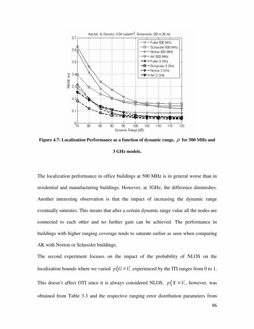
96
Figure 4.7: Localization Performance as a function of dynamic range, ρ for 500 MHz and
3 GHz models.
The localization performance in office buildings at 500 MHz is in general worse than in
residential and manufacturing buildings. However, at 3GHz, the difference diminishes.
Another interesting observation is that the impact of increasing the dynamic range
eventually saturates. This means that after a certain dynamic range value all the nodes are
connected to each other and no further gain can be achieved. The performance in
buildings with higher ranging coverage tends to saturate earlier as seen when comparing
AK with Norton or Schussler buildings.
The second experiment focuses on the impact of the probability of NLOS on the
localization bounds where we varied ( )1p G = experienced by the ITI ranges from 0 to 1.
This doesn’t affect OTI since it is always considered NLOS. ( )1p X = , however, was
obtained from Table 3.3 and the respective ranging error distribution parameters from
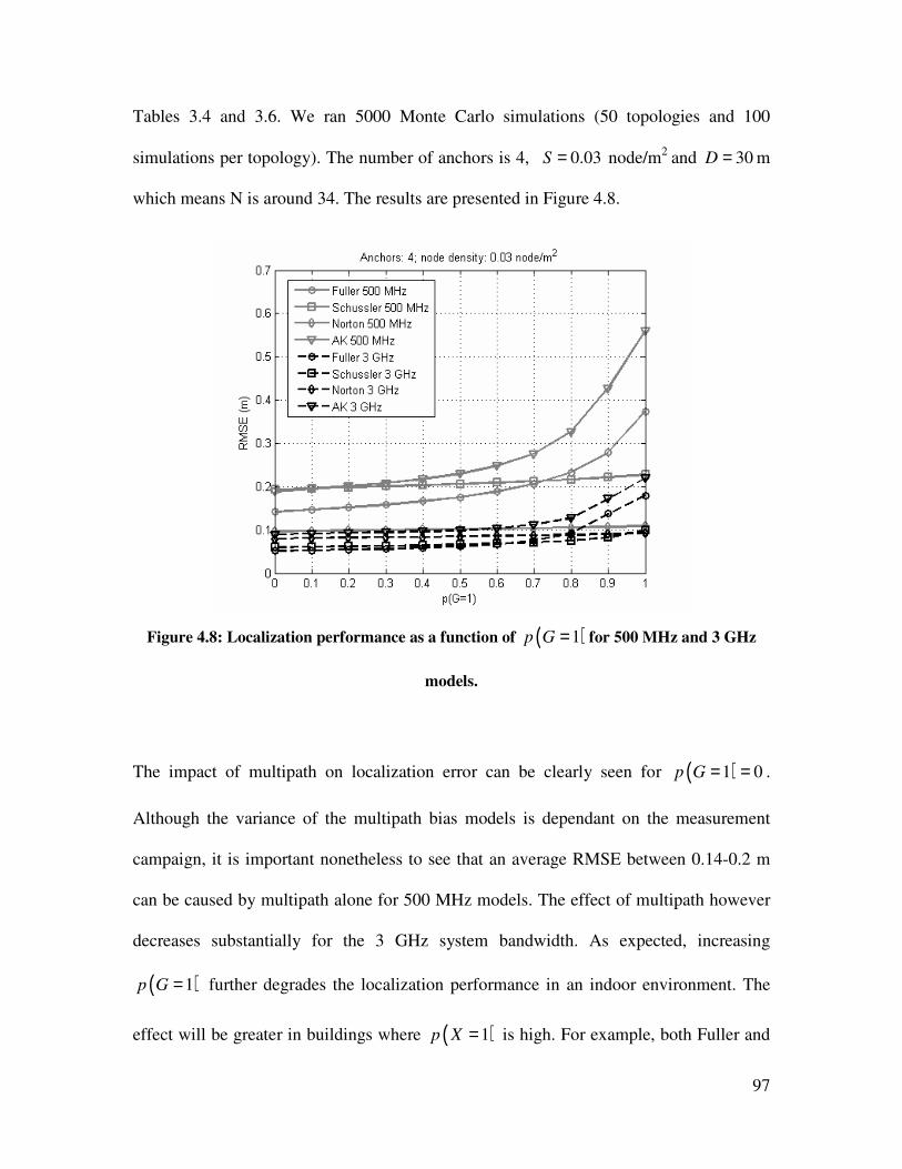
97
Tables 3.4 and 3.6. We ran 5000 Monte Carlo simulations (50 topologies and 100
simulations per topology). The number of anchors is 4, 0.03S = node/m2
and 30D = m
which means N is around 34. The results are presented in Figure 4.8.
Figure 4.8: Localization performance as a function of ( )1p G = for 500 MHz and 3 GHz
models.
The impact of multipath on localization error can be clearly seen for ( )1 0p G = = .
Although the variance of the multipath bias models is dependant on the measurement
campaign, it is important nonetheless to see that an average RMSE between 0.14-0.2 m
can be caused by multipath alone for 500 MHz models. The effect of multipath however
decreases substantially for the 3 GHz system bandwidth. As expected, increasing
( )1p G = further degrades the localization performance in an indoor environment. The
effect will be greater in buildings where ( )1p X = is high. For example, both Fuller and
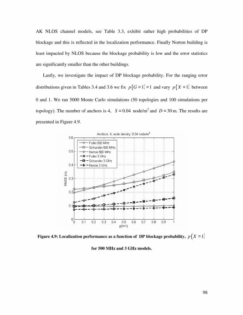
98
AK NLOS channel models, see Table 3.3, exhibit rather high probabilities of DP
blockage and this is reflected in the localization performance. Finally Norton building is
least impacted by NLOS because the blockage probability is low and the error statistics
are significantly smaller than the other buildings.
Lastly, we investigate the impact of DP blockage probability. For the ranging error
distributions given in Tables 3.4 and 3.6 we fix ( )1 1p G = = and vary ( )1p X = between
0 and 1. We ran 5000 Monte Carlo simulations (50 topologies and 100 simulations per
topology). The number of anchors is 4, 0.04S = node/m2
and 30D = m. The results are
presented in Figure 4.9.
Figure 4.9: Localization performance as a function of DP blockage probability, ( )1p X =
for 500 MHz and 3 GHz models.
99
For this specific experiment, results for AK were not available because ( )1 1p G = = ,
which means that the ITI ranges are always NLOS and thus shorter ranging coverage. In
AK’s case, the WSNs in all the simulations were ill-connected. Nonetheless, the results in
the other buildings show that increasing ( )1p X = worsens the localization error. Norton
is an exception, since the statistics of the ranging error in the presence and absence of the
DP are close to each other (see Tables 3.4 & 3.6). The impact of blockage probability on
office buildings is the highest, since the statistical distribution of the lognormal biases
exhibits a higher “variance” compared to manufacturing or residential buildings. This can
be seen in the Fuller model in Table 3.6 where such an environment exhibits a heavier
tailed distribution of the spatial ranging errors [Als07b, Als08a]. For these conditions,
when the DP blockage occurs, larger number of MPCs are lost causing higher ranging
error. Finally it is interesting to note that the impact of system bandwidth has limitations
in areas where heavier construction and obstacles separate sensor nodes. This can be seen
by comparing the impact of bandwidth on the localization performance in Schussler and
Fuller.
4.6. Conclusion
In this chapter we provided an analysis of cooperative localization bounds for WSNs
based on empirical models of UWB TOA-based OTI and ITI ranging in indoor multipath
environments. We verified the need for cooperative localization in applications where
indoor sensor nodes lack sufficient coverage to outdoor anchor nodes. We also verified
that in addition to extending coverage, cooperative localization has potential for
improving accuracy. In addition we provided a comprehensive evaluation of the
100
limitations imposed by the indoor multipath environment on cooperative localization
performance in multi-hop WSNs.
Simulation results showed that increasing node density improves localization
accuracy and can improve performance on indoor multipath channels. Increasing the
number of anchors however has greater impact on harsh indoor environments such as
office buildings due to shorter ranging coverage, i.e. less inter-node connectivity. For the
ranging model parameters, localization is constrained by the ranging coverage, statistics
of ranging error, probability of NLOS, probability of DP blockage and bandwidth. In
general, office building structures introduce higher probability of NLOS/DP blockage
and shorter ranging coverage (higher DP penetration loss and pathloss exponent) which
means higher localization error. Manufacturing floors and residential buildings on the
other hand exhibit better performance due to “lighter” indoor channel conditions. Also,
increasing the system bandwidth has the effect of improving accuracy although reduces
ranging coverage. The localization performance in office buildings exhibited less
sensitivity to changes in bandwidth because the range measurements faced harsher
obstacles such as metallic doors, vending machines and elevators.
As for the cooperative localization application for firefighter or military operations, it
is clear that in order to improve accuracy numerous nodes must be deployed in the indoor
environment alongside those attached to the personnel. In addition to providing the
necessary network density required for effective localization, these stationary nodes can
constantly provide ranging/localization information which further improves performance
in dense cluttered environments.
101
Future work in this area should aim to extend the analysis to 3-dimensions where RTI
ranging can provide coverage extension to multi-floor buildings. Further measurements
and modeling are needed to analyze the ranging error beyond ranging coverage.
Specifically the behavior of the biases and measurement time variations with distance
must be evaluated for different ranging scenarios and environments. Finally, research in
localization algorithms for indoor-specific WSNs is needed to identify and mitigate
NLOS biased range measurements in order to achieve acceptable localization
performance.
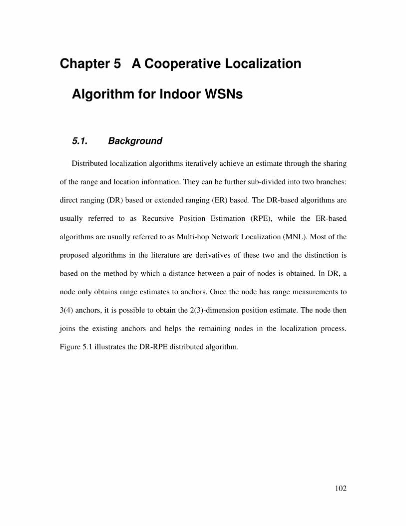
102
Chapter 5 A Cooperative Localization
Algorithm for Indoor WSNs
5.1. Background
Distributed localization algorithms iteratively achieve an estimate through the sharing
of the range and location information. They can be further sub-divided into two branches:
direct ranging (DR) based or extended ranging (ER) based. The DR-based algorithms are
usually referred to as Recursive Position Estimation (RPE), while the ER-based
algorithms are usually referred to as Multi-hop Network Localization (MNL). Most of the
proposed algorithms in the literature are derivatives of these two and the distinction is
based on the method by which a distance between a pair of nodes is obtained. In DR, a
node only obtains range estimates to anchors. Once the node has range measurements to
3(4) anchors, it is possible to obtain the 2(3)-dimension position estimate. The node then
joins the existing anchors and helps the remaining nodes in the localization process.
Figure 5.1 illustrates the DR-RPE distributed algorithm.
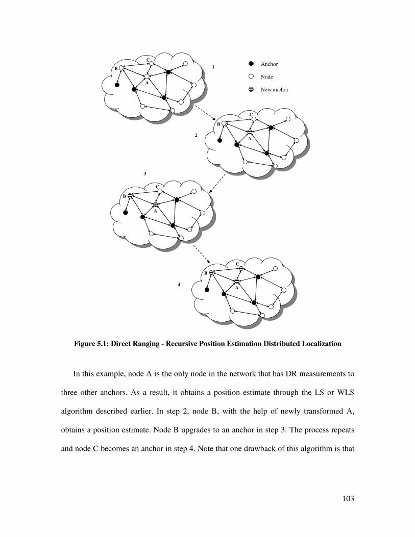
103
1
2
3
Anchor
Node
New anchor
4
A
B
C
A
B
C
A
B
C
A
B
C
Figure 5.1: Direct Ranging - Recursive Position Estimation Distributed Localization
In this example, node A is the only node in the network that has DR measurements to
three other anchors. As a result, it obtains a position estimate through the LS or WLS
algorithm described earlier. In step 2, node B, with the help of newly transformed A,
obtains a position estimate. Node B upgrades to an anchor in step 3. The process repeats
and node C becomes an anchor in step 4. Note that one drawback of this algorithm is that
104
it is possible that some nodes on the edge of the network lack sufficient direct
connectivity anchors and thus are unable to localize themselves.
In the case of ER, however, nodes attempt to estimate the distances between
themselves and a fixed pool of anchors. The nodes will obtain the distance estimate
through a variety of methods, including counting the number of hops to an anchor,
measuring the distance to the anchor (adding all distances in the path) or more accurately
trying to obtain a geometric estimate of the distance by relying on the relative location of
nodes surrounding it. In other words, nodes extend their range to anchors by measuring
and cooperating to provide an estimate of their distances to an anchor, which is beyond
their coverage. Figure 5.2 provides an example of ER distributed localization.
B
C
A
B
C
A
Anchor
Node
Extended Range
Figure 5.2: Extended Ranging - Multi-hop Distributed Localization
In this example, nodes A, B and C attempt to estimate their distances to the fixed
anchors. Once they have that information, they localize themselves. In this fashion,
nodes that are not in the direct range of the anchors get a best-effort estimate of the range.
Intuitively, DR-based algorithms are more accurate because there is no error
105
accumulation in the range information. The major draw-back of DR-based algorithms,
however, is the requirement for a certain node and anchor densities. The advantages
include very accurate localization and substantially less error propagation. DR-based
algorithms have been reported in [Alb01, Als06a, Als06b]. ER-based algorithms, on the
other hand, have less reliable error characteristics because the distance to an anchor is not
measured. Instead, it is estimated by either the number of hops or geometric estimation.
Although ER-based algorithms have less stringent requirements on the densities of
anchors and nodes, they exhibit substantial error propagation characteristics, which
explain the divergence problems that some of the algorithms in the literature have
reported. ER-based algorithms have been used in N-hop multilateration [Savr01], Robust
Positioning Algorithm [Savr01, Savr02], and Ad-hoc Positioning Algorithm (APS)
[Nic01].
The ER-MNL algorithm is easier to implement than the DR-RPE because the multi-
hop positioning algorithm requires a minimum of three reference nodes within the whole
operational field, assuming mobile nodes can communicate with all reference nodes
through multi-hop communications, while the RPE algorithm has a stricter requirement
on the deployment density of reference nodes and mobile nodes. For example, when the
deployment density of reference nodes or mobile nodes is low, in some situations, the
iterative process may not be able to continue due to the lack of nodes in the close
neighborhood.
In this chapter we introduce a novel DR-RPE distributed algorithm that incorporates a
mechanism for robust iterative node-anchor transformation. The algorithm named
Cooperative LOcalization with Quality of Estimation (CLOQ) essentially relies on its
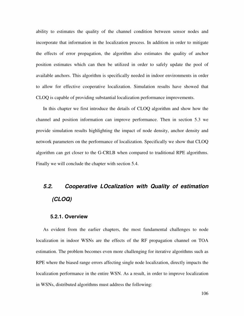
106
ability to estimates the quality of the channel condition between sensor nodes and
incorporate that information in the localization process. In addition in order to mitigate
the effects of error propagation, the algorithm also estimates the quality of anchor
position estimates which can then be utilized in order to safely update the pool of
available anchors. This algorithm is specifically needed in indoor environments in order
to allow for effective cooperative localization. Simulation results have showed that
CLOQ is capable of providing substantial localization performance improvements.
In this chapter we first introduce the details of CLOQ algorithm and show how the
channel and position information can improve performance. Then in section 5.3 we
provide simulation results highlighting the impact of node density, anchor density and
network parameters on the performance of localization. Specifically we show that CLOQ
algorithm can get closer to the G-CRLB when compared to traditional RPE algorithms.
Finally we will conclude the chapter with section 5.4.
5.2. Cooperative LOcalization with Quality of estimation
(CLOQ)
5.2.1. Overview
As evident from the earlier chapters, the most fundamental challenges to node
localization in indoor WSNs are the effects of the RF propagation channel on TOA
estimation. The problem becomes even more challenging for iterative algorithms such as
RPE where the biased range errors affecting single node localization, directly impacts the
localization performance in the entire WSN. As a result, in order to improve localization
in WSNs, distributed algorithms must address the following:
107
• The quality of TOA-based range measurements must be assessed and integrated
into the position estimation.
• The quality of the estimated node position must be assessed and integrated into
the iterative node-anchor transformation procedure.
The incorporation of these two major points is necessary in order to mitigate the effects
of the indoor channel, reduce the divergence in the solution and control error
propagation. These will ultimately provide enhanced localization accuracy which can
enable effective WSNs communication and localization in indoor environments.
In order to clarify these estimation criteria we refer to Figure 5.3 which provides an
illustrative explanation of the concept of quality.
Figure 5.3: Quality of range measurements & position estimates. (a) Bad geometry but
acceptable range measurements. (b) Good geometry but unreliable measurements.
In Figure 5.3 (a), node 1 has two LOS range measurements and one DP blocked range
measurements but its geometrical configuration results in a bad GDOP. On the other
hand, although node 2 in Figure 5.3 (b) has a better GDOP, its range measurements to the
λ
η
β
β
β
1
2 λ
(a) (b)
108
anchors are not reliable. Specifically it has three NLOS ranges with two of them the DP
is blocked. It would be therefore desirable from a performance point of view to be able to
quantify the impact of these propagation and network constraints on the localization
accuracy of nodes 1 and 2.
CLOQ is an iterative distributed algorithm that addresses these two issues by
incorporating the range measurement information and the confidence of the position
estimates. The algorithm has 4 stages:
1. Channel Identification & Mitigation: sensor nodes perform TOA ranging to
available anchor nodes and identify the channel conditions. The channel
conditions can be either λ (LOS), η (NLOS – DP) or β (NLOS – NDP). Please
refer to Figure 4.2 for further clarifications.
2. Position Estimation: Once a node receives range information from at least 3
anchors (for 2-dimensional localization) it performs localization using WLS
algorithm described earlier. The weights in WLS algorithm are created by
combining the ranging weights with the position confidence weights of the
selected anchors. The node then computes its own position and confidence index
and enters into anchor nominee phase.
3. Anchor Nomination: the potential anchor nominees then compare their position
confidence by broadcasting their information to other direct-hop nominees and the
node with highest variation from the norm withdraws from the process. The
remaining nominees move on to the next stage.
4. New Anchor Incorporation: anchor nominees transform into anchor nodes and
start transmitting anchor range packets to the remainder of the WSN.
109
5.2.2. Step I: Channel Identification
The statistical relationship between the RF channel and the TOA ranging error are
essential in the identification process. In [Guv07] the kurtosis of the channel was used to
distinguish between LOS and NLOS. In [Hei07], on the other hand, the statistics of the
propagation channel such as RMS delay spread, mean excess delay, total signal power
and their combination were used in order to identify between the presence and absence of
the DP. In this dissertation we use the first path power (FPP) and the total signal power
(TP) in order to identify between LOS, NLOS/DP and NLOS/NDP. As a result a sensor
node would examine the measured FPP and TP and attempt to identify the channel
condition. This is then used to weigh the TOA range measurements to the respective
anchors in order to further improve the localization performance.
Using the measurement database introduced in chapter 3, we can analyze the statistical
relationship between the power and the channel condition. Accordingly we divide the
database into OTI and ITI and their respective ranging conditions such as illustrated in
Figure 5.4. Instead of analyzing the FPP or TP individually we decide to examine their
ratio. Therefore we define the following ratio
1
1
pL
kk
αδ
α=
=∑
(5.1)
where pL is the number of MPCs, and kα is the amplitude of the kth
path. In (5.1), 1α
refers to the first path power. In the case the first path power is the DP then 1DPα α= .

110
Figure 5.4: Database classification for channel identification
We are then interested in examining the conditional PDFs given by ( )|fδ δ λ , ( )|fδ δ η
and ( )|fδ δ β in ITI; and ( )|fδ δ η and ( )|fδ δ β in OTI. This distinction is both
physically sound and necessary since the characteristics of the signal propagating on an
ITI range are different from those propagating on an OTI. Specifically for the latter, all
the MPCs must penetrate the exterior of the building in order to reach the indoor sensor
node. In practical implementation sensor nodes can identify ITI from OTI ranges by
examining the node ID in the transmitted packet. We assume here that OTI anchors will
have unique IDs that can be easily identified from the interior sensor nodes.
First we provide the statistical analysis of the ITI measurements. Figure 5.5 provides the
results for ITI data at 500 MHz and 3 GHz.
ITI OTI
λ (LOS)
η (NLOS – DP)
β (NLOS – NDP)
η (NLOS – DP)
β (NLOS – NDP)
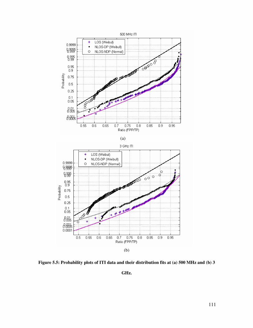
111
Figure 5.5: Probability plots of ITI data and their distribution fits at (a) 500 MHz and (b) 3
GHz.
(a)
(b)
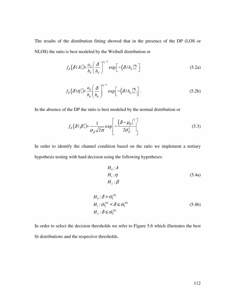
112
The results of the distribution fitting showed that in the presence of the DP (LOS or
NLOS) the ratio is best modeled by the Weibull distribution or
( ) ( )1
| exp /
a
aaf b
b b
λ
λλδ λ
λ λ
δδ λ δ−
= − (5.2a)
( ) ( )1
| exp /
a
aaf b
b b
η
ηηδ η
η η
δδ η δ−
= − . (5.2b)
In the absence of the DP the ratio is best modeled by the normal distribution or
( ) ( )2
2
1| exp
22f
βδ
ββ
δ µδ β
σσ π
− = −
(5.3)
In order to identify the channel condition based on the ratio we implement a tertiary
hypothesis testing with hard decision using the following hypotheses:
0
1
2
:
:
:
H
H
H
ληβ
(5.4a)
0 1
1 2 1
2 2
:
:
:
ITI
ITI ITI
ITI
H th
H th th
H th
δδ
δ
>
< ≤
≤
(5.4b)
In order to select the decision thresholds we refer to Figure 5.6 which illustrates the best
fit distributions and the respective thresholds.
113
Figure 5.6: Distribution fits and the respective thresholds. (a) 500 MHz and (b) 3 GHz.
2
ITIth
1
ITIth
2
ITIth
1
ITIth
(a)
(b)
114
A similar analysis and decision framework can be followed for OTI ranges. The
probability plots are provided in Figure 5.7. The data are best modeled by the Weibull
distribution in the presence of the DP and normal in the absence and they can also be
represented by (5.2b) and (5.3).
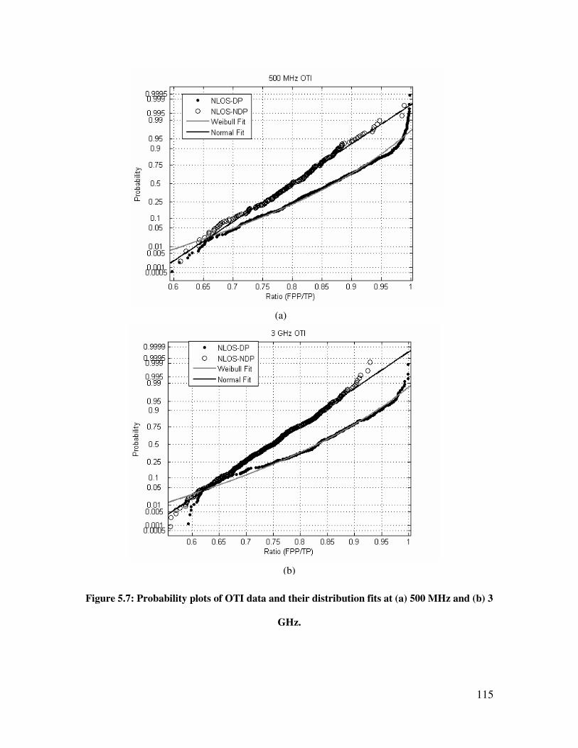
115
Figure 5.7: Probability plots of OTI data and their distribution fits at (a) 500 MHz and (b) 3
GHz.
(a)
(b)
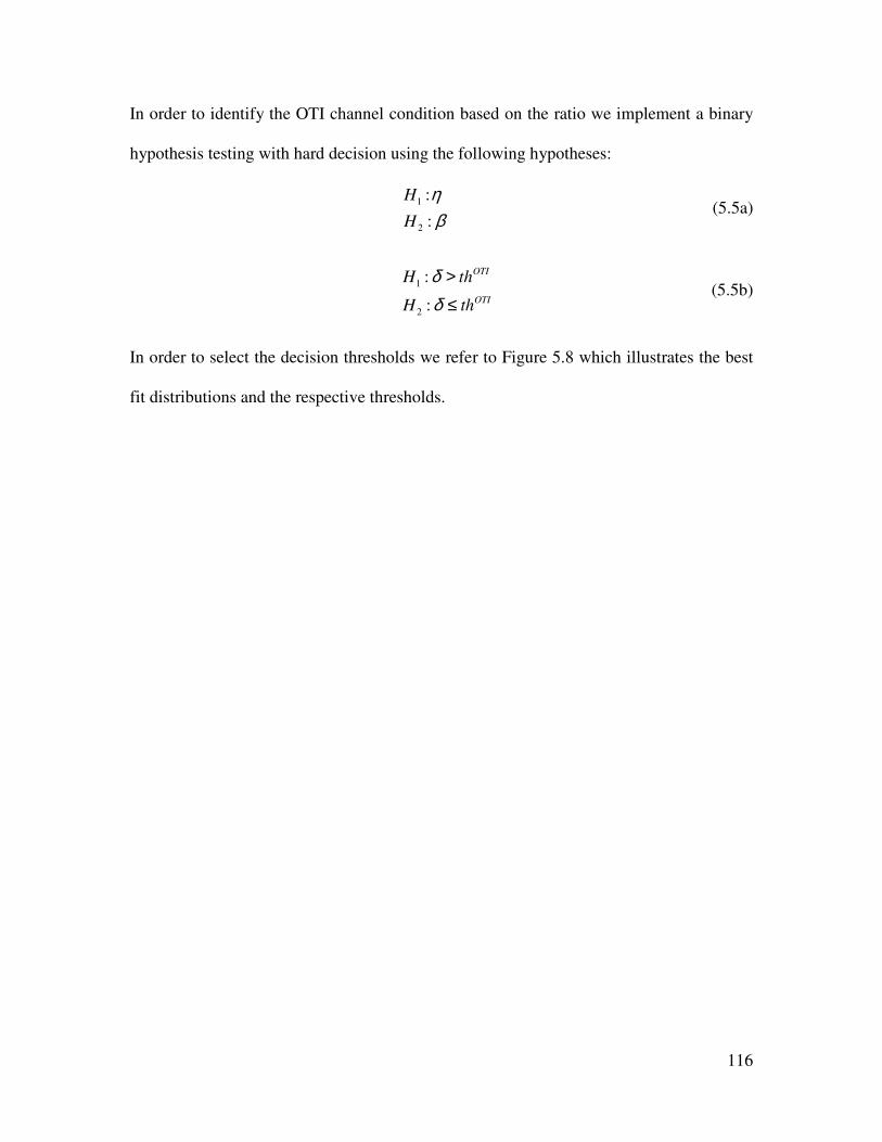
116
In order to identify the OTI channel condition based on the ratio we implement a binary
hypothesis testing with hard decision using the following hypotheses:
1
2
:
:
H
H
ηβ
(5.5a)
1
2
:
:
OTI
OTI
H th
H th
δδ
>
≤ (5.5b)
In order to select the decision thresholds we refer to Figure 5.8 which illustrates the best
fit distributions and the respective thresholds.
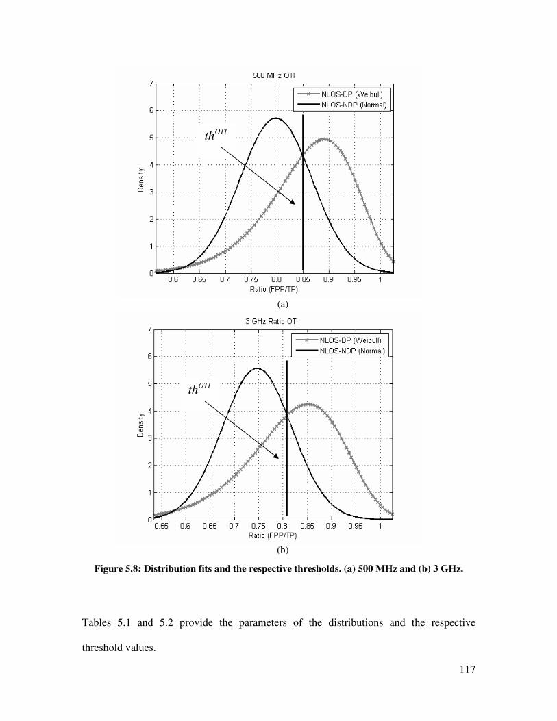
117
Figure 5.8: Distribution fits and the respective thresholds. (a) 500 MHz and (b) 3 GHz.
Tables 5.1 and 5.2 provide the parameters of the distributions and the respective
threshold values.
OTIth
(a)
(b)
OTIth
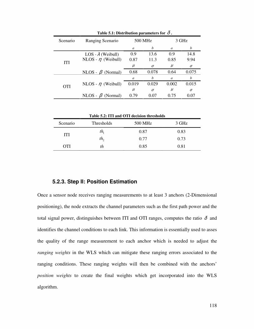
118
Table 5.1: Distribution parameters for δ .
Scenario Ranging Scenario 500 MHz 3 GHz
a b a b
LOS - λ (Weibull) 0.9 13.6 0.9 14.8
NLOS - η (Weibull) 0.87 11.3 0.85 9.94
µ σ µ σ ITI
NLOS - β (Normal) 0.68 0.078 0.64 0.075
a b a b
NLOS - η (Weibull) 0.019 0.029 0.002 0.015
µ σ µ σ OTI
NLOS - β (Normal) 0.79 0.07 0.75 0.07
Table 5.2: ITI and OTI decision thresholds
Scenario Thresholds 500 MHz 3 GHz
1th 0.87 0.83 ITI
2th 0.77 0.73
OTI th 0.85 0.81
5.2.3. Step II: Position Estimation
Once a sensor node receives ranging measurements to at least 3 anchors (2-Dimensional
positioning), the node extracts the channel parameters such as the first path power and the
total signal power, distinguishes between ITI and OTI ranges, computes the ratio δ and
identifies the channel conditions to each link. This information is essentially used to asses
the quality of the range measurement to each anchor which is needed to adjust the
ranging weights in the WLS which can mitigate these ranging errors associated to the
ranging conditions. These ranging weights will then be combined with the anchors’
position weights to create the final weights which get incorporated into the WLS
algorithm.
119
In general, at a given instant in the distributed localization process, a sensor node with
the coordinates ( ),T
n n nx y=θθθθ can be connected to M exterior anchors with coordinates
( ),TOTI
m m mx y=θθθθ and U interior newly transformed anchors with coordinates
( ),TITI
u u ux y=θθθθ , where [ ]0,n N∈ and [ ],0m M∈ − and [ ]0,u U∈ , respectively. The
node will receive range measurements from the respective anchors and form a range
measurement vector given by ( )1 1ˆ ˆ ˆ ˆˆ , , , , ,
T
n nM n nUd d d d=d ⋯ ⋯ . Associated with this vector
the node extracts the first path and total signal power from the ranging signals and forms
the ratio vector ( )1 1, , , , ,T
n nM n nUδ δ δ δ=δ ⋯ ⋯ according to (5.1). By comparing the ratio
vector to the thresholds in Table 5.1 the sensor node identifies the condition of the
channel be it λ (LOS), η (NLOS – DP) or β (NLOS – NDP). Once the channel is
identified, the node uses the available ranging error models presented in chapter 3 to
generate the de-normalized weights. In both λ (LOS) and η (NLOS – DP), the ranging
error is normally distributed and as a result the weights can be obtained by the inverse of
the de-normalized variance or,
( )/ 2
1
ˆw
dλ η
σ= , (5.6)
where σ is the standard deviation of the normalized ranging error and d is the biased
range measurement. In the case the ranging condition is β (NLOS – NDP), the ranging
error is lognormally distributed and the weight can then be obtained by the following,
( ) 2
2
1ˆexp 2 log 2 1w dβ µ σσ
= − + + × + (5.7)

120
where µ and σ are the mean and standard deviation of the normalized ranging error’s
logarithm and the values are presented in chapter 3.
The position weights on the other hand are obtained by the inverse of the position
variance of the anchors. Original anchors (which are located outside) are assumed to have
no position errors and thus zero variance. Newly transformed anchors on the other hand
compute their position variance from the error covariance given by [Shi01],
( ) 11T
−−=C H W H (5.8)
and the position variance is then ( )2
p traceσ = C . In actual implementation (5.8) needs to
be re-orientated and thus singular value decomposition (SVD) is usually performed
before extracting 2
xσ and 2
yσ of the position error covariance.
The weighting matrix W that is used in the WLS algorithm and (5.8) is given by
( )1 1, , , , ,M Udiag w w w w=W ⋯ ⋯ , where i
w is a combination of the range measurement
weight g
w and the position weight p
w or formally given by
( ) ( )1
1/ 1/i
g p
ww w
=+
. (5.9)
This weighting method implies that the higher the error position variance the smaller the
weight (less contribution in the overall weight and thus WLS localization). Similarly, the
higher the ranging error variance the lower is the ranging weight g
w and thus the lower
the weight in (5.9). This ensures that range or position incorporated into the WLS is
weighed according to their respective quality.

121
In order to clarify the weighting procedure it is best to resort to a simple example. Figure
5.9 provides a localization example where node 6 is trying to obtain its localization
information at the ith
iteration of the algorithm.
Figure 5.9: CLOQ Algorithm – Stage II position estimation. Black circles are anchors, grey
circles are newly transformed anchors and white circles are un-localized sensor nodes.
In Figure 5.9, external anchors have identification numbers that are distinct from indoor
nodes. Specifically, ( )1 1 8 8, , , ,TOTI
x y x y− − − −=θ … while the interior nodes have positive
IDs. In addition note that due to initial setup we assume that the exterior anchors have a
knowledge of their coordinates without any position errors, that is 2 ( ) 0p mσ = where
6
6
2
ˆ
ˆ(6) : ?
p
x
y
σ
=
2( 1) : 0pσ− =
2( 8) : 0pσ− =
2( 7) : 0pσ− =
2( 6) : 0pσ− =
2( 2) : 0pσ− =
2( 3) : 0pσ− =
2( 4) : 0pσ− =
2( 5) : 0pσ− =
2(10) : 0.1pσ =
2(2) : 0.6pσ =
1β−
2λ
8λ− 10η
122
[ ]8, 1m ∈ − − . At any given instant during the localization process nodes can be connected
to a combination of original and newly formed anchors. In the example provided in
Figure 5.9, node 6 is connected to original anchors with IDs: -8 and -1; and to newly
transformed anchors with IDs: 10 and 2. CLOQ algorithm provides a mechanism to
estimate the location information by incorporating the statistical uncertainties of the
range measurements and the anchors’ position errors. According to the signal powers the
node receives from the anchors (not shown here), an identification of the channel
conditions leads to two LOS, one NLOS DP and one NLOS NDP. Node 6 then forms a
table of this information in order to create the weights necessary for the WLS algorithm.
Table 5.3 provides an overview of the connectivity information node 6 observes.
Table 5.3: Connectivity information that node 6 gathers about surrounding anchors.
Range Channel Range Weight Anchor Position Weight Final Weight
Position Weight 6, 1d −
NLOS-NDP wβ 21/p pw σ= = ∞ ( )6, 1
1
1/w
wβ− =
6, 8d − LOS wλ 21/p pw σ= = ∞ ( )6, 8
1
1/w
wλ− =
6,10d NLOS-DP wη 21/ 10p pw σ= = ( ) ( )6,10
1
1/ 1/ p
ww wη
=+
6,2d LOS wλ 21/ 1.67p pw σ= = ( ) ( )6,2
1
1/ 1/ p
ww wλ
=+
The range weights in Table 5.3 can be obtained from (5.6) and (5.7). Also note that in
this example, node 6 is connected to two original anchors (-1 and -8) and this is reflected
in the final weights. Node 6 uses the weights ( )6, 1 6, 8 6,10 6,2, , ,diag w w w w− −=W in the
WLS to estimate its own position. For more details about the WLS algorithm please refer
to chapter 2. Finally node 6 uses (5.9) to compute the covariance of the position error and
123
thus the position variance 2 (6)pσ . The estimated position ( )6 6ˆ ˆ,x y and the position
variance 2 (6)pσ are then broadcast to entire WSN in order to aid the remaining sensor
node in the localization process.
5.2.4. Step III: Anchor Nomination
Once a node has estimated its position coordinate and its position variance it enters
into anchor nominee stage where it broadcasts and listens to nominee packets. The main
purpose for this stage is to ensure that nominees with a very bad position estimate do not
transform into anchors and thus reduce error propagation. In addition only anchor
nominees broadcast, receive and forward nominee packets. Thus the other sensor nodes
do not forward nominee packets. This ensures the prevention of excessive flooding of
messages which can cause performance degradation. For further clarification we refer to
Figure 5.10 where we assume the network is at a jth iteration where several anchor
nominees are comparing their position variance.
124
Figure 5.10: CLOQ Algorithm – Stage III Anchor Nomination. Black circles are anchor
nodes, grey circles are anchor nominees and white circles are un-localized sensor nodes.
In this example, after broadcasting and forwarding, nominees 1, 2, 3 and 4 will be able to
compare their quality of position estimate. Only anchor nominee 4 withdraws from the
anchor transformation process, since its position variance is substantially higher than the
rest. It thus has to wait for future iterations in order to transform. In addition, note that
anchor nominee 5 is not connected to any other nominees. In this case it assumes it’s the
only one in the network and proceeds in the transformation. This approach ensures that
isolated parts of the WSN will be able to localize effectively.
2(1) : 0.4pσ =
2(2) : 0.1pσ =
2(3) : 0.01pσ = 2(4) : 5.3pσ =
2(5) : 1.2pσ =
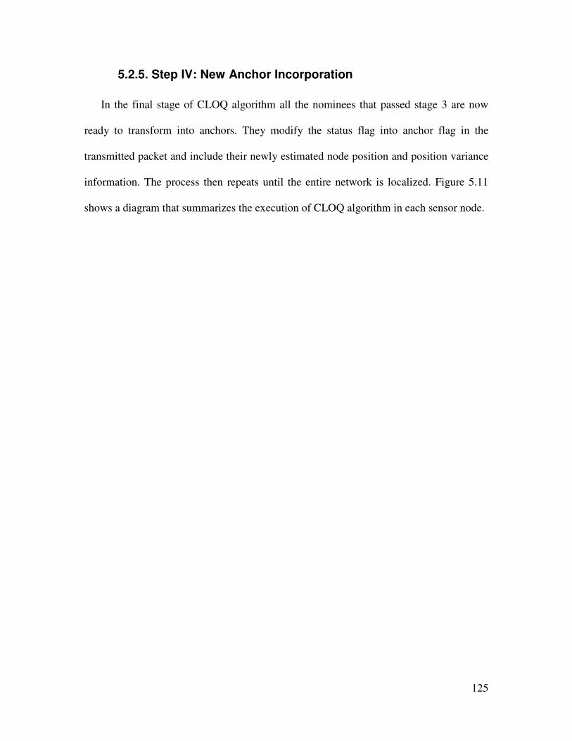
125
5.2.5. Step IV: New Anchor Incorporation
In the final stage of CLOQ algorithm all the nominees that passed stage 3 are now
ready to transform into anchors. They modify the status flag into anchor flag in the
transmitted packet and include their newly estimated node position and position variance
information. The process then repeats until the entire network is localized. Figure 5.11
shows a diagram that summarizes the execution of CLOQ algorithm in each sensor node.
126
Figure 5.11: CLOQ Algorithm flow diagram
Range Measurements/Packets
to at least 3
Range Quality
( )1, , Kδ δ…
Extract Info
Position Variance
( )2 2
1, ,p pK
σ σ…
K ranges to anchors
Generate Ranging
Weights
Generate Anchor
Weights WLS
Algorithm
( )2ˆ ˆ, ,ii i p
x y σ
Anchor Position
( )1 1, , , ,K Kx y x y…
Yes
Anchor Nominee:
Compare 2
ipσ with
other nominees
Large Deviation
from Mean
Anchor
Transformation
Broadcast Anchor
Packets
No
Node Mode
No Yes
127
5.3. Performance Analysis
5.3.1. Simulation Setup
The simulation setup is based on the application of firefighters or soldiers requiring
localization in indoor environments. M anchors are distributed evenly around the building
where they are placed 1 m away from the exterior wall, see Fig. 4.1. N sensor nodes are
then uniformly distributed inside the building. Connectivity is assumed between node-
node and anchor-node if the respective TOA range measurements are within ITI and OTI
ranging coverage, ITI
cR and OTI
cR , respectively. The simulations were carried out using
the models from chapter 3. The dynamic range of the system, ρ , is set to 90 dB and this
parameter controls the ranging coverage and the number of inter-node range
measurements in the WSN. For example at 500 MHz bandwidth and 90 dB dynamic
range, ITI
cR will correspond roughly to 15-30 m depending on the LOS or NLOS
condition and building environment. Similarly, OTI
cR will be around 5-10 m depending on
the building type. We set the measurement noise z
σ equal to 20 mm. For most
simulations, unless otherwise stated, the probability of NLOS, ( )1p G = , was set to 0.5.
The probability of blockage, ( ) ( )21p X p ζ= = , however, was obtained from the
measurement results in Table 3.3. The ranging conditions and the WSN inter-node
connectivity are ultimately governed by the random variables G and X , see (4.1). The
first path power and total signal power were simulated from the empirical pathloss
models.
128
For the analysis of the simulations we compute the average RMS of the location error of
each WSN topology. The RMSE is computed by
( ) ( )( ) 2 21
2 2 1i i
N
x yN N
i
tr
RMSEN N
σ σ−
× × × =
+ = =
∑J
, (5.10)
where ( )tr ⋅ is the trace operation. 2
ixσ and 2
iyσ are the diagonal elements of the ith
diagonal sub-matrix of ( ) ( )
1
2 2N N
−
× × × J . The average RMSE is obtained by averaging
(5.10) over the total number of topologies and simulations.
5.3.2. Node Density
In the first experiment we investigate the impact of node density. For the simulation
we fixed the number of anchors to 8 and the dimension of the building to 20D = m and
increased the number of nodes, i.e. node density which is defined by 2S N D= . 5000
Monte Carlo simulations were carried out (100 different topologies and 50 simulations
per topology). The latter is needed, since the ranging conditions and WSN connectivity
are governed by Bernoulli random variables G and X .
Figure 5.12 shows the results for fuller building using 3 GHz models. We have
chosen one of the worst indoor building environments in order to test the ability of
CLOQ in improving performance. The comparative performance of the buildings is
provided in chapter 4. In addition to the CLOQ algorithm, we have simulated a typical
LS distributed algorithm that doesn’t have any channel or position quality incorporation.
It is clear from the figure that the CLOQ algorithm mitigates ranging errors in indoor
environments, improves the performance and approaches the lower bound.
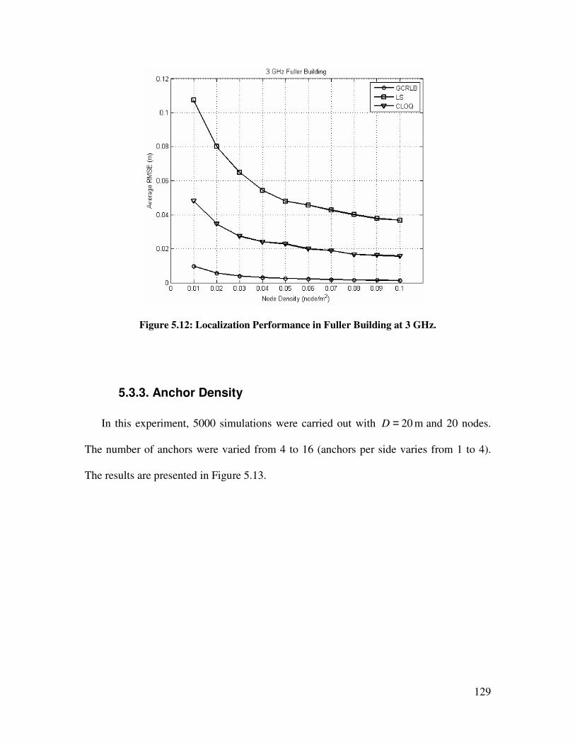
129
Figure 5.12: Localization Performance in Fuller Building at 3 GHz.
5.3.3. Anchor Density
In this experiment, 5000 simulations were carried out with 20D = m and 20 nodes.
The number of anchors were varied from 4 to 16 (anchors per side varies from 1 to 4).
The results are presented in Figure 5.13.
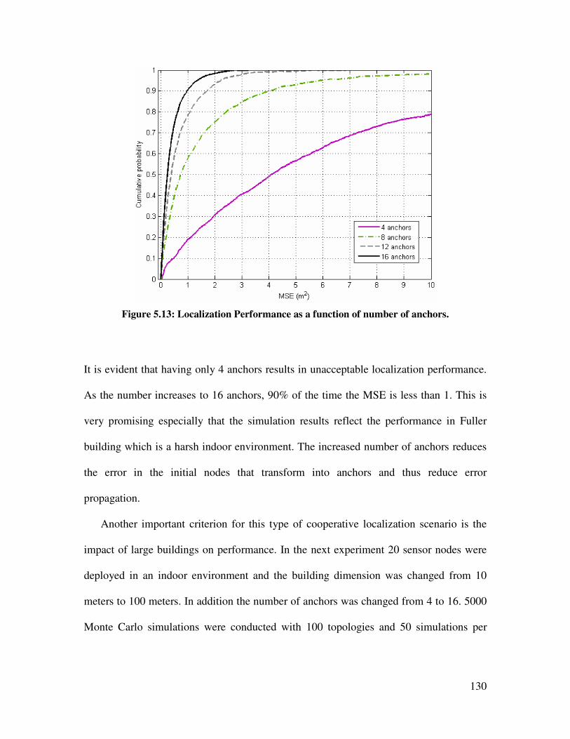
130
Figure 5.13: Localization Performance as a function of number of anchors.
It is evident that having only 4 anchors results in unacceptable localization performance.
As the number increases to 16 anchors, 90% of the time the MSE is less than 1. This is
very promising especially that the simulation results reflect the performance in Fuller
building which is a harsh indoor environment. The increased number of anchors reduces
the error in the initial nodes that transform into anchors and thus reduce error
propagation.
Another important criterion for this type of cooperative localization scenario is the
impact of large buildings on performance. In the next experiment 20 sensor nodes were
deployed in an indoor environment and the building dimension was changed from 10
meters to 100 meters. In addition the number of anchors was changed from 4 to 16. 5000
Monte Carlo simulations were conducted with 100 topologies and 50 simulations per
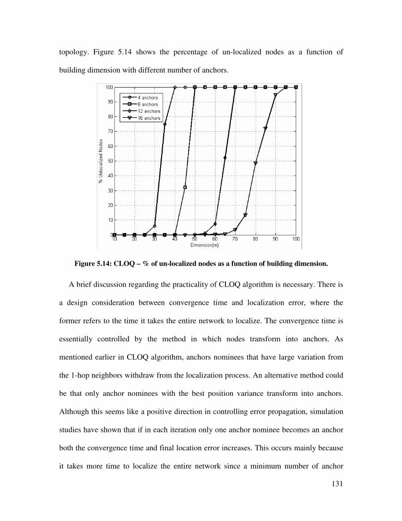
131
topology. Figure 5.14 shows the percentage of un-localized nodes as a function of
building dimension with different number of anchors.
Figure 5.14: CLOQ – % of un-localized nodes as a function of building dimension.
A brief discussion regarding the practicality of CLOQ algorithm is necessary. There is
a design consideration between convergence time and localization error, where the
former refers to the time it takes the entire network to localize. The convergence time is
essentially controlled by the method in which nodes transform into anchors. As
mentioned earlier in CLOQ algorithm, anchors nominees that have large variation from
the 1-hop neighbors withdraw from the localization process. An alternative method could
be that only anchor nominees with the best position variance transform into anchors.
Although this seems like a positive direction in controlling error propagation, simulation
studies have shown that if in each iteration only one anchor nominee becomes an anchor
both the convergence time and final location error increases. This occurs mainly because
it takes more time to localize the entire network since a minimum number of anchor
132
nodes are transformed in each iteration. The increase in localization error is due to the
enhanced impact of geometry induced errors on the localization process. Less anchors at
each stage means a higher chance of nodes having “bad” geometry according to the
GDOP mentioned earlier. This means that in each iteration it is important to maximize
the number of node-anchor transformation. Even newly transformed anchors with high
position variance can help to reduce geometry errors and overall position errors through
the WLS approach.
133
Chapter 6 Conclusion & Future Work
6.1. Conclusion
In this dissertation we have described a comprehensive UWB measurement and
modeling campaign that was aimed to characterize the spatial behavior of indoor TOA-
based ranging. In addition we provided an analysis of cooperative localization bounds for
WSNs based on empirical models of UWB TOA-based OTI and ITI ranging in indoor
multipath environments. Finally we integrated the channel information and developed a
novel cooperative localization algorithm CLOQ that is specifically suitable for the indoor
WSNs.
The measurement and modeling involved spatial characterization. This involved
analyzing and modeling the coverage and accuracy of ranging in indoor environments.
The measurement involved four different building environments: residential, old office,
modern office and manufacturing floor and three different ranging scenarios ITI, OTI and
RTI. We showed that ranging coverage is inversely related to the bandwidth of the
system and the harshness of the ranging scenario and environment. In addition, ranging
error can be modeled as normal and lognormal in the presence and the absence of the DP,
respectively. Furthermore, the modeling parameters are affected by the ranging scenario,
environment and system bandwidth. The modeling results in this dissertation provide an
experimental analysis of the physical constraints imposed by the dense cluttered indoor
environments on TOA-based UWB ranging. In addition the models should help
134
researchers obtain localization bounds specific to indoor environments which are
important to assess and evaluate the limitations facing different localization algorithms.
As for cooperative localization we verified the need for such technology in applications
where indoor sensor nodes lack sufficient coverage to outdoor anchor nodes. We also
verified that in addition to extending coverage, cooperative localization has potential for
improving accuracy. In addition we provided a comprehensive evaluation of the
limitations imposed by the indoor multipath environment on cooperative localization
performance in multi-hop WSNs.
Simulation results showed that increasing node density improves localization
accuracy and can improve performance in indoor multipath channels. Increasing the
number of anchors however has greater impact in harsh indoor environments such as
office buildings due to shorter ranging coverage, i.e. less inter-node connectivity. For the
ranging model parameters, localization is constrained by the ranging coverage, statistics
of ranging error, probability of NLOS, probability of DP blockage and bandwidth. In
general, office building structures introduce higher probability of NLOS/DP blockage
and shorter ranging coverage (higher DP penetration loss and pathloss exponent) which
means higher localization error. Manufacturing floors and residential buildings on the
other hand exhibit better performance due to “lighter” indoor channel conditions. Also,
increasing the system bandwidth, although reduces ranging coverage, has the effect of
improving accuracy. The localization performance in office buildings exhibited less
sensitivity to changes in bandwidth because the range measurements faced harsher
obstacles such as metallic doors, vending machines and elevators. As for the cooperative
localization application for firefighter or military operations, it is clear that in order to
135
improve accuracy numerous nodes must be deployed in the indoor environment alongside
those attached to the personnel. In addition to providing the necessary network density
required for effective localization, these stationary nodes can constantly provide
ranging/localization information which further improves performance in dense cluttered
environments.
Finally simulation results of the CLOQ algorithm showed that incorporating the
quality of the range and position estimation can substantially improve the localization
performance in WSNs.
6.2. Future Work
As we have seen throughout the dissertation, TOA-based ranging and localization
face many challenges in indoor environments. Potential applications that require high
localization accuracy need novel techniques in localization. One of the most promising
alternatives is cooperative localization in WSNs using UWB signals. The UWB signals
have shown to be able to combat multipath error in indoor environments, while
cooperative localization mitigates the channel impairments and further extends the
coverage of the anchor nodes.
Future work in this area should continue the measurements and modeling in order to
analyze the ranging error beyond ranging coverage. Specifically the behavior of the
biases and measurement time variations with distance must be evaluated for different
ranging scenarios and environments. In addition the analysis of cooperative localization
must extend the analysis to 3-dimensions where RTI ranging can provide coverage
extension to multi-floor buildings.
136
Also research in localization algorithms for indoor-specific WSNs is needed to
identify and mitigate NLOS biased range measurements in order to achieve acceptable
localization performance. It would be therefore pertinent for nodes to be able to range
and localize with precise information regarding the channel conditions.
Another important research direction is analyzing and characterizing error
propagation in WSN localization. One of the major problems to accurate localization in
iterative distributed algorithms is error propagation. Algorithms must therefore be able to
incorporate methodologies which can help in controlling or even reducing error
propagation so that nodes on the edge of networks do estimate reliable position
information.
137
References
[Aky02] I. Akyildz, W. Su, Y. Sankarasubramaniam and E. Cayirci, “A survey on
sensor networks”, IEEE Communications Magazine, vol. 40, no. 8, pp.
102-114, Aug. 2002.
[Ala03a] B. Alavi, K. Pahlavan, “Bandwidth effect on distance error modeling for
indoor geolocation”, IEEE Proceeding on Personal, Indoor and Mobile
Communications, vol. 3, pp. 2198-2202, Sept. 2003.
[Ala03b] B. Alavi, K. Pahlavan, “Modeling of the distance error for indoor
geolocation”, IEEE Wireless Communications and Networking
Conference (WCNC), vol. 1, pp. 668-672, March 2003.
[Ala05] B. Alavi and K. Pahlavan, “Analysis of undetected direct path in time of
arrival based UWB indoor geolocation”, in Proceedings of the IEEE
Vehicular Technology Conference, vol. 4, pp. 2627-2631, Dallas, TX,
USA, September, 2005.
[Ala06] B. Alavi, K. Pahlavan, “Modeling of the TOA-based distance
measurement error using UWB indoor radio measurements”, IEEE
Communications Letters, vol. 10, no. 4, pp. 275-277, April 2006.
[Alb01] J. Albowicz, A. Chen and L. Zhang, “Recursive position estimation in
sensor networks”, in Proc. of 2001 IEEE International Conference on
Network Protocols (ICNP’01), Riverside, CA, pp. 35-41, Nov. 2001.
138
[Alj04] S. Al-Jazzar, “Algorithms and parameter estimation for radiolocation in
NLOS environments”, Ph.D. dissertation, University of Cincinnati,
Cincinnati, OH, 2004.
[Als06a] N. Alsindi, K. Pahlavan, B. Alavi and X. Li, “A novel cooperative
localization algorithm for indoor sensor networks”, in Proc. of 2006 IEEE
International Symposium on Personal Indoor and Mobile Radio
Communications (PIMRC ’06), Helsinki, Finland, pp. 1-6, Sept. 2006.
[Als06b] N. Alsindi, K. Pahlavan, B. Alavi, “An error propagation aware algorithm
for precise cooperative indoor localization”, in Proc. of IEEE Military
Communications Conference (MILCOM), Washington D.C., pp. 1-7,
October, 2006.
[Als07a] N. Alsindi, B. Alavi, K. Pahlavan, “Empirical pathloss model for indoor
geolocation using UWB measurements”, IEE Electronic Letters, vol. 43,
no. 7, pp. 370-372, March 2007.
[Als07b] N. Alsindi, B. Alavi, K. Pahlavan, “Spatial characteristics of UWB TOA-
based ranging in indoor multipath environments” in Proc. of IEEE
International Symposium on Personal Indoor and Mobile Radio
Communications (PIMRC) ’07, Athens, Greece, pp. 1-6, Sept. 2007.
[Als08a] N. Alsindi, B. Alavi, K. Pahlavan, “Measurement and modeling of UWB
TOA-based ranging in indoor multipath environments”, accepted
manuscript to be published in IEEE Transactions on Vehicular
Technology, 2008.
[Als08b] N. Alsindi, K. Pahlavan, “Cooperative localization bounds for indoor ultra
139
wideband sensor networks”, EURASIP ASP special issue on Cooperative
Localization in Wireless Ad Hoc and Sensor Networks, vol. 2008, article
ID 852509, pp. 1-13, April 2008.
[Als08c] N. Alsindi, M. Heidari and K. Pahlavan, “Blockage identification in
indoor UWB TOA-based ranging using Multi Band OFDM signals”, in
Proc. IEEE Wireless Communications and Networking Conference, Las
Vegas, NV, April 2008.
[Als08d] N. Alsindi and K. Pahlavan, “Node Localization”, Wireless Sensor
Networks: A Networking Perspective, Wiley – IEEE Press, to appear,
2008.
[Bah00a] P. Bahl and V. Padmanabhan, “RADAR: an in-building RF-based user
location and tracking system,” in Proceedings of 19th
Annual Joint
Conference of the IEEE Computer and Communications Societies
(INFOCOM), vol. 2, Tel Aviv, Israel, March 2000, pp. 775-784.
[Bah00b] P. Bahl, V. Padmanabhan and A. Balachandran, “Enhancements to the
RADAR User Location and Tracking System,” Tech. Rep. MSR-TR-00-
12, Microsoft Research, Feb. 2000.
[Ber04] J. Berlant, Y. Goegebeur, J. Segers, J. Teugels, Statistics of Extremes:
Theory and Applications, Wiley, 2004.
[Bet04] A. Betra, et. Al, Multi-band OFDM Physical Layer Proposal for IEEE
802.15 Task Group 3a, Sept. 2004.
[Bot04] C. Botteron, A. Host-Madsen and M. Fattouche, “Effects of system and
environment parameters on the performance of network-based mobile
140
station position estimators”, IEEE Transactions on Vechicular
Technology, vol. 53, no. 1, pp. 163-180, Jan. 2004.
[Cha06] C. Chang and A. Sahai, “Cramer-Rao-type bounds for localization”,
EURASIP Journal on Applied Signal Processing, vol. 2006, article ID
94287, pp. 1-13, 2006.
[Caf98] J. Caffery and G. Stuber, “Subsriber location in CDMA cellular
networks”, IEEE Transactions on Vehicular Technology, vol. 47, no. 2,
pp. 406-416, May 1998.
[Cas88] E. Castillo, Extreme Value Theory in Engineering, New York: Academic,
1988.
[Che99] P. –C Chen, “A non-line-of-sight error mitigation algorithm in location
estimation,” IEEE Wireless Communications and Networking Conference
(WCNC’ 99), New Orleans, LA, USA, Sept. 1999, pp. 316-320.
[Cho05] C.-C. Chong, S.K. Yong, “A generic statistical-based UWB channel
model for high-rise apartments”, IEEE Transactions on Antennas and
Propagation, vol. 53, no. 8, pp. 2389-2399, Aug. 2005.
[Chu03] W.C. Chung and D. Ha, “An accurate ultra wideband ranging for precision
asset location”, IEEE Conference on Ultra Wideband Systems and
Technologies (UWBST), pp. 389-393, Nov. 2003.
[Den04] B. Denis, and N. Daniele, “NLOS ranging error mitigation in a distributed
positioning algorithm for indoor UWB ad-hoc networks”, in Proc. of IEEE
International Workshop on Wireless Ad-hoc Networks (IWWAN), pp. 356-
360, Oulu, Finland, May-Jun. 2004.
141
[Dum94] L. Dumont, M. Fattouche and G. Morrison, “Super-resolution of multipath
channels in a spread spectrum location system”, IEE Electronic Letters,
vol. 30, no. 19, pp. 1583-1584, Sept. 1994.
[Dur98] G. Durgin, T.S. Rappaport and H. Xu, “Measurements and models for
radio pathloss and penetration loss in and around homes and trees at 5.85
GHz”, IEEE Transactions on Communications, vol. 46, no. 11, pp. 1484-
1496, Nov. 1998.
[Fal06] C. Falsi, D. Dardari, L. Mucchi and M.Z. Win, “Time of arrival estimation
for UWB Localizers in realistic environments”, EURASIPJournal on
Applied Signal Processing, vol. 2006, article ID 32082, pp. 1-13, 2006.
[Fon02] R. J. Fontana and S. J Gunderson, “Ultra-wideband precision asset
location system”, in Proc. of IEEE Conference on UWB Systems and
Technolgies (UWBST), Baltimore, MD, May 2002, pp.147-150.
[Gha04] S.S. Ghassemzadeh, R. Jana, C.W. Rice, W. Turin and V. Tarokh,
“Measurement and modeling of an ultra-wide bandwidth indoor channel”,
IEEE Transactions on Communications, vol. 52, no. 10, pp. 1786-1796,
Oct. 2004.
[Ghav04] M. Ghavami, L.B. Michael and R. Kohno, Ultra-wideband Signals and
Systems in Communication Engineering, Wiley, Hoboken, NJ, 2004.
[Guv07] I. Guvenc, C.-C. Chong and F. Watanabe, “NLOS identification and
mitigation for UWB localization systems” IEEE Wireless
Communications and Networking Conference (WCNC) ’07, pp. 1571-
1576, Hong Kong, China, March 11-15 2007.
142
[Gez05] S. Gezici, Z. Tian, G.B. Giannakis, H. Kobayashi, A.F. Molisch, H.V.
Poor and Z. Sahinoglu, “Localization via ultra-wideband radios: a look at
positioning aspects for future sensor networks,” IEEE Signal Processing
Magazine, vol. 22, no. 4, pp. 70-84, July 2005.
[Hat06] A. Hatami, K. Pahlavan, M. Heidari and F. Akgul, “On RSS and TOA
based indoor geolocation – a comparative performance evaluation”, in
Proceedings of the IEEE Wireless Communications and Networking
Conference (WCNC), vol.4, pp. 2267-2272, Las Vegas, NV, USA, April
2006.
[Hei07] M. Heidari, F.O. Akgul and K. Pahlavan, “Identification of the absence of
direct path in indoor localization systems” in Proc. IEEE International
Symposium on Personal Indoor and Mobile Radio Communications
(PIMRC) ’07, Athens, Greece, pp. 1-6, Sept. 2007.
[How90] S. J. Howard and K. Pahlavan, “Measurement and Analysis of the indoor
Radio Channel in the Frequency Domain”, IEEE Transactions on
Instrumentation and Measurements, no. 39, pp. 751-55, Oct. 1990.
[Jai01] R. Jain, A. Puri, and R. Sengupta, “Geographical routing using partial
information for wireless ad hoc networks,” IEEE Personal
Communications Magazine, vol. 8, no. 1, Feb. 2001, pp. 48-57.
[Jou06b] D.B. Jourdan, D. Dardari and M.Z. Win, “Position error bound and
localization accuracy outage in dense cluttered environments”, in
Proceedings of IEEE International Conference on Ultra-Wideband, pp.
519-524, Boston, MA, USA, Sept. 2006.
143
[Jou06a] D.B. Jourdan, D. Dardari and M.Z. Win, “Position error bound for UWB
localization in dense cluttered environments”, in Proceedings of IEEE
Int’l Conf. on Commun. (ICC) ’06, vol. 8, pp. 3705-3710, Istanbul,
Turkey, June, 2006.
[Kap96] E.D. Kaplan, Understanding GPS: Principles and Applications, Artech
House, Norwood, MA, 1996.
[Kay93] S.M. Kay, Fundementals of Statistical Signal Processing: Estimation
Theory, Prentice Hall, Upper Saddle River, New Jersey, 1993.
[Ko98] Y. Ko and N.H. Vaidya, “Location-aided routing (LAR) in mobile adhoc
networks,” in Proceedings of the Association for Computing Machinery
(ACM)/IEEE Mobile Computing and Networking (MOBICOM), Dallas,
TX, Oct. 1998, pp. 66-75.
[Koo98] H. Koorapaty, H. Grubeck and M. Cedervall, “Effect of biased
measurement errors on accuracy of position location methods”, in IEEE
Global Communications Conference (GLOBECOMM) ’98, vol. 3, pp.
1497-1502, 1998.
[Kos00] H. Koshima and J. Hoshen, “Personal locator services emerge”, IEEE
Spectrum, vol. 37, no. 2, Feb. 2000. pp. 41-48.
[Kri99] P. Krishnamurthy and K. Pahlavan, “Radio propagation modeling for
indoor geolocation applications,” in Proceedings of IEEE Personal,
Indoor and Mobile Radio Communications, PIMRC’99, Kyoto, Japan, pp.
446-450, Sept. 1999.
[Lar04] E.G. Larsson, “Cramer-Rao bound analysis of distributed positioning in
144
sensor networks”, IEEE Signal Processing Letters, vol. 11, no. 3, pp. 334-
337, March 2004.
[Li04] X. Li and K. Pahlavan, “Super-resolution TOA estimation with diversity
for indoor geolocation”, IEEE Transactions on Wireless Communications,
vol. 3, no. 1, pp. 224-234, Jan. 2004.
[Lee02] J.-Y. Lee and R.A. Scholtz, “Ranging in a dense multipath environment
using an UWB radio link”, IEEE Transactions on Selected Areas in
Communications, vol. 20, no. 9, pp.1677-1683, Dec. 2002.
[Lee06] J.-Y. Lee and S. Yoo, “Large error performance of UWB ranging in
multipath and multiuser environments”, IEEE Transactions on Microwave
Theory and Techniques, vol. 54, no. 4, pp. 1887-1895, April 2006.
[Low05] Z.N. Low, J.H. Cheong, C.L. Law, W.T. Ng and Y.J. Lee, “Pulse
detection algorithm for line-of-sight (LOS) UWB ranging applications”,
IEEE Antennas and Wireless Propagation Letters, vol. 4, pp. 63-67, 2005.
[Mar05] S. Markose, A. Alentorn, “Option pricing and the implied tail index with
the generalized extreme value distribution”, Computing in Economics and
Finance, 396, Society for Computation Economics, 2005.
[McG02] J. McGeough, “Wireless location positioning based on signal propagation
data”, White Paper, http://www.wirelessdevnet.com/software/, 2002.
[Mis02] P. Misra and P. Enge, Global Positioning System: Signals, Measurements
and Performance, Ganga-Jamuna Press, Lincoln, MA, 2002.
[Mol05] A.F. Molisch, “Ultrawideband propagation channel-theory, measurement
and modeling”, IEEE Transactions on Vehicular Technology, vol. 54, no.
145
5, pp. 1528-1545, Sept. 2005.
[Muq06] A. Muqaibel, A. Safaai-Jazi, A. Attiya, B. Woerner and S. Riad, “Path-
loss and time dispersion parameters for indoor UWB propagation”, IEEE
Transactions on Wireless Communications, vol. 5, no. 3, pp. 550-559,
March 2006.
[Nic01] D. Niculescu and B. Nath, “Ad-hoc positioning system”, in Proc. of 2001
IEEE Global Communications Conference (Globecomm ’01), San
Antonio, TX, pp. 2926-2931, Nov. 2001.
[Opp04] I. Oppermann, M. Hamalainen and J. Iinatti, UWB Theory and
Applications, Wiley, Hoboken, NJ, 2004.
[Pah98] K. Pahlavan, P. Krishnamurthy and J. Beneat, “Wideband radio
propagation modeling for indoor geolocation applications,” IEEE
Communications Magazine, vol. 36, no. 4, pp. 60-65, April 1998.
[Pah00] K. Pahlavan, P. Krishnamurthy, A. Hatami, M. Ylianttila, J. Makela, R.
Pichna and J. Vallstrom, “Handoff in hybrid mobile data networks (invited
paper),” IEEE Personal Communications Magazine, vol. 7, no. 2, Apr.
2000, pp. 34-47.
[Pah02] K. Pahlavan, X. Li, and J. Makela, "Indoor geolocation science and
technology," IEEE Communications Magazine, vol. 40, no. 2, pp. 112-
118, Feb. 2002.
[Pah05] K. Pahlavan, A. H. Levesque, Wireless Information Networks, 2nd
edition,
John Wiley, 2005.
146
[Pah06] K. Pahlavan, F.O. Akgul, M. Heidari, A. Hatami, J.M. Elwell and R.D.
Tingley, “Indoor geolocation in the absence of the direct path”, IEEE
Wireless Communications Magazine, vol. 13, no. 6, pp. 50-58, Dec. 2006.
[Pat03] N. Patwari, A.O. Hero, M. Perkins, N.S. Correal and R.J. O’Dea,
“Relative location estimation in wireless sensor networks”, IEEE
Transactions on Signal Processing, vol. 51, no. 8, pp. 2137-2148, August,
2003.
[Pat05] N. Patwari, J.N. Ash, S. Kyperountas, A. O. Hero, R. L. Moses and N. S.
Correal, “Locating the nodes: cooperative localization in wireless sensor
networks”, IEEE Signal Processing Magazine, vol. 22, no. 4, pp. 54-69,
July 2005.
[Por03] D. Porcino and W. Hirt, “Ultra-wideband radio technology: potential and
challenges ahead”, IEEE Communications Magazine, vol. 41, no. 7, pp.
66-74, July 2003.
[Pot00] G.J. Pottie and W.J. Kaiser, “Wireless integrated network sensors,”
Communications of the Association for Computing and Machinery (ACM),
vol. 43, no. 5, May 2000, pp. 51-58.
[Qi06] Y. Qi, H. Kobayashi, H. Suda, “Analysis of wireless geolocation in a non-
line-of-sight environment”, IEEE Transactions on Wireless
Communications, vol. 5, no. 3, pp. 672-681, March 2006.
[Roo02a] T. Roos, P. Myllymaki, H. Tirri, P. Miskangas and J. Sievanen, “A
probabilistic approach to WLAN user location estimation,” International
147
Journal of Wireless Information Networks, vol. 9, no. 3, Jul. 2002, pp.
155-164.
[Roo02b] T. Roos, P. Myllymaki and H. Tirri, “A statistical modeling approach to
location estimation,” IEEE Transactions on Mobile Computing, vol. 1, no.
1, pp. 59-69, Jan. 2002.
[Sav05] A. Savvides, W.L. Garber, R.L. Moses and M.B. Srivastava, “An analysis
of error inducing parameters in multihop sensor node localization”, IEEE
Transactions on Mobile Computing, vol. 4, no. 6, pp. 567-577, Dec. 2005.
[Savr01] C. Savarese, J.M. Rabaey and J. Beutel, “Locationing in distributed ad-hoc
wireless sensor networks”, in Proc. of 2001 International Conference on
Acoustics, Speech and Signal Processing (ICASSP’01), Salt Lake City,
UT, May 2001, pp. 2037-2040.
[Savr02] C. Savarese, K. Langendoen, and J. Rabaey, “Robust positioning
algorithms for distributed ad-hoc wireless sensor networks”, in Proce. Of
USENIX Technical Annual Conference, Monterrey, CA, Jun. 2002, pp.
317-328.
[Shi01] D. Shin, T. Sung, “Analysis of positioning errors in radionavigation
systems”, in Proceedings of IEEE Intelligent Transmission Systems
Conference, pp. 156-159, Oakland, CA, USA, August 2001.
[Siw03] K. Siwiak, H. Bertoni, and S.M. Yano, “Relation between multipath and
wave propagation attenuation”, IEE Electronic Letters, vol. 39, no. 1, pp.
142-143, Jan. 2003.

148
[Sma00] A. Smailagic and D. Koan, “Location sensing and privacy in a context-
aware computing environment,” IEEE Transactions on Wireless
Communications, vol. 9, no. 5, Oct. 2000, pp. 10-17.
[Spi01] M. Spirito, “On the accuracy of cellular mobile station location
estimation,” IEEE Transactions on Vehicular Technology, vol. 50, no. 3,
May 2001, pp. 674-684.
[Tar06] Z. Tarique, W.Q. Malik and D.J. Edwards, “Bandwidth requirements for
accurate detection of direct path in multipath environment”, IEE
Electronic Letters, vol. 42, no. 2, pp. 100-102, Jan. 2006.
[Van68] H.L. Van Trees, Detection, Estimation and Modulation Theory, Part I.
John Wiley & Sons, Inc., 1968.
[Ven07a] S. Venkatesh and R.M. Buehrer, “NLOS mitigation using linear
programming in ultra wideband location-aware networks”, IEEE
Transactions on Vehicular Technology, vol. 56, no. 5, pp. 3182-3198,
Sept. 2007.
[Ven07b] S. Venkatesh and R.M. Buehrer, “NLOS identificaiton in ultra-wideband
systems based on received signal statistics”, IET Microwave, Antennas
and Propagation, vol. 1, no. 6, pp. 1120-1130, Dec. 2007.
[Wei05] W. Wei, X. J.- Yu, Z. Z.- Liang, “A new NLOS error mitigation algorithm
in location estimation”, IEEE Transactions on Vehicular Technology, vol.
54, no. 6, pp. 2048-2053, Nov. 2005.
[Wer98] J. Werb and C. Lanzl, “Designing a positining system for finding things
and people indoors,” IEEE Spectrum, vol. 35, no. 9, Sept. 1998, pp. 71-78.

149


