Download - IDAR , F 2012 Lecture 09. Lidar Simulation and Error ...superlidar.colorado.edu/.../LidarLecture09_LidarSimulation.pdf · Lecture 09. Lidar Simulation ... lidar simulation code complete

LIDAR REMOTE SENSING PROF. XINZHAO CHU CU-BOULDER, FALL 2012

Lecture 09. Lidar Simulation and Error Analysis Overview (1)

  Introduction �

  Lidar Modeling via Lidar Simulation & Error Analysis�

  Functions of Lidar Simulation and Error Analysis�

  How to Build up Lidar Simulation?�

  Range-resolved lidar simulation �

  Signal-to-Noise Ratio (SNR) vs. error�

  Summary�

1


Introduction   Lidar simulation of return signals is a direct application of lidar

equations involving physical processes to predict the signal level and signal distribution along the lidar beam.�

  Error analysis is to understand the measurement errors and their dependence on various lidar system parameters, physical interactions, atmospheric/medium parameters, and lidar detection procedure.�

  Practice of lidar simulation and error analysis helps deepen our understanding of every process, especially physical processes, in the entire lidar detection procedure. �

  It also helps us understand how each factor in the lidar detection procedure contributes to the signal strength and the measurement errors (accuracy, precision, and resolution).�

  Introducing lidar simulation and error analysis earlier in the lidar class is to encourage students to consciously ask questions how each component in the lidar sensing procedure affects the measurements.�

  We will come back to the lidar simulation and error analysis with deeper levels after discussing actual lidar systems in details.� 2


Lidar Modeling   Why are lidar simulation and error analysis necessary?�-  Analogy to atmospheric modeling which is a complex code to integrate everything together to see what happens in a complicated system like the atmosphere. The basis is the atmospheric science theory. �-  Lidar remote sensing is a complicated procedure with many factors involved (both human-controllable and non-controllable). It is difficult to imagine what happens just from lidar theory (lidar equation). So we want to write a computer code to integrate all factors together in a proper way based on the lidar theory. By doing so we can investigate what the lidar outcome is supposed to be and how the outcome changes with the factors. �  What are the lidar simulation and error analysis?�-  The lidar simulation and error analysis are lidar modeling to integrate complicated lidar remote sensing processes together.�-  The basis for lidar simulation and error analysis is the lidar theory, spectroscopy, and measurement principles. �

3


Lidar Simulation and Error Analysis   Four Major Goals of Lidar Simulation and Error Analysis�

1.  Estimate of expected lidar returns (the lidar signal level and distribution along the lidar beam -- resolved range)�

2.  Analysis of expected measurement precision & resolution, i.e., errors (uncertainty) introduced by photon noise and trade-off among lidar parameters (e.g., off-zenith angle determination)�

3.  Analysis of expected measurement accuracy & precision (caused by uncertainty in system parameters) and lidar measurement sensitivity to atomic, lidar, and atmospheric parameters �

4.  Forward model to test data retrieval code and metrics�

4


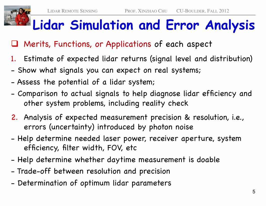
Lidar Simulation and Error Analysis   Merits, Functions, or Applications of each aspect �1.  Estimate of expected lidar returns (signal level and distribution)�- Show what signals you can expect on real systems; �- Assess the potential of a lidar system; �- Comparison to actual signals to help diagnose lidar efficiency and

other system problems, including reality check �

2.  Analysis of expected measurement precision & resolution, i.e., errors (uncertainty) introduced by photon noise�

- Help determine needed laser power, receiver aperture, system efficiency, filter width, FOV, etc�

- Help determine whether daytime measurement is doable�- Trade-off between resolution and precision �- Determination of optimum lidar parameters�

5


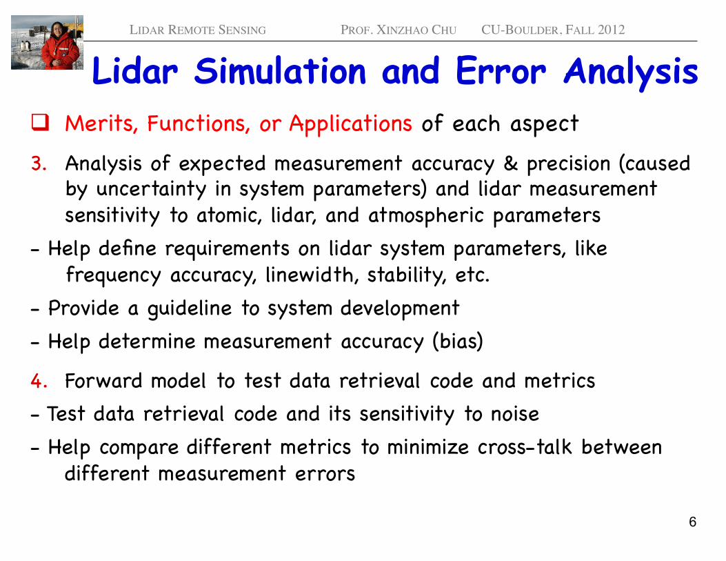
Lidar Simulation and Error Analysis   Merits, Functions, or Applications of each aspect �3.  Analysis of expected measurement accuracy & precision (caused

by uncertainty in system parameters) and lidar measurement sensitivity to atomic, lidar, and atmospheric parameters�

- Help define requirements on lidar system parameters, like frequency accuracy, linewidth, stability, etc.�

- Provide a guideline to system development �- Help determine measurement accuracy (bias)�

4.  Forward model to test data retrieval code and metrics�- Test data retrieval code and its sensitivity to noise�- Help compare different metrics to minimize cross-talk between

different measurement errors�

6


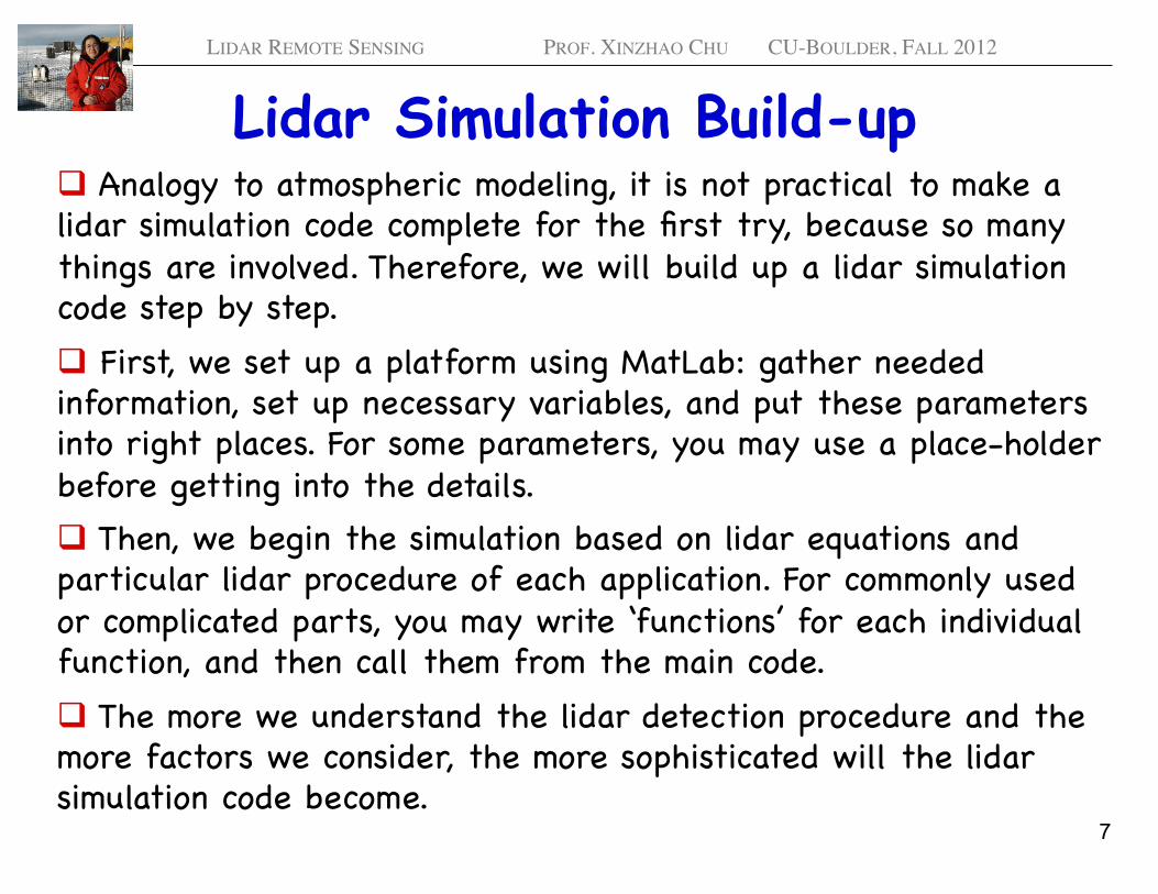
Lidar Simulation Build-up   Analogy to atmospheric modeling, it is not practical to make a lidar simulation code complete for the first try, because so many things are involved. Therefore, we will build up a lidar simulation code step by step.�  First, we set up a platform using MatLab: gather needed information, set up necessary variables, and put these parameters into right places. For some parameters, you may use a place-holder before getting into the details.�  Then, we begin the simulation based on lidar equations and particular lidar procedure of each application. For commonly used or complicated parts, you may write ‘functions’ for each individual function, and then call them from the main code.�  The more we understand the lidar detection procedure and the more factors we consider, the more sophisticated will the lidar simulation code become.�

7


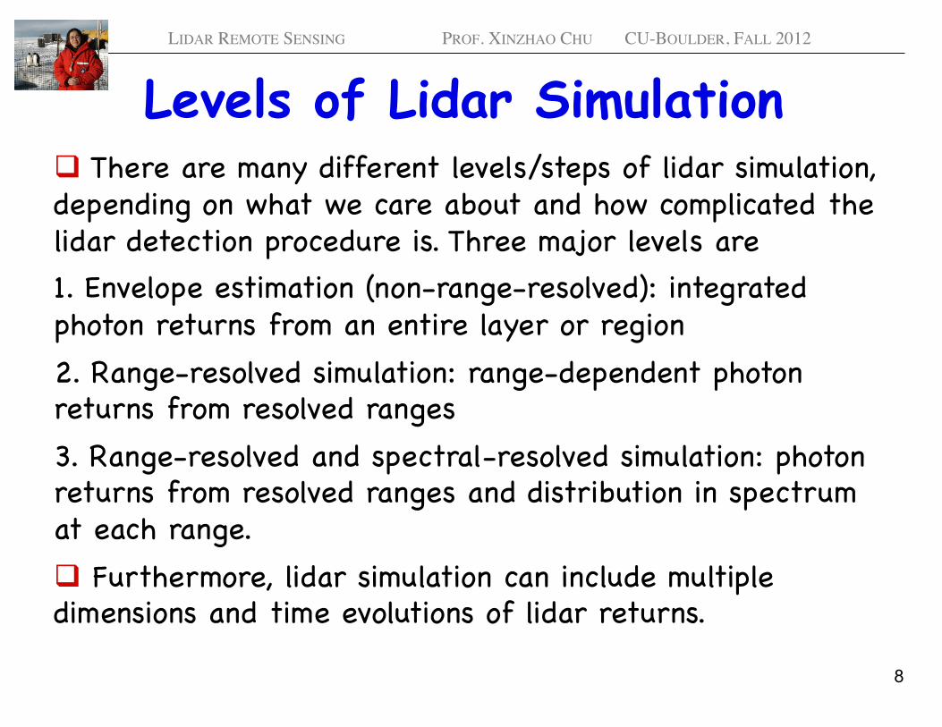
Levels of Lidar Simulation   There are many different levels/steps of lidar simulation, depending on what we care about and how complicated the lidar detection procedure is. Three major levels are�1. Envelope estimation (non-range-resolved): integrated photon returns from an entire layer or region �2. Range-resolved simulation: range-dependent photon returns from resolved ranges�3. Range-resolved and spectral-resolved simulation: photon returns from resolved ranges and distribution in spectrum at each range.�  Furthermore, lidar simulation can include multiple dimensions and time evolutions of lidar returns.�

8


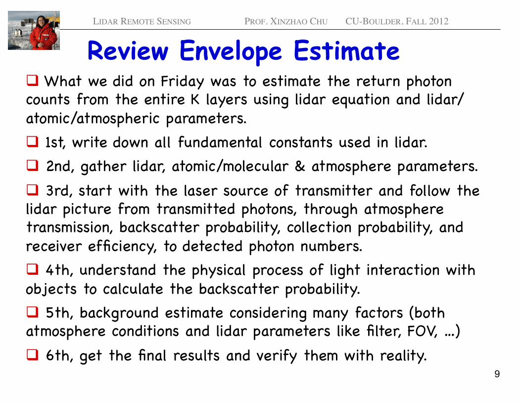
Review Envelope Estimate   What we did on Friday was to estimate the return photon counts from the entire K layers using lidar equation and lidar/atomic/atmospheric parameters.�  1st, write down all fundamental constants used in lidar.�  2nd, gather lidar, atomic/molecular & atmosphere parameters.�  3rd, start with the laser source of transmitter and follow the lidar picture from transmitted photons, through atmosphere transmission, backscatter probability, collection probability, and receiver efficiency, to detected photon numbers.�  4th, understand the physical process of light interaction with objects to calculate the backscatter probability.�  5th, background estimate considering many factors (both atmosphere conditions and lidar parameters like filter, FOV, …)�  6th, get the final results and verify them with reality.�

9


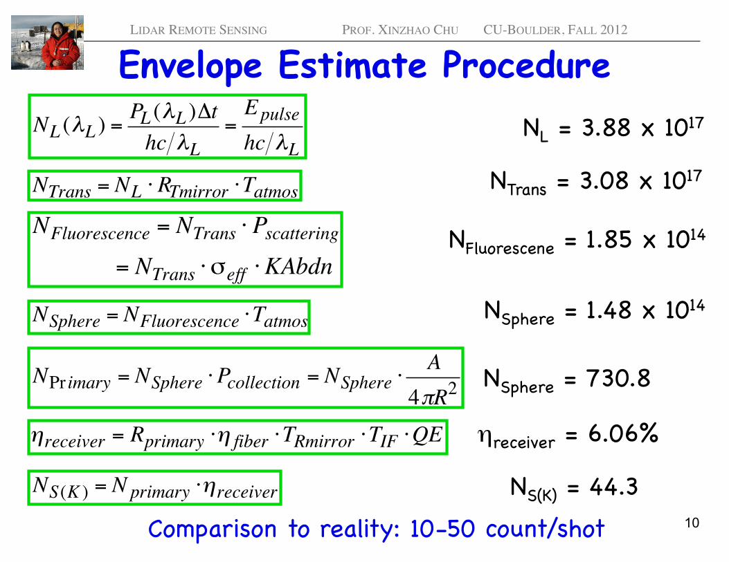
Envelope Estimate Procedure

€

NL (λL ) =PL (λL )Δthc λL

=Epulsehc λL

NL = 3.88 x 1017 �

€

NTrans = NL ⋅ RTmirror ⋅Tatmos NTrans = 3.08 x 1017 �

€

NFluorescence = NTrans ⋅ Pscattering= NTrans ⋅ σeff ⋅KAbdn

NFluorescene = 1.85 x 1014 �

€

NSphere = NFluorescence ⋅Tatmos NSphere = 1.48 x 1014 �

€

NPr imary = NSphere ⋅Pcollection = NSphere ⋅A

4πR2NSphere = 730.8 �

€

ηreceiver = Rprimary ⋅η fiber ⋅TRmirror ⋅TIF ⋅QE ηreceiver = 6.06% �

€

NS(K ) = Nprimary ⋅ηreceiver NS(K) = 44.3 �Comparison to reality: 10-50 count/shot � 10


Fundamental Constants, Lidar Parameters,

Atomic or Molecular Parameters, Atmospheric Parameters

  Always use NIST latest fundamental constants�  Try to use NIST atomic and molecular parameters�  Gather all possible lidar parameters�  Gather possible atmospheric parameters�  Another possible way is to scale from existing lidar

measurements�

11


Fundamental Constants in Lidar   Fundamental constants for lidar simulation �1)  Light speed in vacuum c�2)  Planck constant h�3)  Boltzmann constant kB �4)  Elementary charge e�5)  Electron mass me�6)  Proton mass mp �7)  Electric constant ε0 �8)  Magnetic constant µ0 �9)  Avogadro constant NA �10) ……�

12


Lidar Parameters   Lidar parameters for lidar simulation �1)  Laser pulse energy, repetition rate, pulse duration, �2)  Laser central wavelength, linewidth, chirp �3)  Laser divergence angle�4)  Transmitter mirror reflectivity�5)  Telescope primary mirror diameter and reflectivity�6)  Telescope/receiver field-of-view (FOV)�7)  Receiver mirrors’ transmission, �8)  Fiber coupling efficiency, transmission �9)  Filter peak transmission, bandwidth, out-of-band rejection �10) Detector quantum efficiency and maximum count rate�11)  ……� 13


Atomic or Molecular Parameters   Atomic and molecular parameters for lidar simulation �1)  Atomic energy level structure, degeneracy�2)  Spontaneous transition rate Aki, oscillator strength f�3)  Atomic mass or molecular weight �4)  Resonance frequency or wavelength�5)  Isotope shift, abundance, line strength�6)  ……�

14


Atmosphere Parameters   Atmosphere parameters for lidar simulation �1)  Lower atmosphere transmission �2)  Atmosphere number density�3)  Atmosphere pressure and temperature�4)  Species number density or column abundance�5)  Background sky radiance, solar angle, base altitude, etc.�6)  ……�

15


More Factors in Lidar Simulation   Other factors to consider: �1) Background (MODTRAN code is a good resource), �2) Noise (Poisson distribution), �3) Geometry, �4) Polarization, �5) Precise computation of backscatter cross section �6) ……�

16


Range-Resolved Lidar Simulation   Three main steps: �(1)  Initialization �-  Define constants and parameters�

(2) Simulation of photon counts vs. altitude (range)�-  Rayleigh, resonance fluorescence, background, aerosol,

noise�

(3) Computation of signal-to-noise ratio (SNR)�-  SNR will be useful in the error analysis�

17


Initialization   Initialization: to define constants and parameters�1)  Fundamental constants: c, h, Qe, Me, …�2)  Atomic parameters: resonance wavelengths, frequencies,

strength, oscillator strength, Aki, degeneracy factors, isotopes, abundance, …�

or Molecular parameters: CO2 structure, etc.�3)  Lidar transmitter and receiver parameters: pulse energy,

linewidth, frequency, repetition rate, telescope diameter, R, T, ηQE, TIF, …�

4)  User-controlled parameters: integration time (shots number), bin width ΔR, pointing up or down, base altitude, pointing angle, model choice, …�

5)  Atmospheric parameters (taken from models, e.g., MSIS00): number density, pressure, temperature, transmission, …�

6)  Na/K/Fe layer parameters: distribution, Z0, σrms, Abdn, …� 18


Simulation of N(R) or N(z)   Photon counts vs. altitude/range: Sum of the following terms�1)  Rayleigh scattering signals: take atmosphere number density

distribution profile n(z) from a model, e.g., MSIS00, set bin width Δz (e.g., 0.5 km), compute σR⋅n(z)⋅Δz or further considering the pointing angle, then follow the normal simulation procedure for each bin �

2)  Resonance fluorescence signals: compute the Na/K/Fe density distribution profile from Z0, σrms, Abdn, compute effective cross-section σeff from atomic and laser spectroscopy, compute σeff⋅nNa(z)⋅Δz or further considering the pointing angle, consider the transmission (extinction) caused by atomic absorption, follow the normal simulation procedure for each bin �

3)  Aerosol signals: usually in specific regions. It may involve complicated procedure and information, seeking models or existing data�

4)  Background counts: scale from real measurements or use MODTRAN code to compute background (needing lidar parameters, like FOV, filter function, etc., also solar and atmosphere information)�

5)  Noise: Poisson distribution from photon counts �

€

ΔN(z) = N(z) 19


Simulation of N(R) in non-resonance   What to do if a lidar is to study non-resonance interactions?�1)  Rayleigh scattering signals: there will always be Rayleigh

signals no matter what lidar is considered�2)  Non-resonance fluorescence: Raman, differential absorption,

fluorescence, aerosol, or reflection signals - need to get some rough distribution, cross-section, reflectivity, etc. information �

3)  Aerosol signals: aerosols play a role in both backscatter coefficient and atmospheric extinction, also need some distribution information - could be what to be detected or just as background or noise�

4)  Background counts: there will always be some background�5)  Noise: It is always there, so needs to be counted in.�

20


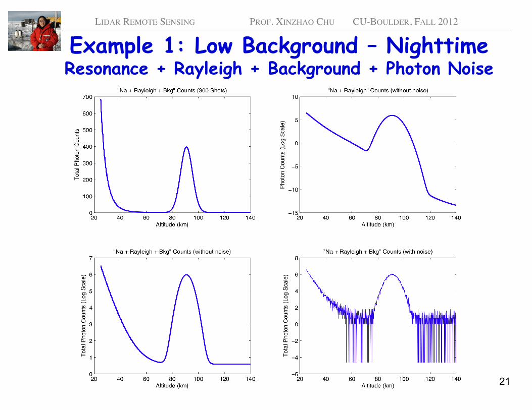
Example 1: Low Background – Nighttime Resonance + Rayleigh + Background + Photon Noise

21


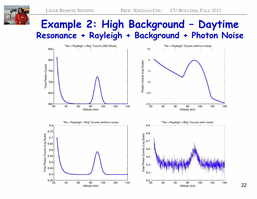
Example 2: High Background – Daytime Resonance + Rayleigh + Background + Photon Noise

22


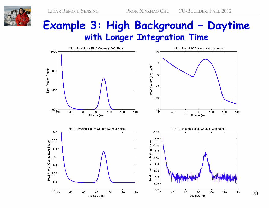
Example 3: High Background – Daytime with Longer Integration Time

23


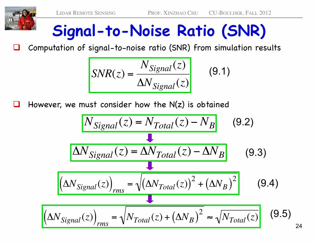
Signal-to-Noise Ratio (SNR)   Computation of signal-to-noise ratio (SNR) from simulation results�

€

SNR(z) =NSignal (z)ΔNSignal (z)

  However, we must consider how the N(z) is obtained�

€

NSignal (z) = NTotal (z) − NB

€

ΔNSignal (z) = ΔNTotal (z) −ΔNB

€

ΔNSignal (z)( )rms = ΔNTotal (z)( )2 + ΔNB( )2

€

ΔNSignal (z)( )rms = NTotal (z) + ΔNB( )2 ≈ NTotal (z)24

(9.1)

(9.2)

(9.3)

(9.4)

(9.5)


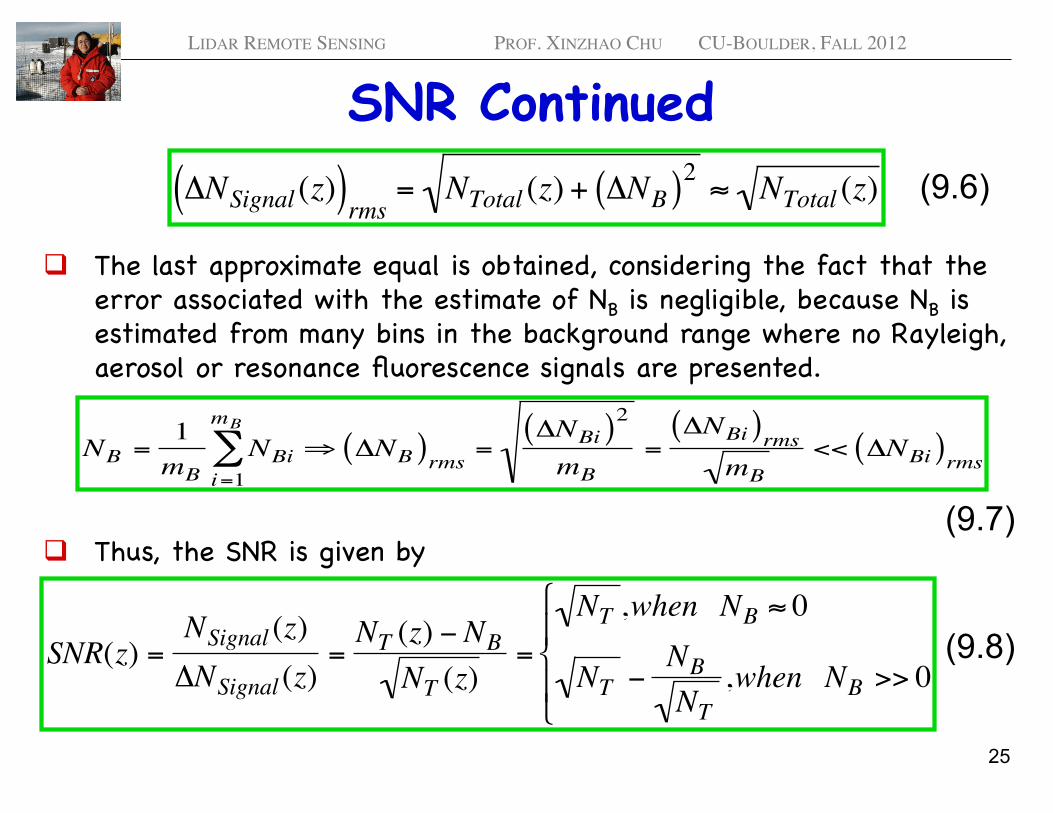
SNR Continued

  The last approximate equal is obtained, considering the fact that the error associated with the estimate of NB is negligible, because NB is estimated from many bins in the background range where no Rayleigh, aerosol or resonance fluorescence signals are presented.�

  Thus, the SNR is given by�

€

ΔNSignal (z)( )rms = NTotal (z) + ΔNB( )2 ≈ NTotal (z)

25

€

SNR(z) =NSignal (z)ΔNSignal (z)

=NT (z) − NB

NT (z)=

NT ,when NB ≈ 0

NT −NBNT

,when NB >> 0

⎧

⎨ ⎪

⎩ ⎪

€

NB =1mB

NBii=1

mB

∑ ⇒ ΔNB( )rms =ΔNBi( )2

mB=ΔNBi( )rms

mB<< ΔNBi( )rms

(9.6)

(9.7)

(9.8)


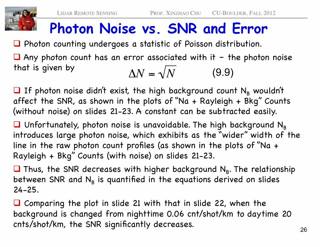
Photon Noise vs. SNR and Error   Photon counting undergoes a statistic of Poisson distribution.�  Any photon count has an error associated with it – the photon noise that is given by�

€

ΔN = N

26

  If photon noise didn’t exist, the high background count NB wouldn’t affect the SNR, as shown in the plots of “Na + Rayleigh + Bkg” Counts (without noise) on slides 21-23. A constant can be subtracted easily.�  Unfortunately, photon noise is unavoidable. The high background NB introduces large photon noise, which exhibits as the “wider” width of the line in the raw photon count profiles (as shown in the plots of “Na + Rayleigh + Bkg” Counts (with noise) on slides 21-23.�  Thus, the SNR decreases with higher background NB. The relationship between SNR and NB is quantified in the equations derived on slides 24-25.�  Comparing the plot in slide 21 with that in slide 22, when the background is changed from nighttime 0.06 cnt/shot/km to daytime 20 cnts/shot/km, the SNR significantly decreases.�

(9.9)


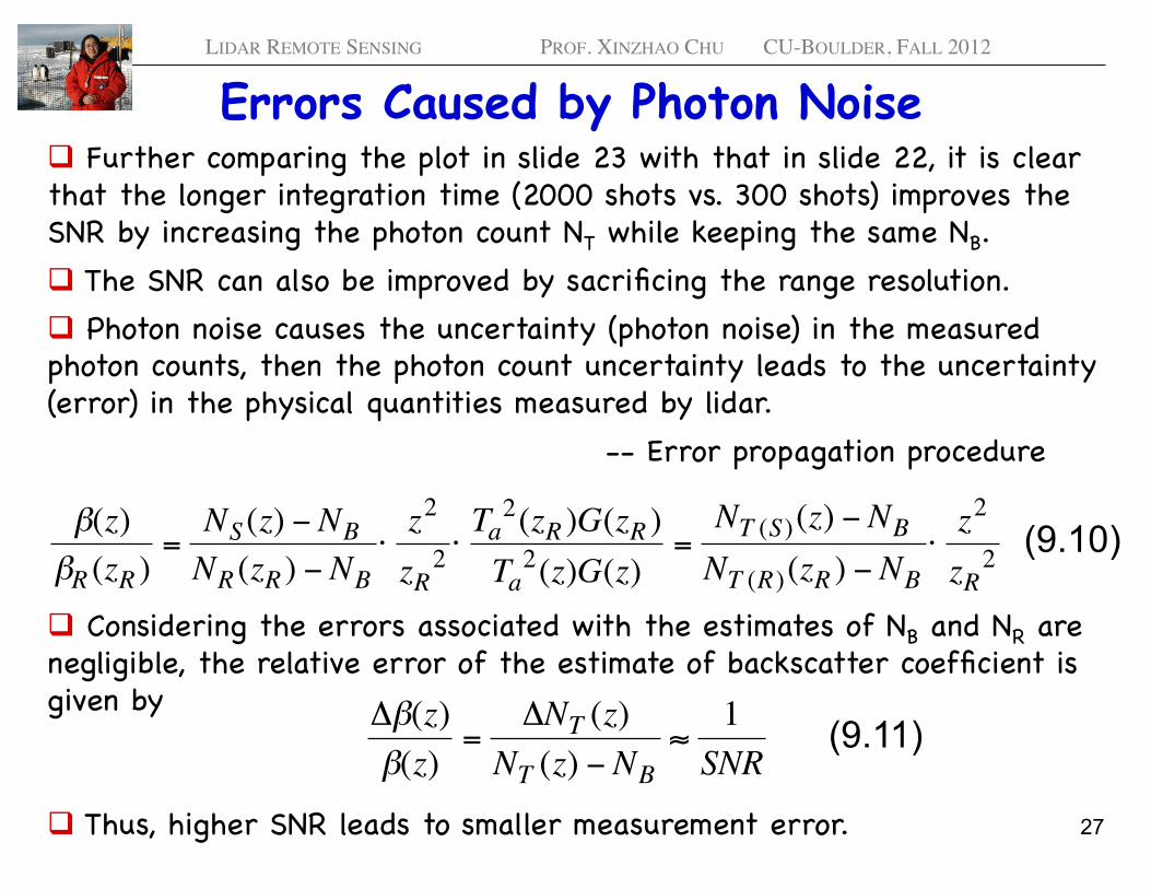
Errors Caused by Photon Noise   Further comparing the plot in slide 23 with that in slide 22, it is clear that the longer integration time (2000 shots vs. 300 shots) improves the SNR by increasing the photon count NT while keeping the same NB. �  The SNR can also be improved by sacrificing the range resolution.�  Photon noise causes the uncertainty (photon noise) in the measured photon counts, then the photon count uncertainty leads to the uncertainty (error) in the physical quantities measured by lidar.�

" " " " "-- Error propagation procedure�

€

β(z)βR (zR )

=NS (z) − NBNR (zR ) − NB

⋅z2

zR2 ⋅Ta2(zR )G(zR )Ta2(z)G(z)

=NT (S)(z) − NBNT (R)(zR ) − NB

⋅z2

zR2

€

Δβ(z)β(z)

=ΔNT (z)

NT (z) − NB≈

1SNR

27

  Considering the errors associated with the estimates of NB and NR are negligible, the relative error of the estimate of backscatter coefficient is given by �

  Thus, higher SNR leads to smaller measurement error.�

(9.10)

(9.11)


Summary   Lidar simulation and error analysis are an integral of our understanding of lidar principle, technology and actual application procedure. �

  It provides a model to investigate how the lidar returns depend on the lidar detection procedure, and how measurement accuracy, precision, and resolution depend on various parameters.�

  It can be used to verify lidar return shapes, assess lidar potentials, guide lidar design and instrumentation, test data retrieval code and metrics, etc.�

  A complete lidar simulation and error analysis code is very complicated. We will go step by step to achieve it.�

28

Download - IDAR , F 2012 Lecture 09. Lidar Simulation and Error ...superlidar.colorado.edu/.../LidarLecture09_LidarSimulation.pdf · Lecture 09. Lidar Simulation ... lidar simulation code complete

Top Related