Download - GLM Theory
15 GeneralizedLinear Models
Due originally to Nelder and Wedderburn (1972), generalized linear models are a remarkablesynthesis and extension of familiar regression models such as the linear models described in
Part II of this text and the logit and probit models described in the preceding chapter. The currentchapter begins with a consideration of the general structure and range of application of generalizedlinear models; proceeds to examine in greater detail generalized linear models for count data,including contingency tables; briefly sketches the statistical theory underlying generalized linearmodels; and concludes with the extension of regression diagnostics to generalized linear models.
The unstarred sections of this chapter are perhaps more difficult than the unstarred material inpreceding chapters. Generalized linear models have become so central to effective statistical dataanalysis, however, that it is worth the additional effort required to acquire a basic understandingof the subject.
15.1 The Structure of Generalized Linear Models
A generalized linear model (or GLM1) consists of three components:
1. A random component, specifying the conditional distribution of the response variable, Yi(for the ith of n independently sampled observations), given the values of the explanatoryvariables in the model. In Nelder and Wedderburn’s original formulation, the distributionof Yi is a member of an exponential family, such as the Gaussian (normal), binomial, Pois-son, gamma, or inverse-Gaussian families of distributions. Subsequent work, however, hasextended GLMs to multivariate exponential families (such as the multinomial distribution),to certain non-exponential families (such as the two-parameter negative-binomial distribu-tion), and to some situations in which the distribution of Yi is not specified completely.Most of these ideas are developed later in the chapter.
2. A linear predictor—that is a linear function of regressors
ηi = α + β1Xi1 + β2Xi2 + · · · + βkXik
As in the linear model, and in the logit and probit models of Chapter 14, the regressorsXij areprespecified functions of the explanatory variables and therefore may include quantitativeexplanatory variables, transformations of quantitative explanatory variables, polynomialregressors, dummy regressors, interactions, and so on. Indeed, one of the advantages ofGLMs is that the structure of the linear predictor is the familiar structure of a linear model.
3. A smooth and invertible linearizing link function g(·), which transforms the expectation ofthe response variable, μi ≡ E(Yi), to the linear predictor:
g(μi) = ηi = α + β1Xi1 + β2Xi2 + · · · + βkXik
1Some authors use the acronym “GLM” to refer to the “general linear model”—that is, the linear regression model withnormal errors described in Part II of the text—and instead employ “GLIM” to denote generalized linear models (whichis also the name of a computer program used to fit GLMs).
379
380 Chapter 15. Generalized Linear Models
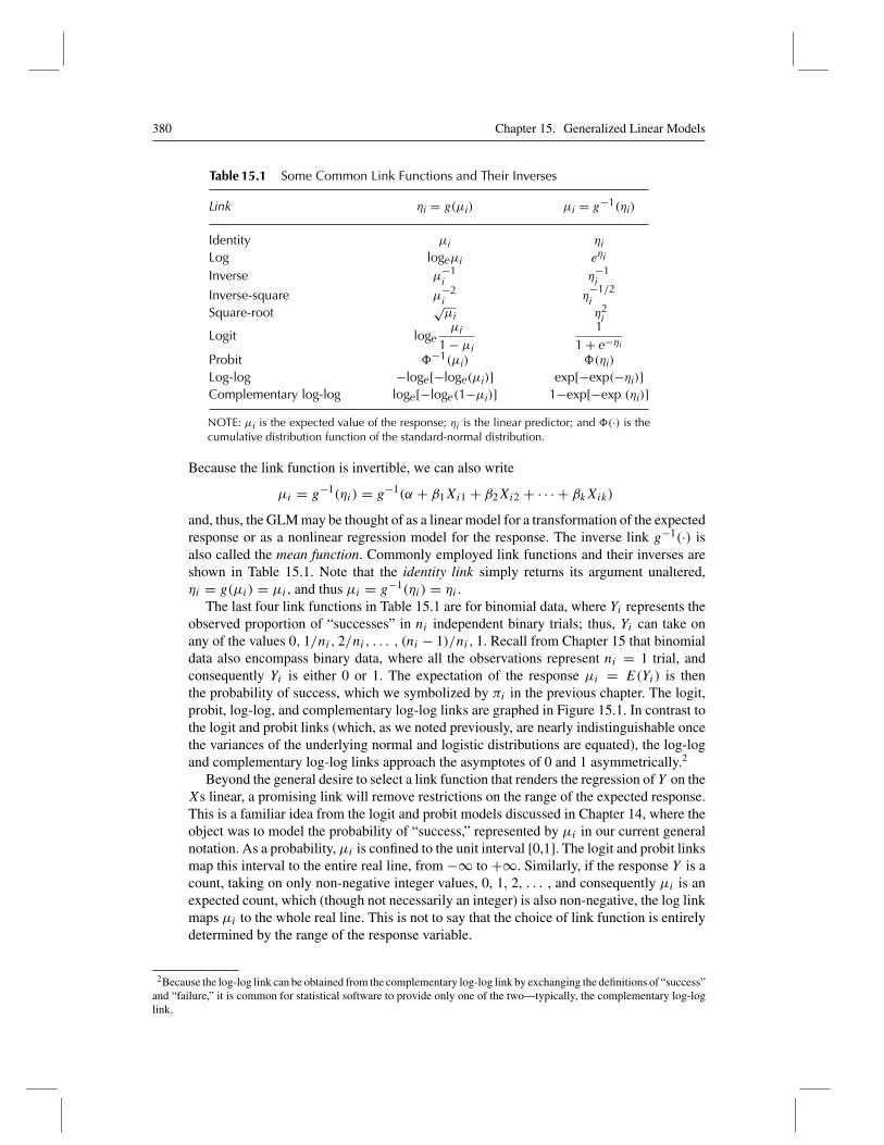
Table 15.1 Some Common Link Functions and Their Inverses
Link ηi = g(μi) μi = g−1(ηi)
Identity μi ηiLog logeμi eηi
Inverse μ−1i η−1
iInverse-square μ−2
i η−1/2i
Square-root√μi η2
i
Logit logeμi
1 − μi
11 + e−ηi
Probit �−1(μi) �(ηi)
Log-log −loge[−loge(μi)] exp[−exp(−ηi)]Complementary log-log loge[−loge(1−μi)] 1−exp[−exp (ηi)]
NOTE: μi is the expected value of the response; ηi is the linear predictor; and �(·) is thecumulative distribution function of the standard-normal distribution.
Because the link function is invertible, we can also write
μi = g−1(ηi) = g−1(α + β1Xi1 + β2Xi2 + · · · + βkXik)
and, thus, the GLM may be thought of as a linear model for a transformation of the expectedresponse or as a nonlinear regression model for the response. The inverse link g−1(·) isalso called the mean function. Commonly employed link functions and their inverses areshown in Table 15.1. Note that the identity link simply returns its argument unaltered,ηi = g(μi) = μi , and thus μi = g−1(ηi) = ηi .
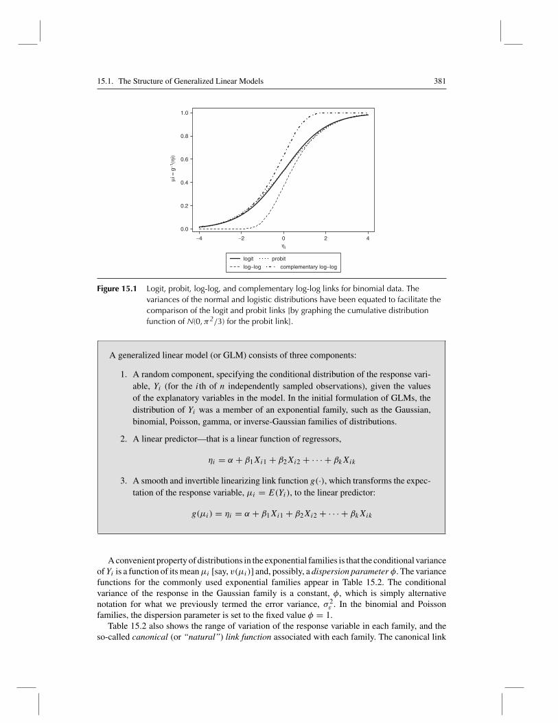
The last four link functions in Table 15.1 are for binomial data, where Yi represents theobserved proportion of “successes” in ni independent binary trials; thus, Yi can take onany of the values 0, 1/ni, 2/ni, . . . , (ni − 1)/ni, 1. Recall from Chapter 15 that binomialdata also encompass binary data, where all the observations represent ni = 1 trial, andconsequently Yi is either 0 or 1. The expectation of the response μi = E(Yi) is thenthe probability of success, which we symbolized by πi in the previous chapter. The logit,probit, log-log, and complementary log-log links are graphed in Figure 15.1. In contrast tothe logit and probit links (which, as we noted previously, are nearly indistinguishable oncethe variances of the underlying normal and logistic distributions are equated), the log-logand complementary log-log links approach the asymptotes of 0 and 1 asymmetrically.2
Beyond the general desire to select a link function that renders the regression of Y on theXs linear, a promising link will remove restrictions on the range of the expected response.This is a familiar idea from the logit and probit models discussed in Chapter 14, where theobject was to model the probability of “success,” represented by μi in our current generalnotation. As a probability, μi is confined to the unit interval [0,1]. The logit and probit linksmap this interval to the entire real line, from −∞ to +∞. Similarly, if the response Y is acount, taking on only non-negative integer values, 0, 1, 2, . . . , and consequently μi is anexpected count, which (though not necessarily an integer) is also non-negative, the log linkmaps μi to the whole real line. This is not to say that the choice of link function is entirelydetermined by the range of the response variable.
2Because the log-log link can be obtained from the complementary log-log link by exchanging the definitions of “success”and “failure,” it is common for statistical software to provide only one of the two—typically, the complementary log-loglink.
15.1. The Structure of Generalized Linear Models 381
−4 −2 0 2 4
0.0
0.2
0.4
0.6
0.8
1.0
ηi
logit probit
log–log complementary log–log
μi =
g−1
(ηi)
Figure 15.1 Logit, probit, log-log, and complementary log-log links for binomial data. Thevariances of the normal and logistic distributions have been equated to facilitate thecomparison of the logit and probit links [by graphing the cumulative distributionfunction of N(0,π2/3) for the probit link].
A generalized linear model (or GLM) consists of three components:
1. A random component, specifying the conditional distribution of the response vari-able, Yi (for the ith of n independently sampled observations), given the valuesof the explanatory variables in the model. In the initial formulation of GLMs, thedistribution of Yi was a member of an exponential family, such as the Gaussian,binomial, Poisson, gamma, or inverse-Gaussian families of distributions.
2. A linear predictor—that is a linear function of regressors,
ηi = α + β1Xi1 + β2Xi2 + · · · + βkXik
3. A smooth and invertible linearizing link function g(·), which transforms the expec-tation of the response variable, μi = E(Yi), to the linear predictor:
g(μi) = ηi = α + β1Xi1 + β2Xi2 + · · · + βkXik
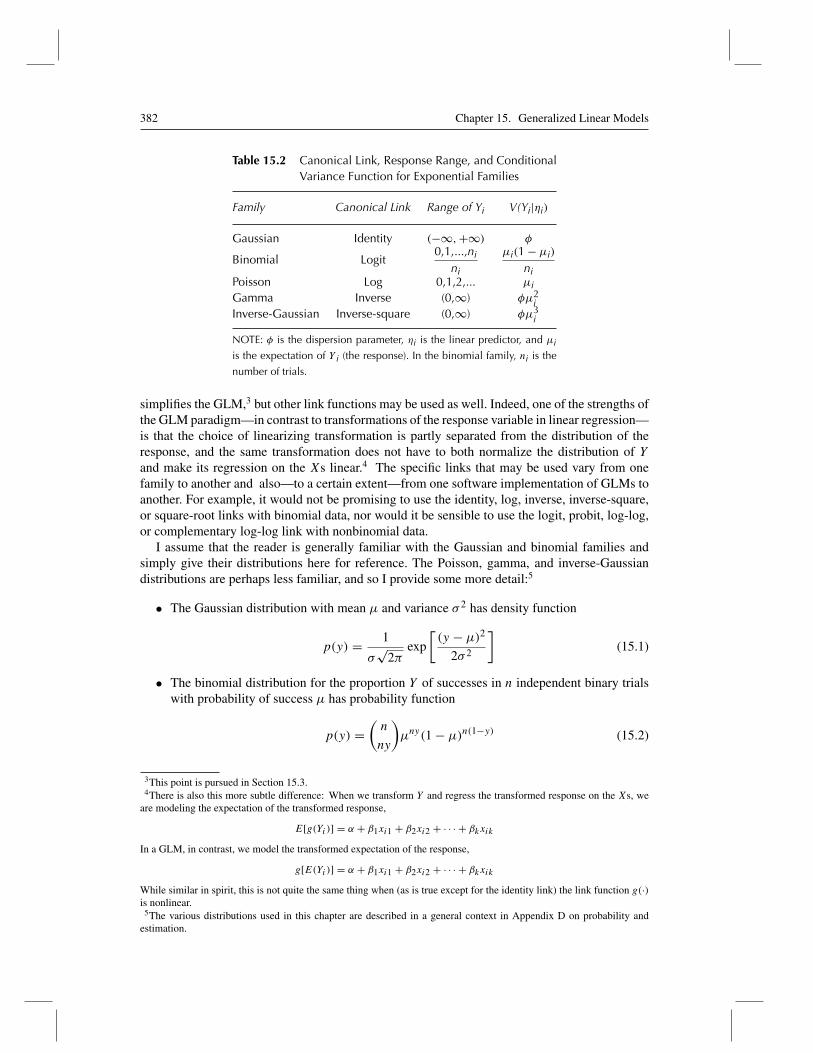
A convenient property of distributions in the exponential families is that the conditional varianceofYi is a function of its meanμi [say, v(μi)] and, possibly, a dispersion parameter φ. The variancefunctions for the commonly used exponential families appear in Table 15.2. The conditionalvariance of the response in the Gaussian family is a constant, φ, which is simply alternativenotation for what we previously termed the error variance, σ 2
ε . In the binomial and Poissonfamilies, the dispersion parameter is set to the fixed value φ = 1.
Table 15.2 also shows the range of variation of the response variable in each family, and theso-called canonical (or “natural”) link function associated with each family. The canonical link
382 Chapter 15. Generalized Linear Models
Table 15.2 Canonical Link, Response Range, and ConditionalVariance Function for Exponential Families
Family Canonical Link Range of Yi V(Yi|ηi)
Gaussian Identity (−∞,+∞) φ
Binomial Logit0,1,...,ni
ni
μi(1 − μi)
niPoisson Log 0,1,2,... μiGamma Inverse (0,∞) φμ2
iInverse-Gaussian Inverse-square (0,∞) φμ3
i
NOTE: φ is the dispersion parameter, ηi is the linear predictor, and μiis the expectation of Y i (the response). In the binomial family, ni is the
number of trials.
simplifies the GLM,3 but other link functions may be used as well. Indeed, one of the strengths ofthe GLM paradigm—in contrast to transformations of the response variable in linear regression—is that the choice of linearizing transformation is partly separated from the distribution of theresponse, and the same transformation does not have to both normalize the distribution of Yand make its regression on the Xs linear.4 The specific links that may be used vary from onefamily to another and also—to a certain extent—from one software implementation of GLMs toanother. For example, it would not be promising to use the identity, log, inverse, inverse-square,or square-root links with binomial data, nor would it be sensible to use the logit, probit, log-log,or complementary log-log link with nonbinomial data.
I assume that the reader is generally familiar with the Gaussian and binomial families andsimply give their distributions here for reference. The Poisson, gamma, and inverse-Gaussiandistributions are perhaps less familiar, and so I provide some more detail:5
• The Gaussian distribution with mean μ and variance σ 2 has density function
p(y) = 1
σ√
2πexp
[(y − μ)2
2σ 2
](15.1)
• The binomial distribution for the proportion Y of successes in n independent binary trialswith probability of success μ has probability function
p(y) =(n
ny
)μny(1 − μ)n(1−y) (15.2)
3This point is pursued in Section 15.3.4There is also this more subtle difference: When we transform Y and regress the transformed response on the Xs, we
are modeling the expectation of the transformed response,
E[g(Yi )] = α + β1xi1 + β2xi2 + · · · + βkxik
In a GLM, in contrast, we model the transformed expectation of the response,
g[E(Yi)] = α + β1xi1 + β2xi2 + · · · + βkxik
While similar in spirit, this is not quite the same thing when (as is true except for the identity link) the link function g(·)is nonlinear.
5The various distributions used in this chapter are described in a general context in Appendix D on probability andestimation.
15.1. The Structure of Generalized Linear Models 383
Here, ny is the observed number of successes in the n trials, and n(1 − y) is the number offailures; and (
n
ny
)= n!
(ny)![n(1 − y)]!
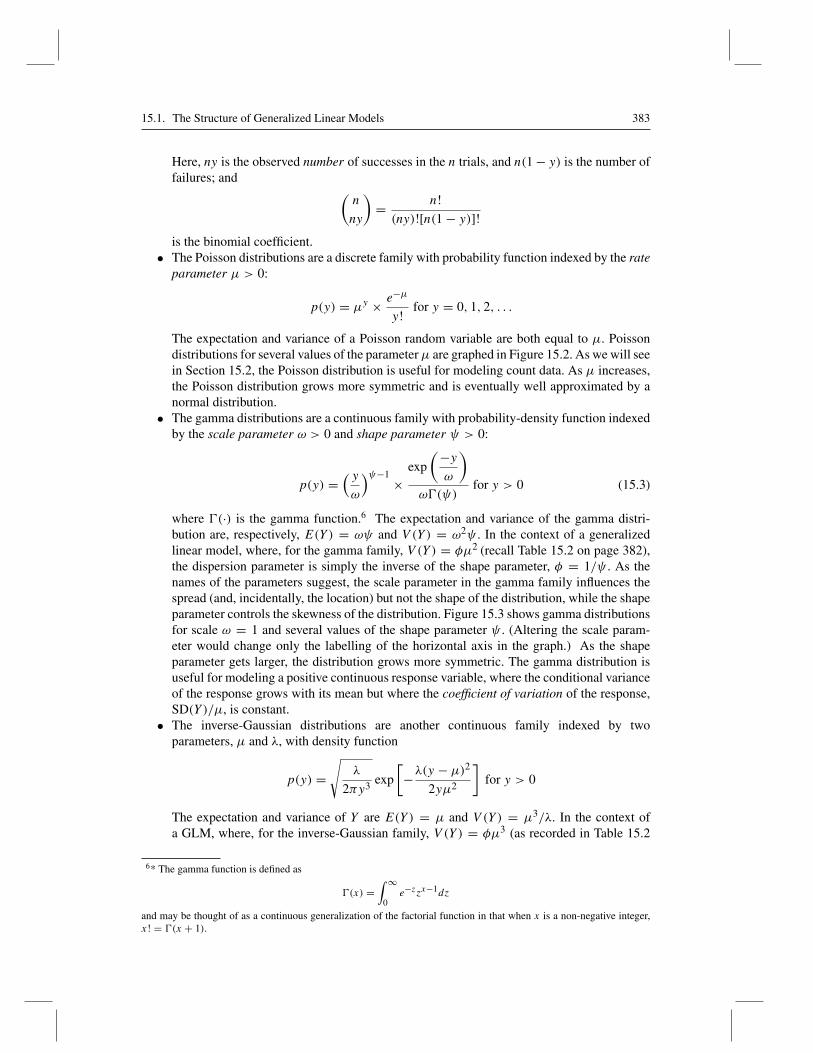
is the binomial coefficient.• The Poisson distributions are a discrete family with probability function indexed by the rate
parameter μ > 0:
p(y) = μy × e−μ
y!for y = 0, 1, 2, . . .
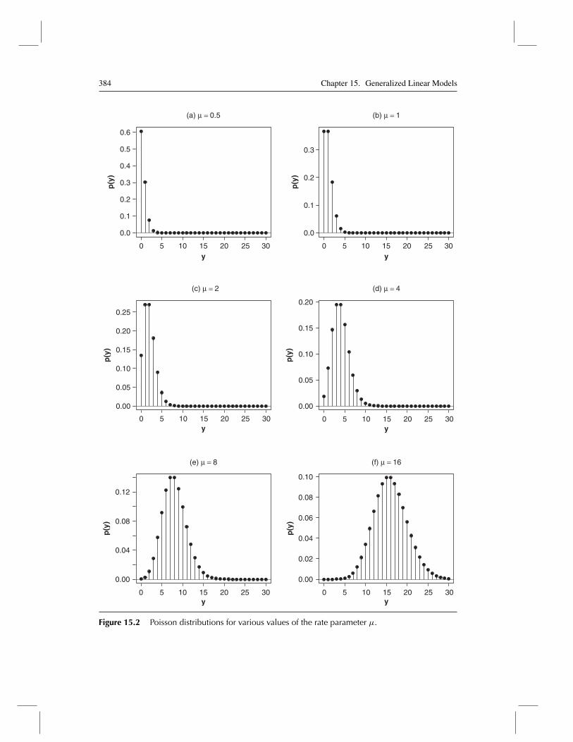
The expectation and variance of a Poisson random variable are both equal to μ. Poissondistributions for several values of the parameterμ are graphed in Figure 15.2. As we will seein Section 15.2, the Poisson distribution is useful for modeling count data. As μ increases,the Poisson distribution grows more symmetric and is eventually well approximated by anormal distribution.
• The gamma distributions are a continuous family with probability-density function indexedby the scale parameter ω > 0 and shape parameter ψ > 0:
p(y) =( yω
)ψ−1 ×exp
(−yω
)ω�(ψ)
for y > 0 (15.3)
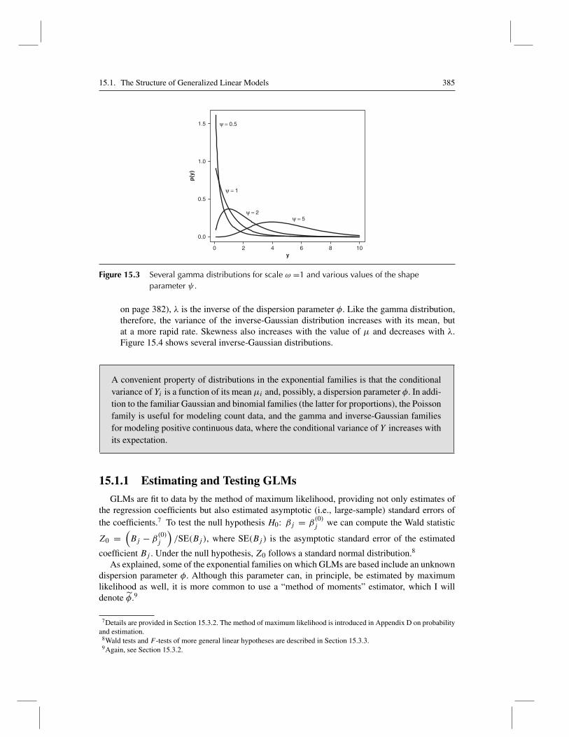
where �(·) is the gamma function.6 The expectation and variance of the gamma distri-bution are, respectively, E(Y ) = ωψ and V (Y ) = ω2ψ . In the context of a generalizedlinear model, where, for the gamma family, V (Y ) = φμ2 (recall Table 15.2 on page 382),the dispersion parameter is simply the inverse of the shape parameter, φ = 1/ψ . As thenames of the parameters suggest, the scale parameter in the gamma family influences thespread (and, incidentally, the location) but not the shape of the distribution, while the shapeparameter controls the skewness of the distribution. Figure 15.3 shows gamma distributionsfor scale ω = 1 and several values of the shape parameter ψ . (Altering the scale param-eter would change only the labelling of the horizontal axis in the graph.) As the shapeparameter gets larger, the distribution grows more symmetric. The gamma distribution isuseful for modeling a positive continuous response variable, where the conditional varianceof the response grows with its mean but where the coefficient of variation of the response,SD(Y )/μ, is constant.
• The inverse-Gaussian distributions are another continuous family indexed by twoparameters, μ and λ, with density function
p(y) =√
λ
2πy3exp
[−λ(y − μ)2
2yμ2
]for y > 0
The expectation and variance of Y are E(Y ) = μ and V (Y ) = μ3/λ. In the context ofa GLM, where, for the inverse-Gaussian family, V (Y ) = φμ3 (as recorded in Table 15.2
6* The gamma function is defined as
�(x) =∫ ∞
0e−zzx−1dz
and may be thought of as a continuous generalization of the factorial function in that when x is a non-negative integer,x! = �(x + 1).
384 Chapter 15. Generalized Linear Models
0 10 15 20 25 30y
p(y
)
y
p(y
)
0 10 15 20 25 30y
p(y
)
0 10 15 20 25 30y
p(y
)
0 10 15 20 25 30y
p(y
)
0 10 15 20 25 30y
p(y
)
0.6
0.5
0.4
0.3
0.2
0.1
0.0
(a) μ = 0.5 (b) μ = 1
5 0 10 15 20 25 305
0.3
0.0
0.1
0.2
(c) μ = 2 (d) μ = 4
0.25
0.20
0.15
0.10
0.05
0.00
5
0.20
0.15
0.10
0.05
0.00
5
(e) μ = 8 (f) μ = 16
0.12
0.08
0.04
0.00
5
0.10
0.08
0.06
0.04
0.02
0.00
5
Figure 15.2 Poisson distributions for various values of the rate parameter μ.
15.1. The Structure of Generalized Linear Models 385
0 2 4 6 8 10y
p(y
)
ψ = 2ψ = 5
ψ = 1
ψ = 0.51.5
1.0
0.5
0.0
Figure 15.3 Several gamma distributions for scale ω =1 and various values of the shapeparameter ψ .
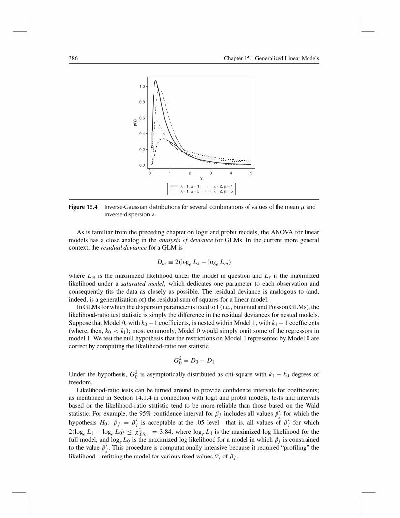
on page 382), λ is the inverse of the dispersion parameter φ. Like the gamma distribution,therefore, the variance of the inverse-Gaussian distribution increases with its mean, butat a more rapid rate. Skewness also increases with the value of μ and decreases with λ.Figure 15.4 shows several inverse-Gaussian distributions.
A convenient property of distributions in the exponential families is that the conditionalvariance of Yi is a function of its mean μi and, possibly, a dispersion parameter φ. In addi-tion to the familiar Gaussian and binomial families (the latter for proportions), the Poissonfamily is useful for modeling count data, and the gamma and inverse-Gaussian familiesfor modeling positive continuous data, where the conditional variance of Y increases withits expectation.
15.1.1 Estimating and Testing GLMs
GLMs are fit to data by the method of maximum likelihood, providing not only estimates ofthe regression coefficients but also estimated asymptotic (i.e., large-sample) standard errors ofthe coefficients.7 To test the null hypothesis H0: βj = β
(0)j we can compute the Wald statistic
Z0 =(Bj − β
(0)j
)/SE(Bj ), where SE(Bj ) is the asymptotic standard error of the estimated
coefficient Bj . Under the null hypothesis, Z0 follows a standard normal distribution.8
As explained, some of the exponential families on which GLMs are based include an unknowndispersion parameter φ. Although this parameter can, in principle, be estimated by maximumlikelihood as well, it is more common to use a “method of moments” estimator, which I willdenote φ.9
7Details are provided in Section 15.3.2. The method of maximum likelihood is introduced in Appendix D on probabilityand estimation.
8Wald tests and F -tests of more general linear hypotheses are described in Section 15.3.3.9Again, see Section 15.3.2.
386 Chapter 15. Generalized Linear Models
0 1 2 3 4 5y
p(y
)
1.0
0.8
0.6
0.4
0.2
0.0
λ = 1, μ = 1 λ = 2, μ = 1λ = 1, μ = 5 λ = 2, μ = 5
Figure 15.4 Inverse-Gaussian distributions for several combinations of values of the mean μ andinverse-dispersion λ.
As is familiar from the preceding chapter on logit and probit models, the ANOVA for linearmodels has a close analog in the analysis of deviance for GLMs. In the current more generalcontext, the residual deviance for a GLM is
Dm ≡ 2(loge Ls − loge Lm)
where Lm is the maximized likelihood under the model in question and Ls is the maximizedlikelihood under a saturated model, which dedicates one parameter to each observation andconsequently fits the data as closely as possible. The residual deviance is analogous to (and,indeed, is a generalization of) the residual sum of squares for a linear model.
In GLMs for which the dispersion parameter is fixed to 1 (i.e., binomial and Poisson GLMs), thelikelihood-ratio test statistic is simply the difference in the residual deviances for nested models.Suppose that Model 0, with k0 + 1 coefficients, is nested within Model 1, with k1 + 1 coefficients(where, then, k0 < k1); most commonly, Model 0 would simply omit some of the regressors inmodel 1. We test the null hypothesis that the restrictions on Model 1 represented by Model 0 arecorrect by computing the likelihood-ratio test statistic
G20 = D0 −D1
Under the hypothesis, G20 is asymptotically distributed as chi-square with k1 − k0 degrees of
freedom.Likelihood-ratio tests can be turned around to provide confidence intervals for coefficients;
as mentioned in Section 14.1.4 in connection with logit and probit models, tests and intervalsbased on the likelihood-ratio statistic tend to be more reliable than those based on the Waldstatistic. For example, the 95% confidence interval for βj includes all values β ′
j for which thehypothesis H0: βj = β ′
j is acceptable at the .05 level—that is, all values of β ′j for which
2(loge L1 − loge L0) ≤ χ2.05,1 = 3.84, where loge L1 is the maximized log likelihood for the
full model, and loge L0 is the maximized log likelihood for a model in which βj is constrainedto the value β ′
j . This procedure is computationally intensive because it required “profiling” thelikelihood—refitting the model for various fixed values β ′
j of βj .
15.2. Generalized Linear Models for Counts 387
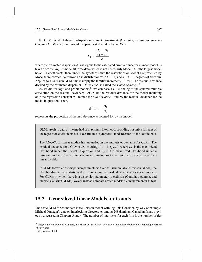
For GLMs in which there is a dispersion parameter to estimate (Gaussian, gamma, and inverse-Gaussian GLMs), we can instead compare nested models by an F -test,
F0 =D0 −D1
k1 − k0
φ
where the estimated dispersion φ, analogous to the estimated error variance for a linear model, istaken from the largest model fit to the data (which is not necessarily Model 1). If the largest modelhas k + 1 coefficients, then, under the hypothesis that the restrictions on Model 1 represented byModel 0 are correct, F0 follows an F -distribution with k1 − k0 and n− k− 1 degrees of freedom.Applied to a Gaussian GLM, this is simply the familiar incremental F -test. The residual deviancedivided by the estimated dispersion, D∗ ≡ D/φ, is called the scaled deviance.10
As we did for logit and probit models,11 we can base a GLM analog of the squared multiplecorrelation on the residual deviance: Let D0 be the residual deviance for the model includingonly the regression constant α—termed the null deviance—and D1 the residual deviance for themodel in question. Then,
R2 ≡ 1 − D1
D0
represents the proportion of the null deviance accounted for by the model.
GLMs are fit to data by the method of maximum likelihood, providing not only estimates ofthe regression coefficients but also estimated asymptotic standard errors of the coefficients.
The ANOVA for linear models has an analog in the analysis of deviance for GLMs. Theresidual deviance for a GLM is Dm = 2(loge Ls − loge Lm), where Lm is the maximizedlikelihood under the model in question and Ls is the maximized likelihood under asaturated model. The residual deviance is analogous to the residual sum of squares for alinear model.
In GLMs for which the dispersion parameter is fixed to 1 (binomial and Poisson GLMs), thelikelihood-ratio test statistic is the difference in the residual deviances for nested models.For GLMs in which there is a dispersion parameter to estimate (Gaussian, gamma, andinverse-Gaussian GLMs), we can instead compare nested models by an incrementalF -test.
15.2 Generalized Linear Models for Counts
The basic GLM for count data is the Poisson model with log link. Consider, by way of example,Michael Ornstein’s data on interlocking directorates among 248 dominant Canadian firms, previ-ously discussed in Chapters 3 and 4. The number of interlocks for each firm is the number of ties
10Usage is not entirely uniform here, and either of the residual deviance or the scaled deviance is often simply termed“the deviance.”11See Section 14.1.4.
388 Chapter 15. Generalized Linear Models
0 20 40 60 80 100
Number of Interlocks
Fre
qu
ency
25
20
15
10
5
0
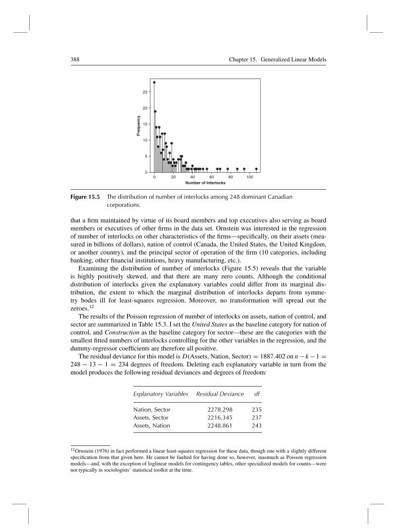
Figure 15.5 The distribution of number of interlocks among 248 dominant Canadiancorporations.
that a firm maintained by virtue of its board members and top executives also serving as boardmembers or executives of other firms in the data set. Ornstein was interested in the regressionof number of interlocks on other characteristics of the firms—specifically, on their assets (mea-sured in billions of dollars), nation of control (Canada, the United States, the United Kingdom,or another country), and the principal sector of operation of the firm (10 categories, includingbanking, other financial institutions, heavy manufacturing, etc.).
Examining the distribution of number of interlocks (Figure 15.5) reveals that the variableis highly positively skewed, and that there are many zero counts. Although the conditionaldistribution of interlocks given the explanatory variables could differ from its marginal dis-tribution, the extent to which the marginal distribution of interlocks departs from symme-try bodes ill for least-squares regression. Moreover, no transformation will spread out thezeroes.12
The results of the Poisson regression of number of interlocks on assets, nation of control, andsector are summarized in Table 15.3. I set the United States as the baseline category for nation ofcontrol, and Construction as the baseline category for sector—these are the categories with thesmallest fitted numbers of interlocks controlling for the other variables in the regression, and thedummy-regressor coefficients are therefore all positive.
The residual deviance for this model isD(Assets, Nation, Sector) = 1887.402 on n− k−1 =248 − 13 − 1 = 234 degrees of freedom. Deleting each explanatory variable in turn from themodel produces the following residual deviances and degrees of freedom:
Explanatory Variables Residual Deviance df
Nation, Sector 2278.298 235Assets, Sector 2216.345 237Assets, Nation 2248.861 243
12Ornstein (1976) in fact performed a linear least-squares regression for these data, though one with a slightly differentspecification from that given here. He cannot be faulted for having done so, however, inasmuch as Poisson regressionmodels—and, with the exception of loglinear models for contingency tables, other specialized models for counts—werenot typically in sociologists’ statistical toolkit at the time.
15.2. Generalized Linear Models for Counts 389
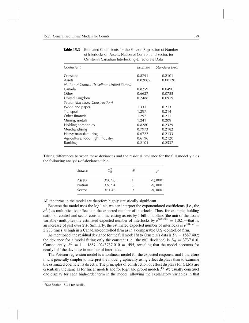
Table 15.3 Estimated Coefficients for the Poisson Regression of Numberof Interlocks on Assets, Nation of Control, and Sector, forOrnstein’s Canadian Interlocking-Directorate Data
Coefficient Estimate Standard Error
Constant 0.8791 0.2101Assets 0.02085 0.00120Nation of Control (baseline: United States)Canada 0.8259 0.0490Other 0.6627 0.0755United Kingdom 0.2488 0.0919Sector (Baseline: Construction)Wood and paper 1.331 0.213Transport 1.297 0.214Other financial 1.297 0.211Mining, metals 1.241 0.209Holding companies 0.8280 0.2329Merchandising 0.7973 0.2182Heavy manufacturing 0.6722 0.2133Agriculture, food, light industry 0.6196 0.2120Banking 0.2104 0.2537
Taking differences between these deviances and the residual deviance for the full model yieldsthe following analysis-of-deviance table:
Source G20 df p
Assets 390.90 1 �.0001Nation 328.94 3 �.0001Sector 361.46 9 �.0001
All the terms in the model are therefore highly statistically significant.Because the model uses the log link, we can interpret the exponentiated coefficients (i.e., the
eBj ) as multiplicative effects on the expected number of interlocks. Thus, for example, holdingnation of control and sector constant, increasing assets by 1 billion dollars (the unit of the assetsvariable) multiplies the estimated expected number of interlocks by e0.02085 = 1.021—that is,an increase of just over 2%. Similarly, the estimated expected number of interlocks is e0.8259 =2.283 times as high in a Canadian-controlled firm as in a comparable U.S.-controlled firm.
As mentioned, the residual deviance for the full model fit to Ornstein’s data isD1 = 1887.402;the deviance for a model fitting only the constant (i.e., the null deviance) is D0 = 3737.010.Consequently, R2 = 1 − 1887.402/3737.010 = .495, revealing that the model accounts fornearly half the deviance in number of interlocks.
The Poisson-regression model is a nonlinear model for the expected response, and I thereforefind it generally simpler to interpret the model graphically using effect displays than to examinethe estimated coefficients directly. The principles of construction of effect displays for GLMs areessentially the same as for linear models and for logit and probit models:13 We usually constructone display for each high-order term in the model, allowing the explanatory variables in that
13See Section 15.3.4 for details.
390 Chapter 15. Generalized Linear Models
0 50 100 150
1
2
3
4
5
6
(a)
Assets (billions of dollars)
24816
64
256
Nu
mb
er o
f In
terl
ock
s
Nu
mb
er o
f In
terl
ock
s
Nu
mb
er o
f In
terl
ock
s
(b)
Nation of Control
Canada Other U.S. U.K.
12
3
4
5
6
24816
64
256
(c)
SectorWOD TRN FIN MIN HLD MER MAN AGR BNK CON
1
2
3
4
5
6
24816
64
256
log
eNu
mb
er o
f In
terl
ock
s
log
eNu
mb
er o
f In
terl
ock
s
log
eNu
mb
er o
f In
terl
ock
s
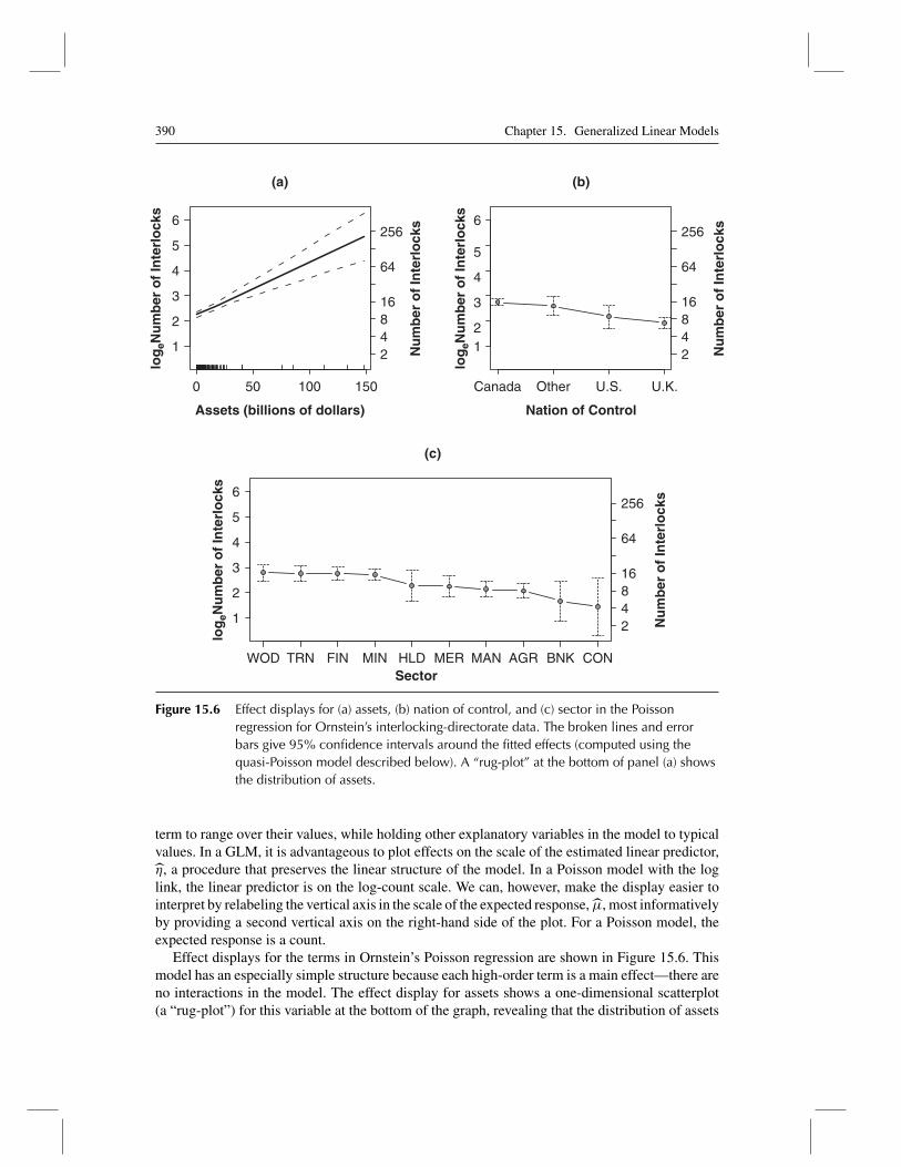
Figure 15.6 Effect displays for (a) assets, (b) nation of control, and (c) sector in the Poissonregression for Ornstein’s interlocking-directorate data. The broken lines and errorbars give 95% confidence intervals around the fitted effects (computed using thequasi-Poisson model described below). A “rug-plot” at the bottom of panel (a) showsthe distribution of assets.
term to range over their values, while holding other explanatory variables in the model to typicalvalues. In a GLM, it is advantageous to plot effects on the scale of the estimated linear predictor,η, a procedure that preserves the linear structure of the model. In a Poisson model with the loglink, the linear predictor is on the log-count scale. We can, however, make the display easier tointerpret by relabeling the vertical axis in the scale of the expected response, μ, most informativelyby providing a second vertical axis on the right-hand side of the plot. For a Poisson model, theexpected response is a count.
Effect displays for the terms in Ornstein’s Poisson regression are shown in Figure 15.6. Thismodel has an especially simple structure because each high-order term is a main effect—there areno interactions in the model. The effect display for assets shows a one-dimensional scatterplot(a “rug-plot”) for this variable at the bottom of the graph, revealing that the distribution of assets
15.2. Generalized Linear Models for Counts 391
is highly skewed to the right. Skewness produces some high-leverage observations and suggeststhe possibility of a nonlinear effect for assets, points that I pursue later in the chapter.14
15.2.1 Models for Overdispersed Count Data
The residual deviance for the Poisson regression model fit to the interlocking-directorate data,D = 1887.4, is much larger than the 234 residual degrees of freedom for the model. If the Poissonmodel fits the data reasonably, we would expect the residual deviance to be roughly equal to theresidual degrees of freedom.15 That the residual deviance is so large suggests that the conditionalvariation of the expected number of interlocks exceeds the variation of a Poisson-distributedvariable, for which the variance equals the mean. This common occurrence in the analysis ofcount data is termed overdispersion.16 Indeed, overdispersion is so common in regression modelsfor count data, and its consequences are potentially so severe, that models such as the quasi-Poisson and negative-binomial GLMs discussed in this section should be employed as a matterof course.
The Quasi-Poisson Model
A simple remedy for overdispersed count data is to introduce a dispersion parameter into thePoisson model, so that the conditional variance of the response is now V (Yi |ηi) = φμi . If φ > 1,therefore, the conditional variance of Y increases more rapidly than its mean. There is no expo-nential family corresponding to this specification, and the resulting GLM does not imply a specificprobability distribution for the response variable. Rather, the model specifies the conditional meanand variance of Yi directly. Because the model does not give a probability distribution for Yi , itcannot be estimated by maximum likelihood. Nevertheless, the usual procedure for maximum-likelihood estimation of a GLM yields the so-called quasi-likelihood estimators of the regressioncoefficients, which share many of the properties of maximum-likelihood estimators.17
As it turns out, the quasi-likelihood estimates of the regression coefficients are identical to theML estimates for the Poisson model. The estimated coefficient standard errors differ, however:If φ is the estimated dispersion for the model, then the coefficient standard errors for the quasi-Poisson model are φ1/2 times those for the Poisson model. In the event of overdispersion, therefore,where φ > 1, the effect of introducing a dispersion parameter and obtaining quasi-likelihood esti-mates is (realistically) to inflate the coefficient standard errors. Likewise, F -tests for terms in themodel will reflect the estimated dispersion parameter, producing smaller test statistics and largerp-values.
As explained in the following section, we use a method-of-moments estimator for the dispersionparameter. In the quasi-Poisson model, the dispersion estimator takes the form
φ = 1
n− k − 1
∑ (Yi − μi)2
μi
14See Section 15.4 on diagnostics for GLMs.15That is, the ratio of the residual deviance to degrees of freedom can be taken as an estimate of the dispersion parameterφ, which, in a Poisson model, is fixed to 1. It should be noted, however, that this deviance-based estimator of the dispersioncan perform poorly. A generally preferable “method of moments” estimator is given in Section 15.3.16Although it is much less common, it is also possible for count data to be underdispersed—that is, for the conditionalvariation of the response to be less than the mean. The remedy for underdispsered count data is the same as for overdisperseddata; for example, we can fit a quasi-Poisson model with a dispersion parameter, as described immediately below.17See Section 15.3.2.
392 Chapter 15. Generalized Linear Models
where μi = g−1(ηi) is the fitted expectation of Yi . Applied to Ornstein’s interlocking-directorateregression, for example, we get φ = 7.9435, and, therefore, the standard errors of the regressioncoefficients for the Poisson model in Table 15.3 are each multiplied by
√7.9435 = 2.818.
I note in passing that there is a similar quasi-binomial model for over-dispersed proportions,replacing the fixed dispersion parameter of 1 in the binomial distribution with a dispersion param-eter φ to be estimated from the data. Overdispersed binomial data can arise, for example, whendifferent individuals who share the same values of the explanatory variables nevertheless differin their probability μ of success, a situation that is termed unmodelled heterogeneity. Similarly,overdispersion can occur when binomial observations are not independent, as required by thebinomial distribution—for example, when each binomial observation is for related individuals,such as members of a family.
The Negative-Binomial Model
There are several routes to models for counts based on the negative-binomial distribution (see,e.g., Long, 1997, sect. 8.3; McCullagh & Nelder, 1989, sect. 6.2.3). One approach (followingMcCullagh & Nelder, 1989, p. 233) is to adopt a Poisson model for the count Yi but to supposethat the expected count μ∗
i is itself an unobservable random variable that is gamma-distributedwith mean μi and constant scale parameter ω (implying that the the gamma shape parameter isψi = μi/ω
18). Then the observed count Yi follows a negative-binomial distribution,19
p(yi) = �(yi + ω)
y!�(ω)× μ
yii ω
ω
(μi + ω)μi+ω(15.4)
with expected value E (Yi) = μi and variance V (Yi) = μi + μ2i /ω. Unless the parameter ω
is large, therefore, the variance of Y increases more rapidly with the mean than the variance ofa Poisson variable. Making the expected value of Yi a random variable incorporates additionalvariation among observed counts for observations that share the same values of the explanatoryvariables and consequently have the same linear predictor ηi .
With the gamma scale parameter ω fixed to a known value, the negative-binomial distributionis an exponential family (in the sense of Equation 15.15 in Section 15.3.1), and a GLM based onthis distribution can be fit by iterated weighted least squares (as developed in the next section). Ifinstead—and is typically the case—the value of ω is unknown, and must therefore be estimatedfrom the data, standard methods for GLMs based on exponential families do not apply. We can,however, obtain estimates of both the regression coefficients and ω by the method of maximumlikelihood. Applied to Ornstein’s interlocking-directorate regression, and using the log link, thenegative-binomial GLM produces results very similar to those of the quasi-Poisson model (asthe reader may wish to verify). The estimated scale parameter for the negative-binomial modelis ω = 1.312, with standard error SE(ω) = 0.143; we have, therefore, strong evidence that theconditional variance of the number of interlocks increases more rapidly than its expected value.20
Zero-Inflated Poisson Regression
A particular kind of overdispersion obtains when there are more zeroes in the data than isconsistent with a Poisson (or negative-binomial) distribution, a situation that can arise when onlycertain members of the population are “at risk” of a nonzero count. Imagine, for example, that
18See Equation 15.3 on page 383.19A simpler form of the negative-binomial distribution is given in Appendix D on probability and estimation.20See Exercise 15.1 for a test of overdispersion based on the negative-binomial GLM.
15.2. Generalized Linear Models for Counts 393
we are interested in modeling the number of children born to a woman. We might expect thatthis number is a partial function of such explanatory variables as marital status, age, ethnicity,religion, and contraceptive use. It is also likely, however, that some women (or their partners)are infertile and are distinct from fertile women who, though at risk for bearing children, happento have none. If we knew which women are infertile, we could simply exclude them from theanalysis, but let us suppose that this is not the case. To reiterate, there are two sources of zeroes inthe data that cannot be perfectly distinguished: women who cannot bear children and those whocan but have none.
Several statistical models have been proposed for count data with an excess of zeroes, includingthe zero-inflated Poisson regression (or ZIP) model, due to Lambert (1992). The ZIP model consistsof two components: (1) A binary logistic-regression model for membership in the latent class ofindividuals for whom the response variable is necessarily 0 (e.g., infertile individuals)21 and (2) aPoisson-regression model for the latent class of individuals for whom the response may be 0 or apositive count (e.g., fertile women).22
Let πi represent the probability that the response Yi for the ith individual is necessarily 0.Then
logeπi
1 − πi= γ0 + γ1zi1 + γ2zi2 + · · · + γpzip (15.5)
where the zij are regressors for predicting membership in the first latent class; and
loge μi = α + β1xi1 + β2xi2 + · · · + βkxik (15.6)
p (yi |x1, . . . , xk) = μyii e
−μiyi!
for yi = 0, 1, 2, . . .
whereμi ≡ E(Yi) is the expected count for an individual in the second latent class, and the xij areregressors for the Poisson submodel. In applications, the two sets of regressors—the Xs and theZs—are often the same, but this is not necessarily the case. Indeed, a particularly simple specialcase arises when the logistic submodel is loge πi/(1 − πi) = γ0, a constant, implying that theprobability of membership in the first latent class is identical for all observations.
The probability of observing a 0 count is
p(0) ≡ Pr(Yi = 0) = πi + (1 − πi)e−μi
and the probability of observing any particular nonzero count yi is
p(yi) = (1 − πi)× μyii e
−μiyi!
The conditional expectation and variance of Yi are
E(Yi) = (1 − πi)μi
V (Yi) = (1 − πi)μi(1 + πiμi)
with V (Yi) > E(Yi) for πi > 0 [unlike a pure Poisson distribution, for which V (Yi) = E(Yi) =μi].23
21See Section 14.1 for a discussion of logistic regression.22Although this form of the zero-inflated count model is the most common, Lambert (1992) also suggested the use ofother binary GLMs for membership in the zero latent class (i.e., probit, log-log, and complementary log-log models) andthe alternative use of the negative-binomial distribution for the count submodel (see Exercise 15.2).23See Exercise 15.2.
394 Chapter 15. Generalized Linear Models
∗Estimation of the ZIP model would be simple if we knew to which latent class each observationbelongs, but, as I have pointed out, that is not true. Instead, we must maximize the somewhatmore complex combined log likelihood for the two components of the ZIP model:24
loge L(β,γ) =∑yi=0
loge{exp
(z′iγ)+ exp
[− exp(x′iβ)]}+
∑yi>0
[yix′
iβ − exp(x′iβ)]
(15.7)
−n∑i=1
loge[1 + exp(z′
iγ)]−
∑yi>0
loge(yi!)
where z′i ≡ [1, zi1, . . . , zip], x′
i ≡ [1, xi1, . . . , xik], γ ≡ [γ0, γ1, . . . , γp]′, and β ≡[α, β1, . . . , βk]′.
The basic GLM for count data is the Poisson model with log link. Frequently, however,when the response variable is a count, its conditional variance increases more rapidlythan its mean, producing a condition termed overdispersion, and invalidating the use ofthe Poisson distribution. The quasi-Poisson GLM adds a dispersion parameter to handleoverdispersed count data; this model can be estimated by the method of quasi-likelihood.A similar model is based on the negative-binomial distribution, which is not an exponentialfamily. Negative-binomial GLMs can nevertheless be estimated by maximum likelihood.The zero-inflated Poisson regression model may be appropriate when there are more zeroesin the data than is consistent with a Poisson distribution.
15.2.2 Loglinear Models for Contingency Tables
The joint distribution of several categorical variables defines a contingency table. As discussedin the preceding chapter,25 if one of the variables in a contingency table is treated as the responsevariable, we can fit a logit or probit model (that is, for a dichotomous response, a binomial GLM)to the table. Loglinear models, in contrast, which are models for the associations among thevariables in a contingency table, treat the variables symmetrically—they do not distinguish onevariable as the response. There is, however, a relationship between loglinear models and logitmodels that I will develop later in this section. As we will see as well, loglinear models have theformal structure of two-way and higher-way ANOVA models26 and can be fit to data by Poissonregression.
Loglinear models for contingency tables have many specialized applications in the socialsciences—for example to “square” tables, such as mobility tables, where the variables in the tablehave the same categories. The treatment of loglinear models in this section merely scratches thesurface.27
24See Exercise 15.2.25See Section 14.3.26See Sections 8.2 and 8.3.27More extensive accounts are available in many sources, including Agresti (2002), Fienberg (1980), and Powers and Xie(2000).
15.2. Generalized Linear Models for Counts 395
Table 15.4 Voter Turnout by Intensity of Partisan Preference,for the 1956 U.S. Presidential Election
Voter Turnout
Intensity of Preference Voted Did Not Vote Total
Weak 305 126 431Medium 405 125 530Strong 265 49 314
Total 975 300 1275
Table 15.5 General Two-Way Frequency Table
Variable C
Variable R 1 2 · · · c Total
1 Y11 Y12 · · · Y1c Y1+2 Y21 Y22 · · · Y2c Y2+...
......
......
r Yr1 Yr2 · · · Yrc Yr+
Total Y+1 Y+2 · · · Y+c n
Two-Way Tables
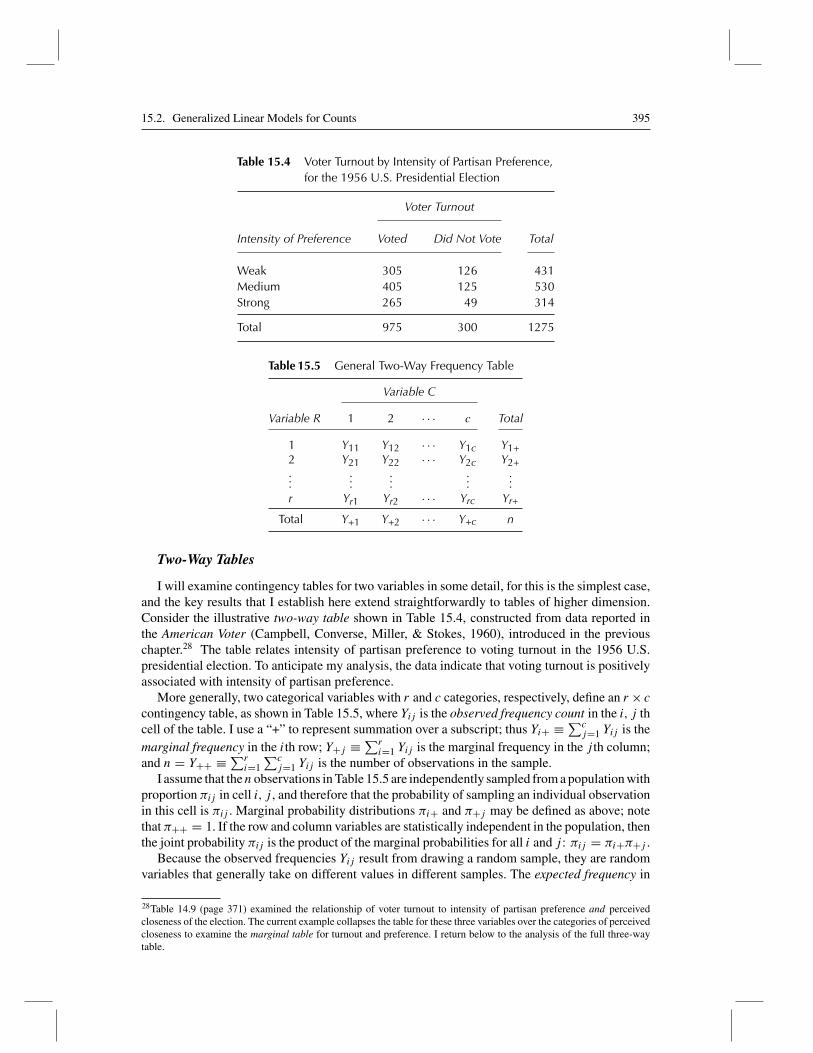
I will examine contingency tables for two variables in some detail, for this is the simplest case,and the key results that I establish here extend straightforwardly to tables of higher dimension.Consider the illustrative two-way table shown in Table 15.4, constructed from data reported inthe American Voter (Campbell, Converse, Miller, & Stokes, 1960), introduced in the previouschapter.28 The table relates intensity of partisan preference to voting turnout in the 1956 U.S.presidential election. To anticipate my analysis, the data indicate that voting turnout is positivelyassociated with intensity of partisan preference.
More generally, two categorical variables with r and c categories, respectively, define an r × ccontingency table, as shown in Table 15.5, where Yij is the observed frequency count in the i, j thcell of the table. I use a “+” to represent summation over a subscript; thus Yi+ ≡ ∑c
j=1 Yij is themarginal frequency in the ith row; Y+j ≡ ∑r
i=1 Yij is the marginal frequency in the j th column;and n = Y++ ≡ ∑r
i=1∑cj=1 Yij is the number of observations in the sample.
I assume that thenobservations in Table 15.5 are independently sampled from a population withproportion πij in cell i, j , and therefore that the probability of sampling an individual observationin this cell is πij . Marginal probability distributions πi+ and π+j may be defined as above; notethat π++ = 1. If the row and column variables are statistically independent in the population, thenthe joint probability πij is the product of the marginal probabilities for all i and j : πij = πi+π+j .
Because the observed frequencies Yij result from drawing a random sample, they are randomvariables that generally take on different values in different samples. The expected frequency in
28Table 14.9 (page 371) examined the relationship of voter turnout to intensity of partisan preference and perceivedcloseness of the election. The current example collapses the table for these three variables over the categories of perceivedcloseness to examine the marginal table for turnout and preference. I return below to the analysis of the full three-waytable.
396 Chapter 15. Generalized Linear Models
cell i, j is μij ≡ E(Yij ) = nπij . If the variables are independent, then we have μij = nπi+π+j .Moreover, because μi+ = ∑c
j=1 nπij = nπi+ and μ+j = ∑ri=1 nπij = nπ+j , we may write
μij = μi+μ+j /n. Taking the log of both sides of this last equation produces
ηij ≡ loge μij = loge μi+ + loge μ+j − loge n (15.8)
That is, under independence, the log expected frequencies ηij depend additively on the logs of therow marginal expected frequencies, the column marginal expected frequencies, and the samplesize. As Fienberg (1980, pp. 13–14) points out, Equation 15.8 is reminiscent of a main-effectstwo-way ANOVA model, where − loge n plays the role of the constant, loge μi+ and loge μ+j areanalogous to “main-effect” parameters, and ηij appears in place of the response-variable mean.If we impose ANOVA-like sigma constraints on the model, we may reparametrize Equation 15.8as follows:
ηij = μ+ αi + βj (15.9)
where α+ ≡ ∑αi = 0 and β+ ≡ ∑
βj = 0. Equation 15.9 is the loglinear model for indepen-dence in the two-way table. Solving for the parameters of the model, we obtain
μ = η++rc
(15.10)
αi = ηi+c
− μ
βj = η+jr
− μ
It is important to stress that although the loglinear model is formally similar to an ANOVAmodel, the meaning of the two models differs importantly: In analysis of variance, the αi andβj are main-effect parameters, specifying the partial relationship of the (quantitative) responsevariable to each explanatory variable. The loglinear model in Equation 15.9, in contrast, does notdistinguish a response variable, and, because it is a model for independence, specifies that the rowand column variables in the contingency table are unrelated; for this model, the αi and βj merelyexpress the relationship of the log expected cell frequencies to the row and column marginals.The model for independence describes rc expected frequencies in terms of
1 + (r − 1)+ (c − 1) = r + c − 1
independent parameters.By analogy to the two-way ANOVA model, we can add parameters to extend the loglinear
model to data for which the row and column classifications are not independent in the populationbut rather are related in an arbitrary manner:
ηij = μ+ αi + βj + γij (15.11)
where α+ = β+ = γi+ = γ+j = 0 for all i and j . As before, we may write the parameters of themodel in terms of the log expected counts ηij . Indeed, the solution for μ, αi , and βj are the sameas in Equation 15.10, and
γij = ηij − μ− αi − βj
By analogy to the ANOVA model, the γij in the loglinear model are often called “interactions,”but this usage is potentially confusing. I will therefore instead refer to the γij as associationparameters because they represent deviations from independence.
15.2. Generalized Linear Models for Counts 397
Under the model in Equation 15.11, called the saturated model for the two-way table, thenumber of independent parameters is equal to the number of cells in the table,
1 + (r − 1)+ (c − 1)+ (r − 1)(c − 1) = rc
The model is therefore capable of capturing any pattern of association in a two-way table.Remarkably, maximum-likelihood estimates for the parameters of a loglinear model (that is,
in the present case, either the model for independence in Equation 15.9 or the saturated model inEquation 15.11) may be obtained by treating the observed cell counts Yij as the response variablein a Poisson GLM; the log expected counts ηij are then just the linear predictor for the GLM, asthe notation suggests.29
The constraint that all γij = 0 imposed by the model of independence can be tested by alikelihood-ratio test, contrasting the model of independence (Equation 15.9) with the more gen-eral model (Equation 15.11). Because the latter is a saturated model, its residual deviance isnecessarily 0, and the likelihood-ratio statistic for the hypothesis of independence H0: γij = 0is simply the residual deviance for the independence model, which has (r − 1)(c − 1) residualdegrees of freedom. Applied to the illustrative two-way table for the American Voter data, we getG2
0 = 19.428 with (3 − 1)(2 − 1) = 2 degrees of freedom, for which p < .0001, suggesting thatthere is strong evidence that intensity of preference and turnout are related.30
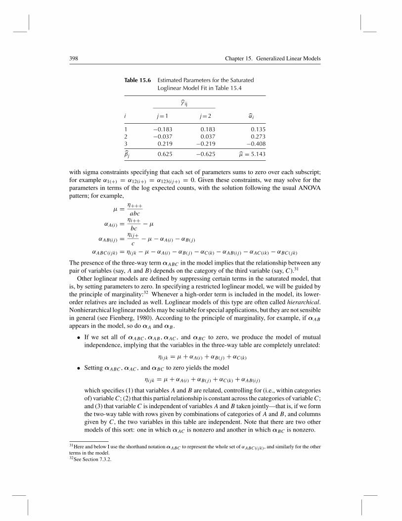
Maximum-likelihood estimates of the parameters of the saturated loglinear model are shown inTable 15.6. It is clear from the estimated association parameters γij that turning out to vote, j = 1,increases with partisan preference (and, of course, that not turning out to vote, j = 2, decreaseswith preference).
Three-Way Tables
The saturated loglinear model for a three-way (a × b × c) table for variables A, B, and C isdefined in analogy to the three-way ANOVA model, although, as in the case of two-way tables,the meaning of the parameters is different:
ηijk = μ+ αA(i) + αB(j) + αC(k) + αAB(ij) + αAC(ik) + αBC(jk) + αABC(ijk) (15.12)
29* The reason that this result is remarkable is that a direct route to a likelihood function for the loglinear model leads tothe multinomial distribution (discussed in Appendix D on probability and estimation), not to the Poisson distribution. Thatis, selecting n independent observations from a population characterized by cell probabilities πij results in cell countsfollowing the multinomial distribution,
p(y11, . . . , yrc) = n!r∏i=1
c∏j=1
yij !
r∏i=1
c∏j=1
πnijij
= n!r∏i=1
c∏j=1
yij !
r∏i=1
c∏j=1
(μijn
)nij
Noting that the expected counts μij are functions of the parameters of the loglinear model leads to the multinomiallikelihood function for the model. It turns out that maximizing this multinomial likelihood is equivalent to maximizingthe likelihood for the Poisson GLM described in the text (see, e.g., Fienberg, 1980, app. II).30This test is very similar to the usual Pearson chi-square test for independence in a two-way table. See Exercise 15.3for details, and for an alternative formula for calculating the likelihood-ratio test statistic G2
0 directly from the observedfrequencies, Yij , and estimated expected frequencies under independence, μij .
398 Chapter 15. Generalized Linear Models
Table 15.6 Estimated Parameters for the SaturatedLoglinear Model Fit in Table 15.4
γ ij
i j = 1 j = 2 αi
1 −0.183 0.183 0.1352 −0.037 0.037 0.2733 0.219 −0.219 −0.408
β j 0.625 −0.625 μ = 5.143
with sigma constraints specifying that each set of parameters sums to zero over each subscript;for example α1(+) = α12(i+) = α123(ij+) = 0. Given these constraints, we may solve for theparameters in terms of the log expected counts, with the solution following the usual ANOVApattern; for example,
μ = η+++abc
αA(i) = ηi++bc
− μ
αAB(ij) = ηij+c
− μ− αA(i) − αB(j)
αABC(ijk) = ηijk − μ− αA(i) − αB(j) − αC(k) − αAB(ij) − αAC(ik) − αBC(jk)
The presence of the three-way termαABC in the model implies that the relationship between anypair of variables (say, A and B) depends on the category of the third variable (say, C).31
Other loglinear models are defined by suppressing certain terms in the saturated model, thatis, by setting parameters to zero. In specifying a restricted loglinear model, we will be guided bythe principle of marginality:32 Whenever a high-order term is included in the model, its lower-order relatives are included as well. Loglinear models of this type are often called hierarchical.Nonhierarchical loglinear models may be suitable for special applications, but they are not sensiblein general (see Fienberg, 1980). According to the principle of marginality, for example, if αABappears in the model, so do αA and αB .
• If we set all of αABC,αAB,αAC, and αBC to zero, we produce the model of mutualindependence, implying that the variables in the three-way table are completely unrelated:
ηijk = μ+ αA(i) + αB(j) + αC(k)
• Setting αABC,αAC, and αBC to zero yields the model
ηijk = μ+ αA(i) + αB(j) + αC(k) + αAB(ij)
which specifies (1) that variablesA and B are related, controlling for (i.e., within categoriesof) variableC; (2) that this partial relationship is constant across the categories of variableC;and (3) that variableC is independent of variablesA andB taken jointly—that is, if we formthe two-way table with rows given by combinations of categories of A and B, and columnsgiven by C, the two variables in this table are independent. Note that there are two othermodels of this sort: one in which αAC is nonzero and another in which αBC is nonzero.
31Here and below I use the shorthand notation αABC to represent the whole set of αABC(ijk), and similarly for the otherterms in the model.32See Section 7.3.2.
15.2. Generalized Linear Models for Counts 399
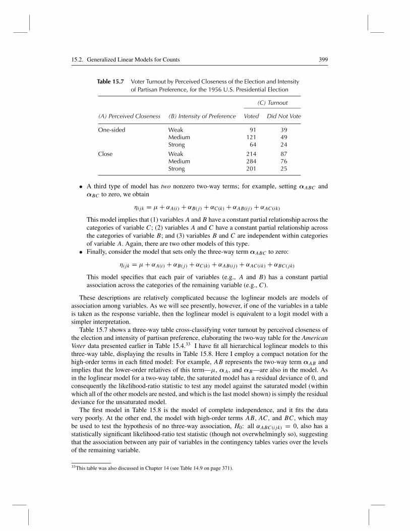
Table 15.7 Voter Turnout by Perceived Closeness of the Election and Intensityof Partisan Preference, for the 1956 U.S. Presidential Election
(C) Turnout
(A) Perceived Closeness (B) Intensity of Preference Voted Did Not Vote
One-sided Weak 91 39Medium 121 49Strong 64 24
Close Weak 214 87Medium 284 76Strong 201 25
• A third type of model has two nonzero two-way terms; for example, setting αABC andαBC to zero, we obtain
ηijk = μ+ αA(i) + αB(j) + αC(k) + αAB(ij) + αAC(ik)
This model implies that (1) variablesA and B have a constant partial relationship across thecategories of variable C; (2) variables A and C have a constant partial relationship acrossthe categories of variable B; and (3) variables B and C are independent within categoriesof variable A. Again, there are two other models of this type.
• Finally, consider the model that sets only the three-way term αABC to zero:
ηijk = μ+ αA(i) + αB(j) + αC(k) + αAB(ij) + αAC(ik) + αBC(jk)
This model specifies that each pair of variables (e.g., A and B) has a constant partialassociation across the categories of the remaining variable (e.g., C).
These descriptions are relatively complicated because the loglinear models are models ofassociation among variables. As we will see presently, however, if one of the variables in a tableis taken as the response variable, then the loglinear model is equivalent to a logit model with asimpler interpretation.
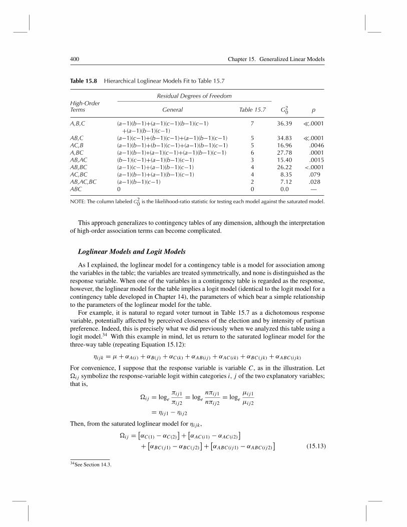
Table 15.7 shows a three-way table cross-classifying voter turnout by perceived closeness ofthe election and intensity of partisan preference, elaborating the two-way table for the AmericanVoter data presented earlier in Table 15.4.33 I have fit all hierarchical loglinear models to thisthree-way table, displaying the results in Table 15.8. Here I employ a compact notation for thehigh-order terms in each fitted model: For example, AB represents the two-way term αAB andimplies that the lower-order relatives of this term—μ, αA, and αB—are also in the model. Asin the loglinear model for a two-way table, the saturated model has a residual deviance of 0, andconsequently the likelihood-ratio statistic to test any model against the saturated model (withinwhich all of the other models are nested, and which is the last model shown) is simply the residualdeviance for the unsaturated model.
The first model in Table 15.8 is the model of complete independence, and it fits the datavery poorly. At the other end, the model with high-order terms AB,AC, and BC, which maybe used to test the hypothesis of no three-way association, H0: all αABC(ijk) = 0, also has astatistically significant likelihood-ratio test statistic (though not overwhelmingly so), suggestingthat the association between any pair of variables in the contingency tables varies over the levelsof the remaining variable.
33This table was also discussed in Chapter 14 (see Table 14.9 on page 371).
400 Chapter 15. Generalized Linear Models
Table 15.8 Hierarchical Loglinear Models Fit to Table 15.7
Residual Degrees of FreedomHigh-OrderTerms General Table 15.7 G2
0 p
A,B,C (a−1)(b−1)+(a−1)(c−1)(b−1)(c−1) 7 36.39 �.0001+(a−1)(b−1)(c−1)
AB,C (a−1)(c−1)+(b−1)(c−1)+(a−1)(b−1)(c−1) 5 34.83 �.0001AC,B (a−1)(b−1)+(b−1)(c−1)+(a−1)(b−1)(c−1) 5 16.96 .0046A,BC (a−1)(b−1)+(a−1)(c−1)+(a−1)(b−1)(c−1) 6 27.78 .0001AB,AC (b−1)(c−1)+(a−1)(b−1)(c−1) 3 15.40 .0015AB,BC (a−1)(c−1)+(a−1)(b−1)(c−1) 4 26.22 <.0001AC,BC (a−1)(b−1)+(a−1)(b−1)(c−1) 4 8.35 .079AB,AC,BC (a−1)(b−1)(c−1) 2 7.12 .028ABC 0 0 0.0 —
NOTE: The column labeled G20 is the likelihood-ratio statistic for testing each model against the saturated model.
This approach generalizes to contingency tables of any dimension, although the interpretationof high-order association terms can become complicated.
Loglinear Models and Logit Models
As I explained, the loglinear model for a contingency table is a model for association amongthe variables in the table; the variables are treated symmetrically, and none is distinguished as theresponse variable. When one of the variables in a contingency table is regarded as the response,however, the loglinear model for the table implies a logit model (identical to the logit model for acontingency table developed in Chapter 14), the parameters of which bear a simple relationshipto the parameters of the loglinear model for the table.
For example, it is natural to regard voter turnout in Table 15.7 as a dichotomous responsevariable, potentially affected by perceived closeness of the election and by intensity of partisanpreference. Indeed, this is precisely what we did previously when we analyzed this table using alogit model.34 With this example in mind, let us return to the saturated loglinear model for thethree-way table (repeating Equation 15.12):
ηijk = μ+ αA(i) + αB(j) + αC(k) + αAB(ij) + αAC(ik) + αBC(jk) + αABC(ijk)
For convenience, I suppose that the response variable is variable C, as in the illustration. Let�ij symbolize the response-variable logit within categories i, j of the two explanatory variables;that is,
�ij = logeπij1
πij2= loge
nπij1
nπij2= loge
μij1
μij2
= ηij1 − ηij2
Then, from the saturated loglinear model for ηijk ,
�ij = [αC(1) − αC(2)
]+ [αAC(i1) − αAC(i2)
]+ [αBC(j1) − αBC(j2)
]+ [αABC(ij1) − αABC(ij2)
](15.13)
34See Section 14.3.

15.2. Generalized Linear Models for Counts 401
Noting that the first bracketed term in Equation 15.13 does not depend on the explanatory variables,that the second depends only upon variable A, and so forth, let us rewrite this equation in thefollowing manner:
�ij = ω + ωA(i) + ωB(j) + ωAB(ij) (15.14)
where, because of the sigma constraints on the αs,
ω ≡ αC(1) − αC(2) = 2αC(1)ωA(i) ≡ αAC(i1) − αAC(i2) = 2αAC(i1)ωB(j) ≡ αBC(j1) − αBC(j2) = 2αBC(j1)
ωAB(ij) ≡ αABC(ij1) − αABC(ij2) = 2αABC(ij1)
Furthermore, because they are defined as twice the αs, the ωs are also constrained to sum to zeroover any subscript:
ωA(+) = ωB(+) = ωAB(i+) = ωAB(+j) = 0, for all i and j
Note that the loglinear-model parameters for the association of the explanatory variablesA andB do not appear in Equation 15.13. This equation (or, equivalently, Equation 15.14), the saturatedlogit model for the table, therefore shows how the response-variable log-odds depend on theexplanatory variables and their interactions. In light of the constraints that they satisfy, the ωsare interpretable as ANOVA-like effect parameters, and indeed we have returned to the binomiallogit model for a contingency table introduced in the previous chapter: Note, for example, thatthe likelihood-ratio test for the three-way term in the loglinear model for the American Voterdata (given in the penultimate line of Table 15.8) is identical to the likelihood-ratio test for theinteraction between closeness and preference in the logit model fit to these data (see Table 14.11on page 373).
A similar argument may also be pursued with respect to any unsaturated loglinear model forthe three-way table: Each such model implies a model for the response-variable logits. Because,however, our purpose is to examine the effects of the explanatory variables on the response, andnot to explore the association between the explanatory variables, we generally include αAB andits lower-order relatives in any model that we fit, thereby treating the association (if any) betweenvariables A and B as given. Furthermore, a similar argument to the one developed here can beapplied to a table of any dimension that has a response variable, and to a response variable withmore than two categories. In the latter event, the loglinear model is equivalent to a multinomiallogit model for the table, and in any event, we would generally include in the loglinear model aterm of dimension one less than the table corresponding to all associations among the explanatoryvariables.
Loglinear models for contingency tables bear a formal resemblance to analysis-of-variancemodels and can be fit to data as Poisson generalized linear models with a log link.The loglinear model for a contingency table, however, treats the variables in the tablesymmetrically—none of the variables is distinguished as a response variable—and con-sequently the parameters of the model represent the associations among the variables,not the effects of explanatory variables on a response. When one of the variables is con-strued as the response, the loglinear model reduces to a binomial or multinomial logitmodel.
402 Chapter 15. Generalized Linear Models
15.3 Statistical Theory forGeneralized Linear Models*
In this section, I revisit with greater rigor and more detail many of the points raised in the precedingsections.35
15.3.1 Exponential Families
As much else in modern statistics, the insight that many of the most important distributionsin statistics could be expressed in the following common “linear-exponential” form was due toR. A. Fisher:
p(y; θ, φ) = exp
[yθ − b(θ)
a(φ)+ c(y, φ)
](15.15)
where
• p(y; θ, φ) is the probability function for the discrete random variable Y , or the probability-density function for continuous Y .
• a(·), b(·), and c(·) are known functions that vary from one exponential family to another(see below for examples).
• θ = gc(μ), the canonical parameter for the exponential family in question, is a functionof the expectation μ ≡ E(Y ) of Y ; moreover, the canonical link function gc(·) does notdepend on φ.
• φ > 0 is a dispersion parameter, which, in some families, takes on a fixed, known value,while in other families it is an unknown parameter to be estimated from the data along with θ .
Consider, for example, the normal or Gaussian distribution with mean μ and variance σ 2, thedensity function for which is given in Equation 15.1 (on page 382). To put the normal distribution inthe form of Equation 15.15 requires some heroic algebraic manipulation, eventually producing36
p(y; θ, φ) = exp
{yθ − θ2/2
φ− 1
2
[y2
φ+ loge(2πφ)
]}
with θ = gc(μ) = μ; φ = σ 2 ; a(φ) = φ; b(θ) = θ2/2; and c(y, φ) = − 12
[y2/φ + loge(2πφ)
].
Now consider the binomial distribution in Equation 15.2 (page 382), where Y is the proportionof “successes” in n independent binary trials, and μ is the probability of success on an individualtrial. Written after more algebraic gymnastics as an exponential family,37
p(y; θ, φ) = exp
[yθ − loge(1 + eθ )
1/n+ loge
(n
ny
)]
with θ = gc(μ) = loge[μ/(1 − μ)]; φ = 1; a(φ) = 1/n; b(θ) = loge(1 + eθ ); and c(y, φ) =loge
(nny
).
Similarly, the Poisson, gamma, and inverse-Gaussian families can all be put into the form ofEquation 15.15, using the results given in Table 15.9.38
35The exposition here owes a debt to Chapter 2 of McCullagh and Nelder (1989), which has become the standard sourceon GLMs, and to the remarkly lucid and insightful briefer treatment of the topic by Firth (1991).36See Exercise 15.4.37See Exercise 15.5.38See Exercise 15.6.
15.3. Statistical Theory for Generalized Linear Models* 403
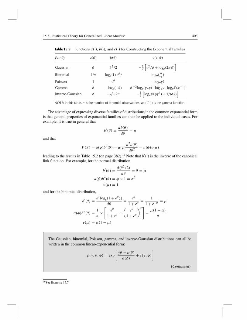
Table 15.9 Functions a(·), b(·), and c(·) for Constructing the Exponential Families
Family a(φ) b(θ) c(y, φ)
Gaussian φ θ2/2 −12
[y2/φ + loge(2πφ)
]Binomial 1/n loge(1+eθ ) loge
( nny)
Poisson 1 eθ −logey!
Gamma φ −loge(−θ) φ−2loge(y/φ)−log ey−loge�(φ−1)
Inverse-Gaussian φ −√−2θ −12
[loge(πφy3)+ 1/(φy)
]NOTE: In this table, n is the number of binomial observations, and �(·) is the gamma function.
The advantage of expressing diverse families of distributions in the common exponential formis that general properties of exponential families can then be applied to the individual cases. Forexample, it is true in general that
b′(θ) ≡ db(θ)
dθ= μ
and that
V (Y ) = a(φ)b′′(θ) = a(φ)d2b(θ)
dθ2= a(φ)v(μ)
leading to the results in Table 15.2 (on page 382).39 Note that b′(·) is the inverse of the canonicallink function. For example, for the normal distribution,
b′(θ) = d(θ2/2)
dθ= θ = μ
a(φ)b′′(θ) = φ × 1 = σ 2
v(μ) = 1
and for the binomial distribution,
b′(θ) = d[loge(1 + eθ )]
dθ= eθ
1 + eθ= 1
1 + e−θ= μ
a(φ)b′′(θ) = 1
n×[
eθ
1 + eθ−(
eθ
1 + eθ
)2]
= μ(1 − μ)
n
v(μ) = μ(1 − μ)
The Gaussian, binomial, Poisson, gamma, and inverse-Gaussian distributions can all bewritten in the common linear-exponential form:
p(y; θ, φ) = exp
[yθ − b(θ)
a(φ)+ c(y, φ)
]
(Continued)
39See Exercise 15.7.
404 Chapter 15. Generalized Linear Models
(Continued)
where a(·), b(·), and c(·) are known functions that vary from one exponential family toanother; θ = gc(μ) is the canonical parameter for the exponential family in question; gc(·)is the canonical link function; and φ > 0 is a dispersion parameter, which takes on a fixed,known value in some families. It is generally the case that μ = E(Y ) = b′(θ) and thatV (Y ) = a(φ)b′′(θ).
15.3.2 Maximum-LikelihoodEstimation of Generalized Linear Models
The log likelihood for an individual observation Yi follows directly from Equation 15.15(page 402):
loge L(θi, φ;Yi) = yiθi − b(θi)
ai(φ)+ c(Yi, φ)
For n independent observations, we have
loge L(θ, φ; y) =n∑i=1
Yiθi − b(θi)
ai(φ)+ c(Yi, φ) (15.16)
where θ ≡ {θi} and y ≡ {Yi}.Suppose that a GLM uses the link function g(·), so that40
g(μi) = ηi = β0 + β1Xi1 + β2Xi2 + · · · + βkXik
The model therefore expresses the expected values of then observations in terms of a much smallernumber of regression parameters. To get estimating equations for the regression parameters, wehave to differentiate the log likelihood with respect to each coefficient in turn. Let li represent theith component of the log likelihood. Then, by the chain rule,
∂li
∂βj= ∂li
∂θi× dθi
dμi× dμi
dηi× ∂ηi
∂βjfor j = 0, 1, . . . , k (15.17)
After some work, we can rewrite Equation 15.17 as41
∂li
∂βj= yi − μi
ai(φ)v(μi)× dμi
dηi× xij
Summing over observations, and setting the sum to zero, produces the maximum-likelihoodestimating equations for the GLM,
n∑i=1
Yi − μi
aiv(μi)× dμi
dηi× xij = 0, for j = 0, 1, . . . , k (15.18)
where ai ≡ ai(φ)/φ does not depend upon the dispersion parameter, which is constant acrossobservations. For example, in a Gaussian GLM, ai = 1, while in a binomial GLM, ai = 1/ni .
40It is notationally convenient here to write β0 for the regression constant α.41See Exercise 15.8.
15.3. Statistical Theory for Generalized Linear Models* 405
Further simplification can be achieved when g(·) is the canonical link. In this case, themaximum-likelihood estimating equations become
n∑i=1
Yixij
ai=
n∑i=1
μixij
ai
setting the “observed sum” on the left of the equation to the “expected sum” on the right. We notedthis pattern in the estimating equations for logistic-regression models in the previous chapter.42
Nevertheless, even here the estimating equations are (except in the case of the Gaussian familypaired with the identify link) nonlinear functions of the regression parameters and generallyrequire iterative methods for their solution.
Iterative Weighted Least Squares
Let
Zi ≡ ηi + (Yi − μi)dηi
dμi
= ηi + (Yi − μi)g′(μi)
Then
E(Zi) = ηi = β0 + β1Xi1 + β2Xi2 + · · · + βkXik
and
V (Zi) = [g′(μi)
]2aiv(μi)
If, therefore, we could compute theZi , we would be able to fit the model by weighted least-squaresregression of Z on theXs, using the inverses of the V (Zi) as weights.43 Of course, this is not thecase because we do not know the values of theμi and ηi , which, indeed, depend on the regressioncoefficients that we wish to estimate—that is, the argument is essentially circular. This observationsuggested to Nelder and Wedderburn (1972) the possibility of estimating GLMs by iterativeweighted least-squares (IWLS), cleverly turning the circularity into an iterative procedure:
1. Start with initial estimates of the μi and the ηi = g(μi), denoted μ(0)i and η(0)i . A simple
choice is to set μ(0)i = Yi .44
2. At each iteration l, compute the working response variable Z using the values of μ and ηfrom the preceding iteration,
Z(l−1)i = η
(l−1)i +
(Yi − μ
(l−1)i
)g′ (μ(l−1)
i
)
42See Sections 14.1.5 and 14.2.1.43See Section 12.2.2 for a general discussion of weighted least squares.44In certain settings, starting with μ(0)
i= Yi can cause computational difficulties. For example, in a binomial GLM, some
of the observed proportions may be 0 or 1—indeed, for binary data, this will be true for all the observations—requiringus to divide by 0 or to take the log of 0. The solution is to adjust the starting values, which are in any event not critical, to
protect against this possibility. For a binomial GLM, where Yi = 0, we can take μ(0)i
= 0.5/ni , and where Yi = 1, we
can take μ(0)i
= (ni − 0.5)/ni . For binary data, then, all the μ(0)i
are 0.5.
406 Chapter 15. Generalized Linear Models
along with weights
W(l−1)i = 1[
g′(μ(l−1)i
)]2aiv
(μ(l−1)i
)3. Fit a weighted least-squares regression of Z(l−1) on the Xs, using the W(l−1) as weights.
That is, compute
b(l) =(
X′W(l−1)X)−1
X′W(l−1)z(l−1)
where b(l)(k+1×1)
is the vector of regression coefficients at the current iteration; X(n×k+1)
is
(as usual) the model matrix; W(l−1)
(n×n)≡ diag
{W(l−1)i
}is the diagonal weight matrix; and
z(l−1)
(n×1)≡{Z(l−1)i
}is the working-response vector.
4. Repeat Steps 2 and 3 until the regression coefficients stabilize, at which point b convergesto the maximum-likelihood estimates of the βs.
Applied to the canonical link, IWLS is equivalent to the Newton-Raphson method (as wediscovered for a logit model in the previous chapter); more generally, IWLS implements Fisher’s“method of scoring.”
Estimating the Dispersion Parameter
Note that we do not require an estimate of the dispersion parameter to estimate the regressioncoefficients in a GLM. Although it is in principle possible to estimate φ by maximum likelihoodas well, this is rarely done. Instead, recall that V (Yi) = φaiv(μi). Solving for the dispersionparameter, we get φ = V (Yi)/aiv(μi), suggesting the method of moments estimator
φ = 1
n− k − 1
∑ (Yi − μi)2
aiv(μi)(15.19)
The estimated asymptotic covariance matrix of the coefficients is then obtained from the lastIWLS iteration as
V(b) = φ(X′WX
)−1
Because the maximum-likelihood estimator b is asymptotically normally distributed, V(b) maybe used as the basis for Wald tests of the regression parameters.
The maximum-likelihood estimating equations for generalized linear models take the com-mon form
n∑i=1
Yi − μi
aiv(μi)× dμi
dηi× xij = 0, for j = 0, 1, . . . , k
15.3. Statistical Theory for Generalized Linear Models* 407
These equations are generally nonlinear and therefore have no general closed-form solu-tion, but they can be solved by iterated weighted least squares (IWLS). The estimatingequations for the coefficients do not involve the dispersion parameter, which (for modelsin which the dispersion is not fixed) then can be estimated as
φ = 1
n− k − 1
∑ (Yi − μi)2
aiv(μi)
The estimated asymptotic covariance matrix of the coefficients is
V(b) = φ(X′WX
)−1
where b is the vector of estimated coefficients and W is a diagonal matrix of weights fromthe last IWLS iteration.
Quasi-Likelihood Estimation
The argument leading to IWLS estimation rests only on the linearity of the relationshipbetween η = g(μ) and the Xs, and on the assumption that V (Y ) depends in a particularmanner on a dispersion parameter and μ. As long as we can express the transformed meanof Y as a linear function of the Xs, and can write down a variance function for Y (expressingthe conditional variance of Y as a function of its mean and a dispersion parameter), we canapply the “maximum-likelihood” estimating equations (Equation 15.18 on page 404) and obtainestimates by IWLS—even without committing ourselves to a particular conditional distributionfor Y .
This is the method of quasi-likelihood estimation, introduced by Wedderburn (1974), and ithas been shown to retain many of the properties of maximum-likelihood estimation: Althoughthe quasi-likelihood estimator may not be maximally asymptotically efficient, it is consistentand has the same asymptotic distribution as the maximum-likelihood estimator of a GLM in anexponential family.45 We can think of quasi-likelihood estimation of GLMs as analogous to least-squares estimation of linear regression models with potentially non-normal errors: Recall that aslong as the relationship between Y and the Xs is linear, the error variance is constant, and theobservations are independently sampled, the theory underlying OLS estimation applies—althoughthe OLS estimator may no longer be maximally efficient.46
The maximum-likelihood estimating equations, and IWLS estimation, can be appliedwhenever we can express the transformed mean of Y as a linear function of the Xs, andcan write the conditional variance of Y as a function of its mean and (possibly) a dispersionparameter—even when we do not specify a particular conditional distribution for Y . Theresulting quasi-likelihood estimator shares many of the properties of maximum-likelihoodestimators.
45See, for example, McCullagh and Nelder (1989, chap. 9) and McCullagh (1991).46See Chapter 9.
408 Chapter 15. Generalized Linear Models
15.3.3 Hypothesis Tests
Analysis of Deviance
Originally (in Equation 15.16 on page 404), I wrote the log likelihood for a GLM as a functionloge L(θ, φ; y) of the canonical parameters θ for the observations. Becauseμi = g−1
c (θi), for thecanonical link gc(·), we can equally well think of the log likelihood as a function of the expectedresponse, and therefore can write the maximized log likelihood as loge L(μ, φ; y). If we thendedicate a parameter to each observation, so that μi = Yi (e.g., by removing the constant fromthe regression model and defining a dummy regressor for each observation), the log likelihoodbecomes loge L(y, φ; y). The residual deviance under the initial model is twice the difference inthese log likelihoods:
D(y; μ) ≡ 2[loge L(y, φ; y)− loge L(μ, φ; y)] (15.20)
= 2n∑i=1
[loge L(Yi, φ;Yi)− loge L(μi, φ;Yi)]
= 2n∑i=1
Yi [g(Yi)− g(μi)] − b [g(Yi)] + b [g(μi)]
ai
Dividing the residual deviance by the estimated dispersion parameter produces the scaleddeviance, D∗(y; μ) ≡ D(y; μ)/φ. As explained in Section 15.1.1, deviances are the buildingblocks of likelihood-ratio and F -tests for GLMs.
Applying Equation 15.20 to the Gaussian distribution, where gc(·) is the identity link, ai = 1,and b(θ) = θ2/2, produces (after some simplification)
D(y; μ) =∑
(Yi − μ)2
that is, the residual sum of squares for the model. Similarly, applying Equation 15.20 to thebinomial distribution, where gc(·) is the logit link, ai = ni , and b(θ) = loge(1 + eθ ), we get(after quite a bit of simplification)47
D(y; μ) = 2∑
ni
[Yi loge
Yi
μi+ (1 − Yi) loge
1 − Yi
1 − μi
]
The residual deviance for a model is twice the difference in the log likelihoods for thesaturated model, which dedicates one parameter to each observation, and the model inquestion:
D(y; μ) ≡ 2[loge L(y, φ; y)− loge L(μ, φ; y)]
= 2n∑i=1
Yi [g(Yi)− g(μi)] − b [g(Yi)] + b [g(μi)]
ai
Dividing the residual deviance by the estimated dispersion parameter produces the scaleddeviance, D∗(y; μ) ≡ D(y; μ)/φ.
47See Exercise 15.9, which also develops formulas for the deviance in Poisson, gamma, and inverse-Gaussian models.
15.3. Statistical Theory for Generalized Linear Models* 409
Testing General Linear Hypotheses
As was the case for linear models,48 we can formulate a test for the general linear hypothesis
H0: L(q×k+1)
β(k+1×1)
= c(q×1)
where the hypothesis matrix L and right-hand-side vector c contain pre-specified constants; usu-ally, c = 0. For a GLM, the Wald statistic
Z20 = (Lb − c)′ [LV(b)L′]−1 (Lb − c)
follows an asymptotic chi-square distribution with q degrees of freedom under the hypothesis.The simplest application of this result is to the Wald statistic Z0 = Bj/SE(Bj ), testing that anindividual regression coefficient is zero. Here, Z0 follows a standard-normal distribution underH0: βj = 0 (or, equivalently, Z2
0 follows a chi-square distribution with one degree of freedom).Alternatively, when the dispersion parameter is estimated from the data, we can calculate the
test statistic
F0 = (Lb − c)′ [LV(b)L′]−1 (Lb − c)q
which is distributed as Fq,n−k−1 under H0. Applied to an individual coefficient, t0 = ±√F0 =
Bj/SE(Bj ) produces a t-test on n− k − 1 degrees of freedom.
To test the general linear hypothesis H0: Lβ = c, where the hypothesis matrix L hasq rows, we can compute the Wald chi-square test statistic Z2
0 = (Lb − c)′ [LV(b)L′]−1
(Lb − c), with q degrees of freedom. Alternatively, if the dispersion parameter is esti-mated from the data, we can compute the F -test statistic F0 = (Lb − c)′ [LV(b)L′]−1
(Lb − c) /q on q and n− k − 1 degrees of freedom.
Testing Nonlinear Hypotheses
It is occasionally of interest to test a hypothesis or construct a confidence interval for a nonlinearfunction of the parameters of a linear or generalized linear model. If the nonlinear function inquestion is a differentiable function of the regression coefficients, then an approximate asymptoticstandard error may be obtained by the delta method.49
Suppose that we are interested in the function
γ ≡ f (β) = f (β0, β1, . . . , βk)
where, for notational convenience, I have used β0 to denote the regression constant. Thefunction f (β) need not use all the regression coefficients (see the example below). The
48See Section 9.4.4.49The delta method (Rao, 1973) is described in Appendix D on probability and estimation. The method employs a first-order (i.e., linear) Taylor-series approximation to the nonlinear function. The delta method is appropriate here because themaximum-likelihood (or quasi-likelihood) estimates of the coefficients of a GLM are asymptotically normally distributed.Indeed, the procedure described in this section is applicable whenever the parameters of a regression model are normallydistributed and can therefore be applied in a wide variety of contexts—such as to the nonlinear regression models describedin Chapter 17. In small samples, however, the delta-method approximation to the standard error may not be adequate, andthe bootstrapping procedures described in Chapter 21 will usually provide more reliable results.
410 Chapter 15. Generalized Linear Models
maximum-likelihood estimator of γ is simply γ = f (β) (which, as an MLE, is also asymp-totically normal), and the approximate sampling variance of γ is then
V(γ ) ≈k∑j=0
k∑j ′=0
vjj ′ × ∂γ
∂βj× ∂γ
∂βj ′
where vjj ′ is the j, j ′th element of the estimated asymptotic covariance matrix of the coefficients,V(β).
To illustrate the application of this result, imagine that we are interested in determining the max-imum or minimum value of a quadratic partial regression.50 Focusing on the partial relationshipbetween the response variable and a particular X, we have an equation of the form
E(Y ) = · · · + β1X + β2X2 + · · ·
Differentiating this equation with respect to X, we get
dE(Y )
dX= β1 + 2β2X
Setting the derivative to 0 and solving for X produces the value at which the function reseachesa minimum (if β2 is positive) or a maximum (if β2 is negative),
X = − β1
2β2
which is a nonlinear function of the regression coefficients β1 and β2.
For example, in Section 12.3.1, using data from the Canadian Survey of Labour and IncomeDynamics (the “SLID”), I fit a least-squares regression of log wage rate on a quadratic in age,a dummy regressor for sex, and the square of education, obtaining (repeating, and slightly rear-ranging, Equation 12.7 on page 280):
log2 Wages = 0.5725 + 0.1198 × Age − 0.001230 × Age2
(0.0834) (0.0046) (0.000059)+ 0.3195 × Male + 0.002605 × Education2
(0.0180) (0.000113)R2 = .3892
Imagine that we are interested in the age γ ≡ −β1/(2β2) at which wages are at a maximum,holding sex and education constant. The necessary derivatives are
∂γ
∂B1= − 1
2B2= − 1
2(−0.001230)= 406.5
∂γ
∂B2= B1
2B22
= 0.1198
2(−0.001230)2= 39,593
Our point estimate of γ is
γ = − B1
2B2= − 0.1198
2 × 0.001230= 48.70 years
50See Section 17.1 for a discussion of polynomial regression. The application of the delta method to finding the minimumor maximum of a quadratic curve is suggested by Weisberg (2005, sect. 6.1.2).
15.3. Statistical Theory for Generalized Linear Models* 411
The estimated sampling variance of the age coefficient is V (B1) = 2.115 × 10⁻⁵, and of thecoefficient of age-squared, V (B2) = 3.502 × 10⁻⁹; the estimated sampling covariance for thetwo coefficients is C(B1, B2) = −2.685×10⁻⁷. The approximate estimated variance of γ is then
V(γ ) ≈(
2.115 × 10−5)
× 406.52 − (2.685 × 10−7)× 406.5 × 39, 593
− (2.685 × 10−7)× 406.5 × 39, 593 +
(3.502 × 10⁻⁹
)× 39, 5932
= 0.3419
Consequently, the approximate standard error of γ is SE(γ ) ≈ √0.3419 = 0.5847, and an
approximate 95% confidence interval for the age at which income is highest on average is γ =48.70 ± 1.96(0.5847) = (47.55, 49.85).
The delta method may be used to approximate the standard error of a nonlinear functionof regression coefficients in a GLM. If γ ≡ f (β0, β1, . . . , βk), then
V(γ ) ≈k∑j=0
k∑j ′=0
vjj ′∂γ
∂βj
∂γ
∂βj ′
15.3.4 Effect Displays
Let us write the GLM in matrix form, with linear predictor
η(n×1)
= X(n×k+1)
β(k+1×1)
and link function g(μ) = η, where μ is the expectation of the response vector y. As described inSection 15.3.2, we compute the maximum-likelihood estimate b of β, along with the estimatedasymptotic covariance matrix V(b) of b.
Let the rows of X∗ include regressors corresponding to all combinations of values of explana-tory variables appearing in a high-order term of the model (or, for a continuous explanatoryvariable, values spanning the range of the variable), along with typical values of the remainingregressors. The structure of X∗ with respect to interactions, for example, is the same as that of themodel matrix X. Then the fitted values η∗ = X∗b represent the high-order term in question, anda table or graph of these values—or, alternatively, of the fitted values transformed to the scale ofthe response variable, g−1(η∗)—is an effect display. The standard errors of η∗, available as thesquare-root diagonal entries of X∗V(b)X∗′, may be used to compute pointwise confidence intervalsfor the effects, the end-points of which may then also be transformed to the scale of the response.
For example, for the Poisson regression model fit to Ornstein interlocking-directorate data, theeffect display for assets in Figure 15.6(a) (page 390) is constructed by letting assets range betweenits minimum value of 0.062 and maximum of 147.670 billion dollars, fixing the dummy variablesfor nation of control and sector to their sample means—that is, to the observed proportions of thedata in each of the corresponding categories of nation and sector. As noted previously, this is anespecially simple example, because the model includes no interactions. The model was fit withthe log link, and so the estimated effects, which in general are on the scale of the linear predictor,are on the log-count scale; the right-hand axis of the graph shows the corresponding count scale,which is the scale of the response variable.
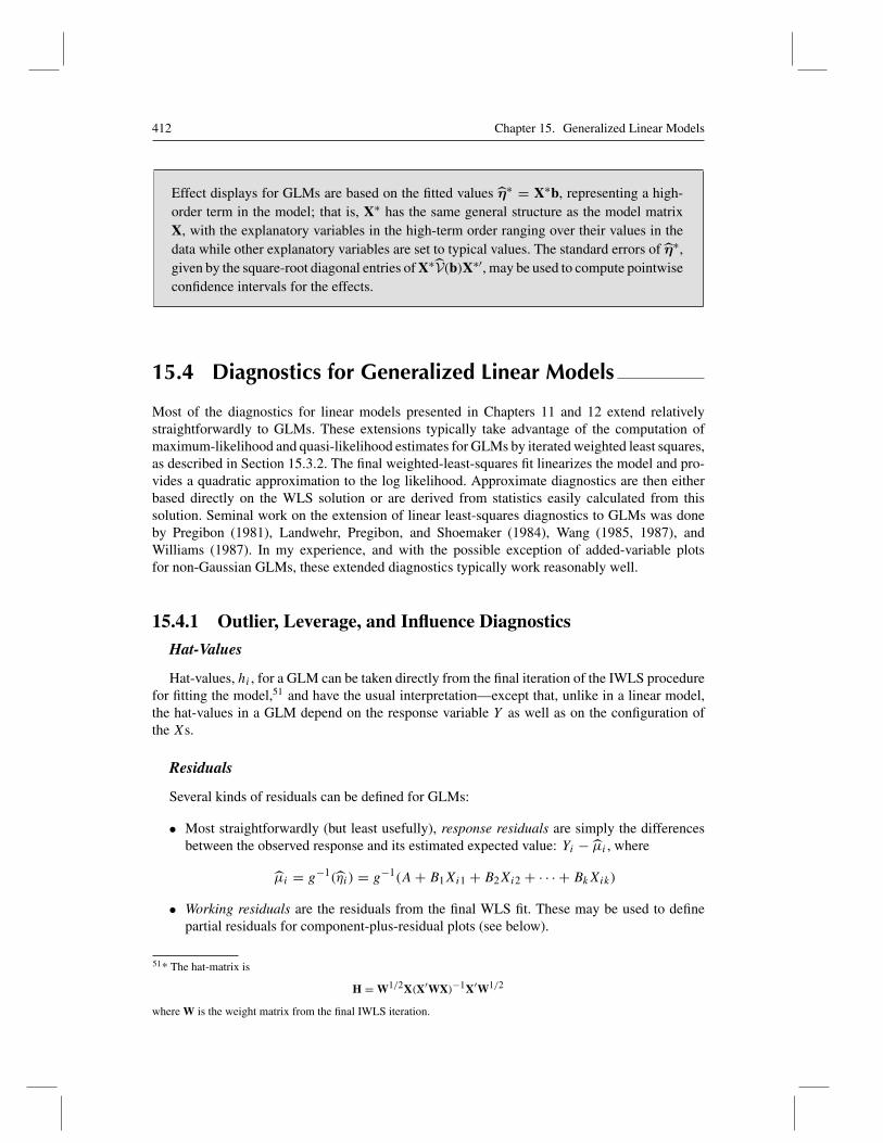
412 Chapter 15. Generalized Linear Models
Effect displays for GLMs are based on the fitted values η∗ = X∗b, representing a high-order term in the model; that is, X∗ has the same general structure as the model matrixX, with the explanatory variables in the high-term order ranging over their values in thedata while other explanatory variables are set to typical values. The standard errors of η∗,given by the square-root diagonal entries of X∗V(b)X∗′, may be used to compute pointwiseconfidence intervals for the effects.
15.4 Diagnostics for Generalized Linear Models
Most of the diagnostics for linear models presented in Chapters 11 and 12 extend relativelystraightforwardly to GLMs. These extensions typically take advantage of the computation ofmaximum-likelihood and quasi-likelihood estimates for GLMs by iterated weighted least squares,as described in Section 15.3.2. The final weighted-least-squares fit linearizes the model and pro-vides a quadratic approximation to the log likelihood. Approximate diagnostics are then eitherbased directly on the WLS solution or are derived from statistics easily calculated from thissolution. Seminal work on the extension of linear least-squares diagnostics to GLMs was doneby Pregibon (1981), Landwehr, Pregibon, and Shoemaker (1984), Wang (1985, 1987), andWilliams (1987). In my experience, and with the possible exception of added-variable plotsfor non-Gaussian GLMs, these extended diagnostics typically work reasonably well.
15.4.1 Outlier, Leverage, and Influence Diagnostics
Hat-Values
Hat-values, hi , for a GLM can be taken directly from the final iteration of the IWLS procedurefor fitting the model,51 and have the usual interpretation—except that, unlike in a linear model,the hat-values in a GLM depend on the response variable Y as well as on the configuration ofthe Xs.
Residuals
Several kinds of residuals can be defined for GLMs:
• Most straightforwardly (but least usefully), response residuals are simply the differencesbetween the observed response and its estimated expected value: Yi − μi , where
μi = g−1(ηi) = g−1(A+ B1Xi1 + B2Xi2 + · · · + BkXik)
• Working residuals are the residuals from the final WLS fit. These may be used to definepartial residuals for component-plus-residual plots (see below).
51* The hat-matrix is
H = W1/2X(X′WX)−1X′W1/2
where W is the weight matrix from the final IWLS iteration.
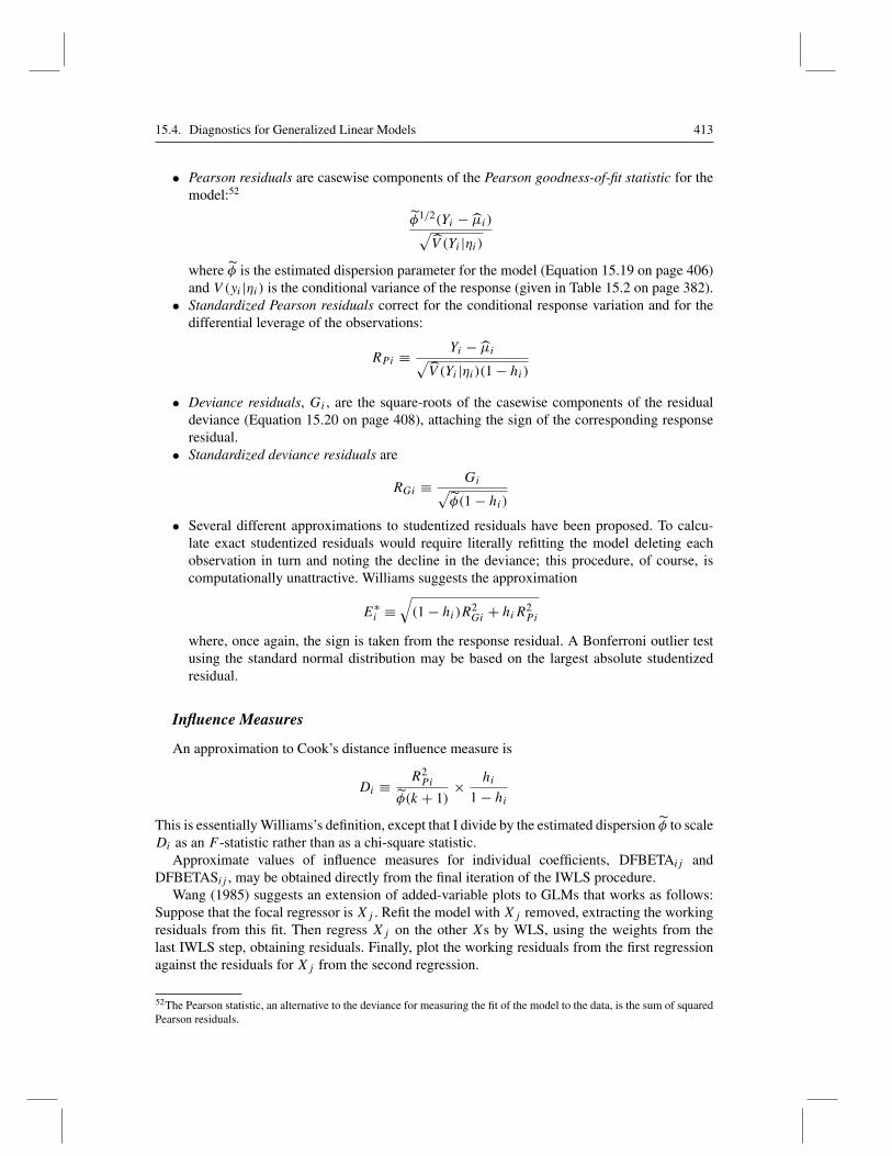
15.4. Diagnostics for Generalized Linear Models 413
• Pearson residuals are casewise components of the Pearson goodness-of-fit statistic for themodel:52
φ1/2(Yi − μi)√V (Yi |ηi)
where φ is the estimated dispersion parameter for the model (Equation 15.19 on page 406)and V (yi |ηi) is the conditional variance of the response (given in Table 15.2 on page 382).
• Standardized Pearson residuals correct for the conditional response variation and for thedifferential leverage of the observations:
RPi ≡ Yi − μi√V (Yi |ηi)(1 − hi)
• Deviance residuals, Gi , are the square-roots of the casewise components of the residualdeviance (Equation 15.20 on page 408), attaching the sign of the corresponding responseresidual.
• Standardized deviance residuals are
RGi ≡ Gi√φ(1 − hi)
• Several different approximations to studentized residuals have been proposed. To calcu-late exact studentized residuals would require literally refitting the model deleting eachobservation in turn and noting the decline in the deviance; this procedure, of course, iscomputationally unattractive. Williams suggests the approximation
E∗i ≡
√(1 − hi)R
2Gi + hiR
2P i
where, once again, the sign is taken from the response residual. A Bonferroni outlier testusing the standard normal distribution may be based on the largest absolute studentizedresidual.
Influence Measures
An approximation to Cook’s distance influence measure is
Di ≡ R2P i
φ(k + 1)× hi
1 − hi
This is essentially Williams’s definition, except that I divide by the estimated dispersion φ to scaleDi as an F -statistic rather than as a chi-square statistic.
Approximate values of influence measures for individual coefficients, DFBETAij andDFBETASij , may be obtained directly from the final iteration of the IWLS procedure.
Wang (1985) suggests an extension of added-variable plots to GLMs that works as follows:Suppose that the focal regressor is Xj . Refit the model with Xj removed, extracting the workingresiduals from this fit. Then regress Xj on the other Xs by WLS, using the weights from thelast IWLS step, obtaining residuals. Finally, plot the working residuals from the first regressionagainst the residuals for Xj from the second regression.
52The Pearson statistic, an alternative to the deviance for measuring the fit of the model to the data, is the sum of squaredPearson residuals.
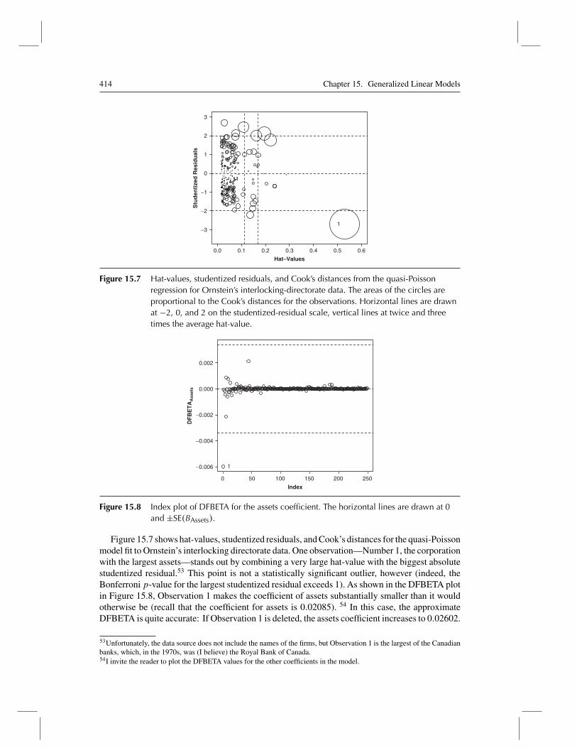
414 Chapter 15. Generalized Linear Models
0.0 0.1 0.2 0.3 0.4 0.5 0.6
Hat–Values
Stu
den
tize
d R
esid
ual
s
1
3
2
1
0
−1
−2
−3
Figure 15.7 Hat-values, studentized residuals, and Cook’s distances from the quasi-Poissonregression for Ornstein’s interlocking-directorate data. The areas of the circles areproportional to the Cook’s distances for the observations. Horizontal lines are drawnat −2, 0, and 2 on the studentized-residual scale, vertical lines at twice and threetimes the average hat-value.
0 50 100 150 200 250
Index
1
DF
BE
TA
Ass
ets
0.002
0.000
−0.002
−0.004
−0.006
Figure 15.8 Index plot of DFBETA for the assets coefficient. The horizontal lines are drawn at 0and ±SE(BAssets).
Figure 15.7 shows hat-values, studentized residuals, and Cook’s distances for the quasi-Poissonmodel fit to Ornstein’s interlocking directorate data. One observation—Number 1, the corporationwith the largest assets—stands out by combining a very large hat-value with the biggest absolutestudentized residual.53 This point is not a statistically significant outlier, however (indeed, theBonferroni p-value for the largest studentized residual exceeds 1). As shown in the DFBETA plotin Figure 15.8, Observation 1 makes the coefficient of assets substantially smaller than it wouldotherwise be (recall that the coefficient for assets is 0.02085). 54 In this case, the approximateDFBETA is quite accurate: If Observation 1 is deleted, the assets coefficient increases to 0.02602.
53Unfortunately, the data source does not include the names of the firms, but Observation 1 is the largest of the Canadianbanks, which, in the 1970s, was (I believe) the Royal Bank of Canada.54I invite the reader to plot the DFBETA values for the other coefficients in the model.
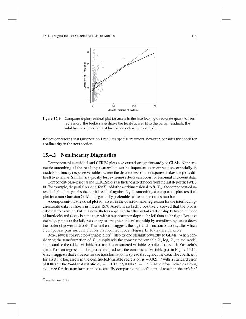
15.4. Diagnostics for Generalized Linear Models 415
0
3
2
1
0
−1
50 100 150
Assets (billions of dollars)
Co
mp
on
ent
+ R
esid
ual
Figure 15.9 Component-plus-residual plot for assets in the interlocking-directorate quasi-Poissonregression. The broken line shows the least-squares fit to the partial residuals; thesolid line is for a nonrobust lowess smooth with a span of 0.9.
Before concluding that Observation 1 requires special treatment, however, consider the check fornonlinearity in the next section.
15.4.2 Nonlinearity Diagnostics
Component-plus-residual and CERES plots also extend straightforwardly to GLMs. Nonpara-metric smoothing of the resulting scatterplots can be important to interpretation, especially inmodels for binary response variables, where the discreteness of the response makes the plots dif-ficult to examine. Similar (if typically less extreme) effects can occur for binomial and count data.
Component-plus-residualandCERESplotsusethelinearizedmodelfromthelaststepoftheIWLSfit.Forexample, thepartial residual forXj adds theworkingresidual toBjXij ; thecomponent-plus-residual plot then graphs the partial residual againstXj . In smoothing a component-plus-residualplot for a non-Gaussian GLM, it is generally preferable to use a nonrobust smoother.
A component-plus-residual plot for assets in the quasi-Poisson regression for the interlocking-directorate data is shown in Figure 15.9. Assets is so highly positively skewed that the plot isdifferent to examine, but it is nevertheless apparent that the partial relationship between numberof interlocks and assets is nonlinear, with a much steeper slope at the left than at the right. Becausethe bulge points to the left, we can try to straighten this relationship by transforming assets downthe ladder of power and roots. Trial and error suggests the log transformation of assets, after whicha component-plus-residual plot for the modified model (Figure 15.10) is unremarkable.
Box-Tidwell constructed-variable plots55 also extend straightforwardly to GLMs: When con-sidering the transformation of Xj , simply add the constructed variable Xj loge Xj to the modeland examine the added-variable plot for the constructed variable. Applied to assets in Ornstein’squasi-Poisson regression, this procedure produces the constructed-variable plot in Figure 15.11,which suggests that evidence for the transformation is spread throughout the data. The coefficientfor assets × logeassets in the constructed-variable regression is −0.02177 with a standard errorof 0.00371; the Wald-test statisticZ0 = −0.02177/0.00371 = −5.874 therefore indicates strongevidence for the transformation of assets. By comparing the coefficient of assets in the original
55See Section 12.5.2.
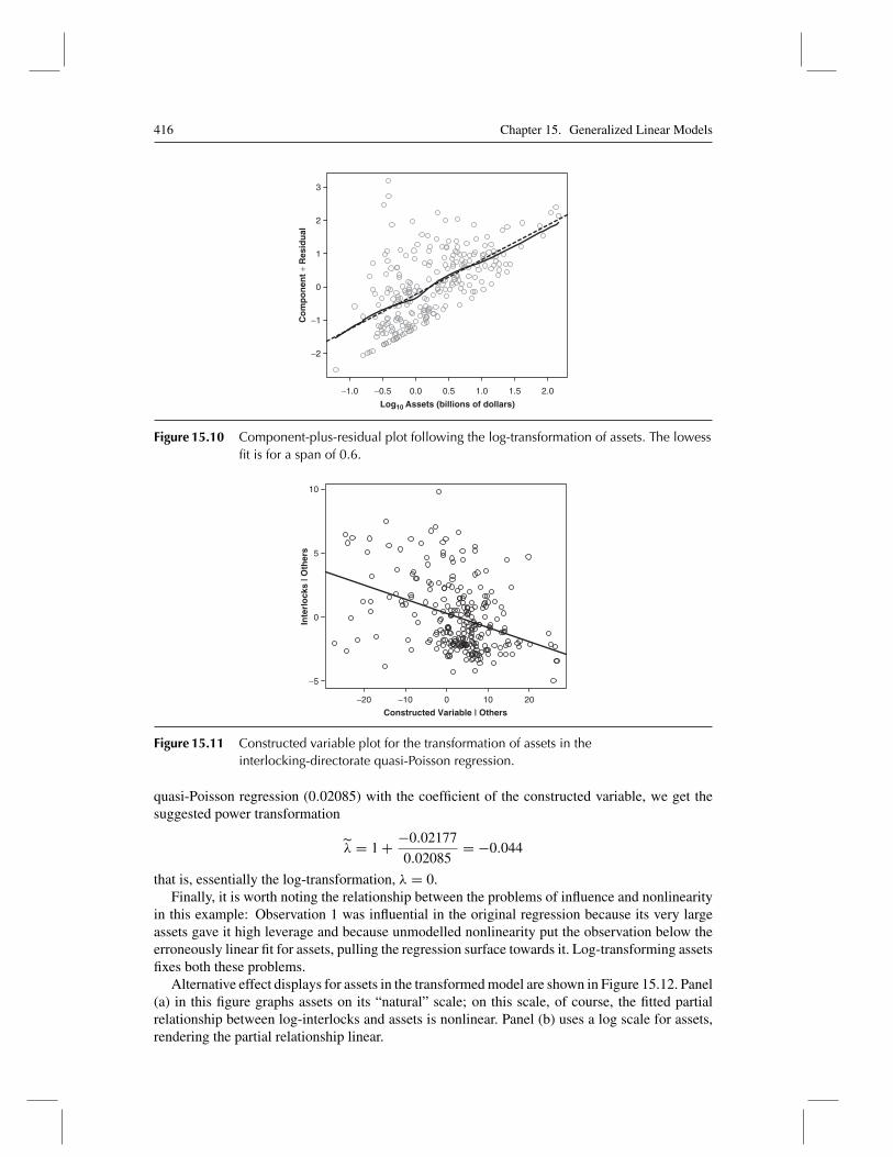
416 Chapter 15. Generalized Linear Models
−1.0 −0.5 0.0 0.5 1.0 1.5 2.0
Co
mp
on
ent
+ R
esid
ual
Log10 Assets (billions of dollars)
3
2
1
0
−1
−2
Figure 15.10 Component-plus-residual plot following the log-transformation of assets. The lowessfit is for a span of 0.6.
−20 −10 0 10 20
Constructed Variable | Others
Inte
rlo
cks
| Oth
ers 5
0
−5
10
Figure 15.11 Constructed variable plot for the transformation of assets in theinterlocking-directorate quasi-Poisson regression.
quasi-Poisson regression (0.02085) with the coefficient of the constructed variable, we get thesuggested power transformation
λ = 1 + −0.02177
0.02085= −0.044
that is, essentially the log-transformation, λ = 0.Finally, it is worth noting the relationship between the problems of influence and nonlinearity
in this example: Observation 1 was influential in the original regression because its very largeassets gave it high leverage and because unmodelled nonlinearity put the observation below theerroneously linear fit for assets, pulling the regression surface towards it. Log-transforming assetsfixes both these problems.
Alternative effect displays for assets in the transformed model are shown in Figure 15.12. Panel(a) in this figure graphs assets on its “natural” scale; on this scale, of course, the fitted partialrelationship between log-interlocks and assets is nonlinear. Panel (b) uses a log scale for assets,rendering the partial relationship linear.
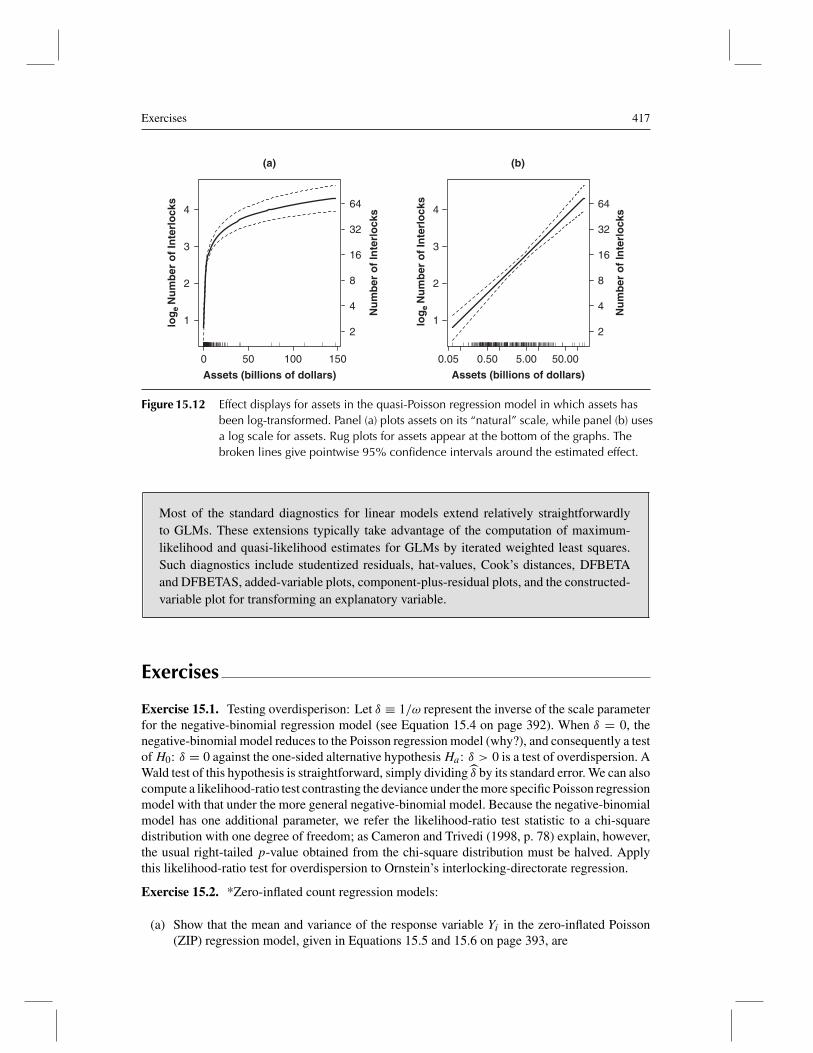
Exercises 417
0 50 100 150
(a)
Assets (billions of dollars)N
um
ber
of
Inte
rlo
cks
0.05 0.50 5.00 50.00
(b)
Assets (billions of dollars)
Nu
mb
er o
f In
terl
ock
s
log
e N
um
ber
of
Inte
rlo
cks
1
2
3
4
1
2
3
464
32
16
2
4
8
64
32
16
2
4
8
log
e N
um
ber
of
Inte
rlo
cks
Figure 15.12 Effect displays for assets in the quasi-Poisson regression model in which assets hasbeen log-transformed. Panel (a) plots assets on its “natural” scale, while panel (b) usesa log scale for assets. Rug plots for assets appear at the bottom of the graphs. Thebroken lines give pointwise 95% confidence intervals around the estimated effect.
Most of the standard diagnostics for linear models extend relatively straightforwardlyto GLMs. These extensions typically take advantage of the computation of maximum-likelihood and quasi-likelihood estimates for GLMs by iterated weighted least squares.Such diagnostics include studentized residuals, hat-values, Cook’s distances, DFBETAand DFBETAS, added-variable plots, component-plus-residual plots, and the constructed-variable plot for transforming an explanatory variable.
Exercises
Exercise 15.1. Testing overdisperison: Let δ ≡ 1/ω represent the inverse of the scale parameterfor the negative-binomial regression model (see Equation 15.4 on page 392). When δ = 0, thenegative-binomial model reduces to the Poisson regression model (why?), and consequently a testofH0: δ = 0 against the one-sided alternative hypothesisHa : δ > 0 is a test of overdispersion. AWald test of this hypothesis is straightforward, simply dividing δ by its standard error. We can alsocompute a likelihood-ratio test contrasting the deviance under the more specific Poisson regressionmodel with that under the more general negative-binomial model. Because the negative-binomialmodel has one additional parameter, we refer the likelihood-ratio test statistic to a chi-squaredistribution with one degree of freedom; as Cameron and Trivedi (1998, p. 78) explain, however,the usual right-tailed p-value obtained from the chi-square distribution must be halved. Applythis likelihood-ratio test for overdispersion to Ornstein’s interlocking-directorate regression.
Exercise 15.2. *Zero-inflated count regression models:
(a) Show that the mean and variance of the response variable Yi in the zero-inflated Poisson(ZIP) regression model, given in Equations 15.5 and 15.6 on page 393, are
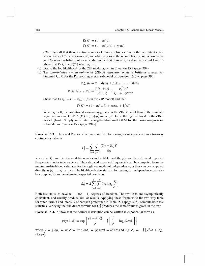
418 Chapter 15. Generalized Linear Models
E(Yi) = (1 − πi)μi
V (Yi) = (1 − πi)μi(1 + πiμi)
(Hint: Recall that there are two sources of zeroes: observations in the first latent class,whose value of Yi is necessarily 0, and observations in the second latent class, whose valuemay be zero. Probability of membership in the first class is πi , and in the second 1 − πi .)Show that V (Yi) > E(Yi) when πi > 0.
(b) Derive the log likelihood for the ZIP model, given in Equation 15.7 (page 394).(c) The zero-inflated negative-binomial (ZINB) regression model substitutes a negative-
binomial GLM for the Poisson-regression submodel of Equation 15.6 on page 393:
loge μi = α + β1xi1 + β2xi2 + · · · + βkxik
p (yi |x1, . . . , xk) = �(yi + ω)
y!�(ω)× μ
yii ω
ω
(μi + ω)μi+ω
Show that E(Yi) = (1 − πi)μi (as in the ZIP model) and that
V (Yi) = (1 − πi)μi[1 + μi(πi + 1/ω)]
When πi > 0, the conditional variance is greater in the ZINB model than in the standardnegative-binomial GLM,V (Yi) = μi+μ2
i /ω; why? Derive the log likelihood for the ZINBmodel. [Hint: Simply substitute the negative-binomial GLM for the Poisson-regressionsubmodel in Equation 15.7 (page 394)].
Exercise 15.3. The usual Pearson chi-square statistic for testing for independence in a two-waycontingency table is
X20 =
r∑i=1
c∑j=1
(Yij − μij
)2μij
where the Yij are the observed frequencies in the table, and the μij are the estimated expectedfrequencies under independence. The estimated expected frequencies can be computed from themaximum-likelihood estimates for the loglinear model of independence, or they can be computeddirectly as μij = Yi+Y+j /n. The likelihood-ratio statistic for testing for independence can alsobe computed from the estimated expected counts as
G20 = 2
r∑i=1
c∑j=1
Yij logeYij
μij
Both test statistics have (r − 1)(c − 1) degrees of freedom. The two tests are asymptoticallyequivalent, and usually produce similar results. Applying these formulas to the two-way tablefor voter turnout and intensity of partisan preference in Table 15.4 (page 395), compute both teststatistics, verifying that the direct formula for G2
0 produces the same result as given in the text.
Exercise 15.4. *Show that the normal distribution can be written in exponential form as
p(y; θ, φ) = exp
{yθ − θ2/2
φ− 1
2
[y2
φ+ loge(2πφ)
]}
where θ = gc(μ) = μ; φ = σ 2 ; a(φ) = φ; b(θ) = θ2/2; and c(y, φ) = − 12
[y2/φ + loge
(2πφ)].
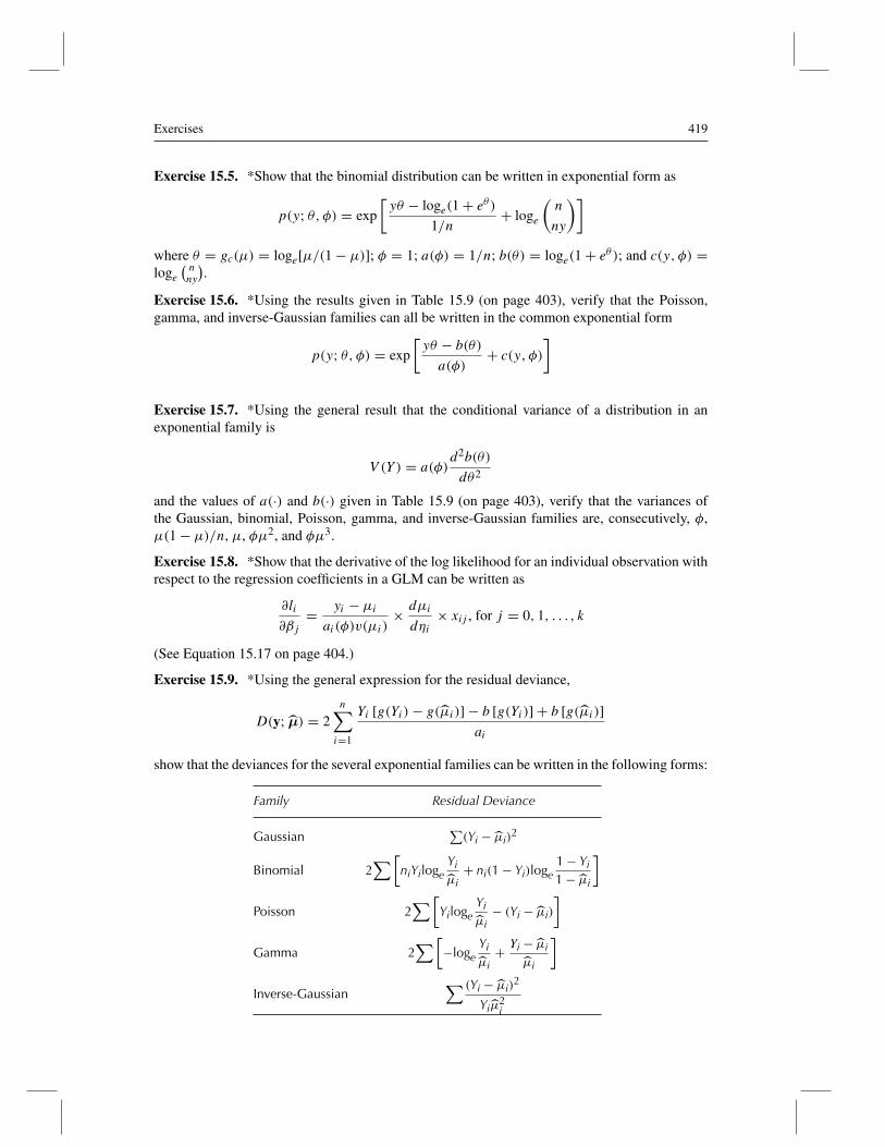
Exercises 419
Exercise 15.5. *Show that the binomial distribution can be written in exponential form as
p(y; θ, φ) = exp
[yθ − loge(1 + eθ )
1/n+ loge
(n
ny
)]
where θ = gc(μ) = loge[μ/(1 − μ)]; φ = 1; a(φ) = 1/n; b(θ) = loge(1 + eθ ); and c(y, φ) =loge
(nny
).
Exercise 15.6. *Using the results given in Table 15.9 (on page 403), verify that the Poisson,gamma, and inverse-Gaussian families can all be written in the common exponential form
p(y; θ, φ) = exp
[yθ − b(θ)
a(φ)+ c(y, φ)
]
Exercise 15.7. *Using the general result that the conditional variance of a distribution in anexponential family is
V (Y ) = a(φ)d2b(θ)
dθ2
and the values of a(·) and b(·) given in Table 15.9 (on page 403), verify that the variances ofthe Gaussian, binomial, Poisson, gamma, and inverse-Gaussian families are, consecutively, φ,μ(1 − μ)/n, μ, φμ2, and φμ3.
Exercise 15.8. *Show that the derivative of the log likelihood for an individual observation withrespect to the regression coefficients in a GLM can be written as
∂li
∂βj= yi − μi
ai(φ)v(μi)× dμi
dηi× xij , for j = 0, 1, . . . , k
(See Equation 15.17 on page 404.)
Exercise 15.9. *Using the general expression for the residual deviance,
D(y; μ) = 2n∑i=1
Yi [g(Yi)− g(μi)] − b [g(Yi)] + b [g(μi)]
ai
show that the deviances for the several exponential families can be written in the following forms:
Family Residual Deviance
Gaussian∑(Yi − μi)
2
Binomial 2∑[
niYilogeYiμi
+ ni(1 − Yi)loge1 − Yi1 − μi
]
Poisson 2∑[
YilogeYiμi
− (Yi − μi)
]
Gamma 2∑[
−logeYiμi
+ Yi − μiμi
]
Inverse-Gaussian∑ (Yi − μi)
2
Yiμ2i
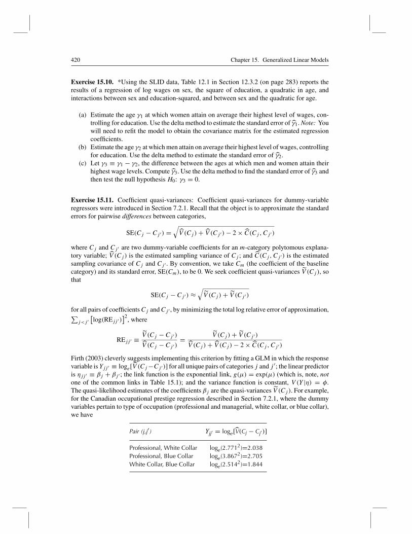
420 Chapter 15. Generalized Linear Models
Exercise 15.10. *Using the SLID data, Table 12.1 in Section 12.3.2 (on page 283) reports theresults of a regression of log wages on sex, the square of education, a quadratic in age, andinteractions between sex and education-squared, and between sex and the quadratic for age.
(a) Estimate the age γ1 at which women attain on average their highest level of wages, con-trolling for education. Use the delta method to estimate the standard error of γ1. Note: Youwill need to refit the model to obtain the covariance matrix for the estimated regressioncoefficients.
(b) Estimate the age γ2 at which men attain on average their highest level of wages, controllingfor education. Use the delta method to estimate the standard error of γ2.
(c) Let γ3 ≡ γ1 − γ2, the difference between the ages at which men and women attain theirhighest wage levels. Compute γ3. Use the delta method to find the standard error of γ3 andthen test the null hypothesis H0: γ3 = 0.
Exercise 15.11. Coefficient quasi-variances: Coefficient quasi-variances for dummy-variableregressors were introduced in Section 7.2.1. Recall that the object is to approximate the standarderrors for pairwise differences between categories,
SE(Cj − Cj ′) =√V (Cj )+ V (Cj ′)− 2 × C(Cj , Cj ′)
where Cj and Cj ′ are two dummy-variable coefficients for an m-category polytomous explana-tory variable; V (Cj ) is the estimated sampling variance of Cj ; and C(Cj , Cj ′) is the estimatedsampling covariance of Cj and Cj ′ . By convention, we take Cm (the coefficient of the baselinecategory) and its standard error, SE(Cm), to be 0. We seek coefficient quasi-variances V (Cj ), sothat
SE(Cj − Cj ′) ≈√V (Cj )+ V (Cj ′)
for all pairs of coefficientsCj andCj ′ , by minimizing the total log relative error of approximation,∑j<j ′
[log(REjj ′)
]2, where
REjj ′ ≡ V (Cj − Cj ′)
V (Cj − Cj ′)= V (Cj )+ V (Cj ′)
V (Cj )+ V (Cj )− 2 × C(Cj , Cj ′)
Firth (2003) cleverly suggests implementing this criterion by fitting a GLM in which the responsevariable is Yjj ′ ≡ loge[V (Cj−Cj ′)] for all unique pairs of categories j and j ′; the linear predictoris ηjj ′ ≡ βj + βj ′ ; the link function is the exponential link, g(μ) = exp(μ) (which is, note, notone of the common links in Table 15.1); and the variance function is constant, V (Y |η) = φ.The quasi-likelihood estimates of the coefficients βj are the quasi-variances V (Cj ). For example,for the Canadian occupational prestige regression described in Section 7.2.1, where the dummyvariables pertain to type of occupation (professional and managerial, white collar, or blue collar),we have
Pair (j,j′) Yjj′ = loge [V(Cj − Cj′)]
Professional, White Collar loge(2.7712)=2.038Professional, Blue Collar loge(3.8672)=2.705White Collar, Blue Collar loge(2.5142)=1.844
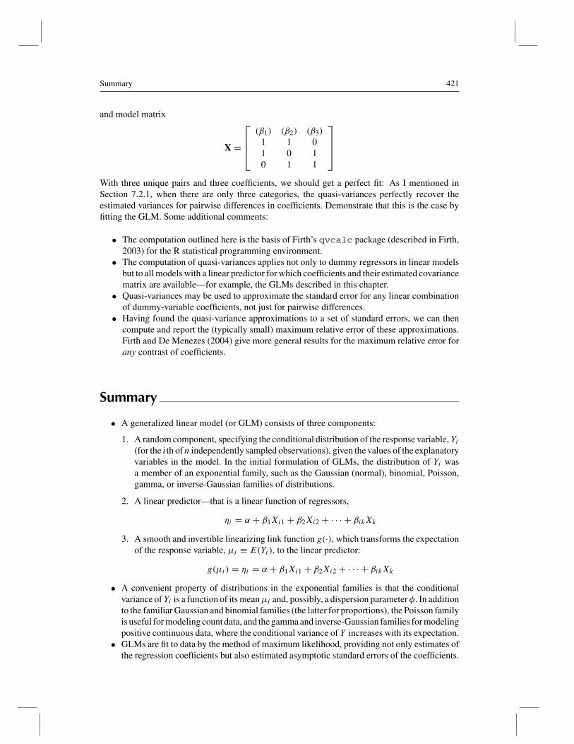
Summary 421
and model matrix
X =
⎡⎢⎢⎣(β1) (β2) (β3)
1 1 01 0 10 1 1
⎤⎥⎥⎦
With three unique pairs and three coefficients, we should get a perfect fit: As I mentioned inSection 7.2.1, when there are only three categories, the quasi-variances perfectly recover theestimated variances for pairwise differences in coefficients. Demonstrate that this is the case byfitting the GLM. Some additional comments:
• The computation outlined here is the basis of Firth’s qvcalc package (described in Firth,2003) for the R statistical programming environment.
• The computation of quasi-variances applies not only to dummy regressors in linear modelsbut to all models with a linear predictor for which coefficients and their estimated covariancematrix are available—for example, the GLMs described in this chapter.
• Quasi-variances may be used to approximate the standard error for any linear combinationof dummy-variable coefficients, not just for pairwise differences.
• Having found the quasi-variance approximations to a set of standard errors, we can thencompute and report the (typically small) maximum relative error of these approximations.Firth and De Menezes (2004) give more general results for the maximum relative error forany contrast of coefficients.
Summary
• A generalized linear model (or GLM) consists of three components:
1. A random component, specifying the conditional distribution of the response variable, Yi(for the ith of n independently sampled observations), given the values of the explanatoryvariables in the model. In the initial formulation of GLMs, the distribution of Yi wasa member of an exponential family, such as the Gaussian (normal), binomial, Poisson,gamma, or inverse-Gaussian families of distributions.
2. A linear predictor—that is a linear function of regressors,
ηi = α + β1Xi1 + β2Xi2 + · · · + βikXk
3. A smooth and invertible linearizing link function g(·), which transforms the expectationof the response variable, μi ≡ E(Yi), to the linear predictor:
g(μi) = ηi = α + β1Xi1 + β2Xi2 + · · · + βikXk
• A convenient property of distributions in the exponential families is that the conditionalvariance ofYi is a function of its meanμi and, possibly, a dispersion parameterφ. In additionto the familiar Gaussian and binomial families (the latter for proportions), the Poisson familyis useful for modeling count data, and the gamma and inverse-Gaussian families for modelingpositive continuous data, where the conditional variance of Y increases with its expectation.
• GLMs are fit to data by the method of maximum likelihood, providing not only estimates ofthe regression coefficients but also estimated asymptotic standard errors of the coefficients.
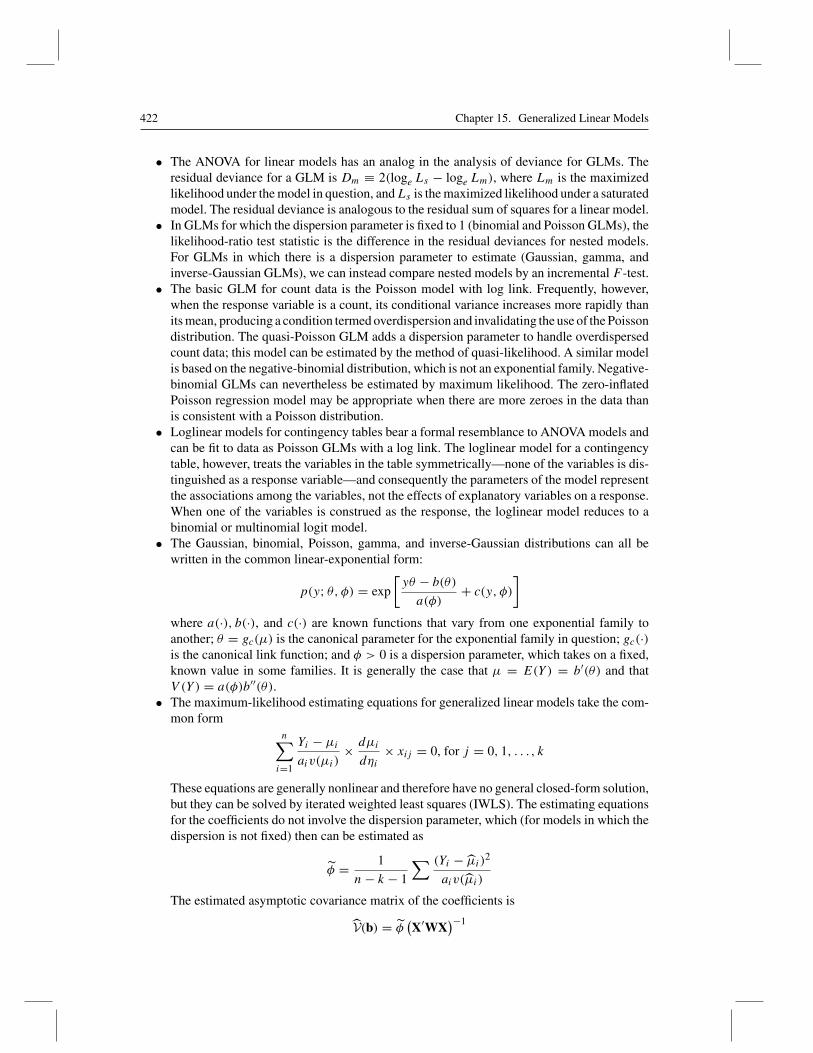
422 Chapter 15. Generalized Linear Models
• The ANOVA for linear models has an analog in the analysis of deviance for GLMs. Theresidual deviance for a GLM is Dm ≡ 2(loge Ls − loge Lm), where Lm is the maximizedlikelihood under the model in question, andLs is the maximized likelihood under a saturatedmodel. The residual deviance is analogous to the residual sum of squares for a linear model.
• In GLMs for which the dispersion parameter is fixed to 1 (binomial and Poisson GLMs), thelikelihood-ratio test statistic is the difference in the residual deviances for nested models.For GLMs in which there is a dispersion parameter to estimate (Gaussian, gamma, andinverse-Gaussian GLMs), we can instead compare nested models by an incremental F -test.
• The basic GLM for count data is the Poisson model with log link. Frequently, however,when the response variable is a count, its conditional variance increases more rapidly thanits mean, producing a condition termed overdispersion and invalidating the use of the Poissondistribution. The quasi-Poisson GLM adds a dispersion parameter to handle overdispersedcount data; this model can be estimated by the method of quasi-likelihood. A similar modelis based on the negative-binomial distribution, which is not an exponential family. Negative-binomial GLMs can nevertheless be estimated by maximum likelihood. The zero-inflatedPoisson regression model may be appropriate when there are more zeroes in the data thanis consistent with a Poisson distribution.
• Loglinear models for contingency tables bear a formal resemblance to ANOVA models andcan be fit to data as Poisson GLMs with a log link. The loglinear model for a contingencytable, however, treats the variables in the table symmetrically—none of the variables is dis-tinguished as a response variable—and consequently the parameters of the model representthe associations among the variables, not the effects of explanatory variables on a response.When one of the variables is construed as the response, the loglinear model reduces to abinomial or multinomial logit model.
• The Gaussian, binomial, Poisson, gamma, and inverse-Gaussian distributions can all bewritten in the common linear-exponential form:
p(y; θ, φ) = exp
[yθ − b(θ)
a(φ)+ c(y, φ)
]
where a(·), b(·), and c(·) are known functions that vary from one exponential family toanother; θ = gc(μ) is the canonical parameter for the exponential family in question; gc(·)is the canonical link function; and φ > 0 is a dispersion parameter, which takes on a fixed,known value in some families. It is generally the case that μ = E(Y ) = b′(θ) and thatV (Y ) = a(φ)b′′(θ).
• The maximum-likelihood estimating equations for generalized linear models take the com-mon form
n∑i=1
Yi − μi
aiv(μi)× dμi
dηi× xij = 0, for j = 0, 1, . . . , k
These equations are generally nonlinear and therefore have no general closed-form solution,but they can be solved by iterated weighted least squares (IWLS). The estimating equationsfor the coefficients do not involve the dispersion parameter, which (for models in which thedispersion is not fixed) then can be estimated as
φ = 1
n− k − 1
∑ (Yi − μi)2
aiv(μi)
The estimated asymptotic covariance matrix of the coefficients is
V(b) = φ(X′WX
)−1
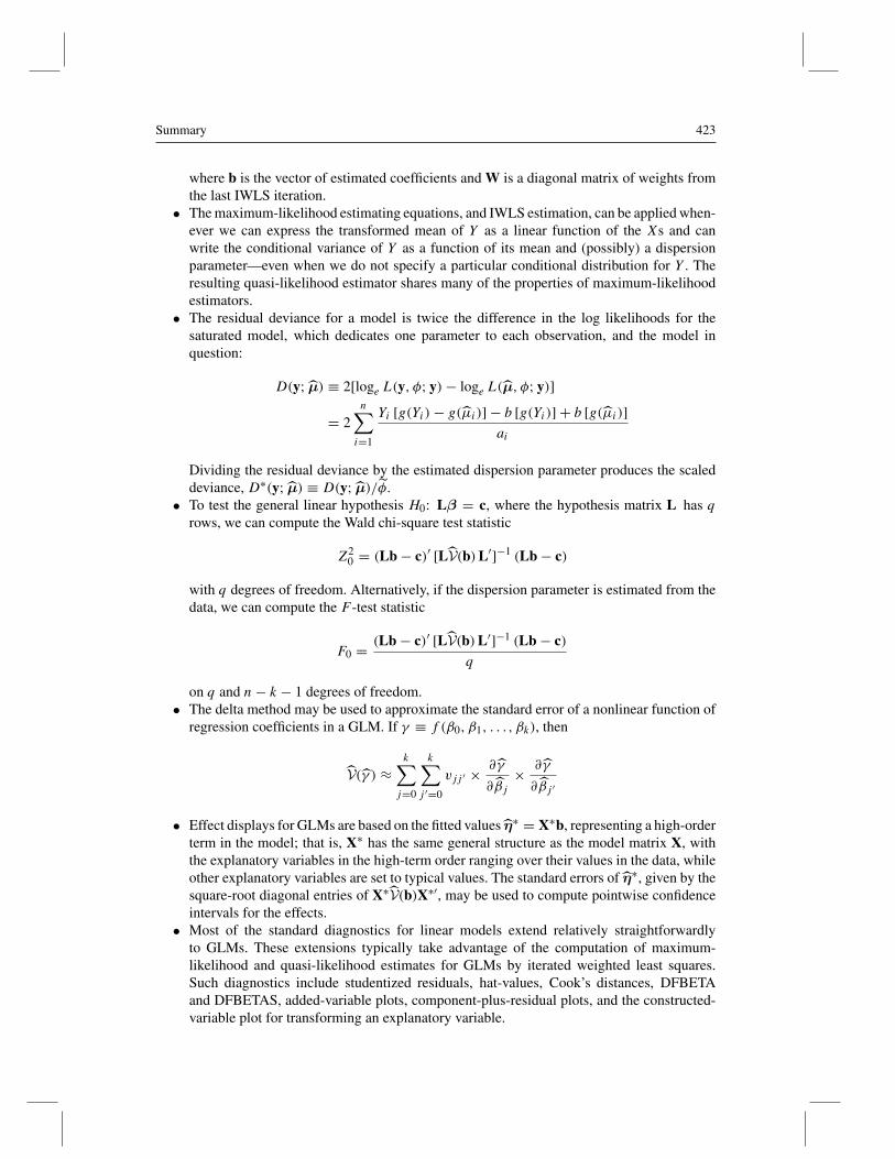
Summary 423
where b is the vector of estimated coefficients and W is a diagonal matrix of weights fromthe last IWLS iteration.
• The maximum-likelihood estimating equations, and IWLS estimation, can be applied when-ever we can express the transformed mean of Y as a linear function of the Xs and canwrite the conditional variance of Y as a function of its mean and (possibly) a dispersionparameter—even when we do not specify a particular conditional distribution for Y . Theresulting quasi-likelihood estimator shares many of the properties of maximum-likelihoodestimators.
• The residual deviance for a model is twice the difference in the log likelihoods for thesaturated model, which dedicates one parameter to each observation, and the model inquestion:
D(y; μ) ≡ 2[loge L(y, φ; y)− loge L(μ, φ; y)]
= 2n∑i=1
Yi [g(Yi)− g(μi)] − b [g(Yi)] + b [g(μi)]
ai
Dividing the residual deviance by the estimated dispersion parameter produces the scaleddeviance, D∗(y; μ) ≡ D(y; μ)/φ.
• To test the general linear hypothesis H0: Lβ = c, where the hypothesis matrix L has qrows, we can compute the Wald chi-square test statistic
Z20 = (Lb − c)′ [LV(b)L′]−1 (Lb − c)
with q degrees of freedom. Alternatively, if the dispersion parameter is estimated from thedata, we can compute the F -test statistic
F0 = (Lb − c)′ [LV(b)L′]−1 (Lb − c)q
on q and n− k − 1 degrees of freedom.• The delta method may be used to approximate the standard error of a nonlinear function of
regression coefficients in a GLM. If γ ≡ f (β0, β1, . . . , βk), then
V(γ ) ≈k∑j=0
k∑j ′=0
vjj ′ × ∂γ
∂βj× ∂γ
∂βj ′
• Effect displays for GLMs are based on the fitted values η∗ = X∗b, representing a high-orderterm in the model; that is, X∗ has the same general structure as the model matrix X, withthe explanatory variables in the high-term order ranging over their values in the data, whileother explanatory variables are set to typical values. The standard errors of η∗, given by thesquare-root diagonal entries of X∗V(b)X∗′, may be used to compute pointwise confidenceintervals for the effects.
• Most of the standard diagnostics for linear models extend relatively straightforwardlyto GLMs. These extensions typically take advantage of the computation of maximum-likelihood and quasi-likelihood estimates for GLMs by iterated weighted least squares.Such diagnostics include studentized residuals, hat-values, Cook’s distances, DFBETAand DFBETAS, added-variable plots, component-plus-residual plots, and the constructed-variable plot for transforming an explanatory variable.

424 Chapter 15. Generalized Linear Models
Recommended Reading
• McCullagh and Nelder (1989), the “bible” of GLMs, is a rich and interesting—if generallydifficult—text.
• Dobson (2001) presents a much briefer overview of generalized linear models at a moremoderate level of statistical sophistication.
• Aitkin, Francis, and Hinde’s (2005) text, geared to the statistical computer package GLIMfor fitting GLMs, is still more accessible.
• A chapter by Firth (1991) is the best brief treatment of generalized linear models that I haveread.
• Long (1997) includes an excellent presentation of regression models for count data (thoughnot from the point of view of GLMs); an even more extensive treatment may be found inCameron and Trivedi (1998).


