Evidence Based Investing is Dead. Long LiveEvidence Based Investing! Part 1

September 25, 2017by Adam Butler

Advisor Perspectives welcomes guest contributions. The views presented here do not necessarilyrepresent those of Advisor Perspectives.

Michael Edesess’ article, The Trend that is Ruining Finance Research, makes the case that financialresearch is flawed. In this two-part article series, I will examine the points that Edesess raised in somedetail. His arguments have some merit. Importantly however, his article fails to undermine the value offinance research in general. Rather, his points serve to highlight that finance is a real profession thatrequires skills, education, and experience that differentiates professionals from laymen.

Edesess’ case against evidence-based inveesting rests on three general assertions. There is a veryreal issue with using a static t-statistic threshold when the number of independent tests becomes verylarge. Financial research is often conducted with a universe of securities that includes a large numberof micro-cap and nano-cap stocks. These stocks often do not trade regularly, and exhibit largeovernight jumps in prices. They are also illiquid and costly to trade. Third, the regression models usedin most financial research are poorly calibrated to form conclusions on non-stationary financial datawith large outliers.

This article will explore the issues around the latter two challenges. My next article will tackle the “p-hacking” issue in finance, and propose a framework to help those who embrace evidence-basedinvesting to make judicious decisions based on a more thoughtful interpretation of finance research.

An un-investable investment universe

A large proportion of finance studies perform their analysis with a universe of stocks that is practicallyun-investable for most investors. That’s because they include stocks with very small marketcapitalizations. In fact, the top 1,000 stocks by market capitalization represent over 93% of the totalaggregate market capitalization of all U.S. stocks. This means the bottom 3,000 or so stocks accountfor just 7% of total market capitalization. The median market cap of a stock in the bottom half of themarket capitalization distribution is just over $1billion.

Figure 1. Cumulative proportion of U.S. market capitalization

Page 1, ©2018 Advisor Perspectives, Inc. All rights reserved.

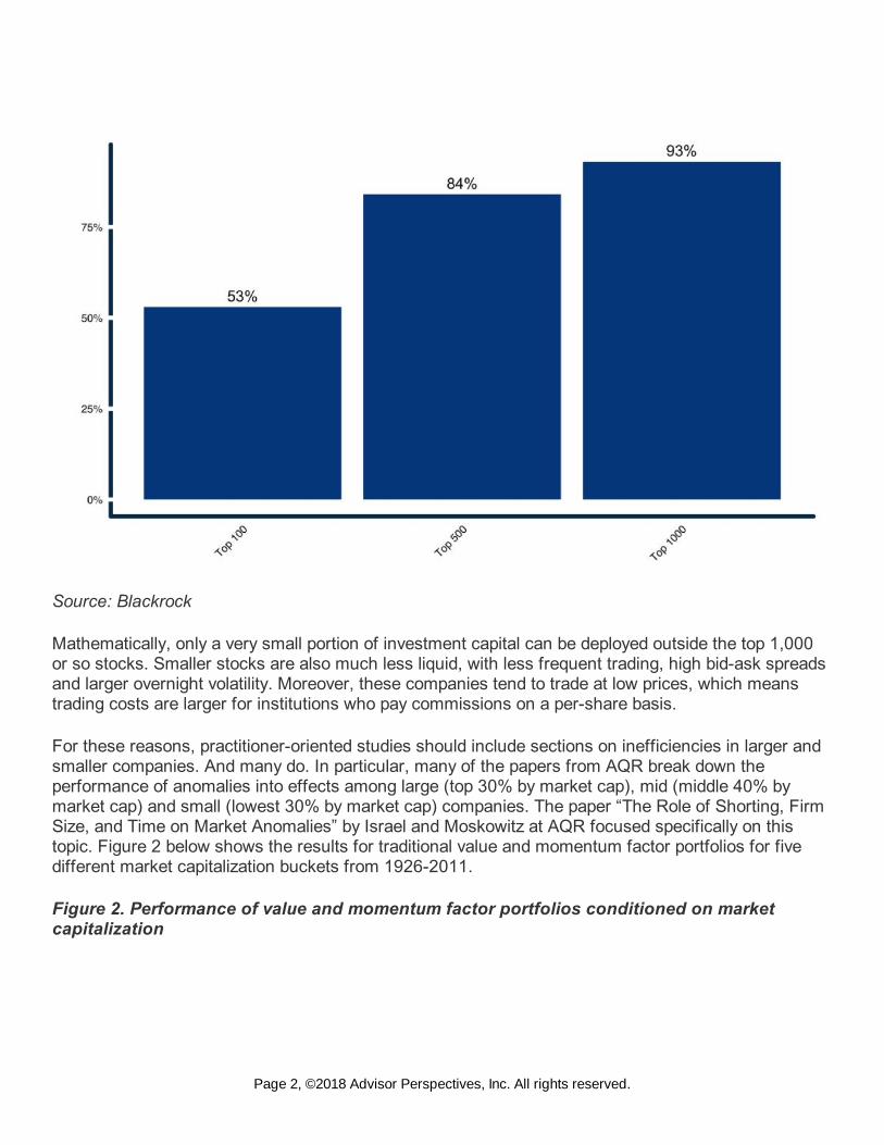
Source: Blackrock

Mathematically, only a very small portion of investment capital can be deployed outside the top 1,000or so stocks. Smaller stocks are also much less liquid, with less frequent trading, high bid-ask spreadsand larger overnight volatility. Moreover, these companies tend to trade at low prices, which meanstrading costs are larger for institutions who pay commissions on a per-share basis.

For these reasons, practitioner-oriented studies should include sections on inefficiencies in larger andsmaller companies. And many do. In particular, many of the papers from AQR break down theperformance of anomalies into effects among large (top 30% by market cap), mid (middle 40% bymarket cap) and small (lowest 30% by market cap) companies. The paper “The Role of Shorting, FirmSize, and Time on Market Anomalies” by Israel and Moskowitz at AQR focused specifically on thistopic. Figure 2 below shows the results for traditional value and momentum factor portfolios for fivedifferent market capitalization buckets from 1926-2011.

Figure 2. Performance of value and momentum factor portfolios conditioned on marketcapitalization

Page 2, ©2018 Advisor Perspectives, Inc. All rights reserved.

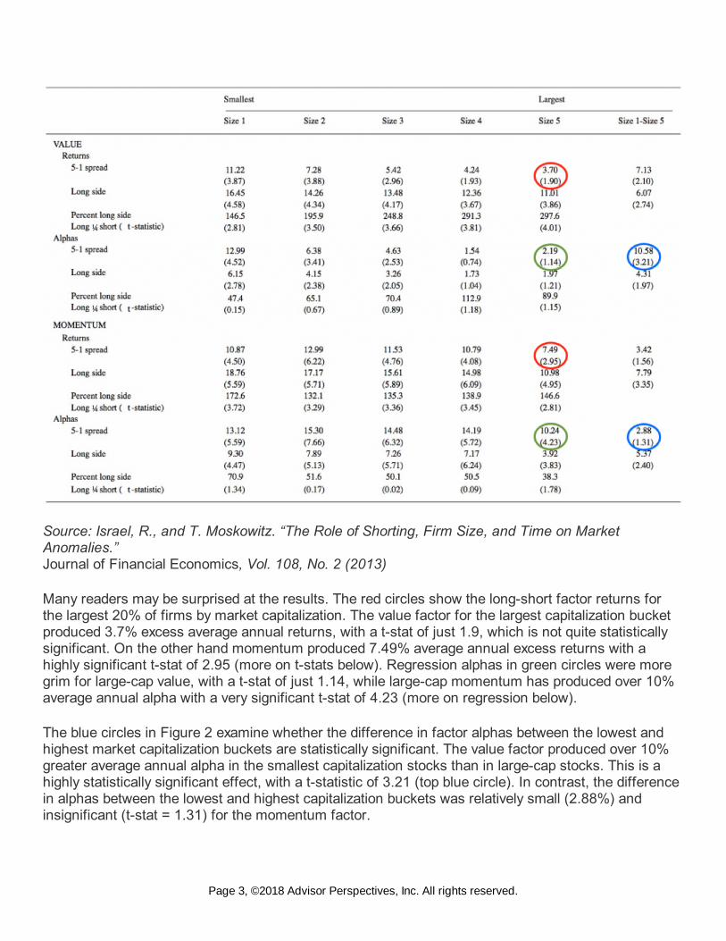
Source: Israel, R., and T. Moskowitz. “The Role of Shorting, Firm Size, and Time on MarketAnomalies.” Journal of Financial Economics, Vol. 108, No. 2 (2013)

Many readers may be surprised at the results. The red circles show the long-short factor returns forthe largest 20% of firms by market capitalization. The value factor for the largest capitalization bucketproduced 3.7% excess average annual returns, with a t-stat of just 1.9, which is not quite statisticallysignificant. On the other hand momentum produced 7.49% average annual excess returns with ahighly significant t-stat of 2.95 (more on t-stats below). Regression alphas in green circles were moregrim for large-cap value, with a t-stat of just 1.14, while large-cap momentum has produced over 10%average annual alpha with a very significant t-stat of 4.23 (more on regression below).

The blue circles in Figure 2 examine whether the difference in factor alphas between the lowest andhighest market capitalization buckets are statistically significant. The value factor produced over 10%greater average annual alpha in the smallest capitalization stocks than in large-cap stocks. This is ahighly statistically significant effect, with a t-statistic of 3.21 (top blue circle). In contrast, the differencein alphas between the lowest and highest capitalization buckets was relatively small (2.88%) andinsignificant (t-stat = 1.31) for the momentum factor.

Page 3, ©2018 Advisor Perspectives, Inc. All rights reserved.

The analysis in Figure 2 did not account for trading frictions. After accounting for the cost of liquidity,which might be substantial for small-cap stocks, but inconsequential for large-cap stocks, the gapbetween large- and small-cap factor performance would almost certainly close, perhaps significantly. Inaddition, those practitioners who are fond of small- or mid-cap value should feel well validated, asvalue-factor performance is strong and significant for every market capitalization quintile other than thelargest cap stocks.

Investors must be aware of the practical implications of the universe chosen for investment research.Practitioners should focus on observed effects among mid- and large-capitalization stocks, whereresults align more closely with academic findings.

Regression is a blunt tool

Researchers in empirical finance use linear regression to determine whether, and to what extent, aneffect that they are investigating is already explained by previously documented effects. For example,academics use linear regression to determine how well a factor model explains differences in thecross-section of securities prices. Researchers in search of novel return premia use linear regressionto determine how much value a newly proposed factor adds above what is explained by already well-known factors. Advisors, consultants and investors use regression to determine if an active investmentproduct or strategy has delivered significant excess risk-adjusted performance, above what they couldachieve through inexpensive exposure to factor products.

Unfortunately, linear regression is a very blunt tool when it comes to dealing with complex financialdata. The following example will highlight one important reason why. I poached this example from LarrySwedroe's great book, Reducing the Risk of Black Swans (update forthcoming), because it is soperfect and surprising.

Consider two strategies A and B, and their returns over a 10-year period. Their return series is depictedin the table below.

Period 1

StrategyYear 1Year 2Year 3Year 4Year 5Year 6Year 7Year 8Year 9Year 10

A 12% 8% 12% 8% 12% 8% 12% 8% 12% 8%

B 8% 12% 8% 12% 8% 12% 8% 12% 8% 12%

Both strategies have an annual average return of 10%. Whenever A’s return is above its average of10%, B’s return is below its average of 10%. And whenever A’s return is below its average of 10, B’sreturn is above its average of 10%. Thus, regressing strategy A’s returns on strategy B’s returns overthis period will conclude that they are negatively correlated. Note that they are negatively correlatedeven though they both always produced positive returns.

Now imagine that the same strategies produced the following returns in a different 10-year period.

Page 4, ©2018 Advisor Perspectives, Inc. All rights reserved.

Period 2

StrategyYear 1Year 2Year 3Year 4Year 5Year 6Year 7Year 8Year 9Year 10

A 2 -2 2 -2 2 -2 2 -2 2 -2

B -2 2 -2 2 -2 2 -2 2 -2 2

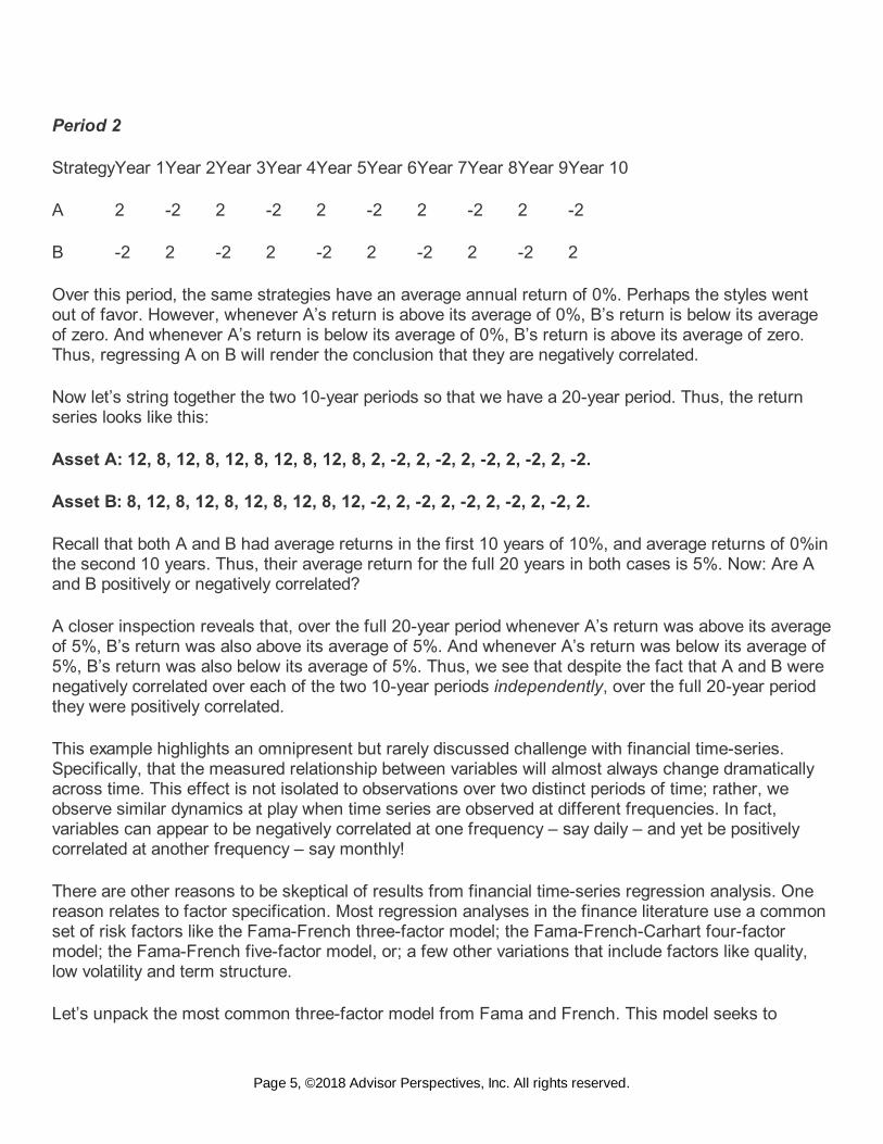
Over this period, the same strategies have an average annual return of 0%. Perhaps the styles wentout of favor. However, whenever A’s return is above its average of 0%, B’s return is below its averageof zero. And whenever A’s return is below its average of 0%, B’s return is above its average of zero.Thus, regressing A on B will render the conclusion that they are negatively correlated.

Now let’s string together the two 10-year periods so that we have a 20-year period. Thus, the returnseries looks like this:

Asset A: 12, 8, 12, 8, 12, 8, 12, 8, 12, 8, 2, -2, 2, -2, 2, -2, 2, -2, 2, -2.

Asset B: 8, 12, 8, 12, 8, 12, 8, 12, 8, 12, -2, 2, -2, 2, -2, 2, -2, 2, -2, 2.

Recall that both A and B had average returns in the first 10 years of 10%, and average returns of 0%inthe second 10 years. Thus, their average return for the full 20 years in both cases is 5%. Now: Are Aand B positively or negatively correlated?

A closer inspection reveals that, over the full 20-year period whenever A’s return was above its averageof 5%, B’s return was also above its average of 5%. And whenever A’s return was below its average of5%, B’s return was also below its average of 5%. Thus, we see that despite the fact that A and B werenegatively correlated over each of the two 10-year periods independently, over the full 20-year periodthey were positively correlated.

This example highlights an omnipresent but rarely discussed challenge with financial time-series.Specifically, that the measured relationship between variables will almost always change dramaticallyacross time. This effect is not isolated to observations over two distinct periods of time; rather, weobserve similar dynamics at play when time series are observed at different frequencies. In fact,variables can appear to be negatively correlated at one frequency – say daily – and yet be positivelycorrelated at another frequency – say monthly!

There are other reasons to be skeptical of results from financial time-series regression analysis. Onereason relates to factor specification. Most regression analyses in the finance literature use a commonset of risk factors like the Fama-French three-factor model; the Fama-French-Carhart four-factormodel; the Fama-French five-factor model, or; a few other variations that include factors like quality,low volatility and term structure.

Let’s unpack the most common three-factor model from Fama and French. This model seeks to

Page 5, ©2018 Advisor Perspectives, Inc. All rights reserved.

explain returns using a combination of a market factor (MKT), a size factor (SMB) and a value factor(HML). Fama and French define the value factor using the book-to-price ratio. Specifically, each July31st they sort stocks based on the book-to-price ratio observed on December 31st of the previous year.So when a value-oriented investment strategy is regressed with the three-factor model, if the strategyemploys the book-to-price ratio, and rebalances on the same dates as the value strategy in the FamaFrench model, the regression will show a strong value tilt .

However, “value” can be defined in many ways. Some practitioners use book-to-price; others useearnings-to-price, sales-to-price or cash-flow-to-price, or other metrics. Portfolios have differentnumbers of holdings and are rebalanced at different times. Many managers use several factors at onceto measure value. All of these deviations from the traditional value factor specification will lead theregression model to observe weak exposure to the “value” factor, even though the other valuespecifications and methods are equally useful.

The AQR Alternative Style Premia Fund (QSPIX) offers an informative case study. The fund purportsto invest in pure, market-neutral value, momentum, carry, and “defensive” factor strategies applied toindividual stocks and bonds, as well as stock and bond indexes and other asset classes around theworld.

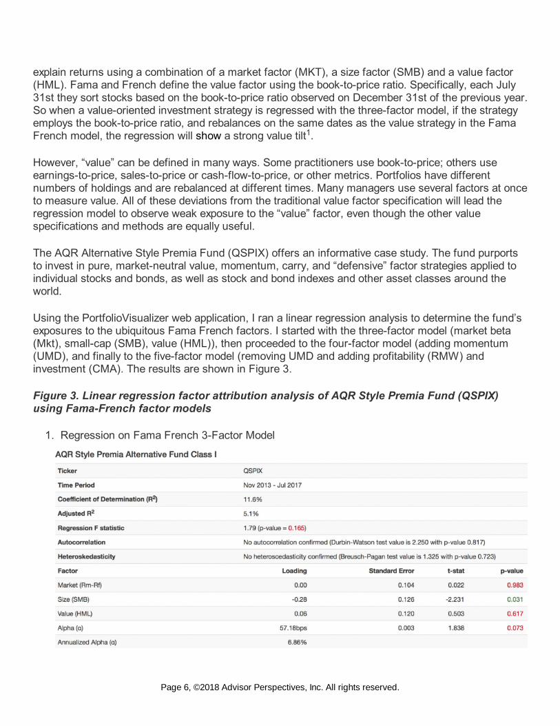
Using the PortfolioVisualizer web application, I ran a linear regression analysis to determine the fund’sexposures to the ubiquitous Fama French factors. I started with the three-factor model (market beta(Mkt), small-cap (SMB), value (HML)), then proceeded to the four-factor model (adding momentum(UMD), and finally to the five-factor model (removing UMD and adding profitability (RMW) andinvestment (CMA). The results are shown in Figure 3.

Figure 3. Linear regression factor attribution analysis of AQR Style Premia Fund (QSPIX)using Fama-French factor models

1. Regression on Fama French 3-Factor Model

1

Page 6, ©2018 Advisor Perspectives, Inc. All rights reserved.

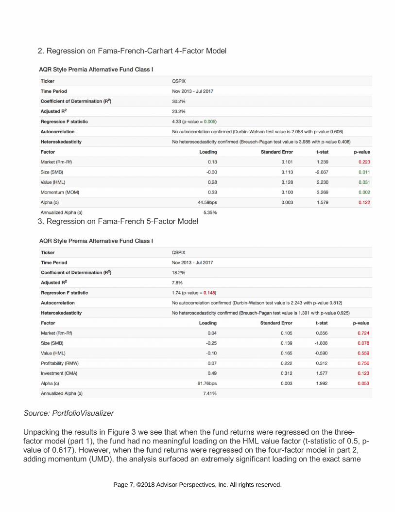
2. Regression on Fama-French-Carhart 4-Factor Model

3. Regression on Fama-French 5-Factor Model

Source: PortfolioVisualizer

Unpacking the results in Figure 3 we see that when the fund returns were regressed on the three-factor model (part 1), the fund had no meaningful loading on the HML value factor (t-statistic of 0.5, p-value of 0.617). However, when the fund returns were regressed on the four-factor model in part 2,adding momentum (UMD), the analysis surfaced an extremely significant loading on the exact same

Page 7, ©2018 Advisor Perspectives, Inc. All rights reserved.

value factor, along with a very significant loading on momentum. Then when momentum was replacedwith profitability and investment factors in part 3, value disappears again. In fact, the fund returnsappear not to load meaningfully on any of the factors!

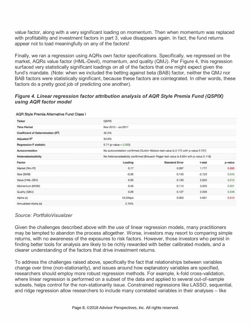
Finally, we ran a regression using AQRs own factor specifications. Specifically, we regressed on themarket, AQRs value factor (HML-Devil), momentum, and quality (QMJ). Per Figure 4, this regressionsurfaced very statistically significant loadings on all of the factors that one might expect given thefund’s mandate. (Note: when we included the betting against beta (BAB) factor, neither the QMJ norBAB factors were statistically significant, because these factors are cointegrated. In other words, thesefactors do a pretty good job of predicting one another).

Figure 4. Linear regression factor attribution analysis of AQR Style Premia Fund (QSPIX)using AQR factor model

Source: PortfolioVisualizer

Given the challenges described above with the use of linear regression models, many practitionersmay be tempted to abandon the process altogether. Worse, investors may resort to comparing simplereturns, with no awareness of the exposures to risk factors. However, those investors who persist infinding better tools for analysis are likely to be richly rewarded with better calibrated models, and aclearer understanding of the factors that drive investment returns.

To address the challenges raised above, specifically the fact that relationships between variableschange over time (non-stationarity), and issues around how explanatory variables are specified,researchers should employ more robust regression methods. For example, k-fold cross-validation,where linear regression is performed on a subset of the data and applied to several out-of-samplesubsets, helps control for the non-stationarity issue. Constrained regressions like LASSO, sequential,and ridge regression allow researchers to include many correlated variables in their analyses – like

Page 8, ©2018 Advisor Perspectives, Inc. All rights reserved.

different specifications of “value,” or both the QMJ and BAB factors – which would otherwise corrupt alinear regression analysis.

Admittedly, these tools require technical knowledge and advanced education, but such is the nature ofa true profession. Professionals have a responsibility to evolve and improve their methods when facedwith the fact that the old tools are inadequate. Those who wish to learn more about these methodscould do a lot worse than this book.

Summary

Finance research suffers from a variety of challenges that make it difficult for practitioners to makeinformed decisions. Many papers include in their analysis stocks with very small market capitalizations,which would not be tradable in practice. When the same studies are conducted on larger capitalizationstocks, which investors could trade with reasonable costs and scale, researchers often arrive atdifferent results. I highlighted one example, which showed that, while the popular “value” factor exhibitsa large and significant effect when applied to mid- and small-cap U.S. companies, it renders astatistically insignificant result when applied to a large-cap investment universe. Thus there is littlevalue in exposing investors to value tilts in large-cap portfolios.

Another important consideration for evidence-based investors is that the most common tool forinvestigation – linear regression – is not well designed to deal with noisy and evolving financial data. Asa case study, I performed several factor attribution regression analyses on a pure factor-orientedproduct, the AQR Alt Premia Fund (QSPIX). My results show that these types of regression analysesare highly sensitive to which factors are included as explanatory variables, and how those factors arespecified. I suggested several advanced regression methods that address the key challenges oftraditional regression analysis, but warned that meaningful research will require a greater depth ofknowledge about advanced statistical techniques.

In my next article, I will explore the issue of scalability in financial research. Advances in computationalpower and an explosion of new data sources makes it easy to test thousands of potential relationshipsamong financial variables. Just as a billion monkeys typing randomly for thousands of years willeventually produce a Shakespearean sonnet, thousands of researchers running tests on millions ofcombinations of economic variables will inevitably stumble onto spurious relationships. I take this issuehead-on, and show that the most robust factors easily survive this statistical challenge. I also propose aframework to help investment professionals make judicious decisions based on finance research.

Adam Butler, CFA, CAIA, is co-founder and chief investment officer of ReSolve Asset Management.ReSolve manages funds and accounts in Canada, the United States and internationally.

1 Fama and French performed other machinations to create their factor portfolios which confoundregression analysis for attribution on real investment strategies. For example, to create the value factorreturns they perform the sort on large cap stocks, and again on small-cap stocks, and average theresults from the two sorts.

Page 9, ©2018 Advisor Perspectives, Inc. All rights reserved.