Download - Copulas in Macroeconomics - Southeastern Louisiana …...Copulas in Macroeconomics . Kevin Dowd* Centre for Risk and Insurance Studies . Nottingham University Business School . Abstract

Dowd, Journal of International and global Economic Studies, 1(1), June 2008, 1-26 1

Copulas in Macroeconomics

Kevin Dowd*

Centre for Risk and Insurance Studies Nottingham University Business School

Abstract This paper discusses the uses of copulas for modelling multivariate density functions and explains how copula methods can be applied to the study of macroeconomic relationships. It suggests that copulas are well suited to the study of these relationships and can sometimes shed new light on them. It then sets out the main steps of copula methodology and provides an illustrative application to the phenomenon of the Gibson paradox. Keywords: Copulas, macroeconomics, correlations JEL Classification: C10, C49, E17

1. Introduction Much of applied macroeconomics is concerned with the analysis of relationships between macroeconomic variables. Typically, analysis is carried out using some form of conditional modelling (e.g., regression) in which the relationship is expressed in terms of a variable being conditional on one or more others. However, at a very general level, all multivariate analysis can be represented in terms of multivariate distribution functions, conditional or otherwise. This paper suggests a different and in some respects superior approach to multivariate relationships based on copula functions.1 A copula provides an alternative way of representing a multivariate density function. Indeed, copulas have been described as the “fundamental building blocks for studying multivariate distributions” (Frees and Valdez (1998, p. 3)). The main attraction of a copula approach is that it enables us to model the dependence structure of a multivariate distribution separately from the marginal distribution functions of the individual random variables. This ability to ‘separate’ the dependence structure from the marginals makes for much greater modelling flexibility than is possible with traditional approaches to multivariate problems. Copula approaches have been used in various areas of applied statistics with considerable success. Closer to home, they have been used for a number of years in actuarial science, and are now making major inroads into applied finance. In the actuarial field, they have been applied to such problems as bivariate survival analysis, loss modelling, and the analysis of indemnity claims (see, e.g., Frees and Valdez (1998)). In finance, they have been applied to the modelling of financial returns (e.g., Ang and Chen (2002), Chen et alia (2004), Patton (2002, 2004), Rodriguez (2003), and Rockinger and Jondeau (2004)), the modeling of multivariate high-frequency data (e.g., Breymann et alia (2003)), pricing options with multiple underlying


variables (e.g., Cherubini and Luciano (2002) and Goorbergh et alia (2005)), modelling the probabilities of multiple defaults in credit portfolios (e.g., Li (2000)), and the estimation of Value at Risk (e.g., Cherubini and Luciano (2001) and Ané and Kharoubi (2003)).2 This paper suggests that copula methods are well suited to the study of many macroeconomic relationships.3 This is partly because hypotheses about such relationships can often be expressed in terms of hypotheses about the correlations between two (or maybe more) random variables. These hypotheses sometimes involve some form of conditionality, and sometimes relate to the noise or error process in macroeconomic equations. Hypotheses about unconditional correlations arise in the quantity theory of money, the Fisher effect, earlier versions of the Philips curve, the Gibson paradox, and elsewhere in macroeconomics (e.g., the relationship between productivity growth and inflation; see Kiley (2003)). Examples of conditional correlations arise for instance with the expectations-augmented Philips curve (where the correlation is conditional on expected inflation).4 The expectations-augmented Philips curve can also be regarded as an example of a macroeconomic hypothesis regarding a noise process (since it postulates that the shock to inflation should be positively associated with output or an output shock). The major macroeconomic behavioral functions (consumptions functions, demand-for-money functions, etc.) can also be expressed in similar terms. Indeed, any conditional relationship can be expressed in such terms. It is also important to appreciate that copulas can do more than merely shed light on correlations. Since copulas enable us to model the multivariate density function, they shed light on the complete relationship, of which any correlation only gives us a partial picture. For instance, a copula analysis might show how the relevant variables are related in their tails, as well as in their central masses. Thus, a copula analysis is able to provide more insight into the phenomenon involved, and is not restricted to an analysis of correlations alone. This paper is organized as follows. Section 2 provides a brief overview of relevant copula theory and how it can be implemented in a macroeconomic context. Section 3 discusses methodology. Section 4 then illustrates the macroeconomic potential of copulas with a copula-based analysis of a well-known macroeconomic relationship, the Gibson paradox under gold standard. Section 5 concludes.

2. Copulas

2.1. Introduction to Copulas The key to copulas is the Sklar theorem (Sklar (1959)). Given two random variables X and Y with continuous marginals and uxFx =)( vyFy =)( , this theorem tells us that their joint distribution function can be written in terms of a unique function : ),( yxF ),( vuC

),(),( vuCyxF = (1)


The function is known as the copula of , and describes how is coupled with the marginal distribution functions and . A copula is thus a function that ‘joins together’ a collection of marginal distributions to form a multivariate distribution. It can also be interpreted as representing the dependence structure of

),( vuC ),( yxF)(yFy

),( yxF)(xFx

X and Y . 2.2. Advantages of Copulas Copula approaches to the modelling of multivariate density functions have a number of advantages over traditional approaches based on the representation of such probabilities: ),( yxF

• Copulas are much more flexible, because they allow us to fit the dependence structure separately from the marginal distributions. This is superior as a modelling strategy, especially in situations (which are also common in macroeconomics) where it is the dependence structure that we are mostly interested in.5 With traditional ),( yxF representations, by contrast, we cannot (typically) ‘get at’ the dependence structure without also having to make (often unwanted and unwarranted) assumptions about marginal distributions,6 and there is the related problem that dependence parameters are sometimes present in the marginals.

• The fact that copulas allow us to separate the modelling of dependence from the

modelling of the marginals allows us to fit different marginal distributions to different random variables. By comparison, traditional approaches (typically) require us to fit the same marginals to all random variables. The greater flexibility afforded by copula approaches is often of tremendous value, as empirical marginal distributions can often be very different from each other.

• Copula approaches also make for greater flexibility because they give us much greater

choice over the type of dependence structure that we can fit to our data. With copulas, we can fit any type of dependence structure that is achievable using traditional ),( yxF representations of the multivariate density function, but we can also fit many more (e.g., such as the Archimedean copulas considered next).

Put bluntly, with copulas we can do anything we can already do with traditional methods (e.g., we can still model conditional and time-dependent relationships, etc.), but we can also do a great deal more. 2.3. Archimedean Copulas The copulas examined in this paper are the Archimedean copulas.7 These are a family of copulas that can be written in the form:

)]()([),( 1 vuvuC φφφ += − (2) for some convex decreasing function (.)φ defined over (0,1] such that 0)1( =φ . The function

(.)φ is known as the generator of the copula, and depends on a single parameter α that reflects


the degree of dependence. Archimedean copulas allow a wide range of possible dependence behavior, have attractive mathematical and statistical properties and are very convenient and tractable (see, e.g., Genest and Rivest (1993)).8 The choice of generator determines the copula, and we consider three copulas in the Archimedean family. These are the Clayton, Frank and Gumbel copulas, whose copulas and generators are given in Table 1. Archimedean copulas are convenient in part because the copula parameter α is closely related to the Kendall’s τ coefficient of correlation, defined as follows:

∑∑= >

−−−

=n

i ijjiji YYXX

nn 1))(sgn(

)1(2τ (3)

where ‘sgn’ refers to the sign of the term that follows it. The τ has some nice properties,9 and Genest and MacKay (1986, p. 283) show that the relationship between α and τ is given by:

1)(')(4

1

0

+= ∫ dttt

φφτ . (4)

This relationship allows us to recover an estimate of α from one of τ using a suitable equation or algorithm that depends on the copula. Since τ is easily estimated, this means that estimates of α are straightforward to obtain.10 We can also identify the best-fitting Archimedean copula using a method suggested by Genest and Rivest (1993). To do so, we define the latent variable , the value of the copula function, as

and denote its distribution function by . This distribution function is related to the generator of an Archimedean copula by the following relationship (due to Genest and Rivest (1993, pp. 1034-1036)):

iZ)z),( iii YXFZ = (K

)(')()(

zzzzK

φφ

−= (5)

This relationship allows us to identify from knowledge of the copula generator and of the parameter

)(zKα . Now define the non-parametric version of , , as follows: )(zK )(ˆ zK

nzZI

zKn

i i∑ =<

= 1)ˆ(

)(ˆ (6)

where is the indicator function (which takes the value 1 if the specified condition is met, and otherwise takes the value 0) and is the empirical analogue of , i.e.,

(.)I

iZ iZ


=iZ #1

},:),{(−

<<

nYYXXYX ijijjj (7)

for , where the symbol indicates ‘#’ that we count the number of observations that satisfy the specified conditions. We can now compare and by mean-square error, say, and identify the best-fitting copula as the one that produces the lowest MSE.11

ni ≤≤1)(zK )(ˆ zK

The goodness of fit of the estimated copula can then be evaluated informally using a plot of

against its non-parametric counterpart . If the estimated copula is a good fit, the fitted curve (the ‘copula-copula plot’) should lie close to a 45 degree line. The fact that the null hypothesis (of a good fit) implies that should be close to also suggests that we can test the goodness of fit by a formal test for the difference between these two distributions. A number of tests have been proposed,12 but in this paper we use chi-squared tests, as these are familiar and appear to perform respectably when applied to Archimedean copulas.13

)(zK )(ˆ zK

)(zK )(ˆ zK

2.4. Tail Dependence Once the ‘best’ copula has been identified and its goodness of fit verified, we can investigate the multivariate distribution that it implies. Our broad concern here is with the way(s) in which the two random variables move together. Of course, the most obvious way of gauging this behavior is through a suitably chosen correlation coefficient. However, any correlation only gives an indication of the way in which the two variables move together in the central mass of the density function, and we also want to know how the two variables move together in their tails. These two notions – of central and tail dependence – are very different, and we can easily conceive of cases where variables were correlated in the central mass of the density function and uncorrelated in the tails, and vice versa. We can also conceive of tail dependence being asymmetric: observations might be dependent in one tail, but not in the other. Thus, besides ‘regular’ correlation, we are also concerned with tail dependence, or the conditional probability that one variable takes an extreme value, given that the other does. More formally, tail dependence is the likelihood that an event with probability less than v occurs in one variable, given that an event with probability less than occurs in the other. We can also distinguish between upper tail and lower tail dependence. Thus, the coefficient of lower tail dependence

v

Lλ is the probability in the limit as that one variable takes a very low value, given that the other takes a very low one. The coefficient of upper tail dependence

0→v

Uλ is the probability in the limit as that one variable takes a very high value, given that the other does. Tail dependence is a property of the copula, and in the case of our three copulas it can be shown that:

1→v

• For the Clayton copula, α and 0λ /12−=L =Uλ . • For the Frank copula, 0=Lλ and 0=Uλ . • For the Gumbel copula, 0=Lλ and α .14 λ /122 −=U


Our three different copulas therefore have quite different tail dependence: the Clayton has lower tail dependence but no upper tail dependence; the Gumbel is the other way round; and the Frank has no tail dependence at all. 3. Methodology Suppose we have some theory about the relationship between two random variables, which would typically translate into an hypothesis regarding the correlation between X and Y or the correlation between the residuals of equations applied to X and Y. We are interested in testing this hypothesis to infer what this might tell us of the relationship. However, we are also interested in the broader stochastic relationship (e.g., in its tail dependence properties) and not just in the correlation alone. Our methodology involves the following stages:

• Preliminary analysis. • Correlation analysis. • Specifying the marginal distributions. • Fitting the copula. • Investigating the fitted copula.

We now discuss each of these in turn. 3.1. Preliminary Analysis We would begin with some preliminary plotting to see if the data ‘look right’. This is always good practice: it helps to identify possible outliers and might throw up unexpected findings (e.g., structural breaks).15 We might then look at the sample moments of each series (where, depending on the context, the relevant series might be our empirical proxies for X and Y, or fitted residuals). Analysis of sample moments is also helpful because it gives us some guidance on what the marginal distributions be. 3.2. Correlation Analysis The next stage involves analysis of the relevant correlation. Good practice is to begin with a scatterplot analysis to give a visual sense of the way in which the series move together. We then choose a suitable correlation coefficient (which would be the Kendall τ with Archimedean copulas),16 estimate this correlation as it applies to the relevant series, and check this estimate against our correlation hypothesis to determine if the sign is ‘correct’. Assuming it is, we then investigate the strength of the correlation by testing if it is significantly different from zero. There are various ways we can implement such a test. However, parametric textbook tests have limitations (e.g., the distribution of the correlation test statistic is often unknown) and it is generally better to apply bootstrap-based tests instead: these are based on less restrictive assumptions and can be applied without requiring knowledge of the distribution of the test statistic.17


3.3. Specifying the Marginal Distributions The next natural step is to specify the marginal distributions.18 In doing so, we face the usual choice between parametric and non-parametric approaches: the latter are more efficient if we get the marginal specifications right, but the latter are more robust in the face of possible misspecification of the marginals. In the present context, we choose the latter option. This is partly because empirical marginals are difficult to identify precisely and are rarely ‘well-behaved’. Choosing non-parametric marginals is therefore a relatively safe option. However, working with non-parametric marginals also makes sense in situations where we are more interested in the dependence structure than in the marginals themselves.19 3.4. Fitting the Copula The third stage is to fit the copula, and this breaks down into a number of steps:

• Specify possible copulas: We select a range of possible copulas. The copulas chosen

should be consistent with the earlier analysis, but the choice of copula should also be guided by judgement (i.e., what seems reasonable in the circumstances) and by tractability.

• Calibration: We calibrate each copula. For Archimedean copulas we can do so using the

Genest-Rivest method outlined earlier (which estimates the α of an Archimedean from a sample estimate of τ ), but we can also use ML and non-parametric methods.20

• Selection: We then go through a copula-selection process to determine the best-fitting

copula. With our Archimedean copulas, we can use the Genest-Rivest approach outlined earlier, and determine the best-fitting copula as the one that minimizes MSE.

• Evaluation: Having established the best-fitting copula, we then evaluate its goodness of

fit: we can do this using ‘copula-copula’ plots in conjunction with formal goodness of fit tests (e.g., chi-squared tests.).

3.5. Investigating the Fitted Copula Assuming that this copula provides an adequate fit, the final stage is to investigate the fitted copula to see what kind of dependence relationship it entails. We might look at contour and/or 3D density plots, which tell us about the shape of the distribution, and we would also examine its tail behavior properties. 4. An Empirical Application: the Gibson Paradox under the Gold Standard 4.1. The Gibson Paradox


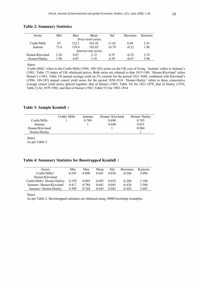
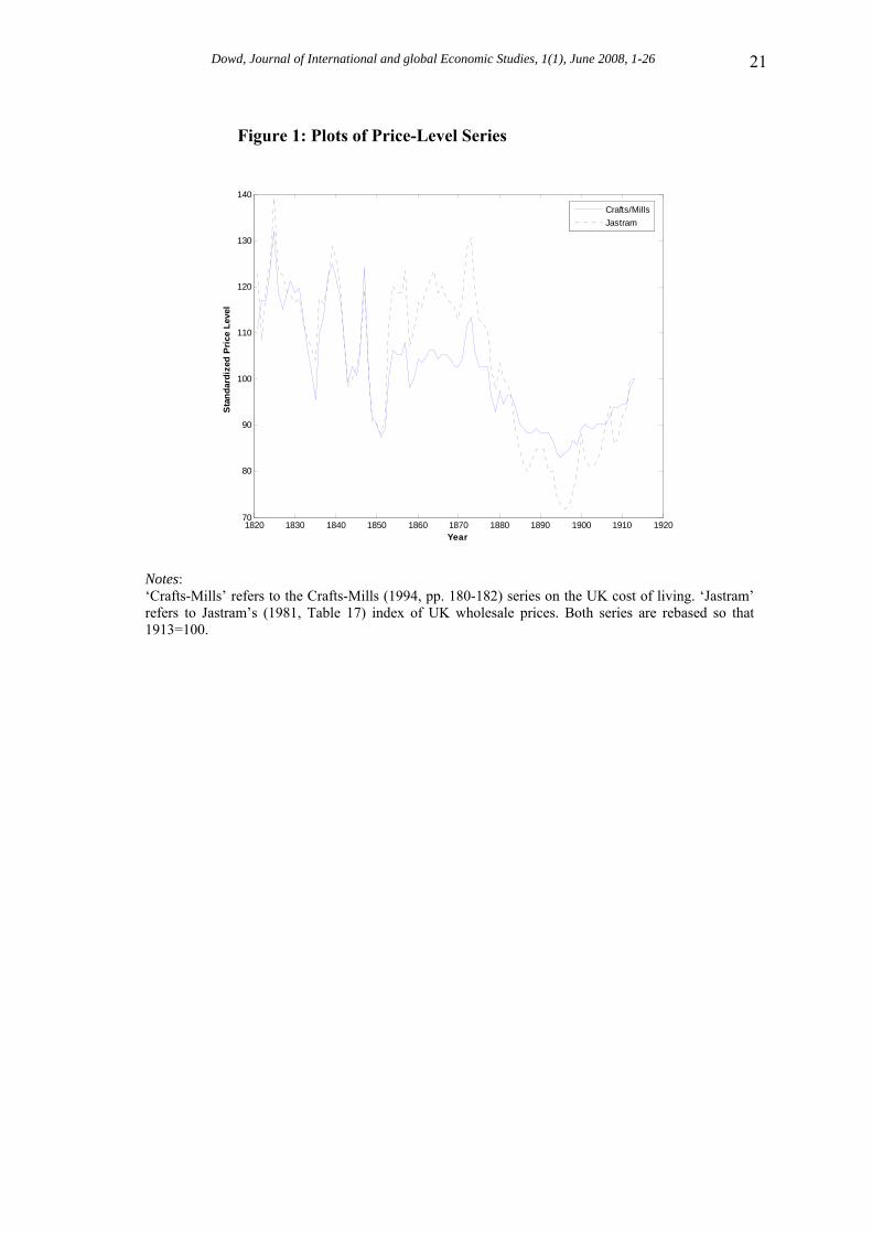
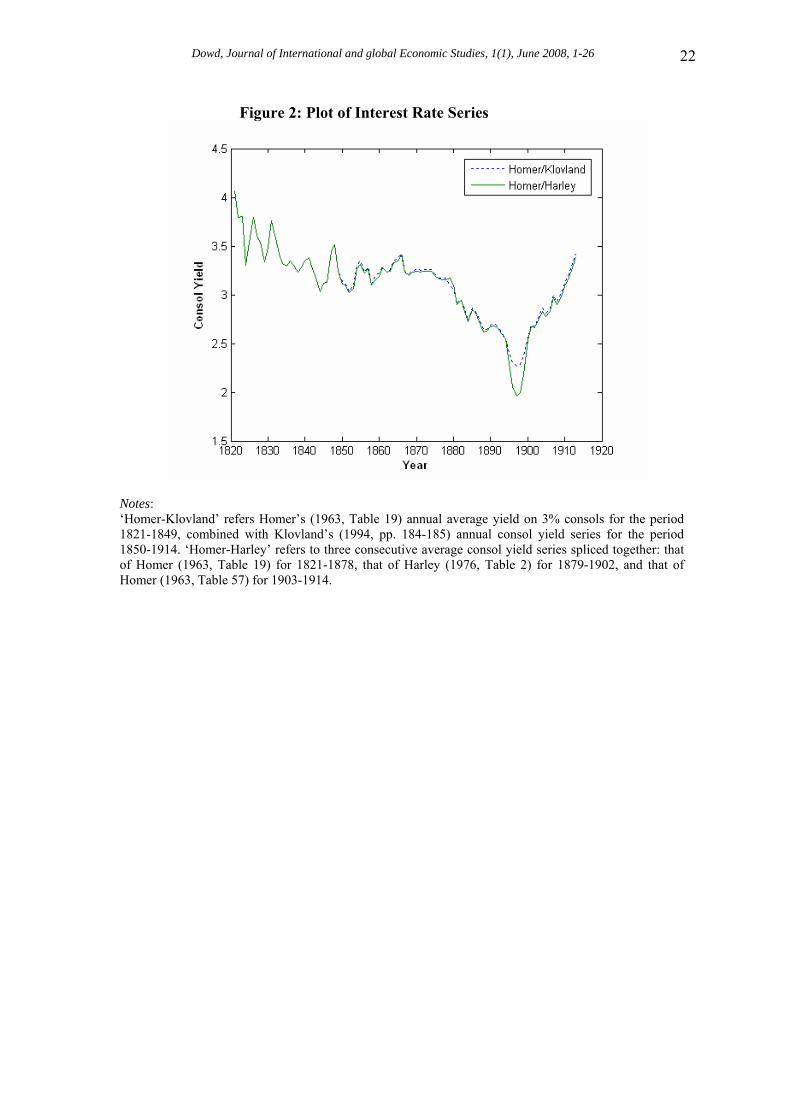
To illustrate the potential of copulas in macroeconomics, we now carry out a copula-based analysis of a well-known macroeconomic relationship, the Gibson paradox under gold standard. The Gibson paradox is of interest in its own right, but is also a convenient phenomenon for an illustrative copula analysis. This is because the Gibson paradox is an uncomplicated unconditional relationship between two easily observed variables.21 The focus of interest with the Gibson paradox is also very much on the dependence relationship rather the marginals, and its ‘core’ hypothesis – that of a positive correlation between interest rates and prices – is straightforward. 4.2. Data Our data set refers to the UK over its ‘golden’ gold standard period, 1821-1913. The price level was represented by one ‘traditional’ series (namely, Jastram’s (1981, Table 17) index of UK wholesale prices), and one new series that incorporates the impact of recent revisionist work on UK economic history (namely, the Crafts-Mills (1994, pp. 180-182) series on the UK cost of living). The interest rate was represented by (a) Homer’s (1963, Table 19) annual average yield on 3% consols for the period 1821-1849, combined with Klovland’s (1994, pp. 184-185) annual consol yield series for the period 1850-1914. As an alternative, the interest rate was also represented by (b) splicing three average consol yield series: that of Homer (1963, Table 19) for 1821-1878, that of Harley (1976, Table 2) for 1879-1902, and that of Homer (1963, Table 57) for 1903-1914. It is necessary to modify traditional UK consol series (e.g., Homer’s) for the later nineteenth century to take account of various pitfalls in earlier estimates of consol yields for that period (see, e.g., Klovland (1994, pp. 169-174)). We therefore use the Homer series as our base consol yield series, but for the sensitive period in question we use each of two alternative series suggested by Klovland and Harley that take account of (at least some of) the pitfalls in traditional series. 4.3. Preliminary Results Some plots of our price-level series given in Figure 1. These series move relatively close together, and show the features one would expect: an initial rise in the early 1820s; considerable volatility but an overall tendency to fall until the late 1840s; increases in the 1850s, the great depression that starts in the 1870s, and then the recovery starting in the 1890s; changes are also fairly volatile from year to year, and prices at the end of the period are not much different from what they were at the start of it. The corresponding plots for our interest rate series are given in Figure 2. The two interest rate series are very closely related. They show a broad but slight tendency for interest rates to fall until the 1870s, an accelerated fall after that, a big dip in the 1890s, and then a sharp recovery. Sample moments for our series are given in Table 2. These indicate that the price-level series exhibit less than normal kurtosis. However, the two interest rate series have (small) negative skews and exhibit greater than normal kurtosis. These results suggest that the two distributions might be non-normal and also different from each other.22


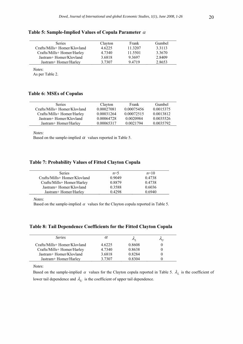
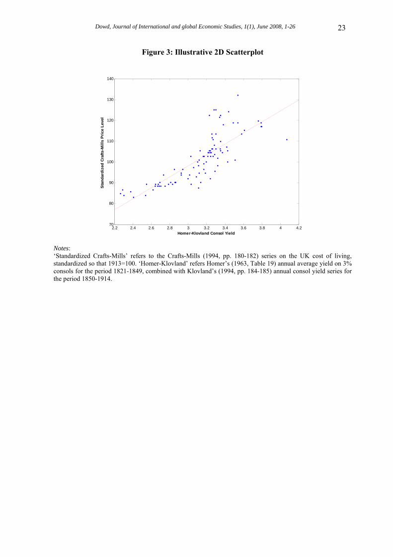
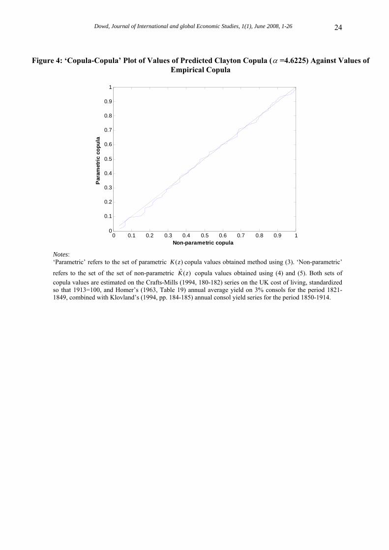
4.4. Correlation Results Figure 3 shows a 2D scatterplot for the illustrative combination of the Crafts-Mills price level and the Homer-Klovland consol yield. This plot strongly suggests that the two series have a positive association.23 Table 3 also shows the sample τ ’s between different combinations of price-level and interest-rate series. These are all positive (as predicted), and vary from a minimum of 0.648 (for that between the Jastram and Homer/Klovland series) to a maximum of 0.703 (for that between the Crafts/Mills and Homer/Harley series). To assess the strength of these correlations, Table 4 reports some bootstrapped correlation results based on 10,000 simulation trials. It is very interesting to see that every single bootstrapped estimate (i.e., for every simulation trial, across all pairs of price-level and interest-rate series) is positive: this finding suggests strong support for the Gibson paradox hypothesis of a positive (and significant) correlation between the price level and the interest rate over this period. 4.5. Copula Results We now look at our copula results, beginning with the values of α implied by the sample values of τ that were reported in Table 3. These implied values of α were obtained by plugging the sample τ values into (3) and solving for the corresponding values of α . These α values are given in Table 5. Inserting these values and the empirical distribution functions into the relevant copula equations (given in Table 1) then gives us our set of fitted Archimedean copulas. To determine which of these best fits the data, we estimate their MSEs relative to the empirical copula using the Genest-Rivest approach outlined in section 2.3. MSE results for the different copulas and each pair of price-level and interest-rate series are shown in Table 6. These results are very clear: in each case the Clayton copula gives us the minimum MSE, leading us to conclude that the Clayton copula always gives us the best fit. To assess the goodness of fit of our best fitted copula, Figure 4 presents a ‘copula-copula’ plot applied to the illustrative combination of the Crafts-Mills price-level and Homer-Klovland interest-rate series. If the copula fit is good, the fitted curve should be close to a 45 degree line, and we can see that this plot suggests a fairly close fit.24 To confirm this visual impression with formal tests, Table 7 shows the probability values for the hypothesis that the fitted copula provides an adequate fit. These are based on chi-squared goodness of fit tests predicated on 5 and 10 bins respectively. These p-value results indicate that the underlying hypothesis is acceptable for each combination of price-level and interest-rate series. The Clayton copula therefore provides a good fit in each case.


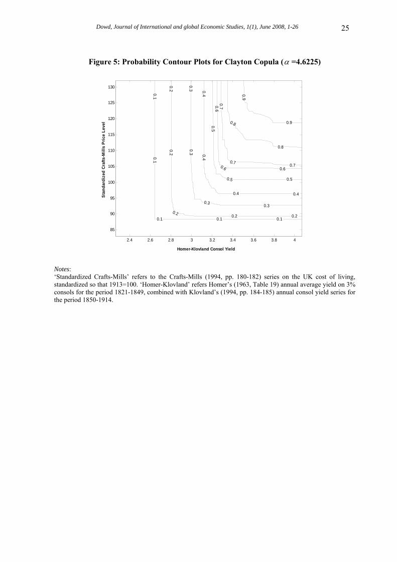
4.6. Investigating the Fitted Copula We now investigate the fitted copula, and Figure 5 provides the contour plot for the same combination of Crafts-Mills price level and Homer-Klovland consol yield. This plot exhibits the ‘close to L’ shape typical of series that have a strong positive correlation.25 The ‘L shape’ is particularly pronounced for low contour levels, but becomes somewhat less pronounced as the contour levels get bigger. To investigate the properties of the fitted copula, Table 8 shows the tail dependence coefficients of the fitted copula. The coefficients of upper tail dependence are necessarily 0, because the Clayton copula has no upper tail dependence. However, the Clayton does have lower tail dependence, and the results in the Table indicate that these are quite large, varying from just over 0.82 to just under 0.87. These results indicate that there is strong lower tail dependence, meaning that very low values of one variable are strongly associated with very low values of the other. This is a feature of the empirical Gibson paradox that has not (to my knowledge) been suggested before, and provides a strong hint that there is more to the Gibson paradox than just a positive correlation between interest and prices.26 It also of course indicates the ability of copula analysis to shed additional light on old phenomena.

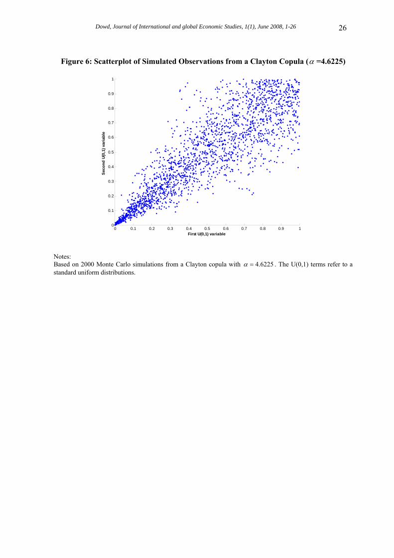
The tail dependence properties of the fitted copula also explain why the contour lines have such a strong ‘L’ shape for low contours, and a less pronounced ‘L’ shape for high contours. The tail dependence of the copula can also be seen in Figure 6. This provides a scatterplot of simulated ‘observations’ from the fitted copula. The plots reveals not only the strong positive correlation between the two random variables in their central mass region, but also shows that observations in the left hand tail (in the bottom left hand corner of the plot) have a strong association (i.e., are very clustered together) that is not present in the right-hand tail (in the top right of the plot, where they are much more dispersed). Figure 6 therefore illustrates both the positive correlation and the tail dependence of the copula in one plot. Indeed, we can go so far as to say that Figure 6 shows what the Gibson paradox ‘looks like’ when modelled using a copula. 5. Conclusions This paper has suggested that copulas provide a powerful and insightful tool for the analysis of macroeconomic relationships. It outlines the advantages of using copulas for investigating these relationships and suggests that copulas are much more flexible than traditional approaches. It also shows that copula analyses are able to provide new insight into multivariate relationships, and are especially good for flushing out the ways in which tail observations relate to each other. Our discussion focuses on Archimedean copulas because these are straightforward to apply, but the broad methodology applies to other copulas too (e.g., such as elliptical or Plackett copulas) and can be applied to more complicated relationships (such as those involving conditional dependence, common factors, etc.) or unobserved variables (e.g., the Fisher effect or the Philips curve).27 The basic principles also extend to relationships involving three or more random variables. In fact, copulas can be applied to any multivariate relationships.28


To demonstrate their potential, the paper provides as a worked example a copula-based analysis of the Gibson paradox under the gold standard using British data for the period 1821-1913. This example is a good one for illustrative purposes because the Gibson paradox is an uncomplicated relationship that has been well researched over the years, but is also interesting in its own right. Our analysis not only strongly confirms the ‘core’ Gibson paradox hypothesis – that interest rates and prices are positively correlated – but also sheds more light on the underlying phenomenon by providing evidence that the extremely low price-level and interest-rate observations have a strong correlation of their own, which extremely high observations do not. This appears to be a new finding and provides a nice illustration of the ability of copula analysis to shed new light on old problems. Endnotes * Kevin Dowd is professor of financial risk management at Nottingham University Business School. Address: Centre for Risk and Insurance Studies, Nottingham University Business School, Jubilee Campus, Nottingham NG8 1BB, UK; phone +44 115 846 6682, fax + 44 115 846 6667, email: [email protected]. This work was carried out under an ESRC research fellowship on ‘Risk Measurement in Financial Institutions’ (RES-000-27-0014) and the author thanks the ESRC for their financial support. He also thanks the editor, Yu Hsing, and Theo Panagiotidis for helpful inputs. The usual caveat applies. 1. A good introduction to copulas is provided by Embrechts et alia (2002), and the standard book-length references on copulas are Joe (1997), Nelson (1999) and Cherubini et alia (2004). More specific applications follow shortly in the text. 2. Methods very similar to copula ones have also been applied to extreme correlations in equity markets (e.g., Longin and Solnik (2001) and Poon et alia (2003)). 3. In fact, this paper is not the first to make this suggestion or to provide a macroeconomic application of copulas. The first paper to apply copulas to macroeconomics appears to be Granger et alia (2003). They used copula methods to examine common factors in conditional distributions for bivariate time series, and provided as an application of their method a copula-based analysis of the relationship between US income and consumption. 4. The best-known example of a conditional (and also time-dependent) copula model in finance is where a GARCH volatility model is fitted to the residuals from an equation that forecasts mean returns. The correlation is then fitted to the residuals conditional on the volatility forecasts. Some examples of such applications are provided by Chen et alia (2004) and Patton (2005). 5. Not only does the copula allow the modeller greater flexibility in the choice of marginals to be applied to each random variable, but it also increases the reliability of the estimation process by allowing for the marginals to be separately evaluated.


6. To give an example, if we assume multivariate normality, then we are implicitly assuming that the marginals are univariate normal, and this assumption will frequently be violated. However, with a copula, we can take the marginals as given, and are not forced to make strong assumptions about them. 7. We focus on Archimedean copulas because of their attractions explained in the text and also for reasons of space. However, there are other copulas that are also intuitive and tractable. These include elliptical (i.e., Gaussian and Student-t) copulas (see, e.g., Cherubini et alia (2004)), and Plackett copulas (see, e.g., Rockinger and Jondeau (2004)). 8. Their main limitation is that two of the standard Archimedeans, the Clayton and Gumbel, only allow positive dependence. However, this constraint is often not a binding one (e.g., as in the Gibson paradox application discussed later). Where it might be a problem, it can also be circumvented by redefining one of more of the random variables to ensure positive dependence. 9. In particular, it is defined over the range [-1,+], is invariant to monotone transformations, and takes the extreme values of 1 (or -1) iff Y=f(X) for some monotone increasing (decreasing) function (Genest and MacKay (1986, p. 282)). These attractive properties are not always shared by the more familiar Pearson correlation. 10. The key point here are that the sample estimator of τ has respectable properties and that the relationship between α and τ is one-to-one. Note, too, that estimating α from a sample estimate of τ also has the attraction that it allows us to estimate the copula without having to specify the marginals. Alternatively, we can also obtain estimates of α using ML or nonparametric methods, such as those discussed in note 20 below. 11. We can also select a copula using other criteria, such as entropy ones (as in Ané and Kharoubi (2003, p. 426)) or the Akaike Information Criterion. 12. Other possible tests include tests in the Kolgmorov-Smirnov and Anderson-Darling families, but these can be unreliable (Dowd (2005)). For more on these and other alternatives, see, e.g., Fermanian (2005) or Genest et alia (2005). 13. Chi-squared tests have been suggested by Dobrić and Schmid (2004), Savu and Trede (2004), and Dowd (2005), who all report results suggesting that they have respectable size and power properties when applied to Archimedean (and sometimes other) copulas. 14. For derivation, see, e.g., Cherubini et alia (2004, pp. 123, 127). 15. If we are working in a conditional modelling context we would also wish to carry out some formal time-series analysis (e.g., to determine the number of unit roots in the series, to determine if the series are cointegrated, etc.) to ensure that our later analysis has an adequate statistical underpinning. However, such analysis is not always necessary, especially in cases where the time-series properties of the data are not an issue (e.g., as in our later illustrative application to the Gibson paradox).


16. More generally, the key requirement here is that we choose a measure of association that is appropriate to the problem and copula at hand. In the case of the Archimedeans, this would be the Kendall τ correlation, in the case of ellipticals, it would be the Pearson correlation, and so forth. However, we cannot choose the association measure arbitrarily. For example, the Pearson correlation would obviously be inappropriate in cases where this correlation was not defined. 17. For more on bootstrap methods, see, e.g., Efron and Tibshirani (1993) or Davison and Hinckley (1997). 18. As noted in footnote 10, this step is not always necessary if we have Archimedean copulas and use the Genest-Rivest method to estimate α from a sample estimate of τ . However, it is generally good practice to examine the marginals, and in some situations this will be mandatory. 19. It also has the advantage that it avoids distracting the reader’s attention with additional issues related to the estimation of the marginals, which are not really of much concern here. 20. The ML methods include exact ML, which applies to marginals and copulas simultaneously), the IFM (inference for the margins) method (Joe and Xu (1996), which is a two-step approximation to exact ML, and canonical ML, which focuses on ML estimation of the copula itself. The non-parametric methods include empirical copulas (Deheuvels (1979)) and kernel copulas (e.g., Scaillet (2000)). For more on estimation methods, see, e.g., Cheribuni et alia (2004, chapter 5). 21. Keynes famously described the Gibson paradox as “one of the most completely established empirical facts in the whole field of quantitative economics” (1930, p. 198). Many others endorsed this view, including Friedman and Schwartz (1982), who reported strong evidence for it in the period before the First World War. There have been critics of the Gibson paradox – such as Benjamin and Kochin (1984, pp. 601-602), who concluded that the correlation between the price level and the rate of interest was essentially spurious and due to the influence of wartime financial factors – but the overwhelming majority of studies have produced results supportive of the paradox (e.g., Barsky and Summers (1988), Mills (1990), Dowd and Sampson (1993), and Dowd and Harrison (2000)). 22. Although there is no strict requirement that we do so, we could also investigate the series’ time-series properties. If we did so, we would find that we could reasonably accept the hypothesis that all series have a single unit root, and that the relevant pairs of price-level and interest-rate series are cointegrated. However, the detailed results are not reported here. 23. The scatterplots for other combinations of price-level and interest-rate series are not different in any particularly noteworthy way. The similarity of the scatterplots is also consistent with the sample Kendall τ correlations in Table 3 that show that the different price-level series tend to be highly positively correlated with each, and that the two interest rate series also have a high positive correlation. 24. The comparable plots involving the other pairs of series are similar to Figure 4.


25. Low values of τ produce contour curves that are much smoother, but asτ gets bigger, the curves tend to a pronounced ‘L’ shape. Thus, a pronounced ‘L’ shape is indicative of high degrees of positive association. 26. This finding corresponds neatly to the increasingly well-established finding that financial markets also exhibit lower tail dependence but not upper tail dependence, i.e., that correlations tend to rise in strong bear markets, but not in strong bull markets. Evidence for this finding in equity markets is provided in Solnik and Longin (2001), Ané and Kharoubi (2003), Poon et alia (2003), Patton (2004) and Rockinger and Jondeau (2004), and comparable evidence for FX markets is provided by Breymann et alia (2003) and Patton (2005). 27. In these circumstances, we would also have to deal with such issues as whether to specify a fixed dependence structure (as has usually been done in copula studies to date) or whether to allow a dynamic copula (e.g., as in Rockinger and Jondeau (2004) or Goorbergh et alia (2005)). 28. Another interesting extension is suggested by Poon et alia (2003): they suggest that in cases where the focus of interest is exclusively with the dependence structure, then ‘complications’ arising from the behavior of the marginals can be minimized by transforming the marginals so that they obey a common distribution. References Ané, T., and C. Kharoubi. 2003. “Dependence Structure and Risk Measure,” Journal of Business, 76, 411-438. Ang, A. and J. Chen. 2002. “Asymmetric Correlations of Equity Portfolios,” Journal of Financial Economics, 63, 443-494. Barsky, R. B. and L. H. Summers. 1988. “Gibson’s Paradox and the Gold Standard,” Journal of Political Economy, 96, 528-550. Benjamin, D. K. and Kochin, L. A. 1984. “War, Prices and Interest Rates: A Martial Solution to Gibson’s Paradox,” In M. D Bordo and A. J Schwartz (Eds), A Retrospective on the Classical Gold Standard 1821-1931, 587-604. Chicago: University of Chicago Press. Breymann, W., A. Dias, and P. Embrechts. 2003. “Dependence Structures for Multivariate High-Frequency Data in Finance,” Quantitative Finance, 3, 1-14. Chen, X., Y. Fan and A. J. Patton. 2004. “Simple Tests for Models of Dependence between Multiple Financial Time Series, with Applications to US Equity Returns and Exchange Rates,” Working paper, New York University, Vanderbilt University, and London School of Economics. Cherubini, U. and E. Luciano. 2001. “Value-at-Risk Trade-Off and Capital Allocation with Copulas,” Economic Notes, 30, 235-256.


Cherubini, U. and E. Luciano. 2002. “Bivariate Option Pricing with Copulas.” Applied Mathematical Finance, 8, 69-85. Cherubini, U., E. Luciano, and W. Vecchiato. 2004. Copula Methods in Finance. Chichester: John Wiley. Clayton, D. G. 1978. “A Model for Association in Bivariate Life Tables and its Application in Epidemiological Studies of Familial Tendency in Chronic Disease Incidence,” Biometrika, 65, 141-151. Crafts, N. F. R. and T. C. Mills 1994. “Trends in Real Wages in Britain, 1750-1913,” Explorations in Economic History, 31, 176-194. Davison, A. C. and D. V. Hinkley. 1997. Bootstrap Methods and their Applications. Cambridge: Cambridge University Press. Deheuvels, P. 1979. “La function de dépendence empirique et ses propriétés. Un test non paramétriquen d’indépendence,” Acad. Roy. Belg. Bull C1. Sci., 65, 274-292. Dobrić, J., and F. Schmid. 2004. “Testing Goodness of Fit for Parametric Families of Copulas – Application toFfinancial Data,” Working paper, University of Cologne. Dowd, K. 2005. “A Framework to Evaluate Fitted Copulas,” Working paper. Nottingham University Business School. Dowd, K. and B. Harrison. 2000. “The Gibson Paradox and the Gold Standard: Evidence from the United Kingdom, 1821-1913.” Applied Economics Letters, 7, 711-713. Dowd, K. and A. A. Sampson. 1993. “The Gold Standard, Gibson’s Paradox and the Gold Stock,” Journal of Macroeconomics, 15, 653-659. Efron, B. and R. J. Tibshirani. 1993. An Introduction to the Bootstrap. New York and London: Chapman and Hall, 1993. Embrechts, P., A. J. McNeil, and D. Straumann. 2002. “Correlation and Dependence in Risk Management: Properties and Pitfalls,” pp. 176-223 in M. Dempster (Ed.) Risk Management: Value at Risk and Beyond. Cambridge: Cambridge University Press. Fermanian, J.-D. 2005. “Goodness-of-Fit Tests for Copulas,” Journal of Multivariate Analysis, 95, 119-152. Frank, M. J. 1979. “On the Simultaneous Associativity of F(x,y) and x+y-F(x,y).” Aequationes Math., 19, 194-226. Frees, E. W., and E. Valdez. 1998. “Understanding Relationships Using Copulas,” North American Actuarial Journal, 2, 1-25.


Friedman, M., and A. J. Schwartz. 1982. Monetary Trends in the United States and the United Kingdom. Chicago: University of Chicago Press. Genest, C. and J. MacKay. 1986 “The Joy of Copulas: Bivariate Distributions with Uniform Marginals,” American Statistician, 40, 280-283. Genest, C. and L.-P. Rivest. 1993. “Statistical Inference Procedures for Bivariate Archimedean Copulas,” Journal of the American Statistical Association, 88, 1034-1043. Genest, C., J.-F. Quessy, and B. Rémillard. 2005, “Goodness-of-Fit Procedures for Copula Models Based on the Probability Integral Transformation,” Scandinavian Journal of Statistics 32: 1-30. Goorbergh, R. W. J. van den, C. Genest, and B. J. M. Werker. 2005. “Bivariate Option Pricing Using Dynamic Copula Models,” Insurance: Mathematics and Economics, 37, 101-114. Granger, C. W. J., T. Teräsvirta, and A. J. Patton. 2003. “Common Factors in Conditional Distributions for Bivariate Time Series,” mimeo. University of California, San Diego; Stockholm School of Economics; and London School of Economics. Gumbel, E. J. 1960. “Bivariate Exponential Distributions,” Journal of the American Statistical Association, 55, 698-707. Harley, C. K. 1976 “Goschen’s Conversion of the National Debt and the Yield on Consols,” Economic History Review, 29, 101-106. Homer, S. 1963. A History of Interest Rates. New Brunswick, NJ: Rutgers University Press. Jastram, R. W. 1981. Silver: The Restless Metal. New York: John Wiley and Sons. Joe, H. 1997. Multivariate Models and Dependence Concepts. London: Chapman and Hall. Joe, H. and J. J. Xu.1996. “The Estimation Method of Inference Functions for Margins for Multivariate Models,” University of British Columbia Department of Statistics Technical Report 166. Keynes, J. M. 1930. A Treatise on Money, Volume Two, London: Macmillan. Kiley, M. T. 2003. “Why is Inflation Low When Productivity Growth is High?” Economic Inquiry, 41, 392-406. Klovland, J. T. 1994. “Pitfalls in the Estimation of the Yield on British Consols, 1850-1914,” Journal of Economic History, 54, 164-187.

Dowd, Journal of International and global Economic Studies, 1(1), June 2008, 1-26

17

Li, D. 2000. “On Default Correlation: A Copula Function Approach,” Journal of Fixed Income, 9, 43-55. Longin, F. M. and B. Solnik. 2001 “Extreme Correlation of International Equity Markets,” Journal of Finance, 56, 649-676. Mills, T. C. 1990. “A Note on the Gibson Paradox during the Gold Standard,” Explorations in Economic History, 27, 277-286. Nelson, R. B. 1999. An Introduction to Copulas. New York: Springer. Patton, A. J. 2004. “On the Importance of Skewness and Asymmetric Dependence in Stock Returns for Asset Allocation,” Journal of Financial Econometrics, 2, 130-168. Patton, A. J. 2005. “Modelling Time-Varying Exchange Rate Dependence,” International Economic Review, forthcoming. Poon, S.-H., M. Rockinger, and J. Tawn. 2003. “Extreme Value Dependence in Financial Markets: Diagnostics, Models, and Financial Implications,” Review of Financial Studies, 17, 581-610. Rockinger, M. and E. Jondeau. 2004 “Conditional Dependence of Financial Series: The Copula-GARCH Model,” Universite Paris XII, working paper 02-04. Rodriguez, J. C. 2003. “Measuring Financial Contagion: A Copula Approach,” mimeo. EURANDOM, Eindhoven. Savu, C. and M. Trede. 2004. “Goodness-of-Fit Tests for Parametric Families of Archimedean Copulas,” Working paper, University of Münster. Scaillet, O. 2000. “Nonparametric Estimation of Copulas for Time Series,” working paper, Université Catholique de Louvain. Sklar, A. 1959. “Fonctions de Repartition à n dimensions et leur merges.” Publ. Inst. Stat. Univ. Paris, 8, 229-231.


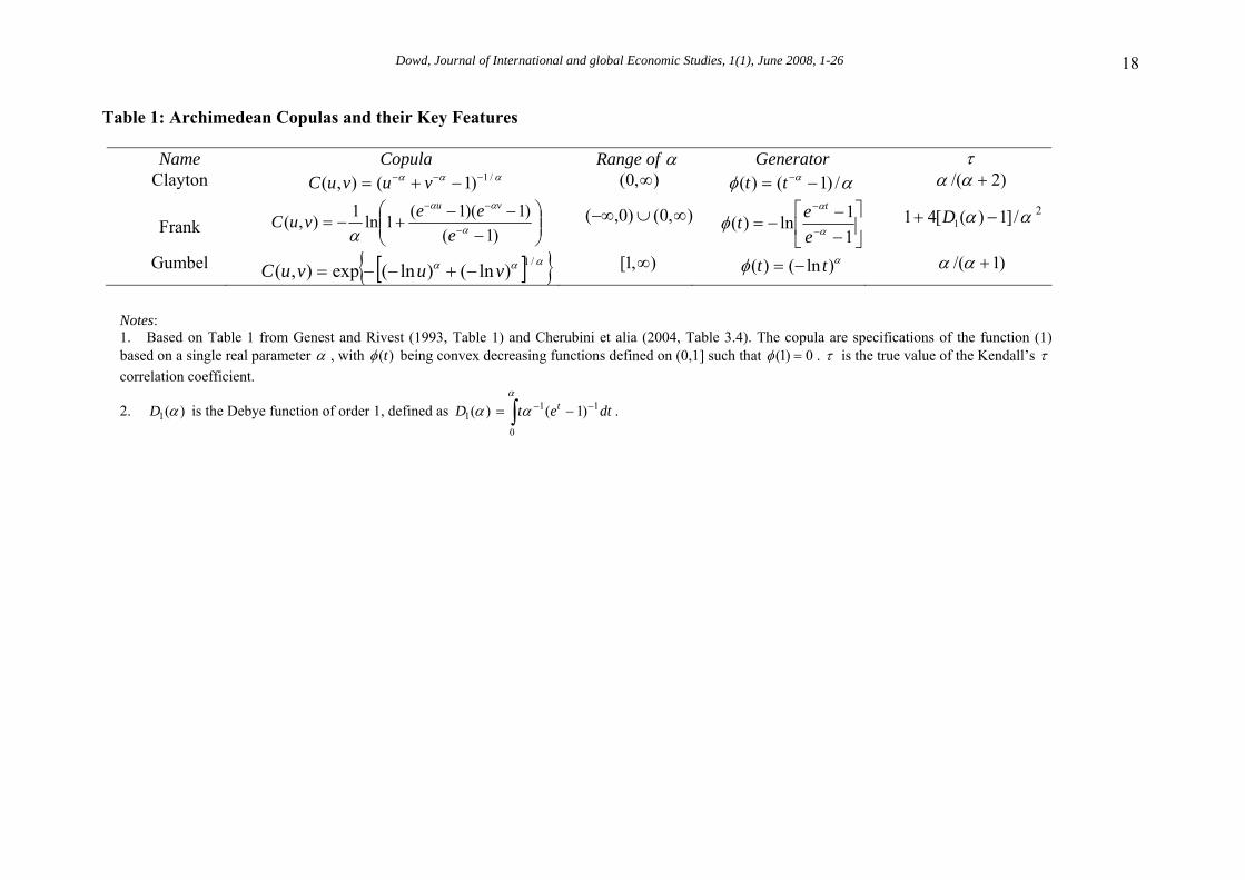
Table 1: Archimedean Copulas and their Key Features

Name Copula Range of α Generator τ Clayton ααα /1)1(),( −−− −+= vuvuC ),0( ∞ αφ α /)1()( −= −tt )2/( +αα

Frank ⎟⎟

⎠

⎞⎜⎜⎝

⎛−

−−+−= −

−−

)1()1)(1(1ln1),( α

αα

α eeevuC

vu

),0()0,( ∞∪−∞⎥⎦

⎤⎢⎣

⎡−−

−= −

−

11ln)( α

α

φeet

tαα /]1)([41 1 −+ D 2

Gumbel [ ]{ }ααα /1)ln()ln(exp),( vuvuC −+−−= ),1[ ∞ αφ )ln()( tt −= )1/( +αα

Notes: 1. Based on Table 1 from Genest and Rivest (1993, Table 1) and Cherubini et alia (2004, Table 3.4). The copula are specifications of the function (1) based on a single real parameter α , with ( )tφ being convex decreasing functions defined on (0,1] such that 0)1( =φ . τ is the true value of the Kendall’s τ correlation coefficient.

2. )(1 αD is the Debye function of order 1, defined as )(1 αD = ∫ −− −α

α0

11 )1( dtet t .


Table 2: Summary Statistics

Series Min Max Mean Std Skewness Kurtosis Price-level series

Crafts/Mills 83 132.1 101.42 11.62 0.48 2.41 Jastram 71.8 139.4 103.83 16.79 -0.22 1.86

Interest-rate series Homer/Klovland 2.26 4.07 3.12 0.35 -0.32 3.19

Homer/Harley 1.96 4.07 3.10 0.39 -0.67 3.98

Notes: ‘Crafts-Mills’ refers to the Crafts-Mills (1994, 180-182) series on the UK cost of living. ‘Jastram’ refers to Jastram’s (1981, Table 17) index of UK wholesale prices. Both series are rebased so that 1913=100. ‘Homer-Klovland’ refers Homer’s (1963, Table 19) annual average yield on 3% consols for the period 1821-1849, combined with Klovland’s (1994, 184-185) annual consol yield series for the period 1850-1914. ‘Homer-Harley’ refers to three consecutive average consol yield series spliced together: that of Homer (1963, Table 19) for 1821-1878, that of Harley (1976, Table 2) for 1879-1902, and that of Homer (1963, Table 57) for 1903-1914.

Table 3: Sample Kendall τ

Crafts/ Mills Jastram Homer/ Klovland Homer/ Harley

Crafts/Mills 1 0.789 0.698 0.703 Jastram 1 0.648 0.651

Homer/Klovland 1 0.964 Homer/Harley 1

Notes: As per Table 2.

Table 4: Summary Statistics for Boostrapped Kendall τ

Series Min Max Mean Std Skewness Kurtosis Crafts/Mills+

Homer/Klovland 0.543 0.800 0.691 0.036 -0.266 3.096

Crafts/Mills+ Homer/Harley 0.559 0.803 0.695 0.035 -0.286 3.100 Jastram+ Homer/Klovland 0.417 0.784 0.641 0.045 -0.426 3.380

Jastram+ Homer/Harley 0.399 0.768 0.643 0.045 -0.485 3.603

Notes: As per Table 2. Bootstrapped estimates are obtained using 10000 bootstrap resamples.


Table 5: Sample-Implied Values of Copula Parameter α

Series Clayton Frank Gumbel Crafts/Mills+ Homer/Klovland 4.6225 11.3207 3.3113

Crafts/Mills+ Homer/Harley 4.7340 11.5501 3.3670 Jastram+ Homer/Klovland 3.6818 9.3697 2.8409

Jastram+ Homer/Harley 3.7307 9.4719 2.8653

Notes: As per Table 2.

Table 6: MSEs of Copulas

Series Clayton Frank Gumbel Crafts/Mills+ Homer/Klovland 0.00027081 0.00075456 0.0015375

Crafts/Mills+ Homer/Harley 0.00031264 0.00072515 0.0013812 Jastram+ Homer/Klovland 0.00064728 0.0020984 0.0035526

Jastram+ Homer/Harley 0.00065317 0.0021794 0.0035792 Notes: Based on the sample-implied α values reported in Table 5.

Table 7: Probability Values of Fitted Clayton Copula

Series n=5 n=10

Crafts/Mills+ Homer/Klovland 0.9049 0.4738 Crafts/Mills+ Homer/Harley 0.8879 0.4738 Jastram+ Homer/Klovland 0.3588 0.6036

Jastram+ Homer/Harley 0.4298 0.6940

Notes: Based on the sample-implied α values for the Clayton copula reported in Table 5.

Table 8: Tail Dependence Coefficients for the Fitted Clayton Copula

Series α Lλ Uλ

Crafts/Mills+ Homer/Klovland 4.6225 0.8608 0 Crafts/Mills+ Homer/Harley 4.7340 0.8638 0 Jastram+ Homer/Klovland 3.6818 0.8284 0

Jastram+ Homer/Harley 3.7307 0.8304 0

Notes: Based on the sample-implied α values for the Clayton copula reported in Table 5. Lλ is the coefficient of

lower tail dependence and Uλ is the coefficient of upper tail dependence.


Figure 1: Plots of Price-Level Series

1820 1830 1840 1850 1860 1870 1880 1890 1900 1910 192070

80

90

100

110

120

130

140

Year

Stan

dard

ized

Pric

e Le

vel

Crafts/MillsJastram

Notes: ‘Crafts-Mills’ refers to the Crafts-Mills (1994, pp. 180-182) series on the UK cost of living. ‘Jastram’ refers to Jastram’s (1981, Table 17) index of UK wholesale prices. Both series are rebased so that 1913=100.


Figure 2: Plot of Interest Rate Series

Notes: ‘Homer-Klovland’ refers Homer’s (1963, Table 19) annual average yield on 3% consols for the period 1821-1849, combined with Klovland’s (1994, pp. 184-185) annual consol yield series for the period 1850-1914. ‘Homer-Harley’ refers to three consecutive average consol yield series spliced together: that of Homer (1963, Table 19) for 1821-1878, that of Harley (1976, Table 2) for 1879-1902, and that of Homer (1963, Table 57) for 1903-1914.


Figure 3: Illustrative 2D Scatterplot

2.2 2.4 2.6 2.8 3 3.2 3.4 3.6 3.8 4 4.270

80

90

100

110

120

130

140

Homer-Klovland Consol Yield

Stan

dard

ized

Cra

fts-M

ills

Pric

e Le

vel

Notes: ‘Standardized Crafts-Mills’ refers to the Crafts-Mills (1994, pp. 180-182) series on the UK cost of living, standardized so that 1913=100. ‘Homer-Klovland’ refers Homer’s (1963, Table 19) annual average yield on 3% consols for the period 1821-1849, combined with Klovland’s (1994, pp. 184-185) annual consol yield series for the period 1850-1914.


Figure 4: ‘Copula-Copula’ Plot of Values of Predicted Clayton Copula (α =4.6225) Against Values of

Empirical Copula

0 0.1 0.2 0.3 0.4 0.5 0.6 0.7 0.8 0.9 10

0.1

0.2

0.3

0.4

0.5

0.6

0.7

0.8

0.9

1

Non-parametric copula

Par

amet

ric c

opul

a

Notes: ‘Parametric’ refers to the set of parametric copula values obtained method using (3). ‘Non-parametric’

refers to the set of the set of non-parametric copula values obtained using (4) and (5). Both sets of copula values are estimated on the Crafts-Mills (1994, 180-182) series on the UK cost of living, standardized so that 1913=100, and Homer’s (1963, Table 19) annual average yield on 3% consols for the period 1821-1849, combined with Klovland’s (1994, pp. 184-185) annual consol yield series for the period 1850-1914.

)(zK

(K )z


Figure 5: Probability Contour Plots for Clayton Copula (α =4.6225)

0.10.1

0.1 0.1 0.10.2

0.2

0.2 0.2 0.2

0.30.3

0.3 0.3

0.40.4

0.4 0.4

0.50.5 0.5

0.6

0.6 0.60.7

0.7 0.7

0.8

0.80.9

0.9

Homer-Klovland Consol Yield

Sta

ndar

dize

d Cr

afts

-Mill

s P

rice

Leve

l

2.4 2.6 2.8 3 3.2 3.4 3.6 3.8 4

85

90

95

100

105

110

115

120

125

130

Notes: ‘Standardized Crafts-Mills’ refers to the Crafts-Mills (1994, pp. 180-182) series on the UK cost of living, standardized so that 1913=100. ‘Homer-Klovland’ refers Homer’s (1963, Table 19) annual average yield on 3% consols for the period 1821-1849, combined with Klovland’s (1994, pp. 184-185) annual consol yield series for the period 1850-1914.

Dowd, Journal of International and global Economic Studies, 1(1), June 2008, 1-26

26

Figure 6: Scatterplot of Simulated Observations from a Clayton Copula (α =4.6225)

0 0.1 0.2 0.3 0.4 0.5 0.6 0.7 0.8 0.9 10

0.1

0.2

0.3

0.4

0.5

0.6

0.7

0.8

0.9

1

First U(0,1) variable

Sec

ond

U(0,

1) v

aria

ble

Notes: Based on 2000 Monte Carlo simulations from a Clayton copula with 6225.4=α . The U(0,1) terms refer to a standard uniform distributions.

Download - Copulas in Macroeconomics - Southeastern Louisiana …...Copulas in Macroeconomics . Kevin Dowd* Centre for Risk and Insurance Studies . Nottingham University Business School . Abstract

Top Related