Download - Approaches to real world two-dimensional cutting problems

Applications

Approaches to real world two-dimensional cutting problems

Enrico Malaguti a,n, Rosa Medina Durán b, Paolo Toth a

a DEI, University of Bologna, Viale Risorgimento 2, 40136 Bologna, Italyb Departamento de Ingeniería Industrial, Facultad de Ingeniería, Universidad de Concepción, Chile

a r t i c l e i n f o

Article history:Received 9 October 2012Accepted 29 August 2013

Keywords:2-Dimensional cutting stockColumn generationHeuristics

a b s t r a c t

We consider a real world generalization of the 2-Dimensional Guillotine Cutting Stock Problem arising inthe wooden board cutting industry. A set of rectangular items has to be cut from rectangular stock boards,available in multiple formats. In addition to the classical objective of trim loss minimization, the problemalso asks for the maximization of the cutting equipment productivity, which can be obtained by cuttingidentical boards in parallel. We present several heuristic algorithms for the problem, explicitly consideringthe optimization of both objectives. The proposed methods, including fast heuristic algorithms, IntegerLinear Programming models and a truncated Branch and Price algorithm, have increasing complexity andrequire increasing computational effort. Extensive computational experiments on a set of realistic instancesfrom the industry show that high productivity of the cutting equipment can be obtained with a minimalincrease in the total area of used boards. The experiments also show that the proposed algorithms performextremely well when compared with four commercial software tools available for the solution of theproblem.

& 2013 Elsevier Ltd. All rights reserved.

1. Introduction

Given a set of rectangular items and infinitely many identicalrectangular stock boards, the Two-Dimensional Cutting Stock Pro-blem (2DCSP) asks for cutting all the items by using the minimumnumber of boards or, equivalently, by minimizing the area of theused boards. In this paper we consider a generalization of theproblem, which models with adequate detail real world situationsarising in the wooden board cutting industry. The problem is knownto be NP-hard since it generalizes the Bin Packing Problem [18].

In wooden board cutting, a set of rectangular items has to be cutfrom rectangular stock boards, which are usually available inmultiple formats. Some items may be rotated, while others mayhave a compulsory orientation, which is determined by the woodgrain. The main objective, as in classical cutting stock problems, isthe stock usage (or equivalently, the trim loss) minimization,which is evaluated in terms of area (or cost) of used boards. Asecond objective is the maximization of machine productivity, acommon objective in many industrial settings. Machine produc-tivity is usually maximized by reducing the number of setups in aproduction process (see Allahverdi et al. [1]), as it is done, e.g.,when scheduling the sequence of operations on computer numer-ical control systems (see Zamiri Marvizadeh and Choobineh [24]),

or by defining optimal sequences of operations when the setuptimes are sequence-dependent (see, e.g., Pan and Ruiz [19]). Inwooden board cutting, instead, productivity can be improved byprocessing several items at the same time, as explained in thefollowing.

A few approaches are available for multi-objective optimizationproblems like the one we consider (see e.g., [16,4]), and the waythe two objectives are jointly optimized in practice depends on thespecific industrial setting. However, in the commercial softwaretools used in the wooden board cutting industry, it is usual tooptimize as an objective function a weighted combination of usedstock area and machine productivity.

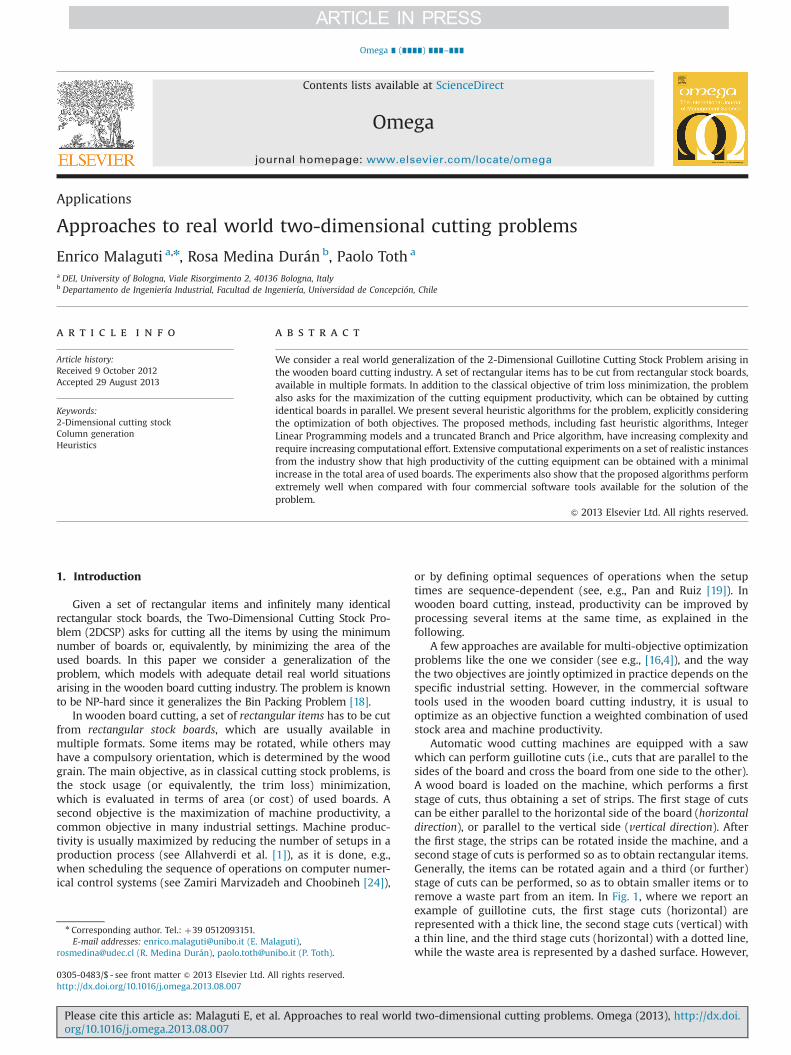
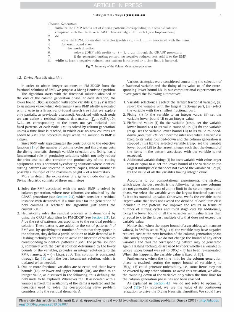
Automatic wood cutting machines are equipped with a sawwhich can perform guillotine cuts (i.e., cuts that are parallel to thesides of the board and cross the board from one side to the other).A wood board is loaded on the machine, which performs a firststage of cuts, thus obtaining a set of strips. The first stage of cutscan be either parallel to the horizontal side of the board (horizontaldirection), or parallel to the vertical side (vertical direction). Afterthe first stage, the strips can be rotated inside the machine, and asecond stage of cuts is performed so as to obtain rectangular items.Generally, the items can be rotated again and a third (or further)stage of cuts can be performed, so as to obtain smaller items or toremove a waste part from an item. In Fig. 1, where we report anexample of guillotine cuts, the first stage cuts (horizontal) arerepresented with a thick line, the second stage cuts (vertical) witha thin line, and the third stage cuts (horizontal) with a dotted line,while the waste area is represented by a dashed surface. However,

Contents lists available at ScienceDirect

journal homepage: www.elsevier.com/locate/omega

Omega

0305-0483/$ - see front matter & 2013 Elsevier Ltd. All rights reserved.http://dx.doi.org/10.1016/j.omega.2013.08.007

n Corresponding author. Tel.: þ39 0512093151.E-mail addresses: [email protected] (E. Malaguti),

[email protected] (R. Medina Durán), [email protected] (P. Toth).

Please cite this article as: Malaguti E, et al. Approaches to real world two-dimensional cutting problems. Omega (2013), http://dx.doi.org/10.1016/j.omega.2013.08.007i

Omega ∎ (∎∎∎∎) ∎∎∎–∎∎∎

www.sciencedirect.com/science/journal/03050483

www.elsevier.com/locate/omega

http://dx.doi.org/10.1016/j.omega.2013.08.007



mailto:[email protected]








while the first and second stages can be automatically managed bythe machine, the third (and higher) stage cuts usually require themanual intervention of an operator. Thus, if on one hand cuts ofthird (and higher) stage increase the opportunities of the stockusage minimization, on the other hand their use reduces themachine productivity. We only consider cuts up to the third stage.

A peculiarity of wood cutting consists of the possibility ofstacking in a pile several identical boards, say h, which can be cutwith a single cutting cycle, thus obtaining h copies of each itemcontained in a single board. This possibility leads to a dramaticproductivity increase. Clearly, the geometry of the cuts to beperformed, i.e., the so-called cutting pattern, must be the samefor all the stacked boards, and thus the parallel cut of stackedboards limits the opportunities of stock usage minimization. Givena pattern to be repeated r times and a maximum number κ ofboards for a board pile, we have to perform c¼ dr=κ⌉ cuttingcycles.

As anticipated, we are considering a multi-objective optimizationproblem, for which it is not possible to define a unique approach,valid for any industrial setting. The two objectives of stock usageminimization and machine productivity are partially in contrast, andin theory it would be interesting, although impractical, to enumerateall the Pareto-efficient solutions to the problem. In practice commer-cial software tools produce one solution, and have some flexibility ongiving more importance to trim loss minimization or productivity.Thus, in this paper we use a scalarization technique, and evaluate asolution to the cutting problem according to a generic weightedobjective function, including three different terms: the area of usedboards, the number of cutting cycles and the number of third stagecuts, where the last two terms are strongly correlated with machineproductivity.

Other approaches for multi-objective optimization problemsinclude the ε-constraints method, where one objective is mini-mized, and the remaining objectives are constrained to be lessthan or equal to given target values; the goal programming, whichcan be seen as the search for a solution satisfying specific goalvalues of the objectives, or the solution closest to the specifiedgoals if none exists satisfying the goal values; the lexicographicmethod, where the objective functions are arranged in order ofimportance, then the minimizers of the first objective function arefound; secondly, the minimizers of the second objective functionare searched for, and so on, until all the objective functions havebeen optimized on successively smaller sets. For a deeper analysisof multi-objective optimization we refer the reader to the survey[16] and the book [4] and the references therein.

Although commercial software tools are designed to implicitlytake into account the minimization of cutting cycles and thirdstage cuts, quite often these two objectives, and their relativeimportance with respect to the minimization of the area of usedboards, are not stated explicitly, and are obtained as a side-productof the optimization. In our research, we show instead thatexplicitly considering cutting cycles and third stage cuts allowone to obtain solutions which are much more efficient withrespect to these two dimensions, at a very small cost in terms ofthe area of used boards.

More formally, we consider a real world 2DCSP with thefollowing additional features:

� the items must be obtained from stock boards through at mostthree-staged guillotine cuts;

� some items have a fixed orientation with respect to the boardsides, while other items may be orthogonally rotated;

� board rotation is allowed (i.e., the first stage can be eitherhorizontal or vertical with respect to the board side);

� boards of multiple formats are available;� up to κ boards can be stacked in a pile and cut with a single

cutting cycle;� the area of used stock A, the number of cutting cycles C, and the

number of third stage cuts Z have to be globally minimized,according to the weighted objective function:

min w1Aþw2Cþw3Z ð1Þwhere w1, w2 and w3 are given non-negative weights.

Hence, the input data defining an instance of the problem are: alist of m rectangular item classes, each item class i with dimensionsðli;wiÞ, a demand di and an attribute specifying if the item can beorthogonally rotated, and a list of b rectangular board classes, eachboard class k with dimensions ðLk;WkÞ and available in an infinitenumber of copies. In the following, li and Lk will be denoted as lengthof an item class i and of a board class k, respectively; wi and Wk willbe denoted as width of an item class i and a board class k,respectively. The maximum number κ of stack boards in a pile andthe weights w1, w2 and w3 of the objective function conclude theinput data. For each item class i, the number of produced items canexceed the corresponding demand di (the overproduced items areconsidered as waste). Following the typology introduced by Wäscheret al. [23] and by disregarding the component of the problem relatedto productivity, the problem can be classified as a Two-DimensionalMultiple Stock Size Cutting Stock Problem. Other real world general-izations of the 2DCSP, characterized by dimension, planning situa-tion, goal, restrictions and solution approach, are described byDyckhoff et al. [6].

According to the literature on cutting stock problems, the realworld problem we consider combines a generalization of the2DCSP with a variant of the Pattern Minimization Problem, whichwas mainly addressed in the one-dimensional case (see, e.g.,[13,22,21,3]). Note that pattern minimization goes in the directionof productivity but it is not precisely the same as minimization ofthe cutting cycles and of the third stage cuts.

The 2DCSP was introduced by Gilmore and Gomory [10–12],who also considered the k-staged version of the problem and alsoconsidered boards of different dimensions. Riehme et al. [20]considered the two-staged version of the problem in the casewhere boards of different dimensions are available and the itemdemands differ in a large range. Cintra et al. [5] considered several2DCSPs with guillotine cuts and their variants in which orthogonalrotations are allowed and boards of different dimensions areavailable. They presented dynamic programming algorithms forthe Two-Dimensional Knapsack Problem (2DKP), which are thenused to generate patterns in approaches for the 2DCSP based oncolumn generation. Given a set of rectangular items with asso-ciated positive profits and one rectangular bin, the 2DKP is to cutthe subset of items of maximum profit which can fit into the bin.Recently, Furini et al. [9] proposed a column-generation basedheuristic for the 2DCSP, where orthogonal rotations are allowedand boards of different dimensions are available, which improveson previously known results from the literature. Exact models forthe same problem (without rotation) were proposed and compu-tationally compared by Furini and Malaguti [8]. The problemaddressed in [9,8] does not consider the possibility of stacking

Fig. 1. Guillotine cuts.

E. Malaguti et al. / Omega ∎ (∎∎∎∎) ∎∎∎–∎∎∎2






several boards in a pile and of third-stage cuts, and thus does notconsider the optimization of cycles. In addition, the problemaddressed in [9,8] only considers two-stage cuts plus trimming,i.e., third stage cuts are only allowed for removing a waste area.A survey on several Two-Dimensional Packing Problems can befound in Lodi et al. [15].

The literature on the One-Dimensional Cutting Stock Problemwith Pattern Minimization considers the case of identical boards.An early heuristic was proposed by Haessler [13], where the cost ofusing a pattern is added as an additional cost term to the objectivefunction, and new patterns are iteratively added to the currentsolution by taking into account their trim loss and the possibilityof multiple usage. A metaheuristic approach to the problem wasproposed by Umetani et al. [21], where the number of differentcutting patterns is an input parameter and different solutions aregenerated by binary search. Belov and Scheithauer [3] proposed asequential heuristic for the combined minimization of the trimloss and of the number of different cutting patterns. Concerningexact approaches, Vanderbeck [22] presented an ILP (IntegerLinear Programming) formulation and a Branch-and-Cut-and-Price algorithm for minimizing the number of different patterns,once the maximum number of used boards is fixed as a constraint.

The main contribution of this paper is to propose severalalgorithms for a real world 2DCSP explicitly considering theoptimization of the three objectives mentioned in Eq. (1). Sincethe problem considers the machine productivity maximization(PM) in a 2DCSP setting, we denote it as PM-2DCSP. The proposedalgorithms have increasing complexity and require increasingcomputational effort. Extensive computational experiments showthat high productivity of the cutting equipment can be obtainedwith a minimal increase in the total area of used boards.

More in detail, in Section 2 we describe three fast heuristicalgorithms for the PM-2DCSP, and a procedure for reducing thenumber of cutting cycles. The aim of these algorithms is to obtaingood quality solutions in short computing time. In Section 3 wepresent a straightforward integration of the three algorithmsthrough the solution of an optimization model which is able toproduce improved solutions. In Section 4 the best performingalgorithm among the previously described ones is embedded intoan overall method, based on a truncated Branch-and-Price frame-work. The computing time of this algorithm is limited to 10 min, inorder to have a tool of practical utility, and, for the same reason, inthis algorithm we do not make use of any commercial software.The paper is concluded by a set of computational experiments(Section 5), where the proposed algorithms are tested and com-pared with 4 commercial software tools on a set of realisticinstances derived from real world problems from the wood cuttingindustry.

2. Heuristic algorithms

In this section we describe three heuristic algorithms whichsolve the PM-2DCSP by generating patterns composed by strips.A strip parallel to the board length (resp. width) is said ahorizontal (resp. vertical) strip. Given a horizontal strip, the itemsare obtained by cutting the strip with vertical guillotine cuts. Thestrip width is defined by the widest contained item (or by thelongest item if the item is rotated), and the strip length is thelength of the board that contains the strip. If the items in the striphave different widths or are stacked within the strip, a trimmingcut (third stage) is used to obtain the desired widths. The itemscan be stacked (i.e., placed one over the other in a strip) when theyhave the same length and the strip width is larger than the sum ofthe widths of the items. Similar definitions can be stated for the“vertical” strips by swapping the “lengths” and the “widths”.

At each step of the algorithms described in the followingsections, we denote the set of available items as the set of itemswhich still have to be included into a cutting pattern. During thestrip generation, the algorithms ask for the solution of severalBounded Knapsack Problems (BKPs). Given a set of items each onehaving an associated positive weight, profit and number of copies,and a knapsack (bin) of fixed capacity, the BKP is to select thesubset of items of maximum profit whose cumulative weight doesnot exceed the knapsack capacity, and such that no more than thenumber of available copies of each item are selected (see [18,14]).Since the BKPs are solved several times and many solutions arediscarded, we do not look for the optimal solution of each BKP, butwe heuristically solve the problem in a greedy way by ordering theitems according to a specified rule and considering the items forinsertion in this order.

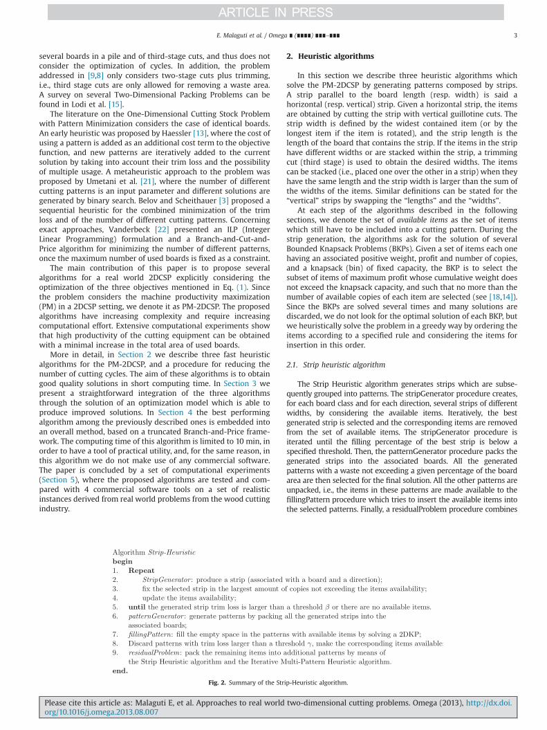
2.1. Strip heuristic algorithm

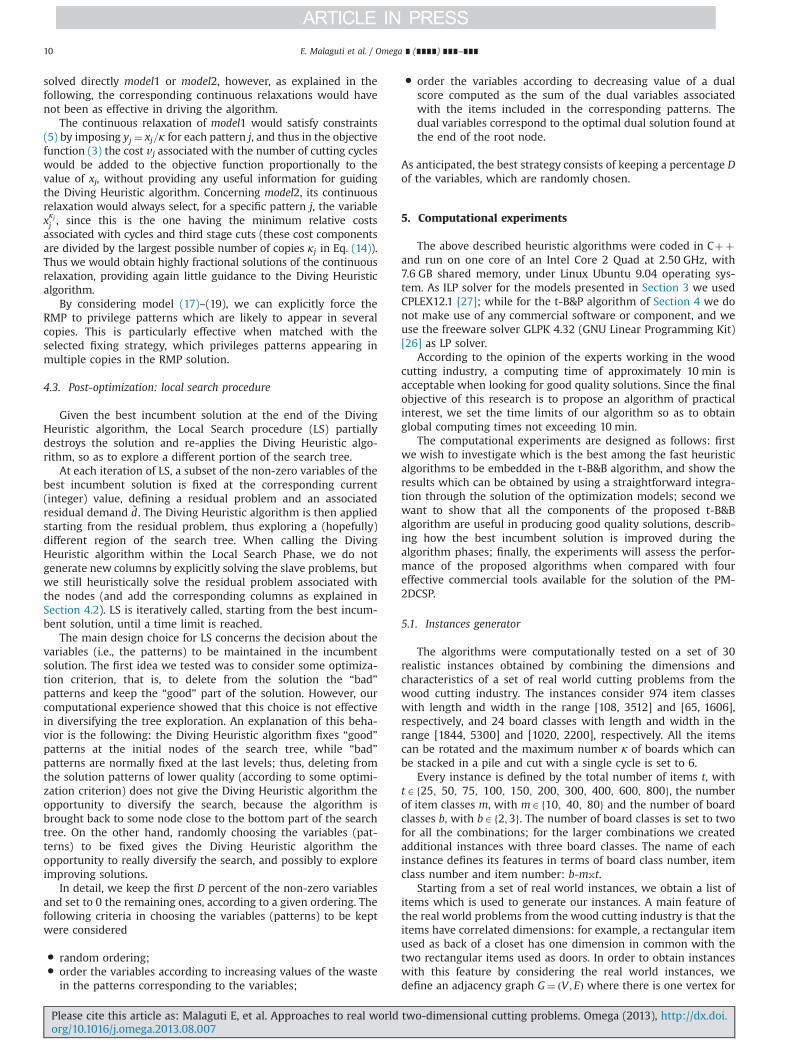
The Strip Heuristic algorithm generates strips which are subse-quently grouped into patterns. The stripGenerator procedure creates,for each board class and for each direction, several strips of differentwidths, by considering the available items. Iteratively, the bestgenerated strip is selected and the corresponding items are removedfrom the set of available items. The stripGenerator procedure isiterated until the filling percentage of the best strip is below aspecified threshold. Then, the patternGenerator procedure packs thegenerated strips into the associated boards. All the generatedpatterns with a waste not exceeding a given percentage of the boardarea are then selected for the final solution. All the other patterns areunpacked, i.e., the items in these patterns are made available to thefillingPattern procedure which tries to insert the available items intothe selected patterns. Finally, a residualProblem procedure combines

Fig. 2. Summary of the Strip-Heuristic algorithm.

E. Malaguti et al. / Omega ∎ (∎∎∎∎) ∎∎∎–∎∎∎ 3






the remaining items into patterns. The details of these procedures aregiven in the following. A summary of the Strip Heuristic algorithm isgiven in Fig. 2.

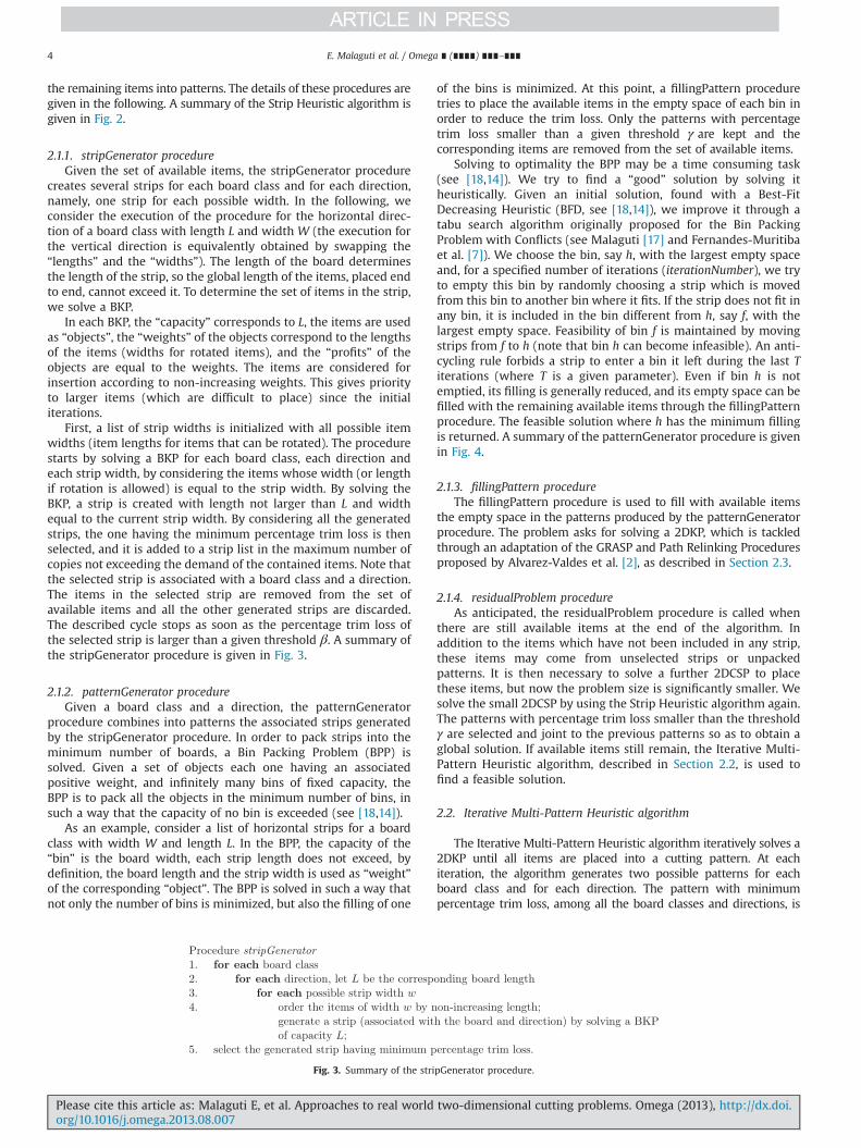
2.1.1. stripGenerator procedureGiven the set of available items, the stripGenerator procedure

creates several strips for each board class and for each direction,namely, one strip for each possible width. In the following, weconsider the execution of the procedure for the horizontal direc-tion of a board class with length L and width W (the execution forthe vertical direction is equivalently obtained by swapping the“lengths” and the “widths”). The length of the board determinesthe length of the strip, so the global length of the items, placed endto end, cannot exceed it. To determine the set of items in the strip,we solve a BKP.

In each BKP, the “capacity” corresponds to L, the items are usedas “objects”, the “weights” of the objects correspond to the lengthsof the items (widths for rotated items), and the “profits” of theobjects are equal to the weights. The items are considered forinsertion according to non-increasing weights. This gives priorityto larger items (which are difficult to place) since the initialiterations.

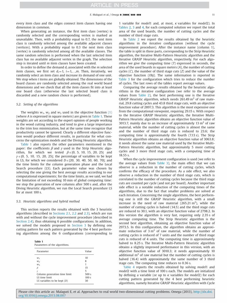
First, a list of strip widths is initialized with all possible itemwidths (item lengths for items that can be rotated). The procedurestarts by solving a BKP for each board class, each direction andeach strip width, by considering the items whose width (or lengthif rotation is allowed) is equal to the strip width. By solving theBKP, a strip is created with length not larger than L and widthequal to the current strip width. By considering all the generatedstrips, the one having the minimum percentage trim loss is thenselected, and it is added to a strip list in the maximum number ofcopies not exceeding the demand of the contained items. Note thatthe selected strip is associated with a board class and a direction.The items in the selected strip are removed from the set ofavailable items and all the other generated strips are discarded.The described cycle stops as soon as the percentage trim loss ofthe selected strip is larger than a given threshold β. A summary ofthe stripGenerator procedure is given in Fig. 3.

2.1.2. patternGenerator procedureGiven a board class and a direction, the patternGenerator

procedure combines into patterns the associated strips generatedby the stripGenerator procedure. In order to pack strips into theminimum number of boards, a Bin Packing Problem (BPP) issolved. Given a set of objects each one having an associatedpositive weight, and infinitely many bins of fixed capacity, theBPP is to pack all the objects in the minimum number of bins, insuch a way that the capacity of no bin is exceeded (see [18,14]).

As an example, consider a list of horizontal strips for a boardclass with width W and length L. In the BPP, the capacity of the“bin” is the board width, each strip length does not exceed, bydefinition, the board length and the strip width is used as “weight”of the corresponding “object”. The BPP is solved in such a way thatnot only the number of bins is minimized, but also the filling of one

of the bins is minimized. At this point, a fillingPattern proceduretries to place the available items in the empty space of each bin inorder to reduce the trim loss. Only the patterns with percentagetrim loss smaller than a given threshold γ are kept and thecorresponding items are removed from the set of available items.

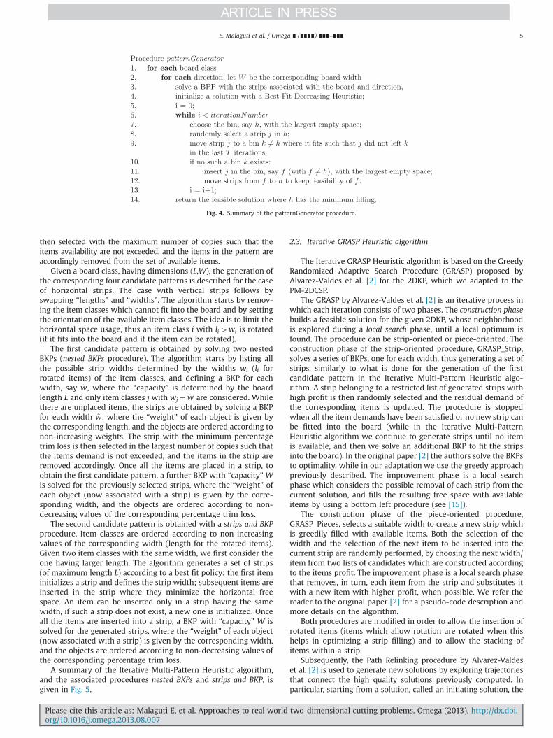
Solving to optimality the BPP may be a time consuming task(see [18,14]). We try to find a “good” solution by solving itheuristically. Given an initial solution, found with a Best-FitDecreasing Heuristic (BFD, see [18,14]), we improve it through atabu search algorithm originally proposed for the Bin PackingProblem with Conflicts (see Malaguti [17] and Fernandes-Muritibaet al. [7]). We choose the bin, say h, with the largest empty spaceand, for a specified number of iterations (iterationNumber), we tryto empty this bin by randomly choosing a strip which is movedfrom this bin to another bin where it fits. If the strip does not fit inany bin, it is included in the bin different from h, say f, with thelargest empty space. Feasibility of bin f is maintained by movingstrips from f to h (note that bin h can become infeasible). An anti-cycling rule forbids a strip to enter a bin it left during the last Titerations (where T is a given parameter). Even if bin h is notemptied, its filling is generally reduced, and its empty space can befilled with the remaining available items through the fillingPatternprocedure. The feasible solution where h has the minimum fillingis returned. A summary of the patternGenerator procedure is givenin Fig. 4.

2.1.3. fillingPattern procedureThe fillingPattern procedure is used to fill with available items

the empty space in the patterns produced by the patternGeneratorprocedure. The problem asks for solving a 2DKP, which is tackledthrough an adaptation of the GRASP and Path Relinking Proceduresproposed by Alvarez-Valdes et al. [2], as described in Section 2.3.

2.1.4. residualProblem procedureAs anticipated, the residualProblem procedure is called when

there are still available items at the end of the algorithm. Inaddition to the items which have not been included in any strip,these items may come from unselected strips or unpackedpatterns. It is then necessary to solve a further 2DCSP to placethese items, but now the problem size is significantly smaller. Wesolve the small 2DCSP by using the Strip Heuristic algorithm again.The patterns with percentage trim loss smaller than the thresholdγ are selected and joint to the previous patterns so as to obtain aglobal solution. If available items still remain, the Iterative Multi-Pattern Heuristic algorithm, described in Section 2.2, is used tofind a feasible solution.

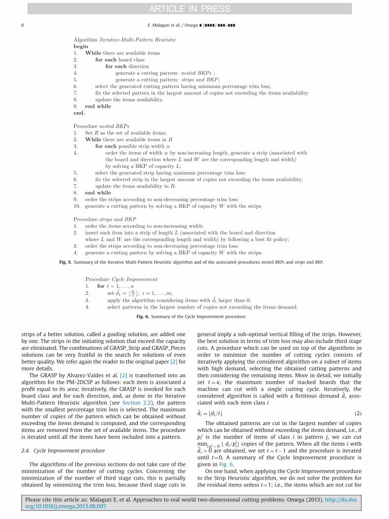
2.2. Iterative Multi-Pattern Heuristic algorithm

The Iterative Multi-Pattern Heuristic algorithm iteratively solves a2DKP until all items are placed into a cutting pattern. At eachiteration, the algorithm generates two possible patterns for eachboard class and for each direction. The pattern with minimumpercentage trim loss, among all the board classes and directions, is

Fig. 3. Summary of the stripGenerator procedure.







then selected with the maximum number of copies such that theitems availability are not exceeded, and the items in the pattern areaccordingly removed from the set of available items.

Given a board class, having dimensions (L,W), the generation ofthe corresponding four candidate patterns is described for the caseof horizontal strips. The case with vertical strips follows byswapping “lengths” and “widths”. The algorithm starts by remov-ing the item classes which cannot fit into the board and by settingthe orientation of the available item classes. The idea is to limit thehorizontal space usage, thus an item class i with li4wi is rotated(if it fits into the board and if the item can be rotated).

The first candidate pattern is obtained by solving two nestedBKPs (nested BKPs procedure). The algorithm starts by listing allthe possible strip widths determined by the widths wi (li forrotated items) of the item classes, and defining a BKP for eachwidth, say ~w , where the “capacity” is determined by the boardlength L and only item classes j with wj ¼ ~w are considered. Whilethere are unplaced items, the strips are obtained by solving a BKPfor each width ~w , where the “weight” of each object is given bythe corresponding length, and the objects are ordered according tonon-increasing weights. The strip with the minimum percentagetrim loss is then selected in the largest number of copies such thatthe items demand is not exceeded, and the items in the strip areremoved accordingly. Once all the items are placed in a strip, toobtain the first candidate pattern, a further BKP with “capacity” Wis solved for the previously selected strips, where the “weight” ofeach object (now associated with a strip) is given by the corre-sponding width, and the objects are ordered according to non-decreasing values of the corresponding percentage trim loss.

The second candidate pattern is obtained with a strips and BKPprocedure. Item classes are ordered according to non increasingvalues of the corresponding width (length for the rotated items).Given two item classes with the same width, we first consider theone having larger length. The algorithm generates a set of strips(of maximum length L) according to a best fit policy: the first iteminitializes a strip and defines the strip width; subsequent items areinserted in the strip where they minimize the horizontal freespace. An item can be inserted only in a strip having the samewidth, if such a strip does not exist, a new one is initialized. Onceall the items are inserted into a strip, a BKP with “capacity” W issolved for the generated strips, where the “weight” of each object(now associated with a strip) is given by the corresponding width,and the objects are ordered according to non-decreasing values ofthe corresponding percentage trim loss.

A summary of the Iterative Multi-Pattern Heuristic algorithm,and the associated procedures nested BKPs and strips and BKP, isgiven in Fig. 5.

2.3. Iterative GRASP Heuristic algorithm

The Iterative GRASP Heuristic algorithm is based on the GreedyRandomized Adaptive Search Procedure (GRASP) proposed byAlvarez-Valdes et al. [2] for the 2DKP, which we adapted to thePM-2DCSP.

The GRASP by Alvarez-Valdes et al. [2] is an iterative process inwhich each iteration consists of two phases. The construction phasebuilds a feasible solution for the given 2DKP, whose neighborhoodis explored during a local search phase, until a local optimum isfound. The procedure can be strip-oriented or piece-oriented. Theconstruction phase of the strip-oriented procedure, GRASP_Strip,solves a series of BKPs, one for each width, thus generating a set ofstrips, similarly to what is done for the generation of the firstcandidate pattern in the Iterative Multi-Pattern Heuristic algo-rithm. A strip belonging to a restricted list of generated strips withhigh profit is then randomly selected and the residual demand ofthe corresponding items is updated. The procedure is stoppedwhen all the item demands have been satisfied or no new strip canbe fitted into the board (while in the Iterative Multi-PatternHeuristic algorithm we continue to generate strips until no itemis available, and then we solve an additional BKP to fit the stripsinto the board). In the original paper [2] the authors solve the BKPsto optimality, while in our adaptation we use the greedy approachpreviously described. The improvement phase is a local searchphase which considers the possible removal of each strip from thecurrent solution, and fills the resulting free space with availableitems by using a bottom left procedure (see [15]).

The construction phase of the piece-oriented procedure,GRASP_Pieces, selects a suitable width to create a new strip whichis greedily filled with available items. Both the selection of thewidth and the selection of the next item to be inserted into thecurrent strip are randomly performed, by choosing the next width/item from two lists of candidates which are constructed accordingto the items profit. The improvement phase is a local search phasethat removes, in turn, each item from the strip and substitutes itwith a new item with higher profit, when possible. We refer thereader to the original paper [2] for a pseudo-code description andmore details on the algorithm.

Both procedures are modified in order to allow the insertion ofrotated items (items which allow rotation are rotated when thishelps in optimizing a strip filling) and to allow the stacking ofitems within a strip.

Subsequently, the Path Relinking procedure by Alvarez-Valdeset al. [2] is used to generate new solutions by exploring trajectoriesthat connect the high quality solutions previously computed. Inparticular, starting from a solution, called an initiating solution, the

Fig. 4. Summary of the patternGenerator procedure.







strips of a better solution, called a guiding solution, are added oneby one. The strips in the initiating solution that exceed the capacityare eliminated. The combinations of GRASP_Strip and GRASP_Piecessolutions can be very fruitful in the search for solutions of evenbetter quality. We refer again the reader to the original paper [2] formore details.

The GRASP by Alvarez-Valdes et al. [2] is transformed into analgorithm for the PM-2DCSP as follows: each item is associated aprofit equal to its area; iteratively, the GRASP is invoked for eachboard class and for each direction, and, as done in the IterativeMulti-Pattern Heuristic algorithm (see Section 2.2), the patternwith the smallest percentage trim loss is selected. The maximumnumber of copies of the pattern which can be obtained withoutexceeding the items demand is computed, and the correspondingitems are removed from the set of available items. The procedureis iterated until all the items have been included into a pattern.

2.4. Cycle Improvement procedure

The algorithms of the previous sections do not take care of theminimization of the number of cutting cycles. Concerning theminimization of the number of third stage cuts, this is partiallyobtained by minimizing the trim loss, because third stage cuts in

general imply a sub-optimal vertical filling of the strips. However,the best solution in terms of trim loss may also include third stagecuts. A procedure which can be used on top of the algorithms inorder to minimize the number of cutting cycles consists ofiteratively applying the considered algorithm on a subset of itemswith high demand, selecting the obtained cutting patterns andthen considering the remaining items. More in detail, we initiallyset t ¼ κ, the maximum number of stacked boards that themachine can cut with a single cutting cycle. Iteratively, theconsidered algorithm is called with a fictitious demand ~di asso-ciated with each item class i

~di ¼ ⌊di=t⌋ ð2ÞThe obtained patterns are cut in the largest number of copies

which can be obtained without exceeding the items demand, i.e., ifpi

j is the number of items of class i in pattern j, we can cutmini:pji 40 ⌊ di=p

ji⌋ copies of the pattern. When all the items i with

~di40 are obtained, we set t ¼ t�1 and the procedure is iterateduntil t¼0. A summary of the Cycle Improvement procedure isgiven in Fig. 6.

On one hand, when applying the Cycle Improvement procedureto the Strip Heuristic algorithm, we do not solve the problem forthe residual items unless t¼1; i.e., the items which are not cut for

Fig. 6. Summary of the Cycle Improvement procedure.

Fig. 5. Summary of the Iterative Multi-Pattern Heuristic algorithm and of the associated procedures nested BKPs and strips and BKP.







a specified value of t are made available at the following iteration,when a smaller value of t is considered.

On the other hand, applying the Cycle Improvement proceduredirectly on top of the Iterative Multi-Pattern Heuristic algorithmand the Iterative GRASP Heuristic algorithm may lead to disap-pointing results, since patterns containing only few items may beobtained in t copies. Thus, for each value of t we compute the ratiobetween the sum of the areas of the items having ~di40 and thearea of the smallest board, and we skip the current value of t if thisratio is smaller than 1.

3. ILP models for the PM-2DCSP

This section proposes two alternative ILP formulations for thePM-2DCSP. Both formulations extend the well-known approach tothe Cutting Stock Problem proposed by Gilmore and Gomory [10]for the one-dimensional case, and require an exponential numberof variables. In particular, the two formulations differ in the waythe number of cutting cycles and the associated cost are expressed.Each feasible pattern j ðj¼ 1;…;nÞ is associated with a vectorPj ¼ ½p1j …pij…pmj �AZm where pj

i represents the number of items ofitem class i ði¼ 1;…;mÞ that are in pattern j. Given a pattern j, thenumber of third-stage cuts Zj, the associated board Bj and the set ofitem classes included in the pattern Ij (with Ij ¼ fi : pij40g) can becomputed.

The first formulation, denoted as model1, is a classical CuttingStock model where, for each feasible cutting pattern j, there is aninteger variable xj denoting the number of times the pattern isselected in the solution. In addition, integer variables yj denote thenumber of cutting cycles which are needed to obtain xj patterns,namely, yj ¼ dxj=κ⌉. model1 reads

min ∑n

j ¼ 1ðf jxjþvjyjÞ ð3Þ

s:t: ∑n

j ¼ 1pijxjZdi i¼ 1;…;m ð4Þ

yjZxjκ j¼ 1;…;n ð5Þ

xjAZþ ; yjAZþ j¼ 1;…;n ð6ÞThe cost fj associated with each variable xj (j¼1,…,n) depends

on the area of the corresponding board Bj; by calling Aj the area ofthe board class used for pattern j, fj is defined as

f j ¼w1Aj ð7Þthe cost vj associated with each variable yj is defined as

vj ¼w2þw3Zj ð8Þwhere w1, w2 and w3 are the weights given to the area, number ofcycles and number of third stage cuts in the objective function (1),respectively.

In order to strengthen the Linear Programming (LP) relaxationof the model, we add the following constraints that impose aminimum number of variables to cover each item class:

∑j:iA Ij

xjZminj:iA Ij

dipij

& ’( )i¼ 1;…;m ð9Þ

In the second formulation, denoted as model2, we do not use yvariables to count the number of cutting cycles, instead, for eachfeasible cutting pattern j ðj¼ 1;…;nÞ we have κj copies of the integervariable xj of the previous model, denoted as xj

t ðt ¼ 1;…; κjÞ. κjdenotes the maximum number of copies of pattern j in a cycle:κj ¼minfκ;maxiA Ij f⌈di=pij⌉gg. Thus, a variable xj

t taking a valuelarger than 0 means that txtj copies of pattern j are in the solution

and are obtained through xjt cutting cycles. A similar duplication of

the variables was used by Vanderbeck [22] for modeling theminimization of the number of cutting patterns in a cutting stockproblem. The xj

t variables are defined as binary for ðt ¼ 1;…; κj�1Þand integer for t ¼ κj. model2 reads

min ∑n

j ¼ 1∑κ

t ¼ 1Ctj x

tj ð10Þ

s:t: ∑n

j ¼ 1∑κ

t ¼ 1tpijx

tj Zdi i¼ 1;…;m ð11Þ

xtj Af0;1g j¼ 1;…;n t ¼ 1;…; κj�1 ð12Þ

xκjj AZþ j¼ 1;…;n ð13Þ

Each variable xjt (j¼1,…,n; t ¼ 1;…; κj) has a cost Cj

t thatincludes the costs associated with the board area Aj, the cuttingcycles and the number of third stage cuts Zj. Cjt is defined as

Ctj ¼ tw1Ajþw2þw3Zj ð14Þ

In this way any integer number of copies of pattern j can beobtained and the corresponding cost is imposed, e.g., if κ ¼ κj ¼ 6,to denote 14 copies of pattern j a min cost integer solution isx2j ¼ 1, x6j ¼ 2, corresponding to 3 cutting cycles, 3Zj third stagecuts and a global area equal to 14Aj. In order to strengthen the LPrelaxation of the model, we add the following constraints thatimpose a minimum number of variables to cover each item class.

∑j:iA Ij

∑κ

t ¼ 1xtj Zmin

j:iA Ij

dipij

& ’( )i¼ 1;…;m ð15Þ

For the binaries variables, we add the following constraints toavoid symmetric solutions:

∑κj �1

t ¼ 1xtj r1 j¼ 1;…;n ð16Þ

The optimal solution of both models requires column generationtechniques to manage the exponential number of variables involvedin the corresponding LP relaxations, and the computational effortwould make the method unpractical for solving real world pro-blems. However good heuristic solutions can be obtained byconsidering a subset of the variables xj (or xj

t), as explained in thefollowing.

3.1. A hybrid method

The solutions obtained from the heuristic algorithms describedin Section 2 can be combined and improved through model1 ormodel2. The idea is to solve the models by considering the subsetof xj (or xjt) variables corresponding to the set of feasible solutionsobtained by the heuristic algorithms. In detail, in the hybridmethod we propose, we apply the 3 heuristic algorithms, withand without the cycle improvement procedure for each instance,thus obtaining 6 feasible and (possibly) different solutions. Eachsolution determines a set of cutting patterns, which can be used todefine the corresponding xj (or xj

t) variables. In the following(see Section 5), we will consider the subset of cutting patternsgenerated by the best performing heuristic algorithms. The modelsare then solved by using a general purpose ILP solver, with a suitedtime limit. The best among the solutions found by the selectedheuristic algorithms and the models is given as final solution.

4. An algorithm for the PM-2DCSP

In the previous section we introduced three fast heuristicalgorithms and discussed a straightforward integration through







the solution of an ILP model. In this section we go a step further,and propose a truncated Branch-and-Price algorithm for the PM-2DCSP, denoted as t-B&P, which uses as subroutines some of theprocedures previously presented, and tackles an approximatedversion of the models discussed in Section 3. The algorithm wepropose is based on a column generation approach embeddedwithin a diving heuristic so as to obtain integer solutions. Thealgorithm is concluded by a Local Search procedure. The algorithmoptimizes a weighted combination of trim loss and productivity ofthe cutting equipment, according to the weighted objective func-tion (1), which is considered every time a new solution isproduced and compared with the best incumbent one.

The algorithm starts by computing an initial feasible solutionthrough the Iterative GRASP Heuristic algorithm with CycleImprovement. The cutting patterns corresponding to this startingsolution are used to initialize the set P which corresponds to thevariables of a cutting-stock ILP model. Then, new patterns areheuristically generated according to dual information from thecontinuous relaxation of the model, until no new columns havingnegative reduced cost can be generated or a time limit is reached.In the following we will denote the solution obtained at the end ofthis procedure as root node solution.

If the root node solution is not integer, integrality is obtainedwith a diving procedure. The diving procedure iteratively bounds aselected variable and solves the continuous relaxation of thecorresponding ILP model, possibly enlarging the set P with newcutting patterns having negative reduced cost, until an integersolution is obtained. Each step of the diving procedure corre-sponds to the exploration of a node in an associated Branch-and-Bound tree which is explored according to a depth-first strategy.The exploration terminates when the first integer solution isobtained (note that backtracking steps executed in order toexhaustively explore the search tree would require an unaccep-table computing effort for practical applications).

As an additional feature, the subproblem corresponding to theitem classes whose demand is not completely fulfilled by thebounded variables is heuristically solved at each node of the divingprocedure by using the Iterative GRASP Heuristic algorithm withCycle Improvement. The subproblem solution is merged with thepartial solution induced by the bounded variables, thus obtainingan additional feasible solution at each node of the diving proce-dure. The patterns corresponding to the heuristic solution areadded to P if their reduced cost is negative.

At the end of the diving phase, a Local Search procedure isinvoked, continuing the exploration of the search tree with theDiving Heuristic algorithm.

The description of these procedures is given in the following.

4.1. Column generation

Initially the algorithm solves the continuous relaxation of acutting stock model obtained by simplifying model1 discussed inSection 3, where for each feasible cutting patterns j we have aninteger variable xj denoting the number of times the pattern isselected in the solution. The model does not consider explicitly thenumber of cutting cycles and third stage cuts, and reads

min ∑n

j ¼ 1Ejxj ð17Þ

s:t: ∑n

j ¼ 1pijxjZdi i¼ 1;…;m ð18Þ

xjAZþ j¼ 1;…;n ð19ÞWe assign each pattern j a cost Ej that approximates the

contribution of the pattern to the cost of a solution evaluated

through Eq. (1). Thus, the cost of a solution x to model (17)–(19) isan estimate of the exact cost of the same solution according to (1).This is because the number of cycles and the number of third-stagecuts in the solution do not depend linearly on the value of the xjvariables, since the contribution to the global cost depends on thenumber of identical patterns in the solution and on the maximumheight κ for a board stack. Indeed, the number of cycles cðxjÞneeded to obtain xj identical copies of pattern j is ⌈xj=κ⌉, and thenumber of third-stage cuts is Zj � cðxjÞ (remember that Zj denotesthe number of third-stage cuts in pattern j).

The (constant) cost of each panel j is thus defined as

Ej ¼w1Ajþw2þw3Zj

Njð20Þ

where Nj, computed through Eq. (21), is the largest number ofcopies of pattern j that we may cut without exceeding the demandof each item class included in the pattern. Patterns that are morelikely to be cut in a large number of copies have a large value of Nj

and therefore a smaller cost in the second part of Eq. (20), whichgoes in the desired direction of forcing the use of patterns that canbe cut in multiple copies.

Nj ¼max 1;miniA Ij

dipij

$ %( )( )ð21Þ

Note however that we do not solve model (17)–(19) to optimality,instead, we use its continuous relaxation to drive a heuristicalgorithm (described in the next section). Since the goal is to producegood quality solutions, all solutions generated by the heuristic areevaluated according to the original objective function (1).

The continuous relaxation of model (17)–(19), obtained byreplacing constraints (19) with

xjZ0 j¼ 1;…;n; ð22Þ

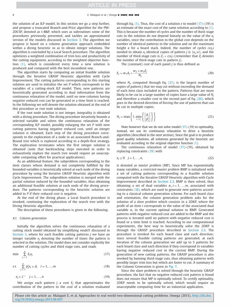
is denoted as master problem (MP). Since MP has exponentiallymany variables, a restricted master problem RMP is initialized witha set of cutting patterns corresponding to a feasible solutioncomputed with the Iterative GRASP Heuristic algorithm with CycleImprovement described in Section 2.3. RMP is then solved, thusobtaining a set of dual variables πi; i¼ 1;…;m, associated withconstraints (18), which are used to generate new patterns accord-ing to a classical column generation scheme. For each board classand orientation, the column generation problem asks for thesolution of a slave problem which consists in a 2DKP, where theprofit of an item i corresponds to the value of the associated dualvariable πi in the current optimal solution to RMP. Generatedpatterns with negative reduced cost are added to the RMP and theprocess is iterated until no pattern with negative reduced cost isfound or a time limit is reached. According to our computationalexperiments, the best way to heuristically solve the 2DKP isthrough the GRASP procedure described in Section 2.3. Theprocedure is invoked for each board class and each direction;since several feasible cutting patterns are generated, at eachiteration of the column generation we add up to 5 patterns foreach board class and each direction if they correspond to variableshaving negative reduced cost in the current RMP. During thegeneration of new cutting patterns, the GRASP procedure is alsoinvoked by banning third-stage cuts, thus obtaining patterns withpossibly larger trim loss but which are faster to cut. A summary ofthe Column Generation is given in Fig. 7.

Since the slave problem is solved through the heuristic GRASPprocedure, the fact that no negative reduced cost pattern is founddoes not ensure that MP is optimally solved. To certify optimality,2DKP needs to be optimally solved, which would require anunacceptable computing time for an industrial application.







4.2. Diving Heuristic algorithm

In order to obtain integer solutions to PM-2DCSP from thefractional solutions of RMP, we propose a Diving Heuristic algorithm.

The algorithm starts with the fractional solution obtained atthe end of the column generation phase. At each iteration, thelower bound LBðxjÞ associated with some variable(s) xj; jAP is fixedto an integer value, which determines a new RMP, ideally associatedwith a node in a Branch-and-Bound search tree (that we exploreonly partially, as previously discussed). Associated with each nodewe can define a residual demand ~di ¼maxfdi�∑jAP pijLBðxjÞ;0g,i¼1,…,m, corresponding to the items not yet included intofixed patterns. At each node, RMP is solved by column generation,unless a time limit is reached, in which case no new columns areadded to RMP. The procedure stops when the solution to RMP isinteger.

Since RMP only approximates the contribution to the objectivefunction (1) of the number of cutting cycles and third-stage cuts,the diving heuristic, through variable selection and fixing, has afundamental role in producing solutions which not only reducethe trim loss but also consider the productivity of the cuttingequipment. This is obtained by enforcing solutions where identicalcutting patterns are selected in several copies, whose number ispossibly a multiple of the maximum height κ of a board stack.

More in detail, the exploration of a generic node during theDiving Heuristic consists of three main steps

1. Solve the RMP associated with the node: RMP is solved bycolumn generation, where new columns are obtained by theGRASP procedure (see Section 2.3), which consider a residualinstance with demands ~d. If a time limit for the generation ofnew columns is reached, the algorithm just solves thecurrent RMP;

2. Heuristically solve the residual problem with demands ~d byusing the GRASP algorithm for PM-2DCSP (see Section 2.3). Let~P be the set of patterns corresponding to the residual problemsolution. These patterns are added to the set of patterns P ofRMP and, by specifying the number of times that they appear inthe solution, they define a partial solution to RMP, denoted as ~x.Hashing techniques are used to avoid the insertion of variablescorresponding to identical patterns in RMP. The partial solution~x, combined with the partial solution determined by the lowerbounds of the variables, provides an integer solution x to theRMP, namely, xj ¼ ~xj þLBðxjÞ, jAP. This solution is compared,through Eq. (1), with the best incumbent solution, which isupdated when needed.

3. One or more fractional variables are selected and their lowerbounds (LB), or lower and upper bounds (UB), are fixed to aninteger value, as discussed in the following, thus defining thenew node to be explored. Whenever the LB associated with avariable is fixed, the availability of the items is updated and theheuristics used to solve the corresponding slave problemconsiders only the residual demands ~d.

Various strategies were considered concerning the selection ofa fractional variable and the fixing of its value or of the corre-sponding lower bound LB. In our computational experiments weinvestigated the following alternatives:

1. Variable selection: (i) select the largest fractional variable, (ii)select the variable with the largest fractional part, (iii) selectthe variable with the smallest fractional part.

2. Fixing: (i) fix the variable to an integer value; (ii) set thevariable lower bound LB to an integer value.

3. Fix/bound value: (i) fix the variable (resp., set the variablelower bound LB) to its value rounded-up, (ii) fix the variable(resp., set the variable lower bound LB) to its value rounded-down (note that RMP can become infeasible when a variable isfixed to its value rounded-down and the column generation isstopped), (iii) fix the selected variable (resp., set the variablelower bound LB) to the largest integer such that the demand ofthe items in the pattern associated with the variable is notexceeded.

4. Additional variable fixing: (i) for each variable with value largerthan or equal to κ, set the lower bound of the variable to thelargest multiple of κ that does not exceed the variable value; (ii)fix the value of all the variables having integer value.

According to our computational experiments, the strategywhich gives the best results is the following: when new columnsare not generated because of a time limit in the column generationphase, we select the variable with the largest fractional part andfix it to its rounded-up value. Otherwise, we fix the variable to thelargest value that does not exceed the demand of each item classincluded in the pattern. We improve the results in terms ofnumber of cutting cycles and third stage cuts by additionallyfixing the lower bound of all the variables with value larger thanor equal to κ to the largest multiple of κ that does not exceed thevariable value.

Notice that, when the upper bound of a variable xj with currentvalue xj in RMP is set to UBðxjÞoxj , the variable may have negativereduced cost at the next iteration of the column generation phase(this surely happens if we do not change the bound of any othervariable), and thus the corresponding pattern may be generatedagain. Hashing techniques are used to check whether a variable xj,whose upper bound was set to UBðxjÞoxj has been re-generated.When this happens, the variable value is fixed at ⌈xj⌉.

Furthermore, when the time limit for the column generationphase is reached, setting the upper bound of variable xj toUBðxjÞoxj could generate unfeasibility, i.e., some items may notbe covered by any other column. To avoid this situation, we allowthe rounding down of the variables only when the time limit forthe column generation phase has not been reached.

As explained in Section 4.1, we do not solve to optimalitymodel (17)–(19), instead, we use the value of its continuousrelaxation to drive the Diving Heuristic algorithm. We could have

Fig. 7. Summary of the Column Generation procedure.







solved directly model1 or model2, however, as explained in thefollowing, the corresponding continuous relaxations would havenot been as effective in driving the algorithm.

The continuous relaxation of model1 would satisfy constraints(5) by imposing yj ¼ xj=κ for each pattern j, and thus in the objectivefunction (3) the cost vj associated with the number of cutting cycleswould be added to the objective function proportionally to thevalue of xj, without providing any useful information for guidingthe Diving Heuristic algorithm. Concerning model2, its continuousrelaxation would always select, for a specific pattern j, the variablexκjj , since this is the one having the minimum relative costsassociated with cycles and third stage cuts (these cost componentsare divided by the largest possible number of copies κj in Eq. (14)).Thus we would obtain highly fractional solutions of the continuousrelaxation, providing again little guidance to the Diving Heuristicalgorithm.

By considering model (17)–(19), we can explicitly force theRMP to privilege patterns which are likely to appear in severalcopies. This is particularly effective when matched with theselected fixing strategy, which privileges patterns appearing inmultiple copies in the RMP solution.

4.3. Post-optimization: local search procedure

Given the best incumbent solution at the end of the DivingHeuristic algorithm, the Local Search procedure (LS) partiallydestroys the solution and re-applies the Diving Heuristic algo-rithm, so as to explore a different portion of the search tree.

At each iteration of LS, a subset of the non-zero variables of thebest incumbent solution is fixed at the corresponding current(integer) value, defining a residual problem and an associatedresidual demand ~d. The Diving Heuristic algorithm is then appliedstarting from the residual problem, thus exploring a (hopefully)different region of the search tree. When calling the DivingHeuristic algorithm within the Local Search Phase, we do notgenerate new columns by explicitly solving the slave problems, butwe still heuristically solve the residual problem associated withthe nodes (and add the corresponding columns as explained inSection 4.2). LS is iteratively called, starting from the best incum-bent solution, until a time limit is reached.

The main design choice for LS concerns the decision about thevariables (i.e., the patterns) to be maintained in the incumbentsolution. The first idea we tested was to consider some optimiza-tion criterion, that is, to delete from the solution the “bad”patterns and keep the “good” part of the solution. However, ourcomputational experience showed that this choice is not effectivein diversifying the tree exploration. An explanation of this beha-vior is the following: the Diving Heuristic algorithm fixes “good”patterns at the initial nodes of the search tree, while “bad”patterns are normally fixed at the last levels; thus, deleting fromthe solution patterns of lower quality (according to some optimi-zation criterion) does not give the Diving Heuristic algorithm theopportunity to diversify the search, because the algorithm isbrought back to some node close to the bottom part of the searchtree. On the other hand, randomly choosing the variables (pat-terns) to be fixed gives the Diving Heuristic algorithm theopportunity to really diversify the search, and possibly to exploreimproving solutions.

In detail, we keep the first D percent of the non-zero variablesand set to 0 the remaining ones, according to a given ordering. Thefollowing criteria in choosing the variables (patterns) to be keptwere considered

� random ordering;� order the variables according to increasing values of the waste

in the patterns corresponding to the variables;

� order the variables according to decreasing value of a dualscore computed as the sum of the dual variables associatedwith the items included in the corresponding patterns. Thedual variables correspond to the optimal dual solution found atthe end of the root node.

As anticipated, the best strategy consists of keeping a percentage Dof the variables, which are randomly chosen.

5. Computational experiments

The above described heuristic algorithms were coded in Cþþand run on one core of an Intel Core 2 Quad at 2.50 GHz, with7.6 GB shared memory, under Linux Ubuntu 9.04 operating sys-tem. As ILP solver for the models presented in Section 3 we usedCPLEX12.1 [27]; while for the t-B&P algorithm of Section 4 we donot make use of any commercial software or component, and weuse the freeware solver GLPK 4.32 (GNU Linear Programming Kit)[26] as LP solver.

According to the opinion of the experts working in the woodcutting industry, a computing time of approximately 10 min isacceptable when looking for good quality solutions. Since the finalobjective of this research is to propose an algorithm of practicalinterest, we set the time limits of our algorithm so as to obtainglobal computing times not exceeding 10 min.

The computational experiments are designed as follows: firstwe wish to investigate which is the best among the fast heuristicalgorithms to be embedded in the t-B&B algorithm, and show theresults which can be obtained by using a straightforward integra-tion through the solution of the optimization models; second wewant to show that all the components of the proposed t-B&Balgorithm are useful in producing good quality solutions, describ-ing how the best incumbent solution is improved during thealgorithm phases; finally, the experiments will assess the perfor-mance of the proposed algorithms when compared with foureffective commercial tools available for the solution of the PM-2DCSP.

5.1. Instances generator

The algorithms were computationally tested on a set of 30realistic instances obtained by combining the dimensions andcharacteristics of a set of real world cutting problems from thewood cutting industry. The instances consider 974 item classeswith length and width in the range [108, 3512] and [65, 1606],respectively, and 24 board classes with length and width in therange [1844, 5300] and [1020, 2200], respectively. All the itemscan be rotated and the maximum number κ of boards which canbe stacked in a pile and cut with a single cycle is set to 6.

Every instance is defined by the total number of items t, withtAf25; 50; 75; 100; 150; 200; 300; 400; 600; 800g, the numberof item classes m, with mAf10; 40; 80g and the number of boardclasses b, with bAf2;3g. The number of board classes is set to twofor all the combinations; for the larger combinations we createdadditional instances with three board classes. The name of eachinstance defines its features in terms of board class number, itemclass number and item number: b-mxt.

Starting from a set of real world instances, we obtain a list ofitems which is used to generate our instances. A main feature ofthe real world problems from the wood cutting industry is that theitems have correlated dimensions: for example, a rectangular itemused as back of a closet has one dimension in common with thetwo rectangular items used as doors. In order to obtain instanceswith this feature by considering the real world instances, wedefine an adjacency graph G¼ ðV ; EÞ where there is one vertex for







every item class and the edges connect item classes having onedimension in common.

When generating an instance, the first item class (vertex) israndomly selected and the corresponding vertex is marked asunavailable. Then, with a probability equal to 0.7, the next itemclass is randomly selected among the available adjacent classes(vertices). With a probability equal to 0.3 the next item class(vertex) is randomly selected among all the available classes. Thesame random selection is performed when the last selected itemclass has no available adjacent vertex in the graph. The selectionstep is iterated until m item classes have been created.

In order to define the demand di associated with the m selecteditem classes, we first set di¼1, i¼1,…,m. Then, iteratively, werandomly select an item class and increase its demand of one unit.We stop when t items are globally obtained. The dimensions of theboard classes are randomly selected among the real world boarddimensions and we check that all the item classes fit into at leastone board class (otherwise the last selected board class isdiscarded and a new random choice is performed).

5.2. Setting of the algorithms

The weights w1, w2 and w3 used in the objective function (1)(where A is expressed in square meters) are given in Table 1. Theseweights are set according to the expert opinion of people workingin the wood cutting industry, and tend to give a large importanceto the trim loss minimization, but at the same time recognize thatproductivity cannot be ignored. Clearly a different objective func-tion would produce different results, in particular for what con-cerns the optimization models and the Diving Heuristic algorithm.

Table 1 also reports the other parameters mentioned in thepaper: the coefficients β and γ used in the Strip Heuristic algo-rithm, for which we tested βA ½0; 5; 10; 15; 20; 25� andγA ½0; 5; 10; 15; 20; 25�; the percentage of variables to be keptin LS, for which we considered DA ½20; 30; 40; 50; 60; 70�; andthe time limits for the column generation phase and the LocalSearch procedure (LS). Each parameter value was chosen byselecting the one giving the best average results according to ourcomputational experiments; for the time limits, as we said, we hadthe limitation of not exceeding 10 min of global computing time:we stop the generation of new columns after 500 s and, after theDiving Heuristic algorithm, we run the Local Search procedure LSfor at most 100 s.

5.3. Heuristic algorithms and hybrid method

This section reports the results obtained with the 3 heuristicalgorithms (described in Sections 2.1, 2.2 and 2.3), which are runwith and without the cycle improvement procedure (described inSection 2.4), thus obtaining 6 possible configurations. In addition,we solved the models proposed in Section 3 by defining onecutting pattern for each pattern generated by the 4 best perform-ing algorithms among the 6 configurations (corresponding to

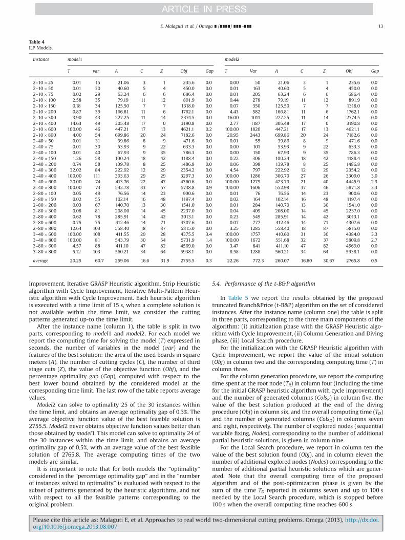
1 variable for model1 and, at most, κ variables for model2). InTables 2, 3 and 4, for each computed solution we report the totalarea of the used boards, the number of cutting cycles and thenumber of third stage cuts.

In Table 2 we report the results obtained by the heuristicalgorithms in the iterative configuration (without the cycleimprovement procedure). After the instance name (column 1),the table is split in three parts, corresponding to the Strip Heuristicalgorithm, the Iterative Multi-Pattern Heuristic algorithm and theIterative GRASP Heuristic algorithm, respectively. For each algo-rithm we give the computing time (T) expressed in seconds, thearea of the used boards in square meters (A), the number of cuttingcycles (C), the number of third stage cuts (Z) and the value of theobjective function (Obj). The same information is reported inTable 3 for the configuration which tries to reduce the numberof cycles. The last rows of the tables report average values.

Comparing the average results obtained by the heuristic algo-rithms in the iterative configuration (we refer to the averagevalues from Table 2), the best performing one is the IterativeGRASP Heuristic algorithm, which needs 261.49 m2 of raw mate-rial, 29.8 cutting cycles and 43.8 third stage cuts, with an objectivefunction value of 2897.3. This algorithm is the most expensive onefrom the computational viewpoint, requiring 29.15 s. With respectto the Iterative GRASP Heuristic algorithm, the Iterative Multi-Pattern Heuristic algorithm obtains an objective function value of3013.7, mainly due to an increase of approximately 13 m2 of rawmaterial, while the number of cutting cycles is almost the sameand the number of third stage cuts is reduced to 23.6; thecomputing time is approximately the fourth (7.13 s). The StripHeuristic algorithm obtains an objective function value of 3063.8;it needs almost the same raw material used by the Iterative Multi-Pattern Heuristic algorithm, but approximately 5 more cuttingcycles and 3 more third stage cuts, with a computing time of18.55 s.

When the cycle improvement configuration is used (we refer tothe average values from Table 3), the main effect that we canobserve is a reduction in the number of cutting cycles, whichconfirms the efficacy of the procedure. As a side effect, we alsoobserve a reduction in the number of third stage cuts, which iscorrelated to the number of cutting cycles because the third stagecuts are counted per cycle (and not per board). Another importantside effect is a notable reduction of the computing times of thealgorithms, due to the fact that smaller problems are solved ateach iteration. Concerning the single algorithms, the best perform-ing one is still the GRASP Heuristic algorithm, with a smallincrease in the need of raw material (265.21 m2), while thenumber of cutting cycles is halved (14.5) and the third stage cutsare reduced to 30.1, with an objective function value of 2798.2. Inthis version the algorithm is very fast, requiring only 2.35 s ofaverage computing time. The Strip Heuristic algorithm is thesecond best algorithm, obtaining an objective function value of2973.5. In this configuration, the algorithm obtains an approxi-mate reduction of 3 m2 of raw material, while the number ofcutting cycles is reduced of 7 units and the number of third stagecuts is reduced of 4 units. The computing time is approximatelyhalved to 8.25 s. The Iterative Multi-Pattern Heuristic algorithmobtains a slightly improved performance in this version, with anobjective function value of 3010.3; it needs approximately 10additional m2 of raw material but the number of cutting cycles ishalved (16.4) with approximately the same number of 3 thirdstage cuts. The computing time reduces to 0.36 s.

Table 4 reports the results obtained by solving model1 andmodel2 with a time limit of 100 s each. The models are initializedby defining a variable (or up to κ variables for model2) for eachcutting pattern generated by the 4 best performing heuristicalgorithms, namely Iterative GRASP Heuristic algorithm with Cycle

Table 1Parameters of the algorithms.

Parameter Value

w1 10w2 8w3 1β 15γ 5Column generation time limit 500 sLS time limit 100 sLS variables to be kept (D) 30







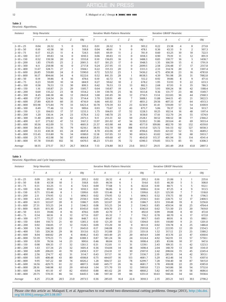
Table 2Heuristic Algorithms.

Instance Strip Heuristic Iterative Multi-Pattern Heuristic Iterative GRASP Heuristic

T A C Z Obj T A C Z Obj T A C Z Obj

2–10�25 0.04 26.32 5 0 303.2 0.01 26.32 5 0 303.2 0.22 23.38 4 8 273.82–10�50 0.10 43.58 10 3 518.8 0.04 40.61 9 0 478.1 0.36 43.33 9 2 507.32–10�75 0.17 63.25 11 4 724.5 0.05 69.19 11 2 781.9 0.60 63.25 10 10 722.52–10�100 0.17 89.83 14 0 1010.3 0.06 89.83 15 0 1018.3 0.90 79.19 11 12 891.92–10�150 0.52 139.58 20 0 1555.8 0.10 136.03 16 0 1488.3 0.85 130.77 16 3 1438.72–10�200 1.85 179.95 25 2 2001.5 0.17 181.25 17 0 1948.5 1.35 166.59 15 6 1791.92–10�300 4.11 258.98 16 0 2717.8 0.24 257.95 15 0 2699.5 2.58 236.48 17 17 2517.82–10�400 11.67 328.71 27 1 3504.1 0.22 315.33 20 0 3313.3 2.33 314.74 20 0 3307.42–10�600 26.85 519.80 24 0 5390.0 0.72 523.52 25 1 5436.2 4.75 458.38 23 16 4783.82–10�800 16.17 894.66 34 4 9222.6 0.52 841.35 28 1 8638.5 4.39 761.98 29 31 7882.82–40�50 0.19 39.86 8 16 478.6 0.10 42.72 9 13 512.2 0.92 39.86 8 9 471.62–40�75 0.23 59.09 10 14 684.9 0.27 59.62 10 2 678.2 1.95 53.93 9 22 633.32–40�100 0.58 76.53 13 30 899.3 0.42 76.53 13 13 882.3 2.68 67.93 9 35 786.32–40�150 1.16 110.87 21 29 1305.7 0.64 110.87 19 4 1264.7 5.93 100.24 18 42 1188.42–40�200 0.69 135.22 23 18 1554.2 1.59 139.78 25 16 1613.8 9.36 131.77 23 48 1549.72–40�300 8.45 246.38 46 12 2843.8 3.68 241.65 36 12 2716.5 13.14 222.83 36 44 2560.32–40�400 17.87 324.54 56 21 3714.4 3.70 320.91 49 7 3608.1 11.88 344.15 45 21 3822.52–40�600 27.89 420.19 60 35 4716.9 6.66 441.02 53 17 4851.2 29.56 407.33 47 64 4513.32–40�800 103.98 575.84 79 33 6423.4 10.78 570.39 63 23 6230.9 41.41 559.09 57 54 6100.92–80�100 0.49 77.46 13 31 909.6 0.93 73.67 12 43 875.7 5.06 78.37 12 34 913.72–80�150 1.21 104.03 17 57 1233.3 1.75 104.03 17 52 1228.3 10.25 102.14 16 48 1197.42–80�200 1.20 136.14 24 23 1576.4 3.12 140.70 25 31 1638.0 17.10 132.79 24 55 1574.92–80�300 11.40 208.55 41 62 2475.5 9.11 213.31 42 59 2528.1 30.52 198.52 38 77 2366.22–80�400 6.17 273.82 47 53 3167.2 13.97 281.02 47 34 3220.2 51.86 263.64 41 69 3033.42–80�600 10.56 412.09 51 73 4601.9 21.57 413.90 44 86 4577.0 109.86 402.70 50 132 4559.02–80�800 36.43 552.91 76 79 6216.1 38.55 552.70 60 108 6115.0 125.72 541.53 62 127 6038.33–40�600 33.33 430.38 65 24 4847.8 8.70 432.06 47 10 4706.6 39.03 421.82 52 55 4689.23–40�800 113.45 553.80 76 34 6180.0 12.18 557.05 53 30 6024.5 63.82 542.17 58 68 5953.73–80�600 21.75 412.98 56 87 4664.8 25.81 419.60 47 71 4643.0 115.37 401.94 51 114 4541.43–80�800 97.78 559.85 102 56 6470.5 48.23 571.03 76 72 6390.3 170.85 553.73 85 91 6308.3

Average 18.55 275.17 35.7 26.7 3063.8 7.13 274.80 30.3 23.6 3013.7 29.15 261.49 29.8 43.8 2897.3

Table 3Heuristic Algorithms and Cycle Improvement.

Instance Strip Heuristic Iterative Multi-Pattern Heuristic Iterative GRASP Heuristic

T A C Z Obj T A C Z Obj T A C Z Obj

2–10�25 0.09 26.32 4 0 295.2 0.02 26.32 4 0 295.2 0.16 21.06 3 1 235.62–10�50 0.18 43.58 10 3 518.8 0.01 46.56 6 1 514.6 0.15 46.30 5 5 508.02–10�75 0.31 63.25 11 4 724.5 0.00 77.68 5 6 822.8 0.10 88.71 5 5 932.12–10�100 0.26 89.83 14 0 1010.3 0.01 96.06 6 0 1008.6 0.14 87.25 4 9 913.52–10�150 0.71 133.46 8 1 1399.6 0.01 133.46 8 1 1399.6 0.21 125.50 7 7 1318.02–10�200 2.11 179.95 12 1 1896.5 0.02 179.95 12 1 1896.5 0.32 170.75 10 9 1796.52–10�300 4.33 245.25 12 10 2558.5 0.04 245.25 12 10 2558.5 0.61 228.75 12 17 2400.52–10�400 14.13 322.67 20 0 3386.7 0.05 322.67 20 0 3386.7 0.53 310.48 19 0 3256.82–10�600 27.31 515.25 24 2 5346.5 0.08 515.25 24 2 5346.5 0.85 459.54 18 25 4764.42–10�800 16.01 815.30 24 0 8345.0 0.05 819.70 23 1 8382.0 0.62 721.50 23 20 7419.02–40�50 0.33 39.86 8 16 478.6 0.09 42.70 7 9 492.0 0.99 39.88 8 10 472.82–40�75 0.54 60.16 8 12 677.6 0.07 65.32 7 7 716.2 0.78 60.70 6 17 672.02–40�100 0.77 72.27 12 30 848.7 0.11 89.47 11 11 993.7 0.65 80.91 8 15 888.12–40�150 0.84 110.73 21 10 1285.3 0.10 121.20 10 12 1304.0 0.91 110.80 9 21 1201.02–40�200 0.92 138.05 17 12 1528.5 0.09 172.29 10 9 1811.9 0.92 139.78 8 25 1486.82–40�300 3.36 246.20 22 7 2645.0 0.17 246.08 15 13 2593.8 1.27 222.95 12 29 2354.52–40�400 7.65 326.36 29 18 3513.6 0.23 312.88 25 23 3351.8 1.52 317.12 23 25 3380.22–40�600 8.04 440.82 29 6 4646.2 0.43 443.49 25 20 4654.9 3.00 413.76 22 47 4360.62–40�800 53.39 579.23 71 28 6388.3 0.87 581.24 36 24 6124.4 4.92 542.91 33 57 5750.12–80�100 0.59 76.56 14 23 900.6 0.46 88.84 13 16 1008.4 2.85 83.06 10 37 947.62–80�150 0.98 109.35 17 32 1261.5 0.31 112.01 11 31 1239.1 2.43 109.35 11 42 1223.52–80�200 1.63 137.34 25 32 1605.4 0.36 154.84 14 38 1698.4 2.04 140.70 13 30 1541.02–80�300 6.09 206.03 41 70 2458.3 0.37 234.10 17 30 2507.0 2.42 208.04 15 45 2245.42–80�400 2.56 274.77 42 31 3114.7 0.43 317.17 16 37 3336.7 2.19 285.91 14 42 3013.12–80�600 5.05 408.48 43 80 4508.8 0.75 444.07 16 113 4681.7 5.29 412.46 14 71 4307.62–80�800 9.95 547.22 60 74 6026.2 1.28 604.57 22 78 6299.7 7.28 558.40 18 87 5815.03–40�600 14.56 429.75 61 22 4807.5 0.60 445.77 26 16 4681.7 3.78 418.08 22 29 4385.83–40�800 28.16 548.98 62 29 6014.8 1.04 571.70 33 12 5993.0 7.23 543.86 30 54 5732.63–80�600 6.94 411.10 47 82 4569.0 0.88 461.62 20 84 4860.2 5.82 447.66 19 58 4686.63–80�800 29.75 570.35 86 54 6445.5 1.88 597.30 39 66 6351.0 10.63 560.26 34 64 5938.6

Average 8.25 272.28 28.5 23.0 2973.5 0.36 285.65 16.4 22.4 3010.3 2.35 265.21 14.5 30.1 2798.2







Improvement, Iterative GRASP Heuristic algorithm, Strip Heuristicalgorithm with Cycle Improvement, Iterative Multi-Pattern Heur-istic algorithm with Cycle Improvement. Each heuristic algorithmis executed with a time limit of 15 s, when a complete solution isnot available within the time limit, we consider the cuttingpatterns generated up-to the time limit.

After the instance name (column 1), the table is split in twoparts, corresponding to model1 and model2. For each model wereport the computing time for solving the model (T) expressed inseconds, the number of variables in the model (var) and thefeatures of the best solution: the area of the used boards in squaremeters (A), the number of cutting cycles (C), the number of thirdstage cuts (Z), the value of the objective function (Obj), and thepercentage optimality gap (Gap), computed with respect to thebest lower bound obtained by the considered model at thecorresponding time limit. The last row of the table reports averagevalues.

Model2 can solve to optimality 25 of the 30 instances withinthe time limit, and obtains an average optimality gap of 0.3%. Theaverage objective function value of the best feasible solution is2755.5. Model2 never obtains objective function values better thanthose obtained by model1. This model can solve to optimality 24 ofthe 30 instances within the time limit, and obtains an averageoptimality gap of 0.5%, with an average value of the best feasiblesolution of 2765.8. The average computing times of the twomodels are similar.

It is important to note that for both models the “optimality”considered in the “percentage optimality gap” and in the “numberof instances solved to optimality” is evaluated with respect to thesubset of patterns generated by the heuristic algorithms, and notwith respect to all the feasible patterns corresponding to theoriginal problem.

5.4. Performance of the t-B&P algorithm

In Table 5 we report the results obtained by the proposedtruncated Branch&Price (t-B&P) algorithm on the set of consideredinstances. After the instance name (column one) the table is splitin three parts, corresponding to the three main components of thealgorithm: (i) initialization phase with the GRASP Heuristic algo-rithm with Cycle Improvement, (ii) Column Generation and Divingphase, (iii) Local Search procedure.

For the initialization with the GRASP Heuristic algorithm withCycle Improvement, we report the value of the initial solution(Obj) in column two and the corresponding computing time (T) incolumn three.

For the column generation procedure, we report the computingtime spent at the root node (TR) in column four (including the timefor the initial GRASP heuristic algorithm with cycle improvement)and the number of generated columns (ColsR) in column five, thevalue of the best solution produced at the end of the divingprocedure (Obj) in column six, and the overall computing time (TD)and the number of generated columns (ColsD) in columns sevenand eight, respectively. The number of explored nodes (sequentialvariable fixing, Nodes), corresponding to the number of additionalpartial heuristic solutions, is given in column nine.

For the Local Search procedure, we report in column ten thevalue of the best solution found (Obj), and in column eleven thenumber of additional explored nodes (Nodes) corresponding to thenumber of additional partial heuristic solutions which are gener-ated. Note that the overall computing time of the proposedalgorithm and of the post-optimization phase is given by thesum of the time TD reported in columns seven and up to 100 sneeded by the Local Search procedure, which is stopped before100 s when the overall computing time reaches 600 s.

Table 4ILP Models.

instance model1 model2

T var A C Z Obj Gap T Var A C Z Obj Gap

2–10�25 0.01 15 21.06 3 1 235.6 0.0 0.00 50 21.06 3 1 235.6 0.02–10�50 0.01 30 40.60 5 4 450.0 0.0 0.01 163 40.60 5 4 450.0 0.02–10�75 0.02 29 63.24 6 6 686.4 0.0 0.01 205 63.24 6 6 686.4 0.02–10�100 2.58 35 79.19 11 12 891.9 0.0 0.44 278 79.19 11 12 891.9 0.02–10�150 0.18 34 125.50 7 7 1318.0 0.0 0.07 350 125.50 7 7 1318.0 0.02–10�200 0.87 39 166.81 11 6 1762.1 0.0 4.43 582 166.81 11 6 1762.1 0.02–10�300 3.90 43 227.25 11 14 2374.5 0.0 16.00 1011 227.25 11 14 2374.5 0.02–10�400 14.63 49 305.48 17 0 3190.8 0.0 2.77 1187 305.48 17 0 3190.8 0.02–10�600 100.00 46 447.21 17 13 4621.1 0.2 100.00 1820 447.21 17 13 4621.1 0.62–10�800 4.00 54 699.86 20 24 7182.6 0.0 20.95 2443 699.86 20 24 7182.6 0.02–40�50 0.01 31 39.86 8 9 471.6 0.0 0.01 55 39.86 8 9 471.6 0.02–40�75 0.01 30 53.93 9 22 633.3 0.0 0.00 101 53.93 9 22 633.3 0.02–40�100 0.01 40 67.93 9 35 786.3 0.0 0.00 150 67.93 9 35 786.3 0.02–40�150 1.26 58 100.24 18 42 1188.4 0.0 0.22 306 100.24 18 42 1188.4 0.02–40�200 0.74 58 139.78 8 25 1486.8 0.0 0.06 398 139.78 8 25 1486.8 0.02–40�300 32.02 84 222.92 12 29 2354.2 0.0 4.54 797 222.92 12 29 2354.2 0.02–40�400 100.00 111 303.63 29 29 3297.3 3.0 100.00 1286 306.70 27 26 3309.0 3.02–40�600 20.00 74 413.76 22 47 4360.6 0.0 100.00 1279 423.79 21 40 4445.9 2.32–40�800 100.00 74 542.78 33 57 5748.8 0.9 100.00 1606 552.98 37 46 5871.8 3.32–80�100 0.05 49 76.56 14 23 900.6 0.0 0.01 76 76.56 14 23 900.6 0.02–80�150 0.02 55 102.14 16 48 1197.4 0.0 0.02 164 102.14 16 48 1197.4 0.02–80�200 0.03 67 140.70 13 30 1541.0 0.0 0.01 284 140.70 13 30 1541.0 0.02–80�300 0.08 81 208.00 14 45 2237.0 0.0 0.04 409 208.00 14 45 2237.0 0.02–80�400 0.62 78 285.91 14 42 3013.1 0.0 0.23 549 285.91 14 42 3013.1 0.02–80�600 0.75 75 412.46 14 71 4307.6 0.0 0.07 777 412.46 14 71 4307.6 0.02–80�800 12.64 103 558.40 18 87 5815.0 0.0 3.25 1285 558.40 18 87 5815.0 0.03–40�600 100.00 108 411.55 29 28 4375.5 3.4 100.00 1757 410.60 31 30 4384.0 3.33–40�800 100.00 81 543.79 30 54 5731.9 1.4 100.00 1672 551.68 32 37 5809.8 2.73–80�600 4.57 88 411.10 47 82 4569.0 0.0 3.47 841 411.10 47 82 4569.0 0.03–80�800 5.12 103 560.21 34 64 5938.1 0.0 8.58 1288 560.21 34 64 5938.1 0.0

average 20.25 60.7 259.06 16.6 31.9 2755.5 0.3 22.26 772.3 260.07 16.80 30.67 2765.8 0.5







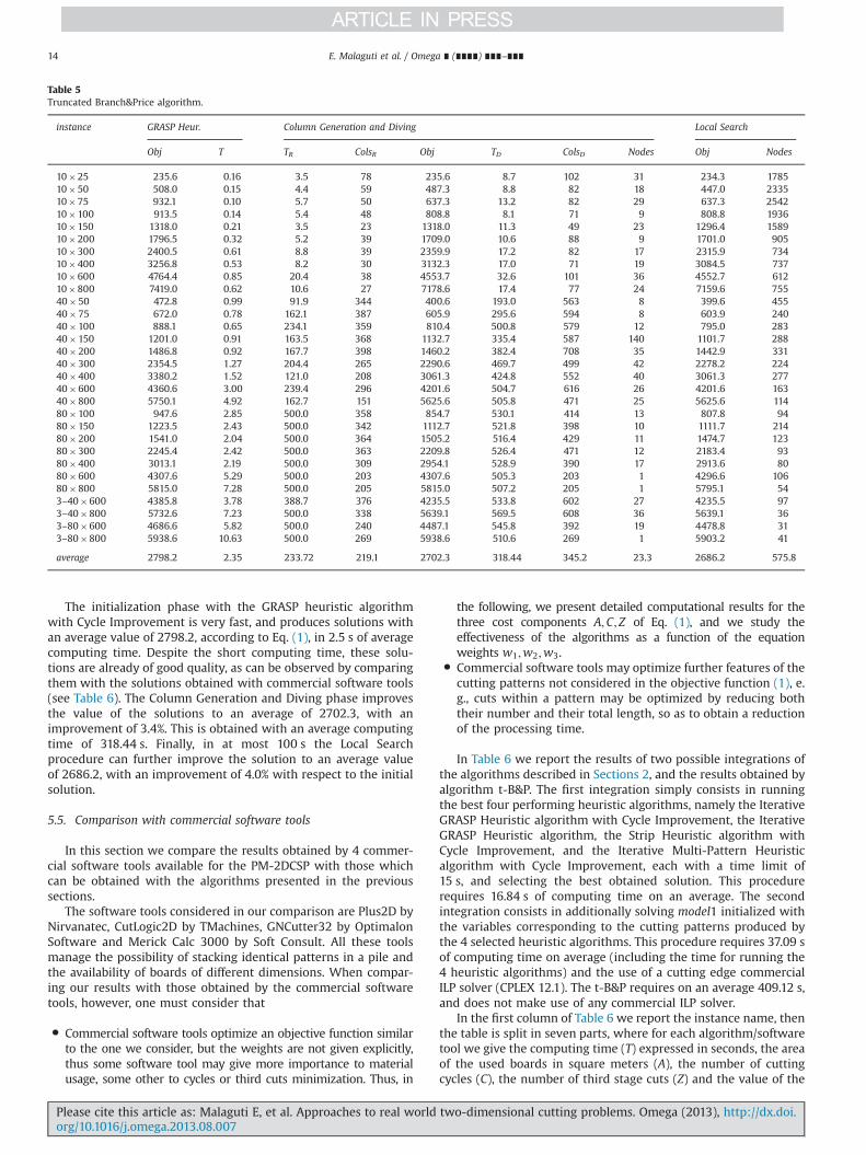
The initialization phase with the GRASP heuristic algorithmwith Cycle Improvement is very fast, and produces solutions withan average value of 2798.2, according to Eq. (1), in 2.5 s of averagecomputing time. Despite the short computing time, these solu-tions are already of good quality, as can be observed by comparingthem with the solutions obtained with commercial software tools(see Table 6). The Column Generation and Diving phase improvesthe value of the solutions to an average of 2702.3, with animprovement of 3.4%. This is obtained with an average computingtime of 318.44 s. Finally, in at most 100 s the Local Searchprocedure can further improve the solution to an average valueof 2686.2, with an improvement of 4.0% with respect to the initialsolution.

5.5. Comparison with commercial software tools

In this section we compare the results obtained by 4 commer-cial software tools available for the PM-2DCSP with those whichcan be obtained with the algorithms presented in the previoussections.

The software tools considered in our comparison are Plus2D byNirvanatec, CutLogic2D by TMachines, GNCutter32 by OptimalonSoftware and Merick Calc 3000 by Soft Consult. All these toolsmanage the possibility of stacking identical patterns in a pile andthe availability of boards of different dimensions. When compar-ing our results with those obtained by the commercial softwaretools, however, one must consider that

� Commercial software tools optimize an objective function similarto the one we consider, but the weights are not given explicitly,thus some software tool may give more importance to materialusage, some other to cycles or third cuts minimization. Thus, in

the following, we present detailed computational results for thethree cost components A;C; Z of Eq. (1), and we study theeffectiveness of the algorithms as a function of the equationweights w1;w2;w3.� Commercial software tools may optimize further features of thecutting patterns not considered in the objective function (1), e.g., cuts within a pattern may be optimized by reducing boththeir number and their total length, so as to obtain a reductionof the processing time.

In Table 6 we report the results of two possible integrations ofthe algorithms described in Sections 2, and the results obtained byalgorithm t-B&P. The first integration simply consists in runningthe best four performing heuristic algorithms, namely the IterativeGRASP Heuristic algorithm with Cycle Improvement, the IterativeGRASP Heuristic algorithm, the Strip Heuristic algorithm withCycle Improvement, and the Iterative Multi-Pattern Heuristicalgorithm with Cycle Improvement, each with a time limit of15 s, and selecting the best obtained solution. This procedurerequires 16.84 s of computing time on an average. The secondintegration consists in additionally solving model1 initialized withthe variables corresponding to the cutting patterns produced bythe 4 selected heuristic algorithms. This procedure requires 37.09 sof computing time on average (including the time for running the4 heuristic algorithms) and the use of a cutting edge commercialILP solver (CPLEX 12.1). The t-B&P requires on an average 409.12 s,and does not make use of any commercial ILP solver.

In the first column of Table 6 we report the instance name, thenthe table is split in seven parts, where for each algorithm/softwaretool we give the computing time (T) expressed in seconds, the areaof the used boards in square meters (A), the number of cuttingcycles (C), the number of third stage cuts (Z) and the value of the

Table 5Truncated Branch&Price algorithm.

instance GRASP Heur. Column Generation and Diving Local Search

Obj T TR ColsR Obj TD ColsD Nodes Obj Nodes

10�25 235.6 0.16 3.5 78 235.6 8.7 102 31 234.3 178510�50 508.0 0.15 4.4 59 487.3 8.8 82 18 447.0 233510�75 932.1 0.10 5.7 50 637.3 13.2 82 29 637.3 254210�100 913.5 0.14 5.4 48 808.8 8.1 71 9 808.8 193610�150 1318.0 0.21 3.5 23 1318.0 11.3 49 23 1296.4 158910�200 1796.5 0.32 5.2 39 1709.0 10.6 88 9 1701.0 90510�300 2400.5 0.61 8.8 39 2359.9 17.2 82 17 2315.9 73410�400 3256.8 0.53 8.2 30 3132.3 17.0 71 19 3084.5 73710�600 4764.4 0.85 20.4 38 4553.7 32.6 101 36 4552.7 61210�800 7419.0 0.62 10.6 27 7178.6 17.4 77 24 7159.6 75540�50 472.8 0.99 91.9 344 400.6 193.0 563 8 399.6 45540�75 672.0 0.78 162.1 387 605.9 295.6 594 8 603.9 24040�100 888.1 0.65 234.1 359 810.4 500.8 579 12 795.0 28340�150 1201.0 0.91 163.5 368 1132.7 335.4 587 140 1101.7 28840�200 1486.8 0.92 167.7 398 1460.2 382.4 708 35 1442.9 33140�300 2354.5 1.27 204.4 265 2290.6 469.7 499 42 2278.2 22440�400 3380.2 1.52 121.0 208 3061.3 424.8 552 40 3061.3 27740�600 4360.6 3.00 239.4 296 4201.6 504.7 616 26 4201.6 16340�800 5750.1 4.92 162.7 151 5625.6 505.8 471 25 5625.6 11480�100 947.6 2.85 500.0 358 854.7 530.1 414 13 807.8 9480�150 1223.5 2.43 500.0 342 1112.7 521.8 398 10 1111.7 21480�200 1541.0 2.04 500.0 364 1505.2 516.4 429 11 1474.7 12380�300 2245.4 2.42 500.0 363 2209.8 526.4 471 12 2183.4 9380�400 3013.1 2.19 500.0 309 2954.1 528.9 390 17 2913.6 8080�600 4307.6 5.29 500.0 203 4307.6 505.3 203 1 4296.6 10680�800 5815.0 7.28 500.0 205 5815.0 507.2 205 1 5795.1 543–40�600 4385.8 3.78 388.7 376 4235.5 533.8 602 27 4235.5 973–40�800 5732.6 7.23 500.0 338 5639.1 569.5 608 36 5639.1 363–80�600 4686.6 5.82 500.0 240 4487.1 545.8 392 19 4478.8 313–80�800 5938.6 10.63 500.0 269 5938.6 510.6 269 1 5903.2 41

average 2798.2 2.35 233.72 219.1 2702.3 318.44 345.2 23.3 2686.2 575.8







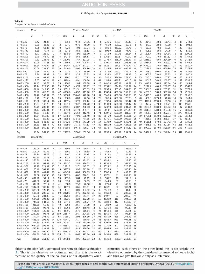
objective function (Obj), computed according to objective function(1). This is the objective we optimize, and thus it is the exactmeasure of the quality of the solutions of our algorithms when

compared each other; on the other hand, this is not strictly theobjective optimized by the considered commercial software tools,and thus we give this value only as a reference.

Table 6Comparison with commercial software.

Instance Heur. Heur. þ Model1 t�B&P Plus2D

T A C Z Obj T A C Z Obj T A C Z Obj T A C Z Obj

2–10�25 0.42 21.06 3 1 235.6 0.42 21.06 3 1 235.6 109.04 20.43 3 6 234.3 3.00 20.43 3 16 244.32–10�50 0.69 43.33 9 2 507.3 0.70 40.60 5 4 450.0 109.02 40.10 5 6 447.0 2.00 43.08 7 18 504.82–10�75 1.00 63.25 10 10 722.5 1.02 63.24 6 6 686.4 113.32 57.73 7 4 637.3 7.00 63.25 7 30 718.52–10�100 1.30 79.19 11 12 891.9 3.88 79.19 11 12 891.9 108.55 74.78 7 5 808.8 4.00 74.78 7 33 836.82–10�150 1.77 125.50 7 7 1318.0 1.95 125.50 7 7 1318.0 111.45 124.64 6 2 1296.4 3.00 124.64 14 41 1399.42–10�200 3.79 166.59 15 6 1791.9 4.66 166.81 11 6 1762.1 110.8 160.90 10 12 1701.0 3.00 161.12 15 36 1767.22–10�300 7.57 228.75 12 17 2400.5 11.47 227.25 11 14 2374.5 118.06 221.59 11 12 2315.9 4.00 224.59 16 39 2412.92–10�400 17.00 310.48 19 0 3256.8 31.63 305.48 17 0 3190.8 118.5 296.25 15 2 3084.5 1.00 299.92 19 15 3166.22–10�600 21.24 459.54 18 25 4764.4 122.39 447.21 17 13 4621.1 134.9 439.77 17 19 4552.7 3.00 439.77 21 75 4640.72–10�800 20.09 721.50 23 20 7419.0 24.09 699.86 20 24 7182.6 118.14 699.86 18 17 7159.6 5.00 699.86 25 78 7276.62–40�50 2.28 39.86 8 9 471.6 2.29 39.86 8 9 471.6 293.5 34.16 6 10 399.6 60.00 34.16 6 38 427.62–40�75 3.26 53.93 9 22 633.3 3.26 53.93 9 22 633.3 395.92 53.39 7 14 603.9 75.00 53.93 8 37 640.32–40�100 4.11 67.93 9 35 786.3 4.12 67.93 9 35 786.3 599.96 72.20 6 25 795.0 66.00 67.97 10 63 822.72–40�150 7.65 100.24 18 42 1188.4 8.91 100.24 18 42 1188.4 436.71 100.17 10 20 1101.7 54.00 100.27 18 87 1233.72–40�200 11.10 139.78 8 25 1486.8 11.84 139.78 8 25 1486.8 483.12 134.59 9 25 1442.9 50.00 127.84 20 76 1514.42–40�300 17.74 222.95 12 29 2354.5 49.76 222.92 12 29 2354.2 574.79 213.52 14 31 2278.2 40.00 200.87 28 135 2367.72–40�400 21.14 312.88 25 23 3351.8 121.51 303.63 29 29 3297.3 537.47 284.03 23 37 3061.3 46.00 287.18 51 94 3373.82–40�600 26.92 413.76 22 47 4360.6 46.92 413.76 22 47 4360.6 600.00 399.56 21 38 4201.6 56.00 387.26 36 161 4321.62–40�800 37.72 542.91 33 57 5750.1 138.40 542.78 33 57 5748.8 600.00 533.96 29 54 5625.6 44.00 525.12 51 199 5858.22–80�100 8.78 76.56 14 23 900.6 8.83 76.56 14 23 900.6 600.00 70.78 9 28 807.8 227.00 70.78 10 57 844.82–80�150 13.68 102.14 16 48 1197.4 13.70 102.14 16 48 1197.4 600.00 99.47 10 37 1111.7 259.00 97.58 15 88 1183.82–80�200 19.24 140.70 13 30 1541.0 19.27 140.70 13 30 1541.0 600.00 134.47 12 34 1474.7 247.00 128.71 21 113 1568.12–80�300 23.79 208.04 15 45 2245.4 23.87 208.00 14 45 2237.0 600.00 201.54 15 48 2183.4 238.00 193.02 33 137 2331.22–80�400 21.12 285.91 14 42 3013.1 21.74 285.91 14 42 3013.1 600.00 276.26 14 39 2913.6 278.00 257.38 36 159 3020.82–80�600 25.77 412.46 14 71 4307.6 26.52 412.46 14 71 4307.6 600.00 411.56 14 69 4296.6 225.00 392.94 41 279 4536.42–80�800 35.34 558.40 18 87 5815.0 47.98 558.40 18 87 5815.0 600.00 552.81 21 99 5795.1 253.00 526.72 48 303 5954.23–40�600 33.87 418.08 22 29 4385.8 134.48 411.55 29 28 4375.5 600.00 398.65 26 41 4235.5 64.00 356.81 37 190 4054.13–40�800 39.86 543.86 30 54 5732.6 140.52 543.79 30 54 5731.9 600.00 536.71 29 40 5639.1 57.00 521.42 48 191 5789.23–80�600 31.18 411.10 47 82 4569.0 35.75 411.10 47 82 4569.0 600.00 424.98 20 69 4478.8 171.00 391.14 44 251 4514.43–80�800 45.66 560.26 34 64 5938.6 50.78 560.21 34 64 5938.1 600.00 557.42 33 65 5903.2 207.00 529.66 66 295 6119.6

Avg. 16.84 261.03 17 32 2777.9 37.09 259.06 16 32 2755.5 409.12 254.21 14 30 2686.2 91.73 246.74 25 111 2781.5

Instance CutLogic2D GNCutter32 MerickC.3000

T A C Z Obj T A C Z Obj T A C

2–10�25 69.00 21.06 4 8 250.6 1.45 20.43 3 3 231.3 3 21.06 42–10�50 201.00 40.35 7 7 466.5 1.33 40.35 5 0 443.5 2 40.35 82–10�75 76.80 57.72 7 7 640.2 3.25 75.13 9 2 825.3 7 54.75 62–10�100 310.20 74.78 7 9 812.8 2.23 87.25 7 0 928.5 7 79.19 122–10�150 270.60 124.64 11 14 1348.4 3.38 131.62 9 0 1388.2 4 125.50 152–10�200 154.20 162.87 13 13 1745.7 2.89 176.23 12 1 1859.3 3 169.23 162–10�300 88.20 224.02 15 21 2381.2 2.17 242.62 12 2 2524.2 8 226.55 162–10�400 65.40 304.89 20 19 3227.9 3.95 313.28 21 28 3328.8 1 310.46 242–10�600 82.80 444.41 20 41 4645.1 4.03 506.89 29 6 5306.9 7 453.50 222–10�800 72.00 699.86 20 29 7187.6 6.02 776.81 26 0 7976.1 11 699.86 282–40�50 487.20 34.16 6 20 409.6 3.64 42.72 9 2 501.2 16 34.16 62–40�75 441.60 52.31 9 20 615.1 1.83 56.09 7 28 644.9 37 53.93 92–40�100 514.20 72.16 7 41 818.6 2.58 76.68 11 17 871.8 79 68.04 122–40�150 1332.60 100.07 17 51 1187.7 3.66 111.01 13 18 1232.1 67 100.21 172–40�200 679.20 127.84 22 40 1494.4 3.09 137.42 15 16 1510.2 91 131.30 202–40�300 508.80 208.53 23 59 2328.3 3.75 222.42 21 68 2460.2 93 208.50 302–40�400 453.60 291.40 27 45 3175.0 3.56 317.81 37 23 3497.1 27 292.59 412–40�600 604.20 394.83 38 70 4322.3 4.22 432.29 31 59 4629.9 116 394.66 382–40�800 745.20 541.56 43 52 5811.6 3.00 560.74 47 99 6082.4 112 558.02 542–80�100 918.60 69.88 11 40 826.8 2.61 71.69 8 2 782.9 125 68.97 122–80�150 1291.80 98.71 17 53 1176.1 2.67 110.48 12 19 1219.8 156 99.47 162–80�200 1808.40 129.43 21 56 1518.3 2.70 138.54 16 35 1548.4 185 129.91 232–80�300 2287.80 195.74 28 100 2281.4 2.41 204.68 26 95 2349.8 304 195.24 362–80�400 1397.40 261.32 43 98 3055.2 2.92 276.39 28 93 3080.9 425 268.52 442–80�600 1463.40 396.92 44 126 4447.2 3.17 410.45 20 81 4345.5 963 404.51 432–80�800 2241.60 538.42 48 146 5914.2 3.86 563.60 30 133 6009.0 948 536.46 563–40�600 684.60 396.57 31 78 4291.7 4.13 436.30 38 63 4730.0 141 396.03 393–40�800 742.80 531.03 54 113 5855.3 5.84 560.26 37 69 5967.6 246 525.96 563–80�600 1218.60 400.96 37 92 4397.6 23.78 475.67 47 46 5178.7 1080 399.92 473–80�800 3741.60 543.10 68 136 6111.0 4.66 585.24 65 81 6453.4 459 538.98 73

Avg. 831.78 251.32 24 53 2758.1 3.96 272.03 22 36 2930.2 190.77 252.86 27







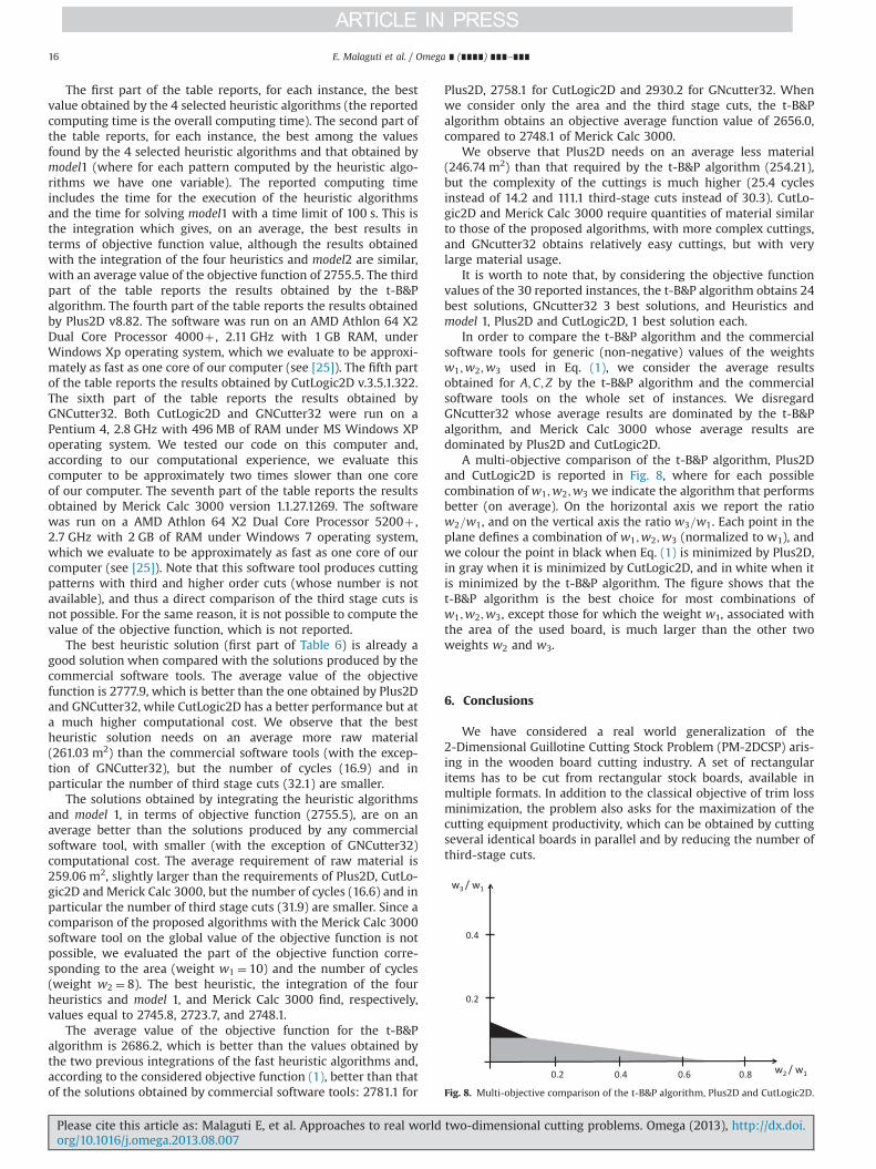
The first part of the table reports, for each instance, the bestvalue obtained by the 4 selected heuristic algorithms (the reportedcomputing time is the overall computing time). The second part ofthe table reports, for each instance, the best among the valuesfound by the 4 selected heuristic algorithms and that obtained bymodel1 (where for each pattern computed by the heuristic algo-rithms we have one variable). The reported computing timeincludes the time for the execution of the heuristic algorithmsand the time for solving model1 with a time limit of 100 s. This isthe integration which gives, on an average, the best results interms of objective function value, although the results obtainedwith the integration of the four heuristics and model2 are similar,with an average value of the objective function of 2755.5. The thirdpart of the table reports the results obtained by the t-B&Palgorithm. The fourth part of the table reports the results obtainedby Plus2D v8.82. The software was run on an AMD Athlon 64 X2Dual Core Processor 4000þ , 2.11 GHz with 1 GB RAM, underWindows Xp operating system, which we evaluate to be approxi-mately as fast as one core of our computer (see [25]). The fifth partof the table reports the results obtained by CutLogic2D v.3.5.1.322.The sixth part of the table reports the results obtained byGNCutter32. Both CutLogic2D and GNCutter32 were run on aPentium 4, 2.8 GHz with 496 MB of RAM under MS Windows XPoperating system. We tested our code on this computer and,according to our computational experience, we evaluate thiscomputer to be approximately two times slower than one coreof our computer. The seventh part of the table reports the resultsobtained by Merick Calc 3000 version 1.1.27.1269. The softwarewas run on a AMD Athlon 64 X2 Dual Core Processor 5200þ ,2.7 GHz with 2 GB of RAM under Windows 7 operating system,which we evaluate to be approximately as fast as one core of ourcomputer (see [25]). Note that this software tool produces cuttingpatterns with third and higher order cuts (whose number is notavailable), and thus a direct comparison of the third stage cuts isnot possible. For the same reason, it is not possible to compute thevalue of the objective function, which is not reported.

The best heuristic solution (first part of Table 6) is already agood solution when compared with the solutions produced by thecommercial software tools. The average value of the objectivefunction is 2777.9, which is better than the one obtained by Plus2Dand GNCutter32, while CutLogic2D has a better performance but ata much higher computational cost. We observe that the bestheuristic solution needs on an average more raw material(261.03 m2) than the commercial software tools (with the excep-tion of GNCutter32), but the number of cycles (16.9) and inparticular the number of third stage cuts (32.1) are smaller.

The solutions obtained by integrating the heuristic algorithmsand model 1, in terms of objective function (2755.5), are on anaverage better than the solutions produced by any commercialsoftware tool, with smaller (with the exception of GNCutter32)computational cost. The average requirement of raw material is259.06 m2, slightly larger than the requirements of Plus2D, CutLo-gic2D and Merick Calc 3000, but the number of cycles (16.6) and inparticular the number of third stage cuts (31.9) are smaller. Since acomparison of the proposed algorithms with the Merick Calc 3000software tool on the global value of the objective function is notpossible, we evaluated the part of the objective function corre-sponding to the area (weight w1 ¼ 10) and the number of cycles(weight w2 ¼ 8). The best heuristic, the integration of the fourheuristics and model 1, and Merick Calc 3000 find, respectively,values equal to 2745.8, 2723.7, and 2748.1.

The average value of the objective function for the t-B&Palgorithm is 2686.2, which is better than the values obtained bythe two previous integrations of the fast heuristic algorithms and,according to the considered objective function (1), better than thatof the solutions obtained by commercial software tools: 2781.1 for

Plus2D, 2758.1 for CutLogic2D and 2930.2 for GNcutter32. Whenwe consider only the area and the third stage cuts, the t-B&Palgorithm obtains an objective average function value of 2656.0,compared to 2748.1 of Merick Calc 3000.

We observe that Plus2D needs on an average less material(246.74 m2) than that required by the t-B&P algorithm (254.21),but the complexity of the cuttings is much higher (25.4 cyclesinstead of 14.2 and 111.1 third-stage cuts instead of 30.3). CutLo-gic2D and Merick Calc 3000 require quantities of material similarto those of the proposed algorithms, with more complex cuttings,and GNcutter32 obtains relatively easy cuttings, but with verylarge material usage.

It is worth to note that, by considering the objective functionvalues of the 30 reported instances, the t-B&P algorithm obtains 24best solutions, GNcutter32 3 best solutions, and Heuristics andmodel 1, Plus2D and CutLogic2D, 1 best solution each.

In order to compare the t-B&P algorithm and the commercialsoftware tools for generic (non-negative) values of the weightsw1;w2;w3 used in Eq. (1), we consider the average resultsobtained for A;C; Z by the t-B&P algorithm and the commercialsoftware tools on the whole set of instances. We disregardGNcutter32 whose average results are dominated by the t-B&Palgorithm, and Merick Calc 3000 whose average results aredominated by Plus2D and CutLogic2D.

A multi-objective comparison of the t-B&P algorithm, Plus2Dand CutLogic2D is reported in Fig. 8, where for each possiblecombination of w1;w2;w3 we indicate the algorithm that performsbetter (on average). On the horizontal axis we report the ratiow2=w1, and on the vertical axis the ratio w3=w1. Each point in theplane defines a combination of w1;w2;w3 (normalized to w1), andwe colour the point in black when Eq. (1) is minimized by Plus2D,in gray when it is minimized by CutLogic2D, and in white when itis minimized by the t-B&P algorithm. The figure shows that thet-B&P algorithm is the best choice for most combinations ofw1;w2;w3, except those for which the weight w1, associated withthe area of the used board, is much larger than the other twoweights w2 and w3.

6. Conclusions

We have considered a real world generalization of the2-Dimensional Guillotine Cutting Stock Problem (PM-2DCSP) aris-ing in the wooden board cutting industry. A set of rectangularitems has to be cut from rectangular stock boards, available inmultiple formats. In addition to the classical objective of trim lossminimization, the problem also asks for the maximization of thecutting equipment productivity, which can be obtained by cuttingseveral identical boards in parallel and by reducing the number ofthird-stage cuts.

Fig. 8. Multi-objective comparison of the t-B&P algorithm, Plus2D and CutLogic2D.







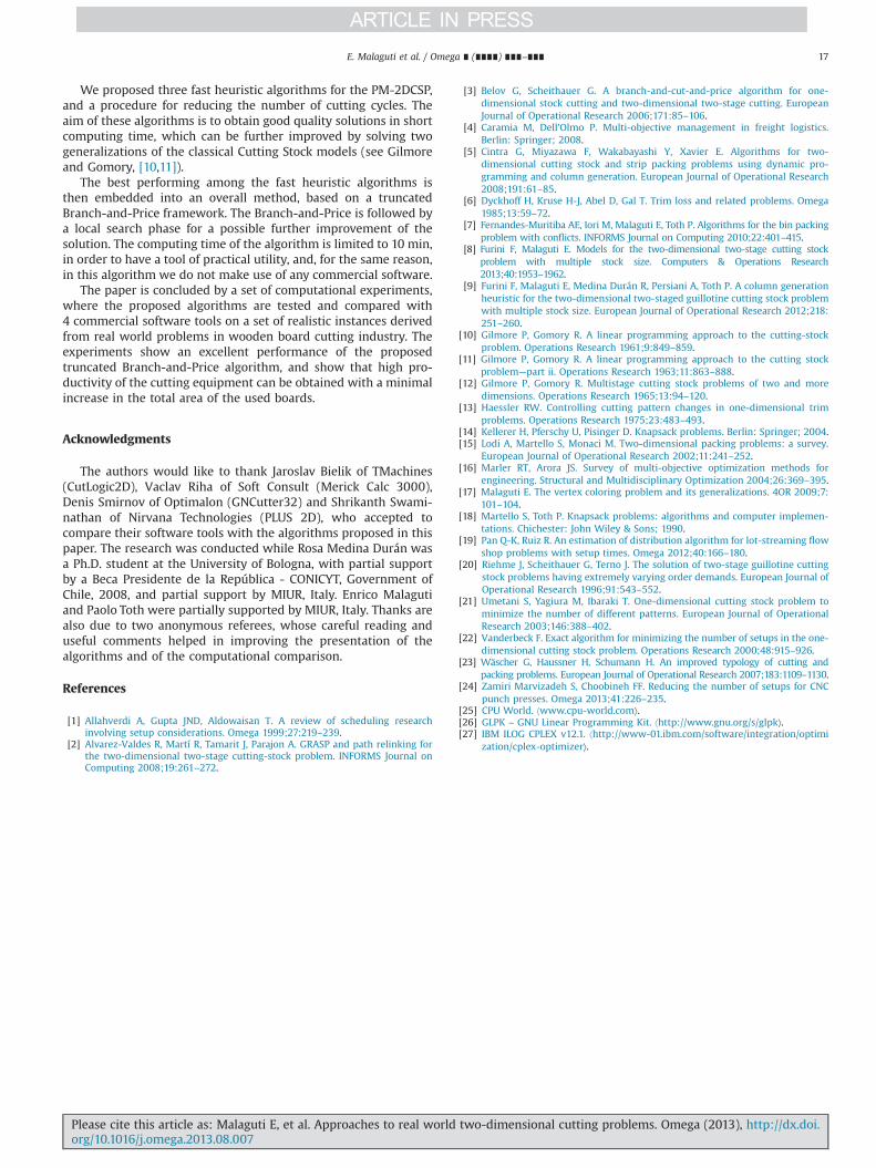
We proposed three fast heuristic algorithms for the PM-2DCSP,and a procedure for reducing the number of cutting cycles. Theaim of these algorithms is to obtain good quality solutions in shortcomputing time, which can be further improved by solving twogeneralizations of the classical Cutting Stock models (see Gilmoreand Gomory, [10,11]).

The best performing among the fast heuristic algorithms isthen embedded into an overall method, based on a truncatedBranch-and-Price framework. The Branch-and-Price is followed bya local search phase for a possible further improvement of thesolution. The computing time of the algorithm is limited to 10 min,in order to have a tool of practical utility, and, for the same reason,in this algorithm we do not make use of any commercial software.

The paper is concluded by a set of computational experiments,where the proposed algorithms are tested and compared with4 commercial software tools on a set of realistic instances derivedfrom real world problems in wooden board cutting industry. Theexperiments show an excellent performance of the proposedtruncated Branch-and-Price algorithm, and show that high pro-ductivity of the cutting equipment can be obtained with a minimalincrease in the total area of the used boards.

Acknowledgments

The authors would like to thank Jaroslav Bielik of TMachines(CutLogic2D), Vaclav Riha of Soft Consult (Merick Calc 3000),Denis Smirnov of Optimalon (GNCutter32) and Shrikanth Swami-nathan of Nirvana Technologies (PLUS 2D), who accepted tocompare their software tools with the algorithms proposed in thispaper. The research was conducted while Rosa Medina Durán wasa Ph.D. student at the University of Bologna, with partial supportby a Beca Presidente de la República - CONICYT, Government ofChile, 2008, and partial support by MIUR, Italy. Enrico Malagutiand Paolo Toth were partially supported by MIUR, Italy. Thanks arealso due to two anonymous referees, whose careful reading anduseful comments helped in improving the presentation of thealgorithms and of the computational comparison.

References

[1] Allahverdi A, Gupta JND, Aldowaisan T. A review of scheduling researchinvolving setup considerations. Omega 1999;27:219–239.

[2] Alvarez-Valdes R, Martí R, Tamarit J, Parajon A. GRASP and path relinking forthe two-dimensional two-stage cutting-stock problem. INFORMS Journal onComputing 2008;19:261–272.

[3] Belov G, Scheithauer G. A branch-and-cut-and-price algorithm for one-dimensional stock cutting and two-dimensional two-stage cutting. EuropeanJournal of Operational Research 2006;171:85–106.

[4] Caramia M, Dell'Olmo P. Multi-objective management in freight logistics.Berlin: Springer; 2008.

[5] Cintra G, Miyazawa F, Wakabayashi Y, Xavier E. Algorithms for two-dimensional cutting stock and strip packing problems using dynamic pro-gramming and column generation. European Journal of Operational Research2008;191:61–85.

[6] Dyckhoff H, Kruse H-J, Abel D, Gal T. Trim loss and related problems. Omega1985;13:59–72.

[7] Fernandes-Muritiba AE, Iori M, Malaguti E, Toth P. Algorithms for the bin packingproblem with conflicts. INFORMS Journal on Computing 2010;22:401–415.

[8] Furini F, Malaguti E. Models for the two-dimensional two-stage cutting stockproblem with multiple stock size. Computers & Operations Research2013;40:1953–1962.

[9] Furini F, Malaguti E, Medina Durán R, Persiani A, Toth P. A column generationheuristic for the two-dimensional two-staged guillotine cutting stock problemwith multiple stock size. European Journal of Operational Research 2012;218:251–260.

[10] Gilmore P, Gomory R. A linear programming approach to the cutting-stockproblem. Operations Research 1961;9:849–859.

[11] Gilmore P, Gomory R. A linear programming approach to the cutting stockproblem—part ii. Operations Research 1963;11:863–888.

[12] Gilmore P, Gomory R. Multistage cutting stock problems of two and moredimensions. Operations Research 1965;13:94–120.

[13] Haessler RW. Controlling cutting pattern changes in one-dimensional trimproblems. Operations Research 1975;23:483–493.

[14] Kellerer H, Pferschy U, Pisinger D. Knapsack problems. Berlin: Springer; 2004.[15] Lodi A, Martello S, Monaci M. Two-dimensional packing problems: a survey.

European Journal of Operational Research 2002;11:241–252.[16] Marler RT, Arora JS. Survey of multi-objective optimization methods for

engineering. Structural and Multidisciplinary Optimization 2004;26:369–395.[17] Malaguti E. The vertex coloring problem and its generalizations. 4OR 2009;7:

101–104.[18] Martello S, Toth P. Knapsack problems: algorithms and computer implemen-

tations. Chichester: John Wiley & Sons; 1990.[19] Pan Q-K, Ruiz R. An estimation of distribution algorithm for lot-streaming flow

shop problems with setup times. Omega 2012;40:166–180.[20] Riehme J, Scheithauer G, Terno J. The solution of two-stage guillotine cutting

stock problems having extremely varying order demands. European Journal ofOperational Research 1996;91:543–552.

[21] Umetani S, Yagiura M, Ibaraki T. One-dimensional cutting stock problem tominimize the number of different patterns. European Journal of OperationalResearch 2003;146:388–402.

[22] Vanderbeck F. Exact algorithm for minimizing the number of setups in the one-dimensional cutting stock problem. Operations Research 2000;48:915–926.

[23] Wäscher G, Haussner H, Schumann H. An improved typology of cutting andpacking problems. European Journal of Operational Research 2007;183:1109–1130.

[24] Zamiri Marvizadeh S, Choobineh FF. Reducing the number of setups for CNCpunch presses. Omega 2013;41:226–235.

[25] CPU World. ⟨www.cpu-world.com⟩.[26] GLPK – GNU Linear Programming Kit. ⟨http://www.gnu.org/s/glpk⟩.[27] IBM ILOG CPLEX v12.1. ⟨http://www-01.ibm.com/software/integration/optimi

zation/cplex-optimizer⟩.



http://refhub.elsevier.com/S0305-0483(13)00091-1/sbref1


























































www.cpu-world.com

http://www.gnu.org/s/glpk

http://www-01.ibm.com/software/integration/optimization/cplex-optimizer

http://www-01.ibm.com/software/integration/optimization/cplex-optimizer





Download - Approaches to real world two-dimensional cutting problems

Top Related