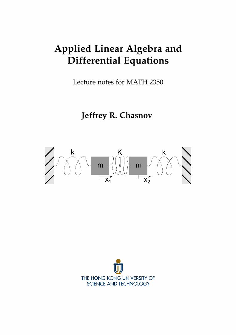
Applied Linear Algebra andDifferential Equations
Lecture notes for MATH 2350
Jeffrey R. Chasnov

The Hong Kong University of Science and TechnologyDepartment of MathematicsClear Water Bay, Kowloon
Hong Kong
Copyright c○ 2017-2019 by Jeffrey Robert Chasnov
This work is licensed under the Creative Commons Attribution 3.0 Hong Kong License. Toview a copy of this license, visit http://creativecommons.org/licenses/by/3.0/hk/ or senda letter to Creative Commons, 171 Second Street, Suite 300, San Francisco, California, 94105,USA.
PrefaceWhat follows are my lecture notes for a mathematics course offered to second-yearengineering students at the the Hong Kong University of Science and Technology.Material from our usual courses on linear algebra and differential equations havebeen combined into a single course (essentially, two half-semester courses) at therequest of our Engineering School. I have tried my best to select the most essentialand interesting topics from both courses, and to show how knowledge of linearalgebra can improve students’ understanding of differential equations.
All web surfers are welcome to download these notes and to use the notes andvideos freely for teaching and learning.
I also have some online courses on Coursera. You can click on the links below toexplore these courses.
If you want to learn differential equations, have a look at
Differential Equations for Engineers
If your interests are matrices and elementary linear algebra, try
Matrix Algebra for Engineers
If you want to learn vector calculus (also known as multivariable calculus, or calcu-lus three), you can sign up for
Vector Calculus for Engineers
And if you simply want to enjoy mathematics, my very first online course is stillavailable:
Fibonacci Numbers and the Golden Ratio
Jeffrey R. Chasnov
Hong KongJanuary 2020
iii

Contents0 A short mathematical review 1
0.1 The trigonometric functions . . . . . . . . . . . . . . . . . . . . . . . . . 10.2 The exponential function and the natural logarithm . . . . . . . . . . . 10.3 Definition of the derivative . . . . . . . . . . . . . . . . . . . . . . . . . 20.4 Differentiating a combination of functions . . . . . . . . . . . . . . . . 2
0.4.1 The sum or difference rule . . . . . . . . . . . . . . . . . . . . . 20.4.2 The product rule . . . . . . . . . . . . . . . . . . . . . . . . . . . 20.4.3 The quotient rule . . . . . . . . . . . . . . . . . . . . . . . . . . . 20.4.4 The chain rule . . . . . . . . . . . . . . . . . . . . . . . . . . . . . 2
0.5 Differentiating elementary functions . . . . . . . . . . . . . . . . . . . . 30.5.1 The power rule . . . . . . . . . . . . . . . . . . . . . . . . . . . . 30.5.2 Trigonometric functions . . . . . . . . . . . . . . . . . . . . . . . 30.5.3 Exponential and natural logarithm functions . . . . . . . . . . . 3
0.6 Definition of the integral . . . . . . . . . . . . . . . . . . . . . . . . . . . 30.7 The fundamental theorem of calculus . . . . . . . . . . . . . . . . . . . 40.8 Definite and indefinite integrals . . . . . . . . . . . . . . . . . . . . . . . 50.9 Indefinite integrals of elementary functions . . . . . . . . . . . . . . . . 50.10 Substitution . . . . . . . . . . . . . . . . . . . . . . . . . . . . . . . . . . 60.11 Integration by parts . . . . . . . . . . . . . . . . . . . . . . . . . . . . . . 60.12 Taylor series . . . . . . . . . . . . . . . . . . . . . . . . . . . . . . . . . . 60.13 Functions of several variables . . . . . . . . . . . . . . . . . . . . . . . . 70.14 Complex numbers . . . . . . . . . . . . . . . . . . . . . . . . . . . . . . 8
I Linear algebra 13
1 Matrices 171.1 Definition of a matrix . . . . . . . . . . . . . . . . . . . . . . . . . . . . . 171.2 Addition and multiplication of matrices . . . . . . . . . . . . . . . . . . 171.3 The identity matrix and the zero matrix . . . . . . . . . . . . . . . . . . 191.4 General notation, transposes, and inverses . . . . . . . . . . . . . . . . 191.5 Rotation matrices and orthogonal matrices . . . . . . . . . . . . . . . . 231.6 Matrix representation of complex numbers . . . . . . . . . . . . . . . . 241.7 Permutation matrices . . . . . . . . . . . . . . . . . . . . . . . . . . . . . 251.8 Projection matrices . . . . . . . . . . . . . . . . . . . . . . . . . . . . . . 26
2 Systems of linear equations 272.1 Gaussian Elimination . . . . . . . . . . . . . . . . . . . . . . . . . . . . . 272.2 When there is no unique solution . . . . . . . . . . . . . . . . . . . . . . 282.3 Reduced row echelon form . . . . . . . . . . . . . . . . . . . . . . . . . 292.4 Computing inverses . . . . . . . . . . . . . . . . . . . . . . . . . . . . . 302.5 LU decomposition . . . . . . . . . . . . . . . . . . . . . . . . . . . . . . 31
v
CONTENTS
3 Vector spaces 353.1 Vector spaces . . . . . . . . . . . . . . . . . . . . . . . . . . . . . . . . . 353.2 Linear independence . . . . . . . . . . . . . . . . . . . . . . . . . . . . . 373.3 Span, basis and dimension . . . . . . . . . . . . . . . . . . . . . . . . . . 373.4 Inner product spaces . . . . . . . . . . . . . . . . . . . . . . . . . . . . . 393.5 Vector spaces of a matrix . . . . . . . . . . . . . . . . . . . . . . . . . . . 40
3.5.1 Null space . . . . . . . . . . . . . . . . . . . . . . . . . . . . . . . 403.5.2 Application of the null space . . . . . . . . . . . . . . . . . . . . 413.5.3 Column space . . . . . . . . . . . . . . . . . . . . . . . . . . . . . 423.5.4 Row space, left null space and rank . . . . . . . . . . . . . . . . 43
3.6 Gram-Schmidt process . . . . . . . . . . . . . . . . . . . . . . . . . . . . 443.7 Orthogonal projections . . . . . . . . . . . . . . . . . . . . . . . . . . . . 453.8 QR factorization . . . . . . . . . . . . . . . . . . . . . . . . . . . . . . . . 463.9 The least-squares problem . . . . . . . . . . . . . . . . . . . . . . . . . . 473.10 Solution of the least-squares problem . . . . . . . . . . . . . . . . . . . 49
4 Determinants 514.1 Two-by-two and three-by-three determinants . . . . . . . . . . . . . . . 514.2 Laplace expansion and Leibniz formula . . . . . . . . . . . . . . . . . . 524.3 Properties of the determinant . . . . . . . . . . . . . . . . . . . . . . . . 534.4 Use of determinants in Vector Calculus . . . . . . . . . . . . . . . . . . 58
5 Eigenvalues and eigenvectors 635.1 The eigenvalue problem . . . . . . . . . . . . . . . . . . . . . . . . . . . 635.2 Matrix diagonalization . . . . . . . . . . . . . . . . . . . . . . . . . . . . 665.3 Symmetric and Hermitian matrices . . . . . . . . . . . . . . . . . . . . . 68
II Differential equations 69
6 Introduction to odes 736.1 The simplest type of differential equation . . . . . . . . . . . . . . . . . 73
7 First-order odes 757.1 The Euler method . . . . . . . . . . . . . . . . . . . . . . . . . . . . . . . 757.2 Separable equations . . . . . . . . . . . . . . . . . . . . . . . . . . . . . 767.3 Linear equations . . . . . . . . . . . . . . . . . . . . . . . . . . . . . . . 797.4 Applications . . . . . . . . . . . . . . . . . . . . . . . . . . . . . . . . . . 82
7.4.1 Compound interest . . . . . . . . . . . . . . . . . . . . . . . . . . 827.4.2 Chemical reactions . . . . . . . . . . . . . . . . . . . . . . . . . . 837.4.3 Terminal velocity . . . . . . . . . . . . . . . . . . . . . . . . . . . 857.4.4 Escape velocity . . . . . . . . . . . . . . . . . . . . . . . . . . . . 867.4.5 RC circuit . . . . . . . . . . . . . . . . . . . . . . . . . . . . . . . 877.4.6 The logistic equation . . . . . . . . . . . . . . . . . . . . . . . . . 89
8 Second-order odes, constant coefficients 918.1 The Euler method . . . . . . . . . . . . . . . . . . . . . . . . . . . . . . . 918.2 The principle of superposition . . . . . . . . . . . . . . . . . . . . . . . 928.3 The Wronskian . . . . . . . . . . . . . . . . . . . . . . . . . . . . . . . . 928.4 Homogeneous odes . . . . . . . . . . . . . . . . . . . . . . . . . . . . . . 93
8.4.1 Distinct real roots . . . . . . . . . . . . . . . . . . . . . . . . . . . 948.4.2 Distinct complex-conjugate roots . . . . . . . . . . . . . . . . . . 96
vi CONTENTS
CONTENTS
8.4.3 Degenerate roots . . . . . . . . . . . . . . . . . . . . . . . . . . . 988.5 Difference equations . . . . . . . . . . . . . . . . . . . . . . . . . . . . . 998.6 Inhomogeneous odes . . . . . . . . . . . . . . . . . . . . . . . . . . . . . 1008.7 Resonance . . . . . . . . . . . . . . . . . . . . . . . . . . . . . . . . . . . 1048.8 Applications . . . . . . . . . . . . . . . . . . . . . . . . . . . . . . . . . . 107
8.8.1 RLC circuit . . . . . . . . . . . . . . . . . . . . . . . . . . . . . . 1078.8.2 Mass on a spring . . . . . . . . . . . . . . . . . . . . . . . . . . . 1098.8.3 Pendulum . . . . . . . . . . . . . . . . . . . . . . . . . . . . . . . 110
8.9 Damped resonance . . . . . . . . . . . . . . . . . . . . . . . . . . . . . . 111
9 Series solutions 1139.1 Ordinary points . . . . . . . . . . . . . . . . . . . . . . . . . . . . . . . . 113
10 Systems of linear differential equations 11910.1 Distinct real eigenvalues . . . . . . . . . . . . . . . . . . . . . . . . . . . 11910.2 Solution by diagonalization . . . . . . . . . . . . . . . . . . . . . . . . . 12110.3 Solution by the matrix exponential . . . . . . . . . . . . . . . . . . . . . 12210.4 Distinct complex-conjugate eigenvalues . . . . . . . . . . . . . . . . . . 12310.5 Repeated eigenvalues with one eigenvector . . . . . . . . . . . . . . . . 12510.6 Normal modes . . . . . . . . . . . . . . . . . . . . . . . . . . . . . . . . . 127
11 Nonlinear differential equations 13111.1 Fixed points and stability . . . . . . . . . . . . . . . . . . . . . . . . . . 131
11.1.1 One dimension . . . . . . . . . . . . . . . . . . . . . . . . . . . . 13111.1.2 Two dimensions . . . . . . . . . . . . . . . . . . . . . . . . . . . 132
11.2 Bifurcation theory . . . . . . . . . . . . . . . . . . . . . . . . . . . . . . . 13411.2.1 Saddle-node bifurcation . . . . . . . . . . . . . . . . . . . . . . . 13511.2.2 Transcritical bifurcation . . . . . . . . . . . . . . . . . . . . . . . 13611.2.3 Supercritical pitchfork bifurcation . . . . . . . . . . . . . . . . . 13711.2.4 Subcritical pitchfork bifurcation . . . . . . . . . . . . . . . . . . 13711.2.5 Application: a mathematical model of a fishery . . . . . . . . . 140
CONTENTS vii

CONTENTS
viii CONTENTS
Chapter 0
A short mathematical reviewA basic understanding of pre-calculus, calculus, and complex numbers is re-
quired for this course. This zero chapter presents a concise review.
0.1 The trigonometric functions
The Pythagorean trigonometric identity is
sin2 x + cos2 x = 1,
and the addition theorems are
sin(x + y) = sin(x) cos(y) + cos(x) sin(y),cos(x + y) = cos(x) cos(y)− sin(x) sin(y).
Also, the values of sin x in the first quadrant can be remembered by the rule ofquarters, with 0◦ = 0, 30◦ = π/6, 45◦ = π/4, 60◦ = π/3, 90◦ = π/2:
sin 0◦ =
√04
, sin 30◦ =
√14
, sin 45◦ =
√24
,
sin 60◦ =
√34
, sin 90◦ =
√44
.
The following symmetry properties are also useful:
sin(π/2− x) = cos x, cos(π/2− x) = sin x;
andsin(−x) = − sin(x), cos(−x) = cos(x).
0.2 The exponential function and the natural logarithm
The transcendental number e, approximately 2.71828, is defined as
e = limn→∞
(1 +
1n
)n.
The exponential function exp (x) = ex and natural logarithm ln x are inverse func-tions satisfying
eln x = x, ln ex = x.
The usual rules of exponents apply:
exey = ex+y, ex/ey = ex−y, (ex)p = epx.
The corresponding rules for the logarithmic function are
ln (xy) = ln x + ln y, ln (x/y) = ln x− ln y, ln xp = p ln x.
1

0.3. DEFINITION OF THE DERIVATIVE
0.3 Definition of the derivative
The derivative of the function y = f (x), denoted as f ′(x) or dy/dx, is defined asthe slope of the tangent line to the curve y = f (x) at the point (x, y). This slope isobtained by a limit, and is defined as
f ′(x) = limh→0
f (x + h)− f (x)h
. (1)
0.4 Differentiating a combination of functions
0.4.1 The sum or difference rule
The derivative of the sum of f (x) and g(x) is
( f + g)′ = f ′ + g′.
Similarly, the derivative of the difference is
( f − g)′ = f ′ − g′.
0.4.2 The product rule
The derivative of the product of f (x) and g(x) is
( f g)′ = f ′g + f g′,
and should be memorized as “the derivative of the first times the second plus thefirst times the derivative of the second.”
0.4.3 The quotient rule
The derivative of the quotient of f (x) and g(x) is(fg
)′=
f ′g− f g′
g2 ,
and should be memorized as “the derivative of the top times the bottom minus thetop times the derivative of the bottom over the bottom squared.”
0.4.4 The chain rule
The derivative of the composition of f (x) and g(x) is(f(
g(x)))′
= f ′(
g(x))· g′(x),
and should be memorized as “the derivative of the outside times the derivative ofthe inside.”
2 CHAPTER 0. A SHORT MATHEMATICAL REVIEW
0.5. DIFFERENTIATING ELEMENTARY FUNCTIONS
0.5 Differentiating elementary functions
0.5.1 The power ruleThe derivative of a power of x is given by
ddx
xp = pxp−1.
0.5.2 Trigonometric functionsThe derivatives of sin x and cos x are
(sin x)′ = cos x, (cos x)′ = − sin x.
We thus say that “the derivative of sine is cosine,” and “the derivative of cosine isminus sine.” Notice that the second derivatives satisfy
(sin x)′′ = − sin x, (cos x)′′ = − cos x.
0.5.3 Exponential and natural logarithm functionsThe derivative of ex and ln x are
(ex)′ = ex, (ln x)′ =1x
.
0.6 Definition of the integral
The definite integral of a function f (x) > 0 from x = a to b (b > a) is definedas the area bounded by the vertical lines x = a, x = b, the x-axis and the curvey = f (x). This “area under the curve” is obtained by a limit. First, the area isapproximated by a sum of rectangle areas. Second, the integral is defined to be thelimit of the rectangle areas as the width of each individual rectangle goes to zeroand the number of rectangles goes to infinity. This resulting infinite sum is called aRiemann Sum, and we define
∫ b
af (x)dx = lim
h→0
N
∑n=1
f(a + (n− 1)h
)· h, (2)
where N = (b− a)/h is the number of terms in the sum. The symbols on the left-hand-side of (2) are read as “the integral from a to b of f of x dee x.” The RiemannSum definition is extended to all values of a and b and for all values of f (x) (positiveand negative). Accordingly,∫ a
bf (x)dx = −
∫ b
af (x)dx and
∫ b
a(− f (x))dx = −
∫ b
af (x)dx.
Also, ∫ c
af (x)dx =
∫ b
af (x)dx +
∫ c
bf (x)dx,
which states when f (x) > 0 and a < b < c that the total area is equal to the sum ofits parts.
CHAPTER 0. A SHORT MATHEMATICAL REVIEW 3

0.7. THE FUNDAMENTAL THEOREM OF CALCULUS
0.7 The fundamental theorem of calculus
View tutorial on YouTube
Using the definition of the derivative, we differentiate the following integral:
ddx
∫ x
af (s)ds = lim
h→0
∫ x+ha f (s)ds−
∫ xa f (s)ds
h
= limh→0
∫ x+hx f (s)ds
h
= limh→0
h f (x)h
= f (x).
This result is called the fundamental theorem of calculus, and provides a connectionbetween differentiation and integration.
The fundamental theorem teaches us how to integrate functions. Let F(x) be afunction such that F′(x) = f (x). We say that F(x) is an antiderivative of f (x). Thenfrom the fundamental theorem and the fact that the derivative of a constant equalszero,
F(x) =∫ x
af (s)ds + c.
Now, F(a) = c and F(b) =∫ b
a f (s)ds + F(a). Therefore, the fundamental theoremshows us how to integrate a function f (x) provided we can find its antiderivative:
∫ b
af (s)ds = F(b)− F(a). (3)
Unfortunately, finding antiderivatives is much harder than finding derivatives, andindeed, most complicated functions cannot be integrated analytically.
We can also derive the very important result (3) directly from the definition ofthe derivative (1) and the definite integral (2). We will see it is convenient to choosethe same h in both limits. With F′(x) = f (x), we have
∫ b
af (s)ds =
∫ b
aF′(s)ds
= limh→0
N
∑n=1
F′(a + (n− 1)h
)· h
= limh→0
N
∑n=1
F(a + nh)− F(a + (n− 1)h
)h
· h
= limh→0
N
∑n=1
F(a + nh)− F(a + (n− 1)h
).
The last expression has an interesting structure. All the values of F(x) evaluatedat the points lying between the endpoints a and b cancel each other in consecutiveterms. Only the value −F(a) survives when n = 1, and the value +F(b) whenn = N, yielding again (3).
4 CHAPTER 0. A SHORT MATHEMATICAL REVIEW
0.8. DEFINITE AND INDEFINITE INTEGRALS
0.8 Definite and indefinite integrals
The Riemann sum definition of an integral is called a definite integral. It is convenientto also define an indefinite integral by∫
f (x)dx = F(x),
where F(x) is the antiderivative of f (x).
0.9 Indefinite integrals of elementary functions
From our known derivatives of elementary functions, we can determine some sim-ple indefinite integrals. The power rule gives us∫
xndx =xn+1
n + 1+ c, n 6= −1.
When n = −1, and x is positive, we have∫ 1x
dx = ln x + c.
If x is negative, using the chain rule we have
ddx
ln (−x) =1x
.
Therefore, since
|x| ={−x if x < 0;x if x > 0,
we can generalize our indefinite integral to strictly positive or strictly negative x:∫ 1x
dx = ln |x|+ c.
Trigonometric functions can also be integrated:∫cos xdx = sin x + c,
∫sin xdx = − cos x + c.
Easily proved identities are an addition rule:∫ (f (x) + g(x)
)dx =
∫f (x)dx +
∫g(x)dx;
and multiplication by a constant:∫A f (x)dx = A
∫f (x)dx.
This permits integration of functions such as∫(x2 + 7x + 2)dx =
x3
3+
7x2
2+ 2x + c,
and ∫(5 cos x + sin x)dx = 5 sin x− cos x + c.
CHAPTER 0. A SHORT MATHEMATICAL REVIEW 5
0.10. SUBSTITUTION
0.10 Substitution
More complicated functions can be integrated using the chain rule. Since
ddx
f(
g(x))= f ′
(g(x)
)· g′(x),
we have ∫f ′(
g(x))· g′(x)dx = f
(g(x)
)+ c.
This integration formula is usually implemented by letting y = g(x). Then onewrites dy = g′(x)dx to obtain∫
f ′(
g(x))
g′(x)dx =∫
f ′(y)dy
= f (y) + c
= f(
g(x))+ c.
0.11 Integration by parts
Another integration technique makes use of the product rule for differentiation.Since
( f g)′ = f ′g + f g′,
we havef ′g = ( f g)′ − f g′.
Therefore, ∫f ′(x)g(x)dx = f (x)g(x)−
∫f (x)g′(x)dx.
Commonly, the above integral is done by writing
u = g(x) dv = f ′(x)dxdu = g′(x)dx v = f (x).
Then, the formula to be memorized is∫udv = uv−
∫vdu.
0.12 Taylor series
A Taylor series of a function f (x) about a point x = a is a power series repre-sentation of f (x) developed so that all the derivatives of f (x) at a match all thederivatives of the power series. Without worrying about convergence here, we have
f (x) = f (a) + f ′(a)(x− a) +f ′′(a)
2!(x− a)2 +
f ′′′(a)3!
(x− a)3 + . . . .
Notice that the first term in the power series matches f (a), all other terms vanishing,the second term matches f ′(a), all other terms vanishing, etc. Commonly, the Taylor
6 CHAPTER 0. A SHORT MATHEMATICAL REVIEW
0.13. FUNCTIONS OF SEVERAL VARIABLES
series is developed with a = 0. We will also make use of the Taylor series in aslightly different form, with x = x∗ + ε and a = x∗:
f (x∗ + ε) = f (x∗) + f ′(x∗)ε +f ′′(x∗)
2!ε2 +
f ′′′(x∗)3!
ε3 + . . . .
Another way to view this series is that of g(ε) = f (x∗ + ε), expanded about ε = 0.Taylor series that are commonly used include
ex = 1 + x +x2
2!+
x3
3!+ . . . ,
sin x = x− x3
3!+
x5
5!− . . . ,
cos x = 1− x2
2!+
x4
4!− . . . ,
11 + x
= 1− x + x2 − . . . , for |x| < 1,
ln (1 + x) = x− x2
2+
x3
3− . . . , for |x| < 1.
0.13 Functions of several variables
For simplicity, we consider a function f = f (x, y) of two variables, though theresults are easily generalized. The partial derivative of f with respect to x is definedas
∂ f∂x
= limh→0
f (x + h, y)− f (x, y)h
,
and similarly for the partial derivative of f with respect to y. To take the partialderivative of f with respect to x, say, take the derivative of f with respect to xholding y fixed. As an example, consider
f (x, y) = 2x3y2 + y3.
We have∂ f∂x
= 6x2y2,∂ f∂y
= 4x3y + 3y2.
Second derivatives are defined as the derivatives of the first derivatives, so we have
∂2 f∂x2 = 12xy2,
∂2 f∂y2 = 4x3 + 6y;
and the mixed second partial derivatives are
∂2 f∂x∂y
= 12x2y,∂2 f
∂y∂x= 12x2y.
In general, mixed partial derivatives are independent of the order in which thederivatives are taken.
Partial derivatives are necessary for applying the chain rule. Consider
d f = f (x + dx, y + dy)− f (x, y).
CHAPTER 0. A SHORT MATHEMATICAL REVIEW 7

0.14. COMPLEX NUMBERS
We can write d f as
d f = [ f (x + dx, y + dy)− f (x, y + dy)] + [ f (x, y + dy)− f (x, y)]
=∂ f∂x
dx +∂ f∂y
dy.
If one has f = f (x(t), y(t)), say, then
d fdt
=∂ f∂x
dxdt
+∂ f∂y
dydt
.
And if one has f = f (x(r, θ), y(r, θ)), say, then
∂ f∂r
=∂ f∂x
∂x∂r
+∂ f∂y
∂y∂r
,∂ f∂θ
=∂ f∂x
∂x∂θ
+∂ f∂y
∂y∂θ
.
A Taylor series of a function of several variables can also be developed. Here, allpartial derivatives of f (x, y) at (a, b) match all the partial derivatives of the powerseries. With the notation
fx =∂ f∂x
, fy =∂ f∂y
, fxx =∂2 f∂x2 , fxy =
∂2 f∂x∂y
, fyy =∂2 f∂y2 , etc.,
we have
f (x, y) = f (a, b) + fx(a, b)(x− a) + fy(a, b)(y− b)
+12!
(fxx(a, b)(x− a)2 + 2 fxy(a, b)(x− a)(y− b) + fyy(a, b)(y− b)2
)+ . . .
0.14 Complex numbers
View tutorial on YouTube: Complex NumbersView tutorial on YouTube: Complex Exponential Function
We define the imaginary number i to be one of the two numbers that satisfies therule (i)2 = −1, the other number being −i. Formally, we write i =
√−1. A complex
number z is written asz = x + iy,
where x and y are real numbers. We call x the real part of z and y the imaginarypart and write
x = Re z, y = Im z.
Two complex numbers are equal if and only if their real and imaginary parts areequal.
The complex conjugate of z = x + iy, denoted as z, is defined as
z = x− iy.
Using z and z, we have
Re z =12(z + z) , Im z =
12i
(z− z) . (4)
8 CHAPTER 0. A SHORT MATHEMATICAL REVIEW
0.14. COMPLEX NUMBERS
Furthermore,
zz = (x + iy)(x− iy)
= x2 − i2y2
= x2 + y2;
and we define the absolute value of z, also called the modulus of z, by
|z| = (zz)1/2
=√
x2 + y2.
We can add, subtract, multiply and divide complex numbers to get new complexnumbers. With z = x + iy and w = s + it, and x, y, s, t real numbers, we have
z + w = (x + s) + i(y + t); z− w = (x− s) + i(y− t);
zw = (x + iy)(s + it)= (xs− yt) + i(xt + ys);
zw
=zwww
=(x + iy)(s− it)
s2 + t2
=(xs + yt)
s2 + t2 + i(ys− xt)
s2 + t2 .
Furthermore,
|zw| =√(xs− yt)2 + (xt + ys)2
=√(x2 + y2)(s2 + t2)
= |z||w|;and
zw = (xs− yt)− i(xt + ys)= (x− iy)(s− it)= zw.
Similarly ∣∣∣ zw
∣∣∣ = |z||w| , (zw) =
zw
.
Also, z + w = z + w. However, |z + w| ≤ |z|+ |w|, a theorem known as the triangleinequality.
It is especially interesting and useful to consider the exponential function of animaginary argument. Using the Taylor series expansion of an exponential function,we have
eiθ = 1 + (iθ) +(iθ)2
2!+
(iθ)3
3!+
(iθ)4
4!+
(iθ)5
5!. . .
=
(1− θ2
2!+
θ4
4!− . . .
)+ i(
θ − θ3
3!+
θ5
5!+ . . .
)= cos θ + i sin θ.
CHAPTER 0. A SHORT MATHEMATICAL REVIEW 9
0.14. COMPLEX NUMBERS
Since we have determined that
cos θ = Re eiθ , sin θ = Im eiθ , (5)
we also have using (4) and (5), the frequently used expressions
cos θ =eiθ + e−iθ
2, sin θ =
eiθ − e−iθ
2i.
The much celebrated Euler’s identity derives from eiθ = cos θ + i sin θ by settingθ = π, and using cos π = −1 and sin π = 0:
eiπ + 1 = 0,
and this identity links the five fundamental numbers—0, 1, i, e and π—using threebasic mathematical operations—addition, multiplication and exponentiation—onlyonce.
z=x+iy
θ
r
x
Re(z)
y
Im(z
)
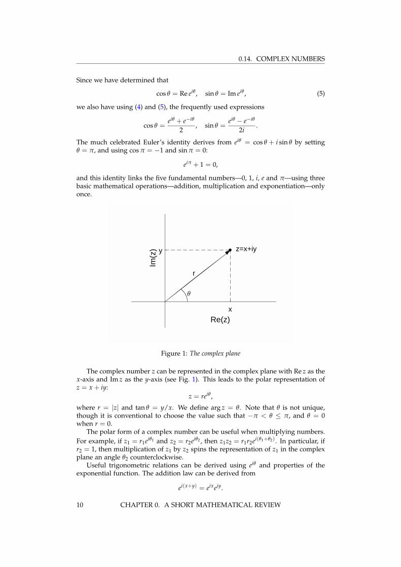
Figure 1: The complex plane
The complex number z can be represented in the complex plane with Re z as thex-axis and Im z as the y-axis (see Fig. 1). This leads to the polar representation ofz = x + iy:
z = reiθ ,
where r = |z| and tan θ = y/x. We define arg z = θ. Note that θ is not unique,though it is conventional to choose the value such that −π < θ ≤ π, and θ = 0when r = 0.
The polar form of a complex number can be useful when multiplying numbers.For example, if z1 = r1eiθ1 and z2 = r2eiθ2 , then z1z2 = r1r2ei(θ1+θ2). In particular, ifr2 = 1, then multiplication of z1 by z2 spins the representation of z1 in the complexplane an angle θ2 counterclockwise.
Useful trigonometric relations can be derived using eiθ and properties of theexponential function. The addition law can be derived from
ei(x+y) = eixeiy.
10 CHAPTER 0. A SHORT MATHEMATICAL REVIEW

0.14. COMPLEX NUMBERS
We have
cos(x + y) + i sin(x + y) = (cos x + i sin x)(cos y + i sin y)= (cos x cos y− sin x sin y) + i(sin x cos y + cos x sin y);
yielding
cos(x + y) = cos x cos y− sin x sin y, sin(x + y) = sin x cos y + cos x sin y.
De Moivre’s Theorem derives from einθ = (eiθ)n, yielding the identity
cos(nθ) + i sin(nθ) = (cos θ + i sin θ)n.
For example, if n = 2, we derive
cos 2θ + i sin 2θ = (cos θ + i sin θ)2
= (cos2 θ − sin2 θ) + 2i cos θ sin θ.
Therefore,cos 2θ = cos2 θ − sin2 θ, sin 2θ = 2 cos θ sin θ.
Example: Write√
i as a standard complex number
To solve this example, we first need to define what is meant by the square rootof a complex number. The meaning of
√z is the complex number whose square
is z. There will always be two such numbers, because (√
z)2 = (−√
z)2 = z. Onecan not define the positive square root because complex numbers are not definedas positive or negative.
We will show two methods to solve this problem. The first most straightforwardmethod writes √
i = x + iy.
Squaring both sides, we obtain
i = x2 − y2 + 2xyi;
and equating the real and imaginary parts of this equation yields the two real equa-tions
x2 − y2 = 0, 2xy = 1.
The first equation yields y = ±x. With y = x, the second equation yields 2x2 = 1with two solutions x = ±
√2/2. With y = −x, the second equation yields −2x2 = 1,
which has no solution for real x. We have therefore found that
√i = ±
(√2
2+ i√
22
).
The second solution method makes use of the polar form of complex numbers.The algebra required for this method is somewhat simpler, especially for findingcube roots, fourth roots, etc. We know that i = eiπ/2, but more generally because ofthe periodic nature of the polar angle, we can write
i = ei( π2 +2πk),
CHAPTER 0. A SHORT MATHEMATICAL REVIEW 11
0.14. COMPLEX NUMBERS
where k is an integer. We then have√
i = i1/2 = ei( π4 +πk) = eiπkeiπ/4 = ±eiπ/4,
where we have made use of the usual properties of the exponential function, andeiπk = ±1 for k even or odd. Converting back to standard form, we have
√i = ± (cos π/4 + i sin π/4) = ±
(√2
2+ i√
22
).
The fundamental theorem of algebra states that every polynomial equation ofdegree n has exactly n complex roots, counted with multiplicity. Two familiar ex-amples would be x2 − 1 = (x + 1)(x− 1) = 0, with two roots x1 = −1 and x2 = 1;and x2 − 2x + 1 = (x− 1)2 = 0, with one root x1 = 1 with multiplicity two.
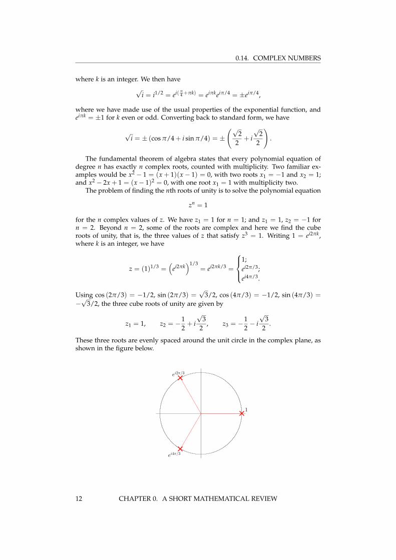
The problem of finding the nth roots of unity is to solve the polynomial equation
zn = 1
for the n complex values of z. We have z1 = 1 for n = 1; and z1 = 1, z2 = −1 forn = 2. Beyond n = 2, some of the roots are complex and here we find the cuberoots of unity, that is, the three values of z that satisfy z3 = 1. Writing 1 = ei2πk,where k is an integer, we have
z = (1)1/3 =(
ei2πk)1/3
= ei2πk/3 =
1;ei2π/3;ei4π/3.
Using cos (2π/3) = −1/2, sin (2π/3) =√
3/2, cos (4π/3) = −1/2, sin (4π/3) =−√
3/2, the three cube roots of unity are given by
z1 = 1, z2 = −12+ i√
32
, z3 = −12− i√
32
.
These three roots are evenly spaced around the unit circle in the complex plane, asshown in the figure below.
ei2π/3
ei4π/3
1
12 CHAPTER 0. A SHORT MATHEMATICAL REVIEW
Part I
Linear algebra
13


The first part of this course is on linear algebra. We begin by introducing matri-ces and matrix algebra. Next, the important algorithm of Gaussian elimination andLU-decomposition is presented and used to solve a system of linear equations andinvert a matrix. We then discuss the abstract concept of vector and inner productspaces, and show how these concepts are related to matrices. Finally, a thoroughpresentation of determinants is given and the determinant is then used to solve thevery important eigenvalue problem.
15

16
Chapter 1
Matrices1.1 Definition of a matrix
View Definition of a Matrix on YouTube
An m-by-n matrix is a rectangular array of numbers (or other mathematical ob-jects) with m rows and n columns. For example, a two-by-two matrix A, with tworows and two columns, looks like
A =
(a bc d
).
(Sometimes brackets are used instead of parentheses.) The first row has elements aand b, the second row has elements c and d. The first column has elements a andc; the second column has elements b and d. As further examples, 2-by-3 and 3-by-2matrices look like
B =
(a b cd e f
), C =
a bc de f
.
Of special importance are the so-called row matrices and column matrices. Thesematrices are also called row vectors and column vectors. The row vector is ingeneral 1-by-n and the column vector is n-by-1. For example, when n = 3, wewould write
v =(a b c
)as a row vector, and
v =
abc
as a column vector.
1.2 Addition and multiplication of matrices
View Addition & Multiplication of Matrices on YouTube
Matrices can be added and multiplied. Matrices can be added only if they havethe same dimension, and addition proceeds element by element. For example,(
a bc d
)+
(e fg h
)=
(a + e b + fc + g d + h
).
Multiplication of a matrix by a scalar is also easy. The rule is to just multiply everyelement of the matrix by the scalar. The 2-by-2 case is illustrated as
k(
a bc d
)=
(ka kbkc kd
).
17
1.2. ADDITION AND MULTIPLICATION OF MATRICES
Matrix multiplication, however, is more complicated. Matrices (excluding the scalar)can be multiplied only if the number of columns of the left matrix equals the num-ber of rows of the right matrix. In other words, an m-by-n matrix on the left can bemultiplied by an n-by-k matrix on the right. The resulting matrix will be m-by-k.We can illustrate matrix multiplication using two 2-by-2 matrices, writing(
a bc d
)(e fg h
)=
(ae + bg a f + bhce + dg c f + dh
).
The standard way to multiply matrices is as follows. The first row of the left matrixis multiplied against and summed with the first column of the right matrix to obtainthe element in the first row and first column of the product matrix. Next, the firstrow is multiplied against and summed with the second column; then the secondrow is multiplied against and summed with the first column; and finally the secondrow is multiplied against and summed with the second column.
In general, a particular element in the resulting product matrix, say in row k andcolumn l, is obtained by multiplying and summing the elements in row k of the leftmatrix with the elements in column l of the right matrix.
Example: Consider the Fibonacci Q-matrix given by
Q =
(1 11 0
)Determine Qn in terms of the Fibonacci numbers.
The famous Fibonacci sequence is 1, 1, 2, 3, 5, 8, 13, . . . , where each number in thesequence is the sum of the preceeding two numbers, and the first two numbers areset equal to one. With Fn the nth Fibonacci number, the mathematical definition is
Fn+1 = Fn + Fn−1, F1 = F2 = 1,
and we may define F0 = 0 so that F0 + F1 = F2.Notice what happens when a matrix is multiplied by Q on the left:(
1 11 0
)(a bc d
)=
(a + c b + d
a c
).
The first row is replaced by the sum of the first and second rows, and the secondrow is replaced by the first row. Using the Fibonacci numbers, we can cleverly writethe Fibonacci Q-matrix as
Q =
(1 11 0
)=
(F2 F1F1 F0
);
and then using the Fibonacci recursion relation we have
Q2 =
(F3 F2F2 F1
), Q3 =
(F4 F3F3 F2
).
More generally,
Qn =
(Fn+1 Fn
Fn Fn−1
).
18 CHAPTER 1. MATRICES
1.3. THE IDENTITY MATRIX AND THE ZERO MATRIX
1.3 The identity matrix and the zero matrix
View Special Matrices on YouTube
Two special matrices are the identity matrix, denoted by I, and the zero matrix,denoted simply by 0. The zero matrix can be m-by-n and is a matrix consisting ofall zero elements. The identity matrix is a square matrix. If A and I are of the samesize, then the identity matrix satisfies
AI = IA = A,
and plays the role of the number one in matrix multiplication. The identity matrixconsists of ones along the diagonal and zeros elsewhere. For example, the 3-by-3zero and identity matrices are given by
0 =
0 0 00 0 00 0 0
, I =
1 0 00 1 00 0 1
,
and it is easy to check thata b cd e fg h i
1 0 00 1 00 0 1
=
1 0 00 1 00 0 1
a b cd e fg h i
=
a b cd e fg h i
.
Although strictly speaking, the symbols 0 and I represent different matrices de-pending on their size, we will just use these symbols and leave their exact size tobe inferred.
1.4 General notation, transposes, and inverses
View Transpose Matrix on YouTubeView Inner and Outer Products on YouTubeView Inverse Matrix on YouTube
A useful notation for writing a general m-by-n matrix A is
A =
a11 a12 · · · a1na21 a22 · · · a2n...
.... . .
...am1 am2 · · · amn
. (1.1)
Here, the matrix element of A in the ith row and the jth column is denoted as aij.Matrix multiplication can be written in terms of the matrix elements. Let A be
an m-by-n matrix and let B be an n-by-p matrix. Then C = AB is an m-by-p matrix,and its ij element can be written as
cij =n
∑k=1
aikbkj. (1.2)
Notice that the second index of a and the first index of b are summed over.
CHAPTER 1. MATRICES 19
1.4. GENERAL NOTATION, TRANSPOSES, AND INVERSES
We can define the transpose of the matrix A, denoted by AT and spoken as A-transpose, as the matrix for which the rows become the columns and the columnsbecome the rows. Here, using (1.1),
AT =
a11 a21 · · · am1a12 a22 · · · am2...
.... . .
...a1n a2n · · · amn
,
where we would writeaT
ij = aji.
Evidently, if A is m-by-n then AT is n-by-m. As a simple example, view the followingpair:
A =
a db ec f
, AT =
(a b cd e f
). (1.3)
If A is a square matrix, and AT = A, then we say that A is symmetric. For examplethe 3-by-3 matrix
A =
a b cb d ec e f
is symmetric. A matrix that satisfies AT = −A is called skew symmetric. For example,
A =
0 b c−b 0 e−c −e 0
is skew symmetric. Notice that the diagonal elements must be zero. A sometimesuseful fact is that every matrix can be written as the sum of a symmetric and askew-symmetric matrix using
A =12
(A + AT
)+
12
(A−AT
).
This is just like the fact that every function can be written as the sum of an evenand an odd function.
How do we write the transpose of the product of two matrices? Again, let A bean m-by-n matrix, B be an n-by-p matrix, and C = AB. We have
cTij = cji =
n
∑k=1
ajkbki =n
∑k=1
bTikaT
kj.
With CT = (AB)T, we have(AB)T = BTAT.
In words, the transpose of the product of matrices is equal to the product of thetransposes with the order of multiplication reversed.
The transpose of a column vector is a row vector. The inner product (or dotproduct) between two vectors is obtained by the product of a row vector and acolumn vector. With column vectors
u =
u1u2u3
, v =
v1v2v3
,
20 CHAPTER 1. MATRICES
1.4. GENERAL NOTATION, TRANSPOSES, AND INVERSES
the inner product between these two vectors becomes
uTv =(u1 u2 u3
)v1v2v3
= u1v1 + u2v2 + u3v3.
The norm-squared of a vector becomes
uTu =(u1 u2 u3
)u1u2u3
= u21 + u2
2 + u23.
We say that two column vectors are orthogonal if their inner product is zero. Wesay that a column vector is normalized if it has a norm of one. A set of columnvectors that are normalized and mutually orthogonal are said to be orthonormal.
When the vectors are complex, the inner product needs to be defined differently.Instead of a transpose of a matrix, one defines the conjugate transpose as the trans-pose together with taking the complex conjugate of every element of the matrix.The symbol used is that of a dagger, so that
u† =(u1 u2 u3
).
Then
u†u =(u1 u2 u3
)u1u2u3
= |u1|2 + |u2|2 + |u3|2.
When a real matrix is equal to its transpose we say that the matrix is symmetric.When a complex matrix is equal to its conjugate transpose, we say that the matrixis Hermitian. Hermitian matrices play a fundamental role in quantum physics.
An outer product is also defined, and is used in some applications. The outerproduct between u and v is given by
uvT =
u1u2u3
(v1 v2 v3)=
u1v1 u1v2 u1v3u2v1 u2v2 u2v3u3v1 u3v2 u3v3
.
Notice that every column is a multiple of the single vector u, and every row is amultiple of the single vector vT.
The transpose operation can also be used to make square matrices. If A is anm-by-n matrix, then AT is n-by-m and ATA is an n-by-n matrix. For example, using(1.3), we have
ATA =
(a2 + b2 + c2 ad + be + c fad + be + c f d2 + e2 + f 2
)Notice that ATA is symmetric because
(ATA)T = ATA.
The trace of a square matrix A, denoted as Tr A, is the sum of the diagonal elementsof A. So if A is an n-by-n matrix, then
Tr A =n
∑i=1
aii.
CHAPTER 1. MATRICES 21
1.4. GENERAL NOTATION, TRANSPOSES, AND INVERSES
Example: Let A be an m-by-n matrix. Prove that Tr(ATA) is the sum of the squaresof all the elements of A.
Note that ATA is an n-by-n matrix. We have
Tr(ATA) =n
∑i=1
(ATA)ii
=n
∑i=1
m
∑j=1
aTijaji
=n
∑i=1
m
∑j=1
ajiaji
=m
∑i=1
n
∑j=1
a2ij.
Square matrices may also have inverses. Later, we will see that for a matrix tohave an inverse its determinant, which we will define in general, must be nonzero.Here, if an n-by-n matrix A has an inverse, denoted as A−1, then
AA−1 = A−1A = I.
If both the n-by-n matrices A and B have inverses then we can ask what is theinverse of the product of these two matrices? Observe that from the definition of aninverse,
(AB)−1(AB) = I.
We can first multiple on the right by B−1, and then by A−1, to obtain
(AB)−1 = B−1A−1.
Again in words, the inverse of the product of matrices is equal to the product of theinverses with the order of multiplication reversed. Be careful here: this rule appliesonly if both matrices in the product are invertible.
Example: Assume that A is an invertible matrix. Prove that (A−1)T = (AT)−1. Inwords: the transpose of the inverse matrix is the inverse of the transpose matrix.
We know thatAA−1 = I and A−1A = I.
Taking the transpose of these equations, and using (AB)T = BTAT and IT = I, weobtain
(A−1)TAT = I and AT(A−1)T = I.
We can therefore conclude that (A−1)T = (AT)−1.
It is illuminating to derive the inverse of a two-by-two matrix. To find the inverseof A given by
A =
(a bc d
),
the most direct approach would be to write(a bc d
)(x1 x2y1 y2
)=
(1 00 1
)22 CHAPTER 1. MATRICES
1.5. ROTATION MATRICES AND ORTHOGONAL MATRICES
and solve for x1, x2, y1, and y2. There are two inhomogeneous and two homoge-neous equations given by
ax1 + by1 = 1, cx1 + dy1 = 0,cx2 + dy2 = 1, ax2 + by2 = 0.
To solve, we can eliminate y1 and y2 using the two homogeneous equations, andthen solve for x1 and x2 using the two inhomogeneous equations. Finally, we usethe two homogeneous equations to solve for y1 and y2. The solution for A−1 isfound to be
A−1 =1
ad− bc
(d −b−c a
). (1.4)
The factor in front of the matrix is the definition of the determinant for our two-by-two matrix A:
det A =
∣∣∣∣a bc d
∣∣∣∣ = ad− bc.
The determinant of a two-by-two matrix is the product of the diagonals minus theproduct of the off-diagonals. Evidently, A is invertible only if det A 6= 0. Notice thatthe inverse of a two-by-two matrix, in words, is found by switching the diagonalelements of the matrix, negating the off-diagonal elements, and dividing by thedeterminant. It can be useful in a linear algebra course to remember this formula.
1.5 Rotation matrices and orthogonal matrices
View Rotation Matrix on YouTubeView Orthogonal Matrices on YouTube
x' x
y
y'
θ
r
r
ψ
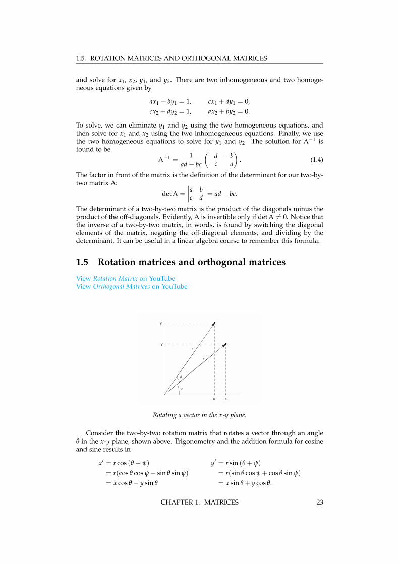
Rotating a vector in the x-y plane.
Consider the two-by-two rotation matrix that rotates a vector through an angleθ in the x-y plane, shown above. Trigonometry and the addition formula for cosineand sine results in
x′ = r cos (θ + ψ) y′ = r sin (θ + ψ)
= r(cos θ cos ψ− sin θ sin ψ) = r(sin θ cos ψ + cos θ sin ψ)
= x cos θ − y sin θ = x sin θ + y cos θ.
CHAPTER 1. MATRICES 23

1.6. MATRIX REPRESENTATION OF COMPLEX NUMBERS
Writing the equations for x′ and y′ in matrix form, we have(x′
y′
)=
(cos θ − sin θsin θ cos θ
)(xy
).
The above two-by-two matrix is called a rotation matrix and is given by
Rθ =
(cos θ − sin θsin θ cos θ
).
Example: Find the inverse of the rotation matrix Rθ .The inverse of Rθ rotates a vector clockwise by θ. To find R−1
θ , we need only changeθ → −θ:
R−1θ = R−θ =
(cos θ sin θ− sin θ cos θ
).
This result agrees with (1.4) since det Rθ = 1.Notice that R−1
θ = RTθ . In general, a square n-by-n matrix Q with real entries
that satisfiesQ−1 = QT
is called an orthogonal matrix. Since QQT = I and QTQ = I, and since QQT multipliesthe rows of Q against themselves, and QTQ multiplies the columns of Q againstthemselves, both the rows of Q and the columns of Q must form an orthonormalset of vectors (normalized and mutually orthogonal). For example, the columnvectors of R, given by (
cos θsin θ
),(− sin θ
cos θ
),
are orthonormal.It is clear that rotating a vector around the origin doesn’t change its length.
More generally, orthogonal matrices preserve inner products. To prove, let Q be anorthogonal matrix and x a column vector. Then
(Qx)T(Qx) = xTQTQx = xTx.
The complex matrix analogue of an orthogonal matrix is a unitary matrix U.Here, the relationship is
U−1 = U†.
Like Hermitian matrices, unitary matrices also play a fundamental role in quantumphysics.
1.6 Matrix representation of complex numbers
In our studies of complex numbers, we noted that multiplication of a complexnumber by eiθ rotates that complex number an angle θ in the complex plane. Thisleads to the idea that we might be able to represent complex numbers as matriceswith eiθ as the rotation matrix.
Accordingly, we begin by representing eiθ as the rotation matrix, that is,
eiθ =
(cos θ − sin θsin θ cos θ
)= cos θ
(1 00 1
)+ sin θ
(0 −11 0
).
24 CHAPTER 1. MATRICES
1.7. PERMUTATION MATRICES
Since eiθ = cos θ + i sin θ, we are led to the matrix representations of the unit num-bers as
1 =
(1 00 1
), i =
(0 −11 0
).
A general complex number z = x + iy is then represented as
z =
(x −yy x
).
The complex conjugate operation, where i → −i, is seen to be just the matrixtranspose.Example: Show that i2 = −1 in the matrix representation.We have
i2 =
(0 −11 0
)(0 −11 0
)=
(−1 0
0 −1
)= −
(1 00 1
)= −1.
Example: Show that zz = x2 + y2 in the matrix representation.We have
zz =
(x −yy x
)(x y−y x
)=
(x2 + y2 0
0 x2 + y2
)= (x2 + y2)
(1 00 1
)= (x2 + y2).
We can now see that there is a one-to-one correspondence between the set of com-plex numbers and the set of all two-by-two matrices with equal diagonal elementsand opposite off-diagonal elements. If you do not like the idea of
√−1, then just
imagine the arithmetic of these two-by-two matrices!
1.7 Permutation matrices
View Permutation Matrices on YouTube
A permutation matrix is another type of orthogonal matrix. When multiplied onthe left, an n-by-n permutation matrix reorders the rows of an n-by-n matrix, andwhen multiplied on the right, reorders the columns. For example, let the string 12represent the order of the rows (columns) of a two-by-two matrix. Then the permu-tations of the rows (columns) are given by 12 and 21. The first permutation is nopermutation at all, and the corresponding permutation matrix is simply the identitymatrix. The second permutation of the rows (columns) is achieved by(
0 11 0
)(a bc d
)=
(c da b
),(
a bc d
)(0 11 0
)=
(b ad c
).
The rows (columns) of a 3-by-3 matrix has 3! = 6 possible permutations, namely123, 132, 213, 231, 312, 321. For example, the row permutation 312 is obtained by0 0 1
1 0 00 1 0
a b cd e fg h i
=
g h ia b cd e f
.
Evidently, the permutation matrix is obtained by permutating the correspondingrows of the identity matrix. Because the columns and rows of the identity matrixare orthonormal, the permutation matrix is an orthogonal matrix.
CHAPTER 1. MATRICES 25
1.8. PROJECTION MATRICES
1.8 Projection matrices
The two-by-two projection matrix projects a vector onto a specified vector in the x-yplane. Let u be a unit vector in R2. The projection of an arbitrary vector x = 〈x1, x2〉onto the vector u = 〈u1, u2〉 is determined from
Proju(x) = (x · u)u = (x1u1 + x2u2)〈u1, u2〉.
In matrix form, this becomes(p1p2
)=
(u2
1 u1u2u1u2 u2
2
)(x1x2
).
The projection matrix Pu, then, can be defined as
Pu =
(u2
1 u1u2u1u2 u2
2
)=
(u1u2
) (u1 u2
)= uuT,
which is an outer product. Notice that Pu is symmetric.Example: Show that P2
u = Pu.It should be obvious that two projections is the same as one. To prove, we have
P2u = (uuT)(uuT)
= u(uTu)uT (associative law)
= uuT (u is a unit vector)= Pu.
26 CHAPTER 1. MATRICES
Chapter 2
Systems of linear equationsConsider the system of n linear equations and n unknowns, given by
a11x1 + a12x2 + · · ·+ a1nxn = b1,a21x1 + a22x2 + · · ·+ a2nxn = b2,
......
an1x1 + an2x2 + · · ·+ annxn = bn.
We can write this system as the matrix equation
Ax = b, (2.1)
with
A =
a11 a12 · · · a1na21 a22 · · · a2n...
.... . .
...an1 an2 · · · ann
, x =
x1x2...
xn
, b =
b1b2...
bn
.
This chapter details the standard algorithm to solve (2.1).
2.1 Gaussian Elimination
View Gaussian Elimination on YouTube
The standard algorithm to solve a system of linear equations is called Gaussianelimination. It is easiest to illustrate this algorithm by example.
Consider the linear system of equations given by
−3x1 + 2x2 − x3 = −1,6x1 − 6x2 + 7x3 = −7,3x1 − 4x2 + 4x3 = −6,
(2.2)
which can be rewritten in matrix form as−3 2 −16 −6 73 −4 4
x1x2x3
=
−1−7−6
.
To perform Gaussian elimination, we form what is called an augmented matrix bycombining the matrix A with the column vector b:−3 2 −1 −1
6 −6 7 −73 −4 4 −6
.
Row reduction is then performed on this matrix. Allowed operations are (1) mul-tiply any row by a constant, (2) add a multiple of one row to another row, (3)
27
2.2. WHEN THERE IS NO UNIQUE SOLUTION
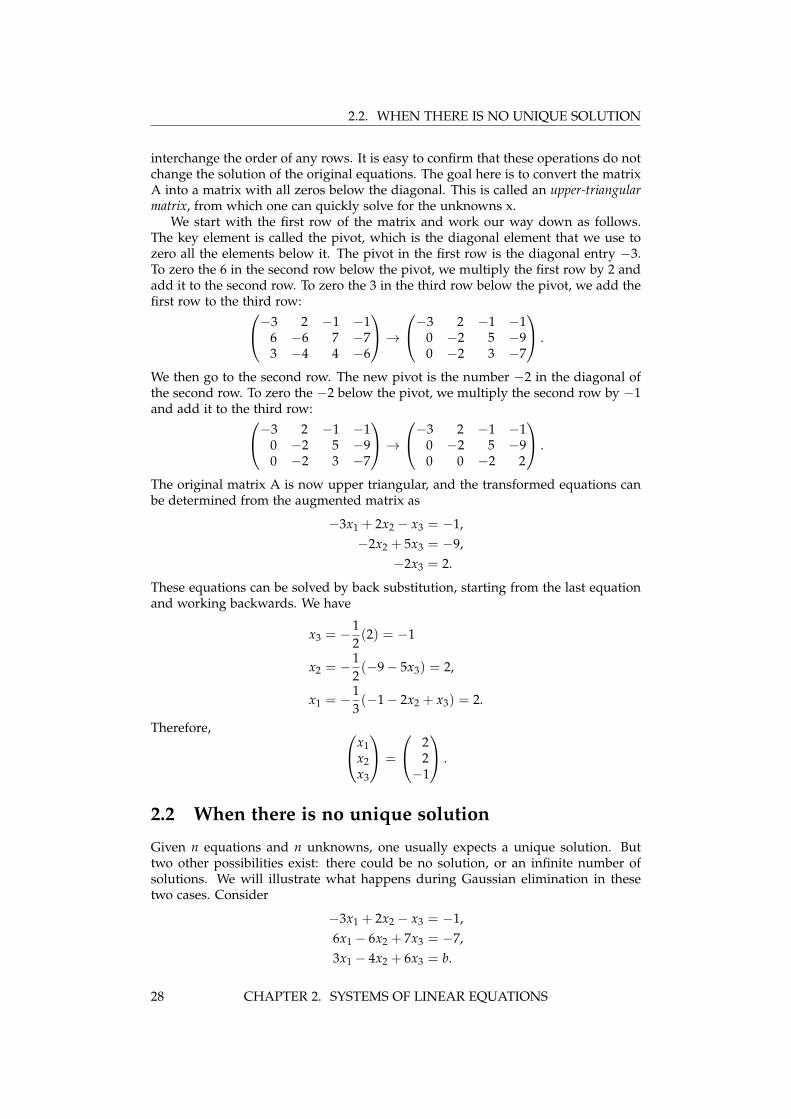
interchange the order of any rows. It is easy to confirm that these operations do notchange the solution of the original equations. The goal here is to convert the matrixA into a matrix with all zeros below the diagonal. This is called an upper-triangularmatrix, from which one can quickly solve for the unknowns x.
We start with the first row of the matrix and work our way down as follows.The key element is called the pivot, which is the diagonal element that we use tozero all the elements below it. The pivot in the first row is the diagonal entry −3.To zero the 6 in the second row below the pivot, we multiply the first row by 2 andadd it to the second row. To zero the 3 in the third row below the pivot, we add thefirst row to the third row:−3 2 −1 −1
6 −6 7 −73 −4 4 −6
→−3 2 −1 −1
0 −2 5 −90 −2 3 −7
.
We then go to the second row. The new pivot is the number −2 in the diagonal ofthe second row. To zero the −2 below the pivot, we multiply the second row by −1and add it to the third row:−3 2 −1 −1
0 −2 5 −90 −2 3 −7
→−3 2 −1 −1
0 −2 5 −90 0 −2 2
.
The original matrix A is now upper triangular, and the transformed equations canbe determined from the augmented matrix as
−3x1 + 2x2 − x3 = −1,−2x2 + 5x3 = −9,
−2x3 = 2.
These equations can be solved by back substitution, starting from the last equationand working backwards. We have
x3 = −12(2) = −1
x2 = −12(−9− 5x3) = 2,
x1 = −13(−1− 2x2 + x3) = 2.
Therefore, x1x2x3
=
22−1
.
2.2 When there is no unique solution
Given n equations and n unknowns, one usually expects a unique solution. Buttwo other possibilities exist: there could be no solution, or an infinite number ofsolutions. We will illustrate what happens during Gaussian elimination in thesetwo cases. Consider
−3x1 + 2x2 − x3 = −1,6x1 − 6x2 + 7x3 = −7,3x1 − 4x2 + 6x3 = b.
28 CHAPTER 2. SYSTEMS OF LINEAR EQUATIONS
2.3. REDUCED ROW ECHELON FORM
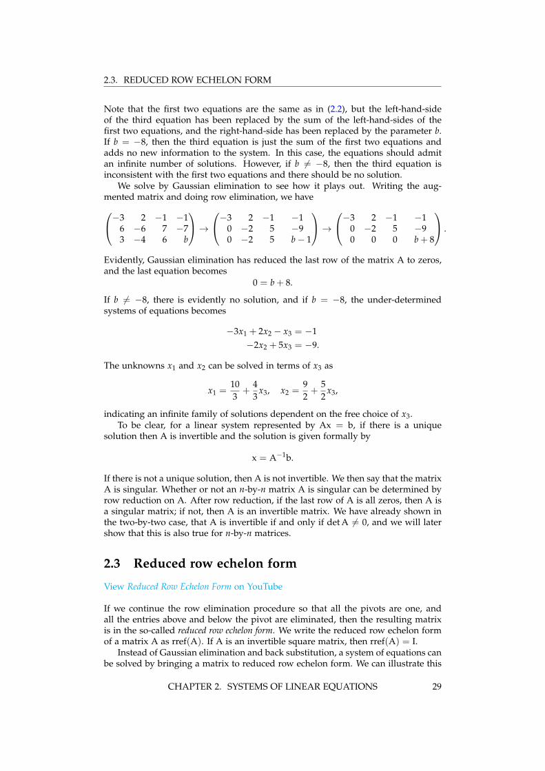
Note that the first two equations are the same as in (2.2), but the left-hand-sideof the third equation has been replaced by the sum of the left-hand-sides of thefirst two equations, and the right-hand-side has been replaced by the parameter b.If b = −8, then the third equation is just the sum of the first two equations andadds no new information to the system. In this case, the equations should admitan infinite number of solutions. However, if b 6= −8, then the third equation isinconsistent with the first two equations and there should be no solution.
We solve by Gaussian elimination to see how it plays out. Writing the aug-mented matrix and doing row elimination, we have−3 2 −1 −1
6 −6 7 −73 −4 6 b
→−3 2 −1 −1
0 −2 5 −90 −2 5 b− 1
→−3 2 −1 −1
0 −2 5 −90 0 0 b + 8
.
Evidently, Gaussian elimination has reduced the last row of the matrix A to zeros,and the last equation becomes
0 = b + 8.
If b 6= −8, there is evidently no solution, and if b = −8, the under-determinedsystems of equations becomes
−3x1 + 2x2 − x3 = −1−2x2 + 5x3 = −9.
The unknowns x1 and x2 can be solved in terms of x3 as
x1 =103
+43
x3, x2 =92+
52
x3,
indicating an infinite family of solutions dependent on the free choice of x3.To be clear, for a linear system represented by Ax = b, if there is a unique
solution then A is invertible and the solution is given formally by
x = A−1b.
If there is not a unique solution, then A is not invertible. We then say that the matrixA is singular. Whether or not an n-by-n matrix A is singular can be determined byrow reduction on A. After row reduction, if the last row of A is all zeros, then A isa singular matrix; if not, then A is an invertible matrix. We have already shown inthe two-by-two case, that A is invertible if and only if det A 6= 0, and we will latershow that this is also true for n-by-n matrices.
2.3 Reduced row echelon form
View Reduced Row Echelon Form on YouTube
If we continue the row elimination procedure so that all the pivots are one, andall the entries above and below the pivot are eliminated, then the resulting matrixis in the so-called reduced row echelon form. We write the reduced row echelon formof a matrix A as rref(A). If A is an invertible square matrix, then rref(A) = I.
Instead of Gaussian elimination and back substitution, a system of equations canbe solved by bringing a matrix to reduced row echelon form. We can illustrate this
CHAPTER 2. SYSTEMS OF LINEAR EQUATIONS 29
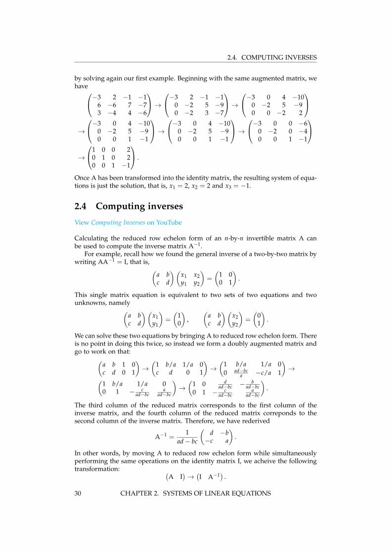
2.4. COMPUTING INVERSES
by solving again our first example. Beginning with the same augmented matrix, wehave−3 2 −1 −1
6 −6 7 −73 −4 4 −6
→−3 2 −1 −1
0 −2 5 −90 −2 3 −7
→−3 0 4 −10
0 −2 5 −90 0 −2 2
→
−3 0 4 −100 −2 5 −90 0 1 −1
→−3 0 4 −10
0 −2 5 −90 0 1 −1
→−3 0 0 −6
0 −2 0 −40 0 1 −1
→
1 0 0 20 1 0 20 0 1 −1
.
Once A has been transformed into the identity matrix, the resulting system of equa-tions is just the solution, that is, x1 = 2, x2 = 2 and x3 = −1.
2.4 Computing inverses
View Computing Inverses on YouTube
Calculating the reduced row echelon form of an n-by-n invertible matrix A canbe used to compute the inverse matrix A−1.
For example, recall how we found the general inverse of a two-by-two matrix bywriting AA−1 = I, that is, (
a bc d
)(x1 x2y1 y2
)=
(1 00 1
).
This single matrix equation is equivalent to two sets of two equations and twounknowns, namely(
a bc d
)(x1y1
)=
(10
),
(a bc d
)(x2y2
)=
(01
).
We can solve these two equations by bringing A to reduced row echelon form. Thereis no point in doing this twice, so instead we form a doubly augmented matrix andgo to work on that:(
a b 1 0c d 0 1
)→(
1 b/a 1/a 0c d 0 1
)→(
1 b/a 1/a 00 ad−bc
a −c/a 1
)→(
1 b/a 1/a 00 1 − c
ad−bca
ad−bc
)→(
1 0 dad−bc − b
ad−bc0 1 − c
ad−bca
ad−bc
).
The third column of the reduced matrix corresponds to the first column of theinverse matrix, and the fourth column of the reduced matrix correponds to thesecond column of the inverse matrix. Therefore, we have rederived
A−1 =1
ad− bc
(d −b−c a
).
In other words, by moving A to reduced row echelon form while simultaneouslyperforming the same operations on the identity matrix I, we acheive the followingtransformation: (
A I)→(I A−1) .
30 CHAPTER 2. SYSTEMS OF LINEAR EQUATIONS
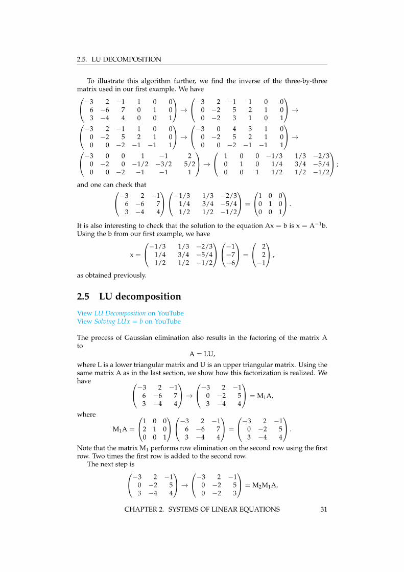
2.5. LU DECOMPOSITION
To illustrate this algorithm further, we find the inverse of the three-by-threematrix used in our first example. We have−3 2 −1 1 0 0
6 −6 7 0 1 03 −4 4 0 0 1
→−3 2 −1 1 0 0
0 −2 5 2 1 00 −2 3 1 0 1
→−3 2 −1 1 0 0
0 −2 5 2 1 00 0 −2 −1 −1 1
→−3 0 4 3 1 0
0 −2 5 2 1 00 0 −2 −1 −1 1
→−3 0 0 1 −1 2
0 −2 0 −1/2 −3/2 5/20 0 −2 −1 −1 1
→ 1 0 0 −1/3 1/3 −2/3
0 1 0 1/4 3/4 −5/40 0 1 1/2 1/2 −1/2
;
and one can check that−3 2 −16 −6 73 −4 4
−1/3 1/3 −2/31/4 3/4 −5/41/2 1/2 −1/2
=
1 0 00 1 00 0 1
.
It is also interesting to check that the solution to the equation Ax = b is x = A−1b.Using the b from our first example, we have
x =
−1/3 1/3 −2/31/4 3/4 −5/41/2 1/2 −1/2
−1−7−6
=
22−1
,
as obtained previously.
2.5 LU decomposition
View LU Decomposition on YouTubeView Solving LUx = b on YouTube
The process of Gaussian elimination also results in the factoring of the matrix Ato
A = LU,
where L is a lower triangular matrix and U is an upper triangular matrix. Using thesame matrix A as in the last section, we show how this factorization is realized. Wehave −3 2 −1
6 −6 73 −4 4
→−3 2 −1
0 −2 53 −4 4
= M1A,
where
M1A =
1 0 02 1 00 0 1
−3 2 −16 −6 73 −4 4
=
−3 2 −10 −2 53 −4 4
.
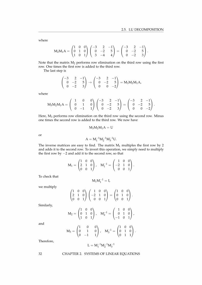
Note that the matrix M1 performs row elimination on the second row using the firstrow. Two times the first row is added to the second row.
The next step is−3 2 −10 −2 53 −4 4
→−3 2 −1
0 −2 50 −2 3
= M2M1A,
CHAPTER 2. SYSTEMS OF LINEAR EQUATIONS 31
2.5. LU DECOMPOSITION
where
M2M1A =
1 0 00 1 01 0 1
−3 2 −10 −2 53 −4 4
=
−3 2 −10 −2 50 −2 3
.
Note that the matrix M2 performs row elimination on the third row using the firstrow. One times the first row is added to the third row.
The last step is−3 2 −10 −2 50 −2 3
→−3 2 −1
0 −2 50 0 −2
= M3M2M1A,
where
M3M2M1A =
1 0 00 1 00 −1 1
−3 2 −10 −2 50 −2 3
=
−3 2 −10 −2 50 0 −2
.
Here, M3 performs row elimination on the third row using the second row. Minusone times the second row is added to the third row. We now have
M3M2M1A = U
orA = M−1
1 M−12 M−1
3 U.
The inverse matrices are easy to find. The matrix M1 multiples the first row by 2and adds it to the second row. To invert this operation, we simply need to multiplythe first row by −2 and add it to the second row, so that
M1 =
1 0 02 1 00 0 1
, M−11 =
1 0 0−2 1 0
0 0 1
.
To check thatM1M−1
1 = I,
we multiply 1 0 02 1 00 0 1
1 0 0−2 1 0
0 0 1
=
1 0 00 1 00 0 1
.
Similarly,
M2 =
1 0 00 1 01 0 1
, M−12 =
1 0 00 1 0−1 0 1
,
and
M3 =
1 0 00 1 00 −1 1
, M−13 =
1 0 00 1 00 1 1
.
Therefore,L = M−1
1 M−12 M−1
3
32 CHAPTER 2. SYSTEMS OF LINEAR EQUATIONS
2.5. LU DECOMPOSITION
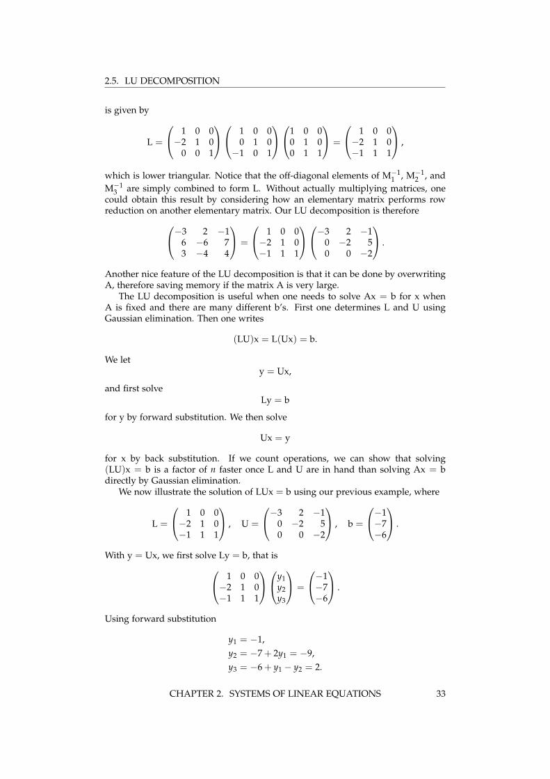
is given by
L =
1 0 0−2 1 0
0 0 1
1 0 00 1 0−1 0 1
1 0 00 1 00 1 1
=
1 0 0−2 1 0−1 1 1
,
which is lower triangular. Notice that the off-diagonal elements of M−11 , M−1
2 , andM−1
3 are simply combined to form L. Without actually multiplying matrices, onecould obtain this result by considering how an elementary matrix performs rowreduction on another elementary matrix. Our LU decomposition is therefore−3 2 −1
6 −6 73 −4 4
=
1 0 0−2 1 0−1 1 1
−3 2 −10 −2 50 0 −2
.
Another nice feature of the LU decomposition is that it can be done by overwritingA, therefore saving memory if the matrix A is very large.
The LU decomposition is useful when one needs to solve Ax = b for x whenA is fixed and there are many different b’s. First one determines L and U usingGaussian elimination. Then one writes
(LU)x = L(Ux) = b.
We lety = Ux,
and first solveLy = b
for y by forward substitution. We then solve
Ux = y
for x by back substitution. If we count operations, we can show that solving(LU)x = b is a factor of n faster once L and U are in hand than solving Ax = bdirectly by Gaussian elimination.
We now illustrate the solution of LUx = b using our previous example, where
L =
1 0 0−2 1 0−1 1 1
, U =
−3 2 −10 −2 50 0 −2
, b =
−1−7−6
.
With y = Ux, we first solve Ly = b, that is 1 0 0−2 1 0−1 1 1
y1y2y3
=
−1−7−6
.
Using forward substitution
y1 = −1,y2 = −7 + 2y1 = −9,y3 = −6 + y1 − y2 = 2.
CHAPTER 2. SYSTEMS OF LINEAR EQUATIONS 33
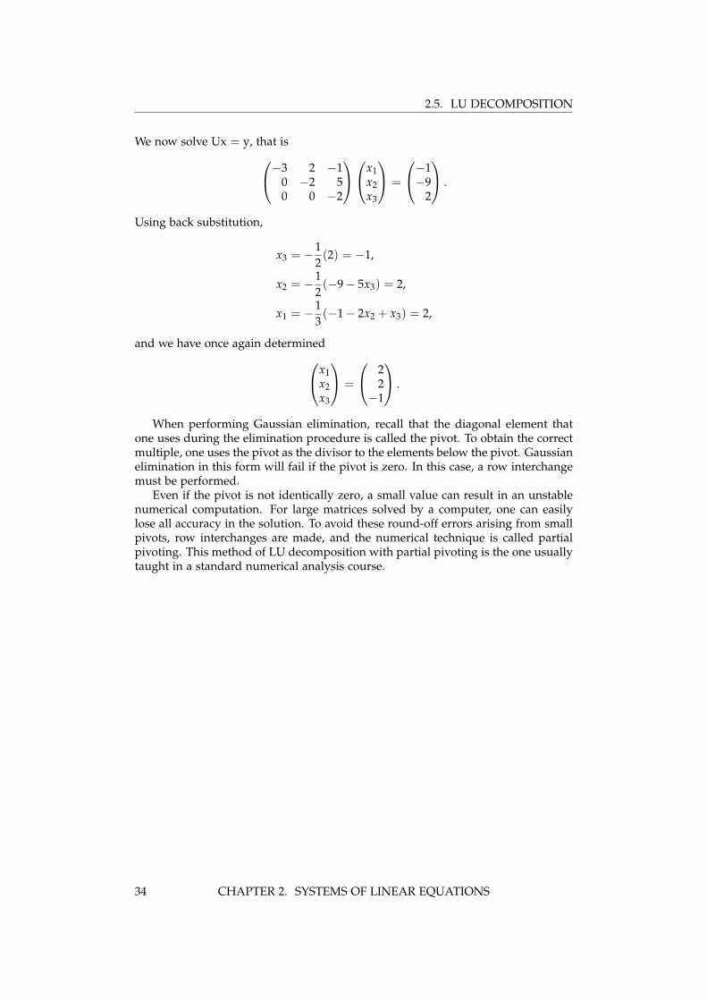
2.5. LU DECOMPOSITION
We now solve Ux = y, that is−3 2 −10 −2 50 0 −2
x1x2x3
=
−1−9
2
.
Using back substitution,
x3 = −12(2) = −1,
x2 = −12(−9− 5x3) = 2,
x1 = −13(−1− 2x2 + x3) = 2,
and we have once again determinedx1x2x3
=
22−1
.
When performing Gaussian elimination, recall that the diagonal element thatone uses during the elimination procedure is called the pivot. To obtain the correctmultiple, one uses the pivot as the divisor to the elements below the pivot. Gaussianelimination in this form will fail if the pivot is zero. In this case, a row interchangemust be performed.
Even if the pivot is not identically zero, a small value can result in an unstablenumerical computation. For large matrices solved by a computer, one can easilylose all accuracy in the solution. To avoid these round-off errors arising from smallpivots, row interchanges are made, and the numerical technique is called partialpivoting. This method of LU decomposition with partial pivoting is the one usuallytaught in a standard numerical analysis course.
34 CHAPTER 2. SYSTEMS OF LINEAR EQUATIONS
Chapter 3
Vector spacesLinear algebra abstracts the vector concept, introducing new vocabulary and defi-nitions that are widely used by scientists and engineers. Vector spaces, subspaces,inner product spaces, linear combinations, linear independence, linear dependence,span, basis, dimension, norm, unit vectors, orthogonal, orthonormal: this is thevocabulary that you need to know.
3.1 Vector spaces
View Vector Spaces on YouTube
In multivariable, or vector calculus, a vector is defined to be a mathematical con-struct that has both direction and magnitude. In linear algebra, vectors are definedmore abstractly. Vectors are mathematical constructs that can be added and multi-plied by scalars under the usual rules of arithmetic. Vector addition is commutativeand associative, and scalar multiplication is distributive and associative. Let u, v,and w be vectors, and let a, b, and c be scalars. Then the rules of arithmetic say that
u + v = v + u, u + (v + w) = (u + v) + w;
anda(u + v) = au + av, a(bu) = (ab)u.
A vector space consists of a set of vectors and a set of scalars that is closed undervector addition and scalar multiplication. That is, when you multiply any twovectors in a vector space by scalars and add them, the resulting vector is still in thevector space.
We can give some examples of vector spaces. Let the scalars be the set of realnumbers and let the vectors be column matrices of a specified type. One exampleof a vector space is the set of all three-by-one column matrices. If we let
u =
u1u2u3
, v =
v1v2v3
,
then
w = au + bv =
au1 + bv1au2 + bv2au3 + bv3
is evidently a three-by-one matrix, so that the set of all three-by-one matrices (to-gether with the set of real numbers) forms a vector space. This vector space isusually called R3.
A vector subspace is a vector space that is a subset of another vector space. Forexample, a vector subspace of R3 could be the set of all three-by-one matrices withzero in the third row. If we let
u =
u1u20
, v =
v1v20
,
35
3.1. VECTOR SPACES
then
w = au + bv =
au1 + bv1au2 + bv2
0
is evidently also a three-by-one matrix with zero in the third row. This subspaceof R3 is closed under scalar multiplication and vector addition and is therefore avector space. Another example of a vector subspace of R3 would be the set of allthree-by-one matrices where the first row is equal to the third row.
Of course, not all subsets of R3 form a vector space. A simple example wouldbe the set of all three-by-one matrices where the row elements sum to one. If, say,u =
(1 0 0
)T, then au is a vector whose rows sum to a, which can be differentthan one.
The zero vector must be a member of every vector space. If u is in the vectorspace, then so is 0u which is just the zero vector. Another argument would be thatif u is in the vector space, then so is (−1)u = −u, and u− u is again equal to thezero vector.
The concept of vector spaces is more general than a set of column matrices. Hereare some examples where the vectors are functions.Example: Consider vectors consisting of all real polynomials in x of degree lessthan or equal to n. Show that this set of vectors (together with the set of realnumbers) form a vector space.Consider the polynomials of degree less than or equal to n given by
p(x) = a0 + a1x + a2x2 + · · ·+ anxn, q(x) = b0 + b1x + b2x2 + · · ·+ bnxn,
where a0, a1, . . . , an and b0, b1, . . . , bn are real numbers. Clearly, multiplying thesepolynmials by real numbers still results in a polynomial of degree less than or equalto n. Adding these polynomials results in
p(x) + q(x) = (a0 + b0) + (a1 + b1)x + (a2 + b2)x2 + · · ·+ (an + bn)xn,
which is another polynomial of degree less than or equal to n. Since this set ofpolynomials is closed under scalar multiplication and vector addition, it forms avector space. This vector space is designated as Pn.Example: Consider a function y = y(x) and the differential equation d3y/dx3 = 0.Find the vector space associated with the general solution of this differentialequation.From Calculus, we know that the function whose third derivative is zero is a poly-nomial of degree less than or equal to two. That is, the general solution to thedifferential equation is
y(x) = a0 + a1x + a2x2,which is just all possible vectors in the vector space P2.Example: Consider a function y = y(x) and the differential equation d2y/dx2 +y = 0. Find the vector space associated with the general solution of this differen-tial equation.Again from Calculus, we know that the trigonometric functions cos x and sin x havesecond derivatives that are the negative of themselves. The general solution to thedifferential equation consists of all vectors of the form
y(x) = a cos x + b sin x,
which is just all possible vectors in the vector space consisting of a linear combina-tion of cos x and sin x.
36 CHAPTER 3. VECTOR SPACES
3.2. LINEAR INDEPENDENCE
3.2 Linear independence
View Linear Independence on YouTube
A set of vectors, {u1, u2, . . . , un}, are said to be linearly independent if for anyscalars c1, c2, . . . , cn, the equation
c1u1 + c2u2 + · · ·+ cnun = 0
has only the solution c1 = c2 = · · · = cn = 0. What this means is that one is unableto write any of the vectors u1, u2, . . . , un as a linear combination of any of the othervectors. For instance, if there was a solution to the above equation with c1 6= 0,then we could solve that equation for u1 in terms of the other vectors with nonzerocoefficients.
As an example consider whether the following three three-by-one column vec-tors are linearly independent:
u =
100
, v =
010
, w =
230
.
Indeed, they are not linearly independent, that is, they are linearly dependent, be-cause w can be written in terms of u and v. In fact, w = 2u + 3v. Now consider thethree three-by-one column vectors given by
u =
100
, v =
010
, w =
001
.
These three vectors are linearly independent because you cannot write any one ofthese vectors as a linear combination of the other two. If we go back to our definitionof linear independence, we can see that the equation
au + bv + cw =
abb
=
000
has as its only solution a = b = c = 0.
3.3 Span, basis and dimension
View Span, Basis and Dimension on YouTube
Given a set of vectors, one can generate a vector space by forming all linear com-binations of that set of vectors. The span of the set of vectors {v1, v2, . . . , vn} is thevector space consisting of all linear combinations of v1, v2, . . . , vn. We say that a setof vectors spans a vector space.
For example, the set of three-by-one column matrices given by1
00
,
010
,
230
CHAPTER 3. VECTOR SPACES 37
3.3. SPAN, BASIS AND DIMENSION
spans the vector space of all three-by-one matrices with zero in the third row. Thisvector space is a vector subspace of all three-by-one matrices.
One doesn’t need all three of these vectors to span this vector subspace becauseany one of these vectors is linearly dependent on the other two. The smallest setof vectors needed to span a vector space forms a basis for that vector space. Here,given the set of vectors above, we can construct a basis for the vector subspace ofall three-by-one matrices with zero in the third row by simply choosing two out ofthree vectors from the above spanning set. Three possible bases are given by
100
,
010
,
1
00
,
230
,
0
10
,
230
.
Although all three combinations form a basis for the vector subspace, the first com-bination is usually preferred because this is an orthonormal basis. The vectors inthis basis are mutually orthogonal and of unit norm.
The number of vectors in a basis gives the dimension of the vector space. Here,the dimension of the vector space of all three-by-one matrices with zero in the thirdrow is two.Example: Find an orthonormal basis for the set of all three-by-one matrices wherethe first row is equal to the third row.There are many different solutions to this example, but a rather simple orthonormalbasis is given by
010
,
√22
101
.
Any other three-by-one matrix with first row equal to third row can be written asa linear combination of these two basis vectors, and the dimension of this vectorspace is also two.
Example: Determine a basis for P2, the vector space consisting of all polynomialsof degree less than or equal to two. Again, there are many possible choices for abasis, but perhaps the simplest one is given by{
1, x, x2}
.
Clearly, any polynomial of degree less than or equal to two can be written as alinear combination of these basis vectors. The dimension of P2 is three.
Example: Determine a basis for the vector space given by the general solutionof the differential equation d2y/dx2 + y = 0. The general solution is given by
y(x) = a cos x + b sin x,
and a basis for this vector space are just the functions
{cos x, sin x} .
The dimension of the vector space given by the general solution of the differentialequation is two. This dimension is equal to the order of the highest derivative inthe differential equation.
38 CHAPTER 3. VECTOR SPACES
3.4. INNER PRODUCT SPACES
3.4 Inner product spaces
We have discussed the inner product (or dot product) between two column matrices.Recall that the inner product between, say, two three-by-one column matrices
u =
u1u2u3
, v =
v1v2v3
is given by
uTv = u1v1 + u2v2 + u3v3.
We now generalize the inner product so that it is applicable to any vector space,including those containing functions.
We will denote the inner product between any two vectors u and v as (u, v), andrequire the inner product to satisfy the same arithmetic rules that are satisfied bythe dot product. With u, v, w vectors and c a scalar, these rules can be written as
(u, v) = (v, u), (u + v, w) = (u, w) + (v, w), (cu, v) = c(u, v) = (u, cv);
and (u, u) ≥ 0, where the equality holds if and only if u = 0.Generalizing our definitions for column matrices, the norm of a vector u is de-
fined as||u|| = (u, u)1/2.
A unit vector is a vector whose norm is one. Unit vectors are said to be normalized tounity, though sometimes we just say that they are normalized. We say two vectors areorthogonal if their inner product is zero. We also say that a basis is orthonormal (as inan orthonormal basis) if all the vectors are mutually orthogonal and are normalizedto unity. For an orthonormal basis consisting of the vectors v1, v2, . . . , vn, we write
(vi, vj) = δij,
where δij is called the Kronecker delta, defined as
δij =
{1, if i = j;0, if i 6= j.
Oftentimes, basis vectors are used that are orthogonal but are normalized to othervalues besides unity.Example: Define an inner product for Pn.Let p(x) and q(x) be two polynomials in Pn. One possible definition of an innerproduct is given by
(p, q) =∫ 1
−1p(x)q(x)dx.
You can check that all the conditions of an inner product are satisfied.Example: Show that the first four Legendre polynomials form an orthogonal basisfor P3 using the inner product defined above.The first four Legendre polynomials are given by
P0(x) = 1, P1(x) = x, P2(x) =12(3x2 − 1), P3(x) =
12(5x3 − 3x),
CHAPTER 3. VECTOR SPACES 39
3.5. VECTOR SPACES OF A MATRIX
and these four polynomials form a basis for P3. With an inner product defined onPn as
(p, q) =∫ 1
−1p(x)q(x)dx,
it can be shown by explicit integration that
(Pm, Pn) =2
2n + 1δm,n,
so that the first four Legendre polynomials are mutually orthogonal. They arenormalized so that Pn(1) = 1.
Example: Define an inner product on Pn such that the Hermite polynomials areorthogonal.
For instance, the first four Hermite polynomials are given by
H0(x) = 1, H1(x) = 2x, H2(x) = 4x2 − 2, H3(x) = 8x3 − 12x,
which also form a basis for P3. Here, define an inner product on Pn as
(p, q) =∫ ∞
−∞p(x)q(x)e−x2
dx.
It can be shown that
(Hm, Hn) = 2nπ1/2n!δm,n,
so that the Hermite polynomials are orthogonal with this definition of the innerproduct. These Hermite polynomials are normalized so that the leading coefficientof Hn is given by 2n.
3.5 Vector spaces of a matrix
3.5.1 Null space
View Null Space on YouTube
The null space of a matrix A is the vector space spanned by all vectors x that satisfythe matrix equation
Ax = 0.
If the matrix A is m-by-n, then the column vector x is n-by-one and the null space ofA is a subspace of Rn. If A is a square invertible matrix, then the null space consistsof just the zero vector.
To find a basis for the null space of a noninvertible matrix, we bring A to rowreduced echelon form. We demonstrate by example. Consider the three-by-fivematrix given by
A =
−3 6 −1 1 −71 −2 2 3 −12 −4 5 8 −4
.
40 CHAPTER 3. VECTOR SPACES

3.5. VECTOR SPACES OF A MATRIX
By judiciously permuting rows to simplify the arithmetic, one pathway to constructrref(A) is−3 6 −1 1 −7
1 −2 2 3 −12 −4 5 8 −4
→ 1 −2 2 3 −1−3 6 −1 1 −7
2 −4 5 8 −4
→1 −2 2 3 −1
0 0 5 10 −100 0 1 2 −2
→1 −2 2 3 −1
0 0 1 2 −20 0 5 10 −10
→1 −2 0 −1 3
0 0 1 2 −20 0 0 0 0
.
We can now write the matrix equation Ax = 0 for the null space using rref(A).Writing the variable associated with the pivot columns on the left-hand-side of theequations, we have from the first and second rows
x1 = 2x2 + x4 − 3x5,x3 = −2x4 + 2x5.
Eliminating x1 and x3, we now write the general solution for vectors in the nullspace as
2x2 + x4 − 3x5x2
−2x4 + 2x5x4x5
= x2
21000
+ x4
10−2
10
+ x5
−3
0201
,
where x2, x4, and x5 are called free variables, and can take any values. By writingthe null space in this form, a basis for the null space is made evident, and is givenby
21000
,
10−2
10
,
−3
0201
.
The null space is seen to be a three-dimensional subspace of R5, and its dimensionis equal to the number of free variables of rref(A). The number of free variables is,of course, equal to the number of columns minus the number of pivot columns.
3.5.2 Application of the null space
View Application of the Null Space on YouTube
An underdetermined system of linear equations Ax = b with more unknownsthan equations may not have a unique solution. If u is the general form of a vectorin the null space of A, and v is any vector that satisfies Av = b, then x = u + vsatisfies Ax = A(u + v) = Au + Av = 0 + b = b. The general solution of Ax = bcan therefore be written as the sum of a general vector in Null(A) and a particularvector that satisfies the underdetermined system.
CHAPTER 3. VECTOR SPACES 41
3.5. VECTOR SPACES OF A MATRIX
As an example, suppose we want to find the general solution to the linear systemof two equations and three unknowns given by
2x1 + 2x2 + x3 = 0,2x1 − 2x2 − x3 = 1,
which in matrix form is given by
(2 2 12 −2 −1
)x1x2x3
=
(01
).
We first bring the augmented matrix to reduced row echelon form:(2 2 1 02 −2 −1 1
)→(
1 0 0 1/40 1 1/2 −1/4
).
The null space is determined from x1 = 0 and x2 = −x3/2, and we can write
Null(A) = span
0−1
2
.
A particular solution for the inhomogeneous system is found by solving x1 = 1/4and x2 + x3/2 = −1/4. Here, we simply take the free variable x3 to be zero, and wefind x1 = 1/4 and x2 = −1/4. The general solution to the original underdeterminedlinear system is the sum of the null space and the particular solution and is givenby x1
x2x3
= a
0−1
2
+14
1−1
0
.
3.5.3 Column spaceView Column Space on YouTube
The column space of a matrix is the vector space spanned by the columns of thematrix. When a matrix is multiplied by a column vector, the resulting vector is inthe column space of the matrix, as can be seen from the example(
a bc d
)(xy
)=
(ax + bycx + dy
)= x
(ac
)+ y
(bd
).
In general, Ax is a linear combination of the columns of A, and the equation Ax = 0expresses the linear dependence of the columns of A.
Given an m-by-n matrix A, what is the dimension of the column space of A, andhow do we find a basis? Note that since A has m rows, the column space of A is asubspace of Rm.
Fortunately, a basis for the column space of A can be found from rref(A). Con-sider the example of §3.5.1, where
A =
−3 6 −1 1 −71 −2 2 3 −12 −4 5 8 −4
,
42 CHAPTER 3. VECTOR SPACES
3.5. VECTOR SPACES OF A MATRIX
and
rref(A) =
1 −2 0 −1 30 0 1 2 −20 0 0 0 0
.
The matrix equation Ax = 0 is equivalent to rref(A)x = 0, and the latter equationcan be expressed as
x1
100
+ x2
−200
+ x3
010
+ x4
−120
+ x5
3−2
0
=
000
.
Only the pivot columns of rref(A), here the first and third columns, are linearlyindependent. For example, the second column is −2 times the first column; andwhatever linear dependence relations hold for rref(A) hold true for the originalmatrix A. (You can try and check this fact.) The dimension of the column space ofA is therefore equal to the number of pivot columns of A, and here it is two. A basisfor the column space is given by the first and third columns of A (not rref(A)), andis
−312
,
−125
.
Recall that the dimension of the null space is the number of non-pivot columns,so that the sum of the dimensions of the null space and the column space is equalto the total number of columns. A statement of this theorem is as follows. Let A bean m-by-n matrix. Then
dim(Col(A)) + dim(Null(A)) = n.
3.5.4 Row space, left null space and rankView Row Space, Left Null Space and Rank on YouTube
In addition to the column space and the null space, a matrix A has two more vectorspaces associated with it, namely the column space and null space of AT, which arecalled the row space and the left null space of A.
If A is an m-by-n matrix, then the row space and the null space are subspaces ofRn, and the column space and the left null space are subspaces of Rm.
The null space consists of all vectors x such that Ax = 0, that is, the null spaceis the set of all vectors that are orthogonal to the row space of A. We say that thesetwo vector spaces are orthogonal.
A basis for the row space of a matrix can be found from computing rref(A),and is found to be rows of rref(A) (written as column vectors) with pivot columns.The dimension of the row space of A is therefore equal to the number of pivotcolumns, while the dimension of the null space of A is equal to the number ofnonpivot columns. The union of these two subspaces make up the vector space ofall n-by-one matrices and we say that these subspaces are orthogonal complements ofeach other.
Furthermore, the dimension of the column space of A is also equal to the numberof pivot columns, so that the dimensions of the column space and the row space ofa matrix are equal. We have
dim(Col(A)) = dim(Row(A)).
CHAPTER 3. VECTOR SPACES 43
3.6. GRAM-SCHMIDT PROCESS
We call this dimension the rank of the matrix A. This is an amazing result sincethe column space and row space are subspaces of two different vector spaces. Ingeneral, we must have rank(A) ≤ min(m, n). When the equality holds, we say thatthe matrix is of full rank. And when A is a square matrix and of full rank, then thedimension of the null space is zero and A is invertible.
We summarize our results in the table below. The null space of AT is also calledthe left null space of A and the column space of AT is also called the row space ofA. The null space of A and the row space of A are orthogonal complements as isthe left null space of A and the column space of A. The dimension of the columnspace of A is equal to the dimension of the row space of A and this dimension iscalled the rank of A.
Table 3.1: The four fundamental subspaces of an m-by-n matrix
vector space subspace of dimension
Null(A) Rn n− # of pivot columnsCol(A) Rm # of pivot columnsNull(AT) Rm m− # of pivot columnsCol(AT) Rn # of pivot columns
3.6 Gram-Schmidt process
View Gram-Schmidt Process on YouTubeView Gram-Schmidt Process Example on YouTube
Given any basis for a vector space, we can use an algorithm called the Gram-Schmidt process to construct an orthonormal basis for that space. Let the vectorsv1, v2, . . . , vn be a basis for some n-dimensional vector space. We will assume herethat these vectors are column matrices, but this process also applies more generally.
We will construct an orthogonal basis u1, u2, . . . , un, and then normalize eachvector to obtain an orthonormal basis. First, define u1 = v1. To find the next or-thogonal basis vector, define
u2 = v2 −(uT
1 v2)u1
uT1 u1
.
Observe that u2 is equal to v2 minus the component of v2 that is parallel to u1. Bymultiplying both sides of this equation with uT
1 , it is easy to see that uT1 u2 = 0 so
that these two vectors are orthogonal.The next orthogonal vector in the new basis can be found from
u3 = v3 −(uT
1 v3)u1
uT1 u1
−(uT
2 v3)u2
uT2 u2
.
Here, u3 is equal to v3 minus the components of v3 that are parallel to u1 and u2. Wecan continue in this fashion to construct n orthogonal basis vectors. These vectorscan then be normalized via
u1 =u1
(uT1 u1)1/2
, etc.
44 CHAPTER 3. VECTOR SPACES
3.7. ORTHOGONAL PROJECTIONS
Since uk is a linear combination of v1, v2, . . . , vk, the vector subspace spannedby the first k basis vectors of the original vector space is the same as the subspacespanned by the first k orthonormal vectors generated through the Gram-Schmidtprocess. We can write this result as
span{u1, u2, . . . , uk} = span{v1, v2, . . . , vk}.
To give an example of the Gram-Schmidt process, consider a subspace of R4
with the following basis:
W =
1111
,
0111
,
0011
= {v1, v2, v3} .
We use the Gram-Schmidt process to construct an orthonormal basis for this sub-space. Let u1 = v1. Then u2 is found from
u2 = v2 −(uT
1 v2)u1
uT1 u1
=
0111
− 34
1111
=14
−3
111
.
Finally, we compute u3:
u3 = v3 −(uT
1 v3)u1
uT1 u1
−(uT
2 v3)u2
uT2 u2
=
0011
− 12
1111
− 16
−3
111
=13
0−2
11
.
Normalizing the three vectors, we obtain the orthonormal basis
W ′ =
12
1111
,1
2√
3
−3
111
,1√6
0−2
11
.
3.7 Orthogonal projections
View Orthogonal Projections on YouTube
Suppose that V is an n-dimensional vector space and W is a p-dimensional sub-space of V. Let {s1, s2, . . . , sp} be an orthonormal basis for W. Extending the basisfor W, let {s1, s2, . . . , sp, t1, t2, . . . , tn−p} be an orthonormal basis for V.
Any vector v in V can be written in terms of the basis for V as
v = a1s1 + a2s2 + · · ·+ apsp + b1t1 + b2t2 + bn−ptn−p.
CHAPTER 3. VECTOR SPACES 45
3.8. QR FACTORIZATION
The orthogonal projection of v onto W is then defined as
vprojW = a1s1 + a2s2 + · · ·+ apsp,
that is, the part of v that lies in W.If you only know the vector v and the orthonormal basis for W, then the orthog-
onal projection of v onto W can be computed from
vprojW = (vTs1)s1 + (vTs2)s2 + · · ·+ (vTsp)sp,
that is, a1 = vTs1, a2 = vTs2, etc.We can prove that the vector vprojW is the vector in W that is closest to v. Let w
be any vector in W different than vprojW , and expand w in terms of the basis vectorsfor W:
w = c1s1 + c2s2 + · · ·+ cpsp.
The distance between v and w is given by the norm ||v−w||, and we have
||v−w||2 = (a1 − c1)2 + (a2 − c2)
2 + · · ·+ (ap − cp)2 + b2
1 + b22 + · · ·+ b2
n−p
≥ b21 + b2
2 + · · ·+ b2n−p = ||v− vprojW ||
2,
or ||v− vprojW || ≤ ||v−w||, a result that will be used later in the problem of leastsquares.
3.8 QR factorization
The Gram-Schmidt process naturally leads to a matrix factorization. Let A be an m-by-n matrix with n linearly-independent columns given by {x1, x2, . . . , xn}. Follow-ing the Gram-Schmidt process, it is always possible to construct an orthornormalbasis for the column space of A, denoted by {q1, q2, . . . , qn}. An important featureof this orthonormal basis is that the first k basis vectors from the orthonormal setspan the same vector subspace as the first k columns of the matrix A. For somecoefficients rij, we can therefore write
x1 = r11q1,x2 = r12q1 + r22q2,x3 = r13q1 + r23q2 + r33q3,
......
xn = r1nq1 + r2nq2 + · · ·+ rnnqn;
and these equations can be written in matrix form asx1 x2 x3 . . . xn
=
q1 q2 q3 . . . qn
r11 r12 . . . r1n0 r22 . . . r2n...
......
...0 0 . . . rnn
.
This form represents the matrix factorization called the QR factorization, and isusually written as
A = QR,
46 CHAPTER 3. VECTOR SPACES
3.9. THE LEAST-SQUARES PROBLEM
where Q is an orthogonal matrix and R is an upper triangular matrix. The diagonalelements of R can also be made non-negative by suitably adjusting the signs of theorthonormal basis vectors.
As a concrete example, we will find the the QR factorization of the matrix
A =
(1 22 1
)=
a1 a2
.
Applying the Gram-Schmidt process to the column vectors of A, we have for theunnormalized orthogonal vectors
q1 = a1 =
(12
),
q2 = a2 −(qT
1 a2)q1
qT1 q1
=
(21
)− 4
5
(12
)=
(6/5−3/5
)=
35
(2−1
),
and normalizing, we obtain
q1 =1√5
(12
), q2 =
1√5
(2−1
).
The projection of the columns of A onto the set of orthonormal vectors is given by
a1 = (aT1 q1)q1, a2 = (aT
2 q1)q1 + (aT2 q2)q2,
and with rij = aTj qi, we compute
r11 = aT1 q1 =
(1 2
) (12
)1√5=√
5,
r12 = aT2 q1 =
(2 1
) (12
)1√5=
4√
55
,
r22 = aT2 q2 =
(2 1
) ( 2−1
)1√5=
3√
55
.
The QR factorization of A is therefore given by(1 22 1
)=
(1/√
5 2/√
52/√
5 −1/√
5
)(√5 4√
5/50 3
√5/5
).
3.9 The least-squares problem
View The Least-Squares Problem Using Matrices on YouTube
Suppose there is some experimental data that is suspected to satisfy a functionalrelationship. The simplest such relationship is linear, and suppose one wants to fita straight line to the data. An example of such a linear regression problem is shownin Fig. 3.1.
CHAPTER 3. VECTOR SPACES 47
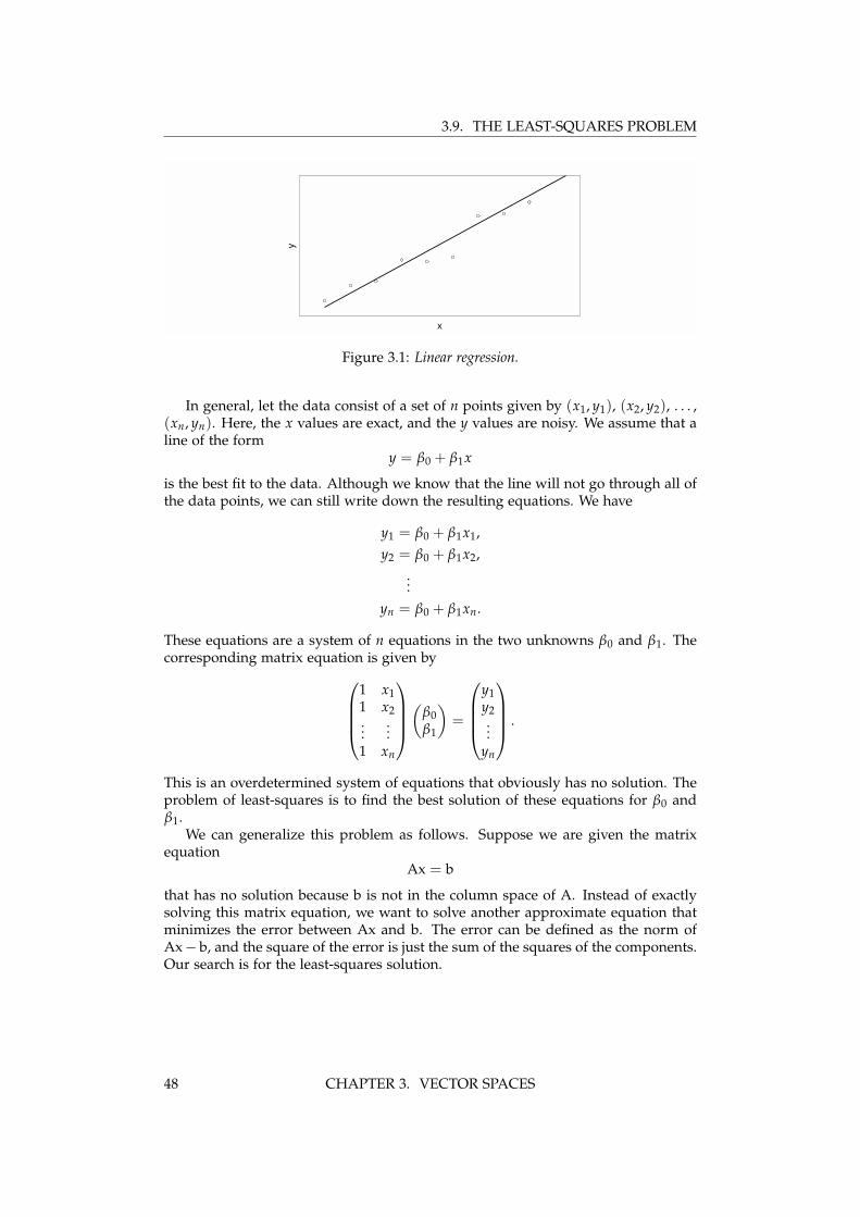
3.9. THE LEAST-SQUARES PROBLEM
x
y
Figure 3.1: Linear regression.
In general, let the data consist of a set of n points given by (x1, y1), (x2, y2), . . . ,(xn, yn). Here, the x values are exact, and the y values are noisy. We assume that aline of the form
y = β0 + β1x
is the best fit to the data. Although we know that the line will not go through all ofthe data points, we can still write down the resulting equations. We have
y1 = β0 + β1x1,y2 = β0 + β1x2,
...yn = β0 + β1xn.
These equations are a system of n equations in the two unknowns β0 and β1. Thecorresponding matrix equation is given by
1 x11 x2...
...1 xn
(
β0β1
)=
y1y2...
yn
.
This is an overdetermined system of equations that obviously has no solution. Theproblem of least-squares is to find the best solution of these equations for β0 andβ1.
We can generalize this problem as follows. Suppose we are given the matrixequation
Ax = b
that has no solution because b is not in the column space of A. Instead of exactlysolving this matrix equation, we want to solve another approximate equation thatminimizes the error between Ax and b. The error can be defined as the norm ofAx− b, and the square of the error is just the sum of the squares of the components.Our search is for the least-squares solution.
48 CHAPTER 3. VECTOR SPACES

3.10. SOLUTION OF THE LEAST-SQUARES PROBLEM
3.10 Solution of the least-squares problem
View Solution of the Least-Squares Problem by the Normal Equations on YouTube
The problem of least-squares can be cast as the problem of solving an overdeter-mined matrix equation Ax = b when b is not in the column space of A. By replacingb by its orthogonal projection onto the column space of A, the solution minimizesthe norm ||Ax− b||.
Now b = bprojCol(A)+ (b− bprojCol(A)
), where bprojCol(A)is the projection of b onto
the column space of A. Since (b− bprojCol(A)) is orthogonal to the column space of
A, it is in the nullspace of AT. Therefore, AT(b− bprojCol(A)) = 0, and it pays to
multiply Ax = b by AT to obtain
ATAx = ATb.
These equations, called the normal equations for Ax = b, determine the least-squares solution for x, which can be found by Gaussian elimination. When A isan m-by-n matrix, then ATA is an n-by-n matrix, and it can be shown that ATA isinvertible when the columns of A are linearly independent. When this is the case,one can rewrite the normal equations by multiplying both sides by A(ATA)−1 toobtain
Ax = A(ATA)−1ATb,
where the matrixP = A(ATA)−1AT
projects a vector onto the column space of A. It is easy to prove that P2 = P, whichstates that two projections is the same as one. We have
P2 = (A(ATA)−1AT)(A(ATA)−1AT)
= A[(ATA)−1(ATA)
](ATA)−1AT
= A(ATA)−1AT = P.
As an example, consider the toy least-squares problem of fitting a line throughthe three data points (1, 1), (2, 3) and (3, 2). With the line given by y = β0 + β1x,the overdetermined system of equations is given by1 1
1 21 3
(β0β1
)=
132
.
The least-squares solution is determined by solving
(1 1 11 2 3
)1 11 21 3
(β0β1
)=
(1 1 11 2 3
)132
,
or (3 66 14
)(β0β1
)=
(613
).
CHAPTER 3. VECTOR SPACES 49
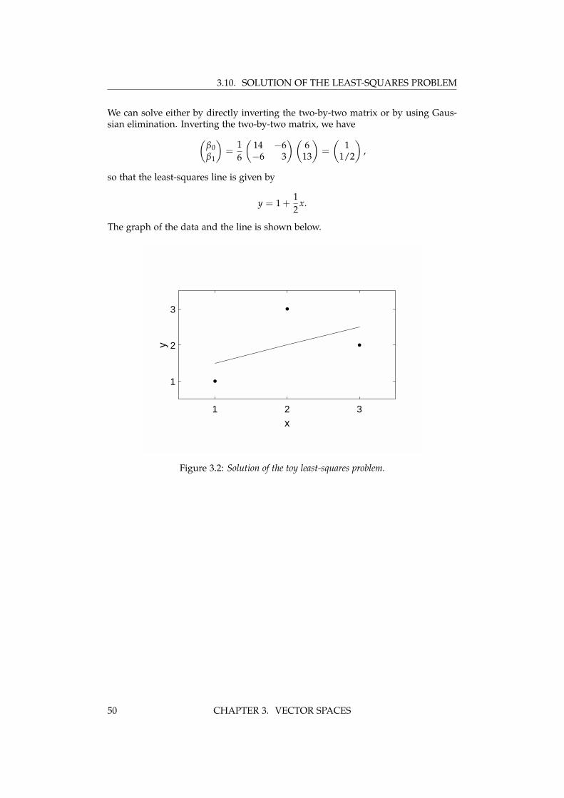
3.10. SOLUTION OF THE LEAST-SQUARES PROBLEM
We can solve either by directly inverting the two-by-two matrix or by using Gaus-sian elimination. Inverting the two-by-two matrix, we have(
β0β1
)=
16
(14 −6−6 3
)(6
13
)=
(1
1/2
),
so that the least-squares line is given by
y = 1 +12
x.
The graph of the data and the line is shown below.
1 2 3
x
1
2
3
y
Figure 3.2: Solution of the toy least-squares problem.
50 CHAPTER 3. VECTOR SPACES
Chapter 4
Determinants4.1 Two-by-two and three-by-three determinants
View Two-by-Two and Three-by-Three Determinants on YouTube
Our first introduction to determinants was the definition for the general two-by-two matrix
A =
(a bc d
): det A = ad− bc.
Other widely used notations for the determinant include
det A = det(
a bc d
)= |A| =
∣∣∣∣a bc d
∣∣∣∣ .
By explicit construction, we have seen that a two-by-two matrix A is invertible ifand only if det A 6= 0. If a square matrix A is invertible, then the equation Ax = bhas the unique solution x = A−1b. But if A is not invertible, then Ax = b may haveno solution or an infinite number of solutions. When det A = 0, we say that A is asingular matrix.
Here, we would like to extend the definition of the determinant to an n-by-nmatrix. Before we do so, let us display the determinant for a three-by-three matrix.We consider the system of equations Ax = 0 and find the condition for which x = 0is the only solution. This condition must be equivalent to det A 6= 0. Witha b c
d e fg h i
x1x2x3
= 0,
one can do the messy algebra of elimination to solve for x1, x2, and x3. One findsthat x1 = x2 = x3 = 0 is the only solution when det A 6= 0, where the definition isgiven by
det A = aei + b f g + cdh− ceg− bdi− a f h. (4.1)
A way to remember this result for the three-by-three matrix is by the followingpicture:
a b c a b
d e f d e
g h i g h
-
a b c a b
d e f d e
g h i g h
.
The matrix A is periodically extended two columns to the right, drawn explicitlyhere but usually only imagined. Then the six terms comprising the determinant aremade evident, with the lines slanting down towards the right getting the plus signsand the lines slanting down towards the left getting the minus signs. Unfortunately,this mnemonic is only valid for three-by-three matrices.
51
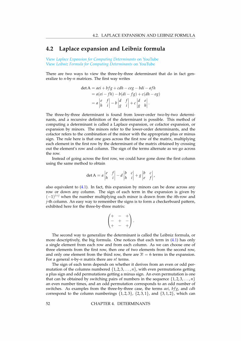
4.2. LAPLACE EXPANSION AND LEIBNIZ FORMULA
4.2 Laplace expansion and Leibniz formula
View Laplace Expansion for Computing Determinants on YouTubeView Leibniz Formula for Computing Determinants on YouTube
There are two ways to view the three-by-three determinant that do in fact gen-eralize to n-by-n matrices. The first way writes
det A = aei + b f g + cdh− ceg− bdi− a f h= a(ei− f h)− b(di− f g) + c(dh− eg)
= a∣∣∣∣e fh i
∣∣∣∣− b∣∣∣∣d fg i
∣∣∣∣+ c∣∣∣∣d eg h
∣∣∣∣ .
The three-by-three determinant is found from lower-order two-by-two determi-nants, and a recursive definition of the determinant is possible. This method ofcomputing a determinant is called a Laplace expansion, or cofactor expansion, orexpansion by minors. The minors refer to the lower-order determinants, and thecofactor refers to the combination of the minor with the appropriate plus or minussign. The rule here is that one goes across the first row of the matrix, multiplyingeach element in the first row by the determinant of the matrix obtained by crossingout the element’s row and column. The sign of the terms alternate as we go acrossthe row.
Instead of going across the first row, we could have gone done the first columnusing the same method to obtain
det A = a∣∣∣∣e fh i
∣∣∣∣− d∣∣∣∣b ch i
∣∣∣∣+ g∣∣∣∣b ce f
∣∣∣∣ ,
also equivalent to (4.1). In fact, this expansion by minors can be done across anyrow or down any column. The sign of each term in the expansion is given by(−1)i+j when the number multiplying each minor is drawn from the ith-row andj-th column. An easy way to remember the signs is to form a checkerboard pattern,exhibited here for the three-by-three matrix:+ − +
− + −+ − +
.
The second way to generalize the determinant is called the Leibniz formula, ormore descriptively, the big formula. One notices that each term in (4.1) has onlya single element from each row and from each column. As we can choose one ofthree elements from the first row, then one of two elements from the second row,and only one element from the third row, there are 3! = 6 terms in the expansion.For a general n-by-n matrix there are n! terms.
The sign of each term depends on whether it derives from an even or odd per-mutation of the columns numbered {1, 2, 3, . . . , n}, with even permutations gettinga plus sign and odd permutations getting a minus sign. An even permutation is onethat can be obtained by switching pairs of numbers in the sequence {1, 2, 3, . . . , n}an even number times, and an odd permutation corresponds to an odd number ofswitches. As examples from the three-by-three case, the terms aei, b f g, and cdhcorrespond to the column numberings {1, 2, 3}, {2, 3, 1}, and {3, 1, 2}, which can
52 CHAPTER 4. DETERMINANTS
4.3. PROPERTIES OF THE DETERMINANT
be seen to be even permutations of {1, 2, 3}, and the terms ceg, bdi, and a f h cor-respond to the column numberings {3, 2, 1}, {2, 1, 3}, and {1, 3, 2}, which are oddpermutations.
Either the Laplace expansion or the Leibniz formula can be used to define thedeterminant of an n-by-n matrix.
It will, however, be more fun to define the determinant from three more funda-mental properties. These properties will lead us to the most important conditiondet A 6= 0 for an invertible matrix. But we will also elucidate many other usefulproperties.
4.3 Properties of the determinant
View Properties of the Determinant on YouTube
The determinant, as we know, is a function that maps an n-by-n matrix to a scalar.We now define this determinant function by the following three properties.
Property 1: The determinant of the identity matrix is one, i.e.,
det I = 1.
This property essentially normalizes the determinant. The two-by-two illustrationis ∣∣∣∣1 0
0 1
∣∣∣∣ = 1× 1− 0× 0 = 1.
Property 2: The determinant changes sign under row exchange. The two-by-twoillustration is ∣∣∣∣a b
c d
∣∣∣∣ = ad− bc = −(cb− da) = −∣∣∣∣c da b
∣∣∣∣ .
Property 3: The determinant is a linear function of the first row, holding all otherrows fixed. The two-by-two illustration is∣∣∣∣ka kb
c d
∣∣∣∣ = kad− kbc = k(ad− bc) = k∣∣∣∣a bc d
∣∣∣∣and∣∣∣∣a + a′ b + b′
c d
∣∣∣∣ = (a + a′)d− (b + b′)c = (ad− bc) + (a′d− b′c) =∣∣∣∣a bc d
∣∣∣∣+ ∣∣∣∣a′ b′
c d
∣∣∣∣ .
Remarkably, Properties 1-3 are all we need to uniquely define the determinant func-tion. It can be shown that these three properties hold in both the two-by-two andthree-by-three cases, and for the Laplace expansion and the Leibniz formula for thegeneral n-by-n case.
We now discuss further properties that follow from Properties 1-3. We willcontinue to illustrate these properties using a two-by-two matrix.
CHAPTER 4. DETERMINANTS 53

4.3. PROPERTIES OF THE DETERMINANT
Property 4: The determinant is a linear function of all the rows, e.g.,∣∣∣∣ a bkc kd
∣∣∣∣ = − ∣∣∣∣kc kda b
∣∣∣∣ (Property 2)
= −k∣∣∣∣c da b
∣∣∣∣ (Property 3)
= k∣∣∣∣a bc d
∣∣∣∣ , (Property 2)
and similarly for the second linearity condition.
Property 5: If a matrix has two equal rows, then the determinant is zero, e.g.,∣∣∣∣a ba b
∣∣∣∣ = − ∣∣∣∣a ba b
∣∣∣∣ (Property 2)
= 0,
since zero is the only number equal to its negative.
Property 6: If we add k times row-i to row-j the determinant doesn’t change, e.g.,∣∣∣∣ a bc + ka d + kb
∣∣∣∣ = ∣∣∣∣a bc d
∣∣∣∣+ k∣∣∣∣a ba b
∣∣∣∣ (Property 4)
=
∣∣∣∣a bc d
∣∣∣∣ . (Property 5)
This property together with Property 2 and 3 allows us to perform Gaussian elimi-nation on a matrix to simplify the calculation of a determinant.
Property 7: The determinant of a matrix with a row of zeros is zero, e.g.,∣∣∣∣a b0 0
∣∣∣∣ = 0∣∣∣∣a b0 0
∣∣∣∣ (Property 4)
= 0.
Property 8: The determinant of a diagonal matrix is just the product of the diagonalelements, e.g., ∣∣∣∣a 0
0 d
∣∣∣∣ = ad∣∣∣∣1 00 1
∣∣∣∣ (Property 4)
= ad. (Property 1)
Property 9: The determinant of an upper or lower triangular matrix is just the prod-uct of the diagonal elements, e.g., ∣∣∣∣a b
0 d
∣∣∣∣ = ∣∣∣∣a 00 d
∣∣∣∣ (Property 6)
= ad. (Property 8)
In the above calculation, Property 6 is applied by multiplying the second row by−b/d and adding it to the first row.
54 CHAPTER 4. DETERMINANTS
4.3. PROPERTIES OF THE DETERMINANT
Property 10: A matrix with a nonzero determinant is invertible. A matrix with azero determinant is singular. Row reduction (Property 6), row exchange (Property2), and multiplication of a row by a nonzero scalar (Property 4) can bring a squarematrix to its reduced row echelon form. If rref(A) = I, then the determinant isnonzero and the matrix is invertible. If rref(A) 6= I, then the last row is all zeros,the determinant is zero, and the matrix is singular.
Property 11: The determinant of the product is equal to the product of the determi-nants, i.e.,
det AB = det A det B.
This identity turns out to be very useful, but its proof for a general n-by-n matrix isdifficult. The proof for a two-by-two matrix can be done directly. Let
A =
(a bc d
), B =
(e fg h
).
Then
AB =
(ae + bg a f + bhce + dg c f + dh
),
and
det AB =
∣∣∣∣ae + bg a f + bhce + dg c f + dh
∣∣∣∣=
∣∣∣∣ ae a fce + dg c f + dh
∣∣∣∣+ ∣∣∣∣ bg bhce + dg c f + dh
∣∣∣∣=
∣∣∣∣ae a fce c f
∣∣∣∣+ ∣∣∣∣ae a fdg dh
∣∣∣∣+ ∣∣∣∣bg bhce c f
∣∣∣∣+ ∣∣∣∣bg bhdg dh
∣∣∣∣= ac
∣∣∣∣e fe f
∣∣∣∣+ ad∣∣∣∣e fg h
∣∣∣∣+ bc∣∣∣∣g he f
∣∣∣∣+ bd∣∣∣∣g hg h
∣∣∣∣= (ad− bc)
∣∣∣∣e fg h
∣∣∣∣= det A det B.
Property 12: Commuting two matrices doesn’t change the value of the determinant,i.e., det AB = det BA. The proof is simply
det AB = det A det B (Property 11)= det B det A= det BA. (Property 11)
Property 13: The determinant of the inverse is the inverse of the determinant, i.e., ifA is invertible, then det (A−1) = 1/ det A. The proof is
1 = det I (Property 1)
= det (AA−1)
= det A det A−1. (Property 11)
CHAPTER 4. DETERMINANTS 55
4.3. PROPERTIES OF THE DETERMINANT
Therefore,
det A−1 =1
det A.
Property 14: The determinant of a matrix raised to an integer power is equal tothe determinant of that matrix, raised to the integer power. Note that A2 = AA,A3 = AAA, etc. This property in equation form is given by
det (Ap) = (det A)p,
where p is an integer. This result follows from the successive application of Property11.
Property 15: If A is an n-by-n matrix, then
det kA = kn det A.
Note that kA multiplies every element of A by the scalar k. This property followssimply from Property 4 applied n times.
Property 16: The determinant of the transposed matrix is equal to the determinantof the matrix, i.e.
det AT = det A.
When A = LU without any row exchanges, we have AT = UTLT and
det AT = det UTLT
= det UT det LT (Property 11)= det U det L (Property 9)= det LU (Property 11)= det A.
The same result can be shown to hold even if row interchanges are needed. Theimplication of Property 16 is that any statement about the determinant and the rowsof A also apply to the columns of A. To compute the determinant, one can do eitherrow reduction or column reduction!
It is time for some examples. We start with a simple three-by-three matrix andillustrate some approaches to a hand calculation of the determinant.Example: Compute the determinant of
A =
1 5 02 4 −10 −2 0
.
We show computations using the Leibniz formula and the Laplace expansion.Method 1 (Leibniz formula): We compute the six terms directly by periodically extend-ing the matrix and remembering that diagonals slanting down towards the right getplus signs and diagonals slanting down towards the left get minus signs. We have
det A = 1 · 4 · 0 + 5 · (−1) · 0 + 0 · 2 · (−2)− 0 · 4 · 0− 5 · 2 · 0− 1 · (−1) · (−2) = −2.
Method 2 (Laplace expansion): We expand using minors. We should choose an expan-sion across the row or down the column that has the most zeros. Here, the obvious
56 CHAPTER 4. DETERMINANTS
4.3. PROPERTIES OF THE DETERMINANT
choices are either the third row or the third column, and we can show both. Acrossthe third row, we have
det A = −(−2) ·∣∣∣∣1 02 −1
∣∣∣∣ = −2,
and down the third column, we have
det A = −(−1) ·∣∣∣∣1 50 −2
∣∣∣∣ = −2.
Example: Compute the determinant of
A =
6 3 2 4 09 0 −4 1 08 −5 6 7 13 0 0 0 04 2 3 2 0
.
We first expand in minors across the fourth row:∣∣∣∣∣∣∣∣∣∣6 3 2 4 09 0 −4 1 08 −5 6 7 13 0 0 0 04 2 3 2 0
∣∣∣∣∣∣∣∣∣∣= −3
∣∣∣∣∣∣∣∣3 2 4 00 −4 1 0−5 6 7 1
2 3 2 0
∣∣∣∣∣∣∣∣ .
We then expand in minors down the fourth column:
−3
∣∣∣∣∣∣∣∣3 2 4 00 −4 1 0−5 6 7 1
2 3 2 0
∣∣∣∣∣∣∣∣ = 3
∣∣∣∣∣∣3 2 40 −4 12 3 2
∣∣∣∣∣∣ .
We can then multiply the third column by 4 and add it to the second column:
= 3
∣∣∣∣∣∣3 2 40 −4 12 3 2
∣∣∣∣∣∣ = 3
∣∣∣∣∣∣3 18 40 0 12 11 2
∣∣∣∣∣∣ ,
and finally expand in minors across the second row:
3
∣∣∣∣∣∣3 18 40 0 12 11 2
∣∣∣∣∣∣ = −3∣∣∣∣3 182 11
∣∣∣∣ = −3(33− 36) = 9.
The technique here is to try and zero out all the elements in a row or a columnexcept one before proceeding to expand by minors across that row or column.Example: Recall the Fibonacci Q-matrix, which satisfies
Q =
(1 11 0
), Qn =
(Fn+1 Fn
Fn Fn−1
),
where Fn is the nth Fibonacci number. Prove Cassini’s identity
Fn+1Fn−1 − F2n = (−1)n.
CHAPTER 4. DETERMINANTS 57
4.4. USE OF DETERMINANTS IN VECTOR CALCULUS
Repeated us of Property 10 yields det (Qn) = (det Q)n. Applying this identity to theFibonacci Q-matrix results in Cassini’s identity. For example, with F5 = 5, F6 = 8,F7 = 13, we have 13 · 5− 82 = 1. Cassini’s identity leads to an amusing dissectionfallacy called the Fibonacci bamboozlement, which I will show you in class.Example: A Hessenberg matrix is an almost upper- or lower-triangular matrix.Consider the lower Hessenberg matrix with twos on the diagonal, ones belowthe diagonal, and ones on the superdiagonal. The matrix denoted by Hn is then-by-n version of this matrix. For example, the first four matrices are given by
H1 =(2)
, H2 =
(2 11 2
), H3 =
2 1 01 2 11 1 2
H4 =
2 1 0 01 2 1 01 1 2 11 1 1 2
.
Show that |Hn| = Fn+2.
Let’s compute the first three determinants. We have |H1| = 2 = F3 and |H2| = 3 =F4. We compute |H3| going across the first row using minors:
|H3| = 2∣∣∣∣2 11 2
∣∣∣∣− ∣∣∣∣1 11 2
∣∣∣∣ = 6− 1 = 5 = F5.
To prove that |Hn| = Fn+2, we need only prove that |Hn+1| = |Hn|+ |Hn−1|. Weexpand |Hn+1| in minors across the first row. It is easy to see that
|Hn+1| = 2|Hn| −
∣∣∣∣∣∣∣∣∣∣∣
1 1 0 0 . . .1 2 1 0 . . .1 1 2 1 . . .1 1 1 2 . . ....
......
... . . .
∣∣∣∣∣∣∣∣∣∣∣.
The remaining determinant of an n-by-n matrix seems problematic, but we canmake use of the linearity property of determinants to write∣∣∣∣∣∣∣∣∣∣∣
1 1 0 0 . . .1 2 1 0 . . .1 1 2 1 . . .1 1 1 2 . . ....
......
... . . .
∣∣∣∣∣∣∣∣∣∣∣=
∣∣∣∣∣∣∣∣∣∣∣
2 1 0 0 . . .1 2 1 0 . . .1 1 2 1 . . .1 1 1 2 . . ....
......
... . . .
∣∣∣∣∣∣∣∣∣∣∣−
∣∣∣∣∣∣∣∣∣∣∣
1 0 0 0 . . .1 2 1 0 . . .1 1 2 1 . . .1 1 1 2 . . ....
......
... . . .
∣∣∣∣∣∣∣∣∣∣∣= |Hn| − |Hn−1|,
where the second determinant on the right-hand-side was evaluated using a Laplaceexpansion across the first row. Putting the result together gives us the Fibonaccirecursion relation |Hn+1| = |Hn|+ |Hn−1|, so that therefore |Hn| = Fn+2.
4.4 Use of determinants in Vector Calculus
Consider two vectors u = u1i + u2j + u3j and v = v1i + v2j + v3j, written as youwould find them in Calculus rather than as column matrices in Linear Algebra. Thedot product of the two vectors is defined in Calculus as
u · v = u1v1 + u2v2 + u3v3,
58 CHAPTER 4. DETERMINANTS
4.4. USE OF DETERMINANTS IN VECTOR CALCULUS
and the cross product is defined as
u× v =
∣∣∣∣∣∣i j k
u1 u2 u3v1 v2 v3
∣∣∣∣∣∣= i(u2v3 − u3v2)− j(u1v3 − u3v1) + k(u1v2 − u2v1),
where the determinant from Linear Algebra is used as a mnemonic to rememberthe definition. If the angle between the two vectors is given by θ, then trigonometrycan be used to show that
u · v = |u||v| cos θ, |u× v| = |u||v| sin θ.
Now, if u and v lie in the x-y plane, then the area of the parallelogram formed fromthese two vectors, determined from base times height, is given by
A = |u× v|= |u1v2 − u2v1|
=
∣∣∣∣det(
u1 u2v1 v2
)∣∣∣∣ .
This result also generalizes to three dimensions. The volume of a parallelopipedformed by the three vectors u, v, and w is given by
V = |u · (v×w)|
=
∣∣∣∣∣∣det
u1 u2 u3v1 v2 v3w1 w2 w3
∣∣∣∣∣∣ .
An important application of this result is the change-of-variable formula for multi-dimensional integration. Consider the double integral
I =∫ ∫
A. . . dxdy
over some unspecified function of x and y and over some designated area A in thex-y plane. Suppose we make a linear transformation from the x-y coordinate systemto some u-v coordinate system. That is, let
u = ax + by, v = cx + dy,
or in matrix notation, (uv
)=
(a bc d
)(xy
).
Observe that the orthonormal basis vectors i and j transform into the vectors ai +cj and bi + dj so that a rectangle in the x-y coordinate system transforms into aparallelogram in the u-v coordinate system. The area A of the parallelogram in theu-v coordinate system is given by
A =
∣∣∣∣det(
a cb d
)∣∣∣∣ = ∣∣∣∣det(
a bc d
)∣∣∣∣ .
CHAPTER 4. DETERMINANTS 59
4.4. USE OF DETERMINANTS IN VECTOR CALCULUS
Notice that because this was a linear transformation, we could have also written thearea as
A =
∣∣∣∣∣∣∣∣det
∂u∂x
∂u∂y
∂v∂x
∂v∂y
∣∣∣∣∣∣∣∣ ,
which is called the Jacobian determinant, or just the Jacobian. This result alsoapplies to infinitesimal areas where a linear approximation can be made, and with
u = u(x, y), v = v(x, y),
the change of variables formula becomes
dudv =
∣∣∣∣det∂(u, v)∂(x, y)
∣∣∣∣ dxdy,
where in general, the Jacobian matrix is defined as
∂(u, v)∂(x, y)
=
∂u∂x
∂u∂y
∂v∂x
∂v∂y
.
Note that sometimes we define the change of coordinates as
x = x(u, v), y = y(u, v),
and the change of variables formula will be
dxdy =
∣∣∣∣det∂(x, y)∂(u, v)
∣∣∣∣ dudv.
We can give two very important examples. The first in two dimensions is thechange of variables from rectangular to polar coordinates. We have
x = r cos θ, y = r sin θ,
and the Jacobian of the transformation is∣∣∣∣det∂(x, y)∂(r, θ)
∣∣∣∣ = ∣∣∣∣cos θ −r sin θsin θ r cos θ
∣∣∣∣ = r.
So to find the area of a circle of radius R, with formula x2 + y2 = R2, we have
∫ R
−R
∫ √R2−y2
−√
R2−y2dx dy =
∫ 2π
0
∫ R
0r dr dθ = πR2.
The second example in three dimensions is from cartesian to spherical coordi-nates. Here,
x = r sin θ cos φ, y = r sin θ sin φ, z = r cos θ.
The Jacobian is∣∣∣∣det∂(x, y, z)∂(r, θ, φ)
∣∣∣∣ =∣∣∣∣∣∣sin θ cos φ r cos θ cos φ −r sin θ sin φsin θ sin φ r cos θ sin φ r sin θ cos φ
cos θ −r sin θ 0
∣∣∣∣∣∣ = r2 sin θ.
60 CHAPTER 4. DETERMINANTS

4.4. USE OF DETERMINANTS IN VECTOR CALCULUS
So to find the area of a sphere of radius R, with formula x2 + y2 + z2 = R2, we have
∫ R
−R
∫ √R2−z2
−√
R2−z2
∫ √R2−y2−z2
−√
R2−y2−z2dx dy dz =
∫ 2π
0
∫ π
0
∫ R
0r2 sin θ dr dθ dφ =
43
πR3.
CHAPTER 4. DETERMINANTS 61

4.4. USE OF DETERMINANTS IN VECTOR CALCULUS
62 CHAPTER 4. DETERMINANTS
Chapter 5
Eigenvalues and eigenvectors5.1 The eigenvalue problem
View The Eigenvalue Problem on YouTubeView Finding Eigenvalues and Eigenvectors (Part 1) on YouTubeView Finding Eigenvalues and Eigenvectors (Part 2) on YouTube
Let A be an n-by-n matrix, x an n-by-1 column vector, and λ a scalar. The eigenvalueproblem for a given matrix A solves
Ax = λx (5.1)
for n eigenvalues λi with corresponding eigenvectors xi. Since Ix = x, where I isthe n-by-n identity matrix, we can rewrite the eigenvalue equation (5.1) as
(A− λI)x = 0. (5.2)
The trivial solution to this equation is x = 0, and for nontrivial solutions to exist, then-by-n matrix A− λI, which is the matrix A with λ subtracted from its diagonal,must be singular. Hence, to determine the nontrivial solutions, we must requirethat
det (A− λI) = 0. (5.3)
Using the big formula for the determinant, one can see that (5.3) is an n-th orderpolynomial equation in λ, and is called the characteristic equation of A. The char-acteristic equation can be solved for the eigenvalues, and for each eigenvalue, acorresponding eigenvector can be determined directly from (5.2).
We can demonstrate how to find the eigenvalues of a general 2-by-2 matrix givenby
A =
(a bc d
).
We have
0 = det (A− λI)
=
∣∣∣∣ a− λ bc d− λ
∣∣∣∣= (a− λ)(d− λ)− bc
= λ2 − (a + d)λ + (ad− bc),
which can be more generally written as
λ2 − Tr A λ + det A = 0, (5.4)
where Tr A is the trace, or sum of the diagonal elements, of the matrix A.Since the characteristic equation of a two-by-two matrix is a quadratic equation,
it can have either (i) two distinct real roots; (ii) two distinct complex conjugate roots;
63

5.1. THE EIGENVALUE PROBLEM
or (iii) one degenerate real root. That is, eigenvalues and eigenvectors can be realor complex, and that for certain defective matrices, there may be less than n distincteigenvalues and eigenvectors.
If λ1 is an eigenvalue of our 2-by-2 matrix A, then the corresponding eigenvectorx1 may be found by solving(
a− λ1 bc d− λ1
)(x11x21
)= 0, (5.5)
where the equation of the second row will always be a multiple of the equation ofthe first row because the determinant of the matrix on the left-hand-side is zero. Theeigenvector x1 can be multiplied by any nonzero constant and still be an eigenvector.We could normalize x1, for instance, by taking x11 = 1 or |x1| = 1, or whatever,depending on our needs.
The equation from the first row of (5.5) is
(a− λ1)x11 + bx21 = 0,
and we could take x11 = 1 to find x21 = (λ1 − a)/b. These results are usuallyderived as needed when given specific matrices.Example: Find the eigenvalues and eigenvectors of the following matrices:(
0 11 0
)and
(3 11 3
).
For
A =
(0 11 0
),
the characteristic equation isλ2 − 1 = 0,
with solutions λ1 = 1 and λ2 = −1. The first eigenvector is found by solving(A− λ1I)x1 = 0, or (
−1 11 −1
)(x11x21
)= 0,
so that x21 = x11. The second eigenvector is found by solving (A− λ2I)x2 = 0, or(1 11 1
)(x12x22
)= 0,
so that x22 = −x12. The eigenvalues and eigenvectors are therefore given by
λ1 = 1, x1 =
(11
); λ2 = −1, x2 =
(1−1
).
To find the eigenvalues and eigenvectors of the second matrix we can follow thissame procedure. Or better yet, we can take a shortcut. Let
A =
(0 11 0
)and B =
(3 11 3
).
We know the eigenvalues and eigenvectors of A and that B = A + 3I. Therefore,with λB representing the eigenvalues of B, and λA representing the eigenvalues ofA, we have
0 = det (B− λBI) = det (A + 3I− λBI) = det (A− (λB − 3)I) = det (A− λAI).
64 CHAPTER 5. EIGENVALUES AND EIGENVECTORS
5.1. THE EIGENVALUE PROBLEM
Therefore, λB = λA + 3 and the eigenvalues of B are 4 and 2. The eigenvectorsremain the same.
It is useful to notice that λ1 + λ2 = Tr A and that λ1λ2 = det A. The analogousresult for n-by-n matrices is also true and worthwhile to remember. In particular,summing the eigenvalues and comparing to the trace of the matrix provides a rapidcheck on your algebra.Example: Find the eigenvalues and eigenvectors of the following matrices(
0 −11 0
)and
(0 10 0
).
For
A =
(0 −11 0
),
the characteristic equation isλ2 + 1 = 0,
with solutions i and −i. Notice that if the matrix A is real, then the complexconjugate of the eigenvalue equation Ax = λx is Ax = λx. So if λ and x is aneigenvalue and eigenvector of a real matrix A then so is the complex conjugates λand x. Eigenvalues and eigenvectors of a real matrix appear as complex conjugatepairs.
The eigenvector associated with λ = i is determined from (A− iI)x = 0, or(−i 1
1 −i
)(x1x2
)= 0,
or x2 = ix1. The eigenvectors and eigenvectors of A are therefore given by
λ = i, X =
(1i
); λ = −i, X =
(1−i
).
For
B =
(0 10 0
),
the characteristic equation isλ2 = 0,
so that there is a degenerate eigenvalue of zero. The eigenvector associated with thezero eigenvalue if found from Bx = 0 and has zero second component. Therefore,this matrix is defective and has only one eigenvalue and eigenvector given by
λ = 0, x =
(10
).
Example: Find the eigenvalues and eigenvectors of the rotation matrix
R =
(cos θ − sin θsin θ cos θ
).
The characteristic equation is given by
λ2 − 2 cos θλ + 1 = 0,
CHAPTER 5. EIGENVALUES AND EIGENVECTORS 65
5.2. MATRIX DIAGONALIZATION
with solution
λ± = cos θ ±√
cos2 θ − 1 = cos θ ± i sin θ = e±iθ .
The eigenvector corresponding to λ = eiθ is found from
−i sin θx1 − sin θx2 = 0,
or x2 = −ix1. Therefore, the eigenvalues and eigenvectors are
λ = eiθ , x =
(1−i
)and their complex conjugates.
5.2 Matrix diagonalization
View Matrix Diagonalization on YouTubeView Powers of a Matrix on YouTubeView Powers of a Matrix Example on YouTube
For concreteness, consider a 2-by-2 matrix A with eigenvalues and eigenvectorsgiven by
λ1, x1 =
(x11x21
); λ2, x2 =
(x12x22
).
Now, consider the matrix product and factorization
A(
x11 x12x21 x22
)=
(λ1x11 λ2x12λ1x21 λ2x22
)=
(x11 x12x21 x22
)(λ1 00 λ2
).
We define S to be the matrix whose columns are the eigenvectors of A, and Λ tobe the diagonal eigenvalue matrix. Then generalizing to any square matrix with acomplete set of eigenvectors, we have
AS = SΛ.
Multiplying both sides on the right or the left by S−1, we have found
A = SΛS−1 or Λ = S−1AS.
To memorize the order of the S matrices in these formulas, just remember that Ashould be multiplied on the right by S.
Diagonalizing a matrix facilitates finding powers of that matrix. For instance,
A2 = (SΛS−1)(SΛS−1) = SΛ2S−1,
where in the 2-by-2 example, Λ2 is simply(λ1 00 λ2
)(λ1 00 λ2
)=
(λ2
1 00 λ2
2
).
In general, Λ2 has the eigenvalues squared down the diagonal. More generally, forp a positive integer,
Ap = SΛpS−1.
66 CHAPTER 5. EIGENVALUES AND EIGENVECTORS

5.2. MATRIX DIAGONALIZATION
Example: Recall the Fibonacci Q-matrix, which satisfies
Q =
(1 11 0
), Qn =
(Fn+1 Fn
Fn Fn−1
).
Using Q and Qn, derive Binet’s formula for Fn.The characteristic equation of Q is given by
λ2 − λ− 1 = 0,
with solutions
λ1 =1 +√
52
= Φ, λ2 =1−√
52
= −φ.
Useful identities are
Φ = 1 + φ, Φ = 1/φ, and Φ + φ =√
5.
The eigenvector corresponding to Φ can be found from
x1 −Φx2 = 0,
and the eigenvector corresponding to −φ can be found from
x1 + φx2 = 0.
Therefore, the eigenvalues and eigenvectors can be written as
λ1 = Φ, x1 =
(Φ1
); λ2 = −φ, x2 =
(−φ
1
).
The eigenvector matrix S becomes
S =
(Φ −φ1 1
);
and the inverse of this 2-by-2 matrix is given by
S−1 =1√5
(1 φ−1 Φ
).
Our diagonalization is therefore
Q =1√5
(Φ −φ1 1
)(Φ 00 −φ
)(1 φ−1 Φ
).
Raising to the nth power, we have
Qn =1√5
(Φ −φ1 1
)(Φn 00 (−φ)n
)(1 φ−1 Φ
)=
1√5
(Φ −φ1 1
)(Φn Φn−1
−(−φ)n −(−φ)n−1
)=
1√5
(Φn+1 − (−φ)n+1 Φn − (−φ)n
Φn − (−φ)n Φn−1 − (−φ)n−1
).
Using Qn written in terms of the Fibonacci numbers, we have derived Binet’s for-mula
Fn =Φn − (−φ)n√
5.
CHAPTER 5. EIGENVALUES AND EIGENVECTORS 67

5.3. SYMMETRIC AND HERMITIAN MATRICES
5.3 Symmetric and Hermitian matrices
When a real matrix A is equal to its transpose, AT = A , we say that the matrix issymmetric. When a complex matrix A is equal to its conjugate transpose, A† = A,we say that the matrix is Hermitian.
One of the reasons symmetric and Hermitian matrices are important is becausetheir eigenvalues are real and their eigenvectors are orthogonal. Let λi and λj beeigenvalues and xi and xj eigenvectors of the possibly complex matrix A. We have
Axi = λixi, Axj = λjxj.
Multiplying the first equation on the left by x†j , and taking the conjugate transpose
of the second equation and multiplying on the right by xi, we obtain
x†j Axi = λix†
j xi, x†j A†xi = λjx†
j xi.
If A is Hermitian, then A† = A, and subtracting the second equation from the firstyields
(λi − λj)x†j xi = 0.
If i = j, then since x†i xi > 0, we have λi = λi: all eigenvalues are real. If i 6= j
and λi 6= λj, then x†j xi = 0: eigenvectors with distinct eigenvalues are orthogonal.
Usually, the eigenvectors are made orthonormal, and diagonalization makes use ofreal orthogonal or complex unitary matrices.Example: Diagonalize the symmetric matrix
A =
(a bb a
).
The characteristic equation of A is given by
(a− λ)2 = b2,
with real eigenvalues λ1 = a+ b and λ2 = a− b. The eigenvector with eigenvalue λ1satisfies −x1 + x2 = 0, and the eigenvector with eigenvalue λ2 satisfies x1 + x2 = 0.Normalizing the eigenvectors, we have
λ1 = a + b, X1 =1√2
(11
); λ2 = a− b, X2 =
1√2
(1−1
).
Evidently, the eigenvectors are orthonormal. The diagonalization using A = QΛQ−1
is given by (a bb a
)=
1√2
(1 11 −1
)(a + b 0
0 a− b
)1√2
(1 11 −1
),
which can be verified directly by matrix multiplication. The matrix Q is a symmetricorthogonal matrix so that Q−1 = Q.
68 CHAPTER 5. EIGENVALUES AND EIGENVECTORS

Part II
Differential equations
69


The second part of this course is on differential equations. We begin with first-order odes and explain how to solve separable and linear equations. A range of ap-plications are given. We then discuss the important case of second-order odes withconstant coefficients. Homogeneous and inhomogeneous equations are solved, andthe phenomena of resonance is discussed. When the coefficients are not constant, aseries solution is often required and we discuss this important technique. We nextstudy a system of linear differential equations and show how some of our knowl-edge of linear algebra can aid in their solution. We finish by considering nonlinearequations and the ideas of fixed points and linear stability analysis.
71

72
Chapter 6
Introduction to odesA differential equation is an equation for a function that relates the values of the
function to the values of its derivatives. An ordinary differential equation (ode) is adifferential equation for a function of a single variable, e.g., x(t), while a partial dif-ferential equation (pde) is a differential equation for a function of several variables,e.g., v(x, y, z, t). An ode contains ordinary derivatives and a pde contains partialderivatives. Typically, pde’s are much harder to solve than ode’s.
6.1 The simplest type of differential equation
View tutorial on YouTube
The simplest ordinary differential equations can be integrated directly by findingantiderivatives. These simplest odes have the form
dnxdtn = G(t),
where the derivative of x = x(t) can be of any order, and the right-hand-side maydepend only on the independent variable t. As an example, consider a mass fallingunder the influence of constant gravity, such as approximately found on the Earth’ssurface. Newton’s law, F = ma, results in the equation
md2xdt2 = −mg,
where x is the height of the object above the ground, m is the mass of the object, andg = 9.8 meter/sec2 is the constant gravitational acceleration. As Galileo suggested,the mass cancels from the equation, and
d2xdt2 = −g.
Here, the right-hand-side of the ode is a constant. The first integration, obtained byantidifferentiation, yields
dxdt
= A− gt,
with A the first constant of integration; and the second integration yields
x = B + At− 12
gt2,
with B the second constant of integration. The two constants of integration A andB can then be determined from the initial conditions. If we know that the initialheight of the mass is x0, and the initial velocity is v0, then the initial conditions are
x(0) = x0,dxdt
(0) = v0.
73
6.1. THE SIMPLEST TYPE OF DIFFERENTIAL EQUATION
Substitution of these initial conditions into the equations for dx/dt and x allows usto solve for A and B. The unique solution that satisfies both the ode and the initialconditions is given by
x(t) = x0 + v0t− 12
gt2. (6.1)
For example, suppose we drop a ball off the top of a 50 meter building. How longwill it take the ball to hit the ground? This question requires solution of (6.1) forthe time T it takes for x(T) = 0, given x0 = 50 meter and v0 = 0. Solving for T,
T =
√2x0
g
=
√2 · 509.8
sec
≈ 3.2sec.
74 CHAPTER 6. INTRODUCTION TO ODES
Chapter 7
First-order differentialequations
Reference: Boyce and DiPrima, Chapter 2
The general first-order differential equation for the function y = y(x) is written as
dydx
= f (x, y), (7.1)
where f (x, y) can be any function of the independent variable x and the dependentvariable y. We first show how to determine a numerical solution of this equa-tion, and then learn techniques for solving analytically some special forms of (7.1),namely, separable and linear first-order equations.
7.1 The Euler method
View tutorial on YouTube
Although it is not always possible to find an analytical solution of (7.1) for y =y(x), it is always possible to determine a unique numerical solution given an initialvalue y(x0) = y0, and provided f (x, y) is a well-behaved function. The differentialequation (7.1) gives us the slope f (x0, y0) of the tangent line to the solution curvey = y(x) at the point (x0, y0). With a small step size ∆x = x1 − x0, the initialcondition (x0, y0) can be marched forward to (x1, y1) along the tangent line usingEuler’s method (see Fig. 7.1)
y1 = y0 + ∆x f (x0, y0).
This solution (x1, y1) then becomes the new initial condition and is marched for-ward to (x2, y2) along a newly determined tangent line with slope given by f (x1, y1).For small enough ∆x, the numerical solution converges to the exact solution.
75

7.2. SEPARABLE EQUATIONS
x0
x1
y0
y1
y1 = y
0+∆x f(x
0,y
0)
slope = f(x0,y
0)
Figure 7.1: The differential equation dy/dx = f (x, y), y(x0) = y0, is integrated to x = x1using the Euler method y1 = y0 + ∆x f (x0, y0), with ∆x = x1 − x0.
7.2 Separable equations
View tutorial on YouTube
A first-order ode is separable if it can be written in the form
g(y)dydx
= f (x), y(x0) = y0, (7.2)
where the function g(y) is independent of x and f (x) is independent of y. Integra-tion from x0 to x results in∫ x
x0
g(y(x))y′(x)dx =∫ x
x0
f (x)dx.
The integral on the left can be transformed by substituting u = y(x), du = y′(x)dx,and changing the lower and upper limits of integration to y(x0) = y0 and y(x) = y.Therefore, ∫ y
y0
g(u)du =∫ x
x0
f (x)dx,
and since u is a dummy variable of integration, we can write this in the equivalentform ∫ y
y0
g(y)dy =∫ x
x0
f (x)dx. (7.3)
A simpler procedure that also yields (7.3) is to treat dy/dx in (7.2) like a fraction.Multiplying (7.2) by dx results in
g(y)dy = f (x)dx,
which is a separated equation with all the dependent variables on the left-side, andall the independent variables on the right-side. Equation (7.3) then results directlyupon integration.
76 CHAPTER 7. FIRST-ORDER ODES
7.2. SEPARABLE EQUATIONS
Example: Solve dydx + 1
2 y = 32 , with y(0) = 2.
We first manipulate the differential equation to the form
dydx
=12(3− y), (7.4)
and then treat dy/dx as if it was a fraction to separate variables:
dy3− y
=12
dx.
We integrate the right-side from the initial condition x = 0 to x and the left-sidefrom the initial condition y(0) = 2 to y. Accordingly,∫ y
2
dy3− y
=12
∫ x
0dx. (7.5)
The integrals in (7.5) need to be done. Note that y(x) < 3 for finite x or the integralon the left-side diverges. Therefore, 3− y > 0 and integration yields
− ln (3− y)]y
2 =12
x]x
0 ,
ln (3− y) = −12
x,
3− y = e−x/2,
y = 3− e−x/2.
Since this is our first nontrivial analytical solution, it is prudent to check our result.We do this by differentiating our solution:
dydx
=12
e−x/2
=12(3− y);
and checking the initial condition, y(0) = 3 − e0 = 2. Therefore, our solutionsatisfies both the original ode and the initial condition.
Example: Solvedydx
+12
y =32
, with y(0) = 4.
This is the identical differential equation as before, but with different initial condi-tions. We will jump directly to the integration step:∫ y
4
dy3− y
=12
∫ x
0dx.
Now y(x) > 3, so that y− 3 > 0 and integration yields
− ln (y− 3)]y
4 =12
x]x
0 ,
ln (y− 3) = −12
x,
y− 3 = e−x/2,
y = 3 + e−x/2.
CHAPTER 7. FIRST-ORDER ODES 77
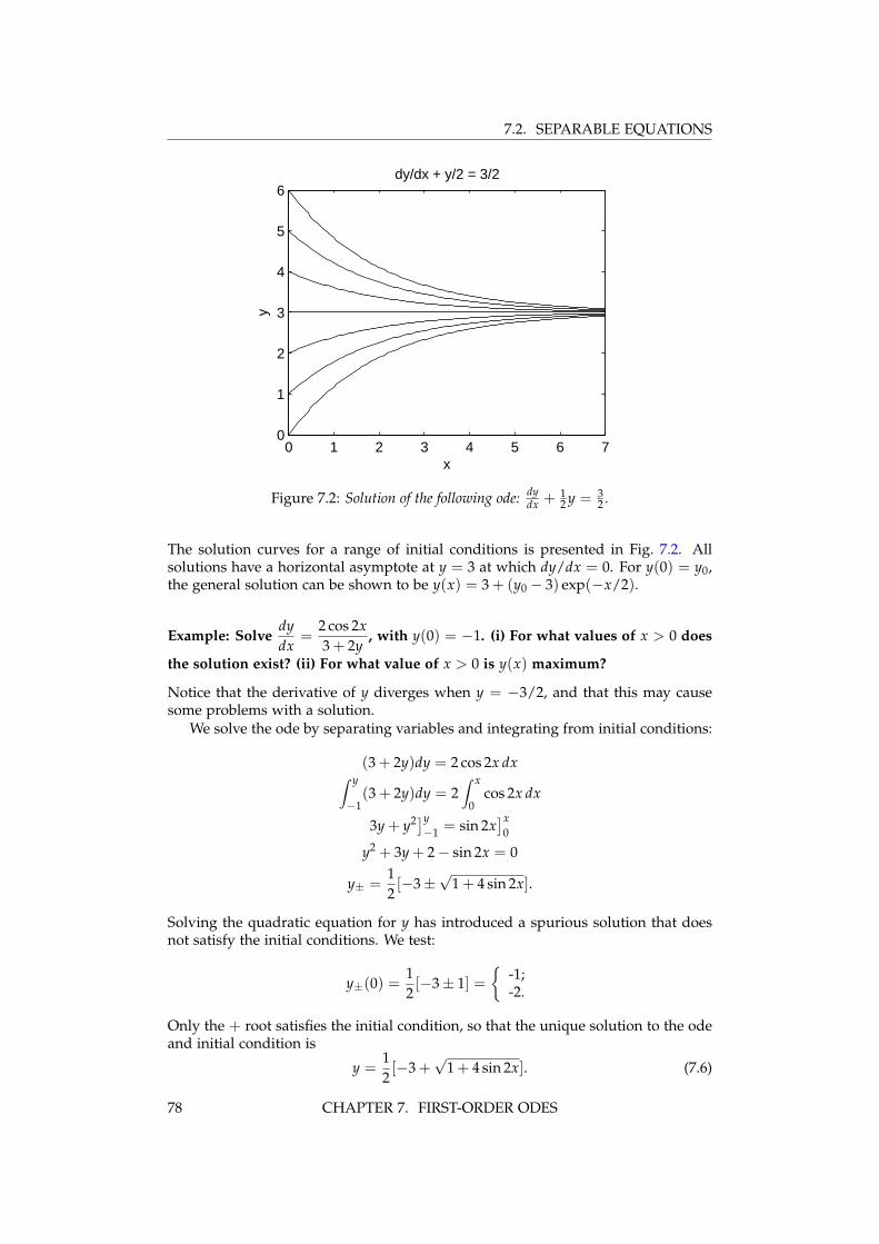
7.2. SEPARABLE EQUATIONS
0 1 2 3 4 5 6 70
1
2
3
4
5
6
x
y
dy/dx + y/2 = 3/2
Figure 7.2: Solution of the following ode: dydx + 1
2 y = 32 .
The solution curves for a range of initial conditions is presented in Fig. 7.2. Allsolutions have a horizontal asymptote at y = 3 at which dy/dx = 0. For y(0) = y0,the general solution can be shown to be y(x) = 3 + (y0 − 3) exp(−x/2).
Example: Solvedydx
=2 cos 2x3 + 2y
, with y(0) = −1. (i) For what values of x > 0 does
the solution exist? (ii) For what value of x > 0 is y(x) maximum?
Notice that the derivative of y diverges when y = −3/2, and that this may causesome problems with a solution.
We solve the ode by separating variables and integrating from initial conditions:
(3 + 2y)dy = 2 cos 2x dx∫ y
−1(3 + 2y)dy = 2
∫ x
0cos 2x dx
3y + y2]y−1 = sin 2x
]x0
y2 + 3y + 2− sin 2x = 0
y± =12[−3±
√1 + 4 sin 2x].
Solving the quadratic equation for y has introduced a spurious solution that doesnot satisfy the initial conditions. We test:
y±(0) =12[−3± 1] =
{-1;-2.
Only the + root satisfies the initial condition, so that the unique solution to the odeand initial condition is
y =12[−3 +
√1 + 4 sin 2x]. (7.6)
78 CHAPTER 7. FIRST-ORDER ODES
7.3. LINEAR EQUATIONS
To determine (i) the values of x > 0 for which the solution exists, we require
1 + 4 sin 2x ≥ 0,
or
sin 2x ≥ −14
. (7.7)
Notice that at x = 0, we have sin 2x = 0; at x = π/4, we have sin 2x = 1; atx = π/2, we have sin 2x = 0; and at x = 3π/4, we have sin 2x = −1 We thereforeneed to determine the value of x such that sin 2x = −1/4, with x in the rangeπ/2 < x < 3π/4. The solution to the ode will then exist for all x between zero andthis value.
To solve sin 2x = −1/4 for x in the interval π/2 < x < 3π/4, one needs torecall the definition of arcsin, or sin−1, as found on a typical scientific calculator.The inverse of the function
f (x) = sin x, −π/2 ≤ x ≤ π/2
is denoted by arcsin. The first solution with x > 0 of the equation sin 2x = −1/4places 2x in the interval (π, 3π/2), so to invert this equation using the arcsinewe need to apply the identity sin (π − x) = sin x, and rewrite sin 2x = −1/4 assin (π − 2x) = −1/4. The solution of this equation may then be found by takingthe arcsine, and is
π − 2x = arcsin (−1/4),
or
x =12
(π + arcsin
14
).
Therefore the solution exists for 0 ≤ x ≤ (π + arcsin (1/4)) /2 = 1.6971 . . . , wherewe have used a calculator value (computing in radians) to find arcsin(0.25) =0.2527 . . . . At the value (x, y) = (1.6971 . . . ,−3/2), the solution curve ends anddy/dx becomes infinite.
To determine (ii) the value of x at which y = y(x) is maximum, we examine(7.6) directly. The value of y will be maximum when sin 2x takes its maximumvalue over the interval where the solution exists. This will be when 2x = π/2, orx = π/4 = 0.7854 . . . .
The graph of y = y(x) is shown in Fig. 7.3.
7.3 Linear equations
View tutorial on YouTube
The linear first-order differential equation (linear in y and its derivative) can bewritten in the form
dydx
+ p(x)y = g(x), (7.8)
with the initial condition y(x0) = y0. Linear first-order equations can be integratedusing an integrating factor µ(x). We multiply (7.8) by µ(x),
µ(x)[
dydx
+ p(x)y]= µ(x)g(x), (7.9)
CHAPTER 7. FIRST-ORDER ODES 79
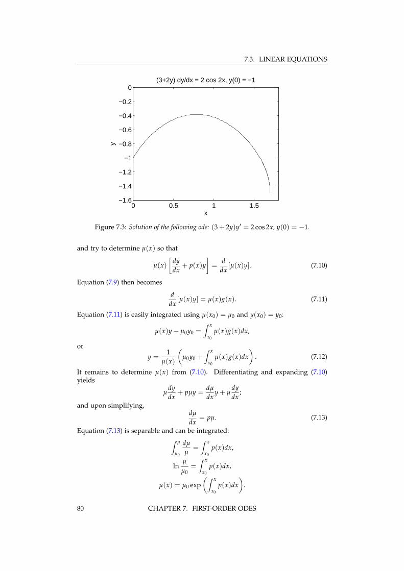
7.3. LINEAR EQUATIONS
0 0.5 1 1.5−1.6
−1.4
−1.2
−1
−0.8
−0.6
−0.4
−0.2
0
x
y
(3+2y) dy/dx = 2 cos 2x, y(0) = −1
Figure 7.3: Solution of the following ode: (3 + 2y)y′ = 2 cos 2x, y(0) = −1.
and try to determine µ(x) so that
µ(x)[
dydx
+ p(x)y]=
ddx
[µ(x)y]. (7.10)
Equation (7.9) then becomes
ddx
[µ(x)y] = µ(x)g(x). (7.11)
Equation (7.11) is easily integrated using µ(x0) = µ0 and y(x0) = y0:
µ(x)y− µ0y0 =∫ x
x0
µ(x)g(x)dx,
or
y =1
µ(x)
(µ0y0 +
∫ x
x0
µ(x)g(x)dx)
. (7.12)
It remains to determine µ(x) from (7.10). Differentiating and expanding (7.10)yields
µdydx
+ pµy =dµ
dxy + µ
dydx
;
and upon simplifying,dµ
dx= pµ. (7.13)
Equation (7.13) is separable and can be integrated:∫ µ
µ0
dµ
µ=∫ x
x0
p(x)dx,
lnµ
µ0=∫ x
x0
p(x)dx,
µ(x) = µ0 exp(∫ x
x0
p(x)dx)
.
80 CHAPTER 7. FIRST-ORDER ODES
7.3. LINEAR EQUATIONS
Notice that since µ0 cancels out of (7.12), it is customary to assign µ0 = 1. Thesolution to (7.8) satisfying the initial condition y(x0) = y0 is then commonly writtenas
y =1
µ(x)
(y0 +
∫ x
x0
µ(x)g(x)dx)
,
with
µ(x) = exp(∫ x
x0
p(x)dx)
the integrating factor. This important result finds frequent use in applied mathe-matics.
Example: Solve dydx + 2y = e−x, with y(0) = 3/4.
Note that this equation is not separable. With p(x) = 2 and g(x) = e−x, we have
µ(x) = exp(∫ x
02dx
)= e2x,
and
y = e−2x(
34+∫ x
0e2xe−xdx
)= e−2x
(34+∫ x
0exdx
)= e−2x
(34+ (ex − 1)
)= e−2x
(ex − 1
4
)= e−x
(1− 1
4e−x)
.
Example: Solve dydx − 2xy = x, with y(0) = 0.
This equation is separable, and we solve it in two ways. First, using an integratingfactor with p(x) = −2x and g(x) = x:
µ(x) = exp(−2
∫ x
0xdx
)= e−x2
,
andy = ex2
∫ x
0xe−x2
dx.
The integral can be done by substitution with u = x2, du = 2xdx:∫ x
0xe−x2
dx =12
∫ x2
0e−udu
= −12
e−u]x2
0
=12
(1− e−x2
).
CHAPTER 7. FIRST-ORDER ODES 81
7.4. APPLICATIONS
Therefore,
y =12
ex2(
1− e−x2)
=12
(ex2 − 1
).
Second, we integrate by separating variables:
dydx− 2xy = x,
dydx
= x(1 + 2y),∫ y
0
dy1 + 2y
=∫ x
0xdx,
12
ln (1 + 2y) =12
x2,
1 + 2y = ex2,
y =12
(ex2 − 1
).
The results from the two different solution methods are the same, and the choice ofmethod is a personal preference.
7.4 Applications
7.4.1 Compound interestView tutorial on YouTube
The equation for the growth of an investment with continuous compounding ofinterest is a first-order differential equation. Let S(t) be the value of the investmentat time t, and let r be the annual interest rate compounded after every time interval∆t. We can also include deposits (or withdrawals). Let k be the annual depositamount, and suppose that an installment is deposited after every time interval ∆t.The value of the investment at the time t + ∆t is then given by
S(t + ∆t) = S(t) + (r∆t)S(t) + k∆t, (7.14)
where at the end of the time interval ∆t, r∆tS(t) is the amount of interest creditedand k∆t is the amount of money deposited (k > 0) or withdrawn (k < 0). As anumerical example, if the account held $10,000 at time t, and r = 6% per year andk = $12,000 per year, say, and the compounding and deposit period is ∆t = 1 month= 1/12 year, then the interest awarded after one month is r∆tS = (0.06/12) ×$10,000 = $50, and the amount deposited is k∆t = $1000.
Rearranging the terms of (7.14) to exhibit what will soon become a derivative,we have
S(t + ∆t)− S(t)∆t
= rS(t) + k.
The equation for continuous compounding of interest and continuous deposits isobtained by taking the limit ∆t→ 0. The resulting differential equation is
dSdt
= rS + k, (7.15)
82 CHAPTER 7. FIRST-ORDER ODES
7.4. APPLICATIONS
which can solved with the initial condition S(0) = S0, where S0 is the initial capital.We can solve either by separating variables or by using an integrating factor; I solvehere by separating variables. Integrating from t = 0 to a final time t,∫ S
S0
dSrS + k
=∫ t
0dt,
1r
ln(
rS + krS0 + k
)= t,
rS + k = (rS0 + k)ert,
S =rS0ert + kert − k
r,
S = S0ert +kr
ert (1− e−rt) , (7.16)
where the first term on the right-hand side of (7.16) comes from the initial investedcapital, and the second term comes from the deposits (or withdrawals). Evidently,compounding results in the exponential growth of an investment.
As a practical example, we can analyze a simple retirement plan. It is easiest toassume that all amounts and returns are in real dollars (adjusted for inflation).Suppose a 25 year-old plans to set aside a fixed amount every year of his/herworking life, invests at a real return of 6%, and retires at age 65. How much musthe/she invest each year to have HK$8,000,000 at retirement? (Note: 1 US$≈ 8 HK$.)We need to solve (7.16) for k using t = 40 years, S(t) = $8,000,000, S0 = 0, andr = 0.06 per year. We have
k =rS(t)
ert − 1,
k =0.06× 8,000,000
e0.06×40 − 1,
= $47,889 year−1.
To have saved approximately one million US$ at retirement, the worker would needto save about HK$50,000 per year over his/her working life. Note that the amountsaved over the worker’s life is approximately 40× $50,000 = $2,000,000, while theamount earned on the investment (at the assumed 6% real return) is approximately$8,000,000− $2,000,000 = $6,000,000. The amount earned from the investment isabout 3× the amount saved, even with the modest real return of 6%. Sound invest-ment planning is well worth the effort.
7.4.2 Chemical reactionsSuppose that two chemicals A and B react to form a product C, which we write as
A + B k→ C,
where k is called the rate constant of the reaction. For simplicity, we will use thesame symbol C, say, to refer to both the chemical C and its concentration. The lawof mass action says that dC/dt is proportional to the product of the concentrationsA and B, with proportionality constant k; that is,
dCdt
= kAB. (7.17)
CHAPTER 7. FIRST-ORDER ODES 83
7.4. APPLICATIONS
Similarly, the law of mass action enables us to write equations for the time-derivativesof the reactant concentrations A and B:
dAdt
= −kAB,dBdt
= −kAB. (7.18)
The ode given by (7.17) can be solved analytically using conservation laws. Weassume that A0 and B0 are the initial concentrations of the reactants, and that noproduct is initially present. From (7.17) and (7.18),
ddt(A + C) = 0 =⇒ A + C = A0,
ddt(B + C) = 0 =⇒ B + C = B0.
Using these conservation laws, (7.17) becomes
dCdt
= k(A0 − C)(B0 − C), C(0) = 0,
which is a nonlinear equation that may be integrated by separating variables. Sep-arating and integrating, we obtain∫ C
0
dC(A0 − C)(B0 − C)
= k∫ t
0dt
= kt. (7.19)
The remaining integral can be done using the method of partial fractions. We write
1(A0 − C)(B0 − C)
=a
A0 − C+
bB0 − C
. (7.20)
The cover-up method is the simplest method to determine the unknown coefficientsa and b. To determine a, we multiply both sides of (7.20) by A0 − C and set C = A0to find
a =1
B0 − A0.
Similarly, to determine b, we multiply both sides of (7.20) by B0 − C and set C = B0to find
b =1
A0 − B0.
Therefore,1
(A0 − C)(B0 − C)=
1B0 − A0
(1
A0 − C− 1
B0 − C
),
and the remaining integral of (7.19) becomes (using C < A0, B0)∫ C
0
dC(A0 − C)(B0 − C)
=1
B0 − A0
(∫ C
0
dCA0 − C
−∫ C
0
dCB0 − C
)=
1B0 − A0
(− ln
(A0 − C
A0
)+ ln
(B0 − C
B0
))=
1B0 − A0
ln(
A0(B0 − C)B0(A0 − C)
).
84 CHAPTER 7. FIRST-ORDER ODES

7.4. APPLICATIONS
Using this integral in (7.19), multiplying by (B0−A0) and exponentiating, we obtain
A0(B0 − C)B0(A0 − C)
= e(B0−A0)kt.
Solving for C, we finally obtain
C(t) = A0B0e(B0−A0)kt − 1
B0e(B0−A0)kt − A0,
which appears to be a complicated expression, but has the simple limits
limt→∞
C(t) =
{A0, if A0 < B0,B0, if B0 < A0
= min(A0, B0).
As one would expect, the reaction stops after one of the reactants is depleted; andthe final concentration of product is equal to the initial concentration of the depletedreactant.
7.4.3 Terminal velocityView tutorial on YouTube
Using Newton’s law, we model a mass m free falling under gravity but with airresistance. We assume that the force of air resistance is proportional to the speedof the mass and opposes the direction of motion. We define the x-axis to pointin the upward direction, opposite the force of gravity. Near the surface of theEarth, the force of gravity is approximately constant and is given by −mg, withg = 9.8 m/s2 the usual gravitational acceleration. The force of air resistance ismodeled by −kv, where v is the vertical velocity of the mass and k is a positiveconstant. When the mass is falling, v < 0 and the force of air resistance is positive,pointing upward and opposing the motion. The total force on the mass is thereforegiven by F = −mg − kv. With F = ma and a = dv/dt, we obtain the differentialequation
mdvdt
= −mg− kv. (7.21)
The terminal velocity v∞ of the mass is defined as the asymptotic velocity after airresistance balances the gravitational force. When the mass is at terminal velocity,dv/dt = 0 so that
v∞ = −mgk
. (7.22)
The approach to the terminal velocity of a mass initially at rest is obtained bysolving (7.21) with initial condition v(0) = 0. The equation is both linear andseparable, and I solve by separating variables:
m∫ v
0
dvmg + kv
= −∫ t
0dt,
mk
ln(
mg + kvmg
)= −t,
1 +kvmg
= e−kt/m,
v = −mgk
(1− e−kt/m
).
CHAPTER 7. FIRST-ORDER ODES 85
7.4. APPLICATIONS
Therefore, v = v∞
(1− e−kt/m
), and v approaches v∞ as the exponential term de-
cays to zero.As an example, a skydiver of mass m = 100 kg with his parachute closed may
have a terminal velocity of 200 km/hr. With
g = (9.8 m/s2)(10−3 km/m)(60 s/min)2(60 min/hr)2 = 127, 008 km/hr2,
one obtains from (7.22), k = 63, 504 kg/hr. One-half of the terminal velocity for free-fall (100 km/hr) is therefore attained when (1− e−kt/m) = 1/2, or t = m ln 2/k ≈4 sec. Approximately 95% of the terminal velocity (190 km/hr ) is attained after17 sec.
7.4.4 Escape velocityView tutorial on YouTube
An interesting physical problem is to find the smallest initial velocity for a masson the Earth’s surface to escape from the Earth’s gravitational field, the so-calledescape velocity. Newton’s law of universal gravitation asserts that the gravitationalforce between two massive bodies is proportional to the product of the two massesand inversely proportional to the square of the distance between them. For a massm a position x above the surface of the Earth, the force on the mass is given by
F = −GMm
(R + x)2 ,
where M and R are the mass and radius of the Earth and G is the gravitationalconstant. The minus sign means the force on the mass m points in the directionof decreasing x. The approximately constant acceleration g on the Earth’s surfacecorresponds to the absolute value of F/m when x = 0:
g =GMR2 ,
and g ≈ 9.8 m/s2. Newton’s law F = ma for the mass m is thus given by
d2xdt2 = − GM
(R + x)2
= − g(1 + x/R)2 , (7.23)
where the radius of the Earth is known to be R ≈ 6350 km.A useful trick allows us to solve this second-order differential equation as a
first-order equation. First, note that d2x/dt2 = dv/dt. If we write v(t) = v(x(t))—considering the velocity of the mass m to be a function of its distance above theEarth—we have using the chain rule
dvdt
=dvdx
dxdt
= vdvdx
,
where we have used v = dx/dt. Therefore, (7.23) becomes the first-order ode
vdvdx
= − g(1 + x/R)2 ,
86 CHAPTER 7. FIRST-ORDER ODES
7.4. APPLICATIONS
which may be solved assuming an initial velocity v(x = 0) = v0 when the mass isshot vertically from the Earth’s surface. Separating variables and integrating, weobtain ∫ v
v0
vdv = −g∫ x
0
dx(1 + x/R)2 .
The left integral is 12 (v
2 − v20), and the right integral can be performed using the
substitution u = 1 + x/R, du = dx/R:∫ x
0
dx(1 + x/R)2 = R
∫ 1+x/R
1
duu2
= − Ru
]1+x/R
1
= R− R2
x + R
=Rx
x + R.
Therefore,12(v2 − v2
0) = −gRx
x + R,
which when multiplied by m is an expression of the conservation of energy (thechange of the kinetic energy of the mass is equal to the change in the potentialenergy). Solving for v2,
v2 = v20 −
2gRxx + R
.
The escape velocity is defined as the minimum initial velocity v0 such that themass can escape to infinity. Therefore, v0 = vescape when v → 0 as x → ∞. Takingthis limit, we have
v2escape = lim
x→∞
2gRxx + R
= 2gR.
With R ≈ 6350 km and g = 127 008 km/hr2, we determine vescape =√
2gR ≈ 40 000km/hr. In comparison, the muzzle velocity of a modern high-performance rifle is4300 km/hr, almost an order of magnitude too slow for a bullet, shot into the sky,to escape the Earth’s gravity.
7.4.5 RC circuit
View tutorial on YouTube
Consider a resister R and a capacitor C connected in series as shown in Fig. 7.4.A battery providing an electromotive force, or emf E , connects to this circuit by aswitch. Initially, there is no charge on the capacitor. When the switch is thrown toa, the battery connects and the capacitor charges. When the switch is thrown to b,the battery disconnects and the capacitor discharges, with energy dissipated in theresister. Here, we determine the voltage drop across the capacitor during chargingand discharging.
CHAPTER 7. FIRST-ORDER ODES 87

7.4. APPLICATIONS
C
R
i
+
_
(a)
(b)
Figure 7.4: RC circuit diagram.
The equations for the voltage drops across a capacitor and a resister are givenby
VC = q/C, VR = iR, (7.24)
where C is the capacitance and R is the resistance. The charge q and the current iare related by
i =dqdt
. (7.25)
Kirchhoff’s voltage law states that the emf E in any closed loop is equal to thesum of the voltage drops in that loop. Applying Kirchhoff’s voltage law when theswitch is thrown to a results in
VR + VC = E . (7.26)
Using (7.24) and (7.25), the voltage drop across the resister can be written in termsof the voltage drop across the capacitor as
VR = RCdVCdt
,
and (7.26) can be rewritten to yield the linear first-order differential equation for VCgiven by
dVCdt
+ VC/RC = E/RC, (7.27)
with initial condition VC(0) = 0.The integrating factor for this equation is
µ(t) = et/RC,
and (7.27) integrates to
VC(t) = e−t/RC∫ t
0(E/RC)et/RCdt,
with solutionVC(t) = E
(1− e−t/RC
).
88 CHAPTER 7. FIRST-ORDER ODES
7.4. APPLICATIONS
The voltage starts at zero and rises exponentially to E , with characteristic time scalegiven by RC.
When the switch is thrown to b, application of Kirchhoff’s voltage law results in
VR + VC = 0,
with corresponding differential equation
dVCdt
+ VC/RC = 0.
Here, we assume that the capacitance is initially fully charged so that VC(0) = E .The solution, then, during the discharge phase is given by
VC(t) = E e−t/RC.
The voltage starts at E and decays exponentially to zero, again with characteristictime scale given by RC.
7.4.6 The logistic equationView tutorial on YouTube
Let N(t) be the number of individuals in a population at time t, and let b and d bethe average per capita birth rate and death rate, respectively. In a short time ∆t, thenumber of births in the population is b∆tN, and the number of deaths is d∆tN. Anequation for N at time t + ∆t is then determined to be
N(t + ∆t) = N(t) + b∆tN(t)− d∆tN(t),
which can be rearranged to
N(t + ∆t)− N(t)∆t
= (b− d)N(t);
and as ∆t→ 0, and with r = b− d, we have
dNdt
= rN.
This is the Malthusian growth model (Thomas Malthus, 1766-1834), and is the sameequation as our compound interest model.
Under a Malthusian growth model, the population size grows exponentially like
N(t) = N0ert,
where N0 is the initial population size. However, when the population growth isconstrained by limited resources, a heuristic modification to the Malthusian growthmodel results in the Verhulst equation,
dNdt
= rN(
1− NK
), (7.28)
where K is called the carrying capacity of the environment. Making (7.28) dimen-sionless using τ = rt and x = N/K leads to the logistic equation,
dxdτ
= x(1− x),
CHAPTER 7. FIRST-ORDER ODES 89

7.4. APPLICATIONS
where we may assume the initial condition x(0) = x0 > 0. Separating variables andintegrating ∫ x
x0
dxx(1− x)
=∫ τ
0dτ.
The integral on the left-hand-side can be done using the method of partial fractions:
1x(1− x)
=ax+
b1− x
,
and the cover-up method yields a = b = 1. Therefore,∫ x
x0
dxx(1− x)
=∫ x
x0
dxx
+∫ x
x0
dx(1− x)
= lnxx0− ln
1− x1− x0
= lnx(1− x0)
x0(1− x)= τ.
Solving for x, we first exponentiate both sides and then isolate x:
x(1− x0)
x0(1− x)= eτ ,
x(1− x0) = x0eτ − xx0eτ ,x(1− x0 + x0eτ) = x0eτ ,
x =x0
x0 + (1− x0)e−τ. (7.29)
We observe that for x0 > 0, we have limτ→∞ x(τ) = 1, corresponding to
limt→∞
N(t) = K.
The population, therefore, grows in size until it reaches the carrying capacity of itsenvironment.
90 CHAPTER 7. FIRST-ORDER ODES

Chapter 8
Linear second-order differentialequations with constantcoefficients
Reference: Boyce and DiPrima, Chapter 3
The general linear second-order differential equation with independent variable tand dependent variable x = x(t) is given by
x + p(t)x + q(t)x = g(t), (8.1)
where we have used the standard physics notation x = dx/dt and x = d2x/dt2.Herein, we assume that p(t) and q(t) are continuous functions on the time intervalfor which we solve (8.1). A unique solution of (8.1) requires initial values x(t0) = x0and x(t0) = u0. The equation with constant coefficients—on which we will devoteconsiderable effort—assumes that p(t) and q(t) are constants, independent of time.The linear second-order ode is said to be homogeneous if g(t) = 0.
8.1 The Euler method
View tutorial on YouTube
In general, (8.1) cannot be solved analytically, and we begin by deriving an algo-rithm for numerical solution. Consider the general second-order ode given by
x = f (t, x, x).
We can write this second-order ode as a pair of first-order odes by defining u = x,and writing the first-order system as
x = u, (8.2)u = f (t, x, u). (8.3)
The first ode, (8.2), gives the slope of the tangent line to the curve x = x(t); thesecond ode, (8.3), gives the slope of the tangent line to the curve u = u(t). Beginningat the initial values (x, u) = (x0, u0) at the time t = t0, we move along the tangentlines to determine x1 = x(t0 + ∆t) and u1 = u(t0 + ∆t):
x1 = x0 + ∆tu0,u1 = u0 + ∆t f (t0, x0, u0).
The values x1 and u1 at the time t1 = t0 + ∆t are then used as new initial valuesto march the solution forward to time t2 = t1 + ∆t. As long as f (t, x, u) is a well-behaved function, the numerical solution converges to the unique solution of theode as ∆t→ 0.
91
8.2. THE PRINCIPLE OF SUPERPOSITION
8.2 The principle of superposition
View tutorial on YouTube
Consider the homogeneous linear second-order ode:
x + p(t)x + q(t)x = 0; (8.4)
and suppose that x = X1(t) and x = X2(t) are solutions to (8.4). We consider alinear combination of X1 and X2 by letting
X(t) = c1X1(t) + c2X2(t), (8.5)
with c1 and c2 constants. The principle of superposition states that x = X(t) is also asolution of (8.4). To prove this, we compute
X + pX + qX = c1X1 + c2X2 + p(c1X1 + c2X2
)+ q (c1X1 + c2X2)
= c1(X1 + pX1 + qX1
)+ c2
(X2 + pX2 + qX2
)= c1 × 0 + c2 × 0= 0,
since X1 and X2 were assumed to be solutions of (8.4). We have therefore shownthat any linear combination of solutions to the homogeneous linear second-orderode is also a solution.
8.3 The Wronskian
View tutorial on YouTube
Suppose that having determined that two solutions of (8.4) are x = X1(t) andx = X2(t), we attempt to write the general solution to (8.4) as (8.5). We must thenask whether this general solution will be able to satisfy two initial conditions givenby
x(t0) = x0, x(t0) = u0, (8.6)
for any initial time t0, and initial values x0 and u0. Applying these initial conditionsto (8.5), we obtain
c1X1(t0) + c2X2(t0) = x0,
c1X1(t0) + c2X2(t0) = u0, (8.7)
which is a system of two linear equations for the two unknowns c1 and c2. In matrixform, (
X1(t0) X2(t0)X1(t0) X2(t0)
)(c1c2
)=
(x0u0
). (8.8)
We can solve (8.8) for any specified values of t0, x0 and u0 if the 2-by-2 matrix isinvertible, and that will be the case if its determinant is nonzero. The determinantis called the Wronskian and is defined by
W = X1X2 − X1X2. (8.9)
92 CHAPTER 8. SECOND-ORDER ODES, CONSTANT COEFFICIENTS

8.4. HOMOGENEOUS ODES
In the language of linear algebra, when W 6= 0 the functions X1 = X1(t) andX2 = X2(t) are linearly independent and span the solution space of the second-order linear differential equation given by (8.4). The solution space of the odesatisfies the conditions of a vector space and the two solutions X1 and X2 act asbasis vectors for this space. The dimension of this space is two, corresponding tothe order of the differential equation.Example: Show that the functions X1(t) = cos ωt and X2(t) = sin ωt have anonzero Wronskian when ω 6= 0.We have
X1(t) = cos ωt, X2(t) = sin ωt
X1(t) = −ω sin ωt, X2(t) = ω cos ωt.
The Wronskian is given by
W =
∣∣∣∣ cos ωt sin ωt−ω sin ωt ω cos ωt
∣∣∣∣ = ω(cos2 ωt + sin2 ωt) = ω,
so that W 6= 0 when ω 6= 0.Example: Show that the functions X1(t) = eat and X2(t) = ebt have a nonzeroWronskian when a 6= b.We have
X1(t) = eat, X2(t) = ebt
X1(t) = aeat, X2(t) = bebt.
The Wronskian is given by
W =
∣∣∣∣ eat ebt
aeat bebt
∣∣∣∣ = (b− a)e(a+b)t,
so that W 6= 0 when a 6= b.Example: Show that the functions X1(t) = 1 and X2(t) = t have a nonzero Wron-skian.We have
X1(t) = 1, X2(t) = t
X1(t) = 0, X2(t) = 1.
The Wronskian is given by
W =
∣∣∣∣1 t0 1
∣∣∣∣ = 1.
8.4 Homogeneous linear second-order ode with con-stant coefficients
View tutorial on YouTube
We now study solutions of the homogeneous, constant coefficient ode, written as
ax + bx + cx = 0, (8.10)
CHAPTER 8. SECOND-ORDER ODES, CONSTANT COEFFICIENTS 93
8.4. HOMOGENEOUS ODES
with a, b, and c constants. Such an equation arises for the charge on a capacitorin an unpowered RLC electrical circuit, or for the position of a freely-oscillatingfrictional mass on a spring, or for a damped pendulum. Our solution method findstwo linearly independent solutions to (8.10), multiplies each of these solutions bya constant, and adds them. The two free constants can then be used to satisfy twogiven initial conditions.
Because of the differential properties of the exponential function, a naturalansatz, or educated guess, for the form of the solution to (8.10) is x = ert, wherer is a constant to be determined. Successive differentiation results in x = rert andx = r2ert, and substitution into (8.10) yields
ar2ert + brert + cert = 0. (8.11)
Our choice of exponential function is now rewarded by the explicit cancelation in(8.11) of ert. The result is a quadratic equation for the unknown constant r:
ar2 + br + c = 0. (8.12)
Our ansatz has thus converted a differential equation into an algebraic equation.Equation (8.12) is called the characteristic equation of (8.10). Using the quadraticformula, the two solutions of the characteristic equation (8.12) are given by
r± =12a
(−b±
√b2 − 4ac
).
There are three cases to consider: (1) if b2 − 4ac > 0, then the two roots are distinctand real; (2) if b2 − 4ac < 0, then the two roots are complex conjugates (3) if b2 −4ac = 0, then the two roots are degenerate and there is only one real root. We willconsider these three cases in turn.
8.4.1 Distinct real rootsWhen r+ 6= r− are real roots, then the general solution to (8.10) can be written as alinear superposition of the two solutions er+t and er−t; that is,
x(t) = c1er+t + c2er−t.
The unknown constants c1 and c2 can then be determined by the given initial con-ditions x(t0) = x0 and x(t0) = u0. We now present two examples.
Example 1: Solve x + 5x + 6x = 0 with x(0) = 2, x(0) = 3, and find the maximumvalue attained by x.
View tutorial on YouTube
We take as our ansatz x = ert and obtain the characteristic equation
r2 + 5r + 6 = 0,
which factors to(r + 3)(r + 2) = 0.
The general solution to the ode is thus
x(t) = c1e−2t + c2e−3t.
94 CHAPTER 8. SECOND-ORDER ODES, CONSTANT COEFFICIENTS
8.4. HOMOGENEOUS ODES
The solution for x obtained by differentiation is
x(t) = −2c1e−2t − 3c2e−3t.
Use of the initial conditions then results in two equations for the two unknownconstant c1 and c2:
c1 + c2 = 2,−2c1 − 3c2 = 3.
Adding three times the first equation to the second equation yields c1 = 9; and thefirst equation then yields c2 = 2− c1 = −7. Therefore, the unique solution thatsatisfies both the ode and the initial conditions is
x(t) = 9e−2t − 7e−3t
= 9e−2t(
1− 79
e−t)
.
Note that although both exponential terms decay in time, their sum increases ini-tially since x(0) > 0. The maximum value of x occurs at the time tm when x = 0,or
tm = ln (7/6) .
The maximum xm = x(tm) is then determined to be
xm = 108/49.
Example 2: Solve x− x = 0 with x(0) = x0, x(0) = u0.
Again our ansatz is x = ert, and we obtain the characteristic equation
r2 − 1 = 0,
with solution r± = ±1. Therefore, the general solution for x is
x(t) = c1et + c2e−t,
and the derivative satisfiesx(t) = c1et − c2e−t.
Initial conditions are satisfied when
c1 + c2 = x0,c1 − c2 = u0.
Adding and subtracting these equations, we determine
c1 =12(x0 + u0) , c2 =
12(x0 − u0) ,
so that after rearranging terms
x(t) = x0
(et + e−t
2
)+ u0
(et − e−t
2
).
CHAPTER 8. SECOND-ORDER ODES, CONSTANT COEFFICIENTS 95
8.4. HOMOGENEOUS ODES
The terms in parentheses are the usual definitions of the hyperbolic cosine and sinefunctions; that is,
cosh t =et + e−t
2, sinh t =
et − e−t
2.
Our solution can therefore be rewritten as
x(t) = x0 cosh t + u0 sinh t.
Note that the relationships between the trigonometric functions and the complexexponentials were given by
cos t =eit + e−it
2, sin t =
eit − e−it
2i,
so thatcosh t = cos it, sinh t = −i sin it.
Also note that the hyperbolic trigonometric functions satisfy the differential equa-tions
ddt
sinh t = cosh t,ddt
cosh t = sinh t,
which though similar to the differential equations satisfied by the more commonlyused trigonometric functions, is absent a minus sign.
8.4.2 Distinct complex-conjugate rootsView tutorial on YouTube
We now consider a characteristic equation (8.12) with b2 − 4ac < 0, so the rootsoccur as complex conjugate pairs. With
λ = − b2a
, µ =12a
√4ac− b2,
the two roots of the characteristic equation are λ + iµ and λ − iµ. We have thusfound the following two complex exponential solutions to the differential equation:
Z1(t) = eλteiµt, Z2(t) = eλte−iµt.
Applying the principle of superposition, any linear combination of Z1 and Z2 isalso a solution to the second-order ode.
Recall that if z = x + iy, then Re z = (z + z)/2 and Im z = (z− z)/2i. We cantherefore form two different linear combinations of Z1(t) and Z2(t) that are real,namely X1(t) = Re Z1(t) and X2(t) = Im Z1(t). We have
X1(t) = eλt cos µt, X2(t) = eλt sin µt.
Having found these two real solutions, X1(t) and X2(t), we can then apply theprinciple of superposition a second time to determine the general solution for x(t):
x(t) = eλt (A cos µt + B sin µt) . (8.13)
It is best to memorize this result. The real part of the roots of the characteristic equa-tion goes into the exponential function; the imaginary part goes into the argumentof cosine and sine.
96 CHAPTER 8. SECOND-ORDER ODES, CONSTANT COEFFICIENTS
8.4. HOMOGENEOUS ODES
Example 1: Solve x + x = 0 with x(0) = x0 and x(0) = u0.
View tutorial on YouTube
The characteristic equation isr2 + 1 = 0,
with rootsr± = ±i.
The general solution of the ode is therefore
x(t) = A cos t + B sin t.
The derivative isx(t) = −A sin t + B cos t.
Applying the initial conditions:
x(0) = A = x0, x(0) = B = u0;
so that the final solution is
x(t) = x0 cos t + u0 sin t.
Recall that we wrote the analogous solution to the ode x − x = 0 as x(t) =x0 cosh t + u0 sinh t.
Example 2: Solve x + x + x = 0 with x(0) = 1 and x(0) = 0.
The characteristic equation isr2 + r + 1 = 0,
with roots
r± = −12± i√
32
.
The general solution of the ode is therefore
x(t) = e−12 t
(A cos
√3
2t + B sin
√3
2t
).
The derivative is
x(t) = −12
e−12 t
(A cos
√3
2t + B sin
√3
2t
)
+
√3
2e−
12 t
(−A sin
√3
2t + B cos
√3
2t
).
Applying the initial conditions x(0) = 1 and x(0) = 0:
A = 1,
−12
A +
√3
2B = 0;
CHAPTER 8. SECOND-ORDER ODES, CONSTANT COEFFICIENTS 97
8.4. HOMOGENEOUS ODES
or
A = 1, B =
√3
3.
Therefore,
x(t) = e−12 t
(cos
√3
2t +√
33
sin
√3
2t
).
8.4.3 Degenerate rootsView tutorial on YouTube
Finally, we consider the characteristic equation,
ar2 + br + c = 0,
with b2 − 4ac = 0. The degenerate root is then given by
r = − b2a
,
yielding only a single solution to the ode:
x1(t) = exp(− bt
2a
). (8.14)
To satisfy two initial conditions, a second independent solution must be found withnonzero Wronskian, and apparently this second solution is not of the form of ouransatz x = exp (rt).
One method to determine this missing second solution is to try the ansatz
x(t) = y(t)x1(t), (8.15)
where y(t) is an unknown function that satisfies the differential equation obtainedby substituting (8.15) into (8.10). This standard technique is called the reduction oforder method and enables one to find a second solution of a homogeneous lineardifferential equation if one solution is known. If the original differential equation isof order n, the differential equation for y = y(t) reduces to an order one lower, thatis, n− 1.
Here, however, we will determine this missing second solution through a lim-iting process. We start with the solution obtained for complex roots of the charac-teristic equation, and then arrive at the solution obtained for degenerate roots bytaking the limit µ→ 0.
Now, the general solution for complex roots was given by (8.13), and to properlylimit this solution as µ → 0 requires first satisfying the specific initial conditionsx(0) = x0 and x(0) = u0. Solving for A and B, the general solution given by (8.13)becomes the specific solution
x(t; µ) = eλt(
x0 cos µt +u0 − λx0
µsin µt
).
Here, we have written x = x(t; µ) to show explicitly that x depends on µ.Taking the limit as µ→ 0, and using limµ→0 µ−1 sin µt = t, we have
limµ→0
x(t; µ) = eλt(x0 + (u0 − λx0)t).
98 CHAPTER 8. SECOND-ORDER ODES, CONSTANT COEFFICIENTS
8.5. DIFFERENCE EQUATIONS
The second solution is observed to be a constant, u0 − λx0, times t times the firstsolution, eλt. Our general solution to the ode (8.10) when b2− 4ac = 0 can thereforebe written in the form
x(t) = (c1 + c2t)ert,
where r is the repeated root of the characteristic equation. The main result to beremembered is that for the case of repeated roots, the second solution is t times thefirst solution.
Example: Solve x + 2x + x = 0 with x(0) = 1 and x(0) = 0.
The characteristic equation is
r2 + 2r + 1 = (r + 1)2
= 0,
which has a repeated root given by r = −1. Therefore, the general solution to theode is
x(t) = c1e−t + c2te−t,
with derivativex(t) = −c1e−t + c2e−t − c2te−t.
Applying the initial conditions, we have
c1 = 1,−c1 + c2 = 0,
so that c1 = c2 = 1. Therefore, the solution is
x(t) = (1 + t)e−t.
8.5 Homogeneous linear second-order difference equa-tions with constant coefficients
The solution of linear difference equations is similar to that of linear differentialequations. Here, we solve one interesting example.Example: Find an explicit formula for the nth Fibonacci number Fn, where
Fn+1 = Fn + Fn−1, F1 = F2 = 1.
This will be our second derivation of Binet’s formula (see §5.2 for the first deriva-tion). We consider the relevant difference equation
xn+1 − xn − xn−1 = 0, (8.16)
and try to solve it using a method similar to the solution of a second-order differ-ential equation. An appropriate ansatz here is
xn = λn, (8.17)
where λ is an unknown constant. Substitution of (8.17) into (8.16) results in
λn+1 − λn − λn−1 = 0,
CHAPTER 8. SECOND-ORDER ODES, CONSTANT COEFFICIENTS 99
8.6. INHOMOGENEOUS ODES
or upon division by λn−1,λ2 − λ− 1 = 0.
Use of the quadratic formula yields two roots. We have
λ1 =1 +√
52
= Φ, λ2 =1−√
52
= −φ,
where Φ is the golden ratio and φ is the golden ratio conjugate.We have thus found two independent solutions to (8.16) of the form (8.17), and
we can now use these two solutions to determine a formula for Fn. Multiplying thesolutions by constants and adding them, we obtain
Fn = c1Φn + c2(−φ)n, (8.18)
which must satisfy the initial values F1 = F2 = 1. The algebra for finding theunknown constants can be made simpler, however, if instead of F2, we use thevalue F0 = F2 − F1 = 0.
Application of the values for F0 and F1 results in the system of equations givenby
c1 + c2 = 0,c1Φ− c2φ = 1.
We use the first equation to write c2 = −c1, and substitute into the second equationto get
c1(Φ + φ) = 1.
Since Φ + φ =√
5, we can solve for c1 and c2 to obtain
c1 = 1/√
5, c2 = −1/√
5. (8.19)
Using (8.19) in (8.18) then derives Binet’s formula
Fn =Φn − (−φ)n√
5. (8.20)
8.6 Inhomogeneous linear second-order ode
We now consider the general inhomogeneous linear second-order ode (8.1):
x + p(t)x + q(t)x = g(t), (8.21)
with initial conditions x(t0) = x0 and x(t0) = u0. There is a three-step solutionmethod when the inhomogeneous term g(t) 6= 0. (i) Find the general solution ofthe homogeneous equation
x + p(t)x + q(t)x = 0. (8.22)
Let us denote the homogeneous solution by
xh(t) = c1X1(t) + c2X2(t),
where X1 and X2 are linearly independent solutions of (8.22), and c1 and c2 areas yet undetermined constants. (ii) Find a particular solution xp of the inhomoge-neous equation (8.21). A particular solution is readily found when p(t) and q(t) are
100 CHAPTER 8. SECOND-ORDER ODES, CONSTANT COEFFICIENTS
8.6. INHOMOGENEOUS ODES
constants, and when g(t) is a combination of polynomials, exponentials, sines andcosines. (iii) Write the general solution of (8.21) as the sum of the homogeneousand particular solutions,
x(t) = xh(t) + xp(t), (8.23)
and apply the initial conditions to determine the constants c1 and c2. Note thatbecause of the linearity of (8.21),
x + px + qx =d2
dt2 (xh + xp) + pddt(xh + xp) + q(xh + xp)
= (xh + pxh + qxh) + (xp + pxp + qxp)
= 0 + g= g,
so that (8.23) solves (8.21), and the two free constants in xh can be used to satisfythe initial conditions.
We will consider here only the constant coefficient case. We now illustrate thesolution method by an example.
Example: Solve x− 3x− 4x = 3e2t with x(0) = 1 and x(0) = 0.
View tutorial on YouTube
First, we solve the homogeneous equation. The characteristic equation is
r2 − 3r− 4 = (r− 4)(r + 1)= 0,
so thatxh(t) = c1e4t + c2e−t.
Second, we find a particular solution of the inhomogeneous equation. The form ofthe particular solution is chosen such that the exponential will cancel out of bothsides of the ode. The ansatz we choose is
x(t) = Ae2t, (8.24)
where A is a yet undetermined coefficient. Upon substituting x into the ode, differ-entiating using the chain rule, and canceling the exponential, we obtain
4A− 6A− 4A = 3,
from which we determine A = −1/2. Obtaining a solution for A independent of tjustifies the ansatz (8.24). Third, we write the general solution to the ode as the sumof the homogeneous and particular solutions, and determine c1 and c2 that satisfythe initial conditions. We have
x(t) = c1e4t + c2e−t − 12
e2t;
and taking the derivative,
x(t) = 4c1e4t − c2e−t − e2t.
CHAPTER 8. SECOND-ORDER ODES, CONSTANT COEFFICIENTS 101

8.6. INHOMOGENEOUS ODES
Applying the initial conditions,
c1 + c2 −12= 1,
4c1 − c2 − 1 = 0;
or
c1 + c2 =32
,
4c1 − c2 = 1.
This system of linear equations can be solved for c1 by adding the equations toobtain c1 = 1/2, after which c2 = 1 can be determined from the first equation.Therefore, the solution for x(t) that satisfies both the ode and the initial conditionsis given by
x(t) =12
e4t − 12
e2t + e−t
=12
e4t(
1− e−2t + 2e−5t)
,
where we have grouped the terms in the solution to better display the asymptoticbehavior for large t.
We now find particular solutions for some relatively simple inhomogeneousterms using this method of undetermined coefficients.
Example: Find a particular solution of x− 3x− 4x = 2 sin t.
View tutorial on YouTube
We show two methods for finding a particular solution. The first more directmethod tries the ansatz
x(t) = A cos t + B sin t,
where the argument of cosine and sine must agree with the argument of sine in theinhomogeneous term. The cosine term is required because the derivative of sine iscosine. Upon substitution into the differential equation, we obtain
(−A cos t− B sin t)− 3 (−A sin t + B cos t)− 4 (A cos t + B sin t) = 2 sin t,
or regrouping terms,
− (5A + 3B) cos t + (3A− 5B) sin t = 2 sin t.
This equation is valid for all t, and in particular for t = 0 and π/2, for which thesine and cosine functions vanish. For these two values of t, we find
5A + 3B = 0, 3A− 5B = 2;
and solving for A and B, we obtain
A =317
, B = − 517
.
102 CHAPTER 8. SECOND-ORDER ODES, CONSTANT COEFFICIENTS
8.6. INHOMOGENEOUS ODES
The particular solution is therefore given by
xp =117
(3 cos t− 5 sin t) .
The second solution method makes use of the relation eit = cos t + i sin t toconvert the sine inhomogeneous term to an exponential function. We introduce thecomplex function z(t) by letting
z(t) = x(t) + iy(t),
and rewrite the differential equation in complex form. We can rewrite the equa-tion in one of two ways. On the one hand, if we use sin t = Re{−ieit}, then thedifferential equation is written as
z− 3z− 4z = −2ieit; (8.25)
and by equating the real and imaginary parts, this equation becomes the two realdifferential equations
x− 3x− 4x = 2 sin t, y− 3y− 4y = −2 cos t.
The solution we are looking for, then, is xp(t) = Re{zp(t)}.On the other hand, if we write sin t = Im{eit}, then the complex differential
equation becomesz− 3z− 4z = 2eit, (8.26)
which becomes the two real differential equations
x− 3x− 4x = 2 cos t, y− 3y− 4y = 2 sin t.
Here, the solution we are looking for is xp(t) = Im{zp(t)}.We will proceed here by solving (8.26). As we now have an exponential function
as the inhomogeneous term, we can make the ansatz
z(t) = Ceit,
where we now expect C to be a complex constant. Upon substitution into the ode(8.26) and using i2 = −1:
−C− 3iC− 4C = 2;
or solving for C:
C =−2
5 + 3i
=−2(5− 3i)
(5 + 3i)(5− 3i)
=−10 + 6i
34
=−5 + 3i
17.
Therefore,
xp = Im{zp}
= Im{
117
(−5 + 3i)(cos t + i sin t)}
=117
(3 cos t− 5 sin t).
CHAPTER 8. SECOND-ORDER ODES, CONSTANT COEFFICIENTS 103

8.7. RESONANCE
Example: Find a particular solution of x + x− 2x = t2.
View tutorial on YouTube
The correct ansatz here is the polynomial
x(t) = At2 + Bt + C.
Upon substitution into the ode, we have
2A + 2At + B− 2At2 − 2Bt− 2C = t2,
or−2At2 + 2(A− B)t + (2A + B− 2C)t0 = t2.
Equating powers of t,
−2A = 1, 2(A− B) = 0, 2A + B− 2C = 0;
and solving,
A = −12
, B = −12
, C = −34
.
The particular solution is therefore
xp(t) = −12
t2 − 12
t− 34
.
8.7 Resonance
View tutorial on YouTube
Resonance occurs when the frequency of the inhomogeneous term matches thefrequency of the homogeneous solution. To illustrate resonance in its simplest em-bodiment, we consider the second-order linear inhomogeneous ode
x + ω20x = f cos ωt, x(0) = x0, x(0) = u0. (8.27)
Our main goal is to determine what happens to the solution in the limit ω → ω0.The homogeneous equation has characteristic equation
r2 + ω20 = 0,
so that r± = ±iω0. Therefore,
xh(t) = c1 cos ω0t + c2 sin ω0t. (8.28)
To find a particular solution, we note the absence of a first-derivative term, andsimply try
x(t) = A cos ωt.
Upon substitution into the ode, we obtain
−ω2 A + ω20 A = f ,
104 CHAPTER 8. SECOND-ORDER ODES, CONSTANT COEFFICIENTS
8.7. RESONANCE
orA =
fω2
0 −ω2.
Therefore,
xp(t) =f
ω20 −ω2
cos ωt.
Our general solution is thus
x(t) = c1 cos ω0t + c2 sin ω0t +f
ω20 −ω2
cos ωt,
with derivative
x(t) = ω0(c2 cos ω0t− c1 sin ω0t)− f ω
ω20 −ω2
sin ωt.
Initial conditions are satisfied when
x0 = c1 +f
ω20 −ω2
,
u0 = c2ω0,
so thatc1 = x0 −
fω2
0 −ω2, c2 =
u0
ω0.
Therefore, the solution to the ode that satisfies the initial conditions is
x(t) =
(x0 −
fω2
0 −ω2
)cos ω0t +
u0
ω0sin ω0t +
fω2
0 −ω2cos ωt
= x0 cos ω0t +u0
ω0sin ω0t +
f (cos ωt− cos ω0t)ω2
0 −ω2,
where we have grouped together terms proportional to the forcing amplitude f .Resonance occurs in the limit ω → ω0; that is, the frequency of the inhomoge-
neous term (the external force) matches the frequency of the homogeneous solution(the free oscillation). By L’Hospital’s rule, the limit of the term proportional to f isfound by differentiating with respect to ω:
limω→ω0
f (cos ωt− cos ω0t)ω2
0 −ω2= lim
ω→ω0
− f t sin ωt−2ω
=f t sin ω0t
2ω0.
(8.29)
At resonance, the term proportional to the amplitude f of the inhomogeneous termincreases linearly with t, resulting in larger-and-larger amplitudes of oscillation forx(t). In general, if the inhomogeneous term in the differential equation is a solutionof the corresponding homogeneous differential equation, then the correct ansatz forthe particular solution is a constant times the inhomogeneous term times t.
To illustrate this same example further, we return to the original ode, now as-sumed to be exactly at resonance,
x + ω20x = f cos ω0t,
CHAPTER 8. SECOND-ORDER ODES, CONSTANT COEFFICIENTS 105
8.7. RESONANCE
and find a particular solution directly. The particular solution is the real part of theparticular solution of
z + ω20z = f eiω0t.
If we try zp = Ceiω0t, we obtain 0 = f , showing that the particular solution is notof this form. Because the inhomogeneous term is a solution of the homogeneousequation, we should take as our ansatz
zp = Ateiω0t.
We havezp = Aeiω0t (1 + iω0t) , zp = Aeiω0t
(2iω0 −ω2
0t)
;
and upon substitution into the ode
zp + ω20zp = Aeiω0t
(2iω0 −ω2
0t)+ ω2
0 Ateiω0t
= 2iω0 Aeiω0t
= f eiω0t.
Therefore,
A =f
2iω0,
and
xp = Re{ f t2iω0
eiω0t}
=f t sin ω0t
2ω0,
the same result as (8.29).
Example: Find a particular solution of x− 3x− 4x = 5e−t .
View tutorial on YouTube
If we naively try the ansatzx = Ae−t,
and substitute this into the inhomogeneous differential equation, we obtain
A + 3A− 4A = 5,
or 0 = 5, which is clearly nonsense. Our ansatz therefore fails to find a solution. Thecause of this failure is that the corresponding homogeneous equation has solution
xh = c1e4t + c2e−t,
so that the inhomogeneous term 5e−t is one of the solutions of the homogeneousequation. To find a particular solution, we should therefore take as our ansatz
x = Ate−t,
with first- and second-derivatives given by
x = Ae−t(1− t), x = Ae−t(−2 + t).
106 CHAPTER 8. SECOND-ORDER ODES, CONSTANT COEFFICIENTS
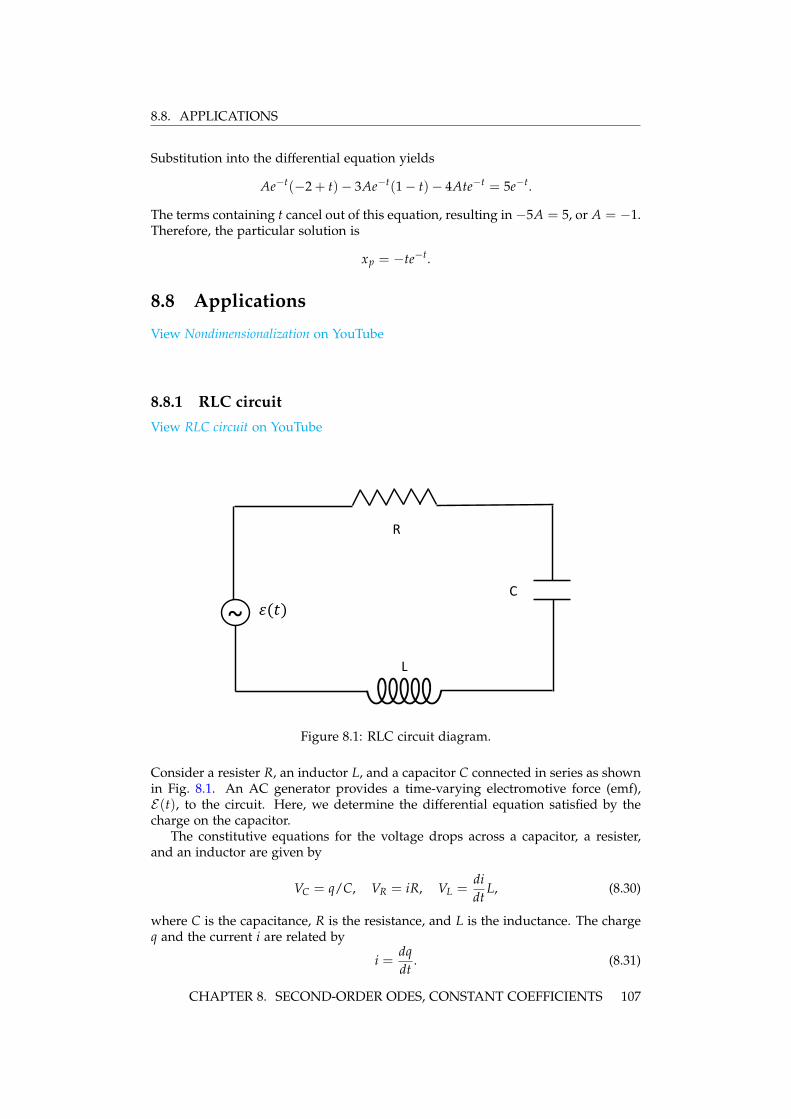
8.8. APPLICATIONS
Substitution into the differential equation yields
Ae−t(−2 + t)− 3Ae−t(1− t)− 4Ate−t = 5e−t.
The terms containing t cancel out of this equation, resulting in −5A = 5, or A = −1.Therefore, the particular solution is
xp = −te−t.
8.8 Applications
View Nondimensionalization on YouTube
8.8.1 RLC circuitView RLC circuit on YouTube
C
𝜀(𝑡)
R
L
~
Figure 8.1: RLC circuit diagram.
Consider a resister R, an inductor L, and a capacitor C connected in series as shownin Fig. 8.1. An AC generator provides a time-varying electromotive force (emf),E(t), to the circuit. Here, we determine the differential equation satisfied by thecharge on the capacitor.
The constitutive equations for the voltage drops across a capacitor, a resister,and an inductor are given by
VC = q/C, VR = iR, VL =didt
L, (8.30)
where C is the capacitance, R is the resistance, and L is the inductance. The chargeq and the current i are related by
i =dqdt
. (8.31)
CHAPTER 8. SECOND-ORDER ODES, CONSTANT COEFFICIENTS 107
8.8. APPLICATIONS
Kirchhoff’s voltage law states that the emf E applied to any closed loop is equalto the sum of the voltage drops in that loop. Applying Kirchhoff’s voltage law tothe RLC ciruit results in
VL + VR + VC = E(t); (8.32)
or using (8.30) and (8.31),
Ld2qdt2 + R
dqdt
+1C
q = E(t).
The equation for the RLC circuit is a second-order linear inhomogeneous differen-tial equation with constant coefficients.
The AC voltage can be written as E(t) = E0 cos ωt, and the governing equationfor q = q(t) can be written as
d2qdt2 +
RL
dqdt
+1
LCq =E0
Lcos ωt. (8.33)
Nondimensionalization of this equation will be shown to reduce the number of freeparameters.
To construct dimensionless variables, we first define the natural frequency ofoscillation of a system to be the frequency of oscillation in the absence of any drivingor damping forces. The iconic example is the simple harmonic oscillator, withequation given by
x + ω20x = 0,
and general solution given by x(t) = A cos ω0t + B sin ω0t. Here, the natural fre-quency of oscillation is ω0, and the period of oscillation is T = 2π/ω0. For theRLC circuit, the natural frequency of oscillation is found from the coefficient of theq term, and is given by
ω0 =1√LC
.
Making use of ω0, with units of one over time, we can define a dimensionless timeτ and a dimensionless charge Q by
τ = ω0t, Q =ω2
0 LE0
q.
The resulting dimensionless equation for the RLC circuit is then given by
d2Qdτ2 + α
dQdτ
+ Q = cos βτ, (8.34)
where α and β are dimensionless parameters given by
α =R
Lω0, β =
ω
ω0.
Notice that the original five parameters in (8.33), namely R, L, C, E0 and ω, havebeen reduced to the two dimensionless parameters α and β. We will return later tosolve (8.34) after visiting two more applications that will be shown to be governedby the same dimensionless equation.
108 CHAPTER 8. SECOND-ORDER ODES, CONSTANT COEFFICIENTS
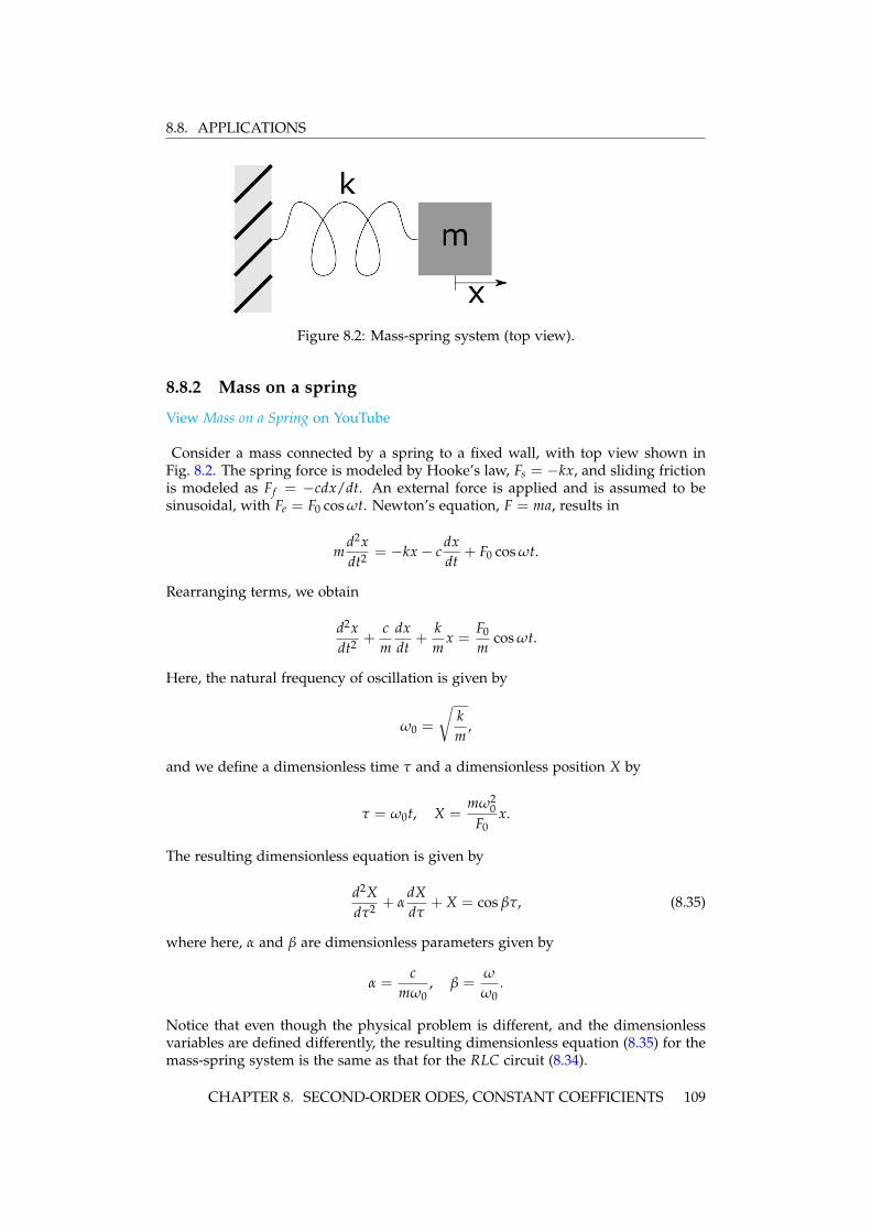
8.8. APPLICATIONS
Figure 8.2: Mass-spring system (top view).
8.8.2 Mass on a spring
View Mass on a Spring on YouTube
Consider a mass connected by a spring to a fixed wall, with top view shown inFig. 8.2. The spring force is modeled by Hooke’s law, Fs = −kx, and sliding frictionis modeled as Ff = −cdx/dt. An external force is applied and is assumed to besinusoidal, with Fe = F0 cos ωt. Newton’s equation, F = ma, results in
md2xdt2 = −kx− c
dxdt
+ F0 cos ωt.
Rearranging terms, we obtain
d2xdt2 +
cm
dxdt
+km
x =F0
mcos ωt.
Here, the natural frequency of oscillation is given by
ω0 =
√km
,
and we define a dimensionless time τ and a dimensionless position X by
τ = ω0t, X =mω2
0F0
x.
The resulting dimensionless equation is given by
d2Xdτ2 + α
dXdτ
+ X = cos βτ, (8.35)
where here, α and β are dimensionless parameters given by
α =c
mω0, β =
ω
ω0.
Notice that even though the physical problem is different, and the dimensionlessvariables are defined differently, the resulting dimensionless equation (8.35) for themass-spring system is the same as that for the RLC circuit (8.34).
CHAPTER 8. SECOND-ORDER ODES, CONSTANT COEFFICIENTS 109
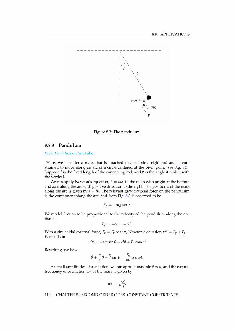
8.8. APPLICATIONS
mg
mg sin θ
θ
l
θ
Figure 8.3: The pendulum.
8.8.3 Pendulum
View Pendulum on YouTube
Here, we consider a mass that is attached to a massless rigid rod and is con-strained to move along an arc of a circle centered at the pivot point (see Fig. 8.3).Suppose l is the fixed length of the connecting rod, and θ is the angle it makes withthe vertical.
We can apply Newton’s equation, F = ma, to the mass with origin at the bottomand axis along the arc with positive direction to the right. The position s of the massalong the arc is given by s = lθ. The relevant gravitrational force on the pendulumis the component along the arc, and from Fig. 8.3 is observed to be
Fg = −mg sin θ.
We model friction to be proportional to the velocity of the pendulum along the arc,that is
Ff = −cs = −clθ.
With a sinusoidal external force, Fe = F0 cos ωt, Newton’s equation ms = Fg + Ff +Fe results in
mlθ = −mg sin θ − clθ + F0 cos ωt.
Rewriting, we have
θ +cm
θ +gl
sin θ =F0
mlcos ωt.
At small amplitudes of oscillation, we can approximate sin θ ≈ θ, and the naturalfrequency of oscillation ω0 of the mass is given by
ω0 =
√gl
.
110 CHAPTER 8. SECOND-ORDER ODES, CONSTANT COEFFICIENTS
8.9. DAMPED RESONANCE
Nondimensionalizing time as τ = ω0t, the dimensionless pendulum equation be-comes
d2θ
dτ2 + αdθ
dτ+ sin θ = γ cos βτ,
where α, β, and γ are dimensionless parameters given by
α =c
mω0, β =
ω
ω0, γ =
F0
mlω20
.
The nonlinearity of the pendulum equation, with the term sin θ, results in the addi-tional dimensionless parameter γ. For small amplitude of oscillation, however, wecan scale θ by θ = γΘ, and the small amplitude dimensionless equation becomes
d2Θdτ2 + α
dΘdτ
+ Θ = cos βτ, (8.36)
the same equation as (8.34) and (8.35).
8.9 Damped resonance
View Damped Resonance on YouTube
We now solve the dimensionless equations given by (8.34), (8.35) and (8.36), writtenhere as
x + αx + x = cos βt, (8.37)
where the physical constraints of our three applications requires that α > 0. Thehomogeneous equation has characteristic equation
r2 + αr + 1 = 0,
so that the solutions are
r± = −α
2± 1
2
√α2 − 4.
When α2 − 4 < 0, the motion of the unforced oscillator is said to be underdamped;when α2 − 4 > 0, overdamped; and when α2 − 4 = 0, critically damped. For allthree types of damping, the roots of the characteristic equation satisfy Re(r±) < 0.Therefore, both linearly independent homogeneous solutions decay exponentiallyto zero, and the long-time asymptotic solution of (8.37) reduces to the non-decayingparticular solution. Since the initial conditions are satisfied by the free constantsmultiplying the decaying homogeneous solutions, the long-time asymptotic solu-tion is independent of the initial conditions.
If we are only interested in the long-time asymptotic solution of (8.37), we canproceed directly to the determination of a particular solution. As before, we con-sider the complex ode
z + αz + z = eiβt,
with xp = Re(zp). With the ansatz zp = Aeiβt, we have
−β2 A + iαβA + A = 1,
CHAPTER 8. SECOND-ORDER ODES, CONSTANT COEFFICIENTS 111
8.9. DAMPED RESONANCE
or
A =1
(1− β2) + iαβ
=
(1
(1− β2)2 + α2β2
)((1− β2)− iαβ
).
(8.38)
To determine xp, we utilize the polar form of a complex number. The complexnumber z = x + iy can be written in polar form as z = reiφ, where r =
√x2 + y2
and tan φ = y/x. We therefore write
(1− β2)− iαβ = reiφ,
withr =
√(1− β2)2 + α2β2, tan φ = − αβ
1− β2 .
Using the polar form, A in (8.38) becomes
A =
(1√
(1− β2)2 + α2β2
)eiφ,
and xp = Re(Aeiβt) becomes
xp =
(1√
(1− β2)2 + α2β2
)Re{
ei(βt+φ)}
=
(1√
(1− β2)2 + α2β2
)cos (βt + φ).
(8.39)
We conclude with a couple of observations about (8.39). First, if the forcingfrequency ω is equal to the natural frequency ω0 of the undamped oscillator, thenβ = 1 and A = 1/iα, and xp = (1/α) sin t. The oscillator position is observedto be π/2 out of phase with the external force, or in other words, the velocity ofthe oscillator, not the position, is in phase with the force. Second, the value of βthat maximizes the amplitude of oscillation is the value of β that minimizes thedenominator of (8.39). To determine βm we thus minimize the function g(β2) withrespect to β2, where
g(β2) = (1− β2)2 + α2β2.
Taking the derivative of g with respect to β2 and setting this to zero to determineβm yields
−2(1− β2m) + α2 = 0,
or
βm =
√1− α2
2≈ 1− α2
4,
the last approximation valid if α << 1 and the dimensionless damping coefficientis small. We can interpret this result by saying that small damping slightly lowersthe “resonance” frequency of the undamped oscillator.
112 CHAPTER 8. SECOND-ORDER ODES, CONSTANT COEFFICIENTS

Chapter 9
Series solutions ofhomogeneous linearsecond-order differentialequations
Reference: Boyce and DiPrima, Chapter 5
We consider the homogeneous linear second-order differential equation for y =y(x):
P(x)y′′ + Q(x)y′ + R(x)y = 0, (9.1)
where P(x), Q(x) and R(x) are polynomials or convergent power series aroundx = x0, with no common polynomial factors that could be divided out. The valuex = x0 is called an ordinary point of (9.1) if P(x0) 6= 0, and is called a singularpoint if P(x0) = 0. Singular points can be further classified as regular singular pointsand irregular singular points. Here, we will only consider series expansions aboutordinary points. Our goal is to find two independent solutions of (9.1).
9.1 Ordinary points
If x0 is an ordinary point of (9.1), then it is possible to determine two power series(i.e., Taylor series) solutions for y = y(x) centered at x = x0. We illustrate themethod of solution by solving two examples, with x0 = 0.
Example: Find the general solution of y′′ + y = 0.
View tutorial on YouTube
By now, you should know that the general solution is y(x) = a0 cos x + a1 sin x,with a0 and a1 constants. To find a power series solution about the point x0 = 0, wewrite
y(x) =∞
∑n=0
anxn;
and upon differentiating term-by-term
y′(x) =∞
∑n=1
nanxn−1,
and
y′′(x) =∞
∑n=2
n(n− 1)anxn−2.
113

9.1. ORDINARY POINTS
Substituting the power series for y and its derivatives into the differential equationto be solved, we obtain
∞
∑n=2
n(n− 1)anxn−2 +∞
∑n=0
anxn = 0. (9.2)
The power-series solution method requires combining the two sums on the left-hand-side of (9.2) into a single power series in x. To shift the exponent of xn−2 inthe first sum upward by two to obtain xn, we need to shift the summation indexdownward by two; that is,
∞
∑n=2
n(n− 1)anxn−2 =∞
∑n=0
(n + 2)(n + 1)an+2xn.
We can then combine the two sums in (9.2) to obtain
∞
∑n=0
((n + 2)(n + 1)an+2 + an
)xn = 0. (9.3)
For (9.3) to be satisfied, the coefficient of each power of x must vanish separately.(This can be proved by setting x = 0 after successive differentiation.) We thereforeobtain the recurrence relation
an+2 = − an
(n + 2)(n + 1), n = 0, 1, 2, . . . .
We observe that even and odd coefficients decouple. We thus obtain two indepen-dent sequences starting with first term a0 or a1. Developing these sequences, wehave for the sequence beginning with a0:
a0,
a2 = −12
a0,
a4 = − 14 · 3 a2 =
14 · 3 · 2 a0,
a6 = − 16 · 5 a4 = − 1
6!a0;
and the general coefficient in this sequence for n = 0, 1, 2, . . . is
a2n =(−1)n
(2n)!a0.
Also, for the sequence beginning with a1:
a1,
a3 = − 13 · 2 a1,
a5 = − 15 · 4 a3 =
15 · 4 · 3 · 2 a1,
a7 = − 17 · 6 a5 = − 1
7!a1;
114 CHAPTER 9. SERIES SOLUTIONS
9.1. ORDINARY POINTS
and the general coefficient in this sequence for n = 0, 1, 2, . . . is
a2n+1 =(−1)n
(2n + 1)!a1.
Using the principle of superposition, the general solution is therefore
y(x) = a0
∞
∑n=0
(−1)n
(2n)!x2n + a1
∞
∑n=0
(−1)n
(2n + 1)!x2n+1
= a0
(1− x2
2!+
x4
4!− . . .
)+ a1
(x− x3
3!+
x5
5!− . . .
)= a0 cos x + a1 sin x,
as expected.In our next example, we will solve the Airy’s Equation. This differential equation
arises in the study of optics, fluid mechanics, and quantum mechanics.
Example: Find the general solution of y′′ − xy = 0.
View tutorial on YouTube
With
y(x) =∞
∑n=0
anxn,
the differential equation becomes
∞
∑n=2
n(n− 1)anxn−2 −∞
∑n=0
anxn+1 = 0. (9.4)
We shift the first sum to xn+1 by shifting the exponent up by three, i.e.,
∞
∑n=2
n(n− 1)anxn−2 =∞
∑n=−1
(n + 3)(n + 2)an+3xn+1.
When combining the two sums in (9.4), we separate out the extra n = −1 term inthe first sum given by 2a2. Therefore, (9.4) becomes
2a2 +∞
∑n=0
((n + 3)(n + 2)an+3 − an
)xn+1 = 0. (9.5)
Setting coefficients of powers of x to zero, we first find a2 = 0, and then obtain therecursion relation
an+3 =1
(n + 3)(n + 2)an. (9.6)
Three sequences of coefficients—those starting with either a0, a1 or a2—decouple.In particular the three sequences are
a0, a3, a6, a9, . . . ;a1, a4, a7, a10, . . . ;a2, a5, a8, a11 . . . .
CHAPTER 9. SERIES SOLUTIONS 115
9.1. ORDINARY POINTS
Since a2 = 0, we find immediately for the last sequence
a2 = a5 = a8 = a11 = · · · = 0.
We compute the first four nonzero terms in the power series with coefficients cor-responding to the first two sequences. Starting with a0, we have
a0,
a3 =1
3 · 2 a0,
a6 =1
6 · 5 · 3 · 2 a0,
a9 =1
9 · 8 · 6 · 5 · 3 · 2 a0;
and starting with a1,
a1,
a4 =1
4 · 3 a1,
a7 =1
7 · 6 · 4 · 3 a1,
a10 =1
10 · 9 · 7 · 6 · 4 · 3 a1.
The general solution for y = y(x), can therefore be written as
y(x) = a0
(1 +
x3
6+
x6
180+
x9
12960+ . . .
)+ a1
(x +
x4
12+
x7
504+
x10
45360+ . . .
)= a0y0(x) + a1y1(x).
Suppose we would like to graph the solutions y = y0(x) and y = y1(x) versus xby solving the differential equation y′′− xy = 0 numerically. What initial conditionsshould we use? Clearly, y = y0(x) solves the ode with initial values y(0) = 1 andy′(0) = 0, while y = y1(x) solves the ode with initial values y(0) = 0 and y′(0) = 1.
The numerical solutions, obtained using MATLAB, are shown in Fig. 9.1. Notethat the solutions oscillate for negative x and grow exponentially for positive x.This can be understood by recalling that y′′ + y = 0 has oscillatory sine and cosinesolutions and y′′ − y = 0 has exponential hyperbolic sine and cosine solutions.
116 CHAPTER 9. SERIES SOLUTIONS
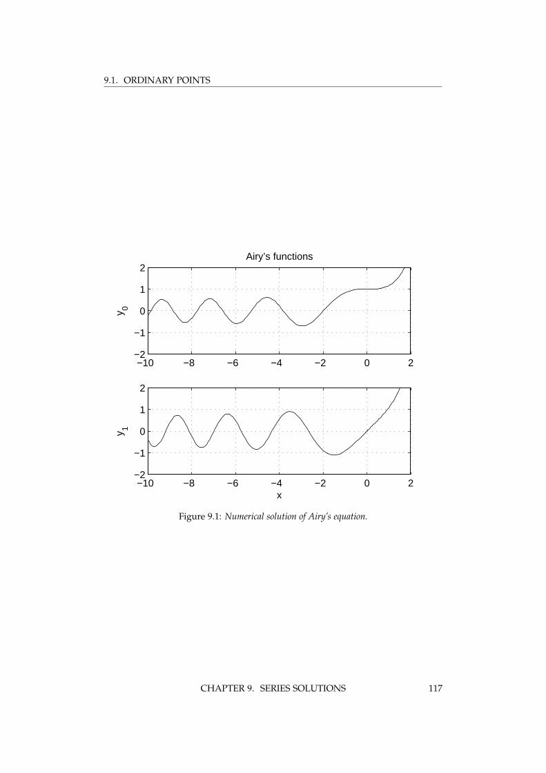
9.1. ORDINARY POINTS
−10 −8 −6 −4 −2 0 2−2
−1
0
1
2
y 0
Airy’s functions
−10 −8 −6 −4 −2 0 2−2
−1
0
1
2
x
y 1
Figure 9.1: Numerical solution of Airy’s equation.
CHAPTER 9. SERIES SOLUTIONS 117

9.1. ORDINARY POINTS
118 CHAPTER 9. SERIES SOLUTIONS
Chapter 10
Systems of linear differentialequations
Reference: Boyce and DiPrima, Chapter 7
Here, we consider the simplest case of a system of two coupled homogeneous linearfirst-order equations with constant coefficients. The general system is given by
x1 = ax1 + bx2, x2 = cx1 + dx2, (10.1)
or in matrix form asddt
(x1x2
)=
(a bc d
)(x1x2
).
The short-hand notation will bex = Ax. (10.2)
Although we can write these two first-order equations as a single second-orderequation, we will instead make use of our newly learned techniques in matrix al-gebra. We will also introduce the important concept of the phase space, and thephysical problem of coupled oscillators.
10.1 Distinct real eigenvalues
We illustrate the solution method by example.
Example: Find the general solution of x1 = x1 + x2, x2 = 4x1 + x2.
View tutorial on YouTube
The equation to be solved may be rewritten in matrix form as
ddt
(x1x2
)=
(1 14 1
)(x1x2
), (10.3)
or in short hand as (10.2).We take as our ansatz x(t) = veλt, where v and λ are independent of t. Upon
substitution into (10.2), we obtain
λveλt = Aveλt;
and upon cancellation of the exponential, we obtain the eigenvalue problem
Av = λv. (10.4)
Finding the characteristic equation using (5.4), we have
0 = det (A− λI)
= λ2 − 2λ− 3= (λ− 3)(λ + 1).
119
10.1. DISTINCT REAL EIGENVALUES
Therefore, the two eigenvalues are λ1 = 3 and λ2 = −1.To determine the corresponding eigenvectors, we substitute the eigenvalues suc-
cessively into(A− λI)v = 0. (10.5)
We will write the corresponding eigenvectors v1 and v2 using the matrix notation(v1 v2
)=
(v11 v12v21 v22
),
where the components of v1 and v2 are written with subscripts corresponding tothe first and second columns of a 2-by-2 matrix.
For λ1 = 3, and unknown eigenvector v1, we have from (10.5)
−2v11 + v21 = 0,4v11 − 2v21 = 0.
Clearly, the second equation is just the first equation multiplied by −2, so only oneequation is linearly independent. This will always be true, so for the 2-by-2 casewe need only consider the first row of the matrix. The first eigenvector thereforesatisfies v21 = 2v11. Recall that an eigenvector is only unique up to multiplicationby a constant: we may therefore take v11 = 1 for convenience.
For λ2 = −1, and eigenvector v2 = (v12, v22)T , we have from (10.5)
2v12 + v22 = 0,
so that v22 = −2v12. Here, we take v12 = 1.Therefore, our eigenvalues and eigenvectors are given by
λ1 = 3, v1 =
(12
); λ2 = −1, v2 =
(1−2
).
Using the principle of superposition, the general solution to the ode is therefore
X(t) = c1v1eλ1t + c2v2eλ2t,
or explicitly writing out the components,
x1(t) = c1e3t + c2e−t,
x2(t) = 2c1e3t − 2c2e−t. (10.6)
We can obtain a new perspective on the solution by drawing a phase portrait,shown in Fig. 10.1, with “x-axis” x1 and “y-axis” x2. Each curve corresponds to adifferent initial condition, and represents the trajectory of a particle with velocitygiven by the differential equation. The dark lines represent trajectories along thedirection of the eigenvectors. If c2 = 0, the motion is along the eigenvector v1with x2 = 2x1 and the motion with increasing time is away from the origin (arrowspointing out) since the eigenvalue λ1 = 3 > 0. If c1 = 0, the motion is along theeigenvector v2 with x2 = −2x1 and motion is towards the origin (arrows pointingin) since the eigenvalue λ2 = −1 < 0. When the eigenvalues are real and of oppositesigns, the origin is called a saddle point. Almost all trajectories (with the exceptionof those with initial conditions exactly satisfying x2(0) = −2x1(0)) eventually moveaway from the origin as t increases. When the eigenvalues are real and of the samesign, the origin is called a node. A node can be stable (negative eigenvalues) orunstable (positive eigenvalues).
120 CHAPTER 10. SYSTEMS OF LINEAR DIFFERENTIAL EQUATIONS

10.2. SOLUTION BY DIAGONALIZATION
-2 -1 0 1 2
x1
-2
-1
0
1
2
x 2
Figure 10.1: Phase portrait for example with two real eigenvalues of opposite sign.
10.2 Solution by diagonalization
Another way to view the problem of coupled first-order linear odes is from theperspective of matrix diagonalization. With
x = Ax, (10.7)
we suppose A can be diagonalized using
S−1AS = Λ, (10.8)
where Λ is the diagonal eigenvalue matrix, and S holds the eigenvectors. We canchange variables in (10.7) using
x = Sy (10.9)
and obtainSy = ASy.
Multiplication on the left by S−1 and using (10.8) results in
y = S−1ASy= Λy.
The first-order differential equations in the y-variables are now uncoupled and canbe immediately solved, and the x-variables can be recovered using (10.9).Example: Solve the previous example
ddt
(x1x2
)=
(1 14 1
)(x1x2
),
by the diagonalization method.
CHAPTER 10. SYSTEMS OF LINEAR DIFFERENTIAL EQUATIONS 121
10.3. SOLUTION BY THE MATRIX EXPONENTIAL
The eigenvalues and eigenvectors are known, and we have
Λ =
(3 00 −1
), S =
(1 12 −2
),
and the uncoupled y-equations are given by
y1 = 3y1, y2 = −y2,
with solution
y1(t) = c1e3t, y2 = c2e−t.
Transforming back to the x-variables using (10.9), we have(x1x2
)=
(1 12 −2
)(c1e3t
c2e−t
)=
(c1e3t + c2e−t
2c1e3t − 2c2e−t
),
which agrees with solution (10.6).
10.3 Solution by the matrix exponential
Another interesting approach to this problem makes use of the matrix exponential.Let A be a square matrix, tA the matrix A multiplied by the scalar t, and An thematrix A multiplied by itself n times. We define the matrix exponential function etA
similar to the way the exponential function may be defined using its Taylor series.The corresponding definition is
etA = I + tA +t2A2
2!+
t3A3
3!+
t4A4
4!+ . . . .
We can differentiate etA with respect to t and obtain
ddt
etA = A + tA2 +t2A3
2!+
t3A4
3!+ . . .
= A(
I + tA +t2A2
2!+
t3A3
3!+ . . .
)= AetA,
as one would expect from differentiating the exponential function. We can thereforeformally write the solution of
x = Ax
as
x(t) = etAx(0).
122 CHAPTER 10. SYSTEMS OF LINEAR DIFFERENTIAL EQUATIONS
10.4. DISTINCT COMPLEX-CONJUGATE EIGENVALUES
If the matrix A is diagonalizable such that A = SΛS−1, then observe that
etA = etSΛS−1
= I + tSΛS−1 +t2(SΛS−1)2
2!+
t3(SΛS−1)3
3!+ . . .
= I + tSΛS−1 +t2SΛ2S−1
2!+
t3SΛ3S−1
3!+ . . .
= S(
I + tΛ +t2Λ2
2!+
t3Λ3
3!+ . . .
)S−1
= SetΛS−1.
If Λ is a diagonal matrix with diagonal elements λ1, λ2, etc., then the matrix ex-ponential etΛ is also a diagonal matrix with diagonal elements given by eλ1t, eλ2t,etc. We can now use the matrix exponential to solve a system of linear differentialequations.Example: Solve the previous example
ddt
(x1x2
)=
(1 14 1
)(x1x2
),
by matrix exponentiation.We know that
Λ =
(3 00 −1
), S =
(1 12 −2
), S−1 = −1
4
(−2 −1−2 1
).
The solution to the system of differential equations is then given by
x(t) = etAx(0)
= SetΛS−1x(0)
= −14
(1 12 −2
)(e3t 00 e−t
)(−2 −1−2 1
)x(0).
Successive matrix multiplication results in
x1(t) =14(2x1(0) + x2(0))e3t +
14(2x1(0)− x2(0))e−t,
x2(t) =12(2x1(0) + x2(0))e3t − 1
2(2x1(0)− x2(0))e−t,
which is the same solution as previously found, but here the c1 and c2 free coeffi-cients are replaced by the initial values of x(0).
10.4 Distinct complex-conjugate eigenvalues
Example: Find the general solution of x1 = − 12 x1 + x2, x2 = −x1 − 1
2 x2.
View tutorial on YouTube
The equations in matrix form are
ddt
(x1x2
)=
(−1/2 1−1 −1/2
)(x1x2
).
CHAPTER 10. SYSTEMS OF LINEAR DIFFERENTIAL EQUATIONS 123
10.4. DISTINCT COMPLEX-CONJUGATE EIGENVALUES
The ansatz x = veλt leads to the equation
0 = det (A− λI)
= λ2 + λ +54
.
Therefore, λ = −1/2± i; and we observe that the eigenvalues occur as a complexconjugate pair. We will denote the two eigenvalues as
λ = −12+ i and λ = −1
2− i.
Now, if A a real matrix, then Av = λv implies Av = λv, so the eigenvectors alsooccur as a complex conjugate pair. The eigenvector v associated with eigenvalue λsatisfies −iv1 + v2 = 0, and normalizing with v1 = 1, we have
v =
(1i
).
We have therefore determined two independent complex solutions to the ode, thatis,
veλt and veλt,
and we can form a linear combination of these two complex solutions to constructtwo independent real solutions. Namely, if the complex functions z(t) and z(t) arewritten as
z(t) = Re{z(t)}+ iIm{z(t)}, z(t) = Re{z(t)} − iIm{z(t)},
then two real functions can be constructed from the following linear combinationsof z and z:
z + z2
= Re{z(t)} andz− z
2i= Im{z(t)}.
Thus the two real vector functions that can be constructed from our two complexvector functions are
Re{veλt} = Re{(
1i
)e(−
12+i)t
}= e−
12 tRe
{(1i
)(cos t + i sin t)
}= e−
12 t(
cos t− sin t
);
and
Im{veλt} = e−12 tIm
{(1i
)(cos t + i sin t)
}= e−
12 t(
sin tcos t
).
Taking a linear superposition of these two real solutions yields the general solutionto the ode, given by
x = e−12 t[
A(
cos t− sin t
)+ B
(sin tcos t
)].
124 CHAPTER 10. SYSTEMS OF LINEAR DIFFERENTIAL EQUATIONS
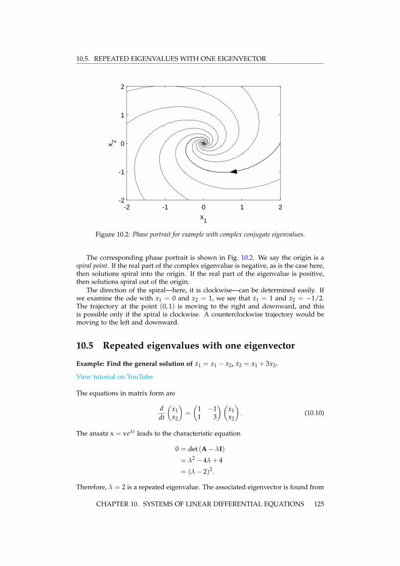
10.5. REPEATED EIGENVALUES WITH ONE EIGENVECTOR
-2 -1 0 1 2
x1
-2
-1
0
1
2
x 2
Figure 10.2: Phase portrait for example with complex conjugate eigenvalues.
The corresponding phase portrait is shown in Fig. 10.2. We say the origin is aspiral point. If the real part of the complex eigenvalue is negative, as is the case here,then solutions spiral into the origin. If the real part of the eigenvalue is positive,then solutions spiral out of the origin.
The direction of the spiral—here, it is clockwise—can be determined easily. Ifwe examine the ode with x1 = 0 and x2 = 1, we see that x1 = 1 and x2 = −1/2.The trajectory at the point (0, 1) is moving to the right and downward, and thisis possible only if the spiral is clockwise. A counterclockwise trajectory would bemoving to the left and downward.
10.5 Repeated eigenvalues with one eigenvector
Example: Find the general solution of x1 = x1 − x2, x2 = x1 + 3x2.
View tutorial on YouTube
The equations in matrix form are
ddt
(x1x2
)=
(1 −11 3
)(x1x2
). (10.10)
The ansatz x = veλt leads to the characteristic equation
0 = det (A− λI)
= λ2 − 4λ + 4
= (λ− 2)2.
Therefore, λ = 2 is a repeated eigenvalue. The associated eigenvector is found from
CHAPTER 10. SYSTEMS OF LINEAR DIFFERENTIAL EQUATIONS 125
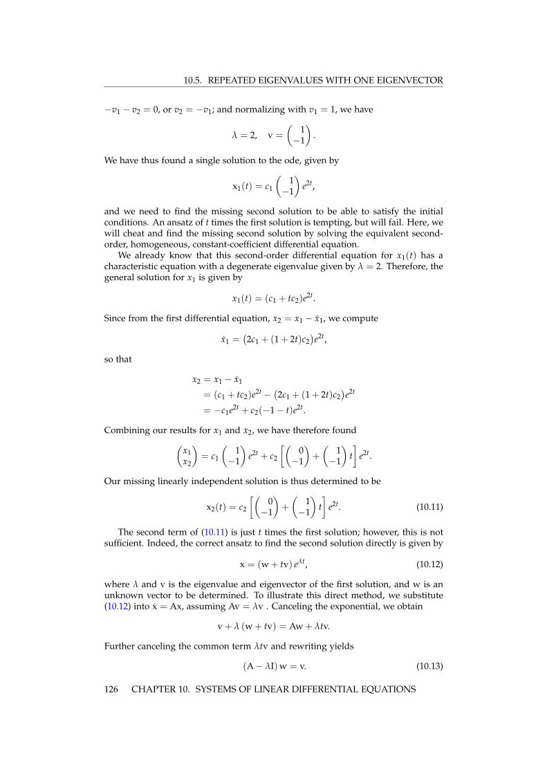
10.5. REPEATED EIGENVALUES WITH ONE EIGENVECTOR
−v1 − v2 = 0, or v2 = −v1; and normalizing with v1 = 1, we have
λ = 2, v =
(1−1
).
We have thus found a single solution to the ode, given by
x1(t) = c1
(1−1
)e2t,
and we need to find the missing second solution to be able to satisfy the initialconditions. An ansatz of t times the first solution is tempting, but will fail. Here, wewill cheat and find the missing second solution by solving the equivalent second-order, homogeneous, constant-coefficient differential equation.
We already know that this second-order differential equation for x1(t) has acharacteristic equation with a degenerate eigenvalue given by λ = 2. Therefore, thegeneral solution for x1 is given by
x1(t) = (c1 + tc2)e2t.
Since from the first differential equation, x2 = x1 − x1, we compute
x1 =(2c1 + (1 + 2t)c2
)e2t,
so that
x2 = x1 − x1
= (c1 + tc2)e2t −(2c1 + (1 + 2t)c2
)e2t
= −c1e2t + c2(−1− t)e2t.
Combining our results for x1 and x2, we have therefore found(x1x2
)= c1
(1−1
)e2t + c2
[(0−1
)+
(1−1
)t]
e2t.
Our missing linearly independent solution is thus determined to be
x2(t) = c2
[(0−1
)+
(1−1
)t]
e2t. (10.11)
The second term of (10.11) is just t times the first solution; however, this is notsufficient. Indeed, the correct ansatz to find the second solution directly is given by
x = (w + tv) eλt, (10.12)
where λ and v is the eigenvalue and eigenvector of the first solution, and w is anunknown vector to be determined. To illustrate this direct method, we substitute(10.12) into x = Ax, assuming Av = λv . Canceling the exponential, we obtain
v + λ (w + tv) = Aw + λtv.
Further canceling the common term λtv and rewriting yields
(A− λI)w = v. (10.13)
126 CHAPTER 10. SYSTEMS OF LINEAR DIFFERENTIAL EQUATIONS

10.6. NORMAL MODES
-2 -1 0 1 2
x1
-2
-1
0
1
2
x 2
Figure 10.3: Phase portrait for example with only one eigenvector.
If A has only a single linearly independent eigenvector v, then (10.13) can be solvedfor w (otherwise, it cannot). Using A, λ and v of our present example, (10.13) is thesystem of equations given by(
−1 −11 1
)(w1w2
)=
(1−1
).
The first and second equation are the same, so that w2 = −(w1 + 1). Therefore,
w =
(w1
−(w1 + 1)
)= w1
(1−1
)+
(0−1
).
Notice that the first term repeats the first found solution, i.e., a constant times theeigenvector, and the second term is new. We therefore take w1 = 0 and obtain
w =
(0−1
),
as before.The phase portrait for this ode is shown in Fig. 10.3. The dark line is the single
eigenvector v of the matrix A. When there is only a single eigenvector, the origin iscalled an improper node.
10.6 Normal modes
View tutorials on YouTube: Part 1 Part 2
CHAPTER 10. SYSTEMS OF LINEAR DIFFERENTIAL EQUATIONS 127
10.6. NORMAL MODES
m m
k kK
x1 x2Figure 10.4: Top view of a double mass, triple spring system.
We now consider an application of the eigenvector analysis to the coupled mass-spring system shown in Fig. 10.4. The position variables x1 and x2 are measuredfrom the equilibrium positions of the masses. Hooke’s law states that the springforce is linearly proportional to the extension length of the spring, measured fromequilibrium. By considering the extension of the spring and the sign of the force,we write Newton’s law F = ma separately for each mass:
mx1 = −kx1 − K(x1 − x2),mx2 = −kx2 − K(x2 − x1).
Further rewriting by collecting terms proportional to x1 and x2 yields
mx1 = −(k + K)x1 + Kx2,mx2 = Kx1 − (k + K)x2.
The equations for the coupled mass-spring system form a system of two second-order linear homogeneous odes. In matrix form, mx = Ax, or explicitly,
md2
dt2
(x1x2
)=
(−(k + K) K
K −(k + K)
)(x1x2
). (10.14)
In analogy to a system of first-order equations, we try the ansatz x = vert, and uponsubstitution into (10.14) we obtain the eigenvalue problem Av = λv, with λ = mr2.The eigenvalues are determined by solving the characteristic equation
0 = det (A− λI)
=
∣∣∣∣−(k + K)− λ KK −(k + K)− λ
∣∣∣∣= (λ + k + K)2 − K2.
The solution for λ isλ = −k− K± K,
and the two eigenvalues are
λ1 = −k, λ2 = −(k + 2K).
The corresponding values of r in our ansatz x = vert, with r = ±√
λ/m, are
r1 = i√
k/m, r1, r2 = i√(k + 2K)/m, r2.
128 CHAPTER 10. SYSTEMS OF LINEAR DIFFERENTIAL EQUATIONS
10.6. NORMAL MODES
Since the values of r are pure imaginary, we know that x1(t) and x2(t) will oscillatewith angular frequencies ω1 = Im{r1} and ω2 = Im{r2}, that is,
ω1 =√
k/m, ω2 =√(k + 2K)/m.
The positions of the oscillating masses in general contain time dependencies of theform sin ω1t, cos ω1t, and sin ω2t, cos ω2t.
It is of further interest to determine the eigenvectors, or so-called normal modesof oscillation, associated with the two distinct angular frequencies. With specificinitial conditions proportional to an eigenvector, the mass will oscillate with a singlefrequency. The eigenvector with eigenvalue λ1 satisfies
−Kv11 + Kv12 = 0,
so that v11 = v12. The normal mode with frequency ω1 =√
k/m thus follows amotion where x1 = x2. Referring to Fig. 10.4, during this motion the center springlength does not change, which is why the frequency of oscillation is independentof K.
Next, we determine the eigenvector with eigenvalue λ2:
Kv21 + Kv22 = 0,
so that v21 = −v22. The normal mode with frequency ω2 =√(k + 2K)/m thus
follows a motion where x1 = −x2. Again referring to Fig. 10.4, during this motionthe two equal masses symmetrically push or pull against each side of the middlespring.
A general solution for x(t) can be constructed from the eigenvalues and eigen-vectors. Our ansatz was X = Vert, and for each of two eigenvectors V, we have apair of complex conjugate values for r. Accordingly, we first apply the principle ofsuperposition to obtain four real solutions, and then apply the principle again toobtain the general solution. With ω1 =
√k/m and ω2 =
√(k + 2K)/m, the general
solution is given by(x1x2
)=
(11
)(A cos ω1t + B sin ω1t) +
(1−1
)(C cos ω2t + D sin ω2t) ,
where the now real constants A, B, C, and D can be determined from the fourindependent initial conditions, x1(0), x2(0), x1(0), and x2(0).
CHAPTER 10. SYSTEMS OF LINEAR DIFFERENTIAL EQUATIONS 129

10.6. NORMAL MODES
130 CHAPTER 10. SYSTEMS OF LINEAR DIFFERENTIAL EQUATIONS
Chapter 11
Nonlinear differentialequations
Reference: Strogatz, Sections 2.2, 2.4, 3.1, 3.2, 3.4, 6.3, 6.4, 8.2
We now turn our attention to nonlinear differential equations. In particular, westudy how small changes in the parameters of a system can result in qualitativechanges in the dynamics. These qualitative changes in the dynamics are calledbifurcations. To understand bifurcations, we first need to understand the conceptsof fixed points and stability.
11.1 Fixed points and stability
11.1.1 One dimensionView tutorial on YouTube
Consider the one-dimensional differential equation for x = x(t) given by
x = f (x). (11.1)
We say that x∗ is a fixed point, or equilibrium point, of (11.1) if f (x∗) = 0. At the fixedpoint, x = 0. The terminology fixed point is used since the solution to (11.1) withinitial condition x(0) = x∗ is x(t) = x∗ for all time t.
A fixed point, however, can be stable or unstable. A fixed point is said to bestable if a small perturbation of the solution from the fixed point decays in time; it issaid to be unstable if a small perturbation grows in time. We can determine stabilityby a linear analysis. Let x = x∗ + ε(t), where ε represents a small perturbation ofthe solution from the fixed point x∗. Because x∗ is a constant, x = ε; and becausex∗ is a fixed point, f (x∗) = 0. Taylor series expanding about ε = 0, we have
ε = f (x∗ + ε)
= f (x∗) + ε f ′(x∗) + . . .
= ε f ′(x∗) + . . . .
The omitted terms in the Taylor series expansion are proportional to ε2, and can bemade negligible over a short time interval with respect to the kept term, propor-tional to ε, by taking ε(0) sufficiently small. Therefore, at least over short times,the differential equation to be considered, ε = f ′(x∗)ε, is linear and has by now thefamiliar solution
ε(t) = ε(0)e f ′(x∗)t.
The perturbation of the fixed point solution x(t) = x∗ thus decays exponentiallyif f ′(x∗) < 0, and we say the fixed point is stable. If f ′(x∗) > 0, the perturbationgrows exponentially and we say the fixed point is unstable. If f ′(x∗) = 0, we saythe fixed point is marginally stable, and the next higher-order term in the Taylorseries expansion must be considered.
131
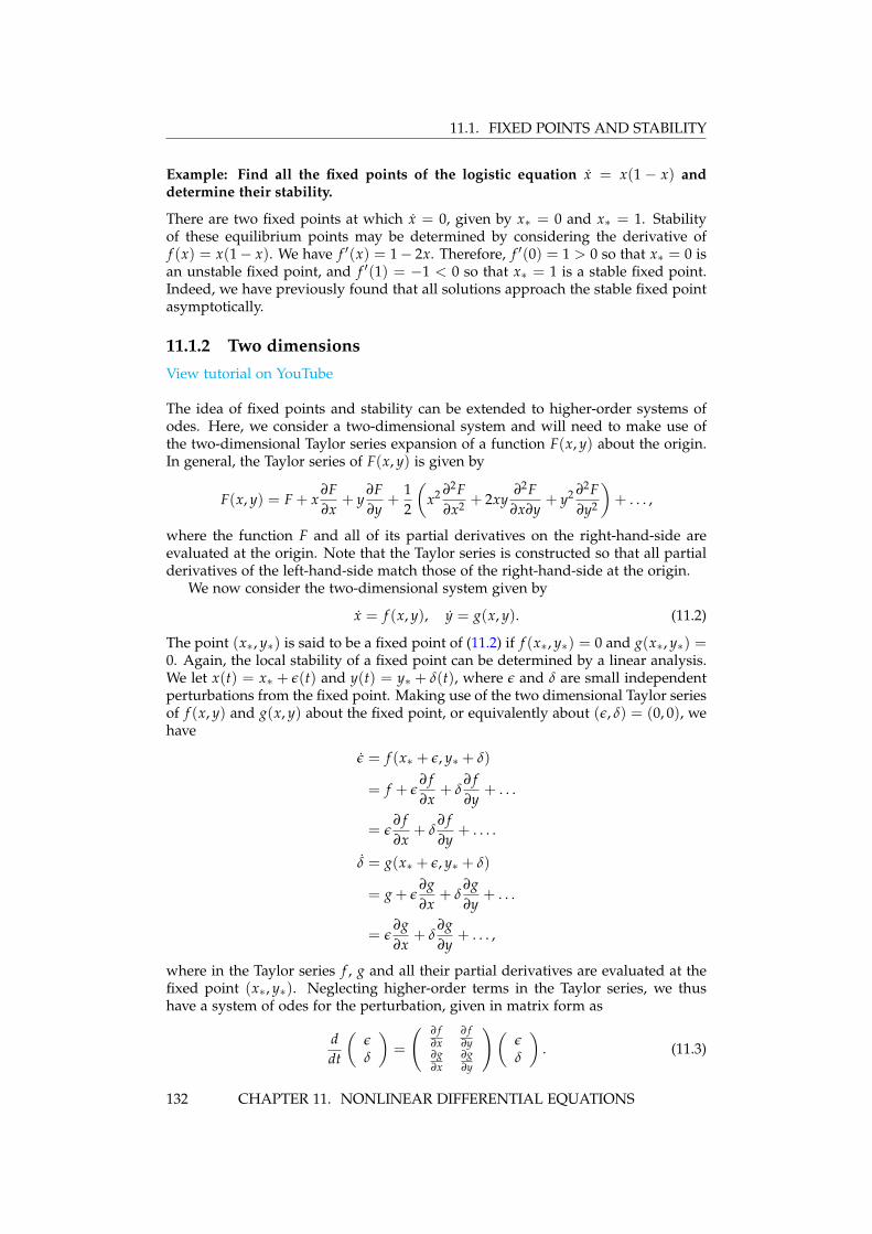
11.1. FIXED POINTS AND STABILITY
Example: Find all the fixed points of the logistic equation x = x(1 − x) anddetermine their stability.
There are two fixed points at which x = 0, given by x∗ = 0 and x∗ = 1. Stabilityof these equilibrium points may be determined by considering the derivative off (x) = x(1− x). We have f ′(x) = 1− 2x. Therefore, f ′(0) = 1 > 0 so that x∗ = 0 isan unstable fixed point, and f ′(1) = −1 < 0 so that x∗ = 1 is a stable fixed point.Indeed, we have previously found that all solutions approach the stable fixed pointasymptotically.
11.1.2 Two dimensionsView tutorial on YouTube
The idea of fixed points and stability can be extended to higher-order systems ofodes. Here, we consider a two-dimensional system and will need to make use ofthe two-dimensional Taylor series expansion of a function F(x, y) about the origin.In general, the Taylor series of F(x, y) is given by
F(x, y) = F + x∂F∂x
+ y∂F∂y
+12
(x2 ∂2F
∂x2 + 2xy∂2F
∂x∂y+ y2 ∂2F
∂y2
)+ . . . ,
where the function F and all of its partial derivatives on the right-hand-side areevaluated at the origin. Note that the Taylor series is constructed so that all partialderivatives of the left-hand-side match those of the right-hand-side at the origin.
We now consider the two-dimensional system given by
x = f (x, y), y = g(x, y). (11.2)
The point (x∗, y∗) is said to be a fixed point of (11.2) if f (x∗, y∗) = 0 and g(x∗, y∗) =0. Again, the local stability of a fixed point can be determined by a linear analysis.We let x(t) = x∗ + ε(t) and y(t) = y∗ + δ(t), where ε and δ are small independentperturbations from the fixed point. Making use of the two dimensional Taylor seriesof f (x, y) and g(x, y) about the fixed point, or equivalently about (ε, δ) = (0, 0), wehave
ε = f (x∗ + ε, y∗ + δ)
= f + ε∂ f∂x
+ δ∂ f∂y
+ . . .
= ε∂ f∂x
+ δ∂ f∂y
+ . . . .
δ = g(x∗ + ε, y∗ + δ)
= g + ε∂g∂x
+ δ∂g∂y
+ . . .
= ε∂g∂x
+ δ∂g∂y
+ . . . ,
where in the Taylor series f , g and all their partial derivatives are evaluated at thefixed point (x∗, y∗). Neglecting higher-order terms in the Taylor series, we thushave a system of odes for the perturbation, given in matrix form as
ddt
(εδ
)=
( ∂ f∂x
∂ f∂y
∂g∂x
∂g∂y
)(εδ
). (11.3)
132 CHAPTER 11. NONLINEAR DIFFERENTIAL EQUATIONS
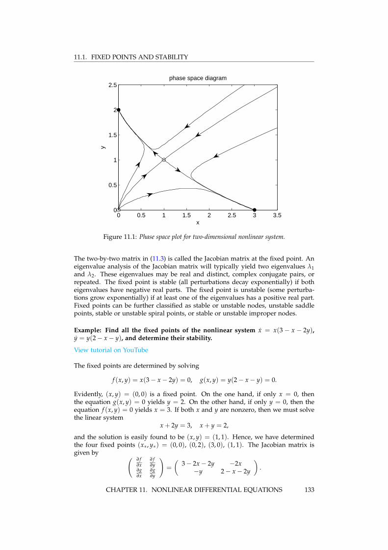
11.1. FIXED POINTS AND STABILITY
0 0.5 1 1.5 2 2.5 3 3.50
0.5
1
1.5
2
2.5
x
y
phase space diagram
Figure 11.1: Phase space plot for two-dimensional nonlinear system.
The two-by-two matrix in (11.3) is called the Jacobian matrix at the fixed point. Aneigenvalue analysis of the Jacobian matrix will typically yield two eigenvalues λ1and λ2. These eigenvalues may be real and distinct, complex conjugate pairs, orrepeated. The fixed point is stable (all perturbations decay exponentially) if botheigenvalues have negative real parts. The fixed point is unstable (some perturba-tions grow exponentially) if at least one of the eigenvalues has a positive real part.Fixed points can be further classified as stable or unstable nodes, unstable saddlepoints, stable or unstable spiral points, or stable or unstable improper nodes.
Example: Find all the fixed points of the nonlinear system x = x(3 − x − 2y),y = y(2− x− y), and determine their stability.
View tutorial on YouTube
The fixed points are determined by solving
f (x, y) = x(3− x− 2y) = 0, g(x, y) = y(2− x− y) = 0.
Evidently, (x, y) = (0, 0) is a fixed point. On the one hand, if only x = 0, thenthe equation g(x, y) = 0 yields y = 2. On the other hand, if only y = 0, then theequation f (x, y) = 0 yields x = 3. If both x and y are nonzero, then we must solvethe linear system
x + 2y = 3, x + y = 2,
and the solution is easily found to be (x, y) = (1, 1). Hence, we have determinedthe four fixed points (x∗, y∗) = (0, 0), (0, 2), (3, 0), (1, 1). The Jacobian matrix isgiven by ( ∂ f
∂x∂ f∂y
∂g∂x
∂g∂y
)=
(3− 2x− 2y −2x−y 2− x− 2y
).
CHAPTER 11. NONLINEAR DIFFERENTIAL EQUATIONS 133
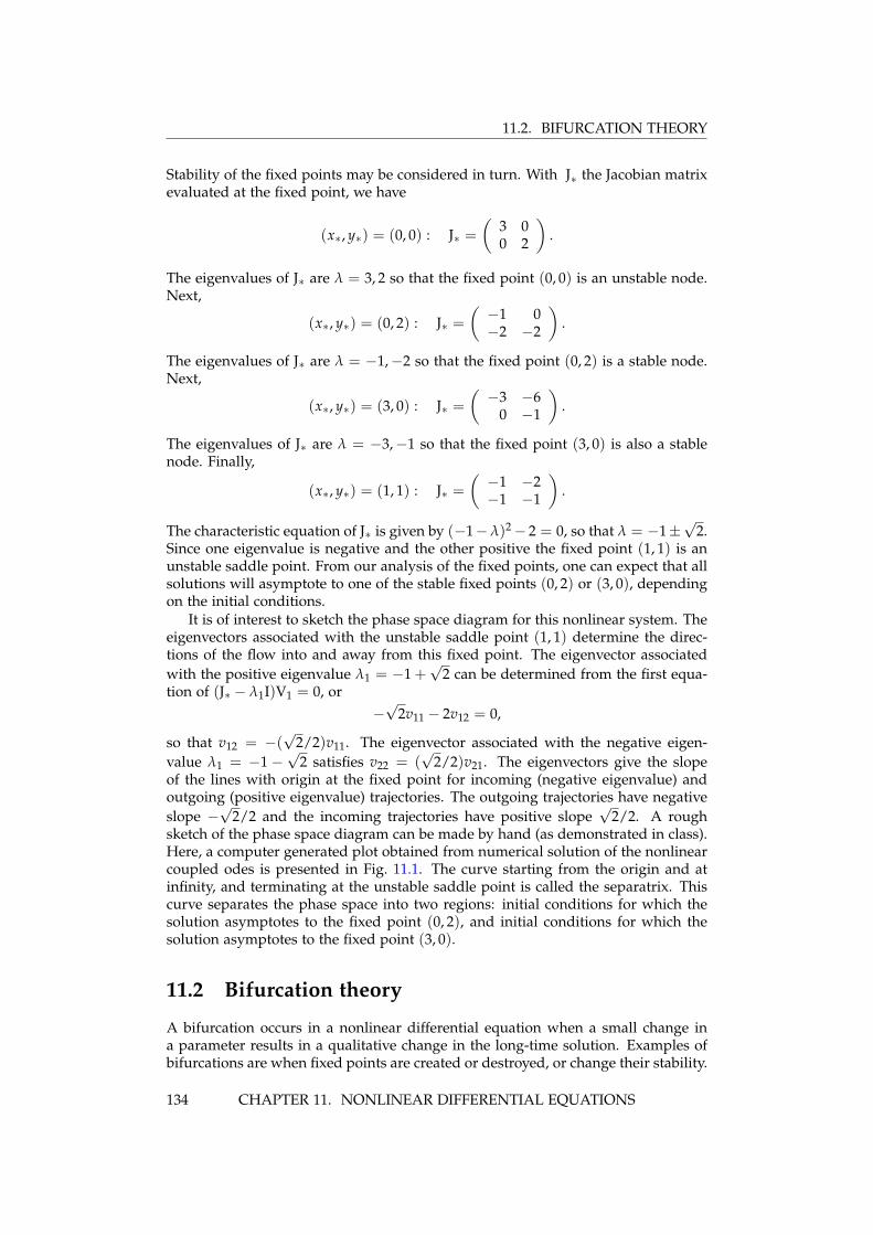
11.2. BIFURCATION THEORY
Stability of the fixed points may be considered in turn. With J∗ the Jacobian matrixevaluated at the fixed point, we have
(x∗, y∗) = (0, 0) : J∗ =(
3 00 2
).
The eigenvalues of J∗ are λ = 3, 2 so that the fixed point (0, 0) is an unstable node.Next,
(x∗, y∗) = (0, 2) : J∗ =(−1 0−2 −2
).
The eigenvalues of J∗ are λ = −1,−2 so that the fixed point (0, 2) is a stable node.Next,
(x∗, y∗) = (3, 0) : J∗ =(−3 −6
0 −1
).
The eigenvalues of J∗ are λ = −3,−1 so that the fixed point (3, 0) is also a stablenode. Finally,
(x∗, y∗) = (1, 1) : J∗ =(−1 −2−1 −1
).
The characteristic equation of J∗ is given by (−1−λ)2− 2 = 0, so that λ = −1±√
2.Since one eigenvalue is negative and the other positive the fixed point (1, 1) is anunstable saddle point. From our analysis of the fixed points, one can expect that allsolutions will asymptote to one of the stable fixed points (0, 2) or (3, 0), dependingon the initial conditions.
It is of interest to sketch the phase space diagram for this nonlinear system. Theeigenvectors associated with the unstable saddle point (1, 1) determine the direc-tions of the flow into and away from this fixed point. The eigenvector associatedwith the positive eigenvalue λ1 = −1 +
√2 can be determined from the first equa-
tion of (J∗ − λ1I)V1 = 0, or−√
2v11 − 2v12 = 0,
so that v12 = −(√
2/2)v11. The eigenvector associated with the negative eigen-value λ1 = −1−
√2 satisfies v22 = (
√2/2)v21. The eigenvectors give the slope
of the lines with origin at the fixed point for incoming (negative eigenvalue) andoutgoing (positive eigenvalue) trajectories. The outgoing trajectories have negativeslope −
√2/2 and the incoming trajectories have positive slope
√2/2. A rough
sketch of the phase space diagram can be made by hand (as demonstrated in class).Here, a computer generated plot obtained from numerical solution of the nonlinearcoupled odes is presented in Fig. 11.1. The curve starting from the origin and atinfinity, and terminating at the unstable saddle point is called the separatrix. Thiscurve separates the phase space into two regions: initial conditions for which thesolution asymptotes to the fixed point (0, 2), and initial conditions for which thesolution asymptotes to the fixed point (3, 0).
11.2 Bifurcation theory
A bifurcation occurs in a nonlinear differential equation when a small change ina parameter results in a qualitative change in the long-time solution. Examples ofbifurcations are when fixed points are created or destroyed, or change their stability.
134 CHAPTER 11. NONLINEAR DIFFERENTIAL EQUATIONS
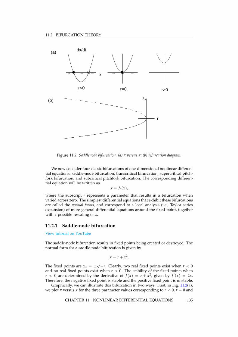
11.2. BIFURCATION THEORY
→ ← →
r<0
→ →
r=0 r>0
dx/dt
x
(a)
(b)x
*
r
Figure 11.2: Saddlenode bifurcation. (a) x versus x; (b) bifurcation diagram.
We now consider four classic bifurcations of one-dimensional nonlinear differen-tial equations: saddle-node bifurcation, transcritical bifurcation, supercritical pitch-fork bifurcation, and subcritical pitchfork bifurcation. The corresponding differen-tial equation will be written as
x = fr(x),
where the subscript r represents a parameter that results in a bifurcation whenvaried across zero. The simplest differential equations that exhibit these bifurcationsare called the normal forms, and correspond to a local analysis (i.e., Taylor seriesexpansion) of more general differential equations around the fixed point, togetherwith a possible rescaling of x.
11.2.1 Saddle-node bifurcation
View tutorial on YouTube
The saddle-node bifurcation results in fixed points being created or destroyed. Thenormal form for a saddle-node bifurcation is given by
x = r + x2.
The fixed points are x∗ = ±√−r. Clearly, two real fixed points exist when r < 0
and no real fixed points exist when r > 0. The stability of the fixed points whenr < 0 are determined by the derivative of f (x) = r + x2, given by f ′(x) = 2x.Therefore, the negative fixed point is stable and the positive fixed point is unstable.
Graphically, we can illustrate this bifurcation in two ways. First, in Fig. 11.2(a),we plot x versus x for the three parameter values corresponding to r < 0, r = 0 and
CHAPTER 11. NONLINEAR DIFFERENTIAL EQUATIONS 135
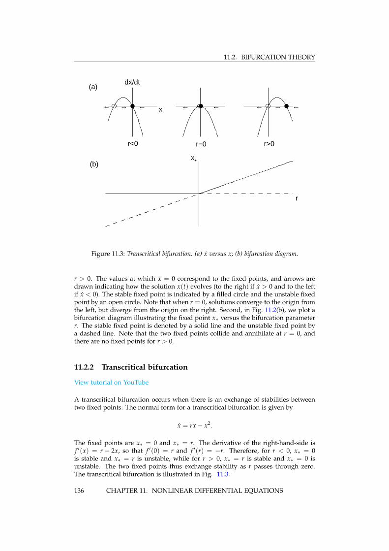
11.2. BIFURCATION THEORY
← → ←
r<0
dx/dt
x
(a)
← ←
r=0
←← →
r>0
x*
r
(b)
Figure 11.3: Transcritical bifurcation. (a) x versus x; (b) bifurcation diagram.
r > 0. The values at which x = 0 correspond to the fixed points, and arrows aredrawn indicating how the solution x(t) evolves (to the right if x > 0 and to the leftif x < 0). The stable fixed point is indicated by a filled circle and the unstable fixedpoint by an open circle. Note that when r = 0, solutions converge to the origin fromthe left, but diverge from the origin on the right. Second, in Fig. 11.2(b), we plot abifurcation diagram illustrating the fixed point x∗ versus the bifurcation parameterr. The stable fixed point is denoted by a solid line and the unstable fixed point bya dashed line. Note that the two fixed points collide and annihilate at r = 0, andthere are no fixed points for r > 0.
11.2.2 Transcritical bifurcation
View tutorial on YouTube
A transcritical bifurcation occurs when there is an exchange of stabilities betweentwo fixed points. The normal form for a transcritical bifurcation is given by
x = rx− x2.
The fixed points are x∗ = 0 and x∗ = r. The derivative of the right-hand-side isf ′(x) = r − 2x, so that f ′(0) = r and f ′(r) = −r. Therefore, for r < 0, x∗ = 0is stable and x∗ = r is unstable, while for r > 0, x∗ = r is stable and x∗ = 0 isunstable. The two fixed points thus exchange stability as r passes through zero.The transcritical bifurcation is illustrated in Fig. 11.3.
136 CHAPTER 11. NONLINEAR DIFFERENTIAL EQUATIONS

11.2. BIFURCATION THEORY
→ ←
r<0
dx/dt
x
(a)
→ ←
r=0
←→ ← →
r>0
x*
r
(b)
Figure 11.4: Supercritical pitchfork bifurcation. (a) x versus x; (b) bifurcation diagram.
11.2.3 Supercritical pitchfork bifurcation
View tutorial on YouTube
The pitchfork bifurcations occur in physical models where fixed points appear anddisappear in pairs due to some intrinsic symmetry of the problem. Pitchfork bi-furcations can come in one of two types. In the supercritical bifurcation, a pair ofstable fixed points are created at the bifurcation (or critical) point and exist after(super) the bifurcation. In the subcritical bifurcation, a pair of unstable fixed pointsare created at the bifurcation point and exist before (sub) the bifurcation.
The normal form for the supercritical pitchfork bifurcation is given by
x = rx− x3.
Note that the linear term results in exponential growth when r > 0 and the non-linear term stabilizes this growth. The fixed points are x∗ = 0 and x∗ = ±
√r, the
latter fixed points existing only when r > 0. The derivative of f is f ′(x) = r− 3x2
so that f ′(0) = r and f ′(±√
r) = −2r. Therefore, the fixed point x∗ = 0 is stable forr < 0 and unstable for r > 0 while the fixed points x = ±
√r exist and are stable for
r > 0. Notice that the fixed point x∗ = 0 becomes unstable as r crosses zero and twonew stable fixed points x∗ = ±
√r are born. The supercritical pitchfork bifurcation
is illustrated in Fig. 11.4.
11.2.4 Subcritical pitchfork bifurcation
View tutorial on YouTube
CHAPTER 11. NONLINEAR DIFFERENTIAL EQUATIONS 137

11.2. BIFURCATION THEORY
x*
r
Figure 11.5: Subcritical pitchfork bifurcation.
In the subcritical case, the cubic term is destabilizing. The normal form (to orderx3) is
x = rx + x3.
The fixed points are x∗ = 0 and x∗ = ±√−r, the latter fixed points existing only
when r ≤ 0. The derivative of the right-hand-side is f ′(x) = r+ 3x2 so that f ′(0) = rand f ′(±
√−r) = −2r. Therefore, the fixed point x∗ = 0 is stable for r < 0 and
unstable for r > 0 while the fixed points x = ±√−r exist and are unstable for
r < 0. There are no stable fixed points when r > 0.The absence of stable fixed points for r > 0 indicates that the neglect of terms of
higher-order in x than x3 in the normal form may be unwarranted. Keeping to theintrinsic symmetry of the equations (only odd powers of x) we can add a stabilizingnonlinear term proportional to x5. The extended normal form (to order x5) is
x = rx + x3 − x5,
and is somewhat more difficult to analyze. The fixed points are solutions of
x(r + x2 − x4) = 0.
The fixed point x∗ = 0 exists for all r, and four additional fixed points can be foundfrom the solutions of the quadratic equation in x2:
x∗ = ±√
12(1±
√1 + 4r).
These fixed points exist only if x∗ is real. Clearly, for the inner square-root to bereal, r ≥ −1/4. Also observe that 1−
√1 + 4r becomes negative for r > 0. We thus
have three intervals in r to consider, and these regions and their fixed points are
r < −14
: x∗ = 0 (one fixed point);
−14< r < 0 : x∗ = 0, x∗ = ±
√12(1±
√1 + 4r) (five fixed points);
r > 0 : x∗ = 0, x∗ = ±√
12(1 +
√1 + 4r) (three fixed points).
Stability is determined from f ′(x) = r + 3x2 − 5x4. Now, f ′(0) = r so x∗ = 0 isstable for r < 0 and unstable for r > 0. The calculation for the other four roots can
138 CHAPTER 11. NONLINEAR DIFFERENTIAL EQUATIONS
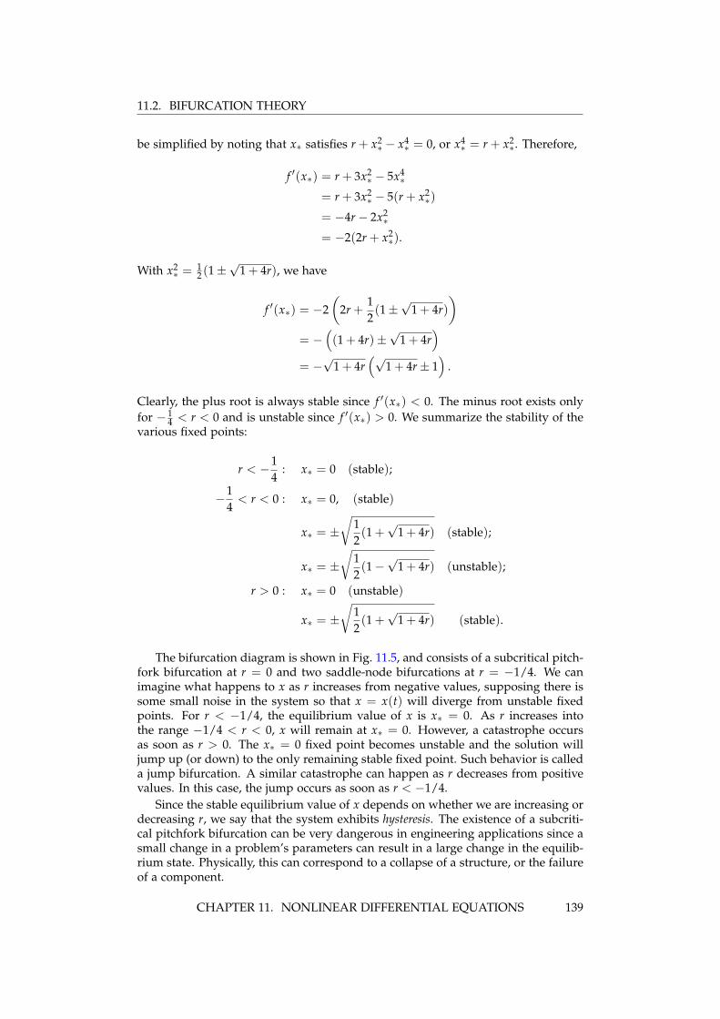
11.2. BIFURCATION THEORY
be simplified by noting that x∗ satisfies r + x2∗ − x4
∗ = 0, or x4∗ = r + x2
∗. Therefore,
f ′(x∗) = r + 3x2∗ − 5x4
∗
= r + 3x2∗ − 5(r + x2
∗)
= −4r− 2x2∗
= −2(2r + x2∗).
With x2∗ =
12 (1±
√1 + 4r), we have
f ′(x∗) = −2(
2r +12(1±
√1 + 4r)
)= −
((1 + 4r)±
√1 + 4r
)= −√
1 + 4r(√
1 + 4r± 1)
.
Clearly, the plus root is always stable since f ′(x∗) < 0. The minus root exists onlyfor − 1
4 < r < 0 and is unstable since f ′(x∗) > 0. We summarize the stability of thevarious fixed points:
r < −14
: x∗ = 0 (stable);
−14< r < 0 : x∗ = 0, (stable)
x∗ = ±√
12(1 +
√1 + 4r) (stable);
x∗ = ±√
12(1−
√1 + 4r) (unstable);
r > 0 : x∗ = 0 (unstable)
x∗ = ±√
12(1 +
√1 + 4r) (stable).
The bifurcation diagram is shown in Fig. 11.5, and consists of a subcritical pitch-fork bifurcation at r = 0 and two saddle-node bifurcations at r = −1/4. We canimagine what happens to x as r increases from negative values, supposing there issome small noise in the system so that x = x(t) will diverge from unstable fixedpoints. For r < −1/4, the equilibrium value of x is x∗ = 0. As r increases intothe range −1/4 < r < 0, x will remain at x∗ = 0. However, a catastrophe occursas soon as r > 0. The x∗ = 0 fixed point becomes unstable and the solution willjump up (or down) to the only remaining stable fixed point. Such behavior is calleda jump bifurcation. A similar catastrophe can happen as r decreases from positivevalues. In this case, the jump occurs as soon as r < −1/4.
Since the stable equilibrium value of x depends on whether we are increasing ordecreasing r, we say that the system exhibits hysteresis. The existence of a subcriti-cal pitchfork bifurcation can be very dangerous in engineering applications since asmall change in a problem’s parameters can result in a large change in the equilib-rium state. Physically, this can correspond to a collapse of a structure, or the failureof a component.
CHAPTER 11. NONLINEAR DIFFERENTIAL EQUATIONS 139
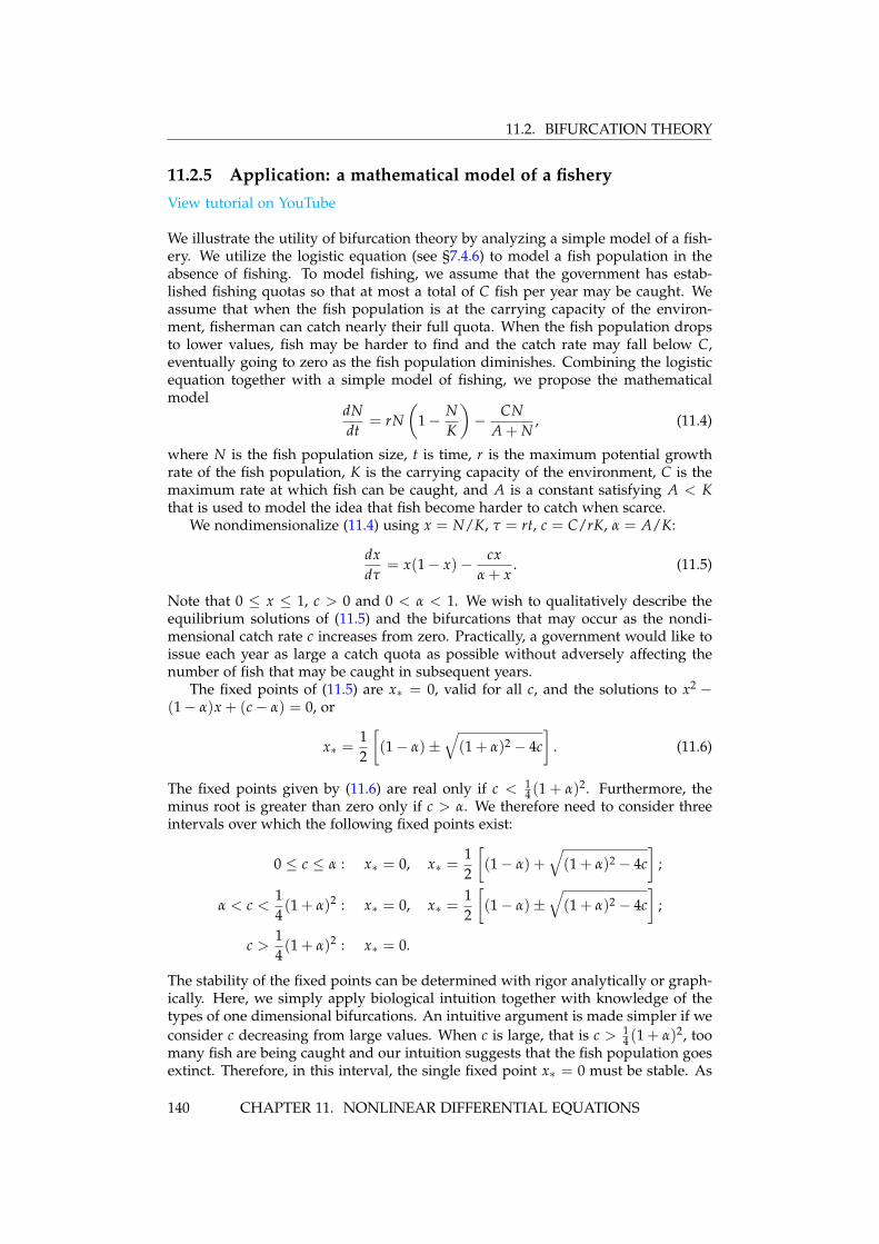
11.2. BIFURCATION THEORY
11.2.5 Application: a mathematical model of a fisheryView tutorial on YouTube
We illustrate the utility of bifurcation theory by analyzing a simple model of a fish-ery. We utilize the logistic equation (see §7.4.6) to model a fish population in theabsence of fishing. To model fishing, we assume that the government has estab-lished fishing quotas so that at most a total of C fish per year may be caught. Weassume that when the fish population is at the carrying capacity of the environ-ment, fisherman can catch nearly their full quota. When the fish population dropsto lower values, fish may be harder to find and the catch rate may fall below C,eventually going to zero as the fish population diminishes. Combining the logisticequation together with a simple model of fishing, we propose the mathematicalmodel
dNdt
= rN(
1− NK
)− CN
A + N, (11.4)
where N is the fish population size, t is time, r is the maximum potential growthrate of the fish population, K is the carrying capacity of the environment, C is themaximum rate at which fish can be caught, and A is a constant satisfying A < Kthat is used to model the idea that fish become harder to catch when scarce.
We nondimensionalize (11.4) using x = N/K, τ = rt, c = C/rK, α = A/K:
dxdτ
= x(1− x)− cxα + x
. (11.5)
Note that 0 ≤ x ≤ 1, c > 0 and 0 < α < 1. We wish to qualitatively describe theequilibrium solutions of (11.5) and the bifurcations that may occur as the nondi-mensional catch rate c increases from zero. Practically, a government would like toissue each year as large a catch quota as possible without adversely affecting thenumber of fish that may be caught in subsequent years.
The fixed points of (11.5) are x∗ = 0, valid for all c, and the solutions to x2 −(1− α)x + (c− α) = 0, or
x∗ =12
[(1− α)±
√(1 + α)2 − 4c
]. (11.6)
The fixed points given by (11.6) are real only if c < 14 (1 + α)2. Furthermore, the
minus root is greater than zero only if c > α. We therefore need to consider threeintervals over which the following fixed points exist:
0 ≤ c ≤ α : x∗ = 0, x∗ =12
[(1− α) +
√(1 + α)2 − 4c
];
α < c <14(1 + α)2 : x∗ = 0, x∗ =
12
[(1− α)±
√(1 + α)2 − 4c
];
c >14(1 + α)2 : x∗ = 0.
The stability of the fixed points can be determined with rigor analytically or graph-ically. Here, we simply apply biological intuition together with knowledge of thetypes of one dimensional bifurcations. An intuitive argument is made simpler if weconsider c decreasing from large values. When c is large, that is c > 1
4 (1 + α)2, toomany fish are being caught and our intuition suggests that the fish population goesextinct. Therefore, in this interval, the single fixed point x∗ = 0 must be stable. As
140 CHAPTER 11. NONLINEAR DIFFERENTIAL EQUATIONS
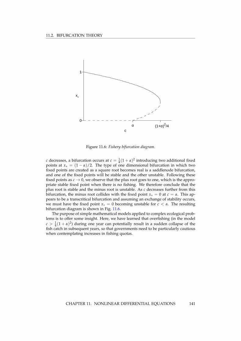
11.2. BIFURCATION THEORY
x*
c
1
0α (1+α)2/4
Figure 11.6: Fishery bifurcation diagram.
c decreases, a bifurcation occurs at c = 14 (1 + α)2 introducing two additional fixed
points at x∗ = (1− α)/2. The type of one dimensional bifurcation in which twofixed points are created as a square root becomes real is a saddlenode bifurcation,and one of the fixed points will be stable and the other unstable. Following thesefixed points as c→ 0, we observe that the plus root goes to one, which is the appro-priate stable fixed point when there is no fishing. We therefore conclude that theplus root is stable and the minus root is unstable. As c decreases further from thisbifurcation, the minus root collides with the fixed point x∗ = 0 at c = α. This ap-pears to be a transcritical bifurcation and assuming an exchange of stability occurs,we must have the fixed point x∗ = 0 becoming unstable for c < α. The resultingbifurcation diagram is shown in Fig. 11.6.
The purpose of simple mathematical models applied to complex ecological prob-lems is to offer some insight. Here, we have learned that overfishing (in the modelc > 1
4 (1 + α)2) during one year can potentially result in a sudden collapse of thefish catch in subsequent years, so that governments need to be particularly cautiouswhen contemplating increases in fishing quotas.
CHAPTER 11. NONLINEAR DIFFERENTIAL EQUATIONS 141


