Download - Ansys text book

FM-H6875.tex 28/11/2006 16: 7 page i

Engineering AnalysisWith ANSYS Software

This page intentionally left blank

FM-H6875.tex 28/11/2006 16: 7 page iii

Engineering AnalysisWith ANSYS Software

Y. Nakasone and S. YoshimotoDepartment of Mechanical EngineeringTokyo University of Science, Tokyo, Japan

T. A. StolarskiDepartment of Mechanical Engineering

School of Engineering and DesignBrunel University, Middlesex, UK

AMSTERDAM • BOSTON • HEIDELBERG • LONDON • NEW YORK • OXFORD

PARIS • SAN DIEGO • SAN FRANCISCO • SINGAPORE • SYDNEY • TOKYO

Butterworth-Heinemann is an imprint of Elsevier

FM-H6875.tex 28/11/2006 16: 7 page iv

Elsevier Butterworth-HeinemannLinacre House, Jordan Hill, Oxford OX2 8DP30 Corporate Drive, Burlington, MA 01803

First published 2006

Copyright © 2006 N. Nakasone, T. A. Stolarski and S. Yoshimoto. All rights reserved

The right of Howard D. Curtis to be identified as the author ofthis work has been asserted in accordance with the Copyright, Design andPatents Act 1988

No part of this publication may be reproduced in any material form (includingphotocopying or storing in any medium by electronic means and whether ornot transiently or incidentally to some other use of this publication) withoutthe written permission of the copyright holder except in accordance with theprovisions of the Copyright, Designs and Patents Act 1988 or under the terms of alicence issued by the Copyright Licensing Agency Ltd, 90 Tottenham Court Road,London, England W1T 4LP. Applications for the copyright holder’s writtenpermission to reproduce any part of this publication should be addressed tothe publisher

Permissions may be sought directly from Elsevier’s Science & TechnologyRights Department in Oxford, UK: phone (+44) 1865 843830,fax: (+44) 1865 853333, e-mail: [email protected] may also complete your request on-line via the Elsevier homepage(http://www.elsevier.com), by selecting ‘Customer Support’ and then‘Obtaining Permissions’

The copyrighted screen shots of the ANSYS software graphical interface thatappear throughout this book are used with permission of ANSYS, Inc.

ANSYS and any and all ANSYS, Inc. brand, product, service and feature names,logos and slogans are registered trademarks or trademarks of ANSYS, Inc. orits subsidiaries in the United States or other countries.

British Library Cataloguing in Publication DataA catalogue record for this book is available from the British Library

Library of Congress Cataloguing in Publication DataA catalogue record for this book is available from the Library of Congress

ISBN 0 7506 6875 X

For information on all Elsevier Butterworth-Heinemannpublications visit our website at http://books.elsevier.com

Typeset by Charon Tec Ltd (A Macmillan Company), Chennai, Indiawww.charontec.comPrinted and bound by MPG Books Ltd., Bodmin, Cornwall

FM-H6875.tex 28/11/2006 16: 7 page v

Contents

Preface xiii

The aims and scope of the book xv

Chapter

1 Basics of finite-element method 1

1.1 Method of weighted residuals 21.1.1 Sub-domain method (Finite volume method) 21.1.2 Galerkin method 4

1.2 Rayleigh–Ritz method 51.3 Finite-element method 7

1.3.1 One-element case 101.3.2 Three-element case 11

1.4 FEM in two-dimensional elastostatic problems 141.4.1 Elements of finite-element procedures in the analysis of

plane elastostatic problems 151.4.2 Fundamental formulae in plane elastostatic problems 16

1.4.2.1 Equations of equilibrium 161.4.2.2 Strain–displacement relations 161.4.2.3 Stress–strain relations (constitutive equations) 171.4.2.4 Boundary conditions 19

1.4.3 Variational formulae in elastostatic problems: the principleof virtual work 21

1.4.4 Formulation of the fundamental finite-element equationsin plane elastostatic problems 211.4.4.1 Strain–displacement matrix or [B] matrix 211.4.4.2 Stress–strain matrix or [D] matrix 251.4.4.3 Element stiffness equations 251.4.4.4 Global stiffness equations 271.4.4.5 Example: Finite-element calculations for a square

plate subjected to uniaxial uniform tension 30Bibliography 34

v

FM-H6875.tex 28/11/2006 16: 7 page vi

vi Contents

Chapter

2 Overview of ANSYS structure and visualcapabilities 37

2.1 Introduction 372.2 Starting the program 38

2.2.1 Preliminaries 382.2.2 Saving and restoring jobs 402.2.3 Organization of files 412.2.4 Printing and plotting 422.2.5 Exiting the program 43

2.3 Preprocessing stage 432.3.1 Building a model 43

2.3.1.1 Defining element types and real constants 442.3.1.2 Defining material properties 46

2.3.2 Construction of the model 472.3.2.1 Creating the model geometry 472.3.2.2 Applying loads 48

2.4 Solution stage 492.5 Postprocessing stage 50

Chapter

3 Application of ANSYS to stress analysis 51

3.1 Cantilever beam 513.1.1 Example problem: A cantilever beam 523.1.2 Problem description 53

3.1.2.1 Review of the solutions obtained by theelementary beam theory 53

3.1.3 Analytical procedures 533.1.3.1 Creation of an analytical model 533.1.3.2 Input of the elastic properties of the beam

material 563.1.3.3 Finite-element discretization of the beam area 573.1.3.4 Input of boundary conditions 623.1.3.5 Solution procedures 713.1.3.6 Graphical representation of the results 73

3.1.4 Comparison of FEM results with experimental ones 763.1.5 Problems to solve 76

Appendix: Procedures for creating stepped beams 80A3.1 Creation of a stepped beam 80

A3.1.1 How to cancel the selection of areas 81A3.2 Creation of a stepped beam with a rounded fillet 81

A3.2.1 How to display area numbers 84

FM-H6875.tex 28/11/2006 16: 7 page vii

Contents vii

3.2 The principle of St. Venant 843.2.1 Example problem: An elastic strip subjected to distributed

uniaxial tensile stress or negative pressure at one endand clamped at the other end 84

3.2.2 Problem description 853.2.3 Analytical procedures 85

3.2.3.1 Creation of an analytical model 853.2.3.2 Input of the elastic properties of the strip material 863.2.3.3 Finite-element discretization of the strip area 863.2.3.4 Input of boundary conditions 883.2.3.5 Solution procedures 893.2.3.6 Contour plot of stress 92

3.2.4 Discussion 923.3 Stress concentration due to elliptic holes 93

3.3.1 Example problem: An elastic plate with an elliptic hole inits center subjected to uniform longitudinal tensile stress σo

at one end and damped at the other end 933.3.2 Problem description 943.3.3 Analytical procedures 94

3.3.3.1 Creation of an analytical model 943.3.3.2 Input of the elastic properties of the plate

material 973.3.3.3 Finite-element discretization of the quarter

plate area 983.3.3.4 Input of boundary conditions 993.3.3.5 Solution procedures 1003.3.3.6 Contour plot of stress 1013.3.3.7 Observation of the variation of the longitudinal

stress distribution in the ligament region 1013.3.4 Discussion 1023.3.5 Problems to solve 105

3.4 Stress singularity problem 1063.4.1 Example problem: An elastic plate with a crack of length 2a

in its center subjected to uniform longitudinal tensile stressσ0 at one end and clamped at the other end 106


3.4.3.1 Creation of an analytical model 1073.4.3.2 Input of the elastic properties of the plate

material 1103.4.3.3 Finite-element discretization of the center-

cracked tension plate area 1103.4.3.4 Input of boundary conditions 1133.4.3.5 Solution procedures 1143.4.3.6 Contour plot of stress 115

3.4.4 Discussion 1163.4.5 Problems to solve 118

3.5 Two-dimensional contact stress 120

FM-H6875.tex 28/11/2006 16: 7 page viii

viii Contents

3.5.1 Example problem: An elastic cylinder with a radius of length(a) pressed against a flat surface of a linearly elastic mediumby a force′ 120


3.5.3.1 Creation of an analytical model 1213.5.3.2 Input of the elastic properties of the material for

the cylinder and the flat plate 1233.5.3.3 Finite-element discretization of the cylinder and

the flat plate areas 1233.5.3.4 Input of boundary conditions 1333.5.3.5 Solution procedures 1353.5.3.6 Contour plot of stress 136

3.5.4 Discussion 1363.5.5 Problems to solve 138

References 141

Chapter

4 Mode analysis 143

4.1 Introduction 1434.2 Mode analysis of a straight bar 144

4.2.1 Problem description 1444.2.2 Analytical solution 1444.2.3 Model for finite-element analysis 145

4.2.3.1 Element type selection 1454.2.3.2 Real constants for beam element 1474.2.3.3 Material properties 1474.2.3.4 Create keypoints 1494.2.3.5 Create a line for beam element 1514.2.3.6 Create mesh in a line 1524.2.3.7 Boundary conditions 154

4.2.4 Execution of the analysis 1574.2.4.1 Definition of the type of analysis 1574.2.4.2 Execute calculation 159

4.2.5 Postprocessing 1614.2.5.1 Read the calculated results of the first mode of

vibration 1614.2.5.2 Plot the calculated results 1614.2.5.3 Read the calculated results of the second and third

modes of vibration 1614.3 Mode analysis of a suspension for hard-disc drive 163

4.3.1 Problem description 1634.3.2 Create a model for analysis 163

4.3.2.1 Element type selection 1634.3.2.2 Real constants for beam element 1654.3.2.3 Material properties 168

FM-H6875.tex 28/11/2006 16: 7 page ix

Contents ix

4.3.2.4 Create keypoints 1684.3.2.5 Create areas for suspension 1714.3.2.6 Boolean operation 1754.3.2.7 Create mesh in areas 1774.3.2.8 Boundary conditions 179

4.3.3 Analysis 1824.3.3.1 Define the type of analysis 1824.3.3.2 Execute calculation 182


vibration 1834.3.4.2 Plot the calculated results 1834.3.4.3 Read the calculated results of higher modes of

vibration 1844.4 Mode analysis of a one-axis precision moving table

using elastic hinges 1884.4.1 Problem description 1884.4.2 Create a model for analysis 189

4.4.2.1 Select element type 1894.4.2.2 Material properties 1894.4.2.3 Create keypoints 1924.4.2.4 Create areas for the table 1934.4.2.5 Create mesh in areas 1974.4.2.6 Boundary conditions 201

4.4.3 Analysis 2054.4.3.1 Define the type of analysis 2054.4.3.2 Execute calculation 208


vibration 2094.4.4.2 Plot the calculated results 2094.4.4.3 Read the calculated results of the second and third

modes of vibration 2104.4.4.4 Animate the vibration mode shape 211

Chapter

5 Analysis for fluid dynamics 215

5.1 Introduction 2155.2 Analysis of flow structure in a diffuser 216

5.2.1 Problem description 2165.2.2 Create a model for analysis 216

5.2.2.1 Select kind of analysis 2165.2.2.2 Element type selection 2175.2.2.3 Create keypoints 2195.2.2.4 Create areas for diffuser 221

FM-H6875.tex 28/11/2006 16: 7 page x

x Contents

5.2.2.5 Create mesh in lines and areas 2225.2.2.6 Boundary conditions 226

5.2.3 Execution of the analysis 2315.2.3.1 FLOTRAN set up 231

5.2.4 Execute calculation 2335.2.5 Postprocessing 234

5.2.5.1 Read the calculated results of the first mode ofvibration 234

5.2.5.2 Plot the calculated results 2345.2.5.3 Plot the calculated results by path operation 237

5.3 Analysis of flow structure in a channel with a butterflyvalve 2425.3.1 Problem description 2425.3.2 Create a model for analysis 242

5.3.2.1 Select kind of analysis 2425.3.2.2 Select element type 2435.3.2.3 Create keypoints 2435.3.2.4 Create areas for flow channel 2455.3.2.5 Subtract the valve area from the channel area 2455.3.2.6 Create mesh in lines and areas 2465.3.2.7 Boundary conditions 248

5.3.3 Execution of the analysis 2515.3.3.1 FLOTRAN set up 251

5.3.4 Execute calculation 2535.3.5 Postprocessing 254

5.3.5.1 Read the calculated results 2545.3.5.2 Plot the calculated results 2555.3.5.3 Detailed view of the calculated flow velocity 2565.3.5.4 Plot the calculated results by path operation 259

Chapter

6 Application of ANSYS to thermomechanics 263

6.1 General characteristic of heat transfer problems 2636.2 Heat transfer through two walls 265

6.2.1 Problem description 2656.2.2 Construction of the model 2656.2.3 Solution 2766.2.4 Postprocessing 280

6.3 Steady-state thermal analysis of a pipe intersection 2856.3.1 Description of the problem 2856.3.2 Preparation for model building 2886.3.3 Construction of the model 2916.3.4 Solution 2986.3.5 Postprocessing stage 306

6.4 Heat dissipation through ribbed surface 312

FM-H6875.tex 28/11/2006 16: 7 page xi

Contents xi

6.4.1 Problem description 3126.4.2 Construction of the model 3136.4.3 Solution 3216.4.4 Postprocessing 325

Chapter

7 Application of ANSYS to contact betweenmachine elements 331

7.1 General characteristics of contact problems 3317.2 Example problems 332

7.2.1 Pin-in-hole interference fit 3327.2.1.1 Problem description 3327.2.1.2 Construction of the model 3337.2.1.3 Material properties and element type 3387.2.1.4 Meshing 3397.2.1.5 Creation of contact pair 3427.2.1.6 Solution 3477.2.1.7 Postprocessing 352

7.2.2 Concave contact between cylinder and two blocks 3597.2.2.1 Problem description 3597.2.2.2 Model construction 3607.2.2.3 Material properties 3657.2.2.4 Meshing 3687.2.2.5 Creation of contact pair 3727.2.2.6 Solution 3747.2.2.7 Postprocessing 379

7.2.3 Wheel-on-rail line contact 3827.2.3.1 Problem description 3827.2.3.2 Model construction 3857.2.3.3 Properties of material 3917.2.3.4 Meshing 3927.2.3.5 Creation of contact pair 3987.2.3.6 Solution 4017.2.3.7 Postprocessing 404

7.2.4 O-ring assembly 4107.2.4.1 Problem description 4107.2.4.2 Model construction 4127.2.4.3 Selection of materials 4137.2.4.4 Geometry of the assembly and meshing 4237.2.4.5 Creating contact interface 4277.2.4.6 Solution 4367.2.4.7 Postprocessing (first load step) 4427.2.4.8 Solution (second load step) 4447.2.4.9 Postprocessing (second load step) 451

Index 453

FM-H6875.tex 28/11/2006 16: 7 page xiii

Preface

This book is very much the result of a collaboration between the three co-authors:Professors Nakasone and Yoshimoto of Tokyo University of Science, Japan and Pro-fessor Stolarski of Brunel University, United Kingdom. This collaboration startedsome 10 years ago and initially covered only research topics of interest to the authors.Exchange of academic staff and research students have taken place and archive papershave been published. However, being academic does not mean research only. Theother important activity of any academic is to teach students on degree courses. Sincethe authors are involved in teaching students various aspects of finite engineeringanalyses using ANSYS it is only natural that the need for a textbook to aid studentsin solving problems with ANSYS has been identified.

The ethos of the book was worked out during a number of discussion meetings andaims to assist in learning the use of ANSYS through examples taken from engineeringpractice. It is hoped that the book will meet its primary aim and provide practicalhelp to those who embark on the road leading to effective use of ANSYS in solvingengineering problems.

Throughout the book, when we state “ANSYS”, we are referring to the structuralFEA capabilities of the various products available from ANSYS Inc. ANSYS is the orig-inal (and commonly used) name for the commercial products: ANSYS Mechanical orANSYS Multiphysics, both general-purpose finite element analysis (FEA) computer-aided engineering (CAE) software tools developed by ANSYS, Inc. The companyactually develops a complete range of CAE products, but is perhaps best known forthe commercial products ANSYS Mechanical & ANSYS Multiphysics. For academicusers, ANSYS Inc. provides several noncommercial versions of ANSYS Multiphysicssuch as ANSYS University Advanced and ANSYS University Research.

ANSYS Mechanical, ANSYS Multiphysics and the noncommercial variantscommonly used in academia are self-contained analysis tools incorporatingpre-processing (geometry creation, meshing), solver and post-processing modulesin a unified graphical user interface. These ANSYS Inc. products are general-purposefinite element modeling tools for numerically solving a wide variety of physics, suchas static/dynamic structural analysis (both linear and nonlinear), heat transfer, andfluid problems, as well as acoustic and electromagnetic problems.

For more information on ANSYS products please visit the websitewww.ansys.com.

J. NakasoneT. A. StolarskiS. Yoshimoto

Tokyo, September 2006

xiii

FM-H6875.tex 28/11/2006 16: 7 page xv

The aims andscope of the book

It is true to say that in many instances the best way to learn complex behavior is bymeans of imitation. For instance, most of us learned to walk, talk, and throw a ballsolely by imitating the actions and speech of those around us. To a considerable extent,the same approach can be adopted to learn to use ANSYS software by imitation, usingthe examples provided in this book. This is the essence of the philosophy and theinnovative approach used in this book. The authors have attempted in this book toprovide a reader with a comprehensive cross section of analysis types in a variety ofengineering areas, in order to provide a broad choice of examples to be imitated inone’s own work. In developing these examples, the authors’ intent has been to exercisemany program features and refinements. By displaying these features in an assortmentof disciplines and analysis types, the authors hope to give readers the confidence toemploy these program enhancements in their own ANSYS applications.

The primary aim of this book is to assist in learning the use of ANSYS softwarethrough examples taken from various areas of engineering. The content and treatmentof the subject matter are considered to be most appropriate for university studentsstudying engineering and practicing engineers who wish to learn the use of ANSYS.This book is exclusively structured around ANSYS, and no other finite-element (FE)software currently available is considered.

This book is divided into seven chapters. Chapter 1 introduces the reader tofundamental concepts of FE method. In Chapter 2 an overview of ANSYS is presented.Chapter 3 deals with sample problems concerning stress analysis. Chapter 4 containsproblems from dynamics of machines area. Chapter 5 is devoted to fluid dynamicsproblems. Chapter 6 shows how to use ANSYS to solve problems typical for thermo-mechanics area. Finally, Chapter 7 outlines the approach, through example problems,to problems related to contact and surface mechanics.

The authors are of the opinion that the planned book is very timely as there is aconsiderable demand, primarily from university engineering course, for a book whichcould be used to teach, in a practical way, ANSYS – a premiere FE analysis computerprogram. Also practising engineers are increasingly using ANSYS for computer-basedanalyses of various systems, hence the need for a book which they could use in aself-learning mode.

The strategy used in this book, i.e. to enable readers to learn ANSYS by meansof imitation, is quite unique and very much different than that in other books whereANSYS is also involved.

xv

Ch01-H6875.tex 24/11/2006 17: 0 page 1

1C h a p t e r

Basics offinite-element

method

Chapter outline

1.1 Method of weighted residuals 21.2 Rayleigh–Ritz method 51.3 Finite-element method 71.4 FEM in two-dimensional elastostatic problems 14Bibliography 34

Various phenomena treated in science and engineering are often described interms of differential equations formulated by using their continuum mechanics

models. Solving differential equations under various conditions such as boundary orinitial conditions leads to the understanding of the phenomena and can predict thefuture of the phenomena (determinism). Exact solutions for differential equations,however, are generally difficult to obtain. Numerical methods are adopted to obtainapproximate solutions for differential equations. Among these numerical methods,those which approximate continua with infinite degree of freedom by a discrete bodywith finite degree of freedom are called “discrete analysis.” Popular discrete analysesare the finite difference method, the method of weighted residuals, and the Rayleigh–Ritz method. Via these methods of discrete analysis, differential equations are reducedto simultaneous linear algebraic equations and thus can be solved numerically.

This chapter will explain first the method of weighted residuals and the Rayleigh–Ritz method which furnish a basis for the finite-element method (FEM) by takingexamples of one-dimensional boundary-value problems, and then will compare

1

Ch01-H6875.tex 24/11/2006 17: 0 page 2

2 Chapter 1 Basics of finite-element method

the results with those by the one-dimensional FEM in order to acquire a deeperunderstanding of the basis for the FEM.

1.1 Method of weighted residuals

Differential equations are generally formulated so as to be satisfied at any pointswhich belong to regions of interest. The method of weighted residuals determinesthe approximate solution u to a differential equation such that the integral of theweighted error of the differential equation of the approximate function u over theregion of interest is zero. In other words, this method determines the approximatesolution which satisfies the differential equation of interest on average over the regionof interest: {

L[u(x)] = f (x) (a ≤ x ≤ b)

BC (Boundary Conditions): u(a) = ua, u(b) = ub

(1.1)

where L is a linear differential operator, f (x) a function of x, and ua and ub the valuesof a function u(x) of interest at the endpoints, or the one-dimensional boundaries ofthe region D. Now, let us suppose an approximate solution to the function u be

u(x) = φ0(x) +n∑

i=1

aiφi(x) (1.2)

where φi are called trial functions (i = 1, 2, . . . , n) which are chosen arbitrarily asany function φ0(x) and ai some parameters which are computed so as to obtain agood “fit.”

The substitution of u into Equation (1.1) makes the right-hand side non-zero butgives some error R:

L[u(x)] − f (x) = R (1.3)

The method of weighted residuals determines u such that the integral of the errorR over the region of interest weighted by arbitrary functions wi (i = 1, 2, . . . , n) is zero,i.e., the coefficients ai in Equation (1.2) are determined so as to satisfy the followingequation: ∫

DwiR dv = 0 (1.4)

where D is the region considered.

1.1.1 Sub-domain method (finite volume method)

The choice of the following weighting function brings about the sub-domain methodor finite-volume method.

wi(x) ={

1 (for x ∈ D)0 (for x /∈ D)

(1.5)

Ch01-H6875.tex 24/11/2006 17: 0 page 3

1.1 Method of weighted residuals 3

Example1.1

Consider a boundary-value problem described by the following one-dimensionaldifferential equation:

⎧⎪⎨⎪⎩

d2u

dx2− u = 0 (0 ≤ x ≤ 1)

BC: u(0) = 0 u(1) = 1

(1.6)

The linear operator L[·] and the function f (x) in Equation (1.6) are defined as follows:

L[·] ≡ d2( · )

dx2f (x) ≡ u(x) (1.7)

For simplicity, let us choose the power series of x as the trial functions φi, i.e.,

u(x) =n+1∑i=0

cixi (1.8)

For satisfying the required boundary conditions,

c0 = 0,n+1∑i=1

ci = 1 (1.9)

so that

u(x) = x +n∑

i=1

Ai(xi+1 − x) (1.10)

If the second term of the right-hand side of Equation (1.10) is chosen as afirst-order approximate solution

u1(x) = x + A1(x2 − x) (1.11)

the error or residual is obtained as

R = d2u

dx2− u = −A1x2 + (A1 − 1)x + 2A1 �= 0 (1.12)

∫ 1

0wiR dx =

∫ 1

01 − [−A1x2 + (A1 − 1)x + 2A1

]dx = 13

6A1 − 1

2= 0 (1.13)

Consequently, the first-order approximate solution is obtained as

u1(x) = x + 3

13x(x − 1) (1.14)

Ch01-H6875.tex 24/11/2006 17: 0 page 4


(Example 1.1continued)

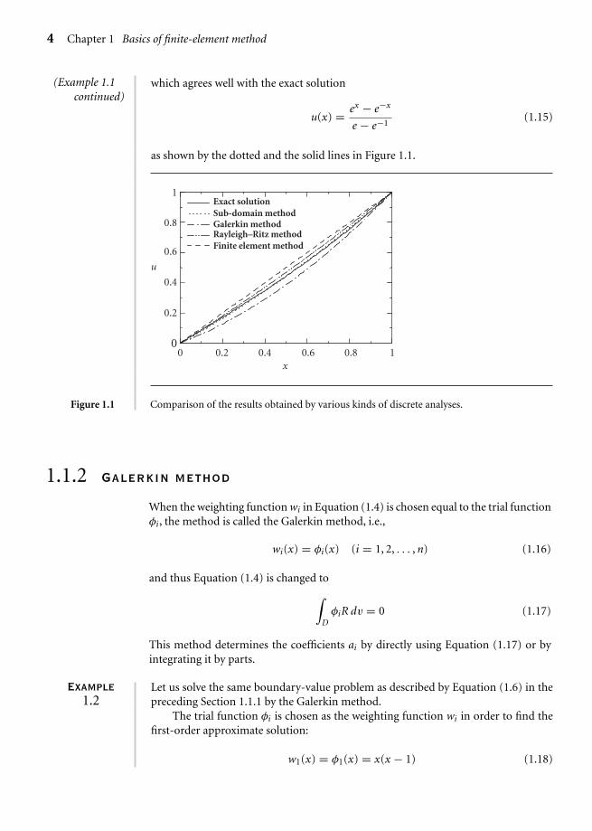
which agrees well with the exact solution

u(x) = ex − e−x

e − e−1(1.15)

as shown by the dotted and the solid lines in Figure 1.1.

0 0.2 0.4 0.6 0.8 10

0.2

0.4

0.6

0.8

1

x

u

Sub-domain methodExact solution

Galerkin methodRayleigh–Ritz methodFinite element method

Figure 1.1 Comparison of the results obtained by various kinds of discrete analyses.

1.1.2 Galerkin method

When the weighting function wi in Equation (1.4) is chosen equal to the trial functionφi, the method is called the Galerkin method, i.e.,

wi(x) = φi(x) (i = 1, 2, . . . , n) (1.16)

and thus Equation (1.4) is changed to∫D

φiR dv = 0 (1.17)

This method determines the coefficients ai by directly using Equation (1.17) or byintegrating it by parts.

Example1.2

Let us solve the same boundary-value problem as described by Equation (1.6) in thepreceding Section 1.1.1 by the Galerkin method.

The trial function φi is chosen as the weighting function wi in order to find thefirst-order approximate solution:

w1(x) = φ1(x) = x(x − 1) (1.18)

Ch01-H6875.tex 24/11/2006 17: 0 page 5

1.2 Rayleigh–Ritz method 5

(Example 1.2continued)

Integrating Equation (1.4) by parts,

∫ 1

0wiR dx =

∫ 1

0wi

(d2u

dx2− u

)dx =

[wi

du

dx

]1

0−

∫ 1

0

dwi

dx

du

dxdx −

∫ 1

0wiu dx = 0

(1.19)

is obtained. Choosing u1 in Equation (1.11) as the approximate solution u, thesubstitution of Equation (1.18) into (1.19) gives

∫ 1

0φ1R dx = −

∫ 1

0

dφ1

dx

du

dxdx −

∫ 1

0φ1u dx = −

∫ 1

0(2x − 1)[1 + A1(2x − 1)]dx

−∫ 1

0(x2 − x)[1 + A1(x2 − x)]dx = −A1

3+ 1

12− A1

30= 0 (1.20)

Thus, the following approximate solution is obtained:

u1(x) = x + 5

22x(x − 1) (1.21)

Figure 1.1 shows that the approximate solution obtained by the Galerkin method alsoagrees well with the exact solution throughout the region of interest.

1.2 Rayleigh–Ritz method

When there exists the functional which is equivalent to a given differential equation,the Rayleigh–Ritz method can be used.

Let us consider the example problem illustrated in Figure 1.2 where a particlehaving a mass of M slides from point P0 to lower point P1 along a curve in a verticalplane under the force of gravity. The time t that the particle needs for sliding fromthe points P0 to P1 varies with the shape of the curve denoted by y(x) which connectsthe two points. Namely, the time t can be considered as a kind of function t = F[y]which is determined by a function y(x) of an independent variable x. The function

P0

P1

M

y2(x)

y3(x)

y1(x)

y

x

Figure 1.2 Particle M sliding from point P0 to lower point P1 under gravitational force.

Ch01-H6875.tex 24/11/2006 17: 0 page 6


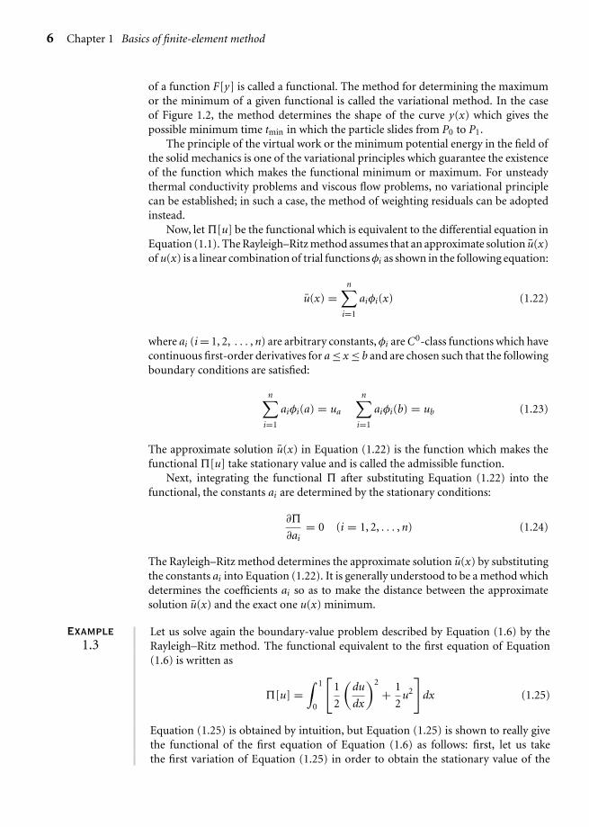
of a function F[y] is called a functional. The method for determining the maximumor the minimum of a given functional is called the variational method. In the caseof Figure 1.2, the method determines the shape of the curve y(x) which gives thepossible minimum time tmin in which the particle slides from P0 to P1.

The principle of the virtual work or the minimum potential energy in the field ofthe solid mechanics is one of the variational principles which guarantee the existenceof the function which makes the functional minimum or maximum. For unsteadythermal conductivity problems and viscous flow problems, no variational principlecan be established; in such a case, the method of weighting residuals can be adoptedinstead.

Now, let �[u] be the functional which is equivalent to the differential equation inEquation (1.1). The Rayleigh–Ritz method assumes that an approximate solution u(x)of u(x) is a linear combination of trial functions φi as shown in the following equation:

u(x) =n∑

i=1

aiφi(x) (1.22)

where ai (i = 1, 2, . . . , n) are arbitrary constants, φi are C0-class functions which havecontinuous first-order derivatives for a ≤ x ≤ b and are chosen such that the followingboundary conditions are satisfied:

n∑i=1

aiφi(a) = ua

n∑i=1

aiφi(b) = ub (1.23)

The approximate solution u(x) in Equation (1.22) is the function which makes thefunctional �[u] take stationary value and is called the admissible function.

Next, integrating the functional � after substituting Equation (1.22) into thefunctional, the constants ai are determined by the stationary conditions:

∂�

∂ai= 0 (i = 1, 2, . . . , n) (1.24)

The Rayleigh–Ritz method determines the approximate solution u(x) by substitutingthe constants ai into Equation (1.22). It is generally understood to be a method whichdetermines the coefficients ai so as to make the distance between the approximatesolution u(x) and the exact one u(x) minimum.

Example1.3

Let us solve again the boundary-value problem described by Equation (1.6) by theRayleigh–Ritz method. The functional equivalent to the first equation of Equation(1.6) is written as

�[u] =∫ 1

0

[1

2

(du

dx

)2

+ 1

2u2

]dx (1.25)

Equation (1.25) is obtained by intuition, but Equation (1.25) is shown to really givethe functional of the first equation of Equation (1.6) as follows: first, let us takethe first variation of Equation (1.25) in order to obtain the stationary value of the

Ch01-H6875.tex 24/11/2006 17: 0 page 7

1.3 Finite-element method 7

equation:

δ� =∫ 1

0

[du

dxδ

(du

dx

)+ uδu

]dx (1.26)

Then, integrating the above equation by parts, we have

δ� =∫ 1

0

(du

dx

dδu

dx+ uδu

)dx =

[du

dxδu

]1

0−∫ 1

0

[d

dx

(du

dx

)δu − uδu

]dx

= −∫ 1

0

(d2u

dx2− u

)δu dx (1.27)

For satisfying the stationary condition that δ� = 0, the rightmost-hand side ofEquation (1.27) should be identically zero over the interval considered (a ≤ x ≤ b),so that

d2u

dx2− u = 0 (1.28)

This is exactly the same as the first equation of Equation (1.6).Now, let us consider the following first-order approximate solution u1 which

satisfies the boundary conditions:

u1(x) = x + a1x(x − 1) (1.29)

Substitution of Equation (1.29) into (1.25) and integration of Equation (1.25)lead to

�[u1] =∫ 1

0

{1

2[1 + a1(2x − 1)]2 + 1

2

[x + a1(x2 − x)

]2}

dx = 2

3− 1

12a1 + 1

3a2

1

(1.30)

Since the stationary condition for Equation (1.30) is written by

∂�

∂a1= − 1

12+ 2

3a1 = 0 (1.31)

the first-order approximate solution can be obtained as follows:

u1(x) = x + 1

8x(x − 1) (1.32)

Figure 1.1 shows that the approximate solution obtained by the Rayleigh–Ritzmethod agrees well with the exact solution throughout the region considered.

1.3 Finite-element method

There are two ways for the formulation of the FEM: one is based on the directvariational method (such as the Rayleigh–Ritz method) and the other on the methodof weighted residuals (such as the Galerkin method). In the formulation based onthe variational method, the fundamental equations are derived from the stationaryconditions of the functional for the boundary-value problems. This formulationhas an advantage that the process of deriving functionals is not necessary, so it is

Ch01-H6875.tex 24/11/2006 17: 0 page 8


easy to formulate the FEM based on the method of the weighted residuals. In theformulation based on the variational method, however, it is generally difficult toderive the functional except for the case where the variational principles are alreadyestablished as in the case of the principle of the virtual work or the principle of theminimum potential energy in the field of the solid mechanics.

This section will explain how to derive the fundamental equations for the FEMbased on the Galerkin method.

Let us consider again the boundary-value problem stated by Equation (1.1):{L[u(x)] = f (x) (a ≤ x ≤ b)

BC (Boundary Conditions): u(a) = ua u(b) = ub

(1.33)

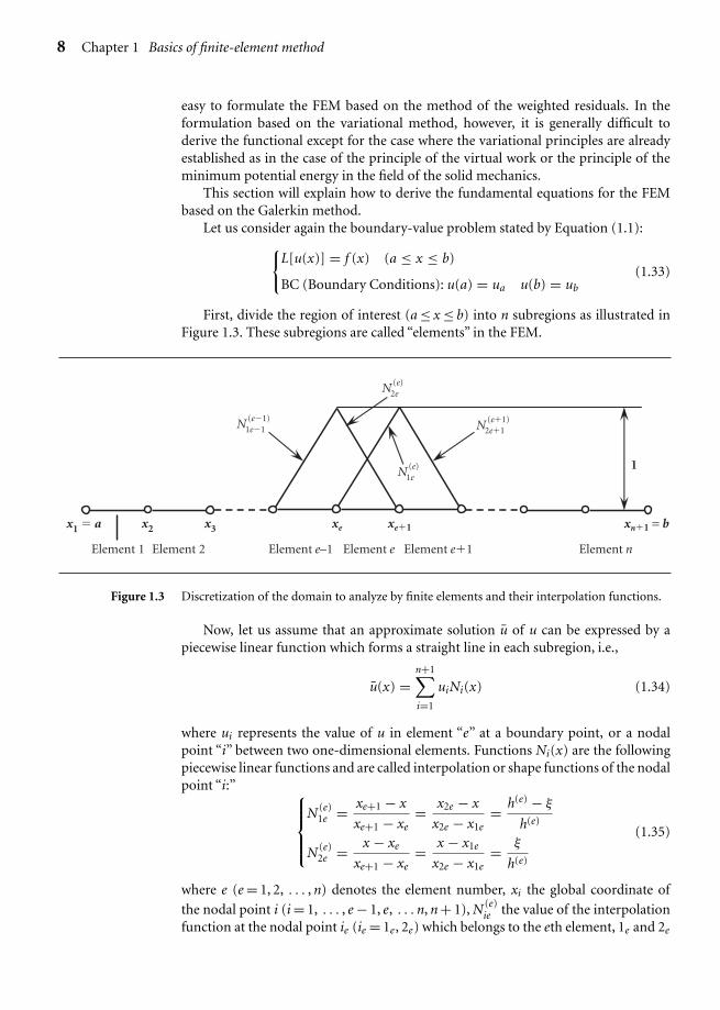
First, divide the region of interest (a ≤ x ≤ b) into n subregions as illustrated inFigure 1.3. These subregions are called “elements” in the FEM.

x1 � a x3 xe�1xe xn�1 = bx2

1

Element 1 Element 2 Element e–1 Element e Element e�1 Element n

(e�1)1e�1N (e�1)

2e�1N

(e)2eN

(e)1eN

Figure 1.3 Discretization of the domain to analyze by finite elements and their interpolation functions.

Now, let us assume that an approximate solution u of u can be expressed by apiecewise linear function which forms a straight line in each subregion, i.e.,

u(x) =n+1∑i=1

uiNi(x) (1.34)

where ui represents the value of u in element “e” at a boundary point, or a nodalpoint “i” between two one-dimensional elements. Functions Ni(x) are the followingpiecewise linear functions and are called interpolation or shape functions of the nodalpoint “i:” ⎧⎪⎪⎨

⎪⎪⎩N (e)

1e = xe+1 − x

xe+1 − xe= x2e − x

x2e − x1e= h(e) − ξ

h(e)

N (e)2e = x − xe

xe+1 − xe= x − x1e

x2e − x1e= ξ

h(e)

(1.35)

where e (e = 1, 2, . . . , n) denotes the element number, xi the global coordinate of

the nodal point i (i = 1, . . . , e − 1, e, . . . n, n + 1), N (e)ie the value of the interpolation

function at the nodal point ie (ie = 1e , 2e) which belongs to the eth element, 1e and 2e

Ch01-H6875.tex 24/11/2006 17: 0 page 9


the number of two nodal points of the eth element. Symbol ξ is the local coordinateof an arbitrary point in the eth element, ξ = x − xe = x − x1e (0 ≤ ξ ≤ h(e)), h(e) is thelength of the eth element, and h(e) is expressed as h(e) = xe+1 − xe = x2e − x1e .

As the interpolation function, the piecewise linear or quadric function is oftenused. Generally speaking, the quadric interpolation function gives better solutionsthan the linear one.

The Galerkin method-based FEM adopts the weighting functions wi(x) equal tothe interpolation functions Ni(x), i.e.,

wi(x) = Ni(x) (i = 1, 2, . . . , n + 1) (1.36)

Thus, Equation (1.4) becomes ∫D

NiR dv = 0 (1.37)

In the FEM, a set of simultaneous algebraic equations for unknown variables ofu(x) at the ith nodal point ui and those of its derivatives du/dx, (du/dx)i are derivedby integrating Equation (1.37) by parts and then by taking boundary conditions intoconsideration. The simultaneous equations can be easily solved by digital computersto determine the unknown variables ui and (du/dx)i at all the nodal points in theregion considered.

Example1.4

Let us solve the boundary-value problem stated in Equation (1.6) by FEM.First, the integration of Equation (1.37) by parts gives

∫ 1

0wiR dx =

∫ 1

0wi

(d2u

dx2− u

)dx =

[wi

du

dx

]1

0−∫ 1

0

(dwi

dx

du

dx+ wiu

)dx = 0

(i = 1, 2, . . . , n + 1) (1.38)

Then, the substitution of Equations (1.34) and (1.36) into Equation (1.38) gives

n+1∑j=1

∫ 1

0

(dNi

dx

dNj

dx+ NiNj

)ujdx −

[Ni

du

dx

]1

0= 0 (i = 1, 2, . . . , n + 1) (1.39)

Equation (1.39) is a set of simultaneous linear algebraic equations composed of(n + 1) nodal values ui of the solution u and also (n + 1) nodal values (du/dx)i of itsderivative du/dx. The matrix notation of the simultaneous equations above is writtenin a simpler form as follows:

[Kij]{uj} = {fi} (1.40)

where [Kij] is a square matrix of (n + 1) by (n + 1), {fi} is a column vector of (n + 1)by 1, and the components of the matrix and the vector Kij and fi are expressed as⎧⎪⎪⎪⎨

⎪⎪⎪⎩Kij ≡

∫ 1

0

(dNi

dx

dNj

dx+ NiNj

)dx (1 ≤ i, j ≤ n + 1)

fi ≡[

Nidu

dx

]1

0(1 ≤ i ≤ n + 1)

(1.41)

Ch01-H6875.tex 24/11/2006 17: 0 page 10


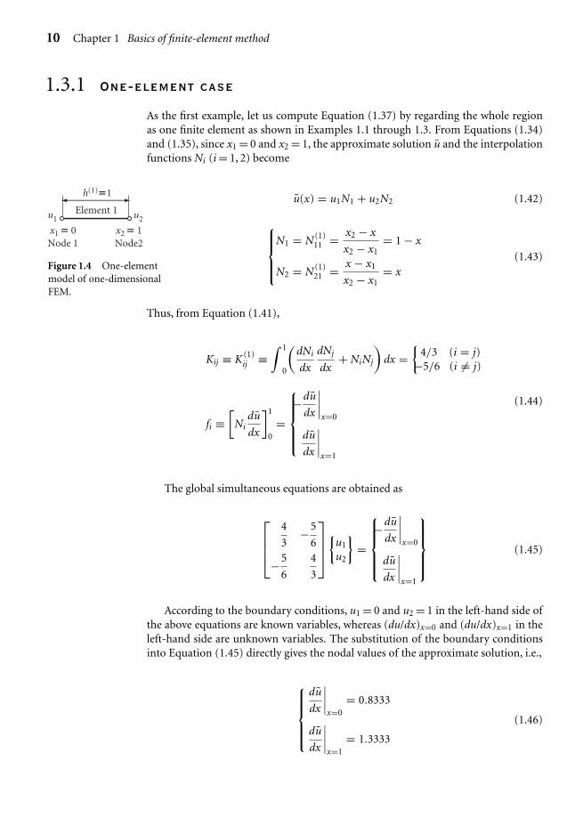
1.3.1 One-element case

As the first example, let us compute Equation (1.37) by regarding the whole regionas one finite element as shown in Examples 1.1 through 1.3. From Equations (1.34)and (1.35), since x1 = 0 and x2 = 1, the approximate solution u and the interpolationfunctions Ni (i = 1, 2) become

Element 1u1 u2

h(1)�1

x1 � 0Node 1

x2 � 1Node2

Figure 1.4 One-elementmodel of one-dimensionalFEM.

u(x) = u1N1 + u2N2 (1.42)

⎧⎪⎪⎨⎪⎪⎩

N1 = N (1)11 = x2 − x

x2 − x1= 1 − x

N2 = N (1)21 = x − x1

x2 − x1= x

(1.43)

Thus, from Equation (1.41),

Kij ≡ K (1)ij ≡

∫ 1

0

(dNi

dx

dNj

dx+ NiNj

)dx =

{4/3 (i = j)

−5/6 (i �= j)

fi ≡[

Nidu

dx

]1

0=

⎧⎪⎪⎪⎨⎪⎪⎪⎩−du

dx

∣∣∣∣x=0

du

dx

∣∣∣∣x=1

(1.44)

The global simultaneous equations are obtained as

⎡⎢⎢⎣

4

3−5

6

−5

6

4

3

⎤⎥⎥⎦{

u1

u2

}=

⎧⎪⎪⎪⎨⎪⎪⎪⎩−du

dx

∣∣∣∣x=0

du

dx

∣∣∣∣x=1

⎫⎪⎪⎪⎬⎪⎪⎪⎭

(1.45)

According to the boundary conditions, u1 = 0 and u2 = 1 in the left-hand side ofthe above equations are known variables, whereas (du/dx)x=0 and (du/dx)x=1 in theleft-hand side are unknown variables. The substitution of the boundary conditionsinto Equation (1.45) directly gives the nodal values of the approximate solution, i.e.,

⎧⎪⎪⎪⎨⎪⎪⎪⎩

du

dx

∣∣∣∣x=0

= 0.8333

du

dx

∣∣∣∣x=1

= 1.3333

(1.46)

Ch01-H6875.tex 24/11/2006 17: 0 page 11


which agrees well with those of the exact solution

⎧⎪⎪⎨⎪⎪⎩

du

dx

∣∣∣∣x=0

= 2

e − e−1= 0.8509

du

dx

∣∣∣∣x=1

= e + e−1

e − e−1= 1.3130

(1.47)

The approximate solution in this example is determined as

u(x) = x (1.48)

and agrees well with the exact solution throughout the whole region of interest asdepicted in Figure 1.1.

1.3.2 Three-element case

In this section, let us compute the approximate solution u by dividing the wholeregion considered into three subregions having the same length as shown in Figure 1.5.From Equations (1.34) and (1.35), the approximate solution u and the interpolationfunctions Ni (i = 1, 2) are written as

u(x) =4∑

i=1

uiNi (1.49)

⎧⎪⎪⎪⎨⎪⎪⎪⎩

N1e = x2e − x

x2e − x1e= h(e) − ξ

h(e)

N2e = x − x1e

x2e − x1e= ξ

h(e)

(1.50)

where h(e) = 1/3 and 0 ≤ ξ ≤ 1/3 (e = 1, 2, 3).

Element 1u1 u2

h(1) = 1/3

x1 = 0Node 1

Element 2 u3

h(2) = 1/3

x2 = 1/3Node 2

x3 = 1/3Node 3

Element 3 u4

h(3) = 1/3

x4 = 1/3Node 4

Figure 1.5 Three-element model of a one-dimensional FEM.

Ch01-H6875.tex 24/11/2006 17: 0 page 12


By calculating all the components of the K-matrix in Equation (1.41), thefollowing equation is obtained:

K (e)ij ≡

∫ 1

0

⎛⎝dN (e)

i

dx

dN (e)j

dx+ N (e)

i N (e)j

⎞⎠ dx

=

⎧⎪⎪⎪⎪⎪⎪⎨⎪⎪⎪⎪⎪⎪⎩

1

h(e)+ h(e)

3= 28

9(i = j and i, j = 1e, 2e)

− 1

h(e)+ h(e)

6= −53

18(i �= j and i, j = 1e, 2e)

0 (i, j �= 1e, 2e)

(1.51a)

The components relating to the first derivative of the function u in Equation (1.41)are calculated as follows:

fi ≡[

Nidu

dx

]1

0=

⎧⎪⎪⎪⎪⎪⎨⎪⎪⎪⎪⎪⎩

−du

dx

∣∣∣∣x=0

(i = 1)

0 (i = 2, 3)

du

dx

∣∣∣∣x=1

(i = 4)

(1.51b)

The coefficient matrix in Equation (1.51a) calculated for each element is called“element matrix” and the components of the matrix are obtained as follows:

[K (1)

ij

]=

⎡⎢⎢⎢⎢⎢⎢⎢⎢⎣

1

h(1)+ h(1)

3− 1

h(1)+ h(1)

60 0

− 1

h(1)+ h(1)

6

1

h(1)+ h(1)

30 0

0 0 0 0

0 0 0 0

⎤⎥⎥⎥⎥⎥⎥⎥⎥⎦

(1.52a)

[K (2)

ij

]=

⎡⎢⎢⎢⎢⎢⎢⎢⎢⎣

0 0 0 0

01

h(2)+ h(2)

3− 1

h(2)+ h(2)

60

0 − 1

h(2)+ h(2)

6

1

h(2)+ h(2)

30

0 0 0 0

⎤⎥⎥⎥⎥⎥⎥⎥⎥⎦

(1.52b)

[K (3)

ij

]=

⎡⎢⎢⎢⎢⎢⎢⎢⎢⎢⎢⎣

0 0 0 0

0 0 0 0

0 01

h(3)+ h(3)

3− 1

h(3)+ h(3)

6

0 0 − 1

h(3)+ h(3)

6

1

h(3)+ h(3)

3

⎤⎥⎥⎥⎥⎥⎥⎥⎥⎥⎥⎦

(1.52c)

Ch01-H6875.tex 24/11/2006 17: 0 page 13


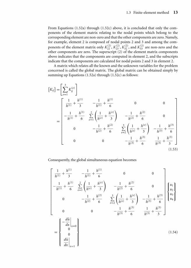
From Equations (1.52a) through (1.52c) above, it is concluded that only the com-ponents of the element matrix relating to the nodal points which belong to thecorresponding element are non-zero and that the other components are zero. Namely,for example, element 2 is composed of nodal points 2 and 3 and among the com-

ponents of the element matrix only K (2)22 , K (2)

23 , K (2)32 , and K (2)

33 are non-zero and theother components are zero. The superscript (2) of the element matrix componentsabove indicates that the components are computed in element 2, and the subscriptsindicate that the components are calculated for nodal points 2 and 3 in element 2.

A matrix which relates all the known and the unknown variables for the problemconcerned is called the global matrix. The global matrix can be obtained simply bysumming up Equations (1.52a) through (1.52c) as follows:

[Kij

] =[

3∑e=1

K (e)ij

]

=

⎡⎢⎢⎢⎢⎢⎢⎢⎢⎢⎢⎢⎢⎢⎢⎣

1

h(1)+ h(1)

3− 1

h(1)+ h(1)

60 0

− 1

h(1)+ h(1)

6

2∑e=1

(1

h(e)+ h(e)

3

)− 1

h(2)+ h(2)

60

0 − 1

h(2)+ h(2)

6

3∑e=2

(1

h(e)+ h(e)

3

)− 1

h(3)+ h(3)

6

0 0 − 1

h(3)+ h(3)

6

1

h(3)+ h(3)

3

⎤⎥⎥⎥⎥⎥⎥⎥⎥⎥⎥⎥⎥⎥⎥⎦

(1.53)

Consequently, the global simultaneous equation becomes

⎡⎢⎢⎢⎢⎢⎢⎢⎢⎢⎢⎢⎢⎢⎢⎣

1

h(1)+ h(1)

3− 1

h(1)+ h(1)

60 0

− 1

h(1)+ h(1)

6

2∑e=1

(1

h(e)+ h(e)

3

)− 1

h(2)+ h(2)

60

0 − 1

h(2)+ h(2)

6

3∑e=2

(1

h(e)+ h(e)

3

)− 1

h(3)+ h(3)

6

0 0 − 1

h(3)+ h(3)

6

1

h(3)+ h(3)

3

⎤⎥⎥⎥⎥⎥⎥⎥⎥⎥⎥⎥⎥⎥⎥⎦

⎧⎪⎪⎨⎪⎪⎩

u1

u2

u3

u4

⎫⎪⎪⎬⎪⎪⎭

=

⎧⎪⎪⎪⎪⎪⎪⎨⎪⎪⎪⎪⎪⎪⎩

−du

dx

∣∣∣∣x=0

0

0du

dx

∣∣∣∣x=1

⎫⎪⎪⎪⎪⎪⎪⎬⎪⎪⎪⎪⎪⎪⎭

(1.54)

Ch01-H6875.tex 24/11/2006 17: 0 page 14


Note that the coefficient matrix [Kij] in the left-hand side of Equation (1.54) issymmetric with respect to the non-diagonal components (i �= j), i.e., Kij = Kji. Onlythe components in the band region around the diagonal of the matrix are non-zeroand the others are zero. Due to this nature, the coefficient matrix is called the sparseor band matrix.

From the boundary conditions, the values of u1 and u4 in the left-hand side ofEquation (1.54) are known, i.e., u1 = 0 and u4 = 1 and, from Equation (1.51b), thevalues of f2 and f3 in the right-hand side are also known, i.e., f2 = 0 and f3 = 0. On the

other hand, u2 and u3 in the left-hand side and dudx

∣∣∣x=0

and dudx

∣∣∣x=1

in the right-hand

side are unknown variables. By changing unknown variables dudx

∣∣∣x=0

and dudx

∣∣∣x=1

with

the first and the fourth components of the vector in the left-hand side of Equation(1.54) and by substituting h(1) = h(2) = h(3) = 1/3 into Equation (1.54), after rear-rangement of the equation, the global simultaneous equation is rewritten as follows:

⎡⎢⎢⎢⎢⎢⎢⎢⎢⎢⎢⎣

−1 −53

180 0

056

9−53

180

0 −53

18

56

90

0 0 −53

18−1

⎤⎥⎥⎥⎥⎥⎥⎥⎥⎥⎥⎦

⎧⎪⎪⎪⎪⎪⎪⎪⎪⎪⎨⎪⎪⎪⎪⎪⎪⎪⎪⎪⎩

dudx

∣∣∣x=0

u2

u3

dudx

∣∣∣x=1

⎫⎪⎪⎪⎪⎪⎪⎪⎪⎪⎬⎪⎪⎪⎪⎪⎪⎪⎪⎪⎭

=

⎧⎪⎪⎪⎪⎪⎪⎪⎪⎪⎨⎪⎪⎪⎪⎪⎪⎪⎪⎪⎩

0

0

53

18

−28

9

⎫⎪⎪⎪⎪⎪⎪⎪⎪⎪⎬⎪⎪⎪⎪⎪⎪⎪⎪⎪⎭

(1.55)

where the new vector in the left-hand side of the equation is an unknown vector andthe one in the right-hand side is a known vector.

After solving Equation (1.55), it is found that u2 = 0.2885, u3 = 0.6098,dudx

∣∣∣x=0

= 0.8496, and dudx

∣∣∣x=1

= 1.3157. The exact solutions for u2 and u3 can be

calculated as u2 = 0.2889 and u3 = 0.6102 from Equation (1.55). The relative errorsfor u2 and u3 are as small as 0.1% and 0.06%, respectively. The calculated values

of the derivative dudx

∣∣∣x=0

and dudx

∣∣∣x=1

are improved when compared to those by the

one-element FEM described in Section 1.3.1.In this section, only one-dimensional FEM was described. The FEM can be applied

to two- and three-dimensional continuum problems of various kinds which aredescribed in terms of ordinary and partial differential equations. There is no essen-tial difference between the formulation for one-dimensional problems and theformulations for higher dimensions except for the intricacy of formulation.

1.4 FEM in two-dimensional elastostaticproblems

Generally speaking, elasticity problems are reduced to solving the partial differen-tial equations known as the equilibrium equations together with the stress–strainrelations or the constitutive equations, the strain–displacement relations, and the

Ch01-H6875.tex 24/11/2006 17: 0 page 15

1.4 FEM in two-dimensional elastostatic problems 15

compatibility equation under given boundary conditions. The exact solutions can beobtained in quite limited cases only and in general cannot be solved in closed forms.In order to overcome these difficulties, the FEM has been developed as one of thepowerful numerical methods to obtain approximate solutions for various kinds ofelasticity problems. The FEM assumes an object of analysis as an aggregate of ele-ments having arbitrary shapes and finite sizes (called finite element), approximatespartial differential equations by simultaneous algebraic equations, and numericallysolves various elasticity problems. Finite elements take the form of line segment inone-dimensional problems as shown in the preceding section, triangle or rectangle intwo-dimensional problems, and tetrahedron, cuboid, or prism in three-dimensionalproblems. Since the procedure of the FEM is mathematically based on the variationalmethod, it can be applied not only to elasticity problems of structures but also tovarious problems related to thermodynamics, fluid dynamics, and vibrations whichare described by partial differential equations.

1.4.1 Elements of finite-element procedures in the analysisof plane elastostatic problems

Limited to static (without time variation) elasticity problems, the procedure describedin the preceding section is essentially the same as that of the stress analyses by the FEM.

The procedure is summarized as follows:

• Procedure 1: Discretization Divide the object of analysis into a finite number offinite elements.

• Procedure 2: Selection of the interpolation function Select the element type orthe interpolation function which approximates displacements and strains in eachfinite element.

• Procedure 3: Derivation of element stiffness matrices Determine the elementstiffness matrix which relates forces and displacements in each element.

• Procedure 4: Assembly of stiffness matrices into the global stiffness matrix Assem-ble the element stiffness matrices into the global stiffness matrix which relatesforces and displacements in the whole elastic body to be analyzed.

• Procedure 5: Rearrangement of the global stiffness matrix Substitute prescribedapplied forces (mechanical boundary conditions) and displacements (geometricalboundary conditions) into the global stiffness matrix, and rearrange the matrixby collecting unknown variables for forces and displacements, say in the left-handside, and known values of the forces and displacements in the right-hand side inorder to set up simultaneous equations.

• Procedure 6: Derivation of unknown forces and displacements Solve the simulta-neous equations set up in Procedure 5 above to solve the unknown variables forforces and displacements. The solutions for unknown forces are reaction forcesand those for unknown displacements are deformations of the elastic body ofinterest for given geometrical and mechanical boundary conditions, respectively.

• Procedure 7: Computation of strains and stresses Compute the strains and stressesfrom the displacements obtained in Procedure 6 by using the strain–displacementrelations and the stress–strain relations explained later.

Ch01-H6875.tex 24/11/2006 17: 0 page 16


1.4.2 Fundamental formulae in plane elastostatic problems

1.4.2.1 EQUATIONS OF EQUILIBRIUM

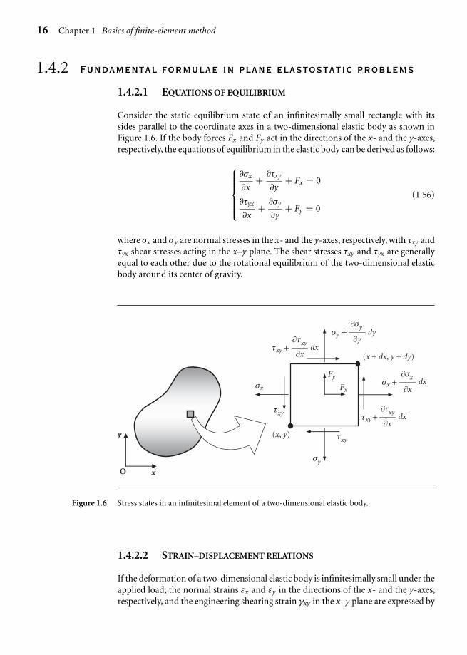
Consider the static equilibrium state of an infinitesimally small rectangle with itssides parallel to the coordinate axes in a two-dimensional elastic body as shown inFigure 1.6. If the body forces Fx and Fy act in the directions of the x- and the y-axes,respectively, the equations of equilibrium in the elastic body can be derived as follows:

⎧⎪⎪⎪⎨⎪⎪⎪⎩

∂σx

∂x+ ∂τxy

∂y+ Fx = 0

∂τyx

∂x+ ∂σy

∂y+ Fy = 0

(1.56)

where σx and σy are normal stresses in the x- and the y-axes, respectively, with τxy andτyx shear stresses acting in the x–y plane. The shear stresses τxy and τyx are generallyequal to each other due to the rotational equilibrium of the two-dimensional elasticbody around its center of gravity.

x

y

O

(x + dx, y + dy)

(x, y)

dx∂x

∂τxy+τxy

dy∂y

∂σy+σy

dx∂x

∂σx+σx

dx∂x

∂τxy+τxy

τxy

τxy

σx

σy

Fy

Fx

Figure 1.6 Stress states in an infinitesimal element of a two-dimensional elastic body.

1.4.2.2 STRAIN–DISPLACEMENT RELATIONS

If the deformation of a two-dimensional elastic body is infinitesimally small under theapplied load, the normal strains εx and εy in the directions of the x- and the y-axes,respectively, and the engineering shearing strain γxy in the x–y plane are expressed by

Ch01-H6875.tex 24/11/2006 17: 0 page 17


the following equations: ⎧⎪⎪⎪⎪⎪⎪⎨⎪⎪⎪⎪⎪⎪⎩

εx = ∂u

∂x

εy = ∂v

∂y

γxy = ∂v

∂x+ ∂u

∂y

(1.57)

where u and v are infinitesimal displacements in the directions of the x- and they-axes, respectively.

1.4.2.3 STRESS–STRAIN RELATIONS (CONSTITUTIVE EQUATIONS)

The stress–strain relations describe states of deformation, strains induced by the inter-nal forces, or stresses resisting against applied loads. Unlike the other fundamentalequations shown in Equations (1.56) and (1.57) which can be determined mecha-nistically or geometrically, these relations depend on the properties of the material,and they are determined experimentally and often called constitutive relations orconstitutive equations. One of the most popular relations is the generalized Hooke’slaw which relates six components of the three-dimensional stress tensor with thoseof strain tensor through the following simple linear expressions:⎧⎪⎪⎪⎪⎪⎪⎪⎪⎪⎪⎪⎪⎪⎪⎪⎪⎪⎪⎪⎨

⎪⎪⎪⎪⎪⎪⎪⎪⎪⎪⎪⎪⎪⎪⎪⎪⎪⎪⎪⎩

σx = νE

(1 + ν) (1 − 2ν)ev + 2Gεx

σy = νE

(1 + ν) (1 − 2ν)ev + 2Gεy

σy = νE

(1 + ν) (1 − 2ν)ev + 2Gεz

τxy = Gγxy = E

2 (1 + ν)γxy

τyz = Gγyz = E

2 (1 + ν)γyz

τzx = Gγzx = E

2 (1 + ν)γzx

(1.58a)

or inversely ⎧⎪⎪⎪⎪⎪⎪⎪⎪⎪⎪⎪⎪⎪⎪⎪⎪⎪⎪⎪⎨⎪⎪⎪⎪⎪⎪⎪⎪⎪⎪⎪⎪⎪⎪⎪⎪⎪⎪⎪⎩

εx = 1

E

[σx − ν

(σy + σz

)]εy = 1

E

[σy − ν (σz + σx)

]εz = 1

E

[σz − ν

(σx + σy

)]γxy = τxy

G

γyz = τyz

G

γzx = τzx

G

(1.58b)

Ch01-H6875.tex 24/11/2006 17: 0 page 18


where E is Young’s modulus, ν Poisson’s ratio, G the shear modulus, and ev thevolumetric strain expressed by the sum of the three normal components of strain,i.e., ev = εx + εy + εz . The volumetric strain ev can be written in other words asev = �V /V , where V is the initial volume of the elastic body of interest in anundeformed state and �V the change of the volume after deformation.

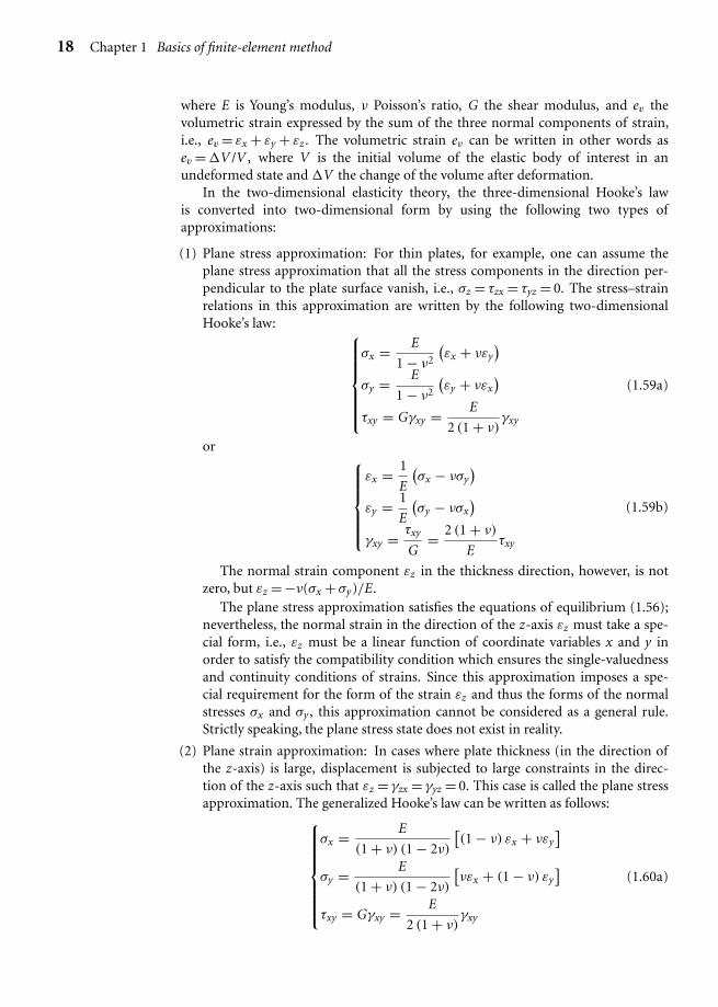
In the two-dimensional elasticity theory, the three-dimensional Hooke’s lawis converted into two-dimensional form by using the following two types ofapproximations:

(1) Plane stress approximation: For thin plates, for example, one can assume theplane stress approximation that all the stress components in the direction per-pendicular to the plate surface vanish, i.e., σz = τzx = τyz = 0. The stress–strainrelations in this approximation are written by the following two-dimensionalHooke’s law: ⎧⎪⎪⎪⎪⎪⎨

⎪⎪⎪⎪⎪⎩

σx = E

1 − ν2

(εx + νεy

)σy = E

1 − ν2

(εy + νεx

)τxy = Gγxy = E

2 (1 + ν)γxy

(1.59a)

or ⎧⎪⎪⎪⎪⎨⎪⎪⎪⎪⎩

εx = 1

E

(σx − νσy

)εy = 1

E

(σy − νσx

)γxy = τxy

G= 2 (1 + ν)

Eτxy

(1.59b)

The normal strain component εz in the thickness direction, however, is notzero, but εz = −ν(σx + σy)/E.

The plane stress approximation satisfies the equations of equilibrium (1.56);nevertheless, the normal strain in the direction of the z-axis εz must take a spe-cial form, i.e., εz must be a linear function of coordinate variables x and y inorder to satisfy the compatibility condition which ensures the single-valuednessand continuity conditions of strains. Since this approximation imposes a spe-cial requirement for the form of the strain εz and thus the forms of the normalstresses σx and σy , this approximation cannot be considered as a general rule.Strictly speaking, the plane stress state does not exist in reality.

(2) Plane strain approximation: In cases where plate thickness (in the direction ofthe z-axis) is large, displacement is subjected to large constraints in the direc-tion of the z-axis such that εz = γzx = γyz = 0. This case is called the plane stressapproximation. The generalized Hooke’s law can be written as follows:⎧⎪⎪⎪⎪⎪⎪⎨

⎪⎪⎪⎪⎪⎪⎩

σx = E

(1 + ν) (1 − 2ν)

[(1 − ν) εx + νεy

]σy = E

(1 + ν) (1 − 2ν)

[νεx + (1 − ν) εy

]τxy = Gγxy = E

2 (1 + ν)γxy

(1.60a)

Ch01-H6875.tex 24/11/2006 17: 0 page 19


or ⎧⎪⎪⎪⎪⎪⎨⎪⎪⎪⎪⎪⎩

εx = 1 + ν

E

[(1 − ν) σx − νσy

]εy = 1 + ν

E

[−νσx + (1 − ν) σy]

γxy = τxy

G= 2 (1 + ν)

Eτxy

(1.60b)

The normal stress component σz in the thickness direction is not zero, butσz = νE(σx + σy)/[(1 + ν) (1 − 2ν)]. Since the plane strain state satisfies the equa-tions of equilibrium (1.56) and the compatibility condition, this state can exist inreality.

If we redefine Young’s modulus and Poisson’s ratio by the following formulae:

E′ =⎧⎨⎩

E (plane stress)

E

1 − ν(plane strain)

(1.61a)

ν′ =⎧⎨⎩

ν (plane stress)ν

1 − ν(plane strain)

(1.61b)

the two-dimensional Hooke’s law can be expressed in a unified form:⎧⎪⎪⎪⎪⎪⎪⎨⎪⎪⎪⎪⎪⎪⎩

σx = E′

1 − ν′2(εx + ν′εy

)σy = E′

1 − ν′2(εy + ν′εx

)τxy = Gγxy = E′

2 (1 + ν′)γxy

(1.62a)

or ⎧⎪⎪⎪⎪⎪⎪⎨⎪⎪⎪⎪⎪⎪⎩

εx = 1

E′(σx − ν′σy

)εy = 1

E′(σy − ν′σx

)γxy = τxy

G= 2

(1 + ν′)

E′ τxy

(1.62b)

The shear modulus G is invariant under the transformations as shown inEquations (1.61a) and (1.61b), i.e.,

G = E

2(1 + ν)= E′

2(1 + ν′)= G′

1.4.2.4 BOUNDARY CONDITIONS

When solving the partial differential equation (1.56), there remains indefiniteness inthe form of integral constants. In order to eliminate this indefiniteness, prescribed

Ch01-H6875.tex 24/11/2006 17: 0 page 20


conditions on stress and/or displacements must be imposed on the bounding surfaceof the elastic body. These conditions are called boundary conditions. There are twotypes of boundary conditions, i.e. (1) mechanical boundary conditions prescribingstresses or surface tractions and (2) geometrical boundary conditions prescribingdisplacements.

Let us denote a portion of the surface of the elastic body where stresses areprescribed by Sσ and the remaining surface where displacements are prescribed bySu. The whole surface of the elastic body is denoted by S = Sσ + Su. Note that it is notpossible to prescribe both stresses and displacements on a portion of the surface ofthe elastic body.

The mechanical boundary conditions on Sσ are given by the following equations:{t∗x = t∗

x

t∗y = t∗

y(1.63)

where t∗x and t∗

y are the x- and the y-components of the traction force t*, respectively,while the bar over t∗

x and t∗y indicates that those quantities are prescribed on that

portion of the surface. Taking n = [cos α, sin α] as the outward unit normal vectorat a point of a small element of the surface portion Sσ , the Cauchy relations whichrepresent the equilibrium conditions for surface traction forces and internal stressesare given by the following equations:{

t∗x = σx cos α + τxy sin α

t∗y = τxy cos α + σy sin α

(1.64)

where α is the angle between the normal vector n and the x-axis. For free surfaceswhere no forces are applied, t∗

x = 0 and t∗y = 0.

Su

Ss

D

e

1e

2e

3e

Figure 1.7 Finite-element discretization of a two-dimensional elastic body by triangular elements.

Ch01-H6875.tex 24/11/2006 17: 0 page 21


The geometrical boundary conditions on Su are given by the following equations:

{u = uv = v

(1.65)

where u and v are the x- and the y-components of prescribed displacements u onSu. One of the most popular geometrical boundary conditions, i.e., clamped endcondition, is denoted by u = 0 and/or v = 0 as shown in Figure 1.7.

1.4.3 Variational formulae in elastostatic problems:the principle of virtual work

The variational principle used in two-dimensional elasticity problems is the principleof virtual work which is expressed by the following integral equation:

∫∫D

(σxδεx + σyδεy + τxyδγxy

)t dx dy−

∫∫D

(Fxδu + Fyδv

)t dx dy

−∫Sσ

(t∗

xδu + t∗yδv

)t ds = 0 (1.66)

where D denotes the whole region of a two-dimensional elastic body of interest,Sσ the whole portion of the surface of the elastic body S(=Sσ ∪ Su), where themechanical boundary conditions are prescribed and t the thickness.

The first term in the left-hand side of Equation (1.66) represents the incrementof the strain energy of the elastic body, the second term the increment of the workdone by the body forces, and the third term the increment of the work done by thesurface traction forces. Therefore, Equation (1.66) claims that the increment of thestrain energy of the elastic body is equal to the work done by the forces applied.

The fact that the integrand in each integral in the left-hand side of Equation(1.66) is identically equal to zero brings about the equations of equilibrium (1.56)and the boundary conditions (1.63) and/or (1.65). Therefore, instead of solving thepartial differential equations (1.56) under the boundary conditions of Equations(1.63) and/or (1.65), two-dimensional elasticity problems can be solved by using theintegral equation (1.66).

1.4.4 Formulation of the fundamental finite-element equationsin plane elastostatic problems

1.4.4.1 STRAIN–DISPLACEMENT MATRIX OR [B] MATRIX

Let us use the constant-strain triangular element (see Figure 1.8(a)) to derive the fun-damental finite-element equations in plane elastostatic problems. The constant-straintriangular element assumes the displacements within the element to be expressed by

Ch01-H6875.tex 24/11/2006 17: 0 page 22


2e

3e

(a)

1e

∆(e)

(b)

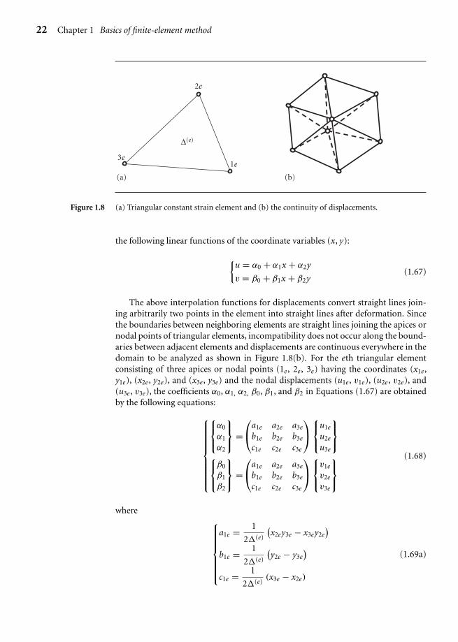
Figure 1.8 (a) Triangular constant strain element and (b) the continuity of displacements.

the following linear functions of the coordinate variables (x, y):

{u = α0 + α1x + α2y

v = β0 + β1x + β2y(1.67)

The above interpolation functions for displacements convert straight lines join-ing arbitrarily two points in the element into straight lines after deformation. Sincethe boundaries between neighboring elements are straight lines joining the apices ornodal points of triangular elements, incompatibility does not occur along the bound-aries between adjacent elements and displacements are continuous everywhere in thedomain to be analyzed as shown in Figure 1.8(b). For the eth triangular elementconsisting of three apices or nodal points (1e , 2e , 3e) having the coordinates (x1e ,y1e), (x2e , y2e), and (x3e , y3e) and the nodal displacements (u1e , v1e), (u2e , v2e), and(u3e , v3e), the coefficients α0, α1, α2, β0, β1, and β2 in Equations (1.67) are obtainedby the following equations:

⎧⎪⎪⎪⎪⎪⎪⎪⎨⎪⎪⎪⎪⎪⎪⎪⎩

⎧⎨⎩

α0

α1

α2

⎫⎬⎭ =

⎛⎝a1e a2e a3e

b1e b2e b3e

c1e c2e c3e

⎞⎠

⎧⎨⎩

u1e

u2e

u3e

⎫⎬⎭

⎧⎨⎩

β0

β1

β2

⎫⎬⎭ =

⎛⎝a1e a2e a3e

b1e b2e b3e

c1e c2e c3e

⎞⎠

⎧⎨⎩

v1e

v2e

v3e

⎫⎬⎭

(1.68)

where ⎧⎪⎪⎪⎪⎪⎨⎪⎪⎪⎪⎪⎩

a1e = 1

2�(e)

(x2ey3e − x3ey2e

)b1e = 1

2�(e)

(y2e − y3e

)c1e = 1

2�(e)(x3e − x2e)

(1.69a)

Ch01-H6875.tex 24/11/2006 17: 0 page 23


⎧⎪⎪⎪⎪⎪⎨⎪⎪⎪⎪⎪⎩

a2e = 1

2�(e)

(x3ey1e − x1ey3e

)b2e = 1

2�(e)

(y3e − y1e

)c2e = 1

2�(e)(x1e − x3e)

(1.69b)

⎧⎪⎪⎪⎪⎪⎨⎪⎪⎪⎪⎪⎩

a3e = 1

2�(e)

(x1ey2e − x2ey1e

)b3e = 1

2�(e)

(y1e − y2e

)c3e = 1

2�(e)(x2e − x1e)

(1.69c)

The numbers with subscript “e”, 1e , 2e , and 3e , in the above equations are calledelement nodal numbers and denote the numbers of three nodal points of the ethelement. Nodal points should be numbered counterclockwise. These three numbersare used only in the eth element. Nodal numbers of the other type called global nodalnumbers are also assigned to the three nodal points of the eth element, being num-bered throughout the whole model of the elastic body. The symbol �(e) representsthe area of the eth element and can be expressed only by the coordinates of the nodalpoints of the element, i.e.,

�(e) = 1

2

[(x1e − x3e)

(y2e − y3e

) − (y3e − y1e

)(x3e − x2e)

] = 1

2

∣∣∣∣∣∣1 x1e y1e

1 x2e y2e

1 x3e y3e

∣∣∣∣∣∣(1.69d)

Consequently, the components of the displacement vector [u, v] can be expressed bythe components of the nodal displacement vectors [u1e , v1e], [u2e , v2e], and [u3e , v3e]as follows:

⎧⎨⎩

u = (a1e + b1ex + c1ey

)u1e + (

a2e + b2ex + c2ey)

u2e + (a3e + b3ex + c3ey

)u3e

v = (a1e + b1ex + c1ey

)v1e + (

a2e + b2ex + c2ey)v2e + (

a3e + b3ex + c3ey)v3e

(1.70)Matrix notation of Equation (1.70) is

{uv

}=

[N (e)

1e 0 N (e)2e 0 N (e)

3e 0

0 N (e)1e 0 N (e)

2e 0 N (e)3e

]⎧⎪⎪⎪⎪⎪⎪⎨⎪⎪⎪⎪⎪⎪⎩

u1e

v1e

u2e

v2e

u3e

v3e

⎫⎪⎪⎪⎪⎪⎪⎬⎪⎪⎪⎪⎪⎪⎭

= [N]{δ}(e) (1.71)

Ch01-H6875.tex 24/11/2006 17: 0 page 24


where ⎧⎪⎪⎨⎪⎪⎩

N (e)1e = a1e + b1ex + c1ey



(1.72)

and the superscript of {δ}(e), (e), indicates that {δ}(e) is the displacement vector deter-mined by the three displacement vectors at the three nodal points of the eth triangularelement. Equation (1.72) formulates the definitions of the interpolation functions or

shape functions N (e)ie (i = 1, 2, 3) for the triangular constant-strain element.

Now, let us consider strains derived from the displacements given by Equation(1.71). Substitution of Equation (1.71) into (1.57) gives

{ε} =⎧⎨⎩

εx

εy

γxy

⎫⎬⎭ =

⎧⎪⎪⎪⎪⎪⎪⎨⎪⎪⎪⎪⎪⎪⎩

∂u

∂x∂v

∂y∂v

∂x+ ∂u

∂y

⎫⎪⎪⎪⎪⎪⎪⎬⎪⎪⎪⎪⎪⎪⎭

=

⎡⎢⎢⎢⎢⎢⎢⎢⎢⎣

∂N (e)1e

∂x0

∂N (e)2e

∂x0

∂N (e)3e

∂x0

0∂N (e)

1e

∂y0

∂N (e)2e

∂y0

∂N (e)3e

∂y

∂N (e)1e

∂x

∂N (e)1e

∂y

∂N (e)2e

∂x

∂N (e)2e

∂y

∂N (e)3e

∂x

∂N (e)3e

∂y

⎤⎥⎥⎥⎥⎥⎥⎥⎥⎦

⎧⎪⎪⎪⎪⎪⎪⎨⎪⎪⎪⎪⎪⎪⎩

u1e

v1e

u2e

v2e

u3e

v3e

⎫⎪⎪⎪⎪⎪⎪⎬⎪⎪⎪⎪⎪⎪⎭

=⎡⎣b1e 0 b2e 0 b3e 0

0 c1e 0 c2e 0 c3e

c1e b1e c2e b2e c3e b3e

⎤⎦⎧⎪⎪⎪⎪⎪⎪⎨⎪⎪⎪⎪⎪⎪⎩

u1e

v1e

u2e

v2e

u3e

v3e

⎫⎪⎪⎪⎪⎪⎪⎬⎪⎪⎪⎪⎪⎪⎭

= [B]{δ}(e)

(1.73)

where [B] establishes the relationship between the nodal displacement vector {δ}(e)

and the element strain vector {ε}, and is called the strain–displacement matrix or[B] matrix. All the components of the [B] matrix are expressed only by the coordinatevalues of the three nodal points consisting of the element.

From the above discussion, it can be concluded that strains are constant through-out a three-node triangular element, since its interpolation functions are linearfunctions of the coordinate variables within the element. For this reason, a triangularelement with three nodal points is called a “constant-strain” element. Three-nodetriangular elements cannot satisfy the compatibility condition in the strict sense,since strains are discontinuous among elements. It is demonstrated, however, that theresults obtained by elements of this type converge to exact solutions as the size of theelements becomes smaller.

It is known that elements must fulfill the following three criteria for the finite-element solutions to converge to the exact solutions as the subdivision into even-smaller elements is attempted. Namely, the elements must

(1) represent rigid body displacements,

(2) represent constant strains, and

(3) ensure the continuity of displacements among elements.

Ch01-H6875.tex 24/11/2006 17: 0 page 25


1.4.4.2 STRESS–STRAIN MATRIX OR [D] MATRIX

Substitution of Equation (1.73) into (1.62a) gives

{σ} =⎧⎨⎩

σx

σy

τxy

⎫⎬⎭ = E′

1 − ν′2

⎡⎢⎣

1 ν′ 0ν′ 1 0

0 01 − ν′

2

⎤⎥⎦⎧⎨⎩

εx

εy

γxy

⎫⎬⎭ = [De]{ε} = [De][B]{δ}(e)

(1.74)where [De] establishes the relationship between stresses and strains, or the constitutiverelations. The matrix [De] is for elastic bodies and thus is called the elastic stress–strain matrix or just [D] matrix. In the case where initial strains {ε0} such as plasticstrains, thermal strains, and residual strains exist, {ε} − {ε0} is used instead of {ε}.

1.4.4.3 ELEMENT STIFFNESS EQUATIONS

First, let {P}(e) define the equivalent nodal forces which are statically equivalent to thetraction forces t∗ = [t∗

x , t∗y ] on the element boundaries and the body forces {F}(e) in

the element:

{F}(e)T = [Fx , Fy] (1.75)

{P}(e)T = [X1e , Y1e , X2e , Y2e , X3e , Y3e] (1.76)

In the above equations, {F} represents a column vector, [P] a row vector, andsuperscript T the transpose of a vector or a matrix.

In order to make differentiations shown in Equation (1.57), displacementsassumed by Equation (1.71) must be continuous everywhere in an elastic body ofinterest. The remaining conditions to be satisfied are the equations of equilibrium(1.56) and the mechanical boundary conditions (1.63); nevertheless these equationsgenerally cannot be satisfied in the strict sense. Hence, the equivalent nodal forces,for instance (X1e , Y1e), (X2e , Y2e), and (X3e , Y3e), are defined on the three nodalpoints of the eth element via determining these forces by the principle of the virtualwork in order to satisfy the equilibrium and boundary conditions element by ele-ment. Namely, the principle of the virtual work to be satisfied for arbitrary virtualdisplacements {δ∗}(e) of the eth element is derived from Equation (1.66) as

{δ∗}(e)T {P}(e) =∫∫D

({ε∗}T {σ} − {f∗}T {F}(e))t dx dy (1.77)

where

{ε∗} = [B]{δ∗}(e) (1.78)

{f∗} = [N]{δ∗}(e) (1.79)

Ch01-H6875.tex 24/11/2006 17: 0 page 26


Substitution of Equations (1.78) and (1.79) into (1.77) gives

{δ∗}(e)T {P}(e) = {δ∗}(e)T

⎛⎝∫∫

D

[B]T {σ}t dx dy −∫∫D

[N]T {F}(e)t dx dy

⎞⎠ (1.80)

Since Equation (1.80) holds true for any virtual displacements {δ∗}(e), the equivalentnodal forces can be obtained by the following equation:

{P}(e) =∫∫D

[B]T {σ}t dx dy −∫∫D

[N]T {F}(e)t dx dy (1.81)

From Equations (1.73) and (1.74),

{σ} = [De] ({ε} − {ε0}) = [De][B]{δ}(e) − [De]{ε0} (1.82)

Substitution of Equation (1.82) into (1.81) gives

{P}(e) =⎛⎝∫∫

D

[B]T [De][B]t dx dy

⎞⎠ {δ}(e) −

∫∫D

[B]T [De]{ε0}t dx dy

−∫∫D

[N]T {F}(e)t dx dy (1.83)

Equation (1.83) is rewritten in the form

{P}(e) = [k(e)]{δ}(e) + {Fε0}(e) + {FF}(e) (1.84)

where

[k(e)] ≡∫∫D

[B]T [De][B]t dx dy = �(e)[B]T [De][B]t (1.85)

{Fε0}(e) ≡ −∫∫D

[B]T [De]{ε0}t dx dy (1.86)

{FF}(e) ≡ −∫∫D

[N]T {F}(e)t dx dy (1.87)

Equation (1.84) is called the element stiffness equation for the eth triangular finiteelement and [k(e)] defined by Equation (1.85) the element stiffness matrix. Since thematrices [B] and [De] are constant throughout the element, they can be taken out ofthe integral and the integral is simply equal to the area of the element �(e) so thatthe rightmost side of Equation (1.85) is obtained. The forces {Fε0}(e) and {FF}(e) arethe equivalent nodal forces due to initial strains and body forces, respectively. Sincethe integrand in Equation (1.85) is generally a function of the coordinate variables xand y except for the case of three-node triangular elements, the integrals appearingin Equation (1.85) are often evaluated by a numerical integration scheme such as theGaussian quadrature.

Ch01-H6875.tex 24/11/2006 17: 0 page 27


The element stiffness matrix [k(e)] in Equation (1.85) is a 6 by 6 square matrixwhich can be decomposed into nine 2 by 2 submatrices as shown in the followingequation:

[k(e)ieje] =

⎡⎢⎢⎢⎣

k(e)1e1e k(e)

1e2e k(e)1e3e

k(e)2e1e k(e)

2e2e k(e)2e3e

k(e)3e1e k(e)

3e2e k(e)3e3e

⎤⎥⎥⎥⎦ (1.88)

k(e)ieje = k(e)T

jeie (1.89)

k(e)ieje =

∫�(e)

[Bie]T [De][Bje]t dx dy

{(2 × 2) asymmetric matrix(ie �= je)(2 × 2) symmetric matrix(ie = je)

(1.90)

where

[Bie] ≡ 1

2�(e)

⎡⎢⎣

bie 0

0 cie

cie bie

⎤⎥⎦ (ie = 1, 2, 3) (1.91)

and the subscripts ie and je of k(e)ieje refer to element nodal numbers and

k(e)ieje = [Bie]T [De][Bje]t�(e) (1.92)

In the above discussion, the formulae have been obtained for just one triangularelement, but are available for any elements, if necessary, with some modifications.

1.4.4.4 GLOBAL STIFFNESS EQUATIONS

Element stiffness equations as shown in Equation (1.84) are determined for elementby element, and then they are assembled into the global stiffness equations for thewhole elastic body of interest. Since nodal points which belong to different elementsbut have the same coordinates are the same points, the following items during theassembly procedure of the global stiffness equations are to be noted:

(1) The displacement components u and v of the same nodal points which belong todifferent elements are the same; i.e., there exist no incompatibilities such as cracksbetween elements.

(2) For nodal points on the bounding surfaces and for those in the interior of the elas-tic body to which no forces are applied, the sums of the nodal forces are to be zero.

(3) Similarly, for nodal points to which forces are applied, the sums of the nodalforces are equal to the sums of the forces applied to those nodal points.

The same global nodal numbers are to be assigned to the nodal points whichhave the same coordinates. Taking the items described above into consideration, letus rewrite the element stiffness matrix [k(e)] in Equation (1.88) by using the global

Ch01-H6875.tex 24/11/2006 17: 0 page 28


nodal numbers I , J , and K (I , J , K = 1, 2, …, 2n) instead of the element nodal numbersie , je , and ke (ie , je , ke = 1, 2, 3); i.e.,

[k(e)

]=

⎡⎢⎢⎣

k(e)II k(e)

IJ k(e)IK

k(e)JI k(e)

JJ k(e)JK

k(e)KI k(e)

KJ k(e)KK

⎤⎥⎥⎦ (1.93)

Then, let us embed the element stiffness matrix in a square matrix having thesame size as the global stiffness matrix of 2n by 2n as shown in Equation (1.94):

1 2 · · · 2I − 1 2I · · · 2J − 1 2J · · · 2K − 1 2K · · · 2n − 1 2n

[K(e)]{δ} =

1

2

...

2I − 1

2I

...

2J − 1

2J

...

2K − 1

2K

...

2n − 1

2n

⎡⎢⎢⎢⎢⎢⎢⎢⎢⎢⎢⎢⎢⎢⎢⎢⎢⎢⎢⎢⎢⎢⎢⎢⎢⎢⎢⎢⎢⎢⎢⎢⎢⎢⎢⎣

0 0 · · · 0 0 · · · 0 0 · · · 0 0 · · · 0 0

0 0 · · · 0 0 · · · 0 0 · · · 0 0 · · · 0 0

......

......

......

......

......

0 0 · · · · · · · · · · · · 0 0k(e)

II k(e)IJ k(e)

IK0 0 · · · · · · · · · · · · 0 0

......

......

......

......

......

0 0 · · · · · · · · · · · · 0 0k(e)

JI k(e)JJ k(e)

JK0 0 · · · · · · · · · · · · 0 0...

......

......

......

......

...

0 0 · · · · · · · · · · · · 0 0k(e)

KI k(e)KJ k(e)

KK0 0 · · · · · · · · · · · · 0 0...

......

......

......

......

...

0 0 · · · · · · · · · · · · 0 0

0 0 · · · · · · · · · · · · 0 0

⎤⎥⎥⎥⎥⎥⎥⎥⎥⎥⎥⎥⎥⎥⎥⎥⎥⎥⎥⎥⎥⎥⎥⎥⎥⎥⎥⎥⎥⎥⎥⎥⎥⎥⎥⎦

×

⎧⎪⎪⎪⎪⎪⎪⎪⎪⎪⎪⎪⎪⎪⎪⎪⎪⎪⎪⎪⎪⎪⎪⎪⎪⎪⎪⎨⎪⎪⎪⎪⎪⎪⎪⎪⎪⎪⎪⎪⎪⎪⎪⎪⎪⎪⎪⎪⎪⎪⎪⎪⎪⎪⎩

u1u2...

uI

vI

...uj

vj

...uk

vk...

unvn

⎫⎪⎪⎪⎪⎪⎪⎪⎪⎪⎪⎪⎪⎪⎪⎪⎪⎪⎪⎪⎪⎪⎪⎪⎪⎪⎪⎬⎪⎪⎪⎪⎪⎪⎪⎪⎪⎪⎪⎪⎪⎪⎪⎪⎪⎪⎪⎪⎪⎪⎪⎪⎪⎪⎭

=

⎧⎪⎪⎪⎪⎪⎪⎪⎪⎪⎪⎪⎪⎪⎪⎪⎪⎪⎪⎪⎪⎪⎪⎪⎪⎪⎨⎪⎪⎪⎪⎪⎪⎪⎪⎪⎪⎪⎪⎪⎪⎪⎪⎪⎪⎪⎪⎪⎪⎪⎪⎪⎩

00...

X(e)I

Y (e)I...

X(e)J

Y (e)J...

X(e)K

Y (e)k...00

⎫⎪⎪⎪⎪⎪⎪⎪⎪⎪⎪⎪⎪⎪⎪⎪⎪⎪⎪⎪⎪⎪⎪⎪⎪⎪⎬⎪⎪⎪⎪⎪⎪⎪⎪⎪⎪⎪⎪⎪⎪⎪⎪⎪⎪⎪⎪⎪⎪⎪⎪⎪⎭

(1.94)

Ch01-H6875.tex 24/11/2006 17: 0 page 29


where n denotes the number of nodal points. This procedure is called the methodof extended matrix. The number of degrees of freedom here means the number ofunknown variables. In two-dimensional elasticity problems, since two of displace-ments and forces in the x- and the y-directions are unknown variables for one nodalpoint, every nodal point has two degrees of freedom. Hence, the number of degreesof freedom for a finite-element model consisting of n nodal points is 2n.

By summing up the element stiffness matrices for all the ne elements in the finite-element model, the global stiffness matrix [K] is obtained as shown in the followingequation:

[K] ≡ [Kij] =ne∑

e=1

[K(e)] (i, j = 1, 2, . . . , 2n and e = 1, 2, . . . , ne) (1.95)

Since the components of the global nodal displacement vector {δ} are commonfor all the elements, they remain unchanged during the assembly of the global stiffnessequations. By rewriting the components of {δ}, u1, u2, …, un as u1, u3, …, u2i−1, …,u2n−1 and v1, v2, …, vn as u2, u4, …, u2i, …, u2n, the following expression for theglobal nodal displacement vector {δ} is obtained:

{δ} = {u1, u2, . . . , u2I−1, u2I , . . . , u2J−1, u2J , . . . , u2K−1, u2K , . . . , u2n−1, u2n}T

(1.96)

The global nodal force of a node is the sum of the nodal forces for all the elementsto which the node belongs. Hence, the global nodal force vector {P} can be written as

{P} = {X1, Y1, . . . , XI , YI , . . . , XJ , VJ , . . . , XK , YK , . . . , Xn, Yn}T (1.97)

where

XI =∑

X(e)I YI =

∑Y (e)

I (I = 1, 2, . . . , n) (1.98)

By rewriting the global nodal force vector {P} in a similar way to {δ} in Equation(1.96) as

{P} = {X1, X2, · · · , X2I−1, X2I , . . . , X2J−1, X2J , . . . , X2K−1, X2K , . . . , X2n−1, X2n}T

(1.99)where

XI =∑

X(e)I (I = 1, 2, . . . , 2n) (1.100)

The symbol � in Equations (1.98) and (1.100) indicates that the summation is takenover all the elements that possess the node in common. The values of XI in Equation(1.100), however, are zero for the nodes inside of the elastic body and for those onthe bounding surfaces which are subjected to no applied loads.

Consequently, the following formula is obtained as the governing global stiffnessequation:

[K]{δ} = {P} (1.101)

which is the 2nth degree simultaneous linear equations for 2n unknown variables ofnodal displacements and/or forces.

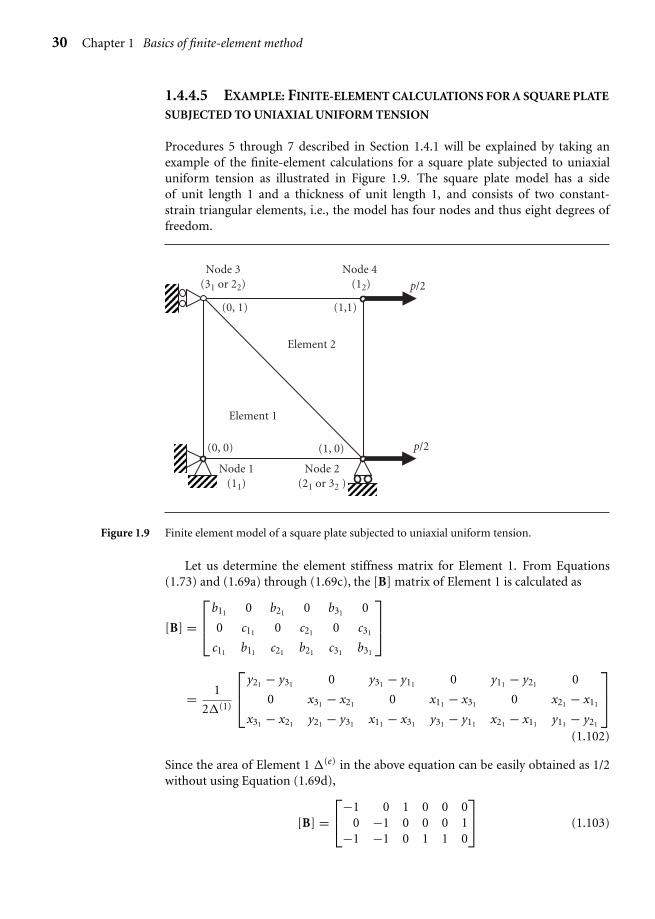
Ch01-H6875.tex 24/11/2006 17: 0 page 30


1.4.4.5 EXAMPLE: FINITE-ELEMENT CALCULATIONS FOR A SQUARE PLATE

SUBJECTED TO UNIAXIAL UNIFORM TENSION

Procedures 5 through 7 described in Section 1.4.1 will be explained by taking anexample of the finite-element calculations for a square plate subjected to uniaxialuniform tension as illustrated in Figure 1.9. The square plate model has a sideof unit length 1 and a thickness of unit length 1, and consists of two constant-strain triangular elements, i.e., the model has four nodes and thus eight degrees offreedom.

Node 3(31 or 22)

Node 4 (12)

Node 1(11)

Node 2(21 or 32 )

Element 1

Element 2

(0, 1)

(0, 0) (1, 0) p/2

p/2

(1,1)

Figure 1.9 Finite element model of a square plate subjected to uniaxial uniform tension.

Let us determine the element stiffness matrix for Element 1. From Equations(1.73) and (1.69a) through (1.69c), the [B] matrix of Element 1 is calculated as

[B] =⎡⎢⎣

b11 0 b21 0 b31 0

0 c11 0 c21 0 c31

c11 b11 c21 b21 c31 b31

⎤⎥⎦

= 1

2�(1)

⎡⎢⎣

y21 − y31 0 y31 − y11 0 y11 − y21 0

0 x31 − x21 0 x11 − x31 0 x21 − x11

x31 − x21 y21 − y31 x11 − x31 y31 − y11 x21 − x11 y11 − y21

⎤⎥⎦

(1.102)

Since the area of Element 1 �(e) in the above equation can be easily obtained as 1/2without using Equation (1.69d),

[B] =⎡⎣−1 0 1 0 0 0

0 −1 0 0 0 1−1 −1 0 1 1 0

⎤⎦ (1.103)

Ch01-H6875.tex 24/11/2006 17: 0 page 31


Hence, from Equation (1.85), the element stiffness matrix for Element 1 [k(e)] iscalculated as

[k(1)] = t

2

E′

1 − ν′2

⎡⎢⎢⎢⎢⎢⎢⎣

−1 0 −10 −1 −11 0 00 0 10 0 10 1 0

⎤⎥⎥⎥⎥⎥⎥⎦⎡⎣1 ν′ 0

ν′ 1 00 0 α

⎤⎦⎡⎣−1 0 1 0 0 0

0 −1 0 0 0 1−1 −1 0 1 1 0

⎤⎦

(1.104)

where α = (1 − ν′)/2. After multiplication of the matrices in Equation (1.104), theelement stiffness equation is obtained from Equation (1.84) as

⎧⎪⎪⎪⎪⎪⎪⎪⎪⎪⎪⎪⎨⎪⎪⎪⎪⎪⎪⎪⎪⎪⎪⎪⎩

X(1)11

Y (1)11

X(1)21

Y (1)21

X(1)31

Y (1)31

⎫⎪⎪⎪⎪⎪⎪⎪⎪⎪⎪⎪⎬⎪⎪⎪⎪⎪⎪⎪⎪⎪⎪⎪⎭

= t

2

E′

1 − ν′2

⎡⎢⎢⎢⎢⎢⎢⎢⎢⎢⎢⎢⎣

1 + α ν′ + α −1 −α −α −ν′

ν′ + α 1 + α −ν′ −α −α −1

−1 −ν′ 1 0 0 ν′

−α −α 0 α α 0

−α −α 0 α α 0

−ν′ −1 ν′ 0 0 1

⎤⎥⎥⎥⎥⎥⎥⎥⎥⎥⎥⎥⎦

⎧⎪⎪⎪⎪⎪⎪⎪⎪⎪⎪⎪⎨⎪⎪⎪⎪⎪⎪⎪⎪⎪⎪⎪⎩

u11

v11

u21

v21

u31

v31

⎫⎪⎪⎪⎪⎪⎪⎪⎪⎪⎪⎪⎬⎪⎪⎪⎪⎪⎪⎪⎪⎪⎪⎪⎭

(1.105)

since the equivalent nodal forces due to initial strains ε0 and body forces Fx and Fy ,{Fε0}(1) and {FF}(1) are zero. The components of the nodal displacement and forcevectors are written by the element nodal numbers. By rewriting these components bythe global nodal numbers as shown in Figure 1.9, Equation (1.105) is rewritten as

⎧⎪⎪⎪⎪⎪⎪⎪⎪⎨⎪⎪⎪⎪⎪⎪⎪⎪⎩

X1

Y1

X2

Y2

X3

Y3

⎫⎪⎪⎪⎪⎪⎪⎪⎪⎬⎪⎪⎪⎪⎪⎪⎪⎪⎭

= t

2

E′

1 − ν′2

⎡⎢⎢⎢⎢⎢⎢⎢⎢⎢⎣

1 + α ν′ + α −1 −α −α −ν′

ν′ + α 1 + α −ν′ −α −α −1

−1 −ν′ 1 0 0 ν′

−α −α 0 α α 0

−α −α 0 α α 0

−ν′ −1 ν′ 0 0 1

⎤⎥⎥⎥⎥⎥⎥⎥⎥⎥⎦

⎧⎪⎪⎪⎪⎪⎪⎪⎪⎨⎪⎪⎪⎪⎪⎪⎪⎪⎩

u1

v1

u2

v2

u3

v3

⎫⎪⎪⎪⎪⎪⎪⎪⎪⎬⎪⎪⎪⎪⎪⎪⎪⎪⎭

(1.106)

In a similar way, the element stiffness equation for Element 2 is obtained as

⎧⎪⎪⎪⎪⎪⎪⎪⎪⎪⎪⎪⎨⎪⎪⎪⎪⎪⎪⎪⎪⎪⎪⎪⎩

X(2)12

Y (2)12

X(2)22

Y (2)22

X(2)32

Y (2)32

⎫⎪⎪⎪⎪⎪⎪⎪⎪⎪⎪⎪⎬⎪⎪⎪⎪⎪⎪⎪⎪⎪⎪⎪⎭

= t

2

E′

1 − ν′2

⎡⎢⎢⎢⎢⎢⎢⎣

1 + α ν′ + α −1 −α −α −ν′ν′ + α 1 + α −ν′ −α −α −1−1 −ν′ 1 0 0 ν′−α −α 0 α α 0−α −α 0 α α 0−ν′ −1 ν′ 0 0 1

⎤⎥⎥⎥⎥⎥⎥⎦

⎧⎪⎪⎪⎪⎪⎪⎨⎪⎪⎪⎪⎪⎪⎩

u12

v12

u22

v22

u32

v32

⎫⎪⎪⎪⎪⎪⎪⎬⎪⎪⎪⎪⎪⎪⎭

(1.107)

Ch01-H6875.tex 24/11/2006 17: 0 page 32


and is rewritten by using the global nodal numbers as

⎧⎪⎪⎪⎪⎪⎪⎪⎪⎨⎪⎪⎪⎪⎪⎪⎪⎪⎩

X4

Y4

X3

Y3

X2

Y2

⎫⎪⎪⎪⎪⎪⎪⎪⎪⎬⎪⎪⎪⎪⎪⎪⎪⎪⎭

= t

2

E′

1 − ν′2

⎡⎢⎢⎢⎢⎢⎢⎢⎢⎣

1 + α ν′ + α −1 −α −α −ν′

ν′ + α 1 + α −ν′ −α −α −1

−1 −ν′ 1 0 0 ν′

−α −α 0 α α 0

−α −α 0 α α 0

−ν′ −1 ν′ 0 0 1

⎤⎥⎥⎥⎥⎥⎥⎥⎥⎦

⎧⎪⎪⎪⎪⎪⎪⎪⎪⎨⎪⎪⎪⎪⎪⎪⎪⎪⎩

u4

v4

u3

v3

u2

v2

⎫⎪⎪⎪⎪⎪⎪⎪⎪⎬⎪⎪⎪⎪⎪⎪⎪⎪⎭

(1.108)

By assembling the two-element stiffness matrices, the following global stiffnessequation for the square plate subjected to uniform tension is obtained (Procedure 4):

t

2

E′

1 − ν′2

⎡⎢⎢⎢⎢⎢⎢⎢⎢⎢⎢⎢⎢⎢⎣

1 + α ν′ + α −1 −α −α −ν′ 0 0

ν′ + α 1 + α −ν′ −α −α −1 0 0

−1 −ν′ 1 + α 0 0 ν′ + α −α −α

−α −α 0 1 + α ν′ + α 0 −ν′ −1

−α −α 0 ν′ + α 1 + α 0 −1 −ν′

−ν′ −1 ν′ + α 0 0 1 + α −α −α

0 0 −α −ν′ −1 −α 1 + α ν′ + α

0 0 −α −1 −ν′ −α ν′ + α 1 + α

⎤⎥⎥⎥⎥⎥⎥⎥⎥⎥⎥⎥⎥⎥⎦

×

⎧⎪⎪⎪⎪⎪⎪⎪⎪⎪⎪⎪⎪⎪⎨⎪⎪⎪⎪⎪⎪⎪⎪⎪⎪⎪⎪⎪⎩

u1

v1

u2

v2

u3

v3

u4

v4

⎫⎪⎪⎪⎪⎪⎪⎪⎪⎪⎪⎪⎪⎪⎬⎪⎪⎪⎪⎪⎪⎪⎪⎪⎪⎪⎪⎪⎭

=

⎧⎪⎪⎪⎪⎪⎪⎪⎪⎪⎪⎪⎪⎪⎨⎪⎪⎪⎪⎪⎪⎪⎪⎪⎪⎪⎪⎪⎩

X1

Y1

X2

Y2

X3

Y3

X4

Y4

⎫⎪⎪⎪⎪⎪⎪⎪⎪⎪⎪⎪⎪⎪⎬⎪⎪⎪⎪⎪⎪⎪⎪⎪⎪⎪⎪⎪⎭

(1.109)

where the left- and right-hand sides of the equation are replaced with each other.Let us now impose boundary conditions on the nodes. Namely, the node 1 is

clamped in both the x- and the y-directions, the node 2 is clamped only in the x-direction, and the nodes 2 and 4 are subjected to equal nodal forces X2 = X4 = (p ×1 × 1)/2 = p/2, respectively, in the x-direction. A pair of the equal nodal forcesp/2 applied to the nodes 2 and 4 in the x-direction is the finite-element model ofa uniformly distributed tension force p per unit area exerted on the side 24 in thex-direction as illustrated in Figure 1.9. The geometrical boundary and mechanicalconditions for the present case are

u1 = v1 = v2 = u3 = 0 (1.110)

and

X2 = X4 = (pt)/2 = p/2 Y3 = Y4 = 0 (1.111)

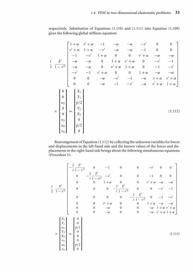
Ch01-H6875.tex 24/11/2006 17: 0 page 33


respectively. Substitution of Equations (1.110) and (1.111) into Equation (1.109)gives the following global stiffness equation:

t

2

E′

1 − ν′2

⎡⎢⎢⎢⎢⎢⎢⎢⎢⎢⎢⎢⎢⎢⎣

1 + α ν′ + α −1 −α −α −ν′ 0 0

ν′ + α 1 + α −ν′ −α −α −1 0 0

−1 −ν′ 1 + α 0 0 ν′ + α −α −α

−α −α 0 1 + α ν′ + α 0 −ν′ −1

−α −α 0 ν′ + α 1 + α 0 −1 −ν′

−ν′ −1 ν′ + α 0 0 1 + α −α −α

0 0 −α −ν′ −1 −α 1 + α ν′ + α

0 0 −α −1 −ν′ −α ν′ + α 1 + α

⎤⎥⎥⎥⎥⎥⎥⎥⎥⎥⎥⎥⎥⎥⎦

×

⎧⎪⎪⎪⎪⎪⎪⎪⎪⎪⎪⎪⎪⎪⎨⎪⎪⎪⎪⎪⎪⎪⎪⎪⎪⎪⎪⎪⎩

0

0

u2

0

0

v3

u4

v4

⎫⎪⎪⎪⎪⎪⎪⎪⎪⎪⎪⎪⎪⎪⎬⎪⎪⎪⎪⎪⎪⎪⎪⎪⎪⎪⎪⎪⎭

=

⎧⎪⎪⎪⎪⎪⎪⎪⎪⎪⎪⎪⎪⎪⎨⎪⎪⎪⎪⎪⎪⎪⎪⎪⎪⎪⎪⎪⎩

X1

Y1

p/2

Y2

X3

0

p/2

0

⎫⎪⎪⎪⎪⎪⎪⎪⎪⎪⎪⎪⎪⎪⎬⎪⎪⎪⎪⎪⎪⎪⎪⎪⎪⎪⎪⎪⎭

(1.112)

Rearrangement of Equation (1.112) by collecting the unknown variables for forcesand displacements in the left-hand side and the known values of the forces and dis-placements in the right-hand side brings about the following simultaneous equations(Procedure 5):

t

2

E′

1 − ν′2

⎡⎢⎢⎢⎢⎢⎢⎢⎢⎢⎢⎢⎢⎢⎢⎢⎢⎢⎢⎣

−2

t

E′

1 − ν′2 0 −1 0 0 −ν′ 0 0

0 −2

t

E′

1 − ν′2 −ν′ 0 0 −1 0 0

0 0 1 + α 0 0 ν′ + α −α −α

0 0 0 −2

t

E′

1 − ν′2 0 0 −ν′ −1

0 0 0 0 −2

t

E′

1 − ν′2 0 −1 −ν′

0 0 ν′ + α 0 0 1 + α −α −α

0 0 −α 0 0 −α 1 + α ν′ + α

0 0 −α 0 0 −α ν′ + α 1 + α

⎤⎥⎥⎥⎥⎥⎥⎥⎥⎥⎥⎥⎥⎥⎥⎥⎥⎥⎥⎦

×

⎧⎪⎪⎪⎪⎪⎪⎪⎪⎪⎪⎨⎪⎪⎪⎪⎪⎪⎪⎪⎪⎪⎩

X1

Y1

u2

Y2

X3

v3

u4

v4

⎫⎪⎪⎪⎪⎪⎪⎪⎪⎪⎪⎬⎪⎪⎪⎪⎪⎪⎪⎪⎪⎪⎭

=

⎧⎪⎪⎪⎪⎪⎪⎪⎪⎪⎪⎨⎪⎪⎪⎪⎪⎪⎪⎪⎪⎪⎩

00

p/2000

p/20

⎫⎪⎪⎪⎪⎪⎪⎪⎪⎪⎪⎬⎪⎪⎪⎪⎪⎪⎪⎪⎪⎪⎭

(1.113)

Ch01-H6875.tex 24/11/2006 17: 0 page 34


Equation (1.113) can be solved numerically by, for instance, the Gauss eliminationprocedure. The solutions for Equation (1.113) are

u2 = u4 = p/E′, v3 = v4 = −ν′p/E′, X1 = X3 = −p/2, Y1 = Y2 = 0 (1.114)

(Procedure 6).The strains and stresses in the square plate can be calculated by substituting the

solutions (1.114) into Equations (1.73) and (1.74), respectively (Procedure 7). Theresultant strains and stresses are given by the following equations:

⎧⎨⎩

εx

εy

γxy

⎫⎬⎭ = [B]

⎧⎪⎪⎪⎪⎪⎪⎨⎪⎪⎪⎪⎪⎪⎩

u4

v4

u3

v3

u2

v2

⎫⎪⎪⎪⎪⎪⎪⎬⎪⎪⎪⎪⎪⎪⎭

= p

E′

⎡⎣1 0 −1 0 0 0

0 1 0 0 0 −11 1 0 1 −1 0

⎤⎦⎧⎪⎪⎪⎪⎪⎪⎨⎪⎪⎪⎪⎪⎪⎩

1−ν′

0ν′10

⎫⎪⎪⎪⎪⎪⎪⎬⎪⎪⎪⎪⎪⎪⎭

= p

E′

⎧⎨⎩

1−ν′

1 − ν′ + ν′ − 1

⎫⎬⎭ = p

E′

⎧⎨⎩

1−ν′

0

⎫⎬⎭ (1.115)

and

⎧⎨⎩

σx

σy

τxy

⎫⎬⎭ = E′

1 − ν′2

⎡⎢⎣

1 ν′ 0ν′ 1 0

0 01 − ν′

2

⎤⎥⎦⎧⎪⎨⎪⎩

εx

εy

γxy

⎫⎪⎬⎪⎭ = p

1 − ν′2

⎡⎢⎣

1 ν′ 0ν′ 1 0

0 01 − ν′

2

⎤⎥⎦⎧⎪⎨⎪⎩

1

−ν′

0

⎫⎪⎬⎪⎭

= p

1 − ν′2

⎧⎨⎩

1 − ν′200

⎫⎬⎭ = p

⎧⎨⎩

100

⎫⎬⎭ (1.116)

The results obtained by the present finite-element calculations imply that a squareplate subjected to uniaxial uniform tension in the x-direction is elongated by a uni-form strain of p/E′ in the loading direction, whereas it is contacted by a uniform strainof −ν′p/E′ in the direction perpendicular to the loading direction and that only a uni-form normal stress of σx = p is induced in the plate. The result that the nodal reactionforces at the nodes 1 and 3 are equal to −p/2, i.e., X1 = X3 = −p/2 implies that a uni-form reaction force of −p is produced along the side 13. It is concluded that the aboveresults obtained by the FEM agree well with the physical interpretations of the presentproblem.

Bibliography

1. O. C. Zienkiewicz and K. Morgan, Finite Elements and Approximation, John Wiley &Sons, New York (1983).

2. O. C. Zienkiewicz and R. Taylor, The Finite Element Method (4th edn), Vol. 1,McGraw-Hill, London (1989).

Ch01-H6875.tex 24/11/2006 17: 0 page 35

Bibliography 35

3. G. W. Rowe et al., Finite-Element Plasticity and Metalforming Analysis, CambridgeUniversity Press, (1991).

4. C. L. Dym and I. H. Shames, Solid Mechanics: A Variational Approach, McGraw-Hill, New York (1973).

5. K. Washizu, Variational Methods in Elasticity and Plasticity (2nd edn), Pergamon,New York (1975).

6. K.-J. Bathe, Finite Element Procedures, Printice-Hall Int., New Jersy (1975).

7. B. A. Finlayson, The Method of Weighted Residuals and Variational Principles,Academic Press, New York (1972).

8. M. Gotoh, Engineering Finite Element Method – For Analysis of Large Elastic–PlasticDeformation, Corona Publishing Co., Ltd., Tokyo (1995) (in Japanese).

9. H. Togawa, Introduction to the Finite Element Method, Baifukan Co., Ltd., Tokyo(1984) (in Japanese).

10. G. Yagawa et al., Computational Mechanics, Iwanami Shoten Publishers, Tokyo(2000) (in Japanese).

11. K. Washizu et al., Handbook of the Finite Element Method (Basics), Baifukan Co.,Ltd., Tokyo (1994) (in Japanese).

Ch02-H6875.tex 24/11/2006 17: 2 page 37

2C h a p t e r

Overview ofANSYS structure

and visualcapabilities

Chapter outline

2.1 Introduction 372.2 Starting the program 382.3 Preprocessing stage 432.4 Solution stage 492.5 Postprocessing stage 50

2.1 Introduction

ANSYS is a general-purpose finite-element modeling package for numericallysolving a wide variety of mechanical problems. These problems include static/

dynamic, structural analysis (both linear and nonlinear), heat transfer, and fluidproblems, as well as acoustic and electromagnetic problems.

In general, a finite-element solution may be broken into the following three stages.

(1) Preprocessing: defining the problemThe major steps in preprocessing are (i) define keypoints/lines/areas/volumes,(ii) define element type and material/geometric properties, and (iii) meshlines/areas/ volumes as required.

37

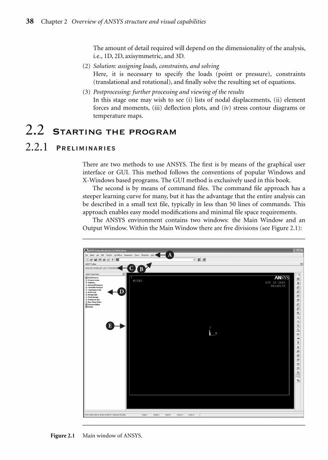
Ch02-H6875.tex 24/11/2006 17: 2 page 38

38 Chapter 2 Overview of ANSYS structure and visual capabilities

The amount of detail required will depend on the dimensionality of the analysis,i.e., 1D, 2D, axisymmetric, and 3D.

(2) Solution: assigning loads, constraints, and solvingHere, it is necessary to specify the loads (point or pressure), constraints(translational and rotational), and finally solve the resulting set of equations.

(3) Postprocessing: further processing and viewing of the resultsIn this stage one may wish to see (i) lists of nodal displacements, (ii) elementforces and moments, (iii) deflection plots, and (iv) stress contour diagrams ortemperature maps.

2.2 Starting the program

2.2.1 Preliminaries

There are two methods to use ANSYS. The first is by means of the graphical userinterface or GUI. This method follows the conventions of popular Windows andX-Windows based programs. The GUI method is exclusively used in this book.

The second is by means of command files. The command file approach has asteeper learning curve for many, but it has the advantage that the entire analysis canbe described in a small text file, typically in less than 50 lines of commands. Thisapproach enables easy model modifications and minimal file space requirements.

The ANSYS environment contains two windows: the Main Window and anOutput Window. Within the Main Window there are five divisions (see Figure 2.1):

D

C B

A

E

Figure 2.1 Main window of ANSYS.

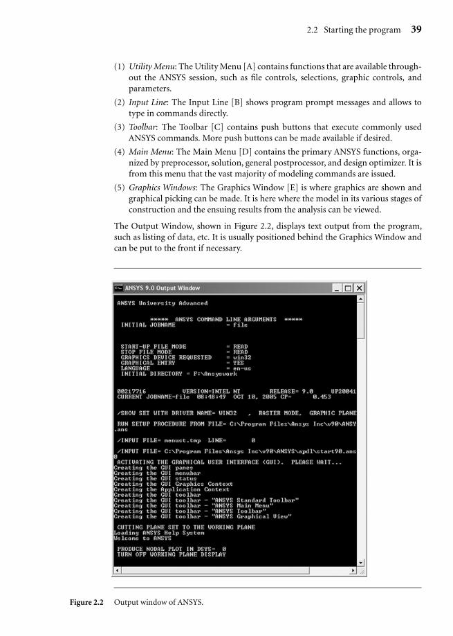
Ch02-H6875.tex 24/11/2006 17: 2 page 39

2.2 Starting the program 39

(1) Utility Menu: The Utility Menu [A] contains functions that are available through-out the ANSYS session, such as file controls, selections, graphic controls, andparameters.

(2) Input Line: The Input Line [B] shows program prompt messages and allows totype in commands directly.

(3) Toolbar: The Toolbar [C] contains push buttons that execute commonly usedANSYS commands. More push buttons can be made available if desired.

(4) Main Menu: The Main Menu [D] contains the primary ANSYS functions, orga-nized by preprocessor, solution, general postprocessor, and design optimizer. It isfrom this menu that the vast majority of modeling commands are issued.

(5) Graphics Windows: The Graphics Window [E] is where graphics are shown andgraphical picking can be made. It is here where the model in its various stages ofconstruction and the ensuing results from the analysis can be viewed.

The Output Window, shown in Figure 2.2, displays text output from the program,such as listing of data, etc. It is usually positioned behind the Graphics Window andcan be put to the front if necessary.

Figure 2.2 Output window of ANSYS.

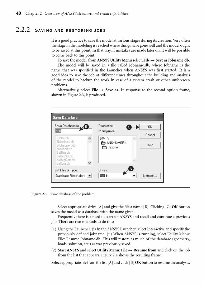
Ch02-H6875.tex 24/11/2006 17: 2 page 40


2.2.2 Saving and restoring jobs

It is a good practice to save the model at various stages during its creation. Very oftenthe stage in the modeling is reached where things have gone well and the model oughtto be saved at this point. In that way, if mistakes are made later on, it will be possibleto come back to this point.

To save the model, from ANSYS Utility Menu select, File → Save as Jobname.db.The model will be saved in a file called Jobname.db, where Jobname is the

name that was specified in the Launcher when ANSYS was first started. It is agood idea to save the job at different times throughout the building and analysisof the model to backup the work in case of a system crash or other unforeseenproblems.

Alternatively, select File → Save as. In response to the second option frame,shown in Figure 2.3, is produced.

B C

A

Figure 2.3 Save database of the problem.

Select appropriate drive [A] and give the file a name [B]. Clicking [C] OK buttonsaves the model as a database with the name given.

Frequently there is a need to start up ANSYS and recall and continue a previousjob. There are two methods to do this:

(1) Using the Launcher. (i) In the ANSYS Launcher, select Interactive and specify thepreviously defined jobname. (ii) When ANSYS is running, select Utility Menu:File: Resume Jobname.db. This will restore as much of the database (geometry,loads, solution, etc.) as was previously saved.

(2) Start ANSYS and select Utility Menu: File → Resume from and click on the jobfrom the list that appears. Figure 2.4 shows the resulting frame.

Select appropriate file from the list [A] and click [B] OK button to resume the analysis.

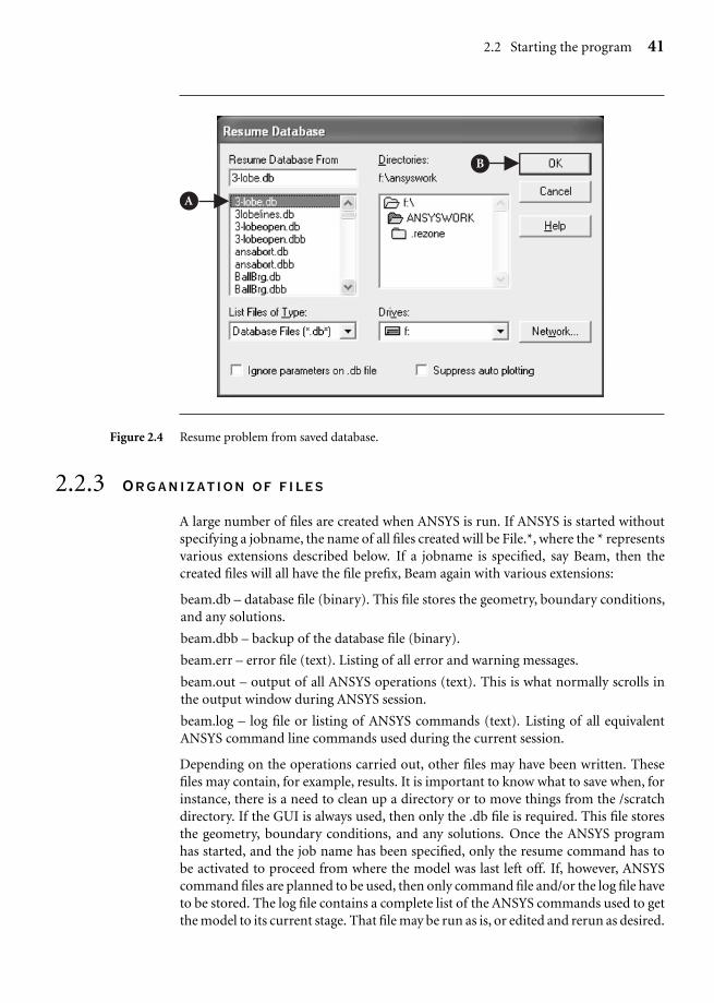
Ch02-H6875.tex 24/11/2006 17: 2 page 41

2.2 Starting the program 41

A

B

Figure 2.4 Resume problem from saved database.

2.2.3 Organization of files

A large number of files are created when ANSYS is run. If ANSYS is started withoutspecifying a jobname, the name of all files created will be File.*, where the * representsvarious extensions described below. If a jobname is specified, say Beam, then thecreated files will all have the file prefix, Beam again with various extensions:

beam.db – database file (binary). This file stores the geometry, boundary conditions,and any solutions.

beam.dbb – backup of the database file (binary).

beam.err – error file (text). Listing of all error and warning messages.

beam.out – output of all ANSYS operations (text). This is what normally scrolls inthe output window during ANSYS session.

beam.log – log file or listing of ANSYS commands (text). Listing of all equivalentANSYS command line commands used during the current session.

Depending on the operations carried out, other files may have been written. Thesefiles may contain, for example, results. It is important to know what to save when, forinstance, there is a need to clean up a directory or to move things from the /scratchdirectory. If the GUI is always used, then only the .db file is required. This file storesthe geometry, boundary conditions, and any solutions. Once the ANSYS programhas started, and the job name has been specified, only the resume command has tobe activated to proceed from where the model was last left off. If, however, ANSYScommand files are planned to be used, then only command file and/or the log file haveto be stored. The log file contains a complete list of the ANSYS commands used to getthe model to its current stage. That file may be run as is, or edited and rerun as desired.

Ch02-H6875.tex 24/11/2006 17: 2 page 42


2.2.4 Printing and plotting

ANSYS produces lists and tables of many types of results that are normally displayedon the screen. However, it is often desired to save the results to a file to be lateranalyzed or included in a report.

In case of stresses, instead of using Plot Results to plot the stresses, choose ListResults. In the same way as described above. When the list appears on the screen inits own window, select File: Save As and give a file name to store the results. Any othersolution can be done in the same way. For example, select Nodal Solution from theList Results menu to get displacements. Preprocessing and Solution data can be listedand saved from the List Menu in the ANSYS Utility Menu. Save the resulting list inthe same way described above.

When there is a need to quickly save an image of the entire screen or the currentGraphics Window, from ANSYS Utility Menu select Plot Ctrls → Hard Copy. Thereare two options, namely To Printer (see Figure 2.5) and To File (see Figure 2.6).

In the frame shown in Figure 2.5, select the printer [A] from the list of printersand press [B] Print button.

A

B

Figure 2.5 Print to printer.

A

B

C

D

E

Figure 2.6 Print to file.

Ch02-H6875.tex 24/11/2006 17: 2 page 43

2.3 Preprocessing stage 43

In the frame that is shown in Figure 2.6, an example selection could be [A] Color,[B] BMP, [C] Reverse Video, and finally [D] Save to. Then enter an appropriate filename and click [E] OK button. This image file may now be printed on a PostScriptprinter or included in a document.

2.2.5 Exiting the program

The ANSYS program can be exited in a number of different ways. When the currentanalysis is saved from Utility Menu select File → Exit. A frame shown in Figure 2.7appears.

A

Figure 2.7 Exit from ANSYS.

There are four options, depending on what is important to be saved. If nothing isto be saved then select [A] Quite – No Save as indicated.

2.3 Preprocessing stage

2.3.1 Building a model

The ANSYS program has many finite-element analysis capabilities, ranging froma simple linear static analysis to a complex nonlinear transient dynamic analysis.Building a finite-element model requires more time than any other part of the analysis.First, a jobname and analysis title have to be specified. Next, the PREP7 preprocessor isused to define the element types, element real constants, material properties, and themodel geometry. It is important to remember that ANSYS does not assume a systemof units for intended analysis. Except in magnetic field analyses, any system of unitscan be used so long as it is ensured that units are consistent for all input data. Units

Ch02-H6875.tex 24/11/2006 17: 2 page 44


cannot be set directly from the GUI. In order to set units as the international systemof units (SI) from ANSYS Main Menu, select Preprocessor → Material Props →Material Library → Select Units. Figure 2.8 shows the resulting frame.

A

Figure 2.8 Selection of units for the problem.

Activate [A] SI (MKS) button to inform the ANSYS program that this system ofunits is proposed to be used in the analysis.

2.3.1.1 Defining element types and real constants

The ANSYS element library contains more than 100 different element types. Eachelement type has a unique number and a prefix that identifies the element category.In order to define element types, one must be in PREP7. From ANSYS Main Menu,select Preprocessor or → Element Type → Add/Edit/Delete. In response, the frameshown in Figure 2.9 appears.

Click on [A] Add button and a new frame, shown in Figure 2.10, appears.Select an appropriate element type for the analysis performed, e.g., [A] Solid and

[B] 8node 183 as shown in Figure 2.10.Element real constants are properties that depend on the element type, such

as cross-sectional properties of a beam element. As with element types, each setof real constant has a reference number and the table of reference number versusreal constant set is called the real constant table. Not all element types require realconstant, and different elements of the same type may have different real constantvalues. ANSYS Main Menu command Preprocessor → Modeling → Create →

Ch02-H6875.tex 24/11/2006 17: 2 page 45


A

Figure 2.9 Definition of element types to be used.

A

B

Figure 2.10 Selection of element types from the library.

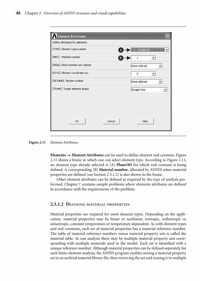
Ch02-H6875.tex 24/11/2006 17: 2 page 46


A

B

Figure 2.11 Element Attributes.

Elements → Element Attributes can be used to define element real constant. Figure2.11 shows a frame in which one can select element type. According to Figure 2.11,an element type already selected is [A] Plane183 for which real constant is beingdefined. A corresponding [B] Material number, allocated by ANSYS when materialproperties are defined (see Section 2.3.1.2) is also shown in the frame.

Other element attributes can be defined as required by the type of analysis per-formed. Chapter 7 contains sample problems where elements attributes are definedin accordance with the requirements of the problem.

2.3.1.2 Defining material properties

Material properties are required for most element types. Depending on the appli-cation, material properties may be linear or nonlinear, isotropic, orthotropic oranisotropic, constant temperature or temperature dependent. As with element typesand real constants, each set of material properties has a material reference number.The table of material reference numbers versus material property sets is called thematerial table. In one analysis there may be multiple material property sets corre-sponding with multiple materials used in the model. Each set is identified with aunique reference number. Although material properties can be defined separately foreach finite-element analysis, the ANSYS program enables storing a material propertyset in an archival material library file, then retrieving the set and reusing it in multiple

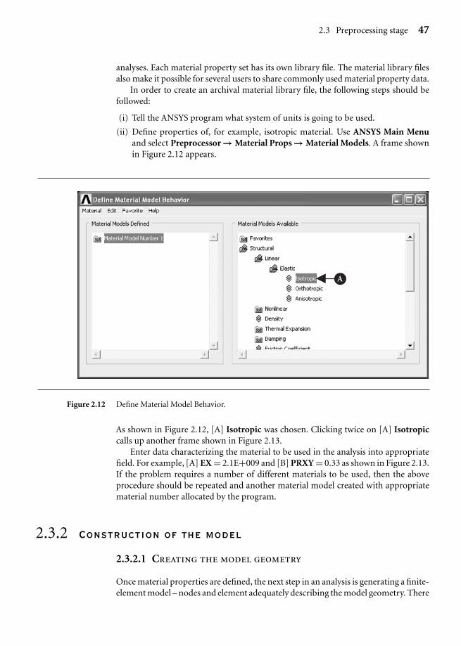
Ch02-H6875.tex 24/11/2006 17: 2 page 47


analyses. Each material property set has its own library file. The material library filesalso make it possible for several users to share commonly used material property data.

In order to create an archival material library file, the following steps should befollowed:

(i) Tell the ANSYS program what system of units is going to be used.

(ii) Define properties of, for example, isotropic material. Use ANSYS Main Menuand select Preprocessor → Material Props → Material Models. A frame shownin Figure 2.12 appears.

A

Figure 2.12 Define Material Model Behavior.

As shown in Figure 2.12, [A] Isotropic was chosen. Clicking twice on [A] Isotropiccalls up another frame shown in Figure 2.13.

Enter data characterizing the material to be used in the analysis into appropriatefield. For example, [A] EX = 2.1E+009 and [B] PRXY = 0.33 as shown in Figure 2.13.If the problem requires a number of different materials to be used, then the aboveprocedure should be repeated and another material model created with appropriatematerial number allocated by the program.

2.3.2 Construction of the model

2.3.2.1 Creating the model geometry

Once material properties are defined, the next step in an analysis is generating a finite-element model – nodes and element adequately describing the model geometry. There

Ch02-H6875.tex 24/11/2006 17: 2 page 48


A

B

Figure 2.13 Linear isotropic material properties.

are two methods to create the finite-element model: solid modeling and direct gener-ation. With solid modeling, the geometry of shape of the model is described, and thenthe ANSYS program automatically meshes the geometry with nodes and elements.The size and shape of the elements that the program creates can be controlled. Withdirect generation, the location of each node and the connectivity of each elementis manually defined. Several convenience operations, such as copying patterns ofexisting nodes and elements, symmetry reflection, etc., are available.

Solved example problems in this book amply illustrate, in a step-by-step manner,how to create the model geometry.

2.3.2.2 Applying loads

Loads can be applied using either PREP7 preprocessor or the SOLUTION processor.Regardless of the chosen strategy, it is necessary to define the analysis type and analysisoptions, apply loads, specify load step options, and initiate the finite-element solution.

The analysis type to be used is based on the loading conditions and the responsewhich is wished to calculate. For example, if natural frequencies and mode shapesare to be calculated, then a modal analysis ought to be chosen. The ANSYS pro-gram offers the following analysis types: static (or steady-state), transient, harmonic,modal, spectrum, buckling, and substructuring. Not all analysis types are valid forall disciplines. Modal analysis, for instance, is not valid for thermal models. Analy-sis options allow for customization of analysis type. Typical analysis options are themethod of solution, stress stiffening on or off, and Newton–Raphson options. Inorder to define the analysis type and analysis options, use ANSYS Main Menu andselect Main Menu: Preprocessor → Loads → Analysis Type → New Analysis. Inresponse to the selection, the frame shown in Figure 2.14 appears.

Ch02-H6875.tex 24/11/2006 17: 2 page 49

2.4 Solution stage 49

A

Figure 2.14 Type of analysis definition.

Select the type of analysis that is appropriate for the problem at hand byactivating [A] Static button for example.

The word loads used here includes boundary conditions, i.e., constraints, sup-ports, or boundary field specifications. It also includes other externally and internallyapplied loads. Loads in the ANSYS program are divided into six categories: DOFconstraints, forces, surface loads, body loads, inertia loads, and coupled field loads.Most of these loads can be applied either on the solid model (keypoints, lines, andareas) or the finite-element model (nodes and elements).

There are two important load-related terms. A load step is simply a configurationof loads for which the solution is obtained. In a structural analysis, for instance, windloads may be applied in one load step and gravity in a second load step. Load stepsare also useful in dividing a transient load history curve into several segments.

Substeps are incremental steps taken within a load step. They are mainly used foraccuracy and convergence purposes in transient and nonlinear analyses. Substeps arealso known as time steps which are taken over a period of time.

Load step options are alternatives that can be changed from load step to loadstep, such as number of substeps, time at the end of a load step, and output controls.Depending on the type of analysis performed, load step options may or may not berequired. Sample problems solved here provide practical guide to appropriate loadstep options as necessary.

2.4 Solution stage

To initiate solution calculations, use ANSYS Main Menu selecting Solution →Solve → Current LS. Figure 2.15 shows resulting frame.

Ch02-H6875.tex 24/11/2006 17: 2 page 50


A

Figure 2.15 Start solution of current problem.

After reviewing the summary information about the model, click [A] OK buttonto start the solution. When this command is issued, the ANSYS program takes modeland loading information from the database and calculates the results. Results arewritten to the results file and also to the database. The only difference is that only oneset of results can reside in the database at one time, while a number of result sets canbe written to the results file.

Once the solution has been calculated, the ANSYS postprocessors can be used toreview the results.

2.5 Postprocessing stage

Two postprocessors are available:

(1) POST1: The general postprocessor is used to review results at one substep (timestep) over the entire model or selected portion of the model. The command toenter POST1 requires selection from ANSYS Main Menu General Postprocessor.Using this postprocessor contour displays, deformed shapes, and tabular listingsto review and interpret the results of the analysis can be obtained. POST1 offersmany other capabilities, including error estimation, load case combinations,calculations among results data, and path operations.

(2) POST26: The time history postprocessor is used to review results at specific pointsin the model over all time steps. The command to enter POST26 is as follows: fromANSYS Main Menu select TimeHist Postprocessor. Graph plots of results dataversus time (or frequency) and tabular listings can be obtained. Other POST26capabilities include arithmetic calculations and complex algebra.

Ch03-H6875.tex 24/11/2006 17: 2 page 51

3C h a p t e r

Application ofANSYS to Stress

Analysis

Chapter outline

3.1 Cantilever beam 513.2 The principle of St. Venant 843.3 Stress concentration due to elliptic holes 933.4 Stress singularity problem 1063.5 Two-dimensional contact stress 120References 141

3.1 Cantilever beam

Beams are important fundamental structural and/or machine elements; theyare found in buildings and in bridges. Beams are also used as shafts in cars

and trains, as wings in aircrafts and bookshelves in bookstores. Arms and femurs ofhuman beings and branches of trees are good examples of portions of living creatureswhich support their bodies. Beams play important roles not only in inorganic butalso in organic structures.

Mechanics of beams is one of the most important subjects in engineering.

51

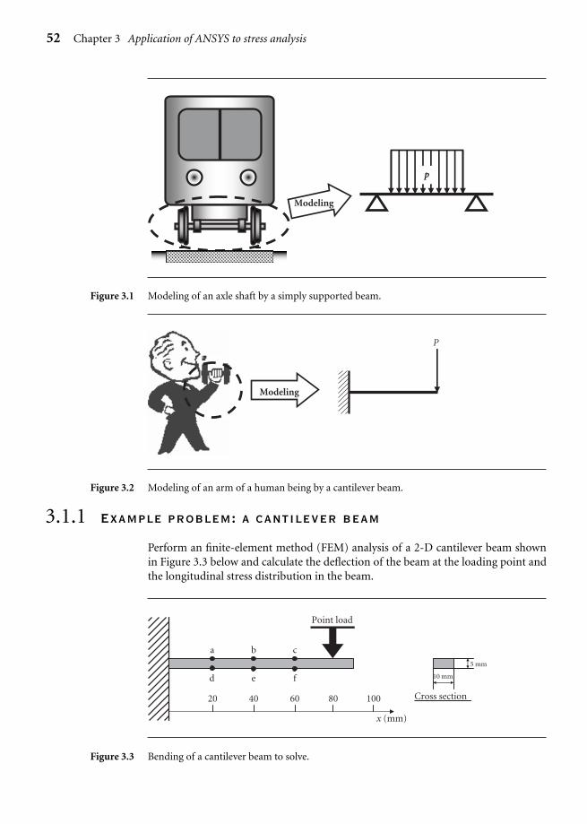
Ch03-H6875.tex 24/11/2006 17: 2 page 52

52 Chapter 3 Application of ANSYS to stress analysis

Modeling

p

Figure 3.1 Modeling of an axle shaft by a simply supported beam.

Modeling

P

Figure 3.2 Modeling of an arm of a human being by a cantilever beam.

3.1.1 Example problem: a cantilever beam

Perform an finite-element method (FEM) analysis of a 2-D cantilever beam shownin Figure 3.3 below and calculate the deflection of the beam at the loading point andthe longitudinal stress distribution in the beam.

a b

d e

x (mm)

20 40 60 80 Cross section

10 mm

5 mm

100

Point load

c

f

Figure 3.3 Bending of a cantilever beam to solve.

Ch03-H6875.tex 24/11/2006 17: 2 page 53

3.1 Cantilever beam 53

3.1.2 Problem description

Geometry: length l = 90 mm, height h = 5 mm, thickness b = 10 mmMaterial: mild steel having Young’s modulus E = 210 GPa and Poisson’s ratio ν = 0.3.Boundary conditions: The beam is clamped to a rigid wall at the left end and loadedat x = 80 mm by a point load of P = 100 N.

3.1.2.1 REVIEW OF THE SOLUTIONS OBTAINED BY THE ELEMENTARY

BEAM THEORY

Before proceeding to the FEM analysis of the beam, let us review the solutions to theexample problem obtained by the elementary beam theory. The maximum deflectionof the beam δmax can be calculated by the following equation:

δmax = Pl31

3EI

(1 + 3l1

l2

)(3.1)

where l1 (=80 mm) is the distance of the application point of the load from the rigidwall and l2 = l − l1.

The maximum tensile stress σmax(x) at x in the longitudinal direction appears atthe upper surface of the beam in a cross section at x from the wall;

σmax(x) ={

P(l1−x)I

h2 (0 ≤ x ≤ l1)

0 (0 ≤ x)(3.2)

where l (=90 mm) is the length, h (=5 mm) the height, b (=10 mm) the thickness,E (=210 GPa) Young’s modulus and I the area moment of inertia of the cross sectionof the beam. For a beam having a rectangular cross section of a height h by a thicknessb, the value of I can be calculated by the following equation:

I = bh3

12(3.3)

3.1.3 Analytical procedures

Figure 3.4 shows how to make structural analyses by using FEM. In this chapter,the analytical procedures will be explained following the flowchart illustrated inFigure 3.4.

3.1.3.1 CREATION OF AN ANALYTICAL MODEL

[1] Creation of a beam shape to analyzeHere we will analyze a rectangular slender beam of 5 mm (0.005 m) in height by90 mm (0.09 m) in length by 10 mm (0.01 m) in width as illustrated in Figure 3.3.

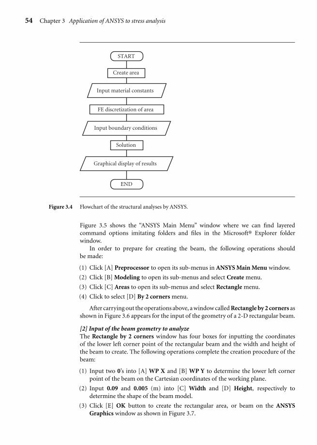
Ch03-H6875.tex 24/11/2006 17: 2 page 54


START

Create area

Input material constants

FE discretization of area

Solution

Input boundary conditions

Graphical display of results

END

Figure 3.4 Flowchart of the structural analyses by ANSYS.

Figure 3.5 shows the “ANSYS Main Menu” window where we can find layeredcommand options imitating folders and files in the Microsoft® Explorer folderwindow.

In order to prepare for creating the beam, the following operations shouldbe made:

(1) Click [A] Preprocessor to open its sub-menus in ANSYS Main Menu window.

(2) Click [B] Modeling to open its sub-menus and select Create menu.

(3) Click [C] Areas to open its sub-menus and select Rectangle menu.

(4) Click to select [D] By 2 corners menu.

After carrying out the operations above, a window called Rectangle by 2 corners asshown in Figure 3.6 appears for the input of the geometry of a 2-D rectangular beam.

[2] Input of the beam geometry to analyzeThe Rectangle by 2 corners window has four boxes for inputting the coordinatesof the lower left corner point of the rectangular beam and the width and height ofthe beam to create. The following operations complete the creation procedure of thebeam:

(1) Input two 0’s into [A] WP X and [B] WP Y to determine the lower left cornerpoint of the beam on the Cartesian coordinates of the working plane.

(2) Input 0.09 and 0.005 (m) into [C] Width and [D] Height, respectively todetermine the shape of the beam model.

(3) Click [E] OK button to create the rectangular area, or beam on the ANSYSGraphics window as shown in Figure 3.7.

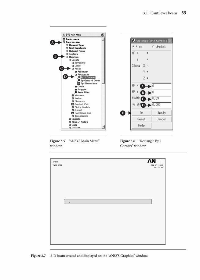
Ch03-H6875.tex 24/11/2006 17: 2 page 55


A

B

C

D

Figure 3.5 “ANSYS Main Menu”

window.

A

B

C

D

E

Figure 3.6 “Rectangle By 2

Corners” window.

Figure 3.7 2-D beam created and displayed on the “ANSYS Graphics” window.

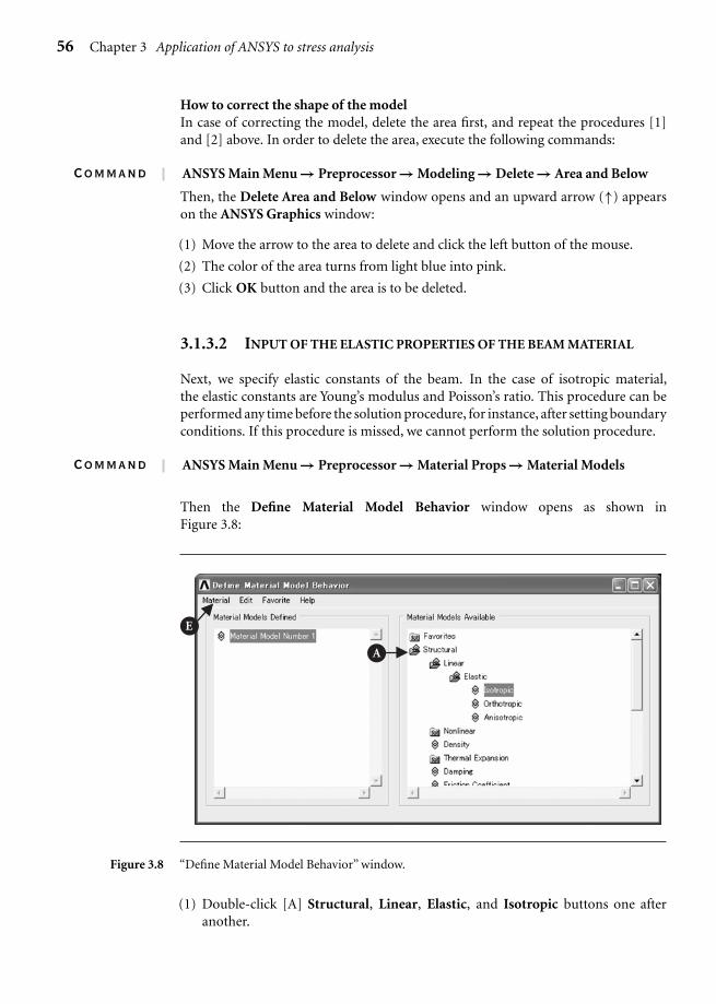
Ch03-H6875.tex 24/11/2006 17: 2 page 56


How to correct the shape of the modelIn case of correcting the model, delete the area first, and repeat the procedures [1]and [2] above. In order to delete the area, execute the following commands:

Command ANSYS Main Menu → Preprocessor → Modeling → Delete → Area and Below

Then, the Delete Area and Below window opens and an upward arrow (↑) appearson the ANSYS Graphics window:

(1) Move the arrow to the area to delete and click the left button of the mouse.

(2) The color of the area turns from light blue into pink.

(3) Click OK button and the area is to be deleted.

3.1.3.2 INPUT OF THE ELASTIC PROPERTIES OF THE BEAM MATERIAL

Next, we specify elastic constants of the beam. In the case of isotropic material,the elastic constants are Young’s modulus and Poisson’s ratio. This procedure can beperformed any time before the solution procedure, for instance, after setting boundaryconditions. If this procedure is missed, we cannot perform the solution procedure.

Command ANSYS Main Menu → Preprocessor → Material Props → Material Models

Then the Define Material Model Behavior window opens as shown inFigure 3.8:

A

E

Figure 3.8 “Define Material Model Behavior” window.

(1) Double-click [A] Structural, Linear, Elastic, and Isotropic buttons one afteranother.

Ch03-H6875.tex 24/11/2006 17: 2 page 57


(2) Input the value of Young’s modulus, 2.1e11 (Pa), and that of Poisson’s ratio, 0.3,into [B] EX and [C] PRXY boxes, and click [D] OK button of the Linear IsotropicProperties for Material Number 1 as shown in Figure 3.9.

B

C

D

Figure 3.9 Input of elastic constants through the “Linear Isotropic Properties for Material Number 1”window.

(3) Exit from the Define Material Model Behavior window by selecting Exit in [E]Material menu of the window (see Figure 3.8).

3.1.3.3 FINITE-ELEMENT DISCRETIZATION OF THE BEAM AREA

Here we will divide the beam area into finite elements. The procedures for finite-element discretization are firstly to select the element type, secondly to input theelement thickness and finally to divide the beam area into elements.

[1] Selection of the element type

Command ANSYS Main Menu → Preprocessor → Element Type → Add/ Edit/Delete

Then the Element Types window opens:

(1) Click [A] Add . . . button to open the Library of Element Types window as shownin Figure 3.11 and select the element type to use.

(2) To select the 8-node isoparametric element, select [B] Structural Mass – Solid.

(3) Select [C] Quad 8node 82 and click [D] OK button to choose the 8-nodeisoparametric element.

(4) Click [E] Options . . . button in the Element Types window as shown in Fig-ure 3.10 to open the PLANE82 element type options window as depicted inFigure 3.12. Select [F] Plane strs w/thk item in the Element behavior box andclick [G] OK button to return to the Element Types window. Click [H] Closebutton to close the window.

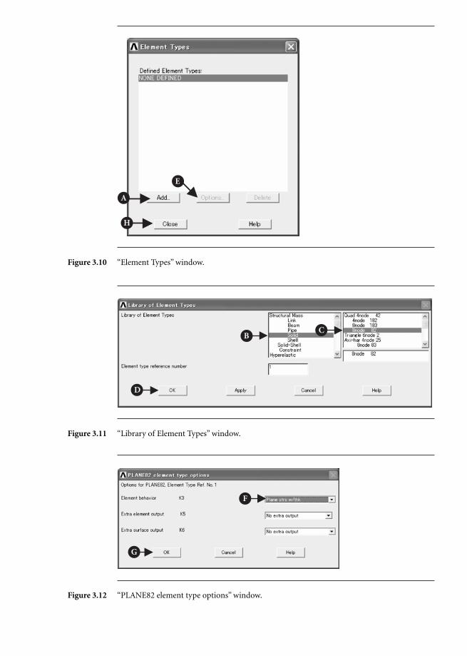
Ch03-H6875.tex 24/11/2006 17: 2 page 58

E

A

H

Figure 3.10 “Element Types” window.

D

BC

Figure 3.11 “Library of Element Types” window.

F

G

Figure 3.12 “PLANE82 element type options” window.

Ch03-H6875.tex 24/11/2006 17: 2 page 59


Figure 3.13 8-node

isoparametric rectangu-

lar element.

A

Figure 3.14 Setting of the

element thickness from the real

constant command.

The 8-node isoparametric element is a rectan-gular element which has four corner nodal pointsand four middle points as shown in Figure 3.13 andcan realize the finite-element analysis with higheraccuracy than the 4-node linear rectangular ele-ment. The beam area is divided into these 8-noderectangular #82 finite elements.

[2] Input of the element thickness

Command ANSYS Main Menu → Preprocessor → RealConstants

Select [A] Real Constants in the ANSYS MainMenu as shown in Figure 3.14.

(1) Click [A] Add/Edit/Delete button to open the Real Constants window as shownin Figure 3.15 and click [B] Add … button.

(2) Then the Element Type for Real Constants window opens (see Figure 3.16). Click[C] OK button.

(3) The Element Type for Real Constants window vanishes and the Real ConstantsSet Number 1. for PLANE82 window appears instead as shown in Figure 3.17.

B

Figure 3.15 “Real Constants” window

before setting the element thickness.

C

Figure 3.16 “Element Type for Real Constants”

window.

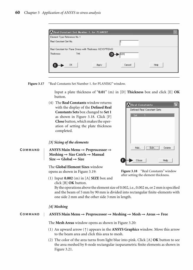
Ch03-H6875.tex 24/11/2006 17: 2 page 60


D

E

Figure 3.17 “Real Constants Set Number 1. for PLANE82” window.

Input a plate thickness of “0.01” (m) in [D] Thickness box and click [E] OKbutton.

F

Figure 3.18 “Real Constants” windowafter setting the element thickness.

(4) The Real Constants window returnswith the display of the Defined RealConstants Sets box changed to Set 1as shown in Figure 3.18. Click [F]Close button, which makes the oper-ation of setting the plate thicknesscompleted.

[3] Sizing of the elements

Command ANSYS Main Menu → Preprocessor →Meshing → Size Cntrls → ManualSize → Global → Size

The Global Element Sizes windowopens as shown in Figure 3.19:

(1) Input 0.002 (m) in [A] SIZE box andclick [B] OK button.By the operations above the element size of 0.002, i.e., 0.002 m, or 2 mm is specifiedand the beam of 5 mm by 90 mm is divided into rectangular finite-elements withone side 2 mm and the other side 3 mm in length.

[4] Meshing

Command ANSYS Main Menu → Preprocessor → Meshing → Mesh → Areas → Free

The Mesh Areas window opens as shown in Figure 3.20:

(1) An upward arrow (↑) appears in the ANSYS Graphics window. Move this arrowto the beam area and click this area to mesh.

(2) The color of the area turns from light blue into pink. Click [A] OK button to seethe area meshed by 8-node rectangular isoparametric finite elements as shown inFigure 3.21.

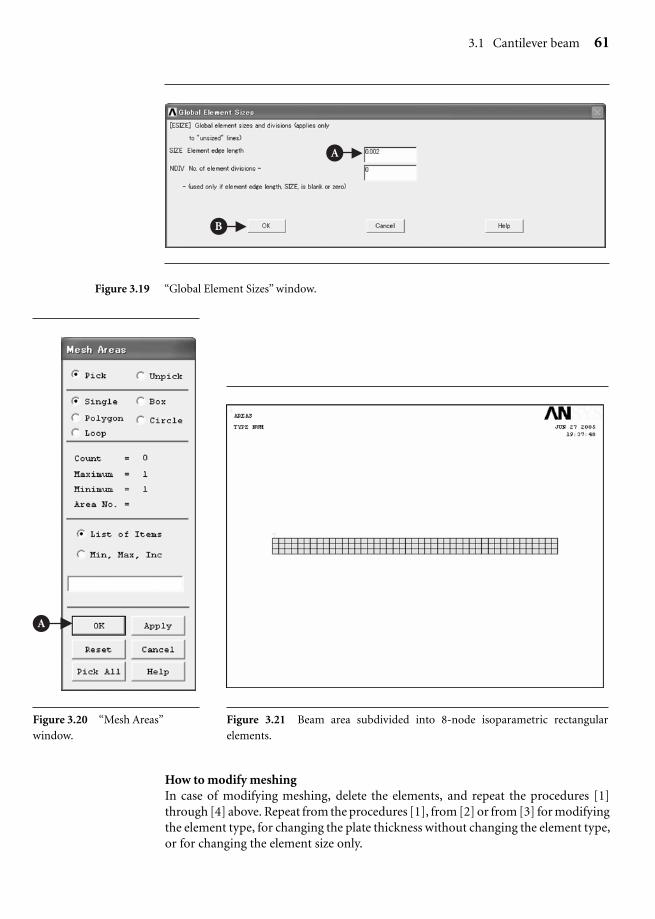
Ch03-H6875.tex 24/11/2006 17: 2 page 61


A

B

Figure 3.19 “Global Element Sizes” window.

A

Figure 3.20 “Mesh Areas”

window.

Figure 3.21 Beam area subdivided into 8-node isoparametric rectangular

elements.

How to modify meshingIn case of modifying meshing, delete the elements, and repeat the procedures [1]through [4] above. Repeat from the procedures [1], from [2] or from [3] for modifyingthe element type, for changing the plate thickness without changing the element type,or for changing the element size only.

Ch03-H6875.tex 24/11/2006 17: 2 page 62


In order to delete the elements, execute the following commands:

Command ANSYS Main Menu → Preprocessor → Meshing → Clear → Areas

The Clear Areas window opens:

(1) An upward arrow (↑) appears in the ANSYS Graphics window. Move this arrowto the beam area and click this area.

(2) The color of the area turns from light blue into pink. Click OK button to delete theelements from the beam area. After this operation, the area disappears from thedisplay. Execute the following commands to replot the area.

Command ANSYS Utility Menu → Plot → Areas

3.1.3.4 INPUT OF BOUNDARY CONDITIONS

Here we will impose constraint and loading conditions on nodes of the beam model.Display the nodes first to define the constraint and loading conditions.

[1] Nodes display

Command ANSYS Utility Menu → Plot → Nodes

The nodes are plotted in the ANSYS Graphics window opens as shown in Figure 3.22.

Figure 3.22 Plots of nodes.

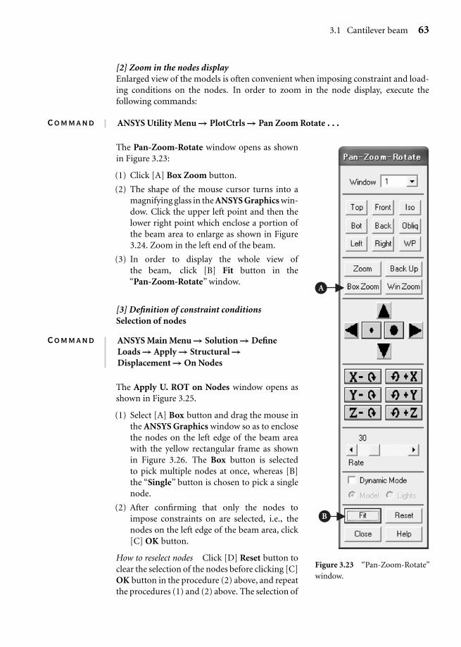
Ch03-H6875.tex 24/11/2006 17: 2 page 63


[2] Zoom in the nodes displayEnlarged view of the models is often convenient when imposing constraint and load-ing conditions on the nodes. In order to zoom in the node display, execute thefollowing commands:

Command ANSYS Utility Menu → PlotCtrls → Pan Zoom Rotate . . .

A

B

Figure 3.23 “Pan-Zoom-Rotate”

window.

The Pan-Zoom-Rotate window opens as shownin Figure 3.23:

(1) Click [A] Box Zoom button.

(2) The shape of the mouse cursor turns into amagnifying glass in the ANSYS Graphics win-dow. Click the upper left point and then thelower right point which enclose a portion ofthe beam area to enlarge as shown in Figure3.24. Zoom in the left end of the beam.

(3) In order to display the whole view ofthe beam, click [B] Fit button in the“Pan-Zoom-Rotate” window.

[3] Definition of constraint conditionsSelection of nodes

Command ANSYS Main Menu → Solution → DefineLoads → Apply → Structural →Displacement → On Nodes

The Apply U. ROT on Nodes window opens asshown in Figure 3.25.

(1) Select [A] Box button and drag the mouse inthe ANSYS Graphics window so as to enclosethe nodes on the left edge of the beam areawith the yellow rectangular frame as shownin Figure 3.26. The Box button is selectedto pick multiple nodes at once, whereas [B]the “Single” button is chosen to pick a singlenode.

(2) After confirming that only the nodes toimpose constraints on are selected, i.e., thenodes on the left edge of the beam area, click[C] OK button.

How to reselect nodes Click [D] Reset button toclear the selection of the nodes before clicking [C]OK button in the procedure (2) above, and repeatthe procedures (1) and (2) above. The selection of

Ch03-H6875.tex 24/11/2006 17: 2 page 64


(1) Click the upper left point.

(2) Click the lower right point.

Figure 3.24 Magnification of an observation area.

AB

E

C

D

Figure 3.25 “Apply U. ROT on Nodes” window.

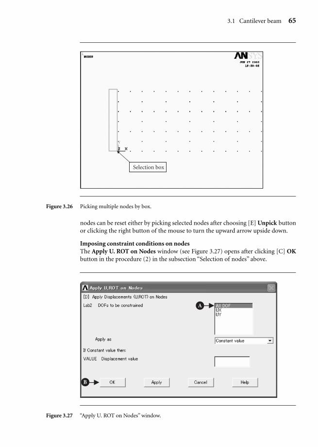
Ch03-H6875.tex 24/11/2006 17: 2 page 65


Selection box

Figure 3.26 Picking multiple nodes by box.

nodes can be reset either by picking selected nodes after choosing [E] Unpick buttonor clicking the right button of the mouse to turn the upward arrow upside down.

Imposing constraint conditions on nodesThe Apply U. ROT on Nodes window (see Figure 3.27) opens after clicking [C] OKbutton in the procedure (2) in the subsection “Selection of nodes” above.

A

B

Figure 3.27 “Apply U. ROT on Nodes” window.

Ch03-H6875.tex 24/11/2006 17: 2 page 66


(1) In case of selecting [A] ALL DOF, the nodes are to be clamped, i.e., the displace-ments are set to zero in the directions of the x- and y-axes. Similarly, the selectionof UX makes the displacement in the x-direction equal to zero and the selectionof UY makes the displacement in the y-direction equal to zero.

(2) Click [B] OK button and blue triangular symbols, which denote the clampingconditions, appear in the ANSYS Graphics window as shown in Figure 3.28.The upright triangles indicate that each node to which the triangular symbol isattached is fixed in the y-direction, whereas the tilted triangles indicate the fixedcondition in the x-direction.

Figure 3.28 Imposing the clamping conditions on nodes.

How to clear constraint conditions

Command ANSYS Main Menu → Solution → Define Loads → Delete → Structural →Displacement → On Nodes

The Delete Node Constrai… window opens.

(1) Click Pick All button to delete the constraint conditions of all the nodes thatthe constraint conditions are imposed. Select Single button and pick a particularnode by the upward arrow in the ANSYS Graphics window and click OK button.

(2) The Delete Node constraints window appears. Select ALL DOF and click OKbutton to delete the constraint conditions both in the x- and y-directions. SelectUX and UY to delete the constraints in the x- and the y-directions, respectively.

[4] Imposing boundary conditions on nodesBefore imposing load conditions, click Fit button in the Pan-Zoom-Rotate window(see Figure 3.23) to get the whole view of the area and then zoom in the right end ofthe beam area for ease of the following operations.

Ch03-H6875.tex 24/11/2006 17: 2 page 67


Selection of the nodes(1) Pick the node at a point where x = 0.08 m and y = 0.005 m for this purpose, click

Command ANSYS Utility Menu → PlotCtrls → Numbering . . .

consecutively to open the Plot Numbering Controls window as shown in Figure 3.29.

A

B

Figure 3.29 “Plot Numbering Controls” window.

(2) Click [A] NODE � Off box to change it to �✓ On box.

(3) Click [B] OK button to display node numbers adjacent to corresponding nodesin the ANSYS Graphics window as shown in Figure 3.30.

(4) To delete the node numbers, click [A] NODE �✓ On box again to change it to

� Off box.

(5) Execute the following commands:

Command ANSYS Utility Menu → List → Nodes . . .

and the Sort NODE Listing window opens (see Figure 3.31). Select [A] Coordinatesonly button and then click [B] OK button.

(6) The“NLIST Command”window opens as shown in Figure 3.32. Find the numberof the node having the coordinates x = 0.08 m and y = 0.005 m, namely node #108in Figure 3.32.

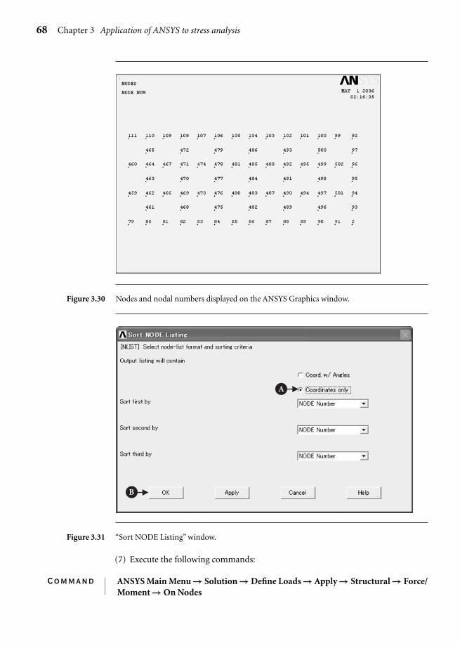
Ch03-H6875.tex 24/11/2006 17: 2 page 68


Figure 3.30 Nodes and nodal numbers displayed on the ANSYS Graphics window.

A

B

Figure 3.31 “Sort NODE Listing” window.

(7) Execute the following commands:

Command ANSYS Main Menu → Solution → Define Loads → Apply → Structural → Force/Moment → On Nodes

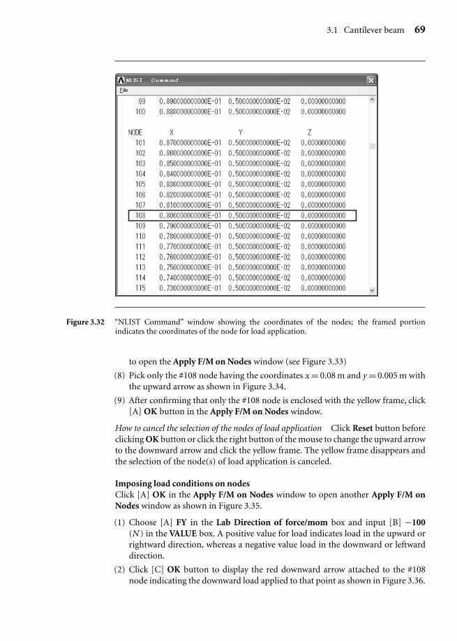
Ch03-H6875.tex 24/11/2006 17: 2 page 69


Figure 3.32 “NLIST Command” window showing the coordinates of the nodes; the framed portionindicates the coordinates of the node for load application.

to open the Apply F/M on Nodes window (see Figure 3.33)

(8) Pick only the #108 node having the coordinates x = 0.08 m and y = 0.005 m withthe upward arrow as shown in Figure 3.34.

(9) After confirming that only the #108 node is enclosed with the yellow frame, click[A] OK button in the Apply F/M on Nodes window.

How to cancel the selection of the nodes of load application Click Reset button beforeclicking OK button or click the right button of the mouse to change the upward arrowto the downward arrow and click the yellow frame. The yellow frame disappears andthe selection of the node(s) of load application is canceled.

Imposing load conditions on nodesClick [A] OK in the Apply F/M on Nodes window to open another Apply F/M onNodes window as shown in Figure 3.35.

(1) Choose [A] FY in the Lab Direction of force/mom box and input [B] −100(N) in the VALUE box. A positive value for load indicates load in the upward orrightward direction, whereas a negative value load in the downward or leftwarddirection.

(2) Click [C] OK button to display the red downward arrow attached to the #108node indicating the downward load applied to that point as shown in Figure 3.36.

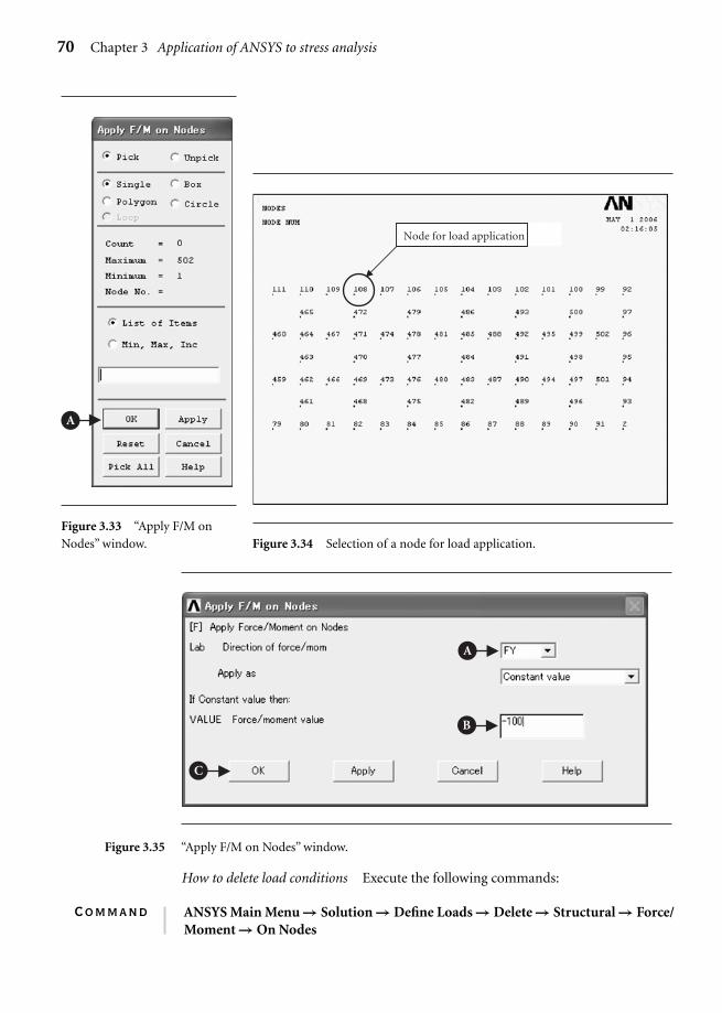
Ch03-H6875.tex 24/11/2006 17: 2 page 70


A

Figure 3.33 “Apply F/M on

Nodes” window.

Node for load application

Figure 3.34 Selection of a node for load application.

A

B

C

Figure 3.35 “Apply F/M on Nodes” window.

How to delete load conditions Execute the following commands:

Command ANSYS Main Menu → Solution → Define Loads → Delete → Structural → Force/Moment → On Nodes

Ch03-H6875.tex 24/11/2006 17: 2 page 71


Figure 3.36 Display of the load application on a node by arrow symbol.

A

B

Figure 3.37 “Delete F/M on Nodes” window.

to open the Delete F/M on Nodes window (see Figure 3.37). Choose [A] FY or ALLin the Lab Force/moment to be deleted and click OK button to delete the downwardload applied to the #108 node.

3.1.3.5 SOLUTION PROCEDURES

Command ANSYS Main Menu → Solution → Solve → Current LS

The Solve Current Load Step and /STATUS Command windows appear as shown inFigures 3.38 and 3.39, respectively.

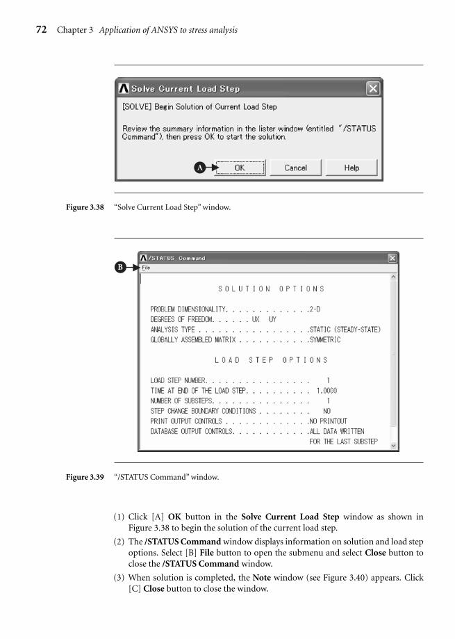
Ch03-H6875.tex 24/11/2006 17: 2 page 72


A

Figure 3.38 “Solve Current Load Step” window.

B

Figure 3.39 “/STATUS Command” window.

(1) Click [A] OK button in the Solve Current Load Step window as shown inFigure 3.38 to begin the solution of the current load step.

(2) The /STATUS Command window displays information on solution and load stepoptions. Select [B] File button to open the submenu and select Close button toclose the /STATUS Command window.

(3) When solution is completed, the Note window (see Figure 3.40) appears. Click[C] Close button to close the window.

Ch03-H6875.tex 24/11/2006 17: 2 page 73


C

Figure 3.40 “Note” window.

3.1.3.6 GRAPHICAL REPRESENTATION OF THE RESULTS

[1] Contour plot of displacements

Command ANSYS Main Menu → General Postproc → Plot Results → Contour Plot → NodalSolution

The Contour Nodal Solution Data window opens as shown in Figure 3.41.

A

B

C

D

Figure 3.41 “Contour Nodal Solution Data” window.

Ch03-H6875.tex 24/11/2006 17: 2 page 74


(1) Select [A] DOF Solution and [B] Y-Component of displacement.

(2) Select [C] Deformed shape with undeformed edge in the Undisplaced shapekey box to compare the shapes of the beam before and after deformation.

Figure 3.42 Contour map representation of the distribution of displacement in the y- or vertical direction.

(3) Click [D] OK button to display the contour of the y-component of displacement,or the deflection of the beam in the ANSYS Graphics window (see Figure 3.42).The DMX value shown in the Graphics window indicates the maximum deflectionof the beam.

[2] Contour plot of stresses(1) Select [A] Stress and [B] X-Component of stress as shown in Figure 3.43.

(2) Click [C] OK button to display the contour of the x-component of stress, or thebending stress in the beam in the ANSYS Graphics window (see Figure 3.44). TheSMX and SMN values shown in the Graphics window indicate the maximum andthe minimum stresses in the beam, respectively.

(3) Click [D] Additional Options bar to open additional option items to choose.Select [E] All applicable in the Number of facets per element edge box tocalculate stresses and strains at middle points of the elements.

Ch03-H6875.tex 24/11/2006 17: 2 page 75

A

B

D

C

E

Figure 3.43 “Contour Nodal Solution Data” window.

Figure 3.44 Contour map representation of the distribution of normal stress in the x- or horizontaldirection.

Ch03-H6875.tex 24/11/2006 17: 2 page 76


3.1.4 Comparison of FEM results with experimental ones

Figure 3.45 compares longitudinal stress distributions obtained by ANSYS with thoseby experiments and by the elementary beam theory. The results obtained by threedifferent methods agree well with one another. As the applied load increases, however,errors among the three groups of the results become larger, especially at the clampedend. This tendency arises from the fact that the clamped condition can be hardlyrealized in the strict sense.

20 30 40 50 60�300

�200

�100

0

100

200

300

x-coordinate, x (mm)

Lon

gitu

din

al s

tres

s, σ

, (M

Pa)

100 N

150 N

P�200 N

200 N

150 N

P�100 N

ANSYSExperimentTheory

Figure 3.45 Comparison of longitudinal stress distributions obtained by ANSYS with those by experimentsand by the elementary beam theory.

3.1.5 Problems to solve

PROBLEM 3.1

Change the point of load application and the intensity of the applied load in thecantilever beam model shown in Figure 3.3 and calculate the maximum deflection.

PROBLEM 3.2

Calculate the maximum deflection in a beam clamped at the both ends as shown inFigure P3.2 where the thickness of the beam in the direction perpendicular to thepage surface is 10 mm.

(Answer: 0.00337 mm)

PROBLEM 3.3

Calculate the maximum deflection in a beam simply supported at the both ends asshown in Figure P3.3 where the thickness of the beam in the direction perpendicularto the page surface is 10 mm.


Ch03-H6875.tex 24/11/2006 17: 2 page 77


100 mm

100 N50 mm

10 mm

Figure P3.2 A beam clamped at the both ends and subjected to a concentrated force of 100 N at the centerof the span.

100 mm

100 N50 mm

10 mm

10 mm

10 mm

Figure P3.3 A beam simply supported at the both ends and subjected to a concentrated force of 100 N atthe center of the span.

PROBLEM 3.4

Calculate the maximum deflection in a beam shown in Figure P3.4 where the thicknessof the beam in the direction perpendicular to the page surface is 10 mm. Choose anelement size of 1 mm.

(Answer: 0.00337 mm)Note that the beam shown in Figure P3.2 is bilaterally symmetric so that the

x-component of the displacement (DOF X) is zero at the center of the beam span. Ifthe beam shown in Figure P3.2 is cut at the center of the span and the finite-elementcalculation is made for only the left half of the beam by applying a half load of50 N to its right end which is fixed in the x-direction but is deformed freely in they-direction as shown in Figure P3.4, the solution obtained is the same as that for theleft half of the beam in Problem 3.2. Problem 3.2 can be solved by its half modelas shown in Figure P3.4. A half model can achieve the efficiency of finite-elementcalculations.

Ch03-H6875.tex 24/11/2006 17: 2 page 78


50 mm

50 N

10 mm

DOF X

Figure P3.4 A half model of the beam in Problem 3.2.

50 mm

50 N10 mm

10 mm

Figure P3.5 A half model of the beam in Problem 3.3.

PROBLEM 3.5

Calculate the maximum deflection in a beam shown in Figure P3.5 where the thicknessof the beam in the direction perpendicular to the page surface is 10 mm. This beamis the half model of the beam of Problem 3.3.


PROBLEM 3.6

Calculate the maximum value of the von Mises stress in the stepped beam as shown inFigure P3.6 where Young’s modulus E = 210 GPa, Poisson’s ratio ν = 0.3, the elementsize is 2 mm and the beam thickness is 10 mm. Refer to the Appendix to create thestepped beam. The von Mises stress σeq is sometimes called the equivalent stress or

Ch03-H6875.tex 24/11/2006 17: 2 page 79


the effective stress and is expressed by the following formula:

σeq = 1√2

√(σx − σy)2 + (σy − σz)2 + (σz − σx)2 + 6(τ2

xy + τ2yz + τ2

zx) (P3.6)

in three-dimensional elasticity problems. It is often considered that a material yieldswhen the value of the von Mises stress reaches the yield stress of the material σY whichis determined by the uniaxial tensile tests of the material.

(Answer: 40.8 MPa)

50 mm

20 mm

10 mm

100 mm

100 N

Figure P3.6 A stepped cantilever beam subjected to a concentrated force of 100 N at the free end.

PROBLEM 3.7

Calculate the maximum value of the von Mises stress in the stepped beam with arounded fillet as shown in Figure P3.7 where Young’s modulus E = 210 GPa, Pois-son’s ratio ν = 0.3, the element size is 2 mm and the beam thickness is 10 mm. Referto the Appendix to create the stepped beam with a rounded fillet.

(Answer: 30.2 MPa)

50 mm

20 mm10 mm

100 mm

100 NR10 mm

Figure P3.7 A stepped cantilever beam with a rounded fillet subjected to a concentrated force of 100 N atthe free end.

Ch03-H6875.tex 24/11/2006 17: 2 page 80


A

Figure 3.46 “Add Areas”

window.

Appendix: procedures forcreating stepped beams

A3.1 Creation of a stepped beam

A stepped beam as shown in Figure P3.6 can becreated by adding two rectangular areas of differentsizes:

(1) Create two rectangular areas of different sizes,say 50 mm by 20 mm with WP X = −50 mmand WP Y = −10 mm, and 60 mm by 10 mmwith WP X = −10 mm and WP Y = −10 mm,following operations described in 3.1.3.1.

(2) Select the Boolean operation of adding areasas follows to open the Add Areas window (seeFigure 3.46)

Command ANSYS Main Menu → Preprocessor →Modeling → Operate → Booleans →Add → Areas

(3) Pick all the areas to add by the upward arrow.

(4) The color of the areas picked turns from lightblue into pink (see Figure 3.47). Click [A] OKbutton to add the two rectangular areas to createa stepped beam area as shown in Figure 3.48.

Figure 3.47 Two rectangular areas of different sizes to be added to create a stepped beam area.

Ch03-H6875.tex 24/11/2006 17: 2 page 81


Figure 3.48 A stepped beam area created by adding two rectangle areas.

A3.1.1 HOW TO CANCEL THE SELECTION OF AREAS

Click Reset button or click the right button of the mouse to change the upward arrowto the downward arrow and click the area(s) to pick. The color of the unpicked area(s)turns pink into light blue and the selection of the area(s) is canceled.

A3.2 Creation of a stepped beam with a rounded fillet

A stepped beam with a rounded fillet as shown in Figure P3.7 can be created bysubtracting a smaller rectangular area and a solid circle from a larger rectangulararea:

(1) Create a larger rectangular area of 100 mm by 20 mm with WP X = −100 mmand WP Y = −10 mm, a smaller rectangular area of, say 50 mm by 15 mm withWP X = 10 mm and WP Y = 0 mm, and a solid circular area having a diameterof 10 mm with WP X = 10 mm and WP Y = 10 mm as shown in Figure 3.49. Thesolid circular area can be created by executing the following operation:

Command ANSYS Main Menu → Preprocessor → Modeling → Create → Areas →Circle → Solid Circle

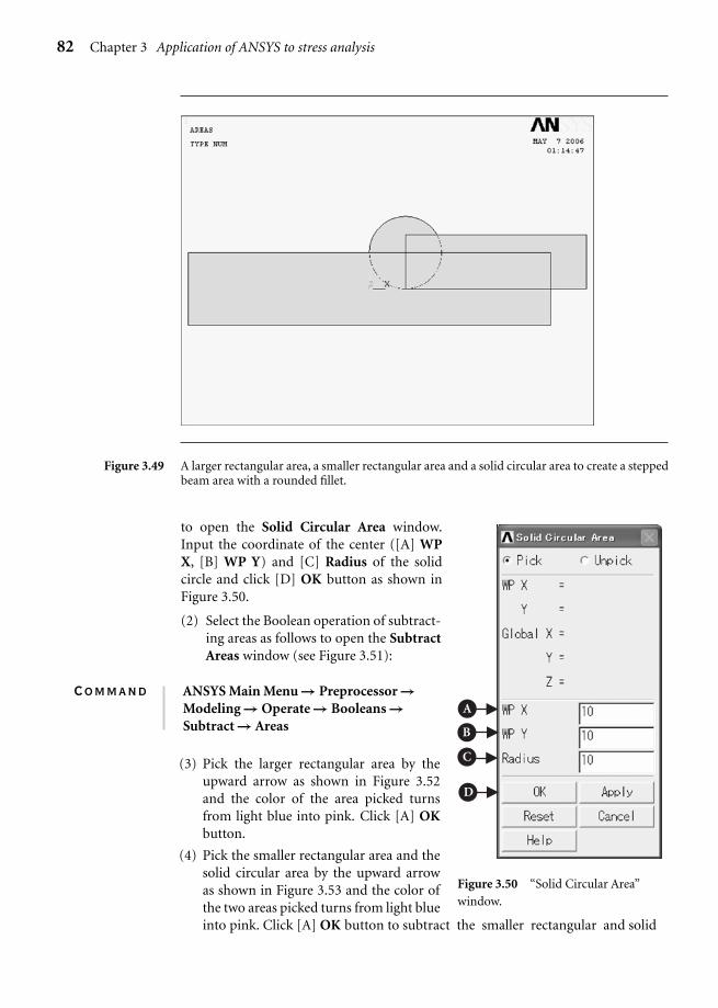
Ch03-H6875.tex 24/11/2006 17: 2 page 82


Figure 3.49 A larger rectangular area, a smaller rectangular area and a solid circular area to create a steppedbeam area with a rounded fillet.

to open the Solid Circular Area window.Input the coordinate of the center ([A] WPX, [B] WP Y) and [C] Radius of the solidcircle and click [D] OK button as shown inFigure 3.50.

A

B

C

D

Figure 3.50 “Solid Circular Area”

window.

(2) Select the Boolean operation of subtract-ing areas as follows to open the SubtractAreas window (see Figure 3.51):

Command ANSYS Main Menu → Preprocessor →Modeling → Operate → Booleans →Subtract → Areas

(3) Pick the larger rectangular area by theupward arrow as shown in Figure 3.52and the color of the area picked turnsfrom light blue into pink. Click [A] OKbutton.

(4) Pick the smaller rectangular area and thesolid circular area by the upward arrowas shown in Figure 3.53 and the color ofthe two areas picked turns from light blueinto pink. Click [A] OK button to subtract the smaller rectangular and solid

Ch03-H6875.tex 24/11/2006 17: 2 page 83

A

Figure 3.51 “Subtract Areas”

window. Figure 3.52 The larger rectangular area picked.

Figure 3.53 The smaller rectangular area and the solid circular area picked to be subtracted from the largerrectangular area to create a stepped beam area with a rounded fillet.

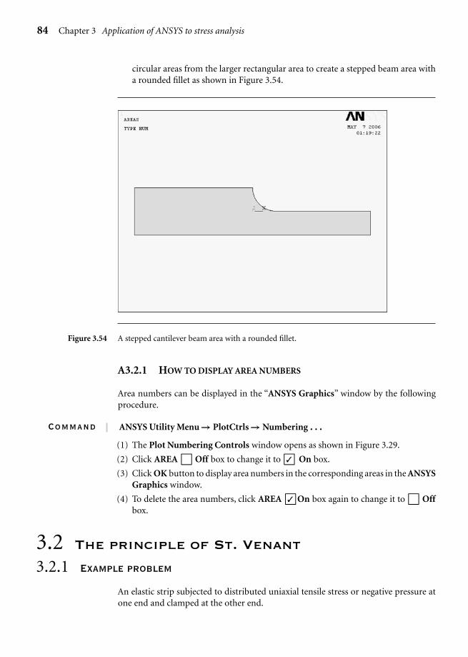
Ch03-H6875.tex 24/11/2006 17: 2 page 84


circular areas from the larger rectangular area to create a stepped beam area witha rounded fillet as shown in Figure 3.54.

Figure 3.54 A stepped cantilever beam area with a rounded fillet.

A3.2.1 HOW TO DISPLAY AREA NUMBERS

Area numbers can be displayed in the “ANSYS Graphics” window by the followingprocedure.

Command ANSYS Utility Menu → PlotCtrls → Numbering . . .

(1) The Plot Numbering Controls window opens as shown in Figure 3.29.

(2) Click AREA � Off box to change it to �✓ On box.

(3) Click OK button to display area numbers in the corresponding areas in the ANSYSGraphics window.

(4) To delete the area numbers, click AREA �✓ On box again to change it to � Offbox.

3.2 The principle of St. Venant

3.2.1 Example problem

An elastic strip subjected to distributed uniaxial tensile stress or negative pressure atone end and clamped at the other end.

Ch03-H6875.tex 24/11/2006 17: 2 page 85

3.2 The principle of St. Venant 85

Perform an FEM analysis of a 2-D elastic strip subjected to a distributed stressin the longitudinal direction at one end and clamped at the other end (shown inFigure 3.55 below) and calculate the stress distributions along the cross sections atdifferent distances from the loaded end in the strip.

Triangular distribution of stress σ0

200 mm

20 m

m

10 MPa

Figure 3.55 A 2-D elastic strip subjected to a distributed force in the longitudinal direction at one end andclamped at the other end.


Geometry: length l = 200 mm, height h = 20 mm, thickness b = 10 mm.Material: mild steel having Young’s modulus E = 210 GPa and Poisson’s ratio ν = 0.3.Boundary conditions: The elastic strip is subjected to a triangular distribution ofstress in the longitudinal direction at the right end and clamped to a rigid wall at theleft end.



Command ANSYS Main Menu → Preprocessor → Modeling → Create → Areas →Rectangle → By 2 Corners

(1) Input two 0’s into the “WP X” and “WP Y” boxes in the “Rectangle by 2 Cor-ners” window to determine the lower left corner point of the elastic strip on theCartesian coordinates of the working plane.

(2) Input 200 and 20 (mm) into the Width and Height boxes, respectively, todetermine the shape of the elastic strip model.

(3) Click the OK button to create the rectangular area, or beam on the ANSYSGraphics window.

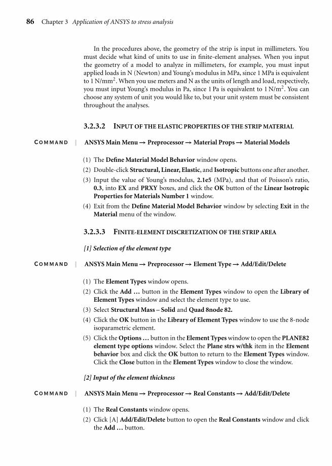
Ch03-H6875.tex 24/11/2006 17: 2 page 86


In the procedures above, the geometry of the strip is input in millimeters. Youmust decide what kind of units to use in finite-element analyses. When you inputthe geometry of a model to analyze in millimeters, for example, you must inputapplied loads in N (Newton) and Young’s modulus in MPa, since 1 MPa is equivalentto 1 N/mm2. When you use meters and N as the units of length and load, respectively,you must input Young’s modulus in Pa, since 1 Pa is equivalent to 1 N/m2. You canchoose any system of unit you would like to, but your unit system must be consistentthroughout the analyses.

3.2.3.2 INPUT OF THE ELASTIC PROPERTIES OF THE STRIP MATERIAL


(1) The Define Material Model Behavior window opens.

(2) Double-click Structural, Linear, Elastic, and Isotropic buttons one after another.

(3) Input the value of Young’s modulus, 2.1e5 (MPa), and that of Poisson’s ratio,0.3, into EX and PRXY boxes, and click the OK button of the Linear IsotropicProperties for Materials Number 1 window.

(4) Exit from the Define Material Model Behavior window by selecting Exit in theMaterial menu of the window.

3.2.3.3 FINITE-ELEMENT DISCRETIZATION OF THE STRIP AREA


Command ANSYS Main Menu → Preprocessor → Element Type → Add/Edit/Delete

(1) The Element Types window opens.

(2) Click the Add … button in the Element Types window to open the Library ofElement Types window and select the element type to use.

(3) Select Structural Mass – Solid and Quad 8node 82.

(4) Click the OK button in the Library of Element Types window to use the 8-nodeisoparametric element.

(5) Click the Options … button in the Element Types window to open the PLANE82element type options window. Select the Plane strs w/thk item in the Elementbehavior box and click the OK button to return to the Element Types window.Click the Close button in the Element Types window to close the window.


Command ANSYS Main Menu → Preprocessor → Real Constants → Add/Edit/Delete

(1) The Real Constants window opens.

(2) Click [A] Add/Edit/Delete button to open the Real Constants window and clickthe Add … button.

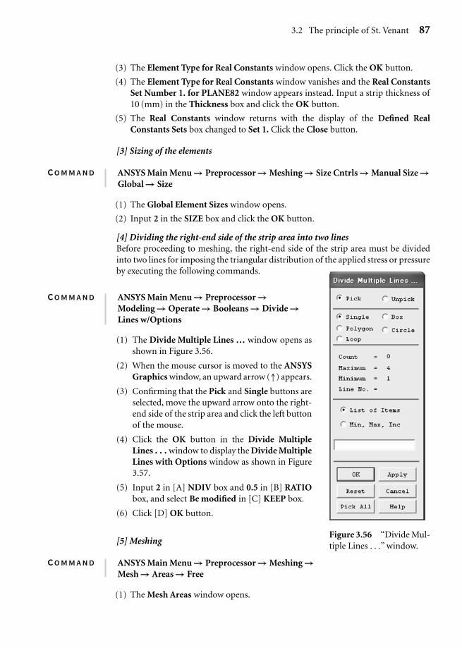
Ch03-H6875.tex 24/11/2006 17: 2 page 87


(3) The Element Type for Real Constants window opens. Click the OK button.

(4) The Element Type for Real Constants window vanishes and the Real ConstantsSet Number 1. for PLANE82 window appears instead. Input a strip thickness of10 (mm) in the Thickness box and click the OK button.

(5) The Real Constants window returns with the display of the Defined RealConstants Sets box changed to Set 1. Click the Close button.


Command ANSYS Main Menu → Preprocessor → Meshing → Size Cntrls → Manual Size →Global → Size

(1) The Global Element Sizes window opens.

(2) Input 2 in the SIZE box and click the OK button.

[4] Dividing the right-end side of the strip area into two linesBefore proceeding to meshing, the right-end side of the strip area must be dividedinto two lines for imposing the triangular distribution of the applied stress or pressureby executing the following commands.

Command

Figure 3.56 “Divide Mul-tiple Lines . . .” window.

ANSYS Main Menu → Preprocessor →Modeling → Operate → Booleans → Divide →Lines w/Options

(1) The Divide Multiple Lines … window opens asshown in Figure 3.56.

(2) When the mouse cursor is moved to the ANSYSGraphics window, an upward arrow (↑) appears.

(3) Confirming that the Pick and Single buttons areselected, move the upward arrow onto the right-end side of the strip area and click the left buttonof the mouse.

(4) Click the OK button in the Divide MultipleLines . . . window to display the Divide MultipleLines with Options window as shown in Figure3.57.

(5) Input 2 in [A] NDIV box and 0.5 in [B] RATIObox, and select Be modified in [C] KEEP box.

(6) Click [D] OK button.

[5] Meshing

Command ANSYS Main Menu → Preprocessor → Meshing →Mesh → Areas → Free

(1) The Mesh Areas window opens.

Ch03-H6875.tex 24/11/2006 17: 2 page 88


A

B

C

D

Figure 3.57 “Divide Multiple Lines with Options” window.

(2) The upward arrow appears in the ANSYS Graphics window. Move this arrow tothe elastic strip area and click this area.

(3) The color of the area turns from light blue into pink. Click the OK button to seethe area meshed by 8-node rectangular isoparametric finite elements.


[1] Imposing constraint conditions on the left end of the strip

Command ANSYS Main Menu → Solution → Define Loads → Apply → Structural →Displacement → On Lines

(1) The Apply U. ROT on Lines window opens and the upward arrow appears whenthe mouse cursor is moved to the ANSYS Graphics window.

(2) Confirming that the Pick and Single buttons are selected, move the upward arrowonto the left-end side of the strip area and click the left button of the mouse.

(3) Click the OK button in the Apply U. ROT on Lines window to display anotherApply U. ROT on Lines window.

(4) Select ALL DOF in the Lab2 box and click OK button in the Apply U. ROT onLines window.

[2] Imposing a triangular distribution of applied stress on the right end of the stripDistributed load or stress can be defined by pressure on lines and the triangulardistribution of applied load can be defined as the composite of two linear distributions

Ch03-H6875.tex 24/11/2006 17: 2 page 89


of pressure which are symmetric to each other with respect to the center line of thestrip area.

Command ANSYS Main Menu → Solution → Define Loads → Apply → Structural →Pressure → On Lines

Figure 3.58 “Apply PRES on Lines”window for picking the linesto which pressure is applied.

(1) The Apply PRES on Lines window opens (seeFigure 3.58) and the upward arrow appearswhen the mouse cursor is moved to the ANSYSGraphics window.

(2) Confirming that the Pick and Single buttons areselected, move the upward arrow onto the upperline of the right-end side of the strip area andclick the left button of the mouse. Then, click theOK button. Remember that the right-end sideof the strip area was divided into two lines inProcedure [4] in the preceding Section 3.2.3.3.

(3) Another Apply PRES on Lines window opens(see Figure 3.59). Select Constant value in [A][SFL] Apply PRES on lines as a box and input[B] −10 (MPa) in VALUE Load PRES value boxand [C] 0 (MPa) in Value box.

(4) Click [D] OK button in the window to definea linear distribution of pressure on the upperline which is zero at the upper right corner and−10 (MPa) at the center of the right-end side ofthe strip area (see Figure 3.60).

(5) For the lower line of the right-end side of the striparea, repeat the commands above and Procedures(2) through (4).

(6) Select Constant value in [A] [SFL] Apply PRES on lines as a box and input [B]0 (MPa) in VALUE Load PRES value box and [C] −10 (MPa) in Value box asshown in Figure 3.61. Note that the values to input in the lower two boxes in theApply PRES on Lines window is interchanged, since the distributed pressure onthe lower line of the right-end side of the strip area is symmetric to that on theupper line with respect to the center line of the strip area.

(7) Click [D] OK button in the window shown in Figure 3.60 to define a lineardistribution of pressure on the lower line which is −10 MPa at the center andzero at the lower right corner of the right-end side of the strip area as shown inFigure 3.62.



Ch03-H6875.tex 24/11/2006 17: 2 page 90


A

B

C

D

Figure 3.59 “Apply PRES on Lines” window for applying linearly distributed pressure to the upper half ofthe right end of the elastic strip.

Figure 3.60 Linearly distributed negative pressure applied to the upper half of the right-end side of theelastic strip.

Ch03-H6875.tex 24/11/2006 17: 2 page 91


A

B

C

D

Figure 3.61 “Apply PRES on Lines” window for applying linearly distributed pressure to the lower half ofthe right end of the elastic strip.

Figure 3.62 Triangular distribution of pressure applied to the right end of the elastic strip.

(1) The Solve Current Load Step and /STATUS Command windows appear.

(2) Click the OK button in the Solve Current Load Step window to begin the solutionof the current load step.

Ch03-H6875.tex 24/11/2006 17: 2 page 92


(3) Select the File button in /STATUS Command window to open the submenu andselect the Close button to close the /STATUS Command window.

(4) When solution is completed, the Note window appears. Click the Close buttonto close the “Note” window.

3.2.3.6 CONTOUR PLOT OF STRESS

Command ANSYS Main Menu → General Postproc → Plot Results → Contour Plot → NodalSolution

(1) The Contour Nodal Solution Data window opens.

(2) Select Stress and X-Component of stress.

(3) Click the OK button to display the contour of the x-component of stress in theelastic strip in the ANSYS Graphics window as shown in Figure 3.63.

Figure 3.63 Contour of the x-component of stress in the elastic strip showing uniform stress distributionat one width or larger distance from the right end of the elastic strip to which triangulardistribution of pressure is applied.

3.2.4 Discussion

Figure 3.64 shows the variations of the longitudinal stress distribution in the crosssection with the x-position of the elastic strip. At the right end of the strip, or at

Ch03-H6875.tex 24/11/2006 17: 2 page 93

3.3 Stress concentration due to elliptic holes 93

0 5 100

5

10

15

20

x (mm)200190180100

Longitudinal stress, σx (MPa)

y-co

ordi

nat

e, y

(m

m)

Figure 3.64 Variations of the longitudinal stress distribution in the cross section with the x-position of theelastic strip.

x = 200 mm, the distribution of the applied longitudinal stress takes the triangularshape which is zero at the upper and lower corners and 10 MPa at the center of thestrip. The longitudinal stress distribution varies as the distance of the cross sectionfrom the right end of the strip increases, and the distribution becomes almost uniformat x = 180 mm, i.e., at one width distance from the end of the stress application. Thetotal amount of stress in any cross section is the same, i.e., 1 kN in the strip and, stressis uniformly distributed and the magnitude of stress becomes 5 MPa at any crosssection at one width or larger distance from the end of the stress application.

The above result is known as the principle of St. Venant and is very useful inpractice, or in the design of structural components. Namely, even if the stress dis-tribution is very complicated at the loading points due to the complicated shape ofload transfer equipment, one can assume a uniform stress distribution in the mainparts of structural components or machine elements at some distance from the loadtransfer equipment.

3.3 Stress concentration due to elliptic holes

3.3.1 Example problem

An elastic plate with an elliptic hole in its center is subjected to uniform longitudinaltensile stress σ0 at one end and clamped at the other end in Figure 3.65. Perform theFEM stress analysis of the 2-D elastic plate and calculate the maximum longitudinalstress σmax in the plate to obtain the stress concentration factor α = σmax/σ0. Observethe variation of the longitudinal stress distribution in the ligament between the footof the hole and the edge of the plate.

Ch03-H6875.tex 24/11/2006 17: 2 page 94


Uniform longitudinal stress σ0

400 mm

200 mm 200 mm

B

A

100

mm

10 mm 20m

m Figure 3.65 A 2-D elastic plate with an elliptic hole in its center subjected to a uniform longitudinal stress

at one end and clamped at the other end.


Plate geometry: l = 400 mm, height h = 100 mm, thickness b = 10 mm.Material: mild steel having Young’s modulus E = 210 GPa and Poisson’s ratio ν = 0.3.Elliptic hole: An elliptic hole has a minor radius of 5 mm in the longitudinal directionand a major radius of 10 mm in the transversal direction.Boundary conditions: The elastic plate is subjected to a uniform tensile stress ofσ0 = 10 Mpa in the longitudinal direction at the right end and clamped to a rigid wallat the left end.



Let us use a quarter model of the elastic plate with an elliptic hole as illustrated later inFigure 3.70, since the plate is symmetric about the horizontal and vertical centerlines.The quarter model can be created by a slender rectangular area from which an ellipticarea is subtracted by using the Boolean operation described in Section A3.1.

First, create the rectangular area by the following operation:

Command ANSYS Main Menu → Preprocessor → Modeling → Create → Areas → Rectangle →By 2 Corners

(1) Input two 0’s into the WP X and WP Y boxes in the Rectangle by 2 Corners win-dow to determine the lower left corner point of the elastic plate on the Cartesiancoordinates of the working plane.

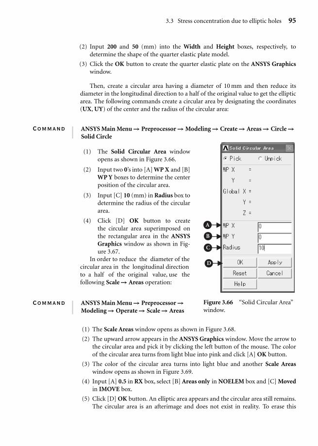
Ch03-H6875.tex 24/11/2006 17: 2 page 95


(2) Input 200 and 50 (mm) into the Width and Height boxes, respectively, todetermine the shape of the quarter elastic plate model.

(3) Click the OK button to create the quarter elastic plate on the ANSYS Graphicswindow.

Then, create a circular area having a diameter of 10 mm and then reduce itsdiameter in the longitudinal direction to a half of the original value to get the ellipticarea. The following commands create a circular area by designating the coordinates(UX, UY) of the center and the radius of the circular area:

Command

A

B

C

D

Figure 3.66 “Solid Circular Area”window.

ANSYS Main Menu → Preprocessor → Modeling → Create → Areas → Circle →Solid Circle

(1) The Solid Circular Area windowopens as shown in Figure 3.66.

(2) Input two 0’s into [A] WP X and [B]WP Y boxes to determine the centerposition of the circular area.

(3) Input [C] 10 (mm) in Radius box todetermine the radius of the circulararea.

(4) Click [D] OK button to createthe circular area superimposed onthe rectangular area in the ANSYSGraphics window as shown in Fig-ure 3.67.

In order to reduce the diameter of thecircular area in the longitudinal directionto a half of the original value, use thefollowing Scale → Areas operation:

Command ANSYS Main Menu → Preprocessor →Modeling → Operate → Scale → Areas

(1) The Scale Areas window opens as shown in Figure 3.68.

(2) The upward arrow appears in the ANSYS Graphics window. Move the arrow tothe circular area and pick it by clicking the left button of the mouse. The colorof the circular area turns from light blue into pink and click [A] OK button.

(3) The color of the circular area turns into light blue and another Scale Areaswindow opens as shown in Figure 3.69.

(4) Input [A] 0.5 in RX box, select [B] Areas only in NOELEM box and [C] Movedin IMOVE box.

(5) Click [D] OK button. An elliptic area appears and the circular area still remains.The circular area is an afterimage and does not exist in reality. To erase this

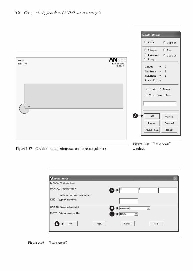
Ch03-H6875.tex 24/11/2006 17: 2 page 96


Figure 3.67 Circular area superimposed on the rectangular area.

A

Figure 3.68 “Scale Areas”

window.

A

B

C

D

Figure 3.69 “Scale Areas”.

Ch03-H6875.tex 24/11/2006 17: 2 page 97


after-image, perform the following commands:

Command ANSYS Utility Menu → Plot → Replot

The circular area vanishes. Subtract the elliptic area from the rectangular area in asimilar manner as described in Section A3.2, i.e.,

Command ANSYS Main Menu → Preprocessor → Modeling → Operate → Booleans →Subtract → Areas

(1) Pick the rectangular area by the upward arrow and confirm that the color of thearea picked turns from light blue into pink. Click the OK button.

(2) Pick the elliptic area by the upward arrow and confirm that the color of the ellipticarea picked turns from light blue into pink. Click the OK button to subtract theelliptic area from the rectangular area to get a quarter model of a plate with anelliptic hole in its center as shown in Figure 3.70.

Figure 3.70 Quarter model of a plate with an elliptic hole in its center created by subtracting an ellipticarea from a rectangular area.

3.3.3.2 INPUT OF THE ELASTIC PROPERTIES OF THE PLATE MATERIAL


(1) The Define Material Model Behavior window opens.

(2) Double-click Structural, Linear, Elastic, and Isotropic buttons one after another.

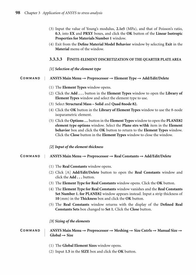
Ch03-H6875.tex 24/11/2006 17: 2 page 98


(3) Input the value of Young’s modulus, 2.1e5 (MPa), and that of Poisson’s ratio,0.3, into EX and PRXY boxes, and click the OK button of the Linear IsotropicProperties for Materials Number 1 window.

(4) Exit from the Define Material Model Behavior window by selecting Exit in theMaterial menu of the window.

3.3.3.3 FINITE-ELEMENT DISCRETIZATION OF THE QUARTER PLATE AREA


Command ANSYS Main Menu → Preprocessor → Element Type → Add/Edit/Delete

(1) The Element Types window opens.

(2) Click the Add . . . button in the Element Types window to open the Library ofElement Types window and select the element type to use.

(3) Select Structural Mass – Solid and Quad 8node 82.

(4) Click the OK button in the Library of Element Types window to use the 8-nodeisoparametric element.

(5) Click the Options … button in the Element Types window to open the PLANE82element type options window. Select the Plane strs w/thk item in the Elementbehavior box and click the OK button to return to the Element Types window.Click the Close button in the Element Types window to close the window.


Command ANSYS Main Menu → Preprocessor → Real Constants → Add/Edit/Delete

(1) The Real Constants window opens.

(2) Click [A] Add/Edit/Delete button to open the Real Constants window andclick the Add . . . button.

(3) The Element Type for Real Constants window opens. Click the OK button.

(4) The Element Type for Real Constants window vanishes and the Real ConstantsSet Number 1. for PLANE82 window appears instead. Input a strip thickness of10 (mm) in the Thickness box and click the OK button.

(5) The Real Constants window returns with the display of the Defined RealConstants Sets box changed to Set 1. Click the Close button.


Command ANSYS Main Menu → Preprocessor → Meshing → Size Cntrls → Manual Size →Global → Size

(1) The Global Element Sizes window opens.

(2) Input 1.5 in the SIZE box and click the OK button.

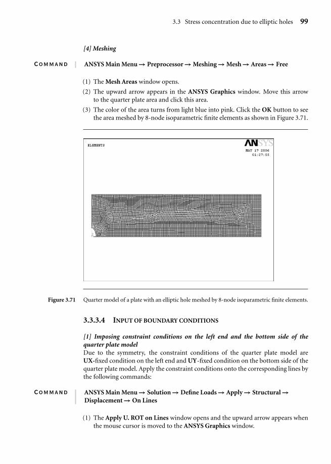
Ch03-H6875.tex 24/11/2006 17: 2 page 99


[4] Meshing

Command ANSYS Main Menu → Preprocessor → Meshing → Mesh → Areas → Free

(1) The Mesh Areas window opens.

(2) The upward arrow appears in the ANSYS Graphics window. Move this arrowto the quarter plate area and click this area.

(3) The color of the area turns from light blue into pink. Click the OK button to seethe area meshed by 8-node isoparametric finite elements as shown in Figure 3.71.

Figure 3.71 Quarter model of a plate with an elliptic hole meshed by 8-node isoparametric finite elements.


[1] Imposing constraint conditions on the left end and the bottom side of thequarter plate modelDue to the symmetry, the constraint conditions of the quarter plate model areUX-fixed condition on the left end and UY-fixed condition on the bottom side of thequarter plate model. Apply the constraint conditions onto the corresponding lines bythe following commands:

Command ANSYS Main Menu → Solution → Define Loads → Apply → Structural →Displacement → On Lines

(1) The Apply U. ROT on Lines window opens and the upward arrow appears whenthe mouse cursor is moved to the ANSYS Graphics window.

Ch03-H6875.tex 24/11/2006 17: 2 page 100


(2) Confirming that the Pick and Single buttons are selected, move the upwardarrow onto the left-end side of the quarter plate area and click the left button ofthe mouse.

(3) Click the OK button in the Apply U. ROT on Lines window to display anotherApply U. ROT on Lines window.

(4) Select UX in the Lab2 box and click the OK button in the Apply U. ROT on Lineswindow.

Repeat the commands and operations (1) through (3) above for the bottom sideof the model. Then, select UY in the Lab2 box and click the OK button in the ApplyU. ROT on Lines window.

[2] Imposing a uniform longitudinal stress on the right end of thequarter plate modelA uniform longitudinal stress can be defined by pressure on the right-end side of theplate model as described below:

Command ANSYS Main Menu → Solution → Define Loads → Apply → Structural →Pressure → On Lines

(1) The Apply PRES on Lines window opens and the upward arrow appears whenthe mouse cursor is moved to the ANSYS Graphics window.

(2) Confirming that the Pick and Single buttons are selected, move the upward arrowonto the right-end side of the quarter plate area and click the left button of themouse.

(3) Another Apply PRES on Lines window opens. Select Constant value in the [SFL]Apply PRES on lines as a box and input −10 (MPa) in the VALUE Load PRESvalue box and leave a blank in the Value box.

(4) Click the OK button in the window to define a uniform tensile stress of 10 MPaapplied to the right end of the quarter plate model.

Figure 3.72 illustrates the boundary conditions applied to the center notched platemodel by the above operations.



(1) The Solve Current Load Step and /STATUS Command windows appear.

(2) Click the OK button in the Solve Current Load Step window to begin the solutionof the current load step.

(3) Select the File button in /STATUS Command window to open the submenu andselect the Close button to close the /STATUS Command window.

(4) When the solution is completed, the Note window appears. Click the Close buttonto close the Note window.

Download - Ansys text book

Top Related