
1
A Markov Test for Alpha
Dean P. Foster, Robert Stine, and H. Peyton Young
September 8, 2011
Abstract. Alpha is the amount by which the returns from a given asset exceed the
returns from the wider market. The standard way of estimating alpha is to
correct for correlation with the market by regressing the asset’s returns against
the market returns over an extended period of time and then apply the t‐test to
the intercept. The difficulty is that the residuals often fail to satisfy
independence and normality; in fact, portfolio managers may have an incentive
to employ strategies whose residuals depart by design from independence and
normality. To address these problems we propose a robust test for alpha based
on the Markov inequality. Since it based on the compound value of the estimated
excess returns, we call it the compound alpha test (CAT). Unlike the t‐test, our test
places no restrictions of returns while retaining substantial statistical power. The
method is illustrated on the distribution for three assets: a stock, a hedge fund,
and a fabricated fund that is deliberately designed to fool standard tests of
significance.

2
1. Testing for alpha
An asset that consistently delivers higher returns than a broad‐based market
portfolio is said to have positive alpha. Alpha is the mean excess return that results
from the asset manager’s superior skill in exploiting arbitrage opportunities and
judging the risks and rewards associated with various investments. How can
investors (and statisticians) tell from historical data whether a given asset
actually is generating positive alpha relative to the market? To answer this
question one must address four issues: i) multiplicity; ii) trends; iii) cross‐
sectional correlation; iv) robustness. We begin by reviewing standard
adjustments for the first three; this will set the stage for our approach to the
robustness issue, which involves a novel application of the Markov inequality.
The first step in evaluating the historical performance of a financial asset requires
adjusting for multiplicity. Assets are seldom considered in isolation: investors
can choose among hundreds or thousands of stocks, bonds, mutual funds, hedge
funds, and other financial products. Without adjusting for multiplicity, statistical
tests of significance can be seriously misleading. To take a trivial example, if we
were to test individually whether each of 100 mutual funds “beats the market” at
level p = 0.05, we would expect to find five statistically significant p‐values when
in fact none of them beats the market.
The literature on multiple comparisons includes a wide variety of procedures to
correct for multiplicity. The simplest and most easily used of these is the
Bonferroni rule. When testing m hypotheses simultaneously, one compares the
3
observed p‐values to an appropriately reduced threshold. For example, instead of
comparing each p‐value ip to a threshold such as p = 0.05, one would compare
them to the reduced threshold p /m.
Modern alternatives to Bonferroni have extended it in two directions. The first,
called alpha spending, allows the splitting of the alpha into uneven pieces; see
for example Pocock (1977) and OʹBrien and Fleming (1979). The second group of
extensions provides more power when several different hypotheses are being
tested. These can be motivated from many perspectives: false discovery rate
(Benjamini and Hochberg 1995), Bayesian (George and Foster, 2000), information
theory (Stine, 2004) and frequentist risk (Abramovich, Benjamini, Donoho, and
Johnstone, 2006). One can even apply several of these approaches
simultaneously (Foster and Stine, 2007). In the case of financial markets,
however, the natural null hypothesis is that no asset can beat the market for an
extended period of time because this would create exploitable arbitrage
opportunities. Thus, in this setting, the key issue is whether anything beats the
market, let alone whether multiple assets beat the market.
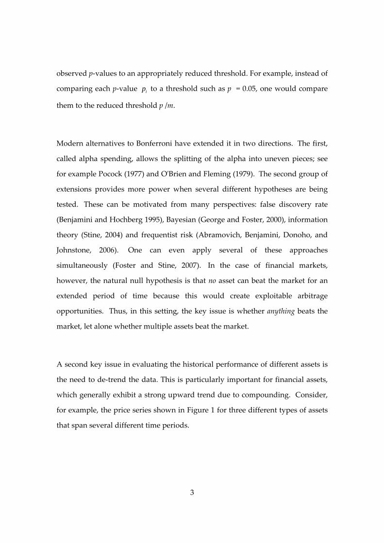
A second key issue in evaluating the historical performance of different assets is
the need to de‐trend the data. This is particularly important for financial assets,
which generally exhibit a strong upward trend due to compounding. Consider,
for example, the price series shown in Figure 1 for three different types of assets
that span several different time periods.
4
Figure 1. Value of three assets observed monthly over different time periods.
Berkshire Hathaway is a stock that is famous for its superior performance over a
long period of time. TEAM is a fund that is based on a dynamic rebalancing
algorithm which seeks to reduce volatility while maintaining high returns
(Gerth, 1999; see also Agnew, 2002). This fund is especially interesting because
(unlike many other hedge funds) its rebalancing strategy is explicit and its
holdings are transparent: one knows at all times what assets are contained in the
portfolio. By contrast the Piggyback Fund is assumed to be entirely
nontransparent (to its investors). The reason is that it is based on an options
trading strategy that is designed to fool investors into believing that the fund
manager is able to ’beat the market’ when in fact he is manufacturing high
current returns by hiding large potential losses in the tail of the distribution (Lo,
2001; Foster and Young, 2010).
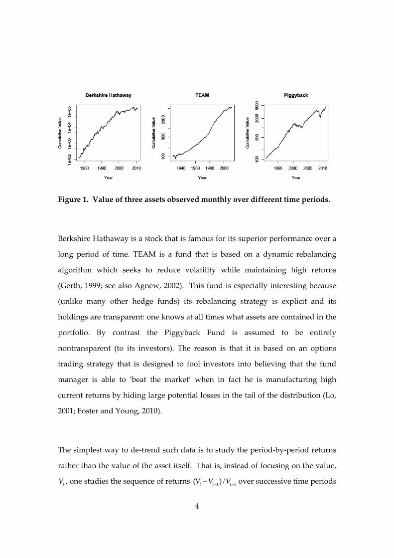
The simplest way to de‐trend such data is to study the period‐by‐period returns
rather than the value of the asset itself. That is, instead of focusing on the value,
tV , one studies the sequence of returns 1 1( ) /t t tV V V over successive time periods
5
t (see figure 2). The hope is that the returns are being generated by a process that
is sufficiently stationary for standard statistical tests to be applied. As we shall
see, this hope may not be well‐founded given that financial portfolios are often
managed in a way that produces highly nonstationary behavior by design.
The third issue, cross‐sectional correlation, arises because returns on financial
assets often exhibit a high degree of positive correlation. The standard way to
deal with this problem is the Capital Asset Pricing Model (CAPM), which
partitions the variation in asset returns into two orthogonal components: market
risk, which is non‐diversifiable and hence unavoidable, and idiosyncratic risk.
By construction, idiosyncratic risk is orthogonal to market risk and measures the
rewards and risks associated with a specific asset. It is the mean return on this
idiosyncratic risk, known as alpha, that draws investors to specific stocks, mutual
funds, and alternative investment vehicles such as hedge funds.
Figure 2. Monthly returns series for the three assets
The standard way to estimate the alpha of a particular asset or portfolio of assets
such as a mutual fund is to regress its returns against the returns from a broad‐

6
based market index such as the S&P 500 after subtracting out the risk‐free return.
Specifically, let the random variable tM denote the return generated by the
market portfolio in period t , and let tr be the risk‐free rate of return during the
period, that is, the return available on a safe asset such as US Treasury Bills. The
excess return of the market during the tht period is t tM r . Let itY denote the
return in period t from a particular asset (or portfolio of assets) identified by the
superscript i. The portfolio’s excess return is defined as it tY r . CAPM posits that
the excess return on each asset in the tth period is a multiple of the excess return
on the market plus a random term it that has mean zero and is uncorrelated
with the market excess returns, that is,
( ) i i it t t t t tY r M r , (1)
where [ ] 0 itE and [ ( )] 0 i
t t tE M r .
The coefficient ti is the beta of the asset. Beta describes how returns on the asset
co‐vary with returns on the market as a whole, while it is the idiosyncratic risk
associated with the asset. A portfolio that leverages stocks has beta larger than
1, whereas a portfolio of bonds has beta approaching 0. Typically beta will vary
over time as the portfolio manager changes his level of exposure to the market.
Let the random variable tY denote the return on a specific asset in time period t,
where we drop the superscript i. The returns on the asset beat the market if in
expectation it is positive. If this is the case, an investor could increase his
overall return by investing a portion of his wealth in this asset instead of in the
market. Moreover, this increased return could be achieved without exposing

7
himself to much additional volatility, provided he puts a sufficiently small
proportion of his wealth in the asset.
A second way in which an actively managed asset (such as a mutual fund) can
beat the market is through market timing. Suppose that the manager invests a
proportion pt of its total wealth in the market at time t and leaves the rest in cash
earning the risk-free rate tr . The manager can adjust pt depending on his belief
about future market movements. If he expects the market to rise he might buy
shares on margin, which corresponds to pt 1 and t > 1. If the manager
expects the market to fall, he can short the market which implies that 0tp and
t < 0. A portfolio manager who successfully anticipates market movements is
just as attractive as a manager who invests in assets which intrinsically have
positive alpha. The asset labeled TEAM in figures 1 and 2 is an example of an
actively managed portfolio in which the relative proportions allocated to cash
and the market are rebalanced at the end of each period.
The standard way of estimating alpha is first to estimate the manager’s level of
exposure to the market at each point in time ( it ), and then to compute the mean
of the residuals 1
(1 / )
it
t T
T as defined in (1). However, this fails to take
successful market timing into account, which can be just as valuable as choosing
specific investments. We therefore propose a generalization of alpha that
incorporates skill in market timing as well as skill in choosing superior
investments.

8
This concept is defined as follows. Given returns data for periods t = 1, …, T, let
, t t t t t tM M r Y Y r . (2)
Compute the means 1
(1/ ) tt T
M T M
and 1
(1/ ) tt T
Y T Y
, and let
1
2
1
( )( )
( )
t tt T
tt T
Y Y M M
M M
. (3)
Thus is the coefficient in the OLS regression of Y on tM over the entire
observation period. 1 We can then formally rewrite (1) as follows:
t t tY M A , where t t t tA M . (4)
The random variable tA represents generalized alpha, which includes the returns
from market timing and excess returns from the specific assets in the portfolio.
The standard way of conducting a test of significance would be to apply the t‐test
to the intercept in the regression specified in (4). However, the t‐test presumes
that the residuals tA satisfy independence and normality, and there is no
particular reason to think that these conditions hold in the present case. Indeed,
when we graph the residuals from our three candidate assets over time, it
1 We remark that can also be interpreted as a weighted average of the period‐by‐period values
t , weighted by the relative volatility of the asset in each period.
9
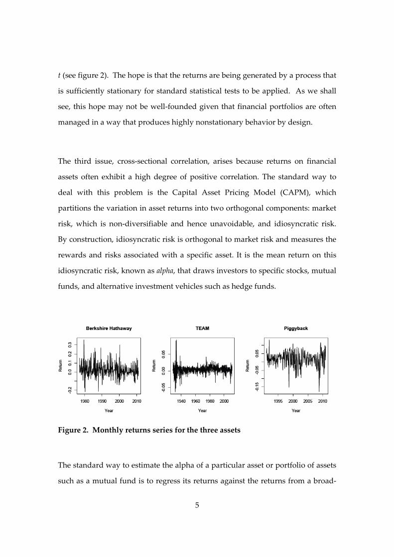
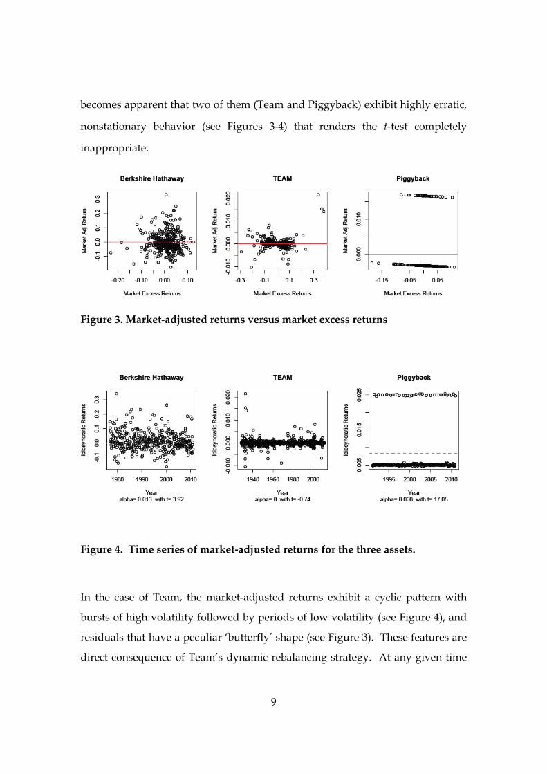
becomes apparent that two of them (Team and Piggyback) exhibit highly erratic,
nonstationary behavior (see Figures 3‐4) that renders the t‐test completely
inappropriate.
Figure 3. Market‐adjusted returns versus market excess returns
Figure 4. Time series of market‐adjusted returns for the three assets.
In the case of Team, the market-adjusted returns exhibit a cyclic pattern with
bursts of high volatility followed by periods of low volatility (see Figure 4), and
residuals that have a peculiar ‘butterfly’ shape (see Figure 3). These features are
direct consequence of Team’s dynamic rebalancing strategy. At any given time
10
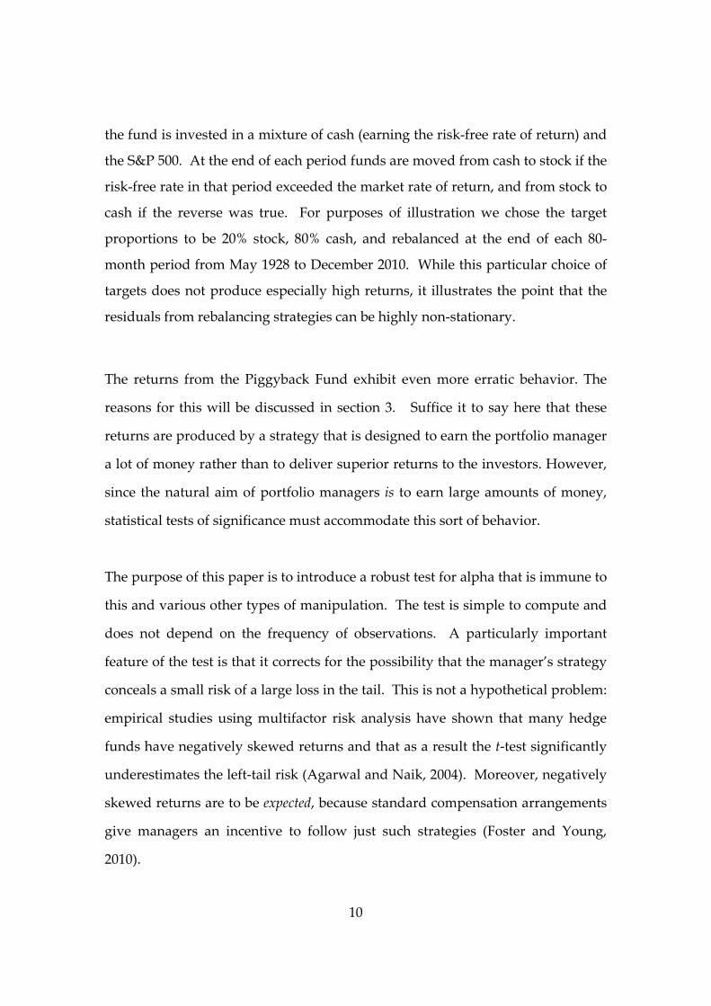
the fund is invested in a mixture of cash (earning the risk-free rate of return) and
the S&P 500. At the end of each period funds are moved from cash to stock if the
risk-free rate in that period exceeded the market rate of return, and from stock to
cash if the reverse was true. For purposes of illustration we chose the target
proportions to be 20% stock, 80% cash, and rebalanced at the end of each 80-
month period from May 1928 to December 2010. While this particular choice of
targets does not produce especially high returns, it illustrates the point that the
residuals from rebalancing strategies can be highly non-stationary.
The returns from the Piggyback Fund exhibit even more erratic behavior. The
reasons for this will be discussed in section 3. Suffice it to say here that these
returns are produced by a strategy that is designed to earn the portfolio manager
a lot of money rather than to deliver superior returns to the investors. However,
since the natural aim of portfolio managers is to earn large amounts of money,
statistical tests of significance must accommodate this sort of behavior.
The purpose of this paper is to introduce a robust test for alpha that is immune to
this and various other types of manipulation. The test is simple to compute and
does not depend on the frequency of observations. A particularly important
feature of the test is that it corrects for the possibility that the manager’s strategy
conceals a small risk of a large loss in the tail. This is not a hypothetical problem:
empirical studies using multifactor risk analysis have shown that many hedge
funds have negatively skewed returns and that as a result the t‐test significantly
underestimates the left‐tail risk (Agarwal and Naik, 2004). Moreover, negatively
skewed returns are to be expected, because standard compensation arrangements
give managers an incentive to follow just such strategies (Foster and Young,
2010).

11
The plan of the paper is as follows. In section 2 we derive our test in its most
basic form. The essential idea is to adjust the returns by first subtracting off the
risk‐free rate, then correcting for overall correlation with the market as in (3‐4),
and then compounding the residuals. We then apply the Markov inequality to
test whether the compound value is growing, i.e. whether the final value is larger
than the initial value with a high degree of confidence.
Section 3 shows why it is vital to have a test that is robust against erratic and
nonstationary behavior of the residuals. In particular, we show that the t‐test
applied to the residuals leads to a false degree of confidence in the Piggyback
Fund, which is constructed so that it looks like it produces positive alpha when
this is not actually the case. In a second example we show why some other
nonparametric tests, such as the martingale maximal inequality, are also
inappropriate in this setting. The difficulty is that the fund manager can
manipulate the degree of correlation with the market so that the overall degree of
correlation is low, but in some periods the correlation is high. Thus the end value
of the fund may not be impressive even though its interim value is large. This
type of manipulation does not fool the Markov test, which is applied only to the
final value of the fund, but it can fool the martingale maximal inequality, which
is based on the maximum value achieved over the period.
In section 4 we show how to boost the statistical power of the test by leveraging
the asset. First we show that if the returns of the asset are lognormally
distributed with known variance, then we can choose a level of leverage such
that the loss in power is quite low relative to the optimal test, which in this case

12
is the t‐test. In fact, for a p‐value of .01 the loss in power is less than 30%, and for
a p‐value of .001 the loss in power is only about 20%. We then show how to
extend this approach to situations where we do not know the mean or variance
of the asset in question. In this case we create a hypothetical composite portfolio
such that each asset in the portfolio represents a different level of leverage
applied to the original asset. We invest equal amounts in each of these
hypothetical assets at the start of the observation period, compute the maximum
final value of the portfolio at the end of the period, and apply our Markov test at
a given level of significance. It can be shown that this leveraged version of the
test is asymptotically as powerful as the optimal test when the returns are
lognormally distributed, which is the standard assumption for many financial
assets.
In section 5 we illustrate how our approach can be applied to data, focusing on
the particular case of Berkshire. First we derive the market‐adjusted monthly
returns by subtracting off the risk‐free rate and correcting for correlation with the
market. Then we apply different amounts of leverage to these returns, taking
into account the costs associated with higher levels of leverage (because of the
need to insure that the fund does not go bankrupt in any given period). The
resulting Berkshire p‐value is quite impressive – about 0.00095.
We need to consider, however, that we chose this stock precisely because it has
been a stellar performer over a long period of time. If Berkshire is the best out of
a population of 500 stocks, for example, then the Bonferroni correction would
imply that the appropriate p‐value is (0.00095)500 = 0.475, which is not
significant. In other words, Berkshire considered by itself is very impressive, but
out of a large population of stocks it is much less so.

13
2. The compound alpha test (CAT)
Consider a financial asset, such as a stock, a mutual fund, or a hedge fund whose
performance we wish to compare with that of the market. The data consist of
returns generated by the asset over a series of reporting periods 1,2,...,t T .
Denote the market return in period t by the random variable tM and the asset’s
return by the random variable Y . In applications, tM would be the return on a
broad‐based portfolio of stocks such as the S&P 500 or the Wilshire 5000.
The first step in the analysis is to subtract off the risk‐free rate of return in each
period, that is, the rate available on a safe asset such as Treasury bills. In other
words we define the random variables t t tM M r and t t tY Y r , where tr
denotes the risk‐free rate in period t. The second step is to correct for correlation
with the market over the entire period, that is, we compute the slope from the
OLS regression of Yt on Mt as in (3). We then define the market‐adjusted return in
period t as follows
t t tA Y M . (5)
Next we truncate the returns so that the total return 1 tA in each period is
nonnegative. If the prices of tY and tM evolve in continuous time with no jumps,
this can be achieved by placing a stop‐loss order on the market‐adjusted asset
t t tA Y M . In this case the truncated total return is simply [1 ] tA .

14
An alternative approach is to insure the asset for the duration of the period using
options. Assuming that 0 , one buys a call option on the market that limits
the risk from a large positive realization of tM , and a put option on the asset that
limits the risk of a large negative realization of tY . A crucial point is that, for
ordinary financial assets such as publicly traded stocks and mutual funds, the
cost of such insurance is very small when the time periods are short. (The
reason is that the variance in returns of most assets scales in proportion to the
length of the period.) Thus if the length of each period is sufficiently small, the
probability that the returns will exceed a specified threshold is small, which
implies that the price of insuring against such an event is small.2
To illustrate, suppose that 0.5 and that the length of each period is one
month. One can buy a call that protects against a rise of 67% or more in the
market by the end of the month, and a put that protects against a fall of more
than 67% in the price of the asset. This will guarantee that the market‐adjusted
asset cannot lose more than 100% of its value during the period, i.e., that 1 tA is
nonnegative.3 The cost of such insurance will typically be very small because the
probability of such an extreme move in one month’s time is very remote;
moreover it will be even more remote if we take the duration of the options to be
even shorter, say one week. (In section 5 we estimate the monthly cost of
insuring Berkshire Hathaway in this manner using empirical data on options
prices.)
2 For further details on options pricing see Hull (2009) or Campbell, Lo, and MacKinlay (1997). 3 The relative amount of protection in puts and calls can be chosen in many different ways to
protect against a 100% drop in the market‐adjusted asset. One would choose the cheapest such
mixture based on the prices of the options.

15
Let be the length of each period, and let ( )t tc c represent the cost of
insuring against negative realizations of the market‐adjusted return 1 tA in
period t. That is, at the start of the period we spend the fraction / (1 )t tc c of the
portfolio on insuring the remainder of the portfolio (1/ (1 )tc ) against
bankruptcy by the end of the period. Thus the total return (net of insurance
costs) is given by the nonnegative random variable
[1 ] / (1 ) t t tB A c . (6)
(For notational convenience we omit the dependence on .) Consider the
compound value of the 'tB s over the T periods of observation:
1
T tt T
C B . (7)
The null hypothesis is that [ ] 0TE C . Since tB is a nonnegative random variable,
the Markov inequality implies that this hypothesis can be rejected at significance
level p if 1 /TC p .
Compound Alpha Test (CAT). Let TC be the compound market‐adjusted return of a
candidate asset through period T. The null hypothesis that the asset does not have
positive alpha. This hypothesis can be rejected at significance level p if
1 /TC p . (8)
16
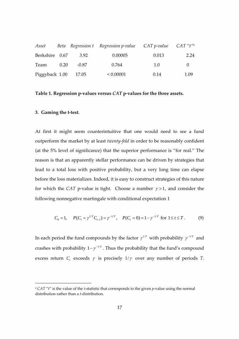
Note that the compound value TC must be very large before CAT rejects the null
at a standard level of significance. For example, to reject the null at the 5% level
of significance requires that the asset grow by twenty‐fold after subtracting off the
risk‐free rate and correcting for correlation with the market.
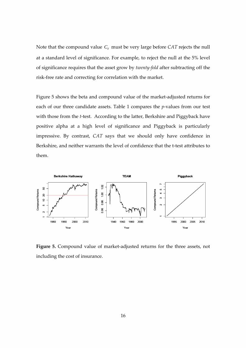
Figure 5 shows the beta and compound value of the market‐adjusted returns for
each of our three candidate assets. Table 1 compares the p‐values from our test
with those from the t‐test. According to the latter, Berkshire and Piggyback have
positive alpha at a high level of significance and Piggyback is particularly
impressive. By contrast, CAT says that we should only have confidence in
Berkshire, and neither warrants the level of confidence that the t‐test attributes to
them.
Figure 5. Compound value of market‐adjusted returns for the three assets, not
including the cost of insurance.
17
Asset Beta Regression t Regression p‐value CAT p‐value CAT “t”4
Berkshire 0.67 3.92 0.00005 0.013 2.24
Team 0.20 ‐0.87 0.764 1.0 0
Piggyback 1.00 17.05 < 0.00001 0.14 1.09
Table 1. Regression p‐values versus CAT p‐values for the three assets.
3. Gaming the t‐test.
At first it might seem counterintuitive that one would need to see a fund
outperform the market by at least twenty‐fold in order to be reasonably confident
(at the 5% level of significance) that the superior performance is “for real.” The
reason is that an apparently stellar performance can be driven by strategies that
lead to a total loss with positive probability, but a very long time can elapse
before the loss materializes. Indeed, it is easy to construct strategies of this nature
for which the CAT p‐value is tight. Choose a number 1 , and consider the
following nonnegative martingale with conditional expectation 1
0 1,C 1/ 1/1( ) ,T T
t tP C C 1/( 0) 1 T
tP C for 1 t T . (9)
In each period the fund compounds by the factor 1/T with probability 1/T and
crashes with probability 1/1 T . Thus the probability that the fund’s compound
excess return tC exceeds is precisely 1/ over any number of periods T.
4 CAT “t” is the value of the t‐statistic that corresponds to the given p‐value using the normal
distribution rather than a t‐distribution.

18
Returns series with this property can be constructed using standard options
contracts (Foster and Young, 2010).
The Piggyback Fund is constructed along just these lines. Namely, the fund is
invested in the S&P 500, and the returns are reported every month. However,
once every six months the total return is artificially boosted by the factor 1.02.
This can be done by taking an options position in the S&P 500 that bankrupts the
fund if the options are exercised. The strike price is chosen so that the probability
of this event is 1/1.02 = .9804, so the fair value of the option is zero. With
probability 1/1.02 the fund grows by the factor 1.02 and with probability .02/1.02
it loses everything, which is a lottery with expectation zero. This strategy
explains the bizarre pattern of the market‐adjusted residuals in Figure 3: one‐
sixth of the time they are + 2%, and five‐sixths of the time they are –2%. With less
than 25 years of data there is a sizable probability that the downside risk will
never be realized, and investors will be lulled into thinking that the fund is
generating positive alpha. Because it guards against this possibly unobserved
volatility, CAT attaches a modest p‐value to the returns generated by the
Piggyback Fund.
Of course, even a casual inspection of the residuals in Figures 3‐4 suggests that
the t‐test should not be used in this case. However this is not the essence of the
problem, because it is easy to construct similar strategies whose returns look i.i.d.
normal. For instance, suppose that every month the manager boosts the fund’s
returns by the factor 1.0033 where is a lognormally distributed error with
mean 1 and small variance. (The purpose of the variation is to lend plausible
variability to the realized returns.) As before, the boost comes at the cost of
19
going bankrupt with probability 1/(1.0033 ) .9967 / each month. Assuming
that the variance of is small, this scheme will run for about 300 months (25
years) before the fund goes bankrupt, and the residuals will look very
convincing. Thus, in this case the t‐test would seem to be appropriate, and the
estimate of alpha will be about 4% per year at a very high level of significance.
This is misleading, however, because in reality the distribution of returns is not
approximately normal ‐‐ there is a large potential loss hidden in the tail. One of
the main virtues of our test is that it corrects for this “hidden volatility”: after 25
years the p‐value of this scheme will only be about 300(1.0033) .37p .
A different manipulation based on market timing requires that CAT rely on the
final cumulative return after a fixed test period rather than, say, using the
maximum return over t = 1,…,T. The idea of this manipulation is to disguise a
highly leveraged market position as an asset whose overall = 0. For instance,
one can obtain such an asset by leveraging the market to obtain the returns
2 t tY M for t = 1,…,T/2. For the remainder of the test period, one would short
the market so that the returns are 2 t tY M for t = T/2,…,T. By construction,
= 0 and t tA Y . Given the generally positive returns produced by the US stock
market, the intermediate cumulative return is very likely to exceed an impressive
threshold.
To illustrate, Figure 6 tracks the compounded monthly returns from a fund that
leveraged the market by a factor of 2 from January 1926 to June 1968, then
leveraged it by a factor of ‐2 from July 1968 to December 2010. By mid‐1968 the
fund’s value has grown by a factor of 226. If the null hypothesis is that the
market‐adjusted returns form a martingale, then by the martingale maximal
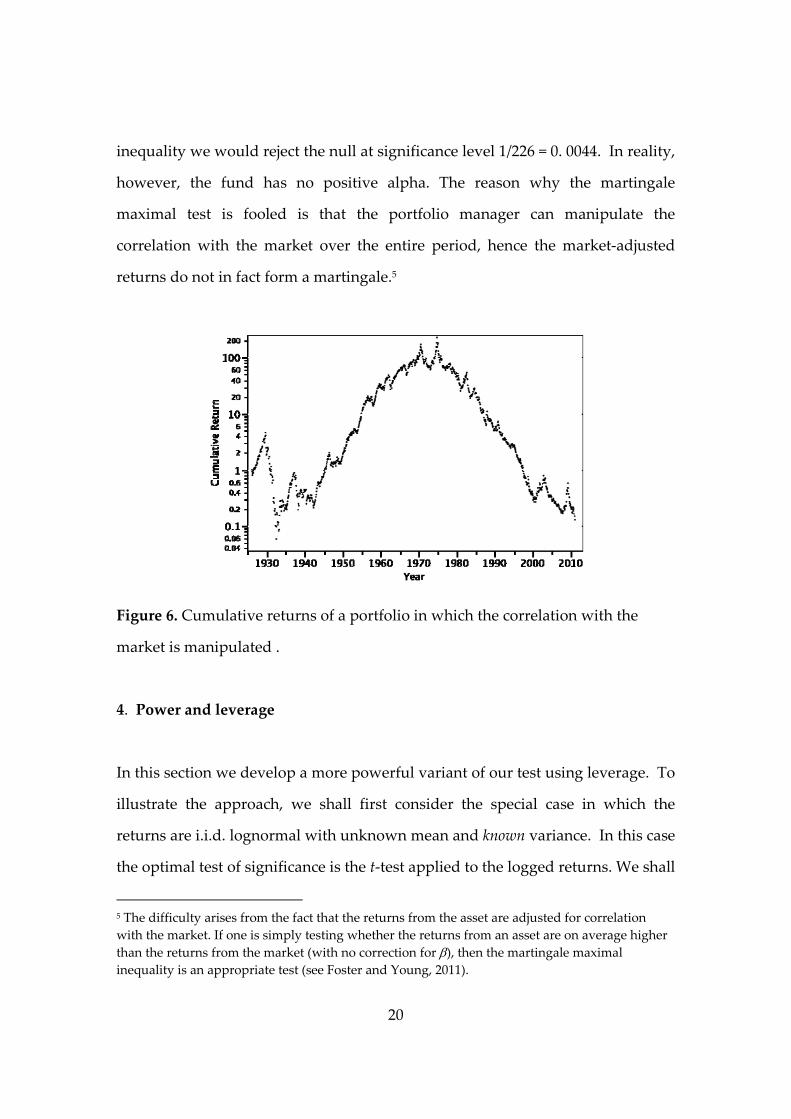
20
inequality we would reject the null at significance level 1/226 = 0. 0044. In reality,
however, the fund has no positive alpha. The reason why the martingale
maximal test is fooled is that the portfolio manager can manipulate the
correlation with the market over the entire period, hence the market‐adjusted
returns do not in fact form a martingale.5
Figure 6. Cumulative returns of a portfolio in which the correlation with the
market is manipulated .
4. Power and leverage
In this section we develop a more powerful variant of our test using leverage. To
illustrate the approach, we shall first consider the special case in which the
returns are i.i.d. lognormal with unknown mean and known variance. In this case
the optimal test of significance is the t‐test applied to the logged returns. We shall
5 The difficulty arises from the fact that the returns from the asset are adjusted for correlation
with the market. If one is simply testing whether the returns from an asset are on average higher
than the returns from the market (with no correction for ), then the martingale maximal
inequality is an appropriate test (see Foster and Young, 2011).
21
show that by leveraging the asset at an appropriate level (which is determined by
the variance), we obtain a generalization of our test that involves only a modest
loss of power compared to the optimal test. Then we shall show that a similar
result holds even when we do not know the variance.
To be concrete, consider a manager whose fund is generating compound returns
CT 0 relative to the risk‐free rate and suppose for simplicity that there is no
correlation with the market ( 0) . Let us further assume that CT is
lognormally distributed:
ln TC ~ 2 2(( / 2) , ) N T T . (10)
This is consistent with the traditional representation of asset returns as a
geometric Brownian motion in continuous time, that is, a stochastic differential
equation of form t t t tdC C dt C dW (Berndt, 1996; Campbell, Lo, and
MacKinlay, 1997). When the asset is leveraged by the factor 0 ,6 the log of the
compound returns at time T, CT() , are normally distributed:
ln ( )TC ~ 2 2 2 2(( / 2) , ) N T T . (11)
Suppose, for the moment, that 2 is known and is not. The null hypothesis is
that 0 and the alternative hypothesis is that 0 . Choose a level of
6 To leverage an asset which sells for $1 by the factor one borrows ‐1 dollars at the risk‐free rate and invests dollars in the asset. If < 1 this means that – is invested in the risk‐free asset and the remainder in the risky asset. Notice that to keep a constant level of leverage at all times
one needs to rebalance the absolute amounts invested in each asset. In continuous time this yields
the process t t t t
dC C dt C dW .

22
significance 0p and a time T at which a test of significance is to be conducted.
CAT rejects the null at level p if and only if
logCT() log(1 / p) . (12)
Under the null hypothesis,
Z
T
logCT() (2 2 / 2)T
T is (0,1)N . (13)
Hence CAT rejects the null if and only if
Z
T
log(1 / p) (2 2 / 2)T
T. (14)
To maximize the power of the test we choose the leverage so that the probability
of rejection is maximized. This occurs when the right‐hand side of (14) is
minimized, that is, when
* 2log(1 / p)
T. (15)
Notice that * depends on the variance of the process, the time at which the test
is conducted, and the level of significance p. However, the corresponding z‐
value depends only on p, that is, the test rejects if and only if
ZT 2log(1 / p) c
p. (16)

23
We can interpret pc as the critical value of CAT at significance level p . We wish
to compare this with the critical value of the t‐test, which rejects at level p if and
only if
ZT 1(1 p) z
p. (17)
Let ( )L p denote the maximum power loss at significance level p over all
combinations of , , T . In other words, ( )L p is the maximum probability that
the t‐test rejects the null at level p when our test accepts.
Theorem 1. If CAT is applied to a lognormally distributed asset at significance level p,
the maximum power loss ( )L p is bounded above by 2 (.5( )) 1 p pc z . Moreover
( ) 0L p as 0p .
The proof is given in the Appendix.
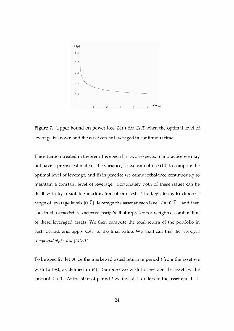
Figure 7 plots the upper bound on the power loss ( )L p as given in the
proposition. Observe that the loss is about 20‐25% for p in the range 310 to 510 .
These p‐values are appropriate when we are testing the best asset out of a large
population of candidate assets. For example, if we are testing whether the best of
100 assets has positive alpha at significance level 0.01, the asset would have to
pass our test at level 0.0001, by the Bonferroni correction.
24
Figure 7. Upper bound on power loss ( )L p for CAT when the optimal level of
leverage is known and the asset can be leveraged in continuous time.
The situation treated in theorem 1 is special in two respects: i) in practice we may
not have a precise estimate of the variance, so we cannot use (14) to compute the
optimal level of leverage, and ii) in practice we cannot rebalance continuously to
maintain a constant level of leverage. Fortunately both of these issues can be
dealt with by a suitable modification of our test. The key idea is to choose a
range of leverage levels [0, ] , leverage the asset at each level [0, ] , and then
construct a hypothetical composite portfolio that represents a weighted combination
of these leveraged assets. We then compute the total return of the portfolio in
each period, and apply CAT to the final value. We shall call this the leveraged
compound alpha test (LCAT).
To be specific, let tA be the market‐adjusted return in period t from the asset we
wish to test, as defined in (4). Suppose we wish to leverage the asset by the
amount 0 . At the start of period t we invest dollars in the asset and 1

25
dollars in the risk‐free asset (i.e., Treasury bills). Note that if 1 this means that
we are borrowing at the risk‐free rate to buy the asset on margin. Given our
assumption that we cannot rebalance in continuous time during the course of the
period, we need to insure against tail risk by purchasing options. In particular,
we need to purchase options that effectively trim off negative realizations of the
leveraged returns 1 tA . This insurance comes at a cost, say ( )tc per dollar
of the asset at the start of the period, where is the length of the period.
Typically the variance in the returns tA scales by the factor , and hence for any
given value of , ( ) 0tc as 0 . (In the next section we shall analyze a
concrete example (Berkshire) in detail, and show that the cost of options
insurance is very small when is on the order of one month .)
Let [0, ] be a range of leverage levels and let ( )f be a density with full support
on [0, ] . The total return on the ‐leveraged asset in period t is given by the
nonnegative random variable
(1 )
( )(1 ( ))
tt
t
AB
c
. (18)
At the start of period t = 1, weight the various leverage levels in [0, ] according
to the distribution ( )f . (Note that ( )f determines the initial weighting; the
relative amounts invested in the various assets will change over time and are not
rebalanced.) The final value of this composite portfolio at the end of period T is
0
1
( ) ( ) ( )T tt T
C f B f d
. (19)
26
The null hypothesis is that [ ] 0tE A for all t T , which implies that [ ( )] 1TE C f .
Note that when is sufficiently small, the options costs are small over the entire
range [0, ] , hence the null hypothesis is essentially equivalent to the statement
[ ( )] 1TE C f . We can therefore reject the null at significance level p if
( ) 1/TC f p . (20)
This is the leveraged compound alpha test (LCAT) with density ( )f . As we have
already noted, this test is robust against a wide variety of manipulations that a
portfolio manager can employ to make the returns look better than they really
are. It is therefore rather surprising to find that the loss in power is actually quite
small. In fact, we claim that LCAT is asymptotically as powerful as the optimal test
when the returns are lognormally distributed and the time periods are short.
Theorem 2. Consider an asset with market‐adjusted returns tA that are lognormally
distributed with unknown mean and variance. Let ( )f be a density with full support
on an open interval (0, ) that contains the optimal level of leverage as defined in (15).
Given any small > 0, the maximum power loss of LCATat significance level p, relative
to the t‐test, is less than when p is sufficiently small and the time intervals are
sufficiently short.
This result is related to the pioneering work of Cover (1991) on ‘universal
portfolios.’ However, our focus is on estimating the power loss of a particular
test relative to the optimal test, which requires a separate proof. The essence of
the argument can be sketched as follows (for details see Foster and Young
(2011)). We already know from theorem 1 that there exists a level of leverage *
27
such that CAT is asymptotically as powerful as the optimal test for small values
of p. In particular, if the t‐test rejects the null hypothesis for this leveraged asset,
then CAT is almost certain to reject it also. This happens if the leveraged asset
has grown by a factor exceeding 1/p. Assets that are leveraged at levels close to
* will grow by nearly the same factor. Therefore, if the composite portfolio
initially puts a positive fraction q > 0 of funds into leverage levels near * , the
final compound value of the portfolio will grow by a factor of about q/p. (In fact
this is an underestimate, because it ignores the growth in value of the assets
outside this small neighborhood). In particular, the null will be rejected at the
level of significance p/q. It can be shown, however, that the probability of
making a type‐I error at level p/q is nearly the same as the probability of making
a type‐I error at level p when p is sufficiently small (and q is fixed). The details
are somewhat involved and we shall not give them here; in particular one must
show that the argument works when the costs of options are taken into account
(see Foster and Young, 2011).7
5. Empirical analysis
In this section we shall apply our framework to the three assets shown in Figures
1‐4, with a particular focus on Berkshire. Let us recapitulate the basic steps in the
test. We are given a candidate asset whose returns are observed over T periods:
1 2, ,..., TY Y Y . Denote the market returns over the same T periods by 1 2, ,..., TM M M ,
where the “market” refers to some broad‐based index such as the S&P 500 or the
7 Foster and Young (2011) use the martingale maximal inequality as a test of excess returns. This
is a more powerful test than the Markov inequality when applied to martingale data. However,
their estimates of power loss are based on the Markov inequality applied to end‐of‐period value
(just as we do here), hence their estimates are valid in the present situation.

28
Wilshire 5000. Denote the risk‐free rates of return by 1 2, ,..., Tr r r .
Step 1. Compute the regression coefficient between the asset’s excess returns
Yt Yt rt and the market’s returns excess returns Mt Mt rt :
1
2
1
( )( )
( )
t tt T
tt T
Y Y M M
M M
.
Step 2. For each t compute the market‐adjusted return
t t tA Y M
Step 3. Choose a range of leverage levels 1 20 ... m . Estimate the cost
( )t kc of insuring the k -leveraged asset against default during period t. For each
t and each value k compute the insured returns
, [1 ] / (1 ( ))t k k t t kB A c .
Step 4. Compute the compound values
,1
k k tt T
C B
and 1
(1/ ) kk m
C m C
.
Step 5. Reject the null hypothesis at level p if 1/C p .

29
How should one choose the range of leverage levels in step 3? One approach is
the following. The expected long-run growth rate of any asset is roughly equal
to its mean return minus one-half of the variance (the volatility drag). (In fact
this statement holds exactly if the returns are lognormally distributed.) This
suggests that to maximize the compound value of the leveraged market-adjusted
returns, one should choose the leverage equal to the mean divided by the
variance of the returns. Since this is only a rough estimate of the optimal
leverage level, we should in fact choose a range of levels on either side of the
estimate.
We shall now illustrate this procedure by analyzing the performance of Berkshire
Hathaway from November 1976 to December 2010.8 The overall beta for the
period is = .67. The mean market-adjusted return [ ]t
A E A is 0.0127 per
month and the variance is 0.000427 per month. Thus we take
0.0127 / 0.00427 3 as a reasonable place to center the range of leverage
levels.
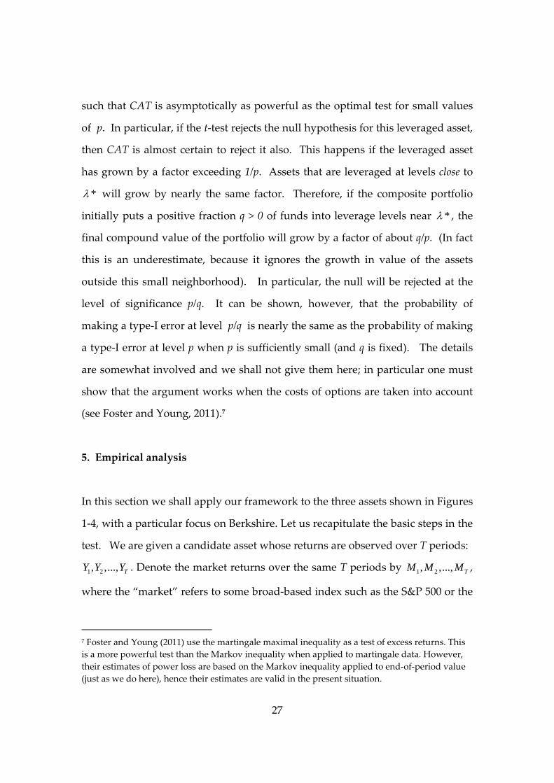
Next we compute the compound value of the market-adjusted leveraged returns
at each of the levels 1,2,3,4,5 but without including options costs. The
growth in these compound values over the period is shown in Figure 8. The
maximal final value in 2010 was 4, 426 (leverage 3). When the five levels are
weighted equally the final value is 1,834C .
8 A similar analysis can be applied to Team but it turns out that leveraging does little to increase
the compound returns over the observation period. The analysis cannot be applied to the
Piggyback Fund because there is no way to insure the returns, hence the fund cannot be
leveraged.
30
Figure 8. Compound value of market-adjusted returns on Berkshire Hathaway,
leveraged at five different levels over the period Nov 1976 - Dec 2010.
The reciprocal of the value C gives us a preliminary estimate of the level of
significance (in this case 1 / 0.00054C ). If the result is not significant we need
proceed no further. If it is significant, however, we need to refine the analysis by
including the cost of insuring that the returns stay non-negative. For example, to
protect the market-adjusted return .67t t tA Y M for one month leveraged five
times, one could buy five puts on Berkshire and five calls on the market that
expire in 30 days. The strike prices need to be chosen to protect against a decline
of more than 20% in the value of tA . This will be true if the puts protect against
a fall of more than x% in Berkshire and the calls protect against a rise of more
than y% in the market, where x + .67y = 20. The least costly combination
depends on the relative volatility of Berkshire versus the market, where the latter
is taken to be the S & P 500.
31
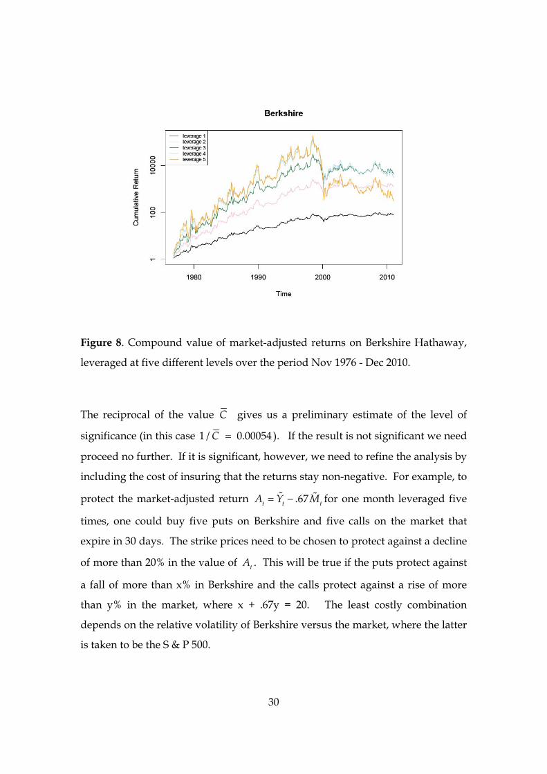
Using data on options prices in May 2011, we estimated the cost of insuring
Berkshire at five different amounts of leverage, as shown in columns 1 and 2 of
Table 2.
Final Value of BRK
Leverage Reduction
in
Monthly
Return
Without
Option
With
Option
p‐value
1 nil $ 79 $ 79 0.0130
2 0.00040 1265 1073 0.00093
3 0.00118 4426 2722 0.00037
4 0.00198 3095 1379 0.00072
5 0.00542 305 33 0.030
Average 0.00112 1834 1057 0.00095
Table 2. Results for leveraging Berkshire and accounting for option costs.
The cost of insurance reduces the final compound value as shown in columns 3
and 4. Column 5 shows the level of significance corresponding to the final
compound value net of options costs. It turns out that three times leverage
generates the highest final compound value (2,722). The average value over the
five leverage levels is 1057C , which corresponds to a p-value of 0.00095. Note
that the inclusion of options costs does not change the level of significance by
very much: when options costs are not included the final average value is 1,834,
which corresponds to the p-value 0.00055.
Although these p-values would be highly significant when viewed in isolation,
we need to correct for multiplicity using Bonferroni. In particular, Berkshire was

32
picked from the S&P 500 precisely because of its outstanding long-run
performance. Adjusted for multiplicity, its p-value is 0.00095 x 500 = 0.475,
which is not significant. In other words, out of 500 stocks there is nearly a 50%
chance that at least one of them will do as well as Berkshire.
Appendix: Proof of Theorem 1
Let 2ln(1/ )pc p and let pz be the z‐value corresponding to the level of
significance p. We need to show that
( ) 2 (.5( )) 1 p pL p c z and 0
lim ( ) 0p
L p . (A1)
Under the null hypothesis ( 0 ) ,
22 ln .5ln .5( * )
*t pt
tp
C cC tZ
ct
is (0,1)N . (A2)
Hence the t‐test rejects the null at level p if and only if
ln
.5tp p
p
Cz c
c . (A3)
By contrast, CAT accepts the null if and only if 2ln ln(1/ ) .5t pC p c , that is,
ln
.5tp
p
Cc
c . (A4)
Power loss occurs in the region where both (A3) and (A4) hold.

33
Assume now that ln
.5tp
p
Cc
c is distributed ( ,1)
tN
for some 0 . For this
and t the loss in power is the probability of the event
ln
.5tp p p
p
Ct t tz c c
c
. (A5)
The middle term is distributed (0,1)N , so the probability of this event is
( ) ( )p p
t tc z
. (A6)
This probability is maximized when p
tz
and p
tc
are symmetrically
situated about zero. It follows that the maximal power loss function satisfies
( ) 2 (.5( )) 1p pL p c z . (A7)
To complete the proof, we need to show that 0p pc z as 0p . Recall that
when z is large the right tail of the normal distribution has the following
approximation [Feller, 1971, p.193]:
2 / 2
( )2
zeP Z z
z
. (A8)
By definition ( )pP Z z p . From this and (A8) we conclude that
34
2 2 2 ln 2 2lnp p pz c z . (A9)
Hence
2(ln 2 ln ) / ( )p p p p pc z z c z , (A10)
which implies that 0p pc z as 0p . This concludes the proof of the
theorem.
References
Abramovich, F., Benjamini, Y., Donoho, D. L., and Johnstone, I. M. (2006),
ʺAdapting to unknown sparsity by controlling the false discovery rate,” Annals of
Statistics, 34 , 584‐653.
Agarwal, V., and Naik, N. Y., (2004), “Risks and portfolio decisions involving
hedge funds,” Review of Financial Studies, 17, 63‐98.
Agnew, R. A. (2002), “On the TEAM approach to investing,” American
Mathematical Monthly, 109, 188‐192.
Benjamini, Y. and Hochberg, Y. (1995), “Controlling the false discovery
rate: a practical and powerful approach to multiple testing,” Journal
of the Royal Statist. Soc., Ser. B, 57, 289–300.
Berndt, E. R. (1996), The Practice of Econometrics: Classic and Contemporary, New
York, Addison‐Wesley.
35
Campbell, J. C., Lo, A. W., and MacKinlay, A. C. (1997), The Econometrics of
Financial Markets. Princeton NJ, Princeton University Press.
Cover, Thomas M. (1991), “Universal portfolios,” Mathematical Finance, 1, 1‐29.
Doob, J. L. (1953), Stochastic Processes, New York, John Wiley.
Feller, W. (1971), An Introduction to Probability Theory and Its Applications, 2nd
edition. Princeton NJ: Princeton University Press.
Foster, D. P. and Stine, R. A. (2008), “Alpha‐investing: sequential
control of expected false discoveries,” Journal of the Royal Statistical Society Series
B, 70.
Foster, Dean P., and H. Peyton Young (2011), “A strategy‐proof test of excess
returns,” Economics Discussion Paper, University of Oxford.
George, E. and Foster, D. P. (2000), “Empirical Bayes Variable
Selection,” Biometrika, 87, 731 ‐ 747.
Gerth, F. (1999), “The TEAM approach to investing,” American Mathematical
Monthly, 106, 553‐558.
Hull, John (2009), Options, Futures, and other Derivatives, 7th edition. Upper Saddle
River NJ: Pearson Prentice‐Hall.

36
Lo, Andrew W., 2001, “Risk management for hedge funds: introduction and
overview,” Financial Analysts’ Journal, Nov/Dec Issue, 16‐33.
O’Brien, P.C., and Fleming T.R. (1979), “A multiple testing procedure for clinical
trials,” Biometrics, 35, 549–556.
Pocock, S. J. (1977), “Group sequential methods in the design and analysis of
clinical trials,” Biometrika, 64, 191–199.
Stine, R.A. (2004), ʺModel selection using information theory and
the MDL principle.ʺ Sociological Methods & Research, 33, 230‐260.


