Download - 1 Using the SmartPLS Software “Structural Model Assessment” All rights reserved ©. Cannot be reproduced or distributed without express written permission

1

Using the SmartPLS SoftwareUsing the SmartPLS Software““Structural Model AssessmentStructural Model Assessment””

All rights reserved ©. Cannot be reproduced or distributed without express written permission from Sage, Prentice-Hall, SmartPLS, and session presenters.

Joe F. Hair, Jr.Joe F. Hair, Jr.Founder & Senior ScholarFounder & Senior Scholar

Joe F. Hair, Jr.Joe F. Hair, Jr.Founder & Senior ScholarFounder & Senior Scholar

2

Structural Model AssessmentStructural Model Assessment


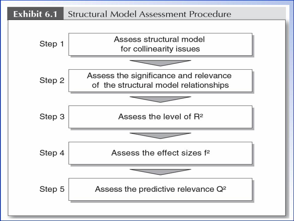
Once the construct measures have been confirmed as reliable and Once the construct measures have been confirmed as reliable and valid, the next step is to assess the structural model results. This valid, the next step is to assess the structural model results. This involves examining the modelinvolves examining the model’’s predictive capabilities and the s predictive capabilities and the relationships between the constructs. Exhibit 6.1 (next slide) shows a relationships between the constructs. Exhibit 6.1 (next slide) shows a systematic approach to the assessment of structural model results.systematic approach to the assessment of structural model results.

Before assessing the structural model, you must examine the Before assessing the structural model, you must examine the structural model for collinearity (Step 1). The reason is that the structural model for collinearity (Step 1). The reason is that the estimation of path coefficients in the structural model is based on OLS estimation of path coefficients in the structural model is based on OLS regressions of each endogenous latent variable on its corresponding regressions of each endogenous latent variable on its corresponding predecessor constructs. Just as in a regular multiple regression, the predecessor constructs. Just as in a regular multiple regression, the path coefficients may be biased if the estimation involves significant path coefficients may be biased if the estimation involves significant levels of collinearity among the predictor constructs.levels of collinearity among the predictor constructs.

After checking for collinearity, the key criteria for assessing the After checking for collinearity, the key criteria for assessing the structural model in PLS-SEM are: Step 2 – the significance of the path structural model in PLS-SEM are: Step 2 – the significance of the path coefficients, Step 3 – the level of the R² values, Step 4 – the f² effect coefficients, Step 3 – the level of the R² values, Step 4 – the f² effect size, and Step 5 – the predictive relevance (Q² & the q² effect size).size, and Step 5 – the predictive relevance (Q² & the q² effect size).

4

Step 1: Collinearity AssessmentStep 1: Collinearity Assessment


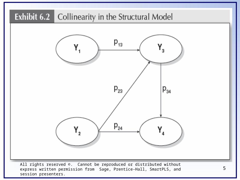
To assess collinearity, we apply the same measures as To assess collinearity, we apply the same measures as in the evaluation of formative measurement model indicators in the evaluation of formative measurement model indicators (i.e., tolerance and VIF values). To do so, we need to examine (i.e., tolerance and VIF values). To do so, we need to examine each set of predictor constructs separately for each subpart of each set of predictor constructs separately for each subpart of the structural model. For instance, in the model shown in the structural model. For instance, in the model shown in Exhibit 6.2 (next slide), Y1 and Y2 jointly explain Y3. Likewise, Exhibit 6.2 (next slide), Y1 and Y2 jointly explain Y3. Likewise, Y2 and Y3 act as predictors of Y4. Therefore, you need to Y2 and Y3 act as predictors of Y4. Therefore, you need to check whether there are significant levels of collinearity check whether there are significant levels of collinearity between each set of predictor variables (constructs). In other between each set of predictor variables (constructs). In other words, you need to check the collinearity between Y1 and Y2 as words, you need to check the collinearity between Y1 and Y2 as well as between Y2 and Y3.well as between Y2 and Y3.

Similar to the assessment of formative measurement Similar to the assessment of formative measurement model indicators, we consider tolerance levels below 0.20 (VIF model indicators, we consider tolerance levels below 0.20 (VIF above 5.00) in the predictor constructs as indicative of above 5.00) in the predictor constructs as indicative of collinearity that is too high. If collinearity is exceeds these collinearity that is too high. If collinearity is exceeds these thresholds, you should consider eliminating constructs, thresholds, you should consider eliminating constructs, merging predictors into a single construct, or creating higher-merging predictors into a single construct, or creating higher-order constructs to deal with collinearity problems. order constructs to deal with collinearity problems.

5All rights reserved ©. Cannot be reproduced or distributed without express written permission from Sage, Prentice-Hall, SmartPLS, and session presenters.


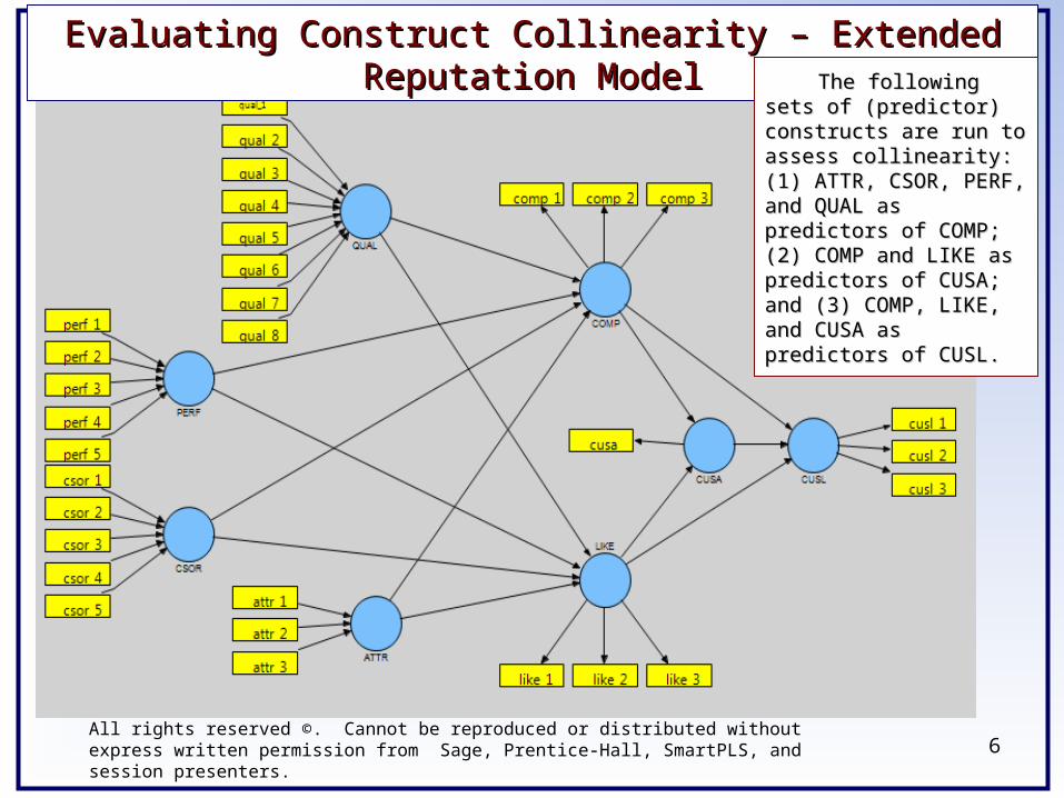
Evaluating Construct Collinearity – Extended Reputation ModelEvaluating Construct Collinearity – Extended Reputation Model

The following sets of The following sets of (predictor) constructs are (predictor) constructs are run to assess collinearity: run to assess collinearity: (1) ATTR, CSOR, PERF, (1) ATTR, CSOR, PERF, and QUAL as predictors of and QUAL as predictors of COMP; (2) COMP and LIKE COMP; (2) COMP and LIKE as predictors of CUSA; and as predictors of CUSA; and (3) COMP, LIKE, and CUSA (3) COMP, LIKE, and CUSA as predictors of CUSL.as predictors of CUSL.

7

..


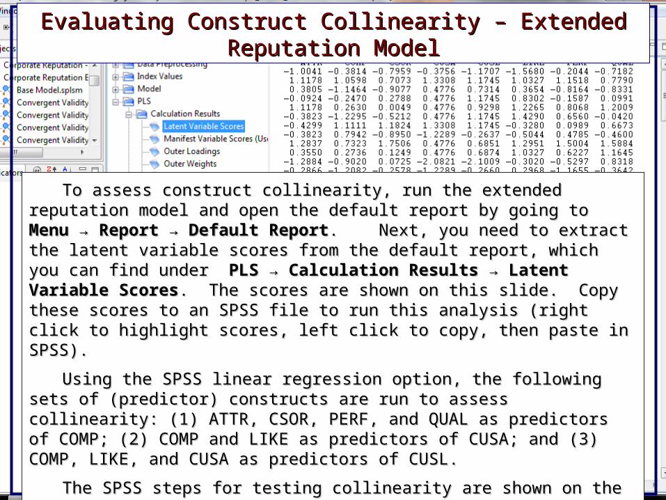
To assess construct collinearity, run the extended reputation model and open To assess construct collinearity, run the extended reputation model and open the default report by going to the default report by going to Menu → Report → Default ReportMenu → Report → Default Report. Next, you . Next, you need to extract the latent variable scores from the default report, which you can need to extract the latent variable scores from the default report, which you can find under find under PLS → Calculation Results → Latent Variable ScoresPLS → Calculation Results → Latent Variable Scores. The scores . The scores are shown on this slide. Copy these scores to an SPSS file to run this analysis are shown on this slide. Copy these scores to an SPSS file to run this analysis (right click to highlight scores, left click to copy, then paste in SPSS).(right click to highlight scores, left click to copy, then paste in SPSS).

Using the SPSS linear regression option, the following sets of (predictor) Using the SPSS linear regression option, the following sets of (predictor) constructs are run to assess collinearity: (1) ATTR, CSOR, PERF, and QUAL as constructs are run to assess collinearity: (1) ATTR, CSOR, PERF, and QUAL as predictors of COMP; (2) COMP and LIKE as predictors of CUSA; and (3) COMP, predictors of COMP; (2) COMP and LIKE as predictors of CUSA; and (3) COMP, LIKE, and CUSA as predictors of CUSL.LIKE, and CUSA as predictors of CUSL.

The SPSS steps for testing collinearity are shown on the next slide for the first The SPSS steps for testing collinearity are shown on the next slide for the first regression run. regression run.

Evaluating Construct Collinearity – Extended Reputation ModelEvaluating Construct Collinearity – Extended Reputation Model

8

..


Using SPSS to Assess CollinearityUsing SPSS to Assess Collinearity

These are the These are the four exogenous four exogenous

constructs that are constructs that are being tested for being tested for multicollinearity.multicollinearity.

9

Below are the SPSS collinearity results from using Below are the SPSS collinearity results from using ATTR, CSOR, PERF, and QUAL as predictors of COMP. ATTR, CSOR, PERF, and QUAL as predictors of COMP.


Evaluating Collinearity Among Exogenous ConstructsEvaluating Collinearity Among Exogenous Constructs

All VIF values All VIF values are clearly below are clearly below

the threshold of 5. the threshold of 5.


Below are the collinearity results from using COMP and LIKE as Below are the collinearity results from using COMP and LIKE as predictors of CUSA (top table), and COMP, LIKE and CUSA as predictors of predictors of CUSA (top table), and COMP, LIKE and CUSA as predictors of CUSL (bottom table). All VIF values are well below the threshold of 5. CUSL (bottom table). All VIF values are well below the threshold of 5.

Evaluating Collinearity Among Exogenous ConstructsEvaluating Collinearity Among Exogenous Constructs

11

Step 2: Assess Significance and Relevance Step 2: Assess Significance and Relevance of the Structural Model Relationshipsof the Structural Model Relationships


After applying the PLS-SEM algorithm, estimates are After applying the PLS-SEM algorithm, estimates are obtained for the structural model relationships (the path obtained for the structural model relationships (the path coefficients), which represent the hypothesized relationships coefficients), which represent the hypothesized relationships between the constructs.between the constructs.

The path coefficients for the structural model are shown The path coefficients for the structural model are shown in the next several slides. These results were obtained from in the next several slides. These results were obtained from the SmartPLS Default Report with the following sequence: the SmartPLS Default Report with the following sequence:

PLS Algorithm PLS Algorithm → → Calculation Results Calculation Results → → Path CoefficientsPath Coefficients

Before examining the sizes of the path coefficients we Before examining the sizes of the path coefficients we will first examine their significance. To do so, we must first will first examine their significance. To do so, we must first run the Bootstrapping option. run the Bootstrapping option.


Reputation Model ResultsReputation Model Results– – Path Coefficients – Path Coefficients –


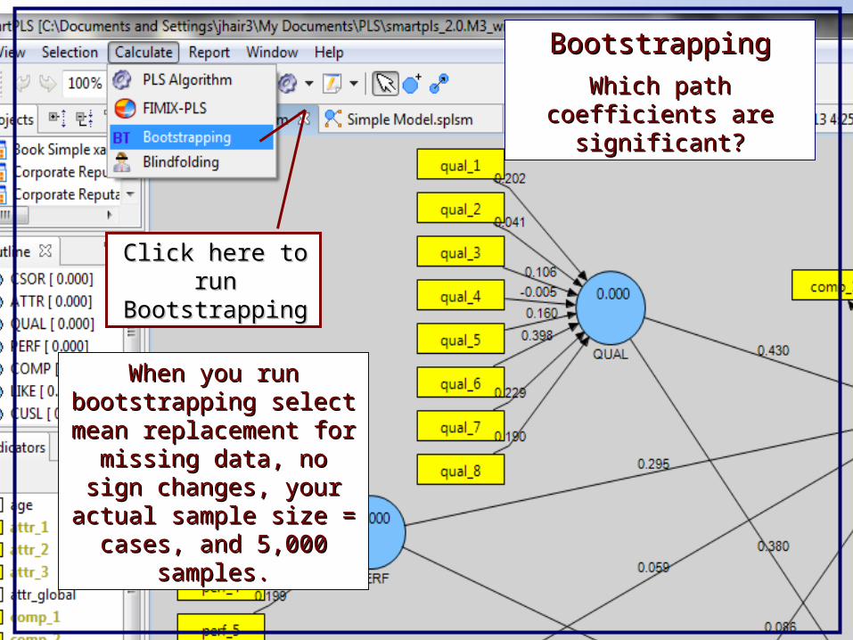
Click here to run Click here to run BootstrappingBootstrapping

BootstrappingBootstrapping

Which path coefficients Which path coefficients are significant?are significant?

When you run When you run bootstrapping select bootstrapping select

mean replacement for mean replacement for missing data, no sign missing data, no sign changes, your actual changes, your actual sample size = cases, sample size = cases, and 5,000 samples.and 5,000 samples.

..


Bootstrapping Default Report – Significance of Path CoefficientsBootstrapping Default Report – Significance of Path Coefficients

The above results show the significance of the path coefficients. Recall that The above results show the significance of the path coefficients. Recall that a T Statistic > 1.96 is significant with a two-tailed test, and >.98 is significant for a a T Statistic > 1.96 is significant with a two-tailed test, and >.98 is significant for a one-tailed test. Note: path coefficients are shown in Original Sample column.one-tailed test. Note: path coefficients are shown in Original Sample column.

The results indicate that all paths are statistically significant using a one-tailed The results indicate that all paths are statistically significant using a one-tailed test except COMP – CUSL. But eight of the thirteen structural paths are test except COMP – CUSL. But eight of the thirteen structural paths are significant based on a two-tailed test.significant based on a two-tailed test.

14

T Statistics are found T Statistics are found beside the tab below.beside the tab below.


Click here to obtain Click here to obtain Default Report Default Report

Obtaining the Default Report Obtaining the Default Report to Evaluate Path Coefficientsto Evaluate Path Coefficients


SmartPLS Default Report – Path CoefficientsSmartPLS Default Report – Path Coefficients

After examining the significance of relationships, it is important to assess the After examining the significance of relationships, it is important to assess the relevance of significant relationships. Path coefficients in the structural model relevance of significant relationships. Path coefficients in the structural model may be significant, but their size may be so small that they do not warrant may be significant, but their size may be so small that they do not warrant managerial attention. managerial attention.

Structural model path coefficients can be interpreted relative to one another. Structural model path coefficients can be interpreted relative to one another. If one path coefficient is larger than another, its effect on the endogenous latent If one path coefficient is larger than another, its effect on the endogenous latent variable is greater. More specifically, the individual path coefficients of the path variable is greater. More specifically, the individual path coefficients of the path model can be interpreted just as the standardized beta coefficients in an OLS model can be interpreted just as the standardized beta coefficients in an OLS regression. These coefficients represent the estimated change in the regression. These coefficients represent the estimated change in the endogenous construct for a unit change in a predictor construct. endogenous construct for a unit change in a predictor construct.


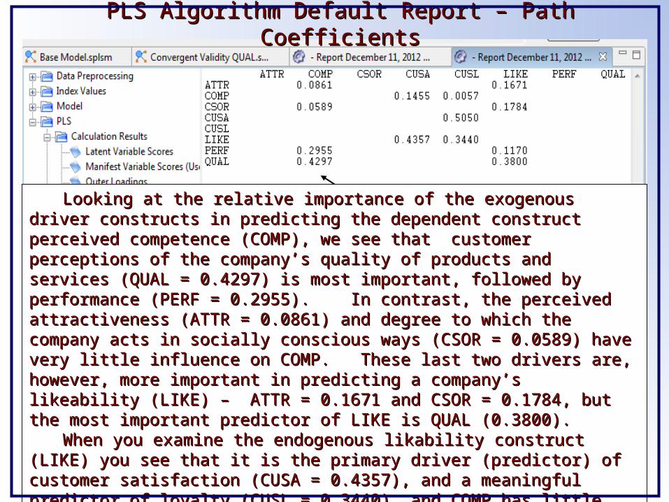
Looking at the relative importance of the exogenous driver constructs in Looking at the relative importance of the exogenous driver constructs in predicting the dependent construct perceived competence (COMP), we see that predicting the dependent construct perceived competence (COMP), we see that customer perceptions of the companycustomer perceptions of the company’’s quality of products and services (QUAL = s quality of products and services (QUAL = 0.4297) is most important, followed by performance (PERF = 0.2955). In 0.4297) is most important, followed by performance (PERF = 0.2955). In contrast, the perceived attractiveness (ATTR = 0.0861) and degree to which the contrast, the perceived attractiveness (ATTR = 0.0861) and degree to which the company acts in socially conscious ways (CSOR = 0.0589) have very little company acts in socially conscious ways (CSOR = 0.0589) have very little influence on COMP. These last two drivers are, however, more important in influence on COMP. These last two drivers are, however, more important in predicting a companypredicting a company’’s likeability (LIKE) – ATTR = 0.1671 and CSOR = 0.1784, s likeability (LIKE) – ATTR = 0.1671 and CSOR = 0.1784, but the most important predictor of LIKE is QUAL (0.3800).but the most important predictor of LIKE is QUAL (0.3800).

When you examine the endogenous likability construct (LIKE) you see that it When you examine the endogenous likability construct (LIKE) you see that it is the primary driver (predictor) of customer satisfaction (CUSA = 0.4357), and a is the primary driver (predictor) of customer satisfaction (CUSA = 0.4357), and a meaningful predictor of loyalty (CUSL = 0.3440), and COMP has little impact on meaningful predictor of loyalty (CUSL = 0.3440), and COMP has little impact on CUSL (0.0057).CUSL (0.0057).

PLS Algorithm Default Report – Path CoefficientsPLS Algorithm Default Report – Path Coefficients

18

Understanding Direct and Indirect EffectsUnderstanding Direct and Indirect Effects


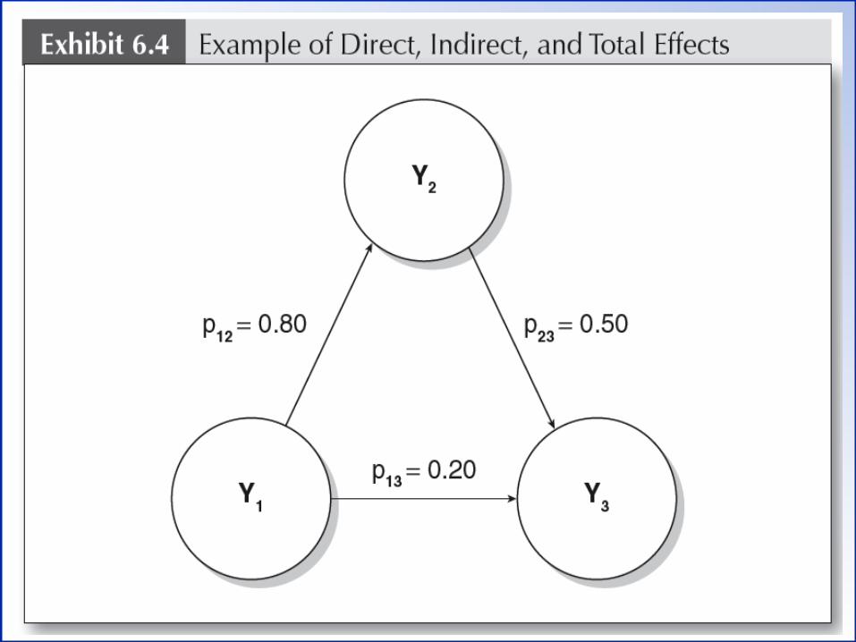
Researchers are often interested in evaluating not only Researchers are often interested in evaluating not only one constructone construct’’s s direct effect direct effect on another but also its on another but also its indirect indirect effects effects via one or more mediating constructs. The sum of via one or more mediating constructs. The sum of direct and indirect effects is referred to as the direct and indirect effects is referred to as the total effect. total effect.

In Exhibit 6.4 on the next slide, constructs YIn Exhibit 6.4 on the next slide, constructs Y11 and Y and Y33 are are linked by a direct effect (plinked by a direct effect (p1313 = 0.20). In addition, there is an = 0.20). In addition, there is an indirect effect between the two constructs via the mediating indirect effect between the two constructs via the mediating construct Yconstruct Y22. This indirect effect can be calculated as the . This indirect effect can be calculated as the product of the two effects pproduct of the two effects p1212 and p and p2323 (p (p1212 x p x p2323 = 0.80 x 0.50 = = 0.80 x 0.50 = 0.40). The total effect is 0.60, which is calculated as p0.40). The total effect is 0.60, which is calculated as p1313 + (p + (p1212 x px p2323) = 0.20 + (0.80 x 0.50) = 0.20 + 0.40 = 0.60.) = 0.20 + (0.80 x 0.50) = 0.20 + 0.40 = 0.60.

Although the direct effect of YAlthough the direct effect of Y11 to Y to Y33 is not very strong is not very strong (i.e., 0.20), the total effect (both direct and indirect combined) (i.e., 0.20), the total effect (both direct and indirect combined) is quite pronounced (i.e., 0.60), indicating the relevance of Yis quite pronounced (i.e., 0.60), indicating the relevance of Y11 in in explaining Yexplaining Y33. This type of result suggests that the direct . This type of result suggests that the direct relationship from Yrelationship from Y11 to Y to Y33 is mediated by Y is mediated by Y22. .

20

PLS Algorithm Default Report – Total Effects = SizesPLS Algorithm Default Report – Total Effects = Sizes


The four driver constructs for loyalty (CUSL) are the exogenous The four driver constructs for loyalty (CUSL) are the exogenous constructs on the left side of the SEM model (these constructs are constructs on the left side of the SEM model (these constructs are actionable because they are formative and thus of primary concern actionable because they are formative and thus of primary concern for the total effects analysis). The findings shown above indicate that for the total effects analysis). The findings shown above indicate that quality (QUAL = 0.2483) has the strongest total effect on loyalty, quality (QUAL = 0.2483) has the strongest total effect on loyalty, followed by corporate social responsibility (CSOR = 0.1053), followed by corporate social responsibility (CSOR = 0.1053), attractiveness (ATTR = 0.1010), and performance (PERF = 0.0894). attractiveness (ATTR = 0.1010), and performance (PERF = 0.0894).

Note that there are three mediating constructs (COMP, CUSA & Note that there are three mediating constructs (COMP, CUSA & LIKE) between the exogenous driver constructs and the endogenous LIKE) between the exogenous driver constructs and the endogenous construct CUSL whose role must be considered, but they are construct CUSL whose role must be considered, but they are relatively less actionable because they are reflective – not formative.relatively less actionable because they are reflective – not formative.


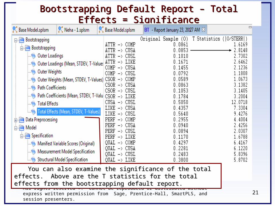
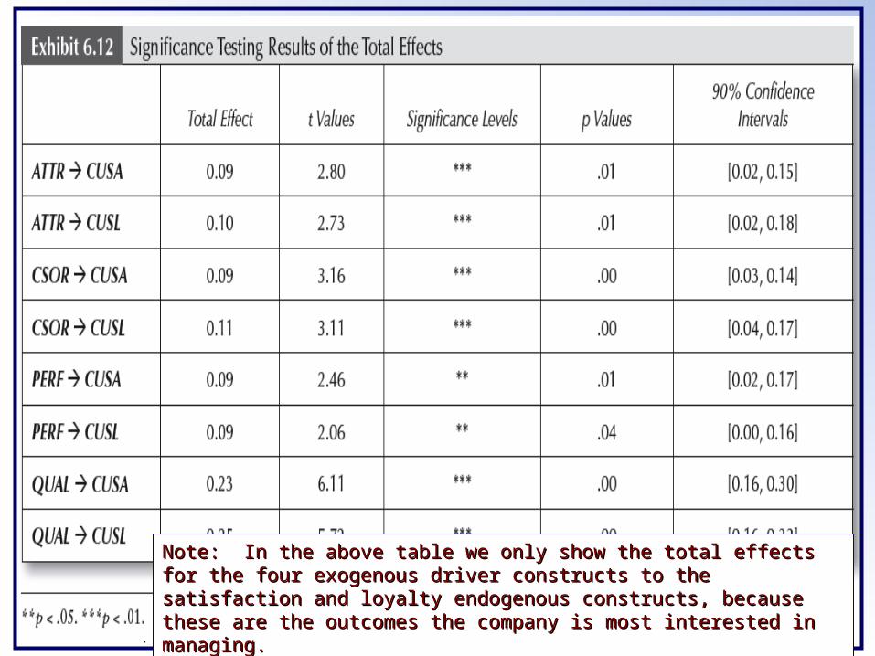
Bootstrapping Default Report – Total Effects = SignificanceBootstrapping Default Report – Total Effects = Significance

You can also examine the significance of the total effects. Above are You can also examine the significance of the total effects. Above are the T statistics for the total effects from the bootstrapping default report.the T statistics for the total effects from the bootstrapping default report.

22

..


Note: In the above table we only show the total effects for the four exogenous Note: In the above table we only show the total effects for the four exogenous driver constructs to the satisfaction and loyalty endogenous constructs, driver constructs to the satisfaction and loyalty endogenous constructs, because these are the outcomes the company is most interested in managing.because these are the outcomes the company is most interested in managing.

23

To get outer weights: To get outer weights: PLS PLS → → Calculation Results Calculation Results → → Outer WeightsOuter Weights

By examining the outer weights of the construct indicators, we can identify which By examining the outer weights of the construct indicators, we can identify which specific element of quality (QUAL) needs to be addressed. Note that specific element of quality (QUAL) needs to be addressed. Note that qual_6 qual_6 has the has the highest outer weight (0.3980). This survey question was highest outer weight (0.3980). This survey question was ““[the company] seems to be [the company] seems to be a reliable partner for customersa reliable partner for customers”” so perceptions of reliability should be enhanced and so perceptions of reliability should be enhanced and communicated to customers.communicated to customers.

Identifying actionable Identifying actionable strategies based on strategies based on sizes of exogenous sizes of exogenous construct weights.construct weights.

Download - 1 Using the SmartPLS Software “Structural Model Assessment” All rights reserved ©. Cannot be reproduced or distributed without express written permission

Top Related