06 - Boundary Models
• Overview• Edge Tracking• Active Contours• Conclusion
Overview
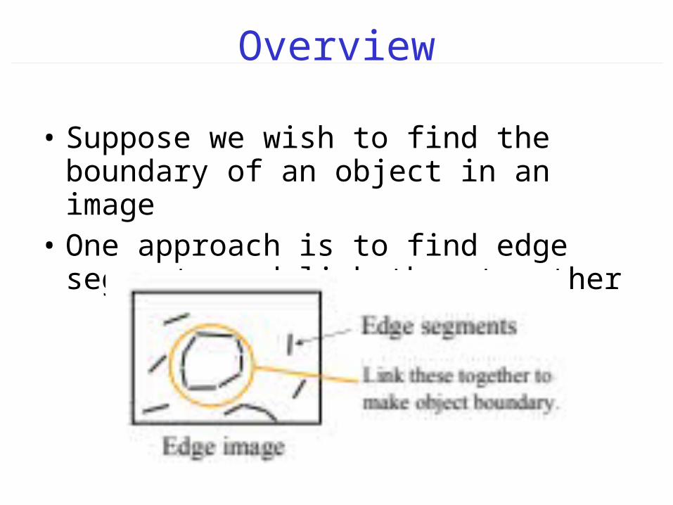
• Suppose we wish to find the boundary of an object in an image
• One approach is to find edge segments and link them together

Overview
• The process of linking edge segments to obtain boundary models is deceptively difficult– How do we select edge segments for the object? – How do connect these edge segments? – What do we do with missing or conflicting data?– What domain knowledge can be used?– How much user input is necessary?– How do measure the quality of our solution?

Overview
• In this section we will consider the design and implementation of two techniques
• Edge tracking – performs a greedy search to find a path around the object boundary
• Active contours – solves for object boundary by minimizing an energy functional that describes constraints on the object boundary
Edge Tracking
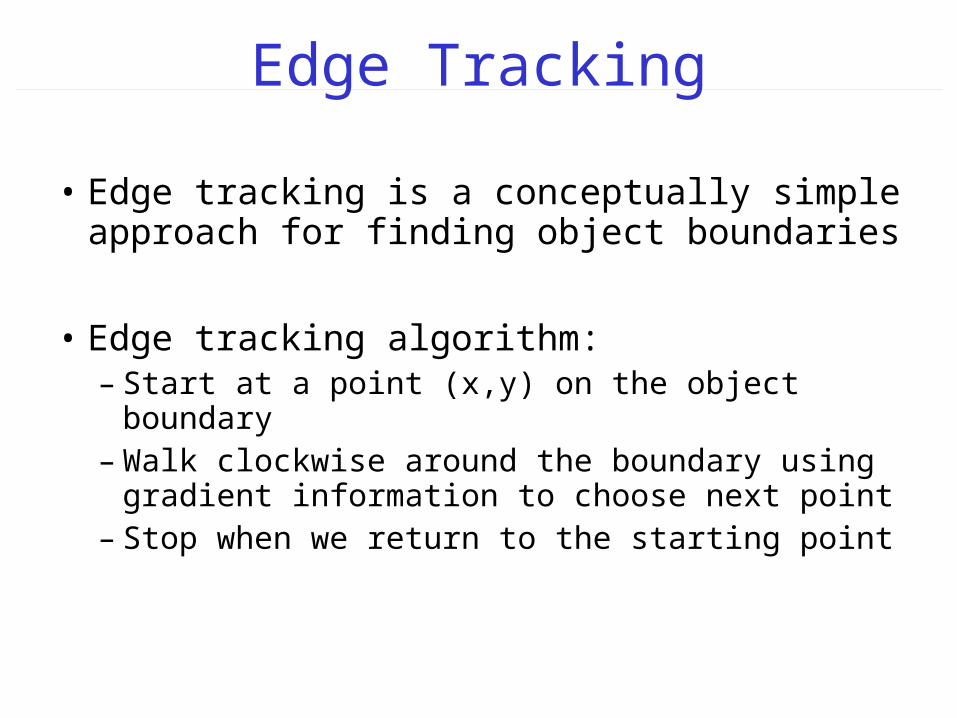
• Edge tracking is a conceptually simple approach for finding object boundaries
• Edge tracking algorithm:– Start at a point (x,y) on the object boundary– Walk clockwise around the boundary using
gradient information to choose next point– Stop when we return to the starting point
Edge Tracking
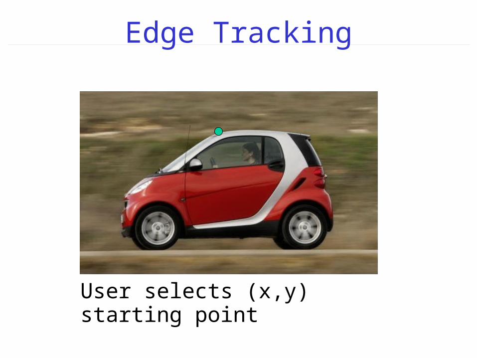
User selects (x,y) starting point

Edge Tracking
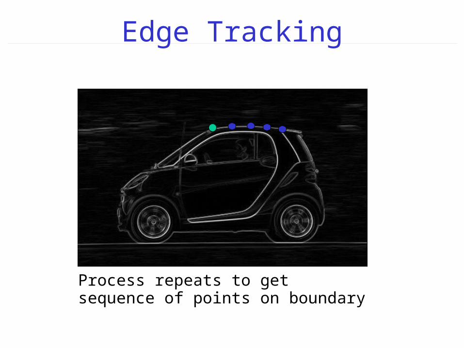
Gradient information used to find next (x,y) point on boundary
Edge Tracking
Process repeats to get sequence of points on boundary
Edge Tracking
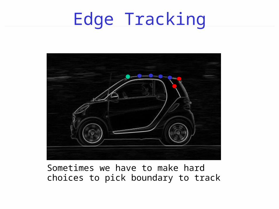
Sometimes we have to make hard choices to pick boundary to track
Edge Tracking
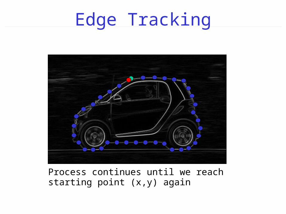
Process continues until we reach starting point (x,y) again
Edge Tracking
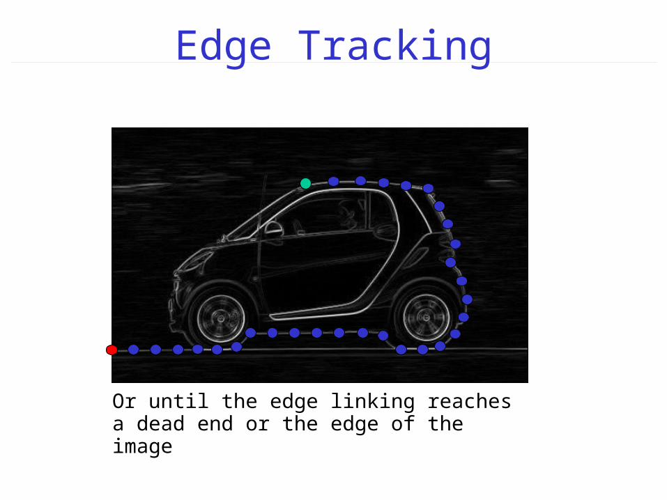
Or until the edge linking reaches a dead end or the edge of the image
Edge Tracking
• If we are at pixel (x,y) on the boundary how do we select next point (x’,y’) on boundary?
• There are a number of factors to consider:– Find point with highest gradient magnitude– Find point with most similar gradient magnitude– Find point with most similar gradient direction– Find point that gives smoothest boundary
Edge Tracking
• To find point with highest gradient magnitude– Calculate gradient magnitude of image– Search NxN neighborhood around point (x,y)– Ignore points that are already on object boundary– Find point (x’,y’) that has the highest gradient
magnitude value G
• Very simple to implement, but might get stuck in local gradient maxima
Edge Tracking
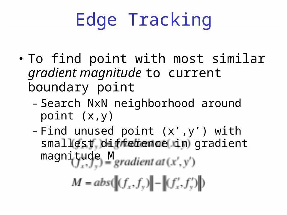
• To find point with most similar gradient magnitude to current boundary point– Search NxN neighborhood around point (x,y)– Find unused point (x’,y’) with smallest difference
in gradient magnitude M
Edge Tracking
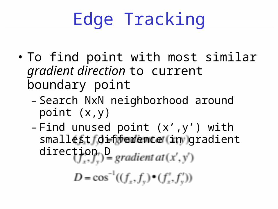
• To find point with most similar gradient direction to current boundary point– Search NxN neighborhood around point (x,y)– Find unused point (x’,y’) with smallest difference
in gradient direction D
Edge Tracking
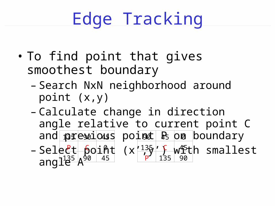
• To find point that gives smoothest boundary– Search NxN neighborhood around point (x,y)– Calculate change in direction angle relative to
current point C and previous point P on boundary– Select point (x’,y’) with smallest angle A
135 90 45
P C 0135 90 45
90 45 0
135 C 45P 135 90
Edge Tracking
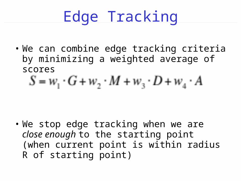
• We can combine edge tracking criteria by minimizing a weighted average of scores
• We stop edge tracking when we are close enough to the starting point (when current point is within radius R of starting point)

Edge Tracking
• Edge tracking works well when the edge strengths are strong in an image and the user provides a good starting point on the edge
• Edge tracking works poorly if there are weak or missing edges since there are no global constraints on the shape of object boundary
Active Contours
• Edge tracking approach may produce very rough object boundaries– No boundary smoothness constraints
• Active contours solves this problem– Define object boundary as a parametric curve– Define smoothness constraints on the curve– Define data matching constraints on the curve– Deform curve to find optimal object boundary
Active Contours
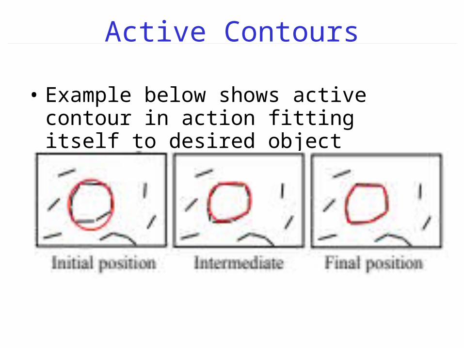
• Example below shows active contour in action fitting itself to desired object boundary
Active Contours
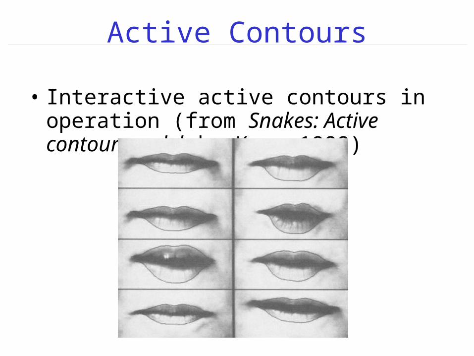
• Interactive active contours in operation (from Snakes: Active contour models by Kass 1988)
Active Contours
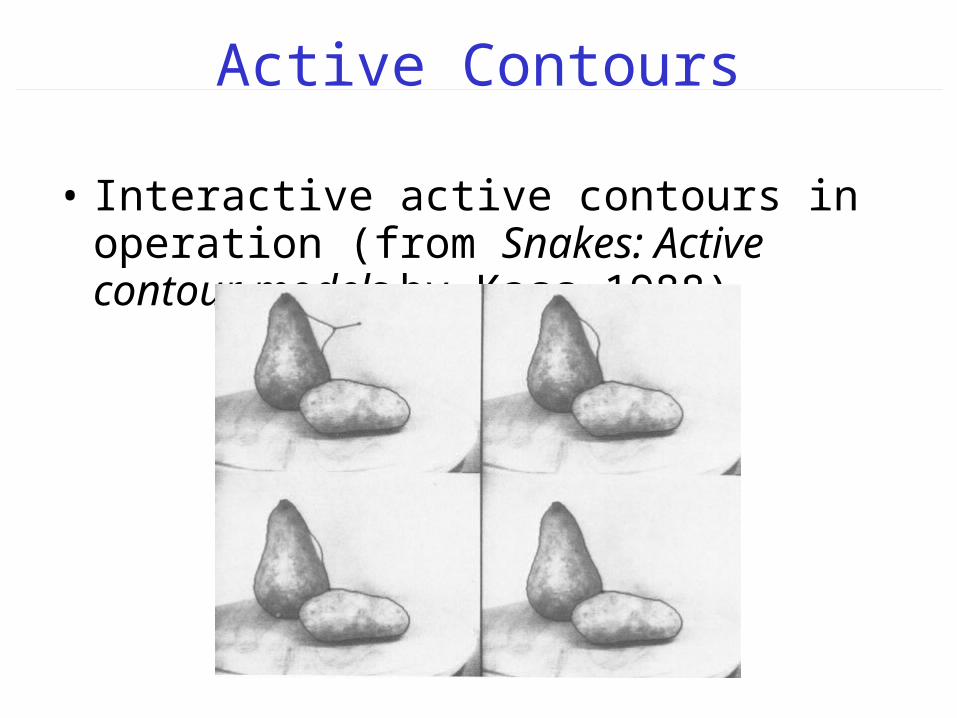
• Interactive active contours in operation (from Snakes: Active contour models by Kass 1988)
Active Contours
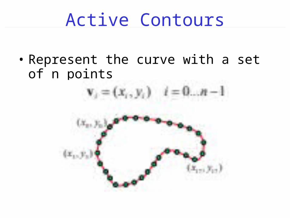
• Represent the curve with a set of n points
Active Contours
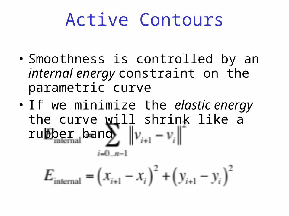
• Smoothness is controlled by an internal energy constraint on the parametric curve
• If we minimize the elastic energy the curve will shrink like a rubber band
Active Contours
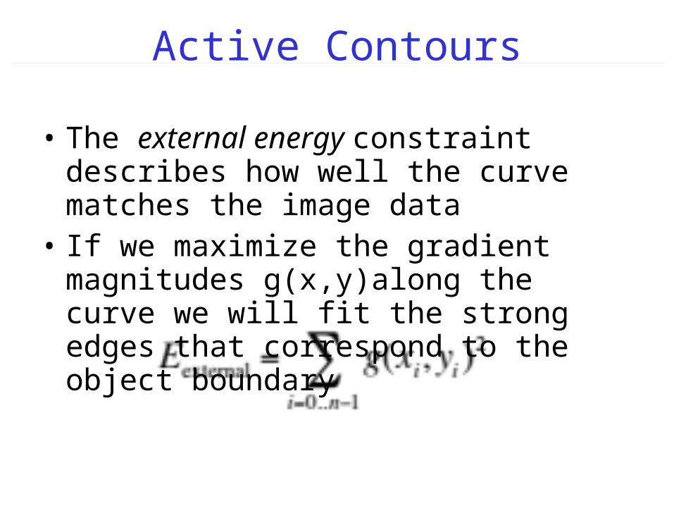
• The external energy constraint describes how well the curve matches the image data
• If we maximize the gradient magnitudes g(x,y)along the curve we will fit the strong edges that correspond to the object boundary
Active Contours
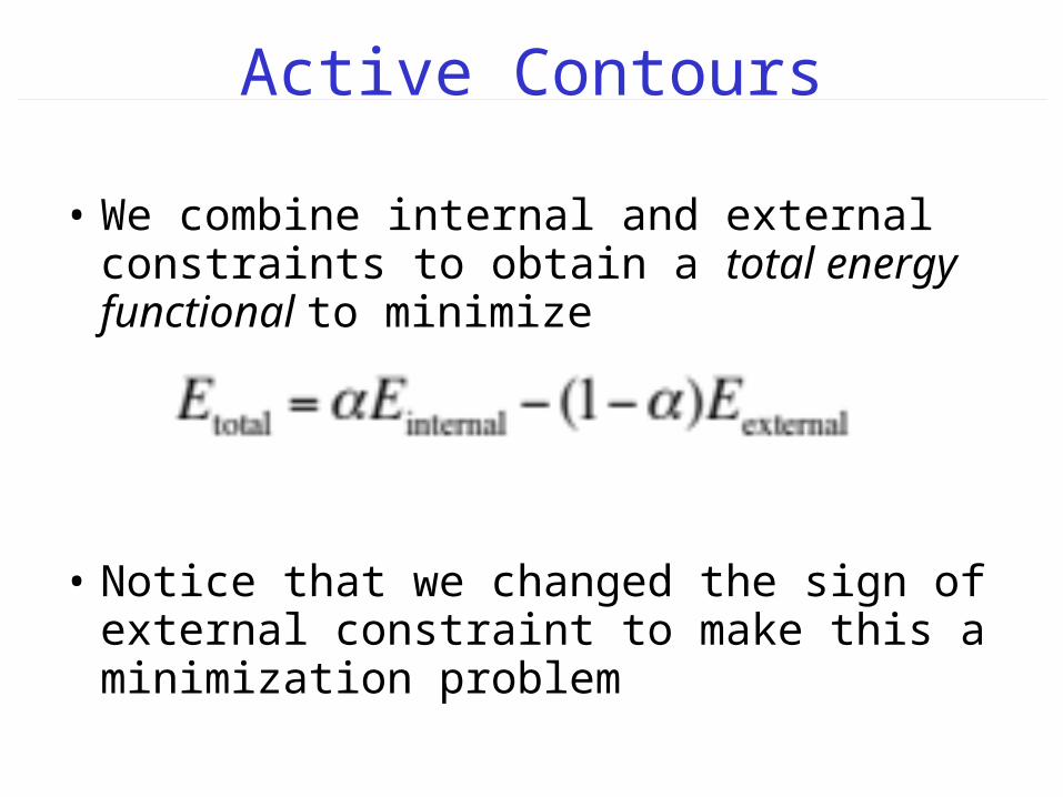
• We combine internal and external constraints to obtain a total energy functional to minimize
• Notice that we changed the sign of external constraint to make this a minimization problem
Active Contours
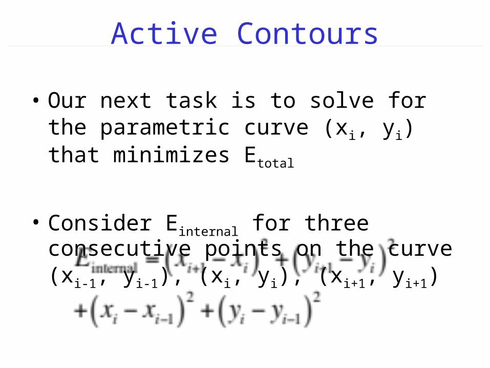
• Our next task is to solve for the parametric curve (xi, yi) that minimizes Etotal
• Consider Einternal for three consecutive points on the curve (xi-1, yi-1), (xi, yi), (xi+1, yi+1)
Active Contours
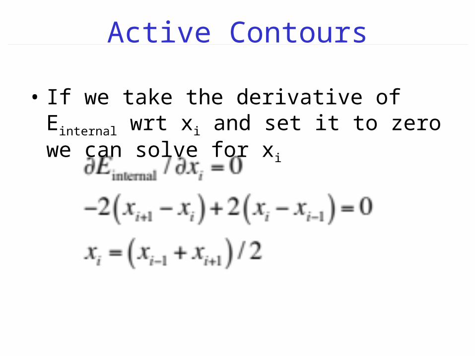
• If we take the derivative of Einternal wrt xi and set it to zero we can solve for xi
Active Contours
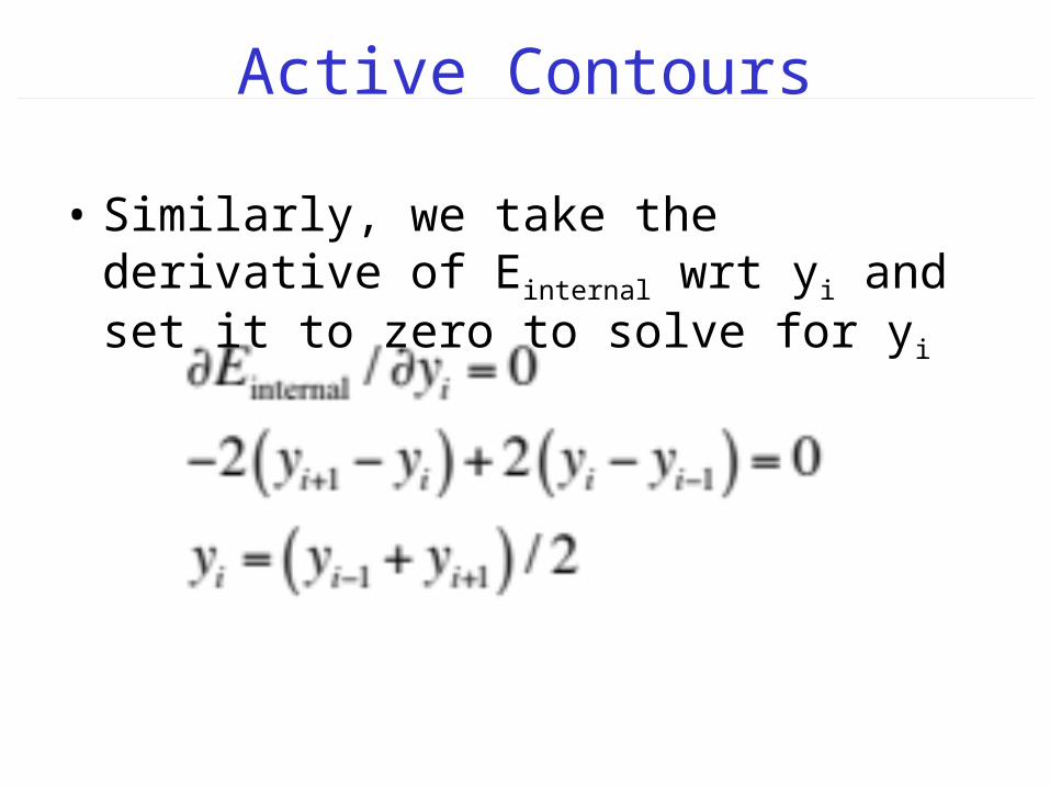
• Similarly, we take the derivative of Einternal wrt yi and set it to zero to solve for yi

Active Contours
• Hence we can deform the active contour to minimize the internal energy by iteratively averaging adjacent boundary coordinates
(xi-1,yi-1)
(xi,yi)
(xi+1,yi+1)
Active Contours
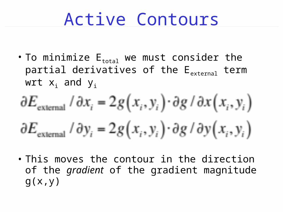
• To minimize Etotal we must consider the partial derivatives of the Eexternal term wrt xi and yi
• This moves the contour in the direction of the gradient of the gradient magnitude g(x,y)
Active Contours
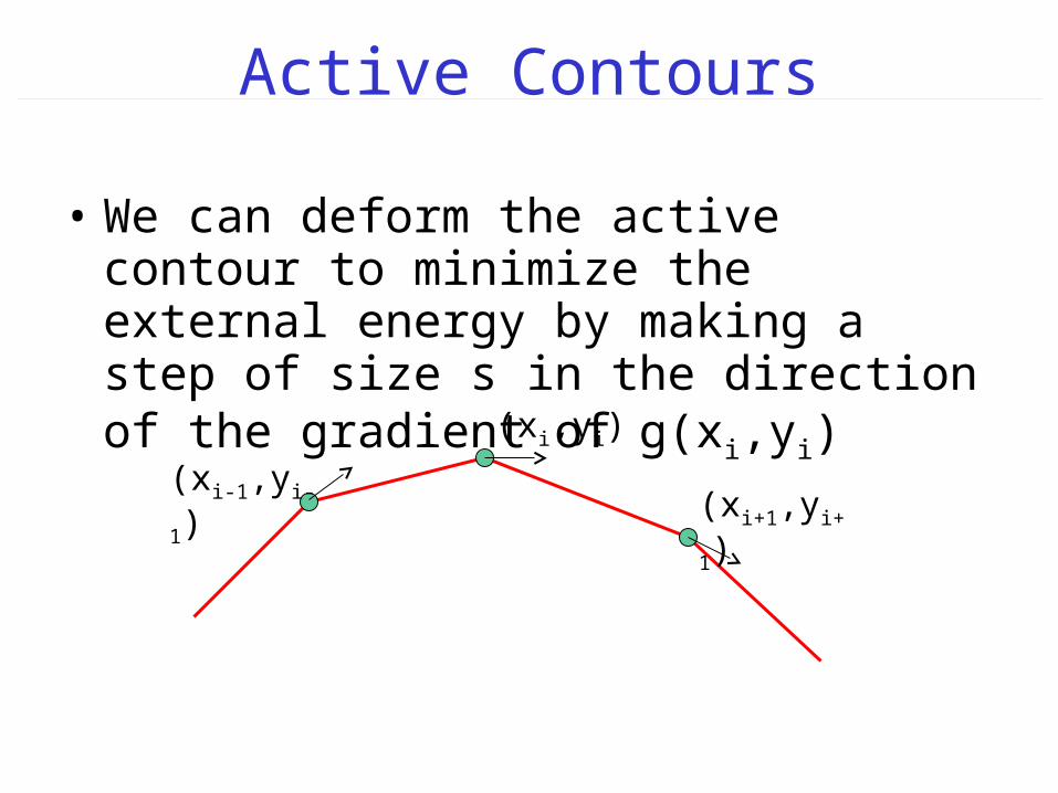
• We can deform the active contour to minimize the external energy by making a step of size s in the direction of the gradient of g(xi,yi)
(xi-1,yi-1)
(xi,yi)
(xi+1,yi+1)
Active Contours
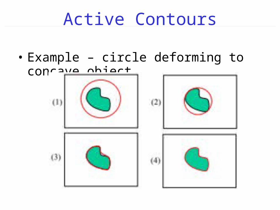
• Example – circle deforming to concave object
Active Contours
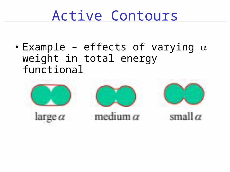
• Example – effects of varying weight in total energy functional

Active Contours
• Example – fitting one active contour around two adjacent objects
Active Contours
• Additional constraints can be added to active contours to introduce stiffness (minimize second derivatives) and other external forces (user pulling curve at selected points)
• Calculus of variations is typically used to solve the Euler-Legrange equations associated with these active contour energy functionals
Conclusions
• This section described how boundary tracking and active contours can be used to obtain the boundary of objects of interest in an image
• Both methods require user interaction to select a starting point/curve – Boundary tracking fast and easy to implement– Active contours will result in smoother boundary


