double teaching optimization for short term hydro thermal...

International Journal on Electrical Engineering and Informatics - Volume 9, Number 2, June 2017

Double Teaching Optimization for Short Term Hydro

Thermal Scheduling Problem

Ajit Kumar Barisal1, Ramesh Chandra Pusty1, Kumadini Suna1

and Tapas Kumar Panigrahi2

1Department of Electrical Engineering, Veer Surendra Sai University of Technology,

Burla, Odisha, India. 2Department of Electrical & Electronics Engineering, IIIT, Bhubaneswar, Odisha, India.

[email protected]

Abstracts: This paper presents an efficient and reliable new teaching based optimization

algorithm for solving scheduling of hydro-thermal systems with cascaded reservoirs. Unlike

the Teaching Learning Based Optimization, the Double Teaching Optimization (DTO)

algorithm has two teaching phases i.e. the first teaching phase is identical with conventional

TLBO algorithm preserving the inherent basics of it. The second teaching phase is the

modified part considering students once again interact with the same teacher, who is the better

than average students called double teaching phase. The feasibility of the proposed method is

demonstrated in five different cases of two standard test systems consisting of four cascaded

hydro and thermal units. The findings of the proposed method are better than the results of

other established methods reported in literature in terms of quality of solution and convergence

characteristics.

Keywords: Hydrothermal scheduling, cascaded reservoir, differential evolution, double

teaching optimization, teaching learning based optimization, prohibited operating zone, valve

point loading effect.

1. Introduction

Over the last few decades, we experience energy crisis and ill effects of pollution to save

nation, so it is very important to utilize energy in an efficient manner. In order to utilize energy

efficiently, cost must be as less as possible and this possesses a requirement to develop

scheduling methods that accommodate generation diversity and line flow limitations and

concurrently can produce accurate scheduling results. Again the power generation is much

lesser as compared to power demand in our country, so the main aim of power system

operation is to generate and transmit power to meet the system load demand and losses at

minimum fuel cost and minimum environmental pollution. Hence, a mixed of hydrothermal

scheduling is necessary. The short range hydrothermal problem has usually as an optimization

interval of one day or week. This period is normally subdivided into subintervals for

scheduling purposes. Here the load demand, water inflow and discharge of water are known. A

set of starting condition that means the reservoirs storage level is being given. The optimal

power schedule can be prepared that can minimize the desired objective while meeting the

system constraints successfully. In order to solve the scheduling problem of short term hydro-

thermal systems, the head of water level is assumed to be constant. The objective of short term

hydrothermal scheduling of power system is to determine the optimal hydro and thermal

generations in order to meet the load demands over a scheduling horizon of time while

Received: January 16th, 2016. Accepted: June 22nd, 2017

DOI: 10.15676/ijeei.2017.9.2.9

322

mailto:[email protected]

satisfying the various operational constraints imposed on the hydraulic and thermal power

system network. The optimal scheduling of hydrothermal power system is usually more

complex than that for all thermal system. It is basically a non-linear problem involving

nonlinear objective function and a mixture of linear and non-linear constraints on thermal

plants as well as hydroelectric plants [1-2].

Dynamic programming (DP) [3,4] method have been employed in solving most economical

hydro thermal generation schedule under the practical constraints. However, this method is

suffering from the curse of dimensionality and local optimality. Many stochastic search

algorithms like artificial neural network [5],simulated annealing technique [6], a coordinated

approach [7], genetic algorithm [8], evolutionary programming (EP) [9], two phase neural

network approach [10], fast evolutionary programming [11], fuzzy interactive EP [12],

simulated annealing based goal attainment method[13], an efficient real coded GA [14],

modified differential evolution (MDE) [15], improved particle swarm optimization (IPSO)

[16,18], biogeography based optimization [17], clonal selection algorithm [19], an adaptive

artificial bee colony optimization [21], a mixed binary evolutionary particle swarm optimizer

[22], teaching learning based optimization (TLBO) [23] and improved DE [24] have applied

successfully to solve hydrothermal problems.

The neural network [5,10] based approaches may suffer from excessive numerical

iterations. Simulated annealing (SA) [6,12] requires appropriate annealing schedule otherwise

achieved solution will be of locally optimal. Genetic algorithm [8,14] is commonly used

evolutionary technique and is based on selection, crossover and mutation operation. However it

suffered from premature convergence which may lead to a local optimal solution. In

differential evolution [15,24] algorithm, it is difficult to properly choose the control parameter.

The literature survey of improved particle swarm optimization (IPSO) [16,18,22] reveals that

this technique is able to generate high quality solutions with less computational time, but

sometimes trapped by local optima. Krill herd algorithm (KHA) [25] technique and symbiotic

organisms search (SOS) algorithm [26] have been successfully employed to solve the short-

term hydrothermal scheduling (HTS) problem by Roy et.al. and Das et.al, respectively.

Teaching learning based optimization is a derivative free optimization and no control

parameters for tuning applied successfully in various large scale problems [20, 23]. This paper

proposes modified teaching learning based optimization called as double teaching optimization

(DTO) for short term optimal scheduling of generation in a hydro thermal system which

involves the allocation of generations among the multi reservoir cascaded hydro plants having

prohibited operating zones and thermal units with valve point loading so as to minimize the

total fuel cost of thermal plants while satisfying the various constraints imposed on hydraulic

and thermal network. To verify the superiority of the proposed approach, two hydrothermal

systems have been considered in this study. The first test system consists of a multi-chain

cascade of four hydro units and one thermal unit and second test system with same cascaded

four hydro units and three thermal units. The results obtained by proposed DTO method are

compared with other population based intelligent algorithms and found to be better not only in

operating cost but also in convergence property in achieving the optimal solution.

2. Problem Formulation of Short Term Hydro Thermal Scheduling

The objective of the short term scheduling of a multiple hydro-thermal system over a

schedule horizon to meet the load demand is to schedule the hydro and thermal plants

Ajit Kumar Barisal, et al.

323

generation in such a way that minimizes the generation cost without violating any constraints

imposed on hydro and thermal plants.

A. Objective function

As the fuel cost of hydropower plants are insignificant in comparison with that of thermal

power plants, so the main objective of the HTS is to minimize the fuel cost of thermal units

while making use of availability of hydro resource as much as possible. The objective function

of HTS problem for thermal units having quadratic cost function is given by

Minimize ijii

nt

i

NH

j

jii cPTbPTaPTFC

,

1 1

2,

(1)

Where nt is the number of thermal generating units and NH is the number of time intervals.

The fuel cost function of each thermal generating unit considering the valve point effects is

expressed as the sum of quadratic and sinusoidal function. Thus the fuel cost function with

valve point effects can be expressed as

Minimize jiiiiijii

nt

i

NH

j

jii PTPTedcPTbPTaPTFC ,min,

1 1

2, sin

(2)

B. Equality Constraints

(i) power balance constraints

The total active power generation must balance the predicted power demand and the

transmission loss at each time interval over the scheduling horizon and it may be

mathematically expressed as

jij

nt

i

ji

nh

i

ji PLPDPTPH ,

1

,

1

,

(3)

Where the hydro electric generation is a function of water discharge rate and storage

volume, which can be expressed as follows:

ijiijiijijiijiijiiji CQCVCQVCQCVCPH ,6,,5,,4,,,3

2,,2

2,,1, (4)

(ii) Initial and final reservoir storage constraints: Initial and final reservoir volumes are

generally set by the midterm scheduling process. This equality constraint implies that the total

quantity of available water is fully utilized. This equality constraint is mathematically

expressed as follows:

beginii VV 1,

; endii VV 25,

(5)

(iii) Reservoir flow balance: In this constraint, water transportation delay between reservoirs is

considered. The flow balance equation relates the water storage volume during previous

interval with the current storage, net inflow, discharge and spillage. This may mathematically

be expressed as follows:

uR

u

jujuijji sQVV

1

)1( 111 jijiji IsQ for j =1,2,…, NH (6)


324

C. Inequality constraints

(i) Power generation constraints: Active power generation of each hydro and thermal power

plant in each hour is bounded between its upper and lower limits as given below:

ijii PHPHPH max,min , (7)

ijii PTPTPT max,min , Where nhi ,...,...2,1 , and NHj ,...,...2,1 (8)

(ii) Reservoir water storage constraints: The water storage capacity of each hydro power plant

reservoir at each hour must be within its minimum and maximum limits as given below:

ijii VVV max,min , Where nhi ,...,...2,1 , and NHj ,...,...2,1 (9)

(iii) Water discharge constraints: The water discharge limit of each hydro power plant

reservoir at each hour must be within its minimum and maximum limits as given below:

ijii QQQ max,min (10)

3. Double Teaching Optimization (DTO) Algorithm

This algorithm mainly emphasizes the importance of teacher on the students to increase the

mean results of whole class room. Learning phase of TLBO algorithm allows the student–

student interaction through group discussion, mutual interaction etc which does not show much

improvement in cost rather it unnecessary increases the computational time. In DTO algorithm

the learning phase is being neglected and modified. The students once again are allowed to

interact with teacher only as the teacher is considered as best among all students, most

respected and knowledgeable person in the society and they always motivate the students to

attain their goal and this is accomplished by increasing the number of interactions. There are

two teaching phases in the proposed algorithm. So, the teacher–student interaction is better

than the student-student interaction as the teacher is a scholar better than the average students

and ensuring the transformation of quality education in second phase of teaching in a class

room i.e. learner phase is neglected. This Double Teaching Optimization (DTO) is also called

as double teaching phases based method. The DTO algorithm has certain control parameters

i.e. mutation rate, population size and maximum iteration number.

A. First teaching phase:

Here, the students improve their knowledge with the help of teacher and the teacher tries his

best to enhance the average results of class room. The teacher always improves the average

grade of the class to some extent. If the new average grade of the thj subject at

thk iteration is

k

newj , the difference between the existing mean k

j and new mean of the thj subject at the

thk iteration may be formulated as [20, 23] given below.

kjf

knewj

kdiffj trand 5.0 (11)

whereft is the teaching factor which is evaluated randomly by the following equation:

1,01 randroundt f (12)


325

The grade of the thj subject of the

thi student at thk 1 iteration is updated by

k

diffj

k

ij

k

ij xx 1

(13)

B. Second teaching phase:

The teacher is considered as best student )1( pN member can improve the knowledge of

other students more quickly through interactions with each other. :,1 NpxfXf teacher is

the overall grade point of the teacher as best among all students. The best solution in each

iteration is updated and considered as teacher. So, in second teaching phase the average grade

point of all students is better than the average grade point of learners phase as the teacher

updates his knowledge if he finds some talented students during interaction and shares his

knowledge among the other students inside the class.

As :,ixfXfXf iteacher and Npi ,...2,1

Mathematically, the second teaching phase may be expressed as

kdiffj

kij

kij ratemutationrandxx .1

(14)

k

jfjteacher

k

diffjj tx , (15)

Where, 1k

ijx ,k

ijx are grade point of thj subject of the thi student at the

thk and

thk 1 iterations; iXf is overall grade point of

thi student. The total number of subjects

offered to each student is d. where iX is expressed as

,1.ii xX ,2.ix ., ., ,. jix ., ., dix . (16)

As the teacher is equated the best student inside the class and the teacher’s knowledge is

always better than the average performance of students, the student-student interaction is

replaced by teacher student interactions same as teaching phase. Therefore, the learning phase

is replaced by the teaching phase once again to retain the better performance of each student

student. The inherent randomness called mutation-rate incorporated in the second phase as

teaching phase of algorithm makes it better than the conventional TLBO algorithm. The DTO

algorithm is having excellent exploration and exploitation abilities to provide optimal solution.

4 . DTO Algorithm

The DTO algorithm may briefly be described with the following steps:

Step 1: Generate a random population (Pop) according to the number of students in the class

and number of subjects offered. It may mathematically be expressed as

.

....

.......

....

.......

....

,,1,

,,1,

,1,11,1

dNpjNpNp

dijii

dj

xxx

xxx

xxx

Pop (17)

Where jix , is the initial grade of the thj subject of the

thi student.


326

Step 2: Evaluate the average grade of each subject offered in the class. The mean grade of the

thj subject is given by

jNpjijjj xxxxmean ,,,2,1 ,...,,...,.., (18)

Step 3: Based on the overall grade point (objective value) sort the students (population) from

best to worst. The best solution is considered as teacher and is given by :

min xfXX teacher (19)

Step 4: Improve the grade point of each subject (control variables) of each of the individual

student using equation (13).

Step 5: In second teaching phase, each student can improve the grade point of each subject

through the mutual interaction with teacher. The best solution is considered as teacher in

each iteration. Improvement of grade point of each subject of every student may be

depicted as follows:

As :,ixfXfXf iteacher and Npi ,...2,1

for max:1 Iterk

for Npi :1

for dj :1

k

jfteacherjkk

diffj txrand 5.0

k

diffj

k

ij

k

ij ratemutationrandxx .1

end

end

end

In the hydrothermal scheduling the equality constraints correspond to the initial and final

reservoir storage volumes as well as the load balance constraints are not satisfied most of the

optimization algorithms. Therefore, modifications are incorporated in the beginning of the

initialization in order to generate an initial feasible solution for the hydrothermal problem.

5. Implementation of DTO For Short Term Hydro Thermal Scheduling

Step 1: All the dependent variables of the HTS problem like water discharge rate of all plants

for all the time intervals are randomly selected between their operating limits. To satisfy

the initial and final reservoir storage constraints, the water discharge rate of all the

hydro plant in the dependent interval is evaluated using

NH

j

ju

R

u

ji

NH

j

ji

NH

dj

jiiidi QSIQVVQu

11

,

1

,,25,1,, (20)

The above step is repeated until the element representing the dependent variable satisfies

the constraints.

Step 2: The water discharge is evaluated using equation (20), then, the volume of each

reservoir is computed using equation (6). After this, the generation schedule of all

hydro plants over 24 intervals is calculated using equation (4).


327

Step 3: The thermal power is calculated using the equality constraint as given in equation (7).

To satisfy the load balance constraints including transmission losses, a dependent

element jdPT , is randomly selected and the dependent thermal generation is

evaluated by solving the following equation as

0,,,,

,1,.2,

1 1

1

1

,

1

1

1

1

,

2

nt

i

nt

dii

ntnh

i

ki

ntnh

k

D

ntnh

i

iddd

jiPTjiPHjkPTBjiPTjP

jdPTjiPTBjdPTB

(21)

The above step is repeated until the element representing the dependent thermal generation

does not violate the constraints. Where, Pg= [PT PH].

Step 4: Compute the objective function using equation (1).

Step 5: Calculate the mean grade of all the subjects offered to the students of the class.

Step 6: Identify the best solution (Teacher).

Step 7: Modify all the independent variables (discharge rate of all hydro units at all time

interval) based on the teacher knowledge using equation (14) and (15).

Step 8: The water discharge, volume of reservoir and power generation is checked for

minimum and maximum limits. If discharge, volume of reservoir and power generations

are less than the minimum level it is made equal to minimum value and if the discharge

of water, volume of reservoir and power generation is greater than the maximum level it

is made equal to maximum level.

Step 9: Go to step 2 until the current iteration reaches the predefined maximum iteration

number.

6. Simulation Results.

To solve HTS problem the program is written in MATLAB code and is tested on 2.0 GHz

core duo processor with 1 GB RAM. Here, 50 independent runs and the best results are

presented in the simulation results. The control parameter of DTO algorithm: population size

(NP), mutation rate and the maximum iteration number (Itermax) are set to the values 30, 0.05,

500 respectively. These values are obtained after testing and evaluating different parameter

combination. To check the effectiveness, the proposed algorithm is implemented on two hydro

thermal systems. The system-I consists of four hydro units and a number of thermal units

represented by an equivalent thermal plant. The system-II consists of four cascaded thermal

units and three thermal units. The scheduling period of 24 hour, with one hour time interval is

considered for simulation study. The hydraulic sub-system is characterized by the following:

a) A multichain cascade flow network , with all of the plants in one stream;

b) River transport delay between successive reservoirs;

c) Variable head hydro plants;

d) Variable natural inflow rates into each reservoir;

e) Prohibited operating regions of water discharge rates;

f) Variable load demand over scheduling period.

A. Test System-I:

The data of the test system-I considered here are the same as in [8] and the additional data

with valve point loading effect and with prohibited discharge zones (PDZ) of turbines are also


328

same as in Ref [11]. The fuel cost function of the equivalent thermal unit with valve point

loading (VPL) is

NH

j

jjj PTPTPTPTPTFC1

min

2 085.0sin70050002.19002.0)( (22)

The lower and upper operation limits of this unit are 500 and 2500 MW, respectively. The

spillage rate for the hydraulic system-I is not taken into account (simplicity) and further, the

electric loss from the hydro plant to the load is neglected. The lower and upper operation limits

of hydraulic system are 0 and 500 MW, respectively.

The studied problem may be classified into three categories depending on the type of their

fuel cost functions and constraints.

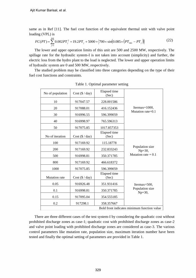
Table 1. Optimal parameter setting

There are three different cases of the test system-I by considering the quadratic cost without

prohibited discharge zones as case-1; quadratic cost with prohibited discharge zones as case-2

and valve point loading with prohibited discharge zones are considered as case-3. The various

control parameters like mutation rate, population size, maximum iteration number have been

tested and finally the optimal setting of parameters are provided in Table 1.

No of population Cost ($ / day) Elapsed time

(Sec)

Itermax=1000,

Mutation rate=0.1

10 917047.57 228.001586

20 917088.01 416.152436

30 916996.55 596.399059

40 916998.97 765.596313

50 917075.85 1017.857353

No of iteration Cost ($ / day)

Elapsed time

(Sec)

Population size

Np=30,

Mutation rate = 0.1

100 917169.92 115.18778

200 917169.92 232.833243

500 916998.81 350.371785

800 917169.92 466.618372

1000 917075.85 596.399059

Mutation rate Cost ($ / day)

Elapsed time

(Sec)

Itermax=500,

Population size

Np=30,

0.05 916926.48 351.931416

0.1 916998.81 350.371785

0.15 917095.04 354.555185

0.2 917298.1 358.357667

Bold front indicates minimum function value


329

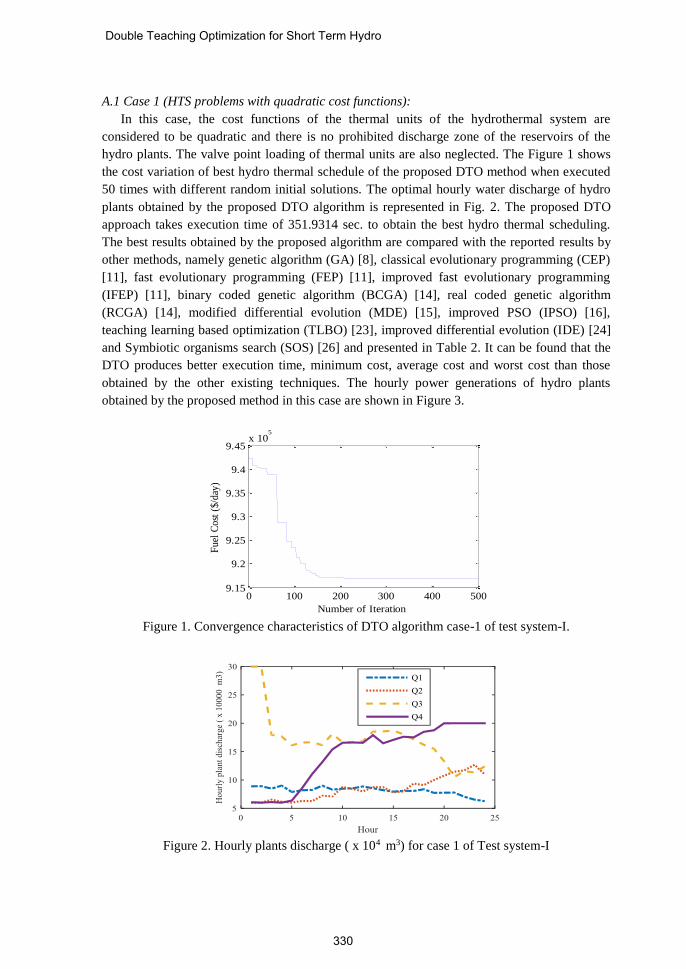
A.1 Case 1 (HTS problems with quadratic cost functions):

In this case, the cost functions of the thermal units of the hydrothermal system are

considered to be quadratic and there is no prohibited discharge zone of the reservoirs of the

hydro plants. The valve point loading of thermal units are also neglected. The Figure 1 shows

the cost variation of best hydro thermal schedule of the proposed DTO method when executed

50 times with different random initial solutions. The optimal hourly water discharge of hydro

plants obtained by the proposed DTO algorithm is represented in Fig. 2. The proposed DTO

approach takes execution time of 351.9314 sec. to obtain the best hydro thermal scheduling.

The best results obtained by the proposed algorithm are compared with the reported results by

other methods, namely genetic algorithm (GA) [8], classical evolutionary programming (CEP)

[11], fast evolutionary programming (FEP) [11], improved fast evolutionary programming

(IFEP) [11], binary coded genetic algorithm (BCGA) [14], real coded genetic algorithm

(RCGA) [14], modified differential evolution (MDE) [15], improved PSO (IPSO) [16],

teaching learning based optimization (TLBO) [23], improved differential evolution (IDE) [24]

and Symbiotic organisms search (SOS) [26] and presented in Table 2. It can be found that the

DTO produces better execution time, minimum cost, average cost and worst cost than those

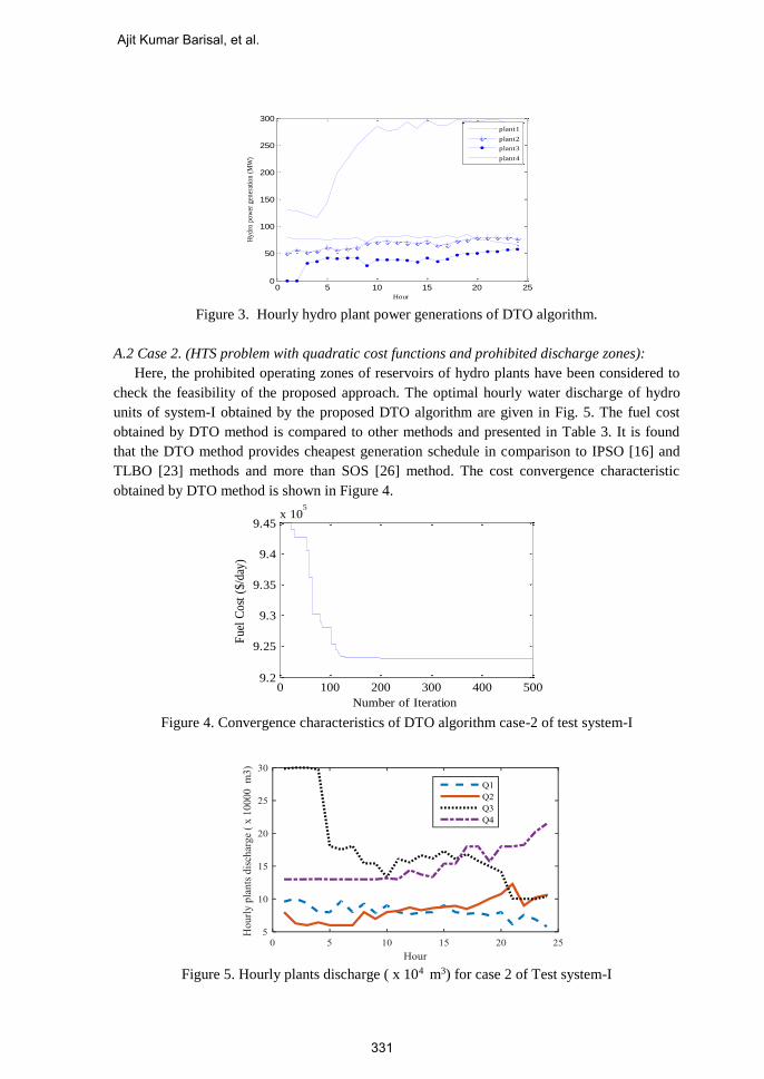
obtained by the other existing techniques. The hourly power generations of hydro plants

obtained by the proposed method in this case are shown in Figure 3.

0 100 200 300 400 5009.15

9.2

9.25

9.3

9.35

9.4

9.45x 10

5

Number of Iteration

Fu

el C

ost

($

/day

)

Figure 1. Convergence characteristics of DTO algorithm case-1 of test system-I.

Figure 2. Hourly plants discharge ( x 104 m3) for case 1 of Test system-I


330

0 5 10 15 20 250

50

100

150

200

250

300

Hour

Hy

dro

po

wer

gen

erat

ion

(M

W)

plant1

plant2

plant3

plant4

Figure 3. Hourly hydro plant power generations of DTO algorithm.

A.2 Case 2. (HTS problem with quadratic cost functions and prohibited discharge zones):

Here, the prohibited operating zones of reservoirs of hydro plants have been considered to

check the feasibility of the proposed approach. The optimal hourly water discharge of hydro

units of system-I obtained by the proposed DTO algorithm are given in Fig. 5. The fuel cost

obtained by DTO method is compared to other methods and presented in Table 3. It is found

that the DTO method provides cheapest generation schedule in comparison to IPSO [16] and

TLBO [23] methods and more than SOS [26] method. The cost convergence characteristic

obtained by DTO method is shown in Figure 4.

0 100 200 300 400 5009.2

9.25

9.3

9.35

9.4

9.45x 10

5

Number of Iteration

Fuel

Cost

($/d

ay)

Figure 4. Convergence characteristics of DTO algorithm case-2 of test system-I

Figure 5. Hourly plants discharge ( x 104 m3) for case 2 of Test system-I


331

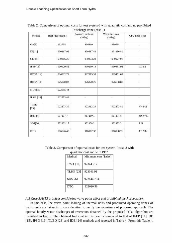
Table 2. Comparison of optimal costs for test system-I with quadratic cost and no prohibited

discharge zone (case 1)

Method Best fuel cost ($) Average fuel cost

($/day)

Worst fuel cost

($/day) CPU time (sec)

GA[8] 932734 936969 939734 -

EP[11] 930267.92 930897.44 931396.81 -

CEP[11] 930166.25 930373.23 930927.01 -

IFEP[11] 930129.82 930290.13 930881.92 1033.2

BCGA[14] 926922.71 927815.35 929451.09 -

RCGA[14] 925940.03 926120.26 926538.81 -

MDE[15] 922555.44 - - -

IPSO [16] 922553.49 - - -

TLBO

[23] 922373.39 922462.24 922873.81 374.918

IDE[24] 917237.7 917250.1 917277.8 366.0781

SOS[26] 922332.17 922338.2 922482.2 6.21

DTO 916926.48 916962.37 916998.76 351.932

Table 3. Comparison of optimal costs for test system-I case-2 with

quadratic cost and with PDZ

Method Minimum cost ($/day)

IPSO [16] 923443.17

TLBO [23] 923041.91

SOS[26] 922844.7835

DTO 923010.56

A.3 Case 3.(HTS problem considering valve point effect and prohibited discharge zone):

In this case, the valve point loading of thermal units and prohibited operating zones of

hydro units are taken in to consideration to verify the robustness of proposed approach. The

optimal hourly water discharges of reservoirs obtained by the proposed DTO algorithm are

furnished in Fig. 6. The obtained fuel cost in this case is compared to that of IFEP [11], DE

[15], IPSO [16], TLBO [23] and IDE [24] methods and reported in Table 4. From this Table 4,


332

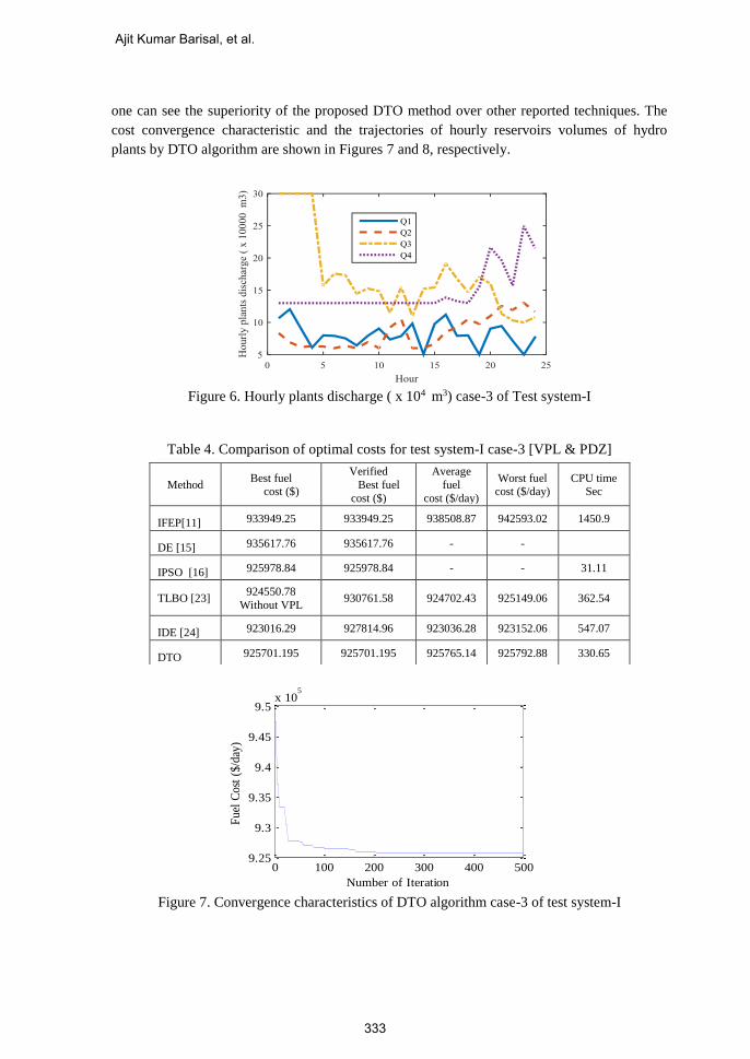
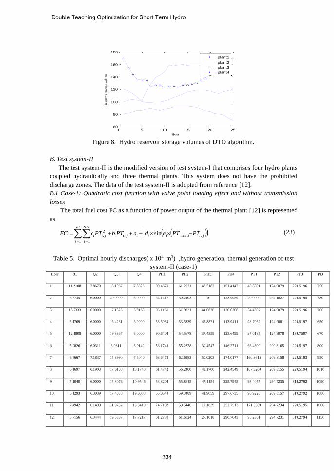
one can see the superiority of the proposed DTO method over other reported techniques. The

cost convergence characteristic and the trajectories of hourly reservoirs volumes of hydro

plants by DTO algorithm are shown in Figures 7 and 8, respectively.

Figure 6. Hourly plants discharge ( x 104 m3) case-3 of Test system-I

Table 4. Comparison of optimal costs for test system-I case-3 [VPL & PDZ]

0 100 200 300 400 5009.25

9.3

9.35

9.4

9.45

9.5x 10

5

Number of Iteration

Fu

el C

ost

($

/day

)

Figure 7. Convergence characteristics of DTO algorithm case-3 of test system-I

Method Best fuel

cost ($)

Verified

Best fuel

cost ($)

Average

fuel

cost ($/day)

Worst fuel cost ($/day)

CPU time Sec

IFEP[11] 933949.25 933949.25 938508.87 942593.02 1450.9

DE [15] 935617.76 935617.76 - -

IPSO [16] 925978.84 925978.84 - - 31.11

TLBO [23] 924550.78

Without VPL 930761.58 924702.43 925149.06 362.54

IDE [24] 923016.29 927814.96 923036.28 923152.06 547.07

DTO 925701.195 925701.195 925765.14 925792.88 330.65


333

0 5 10 15 20 2560

80

100

120

140

160

180

Hour

Res

ervo

ir s

tora

ge v

olum

e

plant1

plant2

plant3

plant4

Figure 8. Hydro reservoir storage volumes of DTO algorithm.

B. Test system-II

The test system-II is the modified version of test system-I that comprises four hydro plants

coupled hydraulically and three thermal plants. This system does not have the prohibited

discharge zones. The data of the test system-II is adopted from reference [12].

B.1 Case-1: Quadratic cost function with valve point loading effect and without transmission

losses

The total fuel cost FC as a function of power output of the thermal plant [12] is represented

as

nt

i

NH

j

jiiiiijiijii PTPTedaPTbPTcFC

1 1

,min,,2, sin (23)

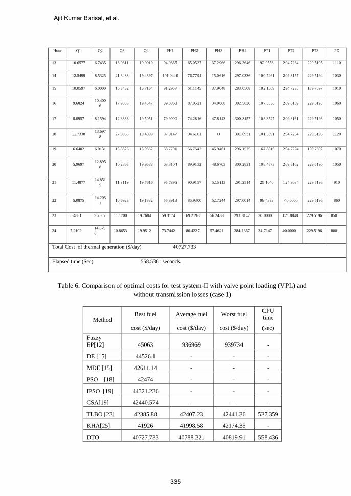
Table 5. Optimal hourly discharges( x 104 m3) ,hydro generation, thermal generation of test

system-II (case-1) Hour Q1 Q2 Q3 Q4 PH1 PH2 PH3 PH4 PT1 PT2 PT3 PD

1 11.2108 7.8670 18.1967 7.8825 90.4679 61.2921 48.5182 151.4142 43.8801 124.9079 229.5196 750

2 6.3735 6.0000 30.0000 6.0000 64.1417 50.2403 0 123.9959 20.0000 292.1027 229.5195 780

3 13.6333 6.0000 17.1328 6.0158 95.1161 51.9231 44.0620 120.0206 34.4507 124.9079 229.5196 700

4 5.1769 6.0000 16.4231 6.0000 53.5039 53.5339 45.8871 113.9411 28.7062 124.9081 229.5197 650

5 12.4808 6.0000 19.3367 6.0000 90.6404 54.5678 37.4559 125.6499 97.0185 124.9078 139.7597 670

6 5.2826 6.0311 6.0311 6.0142 53.1743 55.2828 39.4547 146.2711 66.4809 209.8165 229.5197 800

7 6.5667 7.1837 15.3990 7.5040 63.6472 62.6183 50.0203 174.0177 160.3615 209.8158 229.5193 950

8 6.1697 6.1903 17.6108 13.1740 61.4742 56.2400 43.1700 242.4549 167.3260 209.8155 229.5194 1010

9 5.1040 6.0000 15.8076 10.9546 53.8204 55.8615 47.1154 225.7945 93.4055 294.7235 319.2792 1090

10 5.1293 6.3039 17.4038 19.0088 55.0543 59.3489 41.9059 297.6735 96.9226 209.8157 319.2792 1080

11 7.4942 6.1499 21.9732 13.3410 74.7182 59.5446 17.1839 252.7513 171.5589 294.7234 229.5195 1000

12 5.7156 6.3444 19.5387 17.7217 61.2730 61.6824 27.1018 290.7043 95.2361 294.7231 319.2794 1150


334

Hour Q1 Q2 Q3 Q4 PH1 PH2 PH3 PH4 PT1 PT2 PT3 PD

13 10.6577 6.7435 16.9611 19.0010 94.0865 65.0537 37.2966 296.3646 92.9556 294.7234 229.5195 1110

14 12.5499 8.5325 21.3488 19.4397 101.0440 76.7794 15.0616 297.0336 100.7461 209.8157 229.5194 1030

15 10.0597 6.0000 16.3432 16.7164 91.2957 61.1145 37.9048 283.0508 102.1509 294.7235 139.7597 1010

16 9.6824 10.400

6 17.9833 19.4547 89.3868 87.0521 34.0868 302.5830 107.5556 209.8159 229.5198 1060

17 8.0957 8.1594 12.3838 19.5051 79.9000 74.2816 47.8143 300.3157 108.3527 209.8161 229.5196 1050

18 11.7338 13.697

8 27.9055 19.4099 97.9147 94.6101 0 301.6931 101.5391 294.7234 229.5195 1120

19 6.6402 6.0131 13.3825 18.9552 68.7791 56.7542 45.9461 296.1575 167.8816 294.7224 139.7592 1070

20 5.9697 12.895

8 10.2863 19.9588 63.3104 89.9132 48.6703 300.2831 108.4873 209.8162 229.5196 1050

21 11.4877 14.851

5 11.3119 19.7616 95.7895 90.9157 52.5113 291.2514 25.1040 124.9084 229.5196 910

22 5.0875 14.205

1 10.6923 19.1882 55.3913 85.9300 52.7244 297.0014 99.4333 40.0000 229.5196 860

23 5.4881 9.7507 11.1700 19.7684 59.3174 69.2198 56.2438 293.8147 20.0000 121.8848 229.5196 850

24 7.2102 14.679

6 10.8653 19.9512 73.7442 80.4227 57.4621 284.1367 34.7147 40.0000 229.5196 800

Total Cost of thermal generation ($/day) 40727.733

Elapsed time (Sec) 558.5361 seconds.

Table 6. Comparison of optimal costs for test system-II with valve point loading (VPL) and

without transmission losses (case 1)

Method Best fuel Average fuel Worst fuel

CPU

time

cost ($/day) cost ($/day) cost ($/day) (sec)

Fuzzy

EP[12] 45063 936969 939734 -

DE [15] 44526.1 - - -

MDE [15] 42611.14 - - -

PSO [18] 42474 - - -

IPSO [19] 44321.236 - - -

CSA[19] 42440.574 - - -

TLBO [23] 42385.88 42407.23 42441.36 527.359

KHA[25] 41926 41998.58 42174.35 -

DTO 40727.733 40788.221 40819.91 558.436


335

In this case study the number of decision variable is 168 (4 24 + 3 24) representing the

discharges of four hydro reservoirs and generation of three thermal plants over the entire

scheduling horizon. The optimal hourly discharges obtained by proposed DTO method,

generated powers from hydro and thermal plants over the entire scheduling period are provided

in Table 5. The optimal cost obtained from the proposed DTO based approach have also been

compared with that of EP [12], DE [15], MDE [15], PSO [18], CSA [19], TLBO [23] and

KHA[25]and details are given in Table 6. From the result, it is quite evident that the proposed

DTO based algorithm provides better solution for the cascaded hydro reservoirs with multiple

thermal power plants.

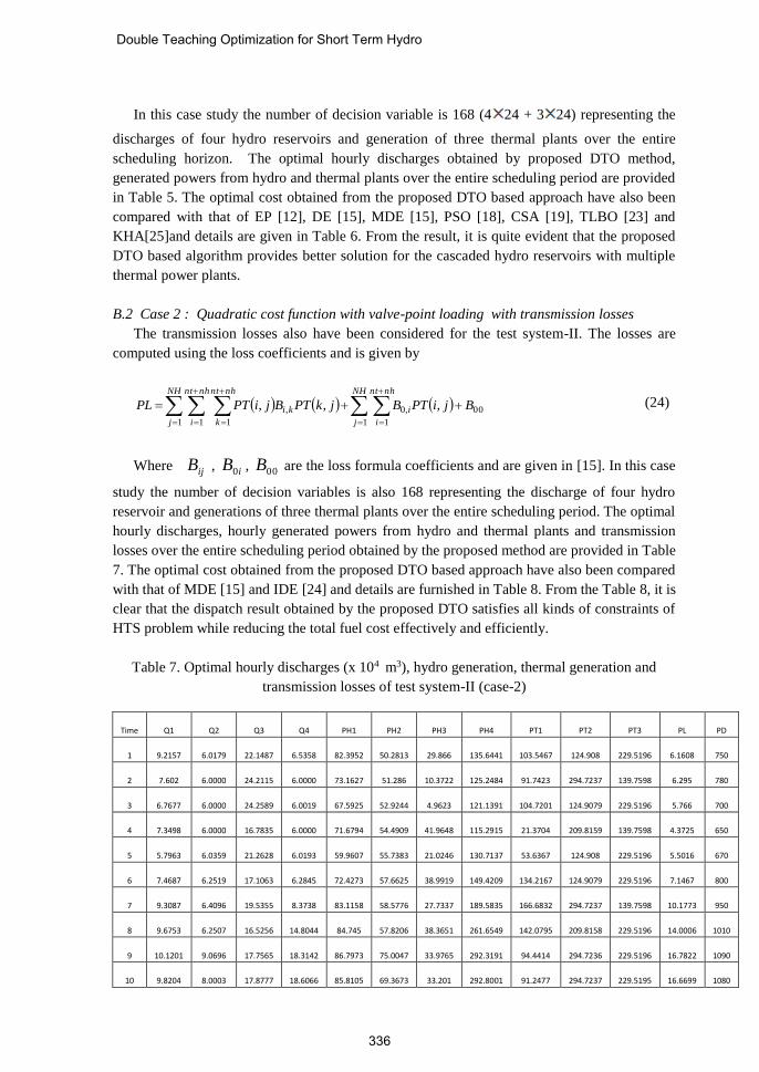
B.2 Case 2 : Quadratic cost function with valve-point loading with transmission losses

The transmission losses also have been considered for the test system-II. The losses are

computed using the loss coefficients and is given by

NH

j

nhnt

i

NH

j

nhnt

i

iki

nhnt

k

BjiPTBjkPTBjiPTPL

1 1

00

1 1

,0,

1

,,, (24)

Where ijB , iB0 , 00B are the loss formula coefficients and are given in [15]. In this case

study the number of decision variables is also 168 representing the discharge of four hydro

reservoir and generations of three thermal plants over the entire scheduling period. The optimal

hourly discharges, hourly generated powers from hydro and thermal plants and transmission

losses over the entire scheduling period obtained by the proposed method are provided in Table

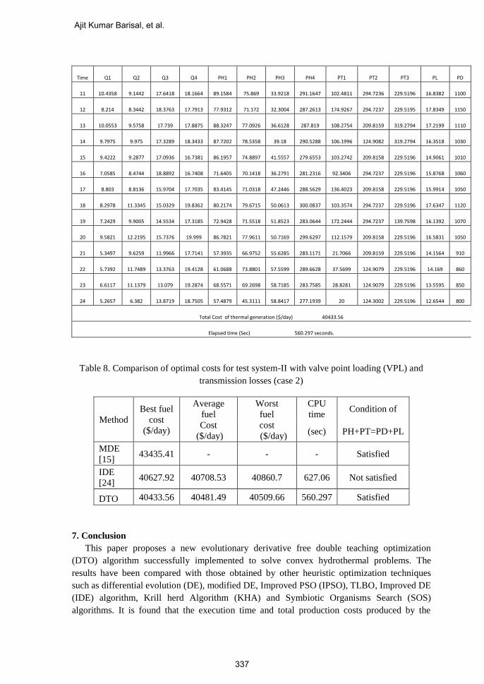
7. The optimal cost obtained from the proposed DTO based approach have also been compared

with that of MDE [15] and IDE [24] and details are furnished in Table 8. From the Table 8, it is

clear that the dispatch result obtained by the proposed DTO satisfies all kinds of constraints of

HTS problem while reducing the total fuel cost effectively and efficiently.

Table 7. Optimal hourly discharges (x 104 m3), hydro generation, thermal generation and

transmission losses of test system-II (case-2)

Time Q1 Q2 Q3 Q4 PH1 PH2 PH3 PH4 PT1 PT2 PT3 PL PD

1 9.2157 6.0179 22.1487 6.5358 82.3952 50.2813 29.866 135.6441 103.5467 124.908 229.5196 6.1608 750

2 7.602 6.0000 24.2115 6.0000 73.1627 51.286 10.3722 125.2484 91.7423 294.7237 139.7598 6.295 780

3 6.7677 6.0000 24.2589 6.0019 67.5925 52.9244 4.9623 121.1391 104.7201 124.9079 229.5196 5.766 700

4 7.3498 6.0000 16.7835 6.0000 71.6794 54.4909 41.9648 115.2915 21.3704 209.8159 139.7598 4.3725 650

5 5.7963 6.0359 21.2628 6.0193 59.9607 55.7383 21.0246 130.7137 53.6367 124.908 229.5196 5.5016 670

6 7.4687 6.2519 17.1063 6.2845 72.4273 57.6625 38.9919 149.4209 134.2167 124.9079 229.5196 7.1467 800

7 9.3087 6.4096 19.5355 8.3738 83.1158 58.5776 27.7337 189.5835 166.6832 294.7237 139.7598 10.1773 950

8 9.6753 6.2507 16.5256 14.8044 84.745 57.8206 38.3651 261.6549 142.0795 209.8158 229.5196 14.0006 1010

9 10.1201 9.0696 17.7565 18.3142 86.7973 75.0047 33.9765 292.3191 94.4414 294.7236 229.5196 16.7822 1090

10 9.8204 8.0003 17.8777 18.6066 85.8105 69.3673 33.201 292.8001 91.2477 294.7237 229.5195 16.6699 1080


336

Time Q1 Q2 Q3 Q4 PH1 PH2 PH3 PH4 PT1 PT2 PT3 PL PD

11 10.4358 9.1442 17.6418 18.1664 89.1584 75.869 33.9218 291.1647 102.4811 294.7236 229.5196 16.8382 1100

12 8.214 8.3442 18.3763 17.7913 77.9312 71.172 32.3004 287.2613 174.9267 294.7237 229.5195 17.8349 1150

13 10.0553 9.5758 17.739 17.8875 88.3247 77.0926 36.6128 287.819 108.2754 209.8159 319.2794 17.2199 1110

14 9.7975 9.975 17.3289 18.3433 87.7202 78.5358 39.18 290.5288 106.1996 124.9082 319.2794 16.3518 1030

15 9.4222 9.2877 17.0936 16.7381 86.1957 74.8897 41.5557 279.6553 103.2742 209.8158 229.5196 14.9061 1010

16 7.0585 8.4744 18.8892 16.7408 71.6405 70.1418 36.2791 281.2316 92.3406 294.7237 229.5196 15.8768 1060

17 8.803 8.8136 15.9704 17.7035 83.4145 71.0318 47.2446 288.5629 136.4023 209.8158 229.5196 15.9914 1050

18 8.2978 11.3345 15.0329 19.8362 80.2174 79.6715 50.0613 300.0837 103.3574 294.7237 229.5196 17.6347 1120

19 7.2429 9.9005 14.5534 17.3185 72.9428 71.5518 51.8523 283.0644 172.2444 294.7237 139.7598 16.1392 1070

20 9.5821 12.2195 15.7376 19.999 86.7821 77.9611 50.7169 299.6297 112.1579 209.8158 229.5196 16.5831 1050

21 5.3497 9.6259 11.9966 17.7141 57.3935 66.9752 55.6285 283.1171 21.7066 209.8159 229.5196 14.1564 910

22 5.7392 11.7489 13.3763 19.4128 61.0688 73.8801 57.5599 289.6628 37.5699 124.9079 229.5196 14.169 860

23 6.6117 11.1379 13.079 19.2874 68.5571 69.2698 58.7185 283.7585 28.8281 124.9079 229.5196 13.5595 850

24 5.2657 6.382 13.8719 18.7505 57.4879 45.3111 58.8417 277.1939 20 124.3002 229.5196 12.6544 800

Total Cost of thermal generation ($/day) 40433.56

Elapsed time (Sec) 560.297 seconds.

Table 8. Comparison of optimal costs for test system-II with valve point loading (VPL) and

transmission losses (case 2)

Method

Best fuel

cost

($/day)

Average

fuel

Cost

($/day)

Worst

fuel

cost

($/day)

CPU

time Condition of

(sec) PH+PT=PD+PL

MDE

[15] 43435.41 - - - Satisfied

IDE

[24] 40627.92 40708.53 40860.7 627.06 Not satisfied

DTO 40433.56 40481.49 40509.66 560.297 Satisfied

7. Conclusion

This paper proposes a new evolutionary derivative free double teaching optimization

(DTO) algorithm successfully implemented to solve convex hydrothermal problems. The

results have been compared with those obtained by other heuristic optimization techniques

such as differential evolution (DE), modified DE, Improved PSO (IPSO), TLBO, Improved DE

(IDE) algorithm, Krill herd Algorithm (KHA) and Symbiotic Organisms Search (SOS)

algorithms. It is found that the execution time and total production costs produced by the


337

proposed DTO method over the scheduling horizon is better or close to other existing

optimization techniques in almost all cases considered in this study.

8. Reference

[1]. J. Wood, B. F. Wollenberg, “Power Generation Operation and Control”, John Wiley

and Sons, New York , 1984.

[2]. M. F. Carvalloh, S. Soares, “An efficient hydrothermal scheduling algorithm,” IEEE

Transactions on Power Systems, Vol. 4, pp. 537-542, 1987.

[3]. J. S. Yang, N. Chen, “Short term hydro thermal coordination using multi-pass dynamic

programming”, IEEE Transactions on Power Systems, Vol. 4, No. 3, pp. 1050-1056,

1989.

[4]. S. Chang, C. Chen, I. Fung, P. B. Luh, “Hydroelectric generation scheduling with an

effective differential dynamic programming”, IEEE Transactions on Power Systems,

Vol. 5, pp.737-743, 1990.

[5]. R. Liang, Y. Hsu, “Scheduling of hydroelectric generation units using artificial neural

networks”, In Generation, Transmission and Distribution, IEE Proceedings, Vol. 141,

No. 5, pp. 452-458, 1994.

[6]. K. P. Wong, Y. W. Wong, “Short term hydrothermal scheduling: part 1. Simulated

annealing approach”, In Generation, Transmission and Distribution, IEE Proceedings,

Vol. 141, No. 5, pp. 497-501, 1994.

[7]. T. Nenad, “A coordinated approach for real-time short term hydro scheduling”, IEEE

Transactions on Power Apparatus System., Vol. 11, No. 4, pp. 1698-704, 1996.

[8]. S. O. Orero, M. R. Irving, “A genetic algorithm modeling framework and solution

technique for short term optimal hydro thermal scheduling”, IEEE Transactions on

Power Systems, Vol. 13, No. 2, pp.501-518, 1998.

[9]. P. K. Hota, R. Chakrabarti, P. K. Chattopadhyay, “Short term hydro thermal Scheduling

through evolutionary technique”, Electric Power Syst. Res., Vol. 52, pp.189-196. 1999.

[10]. R. Naresh, J. Sharma, “Short term hydro scheduling using two phase neural network,”

International Journal of Electrical Power and Energy Systems, Vol. 24, No. 7, pp. 583-

590, 2002.

[11]. N. Sinha, R. Chakrabarti, P. K. Chattopadhyay, “Fast evolutionary technique for short

term hydrothermal scheduling”, IEEE Transactions on Power Systems, Vol. 18, No. 1,

pp. 214-220, 2003.

[12]. M. Basu, “An interactive fuzzy satisfying method based on evolutionary programming

technique for multi-objective short term hydro thermal scheduling”, Electric Power

Systems Research, Vol. 69, No. (2-3), pp. 277-285, 2004.

[13]. M. Basu, “A simulated annealing–based goal attainment method for economic emission

load dispatch of fixed head hydro thermal power system”, International Journal of

Electrical Power and Energy Systems, Vol. 27, No. 2, pp. 147-153, 2005.

[14]. S. Kumar, R. Naresh, “Efficient real coded genetic algorithm to solve the non-convex

hydro thermal scheduling problem”, International Journal of Electrical Power and

Energy Systems, Vol. 29, No. 10, pp. 738-747, 2007.

[15]. L. Lakshminarasimman, S. Subramanian, “Short term scheduling of hydro thermal

power system with cascaded reservoirs by using modified differential evolution”, IEE

Proc Gener. Transm. Distrib. Vol. 153, No. 6, pp. 693-700, 2006.


338

[16]. P. K. Hota, A. K. Barisal, R. Chakrabarti, “An improved PSO technique for short term

optimal hydrothermal scheduling”, Electric Power Systems Research, 79, No. 7, pp.

1047-1053, 2009.

[17]. P. K. Roy, D. Mandal, “Quasi-oppositional biogeography-based optimization for multi-

objective optimal power flow”, Electric Power Components and Systems Vol. 40, No. 2,

pp. 236-256, 2011.

[18]. K. K. Mandal, N. Chakraborty, “Short term combined economic emission scheduling of

hydro thermal system with cascaded reservoir using particle swarm optimization

technique”, Applied Soft Computing, Vol. 11, No. 1, pp. 1295-1302, 2011.

[19]. R. K. Swain, A. K. Barisal, P. K. Hota, R. Chakrabarti, “Short term hydro thermal

scheduling using clonal selection algorithm”, International Journal of Electrical Power

and Energy Systems, Vol. 33 No. 3, pp.647-656, 2011.

[20]. R. V. Rao, V. J. Savsani, D. P. Vakharia, “Teaching- learning based optimization: an

optimization method for continuous non-linear large scale problems”, Information

Sciences, Vol. 183, No. 1, pp. 1-15, 2012.

[21]. X. Liao, J. Zhou, R. Zhang, Y. Zhang, “An adaptive artificial bee colony algorithm for

long term economic dispatch in cascaded hydropower systems”, International Journal

of Electrical Power and Energy Systems, Vol. 43, No. 1, pp. 1340-1345, 2012.

[22]. V. H. Hinojosa, C. Leyton, “Short term hydrothermal generation scheduling solved with

a mixed binary evolutionary particle swarm optimizer”, Electric Power Systems

Research, Vol. 92, pp. 162-170, 2012.

[23]. P. K. Roy, “Teaching learning based optimization for short term hydro thermal

scheduling problem considering valve point effect and prohibited discharge constraint”,

International Journal of Electrical Power and Energy Systems, Vol. 53, pp.10-19, 2013.

[24]. M. Basu, “Improved differential evolution for short term hydro thermal scheduling”,

International Journal of Electrical Power and Energy Systems, Vol. 58, pp. 91-100,

2014.

[25]. Provas Kumar Roy, Moumita Pradhan, Tandra Paul. “Krill herd algorithm applied to

short-term hydrothermal scheduling problem”, Ain Shams Engineering Journal, In

Press, https://doi.org/10.1016/j.asej.2015.09.003,October 2015.

[26]. Sujoy Das, A. Bhattacharya. “Symbiotic organisms search algorithm for short-term

hydrothermal scheduling”, Ain Shams Engineering Journal, In Press,

https://doi.org/10.1016/j.asej.2016.04.002, April 2016.

List of symbols

FC total generation cost

jPT power generation of thermal unit at j time interval.

jiPH , power generation ofthi hydro unit at

thj time interval.

Pg power generations from both thermal and hydro at each time interval.

jPD the load demand at the thj time interval

jPL the transmission loss at the thj time interval.

ia , ib ,

ic , id , ie the fuel cost coefficients of the thi thermal plant.


339

iC ,1, iC ,2

, iC ,3 , iC ,4 , iC ,5

, iC ,6 the power generation coefficients of

thi hydro plant.

jiQ , the water discharge of the

thi hydro plants during the thj time interval.

iQmax, the maximum water discharge rate of the

thi hydro plants

iQmin, the minimum water discharge rate of the

thi hydro plants

jiV , the water storage level in the

thi hydro reservoir at the beginning of the thj time

interval.

1,iV , 25,iV the volume of the thi reservoir at the beginning of 1st and 25th hour.

iVmin,,

iVmax,the minimum and maximum water storage level limit of the

thi hydro reservoir.

jiI , the natural inflow of the

thi reservoir at the thj time interval.

jiS , Spillage discharge rate of the

thi reservoir at the thj time interval.

Water delay time between reservoir i and its up-stream u at interval j .

uR Set of upstream units directly above hydro-plant i .

nh

number of hydro unit

nt

number of thermal unit

NH

number of time interval

Np number of population

k

jiX ,,

1

,

k

jiX the grade of the thj subject of the

thi student at the thk and

thk )1( iteration

k

diffj the difference between the mean of thethj control variable at the

thk and

thk )1( iteration.

rand random number between [0,1]


340

Ajit Kumar Barisal received the B.E. degree from the U.C.E, Burla (now

VSSUT), Odisha, India in 1998 and the M.Tech degree in power system

from Bengal engineering College (now IIEST), Shibpur, Howrah, in 2001

and Ph. D degree from Jadavpur University, Kolkata in 2010, in electrical

engineering. He was with the Electrical Engineering Department, NIST,

Berhampur, Odisha, from 2000 to 2004 and with Electrical and Electronics

Engineering Department, Silicon Institute of Technology, Bhubaneswar,

Odisha, from 2004 to 2005. He is associated in the Department of Electrical

Engineering, V.S.S University of Technology, Burla, Odisha Since 2006 as Associate

Professor. He received the “Odisha Young Scientist award- 2010”, IEI Young Engineers

award- 2010” and “Union Ministry of Power, Department of power prize- 2010” for his

outstanding contribution to Engineering and Technology research. His research interests

include economic load dispatch, Hydrothermal Scheduling, alternative energy power

generation, AGC and soft computing applications to different power system problems.

Ramesh Chandra Pusty born in 1982 and received the B. Tech. Degree

from the NIST, Berhampur, Odisha, in 2006 and M. Tech. degree in power

system engineering in the Electrical Engineering Department, V.S.S

University of Technology, Burla, Odisha, India. He was working as Asst

Professor in Electrical Engineering Department, Maharaja Institute of

Technology, Bhubaneswar, Odisha, from 2010 to 2011. Since 2011, he is

working as Assistant professor in the Electrical Engineering Department,

V.S.S University of Technology, Burla, Odisha, India. His research interests

include Hydrothermal Scheduling and soft computing applications to power system problems.

Kumadini Suna received the B.Tech. degree from the Indira Gandhi

Institute of Technology, Sarang, Odisha, India in 2012 and the M.Tech

degree in power system Engineering from Veer Surendra Sai University of

Technology, Burla, Odisha, India, in 2014, in Electrical Engineering...

Presently, she is working Assistant Executive Engineer at Department of

Energy, Govt of Odisha, India. She has published few papers in different

reputed journals in her credit. Her interest area is soft computing applications

in Power system.

Tapas Kumar Panigrahi received the B.E. degree from the U.C.E, Burla

(now VSSUT), Odisha, India in 1993 and the M.Tech degree in power

system from Bengal engineering College (now IIEST), Shibpur, Howrah, in

2001 and Ph. D degree from Sambalpur University, Burla, Odisha in 2015, in

electrical engineering.. He is presently working as an Asst. Professor in the

Department of Electrical and Electronics Engineering, I.I.I.T, Bhubaneswar,

Odisha, India. He has published more than 20 papers in different reputed

international journals in his credit. His interest area is soft computing

applications in Power system, AGC, Renewable Energy Systems and Micro-grid.


341

double teaching optimization for short term hydro thermal...

Documents