does advertising overcome brand loyalty? evidence...

Does Advertising Overcome BrandLoyalty? Evidence from theBreakfast-Cereals Market

MATTHEW SHUM

Johns Hopkins UniversityBaltimore, MD 21218

[email protected]

In differentiated product markets where consumer preferences are characterizedby brand loyalty, an important role for advertising may be to overcome brandloyalty by encouraging consumers to switch to less familiar brands. Using ascanner panel dataset of breakfast-cereal purchases, I find evidence consistentwith the hypothesis that advertising counteracts the tendencies of brand loyaltytoward repeat purchasing. Equivalently, advertising reduces switching costsin this market. Furthermore, counterfactual experiments demonstrate that inmarkets with brand loyalty, advertising is an attractive and effective option—relative to alternative promotional activities, such as price discounts—ofstimulating demand for a brand.

1. Introduction

Brand loyalty in consumer preferences can be a significant source ofincumbent advantage in many differentiated product markets because itbuilds up switching costs, which makes consumers reluctant to try newbrands. In these markets, a potentially important role for advertisingmay be to counteract the tendencies of brand loyalty by encouragingconsumers to “switch” to newer, less familiar brands.

This consideration goes against the grain of an argument datingback to Bain (1956) and Comanor and Wilson (1974) (hereafter B/CW)that advertising fosters perceived product differentiation among other-wise very similar brands. For example, Bain (1956) wrote that “product

I am grateful to James Lattin (Stanford GSB) and Ronald Cotterill (University of Connecti-cut Food Marketing Policy Center) for providing me with the data used in this paper.I thank the editor, Dan Spulber, as well as a coeditor and two referees, for their carefulreading and suggestions on previous drafts. I also thank Anand Bodapati, Tim Bresnahan,Andrea Coscelli, Greg Crawford, Nancy Gallini, Amil Petrin, Rob Porter, Peter Reiss,Frank Wolak, and participants in the NBER Summer Institute 1999 for their commentsand advice.

c© 2004 Blackwell Publishing, 350 Main Street, Malden, MA 02148, USA, and 9600 Garsington Road,Oxford OX4 2DQ, UK.Journal of Economics & Management Strategy, Volume 13, Number 2, Summer 2004, 241–272

242 Journal of Economics & Management Strategy

differentiation is propagated by [. . .] advertising and sales-promotionalefforts designed to win the allegiance and custom of the potential buyer”(p. 114).

But Shapiro (1982) countered that

[CW] correctly identify brand loyalty [. . .] as the critical issue[. . .] in markets of the type they are looking at, i.e., whereadvertising is important. The problem arises when they tryto attribute brand loyalty to advertising expenditures alone.A very different conclusion emerges if brand loyalty is at-tributed instead to . . . consumer experience, with advertisingbeing a method of overcoming brand loyalty (p. 6).

In this paper I evaluate the validity of Shapiro’s (1982) argumentfor the breakfast-cereals industry by investigating whether advertisingreduces brand loyalty in this market. This market appears, at first glance,to be a textbook case of the B/CW argument. The advertising intensityof the breakfast-cereals market is extraordinarily high: The advertising-to-sales ratio for the Grain Mills Products industry [Standard industrialclassification (SIC) 2040, the bulk of which is cereals] is about 1.2 timesthe average value for the food sector and is about 3.5 times higher thanthe average value for all industrial sectors.1 At the same time, thereare a very large number of brands of cereals available at any one time(218 distinct brands appear in my dataset). These two characteristicsof the industry—high advertising intensity, and substantial productdifferentiation—by themselves tend to justify the traditional B/CWarguments that advertising sustains perceived product differentiationamong the competing brands.

One potential explanation for these trends is provided in theliterature on advertising’s role in informing consumers, either directly(cf. Butters, 1977; Grossman and Shapiro, 1984; Stigler, 1964) or indirectly(via “signaling”; cf. Kihlstrom and Riordan, 1984; Milgrom and Roberts,1986; Nelson, 1974) about brand attributes and/or prices. These mod-els, however, may have a difficult time explaining cereal advertising,since it is the well-established brands such as General Mills’ Cheeriosor Kellogg’s Frosted Flakes that are the most advertised. Motivatedby Shapiro’s remark, I consider an alternative interpretation of theseadvertising trends: If consumers’ preferences are characterized by brandloyalty, advertising—even for as well-known a brand as Cheerios—must

1. These figures are derived from the Advertising Ratios and Budgets publication ofSchonfeld and Associates.

Does Advertising Overcome Brand Loyalty? 243

be maintained in order to convince consumers loyal to rival brands toswitch.2

The concept of brand loyalty is connected closely to that ofswitching costs so that the question of whether advertising overcomesbrand loyalty is analogous to one regarding whether advertising reducesswitching costs. Therefore, this paper complements a large theoreticalliterature on the competitive effects of switching costs in oligopolisticindustries (see, for example, Klemperer 1984, 1985), as well as a morerecent empirical literature measuring the extent of switching costs inspecific markets [see Chen and Hitt (2001) for a study of online broker-ages, and Stango (2002) for an examination of credit card markets].

In this paper, I employ a scanner panel dataset to estimatehousehold-level cereal brand-choice models in which advertising’s ef-fects depend on a household’s brand loyalty, as measured by its recentpurchases of particular brands. The results enable me to quantify howmuch advertising for a given brand reduces the (implicit) switchingcosts that households incur in trying a brand they have not purchasedrecently.

In the next section I describe some of the existing literature onthis subject and introduce my dataset. In Section 3, I present the cerealbrand-choice model used in this analysis and discuss important specifi-cation and identification issues. Section 4 contains the estimation resultsand discussion thereof. Section 5 reports results from counterfactualexperiments that examine the market-level implications of my findings.Section 6 concludes.

2. Background: Existing Literatureand Data Description

While brand loyalty is a standard component of many brand-choicemodels [especially in the empirical marketing literature, cf. the seminalpaper by Guadagni and Little (1983)], I believe that this paper is the firstto examine its market-level consequences, as well as the implications ofadvertising that potentially reduce brand loyalty. Several recent papersexplore the degree of market power and product differentiation inthe breakfast-cereals market (cf. Cotterill and Haller, 1997; Hausman,

2. Indeed, the New York Times has reported a remark by a marketing director forPhilip Morris’ Polish operations that “I can do much more about switching of brand (sic)[than whether a person smokes or not]. . .” (p. A1). While the physically addictive natureof cigarettes potentially intensifies brand loyalty in that market in a manner differentfrom the cereals market, this statement illustrates the importance that marketers attach toadvertising’s role in promoting switching behavior.


1996; Kiser, 1998; Nevo, 2001). These papers do not focus on the roleof advertising in the breakfast cereals market, or on its effects on thedynamics of purchase decisions.

The closest antecedent to my work is Ackerberg (2001), whoreports strong evidence of advertising’s disproportionately larger effectson households who previously have not purchased a brand. He uses ascanner dataset for the yogurt market, which includes detailed advertis-ing exposure data gleaned from television viewing logs. Furthermore,by focusing on the case of the entry of a new brand of yogurt, Ackerbergcan attribute the differential effects of advertising between householdswho have and have not purchased recently the brand to informationaleffects. Since such an interpretation would not be as appropriate for thecereals market, where the established brands maintain high advertisinglevels, I avoid all informational interpretation of the findings in thispaper.3 However, the essential empirical design in this paper is thesame as Ackerberg’s paper: Households are separated into two groups,depending on whether or not they have purchased recently a givenbrand. The effect of advertising on a household’s purchases of this brandare assumed to differ across these two groups, where the hypothesis ofinterest—that advertising overcomes brand loyalty—implies that ad-vertising should have larger effects on the purchases of the householdswho have not purchased recently the brand.

2.1 Data Description

I employ a detailed household-level scanner dataset [collected by Infor-mation Resources, Inc. (IRI)], which tracks the cereal purchases of 1,010households in six supermarkets in the Chicago metropolitan area on aweekly basis from June 1991 to December 1992.4

As any even casual observer of the cereal markets is aware,there are a large number of breakfast-cereal brands available to theconsumer: In my dataset, around 110 brands of cereals were found in thesupermarket cereal aisle during the average week and, for each of thesebrands, at least two box sizes typically were available. Due to the largenumber of brands, I aggregate up to the top 50 brands in my dataset

3. See also Deighton, Henderson, and Neslin (1994). The question of how advertisingencourages switching is beyond the scope of this paper. Psychological hypotheses thatposit that advertising “cues” or reminds consumers of past experiences may be plausiblein this market, especially given the large number of competing cereal brands. Alba,Hutchinson, and Lynch (1991) contains a general description of this literature.

4. This data were recorded by scanners at the supermarket checkout counters andconstitutes a (small) part of a unique multicategory market basket database in the StanfordBusiness School. See Bell and Lattin (1998) for additional details.


and combine all the other brands into a composite 51st brand.5 Sincemy focus is on brand choice, I aggregate across all different box sizes indefining each brand so that I do not distinguish between, for example,12-ounce. and 20-ounce. boxes of Shredded Wheat. On the other hand,“umbrella extensions” of a brand name are classified as distinct brandsso that, for example, Cheerios and Honey-Nut Cheerios are classified astwo distinct brands. This aggregation procedure resembles that used inHausman (1996) and Nevo (2001).

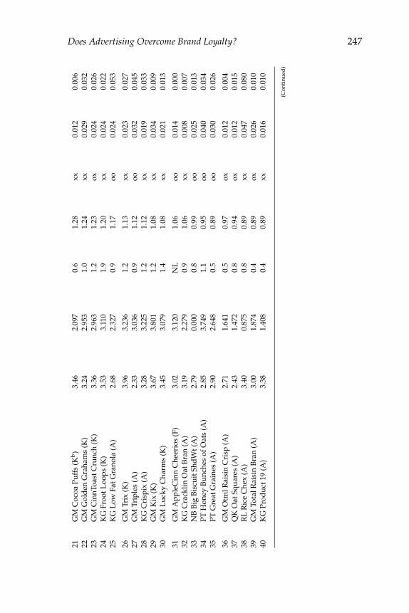
Table I presents summary characteristics for the 51 brands ofcereals used in my analysis. The top-50 brands accounted for just over75% of all purchases in my data. Comparing columns 5 and 6 of Table Ishows that in-sample market shares (calculated from purchases in mydataset) are very close to national market shares. I classify the top-50brands into family (13 brands), adult (25 brands), and kids’ (12 brands)segments, taking as a guide the classification scheme in Hausman (1996).

Column 6 shows that more than half of the top 50 brands existedprior to 1983. Five entered between 1983 and 1988, and 13 after 1988.Furthermore, IRI’s 1995 Marketing Fact Book indicates that 49 of the top-50brands (the sole exception being Quaker’s Popeye brand) still existed in1995. Therefore, while there is substantial product entry into and exit outof the cereals market,6 the set of top-selling cereals has remained quitestable over long periods of time. The third column in Table I summarizesthe average transaction prices for each brand.7 A given brand’s pricevaries across both stores and weeks.

The main advertising data employed in this analysis are quarterlyaggregate (i.e., national) brand-level advertising expenditures data fromleading national advertisers (LNA). Column 5 of Table I presents across-time averages of quarterly advertising expenditures for each brand.The most highly advertised brands are well-established brands, suchas Cheerios and Frosted Flakes. Family cereals are advertised the mostbut are cheaper than both adult and kids’ cereals. While the advertisingnumbers include expenditures on 10 media, almost all of the advertisingdollars were spent on broadcast television advertising, including bothnational and local television.

5. Since stores vary in the nontop-50 brands they carry, the composition of this 51stbrand therefore varies across households as well as over time, depending on in whichstores the households choose to shop.

6. Hausman (1996) notes that from 1980 to 1992, approximately 190 new brands wereintroduced on a basis of about 160 existing brands.

7. On average, the transactions prices (which are computed net of consumers’ couponsavings) are markedly lower than the shelf prices, on an order exceeding 10%. While mostof the results I present here were obtained using transactions prices, I also have estimatedthe model using shelf prices to gauge the robustness of the results.


Tab

le

I.

Br

an

dC

har

acte

ris

tics

Ave

rage

Nat

iona

lSa

mpl

eE

xist

inTr

ansa

ctio

nA

vera

geM

arke

tM

arke

t19

83?

Nam

ePr

ice

($/

lb)

Ad

Exp

ense

cSh

ared

Shar

eeIn

1988

?fFe

atur

egD

ispl

ayh

1K

Ga

Cor

nFl

akes

(Fb)

1.81

7.10

95.

15.

67xx

0.04

00.

058

2G

Ma

Che

erio

s(F

)3.

167.

287

4.8

4.38

xx0.

038

0.04

33

KG

Ric

eK

risp

ies

(F)

2.96

6.03

43.

84.

04xx

0.03

90.

057

4K

GFr

oste

dFl

akes

(F)

2.52

7.86

74.

53.

82xx

0.01

90.

023

5K

GR

aisi

nB

ran

(F)

2.34

5.59

13.

22.

73xx

0.03

40.

045

6G

MTo

tal(

Ab)

3.61

3.92

61.

82.

36xx

0.01

70.

015

7G

MH

oney

Nut

Che

erio

s(F

)3.

144.

030

2.7

2.26

xx0.

016

0.01

78

KG

Spec

ialK

(A)

3.48

3.53

11.

32.

16xx

0.00

00.

000

9PT

aG

rape

Nut

s(A

)2.

146.

740

2.9

2.12

xx0.

001

0.00

110

NB

Spoo

nSiz

eSh

dW

t(A

)2.

810.

025

1.2

2.08

xx0.

035

0.00

2

11Q

Ka

100%

Nat

ural

(A)

2.24

1.61

21.

01.

96ox

0.01

10.

009

12K

GFr

oste

dM

iniW

heat

s(A

)2.

626.

106

2.8

1.84

xx0.

015

0.00

913

KG

Nut

riG

rain

(A)

2.87

2.50

80.

81.

55xx

0.01

20.

011

14K

GM

uesl

ix(A

)3.

311.

975

0.8

1.53

oo0.

017

0.01

615

GM

Whe

atie

s(F

)2.

552.

257

1.4

1.52

xx0.

056

0.15

7

16PT

Rai

sin

Bra

n(F

)2.

234.

361

1.9

1.46

xx0.

041

0.06

217

RL

aM

uesl

i(A

)3.

340.

215

0.4

1.26

oo0.

019

0.01

618

KG

Cor

nPo

ps(F

)3.

513.

198

1.0

1.46

xx0.

023

0.01

919

GM

Rai

sin

Nut

Bra

n(A

)2.

981.

659

1.1

1.35

ox0.

011

0.00

720

GM

Bas

ic4

(A)

3.27

2.51

00.

81.

31oo

0.02

20.

019


21G

MC

ocoa

Puff

s(K

b)

3.46

2.09

70.

61.

28xx

0.01

20.

006

22G

MG

old

enG

raha

ms

(K)

3.24

2.95

31.

01.

24xx

0.02

90.

032

23G

MC

innT

oast

Cru

nch

(K)

3.36

2.96

31.

21.

23ox

0.02

40.

026

24K

GFr

ootL

oops

(K)

3.53

3.11

01.

91.

20xx

0.02

40.

022

25K

GL

owFa

tGra

nola

(A)

2.68

2.32

70.

91.

17oo

0.02

40.

053

26G

MTr

ix(K

)3.

963.

236

1.2

1.13

xx0.

023

0.02

727

GM

Trip

les

(A)

2.33

3.03

60.

91.

12oo

0.03

20.

045

28K

GC

risp

ix(A

)3.

283.

225

1.2

1.12

xx0.

019

0.03

329

GM

Kix

(K)

3.67

3.80

11.

21.

08xx

0.03

40.

009

30G

ML

ucky

Cha

rms

(K)

3.45

3.07

91.

41.

08xx

0.02

10.

013

31G

MA

pple

Cin

nC

heer

ios

(F)

3.02

3.12

0N

L1.

06oo

0.01

40.

000

32K

GC

rack

linO

atB

ran

(A)

3.19

2.27

90.

91.

06xx

0.00

80.

007

33N

BB

igB

iscu

itSh

dW

t(A

)2.

790.

000

0.8

0.99

oo0.

025

0.01

334

PTH

oney

Bun

ches

ofO

ats

(A)

2.85

3.74

91.

10.

95oo

0.04

00.

034

35PT

Gre

atG

rain

es(A

)2.

902.

648

0.5

0.89

oo0.

030

0.02

6

36G

MO

tmlR

aisi

nC

risp

(A)

2.71

1.64

10.

50.

97ox

0.01

20.

004

37Q

KO

atSq

uare

s(A

)2.

431.

472

0.8

0.94

ox0.

012

0.01

538

RL

Ric

eC

hex

(A)

3.40

0.87

50.

80.

89xx

0.04

70.

080

39G

MTo

talR

aisi

nB

ran

(A)

3.00

1.87

40.

40.

89ox

0.02

60.

010

40K

GPr

oduc

t19

(A)

3.38

1.40

80.

40.

89xx

0.01

60.

010

(Con

tinu

ed)


Tab

le

I.

Co

nti

nu

ed

Ave

rage

Nat

iona

lSa

mpl

eE

xist

inTr

ansa

ctio

nA

vera

geM

arke

tM

arke

t19

83?

Nam

ePr

ice

($/

lb)

Ad

Exp

ense

cSh

ared

Shar

eeIn

1988

?fFe

atur

egD

ispl

ayh

41K

GA

pple

Jack

s(K

)3.

641.

465

0.7

0.84

xx0.

030

0.02

342

QK

Cap

tCru

nch

(K)

2.55

1.71

41.

80.

83xx

0.05

20.

066

43N

BSh

red

ded

Whe

at(A

)2.

822.

925

0.5

0.80

xx0.

021

0.00

044

PTFr

uity

Pebb

les

(K)

3.21

1.71

00.

80.

83xx

0.04

00.

040

45G

MC

lust

ers

(F)

3.14

1.42

50.

90.

78ox

0.01

90.

002

46K

GC

inna

mon

Min

iBun

s(F

)2.

750.

002

0.8

0.76

oo0.

029

0.04

347

KG

Dou

ble

Dip

Cru

nch

(A)

3.01

1.45

40.

60.

73oo

0.02

20.

034

48G

MM

ulti

Gra

inC

heer

ios

(F)

3.34

2.52

0N

L0.

75oo

0.03

90.

018

49PT

Hon

eyco

mb

(K)

3.40

2.56

70.

70.

74xx

0.02

20.

023

50Q

KPo

peye

(K)

1.77

0.00

0N

L0.

67oo

0.00

10.

004

51B

aske

tofA

llO

ther

Bra

nds

2.68

0.64

534

.324

.29

0.44

10.

627

a KG

:Kel

logg

s;G

M:G

ener

alM

ills;

PT:P

ost(

Phill

ipM

orri

s);R

L:R

alst

on;Q

K:Q

uake

rO

ats.

bF:

fam

ilyse

gmen

t;A

:ad

ults

egm

ent;

K:k

ids’

segm

ent.

c Qua

rter

lyex

pns,

$mill

.Sou

rce:

Lea

din

gN

atio

nalA

dve

rtis

ers

(199

0–19

93).

Avg

.199

1:ii—

1993

:ii.

dSh

ares

ofna

tion

alce

real

volu

me,

1992

.Sou

rce:

IRI.

NL

:Bra

ndno

tlis

ted

inso

urce

.e S

hare

ofto

tali

n-sa

mpl

epu

rcha

ses.

Sour

ce:A

utho

r’s

calc

ulat

ions

.f x

x:ex

isti

nbo

thye

ars;

ox:e

xist

in19

88,n

otin

1983

;oo:

exis

tin

neit

her

year

.Sou

rce:

IRI.

g=1

ifbr

and

was

feat

ured

inne

wsp

aper

add

urin

ga

give

n(s

tore

-wee

k);a

vg.o

ver

823

stor

ew

eeks

.h=1

ifbr

and

had

feat

ure

dis

play

inst

ore

dur

ing

agi

ven

(sto

re-w

eek)

;avg

.ove

r82

3st

ore

wee

ks.

i Sum

ofav

erag

equ

arte

rly

adve

rtis

ing

expe

ndit

ure

for

allt

heno

ntop

-50

bran

ds.


Table II.

Household Data: Summary Statistics

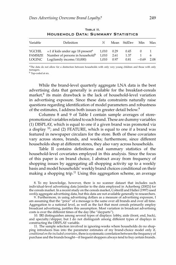
Variable Definition N Mean StdDev Min Max

YGCHIL =1 if kids under age 18 presenta 1,010 0.29 0.45 0 1FAMSIZE Number of persons in householdb 1,010 2.61 1.37 1 6LOGINC Log(family income/10,000) 1,010 0.97 0.81 −0.69 2.08

aThe data do not allow for a distinction between households with only very young children and those with onlyteenagers.b Top-coded at six.

While the brand-level quarterly aggregate LNA data is the bestadvertising data that generally is available for the breakfast-cerealsmarket,8 its main drawback is the lack of household-level variationin advertising exposure. Since these data constraints naturally raisequestions regarding identification of model parameters and robustnessof the estimates, I address both issues in greater detail below.9

Columns 8 and 9 of Table I contain sample averages of store-promotional variables related to each brand. These are dummy variables(1) DISPLAY, which is equal to one if a given brand was promoted viaa display 10; and (2) FEATURE, which is equal to one if a brand wasfeatured in newspaper circulars for the store. Both of these covariatesvary across stores, brands, and weeks; furthermore, since differenthouseholds shop at different stores, they also vary across households.

Table II contains definitions and summary statistics of thehousehold-level covariates employed in this analysis. Since the focusof this paper is on brand choice, I abstract away from frequency ofshopping issues by aggregating all shopping activity up to a weeklybasis and model households’ weekly brand choices conditional on theirmaking a shopping trip.11 Using this aggregation scheme, an average

8. To my knowledge, however, there is no scanner dataset that includes suchindividual-level advertising data [similar to the data employed in Ackerberg (2002)] forthe cereals market. In a recent study on the cereals market, Cotterill and Haller (1997) usedweekly aggregate advertising data, but this data are not available generally to researchers.

9. Furthermore, in using advertising dollars as a measure of advertising exposure, Iam assuming that the “price” of a message is the same over all brands and over all time.Aggregation to a national level, as well as the fact that most cereals primarily employbroadcast advertising, justifies this assumption. Most variation in broadcast advertisingcosts is over the different times of the day (the “dayparts”).

10. IRI distinguishes among several types of displays: lobby, aisle (front, end, back),and specialty/shipper, but I do not distinguish among different types of displays inconstructing the DISPLAY variable.

11. The sample selection involved in ignoring-weeks where households do no shop-ping introduces bias into the parameter estimates of my brand-choice model only if,conditional on the included covariates, there is systematic correlation between the frequency ofpurchase and the brands bought—if frequent shoppers always tend to buy certain brands.


household made a shopping trip during 39.14 out of the 52 weeks in thesample and purchased cereal during 10.36 weeks. There are weeks in thesample in which a household makes multiple purchases, i.e., purchasesof more than a single brand. In the empirical specifications, I model eachof these within-week purchases as independent events.12

Comparison of the demographics and cereal-purchase frequenciesfrom the scanner data used in this study with the Consumer ExpenditureSurvey (a representative consumption survey sample of US householdscollected by the Bureau of Labor Statistics) shows that the households inmy dataset tend to be older than the average US household.13 Further-more, a comparison of cereal purchases suggests that there might be asubstantial incidence of missing purchases in the scanner dataset (aris-ing from households purchasing cereal at nonscanner equipped stores).While these problems do not affect the interpretation of the individual-level results, they are controlled for in the aggregate-level counterfactualexperiments by introducing appropriate household weights, whichcalibrate each sample household according to its representativeness inthe US population.

I measure brand loyalty by households’ past purchases. Specifi-cally, I construct an indicator variable PASTUSEiht, which is equal toone if household h bought brand i in the w weeks preceding purchaseoccasion t.14 The empirical results reported in this paper were obtained

Since the covariates include family size, I believe I have controlled for the most potentiallyimportant source of this type of correlation: households with kids who purchase cerealmost often and whose purchases tend toward kids’ cereals.

12. Households purchased more than one brand in roughly one-quarter of all(household-weeks) in which purchase occurred. By ignoring the multiple purchasedimension, I may be abstracting away from important across-brand synergies that maycharacterize preferences in this market. However, some auxiliary calculations failed tofind signs of across-brand synergies in demand patterns that would require modelingthe multipurchase decision. In particular, I looked for signs of a likely type of demandsynergy: that families with children may tend to buy “bundles” of adult and kids’ cerealsversus one single brand. I found no evidence of this. See Hendel (1999) and Dube (1999)for an extension and applications of the discrete-choice demand framework to handlemultiple choices.

13. Apparently IRI included more older households in their sample because theysought households they deemed to have a low probability of moving out of the samplearea. I thank Anand Bodapati for this insight.

14. An alternative approach would be to allow loyalty to be a “stock” that fadesover time [as in many marketing brand-choice models, starting with Guadagni andLittle (1983)]. However, initial conditions pose nontrivial problems in these models, asdoes determining the appropriate “decay rate” for the experience stock. Moreover, thepossibility of unobserved purchases (as discussed previously) leads to measurementerror in the PASTUSE variable. In earlier versions of this paper, I included results fromspecifications that controlled for this measurement error by explicitly parameterizing theprobability of unobserved purchases as a function of household and brand characteristics.Since the model became quite cumbersome computationally without yielding noticeablydifferent results, I have not included them here.


Table III.

Switch Propensities in theRaw Dataseta

w %SWITCH NumObs

2 82.7 223634 70.8 219468 57.6 2113612 50.5 2020024 38.5 17560

aComputed using all purchases of a top-50 brand in my sample.

from models that assume w = 12.15 In Table III, I compute how oftenhouseholds in my dataset “switched” to brands they had not purchasedrecently. The “%SWITCH” column gives the percentage of observedpurchases that represents purchases of brands a household did notpurchase in the most recent w weeks, for different values of w. Forw = 12, households switched 50.5% of the time.

The dataset employed in my analysis includes the observationsfrom January–December 1992, totaling 44.224 observations. The obser-vations from June–December 1991 were used to initialize the loyaltyvariable PASTUSE.

As a first glimpse of the main empirical exercise undertaken inthis paper—quantifying the differences in advertising’s effects acrosshouseholds that are and are not loyal to a given brand—I aggregatethe purchases of each brand across all households up to the quarterlylevel (the same frequency as the advertising data) and examine theacross-(brand/quarter) correlations between advertising levels and theproportion of purchases of each brand undertaken by households whoare not “loyal” to it (where loyalty is measured with the PASTUSEvariable, for both w = 12 and w = 4). As Table IV shows, results fromlinear regressions (both with and without brand fixed effects to controlfor brand-specific unobservables) indicate positive correlation for bothw = 12 and w = 4. However, not all of these effects are statisticallysignificant (the 12-week effect without brand-fixed effects is significantat the 13% level, and the four-week effect with brand effects is onlysignificant at a 20% level). Moreover, while this positive correlation isconsistent with the hypothesis that advertising encourages switchingbehavior, one cannot adopt this causal interpretation based on thesecorrelations alone. For these reasons, I next examine results from brandchoice models.

15. I also estimated a specification assuming w = 4 as a robustness check. Since theresults did not change much relative to the reported results, I do not consider them here.


Table IV.

Advertising and Switching:Correlations from Raw Dataseta

Loyalty Measure 12 Weeks 4 Weeks

Without Brand-Fixed Effects 0.0068 0.0154(0.0045) (0.0040)

With Brand-Fixed Effectsb 0.01524 0.0072(0.0072) (0.0057)

aSlope coefficients from a linear regression ofNOT L OYit

T OT PU RCiton NADVit . NOTLOYit :

quarter t purchases of brand i by non-loyal households; TOTPURCit : total quarter tpurchases of brand i; and NADVit : quarter t national advertising for brand i. Loyalty ismeasured over both a 12- and a 4-week period. Standard errors in parentheses. Computedusing all purchases of a top-50 brand in my sample.bExcluded brand is brand 50.

3. Empirical Model

Following much of the existing empirical literature on brand choice, Iderive the expressions for the purchase probabilities from a discrete-choice model of household-level brand choice. On each purchase occa-sion, household h chooses among I = 50 cereal brands. In addition, it canchoose to purchase no brand of cereal at all: This is denoted option “0”.Household h chooses the alternative i(i = 0, . . . , 50), which provides thehighest indirect utility:

maxi∈[0,...,50]

Uiht. (1)

Taking a random-utility approach, I assume that the utility Uiht =Viht + ηiht, where Viht is a deterministic component and ηiht a randomcomponent of utility. The latter is observed by households when theymake their choices but is unobserved by the econometrician.16

In order to accommodate brand loyalty in household preferences, Iallow both Viht and ηiht to depend on whether household h has purchased

16. The choice model specified here is myopic, because I do not consider the possibilitythat households are cognizant that by choosing a brand today, they become loyal to it inthe future. Such a model would resemble the rational addiction model of Becker andMurphy (1988). Ackerberg (2002) and Erdem and Keane (1996) have estimated dynamicmodels of a household’s brand-choice decision allowing for households to learn gradually(in Bayesian fashion) about the quality of different brands. This dynamic programmingapproach would be infeasible computationally given the large number of brands in thecereals market (Both of the aforementioned studies modeled only consumers’ choicesbetween a small number of brands).


brand i prior to period t. I employ the following specification for Viht:

Viht = X′iβ0 + δ1 ∗ PASTUSEiht + (α1 + δ2 ∗ PASTUSEiht + β3 ∗ Xh) ∗ pit

+ (α2 + δ3 ∗ PASTUSEiht + β4 ∗ Xh) ∗ ADVi t

+ (α3 + δ4 ∗ PASTUSEiht) ∗ ADVi t ∗ pit

+X′ihβ1 + X′

2htβ2, i = 1, . . . , 50, ∀t

V51ht = α51 + (α1 + λ1) ∗ p51ht + (α2 + λ2) ∗ ADV51ht

+ (α3 + λ3) ∗ p51ht ∗ ADV51ht + λ4 ∗ log N51ht, ∀t

V0ht = 0, ∀t. (2)

For brands i = 1, . . . , 50, I allow brand loyalty (via PASTUSE) toaffect utility in several ways as measured by the δ parameters. δ1 and δ2capture the difference in the intercept and slope (with respect to price)of a brand’s utility, while δ3 and δ4 capture the differential effects ofadvertising on the intercept and slope of the utilities for householdsloyal to a particular brand.17 The four δ parameters, as well as the α

parameters associated with price and advertising, are the focus of theempirical estimation.

The variable pit denotes the price of brand i during purchaseoccasion t. In order to maintain parsimony in the specification, I assumethat the two promotional variables affect brand choice behavior in aproportionate degree to national advertising (as measured by NADVit,which denotes the national brand-level advertising expenditure variablesummarized in column 4 of Table I). More precisely, I assumed thathousehold h’s exposure to brand i’s advertising during week t, denotedADViht in (3), is a linear combination of NADVit and the two promotionalvariables:18

ADViht = NADVi t + ζ1 ∗ FEATUREiht + ζ2 ∗ DISPLAYiht. (3)

Xi consists of brand dummies for each brand. Xih consists of inter-actions of household-specific demographics FAMSIZEh and LOGINCh

17. This specification assumes that advertising only has a contemporaneous effect.However, there is a large amount of empirical evidence that the effects of advertisingpersist for a period after a consumer is exposed to the ad. I have run a version of ModelA with advertising stock levels defined as in Stern (1996) (i.e., The advertising stock inperiod t equals the advertising flow in period t plus 0.8 times the advertising flow inthe previous period), with very little changes in the results. This may not be surprisingsince the advertising data already is aggregated to a quarterly level and, indeed, since theevidence cited in Little (1979) appears to indicate a very small “impulse response” to anad after three months (p. 642).

18. I also estimated specifications where the promotional variables entered indepen-dently and interacted with PASTUSE. Since the results qualitatively were very similar tothe reported results, I do not discuss them further.


with brand-specific characteristics FAMSEGi, ADULTSEGi, KIDSSEGi

(These are the segment-specific dummy variables), SUGi, and FATi.Furthermore, β3 and β4 are coefficients which capture the differentialeffects of price and advertising, respectively, on households with differ-ent demographic variables Xh. In the baseline specification, Xh consistsof FAMSIZEh and LOGINCh.

X2ht contains regressors specific to purchase occasion t. Since cere-als are a “stocked” item in most households, it seems natural to assumethat, at a weekly level, the utility a household derives from a cerealpurchase depends (probably inversely) on the stock available. Thesepurchase frequency dynamics are captured by the indicator variablePREVPURCt, which is equal to 1 if a purchase of cereal occurred inweek t − 1.19

In the expression for V51ht in (2), p51ht and ADV51ht are, respectively,the store sales-weighted price and advertising averages for the brandsincluded in the composite, and N51ht is the number of brands includedin the composite.20 The parameters λ1 to λ4 are specific to the utilityfrom the 51st brand. The first three of these parameters allow thecoefficients α1, α2, and α3, respectively, to differ for this compositebrand, since the covariates included here are averages and thereforeare different from the covariates used for the other brands. The λ4 pa-rameter captures the inherent differentiation between the brands in thiscomposite.21

For the noncereal purchase utility, I set V0ht = 0, across all house-holds h and weeks t. This requires the assumption that the price ofthe outside good—which in principle includes all other commoditiespurchased during a shopping trip—stays constant over the sampleperiod, so that p0t = 0, ∀t. This assumption is justified by noting thatthere is very little monthly variance in the CPI during the relativelyshort time-span of my data: From June 1991 to June 1993, the Chicago-area nondurables CPI rose only about 7%.

19. An indicator of purchase in the previous week captures the dynamics of purchasefrequency only rudimentarily; an attractive alternative would have been total amountof cereal purchased in the previous week. However, employing a binary variable suchas PREVPURC facilitates simulating households’ purchase histories, which is done inorder to perform the counterfactual experiments detailed following. With a continuousvariable, simulating purchase histories also would involve specifying a process forthe amount purchased, which is not a component of the brand-choice model specifiedhere.

20. This latter covariate is included in the specification to capture the attractivenessof this composite brand due simply to the number of brands included [this covariate’sfunction is discussed further in McFadden (1978) and Ben-Akiva and Lerman (1985:254–260) .

21. I do not define loyalty for the composite 51st brand because it is not clear what anappropriate definition of loyalty with a basket of brands is.


3.1 Nested Logit Model

I consider nested logit discrete-choice models where brands a givenhousehold has and has not purchased recently are placed in separatenests. The likelihood function corresponding to any observed purchaseis derived in the Appendix.22 An important insight in Cardell (1997)is that the nested-logit model can be interpreted as a random-effectsmodel where there are unobserved utility components common to thebrands grouped in the same nest. Precisely, the nesting structure impliesthat the unobservable term ηiht has an error components structureconsisting of an alternative-specific component that is independent overall alternatives in the choice set, as well as a nest-specific component thataffects only the alternatives within a common nest.

For the case where brands are classified into nests depending ona household’s past purchases of them, these common components canbe attributed to unobserved heterogeneity in a household’s preferencesfor brands not accommodated explicitly via the included covariates.Furthermore, these common components induce correlation among therandom ηs for the brands a household has purchased recently, leadingto closer substitutability between two brands a household recently haspurchased.

3.2 Identification and Endogeneity Issues

The important parameters of the empirical exercise—the δ’s and α’s—are identified from variation in brand choices across time and house-holds. Specifically, the price parameters (α1 and α3) in a panel discrete-choice setting are identified from the extent that households pur-chase brands during weeks when they are “expensive” relative totheir competitors. Analogously, brand loyalty is associated with lower(higher) price sensitivity if households are more (less) likely to purchasebrands they have purchased recently during weeks when they arerelatively expensive. Similarly, advertising’s interaction with brandloyalty is identified by variation in households’ willingness to purchasehighly advertised brands depending on having purchased those brandsrecently.

To this point, I have maintained an assumption that the unob-servables ηiht are independent across h and t and are uncorrelatedwith the included covariates. This assumption may not hold due to

22. Several alternative specifications were tried but ultimately were rejected. Thisincluded models in which brands were nested on the basis of brand segment (i.e., FAMILY,ADULT, and KIDS nests), as well as nesting the nonpurchase option apart from all otheralternatives.


the potential endogeneity of price and advertising, which has beena concern in existing applications of discrete-choice demand models(cf. Berry, 1994; Nevo, 2001; Stern, 1996). By including a complete setof 51 brand dummies, I control for unobserved brand-specific factorsthat may affect firms’ pricing or advertising choices. However, giventhe panel nature of the data, it is possible that there are additionalunobservables (varying over time) that simultaneously affect a brand’sdemand as well as its price or advertising. Since my measure of nationaladvertising varies only across quarters and brands, it is difficult tointroduce additional unobservables without adversely affecting theidentification of the effects of advertising, which is the focus of thispaper.

Therefore, I attempt to assess the extent of potential endogeneityproblems by less formal means. An analysis of variance on the ad-vertising data, controlling for both brand and quarter effects, showedthat brand effects accounted for roughly 81% of the variation, whilethe quarter effects accounted for a negligible 1.5%. Therefore, mostof the roughly 20% of the variation not accounted for by the brandeffects—the variation that, given the inclusion of brand fixed effects,identifies the advertising coefficients in the models I estimate—seemsdue to variation in advertising expenditures across brands and overtime. These conclusions are confirmed graphically in Figure 1, whereI plot the four quarterly advertising expenditure observations foreach of the brands.23 The graphs illustrate clearly that there are noseasonal trends in advertising that appear systematic across brandsso that unobserved seasonal trends are not a likely source of endo-geneity. Nevertheless, the fact remains that, with only aggregate ad-vertising data, one cannot disentangle the effects of advertising fromunobserved brand-quarter effects that may affect firms’ advertisingdecision.

3.3 Unobserved Heterogeneity

Allowing for unobserved heterogeneity is an important aspect of myanalysis for two reasons. First, in panel discrete-choice models includinglagged dependent variables (such as the PASTUSE variable employedhere), a potentially serious inferential problem arises because the effectsof brand loyalty (or state dependence) and unobserved individual-specific effects observationally are equivalent, in the sense that time-persistent effects observed by households but unobserved by the econo-metrician may lead to persistence in an agent’s choices over time

23. I thank a referee for this suggestion.


Adv

ertis

ing

expe

nditu

res

in m

illio

ns o

f dol

lars

Graphs by brandquarter

brand==1

02468

10

brand==2 brand==3 brand==4 brand==5 brand==6 brand==7 brand==8

brand==9

02468

10


brand==17

02468

10


brand==25

02468

10


brand==33

02468

10


brand==41

02468

10

brand==42 brand==43

1 2 3 4

brand==44

1 2 3 4

brand==45

1 2 3 4

brand==46

1 2 3 4

brand==47

1 2 3 4

brand==48

1 2 3 4

brand==49

1 2 3 402468

10

brand==50

1 2 3 4

FIGURE 1. QUARTERLY ADVERTISING EXPENDITURES BY BRANDNotes: Y-axis: advertising expenditures, in millions of dollars (each tickrepresents $2 mills.); x-axis: quarter of 1991, with 1 = January–March,2 = April–June, 3 = July–September, 4 = October–December.

that the econometrician may attribute spuriously to state dependence(see Heckman, 1981, 1991 for a discussion). Second, Moulton (1986)recognized that estimated standard errors may be biased when random-group effects are present in empirical models that pool aggregate andmicro-level data. These insights are relevant to this analysis because Icombine national advertising data with the household-level purchasedataset.

To address these two sets of issues, I accommodate unobservedheterogeneity via random effects in all of my empirical models. Bothspecifications include unobservables at the household, brand, and quar-ter levels that address both the spurious state-dependence issues raisedby Heckman as well as the additional problems with pooling microand macro data raised by Moulton. By assumption, the random effectsare distributed independently of the covariates, including advertising.Thus, inclusion of these random effects does not control for the potentialendogeneity problems discussed in the previous section. The specific de-tails of the unobserved heterogeneity specifications, including a precisestatement of the required stochastic assumptions, is given in Section A.2of the Appendix.


4. Estimation Results

Results from two specifications of the brand choice model are given inTable V. In the following discussion, standard errors are enclosed insquare brackets [· · ·].

Model A is a nested-logit specification with random effects at thehousehold, brand, and quarter levels to control for unobserved hetero-geneity. (Details of the random-effects specification are given in SectionA.2 of the Appendix.) The coefficient on PASTUSE, δ1, is large and issignificant (2.08 [0.132]), suggesting that brand loyalty or, equivalently,switching costs are high in this market (a precise quantification of thiswill be given following). The advertising coefficient, α2, is modest inmagnitude but is marginally significant (0.048 [0.026]).

The estimate of δ2 (0.470 [0.045]) indicates that households that re-cently have purchased a brand are less sensitive, ceteris paribus, to price.The coefficients on the interactions terms of PASTUSE with advertisingare more problematic to interpret. The negative estimate of δ4 (−0.06[0.009]) implies that advertising, in conjunction with past use, increaseshouseholds’ price sensitivities. However, this negative effect is so largein magnitude that the net marginal effect of advertising on the purchaseprobabilities of loyal households (as given by α2 + δ3 + (α3 + δ4) ∗ price)is negative. While this finding is unanticipated, one should keep in mindthat the parameters measure the marginal effects of advertising at thehousehold level: Indeed, I shall show that once we aggregate over timeand across households, advertising has a positive effect on aggregatedemand, despite the negative effects on loyal households implied bythese results.

The coefficient on PREVPURC is negative (–0.30 [0.23]), which isconsistent with a stockpiling story. The point estimate of the nesting pa-rameter σ (for households without children) is 0.311 [0.214]. Finally, thestandard deviation on the brand-quarter random effect, σc, is estimatedimprecisely.

Table VI contains calculations that illustrate what these estimatesimply about the extent of brand loyalty in this market.24 This tabledemonstrates that households are much more likely to repurchasebrands they have purchased recently: For example, recent purchase of abrand raises the median household’s purchase probability from 0.26%to 5.66%, which is about a 20-fold increase. More telling are calculations

24. Since the quantities calculated in Tables VI and VII always do not have analyticsolutions, a simulation approach was used to derive the standard errors. Specifically, thequantities were recalculated for a number of draws from the asymptotic distribution ofthe estimated parameters, and the reported standard errors are the standard deviationsof these quantities over the simulated draws.


Table V.

Model Estimatesa

A: B:

Variable Estimate StdErr Estimate StdErr

α1: Price −0.704 0.044 −0.712 0.044α2: ADVb 0.048 0.026 0.042 0.026α3: Price∗ADV −0.0009 0.0078 −0.0009 0.0077

δ1: PASTUSE∗constant 2.083 0.132 2.242 0.141δ2: PASTUSE∗price 0.470 0.045 0.211 0.048δ3: PASTUSE∗ADV 0.002 0.025 −0.151 0.027δ4: PASTUSE∗price∗ADV −0.064 0.009 −0.011 0.010

ζ1: c FEAT −0.008 0.066 −0.085 0.071ζ2: DISP 0.191 0.087 0.272 0.107

PREVPURC −0.029 0.023 −0.029 0.023σ (Households without Young Children) 0.311 0.214 0.305 0.212σ (Households with Young Children) 0.387 0.009 0.387 0.009

Unobs’d Heterogeneity Params:d

First Component:π 0.302 0.017 0.303 0.037θH 1.711 0.046 1.711 0.046

Second Component:µb (coef. on PASTUSE(t = 0))e 1.474 0.021σ10 (Family Segment, No Young Children) 0.391 0.023 0.444 0.024σ11 (Family Segment, Young Children) 0.269 0.035 0.435 0.031σ20 (Adult Segment, No Young Children) 0.558 0.019 0.605 0.021σ21 (Adult Segment, Young Children) 0.428 0.033 0.367 0.035σ30 (Child Segment, No Young Children) 0.278 0.033 0.281 0.037σ31 (Child Segment, Young Children) 0.066 0.047 0.077 0.042

Third Component:σd 0.089 0.557 0.012 0.008

Brand-Fixed Effects yes yesHousehold-brand random effects yes yesBrand-Quarter Random Effects yes yesInteractions with/LOGINCf yes yesInteractions with/FAMSIZEg yes yesEstimate λ1 − λ4

h yes yes

LogL: −65948.24 −64783.93M (Number of simulated draws) 10 10

aUnobserved heterogeneity via household-brand and household-quarter random effects (see Section A.2 for details).bADV is an index of national advertising and store-level promotional variables, cf. (3).cSee (3) for the definition of this parameter.dFor definition of parameters, see Section A.2.3 of the Appendix.eFor definition of this parameter, see (8).fLOGINC interacted with price, advertising, segment dummies, and nutritional characteristics.gFAMSIZE interacted with price, advertising, segment dummies, and nutritional characteristics.hThese are parameters specific to the utility from the 51st composite brand. See (2).


Table VI.

Advertising and Brand Loyalty: AdvertisingReduces Switching Costsa

Using Model-A Estimates

At Observed At 75% of ObservedAd Levels Ad Levels ⇒ Difference

Pt. est. Std Errorb Pt. Est. Std Error Pt. Est. Std Error

Summarized across All Brandsdi | EXP = 1 0.0566 0.0118di | EXP = 0 0.0026 0.0015Switching cost si 4.33 0.720 5.01 0.481 −0.68 0.466

Implied Switching Costs for 10 Selected BrandsKG Corn Flakes 3.64 0.836 3.96 0.762 −0.31 0.229Cheerios 3.66 1.041 4.12 0.839 −0.46 0.289Rice Krispies 3.93 0.804 4.28 0.715 −0.35 0.189Frosted Flakes 3.64 1.020 4.00 0.858 −0.36 0.254KG Raisin Bran 3.87 0.620 4.35 0.678 −0.48 0.286Grape Nuts 3.73 0.698 4.21 0.765 −0.48 0.289Nutrigrain 4.14 0.786 4.97 0.482 −0.83 0.477Froot Loops 4.54 0.874 5.32 0.568 −0.78 0.502Lucky Charms 4.62 0.913 5.31 0.586 −0.69 0.539Product 19 5.38 0.660 5.61 0.447 −0.23 0.395

aUsing estimates from models A and C. di : purchase probability Switching cost: defined as monetary amount $si suchthat di(pi, EXP = 1) = di(pi − si, EXP = 0). Purchase probabilities and implied switching costs evaluated at medianvalues of the household characteristics and average prices and advertising for each brand.bComputed using simulation (see footnote 31).

of the implicit switching costs that a household must be paid in order topurchase a given brand to which it is not loyal with the same probabilityas a household that is loyal to this brand. These costs (labeled si) alsoare reported in Table VI. The average switching cost across all brands is$4.33: This implies a very strong effect of brand loyalty, since it is largerthan the price of any brand.25 Table VI also contains similar switchingcost calculations for 10 major brands in my analysis.

In the right-most two columns of Table VI, I reduced the advertis-ing levels for each brand by 25% and recomputed the switching costs themedian household implicitly would incur by switching from a brand towhich it is loyal to a brand to which it is not loyal. Comparing the figuresin the right-most two columns to those in the first two columns, we seethat a decrease in advertising levels raises switching costs. For example,

25. On the other hand, this is not inconsistent with the large number of coupons for“free samples” dispensed in this industry.


the average switching cost rises by $0.68 [0.47] across all brands; thisdecrease is $0.46 [0.29] for Cheerios. These results are consistent withShapiro’s idea that advertising reduces brand loyalty in this market.

One important assumption of the previous model is that thethe random effects are distributed independently of all the includedcovariates. This is disturbing because one of the covariates is PASTUSE,a lagged purchase indicator, and it is plausible that the (household-brand) random effects may be correlated with the value of PASTUSE atthe beginning of the estimation sample.26 In Model B, I amend Model Aby allowing the mean of the (household-brand) random effect to dependon PASTUSEih0. Section A.2.1 of the Appendix, contains details of thisspecification.

The estimated parameter µb, the coefficient on PASTUSEih0 in themean of the household-brand random effect, is large in magnitude(1.474 [0.021]), indicating a strong dependence (as one would expect)between a household’s initial choices of brands and those for which ithas a strong unobserved preference. Furthermore, the maximized log-likelihood function for this specification is markedly higher than thatfor Model A (–64,783.93 versus –65,948.24), indicating much better fit.

Furthermore, we also see that some of the estimates of the keyδ parameters also change in this specification: δ2, which measures thedecrease in price sensitivity for loyal households, becomes smaller (0.211[0.141]); δ4, which captures the interaction effect of advertising withprice and past use, also is smaller in magnitude and is statisticallyindistinguishable from zero. However, δ3 has become large in magnitudeand negative (–0.151 [0.027]) so that advertising’s marginal effect onloyal households remains negative, as in the previous specifications.Given the similarity of the results across Models A and B, I focus on theModel-A results in performing the sets of counterfactual experimentsthat conclude this paper.27

5. Market-Level Implications: Advertisingversus Price Discounts?

Up to this point, this paper has focused on measuring the differen-tial effects of advertising on loyal and nonloyal households and thevarious specifications—from the raw data correlations in Table IV tothe brand-choice models—and all indicate that advertising plays a role

26. In what follows, I use the shorthand notation PASTUSEih0 to denote the value ofthe past purchase indicator for household h and brand i at the beginning of the sampleperiod.

27. For convenience, I do not include the counterfactual results for Model B in thepaper, because they are qualitatively similar to the Model-A results.


in reducing switching costs to brands a household has not purchasedrecently. Next, I consider counterfactual experiments to explore whetherthe large observed advertising expenditures are justified relative toalternative means—such as price discounts—for stimulating demandamong consumers loyal to rival brands.

In particular, I consider an alternative promotional strategywhereby the advertising expenditure for each brand i is reduced unilat-erally by 25% from the observed levels but whereby producer i offersprice discounts so that brand i’s market share remains unchanged underthis alternative strategy. More formally, for each brand i, I simulate itsaggregate demand 28 and solve for the discounted price P∗

i such that

MktShare((1 − ) ∗ ADVi , EXPi0 = 0, P∗

i

)= MktShare(ADVi , EXPi0 = 0, Pi ),

where = 0.25 denotes the percentage reduction in the advertisinglevels.

If firms’ advertising expenditures are justified from a profit-maximizing point of view, this alternative promotional strategy strictlyshould be inferior to the observed strategy so that the savings from thealternative strategy (the reduction in advertising expenditures) shouldnot exceed the costs, which are the foregone profits from offering pricediscounts:

∗ ADV∗i︸︷︷︸

Savings from ad reduction

<(Pi − P∗

i

) ∗ MktShare((1 − ) ∗ ADVi , EXPi0 = 0, P∗

i

)︸︷︷︸Foregone profits from price discount

,

where Pi denotes the average observed price of brand i (from the data).Table VII shows the average estimated price discount across all

brands, as well as individually for the same 10 brands as in the earliertables. On average, across the 48 brands for which positive ad levels wereobserved, the price discount would “cost” about $3.77 [4.08] million(= 4.58–0.81) more than the reduction in advertising expenditures. Asimilar finding holds across all brands, and the table reports the figuresfor 10 of the brands. Thereby, these simulations indicate that firmsindeed are rational in the sense that even at the observed levels of

28. In order to calculate aggregate demand for each brand, I simulate 52-week purchasehistories for each of the 1,010 households in my sample, assuming that they make oneshopping trip per week. I aggregate these histories over households in order to estimatelong-run (in-sample) aggregate purchases for each brand, weighing each household bya sample weight estimated using the Consumer Expenditure Survey, which captures itsrepresentativeness in the US population. See the discussion in Section 2.1.


Table VII.

Advertising versus Price Discounts: SimulatedCounterfactuals Using Model-A Results

25% Ad Reduction ($mill) Foregone Profits ($mill)

Summarized across All Brands 0.81 3.66 (3.61)

For 10 Selected BrandsKG Corn Flakes 1.78 5.38 (4.58)a

Cheerios 1.82 3.96 (2.27)Rice Krispies 1.51 6.51 (6.98)Frosted Flakes 1.97 6.37 (3.66)KG Raisin Bran 1.40 8.39 (5.07)Grape Nuts 1.69 2.24 (2.07)Nutrigrain 0.63 3.36 (2.00)Froot Loops 0.78 1.68 (1.02)Lucky Charms 0.77 2.47 (1.81)Product 19 0.35 4.94 (3.94)

aStandard errors calculated via simulation (see footnote 31).

advertising, it is more efficient to stimulate demand by advertisingrather than through price discounts.

In addition, the finding that the forgone profits from a decreasein advertising are positive across all brands suggests that advertising’snet effect on aggregate demand is positive: As we discussed previously,the results that advertising’s marginal effect on loyal households isnegative is problematic, but the results here confirm that advertising’snet aggregate effect is positive, which one should expect.

A caveat of the above results is that, when considering brand i, Iassume that the price and advertising of all rival brands j �= i are fixedacross the two scenarios. By not allowing the competitive response ofbrand i’s competitors to brand i’s entry tactics, the above results mightoverestimate both the demand-enhancing effects of brand i introductoryadvertising as well as its price discounts, resulting in an ambiguouseffect on my estimates of ADV∗

i and of the foregone profits.29, 30

29. I have resimulated these counterfactuals assuming, in turn, a 10% cut in pricesand a 10% increase in advertising by the competing brands, as a crude approximationto modeling these brands’ competitive response to a new brand’s entry. The magnitudesof the simulated quantities do not differ in any noteworthy way. In addition, I also ranversions of the experiments that allowed prices to vary (with a standard deviation of0.1*price) across households, brands, and time. The results did not change much from thereported quantities.

30. Similar results obtain from counterfactuals where I increase each brand’s advertis-ing, and compare the whether these extra costs are balanced out by the increase in revenuesthat the firm could get by raising prices. For example, for Corn Flakes, a 50% increase in


6. Conclusions

In this paper, I confirm that an important effect of advertising in thebreakfast-cereals market is to encourage “switching” behavior at thehousehold level, which overcomes brand loyalty by persuading house-holds to try brands they have not purchased recently. While the analysisin this paper has been confined to the breakfast-cereals market, theseresults can shed light more generally on a potentially important effectof advertising in differentiated product markets in which households’preferences are characterized by brand loyalty. Numerous marketingstudies suggest that brand loyalty is a robust feature of preferencesacross a variety of frequently purchased consumer product markets.

The conclusiveness of my results is limited by the availability ofonly national brand-level advertising data. It will be of interest to seewhether my findings—especially the problematic results that adver-tising’s marginal effects on the purchase probabilities of loyal house-holds is negative—continue to hold with more disaggregate advertisingdata.

These demand-level findings raise some interesting implicationsfor advertising’s effects on market structure in this industry. Since, in adynamic market setting, brand loyalty can lead to substantial incumbentadvantage, one implication of my findings is that advertising maybe an attractive and effective option for entrant firms in their bid toovercome incumbent advantage due to brand loyalty. Furthermore,the finding that advertising reduces switching costs could imply thatadvertising facilitates entry of a new brand into a market populatedby consumers loyal to the incumbent brand so that fewer brands mayexist in the cereals market in the absence of advertising.31 Fleshingout these issues would require much more detailed modeling of thesupply side than has been attempted in this paper and is a goal of futureresearch.

Appendix

A.1 Nested Logit Model Likelihood Function

Let Eht denote the set of brands i ∈ {1, . . . , 50} that household h is loyalto on purchase occasion t, and let Nht denote the other brands. Then the

advertising would cost $3.55 million, while the rise in revenues from the accompanyingprice increases would generate only $1.99 million.

31. For empirical work on these issues, see Scott-Morton (2000) for a study of how theadvertising of branded products affects the entry of generic firms for the pharmaceuticalindustry.


likelihood of a purchase of a brand i ∈ Eht is

liht =exp

(Viht − σh log

[ ∑j∈Eht

exp(Vjht)])

exp(V0nt) + exp(V51ht) +[ ∑

j∈Ehtexp(Vjht)

]1−σh +[ ∑

j∈Nhtexp(Vjht)

]1−σh.

(4)

Similarly, the likelihood of a purchase of brand i ∈ Nht is

liht =exp

(Viht − σh log

[ ∑j∈Nht

exp(Vjht)])

exp(V0nt) + exp(V51ht) +[ ∑

j∈Ehtexp(Vjht)

]1−σh +[ ∑

j∈Nhtexp(Vjht)

]1−σh.

(5)

The likelihood of a purchase either of the outside good (i = 0) or of thecomposite 51st brand (i = 51) is

liht = exp(Viht)

exp(V0ht) + exp(V51ht) +[∑

j∈Ehtexp(Vjht)

]1−σh +[∑

j∈Nhtexp(Vjht)

]1−σh.

(6)

I allow σh, which parameterizes the larger substitutability withinthan across nests, to vary for households that contain children (i.e.,YGCHIL = 1). Note that as σh → 0, the model becomes a nonnestedmultinomial logit model.

A.2 Controlling for Unobserved Heterogeneity

The usual stochastic assumptions that ensure consistency of the random-effects approach must be strengthened for the specifications estimated inthis paper, since they include lagged dependent variables (PREVPURCand PASTUSE) among the covariates.

Let �h ≡ {ωihq, i = 1, . . . , 50, q = 1, . . . , 8} denote the sequences ofunobservables associated with household h’s sequence of purchases.The usual random-effects approach is based on the assumption thatωihq is i.i.d. over i, h, and q and also is distributed independently of theincluded covariates. In the presence of the lagged dependent variablesPREVPURC and PASTUSE, however, the likelihood function for ahousehold’s observed purchases also depends on the initial conditions(y−1, . . . , y−12), which are the purchases of a given brand in the 12 weeksprior to the beginning of the sample.


In order to implement the random-effects approach, I make theassumptions that (i) the initial values (y−1, . . . , y−12) are exogenousscalars; and that (ii) the joint distribution of the unobserved effectsFh(�h | y−1, . . . , y−12) does not depend on the values of (y−1, . . . , y−12).Essentially, these assumptions ensure that the distribution of the un-observed heterogeneity parameters � is invariant to the initial valuesof (PASTUSEiht, i = 1, . . . , 50) and PREVPURCt.32 Given these assump-tions, the resulting random-effects logit log likelihood function involvesan integral over the joint distribution of �h for all the observationspertaining to household h:

L =∑

h

log

{∫ [Th∏t

51∏i=0

lihtdiht | �h

]d F (�h)

}, (7)

where diht is an indicator for whether household h bought brand i attime t.

A.2.1 Details of Random Effects Specification. Here, Idescribe the assumptions made on the distribution of the household-,brand-, and quarter-specific unobservables ωihq in Model A. I considera household-brand-quarter correlated random effect ωihq that has threecomponents:

ωihq = ωah + ωb

ih + ωbiq .

The first component, ωah, is a household-specific effect that captures

differences in unobserved tastes for cereal across households (analogousto the ωh defined in the previous section). The second component ωb

ihcaptures heterogeneity in unobserved household-brand effects, whichcan induce spurious state dependence, as discussed by Heckman. Thefinal component ωc

iq controls for brand/quarter-specific unobservablesthat are the random-group effects, which, as Moulton (1986) pointed out,can lead to inferential difficulties in empirical models where macro- andmicro-data are pooled.

I assume that the random variables ωah, ωb

i , and ωciq are mutually

independent across all triples (h, i, q). Across households, ωah is i.i.d. with

a discrete distribution with two points of support:

ωah =

{θ H with prob. π

θ L with prob. 1 − π.

32. However, as pointed out below, Model B avoids this assumption by allowing thedistribution of ωih to depend on PASTUSEih0.


A zero-mean restriction requires that θ L = −θ H π1 − π

so that only π and θH

are estimated.The second component, ωb

ih, is drawn independently (but notidentically) across brands and households from a normal distribution:

ωbih ∼ N

(0, σ 2

ih

), ∀i, h.

I allow σ 2ih, the variance of this random-effect distribution, to be different

for households with and without young children and also to be differentacross brand segments.

The third component is assumed to be drawn i.i.d. across brands iand quarters q:

ωciq ∼ N

(0, σ 2

c

).

Model B differs only from Model A in that I relax the orthogonalityrestrictions of the random effects with the PASTUSE variable by param-eterizing the mean of ωb

ih, the (household-brand) second component, tobe a function of PASTUSEih0:

ωbih ∼ N

(µb ∗ PASTUSEih0, σ 2

ih

), ∀i, h. (8)

A.2.2 Estimation Details. Both Models A and B were esti-mated via simulated maximum likelihood (SML), using 10 simulationdraws. The reported standard errors for these specifications were ob-tained by inverting the outer product matrix of the numeric gradientsof the (simulated) log-likelihood function and are valid asymptotically(cf. Gourieroux and Monfort, 1996 : ch. 3) assuming that the number ofsimulation draws s → ∞ at a rate faster than the number of observationsN.

One may worry about the validity of statistical inferences based onthe reported standard errors given that I use only 10 simulation draws.To assess these issues, I reestimated (at much computational expense)Model A using s = 200. The converged log-likelihood function valueincreased by only 0.95%, while the average change in the parameterestimates and the standard errors relative to the estimates obtained usingonly 10 simulation draws were, respectively, only 2.9% and –2.6%. Thesesmall changes suggest not only that variation in the parameter estimatesdue to simulation may be rather small but also that the parameterestimates and standard errors are quite stable for an increased s, so thatworries about the validity of statistical inferences based on the reportedstandard errors may be minimized.


Tab

le

VII

I.

Lo

ng

-Ru

nP

ric

eE

lasti

cit

ies:

Esti

mate

dfr

om

Mo

del-A

Resu

lts

a

Ave

rage

long

-run

aggr

egat

eow

n-pr

ice

elas

tici

ties

Avg

.εii

StD

evb

Avg

.εii

StD

evA

vg.ε

iiSt

Dev

All

Bra

nds

−2.0

50Fa

mily

Bra

nds

−2.0

14A

dul

tbra

nds

−1.9

92K

ids

bran

ds

−2.2

10

Top-

Five

Fam

ilyB

rand

sTo

p-Fi

veA

dul

tBra

nds

Top-

Five

Kid

sB

rand

sC

orn

Flak

es−1

.519

0.14

1To

tal

−2.4

501.

146

Coc

oaPu

ffs

−2.2

731.

005

Che

erio

s−2

.362

0.30

9Sp

ecia

lK−2

.373

0.96

3G

ldnG

rhm

s−2

.387

1.14

6R

ice

Kri

spie

s−2

.330

0.42

7G

rape

Nut

s−1

.502

0.76

8C

innT

stC

rnch

−2.3

811.

086

Frst

dFl

akes

−2.0

600.

370

SpnS

zShd

Wt

−1.7

451.

470

Froo

tLoo

ps−2

.326

1.07

1K

GR

aisi

nBn

−1.7

730.

603

100%

Nat

ural

−1.7

370.

950

Trix

−2.6

651.

262

Cro

ss-P

rice

Ela

stic

ity

Mat

rix

for

FAM

ILY

Cer

eals

c

Bra

nd#

12

34

57

1516

1831

4546

48

1:K

G−1

.52

0.08

0.09

0.06

0.03

0.03

0.03

0.02

0.02

0.02

0.03

0.02

0.04

Cor

nFl

0.14

0.05

0.05

0.04

0.03

0.03

0.02

0.01

0.01

0.01

0.01

0.00

0.01

2:G

M0.

23−2

.36

0.03

0.07

0.04

0.03

0.00

0.01

0.04

0.02

0.00

0.01

0.05

Che

erio

s0.

750.

310.

170.

150.

090.

090.

070.

050.

070.

060.

020.

020.

063:

KG

0.06

0.03

−2.3

30.

070.

070.

060.

040.

040.

040.

030.

00−0

.01

0.01

Ric

eKr

0.75

0.87

0.43

0.22

0.15

0.14

0.08

0.05

0.09

0.06

0.03

0.04

0.08


4:K

G0.

130.

070.

23−2

.06

0.04

0.04

0.04

0.05

0.05

0.02

0.05

0.03

0.07

Frst

dFl

0.75

0.88

0.89

0.37

0.25

0.23

0.15

0.11

0.15

0.11

0.08

0.06

0.15

5:K

G0.

030.

130.

120.

05−1

.77

0.10

0.02

−0.0

10.

000.

030.

000.

040.

05R

aisi

nBn

1.35

1.65

1.46

1.32

0.60

0.51

0.41

0.42

0.41

0.29

0.21

0.19

0.41

7:G

M0.

310.

370.

320.

200.

10−2

.15

0.08

0.03

0.06

0.05

−0.0

1−0

.03

0.12

HN

Ch’

os2.

592.

832.

632.

171.

400.

670.

540.

380.

640.

360.

170.

120.

5915

:GM

0.47

0.41

0.47

0.54

0.00

0.15

−1.7

2−0

.03

0.06

0.02

0.02

−0.0

30.

02W

heat

ies

4.03

4.48

4.47

3.55

2.42

2.37

1.12

0.82

1.13

0.63

0.50

0.46

1.05

16:P

T0.

020.

140.

150.

060.

170.

200.

12−1

.50

0.17

0.13

0.01

0.06

0.16

Rai

sinB

n3.

634.

293.

543.

022.

122.

371.

470.

851.

270.

980.

730.

731.

9118

:KG

0.55

0.38

0.61

0.41

0.09

0.11

0.15

0.03

−2.4

10.

08−0

.08

0.01

0.07

Cor

nPop

s5.

504.

945.

395.

023.

223.

121.

711.

501.

160.

950.

590.

551.

3631

:GM

0.40

0.37

0.34

0.60

0.33

0.11

0.05

0.13

0.04

−2.0

40.

020.

000.

26A

CC

h’os

5.20

5.77

5.14

5.29

3.66

3.00

1.57

1.60

1.92

1.33

0.79

1.05

1.94

45:G

M0.

360.

330.

250.

270.

310.

120.

230.

200.

110.

06−1

.97

0.13

0.46

Clu

ster

s10

.34

11.8

710

.58

10.2

58.

266.

794.

394.

444.

003.

451.

412.

897.

3646

:KG

0.58

0.14

−0.0

90.

100.

240.

37−0

.12

−0.1

4−0

.06

−0.1

8−0

.20

−1.9

80.

17M

iniB

uns

12.9

111

.80

11.1

59.

178.

278.

884.

583.

965.

914.

013.

312.

035.

6148

:GM

0.19

0.04

0.18

0.15

−0.0

10.

02−0

.04

0.15

0.11

0.17

0.11

0.12

−2.3

8M

GC

h’os

3.55

3.30

3.45

3.21

1.81

1.93

1.23

1.41

1.12

1.18

0.80

0.69

0.98

a See

for

det

ails

onco

mpu

tati

onof

elas

tici

ties

.b

Ave

rage

and

StD

evca

lcul

ated

over

200

sim

ulat

edho

useh

old

popu

lati

ons.

c Fir

stro

wis

aver

age

valu

e;se

cond

row

isst

and

ard

dev

iati

on.


A.3 Long-Run Price and Advertising Elasticities

In this section I present estimates of long-run aggregate brand-purchaseelasticities calculated using the Model-A estimates. In calculating theseelasticities, I start by simulating one-year (52-week) purchase historiesfor each of the 1,010 households in my sample. I aggregate these historiesover households in order to estimate long-run (in-sample) aggregatepurchases for each brand, weighing each household by a sample weightestimated using the Consumer Expenditure Survey, which captures itsrepresentativeness in the US population. Then I derive the long-runarc elasticities by calculating how these simulated aggregate purchaseswould respond to a specified percent increase in price:

εi j ≡ % Di

% p j≈−

(Di (p j ∗ (1 + p); pk,k �= j ) − Di (p j ; pk,k �= j ))/Di (p j ; pk,k �= j ) p

,

where Di and pj are the long-run aggregate purchases for brand i andthe price of brand j, respectively, and where p is a given percentagechange in pj. In the calculations reported here I set p and adv = to 0.1(i.e., a 10% price increase).

Table VIII contains the calculated price elasticities using the Model-A results. Two hundred sets of elasticities were simulated, and thereported numbers are the average (and standard deviations) across these200 estimates.

The top part of the table shows own-price elasticities, both forindividual brands as well as averaged over all brands or brand segments.These elasticities are estimated quite precisely. Across all 50 brands,the average own-price elasticity is –2.05 and varies slightly acrosssegments, with kids’ cereals having slightly more elastic demand (withan average own-price elasticity of –2.21) and with adult cereals havingthe least elastic demand (with an average of –1.99). Among the familycereals, Cheerios and Rice Krispies are estimated to have the most elasticdemand, while Total and Trix are, respectively, the adult and kids’ cerealswith the most elastic demand.

The bottom part of the table shows the cross-elasticity matrixfor the 13 brands in the family segment. In contrast to the own-priceelasticities, the cross-price elasticities are not estimated precisely at all,even after using 200 simulated populations to construct the elasticities.

References

Ackerberg, D., 2001, “Empirically Distinguishing Informative and Prestige Effects ofAdvertising,” RAND Journal of Economics, 32, 316–333.

——, 2003, “Advertising, Learning, and Consumer Choice in Experience Good Markets:A Structural Examination,” International Economic Review, 44, 1007–1040.


Alba, J., J. Hutchinson, and J. Lynch, 1991, “Memory and Decision Making,” in T. Robertsonand H. Kassarjian, Handbook of Consumer Behavior, eds., Prentice Hall, 1–49.

Bain, J., 1956, Barriers to New Competition, Cambridge, MA: Harvard University Press.Becker, G. and K. Murphy, 1988, “A Theory of Rational Addiction,” Journal of Political

Economy, 96, 675–700.Bell, D. and J. Lattin, 1998, “Shopping Behavior and Consumer Preference for Store Price

Format: Why ’Large Basket’ Shoppers Prefer EDLP,” Marketing Science, 17, 68–88.Ben-Akiva, M. and S. Lerman, 1985, Discrete Choice Analysis. Cambridge, MA: MIT Press.Berry, S., 1994, “Estimating Discrete-Choice Models of Product Differentiation,” RAND

Journal of Economics, 25, 242–262.Butters, G., 1977, “Equilibrium Distributions of Sales and Advertising Prices,” Review of

Economic Studies, 44, 465–491.Cardell, N.S., 1997, “Variance Components Structures for the Extreme Value and Logistic

Distributions with Applications to Models of Heterogeneity,” Econometric Theory, 13,185–213.

Chen, P. and L. Hitt, 2001, “Switching Cost and Brand Loyalty in Electronic Markets:Evidence from On-line Retail Brokers,” mimeo., Wharton School.

Comanor, W. and T. Wilson, 1974, Advertising and Market Power. Cambridge, MA: HarvardUniversity Press.

Cotterill, R. and L. Haller, 1997, “An Econometric Analysis of the Demand for RTECereal: Product Market Definition and Unilateral Market Power Effects,” Universityof Connecticut Food Marketing Policy Center, Research Report No. 35.

Deighton, J., C. Henderson, and S. Neslin, 1994, “The Effects of Advertising on BrandSwitching and Repeat Purchasing,” Journal of Marketing Research, 31, 28–43.

Dube, J., 2004, “Multiple Discreteness and Product Differentiation: Strategy and Demandfor Carbonated Soft Drinks,” Marketing Science, 23.

Erdem, T. and M. Keane, 1996, “Decision-making Under Uncertainty: Capturing DynamicBrand Choice Processes in Turbulent Consumer Goods Markets,” Marketing Science,15, 1–20.

Gourieroux, C. and A. Monfort, 1996, Simulation-Based Econometric Methods, Oxford, UK:Oxford University Press.

Grossman, G. and C. Shapiro, 1984, “Informative Advertising with Differentiated Prod-ucts,” Review of Economic Studies, 51, 63–81.

Guadagni, P. and J. Little, 1983, “A Logit Model of Brand Choice Calibrated on ScannerData,” Marketing Science, 2, 203–238.

Hausman, J., 1996, “Valuation of New Goods under Perfect and Imperfect Competition,” inT. Bresnahan and R. Gordon, eds., The Economics of New Goods. Chicago, IL: Universityof Chicago Press, 209–237.

Hendel, I., 1999, “Estimating Multiple-Discrete Choice Models: An Application to Com-puterization Returns,” Review of Economic Studies, 66, 423–446.

Kihlstrom, R. and M. Riordan, 1984, “Advertising as a Signal,” Journal of Political Economy,92, 427–450.

Kiser, E., 1998, “Demand and Pricing in the Breakfast Cereals Industry,” Ph.D. Dissertation,University of Wisconsin at Madison.

Leading National Advertisers (1990–1993), Ad Summary.Little, J., 1979, “Aggregate Advertising Models: The State of the Art,” Operations Research,

27, 629–667.McFadden, D., 1978, “Modeling the Choice of Residential Location,” in A. K. et al. eds.,

Spatial Interaction Theory and Residential Location, North Holland Pub. Co.Milgrom, P. and J. Roberts, 1986, “Price and Advertising Signals of Product Quality,”

Journal of Political Economy, 94, 796–821.


Moulton, B., 1986, “Random-Group Effects and the Precision of Regression Estimates,”Journal of Econometrics, 32, 385–397.

Nelson, P., 1974, “Advertising as Information,” Journal of Political Economy, 82, 729–755.Nevo, A., 2001, “Measuring Market Power in the Ready-to-Eat Cereals Industry,” Econo-

metrica, 69, 307–342.Scott-Morton, F., 2000, “Barriers to Entry, Brand Advertising, and Generic Entry in the US

Pharmaceutical Industry,” International Journal of Industrial Organization, 18, 1085–1104.Shapiro, C., 1982, “Advertising as a Barrier to Entry?,” Federal Trade Commission Bureau

of Economics Working Paper #74.Stango, V., 2002, “Pricing with Consumer Switching Costs: Evidence from the Credit Card

Market,” Journal of Industrial Economics, 50, 475–492.Stern, S., 1996, “The Demand for Pharmaceuticals,” mimeo, Kellogg School.Stigler, G., 1964, “The Economics of Information,” Journal of Political Economy, 61, 213–225.

does advertising overcome brand loyalty? evidence...

Documents