This article was downloaded by: [The University of Manchester Library]On: 19 December 2014, At: 19:23Publisher: RoutledgeInforma Ltd Registered in England and Wales Registered Number: 1072954 Registeredoffice: Mortimer House, 37-41 Mortimer Street, London W1T 3JH, UK

The Journal of Development StudiesPublication details, including instructions for authors andsubscription information:http://www.tandfonline.com/loi/fjds20

Do Relative Income and IncomeInequality Affect Consumption?Evidence from the Villages of RuralChinaWenkai Sun a & Xianghong Wang aa School of Economics, Renmin University of China , BeijingPublished online: 20 Dec 2012.

To cite this article: Wenkai Sun & Xianghong Wang (2013) Do Relative Income and IncomeInequality Affect Consumption? Evidence from the Villages of Rural China, The Journal ofDevelopment Studies, 49:4, 533-546, DOI: 10.1080/00220388.2012.740017

To link to this article: http://dx.doi.org/10.1080/00220388.2012.740017

PLEASE SCROLL DOWN FOR ARTICLE

Taylor & Francis makes every effort to ensure the accuracy of all the information (the“Content”) contained in the publications on our platform. However, Taylor & Francis,our agents, and our licensors make no representations or warranties whatsoever as tothe accuracy, completeness, or suitability for any purpose of the Content. Any opinionsand views expressed in this publication are the opinions and views of the authors,and are not the views of or endorsed by Taylor & Francis. The accuracy of the Contentshould not be relied upon and should be independently verified with primary sourcesof information. Taylor and Francis shall not be liable for any losses, actions, claims,proceedings, demands, costs, expenses, damages, and other liabilities whatsoever orhowsoever caused arising directly or indirectly in connection with, in relation to or arisingout of the use of the Content.

This article may be used for research, teaching, and private study purposes. Anysubstantial or systematic reproduction, redistribution, reselling, loan, sub-licensing,systematic supply, or distribution in any form to anyone is expressly forbidden. Terms &Conditions of access and use can be found at http://www.tandfonline.com/page/terms-and-conditions

Do Relative Income and Income InequalityAffect Consumption? Evidence from theVillages of Rural China

WENKAI SUN & XIANGHONG WANGSchool of Economics, Renmin University of China, Beijing

Final version received September 2012

ABSTRACT This article examines how a household’s consumption rate is affected by its relative incomeand income inequality within a community. Based on the theory of social status seeking in consumption, wetest hypotheses related to these factors using a unique panel data set of rural households in China observedwithin a few hundred villages between 2003 and 2006. We find that the household’s consumption rate isnegatively related to the relative income position after controlling for the absolute income, and positivelyrelated to the income inequality of the village. We confirm these with different measurements of relativeposition.

I. Introduction

While standard economic theory assumes that individuals derive utility from absolute levelsof income and consumption, it is well documented that people also derive positive utilityfrom doing better than others. It has been shown that the average happiness in Westerncountries has remained constant over time despite the sharp rises in per capita GNP(Easterlin, 1974, 1995). At the same time, a micro literature has typically found positivecorrelations between individual relative income and individual measures of subjective well-being both in the developed countries and in the developing countries (for example, Clarkand Oswald, 1996; McBride, 2001; Luttmer, 2005; Clark et al., 2008; Knight et al, 2009;Knight and Gunatilaka, 2010).

The presence of relative income terms in the utility function has strong implications for theconsumption and saving decisions of individuals and households. Dupor and Liu (2003) showthat the preference for social status seeking or ‘keeping up with the Joneses’ (KUJ) will raise themarginal utility of individual consumption relative to leisure, and create an externality thatmakes others jealous and less happy. Frank (2005) also suggested tax remedies to mitigateconsumption externalities. Therefore, the micro analysis of households’ relative consumption iseventually important for macroeconomic analysis and a policy analysis that aims to optimiseeconomic growth and social welfare.

The study of relative consumption is especially meaningful in present-day China. While thecountry has experienced tremendous economic growth, it has seen relatively low consumption

Correspondence Address: Xianghong Wang, School of Economics, Renmin University of China, #59 ZhongGuanCun

Ave., Beijing 100872, China. Email: shwang06g@gmail.com

Journal of Development Studies,Vol. 49, No. 4, 533–546, April 2013

ISSN 0022-0388 Print/1743-9140 Online/13/040533-14 ª 2013 Taylor & Francis

http://dx.doi.org/10.1080/00220388.2012.740017

Dow

nloa

ded

by [

The

Uni

vers

ity o

f M

anch

este

r L

ibra

ry]

at 1

9:24

19

Dec

embe

r 20

14

and high saving rates coupled with high income inequality (Modigliani and Cao, 2004; Kuijs,2005). This has raised some concerns that high income inequality and social status seeking mighthave contributed to the low household consumption rate (Jin et al., 2011). Jin et al. (2011) foundthat income inequality measured by the provincial Gini coefficient had a negative effect on theurban household consumption rate. This seems contradictory to some of the findings based onthe theory of relative consumption (Dupor and Liu, 2003; Frank et al., 2005). Since publicpolicies are often designed to affect consumption behaviour for taxation purposes, redistributingwelfare, or stimulating economic growth, it is important to understand the role of relative incomeand income inequality in consumption.Based on village household data, this article examines the impacts of the community’s income

inequality as well as the individual household’s relative income position on consumptionpropensity. The panel data were collected in rural China from 2003 to 2006. We focus on testingthe hypotheses that the household consumption rate is lower the greater the household’s relativepermanent income position within the village is, and that it rises with the community incomeinequality level. This article makes the following contributions to the literature on consumptionbehaviour: (1) Our study provides a micro analysis of households’ consumption patterns in ruralChina with a new approach. Most studies on China’s consumption (saving) patterns have reliedon macro data and traditional theories such as life-cycle models (for example, Modigliani andCao, 2004). (2) This is the first study, to our knowledge, that uses household panel data coupledwith village identity, which allows for the testing of relative consumption within a closely knitsocial comparison group. Compared with the existing studies related to relative income in China(Jin et al., 2011; Ling, 2009) and other countries (Kosicki, 1987; Abdel-Ghany et al., 2002), theuse of village community as the aggregation level in our study creates more variations for theincome rank variable than the country or provincial level used by others. (3) We are the first toexamine both the effect of relative income rank and the effect of local income inequality onconsumption. We also use two measures of relative position, considering both the relativeincome rank and income distances between households.Section II of this article reviews the literature related to the theory of relative income. Section

III outlines the methodology used. Section IV describes the data and empirical specifications.Section V reports the results. Section VI concludes the article.

II. Background

The economic analysis of relative income effects can be dated back to as early as Veblen (1899),and then to Duesenberry (1949). According to Duesenberry, the motivation for higherconsumption standards stems from the desire to emulate the behaviour of others. Thismotivation is particularly strong if the household in question is located towards the bottom ofthe income distribution. Theoretical studies have tried to incorporate the relative incomecomponent into the consumption functions of individuals or households and to derive howstatus seeking competition affects the aggregate consumption or economic growth (for example,Dupor and Liu, 2003; Stark, 2006; Palley, 2010). The general predictions are that, givenpermanent income, the consumption rate is higher for the lower ranked household than for thehigher ranked household. The difference between consumption rates of the high-rankinghousehold and low-ranking household increases as the gap between their income levels increases,and aggregate consumption may be increased with an increase in income inequality.Some empirical studies have tested the hypothesis on the negative relationship between

consumption rate and relative income given the absolute income level. Brady and Friedman(1947) show that differences in relative income position within communities explain more of theconsumption differences between households than do the differences in absolute income. Kosicki(1987) and Abdel-Ghany et al. (2002) have used an income rank measure at the provincial orstate level to show that, after controlling for absolute income level, relative income is negativelyrelated to the average propensity to save (APS). The limitations of these studies include the use of

534 W. Sun & X. Wang

Dow

nloa

ded

by [

The

Uni

vers

ity o

f M

anch

este

r L

ibra

ry]

at 1

9:24

19

Dec

embe

r 20

14

cross-section data instead of panel data, and the relative comparison at the provincial levelinstead of a more desirable community level. The income rank also did not consider the incomedistances between households, which can be mitigated by the consideration of income inequalityand other measures of relative position that take into account both income rank and incomedifferences (for example, Stark and Yitzhaki, 1988; Deaton, 2001; Wildman, 2003).

It is conceivable that when lower rank households see that other households earn much higherincome than theirs, they are more likely to be concerned with positional consumption than iftheir income differences were smaller. Therefore, higher income inequality may intensify the racefor social status seeking and drive up the consumption propensity of community residents. Franket al. (2005) noted that counties in the United States. with high income inequality tend to havehigher median housing prices, higher personal bankruptcy rates, and a higher incidence ofdivorce. The authors used these observed phenomena to describe the results of status seeking.They argued that models that incorporate positional concerns predict that increased spending bytop earners will exert indirect upward pressure on spending by the median earner. When topearners build larger houses, for example, they shift the frame of reference that defines whatothers slightly below them on the income scale consider an acceptable or desirable house. Stark(2006) has illustrated with a theoretical method that an increase in the Gini coefficient of incomeincreases the total desire for social status and stimulates economic growth, while holding thetotal wealth of the economy constant.

Some researchers have used relative income theory to support a negative relationship betweeninequality and growth or consumption. Corneo and Olivier (2001) argue that, by increasing thedispersion of wealth levels, more inequality discourages those who are relatively poor fromcatching up with the rich in the contest for social status. This in turn weakens the incentives forthe relatively rich to accumulate wealth in order to defend their social status. They conclude thatthe status motive inducing people to accumulate wealth is weaker for everyone under a moreunequal distribution of wealth. Jin et al. (2011), in a study using Chinese Urban HouseholdSurvey Data, also provided some empirical evidence that the Gini coefficient at the provinciallevel reduces consumption (net of education) in urban households. Their explanation is thatpeople have to save more in order to strengthen their ability to seek social status in the future.This is consistent with the views of Harbaugh (1996, 2004) and Toche (2003). They have arguedthat rising incomes in the economy induce more savings when people are concerned with the‘demonstration effect’ of consumption both in the present and in the future. Therefore, theimpact of relative income and inequality on consumption seems to depend on different economicdevelopment stages and is worth further investigation. It is possible that rural and urbanhouseholds in China are at different stages of development so that the impact of relative incomeand inequality on their consumption behaviour may differ.

Another group of studies on relative income help to identify the reference groups peoplechoose to compare with when they are concerned about relative income. For example,evolutionary theory indicates that reference groups that are likely to matter most are those thatare close by. ‘In evolutionary terms, falling behind one’s local rivals can be lethal, whereascomparisons with others who are distant in time or space are typically irrelevant’ (Frank, 2005:138). The identification of reference groups has been informed by survey studies on subjectivewell-being. Knight et al. (2009) and Knight and Gunatilaka (2010), for example, showed withevidence from rural China that, when asked with whom they made comparisons for theirassessments of subjective well-being, most respondents (68%) made comparisons with theirneighbours or fellow villagers. Relative consumption behaviour is likely to be affected by thesame group of references as the ones used for assessment of subjective well-being.

The testing for relative consumption becomes easier and more convincing in a rural villagecommunity where the households are tied closely to each other geographically and socially.Brown et al. (2011) used a panel census of households in 26 villages in a remote rural area ofChina to show that household consumption in rural China is sensitive to status-seeking concerns,but their focus was on certain special social spending such as funerals and gift-giving. There are a

Do Relative Income and Income Inequality Affect Consumption? 535

Dow

nloa

ded

by [

The

Uni

vers

ity o

f M

anch

este

r L

ibra

ry]

at 1

9:24

19

Dec

embe

r 20

14

couple of other studies that have examined the social status seeking behaviour of the Chinese.Ling (2009), for example, showed that relative deprivation and income inequality in rural areashave significant impacts on the health of older residents. No studies, however, have directlylooked at the relationship between household consumption and relative income position within arural village.We consider the empirical studies of Abdel-Ghany et al. (2002), Kosicki (1987), and Jin et al.

(2011) the closest to our study, in that the first two tested the impact of income rank onconsumption and the third tested the impact of inequality. All of these studies, however, sufferfrom a lack of the kind of community information we were able to gather. Their measurementsof relative income and inequality could only be made at the provincial level, while people aremore likely to make comparisons with people from their own villages. Furthermore, since theyconsidered either the impact of income rank or inequality they might have omitted importantfactors if both of them are important.We acknowledge that the theory of relative income does not rule out the effects predicted by

alternative theories such as permanent income theory (Friedman, 1956)and life-cycle theory(Modigliani, 1970; Modigliani and Cao, 2004). Permanent income theory emphasises that theconsumption rate decreases with the income level in the long term rather than the income in theshort term. Life-cycle theory predicts that people tend to consume at different rates at differentstages of life, with the middle-aged saving more than the younger and the older ones. The surveyexperiment of Alpizar et al. (2005) showed that when people make consumption decisions, bothabsolute income and relative position are important. Palley (2010) conducted a theoreticalanalysis combining the impacts of absolute income, permanent income, and relative income,which helps us to identify important factors to control for in our empirical analysis.

III. Methodology

Our empirical study is based on both the household level and the community level, consideringthe impacts of a household’s permanent income and relative income, and the community’sincome inequality. Since we acknowledge that consumption decisions can be affected by factorspredicted by different theories, we draw on a theoretical model that helps to derive hypothesesrelated to these different factors. Palley (2010) described a relative permanent income (RPI)model that incorporated the absolute income theory of Keynes (1936), the permanent incometheory of Friedman (1956), and the relative income theory of Duesenberry (1949). We use thismodel as an example to explain how relative income, absolute income and income inequality canaffect consumptions at the same time, but we do not claim that our data exactly follow thepredictions of this theoretical model or vice versa. In this simple model, consisting of two types ofhouseholds, individual household consumption spending is governed by:

Ci;t ¼ cðYi;t =YtÞYi;t 0 < cð:Þ < 1; c0 < 0 ð1Þ

This is similar to the standard permanent income (PI) consumption function. However, nowthe marginal propensity to consume (MPC) depends on a household’s disposable permanentincome relative to average disposable permanent income (Yi,t / Yt). This model predicts that therelative income rank has a negative impact on the household’s propensity to consume. Palley alsoexplained how the income inequality between two types of households with a lower income or ahigher income and the number of households in each type will affect each household’s behaviour.Income inequality will cause the two households’ consumption rates to differ further, implyingthat the negative impact of rank is increased with the increase in income inequality. Thisprediction suggests to us that we test in our empirical analysis the interaction effect betweenincome inequality and relative position.The impact of the relative position indicated by Yi,t/Yt has been empirically studied through a

simple income rank and other measures of relative position (Kosicki, 1987; Abdel-Ghany et al.,

536 W. Sun & X. Wang

Dow

nloa

ded

by [

The

Uni

vers

ity o

f M

anch

este

r L

ibra

ry]

at 1

9:24

19

Dec

embe

r 20

14

2002; Stark and Yitzhaki, 1988). Stark (2006) illustrated, under the theory of social statusseeking, how both relative income rank and the level of income inequality will matter. Consider apopulation of only two individuals with two possible income configurations (100, 200) and (100,101). Individual 1 has a lower income rank and is likely to have a higher consumption rate thanIndividual 2. Furthermore, individual 1 is likely to exert more effort to seek social status in thefirst population than in the second population.

With a population of more individuals, we use the following story to explain how the desire toconsume more is affected by both relative income rank and community income inequality. Let usassume that someone named Kohn has a household permanent income level of 2000. There arethree people, Lohn, Kohn, and John, living in a community with four possible incomeconfigurations: A, B, C, and D, as follows:

A: 1500, 2000, 2500B: 1000, 2000, 3000C: 2000, 2500, 3000D: 2000, 2900, 3000

Based on the RPI theory, we hypothesise that the consumption propensity of Kohn’shousehold, with an absolute income of 2000 will be in the order of D, C, B, and A, from thehighest to the lowest. Comparing A and B, Kohn has the same rank in the two villages, but thehigher inequality level in B implies that John’s income of 3000 in B puts more spending pressureon Kohn than in A, where John has an income of 2500. Comparing B and C, Kohn’s lowerrelative rank in Village C puts more spending pressure on him than B does. Finally, while Kohn’srelative rank is the same in C and D, the greater difference between his income and the average ofothers’ above him will drive him to spend more in D. The relative position can be measured withthe indices we will explain next.

The Measurements of Relative Position

We consider two types of measurements of a household’s relative income position within acommunity. We first measure the relative income of a household by the standardised incomerank (Rank) of the household. This method is similar to the one used by Kosicki (1987) andAbdel-Ghany et al. (2002) at the provincial level. We order the net annual income of allhouseholds within a community (a village, in our case), with the household of the highest incomebeing assigned the largest ranking number. We then divide the ranking number by the totalnumber of households sampled in the community, making the largest standardised income rankto be one. The resulting rank measurement is equivalent to the percentile location of thehousehold’s income within the community. As suggested in Kosicki (1987), measuring therelative income within a community can create more variations in the rank variable thanmeasuring it at the provincial level. This reduces the collinearity between rank and incomemeasurement. For example, in one community a 10,000 income may result in a 50th percentilerank, while in another, only a 40th percentile rank. Using the village community as thecomparison community can provide stronger support for the impact of relative income if asignificant regression coefficient is obtained for the rank variable. In our sample, the correlationbetween the standardised rank and real household permanent income is 0.26.

The second type of measurement for relative position incorporates both the relative incomerank of a household and the absolute income differences between this and other householdsabove it. Stark and Yitzhaki (1988), Stark and Taylor (1991), Deaton (2001), and Wildman(2003) have used the concept of relative deprivation (RD) to indicate a household’s relativeincome position, and developed indices to measure it. These indices of relative deprivation takeinto account both the relative rank order of a household and how far a household’s income isaway from other households’ income levels that are higher than it. The RD index in Stark and

Do Relative Income and Income Inequality Affect Consumption? 537

Dow

nloa

ded

by [

The

Uni

vers

ity o

f M

anch

este

r L

ibra

ry]

at 1

9:24

19

Dec

embe

r 20

14

Yitzhaki (1988) and the one in Wildman (2003) are very close to each other. Deaton’s RD indexis much like the standardised version of the other two. To our knowledge, our study is the firstthat uses RD to examine consumption behaviour. We adopt the RD index from Stark andYitzhaki (1988) in most of our analyses and use Deaton’s RD as a robustness check. Ourpreliminary computations indicate that the results from these three indices give similarconclusions.The RD index developed in Stark and Yitzhaki (1988) is as follows:

RDi ¼Zyh

yi

g½1 � F ðxÞ�dx ð2Þ

where yi is the household’s income, and yh denotes the highest village income. To simplify thecomputation, let g[17F(x)]¼ 17F(x). The right-hand side of the above expression of RDi inequation (3) can be decomposed into the product of the mean excess income of households richerthan the household with income yi and the proportion of households in the village that are richerthan the household with income yi. The RD index of Deaton (2001) is the above RD valuedivided by the community’s average income.

Empirical Specifications

One of the advantages of our study is the use of panel data. As Palley (2010) explained, the cross-section consumption function shifts up as income rises over time. Therefore, using cross-sectiondata to estimate a consumption function may induce biases.We estimate the following function for households’ consumption rate:

C rateit ¼ fðIncomeit; Rankit; Ginivt; controlit; yeart; hiÞ þ eit ð3Þ

where hi represents household fixed effects. The control variables may include the size of thehousehold, the gender and age of the household head, and the year dummy variables. The use ofpanel data and the fixed effects method help to avoid the possible estimation biases caused by theomitted variables related to the individual households. We have used the Hausman test toconfirm that fixed effects specifications are preferred to random effects specifications for ourdata. To eliminate the effect of transitional income, C_rate is computed by consumption overpermanent income, while permanent income is the household annual net income predicted froma fixed effects model explained by age, gender, education level, and health status of the householdhead, the size of labour force and the size of the household. Kosicki (1987) used this method topredict household permanent income and derived the saving rates for households.The variables of main concern are the household’s real permanent income, relative income

position and village income inequality. We explain in the following section how these variablesand the dependent variables are measured. The control variables include householdcharacteristics that reflect life-cycle impact of consumption behavior, such the ratios of elderlyand young children in the household.

IV. A Description of the Data

The data used in this study were taken from the survey conducted by the Survey Department ofthe Research Centre on the Rural Economy (RCRE) at the Ministry of Agriculture of China.The survey was started as early as 1986, but we only use the data from 2003 to 2006 because itcovered much more areas during this period, with 30 provinces included in each of the four years.The number of households sampled in each year is between 15,000 and 20,000, making the

538 W. Sun & X. Wang

Dow

nloa

ded

by [

The

Uni

vers

ity o

f M

anch

este

r L

ibra

ry]

at 1

9:24

19

Dec

embe

r 20

14

dataset a rather large, unbalanced panel. The survey collected comprehensive householdinformation, such as the demographics of all household members, the household’s annualincome and costs by resources, annual consumption and expenditures by categories, and physicalassets.

Each of the households in the survey has a village identity. Our unique usage of the data is increating relative income variables and community inequality measurement based on the villageidentity of the household. The number of villages sampled in the survey from 2003 to 2006 is 322,298, 233, and 273. The average number of households in a village is about 63.

Consumption, Income, and Income Inequality

The household’s propensity to consume is the main dependent variable in our analysis. TheRCRE survey provides information about consumption by listing the total annual expenditureof a household and its expenditures in 11 categories. These expenditures and all householdincome resources were recorded daily by the households, making them more accurate than somesurveys that use recalled data. We transformed all the nominal income and expenditure variablesinto real variables by deflating them with the rural consumer price index of each province in theyear 2003. As stated earlier, we measure the household’s consumption rate by dividing the totalannual expenditure by the total annual permanent net income We then do this for each of thefollowing major six spending categories: housing, education, clothing, eating out, durable goods,and travel, which are likely to be status-seeking consumption, in the order of their shares in thetotal. We omitted some spending categories that are unlikely to cause relative concerns: fuel,transportation, insurance, medical, food at home, and other unspecified expenditures. Previousstudies have found that relative concerns are more important for some goods (for example,luxury consumption items) than others (for example, leisure consumption), but the conclusionsare not consistent in all of the studies (Pollak, 1976; Frank, 1985, 1999; Alpizar et al., 2005). Wechose to use the total expenditure first in our analysis and then perform our analysis for differentcategories separately. Even though some of the expenditures, such as housing and education,may not be consumption expenditures in the usual sense, we include them together because sometypes of expenditure may be used now to improve status seeking in the future.

In addition to the annual total expenditure provided in the survey, we have two modifiedversions of the total consumption measurements. Since some types of expenditure, such ashousing and durable goods, are likely to occur in lumps in some years but not in others, we use atotal expenditure variable with these two categories smoothed over time as the second totalconsumption measurement. We first subtract the expenditures for housing and durable goodsfrom the reported annual total expenditure, then take an average of the reported annualexpenditure on housing and durable goods over different years, and add this average back toeach year’s annual total expenditure. While travelling is also likely to occur in lumps, we did notsmooth the category as it accounts for only a small share of the total.

The second modified version of the consumption variable is to sum up the six expenditurecategories to make a total consumption variable that may represent more conspicuousconsumption. The three versions of the total consumption rates are listed as C_rate1, C_rate2,and C_rate3 in Table 1. Table 1 also lists the categorical consumption rates and the explanatoryvariables to be used in our regression analysis later on, including income, the abovemeasurements of relative position (Rank and RD), income Gini coefficient of the villages, andthe variables for household characteristics. RD and Gini coefficient are also derived from thepredicted permanent income.

The Gini coefficient has been employed in studying the effects of income inequality onconsumption by Jin et al. (2011) using urban survey data in China. In constructing the Ginicoefficient, one must choose a level of aggregation to define a market area. While most existingstudies have used the provincial or state level, our data allows us to choose the village as theaggregation level.

Do Relative Income and Income Inequality Affect Consumption? 539

Dow

nloa

ded

by [

The

Uni

vers

ity o

f M

anch

este

r L

ibra

ry]

at 1

9:24

19

Dec

embe

r 20

14

We realise that the data set from the longitudinal survey is subject to a possible sampleattrition problem, since some households dropped out and others were added each year.However, Giles (2006) and Benjamin et al. (2011) found that sample attrition is not a seriousproblem when using the RCRE panel for the analyses of income and consumption issues.

V. Regression Results

Total Annual Expenditure

Table 2 reports the results of the fixed-effects regression for the total consumption equation withC-rate1 as the dependent variable. The first three columns use the standardised income rankvariable as the measurement of relative position, and the last two columns use the relativedeprivation (RD) variable. We control for the logarithm of household permanent income, otherhousehold characteristics including demographic variables which reflect life-cycle impact, andyear dummies. To account for the possible dependence between the errors of households within avillage, we estimate standard errors that are clustered by village.The results strongly support the hypothesis that relative income is an important determinant

of household consumer behaviour after controlling for the absolute income level and otherhousehold characteristics. The variable ‘Rank’ in columns (1) to (3) has a statistically significantnegative impact on the total consumption rate, meaning that the lower ranked households arespending a higher proportion of their net income on consumption to ‘keep up with the Joneses’.In the meantime, consistent with the theory of permanent income, permanent income has asignificant effect on consumption rate. Factors that reflect life-cycle impact are also significant,including the U-shaped effect of age of the household head and the positive effect of juniormembers in the household. Therefore,the younger and older households are consuming more.This is consistent with the prediction of the traditional life-cycle theory but different from theprevious finding on age differences in consumption behavior in urban China. Chamon andPrasad (2010) found that in urban China younger and older people tend to save more. Their

Table 1. Summary of variable statistics

Variable N Mean Std. Dev. Min Max

C_rate1 69089 0.76 0.74 0.01 9.99C_rate2 69089 0.76 0.65 0.01 9.99C_rate3 69128 0.30 0.54 0.001 9.96Housing 69368 0.09 0.44 0 9.29Education 69456 0.08 0.18 0 7.73Clothing 69340 0.05 0.05 0 2.58Eating_out 69447 0.04 0.08 0 1.88Durable 69491 0.03 0.13 0 8.60Travel 69506 0.002 0.02 0 2.42Income (Yuan) 69440 15588 25941 772684 1774229RD_Deaton 69506 0.28 0.23 0 10.19RD_Stark 69506 4706.79 7106.21 0 101864.2Gini 69506 0.28 0.09 0.09 0.71House_size 69506 4.06 1.57 1 28Senior_ratio 69506 0.09 0.21 0 1Junior_ratio 69506 0.14 0.17 0 1

Notes: Annual total consumption rates and categorical expenditures in the first nine rows are in ratios.RD_Deaton and RD_Stark repectively refer to the RD index given by Deaton (2001) and by Stark andYitzhaki (1988). House_size is the total number of members in the household. Senior_ratio and Junior_ratiorespectively refer to the ratio of members older than 64 or younger than 16. Gender and age are for thehousehold head. N is the number of observations.

540 W. Sun & X. Wang

Dow

nloa

ded

by [

The

Uni

vers

ity o

f M

anch

este

r L

ibra

ry]

at 1

9:24

19

Dec

embe

r 20

14

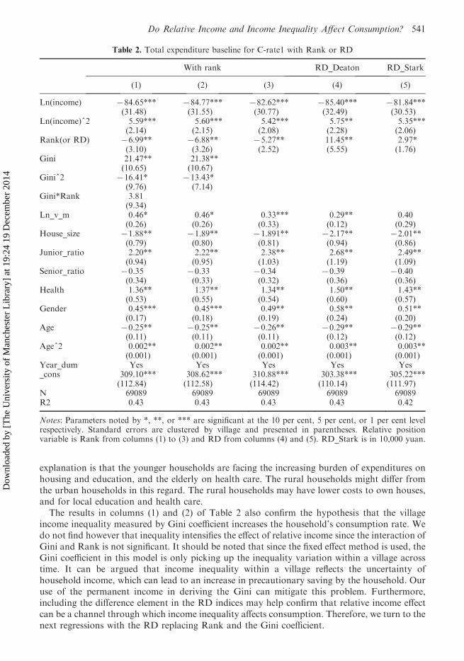
explanation is that the younger households are facing the increasing burden of expenditures onhousing and education, and the elderly on health care. The rural households might differ fromthe urban households in this regard. The rural households may have lower costs to own houses,and for local education and health care.

The results in columns (1) and (2) of Table 2 also confirm the hypothesis that the villageincome inequality measured by Gini coefficient increases the household’s consumption rate. Wedo not find however that inequality intensifies the effect of relative income since the interaction ofGini and Rank is not significant. It should be noted that since the fixed effect method is used, theGini coefficient in this model is only picking up the inequality variation within a village acrosstime. It can be argued that income inequality within a village reflects the uncertainty ofhousehold income, which can lead to an increase in precautionary saving by the household. Ouruse of the permanent income in deriving the Gini can mitigate this problem. Furthermore,including the difference element in the RD indices may help confirm that relative income effectcan be a channel through which income inequality affects consumption. Therefore, we turn to thenext regressions with the RD replacing Rank and the Gini coefficient.

Table 2. Total expenditure baseline for C-rate1 with Rank or RD

With rank RD_Deaton RD_Stark

(1) (2) (3) (4) (5)

Ln(income) 784.65***(31.48)

784.77***(31.55)

782.62***(30.77)

785.40***(32.49)

781.84***(30.53)

Ln(income)^2 5.59***(2.14)

5.60***(2.15)

5.42***(2.08)

5.75**(2.28)

5.35***(2.06)

Rank(or RD) 76.99**(3.10)

76.88**(3.26)

75.27**(2.52)

11.45**(5.55)

2.97*(1.76)

Gini 21.47**(10.65)

21.38**(10.67)

Gini^2 716.41*(9.76)

713.43*(7.14)

Gini*Rank 3.81(9.34)

Ln_v_m 0.46*(0.26)

0.46*(0.26)

0.33***(0.33)

0.29**(0.12)

0.40(0.29)

House_size 71.88**(0.79)

71.89**(0.80)

71.891**(0.81)

72.17**(0.94)

72.01**(0.86)

Junior_ratio 2.20**(0.94)

2.22**(0.95)

2.38**(1.03)

2.68**(1.19)

2.49**(1.09)

Senior_ratio 70.35(0.34)

70.33(0.33)

70.34(0.32)

70.39(0.36)

70.40(0.36)

Health 1.36**(0.53)

1.37**(0.55)

1.34**(0.54)

1.50**(0.60)

1.43**(0.57)

Gender 0.45***(0.17)

0.45***(0.18)

0.49**(0.19)

0.58**(0.24)

0.51**(0.20)

Age 70.25**(0.11)

70.25**(0.11)

70.26**(0.11)

70.29**(0.12)

70.29**(0.12)

Age^2 0.002**(0.001)

0.002**(0.001)

0.002**(0.001)

0.003**(0.001)

0.003**(0.001)

Year_dum Yes Yes Yes Yes Yes_cons 309.10***

(112.84)308.62***(112.58)

310.88***(114.42)

303.38***(110.14)

305.22***(111.97)

N 69089 69089 69089 69089 69089R2 0.43 0.43 0.43 0.43 0.42

Notes: Parameters noted by *, **, or *** are significant at the 10 per cent, 5 per cent, or 1 per cent levelrespectively. Standard errors are clustered by village and presented in parentheses. Relative positionvariable is Rank from columns (1) to (3) and RD from columns (4) and (5). RD_Stark is in 10,000 yuan.

Do Relative Income and Income Inequality Affect Consumption? 541

Dow

nloa

ded

by [

The

Uni

vers

ity o

f M

anch

este

r L

ibra

ry]

at 1

9:24

19

Dec

embe

r 20

14

The last two columns in Table 2 replace the Rank variable with the RD variable, either RDDeaton or RD Stark. Since the RD indices contain both the elements of relative income and themagnitude of differences between households, we no longer include Gini. The results indicatethat relative deprivation significantly increases consumption propensity. The predicted sign forthe RD variable should be opposite to the ones for the standardised rank variable. The resultsconfirm that people are concerned not only about their relative income rank, but also about howfar their income levels are different from those above them. Therefore, the degree of inequalitybetween households can affect consumption through relative comparisons.To investigate the robustness of the regression results for the total expenditure in Table 2, we

report in Table 3 three different alternatives for regressions both with standard income rank andwith Stark’s RD. We are still using the same control variables and only report the parameterestimates for the main variables. For the regression with the rank variable, we use thespecification of column (2) in Table 2. With the RD variable, we use the controls in column (5) ofTable 2. The first alternative is to use C_rate2 as the dependent variable, which has theexpenditures for housing and durable goods smoothed over the years. The second alternative isto use C-rate3 as the dependent variable, which is the sum of the six expenditure categories listedin Table 1. The third alternative is to include the first lag of the dependent variable in theregression, which cuts the sample size and retains only the balanced panel of the households in allfour years of the sample.The results with Rank are reported in the first three rows of Table 3, and those with RD are

reported in the last three rows. The impacts of relative position remain significant for bothmeasures of relative position except for the third row when the lag of consumption is includedwith the Rank variable. With the Rank measurement, using the smoothed consumption rate C-rate2 as the dependent variable seems to produce the best goodness fit as seen from the R2 values.We also note that when the lag of consumption is controlled for, it is not significantly positive.These results suggest the robustness of the relative income effect.

Table 3. Robustness checks for total expenditure, selected coefficients only

Rank/RD(‘0000 yuan) Gini Ln(Income) Lag R2 N

C_rate2(with Rank)

77.15**(3.42)

21.16**(10.57)

783.56***(31.14)

0.44 69089

C_rate3(with Rank)

71.30*(0.79)

4.03*(2.45)

714.05**(7.25)

0.22 69128

C_rate1 w/ laga

(with Rank)71.34***(0.32)

12.75***(2.49)

714.63***b

(2.79)71.19c

(2.19)

728.80***(3.97)

0.0006(0.0007)

779.24d 25990

C_rate2(with RD_Stark)

3.37*(1.9)

780.78***(30.17)

0.43 69089

C_rate3(with RD_Stark)

0.46***(0.08)

713.44**(6.5)

0.22 69128

C_rate1 w/ laga (with RD_Stark) 6.90**(2.81)

728.10***(3.80)

0.0006(0.0007)

755.42d 25990

Notes: Parameters noted by *, **, or *** are significant at the 10 per cent, 5 per cent, or 1 per cent levelrespectively. Robust standard errors are clustered by village and presented in parentheses except for thedynamic model for which the regular standard errors are reported. The control variables are the same asthose in column (2) of Table 2 with Rank or the same as those in column (5) of Table 2 with RD.aThe lagged model is estimated using the Difference-GMM method in Arellano and Bond (1991).bThe coefficient for Gini^2.cThe coefficient for Rank*Gini.dThese numbers are Wald Chi2 statistics.

542 W. Sun & X. Wang

Dow

nloa

ded

by [

The

Uni

vers

ity o

f M

anch

este

r L

ibra

ry]

at 1

9:24

19

Dec

embe

r 20

14

Consumption Expenditure by Categories

We next analyse the impact of relative position on consumption by expenditure categories. Thiswill help to identify whether some types of consumption are considered more positional thanothers. We report here only the results using Stark’s RD variable for the measurement of relativeposition.

The results for the six categories of expenditures are reported in Table 4. We use the samecontrol variables in column (5) of Table 2, but we only list the parameters for the mainvariables. The RD variable has a significant positive impact on expenditure rates for housing,clothing, education, and eating out, negative impact on travel, but is not significant fordurable goods. While it seems hard to distinguish positional from non-positional goods, somehave argued that leisure is a non-positional good (for example, Solnick and Hemenway,1998). This seems to be consistent with the significant negative effect in our regressions of theRD variable on expenditure for travel. The strong positional effect for education is in linewith the argument that people are also concerned with future status since education canbe viewed as an investment for the future. We note that the impact of permanent income onthe consumption rates for most of the categories is negative, but it is not significant fortravel.

We also investigated the robustness of the results for the expenditure categories. Weperformed diagnostic checks on the residuals of different expenditure equations. Most ofthem have strong correlations. Although this does not affect the consistency of the fixedeffects estimation, we also used the Seemingly Unrelated Regression (SUR) method toestimate the consumption category functions. The results for the SUR are very similar toTable 4. The significance levels of the RD indices are the same, so we omit the table hereto save space.2

Analysis by Groups

This section investigates how the above analyses hold for different age groups. This can helpunderstand how people at different life stages care about relative comparison and cancomplement life-cycle theory in explaining age differences in consumption. We consider thedifferences between three age groups, which are reported in the first three rows of Table 5. We

Table 4. Consumption expenditure by categories (with RD)

RD(‘0000 yuan) Ln(Income) R2 N

Housing 0.14***(0.05)

74.61***(0.08)

0.08 69128

Education 0.041***(0.01)

71.39***(0.02)

0.09 69128

Clothing 0.18***(0.02)

74.36***(0.03)

0.40 69128

Eating_out 0.11***(0.02)

72.66***(0.03)

0.14 69128

Durable 0.02(0.01)

70.44***(0.02)

0.01 69128

Travel 70.0038**(0.0017)

0.0018(0.0027)

0.0013 69128

Notes: Parameters noted by *, **, or *** are significant at the 10 per cent, 5 per cent, or 1 per cent levelrespectively. Robust standard errors are clustered by village and presented in parentheses. The controlvariables are the same as those in column (5) of Table 2.

Do Relative Income and Income Inequality Affect Consumption? 543

Dow

nloa

ded

by [

The

Uni

vers

ity o

f M

anch

este

r L

ibra

ry]

at 1

9:24

19

Dec

embe

r 20

14

use the income rank variable here for the measurement of relative position, because income rankoffers more straightforward comparisons in parameter differences. Since it is indicated that C-rate2 produced the best fit, we use this variable as the dependent variable. The results indicatethat all groups are negatively affected by Rank. However, the youngest group, those under theage of 35, are least affected by relative income rank compared with the other two age groups,those between 35 and 55, and those over 55. The youngest households are mostly affected byabsolute income level while income inequality affects only those older than 35. Jin et al. (2011)found that inequality affects the younger group’s consumption more negatively. The differencescould also be due to the difference between our rural data and their urban data. It could also bebecause their model specification did not include the relative income position, which could havecaused estimation bias of other variables in their analysis. These results help us to understand theconsumption and saving behaviour of different age groups in China.

VI. Conclusion

This article has provided strong empirical evidence that household consumption expendituresare strongly affected by the relative income position within a village community aftercontrolling for the absolute income level. Using two measures of relative position, theconsumption rate is negatively related to income rank and positively related to relativedeprivation. The negative impact on total consumption is mainly demonstrated with theexpenditures on housing, education, clothing, and eating out, and weakly demonstrated withdurable goods. We also find that living in a village with higher income inequality willincrease the household’s consumption rate. These findings have important implications formacroeconomic analysis and policy analysis. Since we have found a positive relationshipbetween consumption rate and local inequality, the existing concerns that China’s highincome inequality is driving the low consumption rate are worth further examination. It isstill possible that income inequality has caused other problems in the larger economy thathave affected consumption propensity, and which are not captured in the village relativeincome study. Our study has focused on the consumption propensity of the individualhouseholds. Further research should examine how the aggregate consumption levels in thecommunities and in the whole economy are affected by the households’ desire for socialstatus and the role of income inequality in this matter.

Acknowledgements

This study is supported by the Fundamental Research Funds for the Central Universities, andthe Research Funds of Renmin University of China (10XNJ046). It is also supported by theNational Natural Science Foundation of China under Project 71173228.

Table 5. Analysis by age groups (with Rank)

Dependent variable: Smoothed C_rate 2 Rank Ln(Income) Gini R2 N

Age 535 70.02(0.36)

727.72***(8.00)

71.12(0.92)

0.69 5057

Age 35–55 70.48***(0.09)

732.74***(9.37)

2.51**(0.28)

0.60 39745

Age455 713.24**(5.85)

7108.37***(40.21)

29.77**(14.05)

0.50 24287

Notes: Parameters noted by *, **, or *** are significant at the 10 per cent, 5 per cent, or 1 per cent levelrespectively. Robust standard errors are clustered by village and presented in parentheses. The controlvariables follow column (2) of Table 2.

544 W. Sun & X. Wang

Dow

nloa

ded

by [

The

Uni

vers

ity o

f M

anch

este

r L

ibra

ry]

at 1

9:24

19

Dec

embe

r 20

14

Notes

1. We removed some of the outliers amounting to less than 300 observations in the sample. The first group of removed

observations includes those households that had recorded annual expenditures less than 100 Yuan, most likely as a

result of recording errors. The second group is households that had a negative consumption rate. The third group is

those households that had a consumption rate larger than 1000 per cent. Note that it is possible for the consumption

rate to be larger than 100 per cent because consumption in one year may exceed the total income in that year. We

removed the households with extreme values of consumption rate because they are likely to have been strongly affected

by transitory income. Our initial regression results before removing the outliers did not differ much from the current

results.

2. All additional results are available on request.

References

Abdel-Ghany, M., Silver, J.L. and Gehlken, A. (2002) Do consumption expenditures depend on the household’s relative

position in the income distribution? International Journal of Consumer Studies, 1 (1), 2–6.

Alpizar, F., Carlsson, F. and Johansson-Stenman, O. (2005) How much do we care about absolute versus relative income

and consumption? Journal of Economic Behavior and Organization, 56 (3), 405–421.

Arellano, M. and Bond, S. R. (1991) Some tests of specification for panel data: Monte Carlo evidence and an application

to employment equations. Review of Economic Studies, 58, pp. 277–297.

Benjamin, D., Brandt L. and Giles, J. (2011) Did higher inequality impede growth in rural China? The Economic Journal,

121 (557), 1281–1309.

Brady, D.S. and Friedman, R.D. (1947) Savings and the income distribution, in: Studies in Income and Wealth (Vol. 10)

(New York: National Bureau of Economic Research), 247–265.

Brown, P.H., Bulte, E. and Zhang, X. (2011) Positional spending and status seeking in rural China. Journal of

Development Economics, 96(1), 139–149.

Chamon, M. and Prasad, E. (2010) Why are saving rates of urban households in China rising? American Economic

Journal (Macroeconomics), 2(1), 93–130.

Clark, A.E. and Oswald, A.J. (1996) Satisfaction and comparison income. Journal of Public Economics, 61 (3), 359–381.

Clark, A.E., Frijters, P. and Shields, M.A. (2008) Relative income, happiness and utility: an explanation for the Easterlin

paradox and other puzzles. Journal of Economic Literature, 46 (1), 95–144.

Corneo, G. and Olivier, J. (2001) Status, the distribution of wealth, and growth. Scandinavian Journal of Economics,

103(2), 283–293.

Deaton, A. (2001) Relative deprivation, inequality, and mortality. NBER Working Paper, No8099, Cambridge, MA:

National Bureau of Economics Research.

Duesenberry, J. S. (1949) Income, Saving and the Theory of Consumer Behavior (Cambridge, MA: Harvard University

Press)..

Dupor, B. and Liu, W.F. (2003) Jealousy and equilibrium overconsumption. American Economic Review, 93(1), 423–428.

Easterlin, R. (1974) Does economic growth improve the human lot? Some Empirical Evidence, in: Nations and Households

in Economic Growth: Essays in Honor of Moses Abramovitz (New York: Academic Press).

Easterlin, R.A. (1995) Will raising the incomes of all increase the happiness of all? Journal of Economic Behavior and

Organization, 27 (1), 35–47.

Frank, R. H. (1985) Choosing the Right Pond. Oxford: Oxford University Press.

Frank, R. H. (1999) Luxury fever. New York: Free Press.

Frank, R. (1997) The frame of reference as a public good. The Economic Journal, 107 (445),. 1832–1847.

Frank, R. (2005) Are concerns about relative income relevant for public policy? American Economic Association Papers

and Proceedings, 95 (2), 137–141.

Frank, R. H., Ostvik-White, B. and Levine, A. (2005) Expenditure cascades. Cornell University, Department of

Economics (Mimeo).

Friedman, M. (1956) A Theory of the Consumption Function (Princeton, NJ: Princeton University Press).

Giles, J. (2006) Is life more risky in the open? Household risk-coping and the opening of China’s labour markets. Journal

of Development Economics, 81 (1), 25–60.

Harbaugh, R. (1996) Falling behind the Joneses: relative consumption and the growth-savings paradox. Economics

Letters, 53 (3), 297–304.

Harbaugh, R. (2004) China’s High Savings Rates, Chinese conference volume: The Rise of China Revisited: Perception

and Reality (Taipei). Available at: http://www.bus.indiana.edu/riharbau/harbaugh-chuxu.pdf

Jin, Ye, Li, H. and Wu, B. (2011) Income Inequality, Consumption, and Social-Status Seeking. Journal of Comparative

Economics, 39(2), 191–204.

Keynes, J.M. (1936) The General Theory of Employment, Interest, and Money (London: Macmillan).

Knight, J. Song, L. and Gunatilaka, R. (2009) Subjective well-being and its determinants in rural China, China Economic

Review, 20 (4), 635–649.

Do Relative Income and Income Inequality Affect Consumption? 545

Dow

nloa

ded

by [

The

Uni

vers

ity o

f M

anch

este

r L

ibra

ry]

at 1

9:24

19

Dec

embe

r 20

14

Knight, J. and Gunatilaka, R. (2010) The rural-urban divide in China: income but not happiness? Journal of Development

Studies, 46, (3), 506–534.

Kosicki, G. (1987) A test of the relative income hypothesis. Southern Economic Journal, 54 (2), 422–434.

Kuijs, L. (2005) Investment and Saving in China, in: World Bank Policy Research Working Paper Series 3633, June.

(Washington, DC).

Ling, D. C. (2009) Do the Chinese ‘Keep up with the Jones’? Implications of peer effects, growing economic disparities

and relative deprivation on health outcomes among older adults in China. China Economic Review, 20 (1), 65–81.

Luttmer, E.F.P. (2005) Neighbors as negatives: relative earnings and well-being. The Quarterly Journal of Economics, 120

(3), 963–1002.

McBride, M. (2001) Relative-income effects on subjective well-being in the cross-section. Journal of Economic Behavior

and Organization, 45 (3), 251–278.

Modigliani, F. (1970) The life cycle hypothesis of saving and intercountry differences in the saving ratio, in: W.A. Eltis,

M.F.G. Scott, and J.N. Wolfe (eds) Induction, Growth and Trade (Oxford: Clarendon Press), 197–225.

Modigliani, F. and Shi Larry Cao (2004) The Chinese saving puzzle and the life-cycle hypothesis. Journal of Economic

Literature, 42 (1), 145–170.

Palley, T.I. (2010) The relative permanent income theory of consumption: A synthetic Keynes–Duesenberry–Friedman

model. Review of Political Economy, 22 (1), 41–56.

Pollak, R.A. (1976) Interdependent preferences. American Economic Review, 66 (3), 309–20.

Solnick, S. and Hemenway, D. (1998) Is more always better? A survey on positional goods. Journal of Economic Behavior

and Organization, 37 (3), 373–383.

Stark, O. (2006) Status aspirations, wealth inequality, and economic growth. Review of Development Economics, 10 (1),

171–176.

Stark, O. and Taylor, J. E. (1991) Migration incentives, migration types: the role of relative deprivation. Economic

Journal, 101 (408), 1163–1178.

Stark, O. and Yitzhaki, S. (1988) Labor migration as a response to relative deprivation. Journal of Population Economics,

1 (1), 57–70.

Toche, Patrick. (2003) Keeping up with the Joneses and income risk: revisiting the growth-saving paradox. Working

Paper, City University of Hong Kong, Department of Economics and Finance.

Veblen, T. (1899, 1949) The Theory of the Leisure Class (New York: Macmillan).

Wildman, J. (2003) Income related inequalities in mental health in Great Britain: Analyzing the causes of health

inequality over time. Journal of Health Economics, 22 (2), 295–312.

546 W. Sun & X. Wang

Dow

nloa

ded

by [

The

Uni

vers

ity o

f M

anch

este

r L

ibra

ry]

at 1

9:24

19

Dec

embe

r 20

14