Science of the Total Environment 574 (2017) 191–203

Contents lists available at ScienceDirect

Science of the Total Environment

j ourna l homepage: www.e lsev ie r .com/ locate /sc i totenv

Review

Do drivers of biodiversity change differ in importance across marineand terrestrial systems — Or is it just different researchcommunities' perspectives?

Sonja Knapp a,⁎, Oliver Schweiger a, Alexandra Kraberg b, Harald Asmus c, Ragnhild Asmus c, Thomas Brey d,e,Stephan Frickenhaus f,g, Julian Gutt h, Ingolf Kühn a, Matthias Liess i, Martin Musche a, Hans-O. Pörtner j,Ralf Seppelt k, Stefan Klotz a, Gesche Krause l

a UFZ - Helmholtz-Centre for Environmental Research, Department Community Ecology, Theodor-Lieser-Str. 4, 06120 Halle (Saale), Germanyb Alfred Wegener Institute, Helmholtz Centre for Polar and Marine Research, Division Biosciences/Shelf Sea System Ecology, Kurpromenade 201, Helgoland, Germanyc Alfred Wegener Institute, Helmholtz Centre for Polar and Marine Research, Wadden Sea Station Sylt, 25992 List, Germanyd Alfred Wegener Institute, Helmholtz Centre for Polar and Marine Research, Division Biosciences/Functional Ecology, Am Handelshafen 12, 27570 Bremerhaven, Germanye University Bremen, Germanyf Alfred Wegener Institute, Helmholtz Centre for Polar and Marine Research, Division Biosciences/Scientific Computing, Am Handelshafen 12, 27570 Bremerhaven, Germanyg University of Applied Sciences Bremerhaven, An der Karlstadt 8, 27568 Bremerhaven, Germanyh Alfred Wegener Institute, Helmholtz Centre for Polar and Marine Research, Division Biosciences/Bentho-Pelagic Processes, Am Alten Hafen 26, 27568 Bremerhaven, Germanyi UFZ - Helmholtz-Centre for Environmental Research, Department System-Ecotoxicology, Permoserstr. 15, 04318 Leipzig, Germanyj Alfred Wegener Institute, Helmholtz Centre for Polar and Marine Research, Division Biosciences/Integrative Ecophysiology, Am Handelshafen 12, 27570 Bremerhaven, Germanyk UFZ - Helmholtz-Centre for Environmental Research, Department Computational Landscape Ecology, Permoserstr. 15, 04318 Leipzig, Germanyl Alfred Wegener Institute, Helmholtz Centre for Polar and Marine Research, Division Climate Sciences/Climate Dynamics, Bussestr. 24, 27570 Bremerhaven, Germany

H I G H L I G H T S G R A P H I C A L A B S T R A C T

• Global change affects biodiversityacross the marine and terrestrial realm.

• We rate global change impacts by usingexpert questionnaires and literature re-view.

• Marine and terrestrial scientists largelydiffer in their judgement of impacts.

• Literature shows that terrestrial andmarine ecosystems follow similar prin-ciples.

• Impacts on marine and terrestrial biodi-versity will converge increasingly.

⁎ Corresponding author.E-mail addresses: sonja.knapp@ufz.de (S. Knapp), oliv

Ragnhild.Asmus@awi.de (R. Asmus), Thomas.Brey@awi.dmatthias.liess@ufz.de (M. Liess), martin.musche@ufz.de (Gesche.Krause@awi.de (G. Krause).

http://dx.doi.org/10.1016/j.scitotenv.2016.09.0020048-9697/© 2016 The Authors. Published by Elsevier B.V

a b s t r a c t

a r t i c l e i n f o

Article history:Received 17 June 2016Received in revised form 26 August 2016Accepted 1 September 2016Available online xxxx

Editor: J Jay Gan

Cross-system studies on the response of different ecosystems to global changewill support our understanding ofecological changes. Synoptic views on the planet's twomain realms, themarine and terrestrial, however, are rare,owing to the development of rather disparate research communities. We combined questionnaires and a litera-ture review to investigate how the importance of anthropogenic drivers of biodiversity change differs amongma-rine and terrestrial systems and whether differences perceived bymarine vs. terrestrial researchers are reflectedby the scientific literature. This included asking marine and terrestrial researchers to rate the relevance of

er.schweiger@ufz.de (O. Schweiger), Alexandra.Kraberg@awi.de (A. Kraberg), Harald.Asmus@awi.de (H. Asmus),e (T. Brey), Stephan.Frickenhaus@awi.de (S. Frickenhaus), Julian.Gutt@awi.de (J. Gutt), ingolf.kuehn@ufz.de (I. Kühn),M. Musche), Hans.Poertner@awi.de (H.-O. Pörtner), ralf.seppelt@ufz.de (R. Seppelt), stefan.klotz@ufz.de (S. Klotz),

. This is an open access article under the CC BY-NC-ND license (http://creativecommons.org/licenses/by-nc-nd/4.0/).

192 S. Knapp et al. / Science of the Total Environment 574 (2017) 191–203

Table 1The history of the use of land and sea differs (numbers indthe terrestrial realm.

Land/sea use Terres

Hunting/fishing(referring to Homo sapiens)

200.00

Food sampling(referring to Homo sapiens)

200.00

Agriculture 11.000

Aquaculture/mariculture(i.e. marine aquaculture)

Up to

Share of total areaagriculture/mariculture

38% of

Organisms used as human food resources Primaconsu

Domestication of plants and animals 11.000

different drivers of global change for either marine or terrestrial biodiversity. Land use and the associated loss ofnatural habitats were rated asmost important in the terrestrial realm,while the exploitation of the sea by fishingwas rated asmost important in the marine realm. The relevance of chemicals, climate change and the increasingatmospheric concentration of CO2 were rated differently for marine and terrestrial biodiversity respectively. Yet,our literature review provided less evidence for such differences leading to the conclusion that while the historyof the use of land and sea differs, impacts of global change are likely to become increasingly similar.

© 2016 The Authors. Published by Elsevier B.V. This is an open access article under the CC BY-NC-ND license(http://creativecommons.org/licenses/by-nc-nd/4.0/).

Keywords:Biological invasionsCarbon dioxideChemical pollutantsClimate changeDelphi-assessmentNutrient inputs

Contents

1. Introduction . . . . . . . . . . . . . . . . . . . . . . . . . . . . . . . . . . . . . . . . . . . . . . . . . . . . . . . . . . . . . . 1922. Material and methods . . . . . . . . . . . . . . . . . . . . . . . . . . . . . . . . . . . . . . . . . . . . . . . . . . . . . . . . . . 1933. Results: the Delphi-assessment . . . . . . . . . . . . . . . . . . . . . . . . . . . . . . . . . . . . . . . . . . . . . . . . . . . . . . 1944. Discussion: drivers of biodiversity change in terrestrial and marine ecosystems – differences and similarities. . . . . . . . . . . . . . . . . . . 194

4.1. Does the importance of harvesting (hunting and fishing) differ for marine versus terrestrial biodiversity? . . . . . . . . . . . . . . . . . 1944.2. Does the importance of habitat loss, degradation and fragmentation differ for marine versus terrestrial biodiversity? . . . . . . . . . . . . 1954.3. Does the importance of nutrients differ for marine versus terrestrial biodiversity? . . . . . . . . . . . . . . . . . . . . . . . . . . . 1964.4. Does the importance of chemical pollutants differ for marine versus terrestrial biodiversity? . . . . . . . . . . . . . . . . . . . . . . . 1974.5. Does the importance of climate change (increasing temperatures) differ for marine versus terrestrial biodiversity?. . . . . . . . . . . . . 1984.6. Does the importance of elevated CO2 differ for marine versus terrestrial biodiversity? . . . . . . . . . . . . . . . . . . . . . . . . . . 1994.7. Does the importance of biological invasions differ for marine versus terrestrial biodiversity? . . . . . . . . . . . . . . . . . . . . . . . 200

5. Conclusions. . . . . . . . . . . . . . . . . . . . . . . . . . . . . . . . . . . . . . . . . . . . . . . . . . . . . . . . . . . . . . . 200Acknowledgements . . . . . . . . . . . . . . . . . . . . . . . . . . . . . . . . . . . . . . . . . . . . . . . . . . . . . . . . . . . . . 201Appendix A. Appendix . . . . . . . . . . . . . . . . . . . . . . . . . . . . . . . . . . . . . . . . . . . . . . . . . . . . . . . . . . . 201References. . . . . . . . . . . . . . . . . . . . . . . . . . . . . . . . . . . . . . . . . . . . . . . . . . . . . . . . . . . . . . . . . . 201

1. Introduction

Global change affects ecosystems across the world from the deepseas (Hoegh-Guldberg and Bruno, 2010) to the high mountains (Pauliet al., 2012). Human existence crucially depends on the goods and ser-vices that both marine and terrestrial ecosystems provide (MillenniumEcosystem Assessment, 2005). However, for a sustainable provision ofgoods and services it is crucial to understand how global change affectsdifferent ecosystems, their biodiversity and associated ecosystemfunctions.

Webb (2012) stated that if ecosystems are defined in accordancewith a specific research question, initially perceived differences be-tween these systems can disappear. An example is the comparison ofthe community structure of coral reefs in the marine realm and tropicalforests in the terrestrial realm. In contrast toWebb (2012), Sunday et al.(2012) suggested that even if ecological processes are similar in terres-trial andmarine ecosystems, effects of global change can differ consider-ably between the two. Key questions are why such differences exist andhow ecosystems respond to these differences.

icate the time period for which a cert

trial biome

0 years

0 years

to 12.000 years

10.000 years

land cover

ry producers (crop plants) andmers (mainly herbivores)years

The historic development and current state of biomass extraction –the oldest human impact on ecosystems (Table 1) – differs considerablybetween the terrestrial andmarine realms and somight the response ofbiodiversity to biomass extraction. On land, a 12,000 year-old history ofplant cultivation led to the dominance of artificial production systems atthe level of primary producers. 34% of the earth's ice-free land surfacehas been converted to cropland (12%) and pastures (22%; Ramankuttyet al., 2008). A considerable proportion of forests is not in a pristinestate but heavily transformed by forestry (Food and Agriculture Organi-zation of the United Nations, FAO, 2015). Fishing, collecting and cultiva-tion ofmarine organisms started in an early stage of human existence aswell, similar to hunting and gathering on land (Barrett et al., 2004).While the rate of increase in area used as cropland considerably decel-erated within the last 50 years, the increase in the amount of marineaquaculture seems to stabilize (Fig. 1). According to FAO (2014), marineaquaculture had an average annual growth rate of 6.1% between 2002and 2012. In contrast to terrestrial agricultural production, marineaquaculture is focussed on higher trophic levels such as finfish or crus-taceans, albeit farmed marine plants account for approximately 18% of

ain practice has already been in use). Many kinds of use started later in the marine than in

Marine biome References

200.000 years Anton and Swisher (2004), EncyclopaediaBritannica (2016), Trinkaus (2005)

200.000 years Anton and Swisher (2004), EncyclopaediaBritannica (2016), Trinkaus (2005)Builth et al. (2008), EncyclopaediaBritannica (2016)

ca. 500 years Roberts (2007)

Marginal part of the marine biome FAO; Statistics Division (2015)

Mainly consumers (fish, shellfish)and predators

FAO (2014), FAO; Statistics Division (2015)

ca. 100 years Duarte et al. (2007)

Fig. 1. Decennial increase of the area globally used as cropland (left panel; the y-axisshows the factor by which cropland area increased from one decade to the next basedon one value per decade (black dots)) and annual increase of fish farmed, i.e.aquaculture (right panel; the y-axis shows the factor by which the production (in termsof biomass) of fish farmed increased from one year to the next based on one value peryear (black dots)). The horizontal line indicates y = 1.0 (equal to no change).Data taken from Seppelt et al. (2014) based on Costanza et al. (2007) for cropland andBrown (2012) for fish (here, data earlier than 1950 were not available).

193S. Knapp et al. / Science of the Total Environment 574 (2017) 191–203

total yield already (FAO, 2014). Despite the importance of aquaculture,humans still predominantly act as “hunters and gatherers” ofmarine or-ganisms –much longer than thiswas the case in the terrestrial realm (in2012, N60% of fish resource originated from caught fish; FAO, 2014). Itseems likely that marine biomass extraction will shift frommainly fish-ing to mainly cultivation. Marine catches peaked in 1996 (at 130 Miotonnes) and declined at a mean annual rate of −1.22 Mio tonnes eversince (Pauly and Zeller, 2016).

The extraction of other goods provided by ecosystems has reached apeak, too (such as peat or wood; Seppelt et al., 2014). Moreover, bio-mass extraction is by far not the only anthropogenic driver of biodiver-sity change. Various kinds of land use, nutrient inputs, chemicalpollution, increasing mean and extreme temperatures, elevated CO2

and biological invasions all affect biodiversity (Sala et al., 2000).The ecology of terrestrial and marine ecosystems has been studied

for over a hundred years and human utilization of both realms hasbeen documented going back hundreds or even thousands of years.Nevertheless, mainstream ecology is dominated by terrestrial research(Raffaelli et al., 2005), joint studies are rare (Rotjan and Idjadi, 2013)and different research communities have developed (Stergiou andBrowman, 2005). Marine and terrestrial ecologists even tend to ignoreeach other's work, with especially terrestrial ecologists hardly citingmarine research (Menge et al., 2009). Marine and terrestrial ecosystemshowever, are not disconnected but they are linked with each other, andsome functional principles may be similar. A disconnection of marineand terrestrial research can therefore hamper our understanding ofthe response of biodiversity to global change and consequently our ef-forts to protect and manage ecosystems and their biodiversity(Ruttenberg and Granek, 2011).

By combining review and expert consultation, we asked whetherdrivers of biodiversity change differ in importance across marine andterrestrial systems– orwhether differences are just perceived as a resultof the separation among themarine and terrestrial research community.

2. Material and methods

Going beyond conventional review procedures, we expanded a litera-ture review by means of focus group discussions of both marine and ter-restrial experts as well as a Delphi-assessment. The Delphi-technique(Dalkey and Helmer, 1963) is an expression of expert knowledge used

to achieve convergence of opinion among experts on a specified question.According to Hsu and Sandford (2007) it can be used to

1. explore individual assumptions or knowledge leading to differentjudgments;

2. seek out information that may generate a consensus within therespondent group;

3. correlate informed judgments on a topic spanning a wide range ofdisciplines;

4. educate the respondent group as to the diverse and interrelatedaspects of a topic.

We tailored this method to our specific case, conducting two roundsof expert questioning: In the first round, we provided a questionnaire toa group of marine (N = 90) and terrestrial (N = 90) senior ecologists(hereafter called “experts”; working at our host institutions). Expertscome from two different research institutes, reflecting different re-search communities but sharing an applied and socially relevant re-search focus. The two institutes are the largest of their kind inGermany; they both cover a range of ecological questions and investi-gate these questions internationally, with research sites across theworld.

Experts were asked to rank the impact of selected anthropogenicdrivers of biodiversity change for marine or terrestrial biodiversity (ter-restrial experts ranked drivers of terrestrial biodiversity change;marineexperts ranked drivers ofmarine biodiversity change). 23% of the terres-trial (N = 21) and 20% of the marine (N = 18) experts completed theDelphi-survey. Response rates thus followed the typical rates of onlinequestionnaires, which on average range from 17.1% to 21.5% (Evansand Mathur, 2005; Sax et al., 2003).

The questionnaire contained the following definitions (Table 2):

• Definition of drivers (based on the Millennium EcosystemAssessment, 2005):

◦ Drivers are only anthropogenic drivers that lead to changes inbiodiversity.

◦ Effects are only direct effects of drivers (for example no indirecteffect of CO2 via temperature).

• Definition of biodiversity:◦ Biodiversity concerns all organisational levels from genes to species

and populations, to communities (including taxonomic, functionaland phylogenetic aspects), to entire ecosystems

• Definition of ecosystems:◦ Terrestrial: all terrestrial systems except freshwater systems and soil

systems◦ Marine: all marine systems including coastal waters, offshore and

deep sea areas

We focussed on the following main drivers (Table 2; adapted andextended from Sala et al., 2000): (i) land use/sea use, (ii) chemical in-puts, (iii) climate change (with a focus on changing temperatures),(iv) increasing atmospheric concentration of CO2, and (v) biological in-vasions. “Land/sea use” and “chemical inputs”were further divided into(ia) habitat loss, (ib) habitat degradation, (ic) habitat fragmentation,(id) hunting and fishing; and (iia) nutrients and (iib) pollutants.We de-fined habitat loss as a change in habitat conditionswhich leads to the re-placement by another habitat (such as deforestation to create cropfields), while we define fragmentation as the breaking apart of habitatindependent of habitat loss, i.e. increasing degree of isolation such asthe separation of a forest into several pieces by road construction(Fahrig, 2003). Habitat degradation is defined here as a decline in habi-tat quality (Table 2).

We asked all experts to give a maximum score of 100 to the driverthey considered most important and to rank all other drivers

Table 2Anthropogenic drivers of biodiversity change (based on Sala et al., 2000) with their definitions and examples. For these drivers, we asked experts to score their impacts on biodiversity in aDelphi-assessment (Dalkey and Helmer, 1963).

Driver Sub-category Definition Example

Biologicalinvasions

– Successful establishment of non-native species that spread vigorouslywithin their non-native range and have the potential to causeecological and/or socioeconomic impacts

Spread of the Harlequin ladybird (Harmonia axyridis Pallas), which is apest in orchard crops in America, Africa and Europe and reduces thebiodiversity of other aphidophages and non-pest insects (DAISIEEuropean Invasive Alien Species Gateway, 2008)

Chemicalinputs

Nutrients Nutrients of artificial origin or natural origin but imported into theenvironment by human activities

Nitrogen

Pollutants Chemical substances that are potentially harmful to theenvironment/toxicants

Pesticides

Climatechange

– “A change in the state of the climate that can be identified […] bychanges in the mean and/or the variability of its properties, and thatpersists for an extended period, typically decades or longer.” – here:directly or indirectly caused by human activities (cf. United NationsFramework Convention on Climate Change)

Rise in global temperature due to anthropogenic CO2-emissions

CO2 – Carbon dioxide and the increase of its concentration in the atmosphere –Landuse/seause

Habitat loss A change in habitat conditions that is so strong that it results in theoriginal habitat being replaced by another habitat

Deforestation to create agricultural production sites

Habitatdegradation

Decline in habitat quality Changes of light availability or O2-concentrations

Habitatfragmentation

Breaking apart of habitat without decreasing the total size of availablehabitat (which would be habitat loss), i.e. increasing degree of isolation

Separation of a forest into several pieces by road construction

Hunting,fishing

Killing animal species as food resource, thereby withdrawingindividuals from the environment

–

194 S. Knapp et al. / Science of the Total Environment 574 (2017) 191–203

accordingly between 0 (no impact) and 100. This was done fordrivers i–v, ia–id and iia–iib separately. Different drivers wereallowed to have the same score. The assessment was carried out forbiodiversity changes up to the present day and the reference periodof the questionnaire was restricted to the last 100 years. Expertswere asked to only consider the effect size on biodiversity (i.e. largeor small), not the direction of change (positive or negative).Moreover, we asked experts to score long-term and large-scaleeffects higher than short-term and small-scale effects. Importantly,for each driver, experts were asked to shortly explain theirjudgement and to provide key references.

In the second round (a crucial part in the Delphi process), expertswho had taken part in the first round were provided with the medianand range of scores from the first round and an aggregated version ofthe arguments for high or low scoring. Based on the anonymised argu-ments, the experts then had the possibility to adjust every singlescore. This aimed at a streamlined expert opinion. The final judgementstogether with explanations and key references were compared to a lit-erature review on the effects of global change on terrestrial andmarinebiodiversity. In summary, our approach combines three key steps:

1) the Delphi assessment;2) asking experts to name key publications for each type of global

change (as part of Delphi);3) a literature review focusing on key drivers and references (identified

by (2) and by ourselves).

Only by combining these three steps were we able to efficientlyidentify the most important effects of global change on biodiversity inboth realms. This extends the classical review approaches that couldnot have identified the current research gaps.

3. Results: the Delphi-assessment

In both rounds of our Delphi-assessment, 21 terrestrial and 18 ma-rine expert judgements were obtained.While the second Delphi assess-ment led to a slight reduction in the variability of the range of expertopinion, no major changes in the ranking of importance occurred(Table S1 in Supplementary information).

For marine systems (Fig. 2), sea use and climate change producedthe highest scores in both rounds. The scoring of the impacts of biolog-ical invasions, chemical inputs and enhanced CO2 changed in variancebut not in median or order.

For terrestrial systems (Fig. 2), land use was rated highest with novariance in either round. Chemical inputs were rated second withhigher median weight than in the first round. Climate change wasgiven the same median weight as in the first round but ranked thirdnow. Biological invasions had a lower median weight than in the firstround but stayed in fourth place. Increasing atmospheric concentrationsof CO2 were ranked least important, as in the first round.

Neither for marine nor terrestrial systems (Fig. 3) did the order ormedian weights of habitat loss, degradation, fragmentation and hunt-ing/fishing change from the first to the second round (Table S1). Simi-larly, the importance of nutrients for changes in biodiversity was ratedhigher than for chemical pollutants in both rounds and for both marineand terrestrial (Fig. 4) systems.

4. Discussion: drivers of biodiversity change in terrestrial andmarine ecosystems – differences and similarities

4.1. Does the importance of harvesting (hunting and fishing) differ formarine versus terrestrial biodiversity?

Keeping in mind that our Delphi-assessment focussed on the last100 years and thus omitted earlier developments such as late Quaterna-ry terrestrial megafauna extinctions linked to hunting (Sandom et al.,2014) experts perceived hunting as least important in terrestrial ecosys-tems. In contrast, fishing was ranked as the most important driver ofmarine biodiversity change. This might be explained by major differ-ences in hunting and fishing.

In many terrestrial regions, hunting is strongly regulated today andrestricted to certain target species, whose populations are regularlymonitored and managed accordingly. An example is the European di-rective on the conservation of wild birds (European Commission,2016). However, it was only adopted in 1979 at a time when huntinghad already decimated species numbers, for example the number ofmi-gratory birds (Mcculloch et al., 1992). However, hunting is far more un-specific in other regions of the world and has led to serious populationdeclines, for instance in large-sized mammals and birds in the tropics(Harrison, 2011). Growing demands for bush meat are discussed asthe greatest threat to wildlife in some regions of the world, such asAfrica (Cawthorn and Hoffman, 2015).

In contrast to hunting, many fishing methods (such as bottomtrawling) are either unspecific with multiple target species or yield sig-nificant amounts of non-target bycatch (Davies et al., 2009). Therefore,

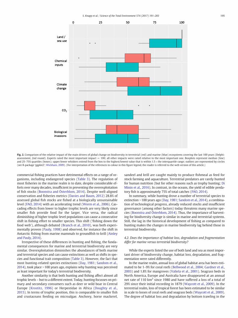
Fig. 2. Comparison of the relative impact of the main drivers of global change on biodiversity in terrestrial (red) and marine (blue) ecosystems covering the last 100 years (Delphi-assessment, 2nd round). Experts rated the most important impact = 100; all other impacts were rated relative to the most important one. Boxplots represent median (line)and 25–75% quartiles (boxes); upper/lower whiskers extend from the box to the highest/lowest value that is within 1.5 ∗ the interquartile range; outliers are represented by circles(see R-package ‘ggplot2’; Wickham, 2009). (For interpretation of the references to colour in this figure legend, the reader is referred to the web version of this article.)

195S. Knapp et al. / Science of the Total Environment 574 (2017) 191–203

commercial fishing practices have detrimental effects on a range of or-ganisms, including endangered species (Table 3). The regulation ofmost fisheries in the marine realm is to date, despite considerable ef-forts overmany decades, insufficient in preventing the overexploitationof fish stocks (Boonstra and Österblom, 2014). Despite well-alignedconservation and fisheries metrics (Davies and Baum, 2012) 28.8% ofassessed global fish stocks are fished at a biologically unsustainablelevel (FAO, 2014) with an accelerating trend (Worm et al., 2006). Cas-cading effects from lower to higher trophic levels are very likely sincesmaller fish provide food for the larger. Vice versa, the radicaldiminishing of higher trophic level populations can cause a consecutiveshift in fishing effort to smaller species. This shift (‘fishing down thefood web’), although debated (Branch et al., 2010), was both experi-mentally proven (Pauly, 1998) and observed, for instance the shift inAntarctic fishing from marine mammals to groundfish to krill (Ainleyand Pauly, 2014).

Irrespective of these differences in hunting and fishing, the funda-mental consequences for marine and terrestrial biodiversity are verysimilar. Overexploitation diminishes the abundances of both marineand terrestrial species and can cause extinctions as well as shifts in spe-cies and functional trait composition (Table 3). However, the fact thatmost hunting-related species extinctions (Day, 1981; Sandom et al.,2014), took place N100 years ago, explains why hunting was perceivedas least important for today's terrestrial biodiversity.

Another similarity is that both hunting and fishing affect almost alltrophic levels – but to a different extent. Today, hunting focusses on pri-mary and secondary consumers such as deer or wild boar in CentralEurope (Krostitz, 1996) or Herpestidae in Africa (Doughty et al.,2015). In terms of trophic position, this is comparable to smaller fishand crustaceans feeding on microalgae. Anchovy, horse mackerel,

sandeel and krill are caught mainly to produce fishmeal as feed forstock farming and aquaculture. Terrestrial predators are rarely huntedfor human nutrition (but for other reasons such as trophy hunting; DiMinin et al., 2016). In contrast, in the oceans, the yield of edible preda-tory fish is approximately 75% of total catches (FAO, 2014).

In summary, while hunting drove a number of terrestrial species toextinction N100 years ago (Day, 1981; Sandom et al., 2014), a combina-tion of technological progress, already reduced stocks and insufficientgovernance (among other factors) today threatens many marine spe-cies (Boonstra and Österblom, 2014). Thus, the importance of harvest-ing for biodiversity change is similar in marine and terrestrial systems.Still, the lag in the historical development of fishing as compared tohunting makes the changes in marine biodiversity lag behind those interrestrial biodiversity.

4.2. Does the importance of habitat loss, degradation and fragmentationdiffer for marine versus terrestrial biodiversity?

While the experts listed the use of both land and sea asmost impor-tant driver of biodiversity change, habitat loss, degradation, and frag-mentation were rated differently.

In the marine realm, annual loss of global habitat area has been esti-mated to be 1–9% for coral reefs (Bellwood et al., 2004; Gardner et al.,2003) and 1.8% for mangroves (Valiela et al., 2001). Seagrass beds inNorth America, Europe and Australia have disappeared at an annualnet rate of 110 km2 since 1980 and have suffered a loss of a total of29% since their initial recording in 1879 (Waycott et al., 2009). In theterrestrial realm, loss of tropical forest has been estimated to be similarin scale to losses of coral reefs and seagrass beds (Waycott et al., 2009).The degree of habitat loss and degradation by bottom trawling in the

Fig. 3. Comparison of the relative impact of subcategories of anthropogenic use of land (red) and sea (blue) on biodiversity covering the last 100 years (Delphi-assessment, 2nd round).Experts rated themost important impact= 100; all other impacts were rated relative to themost important one. Boxplots represent median (line) and 25–75% quartiles (boxes); upper/lower whiskers extend from the box to the highest/lowest value that is within 1.5 ∗ the interquartile range; outliers are represented by circles (see R-package ‘ggplot2’; Wickham, 2009).(For interpretation of the references to colour in this figure legend, the reader is referred to the web version of this article.)

196 S. Knapp et al. / Science of the Total Environment 574 (2017) 191–203

marine realmhave been estimated to be 150-times greater than the ter-restrial area affected by clear-felling of forests (Dulvy et al., 2003). How-ever, while terrestrial habitat loss occurs on large scales, in the marinerealm it is mainly restricted to coastal areas, where sea use has a longtradition (Barrett and Orton, 2016). However intensive utilizationeven in coastal areas started centuries later than in the terrestrialrealm (Duarte et al., 2007), as shown for harvesting. We suggest thatthe differences in scales of observation and in the time period forwhich a certain practice has already been in use (Table 1) add to the dif-ference in perception of habitat loss in marine and terrestrial systems.

Generally, habitat degradation alters the quality and quantity of bio-diversity and their related goods and services. In marine systems,changes in sediment structure, hydrodynamics, and river run-off resultin changes in light availability and O2-concentrations (De'ath andFabricius, 2010; Duarte, 1991) so that species composition can changedramatically, for example from seagrass to macroalgae (McGlathery,2001). Similarly, in terrestrial systems, changes in nutrient supply (es-pecially nitrogen-loads) and related changes in light availability causechanges in species composition (cf. chapter 4.3 “Nutrients”). These sim-ilarities are reflected in the responses of both expert groups in theDelphi-assessment.

The impacts of habitat fragmentation on biodiversity can vary con-siderably among species. While fragmentation such as by roads in-creases isolation among habitat patches, it can also increase edgeeffects. In terrestrial ecosystems, edge effects foster some but disadvan-tage other species, even within one taxon such as different bird guilds(Batary et al., 2014). Similar to roads in the terrestrial realm, pipelines,coastal defences or pylons ofwind turbines form stepping-stones or dis-persal corridors for marine settling larvae. Increasing artificial coastalconstructions, for example are increasingly cited as one reason for theexplosive growth of jellyfish in some geographic areas, which dependon the sessile polyps living on hard substrata (Duarte et al., 2013).

Dispersal potential is basic to the ability of species to copewith isolationin bothmarine and terrestrial systems.While humans have created dis-persal barriers across large parts of the terrestrial world, anthropogenicdispersal barriers in the oceans are mainly restricted to coasts. More-over, dispersal potential has often been assumed to be higher in marinethan terrestrial species (Kinlan and Gaines, 2003). The dispersal poten-tial of sessile and sedentary marine species, for example was estimatedto be 1.5 orders of magnitude higher than for terrestrial plants (Kinlanand Gaines, 2003). However, dispersal is often passive in marine organ-isms in contrast to terrestrial organisms, which are mostly adapted toactive dispersal (Burgess et al., 2016). The fact that extinction rates arepretty similar for marine and non-marine taxa also suggest that marinespecies do not profit from higher dispersal potential (Webb andMindel,2015).

Overall, evidence suggests that the importance of habitat loss, degra-dation and fragmentation is similar in marine and terrestrial systems.The large differences in the experts' perceptions of habitat loss and frag-mentation indicate knowledge gaps, especially for marine species,which are harder to detect and to monitor than terrestrial species.

4.3. Does the importance of nutrients differ for marine versus terrestrialbiodiversity?

Anthropogenic nutrient inputs were regarded as highly important inboth terrestrial and marine ecosystems. This might reflect the fact thatthey have been studied extensively in both realms for over a hundredyears and that their impacts are closely linked to human well-being(Anton et al., 2011).

Nutrients, in particular nitrogen and phosphorus emerge fromvarious anthropogenic sources. In 2010 global anthropogenic nitrogenfixation from fertilizer production, fossil fuel combustion and agricul-tural biogenic fixation even exceeded natural nitrogen fixation

Fig. 4. Comparison of the relative impact of subcategories of chemical inputs on biodiversity in terrestrial (red) and marine (blue) ecosystems covering the last 100 years (Delphi-assessment, 2nd round). Experts rated the most important impact = 100; all other impacts were rated relative to the most important one. Boxplots represent median (line) and25–75% quartiles (boxes); upper/lower whiskers extend from the box to the highest/lowest value that is within 1.5 ∗ the interquartile range; outliers are represented by circles (see R-package ‘ggplot2’; Wickham, 2009). (For interpretation of the references to colour in this figure legend, the reader is referred to the web version of this article.)

197S. Knapp et al. / Science of the Total Environment 574 (2017) 191–203

(210 Tg N yr−1 vs. 203 TgN yr−1; Fowler et al., 2013). Large-scale atmo-spheric deposition of human-induced nutrients affects both terrestrialand marine ecosystems (Meyer et al., 2013; Troost et al., 2013). Addi-tionally, terrestrial ecosystems (especially those used agriculturally)are directly affected through fertilizer application. In the marinerealm, coastal regions and estuaries are affected themost, with nutrientinputs occurring principally via rivers whose nutrient levels have in-creased as a result of land use change and which have been pollutedat least since the mid-19th century (Meybeck and Helmer, 1989). Thisis of course not a universal phenomenon. Efforts to restrict nutrientsin effluents reaching rivers and ultimately the sea mean that manycoastal areas are not seeing eutrophication to the extent that might oth-erwise have occurred. However enclosed, badly mixed areas (possiblyin regionswith a lack of appropriate legislation)might bemore adverse-ly affected.

Although nutrients are essential for plant growth and thus forecosystem functions and services such as human nutrition their ex-cessive input into terrestrial and marine ecosystems has profoundecological consequences. In marine systems, excess nutrients, espe-cially phosphorous and nitrogen boost phytoplankton productionand can shift the whole system from an oligotrophic towards a eutro-phic state, including changes in species composition and food webstructure (Prins et al., 2012; Xie et al., 2015). Microbial decomposi-tion of large algal blooms can cause hypoxic areas with negative con-sequences for all biota and ultimately for human food production. Insummary, effects of eutrophication cascade through marine ecosys-tems from primary producers to top predators and may change spe-cies assemblages at all levels, from macrofauna (Schückel andKröncke, 2013; Snickars et al., 2015) to fish communities (Nixon,1982) and waterbirds (Møller et al., 2015).

In terrestrial ecosystems, enhanced nitrogen supply generally accel-erates plant growth butmay lead to growth reductions, foliar damage ordecreased stress resistance if concentrations exceed species-specific tol-erances (Krupa, 2003). Akin tomarine systems, changes in species com-position towards more nitrogen-tolerant communities represent themost significant impact of excess nutrients and have been reported forplants in grasslands (Dise et al., 2011), arable lands (Meyer et al.,2013), forests (Dirnböck et al., 2014) and urban ecosystems (Knappet al., 2010). This process may go along with a reduction in species rich-ness, particularly in species rich, nutrient-poor habitats (Gerstner et al.,2014; Stevens et al., 2010). Still, it is not necessarily the total amount ofnitrogen but the exceedance of the ecosystem-specific critical load thatresults in changes of community composition and species richness(Dirnböck et al., 2014). Knowledge of the effects of nitrogen on highertrophic levels is limited in terrestrial systems (Dise et al., 2011). Animalsmight be indirectly affected by nitrogen-mediated vegetation changes,habitat structure or food quality as shown by Öckinger et al. (2006)for butterflies – similar to marine food webs.

In summary, although agriculture affects terrestrial ecosystemsmore directly than marine ecosystems, evidence suggests that the ef-fects of human-induced nutrient dynamics (at least for nitrogen andphosphorus) on marine and terrestrial biodiversity are similar.

4.4. Does the importance of chemical pollutants differ formarine versus ter-restrial biodiversity?

The relevance of chemical pollutants for biodiversity change wasgiven a medium score in both realms, with a high variance of assumedimpact.

198 S. Knapp et al. / Science of the Total Environment 574 (2017) 191–203

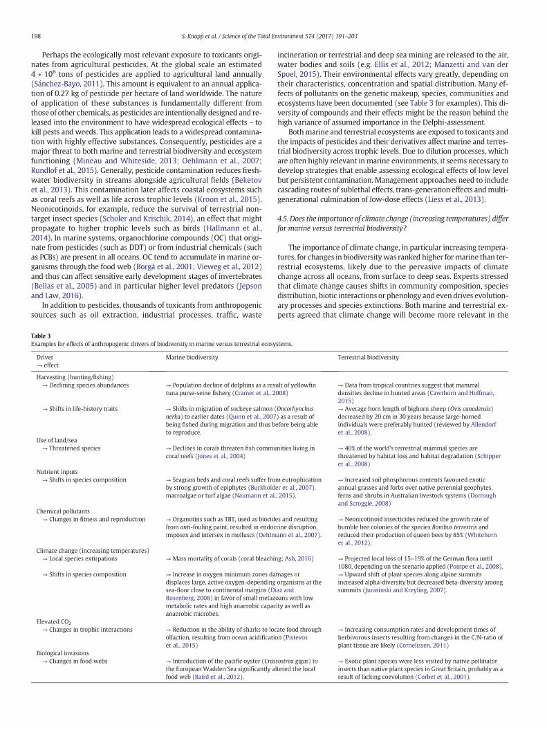
Perhaps the ecologically most relevant exposure to toxicants origi-nates from agricultural pesticides. At the global scale an estimated4 ∗ 106 tons of pesticides are applied to agricultural land annually(Sánchez-Bayo, 2011). This amount is equivalent to an annual applica-tion of 0.27 kg of pesticide per hectare of land worldwide. The natureof application of these substances is fundamentally different fromthose of other chemicals, as pesticides are intentionally designed and re-leased into the environment to have widespread ecological effects – tokill pests and weeds. This application leads to a widespread contamina-tion with highly effective substances. Consequently, pesticides are amajor threat to both marine and terrestrial biodiversity and ecosystemfunctioning (Mineau and Whiteside, 2013; Oehlmann et al., 2007;Rundlof et al., 2015). Generally, pesticide contamination reduces fresh-water biodiversity in streams alongside agricultural fields (Beketovet al., 2013). This contamination later affects coastal ecosystems suchas coral reefs as well as life across trophic levels (Kroon et al., 2015).Neonicotinoids, for example, reduce the survival of terrestrial non-target insect species (Scholer and Krischik, 2014), an effect that mightpropagate to higher trophic levels such as birds (Hallmann et al.,2014). In marine systems, organochlorine compounds (OC) that origi-nate from pesticides (such as DDT) or from industrial chemicals (suchas PCBs) are present in all oceans. OC tend to accumulate in marine or-ganisms through the food web (Borgå et al., 2001; Vieweg et al., 2012)and thus can affect sensitive early development stages of invertebrates(Bellas et al., 2005) and in particular higher level predators (Jepsonand Law, 2016).

In addition to pesticides, thousands of toxicants from anthropogenicsources such as oil extraction, industrial processes, traffic, waste

Table 3Examples for effects of anthropogenic drivers of biodiversity in marine versus terrestrial ecosy

Driver→ effect

Marine biodiversity

Harvesting (hunting/fishing)→ Declining species abundances → Population decline of dolphins as a res

tuna purse-seine fishery (Cramer et al., 2

→ Shifts in life-history traits → Shifts in migration of sockeye salmon (nerka) to earlier dates (Quinn et al., 2007being fished during migration and thus bto reproduce.

Use of land/sea→ Threatened species → Declines in corals threaten fish commu

coral reefs (Jones et al., 2004)

Nutrient inputs→ Shifts in species composition → Seagrass beds and coral reefs suffer fro

by strong growth of epiphytes (Burkholdmacroalgae or turf algae (Naumann et al.

Chemical pollutants→ Changes in fitness and reproduction → Organotins such as TBT, used as biocid

from anti-fouling paint, resulted in endocimposex and intersex in molluscs (Oehlm

Climate change (increasing temperatures)→ Local species extirpations → Mass mortality of corals (coral bleachin

→ Shifts in species composition → Increase in oxygen minimum zones dadisplaces large, active oxygen-dependingsea-floor close to continental margins (DiRosenberg, 2008) in favor of small metazmetabolic rates and high anaerobic capacanaerobic microbes.

Elevated CO2

→ Changes in trophic interactions → Reduction in the ability of sharks to locolfaction, resulting from ocean acidificatioet al., 2015)

Biological invasions→ Changes in food webs → Introduction of the pacific oyster (Cras

the European Wadden Sea significantly afood web (Baird et al., 2012).

incineration or terrestrial and deep sea mining are released to the air,water bodies and soils (e.g. Ellis et al., 2012; Manzetti and van derSpoel, 2015). Their environmental effects vary greatly, depending ontheir characteristics, concentration and spatial distribution. Many ef-fects of pollutants on the genetic makeup, species, communities andecosystems have been documented (see Table 3 for examples). This di-versity of compounds and their effects might be the reason behind thehigh variance of assumed importance in the Delphi-assessment.

Bothmarine and terrestrial ecosystems are exposed to toxicants andthe impacts of pesticides and their derivatives affect marine and terres-trial biodiversity across trophic levels. Due to dilution processes, whichare often highly relevant in marine environments, it seems necessary todevelop strategies that enable assessing ecological effects of low levelbut persistent contamination. Management approaches need to includecascading routes of sublethal effects, trans-generation effects andmulti-generational culmination of low-dose effects (Liess et al., 2013).

4.5. Does the importance of climate change (increasing temperatures) differfor marine versus terrestrial biodiversity?

The importance of climate change, in particular increasing tempera-tures, for changes in biodiversitywas ranked higher formarine than ter-restrial ecosystems, likely due to the pervasive impacts of climatechange across all oceans, from surface to deep seas. Experts stressedthat climate change causes shifts in community composition, speciesdistribution, biotic interactions or phenology and even drives evolution-ary processes and species extinctions. Both marine and terrestrial ex-perts agreed that climate change will become more relevant in the

stems.

Terrestrial biodiversity

ult of yellowfin008)

→ Data from tropical countries suggest that mammaldensities decline in hunted areas (Cawthorn and Hoffman,2015)

Oncorhynchus) as a result ofefore being able

→ Average horn length of bighorn sheep (Ovis canadensis)decreased by 20 cm in 30 years because large-hornedindividuals were preferably hunted (reviewed by Allendorfet al., 2008).

nities living in → 40% of the world's terrestrial mammal species arethreatened by habitat loss and habitat degradation (Schipperet al., 2008)

m eutrophicationer et al., 2007),, 2015).

→ Increased soil phosphorous contents favoured exoticannual grasses and forbs over native perennial geophytes,ferns and shrubs in Australian livestock systems (Dorroughand Scroggie, 2008)

es and resultingrine disruption,ann et al., 2007).

→ Neonicotinoid insecticides reduced the growth rate ofbumble bee colonies of the species Bombus terrestris andreduced their production of queen bees by 85% (Whitehornet al., 2012).

g; Ash, 2016) → Projected local loss of 15–19% of the German flora until1080, depending on the scenario applied (Pompe et al., 2008).

mages ororganisms at theaz andoans with lowity as well as

→ Upward shift of plant species along alpine summitsincreased alpha-diversity but decreased beta-diversity amongsummits (Jurasinski and Kreyling, 2007).

ate food throughn (Pistevos

→ Increasing consumption rates and development times ofherbivorous insects resulting from changes in the C/N-ratio ofplant tissue are likely (Cornelissen, 2011)

sostrea gigas) toltered the local

→ Exotic plant species were less visited by native pollinatorinsects than native plant species in Great Britain, probably as aresult of lacking coevolution (Corbet et al., 2001).

199S. Knapp et al. / Science of the Total Environment 574 (2017) 191–203

future. Terrestrial experts argued that plastic or evolutionary responsesof species might buffer climate change effects.

In the oceans, sea-surface temperature changes between 1901 and2012 reached up to +2.5 K (IPCC, 2014a). The warming rate over landis approximately twice that of the warming rate over the oceans since1979 (IPCC, 2013). The response of organisms to warming is simple:When ambient temperature moves towards and beyond the physiolog-ical limits of a particular organism, individual performance will sufferand the corresponding population will decline once tolerated tempera-ture extremes or the time-limits of tolerance are surpassed (Pörtner,2010; Pörtner and Knust, 2007). Mechanisms that enable organisms tocope with increasing temperatures are the shift of their biogeographicranges and a shift in phenology (see Burrows et al., 2011 and referencestherein).

In the absence of barriers, species may follow the moving isothermsand abandon their original distribution range (Stenseth et al., 2002).The potential for range shifts in the oceans is generally high in relationto the actual climate velocity (Pinsky et al., 2013) and has been estimat-ed between 1.4 and 28 kmper decade (Burrows et al., 2011). This rangeof estimates illustrates that the potential for range shifts depends on theorganism's mobility (Poloczanska et al., 2013) –with a range of marineorganisms not being adapted to active (and thus directed) dispersal(Burgess et al., 2016). Marine dispersal can be further limited by sub-strate availability, light regime, oxygen saturation, pollution, ocean-use or the opportunity to escape poleward (Gutt et al., 2015) – parallelto terrestrial organisms that are restricted to high-altitudemountains orpolar regions (Jurasinski and Kreyling, 2007; Table 3). Range shifts inthe terrestrial realm have been estimated to be 1.5 to 5 times lowerthan in the oceans (Burrows et al., 2011), e.g. 16.9 km/decade polewardacross birds, mammals, arthropods, reptiles and plants (Chen et al.,2011). On the one hand, temperatures are more homogeneous acrossocean than land surfaces – a difference that might explain different ve-locities of marine versus terrestrial organisms (Burrows et al., 2011); onthe other hand, anthropogenic barriers, such as agricultural and built-upareas are mainly terrestrial. However, to which extent such barriersslow down species migration remains largely open (Mendenhall et al.,2012). Generally, the capacity to move depends on the degree ofwarming which in turn defines the velocity of temperature change. Inflat landscapes, for example, the risk is high that most trees, herbs, pri-mates and rodents cannot keep up with the moving isotherms beyond+2 K warming above pre-industrial values (IPCC, 2014b).

Phenological shifts have been observed acrossmarine and terrestrialorganisms (IPCC, 2014a) and are estimated to be 30 to 40% faster in themarine than in the terrestrial realm (Burrows et al., 2011). In both ma-rine and terrestrial systems, both phenological and range shiftsmay alsoalter species interactions (Pörtner et al., 2014). Examples are temporalmismatches (like in the hatching of larvae at a time favorable for theirpredators) and spatial mismatches (such as butterflies and their hostplants shifting their ranges at different pace; Schweiger et al., 2008).

Moreover, in marine systems, the sinking of warmer and saltierwater masses as a result of thermohaline convection alters deep-seaconditions. Atmospheric warming also causes increased stratificationof the upper ocean layer, which in turn expands oxygen minimumzones in the water column (Johnson et al., 2008) and, combined withenhanced eutrophication, leads to changes in species composition(Table 3). Stratification also blocks the flux of nutrients from deeperwater layers to the surface, causing “desertification” of ocean gyres. Asa consequence of a thinner andmore stable surface layer, lower primaryproduction (Sarmiento et al., 2004) and a shift from larger to less di-verse smaller organisms is expected for all oceans. This is the case atleast in the pelagial (Pörtner et al., 2014; Sarmiento et al., 2004; Smithet al., 2008) but polar regions showboth increases (such as in theArctic;Boetius et al., 2013) and decreases in primary productivity, demonstrat-ing that basic biological processes depend on a variety of environmentalfactors (Gutt et al., 2015; Montes-Hugo et al., 2009). In areas ofretreating sea-ice cover, diversity is shifting towards temperate

communities (Wassmann et al., 2011), parallel to the loss of permafrost,which changes terrestrial species richness, abundance and communitycomposition (Rosbakh et al., 2014).

In summary, while temperature changes are faster in the terrestrialrealm, range shifts and phenological shifts are faster in the marinerealm. In addition, the interaction of rising temperatures with thermo-haline convection and ocean stratification lacks an analogy in terrestrialsystems. These differences, togetherwith themanifold effects of climatechange, the time-lag in the response of biodiversity to climate changeand the uncertainties with respect to individual organism's responses(such as dispersal capacity) might explain the uncertainties in experts'judgements and also the higher rating of the importance of climatechange for marine versus terrestrial biodiversity.

4.6. Does the importance of elevated CO2 differ for marine versus terrestrialbiodiversity?

Elevated CO2 was considered to be of least concern in both realmsbut more important in marine than terrestrial systems.

In terrestrial systems, CO2 mainly affects plant growth, water fluxesand trophic interactions. The analysis of satellite observations revealedan increase in foliage cover across global arid zones between 1982 and2010which can be attributed to the increase of atmospheric CO2 duringthat period (Donohue et al., 2013). Free air CO2-enrichment experi-ments showed that elevated CO2 enhances photosynthesis and de-creases transpiration of terrestrial plants with marked differencesamong species and photosynthetic systems (Leakey et al., 2009). More-over, changes in the chemical composition of plant tissues, like increasesin C/N-ratio as a result of increased C-availability, affect higher trophiclevels (Sardans et al., 2012) by decreasing the nutritious value of planttissues (Cornelissen, 2011; Table 3). However, terrestrial animals gener-ally appear less sensitive to the anthropogenic CO2-enrichment in theatmosphere than marine animals due to the inherently higher CO2 par-tial pressures in their body fluids (Ishimatsu et al., 2005).

In marine systems, elevated atmospheric CO2-levels cause an in-creased uptake of CO2 into sea surface waters and thereby ocean acidi-fication. The biological carbon drawdown transfers CO2 from surfaceto deeper waters (Hauck and Völker, 2015). Ocean acidification affectsmarine organisms in multiple ways ranging from metabolic activity ofcalcifiers and non-calcifiers (Liu and He, 2012; Wittmann and Pörtner,2013) to calcification (Kroeker et al., 2013) and habitat shifts as wellas changes in trophic interactions (Table 3) and species abundance(Nagelkerken et al., 2016).Most effects aremediated by CO2 accumulat-ing inside different organisms (Pörtner et al., 2014). Among species en-gineering ecosystems such as warm and cold water corals as well asspecies of commercial interest such as crustaceans, echinoderms andmolluscs CO2 dependent effects reflect differential sensitivities. Impactsare mostly negative and exacerbated by rising ambient CO2 levels(Wittmann and Pörtner, 2013). How these effects will add up at the sys-tem level potentially affecting biodiversity is not yet well understood(Clements and Hunt, 2015).

Another aspect of concern in marine systems is the upward shift ofthe calcium carbonate compensation depth below which aragoniteand calcite dissolve. This impacts especially on existing carbonate struc-tures such as reefs or mounds. By 2100, almost the entire Southern andsubarctic Pacific Oceans are predicted to be undersaturated (Orr et al.,2005). It is further expected that species compositions will shift fromlosers to winners of ocean acidification. Marine biodiversity will de-crease in some important hotspots and foodweb-interactionswill be af-fected. Still, the scale of these impacts is unknown due to insufficientdata. Generally, combined warming and acidification enhance therisks of strong impacts between +1.5 K and +2 K warming abovepre-industrial values as N20 to 50% of corals, echinoderms andmolluscsbecome affected (IPCC, 2014b).

Elevated CO2 is likely to drive changes in the physiological andmorphological traits and in the composition of both marine and

200 S. Knapp et al. / Science of the Total Environment 574 (2017) 191–203

terrestrial species. Present knowledge suggests that extinctions are morelikely in marine systems, which is reflected in our Delphi-assessment.

4.7. Does the importance of biological invasions differ formarine versus ter-restrial biodiversity?

The relevance of biological invasions was rated similar for bothrealms, with medium impacts but large uncertainties. Experts whostressed the relevance of invasions focused on the characteristics of in-vasive species, for example competitive ability. Special focuswas placedhere on the diversity of responses to species invasions from individualsto ecosystem level, such as effects on genetic diversity and trophic inter-actions or the potentially global spread of pathogens. In contrast, ex-perts who stressed that invasions have rather low impacts focused onthe small extent of their impacts, such as invasions beingmost relevanton islands. They argued that there is a lack of evidence of invasions af-fecting ecosystem functioning, implying that invasive species beingrather passengers than drivers of change, pointing towards thecontext-dependency of their impacts.

We conclude from these diverging views that these different percep-tions result from the lack of awidely accepted research definition of “in-vasion” (cf. Table 2 for the definition we adopted), on differences inspatial and temporal study scales, on taxonomic biases (Heger et al.,2013) and on the variety of potential reasons for the success of invasivespecies. For a number of alien species, their success is discussed as a re-sult of the combination of climate change, its effect on relative perfor-mance capacity and fitness (Pörtner et al., 2014) and man as thevector for their invasion.

Despite the apparent lack of an all-encompassing definition of in-vasion, the same mechanisms related to biological invasions arestudied in marine and terrestrial systems such as introduction path-ways. In Europe, 52.2% of alien terrestrial vascular plants were intro-duced as ornamental or horticultural species (Lambdon et al., 2008),while 86% of terrestrial alien arthropods were introduced uninten-tionally (Rabitsch, 2010). For the marine realm, 1369 alien specieshave been identified in Europe. About half of them were introducedunintentionally by shipping, either in ballast water or as hull-fouling organisms (Katsanevakis et al., 2013). Other marine intro-duction pathways are aquaculture, aquarium trade, artificial canalsand scientific in situ experiments.

Where invaders threaten biodiversity, this often results from a com-bination of factors such as the traits of the invader itself and distur-bances in the recipient system. In the Mediterranean, the macroalgaeCaulerpa taxifolia and C. ramosa (accidentally released by aquariummanagers) have displaced large areas of native seagrass meadows(Posidonia oceanica). Healthy seagrass meadows confine Caulerpa tothe periphery of themats, but exposure of Posidonia to high levels of an-thropogenically induced stress (such as wastewater discharges and fishfarm effluents) increases invasibility (Occhipinti-Ambrogi and Savini,2003). A terrestrial example is Splanchnonema platani, a parasite fungusof plane trees originating from the Mediterranean. Heat and droughtpromote its impact on plane in Central Europe, i.e. branch dieback(Kehr and Krauthausen, 2004). Other cconsequences of biological inva-sions for biodiversity in terrestrial systems involve the hybridization ofalien and native species that threatens rare native species (Bleeke et al.,2007) as well as biotic homogenization (Winter et al., 2009). However,extinctions of terrestrial native species by invasive species are mainlyrestricted to islands, where alien vertebrate predators extirpatedmany native birds (Blackburn et al., 2004). As for terrestrial systems,there is poor evidence of biological invasions causing local species ex-tinctions. Nevertheless, marine invaders can considerably impact biodi-versity as competitors or predators of local species or by degradingnative species' habitat (Le Pape et al., 2004). As in terrestrial systems,it is expected that biological invasions - particularly by thermophilicspecies - will lead to biotic homogenization (Occhipinti-Ambrogi andGalil, 2010).

In conclusion, a multitude of biotic introductions have been ob-served in both realms and there does not seem to be much differencein the response of marine versus terrestrial biodiversity to invasions.Despite differences in thedefinition of invasiveness by different authors,it is clear that most introduced species do not become invasive(Richardson and Pyšek, 2006). However, the few that do so can havedevastating ecological effects (Molnar et al., 2008). These contrastscan explain the large uncertainties associatedwith bothmarine and ter-restrial invasions in the Delphi-assessment.

5. Conclusions

We found asymmetries in the experts' perceptions of the impor-tance of different anthropogenic drivers of biodiversity change in ma-rine versus terrestrial systems. Based on the review, we conclude thatthis asymmetry roots in the differences of (i) how and how intenselyhumans use land and sea, (ii) the possibilities to investigate the biodi-versity in marine versus terrestrial ecosystems and (iii) in time-lags ofthe response of biodiversity to global changes. However, differences intime lags as well as in human use are diminishing. On the one hand,the degree and scope of human exploitation of the sea is increasingdrastically (for example with respect to aquaculture; FAO, 2014); onthe other hand, human-induced environmental changes today haveglobal and cross-system impacts rather than “just” regional ones. Weare currently facing a major change in the use of the sea reflecting thehistoric transition from hunters/gatherers to farmers on land. This, to-gether with the other drivers of global change will cause problems formarine ecosystems that will likely be similar to those experienced interrestrial ecosystems already. Still, we have the chance not to repeatmistakes, such as focusing on aquaculture only when most of thehuntable marine organisms have been reduced below levels of com-mercial efficiency or even went extinct. We argue that, even if driversof biodiversity differ in their relative importance for marine versus ter-restrial biodiversity, the protection of marine biodiversity will at leastpartly benefit from the same approaches as does terrestrial biodiversity:

• With respect to harvesting, regulations need to become more effec-tive, especially for marine organisms but also in some terrestrialareas of the world. Additionally, special forms of hunting and fishingshould be used to create benefits for the protection of wildlife. An ex-ample fromNamibia shows that the abundance of wildlife species canincrease when local communities economically benefit from trophyhunting tourism (Di Minin et al., 2016).

• The use of marine areas lags behind land use. Nevertheless, types ofuse that have been restricted to the terrestrial realm are now increas-ingly applied in themarine realm, with aquaculture as the pendant toagriculture being one example and also marine urbanization (con-struction of artificial structures in marine environments) not onlybeing debated but already having ecological consequences (Daffornet al., 2015). The relevance of marine habitat loss should thus not beunderestimated.

• The application of nutrients and chemicals generally needs strongerregulation.While in Europe and the USA there is a will to mitigate eu-trophication, most fertilizers are now produced in Asia and environ-mental problems related to eutrophication are increasingly reportedthere (Li et al., 2015).

• Humanity needs to halt climate change in order to reduce negative ef-fects in both marine and terrestrial systems.

• Similarly, biological invasions are driven by trade and traffic, no mat-ter whether marine or terrestrial (Hulme, 2009). Thus, pathways ofspecies introductions need to be regulated.

From a systems perspective, terrestrial and marine biodiversitychanges follow similar principles. Cross-system synthesis (surveys, insitu experiments and analytical as well as predictive models) is the

201S. Knapp et al. / Science of the Total Environment 574 (2017) 191–203

only way to understand differences and similarities between marineand terrestrial biodiversity change and whether these are driven bythe history of human use or inherent to the respective system.

Acknowledgements

This paper is based on extensive discussions at quarterly workshopmeetings of marine and terrestrial biodiversity researchers from AlfredWegener Institute, Helmholtz Centre for Polar and Marine Research(AWI) and Helmholtz Centre for Environmental Research – UFZ in2014/2015. These workshops were initiated under the umbrella of theGerman Helmholtz Association and its Earth System Knowledge

(i(i(i(i(v

(i(i

(i

(i(i

Platform ESKP (a platform to offer different kind of information inHelmholtz' research field “Earth and Environment”) to intensify the col-laboration among AWI and UFZ. We gratefully thank all experts at AWIand UFZ who participated in the Delphi-assessment and shared theirviews and insights aswell as two anonymous reviewers who gave valu-able comments on a previous version of the article. We acknowledge fi-nancial support by the ESKP initiative. This work is part of the PACES IIResearch Program at AWI, and of the Topic “Land Use, Biodiversity andEcosystemServices” at UFZ. Furthermore, theHelmholtz Office in Berlin,the Climate Service Centre in Hamburg as well as AWI and UFZ are ac-knowledged for hosting our meetings.

Appendix A. Appendix

Table S1

Delphi-assessment of global change drivers of biodiversity. The Delphi technique (Dalkey and Helmer, 1963) is an expression of expert knowledge used to achieve convergence of opinionamong experts on a specified question. The table shows the aggregated results of the Delphi-assessment, 1st and 2nd round, performed by 18 marine and 21 terrestrial senior scienceecologists from Alfred Wegener Institute, Helmholtz Centre for Polar and Marine Research (AWI) and Helmholtz Centre for Environmental Research – UFZ. Originally, 90 marine and90 terrestrial scientists at AWI and UFZwere asked to participate in the assessment.We asked all experts to score the driverwhich they identified asmost important with 100 and to rankall other drivers accordingly between 0 (no impact) and 100. This was done for drivers i–v, ia–id and iia–iib separately.Dalkey N. and Helmer O. (1963). An experimental application of the Delphi method to the use of experts.Management Science, 9, 458–467.

Driver

Median score Minimum score Maximum score

Marine1st

Marine2nd

Terrestrial1st

Terrestrial2nd

Marine1st

Marine2nd

Terrestrial1st

Terrestrial2nd

Marine1st

Marine2nd

Terrestrial1st

Terrestrial2nd

) Land/sea use

92.5 95 100 100 15 15 100 100 100 100 100 100 i) Chemical inputs 40 40 60 65 5 5 5 5 80 80 95 95 ii) Climate Change 75 80 60 60 5 5 10 10 100 100 95 90 v) CO2 40 40 10 10 5 5 3 3 100 100 90 70 ) Biologicalinvasions

50

50 50 40 5 1 2 2 70 70 90 90

a) Habitat loss

40 40 100 100 0 0 40 40 100 100 100 100 b) Habitatdegradation

60

60 80 80 0 0 30 20 100 90 100 100

c) Habitatfragmentation

20

20 60 60 0 0 20 30 100 100 90 80

d) Hunting/fishing

100 100 30 30 0 1 10 10 100 100 85 85 ia) Nutrients 80 80 90 87.5 0 0 5 5 100 100 100 100 ib) Pollutants 70 70 60 50 0 1 10 5 100 100 100 100 (i

References

Ainley, D.G., Pauly, D., 2014. Fishing down the food web of the Antarctic continental shelfand slope. Polar Rec 50, 92–107.

Allendorf, F.W., England, P.R., Luikart, G., Ritchie, P.A., Ryman, N., 2008. Genetic effects ofharvest on wild animal populations. Trends Ecol. Evol. 23, 327–337.

Anton, S.C., Swisher, C.C., 2004. Early dispersals of homo from Africa. Annu. Rev.Anthropol. 33, 271–296.

Anton, A., Cebrian, J., Heck, K.L., Duarte, C.M., Sheehan, K.L., Miller, M.E., et al., 2011.Decoupled effects (positive to negative) of nutrient enrichment on ecosystem ser-vices. Ecol. Appl. 21, 991–1009.

Ash, C., 2016. Bleaching of the Great Barrier Reef. Science 352, 304.Baird, D., Asmus, H., Asmus, R., 2012. Effect of invasive species on the structure and func-

tion of the Sylt-Romo Bight ecosystem, northern Wadden Sea, over three time pe-riods. Mar. Ecol. Prog. Ser. 462, 143–161.

Barrett, J.H., Locker, A.M., Roberts, C.M., 2004. The origins of intensive marine fishing inmedieval Europe: the English evidence. P Roy Soy B-Biol Sci 271, 2417–2421.

Barrett, J.H., Orton, D.C., 2016. Cod and Herring: the archaeology and history of medievalsea fishing. Oxbow Books, Oxford.

Batary, P., Fronczek, S., Normann, C., Scherber, C., Tscharntke, T., 2014. How do edge ef-fects and tree species diversity change bird diversity and avian nest survival inGermany's largest deciduous forest? For. Ecol. Manag. 319, 44–50.

Beketov, M.A., Kefford, B.J., Schafer, R.B., Liess, M., 2013. Pesticides reduce regional biodi-versity of stream invertebrates. PNAS 110, 11039–11043.

Bellas, J., Beiras, R., Marino-Balsa, J., Fernandez, N., 2005. Toxicity of organic compounds tomarine invertebrate embryos and larvae: a comparison between the sea urchin em-bryogenesis bioassay and alternative test species. Ecotoxicology 14, 337–353.

Bellwood, D.R., Hughes, T.P., Folke, C., Nystrom, M., 2004. Confronting the coral reef crisis.Nature 429, 827–833.

Blackburn, T.M., Cassey, P., Duncan, R.P., Evans, K.L., Gaston, K.J., 2004. Avian extinctionand mammalian introductions on oceanic islands. Science 305, 1955–1958.

Bleeke, W., Schmitz, U., Ristow, M., 2007. Interspecific hybridisation between alien andnative plant species in Germany and its consequences for native biodiversity. Biol.Conserv. 137, 248–253.

Boetius, A., Albrecht, S., Bakker, K., Bienhold, C., Felden, J., Fernandez-Mendez, M., et al.,2013. Export of algal biomass from the melting Arctic Sea ice. Science 339,1430–1432.

Boonstra, W.J., Österblom, H., 2014. A chain of fools: or, why it is so hard to stopoverfishing. Marit Stud 13, 1–20.

Borgå, K., Gabrielsen, G.W., Skaare, J.U., 2001. Biomagnification of organochlorines along aBarents Sea food chain. Environ. Pollut. 113, 187–198.

Branch, T.A., Watson, R., Fulton, E.A., Jennings, S., McGilliard, C.R., Pablico, G.T., Ricard, D.,Tracey, S.R., 2010. The trophic fingerprint of marine fisheries. Nature 468, 431–435.

Brown, L.R., 2012. Full Planet, Empty Plates: The New Geopolitics of Food Scarcity. EarthPolicy Institute, Washington, D.C., USAhttp://www.earth-policy.org/books/fpep;.

Builth, H., Kershaw, A.P., White, C., Roach, A., Hartney, L., McKenzie, M., et al., 2008. Envi-ronmental and cultural change on the Mt Eccles lava-flow landscapes of southwestVictoria, Australia. The Holocene 18, 413–424.

Burgess, S.C., Baskett, M.L., Grosberg, R.K., Morgan, S.G., Strathmann, R.R., 2016. When isdispersal for dispersal? Unifying marine and terrestrial perspectives. Biol. Rev. 91,867–882.

Burkholder, J.M., Tomasko, D.A., Touchette, B.W., 2007. Seagrasses and eutrophication.J. Exp. Mar. Biol. Ecol. 350, 46–72.

Burrows, M.T., Schoeman, D.S., Buckley, L.B., Moore, P., Poloczanska, E.S., Brander, K.M., etal., 2011. The pace of shifting climate in marine and terrestrial ecosystems. Science334, 652–655.

Cawthorn, D.M., Hoffman, L.C., 2015. The bushmeat and food security nexus: a global ac-count of the contributions, conundrums and ethical collisions. Food Res. Int. 76,906–925.

Chen, I.C., Hill, J.K., Ohlemüller, R., Roy, D.B., Thomas, C.D., 2011. Rapid range shifts of spe-cies associated with high levels of climate warming. Science 333, 1024–1026.

Clements, J.C., Hunt, H.L., 2015. Marine animal behaviour in a high CO2 ocean. Mar. Ecol.Prog. Ser. 536, 259–279.

Corbet, S.A., Bee, J., Dasmahapatra, K., Gale, S., Gorringe, E., La Ferla, B., et al., 2001. Nativeor exotic? Double or single? Evaluating plants for pollinator-friendly gardens. Ann.Bot. 87, 219–232.

Cornelissen, T., 2011. Climate change and its effects on terrestrial insects and Herbivorypatterns. Neotrop Entomol 40, 155–163.

Costanza, R., Graumlich, L., Steffen, W., Crumley, C., Dearing, J., Hibbard, K., et al., 2007.Sustainability or to collapse: what can we learn from integrating the history ofhumans and the rest of nature? Ambio 36, 522–527.

Cramer, K.L., Perryman, W.L., Gerrodette, T., 2008. Declines in reproductive output in twodolphin populations depleted by the yellowfin tuna purse-seine fishery. Mar. Ecol.Prog. Ser. 369, 273–285.

202 S. Knapp et al. / Science of the Total Environment 574 (2017) 191–203

Dafforn, K.A., Glasby, T.M., Airoldi, L., Rivero, N.K., Mayer-Pinto, M., Johnston, E.L., 2015.Marine urbanization: an ecological framework for designing multifunctional artificialstructures. Front. Ecol. Environ. 13, 82–90.

DAISIE European Invasive Alien Species Gateway. Harmonia Axyridis. July 2014, http://www.europe-aliens.org/speciesFactsheet.do?speciesId=50711; 2008.

Dalkey, N., Helmer, O., 1963. An experimental application of the Delphi method to the useof experts. Manag. Sci. 9, 458–467.

Davies, T.D., Baum, J.K., 2012. Extinction risk and overfishing: reconciling conservationand fisheries perspectives on the status of marine fishes. Sci. Rep. 2, 561.

Davies, R.W.D., Cripps, S.J., Nickson, A., Porter, G., 2009. Defining and estimating globalmarine fisheries bycatch. Mar. Policy http://dx.doi.org/10.1016/j.marpol.2009.01.003.

Day, D., 1981. The Doomsday Book of Animals: A Natural History of Vanished Species. Put-nam: Penguin.

De'ath, G., Fabricius, K., 2010. Water quality as a regional driver of coral biodiversity andmacroalgae on the Great Barrier Reef. Ecol. Appl. 20, 840–850.

Di Minin, E., Leader-Williams, N., Bradshaw, C.J.A., 2016. Banning trophy hunting will ex-acerbate biodiversity loss. Trends Ecol. Evol. 31, 99–102.

Diaz, R.J., Rosenberg, R., 2008. Spreading dead zones and consequences for marine ecosys-tems. Science 321, 926–929.

Dirnböck, T., Grandin, A., Bernhardt-Romermann, M., Beudert, B., Canullo, R., Forsius, M.,et al., 2014. Forest floor vegetation response to nitrogen deposition in Europe. Glob.Chang. Biol. 20, 429–440.

Dise, N.B., Ashmore, M., Belyazid, S., Bleeker, A., Robbink, R., De Vries, W., et al., 2011. Ni-trogen as a threat to European terrestrial biodiversity. In: Sutton, M.A., Howard, C.M.,Erisman, J.W., Billen, G., Bleeker, A., Grennfelt, P., et al. (Eds.), The European NitrogenAssessment. Cambridge University Press, Cambridge, pp. 4463–4494.

Donohue, R.J., Roderick, M.L., McVicar, T.R., Farquhar, G.D., 2013. Impact of CO2 fertiliza-tion on maximum foliage cover across the globe's warm, arid environments.Geophys. Res. Lett. 40, 3031–3035.

Dorrough, J., Scroggie, M.P., 2008. Plant responses to agricultural intensification. J. Appl.Ecol. 45, 1274–1283.

Doughty, H.L., Karpanty, S.M., Wilbur, H.M., 2015. Local hunting of carnivores in forestedAfrica: a meta-analysis. Oryx 49, 88–95.

Duarte, C.M., 1991. Seagrass depth limits. Aquat. Bot. 40, 363–377.Duarte, C.M., Marba, N., Holmer, M., 2007. Rapid domestication of marine species. Science

316, 382–383.Duarte, C.M., Pitt, K.A., Lucas, C.H., Purcell, J.W., Uye, S.-I., Robinson, K., et al., 2013. Is global

ocean sprawl a caus of jellyfish blooms? Front. Ecol. Environ. 11, 91–97.Dulvy, N.K., Sadovy, Y., Reynolds, J.D., 2003. Extinction vulnerability in marine popula-

tions. Fish Fish. 4, 25–64.Ellis, J.I., Fraser, G., Russell, J., 2012. Discharged drilling waste from oil and gas platforms

and its effects on benthic communities. Mar. Ecol. Prog. Ser. 456, 285–302.Encyclopaedia Britannica. Hunting and Gathering Culture. April 2016, https://www.

britannica.com/topic/hunting-and-gathering-culture, 2016.European Commission. The Birds Directive. April 2016, http://ec.europa.eu/environment/

nature/legislation/birdsdirective/index_en.htm, 2016.Evans, J.R., Mathur, A., 2005. The value of online surveys. Internet Res 15, 195–219.Fahrig, L., 2003. Effects of habitat fragmentation on biodiversity. Annu. Rev. Ecol. Syst. 34,

487–515.FAO, 2014. FAO Yearbook. Fishery and Aquaculture Statistics, Rome.FAO, 2015. Global Forest Resources Assessment 2015. Food and Agriculture Organization

of the United Nations, Rome.Fowler, D., Coyle, M., Skiba, U., Sutton, M.A., Cape, J.N., Reis, S., et al., 2013. The global ni-

trogen cycle in the twenty-first century. Philos T R Soc B 368, 1621.Gardner, T.A., Cote, I.M., Gill, J.A., Grant, A., Watkinson, A.R., 2003. Long-term region-wide

declines in Caribbean corals. Science 301, 958–960.Gerstner, K., Dormann, C.F., Stein, A., Manceur, A.M., Seppelt, R., 2014. Effects of land use

on plant diversity — a global meta-analysis. J. Appl. Ecol. 51, 1690–1700.Gutt, J., Bertler, N., Bracegirdle, T.J., Buschmann, A., Comiso, J., Hosie, G., et al., 2015. The

Southern Ocean ecosystem under multiple climate change stresses — an integratedcircumpolar assessment. Glob. Chang. Biol. 21, 1434–1453.

Hallmann, C.A., Foppen, R.P.B., van Turnhout, C.A.M., de Kroon, H., Jongejans, E., 2014. De-clines in insectivorous birds are associated with high neonicotinoid concentrations.Nature 511, 341.

Harrison, R.D., 2011. Emptying the Forest: hunting and the extirpation of wildlife fromtropical nature reserves. Bioscience 61, 919–924.

Hauck, J., Völker, C., 2015. Rising atmospheric CO2 leads to large impact of biology onSouthern Ocean CO2 uptake via changes of the Revelle factor. Geophys. Res. Lett.42, 1459–1464.

Heger, T., Saul, W.C., Trepl, L., 2013. What biological invasions ‘are’ is a matter of perspec-tive. J. Nat. Conserv. 21, 93–96.

Hoegh-Guldberg, O., Bruno, J.F., 2010. The impact of climate change on theworld's marineecosystems. Science 328, 1523–1528.

Hsu, C.-C., Sandford, B.A., 2007. The Delphi technique: making sense of consensus. Practi-cal Assessment, Research & Evaluation 12, 1–8.

Hulme, P.E., 2009. Trade, transport and trouble: managing invasive species pathways inan era of globalization. J. Appl. Ecol. 46, 10–18.

IPCC, 2013. The physical science basis. In: Stocker, T.F., Q, D., Plattner, G.-K., Tignor, M.,Allen, S.K., Boschung, J., et al. (Eds.), Contribution of Working Group I to the Fifth As-sessment Report of the Intergovernmental Panel on Climate Change, p. 1535 (Cam-bridge, United Kingdom and New York, NY, USA).

IPCC, 2014a. Climate Change 2014: Impacts, Adaptation and Vulnerability. Contribution ofWorking group II to the Fifth Assessment Report of the Intergovernmental Panel onClimate Change. http://ipcc-wg2.gov/AR5/;.

IPCC, 2014b. Climate Change 2014: Synthesis Report. Contribution of Working Groups I, IIand III to the Fifth Assessment Report of the Intergovernmental Panel on ClimateChange. IPCC, Geneva, Switzerland.

Ishimatsu, A., Hayashi, M., Lee, K.S., Kikkawa, T., Kita, J., 2005. Physiological effects on fish-es in a high-CO2 world. J Geophys Res-Oceans 110.

Jepson, P.D., Law, R.J., 2016. Marine environment persistent pollutants, persistent threats.Science 352, 1388–1389.

Jones, G.P., McCormick, M.I., Srinivasan, M., Eagle, J.V., 2004. Coral decline threatens fishbiodiversity in marine reserves. PNAS 101, 8251–8253.

Jurasinski, G., Kreyling, J., 2007. Upward shift of alpine plants increases floristic similarityof mountain summits. J. Veg. Sci. 18, 711–718.

Katsanevakis, S., Zenetos, A., Belchior, C., Cardoso, A.C., 2013. Invading Europeanseas: assessing pathways of introduction of marine aliens. Ocean Coast. Manag.76, 64–74.

Kehr, R., Krauthausen, H.J., 2004. First report of damage to plane trees (Platanus ×hispanica) in Germany caused by the fungus Splanchnonema platani. Nachrichtenblattdes Deutschen Pflanzenschutzdienstes 56, 245–251.

Kinlan, B.P., Gaines, S.D., 2003. Propagule dispersal in marine and terrestrial environ-ments: a community perspective. Ecology 84, 2007–2020.

Knapp, S., Kühn, I., Stolle, J., Klotz, S., 2010. Changes in the functional composition of aCentral European urban flora over three centuries. PPEES 12, 235–244.

Kroeker, K.J., Kordas, R.L., Crim, R., Hendriks, I.E., Ramajo, L., Singh, G.S., et al., 2013. Im-pacts of ocean acidification on marine organisms: quantifying sensitivities and inter-action with warming. Glob. Chang. Biol. 19, 1884–1896.

Kroon, F.J., Hook, S.E., Jones, D., Metcalfe, S., Henderson, B., Smith, R., et al., 2015. Alteredtranscription levels of endocrine associated genes in two fisheries species collectedfrom the Great Barrier Reef catchment and lagoon. Mar. Environ. Res. 104, 51–61.

Krostitz, W., 1996. The market for game meat. Fleischwirtschaft 76 (1029-&).Krupa, S.V., 2003. Effects of atmospheric ammonia (NH3) on terrestrial vegetation: a re-

view. Environ. Pollut. 124, 179–221.Lambdon, P.W., Pyšek, P., Basnou, C., Hejda, M., Arianoutsou, M., Essl, F., et al., 2008. Alien

flora of Europe: species diversity, temporal trends, geographical patterns and re-search needs. Preslia 80, 101–149.

Le Pape, O., Guérrault, D., Désaunay, Y., 2004. Effect of invasive mollusc, American slipperlimpet Crepidula fornicata, on habitat suitability for juvenile common sole Solea soleain the Bay of Biscay. Mar. Ecol. Prog. Ser. 277, 107–115.

Leakey, A.D.B., Ainsworth, E.A., Bernacchi, C.J., Rogers, A., Long, S.P., Ort, D.R., 2009. Elevat-ed CO2 effects on plant carbon, nitrogen, and water relations: six important lessonsfrom FACE. J. Exp. Bot. 60, 2859–2876.

Li, Y.Y., Jiao, J.X., Wang, Y., Yang, W., Meng, C., Li, B.Z., et al., 2015. Characteristics of nitro-gen loading and its influencing factors in several typical agricultural watersheds ofsubtropical China. Environ Sci Pollut R 22, 1831–1840.

Liess, M., Foit, K., Becker, A., Hassold, E., Dolciotti, I., Kattwinkel, M., et al., 2013. Culmina-tion of low-dose pesticide effects. Environ. Sci. Technol. 47, 8862–8868.

Liu, W.G., He, M.X., 2012. Effects of ocean acidification on themetabolic rates of three spe-cies of bivalve from southern coast of China. Chin. J. Oceanol. Limnol. 30, 206–211.

Manzetti, S., van der Spoel, D., 2015. Impact of sludge deposition on biodiversity. Ecotox-icology 24, 1799–1814.

Mcculloch, M.N., Tucker, G.M., Baillie, S.R., 1992. The hunting of migratory birds inEurope — a ringing recovery analysis. Ibis 134, 55–65.

McGlathery, K.J., 2001. Macroalgal blooms contribute to the decline of seagrass innutrient-enriched coastal waters. J. Phycol. 37, 453–456.

Mendenhall, C.D., Daily, G.C., Ehrlich, P.R., 2012. Improving estimates of biodiversity loss.Biol. Conserv. 151, 32–34.

Menge, B.A., Chan, F., Dudas, S., Eerkes-Medrano, D., Grorud-Colvert, K., Heiman, K., et al.,2009. Terrestrial ecologists ignore aquatic literature: asymmetry in citation breadthin ecological publications and implications for generality and progress in ecology.J. Exp. Mar. Biol. Ecol. 377, 93–100.

Meybeck, M., Helmer, R., 1989. The quality of rivers— from pristine stage to global pollu-tion. Glob. Planet. Chang. 75, 283–309.

Meyer, S., Wesche, K., Krause, B., Leuschner, C., 2013. Dramatic losses of specialist arableplants in Central Germany since the 1950s/60s-a cross-regional analysis. Divers.Distrib. 19, 1175–1187.

Millennium Ecosystem Assessment, 2005. Ecosystems and HumanWell-being: Synthesis.Island Press, Washington, DC.

Mineau, P., Whiteside, M., 2013. Pesticide acute toxicity is a better correlate of US grass-land bird declines than agricultural intensification. PLoS One 8.

Møller, A.P., Flensted-Jensen, E., Laursen, K., Mardal, W., 2015. Fertilizer leakage to themarine environment, ecosystem effects and population trends of waterbirds inDenmark. Ecosystems 18, 30–44.

Molnar, J.L., Gamboa, R.L., Revenga, C., Spalding, M.D., 2008. Assessing the global threat ofinvasive species to marine biodiversity. Front. Ecol. Environ. http://dx.doi.org/10.1890/070064.

Montes-Hugo, M., Doney, S.C., Ducklow, H.W., Fraser, W., Martinson, D., Stammerjohn,S.E., et al., 2009. Recent changes in phytoplankton communities associated withrapid regional climate change along the western Antarctic peninsula. Science 323,1470–1473.

Nagelkerken, I., Russell, B.D., Gillanders, B.M., Connell, S.D., 2016. Ocean acidificationalters fish populations indirectly through habitat modification. Nat. Clim. Chang.6, 89.

Naumann, M.S., Bednarz, V.N., Ferse, S.C.A., Niggl, W., Wild, C., 2015. Monitoring of coastalcoral reefs near Dahab (Gulf of Aqaba, Red Sea) indicates local eutrophication as po-tential cause for change in benthic communities. Environ. Monit. Assess. 187.

Nixon, S.W., 1982. Nutrient dynamics, primary production and fisheries yields of lagoons.Oceanol. Acta 357-371.

Occhipinti-Ambrogi, A., Galil, B.S., 2010. Alien species as an aspect of global change. AdvLimnol Ocean 1, 199–218.

Occhipinti-Ambrogi, A., Savini, D., 2003. Biological invasions as a component of globalchange in stressed marine ecosystems. Mar. Pollut. Bull. 46, 542–551.

Öckinger, E., Hammarstedt, O., Nilsson, S.G., Smith, H.G., 2006. The relationship betweenlocal extinctions of grassland butterflies and increased soil nitrogen levels. Biol.Conserv. 128, 564–573.

Oehlmann, J., Di Benedetto, P., Tillmann, M., Duft, M., Oetken, M., Schulte-Oehlmann, U.,2007. Endocrine disruption in prosobranch molluscs: evidence and ecological rele-vance. Ecotoxicology 16, 29–43.

Orr, J.C., Fabry, V.J., Aumont, O., Bopp, L., Doney, S.C., Feely, R.A., et al., 2005. Anthropogenicocean acidification over the twenty-first century and its impact on calcifying organ-isms. Nature 437, 681–686.

203S. Knapp et al. / Science of the Total Environment 574 (2017) 191–203

Pauli, H., Gottfried, M., Dullinger, S., Abdaladze, O., Akhalkatsi, M., Alonso, J.L.B., et al.,2012. Recent plant diversity changes on Europe's mountain summits. Science 336,353–355.

Pauly, D., 1998. Fishing down marine food webs. Science 279, 860–863.Pauly, D., Zeller, D., 2016. Catch reconstructions reveal that global marine fisheries catches

are higher than reported and declining. Nat. Commun. 7, 10244.Pinsky, M.L., Worm, B., Fogarty, M.J., Sarmiento, J.L., Levin, S.A., 2013. Marine taxa track

local climate velocities. Science 341, 1239–1242.Pistevos, J.C.A., Nagelkerken, I., Rossi, T., Olmos, M., Connell, S.D., 2015. Ocean acidification

and global warming impair shark hunting behaviour and growth. Sci. Rep. 5.Poloczanska, E.S., Brown, C.J., Sydeman, W.J., Kiessling, W., Schoeman, D.S., Moore, P.J., et

al., 2013. Global imprint of climate change on marine life. Nat. Clim. Chang. 3,919–925.

Pompe, S., Hanspach, J., Badeck, F., Klotz, S., Thuiller, W., Kühn, I., 2008. Climate and landuse change impacts on plant distributions in Germany. Biol. Lett. 4, 564–567.

Pörtner, H.O., 2010. Oxygen- and capacity-limitation of thermal tolerance: a matrix for in-tegrating climate-related stressor effects in marine ecosystems. J. Exp. Biol. 213,881–893.

Pörtner, H.O., Knust, R., 2007. Climate change affects marine fishes through the oxygenlimitation of thermal tolerance. Science 315, 95–97.

Pörtner, H.O., Karl, D.M., Boyd, P.W., Cheung, W.L., Lluch-Cota, S.E., Nojiri, Y., et al., 2014.Ocean systems. In: Field, C.B., Barros, V.R., Dokken, D.J., Mach, K.J., Mastrandrea,M.D., Bilir, T.E., Chatterjee, M., Ebi, K.L., Estrada, Y.O., Genova, R.C., Girma, B., Kissel,E.S., Levy, A.N., MacCracken, S., Mastrandrea, P.R., White, L.L. (Eds.), Climate Change2014: Impacts, Adaptation, and Vulnerability. Part A: Global and Sectoral Aspects.Contribution of Working Group II to the Fifth Assessment Report of the Intergovern-mental Panel on Climate Change. Cambridge University Press, Cambridge, UK andNew York, US, pp. 411–484.

Prins, T.C., Desmit, X., Baretta-Bekker, J.G., 2012. Phytoplankton composition in Dutchcoastal waters responds to changes in riverine nutrient loads. J. Sea Res. 73, 49–62.

Quinn, T.P., Hodgson, S., Flynn, L., Hilborn, R., Rogers, D.E., 2007. Directional selection byfisheries and the timing of sockeye salmon (Oncorhynchus nerka) migrations. Ecol.Appl. 17, 731–739.

Rabitsch, W., 2010. Pathways and vectors of alien arthropods in Europe Chapter 3 In:Roques, A., et al. (Eds.), Alien terrestrial arthropods of Europe 4. BioRisk, pp. 27–34.

Raffaelli, D., Solan, M., Webb, T.J., 2005. Do marine and terrestrial ecologists do it differ-ently? Mar. Ecol. Prog. Ser. 304, 283–289.

Ramankutty, N., Evan, A.T., Monfreda, C., Foley, J.A., 2008. Farming the planet: 1. Geo-graphic distribution of global agricultural lands in the year 2000. Global BiogeochemCy 22.

Richardson, D.M., Pyšek, P., 2006. Plant invasions: merging the concepts of species inva-siveness and community invasibility. Prog. Phys. Geogr. 30, 409–431.

Roberts, C.M., 2007. The Unnatural History of the Sea. Island Press/Shearwater Books,Washington, Covelo, London.

Rosbakh, S., Bernhardt-Römermann, M., Poschlod, P., 2014. Elevationmatters: contrastingeffects of climate change on the vegetation development at different elevations in theBavarian alps. Alp. Bot. 124, 143–154.

Rotjan, R.D., Idjadi, J., 2013. Surf and turf: toward better synthesis by cross-system under-standing. Oikos 122, 285–287.

Rundlof, M., Andersson, G.K.S., Bommarco, R., Fries, I., Hederstrom, V., Herbertsson, L., etal., 2015. Seed coating with a neonicotinoid insecticide negatively affects wild bees.Nature 521, 77–U162.

Ruttenberg, B.I., Granek, E.F., 2011. Bridging the marine–terrestrial disconnect to improvemarine coastal zone science and management. Mar. Ecol. Prog. Ser. 434, 203–212.

Sala, O.E., Chapin III, F.S., Armesto, J.J., Berlow, R., Bloomfield, J., Dirzo, R., et al., 2000. Glob-al biodiversity scenarios for the year 2100. Science 287, 1770–1774.

Sánchez-Bayo F. Impacts of agricultural pesticides on terrestrial ecosystems. In: Sánchez-Bayo F, van den Brink PJ, Mann RM, editors. Ecological Impacts of Toxic Chemicals.Bentham Science, http://ebooks.benthamscience.com/book/9781608051212/, 2011;pp. 63–87.

Sandom, C., Faurby, S., Sandel, B., Svenning, J.C., 2014. Global late Quaternary megafaunaextinctions linked to humans, not climate change. P Roy Soc B-Biol Sci 281.

Sardans, J., Rivas-Ubach, A., Penuelas, J., 2012. The C:N:P stoichiometry of organisms andecosystems in a changing world: a review and perspectives. PPEES 14, 33–47.

Sarmiento, J.L., Slater, R., Barber, R., Bopp, L., Doney, S.C., Hirst, A.C., et al., 2004. Responseof ocean ecosystems to climate warming. Global Biogeochem Cy 18.

Sax, L.J., Gilmartin, S.K., Bryant, A.N., 2003. Assessing response rates and nonresponse biasin web and paper surveys. Res. High. Educ. 44, 409–432.

Schipper, J., Chanson, J.S., Chiozza, F., Cox, N.A., Hoffmann, M., Katariya, V., et al., 2008. Thestatus of the world's land and marine mammals: diversity, threat, and knowledge.Science 322, 225–230.

Scholer, J., Krischik, V., 2014. Chronic exposure of Imidacloprid and Clothianidin reducequeen survival, foraging, and nectar storing in colonies of Bombus impatiens. PLoSOne 9.

Schückel, U., Kröncke, I., 2013. Temporal changes in intertidal macrofauna communitiesover eight decades: a result of eutrophication and climate change. Estuar CoastShelf S 117, 210–218.

Schweiger, O., Settele, J., Kudrna, O., Klotz, S., Kuhn, I., 2008. Climate change can cause spa-tial mismatch of trophically interacting species. Ecology 89, 3472–3479.

Seppelt, R., Manceur, A.M., Liu, J.G., Fenichel, E.P., Klotz, S., 2014. Synchronized peak-rateyears of global resources use. Ecol. Soc. 19.

Smith, C.R., De Leo, F.C., Bernardino, A.F., Sweetman, A.K., Arbizu, P.M., 2008. Abyssal foodlimitation, ecosystem structure and climate change. Trends Ecol. Evol. 23, 518–528.

Snickars, M., Weigel, B., Bonsdorff, E., 2015. Impact of eutrophication and climate changeon fish and zoobenthos in coastal waters of the Baltic Sea. Mar. Biol. 162, 141–151.

Stenseth, N.C., Mysterud, A., Ottersen, G., Hurrell, J.W., Chan, K.S., Lima, M., 2002. Ecolog-ical effects of climate fluctuations. Science 297, 1292–1296.

Stergiou, K.I., Browman, H.I., 2005. Bridging the gap between aquatic and terrestrial ecol-ogy — introduction. Mar. Ecol. Prog. Ser. 304, 271–272.

Stevens, C.J., Thompson, K., Grime, J.P., Long, C.J., Gowing, D.J.G., 2010. Contribution ofacidification and eutrophication to declines in species richness of calcifuge grasslandsalong a gradient of atmospheric nitrogen deposition. Funct. Ecol. 24, 478–484.

Stramma, L., Johnson, G.C., Sprintall, J., Mohrholz, V., 2008. Expanding oxygen-minimumzones in the tropical oceans. Science 320, 655–658.

Sunday, J.M., Bates, A.E., Dulvy, N.K., 2012. Thermal tolerance and the global redistributionof animals. Nat. Clim. Chang. 2, 686–690.

Trinkaus, E., 2005. Early modern humans. Annu. Rev. Anthropol. 34, 207–230.Troost, T.A., Blaas, M., Los, F.J., 2013. The role of atmospheric deposition in the

eutrophixation of the North Sea: a model analysis. J. Mar. Syst. 125, 101–112.Valiela, I., Bowen, J.L., York, J.K., 2001. Mangrove forests: one of the world's threatened

major tropical environments. Bioscience 51, 807–815.Vieweg, I., Hop, H., Brey, T., Huber, S., Ambrose, W.G., Locke, W.L., et al., 2012. Persistent

organic pollutants in four bivalve species from Svalbard waters. Environ. Pollut.161, 134–142.

Wassmann, P., Duarte, C.M., Agusti, S., Sejr, M.K., 2011. Footprints of climate change in theArctic marine ecosystem. Glob. Chang. Biol. 17, 1235–1249.

Waycott, M., Duarte, C.M., Carruthers, T.J.B., Orth, R.J., Dennison, W.C., Olyarnik, S., et al.,2009. Accelerating loss of seagrasses across the globe threatens coastal ecosystems.PNAS 106, 12377–12381.

Webb, T.J., 2012. Marine and terrestrial ecology: unifying concepts, revealing differences.Trends Ecol. Evol. 27, 535–541.

Webb, T.J., Mindel, B.L., 2015. Global patterns of extinction risk inmarine and non-marinesystems. Curr. Biol. 25, 506–511.

Whitehorn, P.R., O'Connor, S., Wackers, F.L., Goulson, D., 2012. Neonicotinoid pesticide re-duces bumble bee colony growth and queen production. Science 336, 351–352.

Wickham, H., 2009. ggplot2: Elegant Graphics for Data Analysis. Springer, New York.Winter, M., Schweiger, O., Klotz, S., Nentwig, W., Andriopoulos, P., Arianoutsou, M., et al.,

2009. Plant extinctions and introductions lead to phylogenetic and taxonomic ho-mogenization of the European flora. PNAS 106, 21721–21725.

Wittmann, A.C., Pörtner, H.O., 2013. Sensitivities of extant animal taxa to ocean acidifica-tion. Nat. Clim. Chang. 3, 995–1001.

Worm, B., Barbier, E.B., Beaumont, N., Duffy, J.E., Folke, C., Halpern, B.S., et al., 2006. Im-pacts of biodiversity loss on ocean ecosystem services. Science 314, 787–790.

Xie, Y.Y., Tilstone, G.H., Widdicombe, C., Woodward, E.M.S., Harris, C., Barnes, M.K., 2015.Effect of increases in temperature and nutrients on phytoplankton community struc-ture and photosynthesis in the western English Channel. Mar. Ecol. Prog. Ser. 519,61–73.