DI

SC

US

SI

ON

P

AP

ER

S

ER

IE

S

Forschungsinstitut zur Zukunft der ArbeitInstitute for the Study of Labor

Do Better Paid Politicians Perform Better?Disentangling Incentives from Selection

IZA DP No. 4400

September 2009

Stefano GagliarducciTommaso Nannicini

Do Better Paid Politicians Perform Better? Disentangling Incentives from Selection

Stefano Gagliarducci Tor Vergata University

and IZA

Tommaso Nannicini

Bocconi University, IGIER and IZA

Discussion Paper No. 4400 September 2009

IZA

P.O. Box 7240 53072 Bonn

Germany

Phone: +49-228-3894-0 Fax: +49-228-3894-180

E-mail: iza@iza.org

Any opinions expressed here are those of the author(s) and not those of IZA. Research published in this series may include views on policy, but the institute itself takes no institutional policy positions. The Institute for the Study of Labor (IZA) in Bonn is a local and virtual international research center and a place of communication between science, politics and business. IZA is an independent nonprofit organization supported by Deutsche Post Foundation. The center is associated with the University of Bonn and offers a stimulating research environment through its international network, workshops and conferences, data service, project support, research visits and doctoral program. IZA engages in (i) original and internationally competitive research in all fields of labor economics, (ii) development of policy concepts, and (iii) dissemination of research results and concepts to the interested public. IZA Discussion Papers often represent preliminary work and are circulated to encourage discussion. Citation of such a paper should account for its provisional character. A revised version may be available directly from the author.

IZA Discussion Paper No. 4400 September 2009

ABSTRACT

Do Better Paid Politicians Perform Better? Disentangling Incentives from Selection*

The wage paid to politicians affects both the choice of citizens to run for an elective office and the performance of those who are appointed. First, if skilled individuals shy away from politics because of higher opportunities in the private sector, an increase in politicians’ pay may change their mind. Second, if the reelection prospects of incumbents depend on their in-office deeds, a higher wage may foster performance. We use data on all Italian municipal governments from 1993 to 2001 and test these hypotheses in a quasi-experimental framework. In Italy, the wage of the mayor depends on population size and sharply rises at different thresholds. We apply a regression discontinuity design to the only threshold that uniquely identifies a wage increase – 5,000 inhabitants – to control for unobservable town characteristics. Exploiting the existence of a two-term limit, we further disentangle the composition from the incentive component of the effect of the wage on performance. Our results show that a higher wage attracts more educated candidates, and that better paid politicians size down the government machinery by improving internal efficiency. Importantly, most of this performance effect is driven by the selection of competent politicians, rather than by the incentive to be reelected. JEL Classification: M52, D72, J45, H70 Keywords: political selection, efficiency wage, term limit, local finance,

regression discontinuity design Corresponding author: Tommaso Nannicini Department of Economics Bocconi University Via Roentgen 1 20136 Milan Italy E-mail: tommaso.nannicini@unibocconi.it

* We thank Alberto Alesina, Marianne Bertrand, Stéphane Bonhomme, Michael Elsby, Nicola Persico, Steve Pischke, Albert Solé, and seminar participants at Universitat de Barcelona, CEMFI, ESSLE-CEPR 2008, IMT Lucca, IGIER-Bocconi, and SOLE 2009 for their insightful comments. We are also grateful to Fabio Albiani from the Italian Ministry of Internal Affairs for invaluable help with data collection, and to Lucia Spadaccini for excellent research assistance. The usual caveat applies.

1 Introduction

Paying politicians is a debated but elusive topic. Firms set the wage of workers to maximize

their profits; politicians set the wage of bureaucrats to maximize either social welfare or

their own interests. For the same reason, citizens—the principal—should set the optimal

compensation of politicians—the agent—according to some welfare criteria. But this is

rarely the case. The wage of elected officials is decided by politicians themselves. And the

public opinion swings from the complaint against the high salaries of the political elite

to the acknowledgment that “if you pay peanuts you get monkeys” also in politics.1 No

evidence unambiguously supports either claim.

The wage paid to elected officials is an important element—although not the only one—

in shaping both the decision to enter politics and the behavior once in office. According

to the standard efficiency wage theory, a salary increase could both attract more skilled

candidates (citizens with higher opportunity costs) and enhance performance (because of

the higher cost of not being reelected). Various models in political economics contain

similar intuitions while adding more structure on the political side—see, among others,

Besley (2004) and Caselli and Morelli (2004). Alternative models, instead, build on some

peculiarities of the political sector to show that, if high-skilled citizens have a comparative

advantage in entering politics—for instance, because of higher post-congressional returns,

as in Mattozzi and Merlo (2008)—paying politicians more may have a crowding-out effect

and decrease the average quality. At the end of the day, the question of whether politicians’

remuneration affects their selection and performance remains empirical.

In this paper, we use a dataset on the mayors of all Italian municipalities from 1993

to 2001 to evaluate the impact of politicians’ remuneration in a quasi-experimental frame-

work. In Italy, the wage of the mayor increases with the size of the resident population, the

motivation for this rule being that, as for companies’ executives, the amount of work and

responsibility grows with the number of people to be managed. The quasi-experimental

framework arises because the wage does not increase monotonically, but sharply changes

at nine different thresholds. As long as population size cannot be manipulated by the

1Other traditional views emphasize that a better pay might also guarantee a broader representationof all social categories, and reduce the incentives for corruption. We focus here on competence andperformance, because other measures of politicians’ quality, such as honesty, are not available.

1

mayor to sort above these thresholds and be paid more, the institutional setting delivers

a clean exogenous variation in the remuneration of politicians. This is not the case with

other observational setups, which are plagued with sizable selection bias if politicians can

set their own wage, or if environmental characteristics influence both the salary and the

opportunity cost of entering politics.

Politicians’ pay is not the only policy decided by the number of resident inhabitants,

though. The size of the municipal council, the electoral rule, and many other policies

vary according to population brackets. After inquiring the Ministry of Internal Affairs

and comparing different legislative sources as a cross-check, we found out that only three

thresholds uniquely identify a wage increase: 1,000, 5,000, and 50,000 inhabitants. How-

ever, we cannot use the 1,000 threshold because of its late introduction (in 2000) and the

50,000 threshold because of sample size limitations. We hence focus on the 5,000 threshold,

at which there is a sharp 33% increase (28% after 2000) in the mayor’s wage. Although the

local effect identified at this threshold may not be easily generalized to higher population

levels, it should be noted that small cities (below 10,000 inhabitants) account for about

90% of all Italian municipalities. Furthermore, the large executive power of mayors, and

the close monitoring put forth by voters especially in small municipalities, fit well with

Besley’s (2004, p. 210) recommendation that agency models on paying politicians “are

most promising when applied in situations where there are directly elected chief execu-

tives with significant discretionary power.” We therefore apply a Regression Discontinuity

Design (RDD) at the 5,000 threshold to control for unobservable town characteristics and

test whether a higher wage attracts individuals with higher opportunity costs (effect of

the wage on political selection) and improves the performance of elected politicians (effect

of the wage on performance).

As for selection, the empirical results show that the 33% wage increase at 5,000 attracts

more educated candidates: from 0.9 to 1.2 years of schooling more, depending on the

specification, which means an increase in education from 6.4% to 8.6% (with respect to an

average of 14 years of schooling in municipalities between 3,000 and 5,000 inhabitants).

There is also evidence that the wage increase attracts more candidates employed in high-

skilled occupations, such as lawyers, professionals, or entrepreneurs. This translates into

more educated (from 0.9 to 1.6 years of schooling more) and high-skilled elected mayors.

2

As for performance, following the literature on political accountability and political

budget cycles, we first look at policies of direct interest to voters, such as taxes, tariffs,

and expenditures.2 We find that better paid politicians reduce the size of the municipal

government. In particular, they lower taxes and tariffs per capita (by about 13% and

86%, respectively) and reduce the amount of personnel and other current expenditures

(by about 11% and 22%, respectively).

This performance result can have two different interpretations. First, more skilled

politicians are better at making the government machinery more efficient, as they reduce

current—instead of capital—expenditure, characterized by sizable passive waste in Italy

(Bandiera, Prat, and Valletti, 2009). Second, the reduction in government size reflects

differences in preferences, with more educated mayors having weaker preferences for re-

distribution and public services (Alesina and Giuliano, 2009). We shed more light on

these alternative explanations by looking at two efficiency indicators for the management

of the municipal government: the speed of revenues collection (that is, the ratio between

collected and assessed revenues) and the speed of payment (that is, the ratio between paid

and committed outlays). Our results show that better paid mayors effectively increase the

speed of revenues collection by 7%. And this supports the interpretation that they are at

least able to make the bureaucratic organization more efficient.

The effect of the wage on performance might be driven by two distinct components:

better paid politicians may act differently because of their higher skills (composition effect

of the wage on performance) or because of enhanced reelection motives (incentive effect

of the wage on performance).3 To disentangle these two channels, we exploit another

institutional feature of the Italian legislation: the existence of a two-term limit. It is true,

indeed, that also mayors with a binding term limit have a lot of incentives to perform well,

including the desire to run for higher offices or to leave a positive legacy, but all of these

motivations do not depend on the wage. Therefore, mayors just below and just above

the 5,000 threshold have identical incentives when they all face a binding term limit. On

the contrary, when the term limit is not binding, their incentives diverge because of the

2As empirical tests of political agency models using budget variables, see—among others—Besley andCase (1995) and List and Sturm (2006). As empirical studies on political budget cycles, see—amongothers—Akhmedov and Zhuravskaja (2004) and Brender and Drazen (2008).

3To avoid confusion between terms, we refer to “selection effect” as the impact of the wage on selection,and to “composition effect” as the selection component of the impact of the wage on performance.

3

different wage they would obtain if reelected. Following a diff-in-diff strategy, we thus

subtract the difference between the performance of second-term mayors just above and

below the threshold from the difference between the performance of first-term mayors just

above and below the threshold, to retrieve an estimate of the (reelection) incentive effect

of the wage on performance. Our results show that most of the performance effect is

driven by the higher competence of the elected mayors, rather than by the incentive to be

reelected. We take this as evidence of the strength of the composition effect. Alternative

explanations for the lack of a (reelection) incentive effect, including strong ideological

preferences by voters, do not receive support from the data.

The paper proceeds as follows. In Section 2, we set the theoretical background and

review the related literature. In Section 3, we formalize our econometric strategy. In

Section 4, we describe the institutional framework and the data. In Section 5, we present

the estimation results and a number of robustness exercises. We conclude with Section 6.

2 Related literature

2.1 Theoretical background

According to the efficiency wage theory, workers’ productivity is increasing in the real wage

they are paid.4 There are three main explanations for why this relationship should hold:

paying workers more reduces shirking because of the higher cost of being fired (Shapiro

and Stiglitz, 1984); it enhances the quality of applicants (Weiss, 1980); and it improves

motivation and group work norms (Akerlof, 1982). If we apply these insights to the labor

market for politicians, we should conclude that a higher wage is likely to improve the

performance of elected officials due to different reasons. First, a higher wage will attract

more skilled individuals (that is, citizens with better outside opportunities in the private

sector) into politics. Second, it will increase the incumbent’s payoff from being reelected;

and this, in turn, will make elected officials more disciplined (e.g., less inclined to extract

rents). Third, it could improve the morale of politicians.

The efficiency wage theory, of course, does not consider many aspects that are specific

to the political arena, such as party selection, campaigning, non-monetary incentives, and

4See Akerlof and Yellen (1986) or Yellen (1984) for a survey of the efficiency wage literature.

4

voters’ preferences. Various models in political economics, however, contain some intu-

itions and predictions of the efficiency wage theory while providing specific insights on the

political side. Besley (2004) builds an agency model with both unobserved heterogeneity in

the congruence of politicians with voters (adverse selection) and unobserved action when

in office (moral hazard). As reelection is the main incentive mechanism, a higher wage

plays a discipline role, that is, it increases performance by forcing dissonant politicians

to extract lower rents. Moreover, a higher wage also increases the fraction of congruent

politicians, who—unlike the dissonant type—earn no rents from entering politics. Caselli

and Morelli (2004) present an adverse selection model where low-quality citizens (“bad

politicians”) have a comparative advantage in holding office, because their market wages

are lower than those of more competent individuals, or because they extract more rents

than more honest individuals. In this framework, a higher salary raises the average quality

of the (self-selected) pool of politicians. Persson and Tabellini (2000) propose a career-

concern model where forward-looking voters use past performance to estimate the ability

of the incumbent. As a result, also low-ability officials have an incentive to cut rents and

increase the political output in order to be reelected. In this framework, the higher the

wage, the lower politicians’ rents and the higher performance.

The prediction that the quality of politicians is increasing in their wage, however, is

not unanimously shared by the literature. Actually, a number of models suggest that the

opposite may be true in all the circumstances in which high-quality citizens have other

incentives to enter politics, because a higher remuneration has the indirect effect of making

all the other (low-quality) candidates more willing to run.5 For example, Mattozzi and

Merlo (2008) propose a dynamic model where there are both “career politicians,” who stay

in politics until retirement, and individuals with “political careers,” who stay in politics for

a while in order to signal their true ability to the private sector. In this framework, a wage

increase lowers the average quality of citizens who have political careers, because politics

becomes a relatively more attractive option for all levels of skills, and it has an ambiguous

effect on the average quality of career politicians, because also high-ability incumbents

are more willing to remain in politics. Gagliarducci, Nannicini, and Naticchioni (2008)

5Messner and Polborn (2004) come to a similar conclusion, although in their case the rationale is thatcompetent candidates have an higher incentive to free-ride on mediocre candidates, under the assumptionthat the attractiveness of public life is low.

5

study the effect of outside income on political selection: if politicians can keep their

private business while appointed and election boosts the private returns of high-ability

citizens, then outside income can induce equilibria with positive sorting, where a wage

increase would make the public office relatively more attractive for low-ability citizens.

Finally, Besley (2005) introduces another explanation of the negative impact of the wage

on politicians’ quality: if public service motivations are strong, a higher remuneration

lowers the relative attractiveness of politics for public-spirited individuals.

2.2 Empirical studies

Despite this rich set of theoretical predictions, there are only a few empirical studies on the

impact of politicians’ remuneration. Di Tella and Fisman (2004) look at gubernatorial pay

in the US from 1950 to 1990 and find that wages respond to changes in state income and

taxes per capita. In particular, governors obtain a one percent pay cut for each ten percent

increase in per capita taxation, and there is some evidence that this negative tax elasticity

is an implicit form of performance pay. Besley (2004) analyzes the same data on US

gubernatorial pay. He finds that the congruence between the ideological positions of the

governor and citizens—as measured by established surveys—is positively associated with

the governor’s wage. Diermeier, Keane, and Merlo (2005) estimate a structural dynamic

model of congressional careers in the US, finding that congressional experience significantly

increases post-congressional wages in the private sector. Keane and Merlo (2007) use the

same model to evaluate the effect of reducing the relative wage of congressmen. They find

that a wage reduction would induce more skilled politicians to exit Congress (where skills

refer to the ability to win elections), but this is not true for “achievers,” that is, for those

who perform better in terms of legislative and policy goals.

An empirical exercise similar to ours was presented, independently, by Ferraz and

Finan (2009). To the best of our knowledge, this is the only other paper that builds

on a clean exogenous variation in the pay of elected officials. They implement an RDD

exploiting a Brazilian constitutional amendment that introduced caps on the wages of

municipal councillors (vereadores) according to population size. They show that a higher

wage attracts more candidates and, in particular, more educated ones; they also find

that legislative productivity—measured as the number of bills submitted and approved—

6

increases with the salary. Despite the similarity between the two approaches, however,

our paper is distinct in many respects. First, we implement a sharp (instead of a fuzzy)

RDD, because in Italy it is the statutory wage that varies with population size. Second,

we focus on the mayor as the chief executive of the municipality, and then we look at

budget indicators as performance outcomes. Third—and most important—we disentangle

between the composition and the incentive effect of the wage on performance, exploiting

the existence of a two-term limit.

To a lower extent, our paper also relates to other strands of the political economics

literature. Recent studies have implemented RDD exercises based on policies that vary

with population size at the local level, in order to estimate the effect of the number of

legislators on the size of government (Petterson-Lindbom, 2008), the effect of the electoral

rule on economic policy (Bordignon and Tabellini, 2008; Chamon et al., 2008), the effect

of fiscal windfalls on corruption and political selection (Brollo et al., 2009), or the effect

of direct versus representative democracy (Petterson-Lindbom and Tyrefors, 2009). Our

results could also be compared with the studies on the effect of civil servants’ pay on

corruption (Besley and McLaren, 1993; Van Rijckeghem and Weder, 2001), although we

look at elected officials and focus on administrative IQ rather than honesty. Finally, as we

make the assumption that a binding term limit wipes out reelection incentives, we borrow

insights from the vast literature on political accountability and term limits.6

3 Econometric framework

3.1 Identifying the effect of the wage

In this section, we formalize the evaluation framework that allows us to identify the effect

of the wage on both the selection and the in-office performance of politicians. In particular,

we want to test the following hypotheses.

(H1) A higher wage attracts more citizens with high opportunity costs into politics, that

is, more skilled individuals with high alternative remunerations in the private sector

(effect of the wage on political selection).

6See—among others—Rogoff (1990), Besley and Case (1995), Maskin and Tirole (2004), List andSturm (2006), Smart and Sturm (2006), and Ferraz and Finan (2007).

7

(H2) A higher wage enhances the performance of elected officials (effect of the wage on

performance). This may in turn be determined by two channels:

(H2.1) a higher wage attracts more skilled citizens into politics (composition effect);

(H2.2) a higher wage increases the cost of not being reelected (incentive effect).

A major empirical difficulty in identifying the effect of politicians’ remuneration on

their selection and performance is the absence of a truly exogenous variation in the amount

they are paid. It is not hard to imagine rent-seeking politicians raising their own salary,

or righteous representatives giving up part of their remuneration to prove their public-

spiritedness. For the same reason, in the absence of an exogenous rule, one might also

expect the social environment (e.g., the level of economic development, social capital, or

corruption) to determine both politicians’ wage and characteristics. To overcome these

endogeneity problems, we exploit the Italian policy of paying mayors according to the

population size of the municipality.

Define Xi as the characteristics of citizens who run for mayor in town i; Yi as some

performance indicator; Pi as the population size; and Wi as the wage paid to the mayor.

By law, the wage sharply increases at the population threshold Pc. That is, if Pi ≥ Pc,

then Wi = Wh; if Pi < Pc, then Wi = W` < Wh. To formalize the idea that both the

characteristics of politicians and the performance of the mayor depend on the wage, we use

a potential outcome framework. Define Xi(Wk) ≡ Xik, with k ∈ `, h, as the potential

characteristics of politicians in town i if the wage is equal to Wk. Similarly, Yi(Wk) ≡ Yik,

with k ∈ `, h, captures the potential performance of the mayor in town i if the wage is

equal to Wk. In the following, we omit the subscript i, for all variables are town-specific.

For each town, we either observe X` and Y` or Xh and Yh, according to the wage of the

mayor. The estimand of interest is the average treatment effect for the entire population

or for a subpopulation of cities (Ω): E[Xh − X`|i ∈ Ω] and E[Yh − Y`|i ∈ Ω]. The

conditional comparison of X and Y in towns with W = W` against towns with W = Wh

does not generally provide an unbiased estimate of the average treatment effect, because

towns with different unobservable characteristics may endogenously choose the mayor’s

remuneration, as discussed above. The fact that in Italy the salary of mayors depends on

the population size, however, can be exploited to implement a sharp RDD and estimate

8

the causal effect of the wage on both X and Y . In order to do this, we need to make the

following assumptions.7

Assumption 1 E[X`|P = p] and E[Xh|P = p] are continuous in p at Pc.

Assumption 2 E[Y`|P = p] and E[Yh|P = p] are continuous in p at Pc.

In other words, the potential characteristics of the political elite and the potential

performance of the mayor, which may depend on the population size P , should not display

any discontinuity at Pc. Although both assumptions are more than plausible in our setting,

two caveats are in order. First, if mayors can manipulate population size and sort above

the threshold, treatment assignment is no longer exogenous. Second, if there is another

policy that depends on population size and shares the same threshold Pc, the effect of the

wage is confounded with the effect of this other policy and cannot be identified. It is thus

important to check whether the data provide evidence of sorting around the threshold,

and to be sure that other policies do not vary across the same population threshold.

Under Assumption 1, it is straightforward to show that E[X`|P = Pc] = limP↑PcX

and E[Xh|P = Pc] = limP↓PcX. We can thus identify the treatment effect of the wage on

political selection as

τsel ≡ E[Xh − X`|P = Pc] = limP↓Pc

X − limP↑Pc

X. (1)

Similarly, under Assumption 2, the treatment effect of the wage on performance is

τper ≡ E[Yh − Y`|P = Pc] = limP↓Pc

Y − limP↑Pc

Y. (2)

Both τsel and τper are defined as local effects, because they capture the impact of the wage

only for towns around the threshold Pc. As usual in RDD, the gain in internal validity

comes at the price of lower external validity.

3.2 Disentangling incentives from selection

To empirically disentangle (H2.1) and (H2.2) as alternative explanations of the impact of

the wage on performance, we need to introduce further notation and assumptions. Using

7See Hahn, Todd, and Van der Klaauw (2001) for a discussion of identification assumptions in RDD.

9

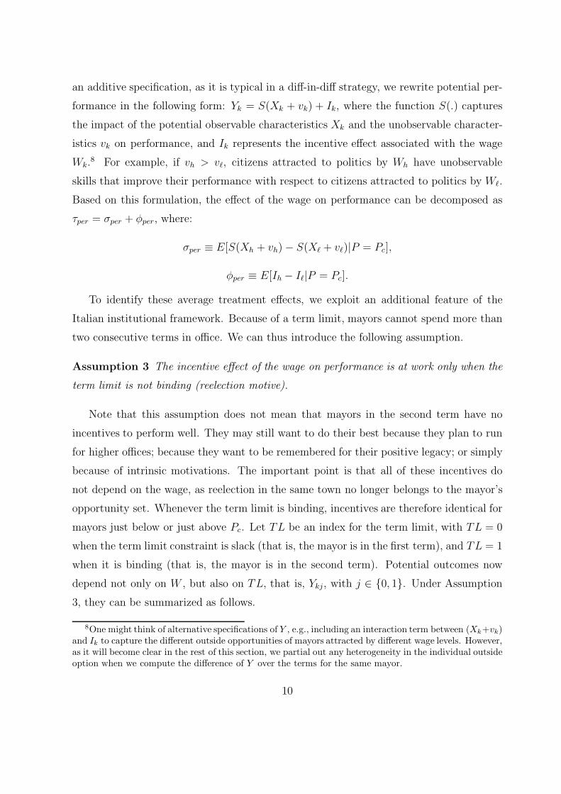
an additive specification, as it is typical in a diff-in-diff strategy, we rewrite potential per-

formance in the following form: Yk = S(Xk + vk) + Ik, where the function S(.) captures

the impact of the potential observable characteristics Xk and the unobservable character-

istics vk on performance, and Ik represents the incentive effect associated with the wage

Wk.8 For example, if vh > v`, citizens attracted to politics by Wh have unobservable

skills that improve their performance with respect to citizens attracted to politics by W`.

Based on this formulation, the effect of the wage on performance can be decomposed as

τper = σper + φper, where:

σper ≡ E[S(Xh + vh) − S(X` + v`)|P = Pc],

φper ≡ E[Ih − I`|P = Pc].

To identify these average treatment effects, we exploit an additional feature of the

Italian institutional framework. Because of a term limit, mayors cannot spend more than

two consecutive terms in office. We can thus introduce the following assumption.

Assumption 3 The incentive effect of the wage on performance is at work only when the

term limit is not binding (reelection motive).

Note that this assumption does not mean that mayors in the second term have no

incentives to perform well. They may still want to do their best because they plan to run

for higher offices; because they want to be remembered for their positive legacy; or simply

because of intrinsic motivations. The important point is that all of these incentives do

not depend on the wage, as reelection in the same town no longer belongs to the mayor’s

opportunity set. Whenever the term limit is binding, incentives are therefore identical for

mayors just below or just above Pc. Let TL be an index for the term limit, with TL = 0

when the term limit constraint is slack (that is, the mayor is in the first term), and TL = 1

when it is binding (that is, the mayor is in the second term). Potential outcomes now

depend not only on W , but also on TL, that is, Ykj, with j ∈ 0, 1. Under Assumption

3, they can be summarized as follows.

8One might think of alternative specifications of Y , e.g., including an interaction term between (Xk+vk)and Ik to capture the different outside opportunities of mayors attracted by different wage levels. However,as it will become clear in the rest of this section, we partial out any heterogeneity in the individual outsideoption when we compute the difference of Y over the terms for the same mayor.

10

W = W` W = Wh

TL=0 Y`0 = S(X`0 + v`0) + I` Yh0 = S(Xh0 + vh0) + Ih

TL=1 Y`1 = S(X`1 + v`1) + exp Yh1 = S(Xh1 + vh1) + exp

Here, exp stands for administrative experience, which we assume to affect performance

independently of the wage schedule.9 The above table shows that mayors in the first

term and mayors in the second term might have different skills. In particular, as long as

performance is relevant for reelection, we expect mayors at TL = 1 to be more skilled

according to both observable and unobservable characteristics. In general: S(Xk0 +vk0) 6=

S(Xk1 + vk1). If we restrict the analysis to the sample of politicians who are elected for

two consecutive terms, however, we have that: S(Xk0 + vk0) = S(Xk1 + vk1).

In this context, we can identify the overall effect of the wage on performance as:

τper = E[Yh0 − Y`0|P = Pc] = limP↓Pc|TL=0

Y − limP↑Pc|TL=0

Y, (3)

where the first equality follows from Assumption 3 and the sample restriction to politicians

elected for two consecutive terms, while the second equality follows from Assumption 2.

Similarly, we can identify the composition effect and the incentive effect of the wage

on performance, respectively, as:

σper = E[Yh1 − Y`1|P = Pc] = limP↓Pc|TL=1

Y − limP↑Pc|TL=1

Y, (4)

φper = E[(Yh0 − Yh1) − (Y`0 − Y`1)|P = Pc] =

=

(

limP↓Pc|TL=0

Y − limP↑Pc|TL=0

Y

)

−

(

limP↓Pc|TL=1

Y − limP↑Pc|TL=1

Y

)

.(5)

In both equations, the first equality follows from Assumption 3 and the sample restriction

to reelected politicians, while the second equality follows from Assumption 2.10

9If experience enhanced performance more for high-skilled than for low-skilled mayors (that is, exph >

exp`), we could still identify the overall effect of the wage on performance, but we would overestimate(underestimate) the composition (incentive) component. In Section 5.3, we come back to this point froman empirical point of view and show that the effect of administrative experience on performance does notdepend on political selection.

10To leave the framework as simple as possible, so far we have not contemplated the pure motivationaleffect of an increase in the salary on performance (Akerlof, 1982). Experimental evidence suggests thiseffect being relatively small (Gneezy and List, 2006). If there were any, the potential performance shouldbe rewritten as: Yk = S(Xk+vk)+Ik +Mk, where Mk represents the morale effect associated with the wageWk. It is easy to show that, while φper would still identify the incentive effect (Mk would cancel out in

11

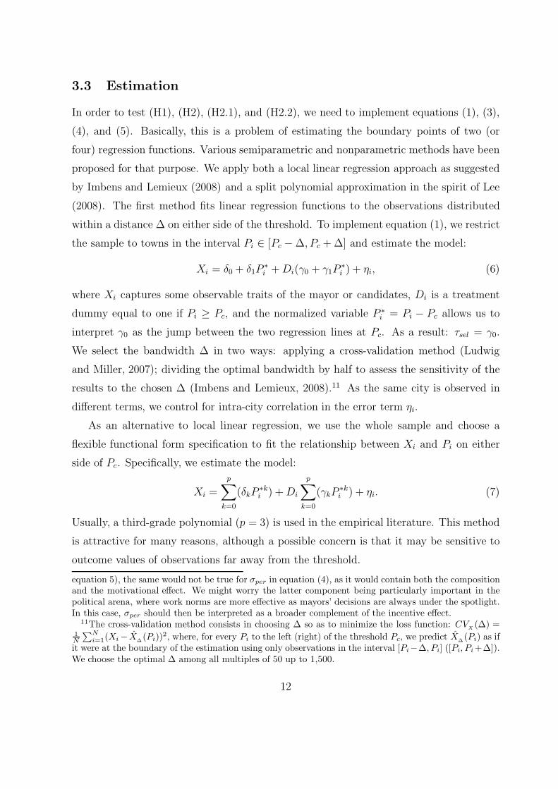
3.3 Estimation

In order to test (H1), (H2), (H2.1), and (H2.2), we need to implement equations (1), (3),

(4), and (5). Basically, this is a problem of estimating the boundary points of two (or

four) regression functions. Various semiparametric and nonparametric methods have been

proposed for that purpose. We apply both a local linear regression approach as suggested

by Imbens and Lemieux (2008) and a split polynomial approximation in the spirit of Lee

(2008). The first method fits linear regression functions to the observations distributed

within a distance ∆ on either side of the threshold. To implement equation (1), we restrict

the sample to towns in the interval Pi ∈ [Pc − ∆, Pc + ∆] and estimate the model:

Xi = δ0 + δ1P∗i + Di(γ0 + γ1P

∗i ) + ηi, (6)

where Xi captures some observable traits of the mayor or candidates, Di is a treatment

dummy equal to one if Pi ≥ Pc, and the normalized variable P ∗i = Pi − Pc allows us to

interpret γ0 as the jump between the two regression lines at Pc. As a result: τsel = γ0.

We select the bandwidth ∆ in two ways: applying a cross-validation method (Ludwig

and Miller, 2007); dividing the optimal bandwidth by half to assess the sensitivity of the

results to the chosen ∆ (Imbens and Lemieux, 2008).11 As the same city is observed in

different terms, we control for intra-city correlation in the error term ηi.

As an alternative to local linear regression, we use the whole sample and choose a

flexible functional form specification to fit the relationship between Xi and Pi on either

side of Pc. Specifically, we estimate the model:

Xi =

p∑

k=0

(δkP∗ki ) + Di

p∑

k=0

(γkP∗ki ) + ηi. (7)

Usually, a third-grade polynomial (p = 3) is used in the empirical literature. This method

is attractive for many reasons, although a possible concern is that it may be sensitive to

outcome values of observations far away from the threshold.

equation 5), the same would not be true for σper in equation (4), as it would contain both the compositionand the motivational effect. We might worry the latter component being particularly important in thepolitical arena, where work norms are more effective as mayors’ decisions are always under the spotlight.In this case, σper should then be interpreted as a broader complement of the incentive effect.

11The cross-validation method consists in choosing ∆ so as to minimize the loss function: CVX

(∆) =1

N

∑N

i=1(Xi − X

∆(Pi))

2, where, for every Pi to the left (right) of the threshold Pc, we predict X∆(Pi) as if

it were at the boundary of the estimation using only observations in the interval [Pi−∆, Pi] ([Pi, Pi +∆]).We choose the optimal ∆ among all multiples of 50 up to 1,500.

12

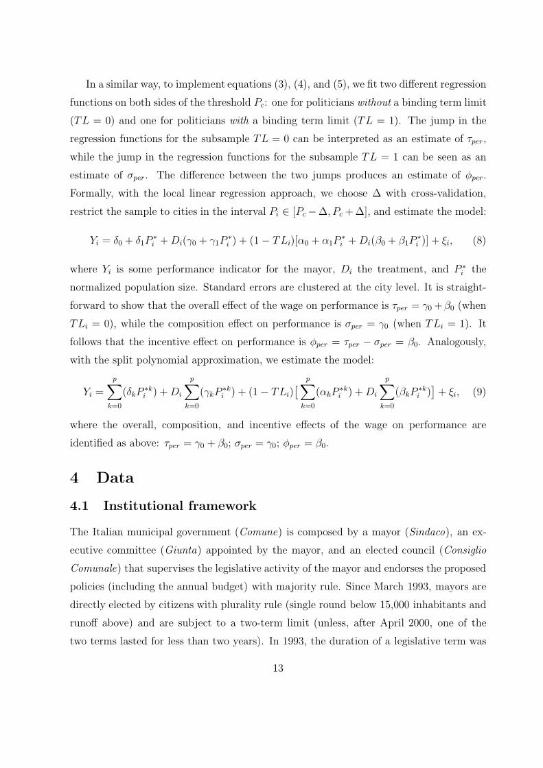
In a similar way, to implement equations (3), (4), and (5), we fit two different regression

functions on both sides of the threshold Pc: one for politicians without a binding term limit

(TL = 0) and one for politicians with a binding term limit (TL = 1). The jump in the

regression functions for the subsample TL = 0 can be interpreted as an estimate of τper ,

while the jump in the regression functions for the subsample TL = 1 can be seen as an

estimate of σper. The difference between the two jumps produces an estimate of φper.

Formally, with the local linear regression approach, we choose ∆ with cross-validation,

restrict the sample to cities in the interval Pi ∈ [Pc −∆, Pc + ∆], and estimate the model:

Yi = δ0 + δ1P∗i + Di(γ0 + γ1P

∗i ) + (1 − TLi)[α0 + α1P

∗i + Di(β0 + β1P

∗i )] + ξi, (8)

where Yi is some performance indicator for the mayor, Di the treatment, and P ∗i the

normalized population size. Standard errors are clustered at the city level. It is straight-

forward to show that the overall effect of the wage on performance is τper = γ0 +β0 (when

TLi = 0), while the composition effect on performance is σper = γ0 (when TLi = 1). It

follows that the incentive effect on performance is φper = τper − σper = β0. Analogously,

with the split polynomial approximation, we estimate the model:

Yi =

p∑

k=0

(δkP∗ki ) + Di

p∑

k=0

(γkP∗ki ) + (1 − TLi)

[

p∑

k=0

(αkP∗ki ) + Di

p∑

k=0

(βkP∗ki )

]

+ ξi, (9)

where the overall, composition, and incentive effects of the wage on performance are

identified as above: τper = γ0 + β0; σper = γ0; φper = β0.

4 Data

4.1 Institutional framework

The Italian municipal government (Comune) is composed by a mayor (Sindaco), an ex-

ecutive committee (Giunta) appointed by the mayor, and an elected council (Consiglio

Comunale) that supervises the legislative activity of the mayor and endorses the proposed

policies (including the annual budget) with majority rule. Since March 1993, mayors are

directly elected by citizens with plurality rule (single round below 15,000 inhabitants and

runoff above) and are subject to a two-term limit (unless, after April 2000, one of the

two terms lasted for less than two years). In 1993, the duration of a legislative term was

13

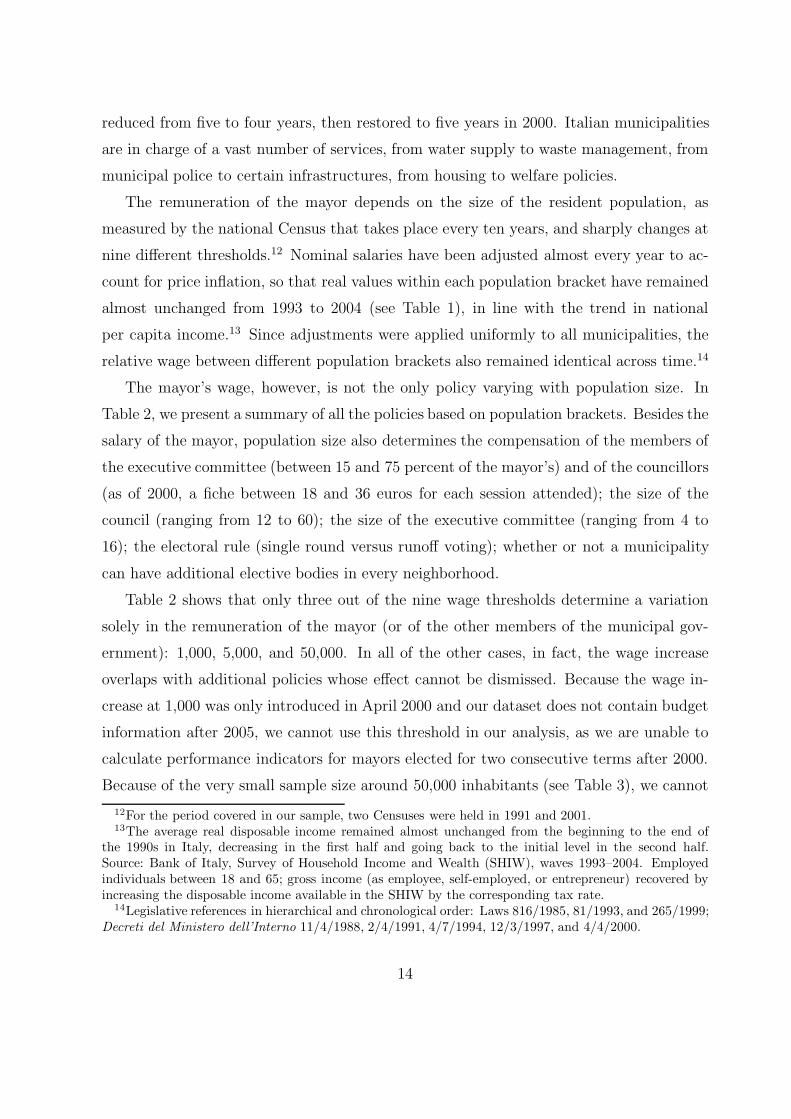
reduced from five to four years, then restored to five years in 2000. Italian municipalities

are in charge of a vast number of services, from water supply to waste management, from

municipal police to certain infrastructures, from housing to welfare policies.

The remuneration of the mayor depends on the size of the resident population, as

measured by the national Census that takes place every ten years, and sharply changes at

nine different thresholds.12 Nominal salaries have been adjusted almost every year to ac-

count for price inflation, so that real values within each population bracket have remained

almost unchanged from 1993 to 2004 (see Table 1), in line with the trend in national

per capita income.13 Since adjustments were applied uniformly to all municipalities, the

relative wage between different population brackets also remained identical across time.14

The mayor’s wage, however, is not the only policy varying with population size. In

Table 2, we present a summary of all the policies based on population brackets. Besides the

salary of the mayor, population size also determines the compensation of the members of

the executive committee (between 15 and 75 percent of the mayor’s) and of the councillors

(as of 2000, a fiche between 18 and 36 euros for each session attended); the size of the

council (ranging from 12 to 60); the size of the executive committee (ranging from 4 to

16); the electoral rule (single round versus runoff voting); whether or not a municipality

can have additional elective bodies in every neighborhood.

Table 2 shows that only three out of the nine wage thresholds determine a variation

solely in the remuneration of the mayor (or of the other members of the municipal gov-

ernment): 1,000, 5,000, and 50,000. In all of the other cases, in fact, the wage increase

overlaps with additional policies whose effect cannot be dismissed. Because the wage in-

crease at 1,000 was only introduced in April 2000 and our dataset does not contain budget

information after 2005, we cannot use this threshold in our analysis, as we are unable to

calculate performance indicators for mayors elected for two consecutive terms after 2000.

Because of the very small sample size around 50,000 inhabitants (see Table 3), we cannot

12For the period covered in our sample, two Censuses were held in 1991 and 2001.13The average real disposable income remained almost unchanged from the beginning to the end of

the 1990s in Italy, decreasing in the first half and going back to the initial level in the second half.Source: Bank of Italy, Survey of Household Income and Wealth (SHIW), waves 1993–2004. Employedindividuals between 18 and 65; gross income (as employee, self-employed, or entrepreneur) recovered byincreasing the disposable income available in the SHIW by the corresponding tax rate.

14Legislative references in hierarchical and chronological order: Laws 816/1985, 81/1993, and 265/1999;Decreti del Ministero dell’Interno 11/4/1988, 2/4/1991, 4/7/1994, 12/3/1997, and 4/4/2000.

14

use this threshold either. As a result, we focus on the 5,000 threshold only, with an addi-

tional caveat: since 2002, municipalities above 5,000 are subject to the Internal Stability

Pact, a set of rules decided by the national government to improve fiscal discipline at the

municipality level. We therefore restrict our analysis to mayoral terms from 1993 to 2001.

As of 2000, the real gross wage of the mayor ranges from 1,291 euros per month for

municipalities with less than 1,000 inhabitants up to 7,798 euros for those with more than

1,000,000 people (see Table 2). At the 5,000 threshold, the gross salary of the mayor

increases by 28.6% (from 2,169 to 2,789 euros), which is 33.3% before 2000 (see Table 1).

These numbers are quite sizable if compared to the rest of the population. In 2000, the

average gross labor income in Italian cities with less than 5,000 inhabitants was 1,375 euros

per month for men and 1,067 for women, while in cities between 5,000 and 20,000 it was

1,468 and 1,135, respectively.15 Especially in small cities, it seems that being appointed

as mayor provides a significant source of income for a large fraction of the population.

Before moving to the data, it is worth addressing three specific aspects of the Italian

institutional framework that, to a certain extent, might affect the interpretation of our

results. First of all, the compensation of the members of the executive committee changes

along with the compensation of the mayor. Although the overall effect might be interesting

per se (that is, the effect of an increase in the salary of all the members of the executive

office), we cannot separately identify the effect of a change in the wage of the mayor.

However, since the magnitude of the compensation of the executive committee is very

small, it is plausible to assume that the main effect of increasing the remuneration of elected

officials is actually driven by the mayor being paid more, the compensation packages for

other politicians being second-order.

Second, mayors can keep their job and cumulate earnings, the only restriction being

that if they work as dependent employees, they have to ask for a leave-of-absence, otherwise

the salary is cut by half.16 The possibility of making outside income, however, only affects

the external validity of our results. In other words, what we are estimating is the impact

of politicians’ wage in a situation where the elective office is compatible with outside work,

as opposed to the situation in which it is not, and we know from the discussion in Section

15Source: see footnote 13.16Strict incompatibilities apply instead to any appointment in companies or entities under the control

of the municipality (see Decreto Legislativo 267/2000).

15

2.1 that the impact of the wage on political selection may differ in the two cases (see

Gagliarducci, Nannicini, and Naticchioni, 2008). To assess the relevance of outside work

in our data, we conducted a phone interview survey of all mayors in towns from 4,900 to

5,100 inhabitants (in office on May 1, 2009). We obtained replies from 36 out of 57 mayors.

The fraction of part-time mayors was 53%, with the others working full-time as mayor.

Importantly, this fraction was almost identical for towns below and above 5,000 (54%

and 53%, respectively).17 It seems therefore that the time devoted to office is relevant

and potentially associated to a sizable opportunity cost. Furthermore, it should be noted

that outside income is an important motivation also for politicians at the national level,

given that it is unconstrained in almost all parliaments of democratic countries, the only

exception being the U.S. Congress.

Finally, under specific and documented circumstances, the executive committee can

grant up to an additional 15% increase to the mayor, conditional on the approval of the

Ministry of Internal Affairs. If applied, this policy would simply change the (quantitative)

interpretation of the estimated effects. Suppose for example that all towns above 5,000

chose to increase the salary, while all towns below did not. In this case, we would estimate

the effect of a 48% wage increase. In the opposite case, where all towns above 5,000

increase the salary, while the others do not, there is a 18% increase. According to the

mentioned survey of mayors around 5,000, however, only very few municipalities (two

out of 36, both above the threshold) introduced a wage raise, so that we can confidently

conclude that we are estimating the impact of a 33% wage increase at 5,000.

4.2 Sample selection and variables

The original dataset contains the mayoral terms elected from 1993 to 2005 for all Italian

municipalities. It carries information about gender, age, highest educational attainment

(self-declared), political affiliation, and previous job (self-declared) of the elected mayor

and the losing mayoral candidates, as well as yearly information at the municipality level

about the budget components (i.e., subcategories of revenues and expenditures) and some

administrative indicators (i.e., speed of revenues collection and payment).18

17The (self-declared) weekly working hours of full-time mayors were 38, those of part-time mayors 28.18The individual-level data were provided by the Statistical Office of the Italian Ministry of Internal

Affairs, the town-level data by ANCI (Associazione Nazionale Comuni Italiani).

16

Table 3 shows that the Italian territory is very fragmented, with the great majority

of the municipalities having a population size below 10,000 (about 87.0% as of 1991, and

86.6% as of 2001), or even below 5,000 (72.7% as of 1991, and 72.2% as of 2001). It is

also worth noticing that no much changed in the population distribution between the 1991

Census and the 2001 Census, which is reassuring against the presence of migration flows

in reaction to policy changes at different population thresholds.19

In Table 4, we pool together all the mayoral terms between 1993 and 2001 and summa-

rize the characteristics of both the three best candidates and the elected mayor for whom

we have non-missing information—31,822 candidates and 16,393 mayors—by population

size.20 On average, 7% of the candidates are women, aged 46.6, and with about 13.8 years

of schooling (i.e., high-school level). Almost 14% were not employed (either unemployed

or out of the labor force) before the election, while 45% were employed in high-skilled

occupations (lawyers, professors, physicians, self-employed, and entrepreneurs), and 20%

in low-skilled occupations (blue collars, clerks, and technicians), with other types of jobs

in the residual category. As far as the population size increases, candidates are more

educated, less likely to be non-employed or low-skilled, and more likely to be high-skilled.

These patterns are likely to pass-through to the winner of the electoral race. Accordingly,

we also observe similar levels and trends for the elected mayors.

As budget indicators we use the following variables per capita (and per calendar year):

total expenditure, total revenues, and deficit. To assess budget management and priorities,

we also look at the following items: i) expenditure for investments (“capital expenditure”),

personnel and debt service (“rigid expenditure”), or goods and services (“current expendi-

ture”); ii) revenues from transfers (from the European Union, the national, or the regional

government), taxes, or tariffs. All variables are averaged over the term, excluding election

years to avoid the overlapping of different mayors over the same calendar year.21 Because

of missing observations, the budget sample is smaller: 14,115 mayoral terms.

19Between 1991 and 2001, only 40 cities moved from above to below 5,000 and 105 from below to above.Differences in population growth above and belove the policy thresholds are never statistically significant.

20We could not recover information about any other candidate. However, only 2.79% of the electoralraces had more than three candidates, 18.92% had exactly three, 63.37% had two, and 14.92% wereuncontested.

21Municipal elections in Italy are usually held in the late Spring, so that the electoral and the calendaryear do not coincide. All the results on budget performance are also robust to the exclusion of the lastfull calendar year in office, which might capture a lame-duck effect.

17

To further evaluate the efficiency of the municipal government, we look at two addi-

tional performance measures: the speed of revenues collection (that is, the ratio between

the collected tax and transfer revenues and the total amount of assessed revenues that

the municipality should collect) and the speed of payment (that is, the ratio between the

outlays actually paid and the outlays committed in the municipality budget). These mea-

sures are particularly suited for inferring about the administrative IQ of mayors, while

this is not necessarily the case with the other budget variables, which might also reflect

policy preferences.

Table 5 contains descriptive statistics of the performance indicators (in 2000 real terms

for per capita variables). On average, total expenditure amounts to 1,401.93 euros per

capita, total revenues to 1,382.20 euros, and the resulting average deficit is 19.73 euros.

Both revenues and expenditure have a U-shaped relationship with population size: they

decrease at first, possibly because of economies of scale in running the administrative

machine, and then rise again for cities above 50,000, where more infrastructures are usually

undertaken. When we look at the composition of revenues and expenditure, we can see

that 41% of the expenditure is used to cover investments or other capital outlays (570.01),

29% to cover personnel costs and the debt service (404.30 euros), and the remaining 30% to

purchase goods and services (428.28). As for revenues, 70% are made of transfers (961.07

euros), while 19% are local taxes (264.98), and 11% are tariffs for municipal services

(156.15). On average, only 65.5% of due taxes are actually collected over the year, while

79.5% of due payments are actually disbursed over the year.

For the reasons discussed in the previous section, we restrict the sample to the 5,000

threshold, and, for estimation purposes, to cities between 3,250 and 6,750 resident inhab-

itants, so as to stay sufficiently away from other thresholds. This leaves us with 3,039

mayoral terms around 5,000. In most estimations reported in the next section, the sample

size is further restricted according to the bandwidth choice (∆) and the sample restriction

to mayors reelected for two consecutive terms (see Section 3).

18

5 Empirical results

5.1 Testing for nonrandom sorting above the threshold

In this section, we assess the validity of the RDD identification strategy discussed in

Section 3 with two different testing procedures. First, to formally check for the absence

of manipulation of the running variable at 5,000 (violated if mayors were able to alter

population size and sort above the threshold), we test the null hypothesis of continuity of

the density of population size at 5,000 as proposed by McCrary (2008). Second, we check

whether invariant characteristics of the municipalities, such as area size and geographic

location, are balanced in the neighborhood of 5,000.

In Figure 1, we plot the frequency of municipalities with less than 20,000 inhabitants,

using different binsizes (100, 250, and 500 inhabitants) for the 2001 Census.22 We can

see that the distribution is positively skewed, with a pick around 700. Visual inspection

does not reveal any clear discontinuity at the wage thresholds (1,000 and 5,000), although

the same is not true for the other policy thresholds (3,000, 10,000, and 15,000), where it

seems that cities managed to sort just above the policy cutoff. Although the Census is run

independently by the National Statistical Office, so that false reporting should be ruled

out, it could still be the case that municipalities succeed in sorting above the thresholds

by attracting citizens to their territory from other towns (e.g., by means of urbanization

plans or tax rebates for owners who acquire their official residence in the municipality).

For this reason, in Figure 2, we zoom on the shape of the running variable around the

5,000 threshold. There, no evidence of manipulative sorting can be detected.

We formally test for the presence of a density discontinuity at the 5,000 threshold in

Figure 3, where a McCrary test is performed by running kernel local linear regressions

of the log of the density separately on both sides of the threshold (McCrary, 2008). As

we can see from the figure, the log-difference between the frequency to the right and

to the left of the threshold is not statistically significant. In fact, the point estimate is

-0.007 (with a standard error of 0.236).23 We are aware that a density test may have

22We do not consider municipalities above 20,000 inhabitants because of the small sample size in thatrange. Figures for the 1991 Census are identical and are available upon request (see also Table 3).

23The computed optimal bandwidth is 546.33, while the computed optimal binsize is 52.16. We thankJustin McCrary for providing us with the Stata codes to perform this test.

19

low power if manipulation has occurred on both sides of the threshold. In that case, the

monotonicity assumption does not hold, and there might be nonrandom sorting even if

this would not be detected in the distribution of the running variable. However, we do

not know of any reason why mayors may want to sort below 5,000, while the wage policy

provides an incentive to sort above the threshold. The evidence of no sorting above 5,000

is thus reassuring. Mayors alone are not able (or willing) to manipulate population size:

in fact, even if they did it, they would not stay in power enough time (especially after

the introduction of the two-term limit) to grasp the benefits of sorting above the 5,000

threshold in the following Census. On the contrary, we may expect a broader interest for

twisting the population size at other thresholds, where all the local politicians have the

incentive to coordinate their efforts to attract new residents, so as to increase political

offices and rents.

In Table 6, we further check for manipulative sorting by performing balance tests on

the available invariant town characteristics. If there were nonrandom sorting, we should

expect some of these characteristics to differ systematically between treated and untreated

municipalities around 5,000. The available pre-treatment characteristics are the size of

the geographical area and the location, because all the other variables in the dataset are

endogenous to the policy. The balance tests are performed using a procedure similar to the

McCrary test, with separate weighted kernel estimations on both sides of the discontinuity

point.24 No pre-treatment characteristics show a significant discontinuity at the 5,000

threshold. In particular, the geographical location, which in Italy might be correlated

with social capital and administrative culture, is perfectly balanced.25 Interestingly, even

the political party affiliation of the mayor is well balanced around the threshold. Although

this is not a pre-determined characteristic, it is reassuring to find that it is balanced as

well, because it guarantees that the differences we may find in budget performance are

not due to different political views on the way fiscal policy should be conducted.

24We use a binsize equal to 10 and three different bandwidths: 125, 150, and 175.25Indeed, Nannicini (2009) finds that manipulative sorting at 3,000, 10,000, 15,000, and 30,000 only

takes place in areas with low social capital, as measured by blood donation and non-profit organizations.Also in those areas, however, there is no manipulation at the 1,000 and 5,000 wage thresholds.

20

5.2 The effect of the wage on political selection

In this section, we analyze whether paying politicians more affects the selection into poli-

tics. In Table 7 and Table 8, we look at whether a higher remuneration has an effect on the

quality of the best three candidates and the elected mayors, respectively, by estimating

equation (6) with local linear regression and equation (7) with a split polynomial.

As we can see in Table 7, the 33% wage increase (28% after 2000) at the 5,000 threshold

has a sizable and statistically significant impact on the educational level of candidates.

Candidates to a better paid office turn out to have from 0.905 to 1.205 years of schooling

more. This corresponds to an increase from +6.4% to +8.6% with respect to the aver-

age value of 14.06 years in the 3,000-5,000 population bracket. Using the half optimal

bandwidth and the third-grade split polynomial approximation, we also detect a positive

effect on the proportion of high-skilled candidates (9.2 and 16.2 percentage points more,

respectively, +18% and +33% with respect to an average of 0.49). This selection effect

of the wage on the quality of candidates transfers almost one-to-one into the quality of

elected mayors. The impact on the mayors’ education ranges from 0.879 (+6.2%) to 1.633

(+11.5%) years of schooling more. And the impact on the fraction of high-skilled mayors

is positive with the half bandwidth and the split polynomial.26

These results are consistent with the descriptive plots in Figure 4 and Figure 5, where

we draw scatters of the observed values, plus a running-mean smoothing performed sepa-

rately on either side of the threshold. The sharp jump when moving from the left to the

right of the threshold is particularly evident for the years of schooling, but not for the

other variables, where there is more noise.

In Table 9, we perform a robustness check including the available predetermined vari-

ables (that is, geographical size and location) as covariates in the baseline local linear

regression specification. If these variables were balanced around the threshold, estimates

should be insensitive to their inclusion. We do not detect any difference with respect

to the baseline estimates. In Table 10, we implement placebo tests by estimating the

treatment effect at fake thresholds, where there should be no effect. In particular, we

look at the median below and the median above 5,000 inhabitants, excluding cities within

250 inhabitants from other true policy cutoffs. We then estimate the treatment effect on

26Results are robust to the use of a fourth-grade polynomial (available upon request).

21

several variables using the split polynomial. With only one exception, the effects at the

fake thresholds are never statistically different from zero.27

To sum up, the 33% wage increase at 5,000 is able to attract more educated candidates.

Not surprisingly, this translates into more educated mayors. The effect of the wage on

education at the 5,000 threshold is always statistically significant, most of the time at the

1% level. Indeed, if we take into account that, in municipalities below 5,000 inhabitants,

the gross labor income per month for people without (with) a high-school degree was

on average 1,137 (1,357) euros in 2000, while people with college education earned 1,594

euros, the selection effect of a wage increase of 620 euros is hardly surprising.28 There

is also some evidence that a higher wage attracts relatively more politicians employed in

high-skilled occupations, pointing to the fact that the time devoted to the office is an

important component of the opportunity cost of entering politics (the gross labor income

per month for high-skilled people was on average 1,352 euros in 2000).29

5.3 The effect of the wage on performance

We now investigate whether the salary affects the way the mayor runs the municipality.

Specifically, we estimate equation (8) with local linear regression and equation (9) with a

split polynomial, to obtain both the overall effect of the wage on performance (identified

on mayors with a slack term limit) and the composition effect of the wage on performance

(identified on mayors with a binding term limit), recovering at the same time the incentive

effect as the difference between the two.

27Placebo tests at the 25th and 75th percentiles deliver the same conclusion, but the sample size isconsiderably lower (results available upon request).

28Source: see footnote 13. We also performed the RDD estimations separately for the North and theSouth of the country. The effect of the wage on years of schooling and high-skilled occupations remainsstatistically different from zero in both samples, but the point estimates are greater in the South, wherethe lower cost of living amplifies the impact of a wage increase (results available upon request).

29We ran the same exercise for the available data around the 1,000 threshold (from 2000 only), andfound that a 12% wage increase (see Table 1) is not enough to motivate highly educated citizens toenter politics (results available on a previous working-paper version of this paper, see Gagliarducci andNannicini, 2008). At 1,000 inhabitants, we only observe a pale reduction in the percentage of candidatesemployed in low-skilled occupations. While we would be tempted to attribute the different effect betweenthe 1,000 and 5,000 threshold to the intensity of the treatment, we have to acknowledge that the two (local)results refer to different time periods (2000-2007 and 1993-2001, respectively), and that the compositionof the reference labor force might also differ greatly in the two situations (e.g., less high-skilled and collegegraduates in smaller cities). Furthermore, the wage might have a delayed effect on political selection, notcaptured in the exercise at 1,000 because this threshold was only introduced in 2000.

22

If we look at the overall effect, the first result to notice in Table 11 is that paying a

mayor 33% more reduces the size of the municipality budget, as both total expenditure

and revenues per capita decrease by a significant amount (-199.59 and -196.21 euros, re-

spectively, in both cases about -17.6% with respect to the 3,000-5,000 average values).

Looking at expenditure subcategories, we can see that the budget reduction is mostly

driven by a significant cut in expenditure for goods and services (-86.46 euros, -21.8%).

Personnel expenditure is reduced by 35.75 euros (-11.1%), while for investments the re-

duction is not statistically significant. As for collected revenues, there is a consistent

reduction in taxes and, especially, tariffs (-31.81 and -121.85 euros, respectively, -12.6%

and -75%), while there is no significant evidence of a decline in transfers from the other

levels of government. We find very similar results using the half bandwidth or the split

polynomial approximation, although the reduction in taxes loses statistical significance.

Since revenues and expenditure move in the same direction, the effect on the deficit is

not statistically different from zero. A graphical representation of the overall effect of the

wage on the budget variables can be found in Figure 6.

Looking at the other estimates in Table 11, it is clear, though, that most of the overall

effect comes from the selection of different politicians, rather than from the interaction

between a high wage and the willingness to be reelected.30 As a matter of fact, the

incentive effect is never significant, both in size and in statistical terms. Among mayors

with a binding term limit (composition effect), instead, those who are paid more reduce

expenditures, taxes, and tariffs. In other words, for the reduction in taxes, tariffs, and

current expenditure, selection is clearly the driving force behind the overall effect.31

30Note that 66% of mayors rerun for a second term, and 78% of them are reelected. As a matter offact, we also find that being paid more has an effect on the decision to run for reelection (8 percentagepoints more, significant at the 5% level), but not on the probability of being reelected or on the margin ofvictory. This is because, as we showed in the previous section, a higher wage also attracts a better poolof (losing) candidates.

31As discussed in Section 3.2, mayors in the second term might also have the incentive to perform wellbecause they plan to run for higher offices. As these incentives do not depend on the wage, they shouldnot affect our identification strategy, unless they were completely first-order. We actually observe that,in municipalities between 3,500 and 6,500 inhabitants, only 5.3% of the mayors were appointed in theprovincial government after the term limit, 1.8% in the regional government, and 0.4% in the nationalparliament. Importantly, we do not detect any difference in the career prospects of mayors above andbelow the 5,000 threshold.

23

This exercise, of course, is based on the assumption—shared by the literature on po-

litical agency and political budget cycles—that voters care about public revenues and

expenditures, and keep politicians accountable for the government budget. An alternative

explanation for the lack of a reelection incentive could be that Italian voters have strong

ideological preferences (“party alignment”), which makes the threat of non-reelection less

credible. To be sure that this is not the case, in the top panel of Table 12, we run the

same exercise as in Table 11 restricting the sample to mayors whose electoral margin in

the first term was small, that is, mayors who obtained less than 55% of the votes. In this

subsample, one can expect swing voters to be decisive and then the reelection motive to be

stronger. Even in this case, there is no evidence that a higher wage has an impact through

the willingness to be reelected, which makes us think that our result simply reflects the

strength of the composition effect over the incentive effect of the wage.

A second robustness check concerns administrative experience. In the framework out-

lined in Section 3.2, we assumed that all mayors without a binding term limit were in the

first term, while all mayors with a binding term limit were in the second term. However,

this is not always the case in the data. When the term limit was introduced, in fact, it

only applied to terms elected after 1993, no matter the previous ones. For this reason,

we observe some mayors in the third or fourth term. In the middle panel of Table 12, we

present the same estimates as in Table 11 but restricting the sample to mayors elected

for the first time after March 1993. The results are almost unchanged. We conclude that

differences in administrative experience do not bias our baseline results. This is also re-

assuring about our assumption that the effect of experience is the same above and below

5,000 inhabitants (see again Section 3.2), otherwise this robustness exercise should differ

from the baseline results.

In the bottom panel of Table 12, we perform the same robustness check as for the

estimates on political selection; that is, we include the invariant town characteristics as

additional covariates in the local linear regression estimation. As we can see, the results

are almost identical in terms of magnitude to the ones presented in the top panel of Table

11. Finally, in Table 13, we test for the treatment effect at fake thresholds, where there

should be no effect. No jump is ever statistically different from zero.

24

Although we cannot observe the quality of public goods and services provided at the

municipality level, the above evidence on the reduction of the government size is consistent

with the fact that the 33% wage increase at 5,000 attracts skilled citizens, who then run the

government body more cautiously. In particular, they lower the tax and tariff burden, by

reducing sources of waste in current outlays, while leaving almost unchanged other sources

of expenditure. Indeed, empirical evidence about Italy shows that passive waste—that is,

inefficiency due to red tape—is concentrated on expenditures for goods and services at

the local level (Bandiera, Prat, and Valletti, 2009). An alternative interpretation of our

results, however, is that the reduction in government size reflects differences in preferences;

that is, a higher wage attracts more educated individuals, who are generally more reluctant

toward redistribution even after controlling for income (Alesina and Giuliano, 2009). This

would be true, on average, for candidates of both the center-left and center-right coalition

(see Table 6). And voters could accept the implicit policy change in exchange for the

greater competence of these politicians.

To shed more light on these two alternative exlanations, in Table 14, we perform the

RDD estimations on the speed of revenues collection and the speed of payment, which

we take as a better proxy for administrative efficiency. Although the effect is significant

only at the 10% level, there is some evidence that better paid mayors increase the speed

of revenues collection. According to the local linear regression estimation, they speed it

up by about 4.5 percentage points (+6.9% with respect to the 3,000-5,000 average value),

while there is no robust evidence of an effect on the speed of payment.32 This is consistent

with the view that, while the reduction in the government size could still reflect some

differences in the preferences of the elected mayors, at least part of this effect is driven by

a general improvement in the efficiency of the bureaucratic organization.

In Table 15, we run the same robustness exercises as for the budget variables, and find

similar numbers, although the lower sample size for the two efficiency measures comes at

the price of a reduction in statistical significance. Finally, placebo tests in Table 16 further

reassure against the presence of any effect beyond the policy threshold.

32Note that this result is not in contrast with the reduction in tax revenues, as the speed of revenuescollection follows a cash basis accounting, while tax revenues follow an accruals principle of accounting.

25

6 Conclusions

In this paper, we have shown that paying politicians more has a positive effect on the

quality of elected officials (that is, education and professional background), and it also

affects the way they manage public finance. In particular, better paid politicians lower

the size of the municipal government, by reducing taxes, tariffs, and current expenditure,

as the result of an improvement in the efficiency of the municipal organization. Results

also show that this performance effect is due to the selection of more skilled mayors, rather

than the incentive to be reelected.

It is important to stress that our empirical exercise—which is local in nature as any

RDD—cannot help determining the optimal wage level, that is, it cannot identify the

upper limit over which the welfare benefit from paying politicians more is completely

offset by the wage increase itself. Yet, it makes clear that the monetary remuneration

is a relevant motivation for citizens willing to run for elective offices. While the obvious

recommendation would be to increase the salary paid to politicians, our exercise also

suggests that, in addition to population size, the salary could be linked to the private

sector compensation for similar occupations. By doing so, voters could effectively compete

with the market in recruiting competent citizens.

26

References

Akerlof, G., 1982. Labor Contracts as Partial Gift Exchange. Quarterly Journal of Eco-

nomics 97, 543–569.

Akerlof, G., Yellen, J.L. (eds.), 1986. Efficiency Wage Models of the Labor Market. Cam-

bridge University Press.

Akhmedov, A., Zhuravskaya, E.V., 2004. Opportunistic Political Cycles: Test in a Young

Democracy Setting. Quarterly Journal of Economics 119, 1301–1338.

Alesina, A., Giuliano, P., 2009. Preferences for Redistribution. NBER Working Paper

14825.

Bandiera, O., Prat, A., Valletti, T., 2009. Active and Passive Waste in Government Spend-

ing: Evidence from a Policy Experiment. American Economic Review, forthcoming.

Besley, T., 2004. Paying Politicians: Theory and Evidence. Journal of the European

Economic Association 2, 193–215.

Besley, T., 2005. Political Selection. Journal of Economic Perspectives 19, 43-60.

Besley, T., Case, A., 1995. Does Electoral Accountability Affect Economic Policy Choices?

Evidence from Gubernatorial Term Limits. Quarterly Journal of Economics 110, 769–

798.

Besley, T., McLaren, J., 1993. Taxes and Bribes: The Role of Wage Incentives. Economic

Journal 103, 119–141.

Bordignon, M., Tabellini, G., 2008. Moderating Political Extremism: Single vs Dual

Ballot Elections. Mimeo, Bocconi University.

Brender, A., Drazen, A., 2008. How Do Budget Deficits and Economic Growth Affect

Reelection Prospects? Evidence from a Large Panel of Countries. American Economic

Review 98, 2203–20.

Brennan, G., Buchanan, J.M., 1980. The Power to Tax: Analytical Foundations of a

Fiscal Constitution. Cambridge University Press.

Brollo, F., Nannicini, T., Perotti, R., Tabellini, G., 2009. Federal Transfers, Corruption,

and Political Selection: Evidence from Brazil. Mimeo, Bocconi University.

Caselli, F., Morelli, M., 2004. Bad Politicians. Journal of Public Economics 88, 759–782.

27

Chamon, M., de Mello, J.M.P., Firpo, S., 2008. Electoral Rules, Political Competition and

Fiscal Spending: Regression Discontinuity Evidence from Brazilian Municipalities.

PUC-Rio Discussion Paper 559.

Diermeier, D., Keane, M., Merlo, A., 2005. A Political Economy Model of Congressional

Careers. American Economic Review 95, 347–373.

Di Tella, R., Fisman, R., 2004. Are Politicians Really Paid Like Bureaucrats? Journal of

Law and Economics 47, 477–514.

Ferraz, C., Finan, C., 2007. Electoral Accountability and Corruption in Local Govern-

ments: Evidence from Audit Reports. IZA Discussion Paper 2843.

Ferraz, C., Finan, C., 2009. Motivating Politicians: The Impacts of Monetary Incentives

on Quality and Performance. NBER Working Paper 14906.

Gagliarducci, S., Nannicini, T., 2008. Do Better Paid Politicians Perform Better? Disen-

tangling Incentives from Selection. IGIER Working Paper 346.

Gagliarducci, S., Nannicini, T., Naticchioni, P., 2008. Outside Income and Moral Hazard:

The Elusive Quest for Good Politicians. IZA Discussion Paper 3295.

Gneezy, U., List, J., 2006. Putting Behavioral Economics to Work: Field Evidence on

Gift Exchange. Econometrica 74, 1365-1384.

Hahn, J., Todd, P., Van der Klaauw, W., 2001. Identification and Estimation of Treatment

Effects with Regression Discontinuity Design. Econometrica 69, 201–209.

Imbens, G., Lemieux, T., 2008. Regression Discontinuity Designs: A Guide to Practice.

Journal of Econometrics 142, 615–635.

Keane, M., Merlo, A., 2007. Money, Political Ambition, and the Career Decisions of

Politicians. PIER Working Paper 07-016.

Lee, D.S., 2008. Randomized Experiments from Non-random Selection in the U.S. House

Elections. Journal of Econometrics 142, 675–697.

List, J.A., Sturm, D.M., 2006. How Elections Matter: Theory and Evidence form Envi-

ronmental Policy. Quarterly Journal of Economics 121, 1249–1281.

Ludwig, J., Miller, D., 2007. Does Head Start Improve Children’s Life Chances? Evidence

from a Regression Discontinuity Design. Quarterly Journal of Economics 122, 159–

208.

28

Maskin, E., Tirole, J., 2004. The Politician and the Judge: Accountability in Government.

American Economic Review 94, 1034–1054.

Mattozzi, A., Merlo, A., 2008. Political Careers or Career Politicians. Journal of Public

Economics 92, 597–608.

McCrary, J., 2008. Manipulation of the Running Variable in the Regression Discontinuity

Design: A Density Test. Journal of Econometrics 142, 698–714.

Messner, M., Polborn, M., 2004. Paying Politicians. Journal of Public Economics 88,

2423–2445.

Nannicini, T., 2009. Manipulative Sorting at Policy Discontinuities. Mimeo, Bocconi

University.

Persson, T., Tabellini, G., 2000. Political Economics. MIT Press.

Pettersson-Lidbom, P., 2008. Does the Size of the Legislature Affect the Size of Govern-

ment: Evidence from Two Natural Experiments. Mimeo, Stockholm University.

Pettersson-Lidbom, P., Tyrefors, B., 2009. The Policy Consequences of Direct versus

Representative Democracy: A Regression Discontinuity Approach. Mimeo, Stock-

holm University.

Rogoff, K., 1990. Equilibrium Political Budget Cycles. American Economic Review 80,

21–36.

Shapiro, C., Stiglitz, J., 1984. Equilibrium Unemployment as a Worker Discipline Device.

American Economic Review 74, 433–444.

Smart, M., Sturm, D.M., 2006. Term Limits and Electoral Accountability. CEPR Discus-

sion Paper 4272.

Van Rijckeghem, C., Weder, B., 2001. Bureaucratic Corruption and the Rate of Tempta-

tion: Do Wages in the Civil Service Affect Corruption, and By How Much? Journal

of Development Economics 65, 307–331.

Weiss, A., 1980. Job Queues and Layoffs in Labor Markets with Flexible Wages. Journal

of Political Economy 88, 526–538.

Yellen, J.L., 1984. Efficiency Wage Models of Unemployment. American Economic Review

Papers and Proceedings 74, 200–205.

29

Tables and Figures

Table 1: Mayor’s gross monthly wage over time (in 2000 euros)

Year Population bracketsBelow 1,000- 3,000- 5,000- 10,000- 30,000- 50,000- 100,000- 250,000- Above1,000 3,000 5,000 10,000 30,000 50,000 100,000 250,000 500,000 500,000

1993 1,227 1,227 1,841 2,455 2,455 2,762 3,375 3,989 4,603 6,1371994 1,306 1,306 1,959 2,612 2,612 2,939 3,592 4,245 4,898 6,5311995 1,240 1,240 1,860 2,480 2,480 2,790 3,410 4,030 4,650 6,2001996 1,190 1,190 1,785 2,381 2,381 2,678 3,273 3,869 4,464 5,9521997 1,286 1,286 1,929 2,571 2,571 2,893 3,536 4,178 4,821 6,4281998 1,262 1,262 1,892 2,523 2,523 2,838 3,469 4,100 4,731 6,3081999 1,241 1,241 1,861 2,482 2,482 2,792 3,412 4,033 4,653 6,2042000 1,291 1,446 2,169 2,789 3,099 3,460 4,132 5,010 5,784 7,7982001 1,256 1,407 2,110 2,713 3,014 3,366 4,019 4,873 5,627 7,5862002 1,226 1,373 2,060 2,648 2,943 3,286 3,924 4,757 5,493 7,4062003 1,291 1,446 2,169 2,789 3,099 3,460 4,132 5,010 5,784 7,7982004 1,263 1,415 2,122 2,728 3,031 3,385 4,042 4,901 5,659 7,629

Notes. Population is the number of resident inhabitants as measured by the last available Census. The real monthly salary iscomputed using the OECD CPI index.

Table 2: Legislative thresholds for Italian municipalities

Population Wage Wage Fiche Ex. Com. Council Electoral Neighbor. StabilityMayor Ex. Com. Council Size Size Rule Councils Pact

Below 1,000 1,291 15% 18 4 12 single no no1,000-3,000 1,446 20% 18 4 12 single no no3,000-5,000 2,169 20% 18 4 16 single no no5,000-10,000 2,789 50% 18 4 16 single no since 200210,000-15,000 3,099 55% 22 6 20 single no since 200215,000-30,000 3,099 55% 22 6 20 runoff no since 200230,000-50,000 3,460 55% 36 6 30 runoff allowed since 200250,000-100,000 4,132 75% 36 6 30 runoff allowed since 2002100,000-250,000 5,010 75% 36 10 40 runoff yes since 2002250,000-500,000 5,784 75% 36 12 46 runoff yes since 2002Above 500,000 7,798 75% 36 14-16 50-60 runoff yes since 2002

Notes. Population is the number of resident inhabitants as measured by the last available Census. Wage Mayor and WageEx. Com. refer to the monthly gross wage of the mayor and the members of the executive committee, respectively; the latter is

expressed as a percentage of the former, which refers to 2000 and is measured in euros. Fiche Council is the reimbursement persession paid to councillors and is measured in euros. The wage thresholds at 1,000 and 10,000 were introduced in 2000; all of the

others date back to 1960. Ex. Com. Size is the maximum allowed number of executives appointed by the mayor. Council Sizeis the number of seats in the City Council. All of the size thresholds were set in 1960. Since 1993, Electoral Rule can be either

single round (with 60% premium) or runoff (with 66% premium) plurality voting. Neighborhood Councils are bodies that representdifferent neighborhoods within the city and are provided with independent budgets. Stability Pact refers to a set of rules decided

by the central government to impose fiscal discipline on local authorities.

30

Table 3: Population distribution

Population 1991 Census 2001 CensusBelow 1,000 1,913 1,892

(24.04) (24.44)1,000-3,000 2,665 2,542

(33.50) (32.84)3,000-5,000 1,202 1,156

(15.11) (14.93)5,000-10,000 1,145 1,115

(14.39) (14.40)10,000-15,000 406 427

(5.10) (5.52)15,000-30,000 344 343

(4.32) (4.43)30,000-50,000 146 141

(1.84) (1.82)50,000-100,000 90 85

(1.13) (1.10)100,000-250,000 33 27

(0.41) (0.35)250,000-500,000 6 7

(0.08) (0.09)Above 500,000 6 6

(0.08) (0.08)

Total 7,956 7,741

Notes. Population is the number of resident inhabitants as measured bythe last available Census. Percentage values in parentheses.

31

Table 4: Characteristics of candidates and elected mayors

Population Female Age Years of Not High-skilled Low-skilledschooling employed occupation occupation

All candidates

Below 1,000 0.07 47.00 12.24 0.19 0.30 0.301,000-3,000 0.07 46.26 13.58 0.15 0.42 0.213,000-5,000 0.06 46.27 14.06 0.13 0.49 0.185,000-10,000 0.08 46.22 14.36 0.12 0.52 0.1610,000-15,000 0.07 46.68 14.81 0.09 0.55 0.1515,000-30,000 0.07 47.17 15.09 0.08 0.61 0.1330,000-50,000 0.07 47.43 15.43 0.06 0.63 0.1050,000-100,000 0.05 49.16 15.81 0.05 0.71 0.09Above 100,000 0.08 51.75 15.80 0.08 0.74 0.05Total 0.07 46.59 13.76 0.14 0.45 0.20

Obs. 31,822 31,822 31,822 31,822 31,822 31,822Elected mayors

Below 1,000 0.06 47.60 12.38 0.18 0.31 0.281,000-3,000 0.06 46.43 13.74 0.13 0.45 0.193,000-5,000 0.06 46.44 14.22 0.11 0.50 0.155,000-10,000 0.08 45.98 14.48 0.10 0.53 0.1410,000-15,000 0.06 46.45 14.99 0.07 0.58 0.1315,000-30,000 0.06 46.75 15.16 0.06 0.59 0.1330,000-50,000 0.05 47.12 15.44 0.03 0.63 0.1050,000-100,000 0.05 48.10 15.87 0.04 0.70 0.09Above 100,000 0.08 51.93 15.82 0.05 0.75 0.03Total 0.07 46.73 13.80 0.12 0.46 0.19

Obs. 16,393 16,393 16,393 16,393 16,393 16,393

Notes. Population is the number of resident inhabitants, as measured by the last Census. The other columns report averagevalues. All variables are dummies, except Age and Years of schooling (both measured in years). Years of schooling is the

number of years needed to complete the highest degree obtained. Not employed includes unemployed, retired, and anyother individual out of the labor force. High-skilled occupation includes lawyers, professors, physicians, self-employed, and

entrepreneurs. Low-skilled occupation includes blue collars, clerks, and technicians. Other types of occupation in the residualcategory. Terms from 1993 to 2001.

32

Table 5: Budget performance

Population Deficit Expenditure Revenues EfficiencyTotal Investments Personnel Goods and Total Transfers Taxes Tariffs Speed of Speed of

and debt services collection paymentBelow 1,000 27.00 2,068.17 1,010.55 593.96 465.75 2,041.17 1,555.41 280.05 205.70 65.93 80.061,000-3,000 17.21 1,325.88 547.10 379.57 399.70 1,308.66 924.39 242.43 141.85 65.66 80.363,000-5,000 20.22 1,134.89 416.51 322.63 395.75 1,114.67 732.24 246.93 135.49 65.32 79.455,000-10,000 13.57 1,026.93 310.14 303.99 412.79 1,013.36 603.30 274.93 135.12 65.26 78.4910,000-15,000 18.94 1,075.52 302.45 315.50 457.58 1,056.59 617.49 291.65 147.44 65.09 78.1415,000-30,000 18.39 1,072.24 279.52 316.40 476.33 1,053.85 600.47 299.92 153.46 65.43 77.4730,000-50,000 17.72 1,083.36 262.64 332.95 487.78 1,065.64 613.81 313.70 138.12 63.65 75.5850,000-100,000 23.53 1,272.23 327.46 377.95 566.82 1,248.70 763.53 324.93 160.24 62.31 75.19Above 100,000 25.65 1,587.29 419.17 465.25 702.87 1,561.64 980.50 407.52 173.62 66.69 76.32Total 19.74 1,401.93 570.01 404.30 428.28 1,382.20 961.07 264.98 156.15 65.51 79.47Obs. 14,115 14,115 14,115 14,115 14,115 14,115 14,115 14,115 14,115 14,115 14,115

Notes. Population is the number of resident inhabitants, as measured by the last Census. The other columns report average values. All budget variables (i.e., deficit, types of expenditure,

and types of revenues) are in per-capita terms, expressed in euros at 2000 prices, and averaged over the mayoral term (election years excluded). The Transfers variable refers to externaltransfers from the central government, the regional government, or the European Union. The Efficiency measures are expressed in percentage points: Speed of collection is the ratio

between collected and assessed revenues; Speed of payment is the ratio between paid and committed outlays for public expenditure. Terms from 1993 to 2001.

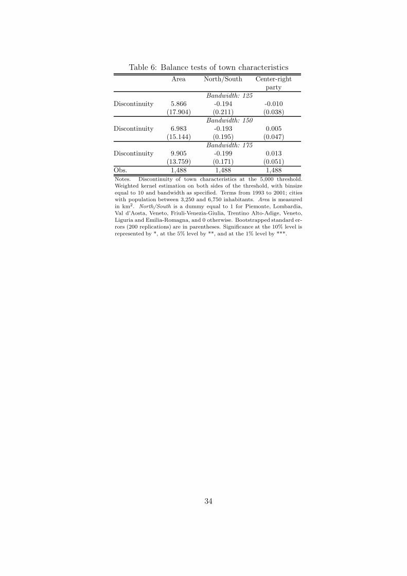
Table 6: Balance tests of town characteristics

Area North/South Center-rightparty

Bandwidth: 125

Discontinuity 5.866 -0.194 -0.010(17.904) (0.211) (0.038)

Bandwidth: 150

Discontinuity 6.983 -0.193 0.005(15.144) (0.195) (0.047)

Bandwidth: 175

Discontinuity 9.905 -0.199 0.013(13.759) (0.171) (0.051)

Obs. 1,488 1,488 1,488

Notes. Discontinuity of town characteristics at the 5,000 threshold.Weighted kernel estimation on both sides of the threshold, with binsize

equal to 10 and bandwidth as specified. Terms from 1993 to 2001; citieswith population between 3,250 and 6,750 inhabitants. Area is measured

in km2. North/South is a dummy equal to 1 for Piemonte, Lombardia,Val d’Aosta, Veneto, Friuli-Venezia-Giulia, Trentino Alto-Adige, Veneto,

Liguria and Emilia-Romagna, and 0 otherwise. Bootstrapped standard er-rors (200 replications) are in parentheses. Significance at the 10% level is

represented by *, at the 5% level by **, and at the 1% level by ***.

34

Table 7: Candidate selection, RDD estimates

Population Female Age Years of Not High-skilled Low-skilledschooling employed occupation occupation

LLR with optimal bandwidthEffect 0.005 -0.951 0.905*** -0.021 0.048 -0.018

(0.018) (0.608) (0.279) (0.024) (0.034) (0.025)∆ 1,300 1,600 900 1,000 1,500 1,400Obs. 4,805 5,953 3,295 3,758 5,581 5,191

LLR with half optimal bandwidthEffect 0.017 -0.664 1.012** -0.032 0.092* -0.043

(0.025) (0.848) (0.424) (0.034) (0.050) (0.035)∆ 650 800 450 500 750 700Obs. 2,373 3,064 1,637 1,851 2,728 2,575

Split polynomial approximationEffect -0.000 -0.257 1.205*** -0.047 0.162** -0.074

(0.030) (1.168) (0.415) (0.035) (0.067) (0.045)Obs. 6,544 6,544 6,544 6,544 6,544 6,544

Notes. Effect of the 33% wage increase at the 5,000 threshold on the characteristics of the three best candidates. Termsfrom 1993 to 2001. First estimate: Local Linear Regression (LLR) as in equation (6); the optimal symmetric bandwidth ∆

is chosen with cross-validation methods. Second estimate: LLR with half optimal bandwidth. Third estimate: 3rd orderpolynomial approximation on either side of the threshold as in equation (7); the maximum symmetric bandwidth is 1,750.

Age and Years of schooling are measured in years; the other variables are dummies. Not employed includes unemployed,retired, and any other individual out of the labor force. High-skilled occupation includes lawyers, professors, physicians, self-

employed, and entrepreneurs. Low-skilled occupation includes blue collars, clerks, and technicians. Other types of occupation

in the residual category. Standard errors robust to clustering at the municipality level are in parentheses. Significance atthe 10% level is represented by *, at the 5% level by **, and at the 1% level by ***.

35

Table 8: Mayor selection, RDD estimates

Population Female Age Years of Not High-skilled Low-skilledschooling employed occupation occupation

LLR with optimal bandwidthEffect -0.012 -0.746 0.879** 0.002 0.108 -0.035

(0.034) (1.127) (0.346) (0.031) (0.066) (0.035)∆ 800 900 1,100 1,200 800 1,400Obs. 1,340 1,531 1,905 2,053 1,340 2,396

LLR with half optimal bandwidthEffect 0.032 -0.485 1.174** -0.028 0.162* -0.062

(0.042) (1.658) (0.504) (0.043) (0.094) (0.050)∆ 400 450 550 600 400 700Obs. 692 759 913 999 692 1,187

Split polynomial approximationEffect 0.015 -0.006 1.633*** -0.057 0.217** -0.083

(0.043) (1.631) (0.558) (0.050) (0.090) (0.064)Obs. 3,039 3,039 3,039 3,039 3,039 3,039

Notes. Effect of the 33% wage increase at the 5,000 threshold on the characteristics of the elected mayor. Terms from 1993to 2001. First estimate: Local Linear Regression (LLR) as in equation (6); the optimal symmetric bandwidth ∆ is chosen

with cross-validation methods. Second estimate: LLR with half optimal bandwidth. Third estimate: 3rd order polynomialapproximation on either side of the threshold as in equation (7); the maximum symmetric bandwidth is 1,750. Age and

Years of schooling are measured in years; the other variables are dummies. Not employed includes unemployed, retired, andany other individual out of the labor force. High-skilled occupation includes lawyers, professors, physicians, self-employed,

and entrepreneurs. Low-skilled occupation includes blue collars, clerks, and technicians. Other types of occupation in the

residual category. Standard errors robust to clustering at the municipality level are in parentheses. Significance at the 10%level is represented by *, at the 5% level by **, and at the 1% level by ***.

36

Table 9: Candidate and mayor selection, robustness exercise

Population Female Age Years of Not High-skilled Low-skilledschooling employed occupation occupation

All candidates

LLR with optimal bandwidth and covariatesEffect 0.009 -0.931 0.846*** -0.017 0.035 -0.010

(0.017) (0.604) (0.271) (0.024) (0.034) (0.024)∆ 1,300 1,600 900 1,000 1,500 1,400Obs. 4,805 5,953 3,295 3,758 5,581 5,191

Mayors

LLR with optimal bandwidth and covariatesEffect -0.009 -0.730 0.796** 0.005 0.102 -0.028

(0.033) (1.117) (0.342) (0.031) (0.065) (0.035)∆ 800 900 1,100 1,200 800 1,400Obs. 1,340 1,531 1,905 2,053 1,340 2,396

Notes. Effect of the 33% wage increase at the 5,000 threshold on the characteristics of the three best candidates (toppanel) or of the elected mayor (bottom panel). Terms from 1993 to 2001. Local Linear Regression (LLR) as in equation

(6), with optimal bandwidth ∆ and invariant town characteristics (Area in km2 and North/South dummy) as additionalcovariates. Age and Years of schooling are measured in years; the other variables are dummies. Not employed includes

unemployed, retired, and any other individual out of the labor force. High-skilled occupation includes lawyers, professors,

physicians, self-employed, and entrepreneurs. Low-skilled occupation includes blue collars, clerks, and technicians. Othertypes of occupation in the residual category. Standard errors robust to clustering at the municipality level are in parentheses.

Significance at the 10% level is represented by *, at the 5% level by **, and at the 1% level by ***.

37

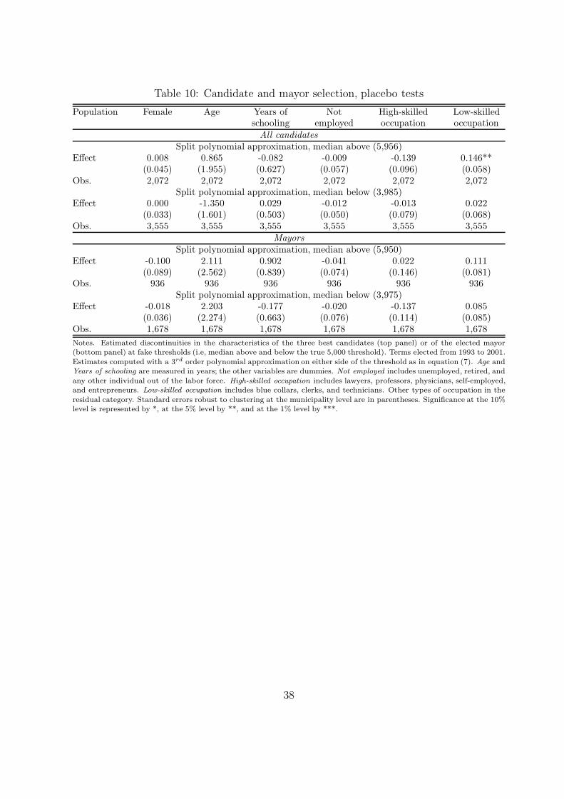
Table 10: Candidate and mayor selection, placebo tests

Population Female Age Years of Not High-skilled Low-skilledschooling employed occupation occupation

All candidates

Split polynomial approximation, median above (5,956)Effect 0.008 0.865 -0.082 -0.009 -0.139 0.146**

(0.045) (1.955) (0.627) (0.057) (0.096) (0.058)Obs. 2,072 2,072 2,072 2,072 2,072 2,072

Split polynomial approximation, median below (3,985)Effect 0.000 -1.350 0.029 -0.012 -0.013 0.022

(0.033) (1.601) (0.503) (0.050) (0.079) (0.068)Obs. 3,555 3,555 3,555 3,555 3,555 3,555

Mayors

Split polynomial approximation, median above (5,950)Effect -0.100 2.111 0.902 -0.041 0.022 0.111

(0.089) (2.562) (0.839) (0.074) (0.146) (0.081)Obs. 936 936 936 936 936 936

Split polynomial approximation, median below (3,975)Effect -0.018 2.203 -0.177 -0.020 -0.137 0.085

(0.036) (2.274) (0.663) (0.076) (0.114) (0.085)Obs. 1,678 1,678 1,678 1,678 1,678 1,678

Notes. Estimated discontinuities in the characteristics of the three best candidates (top panel) or of the elected mayor(bottom panel) at fake thresholds (i.e, median above and below the true 5,000 threshold). Terms elected from 1993 to 2001.

Estimates computed with a 3rd order polynomial approximation on either side of the threshold as in equation (7). Age andYears of schooling are measured in years; the other variables are dummies. Not employed includes unemployed, retired, and

any other individual out of the labor force. High-skilled occupation includes lawyers, professors, physicians, self-employed,and entrepreneurs. Low-skilled occupation includes blue collars, clerks, and technicians. Other types of occupation in the

residual category. Standard errors robust to clustering at the municipality level are in parentheses. Significance at the 10%level is represented by *, at the 5% level by **, and at the 1% level by ***.

38

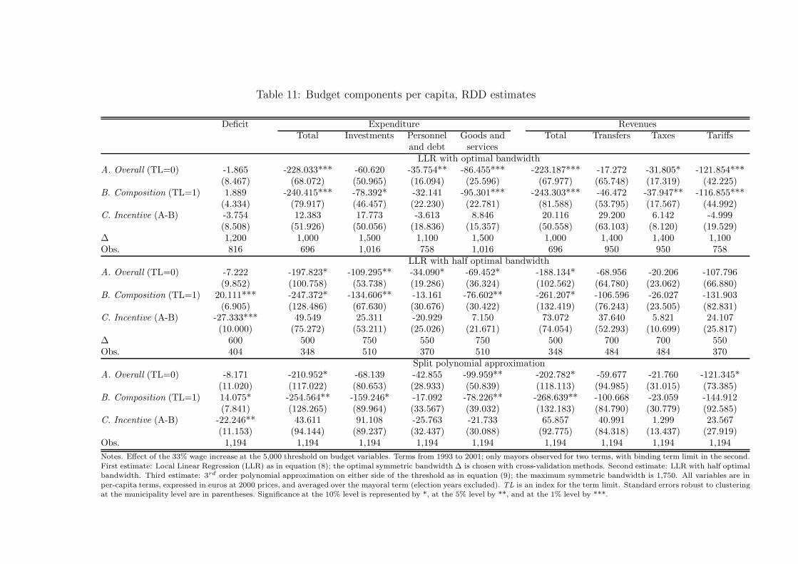
Table 11: Budget components per capita, RDD estimates

Deficit Expenditure RevenuesTotal Investments Personnel Goods and Total Transfers Taxes Tariffs

and debt servicesLLR with optimal bandwidth

A. Overall (TL=0) -1.865 -228.033*** -60.620 -35.754** -86.455*** -223.187*** -17.272 -31.805* -121.854***(8.467) (68.072) (50.965) (16.094) (25.596) (67.977) (65.748) (17.319) (42.225)

B. Composition (TL=1) 1.889 -240.415*** -78.392* -32.141 -95.301*** -243.303*** -46.472 -37.947** -116.855***(4.334) (79.917) (46.457) (22.230) (22.781) (81.588) (53.795) (17.567) (44.992)

C. Incentive (A-B) -3.754 12.383 17.773 -3.613 8.846 20.116 29.200 6.142 -4.999(8.508) (51.926) (50.056) (18.836) (15.357) (50.558) (63.103) (8.120) (19.529)

∆ 1,200 1,000 1,500 1,100 1,500 1,000 1,400 1,400 1,100Obs. 816 696 1,016 758 1,016 696 950 950 758

LLR with half optimal bandwidthA. Overall (TL=0) -7.222 -197.823* -109.295** -34.090* -69.452* -188.134* -68.956 -20.206 -107.796

(9.852) (100.758) (53.738) (19.286) (36.324) (102.562) (64.780) (23.062) (66.880)B. Composition (TL=1) 20.111*** -247.372* -134.606** -13.161 -76.602** -261.207* -106.596 -26.027 -131.903

(6.905) (128.486) (67.630) (30.676) (30.422) (132.419) (76.243) (23.505) (82.831)C. Incentive (A-B) -27.333*** 49.549 25.311 -20.929 7.150 73.072 37.640 5.821 24.107

(10.000) (75.272) (53.211) (25.026) (21.671) (74.054) (52.293) (10.699) (25.817)∆ 600 500 750 550 750 500 700 700 550Obs. 404 348 510 370 510 348 484 484 370

Split polynomial approximationA. Overall (TL=0) -8.171 -210.952* -68.139 -42.855 -99.959** -202.782* -59.677 -21.760 -121.345*

(11.020) (117.022) (80.653) (28.933) (50.839) (118.113) (94.985) (31.015) (73.385)B. Composition (TL=1) 14.075* -254.564** -159.246* -17.092 -78.226** -268.639** -100.668 -23.059 -144.912

(7.841) (128.265) (89.964) (33.567) (39.032) (132.183) (84.790) (30.779) (92.585)C. Incentive (A-B) -22.246** 43.611 91.108 -25.763 -21.733 65.857 40.991 1.299 23.567

(11.153) (94.144) (89.237) (32.437) (30.088) (92.775) (84.318) (13.437) (27.919)Obs. 1,194 1,194 1,194 1,194 1,194 1,194 1,194 1,194 1,194

Notes. Effect of the 33% wage increase at the 5,000 threshold on budget variables. Terms from 1993 to 2001; only mayors observed for two terms, with binding term limit in the second.

First estimate: Local Linear Regression (LLR) as in equation (8); the optimal symmetric bandwidth ∆ is chosen with cross-validation methods. Second estimate: LLR with half optimalbandwidth. Third estimate: 3rd order polynomial approximation on either side of the threshold as in equation (9); the maximum symmetric bandwidth is 1,750. All variables are in

per-capita terms, expressed in euros at 2000 prices, and averaged over the mayoral term (election years excluded). TL is an index for the term limit. Standard errors robust to clusteringat the municipality level are in parentheses. Significance at the 10% level is represented by *, at the 5% level by **, and at the 1% level by ***.

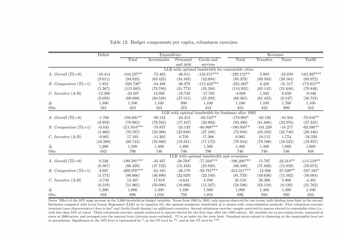
Table 12: Budget components per capita, robustness exercises

Deficit Expenditure RevenuesTotal Investments Personnel Goods and Total Transfers Taxes Tariffs

and debt servicesLLR with optimal bandwidth for contestable cities

A. Overall (TL=0) -10.414 -244.237** -72.462 -46.011 -133.215*** -229.152** 5.003 -22.859 -182.397***(9.011) (94.823) (63.425) (34.163) (42.694) (95.379) (69.563) (20.164) (68.072)

B. Composition (TL=1) 1.852 -220.730* -84.488 -26.279 -115.432*** -224.483* 3.420 -31.517 -172.851**(5.367) (112.085) (79.780) (31.773) (35.288) (114.922) (83.142) (21.648) (70.846)

C. Incentive (A-B) -12.266 -23.507 12.026 -19.733 -17.783 -4.669 1.583 8.659 -9.546(9.058) (69.898) (60.538) (37.515) (25.293) (68.365) (61.423) (9.547) (30.724)

∆ 1,400 1,100 1,100 900 1,100 1,100 1,100 1,700 1,100Obs. 581 453 453 373 453 453 453 699 453

LLR with optimal bandwidth for freshmen after 1993A. Overall (TL=0) -1.700 -194.691** -90.123 -24.413 -63.510** -179.994* -82.126 -16.504 -79.816**

(9.959) (78.982) (79.762) (17.447) (28.892) (93.490) (81.686) (22.076) (37.335)B. Composition (TL=1) -0.835 -211.854*** -78.857 -25.133 -80.898*** -186.958** -101.239 -18.277 -63.586**

(4.460) (70.767) (50.398) (22.939) (27.108) (72.858) (63.459) (22.740) (28.446)C. Incentive (A-B) -0.865 17.163 -11.265 0.720 17.388 6.965 19.113 1.774 -16.230

(10.208) (66.743) (76.860) (19.341) (17.172) (79.944) (79.586) (10.525) (19.827)∆ 1,200 1,500 1,400 1,400 1,500 1,400 1,400 1,000 1,600Obs. 642 796 746 746 796 746 746 546 848

LLR with optimal bandwidth and covariatesA. Overall (TL=0) 0.536 -199.591*** -45.437 -28.794* -77.334*** -196.206*** 15.797 -32.314** -115.519**

(8.587) (66.429) (47.732) (15.433) (25.928) (66.489) (57.826) (15.059) (50.073)B. Composition (TL=1) 3.807 -209.376*** -61.185 -26.179 -82.791*** -213.311*** -12.936 -37.828** -107.165*

(4.174) (80.066) (46.896) (22.029) (22.540) (81.733) (49.636) (15.502) (56.004)C. Incentive (A-B) -3.748 12.467 17.819 -3.644 8.709 20.158 29.396 5.988 -4.481

(8.519) (51.965) (50.096) (18.866) (15.347) (50.596) (63.158) (8.120) (21.762)∆ 1,200 1,000 1,500 1,100 1,500 1,000 1,400 1,400 1,100Obs. 816 696 1,016 758 1,016 696 950 950 624

Notes. Effect of the 33% wage increase at the 5,000 threshold on budget variables. Terms from 1993 to 2001; only mayors observed for two terms, with binding term limit in the second.Estimates computed with Local Linear Regression (LLR) as in equation (8); the optimal symmetric bandwidth ∆ is chosen with cross-validation methods. First robustness exercise:

invariant town characteristics (Area in km2 and North/South dummy) as additional covariates. Second robustness exercise: sample restricted to mayors elected in contestable cities (i.e.,with less than 55% of votes). Third robustness exercise: sample restricted to mayors elected for the first time after the 1993 reform. All variables are in per-capita terms, expressed in

euros at 2000 prices, and averaged over the mayoral term (election years excluded). TL is an index for the term limit. Standard errors robust to clustering at the municipality level arein parentheses. Significance at the 10% level is represented by *, at the 5% level by **, and at the 1% level by ***.

Table 13: Budget components per capita, placebo tests

Deficit Expenditure RevenuesTotal Investments Personnel Goods and Total Transfers Taxes Tariffs

and debt servicesSplit polynomial approximation, median above (5,932)

A. Overall (TL=0) 7.811 -160.051 -13.825 -21.167 -125.059 -167.863 -68.058 -74.455 -25.350(20.463) (228.821) (172.845) (69.780) (112.814) (228.685) (207.084) (68.814) (83.342)

B. Composition (TL=1) 11.548 -202.258 -4.351 -51.835 -146.071 -213.806 -85.559 -69.829 -58.418(12.891) (209.127) (99.392) (74.894) (92.317) (212.713) (159.264) (73.544) (68.603)

C. Incentive (A-B) -3.736 42.206 -9.474 30.668 21.012 45.943 17.501 -4.626 33.068(19.959) (193.491) (177.979) (54.873) (51.187) (194.461) (180.855) (38.430) (49.339)

Obs. 330 330 330 330 330 330 330 330 330Split polynomial approximation, median below (3,980)

A. Overall (TL=0) 17.094 149.264 146.787 44.621 -42.143 132.171 155.785 -39.932 16.317(12.782) (134.936) (100.112) (36.201) (44.314) (133.390) (125.144) (43.435) (46.820)

B. Composition (TL=1) 14.451 160.805 137.912 53.988 -31.094 146.354 180.280 -19.131 -14.795(8.936) (170.995) (131.895) (52.807) (45.590) (170.626) (170.028) (45.516) (32.712)

C. Incentive (A-B) -3.154 -122.480 -90.121 -22.168 -10.191 -119.325 -122.282 -21.435 24.393(13.711) (189.823) (184.674) (34.055) (32.993) (187.495) (187.477) (16.081) (27.119)

Obs. 666 666 666 666 666 666 666 666 666

Notes. Estimated discontinuities in budget components at fake thresholds (i.e, median above and below the true 5,000 threshold). Terms from 1993 to 2001; only mayors observed

for two terms, with binding term limit in the second. Estimates computed with a 3rd order polynomial approximation on either side of the threshold as in equation (9). Allvariables are in per-capita terms, expressed in euros at 2000 prices, and averaged over the mayoral term (election years excluded). TL is an index for the term limit. Standard

errors robust to clustering at the municipality level are in parentheses. Significance at the 10% level is represented by *, at the 5% level by **, and at the 1% level by ***.

Table 14: Efficiency measures, RDD estimates

Speed of Speed ofcollection payments

LLR with optimal bandwidthA. Overall (TL=0) 4.534* 1.636*

(2.482) (0.923)B. Composition (TL=1) 0.933 0.948

(2.742) (1.011)C. Incentive (A-B) 3.601 0.688

(3.597) (1.066)∆ 900 1,500Obs. 624 1,016

LLR with half optimal bandwidthA. Overall (TL=0) 5.565* 0.989

(3.217) (1.253)B. Composition (TL=1) -1.472 1.256

(4.378) (1.479)C. Incentive (A-B) 7.037 -0.267

(5.135) (1.406)∆ 450 750Obs. 328 510

Split polynomial approximationA. Overall (TL=0) 6.207* 0.986

(3.279) (1.661)B. Composition (TL=1) -1.604 0.747

(4.169) (1.987)C. Incentive (A-B) 7.811 0.238

(5.002) (1.819)Obs. 1,194 1,194

Notes. Effect of the 33% wage increase at the 5,000 threshold on efficiency measures.Terms from 1993 to 2001; only mayors observed for two terms, with binding term

limit in the second. First estimate: Local Linear Regression (LLR) as in equation (8);the optimal symmetric bandwidth ∆ is chosen with cross-validation methods. Second

estimate: LLR with half optimal bandwidth. Third estimate: 3rd order polynomial ap-proximation on either side of the threshold as in equation (9); the maximum symmetric

bandwidth is 1,750. The Efficiency measures are expressed in percentage points: Speedof collection is the ratio between collected and assessed revenues; Speed of payment is

the ratio between paid and committed outlays for public expenditure. TL is an indexfor the term limit. Standard errors robust to clustering at the municipality level are in

parentheses. Significance at the 10% level is represented by *, at the 5% level by **,and at the 1% level by ***.

42

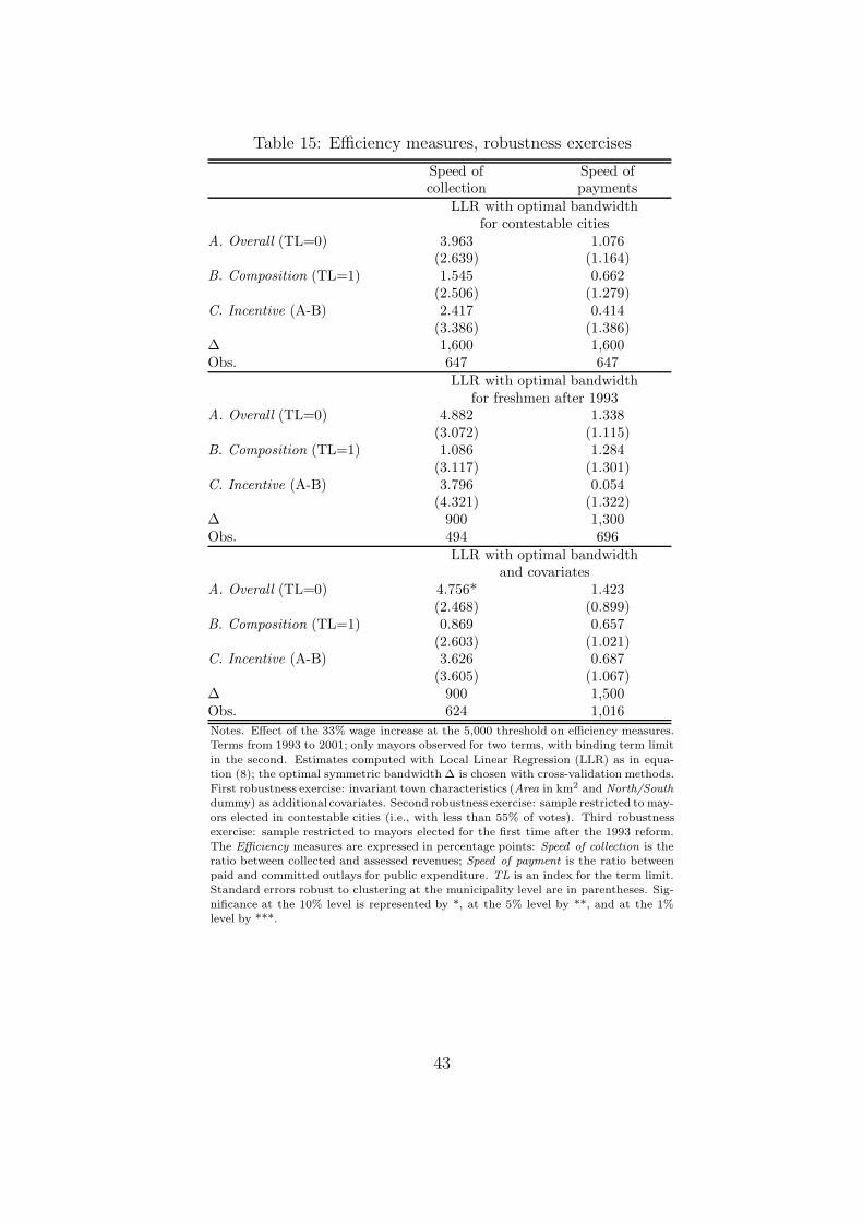
Table 15: Efficiency measures, robustness exercises

Speed of Speed ofcollection payments

LLR with optimal bandwidthfor contestable cities

A. Overall (TL=0) 3.963 1.076(2.639) (1.164)

B. Composition (TL=1) 1.545 0.662(2.506) (1.279)

C. Incentive (A-B) 2.417 0.414(3.386) (1.386)

∆ 1,600 1,600Obs. 647 647

LLR with optimal bandwidthfor freshmen after 1993

A. Overall (TL=0) 4.882 1.338(3.072) (1.115)

B. Composition (TL=1) 1.086 1.284(3.117) (1.301)

C. Incentive (A-B) 3.796 0.054(4.321) (1.322)

∆ 900 1,300Obs. 494 696

LLR with optimal bandwidthand covariates

A. Overall (TL=0) 4.756* 1.423(2.468) (0.899)

B. Composition (TL=1) 0.869 0.657(2.603) (1.021)

C. Incentive (A-B) 3.626 0.687(3.605) (1.067)

∆ 900 1,500Obs. 624 1,016

Notes. Effect of the 33% wage increase at the 5,000 threshold on efficiency measures.Terms from 1993 to 2001; only mayors observed for two terms, with binding term limit

in the second. Estimates computed with Local Linear Regression (LLR) as in equa-tion (8); the optimal symmetric bandwidth ∆ is chosen with cross-validation methods.

First robustness exercise: invariant town characteristics (Area in km2 and North/Southdummy) as additional covariates. Second robustness exercise: sample restricted to may-

ors elected in contestable cities (i.e., with less than 55% of votes). Third robustnessexercise: sample restricted to mayors elected for the first time after the 1993 reform.

The Efficiency measures are expressed in percentage points: Speed of collection is theratio between collected and assessed revenues; Speed of payment is the ratio between

paid and committed outlays for public expenditure. TL is an index for the term limit.Standard errors robust to clustering at the municipality level are in parentheses. Sig-

nificance at the 10% level is represented by *, at the 5% level by **, and at the 1%level by ***.

43

Table 16: Efficiency measures, placebo tests

Speed of Speed ofcollection payments

Split polynomial approximationmedian above (5,932)

A. Overall (TL=0) 2.208 4.102(5.098) (3.425)

B. Composition (TL=1) -0.823 0.827(7.891) (3.656)

C. Incentive (A-B) 3.031 3.274(9.314) (3.336)

Obs. 330 330

Split polynomial approximationmedian below (3,980)

A. Overall (TL=0) 1.589 -1.507(5.313) (2.076)

B. Composition (TL=1) -3.825 -2.125(3.661) (2.181)

C. Incentive (A-B) 4.068 0.042(6.203) (2.187)

Obs. 666 666

Notes. Estimated discontinuities in efficiency measures at fake thresholds (i.e, median

above and below the true 5,000 threshold). Terms from 1993 to 2001; only mayorsobserved for two terms, with binding term limit in the second. Estimates computed

with a 3rd order polynomial approximation on either side of the threshold as in equation(9). The Efficiency measures are expressed in percentage points: Speed of collection

is the ratio between collected and assessed revenues; Speed of payment is the ratiobetween paid and committed outlays for public expenditure. TL is an index for the term

limit. Standard errors robust to clustering at the municipality level are in parentheses.Significance at the 10% level is represented by *, at the 5% level by **, and at the 1%

level by ***.

44

Figure 1: Population distribution (<20,000)

1000

frequency

1000 3000 5000 10000 15000

population size

bin=500 bin=250

bin=100

Notes. Frequency of cities according to population in the 2001 Census. Citiesbelow 20,000 inhabitants only. Vertical lines identify policy thresholds.

Figure 2: Population density around the 5,000 threshold

25

50

frequency

4500 5000 5500

population size − 2001 Census

bin=200 bin=100

bin=50

Notes. Frequency of cities around the 5,000 threshold (vertical line), accordingto population size in the 2001 Census.

45

Figure 3: McCrary test

0.0002

.0004

.0006

3000 4000 5000 6000 7000

Notes. Weighted kernel estimation of the log density (according to the 2001Census), performed separately on either side of the 5,000 threshold. Optimalbinwidth and binsize as in McCrary (2008).

Figure 4: Candidate characteristics around the 5,000 threshold

.04.06.08

.1

.12.14

female

4600 4800 5000 5200 5400

population size

43

44

45

46

47

48

age

4600 4800 5000 5200 5400

population size

13.5

14

14.5

15

15.5

years of schooling

4600 4800 5000 5200 5400

population size

.05

.1

.15

.2

.25

not employed

4600 4800 5000 5200 5400

population size

.3

.4

.5

.6

.7

high−skilled

4600 4800 5000 5200 5400

population size

.05

.1

.15

.2

.25

.3

low−skilled

4600 4800 5000 5200 5400

population size

left right

fitted observed

Notes. The solid line is a running-mean smoothing of the variable on thevertical axis (with a bandwidth of 1), performed separately on either side ofthe 5,000 threshold. The dash line is a fitted regression over the whole sample.The dots are the observed values averaged in intervals of 50 inhabitants.

46

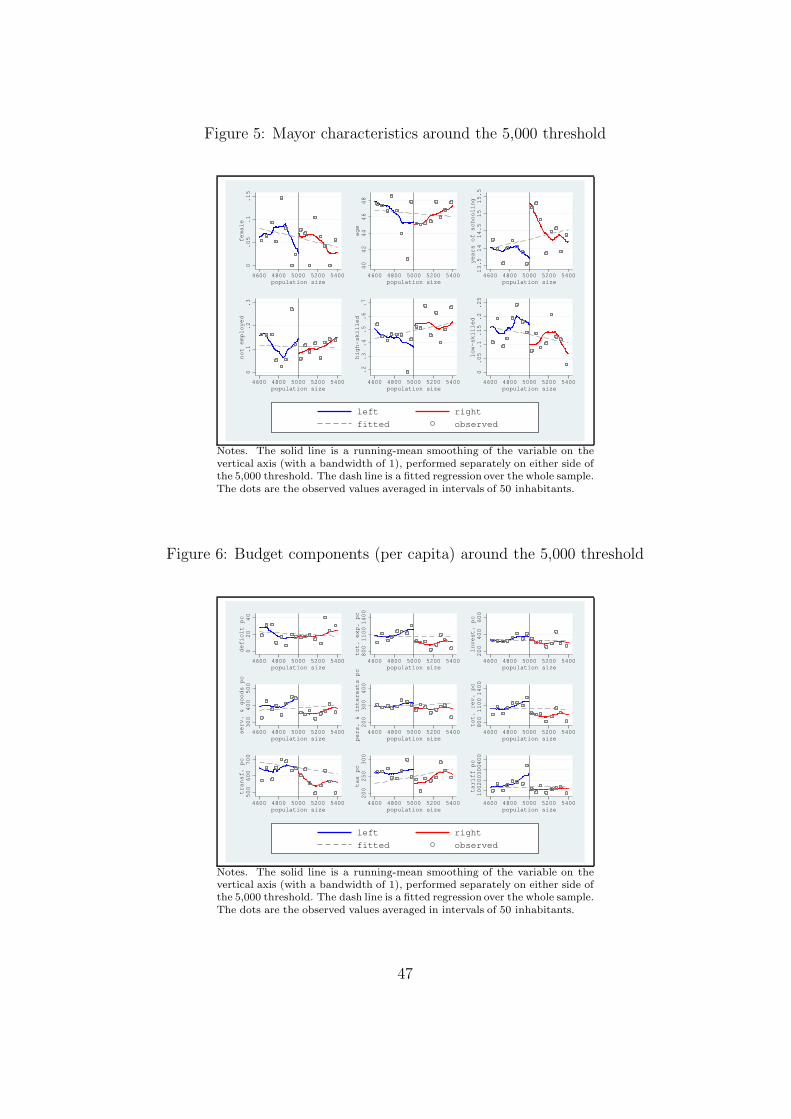
Figure 5: Mayor characteristics around the 5,000 threshold

0.05

.1

.15

female

4600 4800 5000 5200 5400

population size

40

42

44

46

48

age

4600 4800 5000 5200 5400

population size

13.5

14

14.5

15

15.5

years of schooling

4600 4800 5000 5200 5400

population size

0.1

.2

.3

not employed

4600 4800 5000 5200 5400

population size

.2

.3

.4

.5

.6

.7

high−skilled

4600 4800 5000 5200 5400

population size

0.05

.1

.15

.2

.25

low−skilled

4600 4800 5000 5200 5400

population size

left right

fitted observed

Notes. The solid line is a running-mean smoothing of the variable on thevertical axis (with a bandwidth of 1), performed separately on either side ofthe 5,000 threshold. The dash line is a fitted regression over the whole sample.The dots are the observed values averaged in intervals of 50 inhabitants.

Figure 6: Budget components (per capita) around the 5,000 threshold

020

40

deficit pc

4600 4800 5000 5200 5400

population size

800

11001400

tot. exp. pc

4600 4800 5000 5200 5400

population size

200

400

600

invest. pc

4600 4800 5000 5200 5400

population size

300

400

500

serv. & goods pc

4600 4800 5000 5200 5400

population size

200

300

400

pers. & interests pc

4600 4800 5000 5200 5400

population size

800

11001400

tot. rev. pc

4600 4800 5000 5200 5400

population size

500

600

700

transf. pc

4600 4800 5000 5200 5400

population size

200

250

300

tax pc

4600 4800 5000 5200 5400

population size

100200300400

tariff pc

4600 4800 5000 5200 5400

population size

left right

fitted observed

Notes. The solid line is a running-mean smoothing of the variable on thevertical axis (with a bandwidth of 1), performed separately on either side ofthe 5,000 threshold. The dash line is a fitted regression over the whole sample.The dots are the observed values averaged in intervals of 50 inhabitants.

47

Figure 7: Efficiency measures around the 5,000 threshold

60

65

70

75

Speed of collection

4600 4800 5000 5200 5400

population size

75

80

Speed of payment

4600 4800 5000 5200 5400

population size

left right

fitted observed

Notes. The solid line is a running-mean smoothing of the variable on thevertical axis (with a bandwidth of 1), performed separately on either side ofthe 5,000 threshold. The dash line is a fitted regression over the whole sample.The dots are the observed values averaged in intervals of 50 inhabitants.

48