districts “strawman” for considering further development ... · districts “strawman” for...

Districts “Strawman” for Considering Further Development of Unimpaired Hydrology for the

Tuolumne River in Advance of Workshop On March 27, 2013

1.0 Objective

Relicensing participants and the Districts are continuing to consider and discuss Tuolumne River

hydrology for use in the Tuolumne River Operations Model (W&AR-02). This draft report is intended to

be an initial “strawman” describing one possible approach to discuss further on March 27, 2013. The

objective of this particular “strawman” is to develop a daily flow dataset that contains no negative

values, results in more gradual changes in day-to-day flows, and conforms to the historical monthly

volumes previously recorded by the Districts and CCSF. The period of record under consideration is

Water Year 1971 – 2009. It is noted that the period of record may be extended to 2012 for use in the

development of the river and reservoir temperature models.

2.0 Background

On September 10, 2012, the California Department of Fish & Wildlife (CDFW), provided comments to

the State Water Resources Control Board (SWRCB) related to the unimpaired hydrology for the

operations/water balance model being developed for the Don Pedro Project relicensing. In summary,

CDFW is concerned “that the Districts’ proposed method of estimating unimpaired hydrology is not

appropriate for the purpose of the state of California’s environmental review process required for a new

license.”

The Districts subsequently undertook an investigation of CDFW’s suggested approach and submitted its

report to SWRCB, CDFW and FERC on December 21, 2012. This report was also provided as Attachment

A, Appendix A, of the W&AR-2 initial study report issued January 17, 2013. On February 14, 2013,

representatives from CDFW, SWRCB, and CCSF met with the Districts to discuss the Districts’ report and

the comparison of the two approaches. The Districts maintained that there was insufficient Tuolumne

River gauge data to support the gauge proration approach for the period of record of the Operations

Model. CDFW and SWRCB expressed interest in using all available gauge proration hydrology even if the

period of record was not as complete as might be desired. CDFW and SWRCB suggested that

alternatives be developed collaboratively in a workshop environment. CDFW and SWRCB agreed that

the monthly mass balance from the existing gauge summation hydrology was sound and need not be

adjusted. The Districts agreed to continue to discuss and consider alternative approaches, and agreed

to provide a “strawman” for to advance and promote dialogue at a meeting to be held on March 27.

3.0 Methods

Hydrologic input to the Operations Model currently includes daily unimpaired hydrology estimates for

three locations in the watershed: “La Grange” (at the USGS gage), “Hetch Hetchy Reservoir”, and Lake

Lloyd Reservoir/Lake Eleanor combined “Cherry/Eleanor”. The Operations Model uses these inputs to

calculate a fourth dataset of operational significance: the unimpaired flow from the unregulated portion

of the watershed above Don Pedro Reservoir (“Unregulated”). Details of these calculations are

described in the ISR of W&AR-2, Attachment A.

3.1 Gauge Proration “Strawman”

To promote and advance discussions for the March 27 Workshop, the Districts, as agreed with SWRCB,

CCSF and CDFW, have evaluated approaches to developing a hybrid flow record for the Tuolumne River

using a combination of gauge proration conforming to the existing monthly mass balances underlying

the Operations Model. This “strawman” is described below.

In order to prorate the gauged data to a larger ungauged area (application basin), three physical

variables were considered – elevation, drainage area, and average annual precipitation (precipitation).

Each gauged basin, along with each application basin (Hetch Hetchy, Cherry/Eleanor, and Unregulated),

was divided into 100-foot “elevation bands” for its entire drainage area. This was done using USGS

National Elevation Dataset, 1/3 arc-second (USGS, 2009), which equates to about a 30 foot pixel size.

Each elevation band for each gauge had attributes added for the drainage area within this band (e.g.,

the number of square miles of the Tuolumne River drainage that exists between elevation 500 and 600

feet) and precipitation (e.g. the average annual precipitation for the drainage area between elevation

500 and 600 feet).

The Oregon Climate Service’s PRISM model results were used to estimate average annual precipitation

from 1971 – 2000 (PRISM, 2006) for each of the elevation bands represented by the basins being

evaluated (elevation beginning 100 to 13,000 feet). PRISM uses the observed precipitation gauge and

radar data network, in conjunction with an orographic precipitation and atmospheric model, to develop

an estimate of average annual precipitation for the contiguous United States at a pixel size resolution of

2,500 feet. Bi-linear interpolation was used to resample the PRISM values to the same pixel size as the

elevation model.

Areas at low elevations and high elevations in each of the application basins that are poorly represented

or not represented at all by the reference gauges were “artificially added” into the elevation

distributions of the most representative gauges in order to provide some amount of coverage for those

elevation ranges. When artificial areas were added to the gauges, the amount of area added for each

gauge was nominally established as one percent of the total application basin area for that elevation

bin. For precipitation in artificially augmented elevation bands, a multiplier was applied to the

application basin precipitation values equal to the multiplier for the nearest observed elevation band for

that gauge.

The proration calculation includes two main steps. First, the daily flow for a given gauge is divided

across the elevation range that the gauge represents, in equal proportion to the drainage area

represented within each 100-foot elevation band. Second, the sum of each of the individual “elevation

band flows” for each gauge is scaled up to the area of that elevation band in the application basin. Each

of these steps includes a scaling factor for both area and precipitation. Equation 1 shows the calculation

for prorated flow on a single day, with the first step in the left set of parenthesis, and the second step in

the right set of parenthesis (mathematical summation form).

∑∑ ( ∑

)

( ∑

)

Equation 3.1.1 Daily unimpaired flow where is daily average flow, is area, and is average annual

precipitation. Where 𝑔 is each gauged basin, 𝑢 is the application basin, and 𝑒 is the lower limit of each

100-foot elevation band divided by 100.

It is worth noting here that a few of the reference gauge basins had facilities that resulted in measurable

amounts of stream regulation and/or diversion during the period of data use; no effort was made to

modify the observed data to account for these hydrologic effects. However, it is not expected that

these water regulation facilities would have a meaningful impact on the results of this analysis.

The following three sections of the “strawman” contain specific data to each application basin. Figure

3.1.1 shows where all the gauges used provide elevation coverage in reference to the application basin.

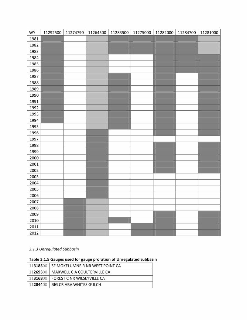
The first table in each subbasin description contains a list of gauges used for gauge proration hydrology

in that subbasin. The final table in each subbasin description shows gauge data availability from USGS,

where white is unavailable, light gray is available but not used, and dark gray means it is being used in

the subbasin gauge proration calculation. Some gauged data went unused when better gauged data

(closer, more similar in elevation range) were available.

Figure 3.1.1 Map of gauges used in proration method for unimpaired hydrology

3.1.1 Hetchy Hetchy Subbasin

Table 3.1.1 Gauges used for gauge proration of Hetch Hetchy subbasin

11292500 CLARK FORK STANISLAUS R NR DARDANELLE CA

11274790 TUOLUMNE R A GRAND CYN OF TUOLUMNE AB HETCH HETCHY

11264500 MERCED R A HAPPY ISLES BRIDGE NR YOSEMITE CA

11275000 FALLS C NR HETCH HETCHY

11282000 M TUOLUMNE R A OAKLAND RECREATION CAMP CA

Figure 3.1.2 Elevation histograms for unimpaired gauges, compared to the Hetch Hetchy subbasin

Table 3.1.2 Gauge inventory for gauge proration of Cherry/Eleanor subbasin

WY 11292500 11274790 11264500 11275000 11282000

1971 146

316 138

1972 114

269 104

1973 159

431 149

1974 202

454 184

1975 166

391 152

1976 66

135 62

1977 37

85 39

1978 179

576 215

0E+0

1E+5

2E+5

3E+5

4E+5

5E+5

6E+5

7E+5

8E+5

Dra

inag

e A

rea

in 1

00

ft

Ele

vati

on

Ban

d (

nu

mb

er

of

pix

els

)

Elevation (ft)

11292500

11274790

11264500

11275000

11282000

Hetch Hetchy

WY 11292500 11274790 11264500 11275000 11282000

1979 142

354 136

1980 232

529 172

1981 90

229 84

1982 280

640 272

1983 335

802 306

1984 224

449

121

1985 110

242

46

1986 230

539

129

1987 64

159

19

1988 60

208

22

1989 137

253

43

1990 75

174

27

1991 77

229

36

1992 65

200

22

1993 192

531

117

1994 73

163

19

1995

747

206

1996

438

98

1997

513 1998

594

182

1999

328

104

2000

331

89

2001

229

47

2002

299

59

2003

363 2004

256

2005

589 2006

638

2007

214 169 2008

292 268

2009

399 367

2010

492 392

2011

684 467 224

2012

228 31 44

3.1.2 Cherry/Eleanor Subbasin

Table 3.1.3 Gauges used for gauge proration of Cherry/Eleanor subbasin

11292500 CLARK FORK STANISLAUS R NR DARDANELLE CA

11274790 TUOLUMNE R A GRAND CYN OF TUOLUMNE AB HETCH HETCHY


11283500 CLAVEY R NR BUCK MEADOWS CA

11275000 FALLS C NR HETCH HETCHY


11284700 NF TUOLUMNE R NR LONG BARN CA

11281000 SF TUOLUMNE R NR OAKLAND RECREATION CAMP CA

Figure 3.1.3 Elevation histograms for unimpaired gauges, compared to the Cherry/Eleanor subbasin

Table 3.1.4 Gauge inventory for gauge proration of Cherry/Eleanor subbasin

WY 11292500 11274790 11264500 11283500 11275000 11282000 11284700 11281000

1971 147

237 138 65 25

1972 114

167 104 45 15

1973 159

287 149 86 28

1974 202

323 184 89 32

1975 166

314 152 97 36

1976 66

77 62 23 5

1977 37

31 39 6 2

1978 179

413 215 134 41

1979 142

278 136 90 29

1980 232

478 172 146 51

0E+0

1E+5

2E+5

3E+5

4E+5

5E+5

6E+5

7E+5

8E+5

Dra

inag

e A

rea

in 1

00

ft

Ele

vati

on

Ban

d (

nu

mb

er

of

pix

els

)

Elevation (ft)

11292500

11274790

11264500

11283500

11275000

11282000

11284700

11281000

Cherry/Eleanor

WY 11292500 11274790 11264500 11283500 11275000 11282000 11284700 11281000

1981 90

116 84 33 11

1982 280

606 272 168 62

1983 335

771 306 246 90

1984 224

121 39 140

1985 110

46 15 53

1986 230

129 52 164

1987 64

69

19

23

1988 60

82

22

26

1989 137

165

43

46

1990 75

97

27

35

1991 77

125

36

43

1992 65

100

22

31

1993 192

385

117

136

1994 73

86

19

28

1995

669

206

239

1996

438

98

126

1997

513 1998

594

182

206

1999

328

104

115

2000

331

89

105

2001

229

47

49

2002

299

59

51

2003

363 2004

256

2005

589 2006

638

2007

214 24 2008

292

2009

399

107

96

2010

492 398

97

65

2011

684

224 189

227

2012

228 14

44 41

6

3.1.3 Unregulated Subbasin

Table 3.1.5 Gauges used for gauge proration of Unregulated subbasin

11318500 SF MOKELUMNE R NR WEST POINT CA

11269300 MAXWELL C A COULTERVILLE CA

11316800 FOREST C NR WILSEYVILLE CA

11284400 BIG CR ABV WHITES GULCH

11283500 CLAVEY R NR BUCK MEADOWS CA



11284700 NF TUOLUMNE R NR LONG BARN CA

11281000 SF TUOLUMNE R NR OAKLAND RECREATION CAMP CA

Figure 3.1.4 Elevation histograms for unimpaired gauges, compared to the Unregulated subbasin

Table 3.1.6 Gauge inventory for gauge proration of Unregulated subbasin

WY 3185 2693 3168 2844 2835 2645 2820 2847 2810

1971 72 3 21 5 237 65 25 73

1972 38 2 13 2 167 45 15 51

1973 89 13 24 11 287 86 28 99

1974 105 9 31 8 323 89 32 103

1975 83

24 11 314 97 36 120

1976 15 1 5 1 77 23 5 25

1977 6 0 2 0 31 6 2 9

1978 112 18 28 14 413 134 41 167

1979 78 14 21 8 278 90 29 110

1980 138 17 39 17 478 146 51 182

1981 29

9 2 116 33 11 40

0E+0

1E+5

2E+5

3E+5

4E+5

5E+5

6E+5

7E+5

8E+5

9E+5

Dra

inag

e A

rea

in 1

00

ft

Ele

vati

on

Ban

d (

nu

mb

er

of

pix

els

)

Elevation (ft)

11318500

11269300

11316800

11284400

11283500

11264500

11282000

11284700

11281000

Unregulated

WY 3185 2693 3168 2844 2835 2645 2820 2847 2810

1982 194

48 20 606 168 62 196

1983 264

68 38 771 246 90 330

1984 111

34 14

449 121 39 140

1985 38

12 4

242 46 15 53

1986 150

40 20

539 129 52 164

1987 17

6 1 69 19

23

1988 10

4 0 82 22

26

1989 26

9 2 165 43

46

1990 20

7 1 97 27

35

1991 18

7 4 125 36

43

1992 19

6 3 100 22

31

1993 100

26 14 385 117

136

1994 16

5 1 86 19

28

1995 185

52 18 669 206

239

1996 97

27 12

438 98

126

1997 155

40 27

513 1998 163

45 22

594 182

206

1999 110

31 10

328 104

115

2000 89

23 12

331 89

105

2001 37

11 4

229 47

49

2002 46

14 3

299 59

51

2003 53

17 3

363 2004 39

12 3

256

2005 116

31 15

589 2006 184

55 20

638

2007 37

11 2

169 2008 30

8 4

268

2009 62

16 3

367 107

96

2010 68

18 7 398 95 97

101

2011 174

47 22

676 189

200

2012

3

194 41

52

3.2 Monthly Volume

In order to scale the gauge proration hydrology to the observed historical monthly volumes, some

adjustments had to be made to deal with months where the total monthly volume was calculated

negative. Negative monthly volumes in the current Tuolumne record are an artifact of gauge

summation calculations involving numerous flow and reservoir level gauges, each with small errors.

These calculations are described in detail in Attachment A of the ISR of W&AR-2. Negative monthly

volumes occur during certain low flow periods (August-January) of Cherry/Eleanor, Hetch Hetchy, and

unregulated inflow to Don Pedro. In total, adjustments were needed in 39 of the 504 months of the

extended period of record (WY 1971 – WY 2012). This resulted in small changes to the annual volume

from contributing subbasins for 22 of the 42 water years.

In order to eliminate negative monthly volumes without disturbing the gauge summation record, each

of the upper subbasins (Cherry/Eleanor and Hetch Hetchy) were re-balanced with the Unregulated

subbasin so that the monthly unimpaired volume at La Grange remains the same. Rather than

transferring just enough volume to ‘zero’ out the negative month, an attempt was made to use the

gauge proration record to find a reasonable value for the month being adjusted.

In the gauge proration hydrology record, typically the gauges being used don’t change during a water

year due to the way USGS reports data. Monthly volumes were examined as a percentage of the total

water year volume for both the gauge summation, and gauge proration data. The monthly percentage

of the annual volume was used as a guide to form an ‘expected’ monthly volume.

When the Unregulated subbasin had a negative month, Cherry/Eleanor and/or Hetch Hetchy volumes

for that month were examined for closeness to their ‘expected’ amount. In many cases, the

Cherry/Eleanor subbasin was far wetter than ‘expected’ and an adjustment down fixed a large portion of

the imbalance. In most cases, a blend of both Hetch Hetchy, and Cherry/Eleanor volumes were used to

offset a negative volume in the Unregulated subbasin. The exact percentage from each subbasin varies

depending on how the adjustment affected each subbasin.

When Cherry/Eleanor or Hetch Hetchy subbasins had a negative month, an ‘expected’ value was used as

a guide for the offset volume. All of the re-balancing volume came from the Unregulated subbasin. In

most cases, this volume had to be further adjusted manually in order to keep normal volumes in the

Unregulated subbasin. Table 3.2.1 shows these adjustments.

The only “new water” adjustment comes in October 2002, where 2000 AF was added to the La Grange

gauge. This was the minimum volume that could be used to produce a positive ‘expected normal’

month in the Unregulated subbasin (and Cherry/Eleanor subbasin). All of the adjustments made to the

Unregulated subbasin balance to a net of 2000 acre feet. In other words, for the period of record,

CCSF/Districts have the same amount of water flowing into the watersheds. The 2000 AF addition to La

Grange goes exclusively to the Unregulated subbasin.

Table 3.2.1 Adjustments to unregulated inflow volume to Don Pedro, in AF. Red indicates water going from the Unregulated subbasin to Cherry/Eleanor, orange to Hetch Hetchy, and green indicates water going from a combination of Cherry/Eleanor and Hetch Hetchy to the Unregulated subbasin.

WY Oct Nov Dec Jan Feb Mar Apr May Jun Jul Aug Sep

1971 -1,633

-3,369 -2,260

1972 -4,146

-3,024 -1,515

1973

-3,271 -4,695

1974

-4,741

1975 -3,518 1976

8,000


1977

-1,041

-1,359 7,287

1978 -1,545 1981 -6,652

1987

4,400

-400

1988

-800

1989

6,600 4,500 1990

3,088 3,600 2,800

1991 1,700

-1,500 1994

-7,923

-7,500 -981

1995 6,143 1996 2,400 -200

2000 -1,527

2003 4,400

2004 1,945 5,037

2007 4,200

2012 -500

Monthly scaling factors were used to scale the gauge proration hydrology up or down to the adjusted

historical monthly volume. The monthly scaling factor is defined as the adjusted historical monthly

volume divided by the gauge proration monthly volume. A scaling factor of less than one means the

gauge proration overestimated the historical flow. A scaling factor of greater than one means the gauge

proration underestimated the historical flow. When multiplied by the scaling factor, the daily gauge

proration flow values will result in adjusted historical monthly volumes. The following three sections

show computed scaling factors used for each subbasin, with red to orange indicating a reduction in

gauge proration flow, and yellow to green representing an increase in gauge proration flow.

3.2.1 Hetchy Hetchy Subbasin

Table 3.2.2 Hetch Hetchy monthly scaling factors for gauge proration. Bold indicates reduced volume and italics indicates increased volume.


1971 0.11 1.08 1.15 1.00 0.84 0.87 0.82 0.91 0.95 0.79 0.60 0.57

1972 0.48 0.75 1.04 0.98 0.96 0.82 0.81 0.89 0.84 0.56 0.32 0.27

1973 0.54 0.73 0.90 1.00 1.06 1.01 0.80 0.84 0.88 0.64 0.41 0.02

1974 0.32 0.87 1.02 0.94 0.72 0.88 0.79 0.83 0.87 0.85 0.57 0.07

1975 0.12 0.11 0.96 0.93 1.21 1.23 1.00 0.81 0.86 0.84 0.49 0.36

1976 0.81 0.87 0.74 0.05 0.98 0.94 0.83 0.93 0.82 0.71 0.70 0.44

1977 0.81 0.68 0.57 0.52 0.69 0.96 0.89 1.01 1.10 1.12 1.04 0.97

1978 0.52 0.96 1.25 1.67 1.67 1.15 0.91 0.79 0.88 1.03 0.73 0.64

1979 0.57 0.73 0.84 1.04 1.19 1.09 0.86 0.89 0.86 0.76 0.45 0.09

1980 0.82 0.92 0.83 1.03 0.98 0.93 0.80 0.80 1.00 1.18 0.84 0.36


1981 0.16 0.26 0.59 0.64 0.95 1.08 0.84 0.94 0.90 0.53 0.41 0.28

1982 0.91 1.09 1.03 1.09 0.94 0.78 0.74 0.81 0.89 0.87 0.86 0.91

1983 0.90 1.06 1.10 1.00 1.05 1.11 0.80 0.77 0.86 0.88 0.93 0.74

1984 0.95 1.80 1.45 0.96 1.06 1.17 1.22 1.58 1.76 1.24 0.79 0.60

1985 0.97 1.83 1.50 1.15 1.36 1.61 1.42 1.65 1.69 0.89 0.54 0.92

1986 1.55 1.63 2.13 1.90 1.57 1.19 1.27 1.45 1.62 1.56 1.01 0.57

1987 1.31 0.70 0.62 0.50 1.83 1.87 1.47 1.57 1.34 0.71 0.30 0.15

1988 0.56 1.10 1.77 2.03 1.43 1.40 1.55 1.59 1.40 0.80 0.55 0.57

1989 0.15 0.63 1.35 2.10 2.52 2.00 1.40 1.67 1.69 1.07 0.22 0.58

1990 1.34 1.41 1.50 2.03 2.14 1.81 1.58 1.61 1.50 0.76 0.39 0.12

1991 0.20 0.66 0.53 0.50 1.15 2.66 1.62 1.49 1.53 1.16 0.84 0.50

1992 1.18 1.39 1.35 1.44 2.02 1.70 1.39 1.37 1.00 1.02 0.74 0.61

1993 1.17 0.91 1.55 2.03 1.82 1.39 1.19 1.25 1.33 1.30 0.93 0.47

1994 0.88 0.56 1.28 0.62 1.84 2.08 1.64 1.70 1.64 0.62 2.06 0.61

1995 0.60 2.05 1.95 2.36 1.86 1.46 1.23 1.19 1.35 1.43 1.48 1.14

1996 0.39 0.95 1.91 1.74 1.78 1.34 1.30 1.47 1.84 1.70 1.05 1.01

1997 1.34 1.40 1.76 1.32 1.00 1.03 1.03 1.20 1.48 1.14 0.87 0.71

1998 1.03 1.17 1.96 2.49 1.72 1.58 1.19 1.23 1.34 1.35 0.87 0.77

1999 1.23 1.82 1.86 2.05 1.79 1.51 1.31 1.55 2.06 1.94 1.13 1.05

2000 1.54 1.61 1.26 2.42 1.98 1.54 1.45 1.49 1.50 1.17 1.11 0.92

2001 1.35 1.39 2.19 1.94 2.12 1.83 1.55 1.42 1.17 1.01 1.14 1.38

2002 2.46 1.71 2.09 1.81 1.67 1.51 1.40 1.57 1.61 1.13 1.22 2.06

2003 0.84 1.32 1.91 1.43 1.01 1.08 1.20 1.12 1.03 0.74 0.84 0.43

2004 1.27 1.26 1.90 0.89 0.95 1.20 1.22 1.40 1.33 0.88 0.96 1.55

2005 1.91 1.22 1.46 1.74 1.49 1.39 1.03 0.95 0.92 0.78 0.52 0.60

2006 0.88 1.09 2.14 1.23 1.24 1.14 1.06 0.99 1.10 0.88 0.56 0.27

2007 0.52 1.22 1.62 1.44 1.79 1.43 1.31 1.43 1.16 0.74 0.83 0.16

2008 1.28 1.32 1.90 1.52 1.58 1.36 1.26 1.36 1.32 0.83 0.48 0.77

2009 1.67 1.28 1.27 1.60 1.48 1.46 1.24 1.47 1.48 1.00 0.85 0.83

2010 1.31 1.03 1.52 1.56 1.57 1.52 1.49 1.36 1.31 1.06 0.75 1.06

2011 1.67 1.32 1.92 1.42 1.49 1.88 1.38 1.32 1.41 1.42 1.19 0.95

2012 1.02 0.92 0.58 1.38 1.18 1.30 1.32 1.28 1.07 0.69 0.58 0.61

3.2.2 Cherry/Eleanor Subbasin

Table 3.2.3 Cherry/Eleanor monthly scaling factors for gauge proration. Bold indicates reduced volume and italics indicates increased volume.


1971 0.52 2.91 2.04 1.66 1.42 1.46 1.37 1.47 1.37 1.00 0.52 0.52

1972 0.53 2.46 1.63 1.44 1.47 1.64 1.54 1.52 1.41 0.17 0.53 0.52

1973 0.67 1.80 2.11 1.48 1.15 1.19 1.43 1.45 1.30 0.44 0.49 0.49

1974 0.83 2.76 1.62 1.44 1.07 1.36 1.29 1.43 1.28 1.09 0.14 0.52

1975 0.48 0.23 1.52 1.75 1.37 1.38 1.39 1.46 1.28 1.16 0.42 0.39

1976 2.52 1.61 1.28 0.09 1.83 1.89 1.90 1.62 0.81 0.24 2.14 1.63

1977 1.65 0.82 0.71 1.57 2.40 2.38 2.16 2.25 1.48 0.14 0.72 1.80

1978 0.54 2.54 3.55 2.05 1.32 1.40 1.25 1.49 1.39 1.30 0.78 2.27


1979 0.05 1.27 1.78 2.10 1.62 1.41 1.51 1.44 1.28 0.99 1.15 1.62

1980 2.78 3.02 2.55 1.75 1.09 1.08 1.42 1.34 1.76 2.02 1.06 0.76

1981 0.62 0.44 1.61 1.65 2.28 1.85 1.98 1.66 1.36 1.27 3.38 2.36

1982 2.76 3.23 1.83 1.13 1.22 1.33 1.16 1.19 1.21 1.09 0.58 1.75

1983 2.39 1.52 1.03 0.96 0.91 0.84 0.99 1.27 1.27 1.32 1.21 1.07

1984 1.49 4.50 2.33 1.39 1.55 2.26 1.95 2.12 1.80 0.97 0.09 0.17

1985 2.47 5.03 3.28 2.01 2.66 3.12 2.95 2.43 1.91 0.81 0.92 1.16

1986 4.32 4.31 5.71 5.17 2.54 2.11 2.15 2.19 2.14 1.79 0.82 1.50

1987 1.38 0.71 0.98 0.67 3.76 3.25 3.89 2.65 1.66 0.36 0.76 0.63

1988 2.70 4.08 5.10 1.04 1.69 3.14 3.44 3.05 2.38 1.52 0.08 0.51

1989 1.27 4.80 4.05 4.02 3.73 3.25 2.30 2.36 2.02 0.52 0.09 3.64

1990 6.66 3.93 2.43 3.50 3.47 3.25 3.14 2.80 2.15 0.80 0.17 0.32

1991 0.47 0.67 0.92 1.02 2.53 5.29 3.43 3.01 2.68 2.25 0.84 0.24

1992 1.65 4.19 1.95 2.56 3.24 2.95 3.10 2.42 1.43 4.22 1.36 0.11

1993 3.35 3.58 3.09 2.44 1.74 2.08 2.02 2.11 2.20 2.36 1.09 0.40

1994 1.37 0.63 2.69 2.39 3.39 3.75 3.71 3.01 1.98 0.70 0.03 0.05

1995 1.79 11.40 4.67 1.83 2.07 1.28 1.80 1.96 2.01 1.64 1.38 0.35

1996 0.37 0.003 6.32 3.28 3.37 2.11 2.13 2.20 1.76 1.19 0.74 0.33

1997 2.40 3.24 5.53 2.56 1.70 2.05 1.69 1.14 1.06 0.52 0.24 1.27

1998 2.36 3.49 4.36 3.74 1.70 2.51 2.09 1.97 1.93 1.69 0.83 0.82

1999 1.13 5.78 3.78 3.34 2.36 2.49 2.28 2.25 2.27 1.52 0.30 0.04

2000 0.90 3.37 1.47 5.53 2.69 2.63 2.63 2.19 1.72 0.86 0.72 1.57

2001 3.18 4.09 5.20 5.25 5.16 4.28 2.84 1.78 0.92 1.02 3.35 3.66

2002 2.25 7.05 5.22 4.21 3.31 3.52 2.43 2.08 1.55 0.35 2.15 2.22

2003 1.43 4.70 6.20 4.35 2.99 3.03 2.24 1.42 0.99 0.63 1.18 2.60

2004 1.63 3.32 7.47 4.33 4.91 2.32 1.87 1.44 0.89 0.48 0.58 0.15

2005 7.77 4.56 5.68 4.44 3.54 2.79 1.99 1.64 1.21 0.85 0.27 0.84

2006 3.79 3.65 7.66 3.42 4.13 3.37 2.51 1.15 0.96 0.71 0.50 0.68

2007 2.07 5.46 7.26 6.35 6.84 3.92 2.59 1.74 1.11 1.68 4.46 2.06

2008 5.19 0.74 6.16 5.68 3.91 4.03 3.04 1.79 1.14 0.54 0.70 0.32

2009 2.78 4.80 3.51 5.02 4.01 3.55 2.93 2.61 2.19 1.08 1.02 1.47

2010 4.95 1.72 4.10 3.90 2.81 3.22 2.45 2.22 2.09 1.61 0.80 0.84

2011 4.61 4.01 3.06 2.60 2.86 2.26 2.46 2.51 1.78 1.66 1.71 1.71

2012 2.59 2.11 0.89 5.82 3.82 4.49 3.07 1.70 1.21 0.62 0.45 0.48

3.2.3 Unregulated Subbasin

Table 3.2.4 Unregulated subbasin scaling factors for gauge proration. Bold indicates reduced volume and italics indicates increased volume.


1971 2.11 1.73 1.42 1.31 1.01 0.92 0.84 0.85 0.93 1.38 1.51 1.48

1972 0.59 1.24 1.20 1.66 1.19 0.87 0.83 0.88 1.15 2.63 3.78 2.21

1973 1.18 1.98 1.45 1.27 1.43 1.27 0.84 0.78 1.15 1.89 1.99 1.52

1974 1.98 1.00 1.23 1.04 0.94 0.92 0.92 0.86 1.14 1.55 2.03 2.77

1975 2.45 1.39 1.24 1.33 1.60 1.30 1.07 0.70 0.81 0.88 1.73 1.77

1976 1.22 1.45 1.47 0.81 1.18 1.13 1.01 0.94 1.35 3.25 3.13 2.87


1977 1.47 1.62 0.39 1.45 1.14 0.95 0.86 0.96 1.03 0.40 2.77 1.02

1978 0.61 1.52 1.44 1.25 1.22 1.05 0.97 0.93 0.92 1.08 2.62 2.40

1979 1.22 2.85 1.45 1.46 1.50 1.17 0.83 0.79 0.96 1.60 1.52 1.79

1980 1.57 0.96 1.05 0.99 1.03 1.00 0.85 0.92 0.79 0.91 1.96 2.79

1981 1.48 0.90 1.56 1.76 0.93 1.40 0.83 0.89 1.40 2.88 8.09 3.69

1982 2.04 1.17 1.10 1.41 0.93 1.37 0.92 0.90 1.25 2.07 1.72 2.08

1983 1.09 1.16 1.01 1.22 1.13 1.05 0.97 0.79 0.75 0.90 0.92 1.12

1984 1.64 1.45 1.21 1.25 1.43 1.23 1.08 0.81 0.90 0.57 0.86 0.52

1985 1.22 1.49 1.15 1.06 1.40 1.62 1.07 0.81 0.73 1.25 3.49 2.36

1986 1.50 1.70 1.33 1.21 1.09 1.25 1.01 0.77 0.53 1.22 1.38 1.97

1987 1.19 0.65 0.77 0.37 1.12 1.30 0.73 0.81 1.64 1.87 3.59 0.66

1988 1.82 1.42 2.59 2.63 1.86 1.14 0.88 0.85 1.07 3.63 3.11 0.41

1989 0.56 2.05 1.65 1.45 1.16 0.94 0.78 0.77 0.94 0.71 0.86 0.64

1990 0.86 0.33 0.54 0.98 1.69 0.98 0.83 0.76 0.90 0.89 0.59 0.72

1991 0.14 3.34 0.86 1.39 1.18 1.59 0.98 0.94 1.00 3.28 6.76 5.02

1992 3.34 0.77 1.04 1.51 1.32 1.00 0.88 1.08 1.72 1.88 4.97 3.45

1993 2.13 0.40 1.49 1.50 1.31 0.94 0.76 0.76 0.89 1.54 2.77 2.74

1994 1.45 0.81 0.89 1.48 1.61 0.91 0.94 0.96 1.77 7.56 9.85 7.59

1995 0.40 1.06 1.77 1.28 0.96 1.10 0.95 0.89 0.92 0.94 0.85 0.70

1996 0.12 0.00 1.17 1.49 1.30 1.27 1.00 0.96 0.82 0.67 0.94 1.80

1997 0.90 1.44 1.44 1.22 1.04 1.41 1.07 0.74 0.25 0.77 1.77 1.18

1998 0.51 1.01 1.11 1.86 1.47 1.35 1.25 1.07 1.03 0.93 0.72 0.64

1999 0.39 1.00 1.13 1.31 1.17 1.09 1.11 0.97 1.02 1.25 1.65 2.27

2000 0.86 0.84 0.81 1.25 1.47 1.51 1.16 0.96 1.04 1.04 1.62 1.34

2001 1.23 0.54 0.85 1.22 1.46 1.33 1.11 0.86 0.85 1.51 2.39 2.60

2002 2.83 1.25 1.49 1.31 1.14 1.20 1.10 0.88 0.78 1.50 2.97 2.05

2003 0.16 1.16 1.51 0.94 0.93 1.19 0.92 0.76 0.56 0.66 1.75 1.75

2004 0.28 0.91 1.02 1.11 1.32 0.86 0.88 0.58 0.27 0.36 2.62 1.54

2005 2.52 0.52 1.14 1.61 1.43 1.25 1.10 1.09 0.99 0.84 1.36 2.22

2006 0.67 0.61 1.08 1.09 0.91 1.20 1.12 1.08 0.46 0.25 0.48 0.97

2007 0.92 0.57 0.68 0.18 1.19 0.79 0.82 0.47 0.42 0.68 0.75 0.55

2008 0.92 0.33 1.52 1.86 1.62 1.18 0.85 0.74 0.37 0.52 3.70 2.44

2009 0.24 0.88 0.81 1.74 1.20 0.99 0.83 0.80 0.55 1.00 2.01 1.73

2010 0.99 0.07 1.23 1.39 1.35 1.19 0.79 0.69 0.67 0.42 0.38 1.13

2011 1.01 1.28 1.32 1.25 1.20 1.27 1.03 0.76 0.82 0.69 0.96 1.00

2012 0.64 0.65 0.26 0.84 0.79 1.31 0.94 0.59 0.92 1.65 2.01 2.14

3.3 Smoothing Between Scaling Factors

It can be seen in the record of scaling factors that most of the period of record contains gradually

changing scaling factors each month. In several cases there are some abrupt changes, which have the

potential to artificially shape the gauge proration. This is particularly the case during snowmelt

recession, when a large factor in June might drop to a very small factor in July. This would make the

hydrograph appear to drop quite rapidly to the baseflow rate, instead of the expected gradual

recessional limb of a hydrograph.

In order to alleviate this problem, caused by the boundaries between monthly scaling factors, a

smoothing technique was used to gradually shift between scaling factors over the course of two weeks

(one week in each month). Any monthly volumetric changes resulting from this smoothing were applied

as a multiplier adjustment to the middle two weeks of the month. In most months, where scaling

factors do not change significantly, these adjustments do not change the hydrograph in any noticeable

way.

The function used to smooth between scaling factors was a cumulative normal distribution with a

standard deviation of 1.80. In several cases, in order to maintain the monthly volume, the standard

deviation had to be decreased in order to provide a more abrupt transition. An example of typical daily

scaling factors can be seen in Figure 3.3.1.

Figure 3.3.1 Typical daily scaling factor smoothing

4.0 Results

The resulting “strawman” can be seen in the attached HEC-DSS database.

5.0 Discussion

In water year 1997, and water years 2003-2008 there are only four unimpaired gauges representing the

Unregulated subbasin. Two of those gauges are in the Mokelumne River basin, one in the Merced River

basin, and the smallest one is in the Tuolumne River basin. Together, these four gauges provide a poor

representation of the Unregulated subbasin, and combined have a drainage area equal to less than 27%

of the Unregulated subbasin (Figure 5.1). This period is the poorest representation of any of the

application areas for the period of record. Despite the poor match in drainage size, elevation range, and

0.00

0.50

1.00

1.50

2.00

2.50

3.00

3.50

Mo

nth

ly S

calin

g Fa

cto

r

Hetch Hetchy

Cherry/Eleanor

Unregulated

even overall geography, the gauge proration provides a reasonable looking daily hydrograph when

scaled to the historical monthly volumes (Figure 5.2).

In the Operations Model, the function of the model is to allow comparisons to be made of different

scenarios. Absolute accuracy is not the goal. Relative differences between modeling scenarios is a

powerful decision making tool. While statistically accurate daily values may not be achieved using the

gauge proration methods described herein, they do create a dataset that:

Describes general hydrograph shape, variability, and magnitude of peak flows

Maintains the historical monthly volumes

Provides a reasonable depiction of daily flow conditions over the period of record

Figure 5.1 Elevation histogram for Unregulated subbasin gauge proration (WY 97, 02-08)

0E+0

1E+5

2E+5

3E+5

4E+5

5E+5

6E+5

7E+5

8E+5

9E+5

Dra

inag

e A

rea

in 1

00

ft

Ele

vati

on

Ban

d (

nu

mb

er

of

pix

els

)

Elevation (ft)

11318500

11316800

11284400

11264500

Unregulated

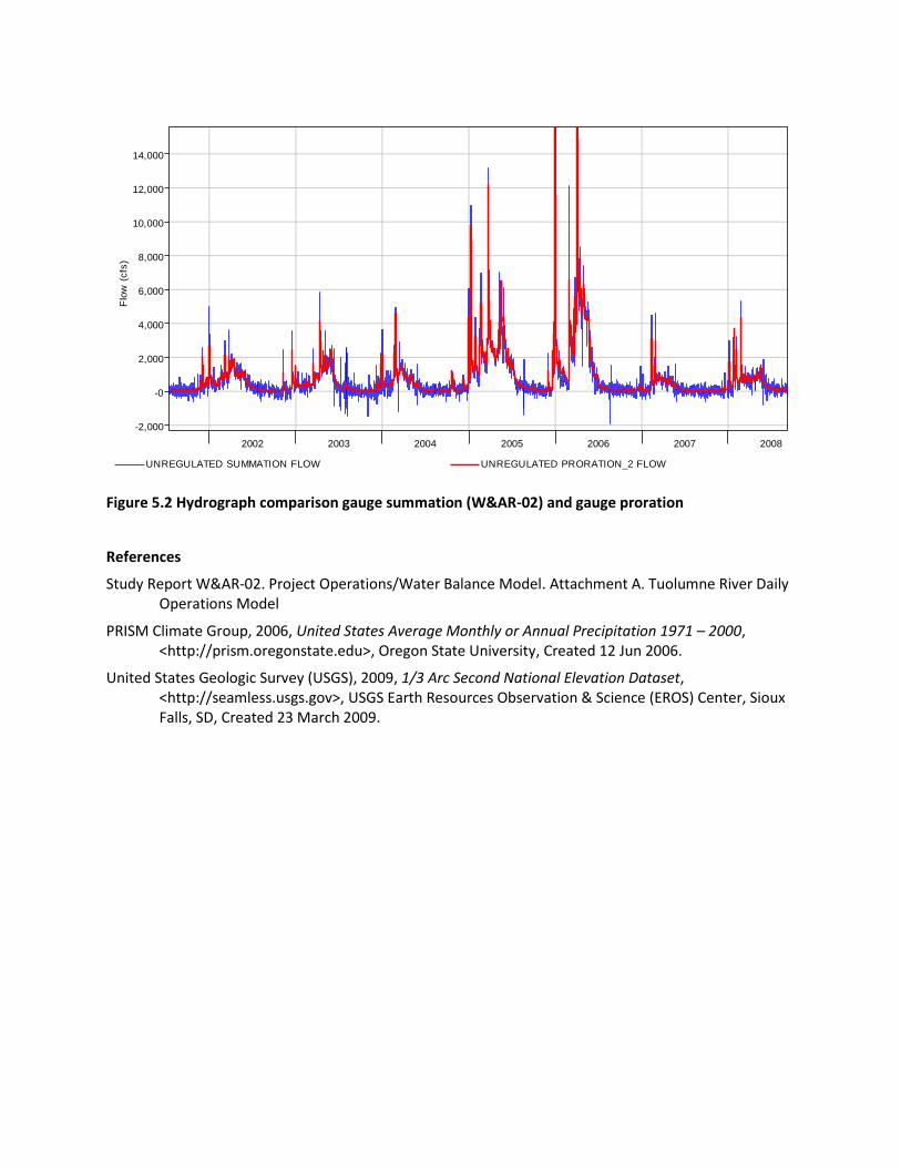
Figure 5.2 Hydrograph comparison gauge summation (W&AR-02) and gauge proration

References

Study Report W&AR-02. Project Operations/Water Balance Model. Attachment A. Tuolumne River Daily Operations Model

PRISM Climate Group, 2006, United States Average Monthly or Annual Precipitation 1971 – 2000, <http://prism.oregonstate.edu>, Oregon State University, Created 12 Jun 2006.

United States Geologic Survey (USGS), 2009, 1/3 Arc Second National Elevation Dataset, <http://seamless.usgs.gov>, USGS Earth Resources Observation & Science (EROS) Center, Sioux Falls, SD, Created 23 March 2009.

2002 2003 2004 2005 2006 2007 2008

Flo

w (

cfs

)

-2,000

-0

2,000

4,000

6,000

8,000

10,000

12,000

14,000

UNREGULATED SUMMATION FLOW UNREGULATED PRORATION_2 FLOW

districts “strawman” for considering further development ... · districts “strawman” for...

Documents