Distinct structural transitions of chromatin topological domains

coordinate hormone-induced gene regulation

François Le Dily1,2,3, Davide Baù1,3, Andy Pohl1,2, Guillermo Vicent1,2, François

Serra1,3, Daniel Soronellas1,2, Giancarlo Castellano1,2,4, Roni H.G. Wright1,2,

Cecilia Ballare1,2, Guillaume Filion1,2, Marc A. Marti-Renom1,3,5,* and Miguel

Beato1,2,*.

1 Gene Regulacion, Stem Cells and Cancer Program, Centre de Regulació

Genòmica (CRG), Barcelona, Spain

2 Universitat Pompeu Fabra (UPF), Barcelona, Spain

3 Genome Biology Group, Centre Nacional d’Anàlisi Genòmica (CNAG),

Barcelona, Spain

4 Hospital Clínic, Universitat de Barcelona, Barcelona, Spain

5 Institució Catalana de Recerca i Estudis Avançats (ICREA), Barcelona, Spain

*corresponding authors

Miguel Beato

E-mail: miguel.beato@crg.es

Centre de Regulació Genòmica

(CRG)

Dr. Aiguader 88,

E-08003, Barcelona, Spain.

Tel +34 93 316 0119

Fax +34 93 316 0099

Marc A. Marti-Renom

E-mail: mmarti@pcb.ub.cat

Centre Nacional d’Anàlisi Genòmica

(CNAG)

Baldiri i Reixac 4,

E-08028, Barcelona, Spain.

Tel. +34 934 020 542

Fax. +34 934 037 279

Keywords: Three-dimensional structure of the genome, gene expression, Hi-C,

TADs, transcriptional regulation, epigenetic landscape, progesterone receptor.

Running title: Hormone remodels specialized chromatin domains.

Supplementary Material

Table of contents

1. Supplementary Methods

1.1. Hi-C libraries, Reads mapping and filtering and generation of

Contact Matrices

1.2. Genome segmentation in TADs.

1.3. Epigenetic data collection and analysis

1.4. Role of TADs borders in the demarcation of chromatin blocs

1.5. Expression levels (RNA-Seq) and hormone induced changes

1.6. Classification of TAD according transcriptional response to Pg

1.7. Fluorescent In Situ Hybridization

1.8. Integrative modelling of spatial contacts

2. Supplementary Tables (Supplementary Tables 1-4)

3. Supplementary references

4. Supplementary Figures and legends (Supplementary Figures S1-S7)

1. Supplementary Methods

1.1. Hi-C libraries, reads mapping and filtering and generation of contact

matrices.

Hi-C libraries from T47D cells treated or not with the Pg analogue R5020 for 60

min were generated according the previously published Hi-C protocol with minor

adaptations (Lieberman-Aiden et al. 2009). Hi-C libraries were performed in both

conditions using HindIII and NcoI restriction enzymes to generate two

independent biological and technical replicates. Briefly, cells were fixed with 1%

formaldehyde during 10 min at room temperature. Cross-linking reactions were

stopped by addition of glycine (0.125 M final). Cells were scraped and nuclei

were prepared as described previously. Chromatin digestion, labelling and

ligation steps were performed according the original protocol (Lieberman-Aiden

et al. 2009). After deproteinisation, removal of biotinylated free-ends and DNA

purification, Hi-C libraries were controlled for quality and sequenced on an

Illumina Hiseq2000 sequencer. Paired-end reads were processed by first

aligning to the reference human genome (GRCh37/hg19) using BWA. Reads

filtered from the analysis include those that were not uniquely mapped, mapped

more than 500 bp from relevant internal restriction sites, had bad sequence

quality (e.g. 40% or more of the bases with Sanger PHRED quality ≤ 2) or bad

BWA mapping quality (≤ 20), or were located in regions classified to have

exceptionally high sequence depth (top 0.1%) by the 1000 Genomes project’s

data. To offset bias introduced by PCR amplification of the sequencing library,

only one of the duplicated pairs were used for subsequent analyses. Datasets

normalized for sequencing depth and experimental biases (Imakaev et al. 2012)

were used to generate contact matrices at 20, 40 and 100 Kb as well as at 1Mb

resolutions. The Supplementary table 1 summarizes the number of interactions

obtained for each dataset.

1.2. Genome segmentation in TADs.

The genome was segmented in TADs by the TADbit program that includes a

change-point algorithm for the detection of TAD borders inspired by methods

used to detect copy number variations in CGH experiments (Pique-Regi et al.

2008). Briefly, the optimal segmentation of the chromosome in k TADs is

computed by maximum likelihood for every k, after which a Bayesian

Information Criterion selects the best model. The hypotheses underlying the

model are that the number of interactions between two loci has a Poisson

distribution, of which the average decreases as a power law function of their

separation (in base pairs). Each TAD corresponds to a vertical slice of the Hi-C

interaction matrix, where the parameters of the model mentioned above are

constant. The parameters are corrected for local biases (most notably G+C

content, availability of the restriction enzyme site and repeat coverage)

(Imakaev et al. 2012). The detail of the implementation of TADbit will be further

detailed elsewhere (Serra et al., manuscript in preparation).

1.3. Epigenetic data collection and analyses.

MNase-seq, DNase I-seq and ChIP-seq experiments (H3K4me1, H3K4me3,

H2A, H4, RNA polymerase II, progesterone receptor, H3K9me3, HP1γ) in T47D

cells were described previously (Ballare et al. 2013; Vicent et al. 2013).

Additional ChIP-seq experiments for CTCF, H3K36me2, H3K27me3, H3K14ac

and H1.2 were performed in similar conditions using the following antibodies:

07-729 (Millipore), 07-369 (Millipore) 39155 (Active Motif), 07-353 (Millipore) and

ab4086 (Abcam), respectively. All reads were processed by aligning to the

reference human genome (GRCh37/hg19). MNase-seq, DNase I-seq and ChIP-

seq signals normalised for sequencing depth were summed in windows of 100

Kb. To generate plots in Supplementary Figures 2 and 3, bins correspond to a

fifth of the TAD size (hereafter mentioned as sub-segments). Summed reads for

these different window sizes were divided by the corresponding signal obtained

for an input DNA of T47D cells to determine the normalised signal over input

enrichment/depletion. Progesterone-induced enrichment or depletion of mark

content were determined for 100 Kb bins or for the whole TAD as the ratio of

sequencing-depth normalised read counts before and after treatment.

1.4. Role of TAD borders in demarking chromatin blocks.

To analyse the role of the TAD borders in limiting epigenetic blocks of individual

marks, the opposite of the absolute difference of the signals, normalised as

above, was calculated for two consecutive sub-segments (with each TAD

divided into 5 segments of equal size) on 3 consecutive TADs. Therefore, the

higher the score is, the more similar the signals between consecutive segments.

These scores were computed genome-wide, and the quartiles of the 14

consecutive values were calculated to generate the plots in Supplementary Fig.

3a and c. To control that the observed differences were not due to biases in the

sizes of the sub-segment, and to confirm the role of the TAD borders, we

shuffled the TADs chromosome-wise. As a robust control which conserves both

size and sequences of genomic domains, random segmentations of the

genome included inversion of the position of TADs from telomere to centromere

on each chromosomal arm (mentioned as random genomic domains (random

GD) in the main text and figures).

To analyse the homogeneity of epigenetic marks within TADs, we generated

pairwise correlation matrices between the profiles of the marks described above

for all 100 Kb windows of the genome. From this, we computed the average

correlation between 100 Kb windows located in the same TAD. If TADs are

homogeneous in chromatin marks combinations, this average correlation will be

higher than expected by chance. To estimate the null distribution of this score,

we shuffled the TADs chromosome-wise 5,000 times and applied the same

procedure. The average correlation obtained with the initial positions of the

TADs was higher than the average correlation when the TADs were

randomized. Finally, we repeated the same analysis using the differential of the

normalised signal after treatment with R5020 and the signal before treatment.

Borders of epigenetic domains were defined applying Principal Component

Analysis to the pair-wise correlation matrices of epigenetic profiles between 100

kb windows of the chromosomes obtained above. The number of those borders

that were located from 0 to 500 Kb from the TADs border were computed and

compared to random segmentation of the genome (see above).

1.5. Expression levels (RNA-seq) and hormone-induced changes.

RNA-seq experiments were performed in T47D treated or not with 10-8 M R5020

(Pg) for 1 or 6 h or with 10-8 M estradiol (E2) for 6 h. Paired-end reads were

mapped with the GEM mRNA Mapping Pipeline (v1.7) (Marco-Sola et al. 2012)

using the latest gencode annotation version (v.18) (Harrow et al. 2012). BAM

alignment files were obtained and used to generate strand-specific genome-

wide normalized profiles with RSeQC (Wang et al. 2012) software. Exon

quantifications summarized per gene for expression level determination were

obtained either as normalised read counts or reads per kilobase per milion

mapped reads (RPKM) using Flux Capacitor (Montgomery et al. 2010). Fold

changes (FC) were computed as the log2 ratio of normalised reads per gene

obtained after and before treatment with hormones. Genes with fold-change ±

1.5 (p-value < 0.05 ; FDR < 0.01) were considered as significantly regulated.

To analyse the changes of non-protein coding regions of the genome, the

number of normalised reads were computed independently for chromosomal

fractions of the TAD that do not overlap with any annotated protein-coding gene

and for chromosomal fractions of the TAD which contained protein-coding

reads.

In order to compare the observed and expected number of genes positively or

negatively affected by hormone treatment and to exclude potential biased

responses depending on low/high basal expression of genes, randomizations of

protein-coding gene positions used in Figure 2F were obtained as follow: genes

were classified in 5 classes of equivalent sizes according their expression level.

Gene positions were then shuffled for the 5 classes allowing conserving an

equivalent average expression of genes per TAD. Shuffled lists were then used

to calculate the percentage of genes with positive or negative fold change per

TAD and compared to the observed distribution.

1.6. Classification of TAD according transcriptional response to Pg.

To classify TADs according their hormone response, we calculated the average

ratio of the number of RNA-seq reads normalized for sequencing depth obtained

after and before hormone treatment in the RNA-seq replicates. TADs containing

more than 3 protein coding genes were saved for further analysis and ranked

according to the average ratio described above. The top and bottom 100 were

classified as “activated” and “repressed” TADs, respectively. Similar

classifications were performed for Pg and E2 response.

1.7. Fluorescent in situ hybridization.

T47D cells grown on slides were fixed with 4% paraformaldehyde in PBS 15 min

at room temperature. After washes with PBS and permeabilisation with 0.2%

Triton X-100 in PBS, slides were incubated 60 min with RNase A in SSC2X.

Fixed cells were incubated 3 min in 0.1 N HCl and 1 min in 0.01 N HCl with

0.01% pepsin. Slides were denatured at 70ºC for 8 min in SSC 2-70%

formamide and incubated overnight at 37ºC in a humid chamber with the probes

(separately denatured 10 min at 80ºC in hybridization buffer). 100 ng of each

probe generated by nick translation using dUTP-biotin, dUTP-DIG and dUTP-

fluorescein (Roche Applied Biosciences) was used per hybridization. Detection

was performed with ant-biotin-Cy5 (Rockland), anti-DIG-rhodamin (Roche) and

anti-fluorescein-Alexa 488 (Invitrogen). Machine optimized stacks were acquired

on a Zeiss TCS SP5 confocal microscope. After deconvolution, 3D rendering of

the hybridised probes signals were generated for each channel, and the pair-

wise 3D distances between the centre of mass of these signals were computed

using the Imaris Software.

The BACs used in this study were obtained from a 32k library:

RP11-758G19 chr1 : 26742822 - 26905278

RP11-443P17 chr1 : 26877973 - 27069024

RP11-973A19 chr1 : 27772963 - 27993702

RP11-667P18 chr1 : 28384701 - 28571122

RP11-318E23 chr1 : 28980912 - 29129694

RP11-476G18 chr2 : 43138737 - 43367330

RP11-525B14 chr2 : 43696249 - 43835952

RP11-4K20 chr2 : 11054580 - 11235239

RP11-345J13 chr2 : 11204622 - 11377387

RP11-487B6 chr2 : 11519339 - 11687756

RP11-641J22 chr2 : 11624003 - 11836772

1.8. Integrative 3D modelling of TADs.

Hi-C data matrices

Hi-C experimental data resulted in interaction counts between the loci of the

genomic region of interest (i.e. the quantitative determination of the number of

times each specific experimental ligation product is sequenced). We then

applied an internal normalization by Z-scoring the sequenced raw interaction

count data. First, we applied a log2 transformation of the raw counts and then

their Z-score was calculated as:

; where and are the average

and standard deviation of the interaction counts for the entire Hi-C matrix. Such

normalization allowed us to quantify the variability within the Hi-C matrix as well

as to identify pairs of fragments that significantly interacted above or below the

average interaction frequency.

TAD representation

Hi-C datasets obtained with HindIII and NcoI enzymes were pooled to generate

normalized Hi-C matrices at 20 Kb resolution. Consequently, each modelled

genomic region was represented as a set of particles, one per each 20 Kb bin.

Each particle had a radius of 100 nm, based on the relationship of 0.01 nm per

base pair (bp)(Harp et al. 2000). Neighbour particles were constrained to lie at

an equilibrium distance proportional to the sum of their excluded volume. Non-

neighbor particle pairs (i.e. particles representing non-consecutive bins along

the genomic sequence) were instead assigned a distance derived from the z-

score matrices. The function mapping the z-scores onto distances was defined

as the calibration curve built by interpolating the highest and the lowest z-score

values, with a minimum proximity distance of 200 nm (the excluded volume of

two base particles) and a maximal proximity distance for two non-interacting

fragments, respectively, as previously described (Bau and Marti-Renom 2012).

The forces applied to the defined restraints were also set proportionally to the

absolute value of the Hi-C z-score observed between a pair of fragments.

TAD modelling

Each particle pair was restrained by a series of harmonic oscillator centred on a

distance derived from the experimental data. Consecutive particles (i.e. particle

pairs —or bins— i, i+1) were considered as neighbour particles and therefore

retrained at an equilibrium distance proportional to the sum of their excluded

volume. Non-neighbour particles (i.e. particle pairs —or bins— i, i+2..n) were

instead restrained at distances calculated from a function that mapped their

corresponding z-scores onto distances. This function corresponded to a

calibration curve that was built between the points defined by the maximum and

minimum z-score values, and two empirically determined minimum and

maximum distances, respectively. The maximum distance for non-interacting

loci was independently optimized for each modelled region (Supplementary

Table 2). Consecutive particles were restrained by an upper-bound harmonic

oscillator, which ensured that two particles could not get separated beyond a

given equilibrium distance proportional to the sum of their excluded volume.

Non-consecutive particles were restrained by two different oscillators: (i) an

harmonic oscillator, which ensured a pair of particles to lie at about a given

equilibrium distance and (ii) lower-bound harmonic oscillator, which ensured that

two particles could not get closer than a given equilibrium distance. In both

cases the equilibrium distance was derived by a calibration curve defined by the

points corresponding to the maximum and minimum z-score values with a

minimum and a maximum distance (see below). The different type of oscillator

applied depended on an upper (uZ) and a lower (lZ) z-score cut-off as well as

the approximation distance between two non-interacting particles (aD), as

previously described (Bau and Marti-Renom 2012). The values of uZ, lZ and aD

were independently optimized for each modelled region (Supplementary Table

2).

Neighbour particles were constrained by an upper-bound harmonic oscillator

centered at an equilibrium distance proportional to the sum of their excluded

volume. Non-neighbour particles with a z-score higher than the upper-bound

cut-off (uZ) were restrained by a harmonic oscillator, while pairs of particles with

a z-score lower than the lower-bound cut-off (lZ) were restrained by a lower-

bound harmonic oscillator. Since these two harmonic oscillator aim at keeping a

pair of particles at an equilibrium distance or further apart from a minimal

distance, respectively, pairs of non-neighbour particles that were observed to

interact with z-scores above the uZ parameter were kept close in space, while

pairs of non-neighbor particles that were observed to interact with z-scores

below the lZ parameter were kept apart. The k force applied to these restraints

was set to the square root of the absolute value of their interacting z-scores.

Finally, pairs of non-neighbour particles for which Hi-C data were not available

were restrained based on the average z-score of the adjacent particles.

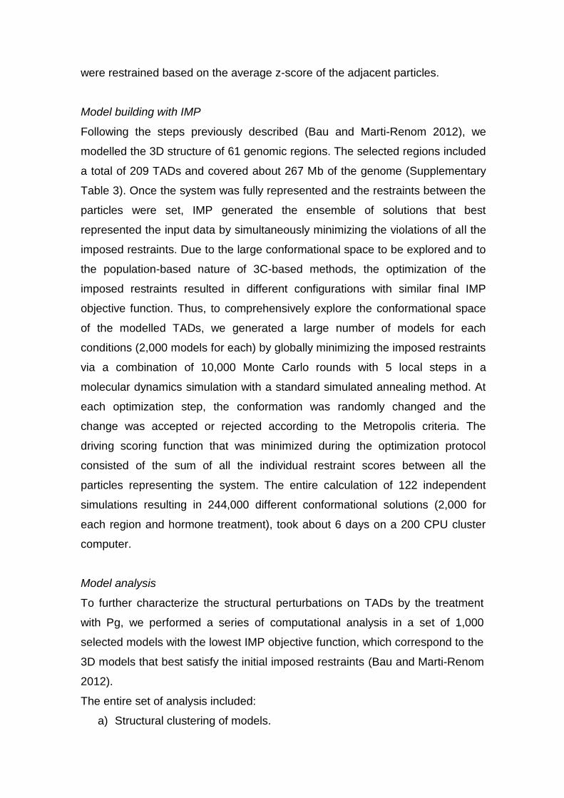
Model building with IMP

Following the steps previously described (Bau and Marti-Renom 2012), we

modelled the 3D structure of 61 genomic regions. The selected regions included

a total of 209 TADs and covered about 267 Mb of the genome (Supplementary

Table 3). Once the system was fully represented and the restraints between the

particles were set, IMP generated the ensemble of solutions that best

represented the input data by simultaneously minimizing the violations of all the

imposed restraints. Due to the large conformational space to be explored and to

the population-based nature of 3C-based methods, the optimization of the

imposed restraints resulted in different configurations with similar final IMP

objective function. Thus, to comprehensively explore the conformational space

of the modelled TADs, we generated a large number of models for each

conditions (2,000 models for each) by globally minimizing the imposed restraints

via a combination of 10,000 Monte Carlo rounds with 5 local steps in a

molecular dynamics simulation with a standard simulated annealing method. At

each optimization step, the conformation was randomly changed and the

change was accepted or rejected according to the Metropolis criteria. The

driving scoring function that was minimized during the optimization protocol

consisted of the sum of all the individual restraint scores between all the

particles representing the system. The entire calculation of 122 independent

simulations resulting in 244,000 different conformational solutions (2,000 for

each region and hormone treatment), took about 6 days on a 200 CPU cluster

computer.

Model analysis

To further characterize the structural perturbations on TADs by the treatment

with Pg, we performed a series of computational analysis in a set of 1,000

selected models with the lowest IMP objective function, which correspond to the

3D models that best satisfy the initial imposed restraints (Bau and Marti-Renom

2012).

The entire set of analysis included:

a) Structural clustering of models.

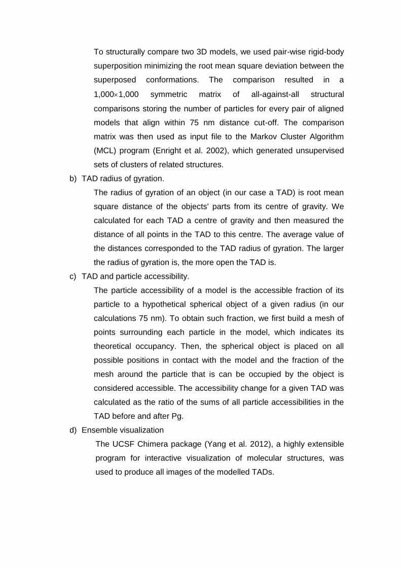
To structurally compare two 3D models, we used pair-wise rigid-body

superposition minimizing the root mean square deviation between the

superposed conformations. The comparison resulted in a

1,0001,000 symmetric matrix of all-against-all structural

comparisons storing the number of particles for every pair of aligned

models that align within 75 nm distance cut-off. The comparison

matrix was then used as input file to the Markov Cluster Algorithm

(MCL) program (Enright et al. 2002), which generated unsupervised

sets of clusters of related structures.

b) TAD radius of gyration.

The radius of gyration of an object (in our case a TAD) is root mean

square distance of the objects' parts from its centre of gravity. We

calculated for each TAD a centre of gravity and then measured the

distance of all points in the TAD to this centre. The average value of

the distances corresponded to the TAD radius of gyration. The larger

the radius of gyration is, the more open the TAD is.

c) TAD and particle accessibility.

The particle accessibility of a model is the accessible fraction of its

particle to a hypothetical spherical object of a given radius (in our

calculations 75 nm). To obtain such fraction, we first build a mesh of

points surrounding each particle in the model, which indicates its

theoretical occupancy. Then, the spherical object is placed on all

possible positions in contact with the model and the fraction of the

mesh around the particle that is can be occupied by the object is

considered accessible. The accessibility change for a given TAD was

calculated as the ratio of the sums of all particle accessibilities in the

TAD before and after Pg.

d) Ensemble visualization

The UCSF Chimera package (Yang et al. 2012), a highly extensible

program for interactive visualization of molecular structures, was

used to produce all images of the modelled TADs.

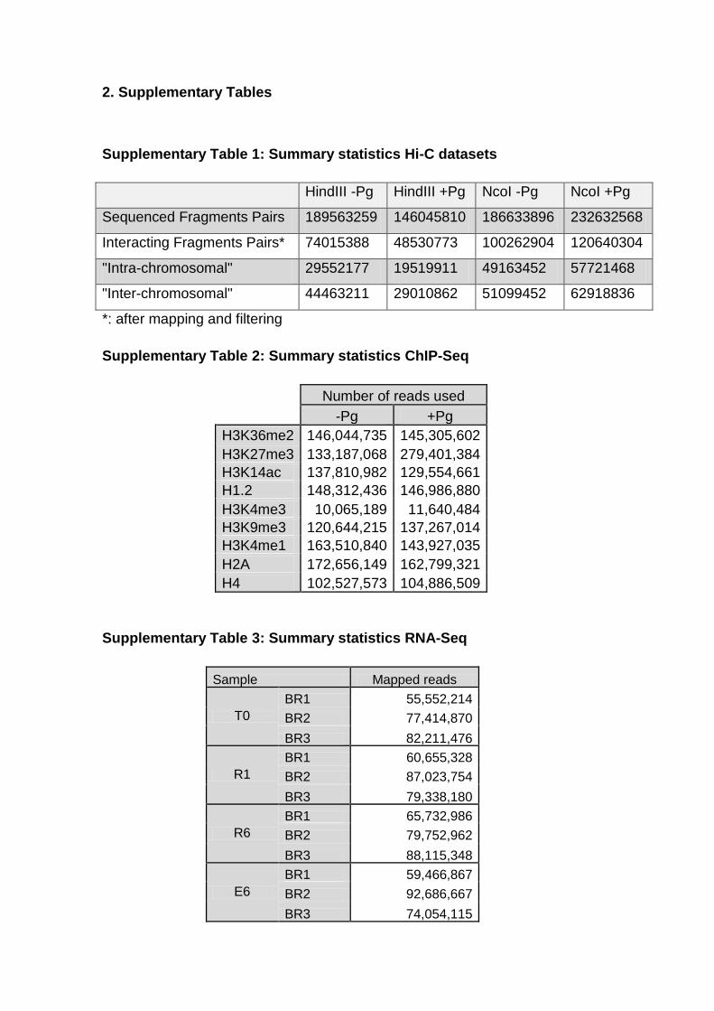
2. Supplementary Tables

Supplementary Table 1: Summary statistics Hi-C datasets

HindIII -Pg HindIII +Pg NcoI -Pg NcoI +Pg

Sequenced Fragments Pairs 189563259 146045810 186633896 232632568

Interacting Fragments Pairs* 74015388 48530773 100262904 120640304

"Intra-chromosomal" 29552177 19519911 49163452 57721468

"Inter-chromosomal" 44463211 29010862 51099452 62918836

*: after mapping and filtering

Supplementary Table 2: Summary statistics ChIP-Seq

Number of reads used

-Pg +Pg

H3K36me2 146,044,735 145,305,602

H3K27me3 133,187,068 279,401,384

H3K14ac 137,810,982 129,554,661

H1.2 148,312,436 146,986,880

H3K4me3 10,065,189 11,640,484

H3K9me3 120,644,215 137,267,014

H3K4me1 163,510,840 143,927,035

H2A 172,656,149 162,799,321

H4 102,527,573 104,886,509

Supplementary Table 3: Summary statistics RNA-Seq

Sample Mapped reads

T0

BR1 55,552,214

BR2 77,414,870

BR3 82,211,476

R1

BR1 60,655,328

BR2 87,023,754

BR3 79,338,180

R6

BR1 65,732,986

BR2 79,752,962

BR3 88,115,348

E6

BR1 59,466,867

BR2 92,686,667

BR3 74,054,115

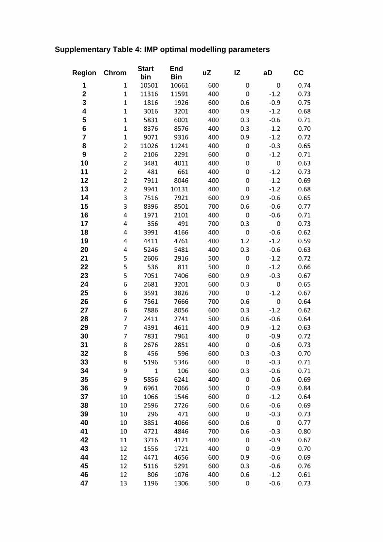
Supplementary Table 4: IMP optimal modelling parameters

Region Chrom Start bin

End Bin

uZ lZ aD CC

1 1 10501 10661 600 0 0 0.74 2 1 11316 11591 400 0 -1.2 0.73 3 1 1816 1926 600 0.6 -0.9 0.75 4 1 3016 3201 400 0.9 -1.2 0.68 5 1 5831 6001 400 0.3 -0.6 0.71 6 1 8376 8576 400 0.3 -1.2 0.70 7 1 9071 9316 400 0.9 -1.2 0.72 8 2 11026 11241 400 0 -0.3 0.65 9 2 2106 2291 600 0 -1.2 0.71 10 2 3481 4011 400 0 0 0.63 11 2 481 661 400 0 -1.2 0.73 12 2 7911 8046 400 0 -1.2 0.69 13 2 9941 10131 400 0 -1.2 0.68 14 3 7516 7921 600 0.9 -0.6 0.65 15 3 8396 8501 700 0.6 -0.6 0.77 16 4 1971 2101 400 0 -0.6 0.71 17 4 356 491 700 0.3 0 0.73 18 4 3991 4166 400 0 -0.6 0.62 19 4 4411 4761 400 1.2 -1.2 0.59 20 4 5246 5481 400 0.3 -0.6 0.63 21 5 2606 2916 500 0 -1.2 0.72 22 5 536 811 500 0 -1.2 0.66 23 5 7051 7406 600 0.9 -0.3 0.67 24 6 2681 3201 600 0.3 0 0.65 25 6 3591 3826 700 0 -1.2 0.67 26 6 7561 7666 700 0.6 0 0.64 27 6 7886 8056 600 0.3 -1.2 0.62 28 7 2411 2741 500 0.6 -0.6 0.64 29 7 4391 4611 400 0.9 -1.2 0.63 30 7 7831 7961 400 0 -0.9 0.72 31 8 2676 2851 400 0 -0.6 0.73 32 8 456 596 600 0.3 -0.3 0.70 33 8 5196 5346 600 0 -0.3 0.71 34 9 1 106 600 0.3 -0.6 0.71 35 9 5856 6241 400 0 -0.6 0.69 36 9 6961 7066 500 0 -0.9 0.84 37 10 1066 1546 600 0 -1.2 0.64 38 10 2596 2726 600 0.6 -0.6 0.69 39 10 296 471 600 0 -0.3 0.73 40 10 3851 4066 600 0.6 0 0.77 41 10 4721 4846 700 0.6 -0.3 0.80 42 11 3716 4121 400 0 -0.9 0.67 43 12 1556 1721 400 0 -0.9 0.70 44 12 4471 4656 600 0.9 -0.6 0.69 45 12 5116 5291 600 0.3 -0.6 0.76 46 12 806 1076 400 0.6 -1.2 0.61 47 13 1196 1306 500 0 -0.6 0.73

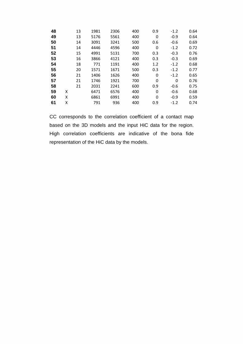
48 13 1981 2306 400 0.9 -1.2 0.64 49 13 5176 5561 400 0 -0.9 0.64 50 14 3091 3241 500 0.6 -0.6 0.69 51 14 4446 4596 400 0 -1.2 0.72 52 15 4991 5131 700 0.3 -0.3 0.76 53 16 3866 4121 400 0.3 -0.3 0.69 54 18 771 1191 400 1.2 -1.2 0.68 55 20 1571 1671 500 0.3 -1.2 0.77 56 21 1406 1626 400 0 -1.2 0.65 57 21 1746 1921 700 0 0 0.76 58 21 2031 2241 600 0.9 -0.6 0.75 59 X 6471 6576 400 0 -0.6 0.68 60 X 6861 6991 400 0 -0.9 0.59 61 X 791 936 400 0.9 -1.2 0.74

CC corresponds to the correlation coefficient of a contact map

based on the 3D models and the input HiC data for the region.

High correlation coefficients are indicative of the bona fide

representation of the HiC data by the models.

3. Supplementary References

Ballare C, Castellano G, Gaveglia L, Althammer S, Gonzalez-Vallinas J, Eyras E, Le Dily F, Zaurin R, Soronellas D, Vicent GP et al. 2013. Nucleosome-driven transcription factor binding and gene regulation. Molecular cell 49: 67-79.

Bau D, Marti-Renom MA. 2012. Genome structure determination via 3C-based data integration by the Integrative Modeling Platform. Methods 58: 300-306.

Enright AJ, Van Dongen S, Ouzounis CA. 2002. An efficient algorithm for large-scale detection of protein families. Nucleic acids research 30: 1575-1584.

Harp JM, Hanson BL, Timm DE, Bunick GJ. 2000. Asymmetries in the nucleosome core particle at 2.5 A resolution. Acta crystallographica Section D, Biological crystallography 56: 1513-1534.

Harrow J, Frankish A, Gonzalez JM, Tapanari E, Diekhans M, Kokocinski F, Aken BL, Barrell D, Zadissa A, Searle S et al. 2012. GENCODE: the reference human genome annotation for The ENCODE Project. Genome research 22: 1760-1774.

Imakaev M, Fudenberg G, McCord RP, Naumova N, Goloborodko A, Lajoie BR, Dekker J, Mirny LA. 2012. Iterative correction of Hi-C data reveals hallmarks of chromosome organization. Nature methods 9: 999-1003.

Lieberman-Aiden E, van Berkum NL, Williams L, Imakaev M, Ragoczy T, Telling A, Amit I, Lajoie BR, Sabo PJ, Dorschner MO et al. 2009. Comprehensive mapping of long-range interactions reveals folding principles of the human genome. Science 326: 289-293.

Marco-Sola S, Sammeth M, Guigo R, Ribeca P. 2012. The GEM mapper: fast, accurate and versatile alignment by filtration. Nature methods 9: 1185-1188.

Montgomery SB, Sammeth M, Gutierrez-Arcelus M, Lach RP, Ingle C, Nisbett J, Guigo R, Dermitzakis ET. 2010. Transcriptome genetics using second generation sequencing in a Caucasian population. Nature 464: 773-777.

Pique-Regi R, Monso-Varona J, Ortega A, Seeger RC, Triche TJ, Asgharzadeh S. 2008. Sparse representation and Bayesian detection of genome copy number alterations from microarray data. Bioinformatics 24: 309-318.

Vicent GP, Nacht AS, Zaurin R, Font-Mateu J, Soronellas D, Le Dily F, Reyes D, Beato M. 2013. Unliganded progesterone receptor-mediated targeting of an RNA-containing repressive complex silences a subset of hormone-inducible genes. Genes & development 27: 1179-1197.

Wang L, Wang S, Li W. 2012. RSeQC: quality control of RNA-seq experiments. Bioinformatics 28: 2184-2185.

Yang Z, Lasker K, Schneidman-Duhovny D, Webb B, Huang CC, Pettersen EF, Goddard TD, Meng EC, Sali A, Ferrin TE. 2012. UCSF Chimera, MODELLER, and IMP: an integrated modeling system. Journal of structural biology 179: 269-278.

4. Supplementary Figures and legends

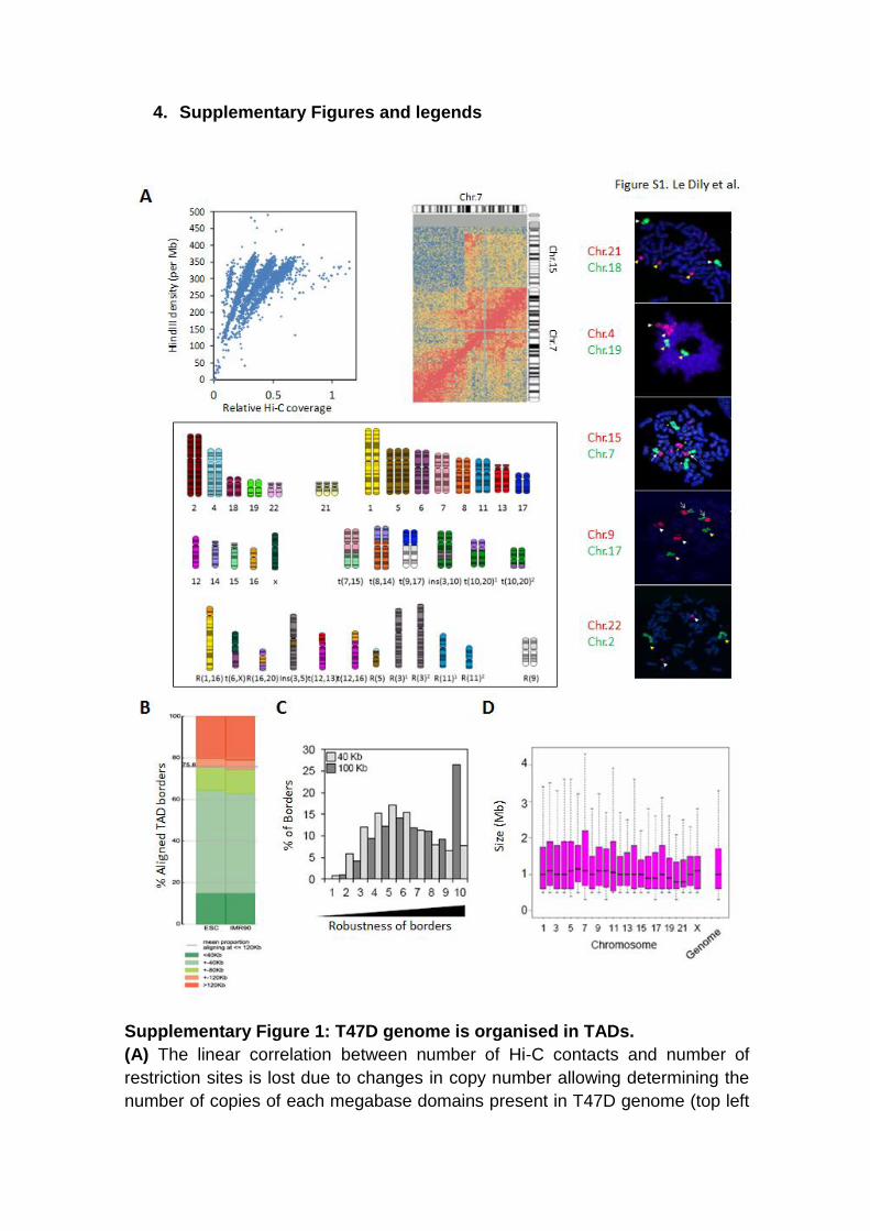
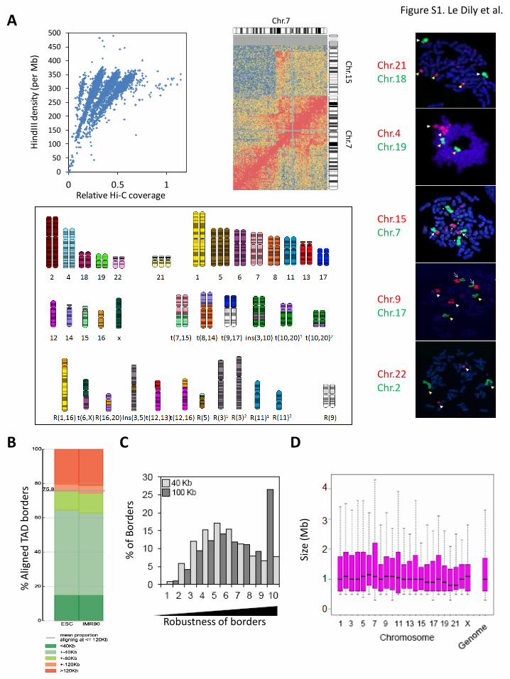
Supplementary Figure 1: T47D genome is organised in TADs.

(A) The linear correlation between number of Hi-C contacts and number of

restriction sites is lost due to changes in copy number allowing determining the

number of copies of each megabase domains present in T47D genome (top left

panel). A snapshot of contact matrix shows an example of translocation

breackpoint between the chromosomes 7 and 15 in T47D cells (top middle

panel). T47D karyotype deduced from the variations in copy number and

translocations events determined as above is represented (bottom panel). Left

panel show examples of 2D-FISH on T47D cells metaphase spreads validating

the karyotype and highlighting changes in ploidy, translocation events as well as

normal chromosomes. (B) Plot showing the correspondence of TADs borders

defined in ESC and IMR90 cells by Dixon et al. and by the approach described

in this study (See Supplementary Methods). (C) Distribution of boundaries

confidence scores for TADs defined at 40 (light grey – n=3027) or 100 Kb (dark

grey – n=2031) resolutions. (D) Distribution of TAD sizes determined at 100 Kb

resolution (N genome=2031).

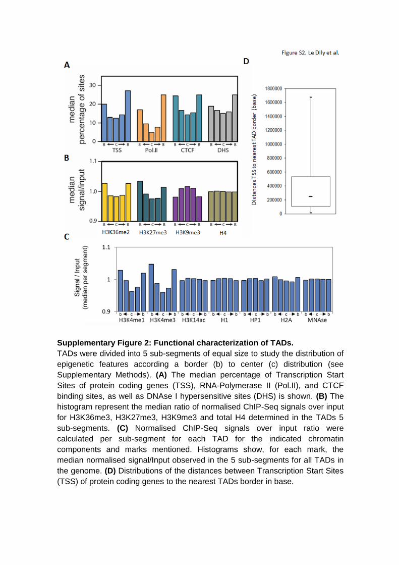
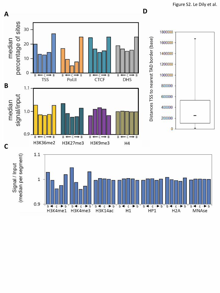
Supplementary Figure 2: Functional characterization of TADs.

TADs were divided into 5 sub-segments of equal size to study the distribution of

epigenetic features according a border (b) to center (c) distribution (see

Supplementary Methods). (A) The median percentage of Transcription Start

Sites of protein coding genes (TSS), RNA-Polymerase II (Pol.II), and CTCF

binding sites, as well as DNAse I hypersensitive sites (DHS) is shown. (B) The

histogram represent the median ratio of normalised ChIP-Seq signals over input

for H3K36me3, H3K27me3, H3K9me3 and total H4 determined in the TADs 5

sub-segments. (C) Normalised ChIP-Seq signals over input ratio were

calculated per sub-segment for each TAD for the indicated chromatin

components and marks mentioned. Histograms show, for each mark, the

median normalised signal/Input observed in the 5 sub-segments for all TADs in

the genome. (D) Distributions of the distances between Transcription Start Sites

(TSS) of protein coding genes to the nearest TADs border in base.

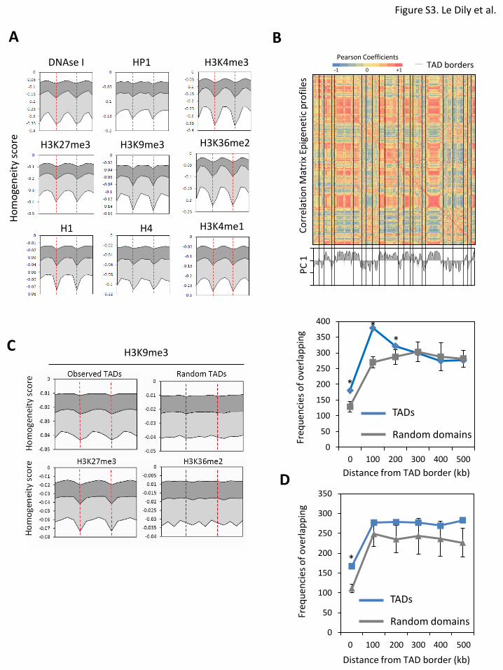
Supplementary Figure 3: TADs are epigenetic domains which chromatin is

coordinately modified upon Pg.

(A) Plots show the homogeneity score of the normalised Chip-Seq signal/Input

ratio between successive sub-segments (see Supplementary Methods) over 3

consecutive TADs for the chromatin marks and components listed. Lines depict

the 25th, 50th and 75th percentiles (from top to bottom respectively) of the scores

computed genome-wide. The red dashed lines correspond to the TADs borders.

(B) Pearson Correlation Coefficient of the combinations of epigenetic marks

were calculated pair-wise in order to generate correlation matrices between

100Kb windows of the genome. Upper panel shows example of such matrices

obtained for the region of chromosome 2 presented in Fig. 2. Location of the

TADs borders are represented by the black dashed lines. These matrices were

submitted to Principal Component Analysis and the first component (PC1) was

used to delimit epigenetic domains. Genome wide, 1812 epigenetic domains

borders were identified and the number of those borders located at increasing

distances from TADs borders or random genomic borders were computed

(Bottom panel). (C) Differences of +Pg/-Pg H3K9me3 Chip-Seq signal between

consecutive sub-segments (see Fig. S3 and Supplementary information) over 3

consecutive TADs in the case of observed (left panel) or randomized (right

panel) TADs borders show that transition between Pg induced changes in

chromatin state occur preferentially at the TAD boundaries. Similar analysis was

performed for other chromatin marks as example H3K27me3 and H3K36me2.

The red dashed lines correspond to the TADs borders. (D) Similar analysis as

described in B was applied using the correlation between the profiles of Pg-

induced changes on chromatin.1695 domains of correlated changes were

identified and their borders and the number of those borders located at

increasing distances from TADs borders or random borders were computed.

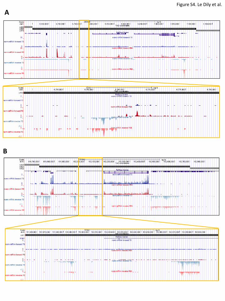
Supplementary Figure 4: TADs respond as unit to the hormone stimulus

(A and B) Genome browser view of RNA-Seq signal within TADs presented in

Figure 2E ((A) U469; (B) U821) highlighting the expression of non-annotated

non-coding transcripts which correlate with the hormone induced changes in

expression observed for the protein coding genes.

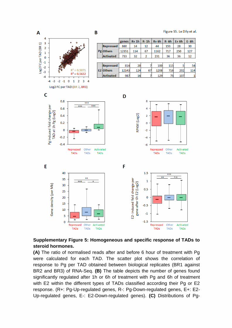
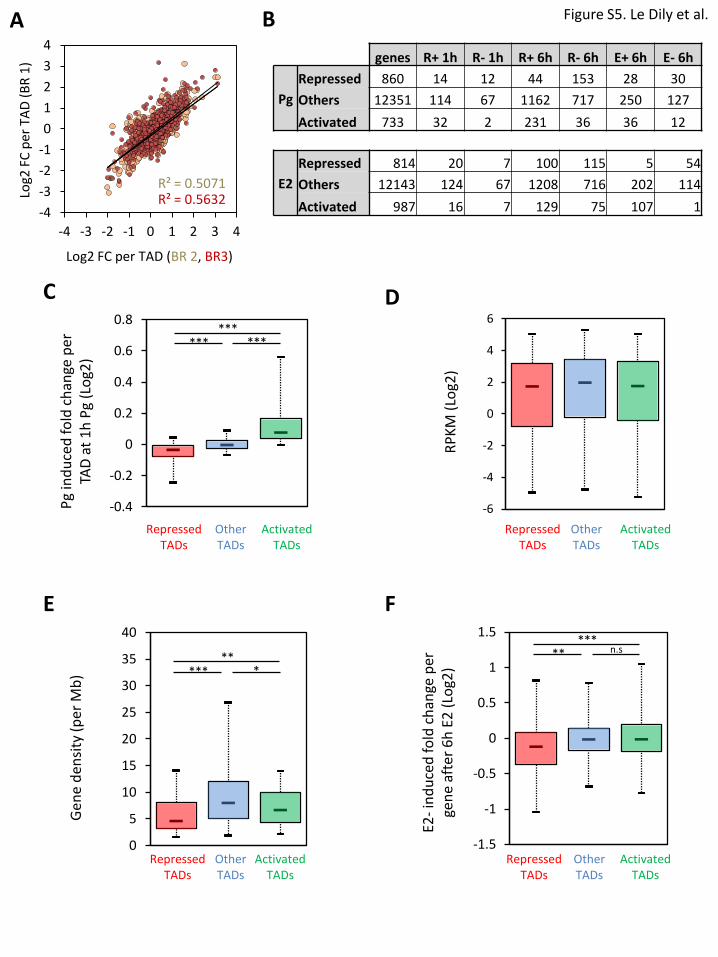
Supplementary Figure 5: Homogeneous and specific response of TADs to

steroid hormones.

(A) The ratio of normalised reads after and before 6 hour of treatment with Pg

were calculated for each TAD. The scatter plot shows the correlation of

response to Pg per TAD obtained between biological replicates (BR1 against

BR2 and BR3) of RNA-Seq. (B) The table depicts the number of genes found

significantly regulated after 1h or 6h of treatment with Pg and 6h of treatment

with E2 within the different types of TADs classified according their Pg or E2

response. (R+: Pg-Up-regulated genes, R-: Pg-Down-regulated genes, E+: E2-

Up-regulated genes, E-: E2-Down-regulated genes). (C) Distributions of Pg-

induced fold changes of expression per TAD after 1h of treatment with Pg

according their type defined at 6h. (D) Boxplots show the basal expression

levels (RPKM – Log2) of genes located within the three types of TADs. (E)

Distributions of the TADs gene densities according the type of TADs. (F)

Distributions of E2-induced fold changes (6h) of expression of genes located in

the different types of Pg responsive TADs. Boxplot whiskers correspond to 5st

and 95th percentiles. (***),(**),(*) indicate P < 0.001, 0.01 and 0.05, respectively

(Bonferroni corrected Mann-Whitney test).

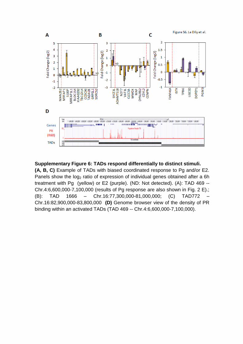
Supplementary Figure 6: TADs respond differentially to distinct stimuli.

(A, B, C) Example of TADs with biased coordinated response to Pg and/or E2.

Panels show the log2 ratio of expression of individual genes obtained after a 6h

treatment with Pg (yellow) or E2 (purple). (ND: Not detected). (A): TAD 469 --

Chr.4:6,600,000-7,100,000 (results of Pg response are also shown in Fig. 2 E).;

(B): TAD 1666 – Chr.16:77,300,000-81,000,000; (C) TAD772 –

Chr.16:82,900,000-83,800,000 (D) Genome browser view of the density of PR

binding within an activated TADs (TAD 469 -- Chr.4:6,600,000-7,100,000).

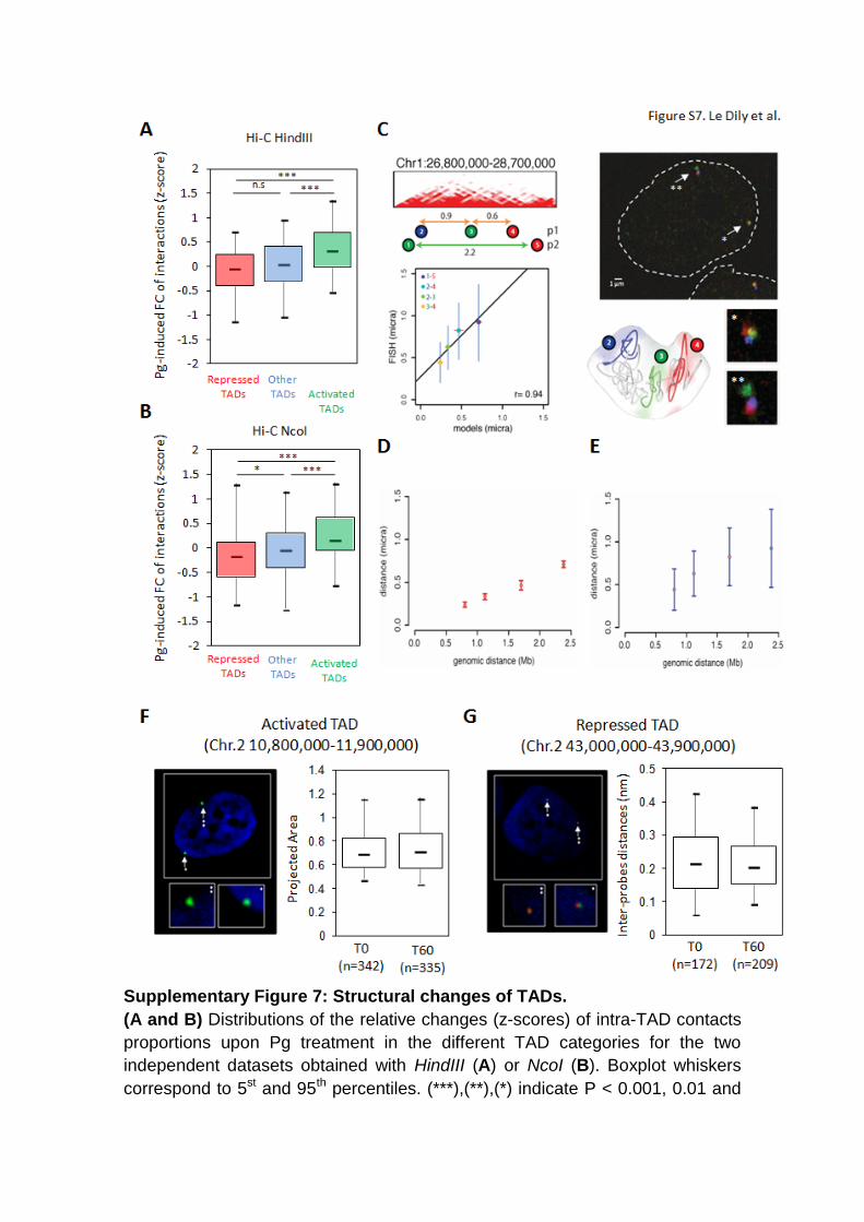
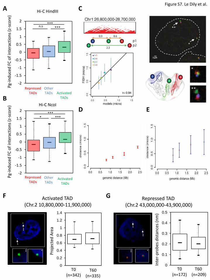
Supplementary Figure 7: Structural changes of TADs.

(A and B) Distributions of the relative changes (z-scores) of intra-TAD contacts

proportions upon Pg treatment in the different TAD categories for the two

independent datasets obtained with HindIII (A) or NcoI (B). Boxplot whiskers

correspond to 5st and 95th percentiles. (***),(**),(*) indicate P < 0.001, 0.01 and

0.05, respectively (Bonferroni corrected Mann-Whitney test). (C) Two pools of

BAC probes located within (p1) or beyond the borders (p2) of a diploid TAD of

Chr.1 were used in 3D-FISH experiments (top right image show a

representative result obtained with the p1; magnifications are shown below).

Virtual 3D-FISH were performed on 3D models of the same region (bottom left

panel). The mean and standard deviation of pair-wise inter-probes 3D distances

obtained in situ (n=60) were compared to the same distances obtained in the

3D models. (D, E) Pair-wise inter-probes 3D distances obtained in the models

(D) or in situ (E) were plotted according the genomic distances that separate

them. (F) FISH experiments using pools of 4 BAC probes covering around 60%

of an activated diploid TADs were performed in T47D cells treated (T60) or not

(T0) with Pg and the area of the projected staining was measured. Boxplots

show the distributions of the projected area obtained at T0 and T60. The

number of individual TADs analyzed for each condition is shown between

brackets. (G) FISH experiments using 2 differently labeled BAC probes in a

repressed diploid TADs were performed in T47D cells treated (T60) or not (T0)

with Pg and the inter-probes distances were measured. Boxplots show the

distribution of the inter-probes distances obtained at T0 and T60. The number of

individual TADs analysed for each condition is shown between brackets.

Chr.7

Ch

r.15

Ch

r.70

50

100

150

200

250

300

350

400

450

500

0 0.5 1

Hin

dII

Iden

sity

(per

Mb

)

Relative Hi-C coverage

Chr.21 Chr.18

Chr.4 Chr.19

Chr.15 Chr.7

Chr.9 Chr.17

Chr.22 Chr.2

A

B C

% A

lign

ed T

AD

bo

rder

s

% o

f B

ord

ers

Robustness of borders

D

Size

(M

b)

Figure S1. Le Dily et al.

A

B

C

D

Dis

tan

ces

TSS

to n

eare

st T

AD

bo

rder

(bas

e)

H3K36me2 H3K27me3 H3K9me3 H4

Figure S2. Le Dily et al.

DNAse I HP1

H1 H4

H3K27me3 H3K9me3 H3K36me2

H3K4me1

H3K4me3

H3K9me3

Ho

mo

gen

eity

sco

re

A

C

-1.00 -0.75 -0.50 -0.25 0.00 0.25 0.50 0.75 1.00

-1 +1 0

Pearson Coefficients

Co

rrel

atio

n M

atri

x Ep

igen

etic

pro

file

s

PC

1

TAD borders

0

50

100

150

200

250

300

350

400

0 100 200 300 400 500

B

D

0

50

100

150

200

250

300

350

Freq

uen

cies

of

ove

rlap

pin

g

0 300 400 500 200 100

Distance from TAD border (kb)

Distance from TAD border (kb)

Freq

uen

cies

of

ove

rlap

pin

g

TADs

Random domains

TADs

Random domains

*

*

*

*

Figure S3. Le Dily et al.

A

B

Figure S4. Le Dily et al.

R² = 0.5071 R² = 0.5632

-4

-3

-2

-1

0

1

2

3

4

-4 -3 -2 -1 0 1 2 3 4

Log2

FC

per

TA

D (

BR

1)

Log2 FC per TAD (BR 2, BR3)

A B

genes R+ 1h R- 1h R+ 6h R- 6h E+ 6h E- 6h

Pg

Repressed 860 14 12 44 153 28 30

Others 12351 114 67 1162 717 250 127

Activated 733 32 2 231 36 36 12

E2

Repressed 814 20 7 100 115 5 54

Others 12143 124 67 1208 716 202 114

Activated 987 16 7 129 75 107 1

C

-0.4

-0.2

0

0.2

0.4

0.6

0.8

D

Pg

ind

uce

d fo

ld c

han

ge p

er

TAD

at

1h

Pg

(Lo

g2)

Repressed TADs

Activated TADs

Other TADs

RP

KM

(Lo

g2)

-6

-4

-2

0

2

4

6

Repressed TADs

Activated TADs

Other TADs

0

5

10

15

20

25

30

35

40

Gen

e d

ensi

ty (p

er M

b)

Repressed TADs

Activated TADs

Other TADs

E

-1.5

-1

-0.5

0

0.5

1

1.5

E2-

ind

uce

d fo

ld c

han

ge p

er

gen

e af

ter

6h

E2

(Lo

g2)

F

Repressed TADs

Activated TADs

Other TADs

*** *** ***

** * ***

*** n.s **

Figure S5. Le Dily et al.

-2

-1

0

1

2

3

4

5

-3

-2

-1

0

1

2

3

-1

-0.5

0

0.5

1

1.5

2

ND

ND

SYC

E1L

AD

AM

TS1

8

ND

T7

VA

T1L

CLE

C3

A

WW

OX

M

AF

DYN

LRB

2

CD

YL2

C

ENP

N

FAM

46

A

IBTK

TPB

G

UB

E3D

DO

PEY

1

PG

M3

MA

N2

B2

M

RFA

P1

S1

00

P

MR

FAP

1L1

B

LOC

1S4

K

IAA

02

32

TB

C1

D1

4

CC

DC

96

TA

DA

2B

G

RP

EL1

SO

RC

S2

A B C

PR (R60)

TADs

D

Genes

Fold

Ch

ange

(lo

g2)

Fold

Ch

ange

(lo

g2)

Fold

Ch

ange

(lo

g2)

Figure S6. Le Dily et al.

D

**

*

*

**

E

C P

g-in

du

ced

FC

of

inte

ract

ion

s (z

-sco

re)

Pg-

ind

uce

d F

C o

f in

tera

ctio

ns

(z-s

core

) A

B

Hi-C HindIII

-2

-1.5

-1

-0.5

0

0.5

1

1.5

2

-2

-1.5

-1

-0.5

0

0.5

1

1.5

2

*** n.s ***

*

Repressed TADs Activated

TADs

Other TADs

Figure S7. Le Dily et al.

0

0.1

0.2

0.3

0.4

0.5

Inte

r-p

rob

es d

ista

nce

s (n

m)

T0 (n=172)

T60 (n=209)

0

0.2

0.4

0.6

0.8

1

1.2

1.4

Pro

ject

ed A

rea

T0 (n=342)

T60 (n=335)

Activated TAD (Chr.2 10,800,000-11,900,000)

Repressed TAD (Chr.2 43,000,000-43,900,000)

*** ***

Repressed TADs

Activated TADs

Other TADs

Hi-C NcoI

F G