dissolved organic matter at the fluvial -marine transition ... · 1 dissolved organic matter at the...

1

Dissolved Organic Matter at the Fluvial-Marine Transition in the

Laptev Sea Using in situ Data and Ocean Color Remote Sensing

Bennet Juhls1, Pier Paul Overduin2, Jens Hölemann3, Martin Hieronymi4, Atsushi Matsuoka5, Birgit

Heim2, Jürgen Fischer1

1Institute for Space Sciences, Department of Earth Sciences, Freie Universität Berlin, Berlin, Germany 5 2Alfred Wegener Institute Helmholtz Centre for Polar and Marine Research, Potsdam, Germany 3Alfred Wegener Institute Helmholtz Centre for Polar and Marine Research, Bremerhaven, Germany 4Institute of Coastal Research, Helmholtz-Zentrum Geesthacht, Geesthacht, Germany 5Takuvik Joint International Laboratory, Département de Biologie, Université Laval, Canada

Correspondence to: Bennet Juhls ([email protected]) 10

Abstract. River water is the main source of dissolved organic carbon (DOC) in the Arctic Ocean. DOC plays an important

role in the Arctic carbon cycle and its export from land to sea is expected to increase as ongoing climate change accelerates

permafrost thaw. However, transport pathways and transformation of DOC in the land-to-ocean transition are mostly

unknown. We collected DOC and aCDOM(λ) samples from 11 expeditions to river, coastal and offshore waters and present a

new DOC-aCDOM(λ) model for the fluvial-marine transition zone in the Laptev Sea The aCDOM(λ) characteristics revealed that 15

the DOM in samples of this dataset are primarily of terrigenous origin. Observed changes in aCDOM and its spectral slopes

indicate that DOM is modified by microbial- and photo-degradation. Ocean Color Remote Sensing (OCRS) provides the

absorption coefficient of colored dissolved organic matter (aCDOM(λ)sat) at λ=440 or 443 nm, which can be used to estimate

DOC concentration at high temporal and spatial resolution over large regions. We tested the statistical performance of five

OCRS algorithms and evaluated the plausibility of the spatial distribution of derived aCDOM(λ)sat. The ONNS algorithm 20

showed the best performance compared to in situ aCDOM(440) (r²=0.72). Additionally, we found ONNS-derived aCDOM(440),

in contrast to other algorithms, to be partly independent of sediment concentration, making ONNS the most suitable

aCDOM(λ)sat algorithm for the Laptev Sea region. The DOC-aCDOM(λ) model was applied to ONNS-derived aCDOM(440) and

retrieved DOC concentration maps showed moderate agreement to in situ data (r²=0.53). The in situ and satellite-retrieved

data were offset by up to several days, which may partly explain the weak correlation for this dynamic region. Satellite-25

derived surface water DOC concentration maps from MERIS satellite data demonstrate rapid removal of DOC within short

time periods in coastal waters of the Laptev Sea, which is likely caused by physical mixing and different types of

degradation processes. Using samples from all occurring water types leads to a more robust DOC-aCDOM(λ) model for the

retrievals of DOC in Arctic shelf and river waters.

30

Biogeosciences Discuss., https://doi.org/10.5194/bg-2019-70Manuscript under review for journal BiogeosciencesDiscussion started: 1 March 2019c© Author(s) 2019. CC BY 4.0 License.

2

1 Introduction

Large volumes of fresh water and dissolved organic matter (DOM) are discharged by Arctic rivers into the Arctic Ocean

(Cooper et al., 2005; Dittmar and Kattner, 2003; Stedmon et al., 2011). Recent studies predict an increase of DOM flux to

the Arctic Ocean with continued climate warming and permafrost thawing (Camill, 2005; Freeman et al., 2001; Frey and

Smith, 2005). This will lead to a cascade of effects on the physical, chemical and biological environment of Arctic shelf 5

waters (Stedmon et al., 2011). These include an increase of radiative heat transfer into surface waters, changes in carbon

sequestration, and reductions of sea-ice extent and thickness (Hill, 2008; Matsuoka et al., 2011).

The Laptev Sea is a wide shelf sea in the eastern Arctic characterized by fresh surface waters from the Lena River,

which delivers around one fifth of all river water to the Arctic Ocean. River water is the main source of DOM and thus of

dissolved organic carbon (DOC) and colored dissolved organic matter (CDOM) to the Laptev Sea shelf (Cauwet and 10

Sidorov, 1996; Gonçalves-Araujo et al., 2015; Kattner et al., 1999; Lobbes et al., 2000; Thibodeau et al., 2014; Vantrepotte

et al., 2015). Moreover, the Lena River has the highest peak concentrations of DOC of all Arctic rivers. The fate and

transformation of DOM as it is discharged to the Arctic Ocean, however, are not well known. Physical and biological

processes, such as photodegradation (Gonçalves-Araujo et al., 2015; Helms et al., 2008, 2014; Opsahl and Benner, 1997) and

microbial degradation (Benner and Kaiser, 2011; Fasching et al., 2015; Fichot and Benner, 2014; Matsuoka et al., 2012, 15

2015), as well as mineralization (Kaiser et al., 2017) and flocculation (Asmala et al., 2014; Guo et al., 2007), are responsible

for the modification and removal of DOM from river-influenced surface waters. Given the strong seasonality of Lena River

runoff (Yang et al., 2002), DOC concentration varies greatly in time and space (Amon et al., 2012; Cauwet and Sidorov,

1996; Raymond et al., 2007; Stedmon et al., 2011). Once exported to the sea, rapid transport of water masses and dislocation

of fronts cause rapid changes in concentrations of surface water constituents at any given location. 20

Therefore, DOC sampling at high temporal and spatial resolutions over long periods is necessary to understand

these changes. Discrete in situ sampling of DOC during expeditions provides point measurements at the time of sampling

and is complicated by the difficulty of accessing shallow water for ocean-going vessels. The resulting inadequacy of sample

coverage in space and time can be overcome by using Ocean Color Remote Sensing (OCRS) data. The absorption coefficient

of CDOM (aCDOM(λ)) at a reference wavelength λ (usually λ=443 nm or λ=440 nm is used) is an optical property of the water 25

and can also be derived with OCRS during ice and cloud-free periods. Hereinafter, we refer to satellite derived aCDOM(λ) as

aCDOM(λ)sat .CDOM absorbs light in the ultraviolet and visible wavelengths (Green and Blough, 1994) and can be used to

estimate DOC concentration. Thus, OCRS provides an alternative to discrete water sampling (Hansell et al., 2002; Matsuoka

et al., 2017). DOC concentration maps with high spatial and temporal resolution will improve our understanding of DOC

dynamics in fluvial-marine transition zones and better quantify carbon cycling. However, most OCRS retrieval algorithms 30

have focused on optically deep (Case 1) waters, which usually correspond to open ocean where all optical water constituents

are coupled to chlorophyll concentration (Kutser et al., 2017; Mobley et al., 2004). Generally, the Laptev Sea coastal to

central-shelf waters and Lena River water can be classified as extreme-absorbing and high-scattering waters with high


3

optical complexity (Case 2) (Heim et al., 2014; Hieronymi et al., 2016). Algorithms for Case 1 water do not provide

reasonable estimates of water constituents in optically complex waters (Antoine et al., 2013). Hieronymi et al. (2017) use a

novel algorithm for the retrieval of OCRS products such as aCDOM(440). This algorithm is specifically designed for a broad

range of concentrations of different water constituents including extremely high absorbing waters with aCDOM(440) of up to

20 m-1. 5

In order to estimate DOC concentration from aCDOM(λ), a number of empirical relationships between in situ DOC

and aCDOM(λ) for Arctic regions are presented in recent studies (Fichot and Benner, 2011; Gonçalves-Araujo et al., 2015;

Mann et al., 2016; Matsuoka et al., 2012; Örek et al., 2013; Spencer et al., 2009; Walker et al., 2013). However, the DOC-

aCDOM(λ) relationship can vary in different water types and can change between seasons and regions (Mannino et al., 2008;

Vantrepotte et al., 2015). Furthermore, existing Arctic datasets of DOC and aCDOM(λ) taken in situ are almost all limited to 10

either offshore, coastal or river waters, so that a DOC-aCDOM(λ) relationship has not been established for the range of water

types in Arctic coastal waters. Samples from near-shore waters from Arctic shelves are under-represented in these datasets.

In order to obtain synoptic DOC concentration maps that cover the fluvial-marine transition, a relationship valid for a

combination of these different water types is required.

Spectral shapes of aCDOM(λ) can provide additional information on the DOM quality and about involved 15

biogeochemical processes that modify the DOM (Carder et al., 1989; Matsuoka et al., 2012; Nelson et al., 2004, 2007).

Various studies use the aCDOM(λ) slope in the UV domain (S275-295) as an indicator of the photodegradation history of the

aCDOM(λ) (Fichot and Benner, 2012; Helms et al., 2008; Del Vecchio and Blough, 2002). Spectral characteristics of aCDOM(λ)

and their correlation to the DOC specific absorption coefficient (a*CDOM(440)) vary across the Eastern Arctic Ocean (EAO)

and the Western Arctic Ocean (WAO) (Stedmon et al., 2011). 20

In this study we aim to better understand the transport of organic material from land to sea in the Arctic and

improve its detection at regional scale in the Laptev Sea, where the Lena River provides a major source of DOM to the

Arctic Ocean. For this, we compile a dataset of DOC and aCDOM(λ) samples collected during multiple expeditions to the

Laptev Sea and Lena River region in order to investigate the optical characteristics and variability of aCDOM(λ). With this

dataset. we develop a new DOC-aCDOM(λ) relationship which we apply to OCRS data in order to estimate DOC concentration 25

from space. We test and evaluate the accuracy of different OCRS algorithms for the fluvial-marine transition zone in the

Laptev Sea.

2 Material and Methods

2.1 Study area & expeditions

The in situ data presented in this study are compiled from several, mostly unpublished datasets from Russian-German 30

expeditions to the Lena River and Laptev Sea that took place from 2010 to 2017 (Table 2). Sampling locations of this dataset


4

include large parts of the western and central Laptev Sea shelf, coastal regions around the Lena River Delta and channels of

the Lena River (Fig. 1).

All ship- and land-based sampling took place during the ice-free period between the end of June and mid-

September. Only one land-based sampling in the central Lena River Delta took place between the end of May and the end of

June, during Lena River peak discharge after the ice break-up. The ship expeditions, which covered offshore shelf waters 5

(NE10, YS11, VB13 and VB14), were conducted on board RV Nikolay Evgenov (NE), RV Jacob Smirnitsky (YS) and RV

Viktor Buynitskiy (VB), respectively. For the other ship expeditions, smaller boats were used for sampling in coastal waters

or on the Lena River. Water sampling at the research station on Samoylov Island (LD14) was carried out from small boats or

from the shore (Fig. 1). Table 1 shows a summary of sampling periods, water types and the sampled parameters of the

individual expedition datasets. 10

2.2 Hydrographic characteristics and sample processing

For each sampling location included in this dataset, vertical profiles of the water column temperature and salinity were

measured with a CTD (Sontek CastAway CTD for LD14, LD15, LD16, Byk17 and a Seabird 19+ for LD10, LD13, NE10,

YS11, VB13, VB14, GA13). In this study we use the practical salinity unit (psu) to describe salinity. Aboard ships and boats,

water samples were taken using Niskin bottles or an UWITEC water sampler at defined depths. Since this study focuses on 15

improving satellite retrievals, only surface water samples (discrete samples from 2 and 5 m water depth) were included in the

compiled dataset. Based on visual examination of the water column characteristics we also included samples from 10 m

depth wherever a thick homogeneous upper mixed layer was present. During the expedition LD14, water samples were taken

from the shore of Samoylov Island at around 0.5 m depth using 5-liter glass bottles

Water samples for DOC analysis were filtered through 0.7µm GF/F filter and acidified with 25 µL HCl suprapur 20

(10 M) after sampling. Samples were stored cool and dark for transport. DOC concentrations were measured using high

temperature catalytic oxidation (TOC-VCPH, Shimadzu). Three measurements of each sample were averaged and after each

10 samples, a blank and a standard (Battle-02, Mauri-09 or Super-05 certified reference material from National Laboratory

for Environmental Testing, Canada) were measured for quality control.

Samples for aCDOM(λ) analysis were filtered through 0.22 µm Millipore GSWP filters (GA13, LD16, Byk17) or 0.7 25

µm Whatman GF/F (LD10, YS11, VB13, VB14, LD14, LD15) after sampling. 100 ml filtrate was stored cool and dark in

amber glass bottles until further analysis. aCDOM(λ) was measured with a spectrophotometer (SPECORD 200, Analytik Jena)

by measuring the absorbance (Aλ) at 1 nm intervals between 200 and 750 nm. Absorption was calculated from the resulting

absorbance measurements via

aCDOM(λ) = 2.303∗𝐴𝜆𝐿

, (1) 30

where L is the path length (length of cuvette), to calculate the aCDOM(λ). Fresh Milli-Q water was used as reference. The

cuvette length varied depending on the expected absorption in the sampled water (1 or 5 cm for river or coastal waters, 5 or

10 cm for offshore shelf waters). Resulting aCDOM(λ) spectra were corrected for baseline offsets by subtracting the mean


5

absorption between 680 and 700 nm, assuming zero absorption at > 680 nm. We focussed on aCDOM at 443 nm since most

OCRS algorithms use this wavelength to retrieve aCDOM(λ). This wavelength corresponds to one spectral band of most

multispectral satellite sensors. Spectral slopes of aCDOM(λ) were calculated by non-linearly fitting the following equation:

aCDOM(λ) = aCDOM(λ0) ∗ 𝑒−𝑆(λ−λ0) , (2)

where aCDOM(λ0) is the absorption coefficient at reference wavelength 0 and S is the spectral slope of aCDOM(λ) for the 5

chosen wavelength range. Spectral slopes of aCDOM(λ) were calculated fitting Eq. (2) for the individual wavelength range.

The DOC specific absorption coefficient at λ=440 nm was calculated with a*CDOM(440)=aCDOM(440)/DOC).

2.3 Satellite data

In order to monitor spatiotemporal variability of DOC in surface waters and test the applicability of the established DOC-

aCDOM(λ) model from this study, we used OCRS. We applied the DOC-aCDOM(λ) model to calculate DOC concentration from 10

satellite-retrieved aCDOM(λ). For this study, we chose the Medium Resolution Imaging Spectrometer (MERIS) because of its

high spectral resolution and spectroradiometric quality. Many OCRS algorithms were developed specifically for this sensor

and are designed for coastal waters. MERIS L1 satellite scenes at reduced resolutions (1 km spatial resolution) were obtained

from the MERIS Catalogue and Inventory (MERCI). We checked all expedition periods for cloud-free MERIS satellites

scenes but only two expeditions from 2010 (LD10 and NE10 ship expeditions) could be used to evaluate the performance of 15

the remote sensing retrieval of the surface water DOC concentration. During those periods, we identified a few scenes with

substantial cloud-free data coverage that were acquired during the 2010 expedition periods. Table 1 lists MERIS scenes used

in this study. In order to visualize satellite-derived results, we generated mosaic images containing the average of the overlap

from multiple satellite scenes to extend the data coverage between cloud gaps. To compare in situ with satellite data, we used

extracted pixel values from each single image. To discuss processes that cause differences between satellite images we 20

extracted reanalysis surface wind data (4 times daily) from the National Centers for Environmental Prediction.

Hieronymi et al. (2017) developed the OLCI (Sentinel-3 Ocean and Land Colour Instrument) Neural Network

Swarm (ONNS) in-water algorithm for the retrieval of OCRS products, among them aCDOM(440). This algorithm is designed

for broad concentration ranges of different water constituents, including extremely high absorbing waters. The algorithm

differentiates 13 optical water types (OWT) and uses specific neural networks (NN) for each OWT. Every NN is trained for 25

narrow concentration ranges. The values of aCDOM(440) used for the training of the NN’s are up 20 m-1. The final product is a

weighted sum of all NNs depending on OWT membership. The standard atmospheric correction of ONNS, namely the

C2RCC (Brockmann et al., 2016), is applied. ONNS makes use of 11 out of the 21 OLCI bands, including the 400 nm band,

which is the only one not delivered by MERIS. In order to retrieve OCRS products with ONNS from MERIS imagery, a

band adaptation NN-algorithm is utilized to extrapolate remote sensing reflectance at 400 nm, which is usually provided with 30

an uncertainty <5 % for these waters (Hieronymi, 2019). Note that the ONNS-algorithm uses the aCDOM(λ) wavelength 440

nm whereas all other algorithms use 443 nm.


6

Additionally, we tested the following open source OCRS algorithms: (1) FUB/WeW MERIS Case-2 Water

properties processor (FUB/WeW) (Schroeder and Schaale, 2005) developed for aCDOM(443) up to 1 m-1), MERIS case 2

water algorithm (C2R) (Doerffer and Schiller, 2007) (aCDOM(443) up to 1 m-1) which is used for the MERIS 3rd

Reprocessing of ESA’s distributed products, and the Case 2 Regional CoastColour (C2RCC) (Brockmann et al., 2016) with

C2RCC (aCDOM(443) up to 1 m-1) and C2X (aCDOM(443) up to 60 m-1). All algorithms used in this study use neural networks 5

trained with databases of radiative transfer simulations or in situ measurements or both to invert the satellite signal into

inherent optical water properties. In this study the atmospheric correction from Case 2 Regional CoastColour processor

(C2RCC) (Brockmann et al., 2016) was used to provide atmosphere corrected reflectances for the OCRS algorithms ONNS,

C2R, C2RCC and C2X. For the FUB/WeW algorithm the atmospheric correction provided by the FUB/WeW processor

(Schroeder and Schaale, 2005) was used. 10

2.3.1 Functions for satellite retrieval evaluation

In order to evaluate the retrieval of a aCDOM(λ)sat from the tested OCRS algorithms, we used a number of evaluation

parameters suggested by Bailey and Werdell, (2006) and Matsuoka et al., (2017). Among them, we use the median of

satellite to in situ ratio (Rt), the semi-interquartile range (SIQR), the median absolute percent error (MPE), and root mean

square error (RMSE). The evaluation parameters are defined as follows: 15

𝑅𝑡 = 𝑚𝑒𝑑𝑖𝑎𝑛( 𝑋𝑠𝑎𝑡

𝑋𝑖𝑛 𝑠𝑖𝑡𝑢), (3)

𝑆𝐼𝑄𝑅 =𝑄3−𝑄1

2, (4)

𝑀𝑃𝐸 = 𝑚𝑒𝑑𝑖𝑎𝑛(100 ∗ |𝑋𝑠𝑎𝑡−𝑋𝑖𝑛 𝑠𝑖𝑡𝑢

𝑋𝑖𝑛 𝑠𝑖𝑡𝑢|), (5)

𝑅𝑀𝑆𝐸 = √∑ [𝑋𝑠𝑎𝑡− 𝑋𝑖𝑛 𝑠𝑖𝑡𝑢]2𝑁

𝑛=1

𝑁, (6)

where Xsat and Xin situ are the satellite-derived and in situ measured aCDOM(443), respectively. Q1 represents the 25th ratio 20

percentile and Q3 represent the 75th ratio percentile.

3 Results

3.1 Spatial and temporal variability of DOC and aCDOM

To examine variability of DOC and CDOM optical properties along the land-ocean continuum of the Lena-Laptev system,

we generated a large dataset that covers spring freshet through late summer from 2010 to 2017 (Table 2). Compared to 25

previously published datasets (Gonçalves-Araujo et al., 2015; Mann et al., 2016; Matsuoka et al., 2012; Walker et al., 2013),

this dataset compiles not only samples of one water type but covers river, coastal and offshore waters throughout the most

variable portion of the open water season.


7

To better understand characteristics of DOC and aCDOM(λ) in freshwater-marine waters, the compiled dataset was

first classified into three water types according to salinity: (1) fresh river water with salinities from 0-0.2, (2) mesohaline

coastal water with salinities from 0.2-16 and (3) offshore waters with salinities >16.

Overall, DOC concentrations tended to decrease from river to offshore. The same trend was also observed in

aCDOM(443). In river water, DOC concentrations and aCDOM(443) ranged from 370 to 1315 µmol L-1 (median=779 µmol L-1) 5

and 1.17 to 7.91 m-1 aCDOM(443) (median=3.61 m-1), respectively (Fig. 2a and b). DOC concentrations and aCDOM(443) in

coastal waters ranged from 205 to 923 µmol L-1 (median=590 µmol L-1) and 0.71 to 3.79 m-1 (median=2.05 m-1),

respectively. Values in offshore water were the least variable of all three water types with DOC concentrations from 91 to

606 µmol L-1 (median=234 µmol L-1) and aCDOM(443) from to 0.077 to 1.86 m-1 (median=0.5 m-1). Generally, observed DOC

and aCDOM(443) values were similar to reported findings from the Lena River and Laptev Sea regions (Amon et al., 2012; 10

Cauwet and Sidorov, 1996; Gonçalves-Araujo et al., 2015; Heim et al., 2014; Raymond et al., 2007; Stedmon et al., 2011).

The spectral UV slope (S275-295) (Fig. 2c) showed similar maximum and median values for river (max.=0.0184

nm-1, median=0.0155 nm-1) and coastal waters (max.=0.0192 nm-1, median=0.0161 nm-1). We observed the lowest S275-295

in the Lena River water during the spring freshet at the beginning of June (LD14, Table 2). Offshore water has significantly

higher S275-295 values ranging from 0.0158 to 0.0267 nm-1 (median=0.195 nm-1). For river and coastal water, S350-500 15

showed a similar variability as S275-295. The range of offshore water S350-500 however, showed substantially higher

variation and covered a broad range (Fig. 2d).

In contrast to trends in DOC concentrations and aCDOM(443), aCDOM(λ) spectral slopes in two distinct spectral

domain (S275-295 and S350-500) tended to increase from river to offshore. While the spectral slopes between river

(max.=0.0184 nm-1, median=0.0155 nm-1) and coastal waters (max.=0.0184 nm-1, median=0.0158 nm-1) were not 20

substantially different, those between the river and offshore were significantly different (p-value=< 10-8).

3.2 CDOM absorption characteristics

We compared salinity and aCDOM(443) for the compiled dataset. As in other river-influenced waters, there was a tight

correlation between aCDOM(443) and salinity, suggesting that physical mixing prevails and plays a role in near-conservative

behavior of aCDOM(λ) (r²=0.87, n=283) (Fig. 3). For this analysis, only coastal and offshore waters were included since river 25

water was constant in salinity but varied seasonally in aCDOM(443) (LD14, Table 2). In the coastal and offshore waters,

aCDOM(443) decreased gradually with increasing salinity. The observed mixing line is similar to the reported mixing-line for

Laptev Sea shelf waters from Heim et al., (2014), which was developed using parts of this compiled dataset (LD10 & YS11).

The reported relationship from Matsuoka et al., (2012), however, shows generally lower aCDOM(443) values in waters of the

WAO along the salinity gradient. S350-500 was very variable along the mixing-line. However, low aCDOM(443) along the 30

mixing line had high S350-500 and higher aCDOM(443) had low S350-500.

Bulk information, combined use of magnitudes and spectral slopes of CDOM absorption are useful for

understanding sources and/or processes involved in the modification of dissolved organic matter (e.g. Fichot and Benner,


8

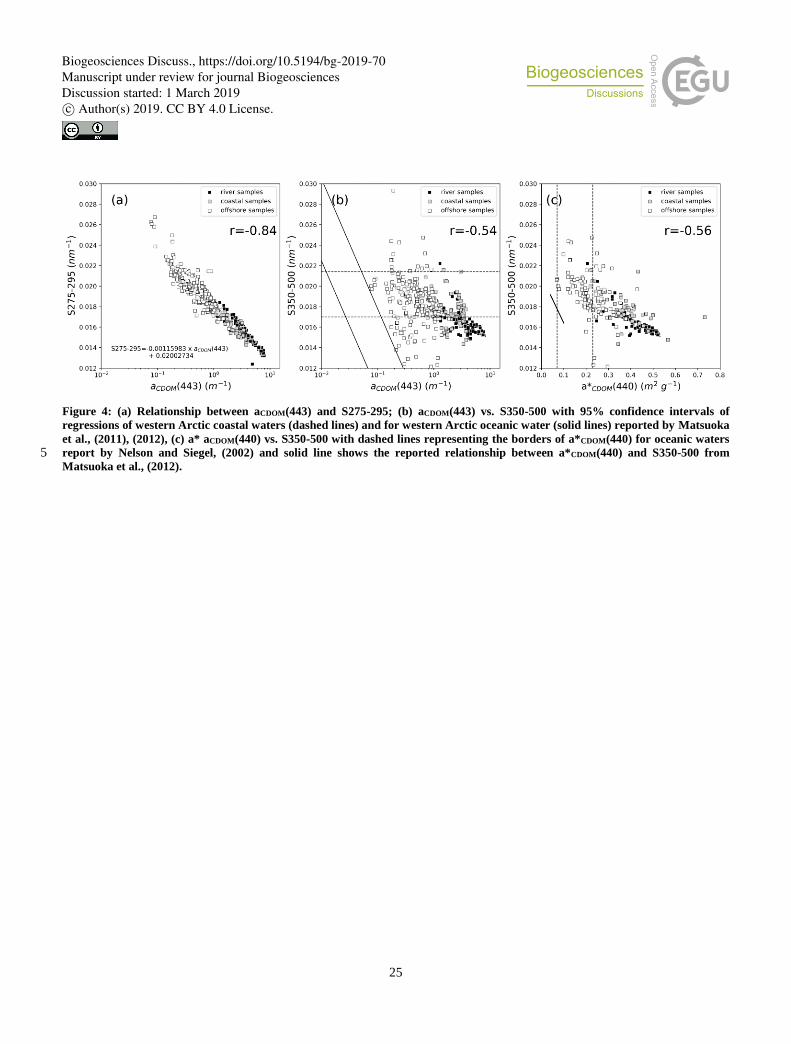
(2012) and Helms et al., (2008). The strongest correlation was observed between aCDOM(443) and the UV slope S275-295

(Fig.4a, r=-0.84). Similar strong correlations were reported by Fichot and Benner, (2011) between aCDOM(350) and S275-295

for coastal waters of the Beaufort Sea in the WAO. Here, we used aCDOM(443) to make the findings useful for the OCRS

community, which usually retrieves aCDOM at 443 nm. The spectral slope S350-500 showed moderate correlation with

aCDOM(443) (Fig.4b, r=-0.54). Furthermore, a high number of S350-500 values were located outside the range of observed 5

S350-500 values for coastal waters of the western Arctic (dashed lines, Fig. 4b).

We observed a moderate correlation between a*CDOM(440) and S350-500 (Fig. 4c, r=-0.56). Most samples from this

study are located below the a*CDOM(440) limits of oceanic water reported by Nelson and Siegel, (2002) indicating that water

samples from this study are primarily river influenced with higher aromaticity. The reported relationship between

a*CDOM(440) and S350-500 from (Matsuoka et al., 2012) deviates strongly in slope of the regression and range of 10

a*CDOM(440) values from this data from the fluvial-marine transition zone of the Laptev Sea.

3.3 DOC – CDOM relationship

Generally, retrieval of optical water properties and water constituents such as DOC from satellite data consists of three steps:

(1) atmospheric correction of the top of atmosphere radiance to the water-leaving or the in-water reflectance, which is

needed as input for the OCRS algorithms, (2) the retrieval of aCDOM(λ)sat from the atmospherically-corrected reflectance 15

received by satellite, and (3) if aCDOM(λ)sat is retrieved from OCRS, DOC can be calculated using an in situ DOC versus in

situ aCDOM(λ) relationship. In the following, we present regional evaluations of a number of OCRS algorithms suitable for

coastal water and an improvement of (3) with a new DOC-aCDOM(λ) relationship from our compiled in situ dataset. The direct

validation and evaluation of different atmospheric corrections (1) is beyond the scope of this study.

We observed a strong relationship between aCDOM(443) and DOC concentration for all water samples including river 20

to marine waters (Fig. 5). One order of magnitude variation in DOC corresponded to more than 2 orders of magnitude of

variation in aCDOM(443) for this sample set, and corresponded to the range from moderately absorbing waters (0.1 – 1.0 m-1)

to highly absorbing waters (>1.0 m-1). After testing different regression models, the best fit was derived with a power

function (Eq. (7), red line in Fig. 5):

𝐷𝑂𝐶 (µ𝑚𝑜𝑙 ∗ 𝐿−1) = 102.525 ∗ 𝑎𝐶𝐷𝑂𝑀(443)0.659 (7) 25

The agreement between model and data (r²=0.96, n=227) allowed estimation of DOC by aCDOM(443) within a 50 % error

range. The highest deviations from the fitted line corresponded to the transition zone between offshore shelf waters and

coastal waters (aCDOM(443)=0.5 – 1.5 m-1) and to the very low end of the aCDOM(443) range (<0.5 m-1). It is noted that the

fitting model of this dataset using only offshore or river water samples would result in a lower slope (exponent=0.617 for

coastal and offshore water, 0.606 for offshore water only) in the resulting DOC-aCDOM(443) model. Including coastal and 30

river samples substantially increased the slope of the fit, which results in higher DOC estimates for high aCDOM(443). The

reported relationship from Mann et al., (2016) is similar for high-aCDOM(443) river water but deviates for low-aCDOM(443)


9

river water and coastal and offshore water. The model presented by Matsuoka et al., (2017) (blue line in Fig. 5) has a lower

slope and results in highest differences for DOC estimation at high aCDOM(443).

Model coefficients for other selected aCDOM(λ) wavelengths are presented in Table A1 (Appendix A). Furthermore,

the relationship between S275-295 and DOC had a slightly weaker correlation with DOC (r²=0.92) than aCDOM(443).

3.4 Satellite retrieved CDOM 5

To estimate the surface water DOC concentration with the presented DOC-aCDOM(λ) model (Eq. (7), Fig. 5) and generate

DOC concentration maps for large scales, we need a robust and accurate retrieval of aCDOM(λ)sat.

We examined the performance of five OCRS algorithm in terms of aCDOM(443)sat retrieval using Eq. (3) to (6). For

this purpose, aCDOM(443)sat retrievals were compared to in situ data from within 10 days of the satellite retrievals. Our

comparisons showed highly varying results (Fig. 6, Fig. B1 (Appendix B), Table 3) and strong under- or overestimation of 10

aCDOM(λ)sat. Particularly in turbulent coastal waters, comparison of aCDOM(443)sat with in situ aCDOM(443) is challenging, given

the fact that the magnitude of CDOM absorption can vary greatly over a short time for the location of a given pixel. ONNS-

derived aCDOM(λ)sat performed best (r²=0.716, Rt= 0.679, SIQR=0.217, %MPE=58.39, RMSE=0.436). The C2X algorithms

performed similarly with a lower r² (0.65) and substantially higher %MPE (100.0) and RMSE (0.919). In addition to the

comparison with in situ data, we evaluated the plausibility of the resulting spatial distributions and observed extremely high 15

C2X-derived aCDOM(443)sat values in the Lena River mouth (up to 10 m-1). Such values of aCDOM(443) were not confirmed by

any reported in situ data. ONNS-derived aCDOM(443)sat showed values which are in the range of in situ observed aCDOM(443).

Other algorithms show clear underestimations of aCDOM(443)sat compared to in situ data (Fig.11, A2). Thus, ONNS was the

only algorithm that produced aCDOM(λ) values in a similar range to in situ measured aCDOM(440).

3.5 Surface water DOC concentrations in coastal waters of the Laptev Sea 20

Using the presented DOC-aCDOM(λ) model, we generated satellite-derived images of surface water DOC concentrations for

the Lena-Laptev Sea region. All scenes were processed with the ONNS algorithm and aCDOM(440) was averaged for each

mosaic. DOC concentrations for two mosaics (Fig. 7b & 7d) were calculated by using the adapted model from Eq. (7) with

coefficients for aCDOM(440) instead of aCDOM(443). The mean time difference between the two mosaics is 31 days. The DOC

mosaic from early August 2010 (Fig. 7b) shows high DOC concentrations over large areas in the eastern Laptev Sea. 25

Concentrations (>600 µmol L-1) were highest in Buor Khaya Bay east of the Lena River Delta where the Lena River exports

most of its water. The plume of the Lena River with high DOC concentrations (~500 µmol L-1) had propagated

northeastward in this scene. The DOC mosaic from September 2010 (Fig. 7d) shows generally lower DOC concentrations

compared to the earlier scene. Highest concentrations were found in the coastal areas in Buor Khaya Bay (east of the Lena

River Delta) and around the Olenek River Delta (west of the Lena River Delta) to the west of the Lena Delta. While ONNS 30

performs well in river-influenced waters, we note that DOC concentrations at the northern edge can be influenced by cloud

masking (patches of high DOC concentrations shown in northeast corner of Fig. 7d).


10

Both quasi-true color satellite images (Fig. 7a & 7c) show sediment-rich, strongly backscattering waters around the

Lena River Delta resulting from fluvial transport. In the satellite image from 07.09.2010 (Fig.7c) there is also a large

strongly backscattering area in the eastern Laptev Sea, where resuspension events in shallow water (5-10 m) occurred

between both acquisition periods (Fig. 1). These resuspension events are not visible in the calculated DOC concentration

maps at right (Fig. 7d). 5

3.5.1 In situ DOC vs. remotely-sensed DOC

To evaluate the satellite-retrieved DOC concentrations, we compared in situ and ONNS-retrieved DOC concentrations using

the presented DOC-aCDOM(λ) model (Fig. 8) and investigated the plausibility of the DOC value ranges and the derived spatial

patterns (Fig. 7b &c). This evaluation revealed a moderate performance (r²=0.53, slope=0.61) (Fig. 8) despite several days

difference in sampling times between satellite and in situ sampling. This comparison constitutes an evaluation and not a 10

direct validation of the method. The latter is hampered by the lack of matching data and the time offsets between satellite

acquisition and in situ sampling dates. The DOC-aCDOM(λ) model presented in this study improved satellite-derived estimates

of DOC concentration compared to estimates using the DOC-aCDOM(λ) relationship reported by Matsuoka 2017 (r²=0.46, Fig.

8).

To spare in situ data for this performance test, data from LD10 was not used to develop the DOC-aCDOM(λ) model 15

(Eq. (7)). The DOC concentrations for NE10 were calculated from in situ aCDOM(443) measurements using Eq. (7), since no

in situ DOC measurements were taken on NE10. These in situ DOC concentrations are therefore not independent, but were

derived from the DOC-aCDOM(443) relationship for the entire dataset. However, samples from NE10 were not used for the

development of the DOC-aCDOM(λ) relationship since in situ DOC was missing. We use the data to test the DOC retrieval for

a wide range of concentrations. Further validation of the DOC retrieval will require additional in situ datasets collected 20

simultaneously with cloud-free, open-water remote sensing acquisitions by using the MERIS successor OLCI.

4 Discussion

4.1 Sources and modification of DOM in the fluvial-marine transition

Our results showed that aCDOM(443) decreases as a function of salinity, indicating that river water is the main source of

CDOM on the Laptev Sea shelf waters and in coastal waters and thus that most CDOM is of terrigenous origin (Fig. 3). 25

Despite the tight relationship, some data points deviated from the mixing line in the salinity range from 2 to 24. Deviations

from the mixing line can result from combined physical, chemical, and biological processes that modify CDOM optical

properties (Asmala et al., 2014; Matsuoka et al., 2015, 2017). Helms et al., (2008) and Matsuoka et al., (2012) suggested that

higher aCDOM(443) and lower S350-500 can be used as a proxy indicating that microbial degradation is more important than

photodegradation. Indeed, we observed higher aCDOM(443) associated with lower S350-500 within a similar salinity range 30

(Fig. 3), pointing towards stronger microbial degradation than photodegradation.


11

Flocculation can also modify CDOM optical properties by removing larger molecules once the river water

encounters saline water. However, given the fact that this process occurs at low salinities (0 to 3; Asmala et al., (2014)),

flocculation alone cannot explain the deviation of aCDOM(443) values apart from the mixing line.

S275-295 was strongly correlated with aCDOM(443) (Fig. 4a), which is mainly associated with the high content lignin

chromophores in our samples (Fichot et al., 2013) and is partly explained by the long exposure of DOM to solar radiation 5

and the resulting photodegradation (Hansen et al., 2016; Helms et al., 2008). Lena River water shows high lignin content and

higher proportion of syringyl and vanyl phenols relative to p-hydrox phenols (Amon et al., 2012). Benner and Kaiser, (2011)

showed that this could make the DOM more subject to photodegradation, which might supports why such a high correlation

was observed.

Compared to the strong relationship between S275-295 and aCDOM(443), a moderate correlation was observed for 10

S350-500 versus aCDOM(443) relationship (Fig. 4b), suggesting different degradation mechanisms were involved during the

transition from river to coastal and offshore waters. Here we use S350-500, which is often used in the OCRS community,

instead of S350-400, which is the wavelength range suggested by Helms et al., (2008). Note that the correlation between

S350-500 and S350-400 is very high (r=0.98) and thus both slopes can be used. The mean river endmember value of S350-

500 at salinity zero was 0.0163 nm-1. This value tends to be lower in the EOA (including Lena river mouth) than in the WAO 15

(Matsuoka et al., 2017; Stedmon et al., 2011). The higher aCDOM(443) associated with the lower spectral slope observed in

our river and coastal waters suggested more aromaticity in waters obtained from Lena-Laptev region (Stedmon et al., 2011).

This was further demonstrated by our higher a*CDOM(443) (Fig. 4c).

The S350-500 versus aCDOM(443) relationship showed a moderate but significant negative correlation and most

samples were within a terrestrial range (dashed lines, Fig.4b). The fact that no samples were within the reported ranges of 20

photodegradation for oceanic waters (solid lines, Fig. 4b) suggest that CDOM in coastal waters of the Laptev Sea would

have been highly influenced by terrestrial inputs but with least photodegradation effect compared to that in oceanic waters

(Matsuoka et al., 2015, 2017). It is likely that high turbidity and thus less transparent water of coastal regions in the Laptev

Sea protects DOM from photodegradation. Data points outside of the ranges might indicate either microbial degradation

and/or sea ice melt (Matsuoka et al., 2017). Given the only minor influence of ice melt waters during most of our field 25

campaigns, microbial degradation is more likely for some of our samples, which is consistent with our explanation for

deviated samples shown in Fig. 3.

The difference in optical properties of aCDOM(λ) observed between EAO and WAO is possibly caused by geological

difference rather than climatic influences (Gordeev et al., 1996). This is partly supported by the chemical characterization of

lignin phenols (Amon et al., 2012). Our results showed specificity of optical properties in the Lena and Laptev Sea and 30

underline the necessity of discussing spectral optical properties when aCDOM(443) and DOC concentration are estimated in

this region.


12

4.2 Linking CDOM absorption to dissolved organic carbon concentration

Previous reported DOC-aCDOM(λ) models such as Walker et al., (2013), Örek et al., (2013) and Mann et al., (2016) for Arctic

rivers, Matsuoka et al., (2012) for WAO and Gonçalves-Araujo et al., (2015) for coastal waters are restricted in their use to

the water type of samples. Our presented DOC-aCDOM(λ) relationship improves reported models from Mann et al., (2016) and

Matsuoka et al., (2017) for the estimation of DOC from aCDOM(443) in DOC-rich waters in transition zones of river and 5

seawater of the Lena-Laptev region. Matsuoka et al. (2017) provided satellite-retrieved DOC concentration maps for coastal

waters of the Lena River Delta region, retrieved with a DOC-aCDOM(443) relationship developed using a pan-Arctic in situ

dataset. However, the retrieved DOC concentrations were likely underestimated compared to in situ measurements in the

coastal regions of the Laptev Sea presented in this study. In coastal or aCDOM(443)-rich, river-influenced water, the difference

between the two relationships is expected to be highest. Applying the Matsuoka et al. (2017) relationship to aCDOM(443)-rich 10

waters outside its validity ranges (>3.3 m-1) would result in underestimation of DOC compared to the relationship presented

in this study. Taking mean Lena River aCDOM(443) of 4.1 m-1, which is similar to the highest aCDOM(443) values in coastal

waters, the difference in modelled DOC concentration between both relationships is 186.8 µmol L-1. The main reason for this

underestimation is likely the lack of near-coastal and river water samples with high DOC for the development of their

relationship. This hypothesis was confirmed by testing the relationship of our dataset by removing coastal and river water. 15

This decreased the slope of the fitting model and lead to an underestimation of DOC in coastal and river waters (without

coastal and river water: slope=0.617). The slope of the reported fitting model from Matsuoka 2017 (0.448) is lower

compared to the fitting model from this study (all samples: slope=0.664). This difference highlights the importance of using

a broad concentration range to develop such relationships.

The broad concentration range of the relationship presented here permits the generation of remotely sensed surface 20

DOC concentration maps of the Laptev Sea across the fluvial-marine transition zone using aCDOM(443). The applicability of

this relationship for other Arctic fluvial-marine transition regions (e.g. Yenisei, Ob, Kolyma, Mackenzie) is untested and the

relationship may need to be extended with regionally specific data.

Previous studies using aCDOM(443) often focused on different wavelengths for aCDOM(λ). The shape of the DOC-

aCDOM(λ) relationship is strongly dependent on the chosen aCDOM(λ) wavelength: whereas DOC- aCDOM(350) shows a linear 25

relationship, aCDOM(443) can be better described with a power function (see Eq. (7)). Table 4 (A1) provides coefficients for

selected aCDOM(λ) wavelengths. We encourage the data publication of all available wavelengths for aCDOM(λ) measurements

in future studies to enable direct comparisons between studies and regions.

4.2.1 ONNS-derived DOC

The evaluation of ONNS-derived aCDOM(λ)sat performed best when tested with in situ data (Table 3). Thus, we selected the 30

ONNS-derived aCDOM(440)sat to calculate DOC concentration based on the Eq. (7). The evaluation of ONNS-derived DOC

concentrations showed moderate performance (r²=0.53). We suggest that the only moderate agreement likely results from


13

rapid movement of near-coastal water fronts. Fluvial-marine transition zones, as in this study area, are characterized by

rapidly moving water fronts with large variations in DOC concentration. A spatial shift of a plume between in situ sampling

and the satellite acquisition can cause large errors in the match-up performance. All samples from LD10 expedition are

located in the near-coastal areas east of the Lena River Delta where rapid movements of water fronts are likely. This could

partly explain deviations comparing in situ measurements and the satellite derived DOC at a given pixel. Taking this into 5

account, the observed agreement shows an adequate retrieval of DOC by satellite using the OCRS algorithm ONNS.

Using satellite-retrieved surface water DOC concentration maps (Fig. 7b & 7d), we demonstrated rapid changes in

DOC concentrations in the Laptev over 1 month in late summer. The rapid DOC decrease can result from a combination of

vertical mixing, dilution, and microbial- and photodegradation of the organic material in the surface water (Fichot et al.,

2013; Holmes et al., 2008; Mann et al., 2012). OCRS could potentially be used to monitor the rapid removal of DOM by 10

degradation from surface waters on Arctic shelves.

4.3 OCRS algorithms in shallow Arctic fluvial-marine transition zones

We observed specific problems of aCDOM(λ)sat retrievals for optically complex shallow shelf waters using different OCRS

algorithms. The retrieved aCDOM(λ)sat in shallow waters often shows a co-variation with high TSM, which is a result of high

particle backscatter in the water such as sediments or some phytoplankton types. In our study, we observed that most OCRS 15

algorithms show a strong coupling of aCDOM(λ)sat and TSM in all areas of high sediment concentration (compare Fig 7 and

11b).

Our study area, the Laptev Sea shelf, is characterized by extremely shallow waters with frequent resuspension of

sediments from the seafloor, for example during storm events. In the Lena River plume, close to the river mouth, where large

amounts of TSM and organic matter are transported to the Arctic Ocean, we expect DOC and TSM to co-vary. Once 20

exported by the Lena River, most particles quickly settle to the seafloor whereas DOM concentration gradually decreases

with increasing physical mixing and ongoing degradation. In offshore resuspension areas with very high TSM concentration,

DOC and TSM do not necessarily co-vary. Large amounts of terrigenous organic matter can be mineralized on short time

scales (about 50 % within a year, Kaiser et al., (2017)) and strongly degraded when deposited in sediments (Bröder et al.,

2016, 2019; Brüchert et al., 2018). 25

We observe a strong increase of TSM concentrations in the eastern Laptev Sea in September (Fig. 9b) compared to

August (Fig. 9a), which is likely caused by differences in wind speed and resulting wave energy leading to resuspension.

During acquisitions in August, wind speeds were very low (NCEP reanalysis mean surface wind speed of 2.06 m/s for 75°N

& 132.5°E from 01.08.2010 – 05.08.2010) whereas in September winds were stronger (NCEP reanalysis mean surface wind

speed of 6.54 m/s for 75°N & 132.5°E from 04.09.2010 – 20.09.2010). A high TSM concentration in the near-coastal 30

regions around the Lena River Delta, caused by the sediment export by the Lena River, is similar in both mosaics.

The evaluation of OCRS algorithms with in situ data showed the generally good performance of the ONNS and the

C2X algorithms (Table 3). However, shallow resuspension areas are not covered by in situ measurements. Thus, the


14

performance of OCRS algorithms cannot be tested in these areas. Whereas the C2X algorithm derives high aCDOM(443) in the

resuspension areas in the eastern Laptev Sea, the ONNS algorithm derives low aCDOM(440) (Fig. 6).

Including all pixels of each scene (Fig. 6), the ONNS-derived aCDOM(440) does not show a linear relationship with

TSM concentration (Fig. 10a). However, using only pixels proximal to the Lena River Delta, we observe a correlation

(r=0.68), which is caused by the covariation of TSM and aCDOM(440) in river plume. The C2X-derived aCDOM(443) shows a 5

linear relationship between aCDOM(443) and TSM (r=0.79). The correlation regimes of the aCDOM(443) and TSM from river

mouth regions and resuspension areas are visible (Fig. 10b). Thus, we show that C2X-derived aCDOM(443) might vary with

TSM. Further confirmation of these satellite-based observations with in situ data is currently not possible due to a lack of in

situ data in shallow areas. A partial independence between ONNS-retrieved aCDOM(440) and TSM is of high importance in

shallow Arctic shelf waters, such as the Laptev Sea. Using C2X algorithm, resuspension events would result in erroneous 10

estimation of aCDOM(443).

Furthermore, the C2X-derived TSM concentration is substantially higher compared to TSM concentration derived

by ONNS (Fig 12b). Örek et al., (2013) and Heim et al., (2014) report TSM concentrations between 10 and 70 mg/L for

Lena River water and up to 18 mg/L in coastal water near the Lena River Delta measured in situ in August 2010. These

values are similar to TSM concentrations derived by the ONNS algorithms but lower than C2X algorithm TSM. Considering 15

overestimation of C2X derived aCDOM(443) and TSM compared to in situ data, the use of neural networks trained for a broad

range of constituent concentration likely leads to inaccurate results. Combination of neural networks with narrow

concentration ranges and a classification into distinct water types (results of classification shown in Fig. C1, Appendix C), as

used in ONNS-algorithm, provide more robust and accurate results in regions with a broad range of water types.

5 Conclusion 20

In this study, we demonstrate sources and modification of dissolved organic matter (DOM) by analysing aCDOM(λ)

characteristics in the fluvial-marine transition zone where the Lena River meets the Laptev Sea. Our results suggest that the

aCDOM(λ) spectral slope S350-500 could be useful to identify and distinguish processes that degrade DOM at this transition.

Comparisons of aCDOM(λ) characteristics from this study with reported values from western Arctic waters identify DOM

sources as primarily terrigenous. 25

We demonstrate the strength of a large in situ dataset that covers multiple water types for deriving the relationship

between the optical DOM properties and DOC concentration in surface water of the Laptev Sea and Lena Delta region. The

broad range of DOC concentrations and aCDOM(443) from river, coastal and offshore water used to develop this model

enables the accurate estimation of DOC by aCDOM(λ) in the transition zone between river and seawater. Comparing satellite-

retrieved aCDOM(440), using the OCRS ONNS algorithm, and in situ aCDOM(440) demonstrates the performance of the 30

algorithm for these optically complex waters. DOC concentrations calculated from satellite data moderately agreed with in

situ DOC measurements (r²=0.53), demonstrating the applicability of the DOC-aCDOM(λ) relationship from our compiled


15

dataset. ONNS-derived aCDOM(440) was found to be independent of the suspended sediment concentration. Thus,

resuspension events and resulting sediment-rich backscattering waters seem to have no or little influence on the accuracy of

ONNS-derived aCDOM(440).

The Arctic coastal waters of the Laptev Sea are a key region for the fate of terrestrial DOM and can be monitored

synoptically using optical remote sensing with a reasonable accuracy. MERIS-retrieved DOC concentrations presented in 5

this study provide a detailed picture of the spatial distribution of the DOC-rich Lena River water on the Laptev Sea shelf and

indicate the rapid changes in the magnitude of DOC concentrations in the surface waters within short time periods. If cloud

distribution allows, optical remote sensing provides data of high spatial and temporal resolution to track freshwater pathways

in the Arctic Ocean, which is of high interest to the oceanographic community.

Data Availability 10

Data has been made available through PANGAEA:

Juhls, Bennet; Hölemann, Jens A; Heim, Birgit; Overduin, Pier Paul; Gonçalves-Araujo, Rafael; Hieronymi, Martin; Fischer,

Jürgen (2019): Surface water Dissolved Organic Matter (DOC, CDOM) in the Laptev Sea and Lena River.

https://doi.pangaea.de/10.1594/PANGAEA.898813

Appendix 15

Appendix A

The regression between DOC and aCDOM(λ) was performed for a number of selected wavelengths (λ) to enable comparisons

with other studies. Table A1 shows regression coefficients dependent on wavelengths.

Appendix B

Performance of all tested OCRS algorithms are shown in Fig. B1. Whereas ONNS and C2X provide reasonable results close 20

to the 1 to 1 line compared to in situ data, other algorithms (C2R, C2RCC, FUB/WeW) underestimate aCDOM(λ)sat strongly.

Appendix C

The percentage membership of each pixel is then used to calculate a weighted sum of different neural networks trained for

different OWTs. Figure C1 shows the OWTs of the processed scenes from Figure 6 & 7. It is visible that Lena River plume

in the coastal waters was classified as OWT 1 (see 1 in Fig. C1) which indicates optically complex, extreme absorbing and 25

high scattering water. The plume between the Lena Delta and the New Siberian Island is characterized by OWT 5 (see 2 in

Fig. C1a & b), which indicated a mixture of high absorbing and scattering waters. The Lena River water plume with

generally case 2, optically complex waters is sharply delineated to the west, where different water types occur (see 3 in Fig.


16

C1 & b). Waters west of this plume were classified as OWT 11 displaying Case 1 waters (generally optically deep waters)

waters with a small fraction of absorbing waters.

Author Contributions

B.J., P.P.O. developed the study design. Field work and data collection for this study was conducted by B.J. in all used years,

by P.P.O. in 2016 and 2017, J.H. in 2010, 2011, 2013 and 2014 and by B.H. in 2010, 2013, 2014, 2015. M.H. processed 5

satellite data with the ONNS algorithm. B.J. compiled and processed all presented data and prepared the manuscript with

editorial contributions from all co-authors.

Competing interests

The authors declare that they have no conflict of interest

Acknowledgements 10

This work was financially supported by Geo.X, the Research Network for Geosciences in Berlin and Potsdam, (grant #

SO_087_GeoX). Transdrift expedition data were obtained within the framework of the Laptev Sea System project, supported

by the German Federal Ministry of Education and Research (BMBF grant # 03G0833) and the Ministry of Education and

Science of the Russian Federation. Part of this study was funded by the Japan Aerospace Exploration Agency (JAXA)

GCOM-C project (Contract #: 16RSTK-007867) to AM. We thank the crews and colleagues on-board the research vessels 15

involved in sampling. We are grateful to the colleagues of the Russian-German Otto-Schmidt-Laboratory in St. Petersburg

for support and accessibility of laboratory instruments for sample analysis. NCEP-Reanalysis data were provided by the

NOAA-CIRES Climate Diagnostics Center, Boulder, CO, USA at http://www. cdc.noaa.gov/. Furthermore, thanks to Antje

Eulenburg for laboratory analysis of several parameter datasets. The Horizon 2020 Nunataryuk project (grant # 773421)

provided support for discussions with a larger group of experts. 20

References

Amon, R. M. W., Rinehart, A. J., Duan, S., Louchouarn, P., Prokushkin, A., Guggenberger, G., Bauch, D., Stedmon, C.,

Raymond, P. A., Holmes, R. M., McClelland, J. W., Peterson, B. J., Walker, S. A. and Zhulidov, A. V.: Dissolved

organic matter sources in large Arctic rivers, Geochim. Cosmochim. Acta, 94, 217–237,

doi:10.1016/J.GCA.2012.07.015, 2012. 25

Antoine, D., Hooker, S. B., Bélanger, S., Matsuoka, A. and Babin, M.: Apparent optical properties of the Canadian Beaufort

Sea &ndash; Part 1: Observational overview and water column relationships, Biogeosciences, 10(7),


17

4493–4509, doi:10.5194/bg-10-4493-2013, 2013.

Asmala, E., Bowers, D. G., Autio, R., Kaartokallio, H. and Thomas, D. N.: Qualitative changes of riverine dissolved organic

matter at low salinities due to flocculation, J. Geophys. Res. Biogeosciences, 119(10), 1919–1933,

doi:10.1002/2014JG002722, 2014.

Bailey, S. W. and Werdell, P. J.: A multi-sensor approach for the on-orbit validation of ocean color satellite data products, , 5

doi:10.1016/j.rse.2006.01.015, 2006.

Benner, R. and Kaiser, K.: Biological and photochemical transformations of amino acids and lignin phenols in riverine

dissolved organic matter, Biogeochemistry, 102(1–3), 209–222, doi:10.1007/s10533-010-9435-4, 2011.

Brockmann, C., Roland, Peters, M., Stelzer, K., Sabine and Ruescas, A.: Evolution of the C2RCC Neural Network for

Sentinel 2 and 3 for the Retrieval of Ocean Color Products in Normal and Extreme Optically Complex Waters, 10

Living Planet Symp., Vol. 740. [online] Available from: http://brockmann.urracreative.com/wp-

content/uploads/2017/11/sco1_12brockmann.pdf (Accessed 1 February 2018), 2016.

Bröder, L., Tesi, T., Salvadó, J. A., Semiletov, I. P., Dudarev, O. V. and Gustafsson, Ö.: Fate of terrigenous organic matter

across the Laptev Sea from the mouth of the Lena River to the deep sea of the Arctic interior, Biogeosciences,

13(17), 5003–5019, doi:10.5194/bg-13-5003-2016, 2016. 15

Bröder, L., Andersson, A., Tesi, T., Semiletov, I. and Gustafsson, Ö.: Quantifying Degradative Loss of Terrigenous Organic

Carbon in Surface Sediments Across the Laptev and East Siberian Sea, Global Biogeochem. Cycles, 33(1), 85–99,

doi:10.1029/2018GB005967, 2019.

Brüchert, V., Bröder, L., Sawicka, J. E., Tesi, T., Joye, S. P., Sun, X., Semiletov, I. P. and Samarkin, V. A.: Carbon

mineralization in Laptev and East Siberian sea shelf and slope sediment, Biogeosciences, 15(2), 471–490, 20

doi:10.5194/bg-15-471-2018, 2018.

Camill, P.: Permafrost Thaw Accelerates in Boreal Peatlands During Late-20th Century Climate Warming, Clim. Change,

68(1–2), 135–152, doi:10.1007/s10584-005-4785-y, 2005.

Carder, K. L., Steward, R. G., Harvey, G. R. and Ortner, P. B.: Marine humic and fulvic acids : Their efEcts on remote

sensing of ocean chlorophyll, Science (80-. )., 34(l), 68–81, 1989. 25

Cauwet, G. and Sidorov, I.: The biogeochemistry of Lena River: organic carbon and nutrients distribution, Mar. Chem.,

53(3–4), 211–227, doi:10.1016/0304-4203(95)00090-9, 1996.

Cooper, L. W., Benner, R., McClelland, J. W., Peterson, B. J., Holmes, R. M., Raymond, P. A., Hansell, D. A., Grebmeier, J.

M. and Codispoti, L. A.: Linkages among runoff, dissolved organic carbon, and the stable oxygen isotope

composition of seawater and other water mass indicators in the Arctic Ocean, J. Geophys. Res. Biogeosciences, 30

110(G2), n/a-n/a, doi:10.1029/2005JG000031, 2005.

Dittmar, T. and Kattner, G.: The biogeochemistry of the river and shelf ecosystem of the Arctic Ocean: a review, Mar.

Chem., 83, 103–120, doi:10.1016/S0304-4203(03)00105-1, 2003.

Doerffer, R. and Schiller, H.: The MERIS Case 2 water algorithm, Int. J. Remote Sens., 28(3–4), 517–535,


18

doi:10.1080/01431160600821127, 2007.

Fasching, C., Behounek, B., Singer, G. A. and Battin, T. J.: Microbial degradation of terrigenous dissolved organic matter

and potential consequences for carbon cycling in brown-water streams, Sci. Rep., 4(1), 4981,

doi:10.1038/srep04981, 2015.

Fichot, C. G. and Benner, R.: A novel method to estimate DOC concentrations from CDOM absorption coefficients in 5

coastal waters, Geophys. Res. Lett., 38(3), doi:10.1029/2010GL046152, 2011.

Fichot, C. G. and Benner, R.: The spectral slope coefficient of chromophoric dissolved organic matter ( S 275-295 ) as a

tracer of terrigenous dissolved organic carbon in river-influenced ocean margins, Limnol. Oceanogr., 57(5), 1453–

1466, doi:10.4319/lo.2012.57.5.1453, 2012.

Fichot, C. G. and Benner, R.: The fate of terrigenous dissolved organic carbon in a river-influenced ocean margin, Global 10

Biogeochem. Cycles, 28(3), 300–318, doi:10.1002/2013GB004670, 2014.

Fichot, C. G., Kaiser, K., Hooker, S. B., Amon, R. M. W., Babin, M., Bélanger, S., Walker, S. A. and Benner, R.: Pan-Arctic

distributions of continental runoff in the Arctic Ocean, Sci. Rep., 3(1), 1053, doi:10.1038/srep01053, 2013.

Freeman, C., Evans, C. D., Monteith, D. T., Reynolds, B. and Fenner, N.: Export of organic carbon from peat soils, Nature,

412(6849), 785–785, doi:10.1038/35090628, 2001. 15

Frey, K. E. and Smith, L. C.: Amplified carbon release from vast West Siberian peatlands by 2100, Geophys. Res. Lett.,

32(9), L09401, doi:10.1029/2004GL022025, 2005.

Gonçalves-Araujo, R., Stedmon, C. A., Heim, B., Dubinenkov, I., Kraberg, A., Moiseev, D. and Bracher, A.: From Fresh to

Marine Waters: Characterization and Fate of Dissolved Organic Matter in the Lena River Delta Region, Siberia,

Front. Mar. Sci., 2, 108, doi:10.3389/fmars.2015.00108, 2015. 20

Gordeev, V. V., Martin, J. M., Sidorov, I. S. and Sidorova, M. V.: A reassessment of the Eurasian river input of water,

sediment, major elements, and nutrients to the Arctic Ocean, Am. J. Sci., 296(6), 664–691,

doi:10.2475/ajs.296.6.664, 1996.

Green, S. A. and Blough, N. V.: Optical absorption and fluorescence properties of chromophoric dissolved organic matter in

natural waters, Limnol. Oceanogr., 39(8), 1903–1916, doi:10.4319/lo.1994.39.8.1903, 1994. 25

Guo, W., Stedmon, C. A., Han, Y., Wu, F., Yu, X. and Hu, M.: The conservative and non-conservative behavior of

chromophoric dissolved organic matter in Chinese estuarine waters, Mar. Chem., 107(3), 357–366,

doi:10.1016/J.MARCHEM.2007.03.006, 2007.

Hansell, D. A., Carlson, C. A. and Amon, R. M. W.: Biogeochemistry of marine dissolved organic matter. [online] Available

from: 30

https://books.google.de/books?hl=de&lr=&id=7iKOAwAAQBAJ&oi=fnd&pg=PP1&dq=Hansell,+D.,+2002.+DO

C+in+the+global+ocean+carbon+cycle.+In:+Hansell,+D.A.,+Craig,+C.A.+(Eds.),+Biogeochemistry+of+Marine+D

issolved+Organic+Matter.+Academic+press,+California.&ots=kx (Accessed 19 February 2019), 2002.

Hansen, A. M., Kraus, T. E. C., Pellerin, B. A., Fleck, J. A., Downing, B. D. and Bergamaschi, B. A.: Optical properties of


19

dissolved organic matter (DOM): Effects of biological and photolytic degradation, Limnol. Oceanogr., 61(3), 1015–

1032, doi:10.1002/lno.10270, 2016.

Heim, B., Abramova, E., Doerffer, R., Günther, F., Hölemann, J., Kraberg, A., Lantuit, H., Loginova, A., Martynov, F.,

Overduin, P. P. and Wegner, C.: Ocean colour remote sensing in the southern Laptev Sea: evaluation and

applications, Biogeosciences, 11(15), 4191–4210, doi:10.5194/bg-11-4191-2014, 2014. 5

Helms, J. R., Stubbins, A., Ritchie, J. D., Minor, E. C., Kieber, D. J. and Mopper, K.: Absorption spectral slopes and slope

ratios as indicators of molecular weight, source, and photobleaching of chromophoric dissolved organic matter,

Limnol. Oceanogr., 53(3), 955–969, doi:10.4319/lo.2008.53.3.0955, 2008.

Helms, J. R., Mao, J., Stubbins, A., Schmidt-Rohr, K., Spencer, R. G. M., Hernes, P. J. and Mopper, K.: Loss of optical and

molecular indicators of terrigenous dissolved organic matter during long-term photobleaching, Aquat. Sci., 76(3), 10

353–373, doi:10.1007/s00027-014-0340-0, 2014.

Hieronymi, M.: Spectral band adaptation of ocean color sensors for applicability of the multi-water biogeo-optical algorithm

ONNS, Opt. Express, submitted, 2019.

Hieronymi, M., Krasemann, H., Müller, D., Brockmann, C., Ruescas, A., Stelzer, K., Bouchra, N., Ruddick, K., Simis, S.,

Tilstone, G., Steinmetz, F. and Regner, P.: Ocean Color Remote Sensing of Extreme Case-2 Waters, spectrum, 2, 4. 15

[online] Available from: https://odnature.naturalsciences.be/downloads/publications/1991hieronymi_withheader.pdf

(Accessed 3 September 2018), 2016.

Hieronymi, M., Müller, D. and Doerffer, R.: The OLCI Neural Network Swarm (ONNS): A Bio-Geo-Optical Algorithm for

Open Ocean and Coastal Waters, Front. Mar. Sci., 4, 140, doi:10.3389/fmars.2017.00140, 2017.

Hill, V. J.: Impacts of chromophoric dissolved organic material on surface ocean heating in the Chukchi Sea, J. Geophys. 20

Res., 113(C7), C07024, doi:10.1029/2007JC004119, 2008.

Holmes, R. M., McClelland, J. W., Raymond, P. A., Frazer, B. B., Peterson, B. J. and Stieglitz, M.: Lability of DOC

transported by Alaskan rivers to the Arctic Ocean, Geophys. Res. Lett., 35(3), L03402,

doi:10.1029/2007GL032837, 2008.

Kaiser, K., Benner, R. and Amon, R. M. W.: The fate of terrigenous dissolved organic carbon on the Eurasian shelves and 25

export to the North Atlantic, J. Geophys. Res. Ocean., 122.1, 4–22, doi:10.1002/2016JC012380, 2017.

Kattner, G., Lobbes, J. ., Fitznar, H. ., Engbrodt, R., Nöthig, E.-M. and Lara, R. .: Tracing dissolved organic substances and

nutrients from the Lena River through Laptev Sea (Arctic), Mar. Chem., 65(1–2), 25–39, doi:10.1016/S0304-

4203(99)00008-0, 1999.

Kutser, T., Koponen, S., Kallio, K. Y., Fincke, T. and Paavel, B.: Bio-optical Modeling of Colored Dissolved Organic 30

Matter, in Bio-optical Modeling and Remote Sensing of Inland Waters, pp. 101–128, Elsevier., 2017.

Lobbes, J. M., Fitznar, H. P. and Kattner, G.: Biogeochemical characteristics of dissolved and particulate organic matter in

Russian rivers entering the Arctic Ocean, Geochim. Cosmochim. Acta, 64(17), 2973–2983, doi:10.1016/S0016-

7037(00)00409-9, 2000.


20

Mann, P. J., Davydova, A., Zimov, N., Spencer, R. G. M., Davydov, S., Bulygina, E., Zimov, S. and Holmes, R. M.:

Controls on the composition and lability of dissolved organic matter in Siberia’s Kolyma River basin, J. Geophys.

Res. Biogeosciences, 117(G1), doi:10.1029/2011JG001798, 2012.

Mann, P. J., Spencer, R. G. M., Hernes, P. J., Six, J., Aiken, G. R., Tank, S. E., McClelland, J. W., Butler, K. D., Dyda, R. Y.

and Holmes, R. M.: Pan-Arctic Trends in Terrestrial Dissolved Organic Matter from Optical Measurements, Front. 5

Earth Sci., 4, 25, doi:10.3389/feart.2016.00025, 2016.

Mannino, A., Russ, M. E. and Hooker, S. B.: Algorithm development and validation for satellite-derived distributions of

DOC and CDOM in the U.S. Middle Atlantic Bight, J. Geophys. Res., 113(C7), C07051,

doi:10.1029/2007JC004493, 2008.

Matsuoka, A., Hill, V., Huot, Y., Babin, M. and Bricaud, A.: Seasonal variability in the light absorption properties of 10

western Arctic waters: Parameterization of the individual components of absorption for ocean color applications, J.

Geophys. Res., 116(C2), C02007, doi:10.1029/2009JC005594, 2011.

Matsuoka, A., Bricaud, A., Benner, R., Para, J., Sempéré, R., Prieur, L., Bélanger, S. and Babin, M.: Tracing the transport of

colored dissolved organic matter in water masses of the Southern Beaufort Sea: relationship with hydrographic

characteristics, Biogeosciences, 9(3), 925–940, doi:10.5194/bg-9-925-2012, 2012. 15

Matsuoka, A., Ortega-Retuerta, E., Bricaud, A. and Babin, M.: Characteristics of colored dissolved organic matter (CDOM)

in the Western Arctic Ocean: Relationships with microbial activities, Deep Sea Res. Part II Top. Stud. Oceanogr.,

118, 44–52, doi:10.1016/J.DSR2.2015.02.012, 2015.

Matsuoka, A., Boss, E., Babin, M., Karp-Boss, L., Hafez, M., Chekalyuk, A., Proctor, C. W., Werdell, P. J. and Bricaud, A.:

Pan-Arctic optical characteristics of colored dissolved organic matter: Tracing dissolved organic carbon in changing 20

Arctic waters using satellite ocean color data, Remote Sens. Environ., 200, 89–101,

doi:10.1016/J.RSE.2017.08.009, 2017.

Mobley, C. D., Stramski, D., Bissett, W. P. and Boss, E.: Optical modeling of ocean waters: is the Case 1-Case 2

classification still useful?, Oceanography, 17, 60–67, doi:10.5670/oceanog.2004.48, 2004.

Nelson, N. B. and Siegel, D. A.: Chromophoric DOM in the Open Ocean, in Biogeochemistry of Marine Dissolved Organic 25

Matter, pp. 547–578, Elsevier., 2002.

Nelson, N. B., Carlson, C. A. and Steinberg, D. K.: Production of chromophoric dissolved organic matter by Sargasso Sea

microbes, , doi:10.1016/j.marchem.2004.02.017, 2004.

Nelson, N. B., Siegel, D. A., Carlson, C. A., Swan, C., Smethie, W. M. and Khatiwala, S.: Hydrography of chromophoric

dissolved organic matter in the North Atlantic, Deep Sea Res. Part I Oceanogr. Res. Pap., 54(5), 710–731, 30

doi:10.1016/J.DSR.2007.02.006, 2007.

Opsahl, S. and Benner, R.: Distribution and cycling of terrigenous dissolved organic matter in the ocean, Nature, 386(6624),

480–482, doi:10.1038/386480a0, 1997.

Örek, H., Doerffer, R., Röttgers, R., Boersma, M. and Wiltshire, K. H.: Contribution to a bio-optical model for remote


21

sensing of Lena River water, Biogeosciences, 10, 7081–7094, doi:10.5194/bg-10-7081-2013, 2013.

Raymond, P. A., McClelland, J. W., Holmes, R. M., Zhulidov, A. V., Mull, K., Peterson, B. J., Striegl, R. G., Aiken, G. R.

and Gurtovaya, T. Y.: Flux and age of dissolved organic carbon exported to the Arctic Ocean: A carbon isotopic

study of the five largest arctic rivers, Global Biogeochem. Cycles, 21(4), n/a-n/a, doi:10.1029/2007GB002934,

2007. 5

Schroeder, T. and Schaale, M.: MERIS Case-2 Water Properties Processor, Version 1.0.1, Institute for Space Sciences, Freie

Universität Berlin (FUB), http://www.brockmann-consult.de/beam/software/plugins/FUB-WeWWater-1.0.1.zip,

2005.

Spencer, R. G. M., Aiken, G. R., Butler, K. D., Dornblaser, M. M., Striegl, R. G., Hernes, P. J., Spencer, R. G. M., Aiken, G.

R., Butler, K. D., Dornblaser, M. M., Striegl, R. G. and Hernes, P. J.: Utilizing chromophoric dissolved organic 10

matter measurements to derive export and reactivity of dissolved organic carbon exported to the Arctic Ocean: A

case study of the Yukon River, Alaska Utilizing chromophoric dissolved organic matter measurements to , Alaska,

Geophys. Res. Lett, 36, doi:10.1029/, 2009.

Stedmon, C. A., Amon, R. M. W., Rinehart, A. J. and Walker, S. A.: The supply and characteristics of colored dissolved

organic matter (CDOM) in the Arctic Ocean: Pan Arctic trends and differences, Mar. Chem., 124(1–4), 108–118, 15

doi:10.1016/J.MARCHEM.2010.12.007, 2011.

Thibodeau, B., Bauch, D., Kassens, H. and Timokhov, L. A.: Interannual variations in river water content and distribution

over the Laptev Sea between 2007 and 2011: The Arctic Dipole connection, Geophys. Res. Lett., 41(20), 7237–

7244, doi:10.1002/2014GL061814, 2014.

Vantrepotte, V., Danhiez, F.-P., Loisel, H., Ouillon, S., Mériaux, X., Cauvin, A. and Dessailly, D.: CDOM-DOC relationship 20

in contrasted coastal waters: implication for DOC retrieval from ocean color remote sensing observation, Opt.

Express, 23(1), 33, doi:10.1364/OE.23.000033, 2015.

Del Vecchio, R. and Blough, N. V: Photobleaching of chromophoric dissolved organic matter in natural waters: kinetics and

modeling, Mar. Chem., 78(4), 231–253, doi:10.1016/S0304-4203(02)00036-1, 2002.

Walker, S. A., Amon, R. M. W. and Stedmon, C. A.: Variations in high-latitude riverine fluorescent dissolved organic 25

matter: A comparison of large Arctic rivers, J. Geophys. Res. Biogeosciences, 118(4), 1689–1702,

doi:10.1002/2013JG002320, 2013.

Yang, D., Kane, D. L., Hinzman, L. D., Zhang, X., Zhang, T. and Ye, H.: Siberian Lena River hydrologic regime and recent

change, J. Geophys. Res. Atmos., 107(D23), ACL 14-1-ACL 14-10, doi:10.1029/2002JD002542, 2002.

30


22

Figures

Figure 1: Map of the Laptev Sea and the Lena River Delta region with sample locations from 11 Russian-German expeditions;

upper left map shows the Arctic Ocean and the location of the Laptev Sea on the Russian Arctic shelf. Bathymetry is shown by 5 black contour lines and water depth in meters.


23

Figure 2: Boxplot of (a) DOC concentration, (b) aCDOM(443), (c) S275-295 and (d) S350-500 for the three water types clustered by

salinity (river <0.2, coastal <16, offshore >16); the red line indicates median of each water type.


24

Figure 3: Relationship between aCDOM(443) and salinity (n=283, r²=0.87) for all available water sampled from less than 10 m water

depth and a salinity >0.2; color of data-points indicates S350-500; red dashed line shows the linear fit representing the mixing line

between Salinity and aCDOM(443) within this dataset. Solid black line shows the reported mixing-line from Heim et al., (2014) and

dashed black line to one from Matsuoka 2012 (adapted to aCDOM(443) using Eq. (2) and a constant slope of 0.018. 5


25

Figure 4: (a) Relationship between aCDOM(443) and S275-295; (b) aCDOM(443) vs. S350-500 with 95% confidence intervals of

regressions of western Arctic coastal waters (dashed lines) and for western Arctic oceanic water (solid lines) reported by Matsuoka

et al., (2011), (2012), (c) a* aCDOM(440) vs. S350-500 with dashed lines representing the borders of a*CDOM(440) for oceanic waters

report by Nelson and Siegel, (2002) and solid line shows the reported relationship between a*CDOM(440) and S350-500 from 5 Matsuoka et al., (2012).


26

Figure 5: Relationship between aCDOM(443) and DOC (r²=0.96). Red line shows the derived model from this dataset. The blue line

shows the relationship from Matsuoka et al. (2017) for a pan-Arctic dataset for offshore and coastal waters. The green line shows

the relationship for Lena River water from Mann et al., (2016). The filled grey area shows the 50% error range. Note that the axes

are displayed in log-scale. 5


27

Figure 6 Surface water aCDOM(λ)sat from MERIS mosaic from 5 scenes from September 2010 (scenes listed in Table 1) for all tested

OCRS algorithms (C2R, ONNS, C2RCC, C2X, FUB/WeW). Squares show in situ aCDOM(443) (aCDOM(440) for ONNS) with colors

according to same color scale as satellite data.


28

Figure 7: (a) Quasi-true color image from 5. August 2010; (b) Surface water ONNS-DOC concentration from satellite mosaics

from 2010-08-03 to 2010-08-05. (c) Quasi-true color image from 7. September 2010. d) Surface water ONNS-DOC concentration

from satellite mosaics from 2010-09-07 and 2010-09-18 to 2010-09-20. Squares in (b) and (d) squares indicate in situ concentrations

with same color scale as satellite data. 5


29

Figure 8: Comparison of in situ DOC and ONNS-derived DOC. The dark gray line shows a linear regression (r²=0.53, slope=0.61,

n=50). The gray area represents the 95 % confidence interval. The red line indicates 1:1 correspondence. Days difference (symbol

color) shows the temporal offset between the satellite scene and in situ water sampling. The dashed black line shows the satellite

DOC concentration calculated by using the DOC-aCDOM(443) relationship from Matsuoka et al., (2017). 5


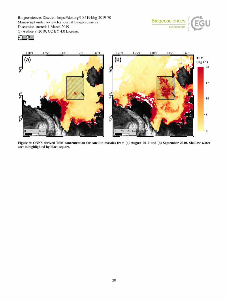
30

Figure 9: ONNS-derived TSM concentration for satellite mosaics from (a) August 2010 and (b) September 2010. Shallow water

area is highlighted by black square.


31

Figure 10 Relationship between (a) ONNS retrieved aCDOM(440) and TSM concentration and (b) C2X retrieved aCDOM(440) and

TSM concentration for the MERIS scene from 07.09.2010. Relationship, using other scenes from September, is not varying

significantly (18.09.2010: ONNS r²=0.22 and C2X r²=0.55, 19.09.2010: ONNS r²=0.23 and C2X r²=0.67, 20.09.2010: ONNS r²=0.03

and C2X r²=0.66) 5


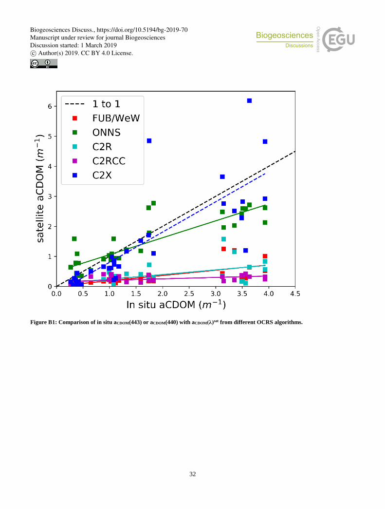
32

Figure B1: Comparison of in situ aCDOM(443) or aCDOM(440) with aCDOM(λ)sat from different OCRS algorithms.


33

Figure C1: Optical water types from ONNS fuzzy logic classification for (a) average of 2010-08-03 to 2010-08-05 and (b) average of

2010-09-07 and 2010-09-18 to 2010-09-20

5


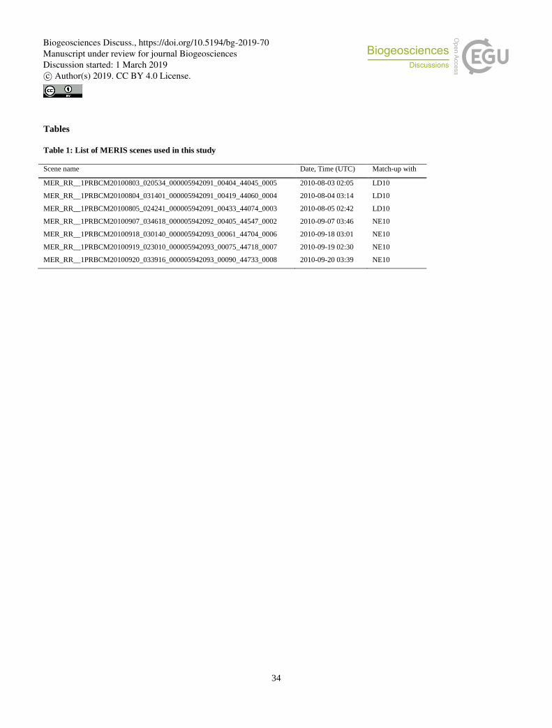
34

Tables

Table 1: List of MERIS scenes used in this study

Scene name Date, Time (UTC) Match-up with

MER_RR__1PRBCM20100803_020534_000005942091_00404_44045_0005 2010-08-03 02:05 LD10

MER_RR__1PRBCM20100804_031401_000005942091_00419_44060_0004 2010-08-04 03:14 LD10

MER_RR__1PRBCM20100805_024241_000005942091_00433_44074_0003 2010-08-05 02:42 LD10

MER_RR__1PRBCM20100907_034618_000005942092_00405_44547_0002 2010-09-07 03:46 NE10

MER_RR__1PRBCM20100918_030140_000005942093_00061_44704_0006 2010-09-18 03:01 NE10

MER_RR__1PRBCM20100919_023010_000005942093_00075_44718_0007 2010-09-19 02:30 NE10

MER_RR__1PRBCM20100920_033916_000005942093_00090_44733_0008 2010-09-20 03:39 NE10


35

Tab

le 2

: E

xp

edit

ion

focu

s re

gio

ns,

yea

rs

an

d r

egio

n.

Mea

n a

nd

sta

nd

ard

dev

iati

on

of

hy

dro

grap

hic

an

d D

OM

para

mete

rs.

Th

e n

um

ber

of

sam

ple

s b

etw

een

DO

C a

nd

aC

DO

M(4

43

) d

iffe

rs f

or

som

e

exp

edit

ion

s a

nd

“n

.a,”

in

dic

ate

s th

at

no D

OC

mea

sure

men

ts w

ere

ma

de.

Exp

edit

ion (

Cod

e)

Focu

s re

gio

n

Yea

r S

easo

n

S (

psu

) D

OC

(µ

mol

L-1

) a C

DO

M(4

43

) (m

-1)

S

275

-295

(nm

-1)

S3

50

-500

(nm

-1)

Len

a 2

010

(L

D1

0)

Coas

tal

2010

Au

g.

6.0

3 ±

6.5

9

563

± 1

56

(n

=29

) 1

3.3

9 ±

0.2

7 (

n=

9)

0.0

152

± 0

.000

6

0.0

167

± 0

.001

9

Tra

nsd

rift

XV

III

(NE

10

) C

entr

al s

hel

f 2

010

Sep

t.

23.6

± 6

.6

n.a

. 0

.66 ±

0.4

6 (

n=

107

) 0

.0196

± 0

.001

6

0.0

175

± 0

.002

8

Tra

nsd

rift

XIX

(Y

S1

1)

Cen

tral

sh

elf

2011

Au

g.

& S

ept.

1

9.6

± 3

.6

239

± 5

5 (

n=

29

) 0

.75 ±

0.2

1 (

n=

26

) 0

.0193

± 0

.000

9

0.0

161

± 0

.012

9

Len

a 2

013

(L

D1

3)

Len

a R

iver

2

013

July

& A

ug.

0.0

1 ±

0.0

5

695

± 7

7 (

n=

28

) 2

3.2

5 ±

0.6

(n

=28

) 0

.016

± 0

.0007

0.0

166

± 0

.000

6

Gon

çalv

es-A

rau

jo e

t al

., (

20

15

)

(GA

13

) C

oas

tal

2013

July

& A

ug.

14.2

± 9

.4

398

± 1

55

(n

=59

) 4

1.5

± 0

.86

(n

=42

) 3

0.0

17

± 0

.0015

0.0

181

± 0

.001

58

Tra

nsd

rift

XX

I (V

B1

3)

Cen

tral

sh

elf

2013

Au

g.

& S

ept.

2

2.6

± 6

.9

n.a

. 0

.71 ±

0.5

5 (

n=

19

) 0

.0201

± 0

.002

3

0.0

184

± 0

.001

7

Len

a 2

014

(L

D1

4)

Len

a R

iver

2

014

May

& J

un

e 0

.01 ±

0.0

5

1049

± 2

48

(n

=5

0)

5.6

6 ±

1.8

5 (

n=

44

) 0

.0145

± 0

.001

0.0

159

± 0

.000

5

Tra

nsd

rift

XX

II (

VB

14

) C

entr

al s

hel

f 2

014

Sep

t.

28.3

± 2

.9

176

± 5

3 (

n=

46

) 0

.36 ±

0.1

9 (

n=

47

) 0

.0208

± 0

.002

1

0.0

196

± 0

.001

64

Len

a 2

015

(L

D1

5)

Len

a R

iver

2

015

July

& S

ept.

0

.01 ±

0.0

5

n.a

. 2

.66 ±

0.7

2 (

n=

12

) 5

0.0

167

± 0

.000

9

0.0

166

± 0

.000

6

Len

a 2

016

(L

D1

6)

Len

a R

iver

&

Coas

tal

2016

Au

g.

& S

ept.

7

.3 ±

9.5

4

99

± 1

64

(n

=17

) 2

.47 ±

1.2

2 (

n=

35

) 0

.0164

± 0

.001

0.0

164

± 0

.001

4

Byk

ovsk

y 2

017

(B

yk

17

) C

oas

tal

2017

Jun

e &

Ju

ly

1.3

± 2

.2

675

± 6

1 (

n=

22

) 2

.6 ±

0.6

9 (

n=

22

) 0

.0161

± 0

.000

9

0.0

19

± 0

.0013

1d

oi.

org

/10

.159

4/P

AN

GA

EA

.842

220

2d

oi.

org

/10

.159

4/P

AN

GA

EA

.844

928

3d

oi.

org

/10

.159

4/P

AN

GA

EA

.875

748

5

4d

oi.

org

/10

.159

4/P

AN

GA

EA

.842

221

5d

oi.

org

/10

.159

4/P

AN

GA

EA

.875

754


36

Table 3: Performance of tested OCRS algorithms for aCDOM(λ)sat with in situ aCDOM(443) or aCDOM(440). Note that not all OCRS

algorithms are developed for the highly absorbing waters (high aCDOM(λ)) found in the Arctic coastal region.

OCRS

algorithm n slope intercept r² Rt SIQR %MPE RMSE

ONNS 34 0.571 0.493 0.716 0.679 0.217 58.39 0.436

C2R 34 0.157 0.087 0.329 3.23 0.075 223.38 0.277

C2RCC 34 0.048 0.157 0.271 3.23 0.093 223.05 0.097

C2X 34 1.023 -0.212 0.652 1.09 0.224 100.0 0.919

FUB/WeW 34 0.178 0.013 0.545 3.76 0.057 276.49 0.2


37

Table A1: Coefficients selected wavelengths for aCDOM(λ) using the equation 𝒃 ∗ 𝐚𝐂𝐃𝐎𝐌(𝛌)𝒄

λ of aCDOM(λ)) b c

254 20.9462548427 0.8483590018983822

350 97.4272121688 0.7260394049434391

375 136.577758485 0.715114349676763

440 322.902097112 0.6667788739998305

443 333.695151626 0.6640204313768572


dissolved organic matter at the fluvial -marine transition ... · 1 dissolved organic matter at the...

Documents