dissipation bounds: recovering from overload - cs.unc.edu · dissipation bounds: recovering from...
TRANSCRIPT
Dissipation Bounds: Recovering from Overload
Jeremy P. Erickson and James H. Anderson
Department of Computer Science, University of North Carolina at Chapel Hill∗
Abstract
The MC2 mixed-criticality framework has been previously proposed for mixing safety-
critical hard real-time (HRT) and mission-critical soft real-time (SRT) software on the same
multicore computer. This paper focuses on the execution of SRT software within this framework.
When determining SRT guarantees, jobs are provisioned based on a provisioned worst-case
execution time (PWCET) that is not very pessimistic and could be overrun. In this paper, we
propose a mechanism to recover from the overload created by such overruns. We propose a
modification to the previously-proposed G-EDF-like (GEL) class of schedulers that uses virtual
time to increase task periods. We then show how to compute dissipation bounds that indicate
how long it takes to return to normal behavior after a transient overload.
1 Introduction
Future cyber-physical systems will require mixing tasks of varying importance. For example, future
unmanned aerial vehicles (UAVs) will require more stringent timing requirements for adjusting flight
surfaces than for long-term decision-making (Herman et al., 2012). The mixed criticality (MC)
framework MC2 has been previously proposed in order to allow these workloads to be simultaneously
supported on a single multicore machine (Herman et al., 2012; Mollison et al., 2010). Using a single
machine allows reductions in size, weight, and power.
In any mixed-criticality system, there are a number of criticality levels. For example, MC2
has four criticality levels, denoted A (highest) through D (lowest). Each MC task is assigned a
∗Work supported by NSF grants CNS 1016954, CNS 1115284, and CNS 1239135; ARO grant W911NF-09-1-0535;and AFRL grant FA8750-11-1-0033.
1
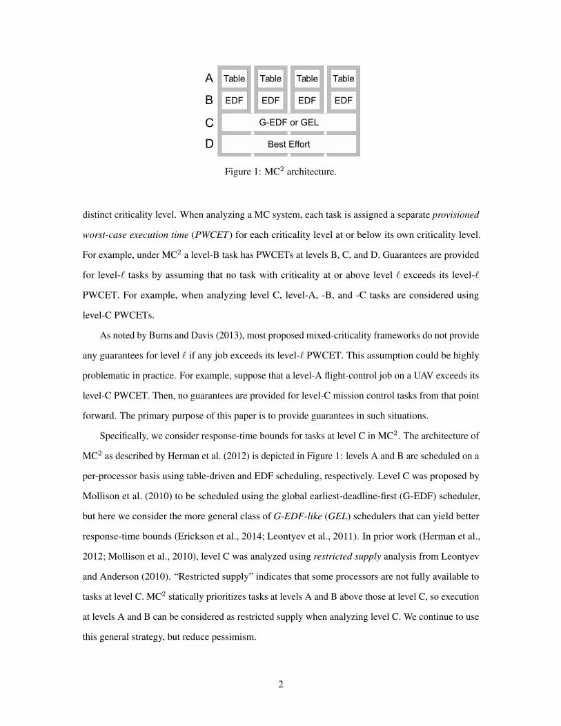
Figure 1: MC2 architecture.
distinct criticality level. When analyzing a MC system, each task is assigned a separate provisioned
worst-case execution time (PWCET) for each criticality level at or below its own criticality level.
For example, under MC2 a level-B task has PWCETs at levels B, C, and D. Guarantees are provided
for level-` tasks by assuming that no task with criticality at or above level ` exceeds its level-`
PWCET. For example, when analyzing level C, level-A, -B, and -C tasks are considered using
level-C PWCETs.
As noted by Burns and Davis (2013), most proposed mixed-criticality frameworks do not provide
any guarantees for level ` if any job exceeds its level-` PWCET. This assumption could be highly
problematic in practice. For example, suppose that a level-A flight-control job on a UAV exceeds its
level-C PWCET. Then, no guarantees are provided for level-C mission control tasks from that point
forward. The primary purpose of this paper is to provide guarantees in such situations.
Specifically, we consider response-time bounds for tasks at level C in MC2. The architecture of
MC2 as described by Herman et al. (2012) is depicted in Figure 1: levels A and B are scheduled on a
per-processor basis using table-driven and EDF scheduling, respectively. Level C was proposed by
Mollison et al. (2010) to be scheduled using the global earliest-deadline-first (G-EDF) scheduler,
but here we consider the more general class of G-EDF-like (GEL) schedulers that can yield better
response-time bounds (Erickson et al., 2014; Leontyev et al., 2011). In prior work (Herman et al.,
2012; Mollison et al., 2010), level C was analyzed using restricted supply analysis from Leontyev
and Anderson (2010). “Restricted supply” indicates that some processors are not fully available to
tasks at level C. MC2 statically prioritizes tasks at levels A and B above those at level C, so execution
at levels A and B can be considered as restricted supply when analyzing level C. We continue to use
this general strategy, but reduce pessimism.
2
Contributions. We provide response-time bounds for MC2 at level C, using arbitrary GEL sched-
ulers. Our analysis is sufficiently general to account for level-A, -B, and -C jobs that overrun their
level-C PWCETs.1 When any job at or above level C overruns its level-C PWCET, the system at
level C may be overloaded. As noted above, this can compromise level-C guarantees. Using the
normal MC2 framework, a task may have its per-job response times permanently increased as a result
of even a single overload event, and multiple overload events could cause such increases to build up
over time. For example, if a system is fully utilized, then there is no “slack” with which to recover
from overload. Therefore, we must alter scheduling decisions to attempt to recover from transient
overload conditions. We do so by scaling task inter-release times and modifying scheduling priorities.
We also provide dissipation bounds on the time required for response-time bounds to settle back to
normal.
Comparison to Related Work. Other techniques for managing overload have been provided in
other settings, although most previously proposed techniques either focus exclusively on uniproces-
sors (Baruah et al., 1991; Beccari et al., 1999; Buttazzo and Stankovic, 1993; Koren and Shasha,
1992; Locke, 1986) or only provide heuristics without theoretical guarantees (Garyali, 2010).
Our paper uses the idea of “virtual time” from Zhang Zhang (1990) (as also used by Stoica
et al. Stoica et al. (1996)), where job separation times are determined using a virtual clock that
changes speeds with respect to the actual clock. In our work, we recover from overload by slowing
down virtual time, effectively reducing the frequency of job releases. Unlike in Stoica et al. (1996),
we never speed up virtual time relative to the normal underloaded system, so we avoid problems that
have previously prevented virtual time from being used on a multiprocessor. To our knowledge, this
work is the first to use virtual time in multiprocessor scheduling.
Some past work on recovering from PWCET overruns in mixed-criticality systems has used
techniques similar to ours, albeit in the context of trying to meet all deadlines (Jan et al., 2013; Santy
et al., 2012, 2013; Su and Zhu, 2013; Su et al., 2013). Our technique is also similar to reweighting
techniques that modify task parameters such as periods. A detailed survey of several such techniques
is provided by Block (2008). Dissipation bounds are a new contribution of our work.
1We note that MC2 supports optional budget enforcement that ensures that tasks at level ` do not exceed their level-`PWCETs. If this technique is used, then it can be guaranteed that no level-C task will overrun its level-C PWCET (thoughlevel-A and -B tasks by definition can overrun their level-C PWCETs). In this paper, we provide analysis for the moregeneral case when budget enforcement is not assumed.
3
Organization. In Section 2, we describe the task model and scheduler, in addition to defining
notation. Then, in Section 3, we show how to compute general response-time bounds. In Section 4,
we leverage the results from Section 3 to show how to compute dissipation bounds, assuming that a
transient overload has completed.
2 System Model
In this paper, we consider a generalized version of GEL scheduling, GEL with virtual time (GEL-v)
scheduling, and a generalized version of the sporadic task model, called the sporadic with virtual
time and overload (SVO) model. We assume that time is continuous.
In our analysis, we consider only the system at level C. In other words, we model level-A and
-B tasks as supply that is unavailable to level C, rather than as explicit tasks. We consider a system
τ = τ0, τ1, . . . , τn−1 of n level-C tasks running on m processors P = P0, P0, . . . , Pm−1. Each
τi is composed of a (potentially infinite) series of jobs τi,0, τi,1, . . .. The release time of τi,k is
denoted as ri,k. We assume that minτi∈τ ri,0 = 0. Each τi,k is prioritized on the basis of a priority
point (PP), denoted yi,k. The time when τi,k actually completes is denoted tci,k. We define the
following quantities that pertain to the execution time of τi,k.
Definition 1. ei,k is the actual execution time of τi,k.
Definition 2. eci,k(t) (completed) is the amount of execution that τi,k completes before time t.
Definition 3. eri,k(t) (remaining) is the amount of execution that τi,k compeletes after time t.
These quantities are related by the following property.
Property 1. For arbitrary τi,k and time t, eci,k(t) + eri,k(t) = ei,k.
We also define what it means for τi,k to be “pending”.
Definition 4. τi,k is defined to be pending at time t if ri,k ≤ t ≤ tci,k.
Under GEL scheduling and the conventional sporadic task model, each task is characterized by a
per-job worst-case execution time (WCET) Ci > 0, a minimum separation Ti > 0 between releases,
and a relative PP Yi ≥ 0. Using the above notation, the system is subject to the following constraints
4
for every τi,k:
ei,k ≤ Ci, (1)
ri,k+1 ≥ ri,k + Ti, (2)
yi,k = ri,k + Yi. (3)
Under the SVO model, we no longer assume a particular WCET (thus allowing overload).
Therefore, (1) is no longer required to hold.
Under GEL-v scheduling and the SVO model, we use a notion of virtual time (as in Stoica et al.
(1996)), and we define the minimum separation time and relative PP of a task with respect to virtual
time after one of its job releases instead of actual time. The purpose of virtual time is depicted in
Figure 2, which we now describe.
In Figure 2, we depict a system that only has level-A and level-C tasks, with one level-A task
per CPU. For level-A tasks, we use the notation (Ti, CCi , C
Ai ), where Ti is task τi’s period, CCi is its
level-C PWCET, and CAi is its level-A PWCET. For level-C tasks, we use the notation (Ti, Yi, Ci),
where all parameters are defined below. Using the analysis provided in this paper, response times
for all jobs can be shown to be bounded in the absence of overload. However, even before the
overload occurs at actual time 12, some jobs complete shortly after their PPs or after successor jobs
are released.
Once an overload occurs, the system can respond by altering virtual time for level C. Virtual
time is based on a global speed function s(t). During normal operation of the system, s(t) is always
1. This means that actual time and virtual time progress at the same rate. However, after an overload
occurs, the scheduler may choose to select 0 < s(t) < 1, at which point virtual time progresses
more slowly than actual time. In Figure 2, the system chooses to use s(t) = 0.5 for t ∈ [19, 29). As
a result, virtual time progresses more slowly in this interval, and new releases of jobs are delayed.
This allows the system to recover from the overload, so at actual time 29, s(t) returns to 1. Observe
that job response times are significantly increased after actual time 12 when the overload occurs, but
after actual time 29, they are similar to before the overload. In fact, the arrival pattern of level A
happens to result in better response times after recovery than before the overload, although this is not
guaranteed under a sporadic release pattern.
5
Figure 2: Example of a system that recovers after an overload.
An actual time t is converted to a virtual time using
v(t) ,∫ t
0s(t) dt. (4)
For example, in Figure 2, v(25) =∫ 25
0 s(t) dt =∫ 19
0 1 dt +∫ 25
19 0.5 dt = 19 + 3 = 22. This
definition leads to the following property:
Property 2. For arbitrary time instants t0 and t1,
v(t1)− v(t0) =
∫ t1
t0
s(t) dt.
Unless otherwise noted, all instants (e.g., t, ri,k, etc.) are specified in actual time, and all
variables except Ti, Yi, and Uvi (all defined below) refer to quantities of actual time.
Under the SVO model, (2) generalizes to
v(ri,k+1) ≥ v(ri,k) + Ti, (5)
and under GEL-v scheduling, (3) generalizes to
v(yi,k) = v(ri,k) + Yi. (6)
For example, in Figure 2, τ1,0 is released at actual time 0, has its PP three units of (both actual and
virtual) time later at actual time 3, and τ1,1 can be released four units of (both actual and virtual) time
6
later at time 4. However, τ1,5 of the same task is released at actual time 21, shortly after the virtual
clock slows down. Therefore, its PP is at actual time 27, which is three units of virtual time after its
release, and the release of τ1,6 can be no sooner than actual time 29, which is four units of virtual
time after the release of τ1,5. However, the execution time of τ1,5 is not affected by the slower virtual
clock.
In light of (5), we denote as bi,k (boundary) the earliest actual time that τi,k+1 could be released,
based on the release time of τi,k. bi,k is indexed using k because it depends on the actual release time
of τi,k, not the actual release time of τi,k+1.
Definition 5. bi,k is the actual time such that v(bi,k) = v(ri,k) + Ti.
Although it is possible to analyze systems where some Yi > Ti, doing so increases proof
complexity without providing any benefit to response-time or dissipation bounds. Therefore, we
assume that for all i,
Yi ≤ Ti. (7)
In our analysis, we will frequently refer to the total work that a task produces from jobs that have
both releases and PPs in a certain interval. We therefore define a function for this quantity.
Definition 6.
Dei (t0, t1) =
∑τi,k∈ω
ei,k
(Demand), where ω is the set of jobs with t0 ≤ ri,k ≤ yi,k ≤ t1.
In order to model processor supply, we use a “service function” as in (Chakraborty et al., 2003;
Leontyev and Anderson, 2010).
Definition 7. βp(t0, t1) is the total number of units of time during which Pp is available to level C
within [t0, t1).
We further characterize processor supply in two parts. First, we assign to each processor Pp
a nominal utilization up, representing how much of its time we expect to be available to level C
in the long term. Within an arbitrary [t0, t1), we expect βp(t0, t1) ≈ up(t1 − t0). For example, in
Figure 2, P0 is available whenever τA1 is not running, so we choose u0 = 1 − 312 = 3
4 , since the
utilization of τA1 at level C is 312 . Similarly, P1 is available whenever τA2 is not running, so we
choose u1 = 1− 16 = 5
6 .
7

Over some intervals [t0, t1], a CPU is available for less time than indicated by nominal utilization
alone. For example, in Figure 2 over [0, 3), P0 is not available at all to level C. Thus, for our second
characterization, we define a supply restriction overload function,
op(t0, t1) , max0, up · (t1 − t0)− βp(t0, t1). (8)
This implies that
βp(t0, t1) ≥ up · (t1 − t0)− op(t0, t1). (9)
For example, consider [0, 3) in Figure 2. By naıvely using nominal utilization, we would expect level
C to receive u0 · (t1 − t0) = 34 · (3 − 0) = 9
4 units of service on P0, but it actually receives 0, so
o0(t0, t1) = 94 . In the absence of overload, there must be some constant σp such that, for all intervals
[t0, t1), op(t0, t1) ≤ upσp, and our model reduces exactly to that used by Leontyev and Anderson
(2010). However, our more general model can be used to account for arbitrary overloads, by allowing
op(t0, t1) > σp when overload occurs within [t0, t1). We also define
utot =∑Pp∈P
up, (10)
which (when supply restriction overload is bounded) represents the total processing capacity available
to the system at level C.
3 Response Time Analysis
In this section, we provide a general method for analyzing response times of a system at level C,
under GEL-v scheduling and with most of the generality of the SVO model. Because we make few
assumptions about overload, this method does not provide response-time bounds that apply to all
jobs. In fact, it applies even in situations where such bounds do not exist. However, we will use
these results, with additional assumptions, in Section 4 to provide dissipation bounds and long-term
response-time bounds in the absence of overload.
Under GEL scheduling applied to ordinary sporadic task systems, Erickson et al. (2014) proved
that tci,k ≤ yi,k + xi + Ci, where xi is a per-task constant. Their proof works by analyzing the
8
behavior of each τi,k after yi,k, because no job with higher priority can be released after yi,k. In the
presence of overload a single per-task xi may not exist. Furthermore, even in cases where such an
xi does exist, it must pessimistically bound all job releases, preventing any analysis of dissipation
bounds. Therefore, we instead define a function of time xi(t) ≥ 0 so that tci,k ≤ yi,k +xi(yi,k) + ei,k.
(We use ei,k in place of Ci because our analysis no longer assumes that ei,k ≤ Ci.) In our analysis, it
is convenient to define xi(t) over all positive real numbers. Furthermore, it will be convenient to
treat xi(t) as merely a safe upper bound. Therefore, we use the following definition.
Definition 8. xi(t) is x-sufficient if xi(t) ≥ 0 and for all τi,k with yi,k ≤ t,
tci,k ≤ t+ xi(t) + ei,k.
Throughout our analysis both here and in Section 4, we will frequently use the following property,
which follows immediately from Definition 8.
Property 3. If c1 ≥ c0 and xi(ta) = c0 is x-sufficient, then xi(ta) = c1 is x-sufficient.
In the remainder of this section, we will provide an x-sufficient value for xi(ta) for each τi and
each time ta (under analysis). We will exhaustively consider the cases depicted in Figure 3 for each
ta, in approximate order by increasing complexity. Note that Cases D and E reference terminology
that will be defined later in this section.
We first consider Case A, which provides the value of xi(ta) when ta < yi,0. This case is trivial.
Theorem 1. If ta < yi,0, then xi(ta) = 0 is x-sufficient.
Proof. This theorem results from the definition of x-sufficient in Definition 8. If ta < yi,0, then the
condition in Definition 8 holds vacuously, because there are no jobs τi,k with yi,k ≤ ta.
We now consider Case B, in which ta = yi,k for some k but tci,k ≤ yi,k + ei,k. This case is
similarly trivial, and we analyze it separately from the cases with ta = yi,k in order to simplify later
proofs.
Theorem 2. If ta = yi,k for some k and tci,k ≤ yi,k + ei,k, then xi(ta) = 0 is x-sufficient.
Proof. This lemma follows immediately from the definition of x-sufficient in Definition 8.
9
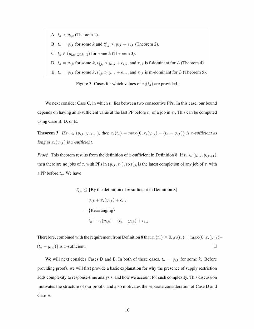
A. ta < yi,0 (Theorem 1).
B. ta = yi,k for some k and tci,k ≤ yi,k + ei,k (Theorem 2).
C. ta ∈ (yi,k, yi,k+1) for some k (Theorem 3).
D. ta = yi,k for some k, tci,k > yi,k + ei,k, and τi,k is f-dominant for L (Theorem 4).
E. ta = yi,k for some k, tci,k > yi,k + ei,k, and τi,k is m-dominant for L (Theorem 5).
Figure 3: Cases for which values of xi(ta) are provided.
We next consider Case C, in which ta lies between two consecutive PPs. In this case, our bound
depends on having an x-sufficient value at the last PP before ta of a job in τi. This can be computed
using Case B, D, or E.
Theorem 3. If ta ∈ (yi,k, yi,k+1), then xi(ta) = max0, xi(yi,k) − (ta − yi,k) is x-sufficient as
long as xi(yi,k) is x-sufficient.
Proof. This theorem results from the definition of x-sufficient in Definition 8. If ta ∈ (yi,k, yi,k+1),
then there are no jobs of τi with PPs in (yi,k, ta), so tci,k is the latest completion of any job of τi with
a PP before ta. We have
tci,k ≤ By the definition of x-sufficient in Definition 8
yi,k + xi(yi,k) + ei,k
= Rearranging
ta + xi(yi,k)− (ta − yi,k) + ei,k.
Therefore, combined with the requirement from Definition 8 that xi(ta) ≥ 0, xi(ta) = max0, xi(yi,k)−
(ta − yi,k) is x-sufficient.
We will next consider Cases D and E. In both of these cases, ta = yi,k for some k. Before
providing proofs, we will first provide a basic explanation for why the presence of supply restriction
adds complexity to response-time analysis, and how we account for such complexity. This discussion
motivates the structure of our proofs, and also motivates the separate consideration of Case D and
Case E.
10
After yi,k, τi,k can be delayed for two reasons: all processors can be occupied by either other
work and/or supply restriction, or some predecessor job of τi,k within τi can be incomplete. We
define work from τj,` as competing with τi,k if yj,` ≤ yi,k and j 6= i, and supply restriction as
competing if it occurs before tci,k. Note that, in order to account for carry-in work, we do not require
that work or supply restriction happen before ri,k in order to say that it is “competing” with τi,k.
We first describe the basic structure of previous analysis from Erickson et al. (2014) in the
absence of supply restriction. Such analysis considers competing work remaining at yi,k. Some
example patterns for the completion of competing work are depicted in Figure 4. Figure 4(a) depicts
the worst-case delay due to competing work rather than a predecessor, when all processors are
occupied until τi,k can begin execution. Figure 4(b) depicts an alternative completion pattern for the
same amount of work. Observe that before tci,k−1, there are idle CPUs. Thus, this example depicts
the situation where τi,k is delayed due to its predecessor.
If some processor is idle, then there must be fewer than m tasks with remaining work. Thus,
in the absence of supply restriction, τi will run continuously until τi,k completes. This is why the
worst-case completion pattern is the one with maximum parallelism, as depicted in Figure 4(a).
For fixed tci,k−1, any other completion pattern might allow τi,k to complete earlier (as happens in
Figure 4(b)) or else does not change the completion time of τi,k (if the delay due to an incomplete
predecessor already dominated). To summarize, in the absence of overload, either the delay due to an
incomplete predecessor dominates, as in Figure 4(b), or the delay due to competing work dominates,
as in Figure 4(a).
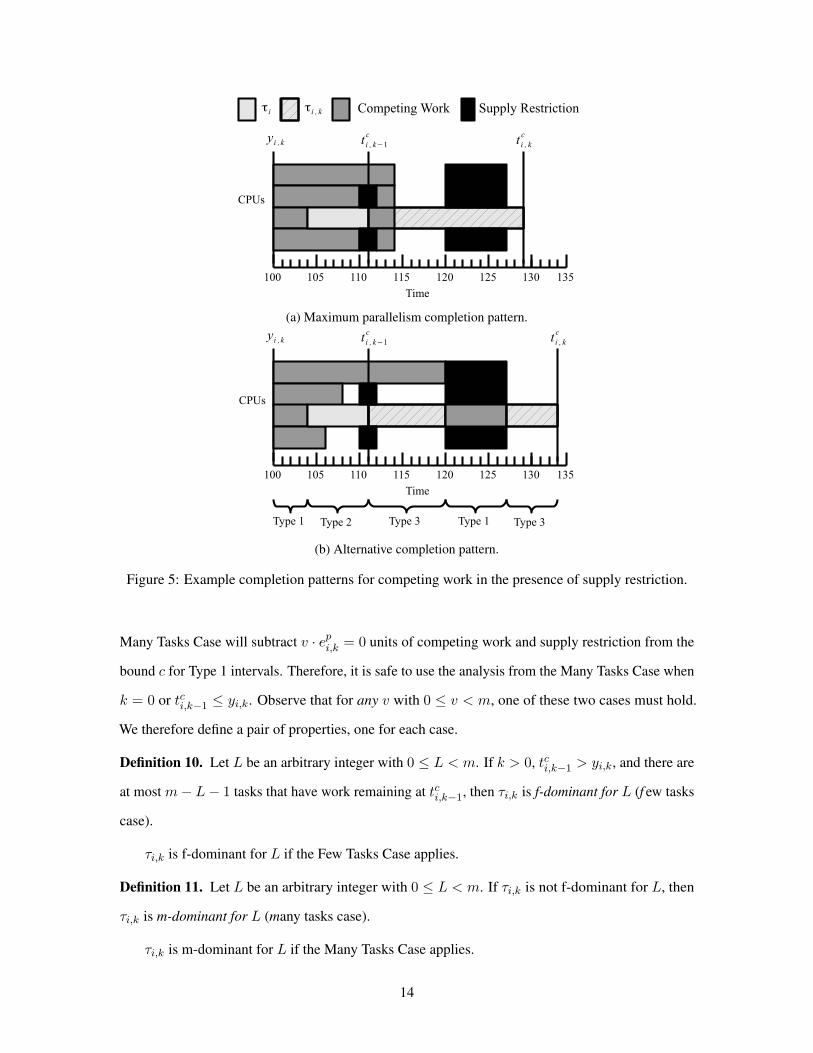
We now consider the effects of introducing supply restriction. Figure 5 depicts similar completion
patterns as Figure 4. As before, τi,k can be delayed either because all processors are occupied by
competing work or supply restriction, or because some predecessor of τi,k within τi is incomplete.
However, as can be seen by comparing Figure 5(a) and Figure 5(b), having all competing work
complete with maximum parallelism is no longer the worst case. This phenomenon occurs because
supply restriction can now prevent the execution of τi even after some processor has become idle,
by reducing the number of available processors below the number of tasks with remaining work.
This increases the complexity of determining the interaction between delays caused by competing
work and delays caused by an incomplete predecessor, as the simple dominance that occurred in the
absence of supply restriction may not occur.
11
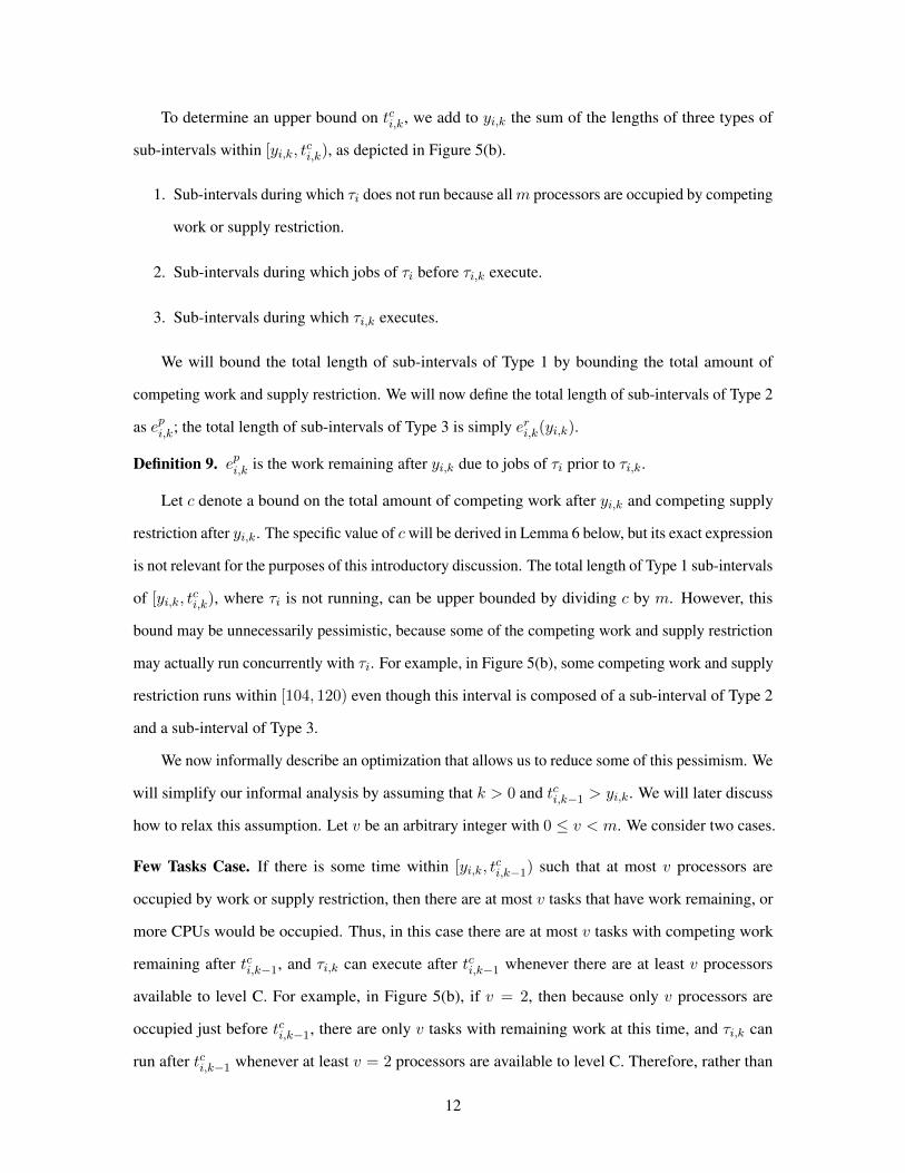
To determine an upper bound on tci,k, we add to yi,k the sum of the lengths of three types of
sub-intervals within [yi,k, tci,k), as depicted in Figure 5(b).
1. Sub-intervals during which τi does not run because allm processors are occupied by competing
work or supply restriction.
2. Sub-intervals during which jobs of τi before τi,k execute.
3. Sub-intervals during which τi,k executes.
We will bound the total length of sub-intervals of Type 1 by bounding the total amount of
competing work and supply restriction. We will now define the total length of sub-intervals of Type 2
as epi,k; the total length of sub-intervals of Type 3 is simply eri,k(yi,k).
Definition 9. epi,k is the work remaining after yi,k due to jobs of τi prior to τi,k.
Let c denote a bound on the total amount of competing work after yi,k and competing supply
restriction after yi,k. The specific value of cwill be derived in Lemma 6 below, but its exact expression
is not relevant for the purposes of this introductory discussion. The total length of Type 1 sub-intervals
of [yi,k, tci,k), where τi is not running, can be upper bounded by dividing c by m. However, this
bound may be unnecessarily pessimistic, because some of the competing work and supply restriction
may actually run concurrently with τi. For example, in Figure 5(b), some competing work and supply
restriction runs within [104, 120) even though this interval is composed of a sub-interval of Type 2
and a sub-interval of Type 3.
We now informally describe an optimization that allows us to reduce some of this pessimism. We
will simplify our informal analysis by assuming that k > 0 and tci,k−1 > yi,k. We will later discuss
how to relax this assumption. Let v be an arbitrary integer with 0 ≤ v < m. We consider two cases.
Few Tasks Case. If there is some time within [yi,k, tci,k−1) such that at most v processors are
occupied by work or supply restriction, then there are at most v tasks that have work remaining, or
more CPUs would be occupied. Thus, in this case there are at most v tasks with competing work
remaining after tci,k−1, and τi,k can execute after tci,k−1 whenever there are at least v processors
available to level C. For example, in Figure 5(b), if v = 2, then because only v processors are
occupied just before tci,k−1, there are only v tasks with remaining work at this time, and τi,k can
run after tci,k−1 whenever at least v = 2 processors are available to level C. Therefore, rather than
12
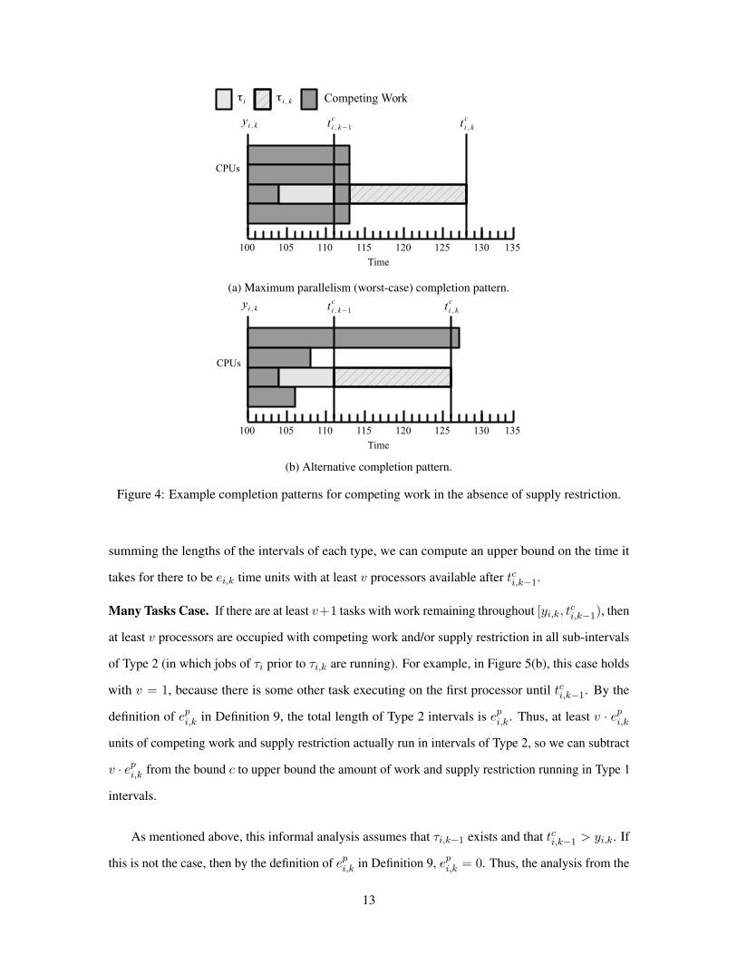
(a) Maximum parallelism (worst-case) completion pattern.
(b) Alternative completion pattern.
Figure 4: Example completion patterns for competing work in the absence of supply restriction.
summing the lengths of the intervals of each type, we can compute an upper bound on the time it
takes for there to be ei,k time units with at least v processors available after tci,k−1.
Many Tasks Case. If there are at least v+1 tasks with work remaining throughout [yi,k, tci,k−1), then
at least v processors are occupied with competing work and/or supply restriction in all sub-intervals
of Type 2 (in which jobs of τi prior to τi,k are running). For example, in Figure 5(b), this case holds
with v = 1, because there is some other task executing on the first processor until tci,k−1. By the
definition of epi,k in Definition 9, the total length of Type 2 intervals is epi,k. Thus, at least v · epi,kunits of competing work and supply restriction actually run in intervals of Type 2, so we can subtract
v · epi,k from the bound c to upper bound the amount of work and supply restriction running in Type 1
intervals.
As mentioned above, this informal analysis assumes that τi,k−1 exists and that tci,k−1 > yi,k. If
this is not the case, then by the definition of epi,k in Definition 9, epi,k = 0. Thus, the analysis from the
13
(a) Maximum parallelism completion pattern.
(b) Alternative completion pattern.
Figure 5: Example completion patterns for competing work in the presence of supply restriction.
Many Tasks Case will subtract v · epi,k = 0 units of competing work and supply restriction from the
bound c for Type 1 intervals. Therefore, it is safe to use the analysis from the Many Tasks Case when
k = 0 or tci,k−1 ≤ yi,k. Observe that for any v with 0 ≤ v < m, one of these two cases must hold.
We therefore define a pair of properties, one for each case.
Definition 10. Let L be an arbitrary integer with 0 ≤ L < m. If k > 0, tci,k−1 > yi,k, and there are
at most m− L− 1 tasks that have work remaining at tci,k−1, then τi,k is f-dominant for L (f ew tasks
case).
τi,k is f-dominant for L if the Few Tasks Case applies.
Definition 11. Let L be an arbitrary integer with 0 ≤ L < m. If τi,k is not f-dominant for L, then
τi,k is m-dominant for L (many tasks case).
τi,k is m-dominant for L if the Many Tasks Case applies.
14
In Section 3.1 below, we will consider Case D, in which τi,k is f-dominant for L. Then, in
Section 3.2, we will consider Case E, in which τi,k is m-dominant for L.
3.1 Case D: ta = yi,k for some k and τi,k is f-dominant for L.
In this case, we use the Few Tasks Case with v = m − L − 1. Recall from the above discussion
that in this case, τi,k runs after tci,k−1 whenever there are at least v processors available to level C.
Lemma 2 below provides a bound on tci,k in this case. Lemma 1 is used to prove Lemma 2.
Lemma 1. For any integer 0 ≤ v ≤ m, in any time interval [t0, t1) there are at least
(t1 − t0)−∑Pp∈ζ
((1− up) · (t1 − t0) + op(t0, t1))
units of time during which at least v processors are available to level C, where ζ is the set of v
processors that minimizes the sum.
Proof. We prove this lemma by induction. Without loss of generality, we fix t0 and t1 and assume
that P is ordered by increasing (1− up)(t1 − t0) + op(t0, t1). We prove the stronger condition that
within [t0, t1), there are (t1 − t0)−∑v
p=1((1− up(t1 − t0) + op(t0, t1)) units time during which
processors P1 through Pv are available to level C.
As the base case, we consider v = 0. During any time instant, it is vacuously true that all
processors in the empty set are available to level C, so there are t1 − t0 such units of time in [t0, t1)
and the lemma holds.
For the inductive case, assume that there are
(t1 − t0)−v∑p=1
((1− up) · (t1 − t0) + op(t0, t1)) (11)
units of time in [t0, t1) during which processors P1 through Pv are available to level C.
By the definition of βv+1(t0, t1) in Definition 7, Pv+1 is unavailable to level C in [t0, t1) for
(t1 − t0)− βv+1(t0, t1)
≤ By (9)
15
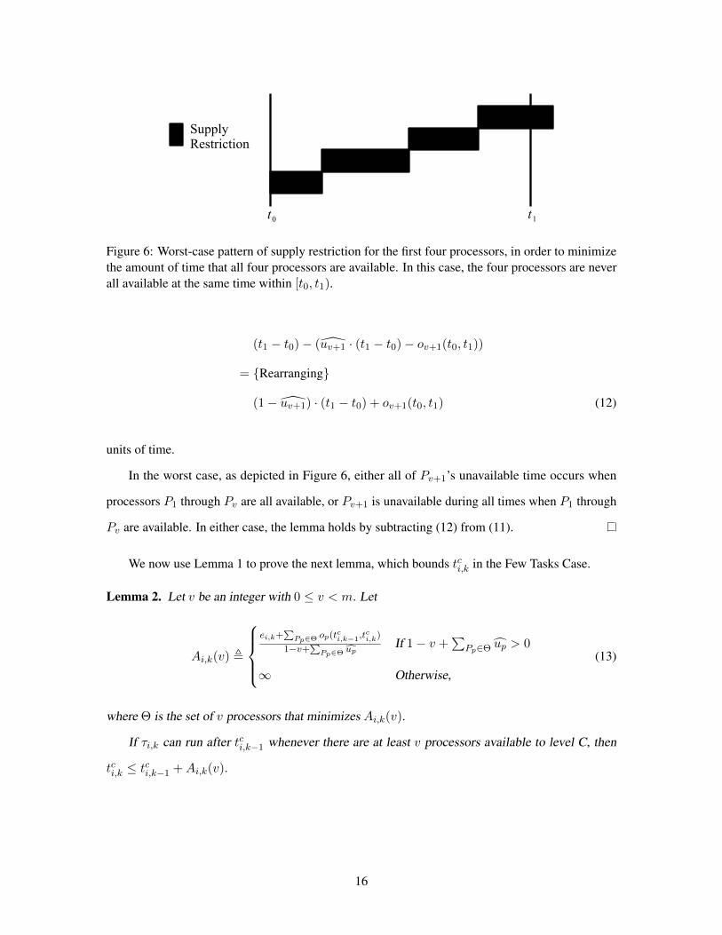
Figure 6: Worst-case pattern of supply restriction for the first four processors, in order to minimizethe amount of time that all four processors are available. In this case, the four processors are neverall available at the same time within [t0, t1).
(t1 − t0)− (uv+1 · (t1 − t0)− ov+1(t0, t1))
= Rearranging
(1− uv+1) · (t1 − t0) + ov+1(t0, t1) (12)
units of time.
In the worst case, as depicted in Figure 6, either all of Pv+1’s unavailable time occurs when
processors P1 through Pv are all available, or Pv+1 is unavailable during all times when P1 through
Pv are available. In either case, the lemma holds by subtracting (12) from (11).
We now use Lemma 1 to prove the next lemma, which bounds tci,k in the Few Tasks Case.
Lemma 2. Let v be an integer with 0 ≤ v < m. Let
Ai,k(v) ,
ei,k+
∑Pp∈Θ op(tci,k−1,t
ci,k)
1−v+∑Pp∈Θ up
If 1− v +∑
Pp∈Θ up > 0
∞ Otherwise,(13)
where Θ is the set of v processors that minimizes Ai,k(v).
If τi,k can run after tci,k−1 whenever there are at least v processors available to level C, then
tci,k ≤ tci,k−1 +Ai,k(v).
16
Proof. If Ai,k(v) is infinite, then the lemma must hold by our assumption that the available supply
is eventually infinite, and thus τi,k eventually completes. Thus, we assume that Ai,k(v) is finite.
Therefore, 1− v +∑
Pp∈Θ up > 0.
We use proof by contradiction. Suppose tci,k > tci,k−1 +Ai,k(v). Then, by Lemma 1, the number
of time units in [tci,k−1, tci,k) with v processors available to level C is at least
(tci,k − tci,k−1)−∑Pp∈ζ
((1− up)(tci,k − tci,k−1) + op(tci,k−1, t
ci,k))
≥ By the definition of ζ in Lemma 1, because Θ has v processors
(tci,k − tci,k−1)−∑Pp∈Θ
((1− up)(tci,k − tci,k−1) + op(tci,k−1, t
ci,k))
= Rearranging1− v +∑Pp∈Θ
up
(tci,k − tci,k−1)−∑Pp∈Θ
op(tci,k−1, t
ci,k)
> Because tci,k > tci,k−1 +Ai,k(v) and 1− v +∑
Pp∈Θ up > 01− v +∑Pp∈Θ
up
Ai,k(v)−∑Pp∈Θ
op(tci,k−1, t
ci,k)
= By (13), because Ai,k(v) is finite1− v +∑Pp∈Θ
up
· ei,k +∑
Pp∈Θ op(tci,k−1, t
ci,k)
1− q +∑
Pp∈Θ up−∑Pp∈Θ
op(tci,k−1, t
ci,k)
= Rearranging
ei,k. (14)
However, because τi,k can run after tci,k−1 whenever there are at least v processors available to level
C, τi,k must have executed for longer than ei,k units. This is a contradiction.
We now use this result to provide a bound on xi(ta) to handle Case D.
Theorem 4. If ta = yi,k for some k and τi,k is f-dominant for L, then xi(ta) = xfi,k is x-sufficient,
where
xfi,k , tci,k−1 − yi,k +Ai,k(m− L− 1)− ei,k (15)
17
( few tasks).
Proof. By the definition of f-dominant for L in Definition 10, because no new competing work is
released after yi,k, throughout (tci,k−1, tci,k], there are at most m− L− 1 tasks that have remaining
competing work. Therefore, whenever at least m− L− 1 processors are available to level C within
(tci,k−1, tci,k], τi,k is running. Thus,
tci,k ≤ By Lemma 2
tci,k−1 +Ai,k(m− L− 1)
= Rearranging
yi,k + (tci,k−1 − yi,k +Ai,k(m− L− 1)− ei,k) + ei,k
= By the definition of xfi,k in (15)
yi,k + xfi,k + ei,k.
Thus, by the definition of x-sufficient in Definition 8, xi(yi,k) = xfi,k is x-sufficient. Because
ta = yi,k, the lemma follows.
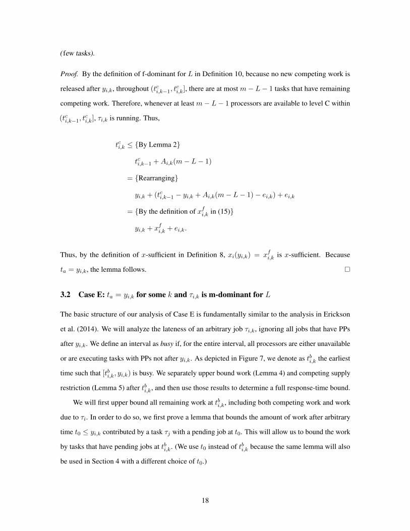
3.2 Case E: ta = yi,k for some k and τi,k is m-dominant for L
The basic structure of our analysis of Case E is fundamentally similar to the analysis in Erickson
et al. (2014). We will analyze the lateness of an arbitrary job τi,k, ignoring all jobs that have PPs
after yi,k. We define an interval as busy if, for the entire interval, all processors are either unavailable
or are executing tasks with PPs not after yi,k. As depicted in Figure 7, we denote as tbi,k the earliest
time such that [tbi,k, yi,k) is busy. We separately upper bound work (Lemma 4) and competing supply
restriction (Lemma 5) after tbi,k, and then use those results to determine a full response-time bound.
We will first upper bound all remaining work at tbi,k, including both competing work and work
due to τi. In order to do so, we first prove a lemma that bounds the amount of work after arbitrary
time t0 ≤ yi,k contributed by a task τj with a pending job at t0. This will allow us to bound the work
by tasks that have pending jobs at tbi,k. (We use t0 instead of tbi,k because the same lemma will also
be used in Section 4 with a different choice of t0.)
18
Figure 7: Example depicting tbi,k when m = 4.
Lemma 3. If there is a pending job of τj at arbitrary time t0 ≤ yi,k, then denote as τj,` the earliest
job of τj pending at t0. The total remaining work at time t0 for jobs of τj with PPs not later than yi,k
is erj,`(t0) +Dej (bj,`, yi,k).
Proof. By the definition of bj,` in Definition 5 and the definition of Ti in (5), any job of τj after τj,`
must be released no sooner than bj,`. Therefore, by Definition 6, the total work from such jobs with
PPs not later than yi,k is Dej (bj,`, yi,k). Adding erj,`(t0) for the remaining work due to τj,` yields the
lemma.
We now bound all remaining work at tbi,k, including that due to τi.
Lemma 4. The remaining work at tbi,k for jobs with PPs not later than yi,k is
Wi,k ,∑
τj,`∈θi,k
(erj,`(tbi,k) +De
j (bj,`, yi,k)) +∑τj∈θi,k
Dej (t
bi,k, yi,k). (16)
where θi,k is the set of jobs τj,` such that τj,` is the earliest pending job of τj at tbi,k, rj,` < tbi,k, and
yj,` ≤ yi,k, and θi,k is the set of tasks that do not have jobs in θi,k.
Proof. As before, we ignore any jobs that have PPs after yi,k. We bound the work remaining for
each task τj at tbi,k, depending on whether it has a pending job at tbi,k with a release before tbi,k.
Case 1: τj has no pending job at tbi,k with a release before tbi,k. If no job of τj with PP at or before
yi,k is pending at tbi,k, or if the earliest pending job of τj at tbi,k is released at tbi,k, then all relevant
work remaining for τj at tbi,k comes from jobs τj,` with tbi,k ≤ rj,` ≤ yj,` ≤ yi,k. Thus, by the
19
definition of Dej (t
bi,k, yi,k) in Definition 6, there are
Dej (t
bi,k, yi,k) (17)
units of such work. Furthermore, such a task is in θi,k by the definition of θi,k in the statement of the
lemma.
Case 2: τj has a pending job at tbi,k with a release before tbi,k. Denote as τj,` the earliest pending
job of τj at tbi,k. By Lemma 3 (with t0 = tbi,k), the remaining work for τj at tbi,k is
erj,`(tbi,k) +De
j (bj,`, yi,k). (18)
Furthermore, τj,` is in θi,k by the definition of θi,k in the statement of the lemma.
Summing over all tasks, using (17) or (18) as appropriate, yields Wi,k by (16).
We next consider supply restriction, accounting for it as if it were competing work. There is one
significant difference between supply restriction and competing work. Under GEL-v scheduling,
once a job has reached its PP, no new competing work can arrive. However, new supply restriction
can continue to be encountered until the job completes. Because we assume that the available supply
is infinite when extended into the future, every job must eventually complete. Therefore, by the
definition of x-sufficient in Definition 8, we have that each τi,k completes by time yi,k+xi(yi,k)+ei,k
for some x-sufficient xi(yi,k). We reference such a xi(yi,k) in the following lemma, and instantiate
it to a specific value in Theorem 5 below.
Lemma 5. For arbitrary job τi,k and x-sufficient xi(yi,k), at most
(m− utot)((yi,k − tbi,k) + xi(yi,k) + ei,k) +Oi,k,
units of competing supply restriction exist after tbi,k, where
Oi,k ,∑Pp∈P
op(tbi,k, t
ci,k). (19)
20
Proof. By the definition of βp(tbi,k, tci,k) in Definition 7, the amount of time that Pp is not available
to level C over [tbi,k, tci,k) is
(tci,k − tbi,k)− βp(tbi,k, tci,k)
≤ By (9)
(tci,k − tbi,k)− up · (tci,k − tbi,k) + op(tbi,k, t
ci,k).
= Rearranging
(1− up) · (tci,k − tbi,k) + op(tbi,k, t
ci,k).
This quantity upper bounds the competing supply restriction on Pp. Summing over all processors,
the total amount of competing supply restriction on all processors is at most
∑Pp∈P
((1− up) · (tci,k − tbi,k) + op(tbi,k, t
ci,k))
= Rearranging( ∑Pp∈P
1−∑Pp∈P
up
)· (tci,k − tbi,k) +
∑Pp∈P
op(tbi,k, t
ci,k)
= Because there are m processors in P , by the definition of utot in (10), and by the definition
of Oi,k in (19)
(m− utot) · (tci,k − tbi,k) +Oi,k
≤ By the definition of x-sufficient in Definition 8
(m− utot) · (yi,k + xi(yi,k) + ei,k − tbi,k) +Oi,k
= Rearranging
(m− utot) · ((yi,k − tbi,k) + xi(yi,k) + ei,k) +Oi,k.
We now compute a lateness bound that accounts for both work and competing supply restriction.
As discussed earlier, we will analyze the behavior of the system after yi,k, when new job arrivals
cannot preempt τi,k.
21
We will now consider how to bound the total length of sub-intervals of Type 1 as described
earlier, during which τi does not execute because all processors are occupied by competing work
or supply restriction. We will do so by bounding the total amount of competing work and supply
restriction over [yi,k, tci,k). Recall that in Lemmas 4–5, competing work and supply restriction were
determined over [tbi,k, tci,k) rather than [yi,k, t
ci,k). The following property will allow us to transition
to reasoning about [yi,k, tci,k). It holds by the definition of tbi,k.
Property 4. m · (yi,k − tbi,k) units of work and/or supply restriction complete in [tbi,k, yi,k).
We now bound the amount of competing work and supply restriction in [yi,k, tci,k).
Lemma 6. For arbitrary τi,k, at most
Wi,k −Ri,k + (m− utot)(xi(yi,k) + ei,k) +Oi,k − eri,k(yi,k)− epi,k
units of competing work and supply restriction remain at yi,k, where
Ri,k , utot(yi,k − tbi,k). (20)
Proof. By Lemma 4, the total amount of remaining work at tbi,k is Wi,k. Adding this to the bound on
competing supply restriction in Lemma 5, there are at most
Wi,k + (m− utot)((yi,k − tbi,k) + xi(yi,k) + ei,k) +Oi,k
units of work and supply restriction after tbi,k. Of this work and supply restriction, by Property 4, the
amount remaining at yi,k is at most
Wi,k + (m− utot)((yi,k − tbi,k) + xi(yi,k) + ei,k) +Oi,k −m · (tbi,k − yi,k)
= Rearranging
Wi,k − utot · (yi,k − tbi,k) + (m− utot) · (xi(yi,k) + ei,k) +Oi,k
= By the definition of Ri,k in (20)
Wi,k −Ri,k + (m− utot) · (xi(yi,k) + ei,k) +Oi,k. (21)
22
Of this remaining work and supply restriction, by the definition of epi,k in Definition 9, epi,k units are
due to jobs of τi prior to τi,k, and by the definition of eri,k(yi,k) in Definition 3, eri,k(yi,k) units are
due to τi,k itself. The lemma follows immediately.
We now bound the completion time of τi,k.
Lemma 7. If τi,k is m-dominant for L and xi(yi,k) is x-sufficient, then
tci,k ≤ yi,k +Wi,k −Ri,k + (m− utot)(xi(yi,k) + ei,k) +Oi,k − ei,k + Lepi,k
m+ ei,k.
Proof. By the definition of m-dominant for L in Definition 11, there are always at least m− L− 1
units of competing work or supply restriction that must run concurrently with τi whenever jobs of
τi prior to τi,k are running after yi,k. (This statement is vacuously true if no jobs of τi prior to τi,k
run after yi,k.) In other words, during any instant within any sub-interval of Type 2 (as depicted in
Figure 5(b)), there are at least m− L− 1 processors executing competing work or supply restriction.
Recall that, by the definition of “Type 2” and the definition of epi,k in Definition 9, the total length of
such intervals is epi,k.
By Lemma 6 there can be at most
c ,Wi,k −Ri,k + (m− utot)(xi(yi,k) + ei,k) +Oi,k − eri,k(yi,k)
− epi,k − (m− L− 1)epi,k
= Rearranging
Wi,k −Ri,k + (m− utot)(xi(yi,k) + ei,k) +Oi,k − eri,k(yi,k) + (L−m)epi,k (22)
units of computing work and supply restriction after yi,k that do not run concurrently with jobs of τi
prior to τi,k. This bound includes all work and/or supply restriction in sub-intervals of Type 1. All m
processors are occupied by work or supply restriction in such sub-intervals, so the total length of
such sub-intervals is at most c/m.
Recall from Definition 9 that the total length of Type 2 sub-intervals (in which jobs of τi prior to
τi,k execute) is defined to be epi,k, and the total length of Type 3 sub-intervals (in which τi,k runs) is
eri,k(yi,k).
23
Therefore,
tci,k ≤ Adding the total length of each type of sub-interval to yi,k
yi,k +c
m+ epi,k + eri,k(yi,k)
= By (22)
yi,k +Wi,k −Ri,k + (m− utot)(xi(yi,k) + ei,k) +Oi,k − eri,k(yi,k) + (L−m)epi,k
m
+ epi,k + eri,k(yi,k)
= Rearranging
yi,k +Wi,k −Ri,k + (m− utot)(xi(yi,k) + ei,k) +Oi,k + Lepi,k
m+m− 1
m· eri,k(yi,k)
≤ Because eri,k(yi,k) ≤ ei,k and m ≥ 1
yi,k +Wi,k −Ri,k + (m− utot)(xi(yi,k) + ei,k) +Oi,k + Lepi,k
m+m− 1
m· ei,k
= Rearranging
yi,k +Wi,k −Ri,k + (m− utot)(xi(yi,k) + ei,k) +Oi,k − ei,k + Lepi,k
m+ ei,k.
The next lemma provides the actual bound on xi(ta).
Theorem 5. If ta = yi,k for some k, tci,k > yi,k + ei,k and τi,k is m-dominant for L, then xi(ta) =
xmi,k is x-sufficient, where
xmi,k ,Wi,k −Ri,k + (m− utot − 1)ei,k +Oi,k + Lepi,k
utot(23)
(many tasks).
Proof. We let
xti,k , tci,k − ei,k − yi,k (24)
(tight). Rearranging,
tci,k = yi,k + xti,k + ei,k. (25)
24
Because tci,k > yi,k + ei,k, by (24)–(25) and the definition of x-sufficient in Definition 8, xi(yi,k) =
xti,k is x-sufficient.
Therefore, by Lemma 7 with xi(yi,k) = xti,k and (25),
xti,k ≤Wi,k −Ri,k + (m− utot) · (xti,k + ei,k) +Oi,k − ei,k + L · epi,k
m.
We solve for xti,k. First, we will add utot−mm · xti,k to both sides, which yields
utotm· xti,k ≤
Wi,k −Ri,k + (m− utot) · ei,k +Oi,k − ei,k + L · epi,km
.
We then multiply both sides by utotm . Because utot > 0 and m > 0,
xti,k ≤Wi,k −Ri,k + (m− utot) · ei,k +Oi,k − ei,k + L · epi,k
utot
= Rearranging
Wi,k −Ri,k + (m− utot − 1) · ei,k +Oi,k + L · epi,kutot
= By the definition of xmi,k in (23)
xmi,k.
Because xi(yi,k) = xti,k is x-sufficient, by Property 3 with c0 = xti,k and c1 = xmi,k, xi(yi,k) = xmi,k
is x-sufficient. Because ta = yi,k, the lemma follows.
4 Dissipation Bounds
The response-time analysis provided in Section 3 is very general, in order to provide an accurate
characterization of the behavior in overload situations. In particular, it can even be used to analyze the
behavior of systems where no per-task bound on response times exists. In this section, we consider
systems that have per-task response time bounds in the absence of overload. In other words, each
task has some constant xsi (1) such that, if s(t) = 1 for all t, then xi(t) = xsi (1) is x-sufficient for all
τi and time t. (The reason for the “1” argument will be described later.) In this section, we analyze a
system where an overload actually does occur, but the overload is transient. This situation is similar
25
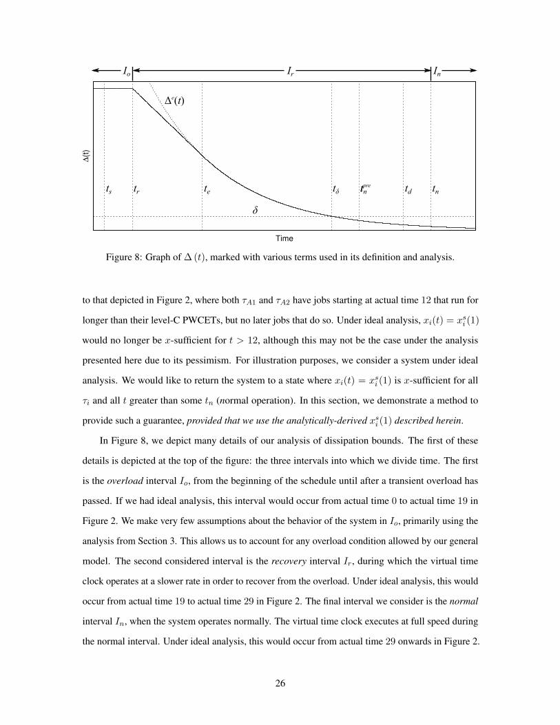
∆(t
)
Time
Δe(t)
Io Ir In
tr te tδ tntpre td tn
δ
ts
Figure 8: Graph of ∆ (t), marked with various terms used in its definition and analysis.
to that depicted in Figure 2, where both τA1 and τA2 have jobs starting at actual time 12 that run for
longer than their level-C PWCETs, but no later jobs that do so. Under ideal analysis, xi(t) = xsi (1)
would no longer be x-sufficient for t > 12, although this may not be the case under the analysis
presented here due to its pessimism. For illustration purposes, we consider a system under ideal
analysis. We would like to return the system to a state where xi(t) = xsi (1) is x-sufficient for all
τi and all t greater than some tn (normal operation). In this section, we demonstrate a method to
provide such a guarantee, provided that we use the analytically-derived xsi (1) described herein.
In Figure 8, we depict many details of our analysis of dissipation bounds. The first of these
details is depicted at the top of the figure: the three intervals into which we divide time. The first
is the overload interval Io, from the beginning of the schedule until after a transient overload has
passed. If we had ideal analysis, this interval would occur from actual time 0 to actual time 19 in
Figure 2. We make very few assumptions about the behavior of the system in Io, primarily using the
analysis from Section 3. This allows us to account for any overload condition allowed by our general
model. The second considered interval is the recovery interval Ir, during which the virtual time
clock operates at a slower rate in order to recover from the overload. Under ideal analysis, this would
occur from actual time 19 to actual time 29 in Figure 2. The final interval we consider is the normal
interval In, when the system operates normally. The virtual time clock executes at full speed during
the normal interval. Under ideal analysis, this would occur from actual time 29 onwards in Figure 2.
26
In order to provide boundaries between these intervals, we define several variables. ts is defined
to be the time at which the virtual clock actually slows. tn will be defined as the time when the
virtual clock can be returned to a normal speed. We note that the virtual clock can be returned to a
normal speed at a later time without compromising correctness. We assume that the virtual clock is
slowed to a constant speed sr from ts to tn, as specified in the following property.
Property 5. For all t ∈ [ts, tn), s(t) = sr < 1.
In Figure 2, sr = 0.5. Similarly, the following property describes the behavior of the virtual
clock after the system has returned to normal.
Property 6. If t ∈ In, then s(t) = 1.
Because the speed of the virtual clock is determined by the operating system, it is always possible
to ensure that both properties hold.
Although the virtual clock is actually slowed at time ts, for our analysis within Ir, it will often be
convenient to assume that that the virtual clock has been operating at a constant rate for a period of
time. Furthermore, we will also need to assume that overload does not occur in the recovery interval
in order to make guarantees, even though unexpected overload could continue to occur even after ts.
Therefore, we define the start of the recovery interval, denoted tr, as the earliest time that satisfies all
of the following properties.
Property 7. If any τi,k is pending at tr, then yi,k ≥ ts.
Property 8. Each task τi has a constant Ci ≤ Ti such that for any τi,k, if tci,k ≥ tr, then ei,k ≤ Ci.
Property 9. For each Pp, there is some constant σp such that if tr ≤ t0 ≤ t1, then op(t0, t1) ≤ upσp.
Property 8 states that Ci is the worst-case execution time for any job of τi that influences our
analysis within Ir ∪ In. Property 9 eliminates some of the generality of our supply model from tr
onward, so that our supply model becomes identical to that used in Leontyev and Anderson (2010)
holds from tr onward, in Ir ∪ In. In light of Property 8, we define a task’s base utilization (with
respect to virtual time)
Uvi =CiTi
(26)
27
and its Ir utilization (with respect to actual time in Ir)
U ri = Uvi · sr. (27)
Observe that the utilization of τi with respect to actual time in In is simply Uvi , because s(t) = 1 for
all t ∈ In.
With these definitions in place, we formally define the extent of each interval.
Io , [0, tr), (28)
Ir , [tr, tn), (29)
In , [tn,∞). (30)
If we can guarantee that xi(t) = xsi (1) is x-sufficient for t ∈ In under Properties 5–9, then we
define a dissipation bound as the length of Ir, i.e., tn − tr.
Whenever s(t) remains constant over an interval (as it does over Ir and In), it is possible to
correctly choose xi(t) such that it asymptotically approaches a constant value. We will below define
this (task-dependent) constant value as xsi (sI), where sI is the constant value of s(t) (sr in Ir and 1 in
In). We will then define a task-independent function ∆ (t) that guarantees that xi(t) = xsi (sr)+∆ (t)
is x-sufficient for every τi and time t ∈ Ir. ∆ (t) is graphed in Figure 8.
Recall that, in Section 3, L was arbitrary for each τi,k. Our analysis will require us to choose a
particular L for each task, so in Section 4.1 below, we discuss how to make this choice. In Section 4.2,
we then turn our attention to formally defining xsi (sI) and ∆ (t). Then, in Section 4.3, we formally
prove that xi(ta) = xsi (sr) + ∆ (ta) is x-sufficient for ta ∈ Ir. In Section 4.4 we then upper bound
tn. Finally, in Section 4.5, we formally prove that xi(t) = xsi (1) is x-sufficient for t ∈ In.
4.1 Choosing L
In Section 3, L was arbitrary for any τi,k. In this subsection, we will choose a specific per-task Li
that will take the place of L in several of our bounds. Because Li will appear in our definition of
xsi (sI), we first describe its selection here. We will then define xsi (sI) and ∆ (t) in Section 4.2.
28
The choice of L appears in the definition of xmi,k in (23), in the term Lepi,k, and in the definition
of xfi,k in (15), in the argument to Ai,k(m− L− 1). In order to analyze xfi,k, we first upper bound
Ai,k(m−L− 1) in the case that will be relevant to our choice of xsi (sI). The following lemma does
so, using arbitrary v = m− L− 1 to match the notation used in Lemma 2.
Lemma 8. Let v be an integer with 0 ≤ v < m, and let
Arni (v) ,
Ci+
∑Pp∈Θrn
upσp
1−v+∑Pp∈Θrn
upIf 1− v +
∑Pp∈Θrn
up > 0
∞ Otherwise,(31)
(for Ir and In) where Θrn is the set of v processors that minimizes Arni (v). Then, if k ≥ 0 and
tci,k−1 > tr. Ai,k(v) ≤ Arni (v) and Ai,k(v)− ei,k ≤ Arni (v)− Ci.
Proof. If Arni (v) =∞, then the lemma holds. Furthermore, if Ai,k(v) =∞, then by (13), for any
choice of v processors Θ, 1− v +∑
Pp∈Θ up ≤ 0. Therefore, Arni (v) =∞, and the lemma holds.
Thus, we assume that Arni (v) is finite, implying by (31) that
1− v +∑
Pp∈Θrn
up > 0, (32)
and that Ai,k(v) is finite, implying by (13) that
1− v +∑Pp∈Θ
up > 0. (33)
Additionally,
1− v +∑
Pp∈Θrn
up ≤ Because each up ≤ 1
1− v +∑
Pp∈Θrn
1
= Because there are v processors in Θrn
1. (34)
29
We have
Arni (v) = By the definition of Arni (v) in (31) and by (32)
Ci +∑
Pp∈Θrnupσp
1− v +∑
Pp∈Θrnup
≥ By Property 9 and (32)
Ci +∑
Pp∈Θrnoi(t
ci,k−1, t
ci,k)
1− v +∑
Pp∈Θrnup
≥ By Property 8 and (32)
ei,k +∑
Pp∈Θrnoi(t
ci,k−1, t
ci,k)
1− v +∑
Pp∈Θrnup
≥ Because Θ (as defined in Lemma 2) is chosen to minimize Ai,k(v), and by (32)
Ai,k(v). (35)
Similarly,
Arni (v)− Ci = By the definition of Arni (v) in (31) and by (32)
Ci +∑
Pp∈Θrnupσp
1− v +∑
Pp∈Θrnup− Ci
≥ By Property 9 and (32)
Ci +∑
Pp∈Θrnoi(t
ci,k−1, t
ci,k)
1− v +∑
Pp∈Θrnup
− Ci
≥ By Property 8 and (32) and (34)
ei,k +∑
Pp∈Θrnoi(t
ci,k−1, t
ci,k)
1− v +∑
Pp∈Θrnup
− ei,k
≥ Because Θ (as defined in Lemma 2) is chosen to minimize Ai,k(v), and by (32)
Ai,k(v)− ei,k. (36)
We now define our choice of Li.
30
Definition 12. For each τi, Li is the smallest integer such that 0 ≤ Li < m and Arni (m−Li− 1) ≤
Ti.
Such an integer must exist, because
Arni (m− (m− 1)− 1) = Rearranging
Arni (0)
= By the definition of Arni (0) in (31)
Ci
≤ By Property 8
Ti.
4.2 Defining xsi (sI) and ∆ (t)
In this subsection, we define xsi (sI) and ∆ (t). We will prove in Section 4.3 below that they can be
used to obtain x-sufficient bounds.
We first define xsi (sI). Its definition is implicit — xsi (sI) appears on both sides of (37) below.
In Appendix B, we discuss how to use linear programming to determine the specific value of xsi (sI)
if it exists. In Appendix B, we also show that if xsi (1) exists, then xsi (sI) must exist for all sI ≤ 1.
Definition 13.
xsi (sI) , max
0,
( ∑m−1 largest
(Cj + Uvj · sI · xsj(sI)− Sj) +∑τj∈τ
Sj + (m− utot − 1)Ci
+Orn + Li · Uvi · sI · xsi (sI))/utot
. (37)
where
Si , Ci
(1− Yi
Ti
), (38)
and
Orn ,∑Pp∈P
upσp (39)
(for intervals Ir and In).
31
In order to prove that xi(ta) = xsi (1) is x-sufficient for ta ∈ In, it is necessary that xsi (1) exist.
In Appendix B, we show that this occurs if the provided linear program is feasible, and that the
following condition is sufficient for feasibility.
Property 10. ∑m−1 largest
Uvj + maxτi∈τ
Li · Uvi < utot.
If Property 10 is not satisfied, then the methods provided in this paper cannot provide dissipation
bounds. Furthermore, our analysis also assumes the following property, without which bounded
response times cannot be guaranteed even in the absence of overload.
Property 11. ∑τj∈τ
Uvj ≤ utot.
We next define ∆ (t). The definition of ∆ (t) uses several upper bounds of quantities from
Section 3. We will justify the correctness of these upper bounds in Section 4.3. We will describe each
segment of ∆ (t), as depicted in Figure 8, from left to right. We will provide necessary definitions as
we proceed.
Observe in Figure 8 that for t ≤ tr, ∆ (t) is constant. We will denote this constant value as λ,
and we will define λ below. First, we describe a function closely related to xi(t) that will be used in
defining λ. Observe in Definition 8 that the provided equation must hold for all τi,k with yi,k ≤ t.
We define xi(t) by changing this precondition to a strict inequality, in order to handle an edge case in
our analysis.
Definition 14. xi(t) is x-sufficient if xi(t) ≥ 0 and for all τi,k with yi,k < t,
tci,k ≤ t+ xi(t) + ei,k.
With this definition in place, we now define λ.
λ , max
maxτi∈τ
xi(tr)− xsi (sr) +Arni (m− Li − 1),
δ,
32
maxτi,k∈ψ
(W oi,k −Roi,k + (m− utot − 1)ei,k +Ooi,k +Orn + Li · U ri · xsi (sr)
utot − Li · U ri
),
maxτi,k∈κ
(xi(yi,k)− xsi (sr)),
0
, (40)
where each xi(tr) is x-sufficient,
δ , minτi∈τ
xsi (1)− xsi (sr), (41)
ψ is the set of jobs with yi,k ∈ Ir ∪ In and tbi,k ∈ Io, κ is the set of jobs with yi,k ∈ Io and
tci,k ∈ Io ∪ Ir, each xi(yi,k) is x-sufficient,
W oi,k ,Wi,k −
∑τj∈τ
Dej (tr, yi,k) +
∑τj∈τ
Sj (42)
(for jobs with tbi,k ∈ Io), and
Roi,k , utot · (tr − tbi,k) (43)
Ooi,k ,∑Pp∈P
op(tbi,k, tr) (44)
(each for Io).
Observe in Figure 8 that, from tr to te (switch to exponential), ∆ (t) is linear. We define this
segment as its own function
∆` (t) , φ · (t− tr) + λ (45)
(linear), where
φ , max
maxτj∈τ
(sr ·Arnj (m− Lj − 1)
Ti− 1
),
∑τj∈τ U
rj − utot
utot
. (46)
As can be seen in Figure 8, from te onward, ∆ (t) decays exponentially. We will also define this
segment as its own function,
∆e (t) , ∆` (te) · qt−teρ (47)
33
A. ta < yi,0 (Lemma 14).
B. ta = yi,k for some k and tci,k ≤ yi,k + ei,k (Lemma 15).
C. ta ∈ (yi,k, yi,k+1) for some k (Lemma 21).
D. ta = yi,k for some k, tci,k > yi,k + ei,k, and τi,k is f-dominant for Li (Lemma 25).
E. ta = yi,k for some k, tci,k > yi,k + ei,k, and τi,k is m-dominant for Li (Lemma 49).
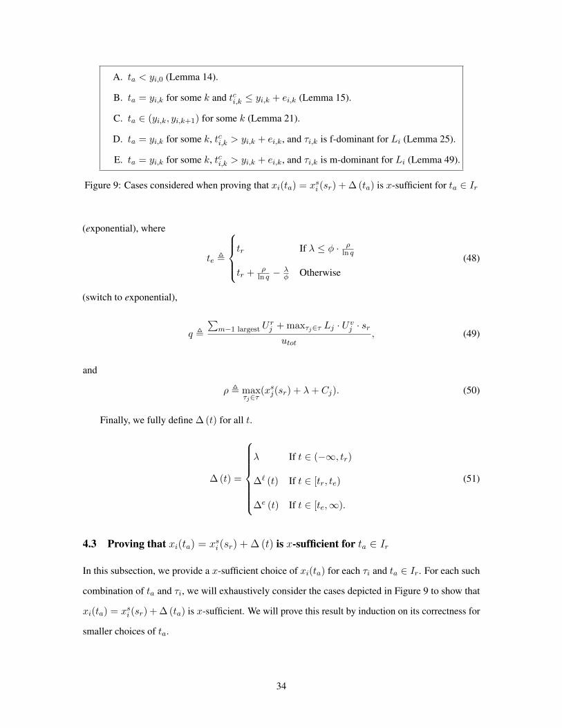
Figure 9: Cases considered when proving that xi(ta) = xsi (sr) + ∆ (ta) is x-sufficient for ta ∈ Ir
(exponential), where
te ,
tr If λ ≤ φ · ρ
ln q
tr + ρln q −
λφ Otherwise
(48)
(switch to exponential),
q ,
∑m−1 largest U
rj + maxτj∈τ Lj · Uvj · srutot
, (49)
and
ρ , maxτj∈τ
(xsj(sr) + λ+ Cj). (50)
Finally, we fully define ∆ (t) for all t.
∆ (t) =
λ If t ∈ (−∞, tr)
∆` (t) If t ∈ [tr, te)
∆e (t) If t ∈ [te,∞).
(51)
4.3 Proving that xi(ta) = xsi (sr) + ∆ (t) is x-sufficient for ta ∈ Ir
In this subsection, we provide a x-sufficient choice of xi(ta) for each τi and ta ∈ Ir. For each such
combination of ta and τi, we will exhaustively consider the cases depicted in Figure 9 to show that
xi(ta) = xsi (sr) + ∆ (ta) is x-sufficient. We will prove this result by induction on its correctness for
smaller choices of ta.
34
Furthermore, a necessary condition in Definition 8 for xi(t) to be x-sufficient is that xi(t) ≥ 0.
Lemma 13 below establishes that this is the case for xi(ta) = xsi (sr) + ∆ (ta) for arbitrary ta.
By the definition of xsi (sr) in (37), xsi (sr) is nonnegative. Therefore, showing that ∆ (ta) is also
nonnegative for arbitrary ta will be sufficient to prove Lemma 13.
By the definition of ∆ (ta) in (51), we will consider the three intervals (−∞, tr), [tr, te), and
[te,∞). ∆ (ta) is nonnegative for ta ∈ (−∞, tr), because by the definition of λ in (40), λ ≥ 0. We
thus consider ta ∈ [tr, te). In order to prove that ∆ (ta) is nonnegative in this case, we will show (in
Lemma 9) that ∆` (t) is decreasing over [tr, te), and (in Lemma 12) that ∆` (te) is nonnegative. The
result that ∆ (te) is nonnegative will also be used to prove that ∆ (ta) is nonnegative for ta ∈ [te,∞).
By the definition of ∆` (t) in (45), ∆` (t) is decreasing if and only if φ < 0. We now prove that
this is implied by Property 11.
Lemma 9. φ < 0.
Proof. By the definition of φ in (46), either φ =sr·Arnj (m−Lj−1)
Tj− 1 for some τj , or φ =∑
τj∈τUrj−utotutot
. We consider each of these cases.
Case 1: φ =sr·Arnj (m−Lj−1)
Tj− 1 for some τj . In this case, we have
φ =sr ·Arnj (m− Lj − 1)
Tj− 1
≤ By the definition of Lj in Definition 12sr · TjTj
− 1
= Cancelling
sr − 1
< By Property 5
0.
Case 2: φ =
∑τj∈τ
Urj−utotutot
. In this case, we have
φ =
∑τj∈τ U
rj − utot
utot
35

= By the definition of U rj in (27)∑τj∈τ (Uvj · sr)− utot
utot
< By Property 5∑τj∈τ U
vj − utot
utot
≤ By Property 11utot − utot
utot
= Simplifying
0.
We need to show that ∆` (te) is nonnegative. By the definition of te in (48), the value of te is
dependent on ln q. Thus, we first characterize the value of q.
Lemma 10. 0 < q < 1.
Proof. We first show that 0 < q. All variables that appear in the definition of q in (49) are nonnegative,
and U rj for each τj is strictly positive. Therefore, 0 < q.
We now show that q < 1. We have
q = By the definition of q in (49)∑m−1 largest U
rj + maxτj∈τ Lj · Uvj · srutot
= By the definition of U rj in (27)∑m−1 largest(U
vj · sr) + maxτj∈τ Lj · Uvj · sr
utot
< By Property 5∑m−1 largest U
vj + maxτj∈τ Lj · Uvjutot
≤ By Property 10utotutot
36
= Simplifying
1.
Also by the definition of te in (48), the value of te is also dependent on ρ. Thus, we also
characterize the value of ρ.
Lemma 11. ρ > 0.
Proof. We have
ρ = By the definition of ρ in (50)
maxτj∈τ
(xsj(sr) + λ+ Cj)
≥ By the definition of xsj(sr) in (37) and the definition of λ in (40)
maxτj∈τ
(Cj)
> Because each Cj > 0
0.
We finally show that ∆` (te) is nonnegative. Furthermore, the value of ∆` (te) and the identical
values of ∆ (te) and ∆e (te) are used in later proofs. For convenience, we consider all of these terms
in a single lemma.
Lemma 12.
∆ (te) = ∆e (te) = ∆` (te) = min
λ, φ · ρ
ln q
≥ 0.
Proof. We will demonstrate the equalities in the order they appear in the statement of the lemma.
First, we have
∆ (te) = By the definition of ∆ (te) in (51)
∆e (te)
37
= By the definition of ∆e (te) in (47)
∆` (te) · qte−teρ
= Simplifying
∆` (te) .
We now establish that ∆` (te) = minλ, φ · ρ
ln q
by considering two cases.
Case 1: λ ≤ φ · ρln q . In this case,
∆` (te) = By the definition of te in (48)
∆` (tr)
= By the definition of ∆` (tr) in (45)
φ · (tr − tr) + λ
= Simplifying
λ
= By the case we are considering
min
λ, φ · ρ
ln q
.
Case 2: λ > φ · ρln q . In this case,
∆` (te) = By the definition of te in (48)
∆`
(tr +
ρ
ln q− λ
φ
)= By the definition of ∆`
(tr + ρ
ln q −λφ
)in (45)
φ ·(tr +
ρ
ln q− λ
φ− tr
)+ λ
= Simplifying
φ · ρ
ln q
= By the case we are considering
38
min
λ, φ · ρ
ln q
.
Finally, we demonstrate that minλ, φ · ρ
ln q
≥ 0. By the definition of λ in (40), λ ≥ 0.
Furthermore, because φ < 0 by Lemma 9, 0 < q < 1 by Lemma 10, and ρ > 0 by Lemma 11,
φ · ρln q > 0. Therefore, min
λ, φ · ρ
ln q
≥ 0.
We are now ready to establish that xsi (sr) + ∆ (ta) ≥ 0. By Definition 8, this is a necessary
condition for xi(ta) = xsi (sr) + ∆ (ta) to be x-sufficient.
Lemma 13. For all ta, xsi (sr) + ∆ (ta) ≥ 0.
Proof. We first establish that ∆ (ta) ≥ 0. We consider three cases, depending on the value of ta.
Case 1: ta ∈ (−∞, tr). In this case,
∆ (ta) = By the definition of ∆ (ta) in (51)
λ
≥ By the definition of λ in (40)
0.
Case 2: ta ∈ [tr, te). In this case,
∆ (ta) = By the definitions of ∆ (ta) in (51) and of ∆` (ta) in (45)
φ · (ta − tr) + λ
= Rearranging
φ · (te − tr) + λ+ φ · (ta − te)
= By the definition of ∆` (te) in (45)
∆` (te) + φ · (ta − te)
> Because φ < 0 by Lemma 9 and ta < te
∆` (te)
≥ By Lemma 12
39
0.
Case 3: ta ∈ [te,∞). In this case,
∆ (ta) = By the definitions of ∆ (ta) in (51) and of ∆e (ta) in (47)
∆` (te) · qta−teρ
≥ Because ∆` (te) ≥ 0 by Lemma 12 and q > 0 by Lemma 10
0.
In any of the above cases, because xsi (sr) ≥ 0 by the definition of xsi (sr) in (37), xsi (sr) +
∆ (ta) ≥ 0.
We now show that xi(ta) = xsi (sr) + ∆ (ta) is x-sufficient by considering all the cases depicted
in Figure 9, which match those in Figure 3 in Section 3.
We first consider Case A in Figure 9, in which ta < yi,0.
Lemma 14. If ta < yi,0, then xi(ta) = xsi (sr) + ∆ (ta) is x-sufficient.
Proof. If ta < yi,0, then by Theorem 1, xi(ta) = 0 is x-sufficient. Furthermore, by Lemma 13,
xsi (sr) + ∆ (ta) ≥ 0. Therefore, by Property 3 with c0 = 0 and c1 = xsi (sr) + ∆ (ta), xi(ta) =
xsi (sr) + ∆ (ta) is x-sufficient.
The analysis of Case B in Figure 9 is simple.
Lemma 15. If ta = yi,k for some k and tci,k ≤ yi,k + ei,k, then xi(ta) = xsi (sr) + ∆ (ta) is
x-sufficient.
Proof. The lemma follows immediately from Theorem 2, Lemma 13, and Property 3 with c0 = 0
and c1 = xsi (sr) + ∆ (ta).
We next consider Case C in Figure 9, in which ta ∈ (yi,k, yi,k+1) for some k. For this case, as
well as most subsequent cases, correctness is proved from the fact that the value of ∆ (t) decreases
sufficiently slowly as t increases. Therefore, we will prove Lemma 20 below, which explicitly bounds
40
the decrease between two values of ∆ (t). Our analysis will be based on the following form of the
Fundamental Theorem of Calculus (FTC).
Fundamental Theorem of Calculus (FTC). If f(t) is continuous over [t0, t1] and f ′(t) is the
derivative of f(t) at all but finitely many points within [t0, t1], then
f(t1) = f(t0) +
∫ t1
t0
f ′(t) dt.
In order to use the FTC, we will demonstrate in Lemma 17 below that ∆ (t) is continuous over
all real numbers, and in Lemma 19 below we will provide a function ∆′ (t) that is equal to the
derivative of ∆ (t) at all but finitely many points. Lemma 19 also provides bounds on ∆′ (t) that are
used to prove Lemma 20. In several parts of our analysis throughout this section, the value of ∆ (tr)
and/or ∆` (tr) will be used. For convenience, we provide this value now as a separate lemma.
Lemma 16. ∆ (tr) = ∆` (tr) = λ.
Proof. We first establish that ∆ (tr) = ∆` (tr). By (48), either tr = te or tr < te. We consider each
of these two cases.
Case 1: te = tr. In this case,
∆ (tr) = ∆ (te)
= By Lemma 12
∆` (te)
= Because te = tr
∆` (tr) .
Case 2: tr < te. In this case, by the definition of ∆ (tr) in (51), ∆ (tr) = ∆` (tr).
To conclude the proof, note that
∆` (tr) = By the definition of ∆` (tr) in (45)
φ · (tr − tr) + λ
41
= Simplifying
λ.
The following property is a standard result in real analysis. (If t2 ≤ t1, then it holds vacuously.)
Property 12. For arbitrary t0, t1, t2, and continuous functions f(t) and g(t), if t1 > t0, ∆ (t) = f(t)
for t ∈ (t0, t1), ∆ (t) = g(t) for t ∈ [t1, t2), and f(t1) = g(t1), then ∆ (t) is continuous over [t1, t2).
We now use this property to prove that ∆ (t) is continuous over the reals, so that we can use the
FTC with f(t) = ∆ (t).
Lemma 17. ∆ (t) is continuous over all real numbers.
Proof. We first observe that, by the definition of ∆ (t) in (51), ∆ (t) is constant (and therefore
continuous) over (−∞, tr).
To prove that ∆ (t) is continuous over [tr,∞), we consider two cases, depending on the relation-
ship between λ and φ · ρln q .
Case 1: λ ≤ φ · ρln q . We will use Property 12 with t0 = −∞, t1 = tr, t2 = ∞, f(t) = λ, and
g(t) = ∆e (t). It is trivially the case that t1 > t0.
In this case, by the definition of te in (48),
tr = te. (52)
Therefore, by the definition of ∆ (t) in (51), ∆ (t) = λ = f(t) for t ∈ (t0, t1) = (−∞, tr) and
∆ (t) = ∆e (t) = g(t) for t ∈ [t1, t2) = [tr,∞), as desired.
f(t) is continuous because it is constant. g(t) is continuous by the definition of ∆e (t) in (47),
because exponential functions are continuous.
Finally, we show that
g(t1) = ∆e (tr)
= By (52)
42
∆e (te)
= By Lemma 12 and the case we are considering
λ
= f(t1). (53)
Therefore, all the preconditions for Property 12 are met, so ∆ (t) is continuous over [tr,∞).
Case 2: λ ≤ φ · ρln q . In this case, by the definition of te in (48), we have
tr < te. (54)
We first prove that ∆ (t) is continuous over [tr, te), using Property 12 with f(t) = λ, g(t) = ∆` (t),
t0 = −∞, t1 = tr, and t2 = te. It is trivially the case that t1 > t0. By the definition of ∆ (t) in (51),
∆ (t) = λ = f(t) for t ∈ (t0, t1) = (−∞, tr) and ∆ (t) = ∆` (t) = g(t) for t ∈ [t1, t2) = [tr, te).
f(t) is continuous because it is constant. g(t) is continuous by the definition of ∆` (t) in (45),
because linear functions are continuous. Furthermore,
g(t1) = ∆` (tr)
= By Lemma 16
λ
= f(t1).
Therefore, all the preconditions for Property 12 are met, so ∆ (t) is continuous over [tr, te).
We next prove that ∆ (t) is continuous over [te,∞) using Property 12 with f(t) = ∆` (t),
g(t) = ∆e (t), t0 = tr, t1 = te, and t2 = ∞. By (54), t1 > t0. By the definition of ∆ (t) in
(51), ∆ (t) = ∆` (t) = f(t) for t ∈ (t0, t1) ⊂ [tr, te) and ∆ (t) = ∆e (t) = g(t) for t ∈ [t1, t2) =
[te,∞). f(t) is continuous by the definition of ∆` (t) in (45), because linear functions are continuous.
g(t) is continuous by the definition of ∆e (t) in (47), because exponential functions are continuous.
43
Furthermore,
g(t1) = ∆e (te)
= By Lemma 12
∆` (te)
= f(t1).
Therefore, all the preconditions for Property 12 are met, so ∆ (t) is also continuous over [te,∞).
We reasoned above that ∆ (t) is continuous over [tr, te), so ∆ (t) is continuous over [tr,∞).
In order to use the FTC, we must also provide a function ∆′ (t) that is equal to the derivative
of ∆ (t) at all but finitely many points. Both for the purposes of determining ∆′ (t), and for a later
proof, we must reason about the derivative of ∆e (t). The following lemma provides a necessary
property of that derivative.
Lemma 18. Let ∆e′ (t) be the derivative of ∆e (t) with respect to t. If t ≥ te, then 0 ≥ ∆e′ (t) ≥ φ.
Proof. If t ≥ te, then we have
∆e′ (t) = By the definition of ∆e (t) in (47) and differentiationln q
ρ·∆` (te) · q
t−teρ
≥ By Lemma 12, because 0 < q < 1 by Lemma 10 so that ln q < 0ln q
ρ· φ · ρ
ln q· q
t−teρ
= Rearranging
φ · qt−teρ . (55)
The lemma follows from (55), because φ < 0 by Lemma 9, 0 < q < 1 by Lemma 10, and
t ≥ te.
We finally provide the derivative of ∆ (t), except at t = tr and t = te (finitely many points), and
provide bounds on the resulting ∆′ (t).
44
Lemma 19. Let
∆′ (t) ,
0 If t ∈ (−∞, tr)
φ If t ∈ [tr, te)
∆e′ (t) If t ∈ [te,∞).
(56)
∆′ (t) is the derivative of ∆ (t) everywhere except at t = tr and at t = te. Furthermore, for all t,
φ ≤ ∆′ (t) ≤ 0.
Proof. We prove the lemma for arbitrary t, considering each of the three intervals that occur in the
definition of ∆ (t) in (51) and in the definition of ∆′ (t) in (56).
Case 1: t ∈ (−∞, tr). In this case, by the definition of ∆′ (t) in (56), ∆′ (t) = 0. Therefore, by
Lemma 9, φ < ∆′ (t) = 0. By the definition of ∆ (t) in (51), for t ∈ (−∞, tr), ∆ (t) = λ. Thus,
the derivative of ∆ (t) at t is ∆′ (t) = 0.
Case 2: t ∈ [tr, te). In this case, by the definition of ∆′ (t) in (56), ∆′ (t) = φ. Therefore, by
Lemma 9, ∆′ (t) = φ < 0. By the definition of ∆ (t) in (51), for t ∈ [tr, te), ∆ (t) = ∆` (t).
Therefore, by the definition of ∆` (t) in (45), if t 6= tr, then the derivative of ∆ (t) at t is φ = ∆′ (t).
Case 3: t ∈ [te,∞). In this case, by the definition of ∆′ (t) in (56), ∆′ (t) = ∆e′ (t). By Lemma 18,
φ ≤ ∆e′ (t) < 0. Therefore, φ ≤ ∆′ (t) < 0. By the definition of ∆ (t) in (51), for t ∈ [te,∞),
∆ (t) = ∆e (t). Therefore, by the definition of ∆e (t) in (47) and the definition of ∆e′ (t) as the
derivative of ∆e (t), if t 6= te, then the derivative of ∆ (t) at t is ∆e′ (t) = ∆′ (t).
We can now provide bounds on the value of ∆ (t1) relative to ∆ (t0) for arbitrary t0 ≤ t1, as
required for the proof of Lemma 21 and several later lemmas.
Lemma 20. For arbitrary t0 ≤ t1,
∆ (t0) ≥ ∆ (t1) ≥ ∆ (t0) + φ · (t1 − t0).
Proof. We have
∆ (t1) = By the FTC with f(t) = ∆ (t), and by Lemmas 17 and 19
45
∆ (t0) +
∫ t1
t0
∆′ (t) dt
≤ By Lemma 19
∆ (t0) +
∫ t1
t0
0 dt
= Rearranging
∆ (t0) .
Also,
∆ (t1) = By the FTC with f(t) = ∆ (t), and by Lemmas 17 and 19
∆ (t0) +
∫ t1
t0
∆′ (t) dt
≥ By Lemma 19
∆ (t0) +
∫ t1
t0
φdt
= Rearranging
∆ (t0) + φ · (t1 − t0).
We now provide the lemma that addresses Case C in Figure 9.
Lemma 21. If ta ∈ Ir, ta ∈ (yi,k, yi,k+1) for some k, and xi(yi,`) = xsi (sr)+∆ (yi,`) is x-sufficient
for all τi,` such that yi,` ∈ [tr, ta), then xi(ta) = xsi (sr) + ∆ (ta) is x-sufficient.
Proof. Observe that τi,k is the last job of τi released prior to ta. We consider two cases, depending
on the location of yi,k.
Case 1: yi,k < tr. Let xi(tr) be the value used in the definition of λ in (40). We have
tci,k ≤ By the definition of x-sufficient in Definition 14
tr + xi(tr) + ei,k
≤ Rearranging
46
tr + xsi (sr) + xi(tr)− xsi (sr) + ei,k
≤ By the definition of λ in (40)
tr + xsi (sr) + λ+ ei,k
= By Lemma 16
tr + xsi (sr) + ∆ (tr) + ei,k
= Rearranging
ta + xsi (sr) + ∆ (tr)− (ta − tr) + ei,k
≤ By the definition of φ in (46)
ta + xsi (sr) + ∆ (tr) + φ · (ta − tr) + ei,k
≤ By Lemma 20 with t0 = tr and t1 = ta
ta + xsi (sr) + ∆ (ta) + ei,k. (57)
Therefore, by the definition of x-sufficient in Definition 8, xi(ta) = xsi (sr) + ∆ (ta) is x-sufficient.
Case 2: yi,k ≥ tr. We have
xsi (sr) + ∆ (ta) ≥ By Lemma 20 with t0 = yi,k and t1 = ta
xsi (sr) + ∆ (yi,k) + φ · (ta − yi,k)
≥ By the definition of φ in (46)
xsi (sr) + ∆ (yi,k)− (ta − yi,k).
By the statement of the lemma, xi(yi,k) = xsi (sr) + ∆ (yi,k) is x-sufficient, so by Theorem 3,
xi(ta) = xsi (sr) + ∆ (yi,k) − (ta − yi,k) is x-sufficient. Therefore, by Property 3 with c0 =
xsi (sr)+∆ (yi,k)−(ta−yi,k) and c1 = xsi (sr)+∆ (ta), xi(ta) = xsi (sr)+∆ (ta) is x-sufficient.
We now consider Case D in Figure 9, where ta = yi,k for some k, tci,k > yi,k + ei,k, and τi,k
is f-dominant for Li. In this case, by the definition of f-dominant for Li in Definition 10, k > 0,
and thus τi,k−1 exists. In Lemma 22, we consider the case that yi,k−1 ∈ Io, and in Lemma 24, we
consider the case that yi,k−1 ∈ Ir.
47
Lemma 22. If ta ∈ Ir, ta = yi,k for some τi,k, τi,k is f-dominant for Li, and yi,k−1 ∈ Io, then
xi(ta) = xsi (sr) + ∆ (ta) is x-sufficient.
Proof. We have
xsi (sr) + ∆ (ta)
= Because ta = yi,k
xsi (sr) + ∆ (yi,k)
≥ By Lemma 20 with t0 = tr and t1 = yi,k
xsi (sr) + ∆ (tr) + φ · (yi,k − tr)
= By Lemma 16
xsi (sr) + λ+ φ · (yi,k − tr)
≥ By the definition of λ in (40)
xsi (sr) + xi(tr)− xsi (sr) +Arni (m− Li − 1) + φ · (yi,k − tr)
= Rearranging
tr + xi(tr) + ei,k−1 +Arni (m− Li − 1)− ei,k−1 − tr + φ · (yi,k − tr)
≥ By the definition of x-sufficient in Definition 14, because yi,k−1 < tr
tci,k−1 +Arni (m− Li − 1)− ei,k−1 − tr + φ · (yi,k − tr)
≥ By the definition of φ in (46)
tci,k−1 +Arni (m− Li − 1)− ei,k−1 − tr +
(sr ·Arni (m− Li − 1)
Ti− 1
)· (yi,k − tr)
= Rearranging
tci,k−1 − yi,k +Arni (m− Li − 1)− ei,k−1 +sr ·Arni (m− Li − 1)
Ti· (yi,k − tr)
≥ Because sr ≥ 0, Arni (m− Li − 1) > 0, Ti > 0, and yi,k > tr
tci,k−1 − yi,k +Arni (m− Li − 1)− ei,k−1
≥ By the definition of f-dominant for Li in Definition 10 and Property 8, because
tci,k−1 > yi,k ≥ tr
tci,k−1 − yi,k +Arni (m− Li − 1)− Ci
48
≥ By Lemma 8
tci,k−1 − yi,k +Ai,k(m− Li − 1)− ei,k
= By the definition of xfi,k in (15)
xfi,k. (58)
Furthermore, by the preconditions of the lemma and Theorem 4, xi(ta) = xfi,k is x-sufficient.
Therefore, by (58) and Property 3 with c0 = xfi,k and c1 = xsi (sr) + ∆ (ta), the lemma holds.
We next consider the case that yi,k−1 ∈ Ir in Lemma 24. We will explicitly consider the
difference between yi,k−1 and yi,k, based on the following lemma, which will also be used in
Section 4.5.
Lemma 23. For k > 0, v(yi,k) ≥ v(yi,k−1) + Ti.
Proof. We have
v(yi,k) = By the definition of Yi in (6)
v(ri,k) + Yi
≥ By the definition of Ti in (5)
v(ri,k−1) + Ti + Yi
= By the definition of Yi in (6)
v(yi,k−1) + Ti.
We now consider Case D when yi,k−1 ∈ Ir.
Lemma 24. If ta ∈ Ir, ta = yi,k for some τi,k, τi,k is f-dominant for Li, yi,k−1 ∈ Ir, and xi(yi,`) =
xsi (sr) + ∆ (yi,`) is x-sufficient for all τj,` with tr ≤ yi,` < yi,k, then xi(ta) = xsi (sr) + ∆ (ta) is
x-sufficient.
49
Proof. In Lemma 23 we considered the difference between yi,k and yi,k−1 in virtual time. We now
consider their difference in actual time.
(yi,k − yi,k−1) · sr = By Lemma 35
v(yi,k)− v(yi,k−1)
≥ By Lemma 23
v(yi,k−1) + Ti − v(yi,k−1)
= Rearranging
Ti.
Rearranging,
yi,k−1 ≤ yi,k −Tisr. (59)
Because xi(yi,`) + xsi (sr) + ∆ (yi,`) is x-sufficient for all yi,` < yi,k, by (59) and Lemma 21 with
ta = yi,k − Ti/sr, xi(yi,k − Ti/sr) = xsi (sr) + ∆ (yi,k − Ti/sr) is x-sufficient. Thus,
xsi (sr) + ∆ (ta)
= Because ta = yi,k
xsi (sr) + ∆ (yi,k)
≥ By Lemma 20 with t0 = yi,k − Tisr
and t1 = yi,k
xsi (sr) + ∆
(yi,k −
Tisr
)+ φ · Ti
sr
= Rearranging
yi,k −Tisr
+ xsi (sr) + ∆
(yi,k −
Tisr
)+ ei,k−1 − yi,k +
Tisr
+ φ · Tisr− ei,k−1
≥ By the definition of x-sufficient in Definition 8, and by (59)
tci,k−1 − yi,k +Tisr
+ φ · Tisr− ei,k−1
≥ By the definition of φ in (46)
tci,k−1 − yi,k +Tisr
+
(sr ·Arni (m− Li − 1)
Ti− 1
)· Tisr− ei,k−1
50
= Simplifying
tci,k−1 − yi,k +Arni (m− Li − 1)− ei,k−1
≥ By Definition 10 and Property 8, because tci,k−1 ≥ yi,k ≥ tr
tci,k−1 − yi,k +Arni (m− Li − 1)− Ci
≥ By Lemma 8
tci,k−1 − yi,k +Ai,k(m− Li − 1)− ei,k
= By the definition of xfi,k in (15)
xfi,k.
Furthermore, by the preconditions of the lemma and Theorem 4, xi(ta) = xfi,k is x-sufficient.
Therefore, by Property 3 with c0 = xfi,k and c1 = xsi (sr) + ∆ (ta), the lemma holds.
We now provide a combined lemma that addresses Case D.
Lemma 25. If ta ∈ Ir, ta = yi,k for some τi,k, τi,k is f-dominant for Li, and xi(yi,`) = xsi (sr) +
∆ (yi,`) is x-sufficient for all τi,` with yi,` ∈ [tr, ta), then xi(ta) = xsi (sr) + ∆ (ta) is x-sufficient.
Proof. If yi,k−1 ∈ Io, then the lemma follows from Lemma 22. Otherwise, it follows from Lemma 24.
We now address Case E in Figure 9, where ta = yi,k for some k, tci,k > yi,k + ei,k, and τi,k is
m-dominant for Li. In this case, by Theorem 5 with L = Li, xmi,k is x-sufficient. Observe that epi,k,
the total amount of work remaining at yi,k from jobs of τi prior to τi,k, appears in the expression for
xmi,k in (23). Thus, we must bound epi,k. In order to do so, we will use the result of Lemma 3 with
t0 = yi,k.
Observe in Lemma 3 the presence of Dej (bj,`, yi,k), and in the definition of De
j (bj,`, yi,k) in
Definition 6 the presence of ei,k. Although when accounting for overloads it was necessary to
account for specific parameters of specific jobs, we want to develop general dissipation bounds that
do not require such parameters. We will eliminate all such job references by deriving upper bounds
using Properties 5–9 and the inductive x-sufficiency of xi(t) = xsi (sr) + ∆ (t) for some smaller
values of t.
51
Similarly, observe that the definition of Wi,k in (16) involves Dej (bj,`, yi,k) and De
j (tbi,k, yi,k).
Therefore, many of the same lemmas used when analyzing epi,k will be additionally used when
analyzing Wi,k.
We first provide a general upper bound to Dej (t0, t1) (defined in Definition 6) when Property 8
applies.
Definition 15.
DCi (t0, t1) =
∑τi,k∈ω
Ci,
where ω is the set of jobs with t0 ≤ ri,k ≤ yi,k ≤ t1.
Observe that the definition of DCi (t0, t1) in Definition 15 differs from that of De
i (t0, t1) in
Definition 6 only in that it uses Ci in place of ei,k. The following lemma justifies this definition.
However, in some cases, the replacement of some ei,` with Ci creates excessive pessimism. Thus,
the lemma also provides a version of the bound that eliminates this pessimism for one particular job.
Lemma 26. If, for all jobs τi,k with ri,k ≥ t0, tci,k ≥ tr, then
Dei (t0, t1) ≤ DC
i (t0, t1).
If, furthermore, there is a τi,` such that t0 ≤ ri,` ≤ yi,` ≤ t1, then
Dei (t0, t1) ≤ DC
i (t0, t1) + ei,` − Ci.
Proof. The definitions of ω in Definition 6 and in Definition 15 are identical: ω is the set of jobs τi,k
with t0 ≤ ri,k ≤ yi,k ≤ t1. By the statement of the lemma, tci,k ≥ tr for each such τi,k. Thus, by
Property 8, ei,k ≤ Ci for all τi,k ∈ ω. Therefore,
Dei (t0, t1) = By the definition of De
i (t0, t1) in Definition 6∑τi,k∈ω
ei,k
≤ Because ei,k ≤ Ci for all τi,k ∈ ω∑τi,k∈ω
Ci
52
= By the definition of DCi (t0, t1) in Definition 6
DCi (t0, t1).
If, furthermore, there is a τi,` such that t0 ≤ ri,` ≤ yi,` ≤ t1, then τi,` ∈ ω by the definition of ω
in Definitions 6 and 15. Therefore,
Dei (t0, t1) = By the definition of De
i (t0, t1) in Definition 6∑τi,k∈ω
ei,k
= Rearranging∑τi,k∈ω
Ci +∑
τi,k∈ω\τi,`
(ei,k − Ci) + (ei,` − Ci)
≤ Because ei,k ≤ Ci for τi,k ∈ ω∑τi,k∈ω
Ci + (ei,` − Ci)
= By the definition of DCi (t0, t1) in Definition 15
DCi (t0, t1) + ei,` − Ci.
We now provide a general upper bound on DCi (t0, t1) that will be used in conjunction with
Lemma 26. This upper bound uses a result from Erickson et al. (2014).
Lemma 27. If t0 ≤ t1, then DCj (t0, t1) ≤ Uvj · (v(t1)− v(t0)) + Sj .
Proof. When considering virtual time instead of actual time for the purpose of job separation and
PPs, and given the use of Ci in Definition 15 in place of ei,k in Definition 6, GEL-v scheduling under
the SVO model reduces to traditional GEL scheduling under the ordinary sporadic task model. Thus,
after translating t0 and t1 from actual time to virtual time, the lemma is identical to Lemma 2 from
(Erickson et al., 2014).
In Lemma 3 and in the definition of Wi,k in (16), Dej (bj,`, yi,k) appears for some τj,`. Using
Lemma 26, this term can be upper bounded using DCj (bj,`, yi,k) and possibly an extra term to reduce
53
pessimism. We more specifically characterize DCj (bj,`, yi,k) in the following lemma. Using the
definition of x-sufficient in Definition 8, we will be able to reason about yj,` using an inductive
assumption about the x-sufficiency of xi(t) = xsi (sr)+∆ (t) for some smaller values of t. Therefore,
on the right hand side in Lemma 28 we use yj,` instead of bj,`. As we show in the lemma, the analysis
required to do so effectively cancels out the Sj term that would appear using Lemma 27.
Lemma 28. If τj,` is pending at time t2 ≥ tr, then
DCj (bj,`, yi,k) ≤ max0, Uvj · (v(yi,k)− v(yj,`)).
Proof. We consider two cases, depending on the relative values of bj,` and yi,k.
Case 1: bj,` > yi,k. If bj,` > yi,k, then there are no jobs τj,v such that bj,` ≤ rj,v ≤ yj,v ≤ yi,k.
Therefore, by the definition of DCj (bj,`, yi,k) in Definition 15, DC
j (bj,`, yi,k) = 0 ≤ max0, Uvj ·
(v(yi,k)− v(yj,`)).
Case 2: bj,` ≤ yi,k. We first relate v(bj,`) to v(yj,`).
v(bj,`) = By the definition of bj,` in Definition 5
v(rj,`) + Tj
= Rearranging
v(rj,`) + Yj + Tj − Yj
= By (6)
v(yj,`) + Tj − Yj . (60)
Furthermore, because τj,` is pending at t2 ≥ tr, tcj,v ≥ tr for v ≥ `. We have
DCj (bj,`, yi,k) ≤ By Lemma 27
Uvj · (v(yi,k)− v(bi,j)) + Sj
= By (60)
Uvj · (v(yi,k)− v(yj,`)− Tj + Yj) + Sj
54
= Rearranging
Uvj · (v(yi,k)− v(yj,`))− Uvj · (Tj − Yj) + Sj
= By the definition of Uvj in (26) and the definition of Sj in (38)
Uvj · (v(yi,k)− v(yj,`))− Cj ·(
1− YjTj
)+ Cj ·
(1− Yj
Tj
)= Cancelling
Uvj · (v(yi,k)− v(yj,`))
≤ By the definition of “max”
max0, Uvj · (v(yi,k)− v(yj,`)).
We will provide in Lemma 30 a lower bound on yj,`, using an inductive assumption about the
x-sufficiency of xj(t) = xsj(sr) + ∆ (t) for some smaller values of t. In a similar manner to how we
defined a notion of x-sufficient for a value of the function xi(t) for a particular i and t, we define a
notion of xp-sufficient for a function xpi (t) (pending). We will show that xpi (t) is closely related to
xi(t), hence the similar notation.
Definition 16. xpi (t) is xp-sufficient if xpi (t) ≥ 0 and, for all τi,k pending at t,
yi,k ≥ t− (xpi (t) + eci,k(t)).
In Lemma 30 below, we will provide a specific xp-sufficient choice of xpi (t2) for an arbitrary τi
and t2 ∈ Ir. (We use t2 in place of t0 to avoid later conflicts in notation.) That choice will be based
on the simple observation in the following lemma. Comparing this lemma to Definition 16 shows the
reason for the similar notation between xi(t) and xpi (t). (A different choice of xpi (t), also based on
Lemma 29, will be used in Section 4.5.)
Lemma 29. If τj,` is pending at t2 and xj(yj,`) is x-sufficient, then yj,` ≥ t2 − (xj(yj,`) + ecj,`(t2)).
Proof. We use proof by contradiction. Suppose that xj(yj,`) is x-sufficient, but
yj,` < t2 − (xj(yj,`) + ecj,`(t2)). (61)
55
Then,
tcj,` ≤ By Definition 8
yj,` + xj(yj,`) + ej,`
< By (61)
t2 − (xj(yj,`) + ecj,`(t2)) + xj(yj,`) + ej,`
= Simplifying, and by Property 1
t2 + erj,`(t2). (62)
If erj,`(t2) = 0, then (62) contradicts the assumption that τj,` is pending at t2. Otherwise, (62)
contradicts the definition of erj,`(t2) in Definition 3.
We now define a xp-sufficient choice of xpi (t2) for t2 ∈ Ir.
Lemma 30. Suppose that for each job τj,` pending at time t2 ∈ Ir, if yj,` ∈ [tr, t2), then xj(yj,`) =
xsj(sr) + ∆ (yj,`) is x-sufficient. Then, xpj (t2) = xprj (t2) is xp-sufficient, where
xprj (t2) , xsj(sr) + ∆ (t2 − ρ) . (63)
Proof. By the definition of xprj (t2) in (63) and by Lemma 13 with ta = t2 − ρ, xprj (t2) ≥ 0. To
show the remaining condition for xpj (t2) = xprj (t2) to be xp-sufficient, we consider an arbitrary job
τj,` pending at t2. By showing that yj,` ≥ t2 − (xprj (t2) + ecj,`(t2)) for such an arbitrary job, we
show that xpj (t2) = xprj (t2) is xp-sufficient. We consider three cases, depending on the value of yj,`.
Case 1: yj,` ∈ (−∞, tr). We first bound the value of t2 for this case to apply.
t2 ≤ By the definition of “pending” in Definition 4
tcj,`
≤ By the definition of x-sufficient in Definition 14
tr + xj(tr) + ej,`
≤ By Property 8, because τj,` is pending at t2 ≥ tr
56
tr + xj(tr) + Cj
< Because Arnj (m− Lj − 1) > 0
tr + xj(tr) +Arnj (m− Lj − 1) + Cj
= Rearranging
tr + xsj(sr) + (xj(tr)− xsj(sr) +Arnj (m− Lj − 1)) + Cj
≤ By the definition of λ in (40)
tr + xsj(sr) + λ+ Cj
≤ By the definition of ρ in (50)
tr + ρ.
Therefore, t2 − ρ < tr, so by the definition of ∆ (t2 − ρ) in (51),
∆ (t2 − ρ) = λ. (64)
Thus, we have
xprj (t2) = By the definition of xprj (t2) in (63)
xsj(sr) + ∆ (t2 − ρ)
= By (64)
xsj(sr) + λ
≥ By the definition of λ in (40)
xsj(sr) + (xj(yj,`)− xsj(sr))
= Cancelling
xj(yj,`) (65)
for some x-sufficient choice of xj(yj,`). Therefore, by Property 3 with c0 defined to be that
choice and c1 = xprj (t2), xj(yj,`) = xprj (t2) is x-sufficient. Therefore, by Lemma 29, yj,` ≥
t2 − (xprj (t2) + ecj,`(t2)).
57
Case 2: yj,` ∈ [tr, t2). As in the previous case, we again bound the value of t2 in order for this case
to apply.
t2 ≤ By the definition of “pending” in Definition 4
tcj,`
≤ By the definition of x-sufficient in Definition 8 and the statement of the lemma
yj,` + xsj(sr) + ∆ (yj,`) + ej,`
≤ By Property 8, because τj,` is pending at t2 > tr
yj,` + xsj(sr) + ∆ (yj,`) + Cj
≤ By Lemma 20 with t0 = tr and t1 = yj,`
yj,` + xsj(sr) + ∆ (tr) + Cj
= By Lemma 16
yj,` + xsj(sr) + λ+ Cj
≤ By the definition of ρ in (50)
yj,` + ρ.
Rearranging,
t2 − ρ ≤ yj,`. (66)
Thus, we have
xprj (t2) = By the definition of xprj (t2) in (63)
xsj(sr) + ∆ (t2 − ρ)
≥ By Lemma 20 with t0 = t2 − ρ and t1 = yj,`, and by (66)
xsj(sr) + ∆ (yj,`) .
Therefore, by Property 3 with c0 = xsj(sr) + ∆ (yi,k) and c1 = xprj (t2), xj(yj,`) = xprj (t2) is
x-sufficient. Therefore, by Lemma 29, yj,` ≥ t2 − (xprj (t2) + ecj,`(t2)).
58
Case 3: t2 ≤ yj,`. In this case,
yj,` ≥ t2
≥ By Lemma 13 with ta = t2 − ρ, and because ecj,`(t2) ≥ 0
t2 − (xsj(tr) + ∆ (t2 − ρ) + ecj,`(t2))
= By the definition of xprj (t2) in (63)
t2 − (xprj (t2) + ecj,`(t2)). (67)
In Lemma 32 below, we will bound an expression that occurs in Lemma 3 and in the definition
of Wi,k in (16). Observe in Lemma 28 that virtual times are used, in the form of v(yj,`) and v(yi,k).
However, in Lemma 30, actual times are used. In order to combine the results of these two lemmas,
we will need to characterize as Lemma 31 the behavior of v(t), using Property 2. We will consider
v(t1)− v(t0) for arbitrary t1 ≥ t0, as Lemma 31 will also be used elsewhere in our analysis.
If we were only concerned with the analysis when t0 ≥ ts and t1 ∈ Ir, then by Property 5 we
could assume that s(t) = sr for t ∈ [t0, t1). However, Lemma 32 is general enough to be used in
Section 4.5 in analysis that involves In, during which s(t) = 1. Therefore, we instead define as sub
(upper bound) an upper bound on s(t) for t ∈ [t0, t1). In this section, we will use sub = sr for the
just-noted reason, and in Section 4.5 we will use sub = 1, which is always valid by the definition of
s(t).
Lemma 31. If t1 ≥ t0 and s(t) ≤ sub for t ∈ [t0, t1), then v(t1)− v(t0) ≤ sub · (t1 − t0).
Proof. We have
v(t1)− v(t0) = By Property 2∫ t1
t0
s(t) dt
≤ By the statement of the lemma∫ t1
t0
sub dt
59

= Rearranging
sub · (t1 − t0).
We now provide a result that allows us to upper bound expressions that appear in Lemma 3 and
in the definition of Wi,k in (16). We use the general xpj (t2) in place of xprj (t2) so that we can reuse
this lemma in Section 4.5.
Lemma 32. If τj,` is pending at t2 ∈ [tr, yi,k], sub ∈ (0, 1], s(t) ≤ sub for t ∈ [yj,`, t2), and xpj (t2)
is xp-sufficient, then
erj,`(t2) +Dej (bj,`, t3) ≤ Cj + Uvj · sub · x
pj (t2) + Uvj · (v(t3)− v(t2)).
If furthermore j = i and k ≥ `, then
erj,`(t2) +Dej (bj,`, t3) ≤ ei,k + Uvi · sub · x
pi (t2) + Uvj · (v(t3)− v(t2)).
Proof. We first provide reasoning that will address both the cases present in the statement of the
lemma, which correspond to the two cases present in Lemma 26. We will then apply specific
reasoning for each case. We have
erj,`(t2) +DCj (bj,`, t3)
≤ By Lemma 28
erj,`(t2) + max0, Uvj · (v(t3)− v(yj,`))
= Rearranging
erj,`(t2) + max0, Uvj · (v(t2)− v(yj,`)) + Uvj · (v(t3)− v(t2))
≤ Because t2 ≤ t3
erj,`(t2) + max0, Uvj · (v(t2)− v(yj,`))+ Uvj · (v(t3)− v(t2))
≤ By Lemma 31 if yi,` < t2, or by the 0 term in the “max” otherwise
erj,`(t2) + max0, Uvj · sub · (t2 − yj,`)+ Uvj · (v(t3)− v(t2))
60
≤ By the definition of xp-sufficient in Definition 16 with t = t2
erj,`(t2) + max0, Uvj · sub · (xpj (t2) + ecj,`(t2))+ Uvj · (v(t3)− v(t2))
= Because xpj (t2) ≥ 0 (by Definition 16) and ecj,`(t2) ≥ 0
erj,`(t2) + Uvj · sub · (xpj (t2) + ecj,`(t2)) + Uvj · (v(t3)− v(t2))
≤ By Property 1, and because Uvj ≤ 1 and sub ≤ 1
ej,` + Uvj · sub · xpj (t2) + Uvj · (v(t3)− v(t2)). (68)
Furthermore,
erj,`(t2) +Dej (bj,`, t3)
≤ By Lemma 26, because τj,` is pending at t2 ≥ tr
erj,`(t2) +DCj (bj,`, t3)
≤ By (68)
ej,` + Uvj · sub · xpj (t2) + Uvj · (v(t3)− v(t2)) (69)
≤ By Property 8, because τj,` is pending at t2 ≥ tr
Cj + Uvj · sub · xpj (t2) + Uvj · (v(t3)− v(t2)).
We divide the more specific case, when j = i and k ≥ `, into two subcases. If k = `, then
erj,`(t2) +Dej (bj,`, t3)
≤ By (69) with j = i and ` = k
ei,k + Uvi · sub · xpi (t2) + Uvi · (v(t3)− v(t2)).
If k > `, then by the definition of bi,` in Definition 5, ri,k ≥ bi,`. Therefore,
eri,`(t2) +Dei (bi,`, t3)
≤ By Lemma 26, because τi,` is pending at t2 ≥ tr
eri,`(t2) +DCi (bi,`, t3) + ei,k − Ci
61
≤ By (68) with j = i
ei,` + Uvi · sub · xpi (t2) + Uvi · (v(t3)− v(t2)) + ei,k − Ci
≤ By Property 8, because τi,` is pending at t2 ≥ tr
Ci + Uvi · sub · xpi (t2) + Uvi · (v(t3)− v(t2)) + ei,k − Ci
= Simplifying
ei,k + Uvi · sub · xpi (t2) + Uvi · (v(t3)− v(t2)).
We first use Lemma 32 to bound epi,k when yi,k ≥ tr.
Lemma 33. Suppose τi,` is the earliest pending job of τi at yi,k ≥ tr. If s(t) ≤ sub for all
t ∈ [yi,`, yi,k), sub ∈ (0, 1], and xpi (yi,k) is xp-sufficient, then epi,k ≤ Uvi · sub · x
pi (yi,k).
Proof. We consider two cases.
Case 1: τi,k is the earliest pending job of τi at yi,k, or there is no pending job of τi at yi,k. In
this case,
epi,k = By the case we are considering
0
≤ Because xpi (yi,k) ≥ 0 by the definition of xp-sufficient in Definition 16
Uvi · sub · xpi (yi,k) .
Case 2: τi,` with ` < k is the earliest pending job of τi at yi,k. By Lemma 3 with t0 = yi,k, the
total remaining work from τi at yi,k is at most
eri,`(yi,k) +Dei (bi,`, yi,k)
≤ By Lemma 32 with t2 = yi,k and t3 = yi,k
ei,k + Uvi · sub · xpi (yi,k) + Uvi · (v(yi,k)− v(yi,k))
= Rearranging
62
ei,k + Uvi · sub · xpi (yi,k) . (70)
Of this work, ei,k units are from τi,k itself. Thus, subtracting ei,k yields the lemma.
When we upper bound epi,k for a τi,k with tbi,k < tr, we will need to consider xpri (t). Furthermore,
we will need a general upper bound on xpri (t). The next lemma provides such an upper bound.
Lemma 34. For all τi and t ≤ tn, xpri (t) ≤ xsi (sr) + λ.
Proof. We consider two cases, depending on the value of t.
Case 1: t < tr + ρ. In this case, t− ρ < tr. Therefore,
xsi (sr) + λ = By the definition of ∆ (t) in (51)
xsi (sr) + ∆ (t− ρ)
= By the definition of xpri (t) in (63)
xpri (t) .
Case 2: t ≥ tr + ρ. In this case, t− ρ ≥ tr. Therefore,
xsi (sr) + λ = By Lemma 16
xsi (sr) + ∆ (tr)
≥ By Lemma 20 with t0 = tr and t1 = t− ρ
xsi (sr) + ∆ (t− ρ)
= By the definition of xpri (t) in (63)
xpri (t) .
We will next consider the remaining terms that appear in the definition of xmi,k in (23). We
will continue to need to translate between differences in virtual time and differences in actual time.
Lemma 31 above provided an upper bound on v(t1)− v(t0) when t1 ≥ t0, but sometimes an exact
63
value is needed. The next lemma provides an exact value instead of an upper bound when t0 ∈ [ts, tn)
and t1 ∈ [ts, tn).
Lemma 35. If t0 ∈ [ts, tn) and t1 ∈ [ts, tn), then v(t1)− v(t0) = sr · (t1 − t0).
Proof. We have
v(t1)− v(t0) = By Property 2∫ t1
t0
s(t) dt
= By Property 5∫ t1
t0
sr dt
= Rearranging
sr · (t1 − t0).
We will first consider in Lemmas 36–40 the case that tbi,k ∈ Io, and then in Lemmas 41–48 we
will consider the case that tbi,k ∈ Ir. In Lemma 49 we will prove that xi(ta) = xsi (sr) + ∆ (ta) is
x-sufficient for either value of tbi,k.
First, we upper bound Wi,k when tbi,k ∈ Io.
Lemma 36. If tbi,k ∈ Io and yi,k ∈ Ir, then
Wi,k ≤W oi,k +
∑τj∈τ
U rj · (yi,k − tr).
Proof. We have
W oi,k +
∑τj∈τ
U rj · (yi,k − tr)
= By Lemma 35 and the definition of U rj in (27)
W oi,k +
∑τj∈τ
Uvj · (v(yi,k)− v(tr))
64
= By the definition of W oi,k in (42)
Wi,k −∑τj∈τ
Dej (tr, yi,k) +
∑τj∈τ
Sj +∑τj∈τ
Uvj · (v(yi,k)− v(tr))
= Rearranging
Wi,k −∑τj∈tr
Dej (tr, yi,k) +
∑τj∈τ
(Uvj · (v(yi,k)− v(tr)) + Sj)
≥ By Lemma 26
Wi,k −∑τj∈tr
DCj (tr, yi,k) +
∑τj∈τ
(Uvj · (v(yi,k)− v(tr)) + Sj)
≥ By Lemma 27
Wi,k.
(71)
In a similar manner, we next consider the value of Ri,k when tbi,k ∈ Io.
Lemma 37. If tbi,k ∈ Io and yi,k ∈ Ir, then Roi,k + utot · (yi,k − tr) = Ri,k.
Proof. We have
Roi,k + utot · (yi,k − tr)
= By the definition of Roi,k in (43)
utot · (tr − tbi,k) + utot · (yi,k − tr)
= Rearranging
utot · (yi,k − tbi,k)
= By the definition of Ri,k in (20)
Ri,k.
65
We now provide an upper bound on Oi,k. This lemma uses Property 9, which does not depend
on s(t), so it can also be applied in a straightforward manner in Section 4.5 where yi,k ∈ In as well.
Lemma 38. If tbi,k ∈ Io, yi,k ∈ Ir ∪ In, and tci,k > yi,k, then Ooi,k +Orn ≥ Oi,k.
Proof. We first observe that, by the definition of βp(t0, t1) in Definition 7,
βp(tbi,k, t
ci,k) = βp(t
bi,k, tr) + βp(tr, t
ci,k). (72)
We have
Ooi,k +Orn = By the definition of Ooi,k in (44) and the definition of Orn in (39)∑Pp∈P
op(tbi,k, tr) +
∑Pp∈P
upσp
≥ By Property 9∑Pp∈P
op(tbi,k, tr) +
∑Pp∈P
op(tr, tci,k)
= Rearranging∑Pp∈P
(op(tbi,k, tr) + op(tr, t
ci,k))
= By the definition of op(t0, t1) in (8)∑Pp∈P
(max0, up(tr − tbi,k)− βp(tbi,k, tr)+ max0, up(tci,k − tr)
− βp(tr, yi,k))
≥ By the definition of “max”∑Pp∈P
(max0, up(tr − tbi,k)− βp(tbi,k, tr) + up(yi,k − tr)− βp(tr, yi,k))
= Rearranging, and by (72)∑Pp∈P
(max0, up(yi,k − tbi,k)− βp(tbi,k, yi,k))
= By the definition of op(tbi,k, yi,k) in (8)∑Pp∈P
op(tbi,k, yi,k)
66
= By the definition of Oi,k in (19)
Oi,k.
When considering tbi,k in Io, we will consider the value of λ. We now provide a lower bound on
λ that closely resembles the bound we desire.
Lemma 39. For arbitrary τi,k such that tbi,k ∈ Io and yi,k ∈ Ir ∪ In,
λ ≥W oi,k −Roi,k + (m− utot − 1)ei,k +Ooi,k +Orn + Li · U ri · (xsi (sr) + λ)
utot.
Proof. By the definition of λ in (40), we have
λ ≥W oi,k −Roi,k + (m− utot − 1)ei,k +Ooi,k +Orn + Li · U ri · xsi (sr)
utot − Li · U ri.
Adding λ · Li·Uriutot−Li·Uri
to both sides yields
λ · utotutot − Li · U ri
≥W oi,k −Roi,k + (m− utot − 1)ei,k +Ooi,k +Orn + Li · U ri · (xsi (j) + λ)
utot − Li · U ri.
By Property 11, the definition of U ri in (27), and the restriction that sr < 1 in Property 5, Li · U ri <
utot. Therefore, utot−Li·Uri
utot> 0. Thus, multiplying both sides by utot−Li·Uri
utotyields the lemma.
We now consider the tbi,k ∈ Io subcase of Case E.
Lemma 40. If ta ∈ Ir, ta = yi,k for some k, τi,k is m-dominant for Li, and tbi,k ∈ Io, then
xi(ta) = xsi (sr) + ∆ (ta) is x-sufficient.
Proof. We have
xsi (sr) + ∆ (ta)
≥ By Lemma 20 with t0 = tr and t1 = ta = yi,k
xsi (sr) + ∆ (tr) + φ · (yi,k − tr)
67
= By Lemma 16
xsi (sr) + λ+ φ · (yi,k − tr)
≥ By Lemma 39
xsi (sr) +W oi,k −Roi,k + (m− utot − 1)ei,k +Ooi,k +Orn + Li · U ri · (xsi (sr) + λ)
utot− xsi (sr)
+ φ · (yi,k − tr)
= Rearranging
(W oi,k +Roi,k + utot · φ · (yi,k − tr) + (m− utot − 1)ei,k +Ooi,k +Orn
+ Li · U ri · (xsi (sr) + λ))/utot
≥ By Lemma 34
W oi,k +Roi,k + utot · φ · (yi,k − tr) + (m− utot − 1)ei,k +Ooi,k +Orn + Li · U ri · x
pri (yi,k)
utot
≥ By Lemma 38
W oi,k +Roi,k + utot · φ · (yi,k − tr) + (m− utot − 1)ei,k +Oi,k + Li · U ri · x
pri (yi,k)
utot
≥ By Lemma 33 with xpi (yi,k) = xpri (yi,k), sub = sr, and the definition of U ri in (27)
W oi,k +Roi,k + utot · φ · (yi,k − tr) + (m− utot − 1)ei,k +Oi,k + Li · epi,k
utot. (73)
For simplicity, we now consider some of the terms separately.
W oi,k −Roi,k + utot · φ · (yi,k − tr)
≥ By the definition of φ in (46)
W oi,k −Roi,k +
(∑τj∈τ
U rj − utot)· (yi,k − tr)
= Rearranging
W oi,k +
∑τj∈τ
U rj · (yi,k − tr)−Roi,k − utot · (yi,k − tr)
≥ By Lemmas 36 and 37
Wi,k −Ri,k. (74)
68
Combining, we have
xsi (sr) + ∆ (ta) ≥ By (73) and (74)
Wi,k −Ri,k + (m− utot − 1)ei,k +Oi,k + Li · epi,kutot
= By the definition of xmi,k in (23)
xmi,k.
(75)
By Theorem 5, xi(ta) = xmi,k is x-sufficient. Therefore, by Property 3 with c0 = xmi,k and c1 =
xsi (sr) + ∆ (ta), xi(ta) = xsi (sr) + ∆ (ta) is x-sufficient.
In Lemmas 41–48, we now turn our attention to the case when tbi,k ∈ Ir. In order to facilitate use
in the next subsection, some of these lemmas also apply when tbi,k ∈ In. Observe in the definition of
xmi,k in (23) the presence of the term (m− utot − 1)ei,k. This term was previously accounted for by
its explicit inclusion in the definition of λ in (40). However, the value of λ is only directly relevant
for τi,k with tbi,k ∈ Ir. In most lemmas in this section, terms with ei,k can be upper bounded by using
Ci instead. However, depending on the size of utot, m− utot − 1 can be as small as −1 or as big
as m− 1. If (m− utot − 1) ∈ [0,m− 1), then (m− utot − 1)Ci ≥ (m− utot − 1)ei,k. However,
if (m− utot − 1) ∈ [−1, 0), then (m− utot − 1)Ci could be smaller than (m− utot − 1)ei,k by as
much as Ci − ei,k.
As we will show, we can use the less general cases in Lemmas 26 and 32 while bounding Wi,k
in order to cancel out this discrepancy. Our reasoning will depend on whether τi has a job in θi,k
or is in θi,k. To handle these cases, in the next lemma we define an indicator variable Ωi,k(j) that
will be used for all tasks in either case, but that will be nonzero only when j = i. We first consider
how to handle a τj with a job in θi,k, based on the expression that appears in the sum for θi,k in the
definition of Wi,k in (16).
Lemma 41. If τj,` ∈ θi,k, tbi,k ∈ Ir∪In, sub ∈ (0, 1] for t ∈ [yj,`, tbi,k), and xpj
(tbi,k
)is xp-sufficient,
then
erj,`(tbi,k) +De
j (bj,`, yi,k) ≤ Cj + Uvj · sub · xpj
(tbi,k
)+ Uvj · (v(yi,k)− v(tbi,k)) + Ωi,k(j),
69
where
Ωi,k(j) ,
ei,k − Ci If j = i
0 If j 6= i.(76)
Proof. We consider two cases, depending whether j = i.
Case 1: j = i. In this case, by the definition of θi,k in Lemma 4, yi,` ≤ yi,k. Therefore, k ≥ `.
Thus,
erj,`(tbi,k) +De
j (bj,`, yi,k)
≤ By Lemma 32 with t2 = tbi,k and t3 = yi,k
ei,k + Uvj · sub · xpj
(tbi,k
)+ Uvi · (v(yi,k)− v(tbi,k))
= Rearranging
Ci + Uvj · sub · xpj
(tbi,k
)+ Uvi · (v(yi,k)− v(tbi,k)) + ei,k − Ci
= By the definition of Ωi,k(j) in (76)
Ci + Uvj · sub · xpj
(tbi,k
)+ Uvi · (v(yi,k)− v(tbi,k)) + Ωi,k(j).
Case 2: j 6= i.
erj,`(tbi,k) +De
j (bj,`, yi,k)
≤ By Lemma 32 with t2 = tbi,k and t3 = yi,k
Ci + Uvi · sub · xpi
(tbi,k
)+ Uvi · (v(yi,k)− v(tbi,k))
= By the definition of Ωi,k(j) in (76)
Ci + Uvi · sub · xpi
(tbi,k
)+ Uvi · (v(yi,k)− v(tbi,k)) + Ωi,k(j).
The next lemma is similar, but handles the expression that appears in the sum for θi,k in the
definition of Wi,k in (16).
70
Lemma 42. If τj ∈ θi,k, tbi,k ∈ Ir ∪ In, and tci,k > yi,k, then
Dej (t
bi,k, yi,k) ≤ Uvj · (v(yi,k)− v(tbi,k)) + Sj + Ωi,k(j).
Proof. We consider two cases, depending whether j = i.
Case 1: j = i. In this case, because tci,k > yi,k ≥ tbi,k, τi,k must not be complete at tbi,k. If ri,k < tbi,k,
then by the definition of θi,k in Lemma 4, τi,k or some predecessor of τi,k must be in θi,k. By the
definition of θi,k in Lemma 4, this contradicts the precondition that τi = τj ∈ θi,k. Therefore,
ri,k ≥ tbi,k.
Thus, we have
Dej (t
bi,k, yi,k) ≤ By Lemma 26
DCj (tbi,k, yi,k) + ei,k − Ci
= By the definition of Ωi,k(j) in (76)
DCj (tbi,k, yi,k) + Ωi,k(j)
≤ By Lemma 27
Uvj · (v(yi,k)− v(tbi,k)) + Sj + Ωi,k(j).
Case 2: j 6= i. In this case, we have
Dej (t
bi,k, yi,k) ≤ By Lemma 26
DCj (tbi,k, yi,k)
= By the definition of Ωi,k(j) in (76)
DCj (tbi,k, yi,k) + Ωi,k(j)
≤ By Lemma 27
Uvj · (v(yi,k)− v(tbi,k)) + Sj + Ωi,k(j).
71

We now combine these results to provide a bound on Wi,k when yi,k ∈ Ir ∪ In. This bound is
valid both when tbi,k ∈ Ir and when tbi,k ∈ In.
Lemma 43. If tci,k > yi,k, tbi,k ∈ Ir ∪ In, sub ∈ (0, 1], and s(t) ≤ sub for t ∈ [yj,`, tbi,k) for each τj,`
in θi,k, and each xpj(tbi,k
)is xp-sufficient, then
Wi,k ≤∑
m−1 largest
(Cj + Uvj · sub · xpj
(tbi,k
)− Sj) +
∑τj∈τ
Sj +∑τj∈τ
Uvj · (v(yi,k)− v(tbi,k))
+ ei,k − Ci.
Proof. We have
Wi,k = By the definition of Wi,k in (16)∑τj,`∈θi,k
(erj,`(tbi,k) +De
j (bj,`, yi,k)) +∑τj∈θi,k
Dej (t
bi,k, yi,k)
≤ By Lemmas 41 and 42∑τj,`∈θi,k
(Cj + Uvj · sub · xpj
(tbi,k
)+ Uvj · (v(yi,k)− v(tbi,k)) + Ωi,k(j))
+∑τj∈θi,k
(Uvj · (v(yi,k)− v(tbi,k)) + Sj + Ωi,j(k))
= Rearranging, and by the definitions of θi,k and θi,k in Lemma 4∑τj,`∈θi,k
(Cj + Uvj · sub · xpj
(tbi,k
)− Sj) +
∑τj∈τ
Sj +∑τj∈τ
Uvj · (v(yi,k)− v(tbi,k))
+∑τj∈τ
Ωi,k(j). (77)
By the definition of θi,k in Lemma 4, any τj with a τj,` ∈ θi,k must be executing immediately before
tbi,k, because τj,` was released before tbi,k, τj,` is still pending at tbi,k, and there is an idle processor
just before tbi,k. Therefore, there can be at most m− 1 tasks with jobs in θi,k. Furthermore, it is more
pessimistic to assume that a task has a job in θi,k than that it is in θi,k, because
Cj + Uvj · sub · xpj
(tbi,k
)≥ Because U rj > 0, and by the definition of xp-sufficient in Definition 16
72
Cj
≥ Because Yi ≥ 0 and Ti > 0
Cj ·(
1− YiTi
)= By the definition of Sj in (38)
Si. (78)
Therefore,
Wi,k ≤ By (77) and the above reasoning∑m−1 largest
(Cj + Uvj · sub · xpj
(tbi,k
)− Sj) +
∑τj∈τ
Sj +∑τj∈τ
Uvj · (v(yi,k)− v(tbi,k))
+∑τj∈τ
Ωi,j(k)
= By the definition of Ωi,k(j) in (76)∑m−1 largest
(Cj + Uvj · sub · xpj
(tbi,k
)− Sj) +
∑τj∈τ
Sj +∑τj∈τ
Uvj · (v(yi,k)− v(tbi,k))
+ ei,k − Ci.
We now offer a bound that accounts for the−ei,k term that occurs as part of the (m−utot−1)ei,k
term in the definition of xmi,k in (23). This lemma plays a similar role to Lemma 36 above, but for the
case that tbi,k ∈ Ir.
Lemma 44. If tci,k > yi,k, tbi,k ∈ Ir and yi,k ∈ Io, then
W ri,k +
∑τj∈τ
U rj · (yi,k − tbi,k)− Ci ≥Wi,k − ei,k.
where
W ri,k ,
∑m−1 largest
(Cj + U rj · xprj
(tbi,k
)− Sj) +
∑τj∈τ
Sj . (79)
73
Proof. Consider arbitrary τj,` pending at tbi,k. By Property 7, yj,` ≥ ts. Therefore, if yj,` < tbi,k, then
for all t ∈ [yj,`, tbi,k), s(t) = sr. Because τj,` was arbitrary, we can use Lemma 43 with sub = sr.
Furthermore, by Lemma 30, we can use xpj(tbi,k
)= xprj
(tbi,k
). We have
W ri,k +
∑τj∈τ
U rj · (yi,k − tbi,k)− Ci
= By Lemma 35 and the definition of U ri in (27)
W ri,k +
∑τj∈τ
Uvj · (v(yi,k)− v(tbi,k))− Ci
= By the definition of W ri,k in (79)∑
m−1 largest
(Cj + U rj · xprj
(tbi,k
)− Sj) +
∑τj∈τ
Sj +∑τj∈τ
Uvj · (v(yi,k)− v(tbi,k))− Ci
≥ By Lemma 43 with xpj(tbi,k
)= xprj
(tbi,k
)and sub = sr, and by the definition of U rj in (27)
Wi,k − ei,k.
We next bound Oi,k. This lemma plays the same role as Lemma 38, but for the case that
tbi,k ∈ Ir ∪ In.
Lemma 45. If tbi,k ∈ Ir ∪ In, then Orn ≥ Oi,k.
Proof. We have
Orn = By the definition of Orn in (39)∑Pp∈P
upσp
≥ By Property 9∑Pp∈P
op(tbi,k, yi,k)
= By the definition of Oi,k in (19)
Oi,k.
74
Many previous lemmas in this section were based on Lemma 20, which essentially states that
∆ (t) decreases sufficiently slowly in an additive sense. In Lemma 47 below, we will bound the value
of xsi (sr) + ∆(tbi,k
)by using the fact that ∆ (t) decreases sufficiently slowly in a multiplicative
sense. In Lemma 48, we will then use Lemma 20 to bound the value of xsi (sr) + ∆ (yi,k).
The next lemma shows that ∆ (t) decreases sufficiently slowly in this multiplicative sense, in a
similar manner to how Lemma 20 shows that ∆ (t) decreases sufficiently slowly in an additive sense.
Lemma 46. For all t2, ∆ (t2) ≥ q ·∆ (t2 − ρ).
Proof. We will consider a function
g(t) , ∆ (t2) · qt−t2ρ . (80)
(Recall that, by Lemma 11, ρ > 0.) Observe that
g(t2) = By (80)
∆ (t2) · qt2−t2ρ
= Simplifying
∆ (t2) . (81)
Also,
g(t2) = By (81)
∆ (t2)
= Rewriting
∆ (t2) · qt2−ρ−t2
ρ · q−t2+ρ+t2
ρ
= By the definition of g(t2 − ρ) in (80)
g(t2 − ρ) · q−t2+ρ+t2
ρ
= Simplifying
75
q · g(t2 − ρ).
Therefore, we prove the lemma by establishing that g(t2 − ρ) ≥ ∆ (t2 − ρ). In order to simplify the
analysis in one case, we will prove the more general result that g(t0) ≥ ∆ (t0) for t0 ≤ t2. In order
to do so, we consider the derivative of g(t), denoted g′(t), for t ∈ [t0, t2). For such t, we have
g′(t) = By (80) and differentiationln q
ρ·∆ (t2) · q
t−t2ρ
≤ Because t < t2 and 0 < q < 1 by Lemma 10ln q
ρ·∆ (t2) . (82)
By the FTC with f(t) = ∆ (t),
∆ (t2) = ∆ (t0) +
∫ t2
t0
∆′ (t) dt.
Rearranging,
∆ (t0) = ∆ (t2)−∫ t2
t0
∆′ (t) dt. (83)
By identical reasoning,
g(t0) = g(t2)−∫ t2
t0
g′(t) dt
= By (81)
∆ (t2)−∫ t2
t0
g′(t) dt. (84)
We consider three cases, depending on the value of t2. We use intervals closed on the right in
order to reduce the number of edge cases we must consider.
Case 1: t2 ∈ (−∞, tr]. In this case,
∆ (t2) = By the definition of ∆ (t) in (51), or by Lemma 16
76
λ
≥ By the definition of λ in (40)
0.
(85)
Therefore, by (82), because 0 < q < 1 by Lemma 10, and because ρ > 0 by Lemma 11,
g′(t) ≤ 0 (86)
for t ∈ [t0, t2). We have
g(t0) = By (84)
∆ (t2)−∫ t2
t0
g′(t) dt
≥ By (86)
∆ (t2)−∫ t2
t0
0 dt
= By the definition of ∆′ (t) in (56)
∆ (t2)−∫ t2
t0
∆′ (t) dt
= By (83)
∆ (t0) .
Therefore, by the reasoning at the beginning of the proof, the lemma holds.
Case 2: t2 ∈ (tr, te]. (tr, te) cannot be empty, because it contains t2. Thus, tr < te. Therefore, by
the definition of te in (48), λ > φ · ρln q . Thus,
∆ (t2) ≥ By Lemma 20 with t0 = t2 and t1 = te
∆ (te)
= By Lemma 12
77
φ · ρ
ln q.
Therefore, by (82),
g′(t) ≤ φ (87)
for t ∈ [t0, t2). We have
g(t0) = By (84)
∆ (t2)−∫ t2
t0
g′(t) dt
≥ By (87)
∆ (t2)−∫ t2
t0
φdt
≥ By Lemma 19
∆ (t2)−∫ t2
t0
∆′ (t) dt
= By (83)
∆ (t0) .
Therefore, by the reasoning at the beginning of the proof, the lemma holds.
Case 3: t2 ∈ (te, tn). In this case, for all t,
g(t) = By the definition of g(t) in (80)
∆ (t2) · qt−t2ρ
= By the definition of ∆ (t2) in (51) and the definition of ∆e (t) in (47)
∆` (te) · qt2−teρ · q
t−t2ρ
= Simplifying
∆` (te) · qt−teρ . (88)
We consider two subcases, depending on the value of t0 ≤ t2 considered at the beginning of the
lemma.
78
Case 3.1: t0 < te. For arbitrary t, we have
g(t) = By (88)
∆` (te) · qt−teρ
= By Lemma 12
∆ (te) · qt−teρ .
Therefore, by the reasoning in Case 1 (if te = tr) or Case 2 (if te > tr), g(t0) ≥ ∆ (t0), and the
lemma holds by the reasoning at the beginning of the proof.
Case 3.2: t0 ≥ te. We have
g(t0) = By (88) with t = t0
∆` (te) · qt0−teρ
= By the definition of ∆e (t) in (47) and the definition of ∆ (t) in (51)
∆ (t0) .
Therefore, by the reasoning at the beginning of the proof, the lemma holds.
We now bound the value of xsi (sr) + ∆(tbi,k
)using Lemma 46 when tbi,k ∈ Ir. Applying this
result and Lemma 20 will allow us to prove Lemma 48, which is similar to Lemma 40 for the case
that tbi,k ∈ Ir.
Lemma 47. If tbi,k ∈ Ir, then
xsi (sr) + ∆(tbi,k
)≥W ri,k + (m− utot − 1)Ci +Oi,k + Li · U ri · x
pri
(tbi,k
)utot
.
Proof. We have
xsi (sr) + ∆(tbi,k
)≥ By Lemma 46
79
xsi (sr) + ∆(tbi,k − ρ
)· q
= By the definition of q in (49)
xsi (sr) + ∆(tbi,k − ρ
)·∑
m−1 largest Urj + maxτj∈τ Lj · Uvj · srutot
≥ By the definition of “max”
xsi (sr) + ∆(tbi,k − ρ
)·∑
m−1 largest Urj + Li · Uvi · sr
utot
≥ By the definition of xsi (sr) in Definition 13( ∑m−1 largest
(Cj + Uvj · sr · xsj(sr)− Sj) +∑τj∈τ
Sj + (m− utot − 1)Ci +Orn
+ Li · Uvi · sr · xsi (sr))/utot + ∆
(tbi,k − ρ
)·∑
m−1 largest Urj + Li · U ri · sr
utot
= Rearranging( ∑m−1 largest
(Cj + Uvj · sr · xsj(sr)− Sj) +∑
m−1 largest
U rj ·∆(tbi,k − ρ
)+∑τj∈τ
Sj + (m− utot − 1)Ci +Orn + Li · Uvi · sr · (xsi (sr) + ∆(tbi,k − ρ
))
)/utot. (89)
For simplicity, we now consider part of this expression separately.
∑m−1 largest
(Cj + Uvj · sr · xsj(sr)− Sj) +∑
m−1 largest
U rj ·∆(tbi,k − ρ
)+∑τj∈τ
Sj
= By the definition of U rj in (27)∑m−1 largest
(Cj + U rj · xsj(sr)− Sj) +∑
m−1 largest
U rj ·∆(tbi,k − ρ
)+∑τj∈τ
Sj
≥ Rearranging. Although the set of tasks in the new first sum may differ from either
corresponding sum in the previous expression, that can only produce a smaller result.∑m−1 largest
(Cj + U rj · (xsj(sr) + ∆(tbi,k − ρ
))− Sj) +
∑τj∈τ
Sj
= By the definition of xprj(tbi,k
)in (63)∑
m−1 largest
(Cj + U rj · xprj
(tbi,k
)− Sj) +
∑τj∈τ
Sj
= By the definition of W ri,k in (79)
80

W ri,k. (90)
Thus,
xsi (sr) + ∆(tbi,k
)= By (89) and (90)
W ri,k + (m− utot − 1)Ci +Orn + Li · Uvi · sr ·
(xsi (sr) + ∆
(tbi,k − ρ
))utot
≥ By the definition of U ri in (27) and by Lemma 45
W ri,k + (m− utot − 1)Ci +Oi,k + Li · U ri ·
(xsi (sr) + ∆
(tbi,k − ρ
))utot
= By the definition of xpri(tbi,k
)in (63)
Wi,k + (m− utot − 1)Ci +Oi,k + Li · U ri · xpri
(tbi,k
)utot
.
The next lemma is identical to Lemma 40, but for the case that tbi,k ∈ Io.
Lemma 48. If ta ∈ Ir, ta = yi,k for some k, τi,k is m-dominant for Li, and tbi,k ∈ Ir, then
xi(ta) = xsi (sr) + ∆ (ta) is x-sufficient.
Proof. We have
xsi (sr) + ∆ (yi,k)
≥ By Lemma 20 with t0 = tbi,k and t1 = yi,k
xsi (sr) + ∆(tbi,k
)+ φ · (yi,k − tbi,k)
≥ By Lemma 47
W ri,k + (m− utot − 1)Ci +Oi,k + Li · U ri · x
pri
(tbi,k
)utot
+ φ · (yi,k − tbi,k)
= Rearranging
81
W ri,k + utot · φ · (yi,k − tbi,k) + (m− utot − 1)Ci +Oi,k + Li · U ri · x
pri
(tbi,k
)utot
. (91)
For simplicity, we now consider two parts of this expression separately. For the first,
W ri,k + utot · φ · (yi,k − tbi,k)− Ci
≥ By the definition of φ in (46)
W ri,k +
(∑τj∈τ
U rj − utot)· (yi,k − tbi,k)− Ci
= Rearranging
W ri,k +
∑τj∈τ
U rj · (yi,k − tbi,k) + utot · (yi,k − tbi,k)− Ci
≥ By Lemma 44 and the definition of Ri,k in (20)
Wi,k −Ri,k − ei,k. (92)
And for the second,
xpri
(tbi,k
)= By the definition of xpri
(tbi,k
)in (63)
xsi (sr) + ∆(tbi,k − ρ
)≥ By Lemma 20 with t0 = tbi,k and t1 = yi,k
xsi (sr) + ∆ (yi,k − ρ)
= By the definition of xpri (yi,k) in (63)
xpri (yi,k) . (93)
Putting it all together,
xsi (sr) + ∆ (yi,k)
≥ By (91)–(93)
Wi,k −Ri,k + (m− utot)Ci − ei,k +Oi,k + Li · U rj · xpri (yi,k)
utot
≥ By Property 8, because tci,k > yi,k ≥ tbi,k ≥ tr
82
Wi,k −Ri,k + (m− utot − 1)ei,k +Oi,k + Li · U rj · xpri (yi,k)
utot
≥ By Lemma 33 with xpi (yi,k) = xpri (yi,k), sub = sr, and the definition of U ri in (27)
Wi,k −Ri,k + (m− utot − 1)ei,k +Oi,k + Li · epi,kutot
≥ By the definition of xmi,k in (23)
xmi,k.
By Theorem 5, xi(ta) = xmi,k is x-sufficient. Therefore, by Property 3 with c0 = xmi,k and c1 =
xsi (sr) + ∆ (ta), xi(ta) = xsi (sr) + ∆ (ta) is x-sufficient.
We now combine the results of Lemmas 40 and 48 into a single lemma that addresses Case E.
Lemma 49. If ta ∈ Ir, ta = yi,k for some τi,k, and τi,k is m-dominant for Li, then xi(ta) =
xsi (sr) + ∆ (ta) is x-sufficient.
Proof. If tbi,k ∈ Io, then the lemma follows from Lemma 40. Otherwise, it follows from Lemma 48.
We finally combine the lemmas previously proved in this section to show that xi(ta) = xsi (sr) +
∆ (ta) is x-sufficient for arbitrary ta ∈ Ir.
Theorem 6. For arbitrary ta ∈ Ir, xi(ta) = xsi (sr) + ∆ (ta) is x-sufficient.
Proof. The lemmas referenced in Figure 9 exhaustively consider all possible cases for ta. Further-
more, for each each lemma that requires that xi(t0) = xsi (sr)+∆ (t0) is x-sufficient, each considered
t0 is yj,` for some τj,` with yj,` ∈ [tr, ta). Therefore, the x-sufficiency of xi(ta) = xsi (sr) + ∆ (ta)
follows by strong induction over all times t0 such that t0 = yj,` for some τj,` and yj,` ∈ [tr, ta) or
t0 = ta.
4.4 Determining tn
In this subsection, we provide a condition that the system can use to determine when to return the
virtual time clock to normal speed, as our definition of tn. We then provide a bound on when that
83
condition must occur. Then, in Section 4.5, we will prove that xi(t) = xsi (1) is x-sufficient for
ta ∈ In.
Definition 17. td is the earliest time after tr such that some CPU is idle and, for each τi,k pending
and incomplete at td, xi(yi,k) = xsi (1) is x-sufficient.
We will later show that such a time must exist. The results in this section are actually correct for
any time that satisfies the stated condition. However, for the smallest dissipation bounds, the earliest
should be selected.
Definition 18. If there are no pending jobs at td, then tn = td. Otherwise, tn is the last completion
time of any job pending at td.
We will prove that, if the system continues to operate without new overload with s(t) = sr,
it will eventually achieve a state where xi(yi,k) = xsi (1) is x-sufficient for all new τi,k. We will
then prove that, in this state, a CPU will eventually become idle. Such a point in time satisfies the
conditions in the definition of td in Definition 17, unless an earlier time satisfying the same conditions
exists. Therefore, by providing a bound on that time, we provide a dissipation bound.
We first provide analysis of a key time, which we will denote tδ, such that xi(ta) = xsi (1) is
x-sufficient for t ∈ [tδ,∞). The following lemma considers the value of ∆ (tδ).
Lemma 50. ∆ (tδ) = δ, where
tδ ,
tr + δ−λ
φ If δ > φ · ρln q
te + ρln q (ln(δ)− ln(∆` (te))) Otherwise.
(94)
Proof. We first note that, by the definition of λ in (40),
λ ≥ δ. (95)
We consider two cases.
Case 1: δ > φ · ρln q . We have
tδ = By the definition of tδ in (94)
84
tr +δ − λφ
< Because δ > φ · ρln q , and φ < 0 by Lemma 9
tr +φ · ρ
ln q − λφ
= Simplifying
tr +ρ
ln q− λ
φ
= By (48) and (95) and because δ > φ · ρln q
te. (96)
Additionally,
tδ = By the definition of tδ in (94)
tr +δ − λφ
≥ By (95), and φ < 0
tr. (97)
Thus,
∆ (tδ) = By the definition of ∆` (tδ) in (45), the definition of ∆ (tδ) in (51), (96), and (97)
φ · (tδ − tr) + λ
= By the definition of tδ in (94)
φ ·(tr +
δ − λφ− tr
)+ λ
= Simplifying
δ.
Case 2: δ ≤ φ · ρln q . In this case,
tδ = By the definition of tδ in (94)
85
te +ρ
ln q· (ln δ − ln(∆` (te)))
≥ Because ∆` (te) ≥ δ by Lemma 12 and (95), and because q < 1 by Lemma 10
te.
Thus,
∆ (tδ) = By the definition of ∆ (tδ) in (51) and the definition of
∆e (tδ) in (47)
∆` (te) · qtδ−teρ
= Rewriting
∆` (te) · eln qρ
(tδ−te)
= By (94)
∆` (te) · eln qρ
(te+ρ
ln q(ln δ−ln(∆`(te)))−te)
= Simplifying
∆` (te) · eln δ−ln(∆`(te))
= Simplifying
δ. (98)
We next provide a sufficient condition to ensure that xi(yi,k) = xsi (1) is x-sufficient for any job
τi,k pending at ta.
Lemma 51. If ta ≥ tpren , where
tpren , tδ + ρ, (99)
τi,k is pending at ta, and tci,k ≤ tn, then xi(yi,k) = xsi (1) is x-sufficient.
Proof. We have
ta − ρ ≥ By the statement of the lemma
86
tpren − ρ
= By the definition of tpren in (99)
tδ. (100)
By Lemma 30, xpi (ta) = xpri (ta) is xp-sufficient. Therefore,
yi,k ≥ By the definition of xp-sufficient in Definition 16
ta − (xpri (ta) + eci,k(ta))
= By the definition of xpri (ta) in (63)
ta − (xsi (sr) + ∆ (ta − ρ) + eci,k(ta))
≥ By Lemma 20 with t0 = tr and t1 = ta − ρ, and by (100)
ta − (xsi (sr) + ∆ (tr) + eci,k(ta))
= By Lemma 16
ta − (xsi (sr) + λ+ eci,k(ta))
≥ By Property 8 because τi,k is pending at ta > tr, and by the definition of eci,k(ta) in
Definition 2
ta − (xsi (sr) + λ+ Ci)
= By the definition of ρ in (50)
ta − ρ
≥ By the definition of ta in the statement of the lemma
tpren − ρ
= By the definition of tpren in (99)
tδ. (101)
Therefore,
xsi (1) = Rearranging
87
xsi (sr) + xsi (1)− xsi (sr)
≥ By the definition of “min”
xsi (sr) + minτj∈τ
(xsj(1)− xsj(sr))
= By the definition of δ in (41)
xsi (sr) + δ
= By Lemma 50
xsi (sr) + ∆ (tδ)
≥ By Lemma 20 with t0 = tδ and t1 = yi,k, and by (101)
xsi (sr) + ∆ (yi,k) .
If tci,k ≤ yi,k, then by Theorem 2, Lemma 13, and Property 3 with c0 = 0 and c1 = xsi (sr)+∆ (yi,k),
xi(yi,k) = xsi (sr) + ∆ (yi,k) is x-sufficient. Otherwise, by Theorem 6, xi(yi,k) = xsi (sr) + ∆ (yi,k)
is x-sufficient. In either case, by Property 3 with c0 = xsi (sr) + ∆ (yi,k) and c1 = xsi (1), xi(yi,k) =
xsi (1) is x-sufficient.
We will now show that an idle instant must occur after tδ. To do so, we will examine an
interval over which more time is available to level C than is used by level-C tasks. We first bound in
Lemma 52 the time available to level C in an interval starting at tpren , with the ending point being
arbitrary. Then, in Lemma 53, we bound the work executed at level C in an identically defined
interval. In Lemma 54 we combine these results to show that idleness must occur in a sufficiently
long interval.
Lemma 52. If t1 ≥ tpren , then at least
utot · (t1 − tpren )−∑Pp∈P
upσp
units of processor time are available to level C over [tpren , t1).
88
Proof. By the definition of βp(tpren , t1) in Definition 7, the total amount of processor time available
to level C over [tpren , t1) is
∑Pp∈P
βp(tpren , t1)
≥ By (9)∑Pp∈P
(up · (t1 − tpren )− op(tpren , t1))
≥ By Property 9, since tpren ≥ tr∑Pp∈P
(up · (t1 − tpren )− upσp)
= Rearranging∑Pp∈P
up · (t1 − tpren )−∑Pp∈P
upσp
= By the definition of utot in (10)
utot · (t1 − tpren )−∑Pp∈P
upσp.
We now upper bound the amount of work completed by arbitrary τi over an identically-defined
interval. By summing over all tasks, the total amount of work completed at level C over this interval
can be derived.
Lemma 53. If t1 ≥ tpren , then at most
2Ci − Si + U ri · xsi (1) + U ri · (t1 − tpren )
units of work execute from τi over [tpren , t1).
Proof. If a job of τi executes in [tpren , t1), then it must have ri,k < t1. Thus, we have
v(yi,k) = By the definition of Yi in (6)
v(ri,k) + Yi
89
< Because ri,k < t1
v(t1) + Yi.
(102)
We therefore define ymax as the time such that v(ymax) = v(t1) + Yi, so that yi,k < ymax for all τi,k
executing in [tpren , t1).
We consider two cases.
Case 1: τi has no pending job at tpren . In this case, all jobs of τi that run in [tpren , t1) have tpren <
ri,k ≤ yi,k < ymax. Therefore, by the definition of Dei (t
pren , ymax) in Definition 6, the total work
from τi that runs in [tpren , t1) is at most
Dei (t
pren , ymax)
≤ By Lemma 26
DCi (tpren , ymax)
≤ By Lemma 27
Uvi · (v(ymax)− v(tpren )) + Si
= By the definition of ymax above
Uvi · (v(t1) + Yi − v(tpren )) + Si
= Rearranging
Uvi · Yi + Si + Uvi · (v(t1)− v(tpren ))
= By the definition of Uvi in (26) and the definition of Si in (38)
Ci ·YiTi
+ Ci ·(
1− YiTi
)+ Uvi · (v(t1)− v(tpren ))
= Simplifying
Ci + Uvi · (v(t1)− v(tpren ))
= By Lemma 35 and the definition of U ri in (27)
Ci + U ri · (t1 − tpren )
≤ Because Si ≤ Ci by the definition of Si in (38), and because U ri > 0 and xsi (1) ≥ 0 by the
90
definition of xsi (1) in (37)
2Ci − Si + U ri · xsi (1) + U ri · (t1 − tpren ).
Case 2: τi,` is the earliest pending job of τi at tpren . We will use Lemma 32 with t2 = tpren , which
requires a xp-sufficient choice of xpi (tpren ). By Lemma 30, such a choice is
xpri (tpren ) = By the definition of xpri (tpren ) in (63)
xsi (sr) + ∆ (tpren − ρ)
= By the definition of tpren in (99)
xsi (sr) + ∆ (tδ)
= By Lemma 50
xsi (sr) + δ. (103)
In this case, the work in [tpren , t1) is at most eri,`(tpren ) plus the work contributed by jobs τi,k with
bi,` ≤ ri,k ≤ yi,k < ymax. By the definition of Dei (bi,k, ymax) in Definition 6, the total work from τi
that runs in [tpren , t1) is at most
eri,`(tpren ) +De
i (tpren , ymax)
≤ By Lemma 32 with j = i, t2 = tpren , t3 = ymax, sub = sr, and xpi (tpren ) = xsi (sr) + δ, by the
definition of U ri in (27)
Ci + U ri · (xsi (sr) + δ) + Uvi · (v(ymax)− v(tpren ))
= By the definition of ymax above
Ci + U ri · (xsi (sr) + δ) + Uvi · (v(t1) + Yi − v(tpren ))
= Rearranging
Ci + Uvi · Yi + U ri · (xsi (sr) + δ) + Uvi · (v(t1)− v(tpren ))
= By the definition of Uvi in (26)
Ci + Ci ·YiTi
+ U ri · (xsi (sr) + δ) + Uvi · (v(t1)− v(tpren ))
= Rearranging
91
2Ci − Ci ·(
1− YiTi
)+ U ri · (xsi (sr) + δ) + Uvi · (v(t1)− v(tpren ))
= By the definition of Si in (38)
2Ci − Si + U ri · (xsi (sr) + δ) + Uvi · (v(t1)− v(tpren ))
= By Lemma 35 and the definition of U ri in (27)
2Ci − Si + U ri · (xsi (sr) + δ) + U ri · (t1 − tpren )
≤ By the definition of δ in (41)
2Ci − Si + U ri · (xsi (sr) + xsi (1)− xsi (sr)) + U ri · (t1 − tpren )
= Simplifying
2Ci − Si + U ri · xsi (1) + U ri · (t1 − tpren ).
We now combine these results to show that idleness will happen in a sufficiently long interval
starting at tpren .
Lemma 54. If t1 > tpren + F , where
F ,
∑Pp∈P upσp +
∑τi∈τ (2Ci − Si + U ri · (xsi (sr) + δ))
utot −∑
τi∈τ Uri
(104)
(oFfset), then some CPU is idle for a nonzero period of time in [tpren , t1).
Proof. We show that the difference between CPUs available to level C and level-C work that
completes in [tpren , t1) is positive. Using Lemmas 52 and 53, this difference is at least
utot · (t1 − tpren )−∑Pp∈P
upσp −∑τi∈τ
(2Ci − Si + U ri · (xsi (sr) + δ) + U ri · (t1 − tpren ))
= Rearranging(utot −
∑τi∈τ
U ri
)· (t1 − tpren )−
( ∑Pp∈P
upσp +∑τi∈τ
(2Ci − Si + U ri · (xsi (sr) + δ))
)
> By the statement of the lemma(utot −
∑τi∈τ
U ri
)· (tpren + F − tpren )−
( ∑Pp∈P
upσp +∑τi∈τ
(2Ci − Si + U ri · (xsi (sr) + δ))
)
92
= By the definition of F in (104)
0.
We now use this result, combined with Lemma 51 above, to bound td.
Lemma 55. td ≤ tpren + F .
Proof. By Lemma 54, there is a time in [tpren , tpren +F ] such that at least one CPU is idle. Furthermore,
by Lemma 51, xi(yi,k) = xsi (1) is x-sufficient for all τi,k pending and incomplete at this time.
Therefore, the lemma follows by the definition of td in Definition 17.
Finally, we use the definition of td in Definition 17 and our bound on it in Lemma 55 in order to
bound tn.
Lemma 56. tn ≤ tpren + F + maxτi∈τ (Yi/sr + xsi (1) + Ci).
Proof. If there are no jobs pending at td, then
tn = By the definition of tn in Definition 18
td
≤ By Lemma 55
tpren + F
≤ Because Yi ≥ 0, sr > 0, xsi (1) ≥ 0 by the definition of xsi (1) in (37), and Ci > 0
tpren + F + maxτi∈τ
(Ci/sr + xsi (1) + Ci).
Otherwise, let τi,k be the pending job at td with the latest completion time, so that tn = tci,k. We
have
v(yi,k)− v(td) = By the definition of Yi in (6)
v(ri,k) + Yi − v(td)
≤ Because τi,k is pending at td
93
v(td) + Yi − v(td)
= Rearranging
Yi. (105)
By Lemma 35 and (105), sr · (yi,k − td) ≤ Yi. Rearranging,
yi,k ≤ td + Yi/sr. (106)
Because τi,k is pending at td, by the definition of td in Definition 17, xi(yi,k) = xsi (1) is
x-sufficient. Thus, we have
tci,k ≤ By the definition of x-sufficient in Definition 8 and the definition of td in Definition 17
yi,k + xsi (1) + ei,k
≤ By Property 8, because τi,k is pending at td > tr
yi,k + xsi (1) + Ci
≤ By (106)
td + Yi/sr + xsi (1) + Ci
≤ By Lemma 55
tpren + F + Yi/sr + xsi (1) + Ci
≤ By the definition of “max”
tpren + F + maxτi∈τ
(Yi/sr + xsi (1) + Ci).
4.5 Proving that xi(ta) = xsi (1) is x-sufficient for ta ∈ In
In this subsection, we demonstrate that xi(t) = xsi (1) is x-sufficient for ta ∈ In. Observe that unlike
in Section 4.2, our choice of xi(ta) does not depend on the specific value of ta. We will consider the
same cases that have been considered in previous sections, as now depicted in Figure 10.
We first consider Case A in Figure 10, in which ta < yi,0.
94
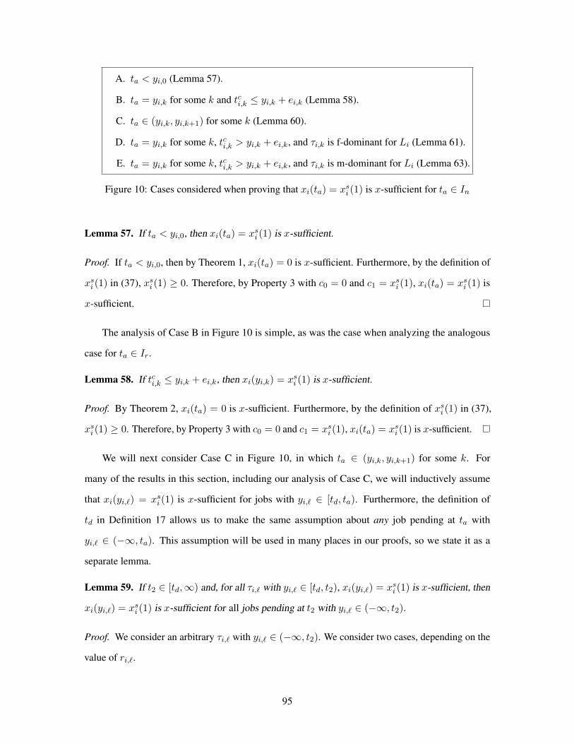
A. ta < yi,0 (Lemma 57).
B. ta = yi,k for some k and tci,k ≤ yi,k + ei,k (Lemma 58).
C. ta ∈ (yi,k, yi,k+1) for some k (Lemma 60).
D. ta = yi,k for some k, tci,k > yi,k + ei,k, and τi,k is f-dominant for Li (Lemma 61).
E. ta = yi,k for some k, tci,k > yi,k + ei,k, and τi,k is m-dominant for Li (Lemma 63).
Figure 10: Cases considered when proving that xi(ta) = xsi (1) is x-sufficient for ta ∈ In
Lemma 57. If ta < yi,0, then xi(ta) = xsi (1) is x-sufficient.
Proof. If ta < yi,0, then by Theorem 1, xi(ta) = 0 is x-sufficient. Furthermore, by the definition of
xsi (1) in (37), xsi (1) ≥ 0. Therefore, by Property 3 with c0 = 0 and c1 = xsi (1), xi(ta) = xsi (1) is
x-sufficient.
The analysis of Case B in Figure 10 is simple, as was the case when analyzing the analogous
case for ta ∈ Ir.
Lemma 58. If tci,k ≤ yi,k + ei,k, then xi(yi,k) = xsi (1) is x-sufficient.
Proof. By Theorem 2, xi(ta) = 0 is x-sufficient. Furthermore, by the definition of xsi (1) in (37),
xsi (1) ≥ 0. Therefore, by Property 3 with c0 = 0 and c1 = xsi (1), xi(ta) = xsi (1) is x-sufficient.
We will next consider Case C in Figure 10, in which ta ∈ (yi,k, yi,k+1) for some k. For
many of the results in this section, including our analysis of Case C, we will inductively assume
that xi(yi,`) = xsi (1) is x-sufficient for jobs with yi,` ∈ [td, ta). Furthermore, the definition of
td in Definition 17 allows us to make the same assumption about any job pending at ta with
yi,` ∈ (−∞, ta). This assumption will be used in many places in our proofs, so we state it as a
separate lemma.
Lemma 59. If t2 ∈ [td,∞) and, for all τi,` with yi,` ∈ [td, t2), xi(yi,`) = xsi (1) is x-sufficient, then
xi(yi,`) = xsi (1) is x-sufficient for all jobs pending at t2 with yi,` ∈ (−∞, t2).
Proof. We consider an arbitrary τi,` with yi,` ∈ (−∞, t2). We consider two cases, depending on the
value of ri,`.
95
Case 1: ri,` ∈ (−∞, td). In this case, because τi,` is pending at t2 ≥ td, τi,` is pending at td.
Therefore, the lemma follows from the definition of td in Definition 17.
Case 2: ri,` ∈ [td, t2). In this case, because yi,` ≥ ri,`, yi,` ∈ [td, t2). Thus, the lemma is true by
assumption.
We now address Case C directly.
Lemma 60. If ta ∈ [td,∞), ta ∈ (yi,k, yi,k+1) for some k, and, for all τi,` with yi,` ∈ [td, ta),
xi(yi,`) = xsi (1) is x-sufficient, then xi(ta) = xsi (1) is x-sufficient.
Proof. We consider two subcases, depending on whether τi,k is still pending at ta.
Case 1: τi,k is no longer pending at ta. In this case,
tci,k < ta
< Because xsi (1) ≥ 0 by the definition of xsi (1) in (37) and ei,k > 0
ta + xsi (1) + ei,k
By the definition of x-sufficient in Definition 8, xi(ta) = xsi (1) is x-sufficient.
Case 2: τi,k is pending at ta. By Lemma 59 with t2 = ta, xi(yi,k) = xsi (1) is x-sufficient.
Furthermore, by Theorem 3 with t = ta, xi(ta) = max0, xsi (1) − (ta − yi,k) is x-sufficient.
Additionally,
xsi (1) ≥ Because xsi (1) > 0 and ta > yi,k
max0, xsi (1)− (ta − yi,k).
Therefore, by Property 3 with c0 = max0, xsi (1)− (ta − yi,k), and c1 = xsi (1), xi(ta) = xsi (1) is
x-sufficient.
We now address Case D, in which ta = yi,k for some k and τi,k is f-dominant for Li.
Lemma 61. If ta ∈ In, ta = yi,k for some τi,k, τi,k is f-dominant for Li, and xi(yi,`) = xsi (1) is
x-sufficient for all τi,` such that yi,` ∈ [td, yi,k), then xi(ta) = xsi (1) is x-sufficient.
96
Proof. Lemma 23 describes the relationship between yi,k−1 and yi,k in virtual time. We now bound
their difference in actual time.
(yi,k − yi,k−1) ≥ By Lemma 31 with sub = 1
v(yi,k)− v(yi,k−1)
≥ By Lemma 23
v(yi,k−1) + Ti − v(yi,k−1)
= Rearranging
Ti.
Rearranging,
yi,k−1 ≤ yi,k − Ti. (107)
We have
xsi (1) = Rewriting
yi,k−1 + xsi (1) + Ci − yi,k−1 − Ci
≥ By Property 8 and the definition of f-dominant for Li in Definition 10
yi,k−1 + xsi (1) + ei,k−1 − yi,k−1 − Ci
≥ By Lemma 59, (107), and the definition of x-sufficient in Definition 8
tci,k−1 − yi,k−1 − Ci
≥ By (107)
tci,k−1 − yi,k + Ti − Ci
≥ By the choice of Li in Definition 12
tci,k−1 − yi,k +Arni (m− Li − 1)− Ci
≥ By Lemma 8
tci,k−1 − yi,k +Ai,k(m− Li − 1)− ei,k
= By the definition of xfi,k in (15)
97
xfi,k.
Furthermore, by Theorem 4, because τi,k is f-dominant for Li, xi(ta) = xi(yi,k) = xfi,k is
x-sufficient. Therefore, by Property 3 with c0 = xfi,k and c1 = xsi (1), xi(ta) = xsi (1) is x-
sufficient.
We finally consider Case E in Figure 10, in which ta = yi,k for some k and τi,k is m-dominant
for Li. We will reuse many of the lemmas from our analysis of the same case with ta ∈ Ir. However,
we will show in Lemma 62 below that in some circumstances we can use xpi (t) = xsi (1) in place of
xpi (t) = xpri (t). The proof of Lemma 62, like the proof of Lemma 30, is based on Lemma 29 that
considers xi(t) for certain values of t.
Lemma 62. Let τj be arbitrary. If t2 ∈ [td,∞) and for all τj,` such that yj,` ∈ [td, t2), xj(yj,`) =
xsj(1) is x-sufficient, then xpj (t2) = xsj(1) is xp-sufficient.
Proof. We consider an arbitrary τj,` pending at t2. We consider two cases, depending on the value of
yj,`.
Case 1: yj,` ∈ (−∞, t2). In this case, by Lemma 59 with i = j, xj(yj,`) = xsj(1) is x-sufficient.
Therefore, by Lemma 29, yj,` ≥ t2 − (xsj(1) + ecj,`(t2)).
Case 2: yj,` ∈ [t2,∞). In this case,
yj,` ≥ t2
≥ Because xsi (1) ≥ 0 by the definition of xsj(1) in (37), and because ecj,`(t2) ≥ 0
t2 − (xsj(1) + ecj,`(t2))
Because τj,` was arbitrary, the lemma holds by the definition of xp-sufficient in Definition 16.
We now provide the analysis for Case E in Figure 10.
Lemma 63. If ta = yi,k for some k, ta ∈ [td,∞), xj(yj,`) = xsj(1) is x-sufficient for all τj,` with
yj,` ∈ [td, ta), and τi,k is m-dominant for Li, then xi(ta) = xsi (1) is x-sufficient.
98
Proof. Because some processor is idle at td, by the definition of tbi,k, tbi,k ≥ td. We have
xsi (1) ≥ By the definition of xsi (1) in (37)( ∑m−1 largest
(Cj + Uvj · xsj(1)− Sj) +∑τj∈τ
Sj + (m− utot − 1)Ci +Orn
+ Li · Uvi · xsi (1)
)/utot. (108)
For simplicity, we separately consider a subset of this expression.
∑m−1 largest
(Cj + Uvj · xsj(1)− Sj) +∑τj∈τ
Sj − Ci
= Rewriting∑m−1 largest
(Cj + Uvj · xsj(1)− Sj) +∑τj∈τ
Sj +∑τj∈τ
Uvj · (v(yi,k)− v(tbi,k))
−∑τj∈τ
Uvj · (v(yi,k)− v(tbi,k)) + ei,k − Ci − ei,k
≥ By Lemma 43 with sub = 1 and by Lemma 62
Wi,k −∑τj∈τ
Uvj · (v(yi,k)− v(tbi,k))− ei,k
≥ By Property 11
Wi,k − utot · (v(yi,k)− v(tbi,k))− ei,k
≥ By Lemma 31 with sub = 1
Wi,k − utot · (yi,k − tbi,k)− ei,k
= By the definition of Ri,k in (20)
Wi,k −Ri,k − ei,k. (109)
Putting it all together,
xsi (1) ≥ By (108) and (109)
Wi,k −Ri,k + (m− utot)Ci − ei,k +Orn + Li · Uvi · xsi (1)
utot
≥ By Lemma 33 with sub = 1 and Lemma 62
99
Wi,k −Ri,k + (m− utot)Ci − ei,k +Orn + Li · epi,kutot
≥ By Property 8, because tci,k > yi,k ≥ tbi,k > tr
Wi,k −Ri,k + (m− utot − 1)ei,k +Orn + Li · epi,kutot
≥ By Lemma 45
Wi,k −Ri,k + (m− utot − 1)ei,k +Oi,k + Li · epi,kutot
= By the definition of xmi,k in (23)
xmi,k. (110)
Because τi,k is m-dominant for Li, by Theorem 5, xi(ta) = xmi,k is x-sufficient. Thus, by
Property 3 with c0 = xmi,k and c1 = xsi (1), xi(ta) = xsi (1) is x-sufficient.
We finally combine the lemmas previously proved in this subsection to show that xi(ta) = xsi (1)
is x-sufficient for arbitrary ta ∈ In.
Theorem 7. For arbitrary ta ∈ In, xi(ta) = xsi (1) is x-sufficient.
Proof. The lemmas referenced in Figure 9 exhaustively consider all possible cases for ta. Further-
more, for each lemma requires that xi(t0) = xsi (1) is x-sufficient for some t0, the considered t0
is yj,` for some τj,` with yj,` ∈ [td, ta). Therefore, the x-sufficiency of xi(ta) = xsi (1) follows by
strong induction over all times t0 such that t0 = yj,` for some τj,` and yj,` ∈ [td, ta) or t0 = ta.
100
BIBLIOGRAPHY
References
Baruah, S., Koren, G., Mishra, B., Raghunathan, A., Rosier, L., and Shasha, D. (1991). On-linescheduling in the presence of overload. In Proceedings of the 32nd Annual Symposium OnFoundations of Computer Science, pages 100–110.
Beccari, G., Caselli, S., Reggiani, M., and Zanichelli, F. (1999). Rate modulation of soft real-timetasks in autonomous robot control systems. In Proceedings of the 11th Euromicro Conferenceon Real-Time Systems, pages 21–28.
Block, A. (2008). Adaptive Multiprocessor Real-Time Systems. PhD thesis, The University of NorthCarolina at Chapel Hill.
Burns, A. and Davis, R. (2013). Mixed criticality systems - a review. http://www-users.cs.york.ac.uk/˜burns/review.pdf.
Buttazzo, G. and Stankovic, J. (1993). RED: Robust earliest deadline scheduling. In Proceedings ofthe 3rd International Workshop on Responsive Computing Systems, pages 100–111.
Chakraborty, S., Kunzli, S., and Thiele, L. (2003). A general framework for analysing systemproperties in platform-based embedded system designs. In Proceedings of the 2003 Design,Automation and Test in Europe Conference and Exhibition, pages 190–195.
Erickson, J. P., Anderson, J. H., and Ward, B. C. (2014). Fair lateness scheduling: reducing maximumlateness in G-EDF-like scheduling. Real-Time Systems, 50(1):5–47.
Garyali, P. (2010). On best-effort utility accrual real-time scheduling on multiprocessors. Master’sthesis, The Virginia Polytechnic Institute and State University.
Herman, J., Kenna, C., Mollison, M., Anderson, J., and Johnson, D. (2012). Rtos support formulticore mixed-criticality systems. In Proceedings of the 18th IEEE Real-Time and EmbeddedTechnology and Applications Symposium, pages 197–208.
Jan, M., Zaourar, L., and Pitel, M. (2013). Maximizing the execution rate of low-criticality tasks inmixed criticality systems. In Proceedings of the 1st Workshop on Mixed Criticality Systems,pages 43–48.
Koren, G. and Shasha, D. (1992). dover: an optimal on-line scheduling algorithm for overloadedreal-time systems. In Proceedings of the 13th Real-Time Systems Symposium, pages 290–299.
Leontyev, H. and Anderson, J. H. (2010). Generalized tardiness bounds for global multiprocessorscheduling. Real-Time Systems, 44(1-3):26–71.
Leontyev, H., Chakraborty, S., and Anderson, J. H. (2011). Multiprocessor extensions to real-timecalculus. Real-Time Systems, 47(6):562–617.
Locke, C. (1986). Best-Effort Decision Making for Real-Time Scheduling. PhD thesis, CarnegieMellon University.
101
Mollison, M. S., Erickson, J. P., Anderson, J. H., Baruah, S. K., and Scoredos, J. A. (2010). Mixed-criticality real-time scheduling for multicore systems. In Proceedings of the IEEE InternationalConference on Embedded Software and Systems, pages 1864–1871, Washington, DC, USA.IEEE Computer Society.
Santy, F., George, L., Thierry, P., and Goossens, J. (2012). Relaxing mixed-criticality schedulingstrictness for task sets scheduled with fp. In Proceedings of the 24th Euromicro Conference onReal-Time Systems, pages 155–165.
Santy, F., Raravi, G., Nelissen, G., Nelis, V., Kumar, P., Goossens, J., and Tovar, E. (2013). Two pro-tocols to reduce the criticality level of multiprocessor mixed-criticality systems. In Proceedingsof the 21st International Conference on Real-Time Networks and Systems, pages 183–192, NewYork, NY, USA. ACM.
Stoica, I., Abdel-Wahab, H., Jeffay, K., Baruah, S., Gehrke, J., and Plaxton, C. (1996). A proportionalshare resource allocation algorithm for real-time, time-shared systems. In Proceedings of the17th IEEE Real-Time Systems Symposium, pages 288–299.
Su, H. and Zhu, D. (2013). An elastic mixed-criticality task model and its scheduling algorithm. InProceedings of the 2013 Design, Automation Test in Europe Conference Exhibition (DATE),pages 147–152.
Su, H., Zhu, D., and Mosse, D. (2013). Scheduling algorithms for elastic mixed-criticality tasks inmulticore systems. In Proceedings of the 19th IEEE International Conference on Embeddedand Real-Time Computing Systems and Applications, pages 352–357.
Zhang, L. (1990). Virtual clock: A new traffic control algorithm for packet switching networks. InProceedings of the 5th ACM Symposium on Communications Architectures & Protocols, pages19–29, New York, NY, USA. ACM.
102
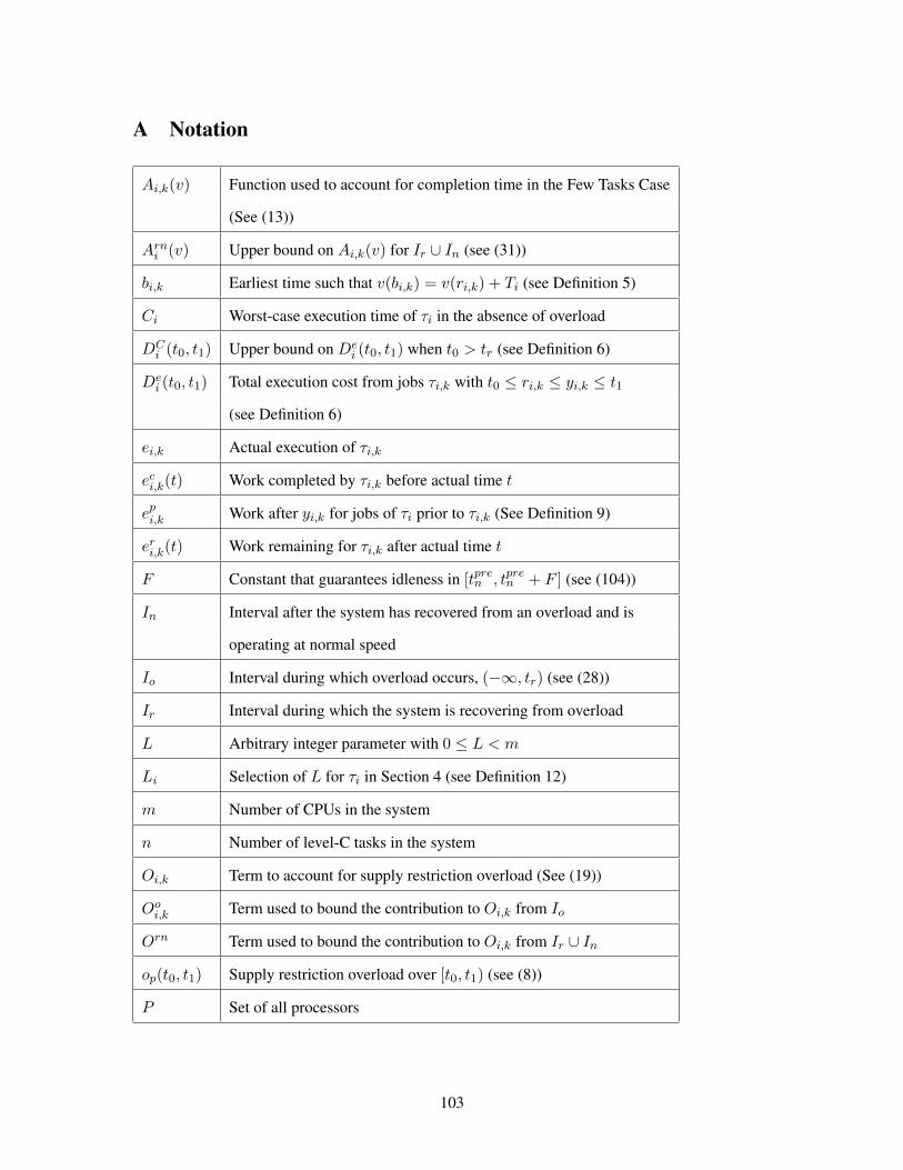
A Notation
Ai,k(v) Function used to account for completion time in the Few Tasks Case
(See (13))
Arni (v) Upper bound on Ai,k(v) for Ir ∪ In (see (31))
bi,k Earliest time such that v(bi,k) = v(ri,k) + Ti (see Definition 5)
Ci Worst-case execution time of τi in the absence of overload
DCi (t0, t1) Upper bound on De
i (t0, t1) when t0 > tr (see Definition 6)
Dei (t0, t1) Total execution cost from jobs τi,k with t0 ≤ ri,k ≤ yi,k ≤ t1
(see Definition 6)
ei,k Actual execution of τi,k
eci,k(t) Work completed by τi,k before actual time t
epi,k Work after yi,k for jobs of τi prior to τi,k (See Definition 9)
eri,k(t) Work remaining for τi,k after actual time t
F Constant that guarantees idleness in [tpren , tpren + F ] (see (104))
In Interval after the system has recovered from an overload and is
operating at normal speed
Io Interval during which overload occurs, (−∞, tr) (see (28))
Ir Interval during which the system is recovering from overload
L Arbitrary integer parameter with 0 ≤ L < m
Li Selection of L for τi in Section 4 (see Definition 12)
m Number of CPUs in the system
n Number of level-C tasks in the system
Oi,k Term to account for supply restriction overload (See (19))
Ooi,k Term used to bound the contribution to Oi,k from Io
Orn Term used to bound the contribution to Oi,k from Ir ∪ In
op(t0, t1) Supply restriction overload over [t0, t1) (see (8))
P Set of all processors
103
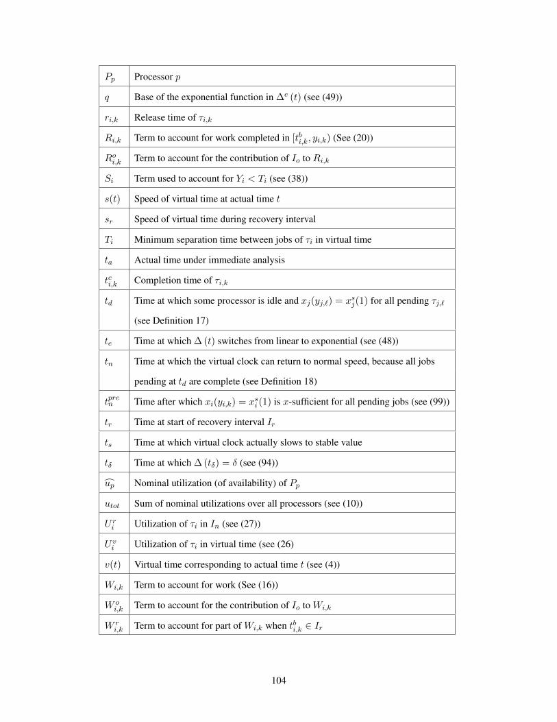
Pp Processor p
q Base of the exponential function in ∆e (t) (see (49))
ri,k Release time of τi,k
Ri,k Term to account for work completed in [tbi,k, yi,k) (See (20))
Roi,k Term to account for the contribution of Io to Ri,k
Si Term used to account for Yi < Ti (see (38))
s(t) Speed of virtual time at actual time t
sr Speed of virtual time during recovery interval
Ti Minimum separation time between jobs of τi in virtual time
ta Actual time under immediate analysis
tci,k Completion time of τi,k
td Time at which some processor is idle and xj(yj,`) = xsj(1) for all pending τj,`
(see Definition 17)
te Time at which ∆ (t) switches from linear to exponential (see (48))
tn Time at which the virtual clock can return to normal speed, because all jobs
pending at td are complete (see Definition 18)
tpren Time after which xi(yi,k) = xsi (1) is x-sufficient for all pending jobs (see (99))
tr Time at start of recovery interval Ir
ts Time at which virtual clock actually slows to stable value
tδ Time at which ∆ (tδ) = δ (see (94))
up Nominal utilization (of availability) of Pp
utot Sum of nominal utilizations over all processors (see (10))
U ri Utilization of τi in In (see (27))
Uvi Utilization of τi in virtual time (see (26)
v(t) Virtual time corresponding to actual time t (see (4))
Wi,k Term to account for work (See (16))
W oi,k Term to account for the contribution of Io to Wi,k
W ri,k Term to account for part of Wi,k when tbi,k ∈ Ir
104
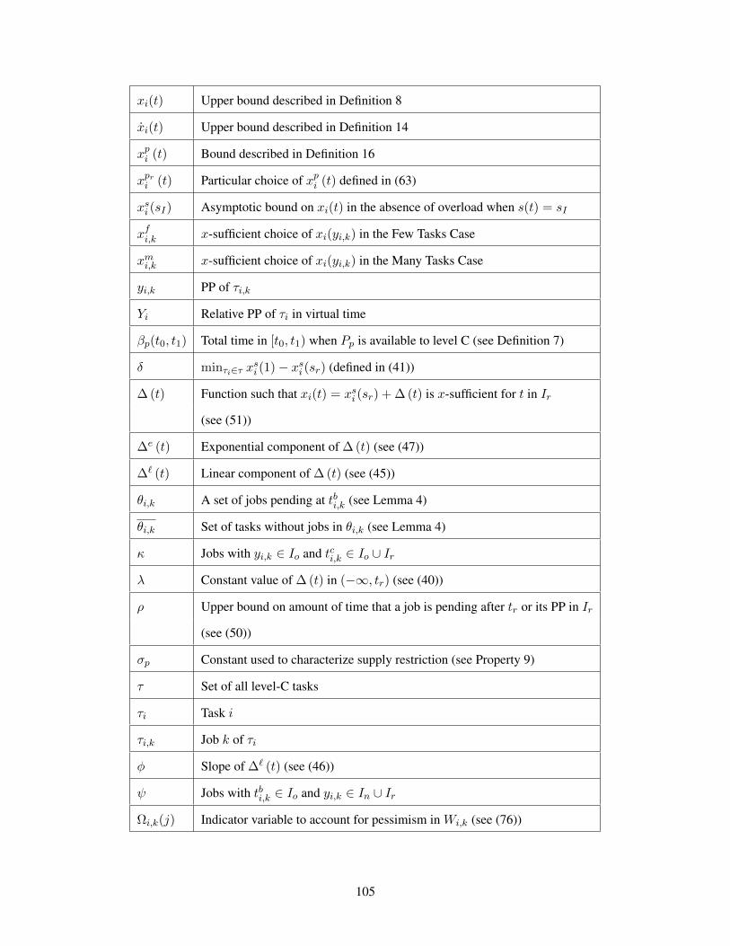
xi(t) Upper bound described in Definition 8
xi(t) Upper bound described in Definition 14
xpi (t) Bound described in Definition 16
xpri (t) Particular choice of xpi (t) defined in (63)
xsi (sI) Asymptotic bound on xi(t) in the absence of overload when s(t) = sI
xfi,k x-sufficient choice of xi(yi,k) in the Few Tasks Case
xmi,k x-sufficient choice of xi(yi,k) in the Many Tasks Case
yi,k PP of τi,k
Yi Relative PP of τi in virtual time
βp(t0, t1) Total time in [t0, t1) when Pp is available to level C (see Definition 7)
δ minτi∈τ xsi (1)− xsi (sr) (defined in (41))
∆ (t) Function such that xi(t) = xsi (sr) + ∆ (t) is x-sufficient for t in Ir
(see (51))
∆e (t) Exponential component of ∆ (t) (see (47))
∆` (t) Linear component of ∆ (t) (see (45))
θi,k A set of jobs pending at tbi,k (see Lemma 4)
θi,k Set of tasks without jobs in θi,k (see Lemma 4)
κ Jobs with yi,k ∈ Io and tci,k ∈ Io ∪ Ir
λ Constant value of ∆ (t) in (−∞, tr) (see (40))
ρ Upper bound on amount of time that a job is pending after tr or its PP in Ir
(see (50))
σp Constant used to characterize supply restriction (see Property 9)
τ Set of all level-C tasks
τi Task i
τi,k Job k of τi
φ Slope of ∆` (t) (see (46))
ψ Jobs with tbi,k ∈ Io and yi,k ∈ In ∪ Ir
Ωi,k(j) Indicator variable to account for pessimism in Wi,k (see (76))
105
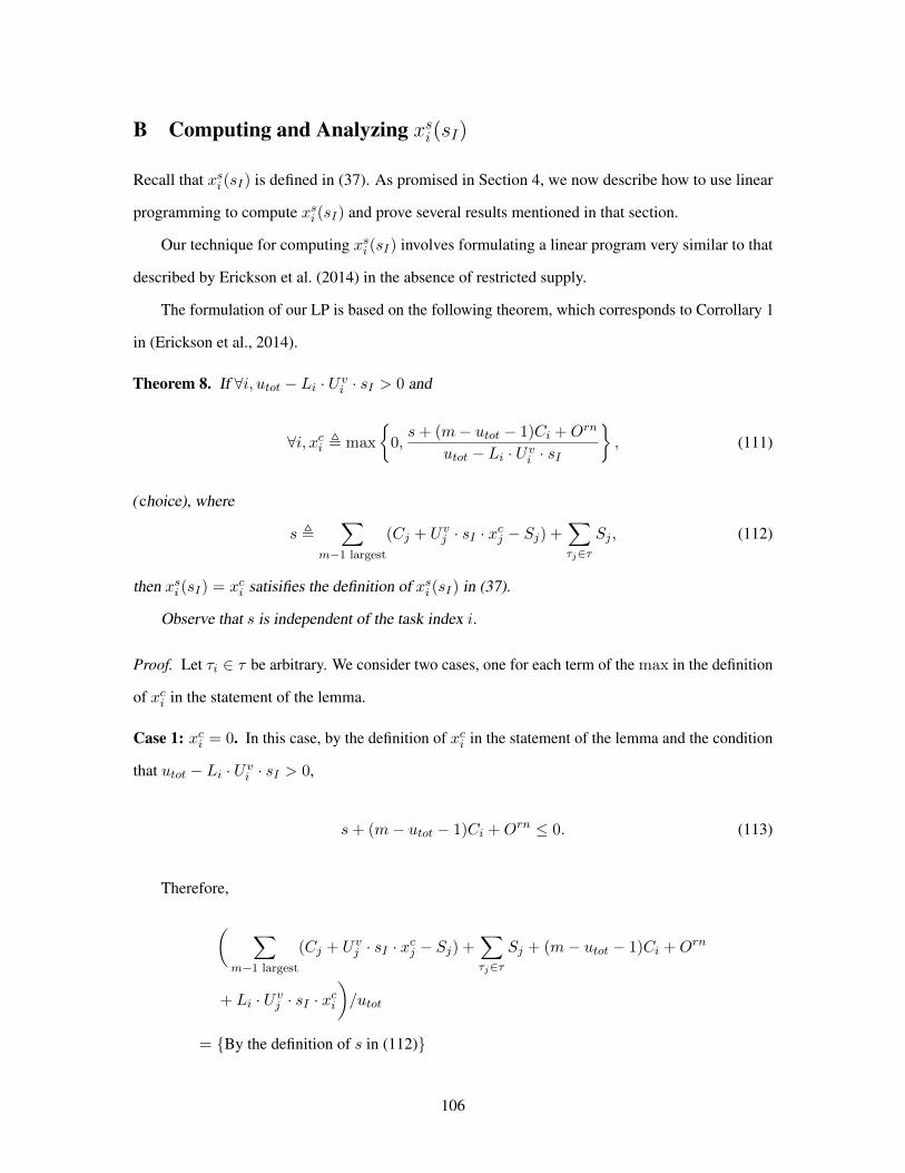
B Computing and Analyzing xsi (sI)
Recall that xsi (sI) is defined in (37). As promised in Section 4, we now describe how to use linear
programming to compute xsi (sI) and prove several results mentioned in that section.
Our technique for computing xsi (sI) involves formulating a linear program very similar to that
described by Erickson et al. (2014) in the absence of restricted supply.
The formulation of our LP is based on the following theorem, which corresponds to Corrollary 1
in (Erickson et al., 2014).
Theorem 8. If ∀i, utot − Li · Uvi · sI > 0 and
∀i, xci , max
0,s+ (m− utot − 1)Ci +Orn
utot − Li · Uvi · sI
, (111)
(choice), where
s ,∑
m−1 largest
(Cj + Uvj · sI · xcj − Sj) +∑τj∈τ
Sj , (112)
then xsi (sI) = xci satisifies the definition of xsi (sI) in (37).
Observe that s is independent of the task index i.
Proof. Let τi ∈ τ be arbitrary. We consider two cases, one for each term of the max in the definition
of xci in the statement of the lemma.
Case 1: xci = 0. In this case, by the definition of xci in the statement of the lemma and the condition
that utot − Li · Uvi · sI > 0,
s+ (m− utot − 1)Ci +Orn ≤ 0. (113)
Therefore,
( ∑m−1 largest
(Cj + Uvj · sI · xcj − Sj) +∑τj∈τ
Sj + (m− utot − 1)Ci +Orn
+ Li · Uvj · sI · xci)/utot
= By the definition of s in (112)
106
s+ (m− utot − 1)Ci +Orn + Li · Uvi · sI · xciutot
= By the case we are considering
s+ (m− utot − 1)Ci +Orn
utot
≤ By (113)
0.
Thus, xsi (sI) = xci satisfies the definition of xsi (sI) in (37) for τi.
Case 2: xci > 0. In this case, by the definition of xci in the statement of the lemma we have
xci =s+ (m− utot − 1)Ci +Orn
utot − Li · Uvi · sI.
We manipulate this expression to the form in the definition of xsi (sI) in (37). Multiplying both sides
by utot−Li·Uvi ·sIutot
yields
utot − Li · Uvi · sIutot
· xci =s+ (m− utot − 1)Ci +Orn
utot.
Adding Li·Uvi ·sIutot
· xci to both sides yields
xci =s+ (m− utot − 1)Ci +Orn + Li · Uvi · sI · xci
utot.
Finally, substituting the expression for s in (112),
xci =
( ∑m−1 largest
(Cj + Uvj · sI · xcj − Sj) +∑τj∈τ
Sj + (m− utot − 1)Ci +Orn
+ Li · Uvi · sI · xci)/utot.
By the case we are considering, both sides of this expression must be greater than zero. Thus,
xsi (sI) = xci satisfies the definition of xsi (sI) in (37) for τi.
Our LP has, for each τi, a variable xci as in Theorem 8, corresponding to xsi (sI) and an auxilliary
variable zi. Our LP also has task-independent variables s (as in Theorem 8), G (corresponding to the
107
first sum in the definition of s in (112)), Ssum (corresponding to the second sum in the definition of s
in (112)) and auxilliary variable b. All other quantities that appear are constants.
We will present constraint sets for determining xci in the same order as the constraint sets in
Section 4 in (Erickson et al., 2014). The first constraint set ensures that
xci ≥ max
0,s+ (m− utot − 1)Ci +Orn
utot − Li · Uvi · sI
. (114)
It corresponds to Constraint Set 1 in Erickson et al. (2014) that defined xi, but provides only an
inequality. Although Theorem 8 requires equality, this discrepancy will be handled in Lemma 66
below.
Constraint Set 1.
∀i : xci ≥s+ (m− utot − 1) · Ci +Orn
utot − Li · Uvi · sI,
∀i : xci ≥ 0.
Because we consider Si to be a constant, we do not require a constraint that corresponds with
Constraint Set 2 in (Erickson et al., 2014).
The next constraint set is used to determine the value of the first sum in the definition of s in
(112). This sum corresponds with G(~x, ~Y ) in (Erickson et al., 2014), so the constraint is almost
identical to Constraint Set 3 in (Erickson et al., 2014). As discussed there, this constraint actually
ensures that G provides an upper bound on that sum, rather than an exact value. In other words, it
actually guarantees that
G ≥∑
m−1 largest
(Ci + Uvi · sI · xci − Si). (115)
Although Theorem 8 requires equality, this discrepancy will be handled in Lemma 65 below.
Constraint Set 2.
G = b(m− 1) +∑τi∈τ
zi,
∀i : zi ≥ 0,
108
zi ≥ Ci + Uvi · sI · xci − Si − b.
Rather than having a constraint that corresponds to Constraint Set 4 in (Erickson et al., 2014),
we define a constant
Ssum =∑τj∈τ
Sj . (116)
The next constraint provides a bound on the value of s. This constraint differs from the definition
of s in (112) because it is an inequality. However, we will show in Lemma 65 below that for an
optimal solution to the LP, it reduces to an equality. This constraint corresponds to Constraint Set 5
in (Erickson et al., 2014).
Constraint Set 3.
s ≥ G+ Ssum.
We must show that, for some appropriate optimization function, an optimal solution to Constraint
Sets 1–3 can be used to compute the values of s and xci described in Theorem 8. We will show below
that if we minimize s and an optimal solution is found, we can use the resulting s in the definition of
xci in (111), and (112) must be satisfied as well with that choice of xci .
To do so, we first characterize the value of s for any feasible solution, providing a lower bound
in Lemma 64 and a characterization relating to an optimal value in Lemma 65. Observe that the
expression in Lemma 64 is identical to the definition of s in (112), except that it replaces the equality
with an inequality.
Lemma 64. For any feasible assignment of variables satisfying Constraint Sets 1–3,
s ≥∑
m−1 largest
(Ci + Uvi · sI · xci − Si) +∑τj∈τ
Si.
Proof. We have
s ≥ By Constraint Set 3
G+ Ssum
≥ By (115)
109
∑m−1 largest
(Cj + Uvj · sI · xcj − Sj) + Ssum
= By the definition of Ssum in (116)∑m−1 largest
(Cj + Uvj · sI · xcj − Sj) +∑τj∈τ
Sj .
The next lemma will be used to characterize the optimal value of s with an appropriate optimiza-
tion function.
Lemma 65. If V is a feasible assignment of variables that satisfies Constraint Sets 1–3 and
s >∑
m−1 largest
(Cj + Uvj · sI · xcj − Sj) +∑τj∈τ
Si,
then there is also a feasible assignment of variables V ′ (with variable assignments denoted with
primes) such that s > s′. In other words, s has not taken its optimal value upon minimization.
Proof. We use the following assignment for V ′:
s′ =∑
m−1 largest
(Cj + Uvj · sI · xcj − Sj) + Ssum, (117)
∀i, xc′i = xci , (118)
G′ =∑
m−1 largest
(Cj + Uvj · sI · xcj − Sj), (119)
b′ = (m− 1)th largest value of Cj + Uvj · sI · xcj − Sj , (120)
∀i, z′i = max0, Cj + Uvj · sI · xcj − Sj − b′. (121)
By the statement of the lemma, the definition of Ssum in (116), and by (117),
s > s′. (122)
110
We will first show that Constraint Set 1 holds by considering arbitrary τi.
xc′i = By (118)
xci
≥ By (114)
max
0,s+ (m− utot − 1)Ci +Orn
utot − Li · Uvi · sI
≥ By (122)
max
0,s′ + (m− utot − 1)Ci +Orn
utot − Li · Uvi · sI
. (123)
Constraint Set 2 holds by (118)–(121).
To show Constraint Set 3 holds,
s′ = By (117)∑m−1 largest
(Cj + Uvj · sI · xcj − Sj) + Ssum
= By (119)
G+ Ssum.
By Lemmas 64–66, we can minimize s as our optimization objective, and the definition of s in
Theorem 8 must be satisfied by the resulting solution. However, the definition of xci in (111) is not
guaranteed to hold, because Constraint Set 1 also guaranteed only an inequality. Fortunately, we
can use the resulting value of s in (111) to compute correct values of xci , as shown in the following
lemma.
Lemma 66. If V is a feasible assignment of variables satisfying Constraint Sets 1–3, then there
is also an assignment V ′ (with variables denoted with primes, as before) such that s′ = s and
∀i, xci = max
0, s+(m−utot−1)Ci+Orn
utot−Li·Uvi ·sI
.
111
Proof. We use the following assignment for V ′:
s′ = s, (124)
∀i, xc′i = max
0,s+ (m− utot − 1)Ci +Orn
utot − Li · Uvi · sI
, (125)
G′ =∑
m−1 largest
(Cj + Uvj · sI · xc′j − Sj), (126)
b′ = (m− 1)th largest value of Cj + Uvj · sI · xc′j − Sj , (127)
∀i, z′i = max0, Cj + Uvj · sI · xc′j − Sj − b′. (128)
Constraint Set 1 holds by (125).
Constraint Set 2 holds by (126)–(128).
To show that Constraint Set 3 holds, we first show that for arbitrary j,
xcj ≥ By (114)
max
0,s+ (m− utot − 1)Cj +Orn
utot − Lj · Uvj · sI
= By (125)
xc′j . (129)
Then, we have
s′ = By (124)
s
≥ By Lemma 64∑m−1 largest
(Cj + Uvj · sI · xcj − Sj) +∑τj∈τ
Sj
≥ By (129)∑m−1 largest
(Cj + Uvj · sI · xc′j − Sj) +∑τj∈τ
Sj
= By (126)
112
G′ +∑τj∈τ
Sj
= By the definition of Ssum in (116)
G′ + Ssum.
We will next show that, if Property 10 holds, a minimum feasible s does in fact exist. While
proving this result, we will several times exploit the fact that Sj is nonnegative, as shown now.
Lemma 67. For all j, Sj ≥ 0.
Proof. We have
Sj = By the definition of Sj in (38)
Cj ·(
1− YiTi
)≥ Because Yi ≤ Ti
Cj ·(
1− TjTj
)= Cancelling
0.
We now show that a lower bound on s exists for feasible assignments. We will later show that
feasible assignments do exist. Together, these results are sufficient to show that an optimal value of s
exists.
Lemma 68. For any feasible assignment of variables V satisfying Constraint Sets 1–3,
s ≥∑
m−1 largest
Ci.
113
Proof. Now, we show that
s ≥ By Lemma 64∑m−1 largest
(Cj + Uvj · sI · xci − Sj) +∑τj∈τ
Sj
≥ By Lemma 67; observe that each Sj appearing in the first summation
also appears in the second∑m−1 largest
(Cj + Uvj · sI · xci )
≥ By Constraint Set 1∑m−1 largest
Cj .
We now show that, given Property 10, the LP is feasible.
Lemma 69. If Property 10 holds, then a feasible assignment of variables V for Constraint Sets 1–3
exists.
Proof. Let Cmax be the largest Ci in the system. For notational convenience, let
Usum ,∑
m−1 largest
Uvj , (130)
Ltmax , maxτj∈τ
LjUvj (131)
(term). We use the following assignment for V :
s = max
Cmax,
Usum · (mCmax +Orn) + (utot − Ltmax) · ((m− 1)Cmax + Ssum)
utot − Ltmax − Usum
,
(132)
∀i, xci =s+ (m− utot − 1)Ci +Orn
utot − Li · Uvi · sI, (133)
G =∑
m−1 largest
(Cj + Uvj · sI · xcj − Sj), (134)
114
b = (m− 1)th largest value of Cj + Uvj · sI · xcj − Sj , (135)
∀i, zi = max0, Cj + Uvj · sI · xcj − Sj − b. (136)
To demonstrate that Constraint Set 1 holds, we first bound the expression that appears in the
denominator of the definition of xci in (133).
utot − Lj · Uvj · sI ≥ Because sI ≤ 1
utot − Lj · Uvj
≥ By the definition of “max”
utot −maxτj∈τ
Lj · Uvj
> By Property 10∑m−1 largest
Uvj
≥ Because each Uvj > 0
0. (137)
The first constraints in Constraint Set 1 hold by (133). We now show that the second constraint also
holds.
xci = By (133)
s+ (m− utot − 1)Ci +Orn
utot − Li · Uvi · sI
≥ By (132) and (137)
Cmax + (m− utot − 1)Ci +Orn
Li · Uvi · sI
≥ By the definition of Cmax and by (137)
(m− utot)Ci +Orn
Li · Uvi · sI
≥ By (137), because Ci and Orn are nonnegative
0. (138)
115
Constraint Set 2 holds by (134)–(136).
By (132),
s ≥ Usum · (mCmax +Orn) + (utot − Ltmax) · ((m− 1)Cmax + Ssum)
utot − Ltmax − Usum. (139)
To show that Constraint Set 3 holds, we start by multiplying both sides of (139) by utot−Ltmax−Usum
utot−Ltmax,
resulting in
utot − Ltmax − Usum
utot − Ltmax
· s ≥ Usum · (mCmax +Orn)
utot − Ltmax
+ (m− 1)Cmax + Ssum.
Adding Usumutot−Ltmax
· s to both sides yields
s ≥ Usum · (s+mCmax +Orn)
utot − Ltmax
+ (m− 1)Cmax + Ssum. (140)
Thus, we have
s ≥ Rewriting (140)∑m−1 largest
(Cmax + Uvj ·
s+mCmax +Orn
utot − Ltmax
)+ Ssum
≥ By the definition of Ltmax in (131), and because sI ≤ 1∑m−1 largest
(Cmax + Uvj ·
s+mCmax +Orn
utot − Lj · Uvj · sI
)+ Ssum
≥ By (137) and the definition of Cmax∑m−1 largest
(Cj + Uvj ·
s+mCj +Orn
utot − Lj · Uvj · sI
)+ Ssum
≥ Because Cj > 0 and by (137)∑m−1 largest
(Cj + Uvj ·
s+ (m− utot − 1)Cj +Orn
utot − Lj · Uvj · sI
)+ Ssum
= By (133)∑m−1 largest
(Cj + Uvj · xci
)+ Ssum
116
≥ Because 0 < sI ≤ 1 and by (138)∑m−1 largest
(Cj + Uvj · sI · xci
)+ Ssum
≥ By Lemma 67∑m−1 largest
(Cj + Uvj · sI · xci − Sj
)+ Ssum
= By (134)
G+ Ssum..
The one promised result that remains to be shown is that a feasible solution exists for any s′I ≤ 1
as long as one exists for sI = 1. We show that result now.
Lemma 70. If a feasible assignment of variables V satisfies Constraint Sets 1–3 with sI = 1 and
utot − Li · Uvi > 0, then a feasible assignment of variables V ′ satisfies Constraint Sets 1–3 for
arbitary s′I ≤ 1.
Proof. We use the following assignment for V ′:
s′ = s, (141)
∀i, xc′i = xci , (142)
G′ =∑
m−1 largest
(Cj + Uvj · s′I · xcj − Sj), (143)
b′ = (m− 1)th largest value of Cj + Uvj · s′I · xcj − Sj , (144)
∀i, z′i = max0, Cj + Uvj · s′I · xcj − Sj − b′. (145)
Because utot − Li · Uvi > 0 and 0 < sI ≤ 1,
utot − Li · sI · Uvi > 0. (146)
To show that Constraint Set 1 holds, we consider two cases for each τi.
117
Case 1: s+ (m− utot − 1)Ci +Orn ≤ 0. In this case,
xc′i = By (142)
xci
≥ By Constraint Set 1
0
= By (146) and the case we are considering
max
0,s+ (m− utot − 1)Ci +Orn
utot − Li · sI · Uvi
.
Case 2: s+ (m− utot − 1)Ci +Oi,k > 0. In this case,
xc′i = By (142)
xci
≥ By (114) with sI = 1
max
0,s+ (m− utot − 1)Ci +Orn
utot − Li · Uvi
= By (141)
max
0,s′ + (m− utot − 1)Ci +Orn
utot − Li · Uvi
≥ By (146) and the case we are considering, because 0 < sI < 1
max
0,s′ + (m− utot − 1)Ci +Orn
utot − Li · sI · Uvi
.
Constraint Set 2 holds by (142) and (119)–(145).
To show Constraint Set 3 holds,
s′ = By (141)
s
≥ By Lemma 64 with sI = 1∑m−1 largest
(Cj + Uvj · xcj − Sj) + Ssum
118
≥ Because 0 < s′I ≤ 1∑m−1 largest
(Cj + Uvj · s′I · xcj − Sj) + Ssum
= By (142) and (143)
G+ Ssum.
Finally, we briefly discuss the use of LP to determine a choice of Yi. The value of Yi in our
analysis is assumed to remain constant when the virtual clock speed changes. Furthermore, during
the typical behavior of a system, sI = 1 should be used. Therefore, if using linear programming to
determine the best choice of Yi, it should be done using sI = 1.
Up to this point, Yi has been assumed to be a constant. Similarly, Si, which depends on Yi by
the definition of Si in (38), and Ssum, which depends on Si by the definition of Ssum in (116), have
also been considered to be constants. These can be changed to variables as long as the following
constraint sets are added. The first constrains the choice of Yi itself to match the assumptions used in
our analysis.
Constraint Set 4.
∀i, Yi ≥ 0,
∀i, Ti ≥ Yi.
The next constraint set simply specifies the value of Si according to the definition of Si in (38).
Constraint Set 5.
∀i, Si = Ci ·(
1− YiTi
).
The final constraint set specifies the value of Ssum according to the definition of Ssum in (116).
Constraint Set 6.
Ssum =∑τj∈τ
Sj .
119
Any optimization function can be used that ensures, under an optimal solution, the minimal
value of s with respect to the chosen values of Yi. If the optimization function has such a property,
then all of the reasoning in this appendix will continue to hold. Because each xci cannot increase as a
result of an increase in s, such a property is easy to achieve for a reasonable optimization function.
120