Discussion Paper Series A No.446

The Big Mac Standard: A Statistical Illustration

Hiroshi Fujiki (Institute for Monetary and Economic Studies, Bank of Japan)

and Yukinobu Kitamura

(The Institute of Economic Research, Hitotsubashi University)

November 2003

The Institute of Economic Research Hitotsubashi University

Kunitachi, Tokyo, 186-8603 Japan

Corresponding author: Yukinobu Kitamura, Institute of Economic Research, Hitotsubashi University, 2-1 Naka, Kunitachi City, Tokyo 186-8603, Japan. E-mail: kitamura@ier.hit-u.ac.jp. Telephone: 042-580-8394. Fax Number: 042-580-8394. We thank Akira Kohsaka for his useful comments on an earlier version of this paper. Any views expressed in this paper are solely those of the authors’, and do not represent the view of the Bank of Japan.

The Big Mac Standard: A Statistical Illustration

Hiroshi FUJIKI Institute for Monetary and Economic Studies

Bank of Japan

Yukinobu KITAMURA Institute of Economic Research

Hitotsubashi University

First Draft: March, 1997 Second Draft: September, 2002

Revised: October, 2003

Abstract

We demonstrate a statistical procedure for selecting the most suitable empirical

model to test an economic theory, using the example of the test for purchasing

power parity based on the Big Mac Index. Our results show that supporting

evidence for purchasing power parity, conditional on the Balassa–Samuelson effect,

depends crucially on the selection of models, sample periods and economies used

for estimations.

Key Words: Big Mac Index, Purchasing Power Parity, Panel Data

JEL Classification: F31, C23

1

1．Introduction

The well-known law of one price, one of the strongest versions of purchasing power parity

(PPP), requires, for any tradable goods i, p Epi i= * , where pi is the nominal price of good i

in the domestic currency, E is the domestic price of foreign currency, and pi* is the nominal

price of good i in foreign currency.

Following Nelson (2001), we briefly summarize the empirical literature testing

purchasing power parity using time series macroeconomic data.

Before the 1980s, researchers testing purchasing power parity usually estimated

equation (1) and tested the joint hypothesis of α β= =0 1, ,

ln( ) [ln( ) ln( )]*E P Pt t t t= + ⋅ − +α β ε , (1)

where Et is the nominal exchange rate, Pt is the domestic price index, Pt* is the foreign

price index, ε t is an error term, and subscript t indicates time t.

Since Dickey and Fuller (1979, 1981) proposed formal tests for the existence of a unit

root, it has been reported that most macroeconomic time series, including nominal exchange

rate and price level, had a unit root. Given recent developments econometric analysis of

non-stationary data, a test for purchasing power parity typically tests whether the real

exchange rate, or q E P Pt t t t= − +ln( ) ln( ) ln( )* , is stationary or not. A major problem in

such lines of research is that the test for purchasing power parity requires a very long run of

data to reject the null hypothesis of the existence of a unit root. Thus, recently, economists

have emphasized the use of unit root tests that apply to panel data (see for an earlier example,

Wu, 1993).

According to Nelson (2001), such studies find that purchasing power parity tends to

hold if researchers use long-run time series data. In addition, the half-life of the deviation

from purchasing power parity is, on average, 3.7 years when one uses quarterly CPI data and

the nominal exchange rate relative to the US dollar (Nelson, 2001, Table 7.2). One of the

most promising reasons for such deviations from purchasing power parity is the Balassa–

Samuelson effect (Balassa, 1963; Samuelson, 1964). The other hypothesis is that the firm's

response to changes in nominal prices does not follow immediately if shocks in the nominal

exchange rate are perceived to be temporary.

2

Most empirical studies on purchasing power parity have employed aggregated data,

since it is not easy to design a common basket of commodities to make consistent cross-

country comparison of nominal price levels. In this context, the annual publication of the

Big Mac Index by The Economist is a notable exception. Essentially, the Big Mac PPP is

the exchange rate that would mean hamburgers cost the same in the US as abroad. Namely,

the Big Mac Index tests whether the relative prices of an identical basket of goods and

services measured by a McDonald's Big Mac, in terms of domestic currencies, is equal to

nominal exchange rates in the financial markets in the long run. This is possible because the

Big Mac is produced in about 120 countries.

There are several studies using this Index. For example, Pakko and Pollard (1996)

admit that the Big Mac Index is useful for testing purchasing power parity. However, they

conclude that purchasing power parity does not hold for the following reasons: barriers to

trade, the inclusion of non-traded goods in the Big Mac, imperfect competition in goods

markets and factor markets, and current account imbalances. On the other hand, Ong (1997)

reports that the Big Max Index is surprisingly accurate in tracking exchange rates over the

long-term. Click (1996) also finds that purchasing power parity based on the Big Mac Index

holds in the time-series dimensions, and that the country-specific deviations from purchasing

power parity are explained by the Balassa–Samuelson effect.

In this paper, we show that the results for the acceptance or rejection of purchasing

power parity using the Big Max Index are sensitive to the choice of statistical models, and

thus it might be desirable to employ various statistical techniques. This result is based not

only on statistical tests, but also on the properties of the data under study. More specifically,

our contributions in this paper are: (i) to expand data sets up to the year 2002, (ii) to pay

attention to the outliers in the data sets, (iii) to introduce estimates using a dynamic panel data

model.

The organization of the rest of this paper is as follows. Section 2 discusses our

theoretical and empirical framework. Section 3 shows the data sets used in this paper, and

section 4 summarizes our empirical findings. Section 5 concludes.

2．Model

Click (1996) estimates equation (2) using the data published in The Economist and The

World Development Report,

3

ln( ) ln( ) ln( )PP

E RGDPRGDP

it

tit

it

tit= + ⋅ + ⋅ +α β β ε1 2,

(2)

where pit is the price of a Big Mac in economy i in local currency, pt is the price of a Big

Mac in the United States, Eit is the nominal exchange rate of economy i against the US

dollar, RGDPit is real GDP per capita in economy i, RGDPt is the US real GDP per capita,

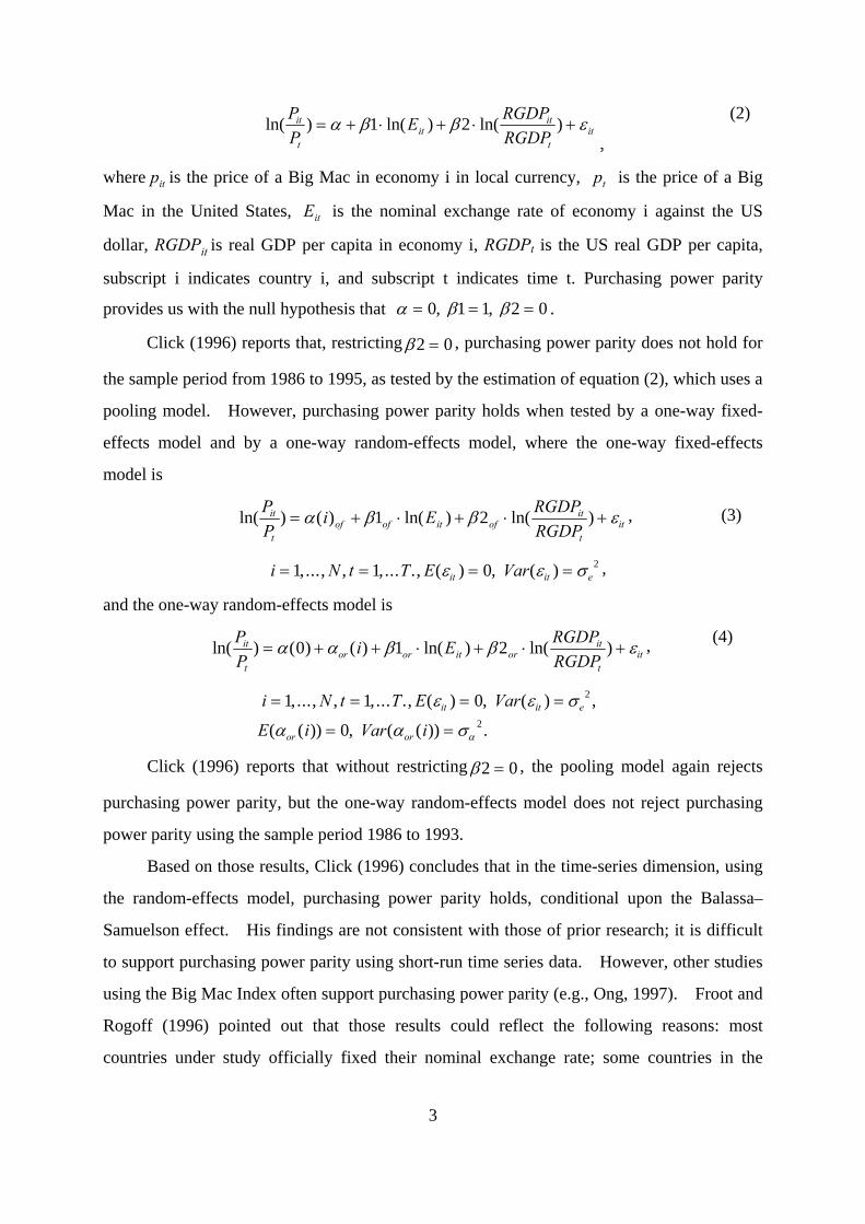
subscript i indicates country i, and subscript t indicates time t. Purchasing power parity

provides us with the null hypothesis that α β β= = =0 1 1 2 0, , .

Click (1996) reports that, restrictingβ2 0= , purchasing power parity does not hold for

the sample period from 1986 to 1995, as tested by the estimation of equation (2), which uses a

pooling model. However, purchasing power parity holds when tested by a one-way fixed-

effects model and by a one-way random-effects model, where the one-way fixed-effects

model is

ln( ) ( ) ln( ) ln( )PP

i E RGDPRGDP

it

tof of it of

it

tit= + ⋅ + ⋅ +α β β ε1 2 ,

, i N t T E Varit it e= = = =1 1 0 2,..., , , ... . ( ) , ( )ε ε σ ,

(3)

and the one-way random-effects model is

ln( ) ( ) ( ) ln( ) ln( )PP

i E RGDPRGDP

it

tor or it or

it

tit= + + ⋅ + ⋅ +α α β β ε0 1 2 ,

i N t T E Var

E i Var iit it e

or or

= = = =

= =

1 1 0

0

2

2

, ..., , , ... ., ( ) , ( ) ,

( ( )) , ( ( )) .

ε ε σ

α α σα

(4)

Click (1996) reports that without restrictingβ2 0= , the pooling model again rejects

purchasing power parity, but the one-way random-effects model does not reject purchasing

power parity using the sample period 1986 to 1993.

Based on those results, Click (1996) concludes that in the time-series dimension, using

the random-effects model, purchasing power parity holds, conditional upon the Balassa–

Samuelson effect. His findings are not consistent with those of prior research; it is difficult

to support purchasing power parity using short-run time series data. However, other studies

using the Big Mac Index often support purchasing power parity (e.g., Ong, 1997). Froot and

Rogoff (1996) pointed out that those results could reflect the following reasons: most

countries under study officially fixed their nominal exchange rate; some countries in the

4

sample experienced hyperinflation during the periods of estimation; and McDonald’s quickly

adjusts the price of the Big Mac.

In this paper, we use a statistical test to choose the most suitable empirical model for

testing purchasing power parity, and examine whether purchasing power parity holds,

following Fujiki and Kitamura (1995).

First, we compare the pooling model with the fixed-effects model, based on the F-test

(see Greene, 2000, for details). We also compare the fixed-effects model and the random-

effects model, using the Hausman test. Under the null hypothesis E i Xor it( ( ) )α = 0 , where

X is the explanatory variable in the regression, ( $ $ ) [ ( $ $ )] ( $ $ )'β β β β β βor of or of or ofVar− − −−1

follows a χ2 distribution whose degree of freedom is equal to Dim(βor

^). The decision rule is

that if the Hausman test statistic is significantly large, we should reject βor

^and accept βof

^.

We can also use the standard Lagrange Multiplier (LM) test to compare the pooling model

with the random-effects model. The decision rule is that the larger the LM test statistic, the

more likely is rejection of the pooling model and acceptance of the random-effects model.

Second, we incorporate the suggestion made by Froot and Rogoff (1996), and drop an

economy from our sample if that economy experiences changes in exchange rate regimes,

which usually results in hyperinflation.

Third, Froot and Rogoff (1996) conjectured that McDonald’s adjustment of price

depends on the nature of the shock, and in turn affects the results of the purchasing power

parity test. This point is quite compelling in the literature on pricing to the market.

Without large enough shocks, firms do not change their prices quickly. To test this idea,

suppose that the desired level of relative price considered by McDonald’s, )ln( **tit PP , can

be approximated as equation (5):

**

*

)ln(*2)ln(*1*)0()ln( itt

itit

t

it

RGDPRGDP

EPP

εββα +⋅+⋅+= . (5)

However, suppose that actual adjustment of price follows a linear mechanism, such that

price is adjusted to maintain some constant proportionate gap between desired and actual

price, as shown in the following equation:

5

it

t

it

t

it

t

it

t

it uPP

PP

PP

PP

+−⋅=−−

−

−

− )}ln(){ln(*)ln()ln(1

1*

*

1

1 γ . (6)

Then, we could compute the speed of adjustment by running equation (7):

it

t

it

t

itDPitDPDP

t

it

PP

RGDPRGDP

EPP

εγββα +⋅+⋅+⋅+=−

− )ln()ln(2)ln(1)0()ln(1

1 , (7)

where **)0()0( γαα =DP , **)1()1( γββ =DP , **)2()2( γββ =DP , **γε ititit uu += ,

*1 γγ −= . One can define the long-run elasticity of McDonald’s pricing with respect to

market exchange rate as β1DP/ (1- γ). Depending on the assumption whether DP)0(α is fixed

or random, a fixed-effects (FE) model or a random-effects (RE) model is used to estimate

equation (7).

A standard method applicable to a dynamic panel data model is the instrumental

variable (IV) or generalized method of moments estimator (GMM) of equation (7).1 However,

Monte Carlo studies conducted by Hsiao, Pesaran, and Tahmiscioglu (2002) show that those

standard estimators are subject to serious bias and size distortion in a finite sample, in

particular, if γ is close to one. To check robustness, we also provide a minimum distance

estimator (MDE) for the fixed-effects model, and generalized least squares (GLS)

supplemented with the initial value problem suggested by Hsiao (1986) for the random effects

model. Fujiki, Hsiao and Shen (2002) briefly review the merits of using MDE and GLS in

their statistical appendix.

3. Data

Following Click (1996), we use the data published in The Economist (1986–2002, various

issues) for the price of a Big Mac and the nominal exchange rate. We obtain data for

relative income from shares of aggregate GDP based on purchasing power parity, the basis for

the country weights used to generate the World Economic Outlook, April 2003, published by

the International Monetary Fund.2 The data are expressed as a percentage of the world total.

Thus, the ratio for the US share divided by the ratio of population to the US will replicate

purchasing power parity base relative income per capita. Population figures are also

1 See for example, Ahn and Schmidt (1995), and Arellano and Bover (1995). 2 All datasets are downloaded from http://www.imf.org/external/pubs/ft/weo/2003/01/data/index.htm.

6

available from the World Economic Outlook, April 2003.

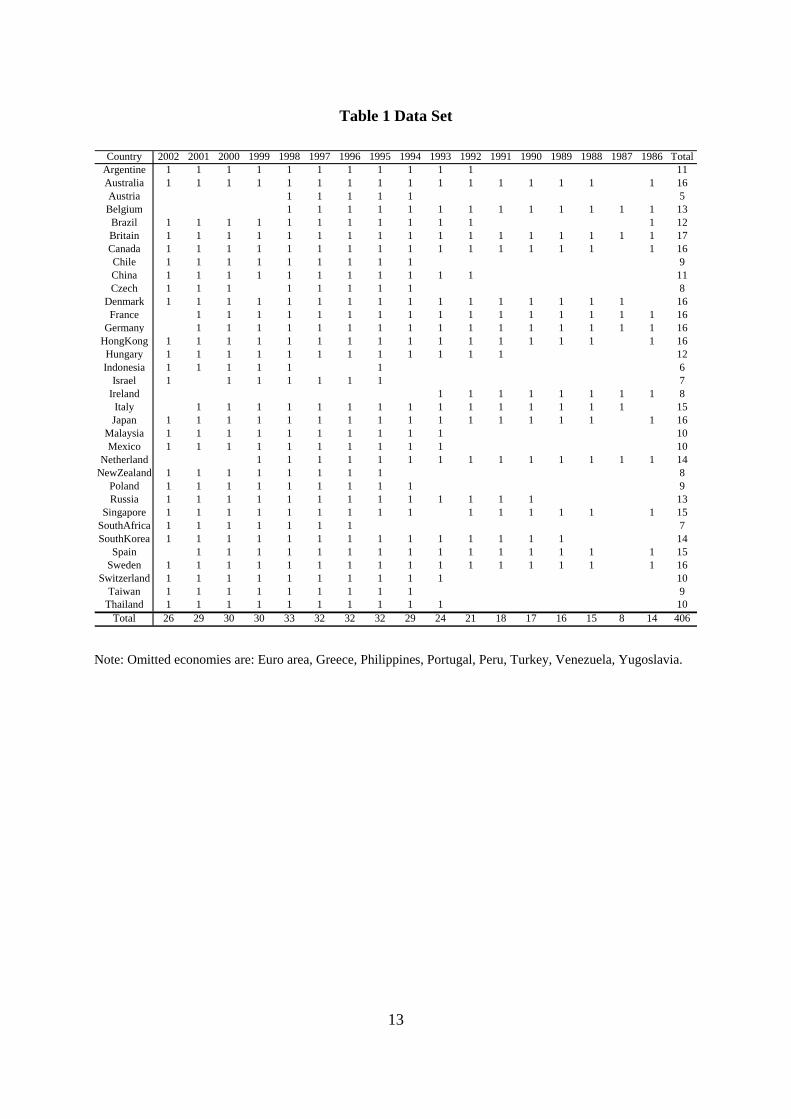
Unfortunately, the panel data set provided by The Economist is not an ideal balanced

panel data set. As Table 1 shows, we survey 34 economies between the year 1986 and 2002,

yielding 406 observations. However, only Britain was surveyed in all surveys. Some

economies are only rarely surveyed. For example, Greece, Portugal, and Venezuela were

surveyed only once, and thus are omitted from the analysis. We also omit the data on

Yugoslavia since we have no data on relative GDP. Moreover, since the 2002 survey, the

Euro-area economies, France, Germany and Spain, were not surveyed.

If one focuses the analysis between the year 1996 and 2002, we have a balanced panel

of 23 economies: Argentine, Australia, Brazil, Britain, Canada, Chile, China, Denmark, Hong

Kong, Hungary, Japan, Malaysia, Mexico, New Zealand, Poland, Russia, Singapore, South

Africa, South Korea, Sweden, Switzerland, Taiwan, and Thailand. Thus, it is interesting to

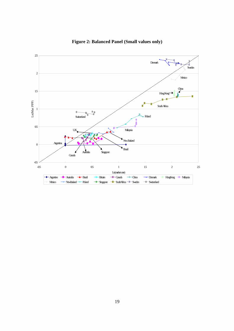
investigate the results using only that sub-sample of economies. Figure 1 plots all

observations from 1996 to 2002 for those 23 economies. It is tempting to conclude that

purchasing power parity holds, since most observations are on the 45-degree line. However,

as Figure 2 and Figure 3 show, an economy’s movement over time might not always lie above

the 45-degree line, and thus one might well consider that a fixed-effects estimator that

emphasizes time series variation within an economy could give us dramatically different

results. Moreover, the data on Russia look very unstable before and after the Russian

currency crisis in 1998. Argentina’s data shows an unusual jump in 2002, since it

abandoned its currency board. One might expect that in such a situation, a one-way fixed-

effects model will give us smaller estimates compared with a pooling model.

4. Results of Regressions

(1) Results using unbalanced panel data sets

The first three rows of Table 2 report our estimation of equations (2), (3) and (4) using

the sample period of 1986–2002 holdingβ2 0= . The pooling model, model (1), yields β

1=0.99312 and α=-0.0606. The F-value to test the joint null hypothesis of α β= =0 1 1, is

6.5669, and its p-value is 0.0016. Therefore, the pooling model rejects purchasing power

parity. However, the F-value for the one-way fixed-effects model, model (2), which tests the

one-way fixed-effects model versus the null hypothesis of the pooling model, is 34.117;

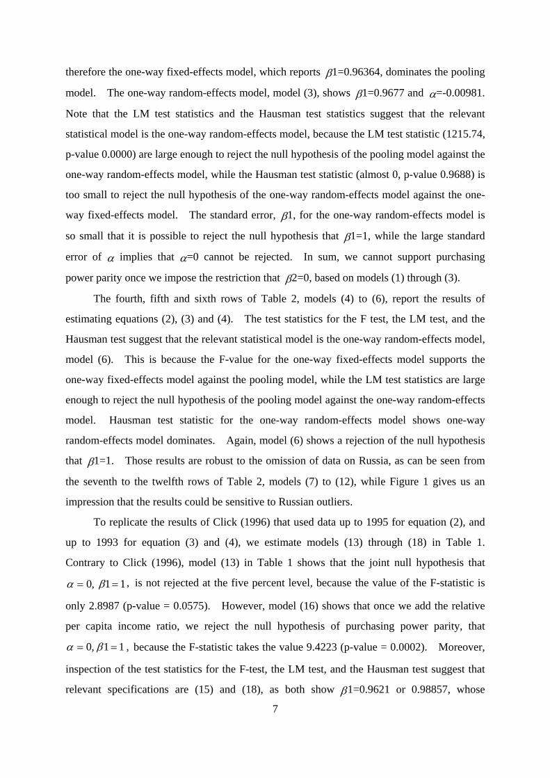
7

therefore the one-way fixed-effects model, which reports β1=0.96364, dominates the pooling

model. The one-way random-effects model, model (3), shows β1=0.9677 and α=-0.00981.

Note that the LM test statistics and the Hausman test statistics suggest that the relevant

statistical model is the one-way random-effects model, because the LM test statistic (1215.74,

p-value 0.0000) are large enough to reject the null hypothesis of the pooling model against the

one-way random-effects model, while the Hausman test statistic (almost 0, p-value 0.9688) is

too small to reject the null hypothesis of the one-way random-effects model against the one-

way fixed-effects model. The standard error, β1, for the one-way random-effects model is

so small that it is possible to reject the null hypothesis that β1=1, while the large standard

error of α implies that α=0 cannot be rejected. In sum, we cannot support purchasing

power parity once we impose the restriction that β2=0, based on models (1) through (3).

The fourth, fifth and sixth rows of Table 2, models (4) to (6), report the results of

estimating equations (2), (3) and (4). The test statistics for the F test, the LM test, and the

Hausman test suggest that the relevant statistical model is the one-way random-effects model,

model (6). This is because the F-value for the one-way fixed-effects model supports the

one-way fixed-effects model against the pooling model, while the LM test statistics are large

enough to reject the null hypothesis of the pooling model against the one-way random-effects

model. Hausman test statistic for the one-way random-effects model shows one-way

random-effects model dominates. Again, model (6) shows a rejection of the null hypothesis

that β1=1. Those results are robust to the omission of data on Russia, as can be seen from

the seventh to the twelfth rows of Table 2, models (7) to (12), while Figure 1 gives us an

impression that the results could be sensitive to Russian outliers.

To replicate the results of Click (1996) that used data up to 1995 for equation (2), and

up to 1993 for equation (3) and (4), we estimate models (13) through (18) in Table 1.

Contrary to Click (1996), model (13) in Table 1 shows that the joint null hypothesis that

α β= =0 1 1, , is not rejected at the five percent level, because the value of the F-statistic is

only 2.8987 (p-value = 0.0575). However, model (16) shows that once we add the relative

per capita income ratio, we reject the null hypothesis of purchasing power parity, that

11 ,0 == βα , because the F-statistic takes the value 9.4223 (p-value = 0.0002). Moreover,

inspection of the test statistics for the F-test, the LM test, and the Hausman test suggest that

relevant specifications are (15) and (18), as both show β1=0.9621 or 0.98857, whose

8

standard errors are 0.01 and 0.02, respectively. Therefore, over-all, the results shown in

Table 2 replicate the results of Click (1996) that purchasing power parity conditional upon the

Balassa–Samuelson effect works only in a limited case, (model (18)). Our different results

could be explained by different estimates of purchasing power parity base income per capita

made since the study of Click (1996).

(2) Results using balanced panel data sets

A. Basic Results

Our estimates of equations (2), (3) and (4) using balanced panel data are summarized in Table

3. Inspection of Table 3 shows that, based on the pooling model, models (19) and (22) seem

to support purchasing power parity. However, in both models, the null hypothesis of

purchasing power parity, that 11 ,0 == βα , is rejected because F-statistics take the value of

39.5854 and 45.6081. Indeed, the statistically preferred model in this table is the random-

effects model where the income ratio variable is omitted (model (21)), while including the log

of income ratio variable results in the statistically preferred model being the fixed-effects

model (24). It is interesting that the coefficients β1 are very close to one, irrespective of

specifications, and with or without income ratio variables.

B. Russian Outliers?

Following the suggestion of Froot and Rogoff (1996), that an economy hit by hyperinflation

could lead to evidence favorable to purchasing power parity, we drop observations for Russia

from the dataset. The results are summarized as models (25) to (30) in Table 3. Observe

that models (25) and (28) still show quite similar results to models (19) and (22). However,

regarding the fixed-effects model and random-effects model, the value of the coefficient of β1

falls substantially from one, and apparently rejects the null hypothesis of purchasing power

parity. Therefore, the results using this small balanced panel seem to be sensitive to the

inclusion of outliers, especially when one employs either the fixed-effects model or the

random-effects model.

C. Exchange Rate Regimes

The previous section shows that the results of using this small panel might be sensitive to the

9

inclusion of outliers. One could easily imagine that large jumps, or outliers, in the exchange

rate data should happen when speculative attacks occur. In this context, it is useful to see

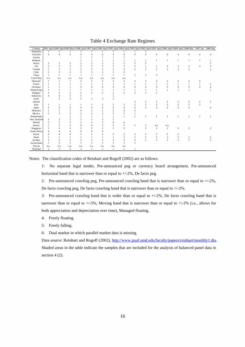
whether there are changes in exchange rate regimes during the sample period. Table 4

reports the classification codes of exchange rate regimes proposed by Reinhart and Rogoff

(2002). Shaded areas in the table indicate the samples which are included for the analysis of

the balanced panel data set. As we can see, we could exclude Brazil, Malaysia, and Korea,

as well as Thailand and Russia, since those economies experienced currency crises and thus

the codes are renumbered between the years 1996 and 2001. Reinhart’s and Rogoff’s (2002)

data cover up to 2001, and thus we also exclude Argentina. We end up with seven years of

data on 17 economies, in total, 119 observations.

Models (31) to (36) shown in Table 3 suggest that a reasonable model for this particular

sample is the one-way fixed-effects model with or without the relative GDP ratio, and the

estimates of coefficients on market exchange rate are far below one. Overall, evidence

shows that while the pooling model seems to be robust to the choice of sample economies, the

other two models are not.

D. McDonald’s Pricing Behavior?

It is true that, given the income ratio, models (23), (29) and (35) in Table 3 show that the

relative price of a Big Mac with respect to the US price level is relatively expensive in richer

economies than the market nominal exchange rate suggests. Hence, one may argue that the

Balassa–Samuelson effect might not be the sole reason for departure from purchasing power

parity. For example, one could interpret the results as a deliberate price setting behavior for

the Big Mac by McDonald’s, as Froot and Rogoff (1996) suggested.

To check this idea indirectly, one can estimate a dynamic panel data model and infer

the dynamic adjustment mechanism. Table 5 summarizes the results for equation (7). As

can be seen from the first to the sixth rows of Table 5 (models (37) to (40)), the estimated

parameter values of γ, responses from the lagged dependent variables, are small positive

values and take at most 0.3 irrespective of the choice of estimation methods, and the

coefficient on the current market exchange rate, β1, is still close to one, given the relative

GDP ratio. MDE might work better than the IV or GMM in a finite sample; however, since

γ is at most 0.3 in model (37), there is no reason to believe that model (38) is superior to

model (37). Moreover, long-run elasticity of McDonald’s pricing with respect to the market

10

exchange rate, β1/(1-γ), is also close to one, except for model (37). These results are

consistent with the idea that McDonald’s responds to fluctuations of nominal exchange rates

quickly, and almost one-to-one.

However, once we drop the data on Russia (models (41) to (44)), or use the samples of

stable exchange rate economies (models (45) to (48)), the estimates of β1 take values close to

zero, and are statistically insignificant except for GLS (models (44) and (48)). Moreover, γ

becomes close to one and in some case even exceeds one (models (41) and (42)). Therefore,

the application of dynamic panel data models to this particular small data set seems to be

risky, especially because it seems to be sensitive to the inclusion of outliers. Thus, it is

premature to conclude that dynamic panel data models provide strong evidence for rapid

adjustment of sale price by McDonald’s.

5. Summary and Conclusion

Evidence that purchasing power parity holds, conditional on the Balassa–Samuelson effect, as

reported in Click (1996), is not robust to the choice of methods of estimation, sample

economy and sample periods. In addition, one should be careful about the measurement

problems inherent in the Big Mac index, which we ignore in this paper. For example, as the

index is created from data collected only at one time in a year, that time might coincide with

transitory exchange rate fluctuations that do not reflect exchange rates throughout a year.

11

References

Ahn, S. C., Schmidt, P., 1995, Efficient estimation of models for dynamic panel data. Journal of Econometrics 68, 5-27.

Arellano, M., Bover, O., 1995, Another look at the instrumental variable estimation of error-components models. Journal of Econometrics 68, 29-51.

Balassa, B., 1963, The purchasing power parity doctrine: A reappraisal. Journal of Political

Economy 72, 231-238. Baltagi, H. B., 2001, Econometric Analysis of Panel Data, 2nd ed. John Wiley and Sons, New

York.

Click, R. W., 1996, Contrarian MacParty. Economics Letters 53, 209-212. Dickey, D. A., and W. A. Fuller, 1979, Distributions of the Estimators for Autoregressive

Time Series with a Unit Root. Journal of the American Statistical Association 75, 427-431.

Dickey, D. A., and W. A. Fuller, 1981, Likelihood Ratio Statistics for Autoregressive Time

Series with a Unit Root. Econometrica 49, 1057-1072 Engel, R. F., and C. W. J. Granger, 1987, Cointegration and Error Correction: Representation,

Estimation and Testing. Econometrica 55, 251-276. Fujiki, H. and Y. Kitamura, 1995, Feldstein-Horioka Paradox Revisited. Bank of Japan,

Monetary and Economic Studies 13, 1, 1-16.

―――, C. Hsiao, and Y. Shen, 2002, Is There a Stable Money Demand Function under the Low Interest Rate Policy? A Panel Data Analysis, Bank of Japan, Monetary and Economic Studies 20, 2, 1-23.

Froot, K. A. and K. Rogoff, 1996, Perspectives on PPP and Long-Run Real Exchange Rate.

In: Gene Grossman and Kenneth Rogoff (eds), Handbook of International Economics, Vol. 3, North Holland, Amsterdam.

Green, W. H., 2000, Econometric Analysis, 4th ed., Prentice Hall, New York.

12

Hsiao, C., 1986, Analysis of Panel Data, Cambridge University Press, Cambridge. ———, M. H. Pesaran, and A. K. Tahmiscioglu, 2002, Maximum Likelihood Estimation of

Fixed Effects Dynamic Panel Data Models Covering Short Time Periods. Journal of Econometrics 109, 107-150.

Nelson, C Mark, 2001, International Macroeconomics and Finance: Theory and Econometric Methods, Blackwell Publishers.

Ong, L., 1997, Burgernomics: The Economics of the Big Mac Standard. Journal of

International Money and Finance 16, 865-878. Pakko, M. R. and P. S. Pollard, January/February 1996, For Here or To GO? Purchasing

Power Parity and the Big Mac. Federal Reserve Bank of St. Louis Review.

Reinhart C. M., and K. Rogoff, 2002, The Modern History of Exchange Rate Arrangements: A Reinterpretation, NBER Working Paper No. 8963.

Rogoff, K., 1996, The Purchasing Power Parity Puzzle. Journal of Economic Literature, 34,

647-668. Phillips, P. C. B., 1986, Understanding Spurious Regressions in Econometrics. Journal of

Econometrics 33, 311-340. Phillips, P. C. B., and S. N. Durlauf, 1986, Multiple Time Series Regression with Integrated

Processes. Review of Economics Studies 53, 473-495. Samuelson, P. A., 1964, Theoretical Notes on Trade Problems, Review of Economics and

Statistics 46, 145-154. Wu, Y., 1996,Are Real Exchange Rates Nonstationary? Evidence from a Panel Data Test.

Journal of Money, Credit and Banking, 28, 54-63.

13

Table 1 Data Set

Country 2002 2001 2000 1999 1998 1997 1996 1995 1994 1993 1992 1991 1990 1989 1988 1987 1986 TotalArgentine 1 1 1 1 1 1 1 1 1 1 1 11Australia 1 1 1 1 1 1 1 1 1 1 1 1 1 1 1 1 16Austria 1 1 1 1 1 5Belgium 1 1 1 1 1 1 1 1 1 1 1 1 1 13Brazil 1 1 1 1 1 1 1 1 1 1 1 1 12Britain 1 1 1 1 1 1 1 1 1 1 1 1 1 1 1 1 1 17Canada 1 1 1 1 1 1 1 1 1 1 1 1 1 1 1 1 16Chile 1 1 1 1 1 1 1 1 1 9China 1 1 1 1 1 1 1 1 1 1 1 11Czech 1 1 1 1 1 1 1 1 8

Denmark 1 1 1 1 1 1 1 1 1 1 1 1 1 1 1 1 16France 1 1 1 1 1 1 1 1 1 1 1 1 1 1 1 1 16

Germany 1 1 1 1 1 1 1 1 1 1 1 1 1 1 1 1 16HongKong 1 1 1 1 1 1 1 1 1 1 1 1 1 1 1 1 16Hungary 1 1 1 1 1 1 1 1 1 1 1 1 12Indonesia 1 1 1 1 1 1 6

Israel 1 1 1 1 1 1 1 7Ireland 1 1 1 1 1 1 1 1 8Italy 1 1 1 1 1 1 1 1 1 1 1 1 1 1 1 15Japan 1 1 1 1 1 1 1 1 1 1 1 1 1 1 1 1 16

Malaysia 1 1 1 1 1 1 1 1 1 1 10Mexico 1 1 1 1 1 1 1 1 1 1 10

Netherland 1 1 1 1 1 1 1 1 1 1 1 1 1 1 14NewZealand 1 1 1 1 1 1 1 1 8

Poland 1 1 1 1 1 1 1 1 1 9Russia 1 1 1 1 1 1 1 1 1 1 1 1 1 13

Singapore 1 1 1 1 1 1 1 1 1 1 1 1 1 1 1 15SouthAfrica 1 1 1 1 1 1 1 7SouthKorea 1 1 1 1 1 1 1 1 1 1 1 1 1 1 14

Spain 1 1 1 1 1 1 1 1 1 1 1 1 1 1 1 15Sweden 1 1 1 1 1 1 1 1 1 1 1 1 1 1 1 1 16

Switzerland 1 1 1 1 1 1 1 1 1 1 10Taiwan 1 1 1 1 1 1 1 1 1 9

Thailand 1 1 1 1 1 1 1 1 1 1 10Total 26 29 30 30 33 32 32 32 29 24 21 18 17 16 15 8 14 406

Note: Omitted economies are: Euro area, Greece, Philippines, Portugal, Peru, Turkey, Venezuela, Yugoslavia.

14

Table 2 Results of Regressions

Dependent Variable = Ln(P(i,t)/P(t))Sample Model Methods R2 F LM Hausman

(p-value) (p-value) (p-value)1986-2002 (1) Pool -0.05060 0.99312 0.9744 6.5669(N=405) (S.E.) (0.0282) (0.0080) (0.0016)

(2) Fixed 0.96364 0.99312 34.117(S.E.) (0.1047) (0.0000)

(3) Random -0.00981 0.9677 0.9735 1215.74 0.00(S.E.) (0.0642) (0.0103) (0.0000) (0.9688)

1986-2002 (4) Pool -1.63913 1.01746 0.38821 0.9820 90.8853(N=405) (S.E.) (0.1246) (0.0070) (0.0299) (0.0000)

(5) Fixed 0.96994 0.39374 0.99324 21.341(S.E.) (0.1019) (3.5213) (0.0000)

(6) Random -1.4711 0.9818 0.3704 0.9735 1,043.15 0.01(S.E.) (0.2765) (0.0100) (0.0690) (0.0000) (0.9933)

1986-2002 (7) Pool -0.05625 0.99946 0.97443 4.4837(N=393) (S.E.) (0.0279) (0.0082) (0.0141)

Drop (8) Fixed 0.95937 0.99406 41.27400Russia (S.E.) (0.1455) (0.0000)

(9) Random 0.00293 0.96538 0.97263 1,267.68 0.00(S.E.) (0.0652) (0.0110) (0.0000) (0.9668)

1986-2002 (10) Pool -1.60412 1.02102 0.37862 0.98204 86.7188(N=393) (S.E.) (0.1233) (0.0070) (0.0296) (0.0000)

Drop (11) Fixed 0.96178 0.32747 0.99412 26.20200Russia (S.E.) (0.1462) (4.1161) (0.0000)

(12) Random -1.35875 0.97687 0.34497 0.97322 1,161.13 0.01(S.E.) (0.2809) (0.0105) (0.0702) (0.0000) (0.9945)

1986-1995 (13) Pool 0.05851 1.00358 0.97664 2.8987(N=193) (S.E.) (0.0388) (0.0111) (0.0575)

(14) Fixed 0.95378 0.99426 19.66000(S.E.) (0.1597) (0.0000)

(15) Random 0.11539 0.96217 0.97263 299.43 0.00(S.E.) (0.0704) (0.0132) (0.0000) (0.9589)

1986-1993 (16) Pool -1.31523 1.03332 0.32181 0.97931 9.4223(N=132) (S.E.) (0.3155) (0.0133) (0.0739) (0.0002)

(17) Fixed 0.94885 0.53617 0.99266 10.82400(S.E.) (0.5083) (10.3464) (0.0000)

(18) Random -1.21152 0.98857 0.32476 0.97322 126.50 0.01(S.E.) (0.4288) (0.0204) (0.1040) (0.0000) (0.9945)

α β1 β2

Notes: F value for the pooling model is the test statistic for the joint null hypothesis that α β= =0 1 1, .

F-value for the fixed-effects model compares the fixed-effects model versus the null hypothesis of the

pooling model. High values of LM favor the fixed-effects model and the random-effects model over

the pooling model. High (low) values of the Hausman test statistic favor the fixed-effects model

(random-effects model).

All estimations include data on Russia except in the year 1990, where the income ratio data are missing.

Thus, total observations are 405 in the case for equations (1) thought (3), rather than 406 shown in table

1.

15

Table 3 Results of Regressions

Dependent Variable = Ln(P(i,t)/P(t))Sample Model Methods R2 F LM Hausman

(p-value) (p-value) (p-value)1996-2002 (19) Pool -0.23985 0.99665 0.97357 39.5854(N=161) (S.E.) (0.0414) (0.0130) (0.0020)

(20) Fixed 0.99289 0.99328 22.19900(S.E.) (0.0368) (0.0000)

(21) Random -0.23457 0.99441 0.97881 267.6 0.00000(S.E.) (0.0795) (0.0193) (0.0000) (0.9611)

1996-2002 (22) Pool -1.49649 1.01119 0.32408 0.98110 45.6081(N=161) (S.E.) (0.1605) (0.0111) (0.0404) (0.0000)

(23) Fixed 1.02447 1.66771 0.99461 19.01(S.E.) (0.0300) (0.4936) (0.0000)

(24) Random -1.94981 1.00813 0.44619 0.97952 213.9 7.46000(S.E.) (0.3459) (0.0170) (0.0883) (0.0000) (0.0240)

1996-2002 (25) Pool -0.23406 0.99818 0.96944 34.50(N=154) (S.E.) (0.0427) (0.0143) (0.0020)

Drop (26) Fixed 0.22817 0.99832 125.23Russia (S.E.) (0.0595) (0.0000)

(27) Random 0.62869 0.60812 0.97881 263.5 50.34(S.E.) (0.0937) (0.0260) (0.0000) (0.0000)

1996-2002 (28) Pool -1.47069 1.00731 0.32006 0.97787 41.2105(N=154) (S.E.) (0.1651) (0.0122) (0.0417) (0.0000)

Drop (29) Fixed 0.30291 0.83705 0.99866 112.00Russia (S.E.) (0.0419) (0.1918) (0.0000)

(30) Random -2.02631 0.66663 0.66451 0.97952 215.3 142.51(S.E.) (0.3456) (0.0232) (0.0856) (0.0000) (0.0007)

1996-2002 (31) Pool -0.19998 0.99089 0.96203 23.18(N=119) (S.E.) (0.0504) (0.0181) (0.0000)

(32) Fixed 0.36074 0.99810 139.69(S.E.) (0.0605) (0.0000)

(33) Random 0.42750 0.69668 0.97881 270.2 45.27(S.E.) (0.1110) (0.0342) (0.0000) (0.0000)

1996-2002 (34) Pool -1.62186 1.01619 0.34724 0.97377 35.5355(N=119) (S.E.) (0.1991) (0.0155) (0.0475) (0.0000)

(35) Fixed 0.35069 0.74390 0.99833 107.38(S.E.) (0.0502) (0.2435) (0.0000)

(36) Random -0.84763 0.74763 0.29610 0.97952 231.73 130.5(S.E.) (0.4225) (0.0302) (0.1025) (0.0000) (0.0007)

α β1 β2

Notes: Sample economies included after 1996 are: Argentina, Australia, Brazil, Britain, Canada, Chile, China,

Denmark, Hong Kong, Hungary, Japan, Malaysia, Mexico, New Zealand, Poland, Russia, Singapore,

South Africa, South Korea, Sweden, Switzerland, Taiwan, and Thailand. F-value for the pooling model is the test statistic for the joint null hypothesis that α β= =0 1 1, .

F-value for the fixed-effects model compares the fixed-effects model versus the null hypothesis of the

pooling model. High values of LM favor the fixed-effects model and the random-effects model over

the pooling model. High (low) values of the Hausman test statistic favor the fixed-effects model

(random- effects model).

16

Table 4 Exchange Rate Regimes Country 2001 April 2000 April1999 March1998 April 1997 April 1996 April 1995 April 1994 April 1993 April 1992 April 1991 April 1990 April 1989 April 1988 Mar. 1987 Jan. 1986 Sep.

Argentina 1 1 1 1 1 1 1 1 1 1Australia 4 4 4 4 4 4 4 4 4 4 4 4 4 4 4 4Austria 1 1 1 1 1Belgium 1 1 1 1 1 1 1 1 1 1 1 1 1Brazil 3 3 5 2 2 2 2 5 5 5 5UK 3 3 3 3 3 3 3 3 3 1 1 3 3 3 3 3

Canada 2 2 2 2 2 2 2 2 2 2 2 2 2 2 2Chile 3 3 3 3 3 3 3 3China 1 1 1 1 1 1 1 1 2 3 3

Czech Rep n.a. n.a. n.a. n.a. n.a. n.a. n.a. n.a.Denmark 1 1 1 2 2 2 2 2 2 2 2 2 2 2 2France 1 1 1 1 1 1 1 1 1 1 1 1 1 1 1 2

Germany 1 1 1 4 4 4 4 4 4 4 4 4 4 4 4 4Hong Kong 1 1 1 1 1 1 1 1 1 1 1 1 1 1 1

Hungary 3 3 3 2 2 2 2 3 3 3 3Indonesia 4 4 5 5 2

Israel 3 3 3 3 3 3Ireland 2 2 2 2 2 2 2 2

Italy 1 1 1 1 1 2 2 2 2 2 2 2 2 2 2Japan 4 4 4 4 4 4 4 4 4 4 4 4 4 4 4

Malaysia 1 1 1 4 2 2 2 2 2Mexico 3 3 3 3 3 3 5 3 1

Netherlands 1 1 1 1 1 1 1 1 1 1 1 1 1 1New Zealand 3 3 3 3 3 3 3

Poland 3 3 3 3 3 3 6 6Russia 2 2 5 6 6 5 5 5 5 5 n.a. n.a.

Singapore 3 3 3 2 2 2 2 2 2 2 2 2 2 2South Africa 4 4 4 4 4 4

Korea 4 4 4 5 2 2 2 2 2 2 2 2 2Spain 1 1 1 1 1 1 1 2 2 2 2 2 2 2 2

Sweden 3 3 3 3 3 3 3 3 3 2 2 2 2 2 2Switzerland 2 2 2 2 2 2 2 2 2

Taiwan n.a. n.a. n.a. n.a. n.a. n.a. n.a. n.a.Thailand 3 3 3 3 1 1 1 1 1

Notes: The classification codes of Reinhart and Rogoff (2002) are as follows:

1: No separate legal tender, Pre-announced peg or currency board arrangement, Pre-announced

horizontal band that is narrower than or equal to +/-2%, De facto peg.

2: Pre-announced crawling peg, Pre-announced crawling band that is narrower than or equal to +/-2%,

De facto crawling peg, De facto crawling band that is narrower than or equal to +/-2%.

3: Pre-announced crawling band that is wider than or equal to +/-2%, De facto crawling band that is

narrower than or equal to +/-5%, Moving band that is narrower than or equal to +/-2% (i.e., allows for

both appreciation and depreciation over time), Managed floating.

4: Freely floating.

5: Freely falling.

6: Dual market in which parallel market data is missing.

Data source: Reinhart and Rogoff (2002), http://www.puaf.umd.edu/faculty/papers/reinhart/monthly1.dta.

Shaded areas in the table indicate the samples that are included for the analysis of balanced panel data in

section 4 (2).

17

Table 5 Results of Regressions

Dependent Variable = Ln(P(i,t)/P(t)), Sample 1996-2002Methods and samples Model Methods α β 1 β 2 γ Long Run

ElasticityIV (37) Fixed 1.0296 2.9079 0.2950 1.4604

(N=161) (S.E.) (0.0371) (0.5046) (0.0355) MDE (38) Fixed 0.9550 1.7026 0.1114 1.0747

(N=161) (S.E.) (0.0278) (0.2487) (0.0250) IV (39) Random -1.47075 0.9752 0.3106 0.0389 1.0147

(N=161) (S.E.) (0.6245) (0.1892) (0.1537) (0.1834) GLS (40) Random -5.4058 0.9515 1.3084 0.1476 1.1163

(N=161) (S.E.) (21.8564) (0.0426) (0.3588) (0.0325) IV (41) Fixed 0.0341 -0.1741 1.0472 -0.7232

(N=154, drop Russia) (S.E.) (0.0805) (0.3503) (0.1418) MDE (42) Fixed 0.1136 0.1764 1.0788 -1.4410

(N=154, drop Russia) (S.E.) (0.0351) (0.0918) (0.0452) IV (43) Random -0.22948 0.2055 0.0467 0.8018 1.0366

(N=154, drop Russia) (S.E.) (1.3292) (0.7633) (0.2944) (0.7581) GLS (44) Random -0.9633 0.1847 0.3976 0.5200 0.3848

(N=154, drop Russia) (S.E.) (1.3907) (0.0702) (0.2805) (0.1411) IV (45) Fixed 0.0056 0.1234 0.8996 0.0557

(N=119) (S.E.) (0.1220) (0.4537) (0.1542) MDE (46) Fixed 0.0659 0.3004 0.9842 4.1735

(N=119) (S.E.) (0.0554) (0.1337) (0.0616) IV (47) Random -0.2969 0.2481 0.0605 0.7602 1.0347

(N=119) (S.E.) (1.8982) (1.0276) (0.4085) (1.0121) GLS (48) Random -1.4810 0.5368 0.175145 0.5089 1.0930

(N=119) (S.E.) (1.4587) (0.1510) 0.096664 (0.3368)

18

Figure 1：Whole sample

-1

0

1

2

3

4

5

6

7

8

9

-1 0 1 2 3 4 5 6 7 8 9

Ln(market rate)

Ln(M

ac P

PP)

Argentine Australia Brazil Britain Canada Chile China Denmark HongKong Hungary Japan MalaysiaMexico NewZealand Russia Singapore SouthAfrica SouthKorea Sweden Switzerland Taiwan Thailand

Russia

19

Figure 2: Balanced Panel (Small values only)

-0.5

0

0.5

1

1.5

2

2.5

-0.5 0 0.5 1 1.5 2 2.5

Ln(market rate)

Ln(M

ac P

PP)

Argentine Australia Brazil Britain Canada China Denmark HongKong MalaysiaMexico NewZealand Poland Singapore SouthAfrica Sweden Switzerland

DenmarkSweden

Mexico

ChinaHong Kong

South Africa

Malaysia

PolandSwitzerland

Argentina

CanadaAustralia Singapore

Brazil

New Zealand

U.K.

20

Figure 3: Balanced Panel (Large values only)

2.5

3

3.5

4

4.5

5

5.5

6

6.5

7

7.5

8

8.5

9

2.5 3 3.5 4 4.5 5 5.5 6 6.5 7 7.5 8 8.5 9

ln(market rate)

ln(M

ac p

pp)

Chile Hungary Japan SouthKorea Taiwan Thailand Russia

Thailand

Taiwan

HungaryJapan

Chile

Korea

Russia

1996-98

1999-2002, Russia