Discovering Geometric Patterns in Genomic Data

Wenxuan Gao

Department of Computer

Science

University of Illinois at Chicago

wgao5@uic.edu

Christopher Brown

Institute for Genomics &

Systems Biology

caseybrown@uchicago.edu

Robert L. Grossman

Institute for Genomics &

Systems Biology

robert.grossman

@uchicago.edu

Lijia Ma

Institute for Genomics &

Systems Biology

ljma

@uchicago.edu

Matthew Slattery

Institute for Genomics &

Systems Biology

mgslattery

@uchicago.edu

Kevin P. White

Institute for Genomics &

Systems Biology

kpwhite@uchicago.edu

Philip S. Yu

Dept. of Computer Science

University of Illinois at Chicago

psyu@cs.uic.edu

ABSTRACTChIP-chip and ChIP-seq are techniques for the isolation andidentification of the binding sites of DNA-associated proteinsalong the genome. Both techniques produce genome-widelocation data. The geometric arrangements of these bind-ing sites can provide valuable information about biologicalfunction, such as the activation or repression of genes.

In this paper, we formalize this problem and propose anovel graph based algorithm called Patterns of Marks (PoM)to discover e�ciently these types of geometric patterns in ge-nomic data. We also describe how we validate the algorithmusing experimental data.

Categories and Subject DescriptorsJ.3 [Life and Medical Science]: Biology and genetics;H.2.8 [Database Management]: Database Applications—Data mining

General TermsAlgorithms

Keywordsgeometric pattern, DNA binding sites, graph mining

1. INTRODUCTIONThe genome has been sequenced for some time and a fun-

damental biological challenge now is to understand how ge-

Permission to make digital or hard copies of all or part of this work forpersonal or classroom use is granted without fee provided that copies arenot made or distributed for profit or commercial advantage and that copiesbear this notice and the full citation on the first page. To copy otherwise, torepublish, to post on servers or to redistribute to lists, requires prior specificpermission and/or a fee.ACM-BCB ’12, October 7-10, 2012, Orlando, FL, USACopyright 2012 ACM 978-1-4503-1670-5/12/10 ...$15.00.

nomic sequences code biological function. Biological func-tion is determined not just by genes, but also by genomicsequences that code repressors, activators, and other regu-latory structures, such as chromatin regulators, that deter-mine how genes are transcribed into RNA. There are labo-ratory techniques, such as ChIP-chip and ChIP-seq technol-ogy, that can help identify these types of regulatory struc-tures by attaching certain proteins to the genome at whatare called binding sites. The geometric combination of thesebinding sites provide valuable information about biologicalfunction and finding out such genomic patterns (A precisedefinition is given in Section 3.2) can o↵er new insight intothe mechanism of regulation.

In this paper, 1) we abstract and formalize this problemas the discovery of specific types of geometric patterns in ge-nomic data (Geometric Pattern Discovery); 2) we propose analgorithm called PoM for e�ciently discovering these typesof geometric patterns in genomic data based upon frequentsubgraphs; 3) we evaluate the PoM on experimental data tovalidate its usefulness.Marks along the genome. There are several di↵erenttypes of proteins that bind to certain regions along the genome.In this paper, we use the term chromatin factor to referto transcription factors and chromatin regulators, both ofwhich bind along the genome at binding sites. You canthink of these binding sites occurring in Regions of Inter-est (ROI) along the genome. For simplicity, in this paper,we abstract this simply as a mark along the genome associ-ated with a factor. A mark is not a single point along thegenome but rather an interval or region along the genome. Itis important to note there are many types of marks, depend-ing upon the specific protein that binds to the genome, andin general, each protein binds in multiple places along thegenome. This is contrary to many of the genomic patternsstudied previously in the KDD community involving gene-gene interactions, or gene-protein interactions, in which agene occurs in one region along the genome.Biological significance. Genome-wide protein-DNA bind-ing site data are now available for transcription factors and

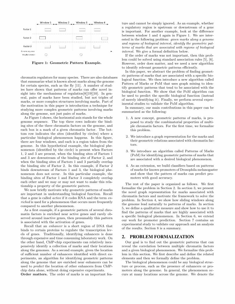
Figure 1: Geometric Pattern Example.

chromatin regulators for many species. There are also databasesthat summarize what is known about marks along the genomefor certain species, such as the fly [11]. A number of stud-ies have shown that patterns of marks can o↵er novel in-sight into the mechanisms of regulation[8][19][10]. In gen-eral, pairs of marks have been studied, but not triples ofmarks, or more complex structures involving marks. Part ofthe motivation in this paper is introduction a technique forstudying more complex geometric patterns involving marksalong the genome, not just pairs of marks.

As Figure 1 shows, the horizontal axis stands for the wholegenome sequence. The top three rows indicate the bind-ing sites of the three chromatin factors on the genome, andeach box is a mark of a given chromatin factor. The bot-tom row indicates the sites (identified by circles) where aparticular biological phenomenon happens. In this figure,there are four windows, and each is a region taken from thegenome. In this hypothetical example, the biological phe-nomenon (identified by the circle) is present when Factors1, 2 and 3 are present, when the binding sites of Factors 1and 3 are downstream of the binding site of Factor 2, andwhen the binding sites of Factors 1 and 3 partially overlapthe binding site of Factor 2. In this example, if Factor 2binds downstream of Factors 1 and 3, the biological phe-nomenon does not occur. In this particular example, thebinding sites of Factor 1 and Factor 3 completely overlapeach other and we may or may not want to make this rela-tionship a property of the geometric pattern.

We now briefly motivate why geometric patterns of marksare important in understanding biological function. Recallthat a gene is called active if it codes RNA and the term en-riched is used for a phenomenon that occurs more frequentlycompared to another phenomenon.

As a first example, if a geometric pattern of several chro-matin factors is enriched near active genes and rarely ob-served around inactive genes, then presumably this patternis associated with the activation of genes.

Recall that an enhancer is a short region of DNA thatbinds to certain proteins to regulate the transcription lev-els of genes. Traditionally, identifying enhancers is donethrough expensive and time consuming laboratory work. Onthe other hand, ChIP-chip experiments can relatively inex-pensively identify a collection of marks and their locationsalong the genomes. As a second example, given the locationof su�cient number of enhancers identified with direct ex-periments, an algorithm for identifying geometric patternsalong the genome that are enriched near enhancers can beused to predict the location of other enhancers from ChIP-chip data alone, without doing expensive experiments.Order matters. The order of marks is an important fea-

ture and cannot be simply ignored. As an example, whethera regulatory region is upstream or downstream of a geneis important. For another example, look at the di↵erencebetween window 1 and 4 again in Figure 1. We are inter-ested in the following problem: given marks along a genomeand regions of biological interest, identify the geometric pat-terns of marks that are associated with regions of biologicalinterest. We give a formal definition below.

If the order of marks was not important, then this prob-lem could be solved using standard association rules [5], [6].However, order does matter, and we need a new algorithmto identify relevant geometric patterns e�ciently.

In this paper, we abstract the problem of finding geomet-ric patterns of marks that are associated with a specific bio-logical function. We then introduce a new algorithm calledPattern of Marks or PoM that uses graph mining to iden-tify geometric patterns that tend to be associated with thebiological function. We show that the PoM algorithm canbe used to predict the specific biological function (insteadof merely identifying it). Finally, we perform several exper-imental studies to validate the PoM algorithm.

In summary, our main contributions in this paper can besummarized as the following:

1. A new concept, geometric patterns of marks, is pro-posed to study the combinatorial properties of multi-ple chromatin factors. For the first time, we formalizethis problem.

2. We introduce a graph representation for the marks andtheir geometric relations associated with chromatin fac-tors.

3. We introduce an algorithm called Patterns of Marks(PoM) for identifying geometric patterns of marks thatare associated with a desired biological phenomenon.

4. As an extension, we build classifiers based on patternsof marks for known promoters of Drosophila melanogasterand show that the pattern of marks can predict pro-moters with good accuracy.

The rest of the paper is organized as follows. We firstformalize the problem in Section 2. In section 3, we presentthe novel graph representation for marks associated withchromatin factors and motivate the framework to solve theproblem. In Section 4, we show how sliding windows alongthe genome lead naturally to patterns of marks. In section5, we define a qualitative measure and show how to use it tofind the patterns of marks that are highly associated witha specific biological phenomenon. In Section 6, we extendour work for promoter prediction. Section 7 contains anexperimental study to validate our approach and an analysisof the results. Section 8 is a summary.

2. PROBLEM FORMALIZATIONOur goal is to find out the geometric patterns that can

reveal the correlation between multiple chromatin factorsand a given biological phenomenon. We formalize this prob-lem in this section. We first describe and define the relatedelements and then we formally define the problem.

The biological phenomenon could be any biological struc-ture or process, such as the presence of enhancers or pro-moters along the genome. In general, the phenomenon oc-curs at many locations across the genome. We denote the

set of sites where that biological phenomenon happens asS = {s1, s2, s3, ...}, where each si is one such site. The sitesi is usually given as a point. However, sometimes it is givenas a region, with the start point vi and the end point wi ofthe region specified. In that case, we take si as the midpointsi = (vi + wi)/2.

We denote the (chromatin) factors as M1, M2, M3,..., andMn. Usually the binding sites of chromatin factors are givenas regions, which have start positions and stop positions.We call the regions marks or Regions of Interest(ROIs). Foreach chromatin factor Mi, the set of ROIs is denoted asRi= {R1

i ,R2i ,... Rki

i }, where ki is the number of ROIs forMi. Each ROI Rj

i has a start position denoted by Start(Rji )

and a stop position denoted by Stop(Rji ) on the genome.

In this paper, from the binding sites data of several chro-matin factors, we want to identify the geometric patternsthat are enriched1 around the sites of the given biologicalphenomenon while being rarely observed at a random po-sition across the whole genome. We denote such a set ofpatterns by P = {p1, p2, ...}, where each pi is a particulargeometric combination of ROIs of the involved chromatinfactors. In summary, the problem can be formalized as thefollowing:

Definition 1. Geometric Pattern Discovery. Assumethere are n factors M1, M2, M3,..., and Mn and that eachfactor has a set of binding sites along the genome that we callmarks or Regions of Interest (ROIs). Denote the ROIs of fac-tor Mi by {R1

i ,R2i ,... R

kii }, where ki is the number of ROIs

for Mi. Each Rji has a start position denoted by Start(Rj

i )and a stop position denoted by Stop(Rj

i ). Also assume thatacross the genome a specific biological phenomenon happensat a set of sites S = {s1, s2, s3, ...}. The goal is to identifygeometric patterns P = {p1, p2, ...} that occur nearby S witha much higher probability2 than that of a random positionon the genome, where pi is a geometric combination of ROIsof the involved factors.

Figure 1 contains an example. In this paper, we alwaysassume that patterns of marks are local in the sense thatare contained in a window. A simple example of a patternis to require that Factor 2 must occur before (upstream) ofFactor 1. This pattern occurs twice in this figure.

3. GRAPH THEORETIC FRAMEWORKIn this section, we introduce a graph theoretic framework

for representing geometric patterns of marks in genomicdata.

3.1 Basic Graph ConceptsIn this subsection, we introduce some basic graph concepts

related to our work.

Definition 2. Graph. A graph is denoted by g = (V,E),where V is a set of nodes and E is a set of edges connectingthe nodes. Both nodes and edges may have labels. In agraph, each node has a unique ID.1Biologists commonly use the term enriched to apply to aphenomenon that is more highly present than would be ex-pected from random behavior.2We are also interested in geometric patterns that occurwith a much lower probability than would be expected ifthere were no relationship between the marks and the sitesS.

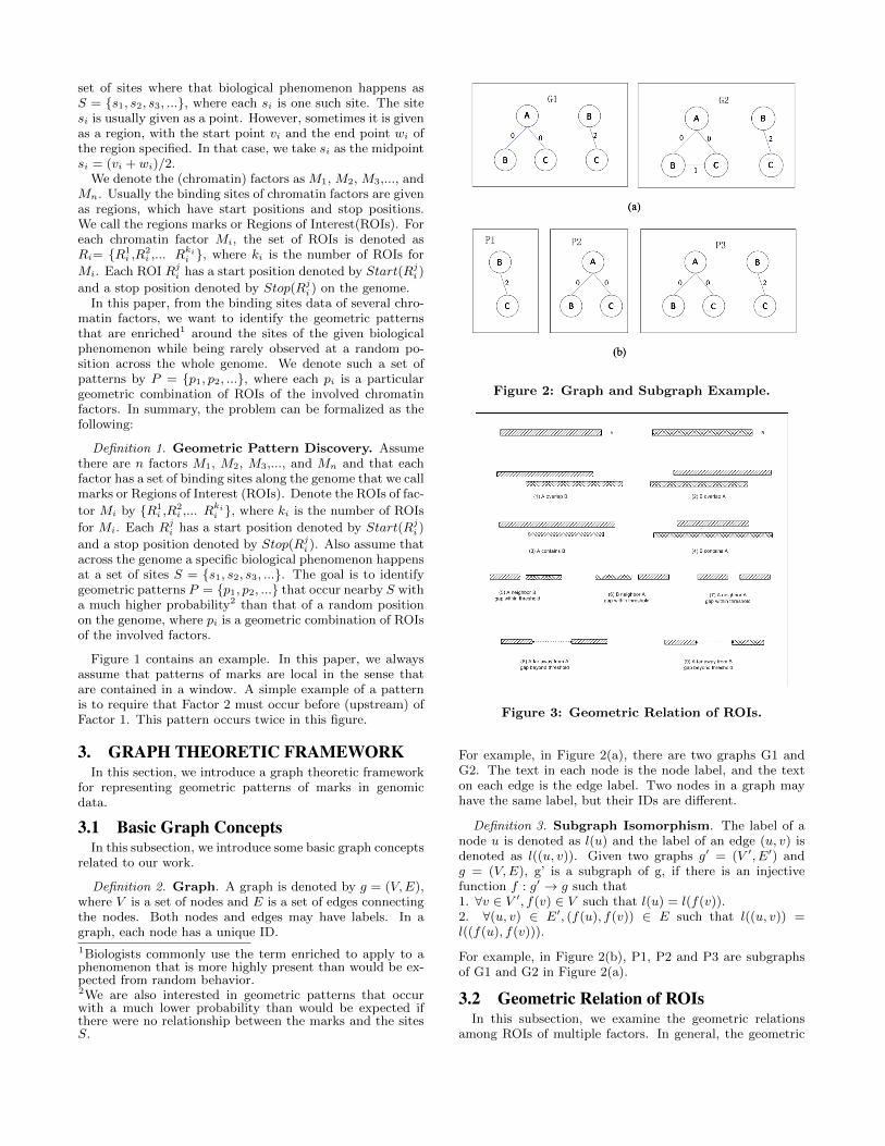
Figure 2: Graph and Subgraph Example.

Figure 3: Geometric Relation of ROIs.

For example, in Figure 2(a), there are two graphs G1 andG2. The text in each node is the node label, and the texton each edge is the edge label. Two nodes in a graph mayhave the same label, but their IDs are di↵erent.

Definition 3. Subgraph Isomorphism. The label of anode u is denoted as l(u) and the label of an edge (u, v) isdenoted as l((u, v)). Given two graphs g0 = (V 0, E0) andg = (V,E), g’ is a subgraph of g, if there is an injectivefunction f : g0 ! g such that1. 8v 2 V 0, f(v) 2 V such that l(u) = l(f(v)).2. 8(u, v) 2 E0, (f(u), f(v)) 2 E such that l((u, v)) =l((f(u), f(v))).

For example, in Figure 2(b), P1, P2 and P3 are subgraphsof G1 and G2 in Figure 2(a).

3.2 Geometric Relation of ROIsIn this subsection, we examine the geometric relations

among ROIs of multiple factors. In general, the geometric

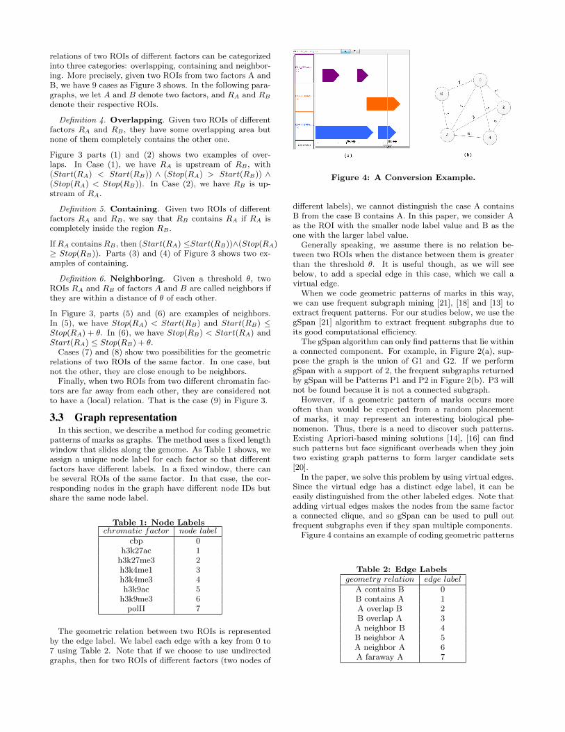
relations of two ROIs of di↵erent factors can be categorizedinto three categories: overlapping, containing and neighbor-ing. More precisely, given two ROIs from two factors A andB, we have 9 cases as Figure 3 shows. In the following para-graphs, we let A and B denote two factors, and RA and RB

denote their respective ROIs.

Definition 4. Overlapping. Given two ROIs of di↵erentfactors RA and RB , they have some overlapping area butnone of them completely contains the other one.

Figure 3 parts (1) and (2) shows two examples of over-laps. In Case (1), we have RA is upstream of RB , with(Start(RA) < Start(RB)) ^ (Stop(RA) > Start(RB)) ^(Stop(RA) < Stop(RB)). In Case (2), we have RB is up-stream of RA.

Definition 5. Containing. Given two ROIs of di↵erentfactors RA and RB , we say that RB contains RA if RA iscompletely inside the region RB .

IfRA containsRB , then (Start(RA) Start(RB))^(Stop(RA)� Stop(RB)). Parts (3) and (4) of Figure 3 shows two ex-amples of containing.

Definition 6. Neighboring. Given a threshold ✓, twoROIs RA and RB of factors A and B are called neighbors ifthey are within a distance of ✓ of each other.

In Figure 3, parts (5) and (6) are examples of neighbors.In (5), we have Stop(RA) < Start(RB) and Start(RB) Stop(RA) + ✓. In (6), we have Stop(RB) < Start(RA) andStart(RA) Stop(RB) + ✓.

Cases (7) and (8) show two possibilities for the geometricrelations of two ROIs of the same factor. In one case, butnot the other, they are close enough to be neighbors.

Finally, when two ROIs from two di↵erent chromatin fac-tors are far away from each other, they are considered notto have a (local) relation. That is the case (9) in Figure 3.

3.3 Graph representationIn this section, we describe a method for coding geometric

patterns of marks as graphs. The method uses a fixed lengthwindow that slides along the genome. As Table 1 shows, weassign a unique node label for each factor so that di↵erentfactors have di↵erent labels. In a fixed window, there canbe several ROIs of the same factor. In that case, the cor-responding nodes in the graph have di↵erent node IDs butshare the same node label.

Table 1: Node Labelschromatic factor node label

cbp 0h3k27ac 1h3k27me3 2h3k4me1 3h3k4me3 4h3k9ac 5h3k9me3 6polII 7

The geometric relation between two ROIs is representedby the edge label. We label each edge with a key from 0 to7 using Table 2. Note that if we choose to use undirectedgraphs, then for two ROIs of di↵erent factors (two nodes of

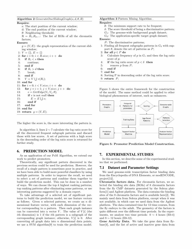
Figure 4: A Conversion Example.

di↵erent labels), we cannot distinguish the case A containsB from the case B contains A. In this paper, we consider Aas the ROI with the smaller node label value and B as theone with the larger label value.

Generally speaking, we assume there is no relation be-tween two ROIs when the distance between them is greaterthan the threshold ✓. It is useful though, as we will seebelow, to add a special edge in this case, which we call avirtual edge.

When we code geometric patterns of marks in this way,we can use frequent subgraph mining [21], [18] and [13] toextract frequent patterns. For our studies below, we use thegSpan [21] algorithm to extract frequent subgraphs due toits good computational e�ciency.

The gSpan algorithm can only find patterns that lie withina connected component. For example, in Figure 2(a), sup-pose the graph is the union of G1 and G2. If we performgSpan with a support of 2, the frequent subgraphs returnedby gSpan will be Patterns P1 and P2 in Figure 2(b). P3 willnot be found because it is not a connected subgraph.

However, if a geometric pattern of marks occurs moreoften than would be expected from a random placementof marks, it may represent an interesting biological phe-nomenon. Thus, there is a need to discover such patterns.Existing Apriori-based mining solutions [14], [16] can findsuch patterns but face significant overheads when they jointwo existing graph patterns to form larger candidate sets[20].

In the paper, we solve this problem by using virtual edges.Since the virtual edge has a distinct edge label, it can beeasily distinguished from the other labeled edges. Note thatadding virtual edges makes the nodes from the same factora connected clique, and so gSpan can be used to pull outfrequent subgraphs even if they span multiple components.

Figure 4 contains an example of coding geometric patterns

Table 2: Edge Labelsgeometry relation edge label

A contains B 0B contains A 1A overlap B 2B overlap A 3A neighbor B 4B neighbor A 5A neighbor A 6A faraway A 7

of marks as graphs. Figure 4(a) shows a view of 3 chromatinfactors between 248500 and 252000 on fly chromosome 2Lusing visualization tool GeneBrowser [3]. In this figure, eachrow gives the binding sites for a chromatin factor: row 1 forthe factor cbp, row 2 for h3k4me1, and row 3 for h3k4me3.Their node labels are given in Table 1. Using the edge labelsgiven in Table 2, we get Figure 4(b) as the graph represen-tation for the window from 248500 to 252000 in Figure 4(a).In Figure 4(a), there are 2 ROIs of cbp, 1 ROI of h3k4me1,and 2 ROIs of h3k4me3 in the window. This gives 5 nodesin the graph representation. There is one virtual edge inthe graph and its edge label is 7. Note that it is not nec-essary for an ROI to be completely included in the windowto be considered as a node. As long as part of the ROI isin the window, we create a node. Although h3k4me1 andh3k4me3 are cut o↵ by the boundary of the window, theyare still represented in the graph in Figure 4(b).

The representation is quite flexible and we can simplychange the definition of node labels and edge labels to adaptto various applications. If we would like to include more fac-tors for the application, we can define some new node labels.If we do not want to di↵erentiate between overlapping andcontaining, we can set their edge labels to the same value.

3.4 Framework of proposed approachOnce the graph is formed, it is straightforward to extract

the geometric patterns of marks. Here are the steps:

1. Step 0: Generate the genome-wide background graphdataset G1 from the marks.

2. Step 1: Add the locations of the phenomenon of biolog-ical interest to create application-specific target graphdataset G2.

3. Step 2: Given a support s, find all frequent patternsin G2, denoted by P = {p1, p2, ...}.

4. Step 3: For each pi in P , calculate its frequency in G1

as well as its log ratio score and sort P in descendingorder.

5. Step 4: Analyze the patterns having high log ratioscores.

4. GRAPH GENERATION ALGORITHMIn this section, we describe the PoM Algorithm for gener-

ating graph datasets from the ROIs data of di↵erent chro-matin factors across the genome.Algorithm 1 describes the Graph Generating Algorithm.

Lines 2 ⇠ 8 generate the genome-wide background datasetand lines 9 ⇠ 15 generate the phenomenon-oriented targetgraph dataset. In the algorithm, the size and step of thesliding window are controllable and can be adjusted by theuser for di↵erent needs.Given the start position s and an end position d, the Gen-

erateOneSlidingGraph Algorithm generates the graph repre-sentation for the factors falling within the region [s, d]. Lines2 ⇠ 10 add all the factors within[s, d] as nodes in the graph,and lines 11 ⇠ 18 check every pair of nodes and add thecorresponding edges. The algorithm returns null for emptygraphs. The GetEdge function checks the geometric rela-tion of two nodes and returns the corresponding edge withthe proper label. It returns null for two faraway ROIs ofdi↵erent chromatin factors.

Algorithm 1 PoM Graph Generation Algorithm.

Require:size: The length of a sliding window;step: How far to slide the moving window;n: The length of the whole genome;✓: Neighboring threshold;R: The set of ROIs of all the chromatin factors;S: The set of sites where the biological phenomenon hap-pens;

Ensure:G1: Genome-wide background graph dataset;G2: application-specific target graph dataset;

1: G1 = {}, G2 = {}2: Sorting R in the ascending order of the start position.3: for i = 0; i ⇤ step < n; i++ do4: gi = GenerateOneSlidingGraph(i ⇤ step, i ⇤ step +

size, ✓, R);5: if gi is not null then6: G1 = G1

Sgi

7: end if8: end for9: for all p 2 S do10: c = The centroid of p;11: g0 = GenerateOneSlidingGraph(c � size/2, c +

size/2, ✓, R);12: if g0 is not null then13: G2 = G2

Sg0;

14: end if15: end for16: return G1, G2;

5. SIGNIFICANT PATTERNS MININGIn this section, we describe how to find out the significant

geometric patterns after generating the graph. The methodis presented in algorithm 3.

It is important to sort by significance the frequent sub-graphs produced. Since our interest is in geometric patternsof marks that occur relatively frequently over biological phe-nomena of interest, but relatively rarely otherwise, we intro-duce a score to quantify this. The score function is definedbased on the pattern’s positive frequency and backgroundfrequency.

Definition 7. Positive frequency. The positive frequencyfp(p) of a subgraph pattern p is the ratio of the number oftarget graphs containing p to the total number of targetgraphs.

Definition 8. Background frequency. The backgroundfrequency fb(p) of a subgraph pattern p is the ratio of thenumber of background graphs (i.e. graphs that are not overa region representing a phenomenon of biological interest)containing p to the total number of background graphs.

Definition 9. Log ratio score. The log ratio score of asubgraph pattern p is the log ratio of the positive frequencyto the background frequency of p and is defined as:

log ratio score of pattern p = logfp(p)fb(p)

The log ratio score is used to estimate the interest of thepattern pi. A high log ratio score means the pattern has amuch higher chance to be present over phenomena of biolog-ical interest compared to a random place along the genome.

Algorithm 2 GenerateOneSlidingGraph(s, d, ✓, R)

Require:s: The start position of the current window;d: The end position of the current window;✓: Neighboring threshold;R = R1,R2,...: The list of ROIs of all the chromatinfactors;

Ensure:g = (V,E): the graph representation of the current slid-ing window;

1: V = {}, E = {}2: for i = 0; i < R.size; i++ do3: if Ri < s then4: continue;5: end if6: if Ri > d then7: break;8: end if9: V = V

Sv(Ri);

10: end for11: for i = 0; i < V.size; i++ do12: for j = i+ 1; j < V.size; j ++ do13: e = GetEdge(Vi, Vj , ✓);14: if e is not null then15: E = E

Se;

16: end if17: end for18: end for19: return g = (V,E);

The higher the score is, the more interesting the pattern is.

In algorithm 3, lines 2 ⇠ 7 calculate the log ratio score forall the discovered frequent subgraph patterns and discardthose with low scores. A set of patterns with a high scorein the descending order of the log ratio score is returned forfurther study.

6. PREDICTION MODELAs an application of our PoM Algorithm, we extend our

work to predict promoters.Theoretically, any significant pattern discovered in the

previous section could be used for prediction. However, therecall of a single pattern is sometimes poor in practice, andwe have been able to build more powerful classifiers by usingmultiple patterns. In order to improve the recall, we needto select a set of patterns and combine them together tobuild the prediction model. This can be done in a numberof ways. We can choose the top k highest ranking patterns,top ranking patterns after eliminating some patterns, or useinteresting patterns suggested by a domain expert.

To take advantage of a selected set of significant pat-terns to build the prediction model, we use feature vectorsas follows. Given n selected patterns, we create an n di-mensional feature vector, with each dimension of the vec-tor corresponding to a pattern. Then each graph instancecan be converted into a vector V . The value of V [i] (theith dimension) is 1 if the ith pattern is a subgraph of thecorresponding graph instance; otherwise, V [i] is 0. Afterconverting all graph data into n dimensional data points,we use a SVM algorithm[9] to train the prediction model.

Algorithm 3 Pattern Mining Algorithm .

Require:✓: The minimum support rate to be frequent;�: The score threshold of being a discriminative pattern;G1: The genome-wide background graph dataset;G2: The application-specific target graph dataset;

Ensure:P : The discriminative patterns;

1: Finding all frequent subgraphs patterns in G2 with sup-port ✓, denote the set of patterns as P ;

2: for all p 2 P do3: Calculate frequency of p in G1 and then the log ratio

score of p;4: if the log ratio score of p < � then5: remove p from P ;6: end if7: end for8: Sorting P in descending order of the log ratio score.9: return P ;

Figure 5 shows the entire framework for the constructionof the model. The same method could be applied to otherbiological phenomenon of interest, such as enhancers.

Figure 5: Promoter Prediction Model Construction.

7. EXPERIMENTAL STUDIESIn this section, we describe some of the experimental stud-

ies that we performed.

7.1 Dataset and Parameter SettingsWe used genome-wide transcription factor binding data

from the Encyclopedia of DNA Elements, or modENCODE,project[12].Chromatin factors data. For chromatin factors, we se-lected the binding site data (ROIs) of 8 chromatin factorsfrom the fly ChIP datasets generated by the Solexa plat-form[1] and Agilent platform. The data contains the bindingsites of the 8 chromatin factors and is available here[2]. Wemainly used data from Solexa platform, except when it wasnot available, in which case we used data from the Agilentplatform. The data contained time for 12 time courses, fromthe fly embryo to the adult. The geometry of the factors isquite di↵erent over the di↵erent time periods. In the exper-iments, we analyze two time periods: 0 ⇠ 4 hours (E0-4)and 8 ⇠ 12 hours (E8-12).Gene Activity Data. We take the gene data from fly-base[4], and the list of active and inactive gene data from

[12]. For the embryo 0 ⇠ 4 hours, we have 9657 active genesand 9169 inactive genes.

Table 3: Promoter Graph Datatime course promoter graphs genomewide graphs

E0-4 5484 49056E8-12 5245 40384

Table 4: Promoter Classification DataE0-4 Positive Negative

Training data 3630 4200Testing data 1854 2202

E8-12 Positive NegativeTraining data 3470 4000Testing data 1765 2000

Promoter Data. The analysis of the promoter dataset isshown in Tables 3 and 4. Table 3 shows the graph statisticsand Table 4 gives the data used for classification. For thepurpose of classification, we need both positive cases andnegative cases. We assume that the sites where promotersoccur are positive cases and the sites without promoters arenegative cases. We extract the promoters from the Tran-scription Start Site (TSS) class annotation at FDR 0.05, inthe Supplementary Table 6 in [12]. This data gives the lo-cation information of the known promoters. We take theactive promoters marked with “TP” and “FN” in that table.For each active promoter, we simply generate a graph basedon its location. Then we randomly split the data into twogroups, one for training and the other for testing.

Negative cases are generated by random drawing on agenome-wide basis. We randomly pick a region and use it asa negative instance if there is no TSS within 2000 base pairs.The negative cases are divided into two groups as well.

We have to choose carefully the size of the sliding window.On the one hand, if the window size is too small, it will notcapture the geometry of di↵erent factors. On the other hand,if it is too large, the graph produced will be too complicated.The size of ROIs varies a lot for di↵erent chromatin factors.Some tend to have ROIs larger than 10,000 base pairs, whileothers are more likely to have ROIs of several hundred basepairs. In our experiments, we set the window size as 2000base pairs. The sliding step is set to 1000 base pairs sothat the two neighboring windows have 1000 base pairs ofoverlapping area.

In the experiments, to simplify the analysis, we use thesame edge label for cases 1 to 4 in Figure 3. Table 1 is usedto label the nodes. When mining the frequent patterns forthe gene activity graphs, we set the minimum support tobe 5%. For promoter prediction, we tried multiple supportvalues. We selected a threshold log ratio score of 0.7.

7.2 Gene ActivityIn this set of experiments, we take the chromatin factors

data of embryo 0 ⇠ 4 hours. We performed two sets ofexperiments on the above dataset. In the first set of exper-iments, we take the graphs of the active genes as the targetdataset and graphs of the inactive genes as the backgrounddataset. The top four discriminative patterns are shown inFigure 6, and their scores are shown in Table 5.

Figure 6: Active Patterns.

We can see that two h3k4me3s occur in all those 4 pat-terns, which indicates that the h3k4me3 has a positive im-pact on the gene expression. This is confirmed by the bi-ological observations: h3k4me3 is an important epigeneticlandmark for active transcription [15] [12].

In the second set of experiments, we take the graphs of theinactive genes as the target dataset and graphs of the activegenes as the background dataset. The most discriminativepattern found is shown in Figure 7, and its score is shownin Table 6.

Figure 7: Inactive Pattern.

Table 5: Statistics of Active PatternsID # in G2 # in G1 fp fb ratio score1 512 13 7.32% 0.91% 8.07 0.9072 471 12 6.74% 0.84% 8.05 0.9053 390 10 5.58% 0.70% 8.0 0.9024 761 22 10.89% 1.54% 7.09 0.851

The result indicates that h3k9me3 and h3k27me3 togethercan repress the gene expression. This is in accordance withthat h3k9me3 and h3k27me3 are often found associated withrepressed genes for multiple species [17] [7].

7.3 Promoter Prediction

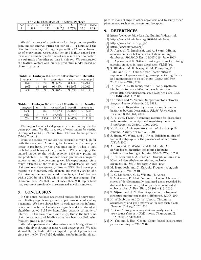
Table 6: Statistics of Inactive PatternID # in G2 # in G1 fp fb ratio score1 382 122 26.7% 1.75% 15.3 1.184

We did two sets of experiments for the promoter predic-tion, one for embryo during the period 0 ⇠ 4 hours and theother for the embryo during the period 8 ⇠ 12 hours. In eachset of experiments, we reduced the top k highest ranked pat-terns into a smaller pattern set of size n such that no patternis a subgraph of another pattern in this set. We constructedthe feature vectors and built a predictive model based onthose n patterns.

Table 7: Embryo 0-4 hours Classification Resultssupport n k precision recall accuracy15% 15 72 93.53% 83.44% 89.79%10% 17 197 93.47% 84.20% 90.09%5% 23 893 93.62% 83.87% 90.01%

Table 8: Embryo 8-12 hours Classification Resultssupport n k precision recall accuracy15% 10 84 97.12% 84.02% 91.34%10% 13 313 97.49% 83.74% 91.37%5% 26 1908 97.33% 84.65% 91.71%

The support is a critical parameter when mining the fre-quent patterns. We did three sets of experiments by settingthe support as 5%, 10% and 15%. The results are given inTables 7 and 8.

From the tables, we can see the precision is very high forboth time courses. According to the results, if a new pro-moter is predicted by the prediction model, it has a highprobability of being a true promoter. When we apply thetrained model to the whole genome, 1859 new promotersare predicted. To fully validate these predictions, requiresexpensive and time consuming wet lab experiments. As arough estimate of the validity of our predictions, we notethat promoters are generally close to TSS. For known pro-moters in our dataset, 99% of them are within 2000 bp of aTSS. Among the new predicted promoters, 91% of them arewithin 2000 bp of a TSS, which is highly encouraging. Fur-thermore, even 9% that do not meet their 2000 bp criteriamay represent previously unrecognized novel promoters.

8. CONCLUSIONIn this paper, we have abstracted and studied a new prob-

lem: finding significant geometric patterns of marks alonga genome. We have shown how to code geometric informa-tion about patterns of marks as a graph and introduced analgorithm called PoM for identifying patterns of marks ofinterest. To the best of our knowledge, this is the first timethat the geometry of binding sites has been studied usingfrequent graph algorithms.

We did experimental studies using the PoM algorithm tostudy the fly’s chromatin factors and active genes. We alsoshowed the method could be adapted to predict promoter re-gions for the fly. The PoM algorithm can be immediately ap-

plied without change to other organisms and to study otherphenomena, such as enhancers and hotspots.

9. REFERENCES[1] http://genepool.bio.ed.ac.uk/illumina/index.html.[2] http://www.bionimbus.org:8080/bionimbus/.[3] http://www.bioviz.org/igb/.[4] http://www.flybase.org/.[5] R. Agrawal, T. Imielinski, and A. Swami. Mining

association rules between sets of items in largedatabases. SIGMOD Rec., 22:207–216, June 1993.

[6] R. Agrawal and R. Srikant. Fast algorithms for miningassociation rules in large databases. VLDB ’94.

[7] S. Bilodeau, M. H. Kagey, G. M. Frampton, P. B.Rahl, and R. A. Young. Setdb1 contributes torepression of genes encoding developmental regulatorsand maintenance of es cell state. Genes and Dev.,23(21):2484–2489, 2009.

[8] D. Chen, A. S. Belmont, and S. Huang. Upstreambinding factor association induces large-scalechromatin decondensation. Proc Natl Acad Sci USA,101:15106–15111, 2004.

[9] C. Cortes and V. Vapnik. Support-vector networks.Support-Vector Networks, 20, 1995.

[10] E. B. et al. Regulation by transcription factors inbacteria: beyond description. FEMS Microbiologyreviews, 33:133–151, 2009.

[11] F. T. et al. Flynet: a genomic resource for drosophilamelanogaster transcriptional regulatory networks.Bioinformatics, 25:3001–3004, 2009.

[12] N. N. et al. A cis-regulatory map of the drosophilagenome. Nature, 471:527–531, 2011.

[13] J. Huan, W. Wang, and J. Prins. E�cient mining offrequent subgraphs in the presence of isomorphism.ICDM, 2003.

[14] A. Inokuchi, T. Washio, and H. Motoda. Anapriori-based algorithm for mining frequentsubstructures from graph data. ECML PKDD, 2000.

[15] H. H. Kavi and J. A. Birchler. Drosophila kdm2 is ah3k4me3 demethylase regulating nucleolarorganization. BMC Research Notes, 2009.

[16] M. Kuramochi and G. Karypis. Frequent subgraphdiscovery. ICDM, 2001.

[17] L. C. Lindeman, C. L. Winata, H. Aanes,S. Mathavan, P. Alestrom, and P. Collas. Chromatinstates of developmentally-regulated genes revealed bydna and histone methylation patterns in zebrafishembryos. Int. J. Dev. Biol., 54:803 – 813, 2010.

[18] S. Nijssen and J. N. Kok. A quickstart in frequentstructure mining can make a di↵erence. KDD, 2004.

[19] H. Willenbrock and D. W. Ussery. Chromatinarchitecture and gene expression in escherichia coli.Genome Biology, 5:252, 2004.

[20] X. Yan. Mining, indexing and similarity search inlarge graph data sets. PhD thesis, Champaign, IL,USA, 2006. AAI3243031.

[21] X. Yan and J. Han. Gspan: Graph-based substructurepattern mining. ICDM, 2002.