Discount rates and employment fluctuations

Jaroslav Borovicka

New York University

jaroslav.borovicka@nyu.edu

Katarına Borovickova

New York University

katarina.borovickova@nyu.edu

September 27, 2017

Preliminary draft.

Abstract

We study the role of fluctuations in discount rates for the joint dynamics of expected

returns in the stock market and employment dynamics. We construct a non-parametric

bound on the predictability and time-variation in conditional volatility of the firm’s

profit flow that must be met to rationalize the observed business-cycle fluctuations in

hiring. A stochastic discount factor consistent with conditional moments of the risk-

free rate and expected returns on risky assets alleviates the need for an excessively

volatile model of the expected profit flow.

1 Introduction

Stock market valuation and the dynamics of labor market variables are highly volatile relative

to conventional measures of macroeconomic risk and strongly correlated with the business

cycle, while the real risk-free rate is smooth. The volatility in the stock market variables

in excess of the subsequent movements in dividends is the basis of the Shiller (1981) excess

volatility puzzle in the asset pricing literature. On the other hand, Shimer (2005) identi-

fied the discrepancy between the volatility in labor market tightness and measures of labor

productivity as an excess volatility puzzle in search and matching models of the labor market.

Campbell and Shiller (1988) and the subsequent literature use linear approximations of

present value budget constraints to argue that variation in price-dividend ratios unexplained

by movements in subsequent dividends have to be attributed to fluctuations of discount rates

applied to these dividends. However, given the smoothness of yields on risk-free assets, in

particular the real risk-free rate, this fluctuation in discount rates has to come mainly in

the form of time-varying compensation for risk, manifested in fluctuations in the conditional

volatility of the stochastic discount factor.

The search and matching literature dealt with the Shimer (2005) puzzle by introducing

mechanisms that increase the volatility and cyclicality of the profit flow received by the firm

from hiring the marginal worker (Hall and Milgrom (2008), Hagedorn and Manovskii (2008),

Christiano et al. (2015), and others). However, the preferences used in these papers imply

minimal compensations for risk, which are not able to rationalize standard asset pricing facts

including large risk premia for risky cash flows and fluctuations in the valuation of the stock

market.

In this paper, we provide a quantitative connection between these economic forces through

business cycle fluctuations in discount rates that investors and firms use to discount future

risky cash flows. In particular, we construct a non-parametric bound on two moments of

firm’s profit dynamics that emerges from the optimality condition on firm’s hiring.

One of the moments is the volatility of the conditional expectation of firm’s profits. The

standard approach in the search and matching literature dictates to make this volatility high,

so that business-cycle fluctuations in expected profits are able to explain changes in incentives

of firms to hire workers. The other moment is the average conditional volatility of the profit

flow. Business cycle fluctuations in the conditional volatility of innovations to profits that

are correlated with innovations to the stochastic discount factor lead to fluctuations in risk

premia associated with the firm’s profit flow and again generate procyclical incentives to hire

workers.

The bound that we construct reveals that a successful model of the labor market dy-

1

namics that relies on the optimality condition for hiring must satisfy this condition through

a combination of the above two channels. Introducing a properly modeled stochastic dis-

count factor than alleviates the burden imposed by the optimality condition on generating

an excessively volatile expected profit flow, and allows to shift part of the weight on the risk

compensation channel. This approach has been effectively followed by some of the recent

work in the asset pricing literature (Petrosky-Nadeau et al. (2015), Favilukis and Lin (2016),

Kuehn et al. (2014) Favilukis et al. (2015), Belo et al. (2014), Donangelo et al. (2016), Kilic

and Wachter (2015) and others).

We then direct our attention to modeling these risk compensations using structural re-

strictions on the form of the stochastic discount factor. We endow a representative investor

with recursive preferences introduced by Epstein and Zin (1989, 1991). In order to allow for

fluctuations in risk compensation, we allow the risk aversion parameter in the preferences

to be time varying. While this adds flexibility to the preference structure, we discipline the

time-variation in the risk aversion parameter by making it consistent with the dynamics of

the equity premium in the economy. We call the innovations to the risk aversion parameter

discount rate shocks.

Finally, we use the inferred stochastic discount factor to price cash flows that firms

receive. We model firms as operating in a labor market with search and matching frictions.

Firms incur cost of post vacancies that are necessary to hire workers. In equilibrium with

free entry, the cost of vacancy posting has to be equal to the value of a job to the firm,

given by the present discounted value of the surplus the firm earns from hiring a marginal

worker. Fluctuations in the value of the job lead to time-variation in incentives of firms to

hire workers, and hence to fluctuations in employment. In the environment, we quantify the

contribution of discount rate shocks to the fluctuations in the labor market variables.

Our paper is not the first to consider discount rates as a plausible explanation. Perhaps

the closest paper to ours is Hall (2017), who highlights the economic forces that discount

rate shocks play in the search and matching framework, and provides valuable insights into

the interactions between the stochastic discount factor and profit flow. However, his model

of preferences implies that most of the time-variation in discount rates is manifested as time-

variation in the mean, as opposed to the dispersion, of the stochastic discount factor, and

hence implies quantitatively implausible movements in the risk-free rate.

2 Theoretical framework

We consider a discrete-time environment with optimizing investors in financial markets and

firms hiring workers in a frictional labor market. In this environment, optimality conditions

2

are described by two types of forward-looking restrictions. In the financial market, these

restrictions have the form of Euler equations for the valuation of returns on alternative

assets. In the labor market, optimal choice of hiring implies an intertemporal condition that

equalizes the cost of hiring the marginal worker with the present discounted value of profits

generated by employing this worker. We then introduce a criterion that will be useful for

the characterization of profit flow processes consistent with this intertemporal condition.

2.1 Restrictions

Investors have unconstrained access to a vector of n securities with one-period real returns

Rit+1, i = 1, . . . , n. Investor optimization and absence of arbitrage imply that there exists a

stochastic discount factor process St such that

Et

[st+1R

it+1

]= 1, i = 1, . . . , n. (1) {eq:EsR}

where st+1.= St+1/St is the investors’ marginal rate of substitution.

Firms in the production sector hire workers in a Diamond–Mortensen–Pissarides labor

market. Firms post vacancies at a per-period cost κ, and the vacancies are filled at an

equilibrium rate qt. Free entry and optimal hiring choice imply that the value to the firm of

hiring a marginal worker must be equal to the expected cost of hiring the marginal worker,

κ/qt. This implies the Euler equation

κ

qt= Et [st+1πt+1] + Et

[st+1 (1− δt+1)

κ

qt+1

](2) {eq:hiring_Euler_equation

where πt+1 is the firm’s profit flow from the marginal worker, and δt+1 the probability of

match separation. The equation dictates that observed fluctuations in vacancy filling rates

qt and separation rates δt+1 have to be rationalized through fluctuations in firms’ marginal

profit flow πt+1 and the stochastic discount factor st+1. In expansions, the vacancy filling

rate qt is low, and hence Et [st+1πt+1] needs to be high. Writing the expected profit flow as

Et [st+1πt+1] = Et [st+1]Et [πt+1] + Covt (st+1, πt+1) (3) {eq:Espi}

uncovers three sources of variation. When agents are risk-neutral, as in much of the search

and matching literature, we have st+1 = β and observed differences in vacancy filling rates

must be rationalized through fluctuations in firm’s expected profits Et [πt+1]. In a more

general environment, fluctuations in the conditional mean of the stochastic discount factor

Et [st+1] and time-variation in the covariance Covt (st+1, πt+1) contribute to the variation in

3

expected discounted profit flow as well.

Our goal is to provide a stochastic discount factor that is consistent with evidence on

cross-sectional differences and time-variation in expected returns, and use it to infer charac-

teristics of a class of processes πt that are consistent with optimal hiring choice (2). Denoting

gt+1 =κ

qt− st+1 (1− δt+1)

κ

qt+1(4) {eq:g_expression

we have

0 = Et [st+1πt+1 − gt+1]

In order to empirically implement the conditional restriction (2), we instrument the equation

as in Hansen and Singleton (1982) with a vector of variables zπt , and get

0 = E [zπt (st+1πt+1 − gt+1)] . (5) {eq:Espi_instrumented

The vector of instruments zπt contains business cycle variables that serve as predictors of

future state of the labor market. Equation (5) states that the Euler equation errors st+1πt+1−

gt+1 are not systematically related to these predictors.

We proceed in an analogous fashion with the vector of asset pricing restrictions (1), using

a vector of instruments zst . This implies the set of restrictions1

0 = E[zst(st+1R

it+1 − 1

)], i = 1, . . . n. (6) {eq:EsR_instrumented

2.2 Objective

There will typically be many processes πt consistent with the set of restrictions (5), and both

theoretical modeling as well as empirical measurement of πt are challenging. Theory dictates

that the Euler equation (2) holds for the profit flow associated with the marginal worker

but this profit flow is not directly obtainable from data. The theoretical literature then

frequently sidesteps this issue by introducing environments where the average and marginal

workers are identical.

Rather than explicitly modeling the profit flow, we aim at asking what are the minimal

requirements that every profit flow process consistent with (2) must satisfy. Since the liter-

ature has traditionally struggled to generate profit processes that are sufficiently volatile to

rationalize fluctuations in the vacancy filling rates, we are looking for the lower bound on

1We can write this set of restrictions in concise form as 0 = E [zst ⊗ (st+1Rt+1 − 1)] where ⊗ is the

Kronecker product and 1 is a column vector of ones of length n. For two column vectors x =(xi)ki=1

and

y =(yj)nj=1

, x⊗ y is a column vector of length k × n with (x⊗ y)(i−1)n+j

= xiyj .

4

dispersion of the profit process for (5) to hold.

Since we can write (3) as

Et [st+1πt+1] = Et [st+1]Et [πt+1] + ρt (st+1, πt+1)σt (st+1)σt (πt+1)

where ρt is the conditional correlation and σt the conditional standard deviation, the two

key moments that can offset fluctuations in qt are Et [πt+1] and σt (πt+1). This motivates the

objective

Lα = αV ar [Et [πt+1]] + (1− α)E [V art [πt+1]]

As a function of α, this objective generates a lower bound on the combinations of variance

of the conditional mean and average conditional variance of the profit process such that

it is consistent with the restrictions above. When α = 12, then the objective is equal to

12V ar [πt+1]. The objective Lα can therefore be thought of as a generalization of the Law of

Total Variance.

When αց 0, the objective emphasizes the minimization of average conditional variance

E [V art [πt+1]]. Then, in order to rationalize (2), the process πt has to become highly pre-

dictable and exhibit large fluctuations in the conditional mean Et [πt+1]. This is the only

way how to resolve the unemployment volatility puzzle when st+1 = β.

On the other hand, when α ր 1, the objective Lα stresses the minimization of the varia-

tion in Et [πt+1]. From equation (3), we infer that the resolution of the unemployment volatil-

ity puzzle must arise from sufficiently large business cycle fluctuations in Covt (st+1, πt+1).

These can emerge from sufficiently large fluctuations in the conditional volatility of the

stochastic discount factor but if these are not large enough, conditional volatility of the

profit process will have to fluctuate as well.

3 Bounds

For a given model of a stochastic discount factor and data on separation rates and vacancy

filling probabilities, the problem is

minπt+1

Lα subject to 0 = E [zπt (st+1πt+1 − gt+1)] . (7) {eq:profit_bound_problem

When α = 12, the problem reduces to finding the minimum variance profit process, and the

solution corresponds to the lowest point on the Hansen and Jagannathan (1991) bound.

5

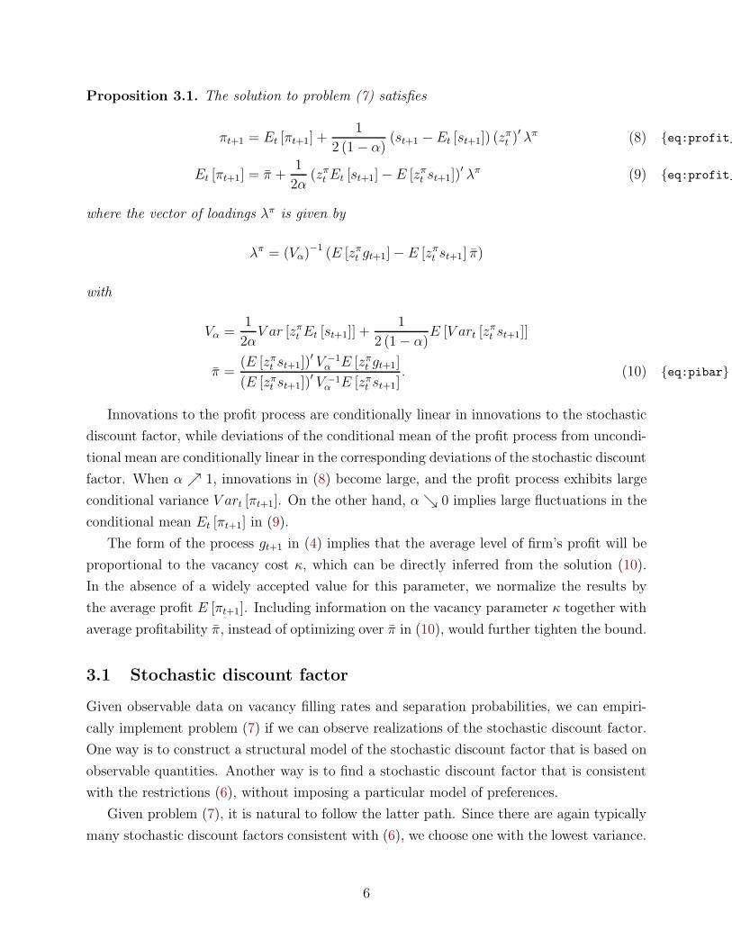
Proposition 3.1. The solution to problem (7) satisfies

πt+1 = Et [πt+1] +1

2 (1− α)(st+1 − Et [st+1]) (z

πt )

′ λπ (8) {eq:profit_bound_solution1

Et [πt+1] = π +1

2α(zπt Et [st+1]− E [zπt st+1])

′ λπ (9) {eq:profit_bound_solution2

where the vector of loadings λπ is given by

λπ = (Vα)−1 (E [zπt gt+1]− E [zπt st+1] π)

with

Vα =1

2αV ar [zπt Et [st+1]] +

1

2 (1− α)E [V art [z

πt st+1]]

π =(E [zπt st+1])

′ V −1α E [zπt gt+1]

(E [zπt st+1])′ V −1

α E [zπt st+1]. (10) {eq:pibar}

Innovations to the profit process are conditionally linear in innovations to the stochastic

discount factor, while deviations of the conditional mean of the profit process from uncondi-

tional mean are conditionally linear in the corresponding deviations of the stochastic discount

factor. When α ր 1, innovations in (8) become large, and the profit process exhibits large

conditional variance V art [πt+1]. On the other hand, αց 0 implies large fluctuations in the

conditional mean Et [πt+1] in (9).

The form of the process gt+1 in (4) implies that the average level of firm’s profit will be

proportional to the vacancy cost κ, which can be directly inferred from the solution (10).

In the absence of a widely accepted value for this parameter, we normalize the results by

the average profit E [πt+1]. Including information on the vacancy parameter κ together with

average profitability π, instead of optimizing over π in (10), would further tighten the bound.

3.1 Stochastic discount factor

Given observable data on vacancy filling rates and separation probabilities, we can empiri-

cally implement problem (7) if we can observe realizations of the stochastic discount factor.

One way is to construct a structural model of the stochastic discount factor that is based on

observable quantities. Another way is to find a stochastic discount factor that is consistent

with the restrictions (6), without imposing a particular model of preferences.

Given problem (7), it is natural to follow the latter path. Since there are again typically

many stochastic discount factors consistent with (6), we choose one with the lowest variance.

6

This stochastic discount factor is obtained by solving

minst+1

1

2E[(st+1 − E [st+1])

2] subject to 0 = E[zst(st+1R

it+1 − 1

)], i = 1, . . . n. (11) {eq:SDF_bound_problem

The variance-minimizing stochastic discount factor lies at the lowest point of the Hansen–

Jagannathan bound and the solution has a structure analogous to that for the profit process

πt+1 in Proposition 3.1.2

Proposition 3.2. The minimum-variance stochastic discount factor that solves problem (11)

is given by

st+1 = s+ (zst ⊗Rt+1 −E [zst ⊗Rt+1])′ λs

where the vector of loadings λs and the mean of the stochastic discount factor are

λs = (V ar [zst ⊗ Rt+1])−1 (E [zst ]−E [zst ⊗Rt+1] s)

s =(E [zst ⊗ Rt+1])

′ (V ar [zst ⊗ Rt+1])−1E [zst ]

(E [zst ⊗ Rt+1])′ (V ar [zst ⊗ Rt+1])

−1E [zst ⊗ Rt+1].

The stochastic discount factor is therefore a conditionally linear function of returns, and

variation in instruments serves as fluctuations in the its conditional mean and conditional

volatility.

3.2 Interpretation

It is useful to highlight the differences of the constructed weighted variance bound on firm’s

profit relative to the familiar Hansen and Jagannathan (1991) and other similar bounds.

Proposition 3.1 derives the weighted variance bound on firm’s profit for a given model

of the stochastic discount factor. The construction can be implemented for any particular

model of the stochastic discount factor, as long as we can provide an observable counterpart

to the path st+1. For instance, the realized path of an Epstein–Zin stochastic discount factor

can be constructed using realizations of consumption growth and a proxy for the return on

aggregate wealth.

Instead, we choose to construct the stochastic discount factor non-parametrically as the

minimum variance stochastic discount factor consistent with asset pricing restrictions (6).

This particular stochastic discount factor, which achieves the minimum of the Hansen and

Jagannathan (1991) bound, is derived Proposition 3.2. However, there are other stochastic

2Problem 11 ignores the usual no-arbitrage restriction that the stochastic discount factor has to remainstrictly positive. See Hansen and Jagannathan (1991) and Hansen et al. (1995) for analysis with restrictionsthat assure positivity of the solution. We abstract from this restriction for reasons of analytical tractability.

7

discount factors consistent with the same restrictions that can be written as

sεt+1 = st+1 + εt+1

where εt+1 is an error term unconditionally orthogonal to zst ⊗ Rt+1.

The critical assumption for the constructed variance bound to truly be a lower bound

on the variance of firm’s profit is that the stochastic discount factor st+1 encompasses all

relevant economic risks that affect firm’s profits. Otherwise, we could potentially be able

to explain fluctuations in firms’ hiring rates partly through covariance between εt+1 and the

profit process, which could be achieved at a lower overall variance of firm’s profits.

This issue is not specific to the minimum variance stochastic discount factor but applies

to structural models of stochastic discount factors as well. Put differently, by choosing a

particular stochastic discount factor from which we infer the variance bound on profits,

we are taking a stand on the relevant risks that can affect firms’ hiring. In our case, we

are making the assumption that the vector of returns Rt+1, instrumented by the vector of

instruments zst fully captures these risks, so that perturbing st+1 by including an orthogonal

component εt+1 is immaterial for the labor market dynamics.

The second main difference arises from the fact that in order to compute the matrix Vα

in Proposition 3.1, we need to compute the conditional mean and variance of the stochastic

discount factor. In order to do that, we run a predictive regression on the set of the inferred

realizations of the stochastic discount factor on the set of instruments. This corresponds to

taking a stand on the relevant information set available to agents in the model, an assumption

that we exploit further.

3.3 Implementation

Propositions 3.1 and 3.2 provide observable counterparts of paths of stochastic discount fac-

tor and profit processes satisfying the restrictions (5) and (6). These paths are conditionally

linear functions of asset returns but the procedure does not recover their conditional dis-

tributions that are necessary in order to compute conditional expectations of variables that

are of our interest, for example, the implied valuation of a worker to the firm. We need to

impose additional structure.

We will therefore assume that the economy is driven by a Markov state described by an

n-dimensional vector of variables Xt with law of motion

Xt+1 = ψxXt + ψwWt+1

8

where Wt+1 ∼ N (0, In) and ψw is a full rank matrix. Preempting the results that will

emerge from the nonparametric analysis, we specify the model for the stochastic discount

factor, profit flow and VAR and the separation rate as follows

st+1 = bmeans Xt +

(bvols Xt

)(bws Wt+1)

πt+1 = bmeanπ Xt +

(bvolπ Xt

)(bwπWt+1) (12)

δt+1 = bmeanδ Xt +

(bvolδ Xt

)(bwπWt+1)

with appropriate normalizations of the parameter vectors b. With this structure at hand, we

can then compute the value of a marginal worker to the firm Jt = J (Xt) = κ/qt by solving

for a fixed point in the recursion (2):

J (Xt) = Et [st+1πt+1] + Et [st+1 (1− δt+1) J (Xt+1)] . (13) {eq:JXt}

4 Data

We use financial and macroeconomic data for the period 1952Q2–2015Q1. We download the

market return, three-month T-bill rate, and the returns on book-to-market and size-sorted

portfolios from Kenneth French’s website. We use the price-dividend ratio as constructed by

Robert Shiller (downloaded from his website).

Vacancy data have been provided to us by Nicolas Petrosky-Nadeau, who combined sev-

eral data sources to create a consistent time-series of vacancies for the 1929–2016 period; the

details are explained in Petrosky-Nadeau and Zhang (2013). We download other macroe-

conomic variables from FRED, their names are provided in parenthesis. We follow Shimer

(2012) in constructing the job-finding rate and job separation rate using data on civilian

employment level (CE16OV), unemployment level (UNEMPLOY) and number of civilians

unemployed for less than 5 weeks (UEMPLT5). We use data on unemployment, vacancies

and job-finding rates to construct the vacancy-filling rate as qt = ft/θt, where θt is the

vacancy-unemployment ratio and ft is job-finding rate. We note that the job finding and

job separation rates correspond to movements between employment and unemployment.

5 Results

We start by extracting the path of realizations of the stochastic discount factor using Propo-

sition 3.2. Given time series data on realized returns Rt+1 and instruments zst , we can

construct sample analogs of the mean vectors and covariance matrices in Proposition 3.2

9

1960 1970 1980 1990 2000 20100

0.5

1

1.5

2

2.5stochasticdiscountfactors t

+1

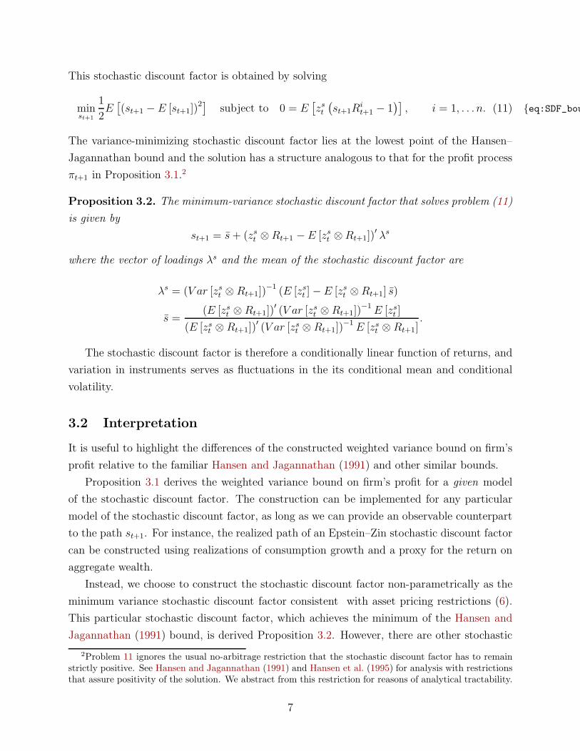
Figure 1: Extracted path of quarterly realizations of the minimum variance stochastic dis-count factor. NBER recessions shaded. The vector of returns used in the constructionincludes the S&P500 market return, 3M T-bill rate and returns on book-to-market andsize-sorted portfolios from Kenneth French’s website. The vector of instruments zst includesmarket tightness, vacancy filling rate, price-dividend ratio, output growth and the risk-freerate.

and construct the path for st+1. This path is depicted in Figure 1.

The path of the stochastic discount factor exhibits substantial countercyclical fluctuations

in conditional variance, with negligible movements in conditional mean. The stochastic

process for the stochastic discount factor needs to jointly rationalize countercyclical risk

premia and the relatively stable real risk-free rate. The countercyclical conditional variance

is consistent with structural models of the stochastic discount factor that involve stochastic

volatility in the consumption process at the business cycle frequency, or models with a

countercyclical price of risk, and additional restrictions are needed at this point to distinguish

between these interpretations.

5.1 Weighted variance bound

Instead, we use this constructed path of the stochastic discount factor as an input into the

construction of the variance bound for the firm’s profit process. We can now implement the

problem (7) using observable data for vacancy filling rates, separation rates and the path

of the stochastic discount factor. For alternative values of α ∈ (0, 1), we obtain a locus of

points in the space of the average conditional variance E [V art [πt+1]] and variance of the

conditional expectation V ar [Et [πt+1]] that form a bound above which all profit processes

satisfying restrictions (5) must lie.

Figure 2 depicts these bounds for several alternative stochastic discount factors. In the

10

0 0.5 1 1.5 20

0.25

0.5

Shimer (2010) Nash

Shimer (2010) rigid wage

Hall, Milgrom (2008)

Hall (2017)

NIPA profits

Compustat dividends

(E [V art [πt+1]])1/2

(Var[E

t[π

t+1]])1

/2

constant SDF

Rm, Rf , unconditional

Rm, Rf , conditioning

Rm, Rf , RBM , RME , conditioning

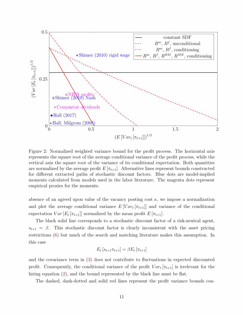
Figure 2: Normalized weighted variance bound for the profit process. The horizontal axisrepresents the square root of the average conditional variance of the profit process, while thevertical axis the square root of the variance of its conditional expectation. Both quantitiesare normalized by the average profit E [πt+1]. Alternative lines represent bounds constructedfor different extracted paths of stochastic discount factors. Blue dots are model-impliedmoments calculated from models used in the labor literature. The magenta dots representempirical proxies for the moments.

absence of an agreed upon value of the vacancy posting cost κ, we impose a normalization

and plot the average conditional variance E [V art [πt+1]] and variance of the conditional

expectation V ar [Et [πt+1]] normalized by the mean profit E [πt+1].

The black solid line corresponds to a stochastic discount factor of a risk-neutral agent,

st+1 = β. This stochastic discount factor is clearly inconsistent with the asset pricing

restrictions (6) but much of the search and matching literature makes this assumption. In

this case

Et [st+1πt+1] = βEt [πt+1]

and the covariance term in (3) does not contribute to fluctuations in expected discounted

profit. Consequently, the conditional variance of the profit V art [πt+1] is irrelevant for the

hiring equation (2), and the bound represented by the black line must be flat.

The dashed, dash-dotted and solid red lines represent the profit variance bounds con-

11

structed using alternative stochastic discount factors extracted by solving problem (11) for

different sets of returns that must be priced and different assumptions on conditioning. The

bounds our downward sloping, implying that the bound can be satisfied using a profit process

with high conditional volatility, or a high volatility of the conditional mean (i.e., a process

that is highly predictable), or a combination of both, as we move along the bound.

The bounds are showing that as we include additional returns that the stochastic discount

factor must price, and include relevant conditioning representing fluctuations in conditional

expected returns over the business cycle, the stochastic discount factor captures more of

the relevant macroeconomic risks, and the bound can be satisfied with a lower conditional

volatility of the profit flow E [V art [πt+1]]. This is representing by the bounds becoming

steeper in Figure 2.

Interestingly, the intersects of the bounds with the vertical axis also lie higher when

the stochastic discount factor prices relevant asset returns. The reason has to do with the

procyclicality of the real interest rate. Consider the case when we want to satisfy the bound

with a profit flow that is perfectly predictable and hence V art [πt+1] = 0. Such a profit low

will lie on the vertical axis in Figure 2. In that case

Et [st+1πt+1] = Et [st+1]Et [πt+1] .

When Et [st+1] = β, as in the case of the black line, the conditional expectation of the profit

flow Et [πt+1] must be sufficiently procyclical to rationalize the evolution of hiring over the

business cycle. At the same time, when the stochastic discount is supposed to correctly price

the risk-free rate, which is mildly procyclical, Et [st+1] must be mildly countercyclical. This

implies that Et [πt+1] must be even more procyclical than in the case when Et [st+1] = β,

and the bound tightens.

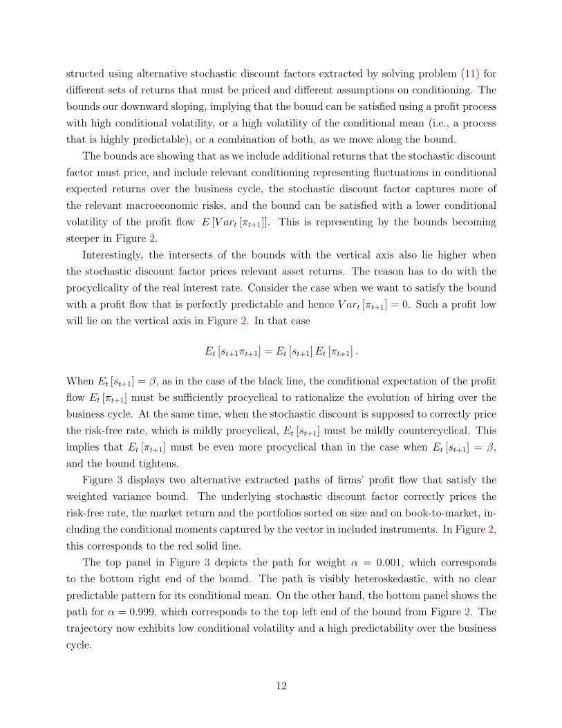
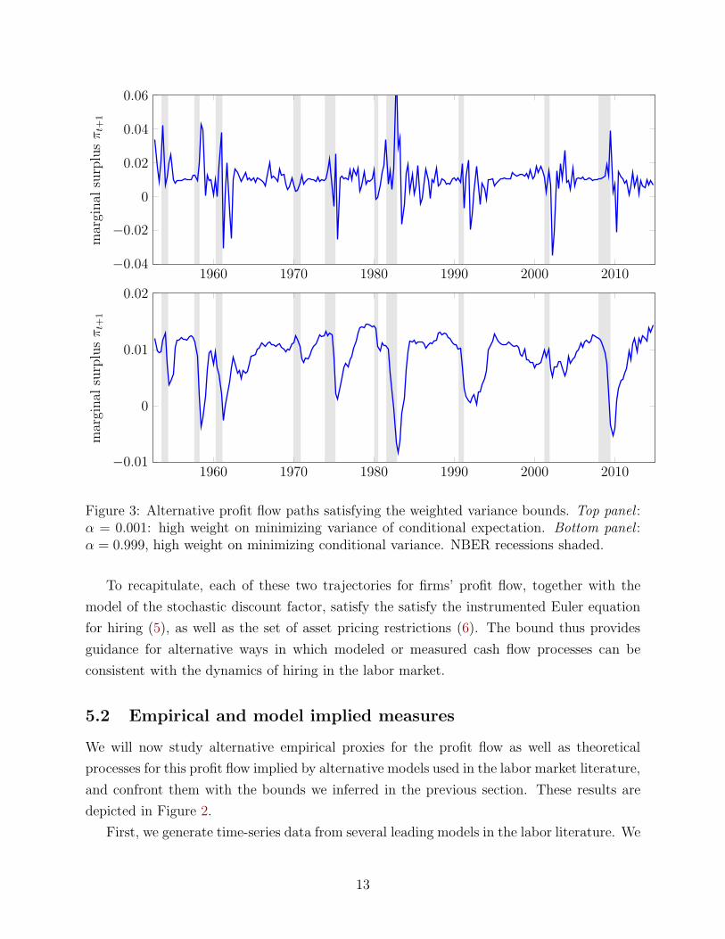
Figure 3 displays two alternative extracted paths of firms’ profit flow that satisfy the

weighted variance bound. The underlying stochastic discount factor correctly prices the

risk-free rate, the market return and the portfolios sorted on size and on book-to-market, in-

cluding the conditional moments captured by the vector in included instruments. In Figure 2,

this corresponds to the red solid line.

The top panel in Figure 3 depicts the path for weight α = 0.001, which corresponds

to the bottom right end of the bound. The path is visibly heteroskedastic, with no clear

predictable pattern for its conditional mean. On the other hand, the bottom panel shows the

path for α = 0.999, which corresponds to the top left end of the bound from Figure 2. The

trajectory now exhibits low conditional volatility and a high predictability over the business

cycle.

12

1960 1970 1980 1990 2000 2010−0.04

−0.02

0

0.02

0.04

0.06marginal

surplusπt+

1

1960 1970 1980 1990 2000 2010−0.01

0

0.01

0.02

marginal

surplusπt+

1

Figure 3: Alternative profit flow paths satisfying the weighted variance bounds. Top panel :α = 0.001: high weight on minimizing variance of conditional expectation. Bottom panel :α = 0.999, high weight on minimizing conditional variance. NBER recessions shaded.

To recapitulate, each of these two trajectories for firms’ profit flow, together with the

model of the stochastic discount factor, satisfy the satisfy the instrumented Euler equation

for hiring (5), as well as the set of asset pricing restrictions (6). The bound thus provides

guidance for alternative ways in which modeled or measured cash flow processes can be

consistent with the dynamics of hiring in the labor market.

5.2 Empirical and model implied measures

We will now study alternative empirical proxies for the profit flow as well as theoretical

processes for this profit flow implied by alternative models used in the labor market literature,

and confront them with the bounds we inferred in the previous section. These results are

depicted in Figure 2.

First, we generate time-series data from several leading models in the labor literature. We

13

start with the model in Shimer (2010), Section 3.3, which extends the standard search model

by including capital and considering shocks to productivity as well as to the separation rate.

Importantly, the wage is determined by Nash bargaining so this model does not generate

enough business cycle movements in employment. In that respect, it is similar to Shimer

(2005). We further consider the model in Section 4.3 in Shimer (2010) which replaces the

Nash bargaining mechanism with a backward-looking wage setting. The actual wage is a

weighted average of last period’s wage, and the current target wage, where the target wage

is the one which solves the Nash bargaining problem. This is an ad-hoc wage setting rule

but the goal is to study whether this helps to amplify employment fluctuations.

Two other models we examine are Hall and Milgrom (2008) and Hall (2017) which both

aim at generating large fluctuations in employment. Hall and Milgrom (2008) introduce

wage rigidity into an otherwise standard search model, and Hall (2017) adds movements in

the stochastic discount factor on top of the wage rigidity.

For each of these models, we generate the time-series of profit flow πt and all state

variables. We then construct E[V art[πt+1]] and V ar[Et[πt+1]] by forecasting πt+1 using the

time-t state variables implied by the model dynamics. We normalize both objects by the

mean value of the profit flow, E[πt+1].

Figure 2 shows the results, each blue dot representing one these models. Three out of four

analyzed models lie below all displayed bounds. First, these three models lie below the black

line representing the constant SDF case. Indeed, Shimer (2010) uses a stochastic discount

factor that is essentially constant and shows that the model with Nash bargaining does not

generate enough employment fluctuations. Figure 2 not only confirms this finding but also

shows that if we kept fixed the stochastic process for profit flow obtained from the Shimer

(2010) model with Nash bargaining, and coupled it with alternative stochastic discount

factors that we constructed previously, the model would still not be able to rationalize the

Euler equation for hiring (2), and therefore would continue to understate the magnitude of

employment fluctuations.

The same conclusion holds for the Hall and Milgrom (2008) model. On the other hand, the

version of Shimer (2010) with backward-looking wage setting rules lies above the constructed

bounds, meaning that the modeled profit flow process combines enough volatility through

E [V art [πt+1]] and V ar [Et [πt+1]] to satisfy the hiring Euler equation, and therefore has the

potential to match the magnitude of employment fluctuations observed in the data.

Interestingly, the model from Hall (2017) lies below all displayed bounds, which leads us

to conclude that the model enough movements in the profit flow to satisfy (2). This is not the

conclusion that the author reaches in that paper, though. The reason for this discrepancy

is that we require the stochastic discount factor to be consistent with the cyclical properties

14

of the risk-free rate. Hall (2017) does not impose such restriction and the fluctuations in

Et [st+1πt+1] are rationalized by highly procyclical fluctuations in Et [st+1] that generate a

counterfactually large countercyclical volatility in the real risk-free rate. We will return to

this issue in Section 5.4 where we provide an alternative interpretation of the profit flow

process πt+1 that potentially reconciles these differences.

Next we construct a pair of empirical proxies for the profit flow. First, we construct

real profits per worker using after-tax corporate profits from NIPA (variable CP in FRED),

divided by the GDP deflator (GDPDEF) and employment (CE16OV). We detrend the time

series by real potential GDP per capita (GDPPPOT/CNP16OV).

We also measure real per capita profits in Compustat. We use operating income be-

fore depreciation (OIBDPQ), deflated by the GDP deflator and divided by employment as

measured in Compustat. Employment in Compustat is available only at annual frequency,

and we linearly interpolate the data to obtain a quarterly data series. We again detrend by

dividing the time series by real potential GDP per capita.

For both proxies of the profits, we compute E[V art[πt+1]] and V ar[Et[πt+1]] using a

projection on the vector of instruments used in equations (5) and (6). We again normalize

both objects by the mean value of the profit flow, E[πt+1]. Magenta dots in Figure 2 represent

these data.

It is important to stress the discrepancy between these measures of profit per worker

and the theoretical object we are interested in. The theoretical model predicts that πt+1

corresponds to the profit flow from the marginal worker. Constructed empirical proxies,

however, represents average profits per worker. Hence a failure of an empirical proxy to

meet the bound can potentially be attributable to the discrepancy between average and

marginal profits from a worker. In absence of empirical measures of marginal profits, one

potential avenue is to use the distance between the data points and the bound as a constraint

on the wedge implied by a theoretical model that distinguishes between average and marginal

worker profit.

5.3 Predicted unemployment path

We further examine whether fluctuations in the value of the job can explain fluctuations

in the unemployment rate. To do so, we construct a time path for the value of a worker

J (Xt) and feed the path into the model in order to generate a predicted time path for the

unemployment rate.

For this exercise, we need to choose the functional form for the matching function. We

assume a constant returns to scale matching function q (θ) = Bθ−η. We choose the elasticity

15

1960 1970 1980 1990 2000 20100

0.5

1Std

t(s t

+1)

Figure 4: SDF volatility NBER recessions shaded.

η = 0.72 following Shimer (2005), and normalize B to match the mean of the unemployment

rate in the simulated path with the mean in the data.

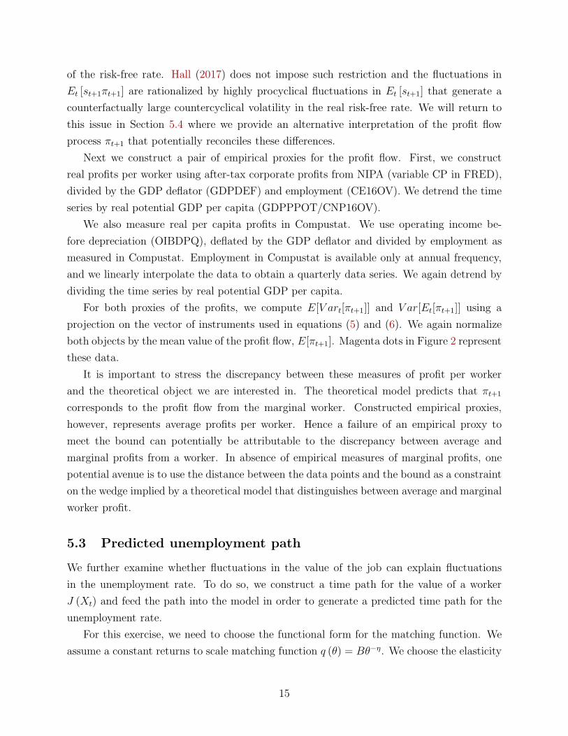
We now proceed as follows. First, we estimate the model (12) using the observable time

series for st+1, πt+1 and δt+1. Figure 4 plots the conditional volatility of the stochastic

discount factor(bvols Xt

)|bws | and confirms the substantial heteroskedasticity implied by the

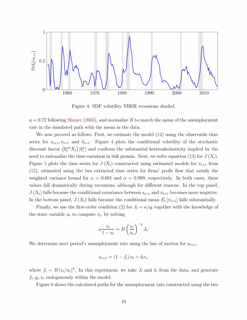
need to rationalize the time-variation in risk premia. Next, we solve equation (13) for J (Xt).

Figure 5 plots the time series for J (Xt) constructed using estimated models for πt+1 from

(12), estimated using the two extracted time series for firms’ profit flow that satisfy the

weighted variance bound for α = 0.001 and α = 0.999, respectively. In both cases, these

values fall dramatically during recessions, although for different reasons. In the top panel,

J (Xt) falls because the conditional covariance between st+1 and πt+1 becomes more negative.

In the bottom panel, J (Xt) falls because the conditional mean Et [πt+1] falls substantially.

Finally, we use the first-order condition (2) for Jt = κ/qt together with the knowledge of

the state variable ut to compute vt, by solving

κvt

1− ut= B

(vtut

)−η

Jt.

We determine next period’s unemployment rate using the law of motion for ut+1,

ut+1 = (1− ft) ut + δtet,

where ft = B (vt/ut)η. In this experiment, we take Jt and δt from the data, and generate

ft, qt, vt endogenously within the model.

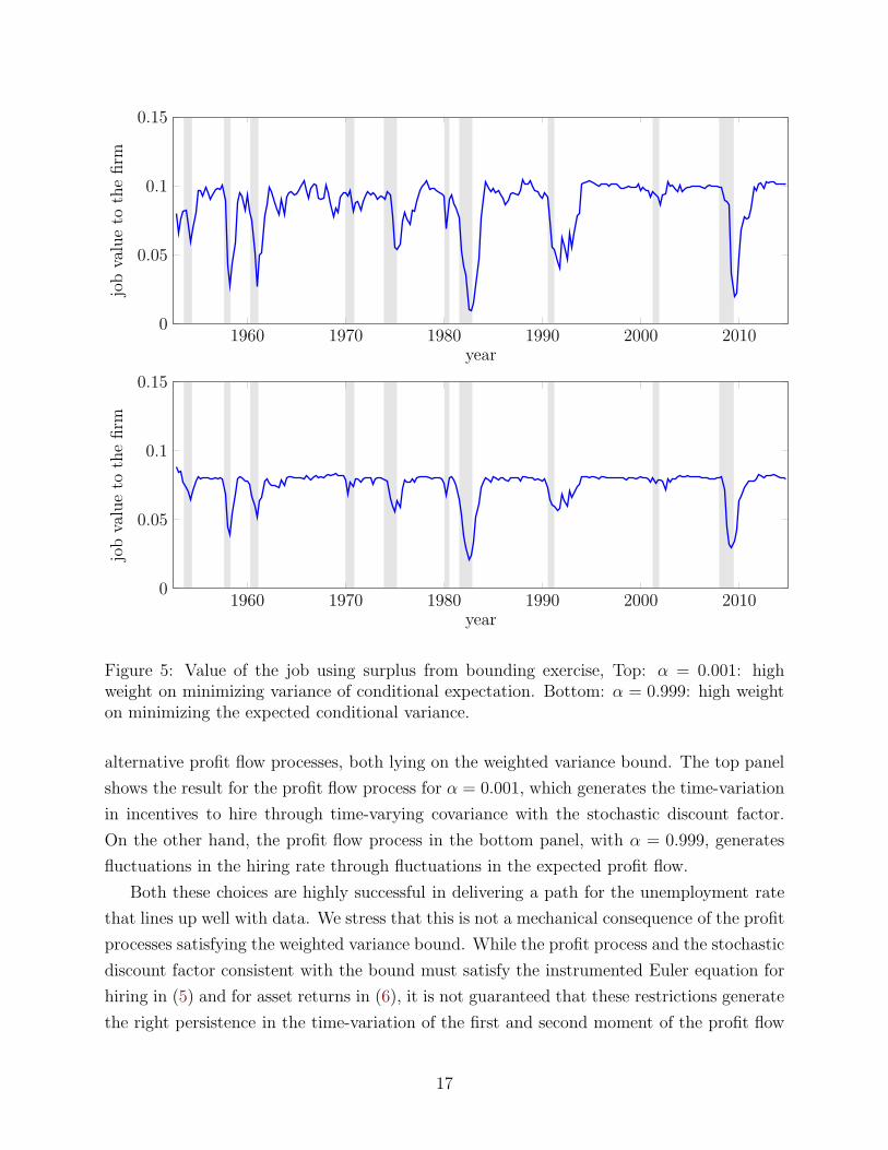
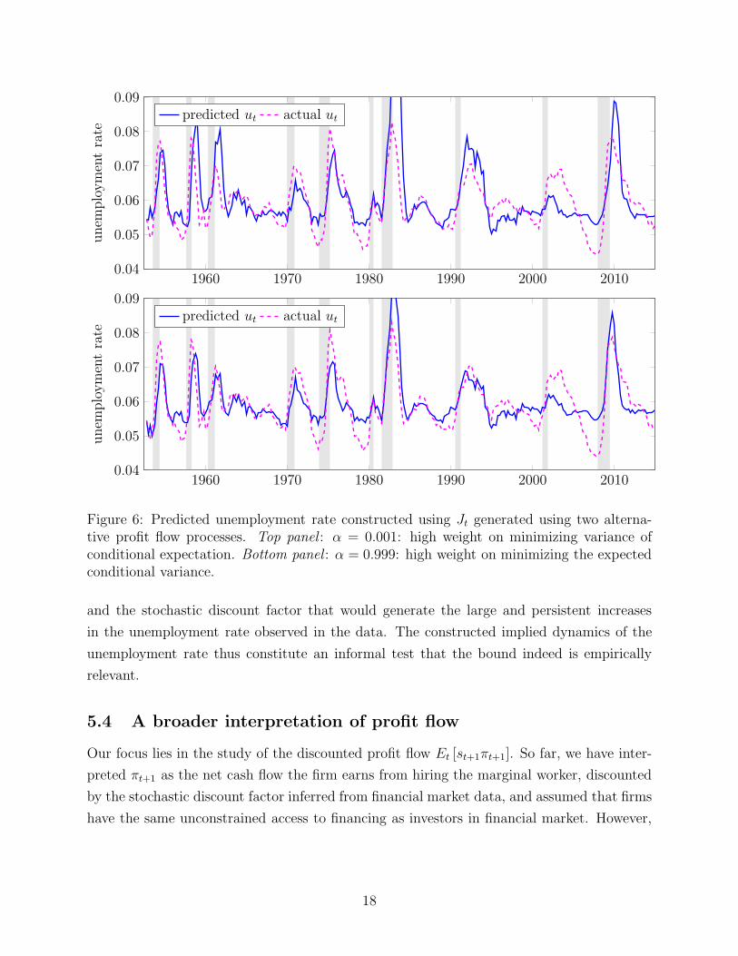
Figure 6 shows the calculated paths for the unemployment rate constructed using the two

16

1960 1970 1980 1990 2000 20100

0.05

0.1

0.15

year

jobvalueto

thefirm

1960 1970 1980 1990 2000 20100

0.05

0.1

0.15

year

jobvalueto

thefirm

Figure 5: Value of the job using surplus from bounding exercise, Top: α = 0.001: highweight on minimizing variance of conditional expectation. Bottom: α = 0.999: high weighton minimizing the expected conditional variance.

alternative profit flow processes, both lying on the weighted variance bound. The top panel

shows the result for the profit flow process for α = 0.001, which generates the time-variation

in incentives to hire through time-varying covariance with the stochastic discount factor.

On the other hand, the profit flow process in the bottom panel, with α = 0.999, generates

fluctuations in the hiring rate through fluctuations in the expected profit flow.

Both these choices are highly successful in delivering a path for the unemployment rate

that lines up well with data. We stress that this is not a mechanical consequence of the profit

processes satisfying the weighted variance bound. While the profit process and the stochastic

discount factor consistent with the bound must satisfy the instrumented Euler equation for

hiring in (5) and for asset returns in (6), it is not guaranteed that these restrictions generate

the right persistence in the time-variation of the first and second moment of the profit flow

17

1960 1970 1980 1990 2000 20100.04

0.05

0.06

0.07

0.08

0.09unem

ploymentrate

predicted ut actual ut

1960 1970 1980 1990 2000 20100.04

0.05

0.06

0.07

0.08

0.09

unem

ploymentrate

predicted ut actual ut

Figure 6: Predicted unemployment rate constructed using Jt generated using two alterna-tive profit flow processes. Top panel : α = 0.001: high weight on minimizing variance ofconditional expectation. Bottom panel : α = 0.999: high weight on minimizing the expectedconditional variance.

and the stochastic discount factor that would generate the large and persistent increases

in the unemployment rate observed in the data. The constructed implied dynamics of the

unemployment rate thus constitute an informal test that the bound indeed is empirically

relevant.

5.4 A broader interpretation of profit flow

Our focus lies in the study of the discounted profit flow Et [st+1πt+1]. So far, we have inter-

preted πt+1 as the net cash flow the firm earns from hiring the marginal worker, discounted

by the stochastic discount factor inferred from financial market data, and assumed that firms

have the same unconstrained access to financing as investors in financial market. However,

18

if firms face financial constraints, then the corresponding discounted profit flow is given by

Et [st+1λt+1πt+1].= Et [st+1πt+1]

where πt+1 is the profit flow adjusted by the shadow prices of the borrowing constraints in

individual future states relative to today, λt+1. These shadow prices emerge, for instance, in

situations when firms need to borrow to finance the cost of hiring or to pre-pay wages. In

such situations, an empirical proxy for profits constructed using NIPA or Compustat data

would provide a biased measure of πt+1, and λt+1 could explain, at least to some extent,

the distance between the magenta points in Figure 2 and the weighted variance bounds.

To answer this question, one needs to construct an empirical or theoretical measure of the

fluctuations in these shadow prices λt+1.

This interpretation also provides a possible reconciliation between our bound and the

results in the Hall (2017) model. If we write the discounted profit flow as Et [st+1πt+1]

where st+1 = st+1λt+1, then st+1 would not be the stochastic discount factor pricing assets in

unconstrained markets but rather a constraint-adjusted stochastic discount factor that takes

into account the role of pricing impact of constrained borrowing. We leave the exploration

of this topic for future work.

6 Structural model

In the previous sections, we non-parametrically inferred the dynamics of a stochastic discount

factor and a profit process that satisfied a lower bound on their second moments that made

them consistent with restrictions on pricing of return and on hiring choices. We now impose

more structure on the stochastic discount factor, and use an empirical counterpart of the

profit flow series in order to investigate whether these restrictions are still consistent with

the labor market dynamics.

The model economy is populated by a representative household and heterogeneous firms

operating in frictional labor markets that are subject to financial constraints. Time is dis-

crete, t = 0, 1, 2, . . ., and we assume that aggregate uncertainty is driven by a state vector

Xt that follows the vector-autoregression

Xt+1 = ψxXt + ψwWt+1 (14) {eq:VAR}

where ψx and ψw are conforming matrices and Wt+1 ∼ N (0, I) is an iid multivariate normal

vector of innovations.

19

6.1 Household preferences

The representative household is endowed with Epstein and Zin (1989) preferences with uni-

tary elasticity of substitution:3

Ut = (1− β) logCt −β

θtlogEt [exp (−θtUt+1)] (15) {eq:EZ_preferences

where β is the time-preference parameter and γt.= θt + 1 is the time-varying risk-aversion

parameter.4 The preference structure (15) implies the one-period stochastic discount factor

St+1

St= β

(Ct+1

Ct

)−1

exp (−θtUt+1)

Et [exp (−θtUt+1)].

The time-variation in the risk-aversion parameter scales the volatility of the last term in the

stochastic discount factor. This introduces time-varying prices of risk into our model, and

hence fluctuations in discounting of risky cash flows. The dynamics of θt will be consistent

with the dynamics of equilibrium returns, and we will infer it from fluctuations in risk premia.

In order to operationalize this model, we assume that the growth rate in aggregate

consumption follows

∆ct+1.= logCt+1 − logCt = ι′cXt. (16) {eq:consumption_growth

For instance, ιc can be an indicator vector that selects ∆ct from the VAR. In Section 6.2,

we show that under additional assumptions on the distribution of conditional returns, the

dynamics of the risk aversion parameter θt and the continuation value Ut satisfy

θt = ι′θXt (17) {eq:theta_X

and

Ut = logCt + u′Xt (18) {eq:EZ_preferences_guess

where ιθ and u are vectors determined in equilibrium. The calculations are detailed in

Appendix A.

3A generalization to non-unitary elasticity of substitution can be obtained by a linear expansion aroundthe unitary case.

4The time-variation in the risk-aversion parameter offers alternative interpretations. Campbell andCochrane (1999) is the seminal contribution in the context of an external habit model. Dew-Becker (2014)embeds this framework into the Epstein–Zin preference structure. See also Greenwald et al. (2014), Kozak(2015) and Kozak and Santosh (2016). Bhandari et al. (2016) interpret this time-variation in the context ofrobust preferences, see also Hansen and Sargent (2015).

20

6.2 Asset pricing implications

The representative household invests its wealth into a portfolio of assets indexed by i, with

gross returns Rit+1. Optimality conditions imply that asset returns have to satisfy the Euler

equations

1 = Et

[St+1

St

Rit+1

].

Under the assumption of log-normally distributed returns, we show in the appendix that the

expected excess return (risk premium) on asset i can be written as

Et

[rit+1

]+

1

2V art

[rit+1

]− rft = (θt + 1)Covt

(rwt+1, r

it+1

)+ θtCovt

(u′Xt+1, r

it+1

)(19) {eq:risk_premium

where rit+1 = logRit+1, r

ft is the risk-free rate between periods t and t + 1, and rwt+1 is the

return on household’s wealth. Further assuming that we can identify the return on wealth

with the return on the market portfolio, and the excess returns can be inferred from the

VAR,

rxwt+1.= rwt+1 − rft = ι′rxwXt+1,

we can use the pricing equation (19) for rit+1 = rwt+1 to infer the path of θt:

θt =i′rxwψxXt −

12V art

[rwt+1

]

V art[rwt+1

]+ u′ψwψ′

wirxw=i′rxwψxXt −

12i′rxwψwψ

′

wirxw

(irxw + u)′ ψwψ′

wirxw

.= i′θXt. (20) {eq:itheta}

Equation (20) determines the loadings of the time-varying price of risk inferred from the

equilibrium dynamics of returns in the VAR given by (14). This equation, together with

equation (25) in the appendix, can be jointly solved for the vectors u and ιθ.

6.3 Firms and labor market

We consider a model of a firm that faces financial constraints. The firm enters period t

with a stock of capital kt, labor force lt, and debt bt. Aggregate and firm-specific shocks are

realized and production takes place. The firm pays out wages and interest on its borrowing.

Some workers separate from the firm for exogenous reasons, and capital depreciates. The

firm then posts vacancies ξt to hire new workers, invests into capital, pays out dividends and

decides on new borrowing.

The financial position of the firm before the capital investment is captured by its net

worth

nt = yt − wtlt − κ (ξt) +(1− δk

)Qtkt − Rb

tbt

21

where yt is the produced output, wtlt total wage bill, κ (ξt) total vacancy cost,(1− δk

)Qtkt

market value of undepreciated capital, and Rbtbt the market value of repayed debt. New

capital kt+1 is financed by net worth after the divided payout dt, and by issuance of new

bonds bt+1:

Qtkt+1 = nt − dt + bt+1. (21) {eq:balance_sheet_constra

The laws of motion for firm’s labor force and capital stock are given by

lt+1 = qtξt +(1− δlt

)lt

kt+1 = it +(1− δk

)kt.

Here, qt is the probability of filling a vacancy posted by the firm, and δlt the possibly time-

varying worker separation rate. In the conventional Diamond–Mortensen–Pissarides search-

and-matching framework, this vacancy filling probability is tied to aggregate labor market

conditions.

The firm maximizes the present discounted value of dividends, implying that the value

function is given by

Vt (kt, lt, bt) = maxit,ξt,bt+1,dt

dt + Et

[St+1

StVt+1 (kt+1, lt+1, bt+1)

]

where the expectations operator integrates over firm-specific and aggregate sources of un-

certainty. We assume that firms are owned by a representative household, and hence they

discount cash flows using the households’ stochastic discount S. The stochastic discount

factor is specified in Section 6.1.

Firms are subject to constraints that limit their ability to acquire outside financing to

finance their labor costs and acquisition of new capital. The literature provides microfounda-

tions for a whole variety of functional forms for the financial constraint that can be broadly

written in the form

F (kt+1, lt+1, bt+1, kt, lt, bt) ≥ 0.

As an illustration for the derivation of the optimality conditions, we specialize the constraint

to the form

nt − φkQtkt+1 ≥ 0. (22) {eq:financial_constraint_

This is a leverage constraint, stating that the ratio of net worth to the market value of

capital has to be at least φk. In order to limit the ability of the firm to outsave the financial

22

constraint, we enforce an exogenous dividend policy

dt = dnt.

Imposing Lagrange multipliers µt and λt on the balance sheet constraint (21) and financial

constraint (22), respectively, we obtain the Euler equation for the hiring decision5

κ′ (ξt)

qt= Et

[St+1

St

d+(1− d

)µt+1 + λt+1

d+(1− d

)µt + λt

(∂yt+1

∂lt+1

− wt+1 +(1− δlt+1

) κ′ (ξt+1)

qt+1

)]. (23) {eq:EE_hiring

The equation equalizes the marginal cost of hiring a worker, κ′ (ξt) /qt, with the expected

discounted benefits to the firm next period from hiring this worker. The benefits consist

of the period surplus accrued by the firm, given by the marginal product of the worker

∂yt+1/∂lt+1 net of wage wt+1, plus the saved cost from not having to hire the worker next

period, in case the worker does not separate. The second term in brackets reflects the

impact of the financial constraint. In case of an unconstrained firm with optimally chosen

dividends, λt = 0 and µt = 1. Otherwise financial constraints impact firm’s hiring decisions.

When financial constraints are tighter relative to next period, the second term in brackets

is smaller than one, and effectively operates as an additional source of discounting of next

period benefits.

6.4 Valuation of firms’ cash flows

The Euler equation (23) can be solved forward for the value of the job as the present dis-

counted value of future cash flows from the match acquired by the firm

κ′ (ξt)

qt=

∞∑

j=1

Et

[St+j

St

Ft+j

Ft

(j∏

i=1

(1− δlt+i

))Gt+j

].= Jt (24) {eq:J_PDV}

where

Gt+j =∂yt+j

∂lt+j− wt+j

Ft+j

Ft

=d+

(1− d

)µt+1 + λt+1

d+(1− d

)µt + λt

.

5The remaining derivations are in Appendix A.

23

Similarly, we can denote

Ht+j

Ht=

j∏

i=1

(1− δlt+i

).

The current value of a job for the firm, Jt, is thus represented by its future cash flows, Gt+j ,

discounted by the household’s stochastic discount factor, cumulative probability of future

job separation, and the contribution from future financial constraints. Notice that tighter

financial constraints in the future increase the value of the job, since an existing job reduces

the need for costly vacancy posting in states when financial constraints are tight.

Since observed separation rates δlt are high, the value of a job consists of cash flows that

have on average shorter maturity than, for instance, cash flows received by shareholders. To

the extent that shorter maturity cash flows appear to earn higher risk compensations (see

van Binsbergen et al. (2013) and the subsequent quickly growing literature), we can plausibly

expect the same for the cash flows constituting the value of the job for the firm.

In what follows, we will study the value of the job Jt constructed from estimated dis-

counted cash flows. The empirical challenge in the search-and-matching literature is to make

the value of the job sufficiently volatile so as to make it consistent with large cyclical fluctua-

tions in vacancy posting rates ξt and job filling probabilities qt, represented by the left-hand

side of (24). We will study the separate contributions of discount rate fluctuations, captured

by movements in θt, tightness in financial constraints, and separation rates on Jt.

7 Data and empirical implementation

In addition to the variables described in Section 4, we use additional macroeconomic variables

to capture the dynamics of the state vector Xt. The names of these variables as they appear

in FRED are in parenthesis.

The real per capita consumption growth is constructed from expenditures on nondurable

goods (PCESV) and services (PCND), adjusted for inflation (CPIAUCNS) and population

growth (CNP16OV). The real income growth corresponds to real personal disposable income

(DPIC96), adjusted for population growth.

Firm’s cash flow from hiring a worker equals marginal product of labor minus the wage.

We measure the marginal product of labor as (1− α)Yt/Lt where Yt is real GDP (GDPC1),

Lt is employment (CE16OV), and we choose α = 1/3. To construct a quarterly measure

of wages since 1952, we combine two variables: the index of real compensation per hour in

non-farm business sector (COMPRNFB) and the average weekly wage for a given quarter

(avg wkly wage) from the BLS website. While the time series for the former variable starts

in 1947, it is only constructed as an index. On the other hand, the latter represents the

24

wage level but only starts in 1975. We use the average weekly wage to convert the index to

dollars.

8 Results

We start by estimating the VAR (14). Our choice of variables follows Bansal et al. (2014),

extended by a measure of the aggregate separation rate. The state vector is given by

Xt =(1,∆ct, rx

mt ,∆yt, pdt, r

ft ,∆ht

)

where ∆ct is real consumption growth per capita, rxmt market (S&P 500) excess return, ∆yt is

the real disposable income growth per capita, pdt the price-dividend ratio, ∆gt growth rate

of firm surplus, rft real risk-free rate, and ∆ht.= log

(1− δlt

)the logarithm of one-period

match survival rate.

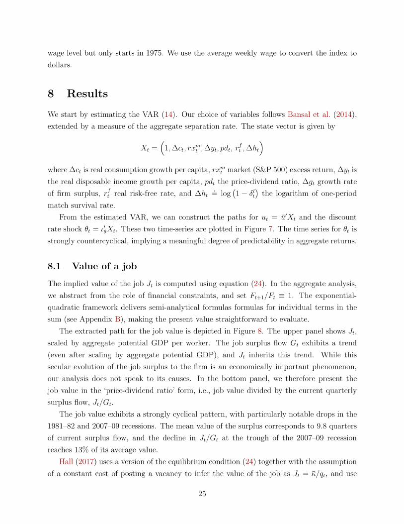
From the estimated VAR, we can construct the paths for ut = u′Xt and the discount

rate shock θt = ι′θXt. These two time-series are plotted in Figure 7. The time series for θt is

strongly countercyclical, implying a meaningful degree of predictability in aggregate returns.

8.1 Value of a job

The implied value of the job Jt is computed using equation (24). In the aggregate analysis,

we abstract from the role of financial constraints, and set Ft+1/Ft ≡ 1. The exponential-

quadratic framework delivers semi-analytical formulas formulas for individual terms in the

sum (see Appendix B), making the present value straightforward to evaluate.

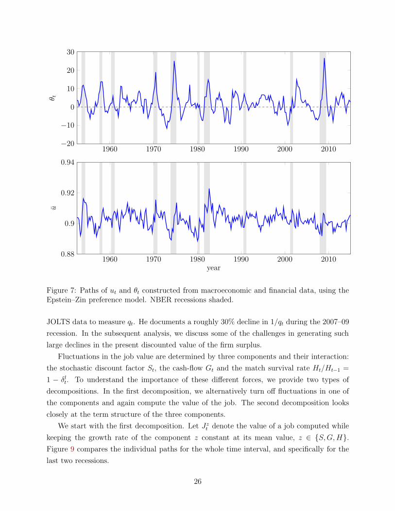
The extracted path for the job value is depicted in Figure 8. The upper panel shows Jt,

scaled by aggregate potential GDP per worker. The job surplus flow Gt exhibits a trend

(even after scaling by aggregate potential GDP), and Jt inherits this trend. While this

secular evolution of the job surplus to the firm is an economically important phenomenon,

our analysis does not speak to its causes. In the bottom panel, we therefore present the

job value in the ‘price-dividend ratio’ form, i.e., job value divided by the current quarterly

surplus flow, Jt/Gt.

The job value exhibits a strongly cyclical pattern, with particularly notable drops in the

1981–82 and 2007–09 recessions. The mean value of the surplus corresponds to 9.8 quarters

of current surplus flow, and the decline in Jt/Gt at the trough of the 2007–09 recession

reaches 13% of its average value.

Hall (2017) uses a version of the equilibrium condition (24) together with the assumption

of a constant cost of posting a vacancy to infer the value of the job as Jt = κ/qt, and use

25

1960 1970 1980 1990 2000 2010−20

−10

0

10

20

30θ t

1960 1970 1980 1990 2000 20100.88

0.9

0.92

0.94

year

u

Figure 7: Paths of ut and θt constructed from macroeconomic and financial data, using theEpstein–Zin preference model. NBER recessions shaded.

JOLTS data to measure qt. He documents a roughly 30% decline in 1/qt during the 2007–09

recession. In the subsequent analysis, we discuss some of the challenges in generating such

large declines in the present discounted value of the firm surplus.

Fluctuations in the job value are determined by three components and their interaction:

the stochastic discount factor St, the cash-flow Gt and the match survival rate Ht/Ht−1 =

1 − δlt. To understand the importance of these different forces, we provide two types of

decompositions. In the first decomposition, we alternatively turn off fluctuations in one of

the components and again compute the value of the job. The second decomposition looks

closely at the term structure of the three components.

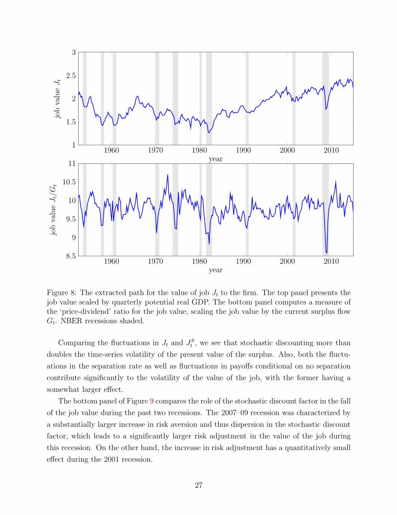
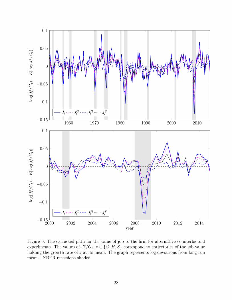
We start with the first decomposition. Let Jzt denote the value of a job computed while

keeping the growth rate of the component z constant at its mean value, z ∈ {S,G,H}.

Figure 9 compares the individual paths for the whole time interval, and specifically for the

last two recessions.

26

1960 1970 1980 1990 2000 20101

1.5

2

2.5

3

year

jobvalueJt

1960 1970 1980 1990 2000 20108.5

9

9.5

10

10.5

11

year

jobvalueJt/G

t

Figure 8: The extracted path for the value of job Jt to the firm. The top panel presents thejob value scaled by quarterly potential real GDP. The bottom panel computes a measure ofthe ‘price-dividend’ ratio for the job value, scaling the job value by the current surplus flowGt. NBER recessions shaded.

Comparing the fluctuations in Jt and JSt , we see that stochastic discounting more than

doubles the time-series volatility of the present value of the surplus. Also, both the fluctu-

ations in the separation rate as well as fluctuations in payoffs conditional on no separation

contribute significantly to the volatility of the value of the job, with the former having a

somewhat larger effect.

The bottom panel of Figure 9 compares the role of the stochastic discount factor in the fall

of the job value during the past two recessions. The 2007–09 recession was characterized by

a substantially larger increase in risk aversion and thus dispersion in the stochastic discount

factor, which leads to a significantly larger risk adjustment in the value of the job during

this recession. On the other hand, the increase in risk adjustment has a quantitatively small

effect during the 2001 recession.

27

1960 1970 1980 1990 2000 2010−0.15

−0.1

−0.05

0

0.05

0.1log(J

z t/G

t)−E[log(J

z t/G

t)]

Jt JGt JH

t JSt

2000 2002 2004 2006 2008 2010 2012 2014−0.15

−0.1

−0.05

0

0.05

0.1

year

log(J

z t/G

t)−E[log(J

z t/G

t)]

Jt JGt JH

t JSt

Figure 9: The extracted path for the value of job to the firm for alternative counterfactualexperiments. The values of Jz

t /Gt, z ∈ {G,H, S} correspond to trajectories of the job valueholding the growth rate of z at its mean. The graph represents log deviations from long-runmeans. NBER recessions shaded.

28

1960 1970 1980 1990 2000 2010−0.02

0

0.02

0.04

0.06excess

yields(%

)j = 1 j = 8 j = 20

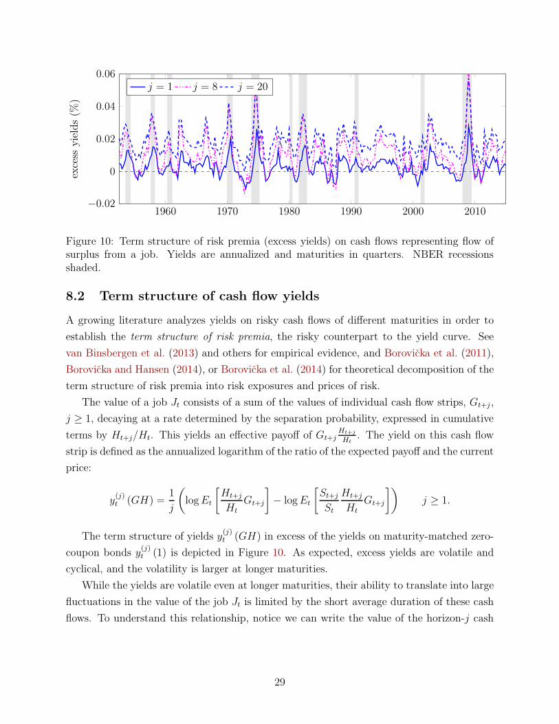
Figure 10: Term structure of risk premia (excess yields) on cash flows representing flow ofsurplus from a job. Yields are annualized and maturities in quarters. NBER recessionsshaded.

8.2 Term structure of cash flow yields

A growing literature analyzes yields on risky cash flows of different maturities in order to

establish the term structure of risk premia, the risky counterpart to the yield curve. See

van Binsbergen et al. (2013) and others for empirical evidence, and Borovicka et al. (2011),

Borovicka and Hansen (2014), or Borovicka et al. (2014) for theoretical decomposition of the

term structure of risk premia into risk exposures and prices of risk.

The value of a job Jt consists of a sum of the values of individual cash flow strips, Gt+j ,

j ≥ 1, decaying at a rate determined by the separation probability, expressed in cumulative

terms by Ht+j/Ht. This yields an effective payoff of Gt+jHt+j

Ht. The yield on this cash flow

strip is defined as the annualized logarithm of the ratio of the expected payoff and the current

price:

y(j)t (GH) =

1

j

(logEt

[Ht+j

Ht

Gt+j

]− logEt

[St+j

St

Ht+j

Ht

Gt+j

])j ≥ 1.

The term structure of yields y(j)t (GH) in excess of the yields on maturity-matched zero-

coupon bonds y(j)t (1) is depicted in Figure 10. As expected, excess yields are volatile and

cyclical, and the volatility is larger at longer maturities.

While the yields are volatile even at longer maturities, their ability to translate into large

fluctuations in the value of the job Jt is limited by the short average duration of these cash

flows. To understand this relationship, notice we can write the value of the horizon-j cash

29

flow strip as

Et

[St+j

St

Ht+j

Ht

Gt+j

]= Et

[St+j

St

]

︸ ︷︷ ︸risk-free discounting

Et

[Ht+j

Ht

Gt+j

]

︸ ︷︷ ︸expected

cash flow

+ Covt

(St+j

St

,Ht+j

Ht

Gt+j

)

︸ ︷︷ ︸risk compensation

.

This formula decomposes the strip value into the contribution of risk-free discounting of ex-

pected cash flows (the first term on the right-hand side), and the risk-premium contribution,

represented by the covariance term.

When shocks to the stochastic discount factor and cash flow growth rates are persistent,

then their effects accumulate over time. Much of the search-and-matching literature focused

on modeling the time-variation in expected cash flows, either through time-variation in match

productivity, or alternative surplus sharing rules between the worker and the firm. Another

possibility of generating fluctuations in the value of the cash-flow is through changes in the

conditional risk-free rate, but given the smoothness of real risk-free rates in the data, this

does not appear to be a quantitatively important channel.

The discount rate shock θt in our framework is a persistent shock that affects the dis-

persion of the stochastic discount factor, and hence the risk compensation represented by

the covariance term above. Again, since the shock is persistent, its effects accumulate with

maturity, and we may also expect larger effects for cash flows with longer maturities.

Unfortunately, the impact of persistent shocks on Jt through fluctuations in the value

of long-horizon cash flows is dampened by the decay rate Ht+j/Ht. Since separations are

larger (of the order of 10% per quarter, implying an average maturity of the cash flows of

2.5 years), expected flow of surplus from long-maturity strips quickly becomes negligible as

maturity grows. This is in contrast to, for instance, price-dividend ratios since dividends

have a much higher average duration.

In this aggregate analysis, we abstract from the role of financial constraints, introduced

in the formula (24). Financial constraints Ft+1/Ft would be manifested as another term in

the above decomposition. We devote our attention to the role of financial constraints in our

cross-sectional analysis.

8.3 Predicted unemployment path

We now repeat the exercise conducted in Section 5.3 and construct the inferred path for

unemployment from the time series of the continuation values Jt, vacancy data, and the

imposed matching function. In order to deal with the non-stationarity of the continuation

30

1960 1970 1980 1990 2000 20100.04

0.05

0.06

0.07

0.08

0.09unem

ploymentrate

predicted ut actual ut

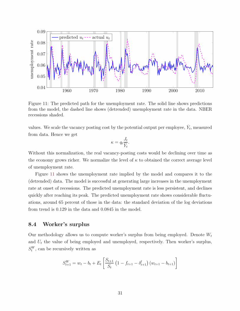
Figure 11: The predicted path for the unemployment rate. The solid line shows predictionsfrom the model, the dashed line shows (detrended) unemployment rate in the data. NBERrecessions shaded.

values. We scale the vacancy posting cost by the potential output per employee, Yt, measured

from data. Hence we get

κ = qtJtYt.

Without this normalization, the real vacancy-posting costs would be declining over time as

the economy grows richer. We normalize the level of κ to obtained the correct average level

of unemployment rate.

Figure 11 shows the unemployment rate implied by the model and compares it to the

(detrended) data. The model is successful at generating large increases in the unemployment

rate at onset of recessions. The predicted unemployment rate is less persistent, and declines

quickly after reaching its peak. The predicted unemployment rate shows considerable fluctu-

ations, around 65 percent of those in the data: the standard deviation of the log deviations

from trend is 0.129 in the data and 0.0845 in the model.

8.4 Worker’s surplus

Our methodology allows us to compute worker’s surplus from being employed. Denote Wt

and Ut the value of being employed and unemployed, respectively. Then worker’s surplus,

SWt , can be recursively written as

SWt+1 = wt − bt + Et

[St+1

St

(1− ft+1 − δlt+1

)(wt+1 − bt+1)

]

31

where ft is a job-finding probability and bt is the flow value from unemployment. Then

SWt+1 =

∞∑

j=1

Et

[St+j

St

(j∏

i=1

(1− ft+i − δlt+i

))(wt+j − bt+j)

].

This formula is analogous to equation (24), and we use the same methodology to compute

the conditional expected values. Following Shimer (2005), we choose bt equal to 40 percent

of wage at time t. It is handy to introduce notation for the cash flow and survival rate,

GWt = wt − bt, and H

Wt = 1− ft − δt, and write

SWt+1

GWt

=∞∑

j=1

Et

[St+j

St

GWt+j

GWt

HWt+j

HWt

]

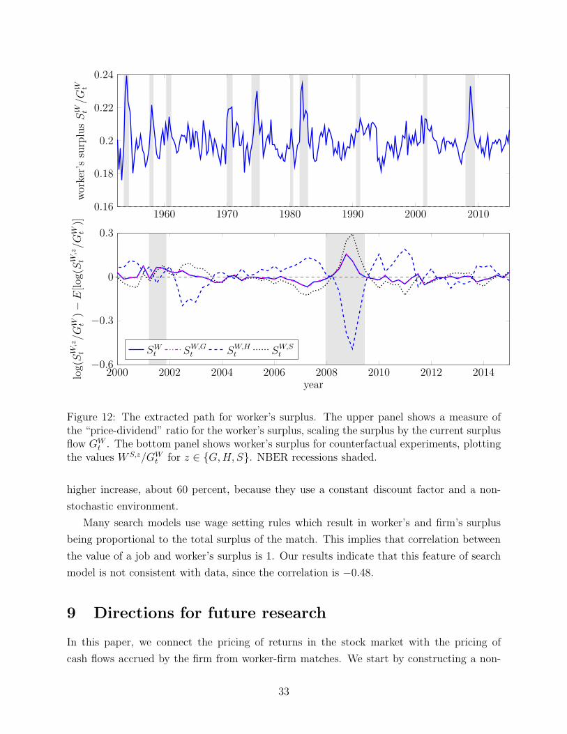
Figure 12 shows the extracted values for worker’s surplus. The mean value of quarterly

worker’s surplus is $1,030 (real 2009 dollars). This is rather small, and reflects the fact that

due to the high job-finding probability, being unemployed is not very costly.

Worker’s surplus is pro-cyclical, increasing sharply in downturns. Hence, recessions are

times when it is very valuable to have a job. Golosov and Menzio (2015) come to the same

conclusion, using a different methodology to evaluate worker’s surplus.

Worker’s surplus is again determined by three components, St, GWt and HW

t . To under-

stand the contribution of each of them to cyclicality of the surplus, we switch off fluctuations

in each of them separately and compute the surplus under these counterfactual scenarios.

This is the same type of decomposition we conducted with the value of the job. The bottom

panel of 12 depicts the results, focusing on the last two recessions. We use SW,xt to denote

surplus with constant growth rate in component x ∈{S,GW , HW

}.

Comparing SWt to other three SW,x

t , we see that H and S contribute greatly to the

volatility of the surplus, while cash flow GW does not. Indeed, worker’s surplus barely

changes if we turn off fluctuations in GW . This contrasts with the contribution of H which

is driven by the job-finding probability. Once we assume that it does not move over the

cycle, worker’s surplus SW,Ht actually decreases in recessions. Hence, the conclusion which

immediately emerges from this analysis is that the main reason for a high worker’s surplus in

recessions is the very low value of unemployment, driven down by a drop in the job-finding

rate.

Comparing SWt and SW,S

t , we see that stochastic discounting decreases worker’s surplus

in recessions. Ignoring stochastic discounting, we would conclude that worker’s surplus

has increased by 30 percent in the great recession, while taking stochastic discounting into

account, the increase is about half, 15 percent. Golosov and Menzio (2015) find an even

32

1960 1970 1980 1990 2000 20100.16

0.18

0.2

0.22

0.24worker’ssurplusSW t/G

W t

2000 2002 2004 2006 2008 2010 2012 2014−0.6

−0.3

0

0.3

year

log(S

W,z

t/G

W t)−E[log(S

W,z

t/G

W t)]

SWt SW,G

t SW,Ht SW,S

t

Figure 12: The extracted path for worker’s surplus. The upper panel shows a measure ofthe “price-dividend” ratio for the worker’s surplus, scaling the surplus by the current surplusflow GW

t . The bottom panel shows worker’s surplus for counterfactual experiments, plottingthe values W S,z/GW

t for z ∈ {G,H, S}. NBER recessions shaded.

higher increase, about 60 percent, because they use a constant discount factor and a non-

stochastic environment.

Many search models use wage setting rules which result in worker’s and firm’s surplus

being proportional to the total surplus of the match. This implies that correlation between

the value of a job and worker’s surplus is 1. Our results indicate that this feature of search

model is not consistent with data, since the correlation is −0.48.

9 Directions for future research

In this paper, we connect the pricing of returns in the stock market with the pricing of

cash flows accrued by the firm from worker-firm matches. We start by constructing a non-

33

parametric lower bound on two moments of the profit flow the firm receives from the marginal

worker that must be satisfied in order for the hiring Euler equation to hold. This weighted

variance bound, while conservative, is able to discriminate among theoretical models used in

the literature as well as among empirical proxies for the marginal profit flow. The bound is

constructed conditional on a model of a stochastic discount factor that prices financial assets

instrumented by a vector of variables that capture business-cycle variation in risk premia.

The properties of the profit flow and stochastic discount factor consistent with the bound

and returns on financial assets lead us to construct a parametric model from which we infer

fluctuations in the value of the worker to a firm. When constructed using inferred profit

processes consistent with the weighted variance bound, these fluctuations int he value of the

worker are able to match the business-cycle volatility of the unemployment rate.

Once we restrict the model of the stochastic discount factor to be consistent with the

Epstein–Zin recursive preference specification with a time-varying price of risk, and inform

the profit flow process using an empirical proxy, the ability of the model to generate em-

pirically observed fluctuations in the unemployment rates decreases, although it remains

substantial. We argue that the remaining wedge can be attributable to several factors, in-

cluding the discrepancy between the profit from the average and the marginal worker, as

well as shadow prices on financial constraints the firms are facing, relative to investors in

financial markets. A further study of the role of these constraints is left for future work.

Similarly, it would be interesting to study the implications of this weighted variance bound

for cross-sectional firm-level and industry-level data. If we interpret the wedge between the

bound and the moments measured using observed cash flows as the contribution of financial

constraints faced by different firms, then our framework allows to non-parametrically study

the distribution of these wedges across firms and industries, allowing us to measure the

cross-sectional heterogeneity in the impact of borrowing constraints for the unemployment

dynamics.

34

Appendix

A Derivation of the model

In this appendix, we derive the asset pricing implications for the model of household preferences.

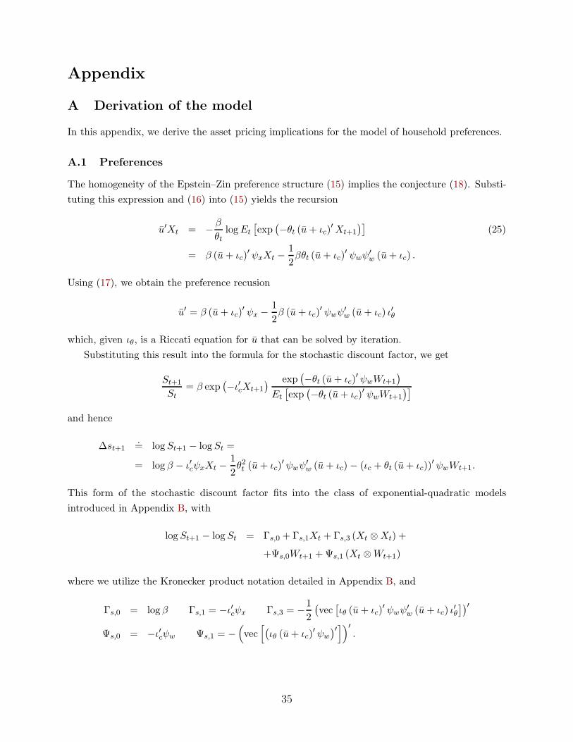
A.1 Preferences

The homogeneity of the Epstein–Zin preference structure (15) implies the conjecture (18). Substi-

tuting this expression and (16) into (15) yields the recursion

u′Xt = −β

θtlogEt

[exp

(−θt (u+ ιc)

′Xt+1

)](25)

= β (u+ ιc)′ ψxXt −

1

2βθt (u+ ιc)

′ ψwψ′

w (u+ ιc) .

Using (17), we obtain the preference recusion

u′ = β (u+ ιc)′ ψx −

1

2β (u+ ιc)

′ ψwψ′

w (u+ ιc) ι′

θ

which, given ιθ, is a Riccati equation for u that can be solved by iteration.

Substituting this result into the formula for the stochastic discount factor, we get

St+1

St= β exp

(−ι′cXt+1

) exp(−θt (u+ ιc)

′ ψwWt+1

)

Et

[exp

(−θt (u+ ιc)

′ ψwWt+1

)]

and hence

∆st+1.= log St+1 − log St =

= log β − ι′cψxXt −1

2θ2t (u+ ιc)

′ ψwψ′

w (u+ ιc)− (ιc + θt (u+ ιc))′ ψwWt+1.

This form of the stochastic discount factor fits into the class of exponential-quadratic models

introduced in Appendix B, with

logSt+1 − log St = Γs,0 + Γs,1Xt + Γs,3 (Xt ⊗Xt) +

+Ψs,0Wt+1 +Ψs,1 (Xt ⊗Wt+1)

where we utilize the Kronecker product notation detailed in Appendix B, and

Γs,0 = log β Γs,1 = −ι′cψx Γs,3 = −1

2

(vec[ιθ (u+ ιc)

′ ψwψ′

w (u+ ιc) ι′

θ

])′

Ψs,0 = −ι′cψw Ψs,1 = −(vec[(ιθ (u+ ιc)

′ ψw

)′

])′

.

35

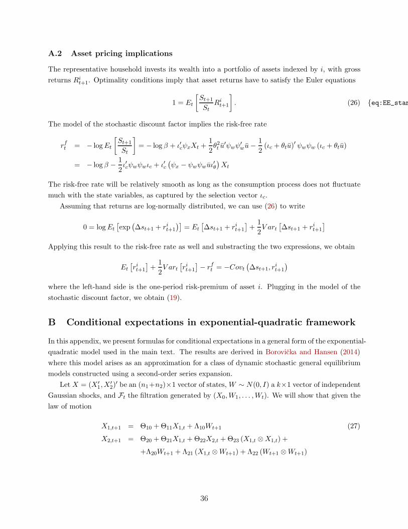
A.2 Asset pricing implications

The representative household invests its wealth into a portfolio of assets indexed by i, with gross

returns Rit+1. Optimality conditions imply that asset returns have to satisfy the Euler equations

1 = Et

[St+1

StRi

t+1

]. (26) {eq:EE_standard

The model of the stochastic discount factor implies the risk-free rate

rft = − logEt

[St+1

St

]= − log β + ι′cψxXt +

1

2θ2t u

′ψwψ′

wu−1

2(ιc + θtu)

′ ψwψw (ιc + θtu)

= − log β −1

2ι′cψwψwιc + ι′c

(ψx − ψwψwuι

′

θ

)Xt

The risk-free rate will be relatively smooth as long as the consumption process does not fluctuate

much with the state variables, as captured by the selection vector ιc.

Assuming that returns are log-normally distributed, we can use (26) to write

0 = logEt

[exp

(∆st+1 + rit+1

)]= Et

[∆st+1 + rit+1

]+

1

2V art

[∆st+1 + rit+1

]

Applying this result to the risk-free rate as well and substracting the two expressions, we obtain

Et

[rit+1

]+

1

2V art

[rit+1

]− r

ft = −Covt

(∆st+1, r

it+1

)

where the left-hand side is the one-period risk-premium of asset i. Plugging in the model of the

stochastic discount factor, we obtain (19).

B Conditional expectations in exponential-quadratic framework

In this appendix, we present formulas for conditional expectations in a general form of the exponential-

quadratic model used in the main text. The results are derived in Borovicka and Hansen (2014)

where this model arises as an approximation for a class of dynamic stochastic general equilibrium

models constructed using a second-order series expansion.

Let X = (X ′

1,X′

2)′ be an (n1+n2)×1 vector of states, W ∼ N(0, I) a k×1 vector of independent

Gaussian shocks, and Ft the filtration generated by (X0,W1, . . . ,Wt). We will show that given the

law of motion

X1,t+1 = Θ10 +Θ11X1,t + Λ10Wt+1 (27)

X2,t+1 = Θ20 +Θ21X1,t +Θ22X2,t +Θ23 (X1,t ⊗X1,t) +

+Λ20Wt+1 + Λ21 (X1,t ⊗Wt+1) + Λ22 (Wt+1 ⊗Wt+1)

36

and a process Mt = exp (Yt) whose additive increment is given by

Yt+1 − Yt = Γ0 + Γ1X1,t + Γ2X2,t + Γ3 (X1,t ⊗X1,t) + (28)

+Ψ0Wt+1 +Ψ1 (X1,t ⊗Wt+1) + Ψ2 (Wt+1 ⊗Wt+1) ,

we can write the conditional expectation of M as

logE [Mt | F0] =(Γ0

)t+(Γ1

)tX1,0 +

(Γ2

)tX2,0 +

(Γ3

)t(X1,0 ⊗X1,0) (29) {eq:em_app}

where(Γi

)tare constant coefficients to be determined.

The dynamics given by (27)–(28) embed as a special case the VAR specification of the Markov

dynamics. In this case the state vector Xt is represented by X1,t in (27), and the vector X2,t is

empty.

B.1 Definitions

To simplify work with Kronecker products, we define two operators vec and matm,n. For an m×n

matrix H, vec (H) produces a column vector of length mn created by stacking the columns of H:

h(j−1)m+i = [vec(H)](j−1)m+i = Hij .

For a vector (column or row) h of length mn, matm,n (h) produces an m× n matrix H created by

‘columnizing’ the vector:

Hij = [matm,n(h)]ij = h(j−1)m+i.

We drop the m,n subindex if the dimensions of the resulting matrix are obvious from the context.

For a square matrix A, define the sym operator as

sym (A) =1

2

(A+A′

).

Apart from the standard operations with Kronecker products, notice that the following is true. For

a row vector H1×nk and column vectors Xn×1 and Wn×1

H (X ⊗W ) = X ′ [matk,n (H)]′W

and for a matrix An×k, we have

X ′AW =(vecA′

)′

(X ⊗W ) .

Also, for An×n, Xn×1, Kk×1, we have

(AX)⊗K = (A⊗K)X

K ⊗ (AX) = (K ⊗A)X.

37

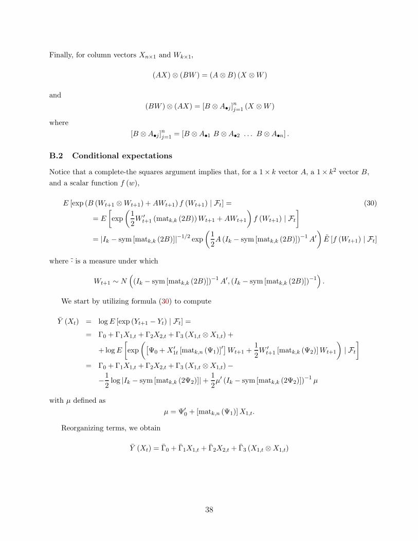
Finally, for column vectors Xn×1 and Wk×1,

(AX)⊗ (BW ) = (A⊗B) (X ⊗W )

and

(BW )⊗ (AX) = [B ⊗A•j ]nj=1 (X ⊗W )

where

[B ⊗A•j ]nj=1 = [B ⊗A•1 B ⊗A•2 . . . B ⊗A•n] .

B.2 Conditional expectations

Notice that a complete-the squares argument implies that, for a 1× k vector A, a 1× k2 vector B,

and a scalar function f (w),

E [exp (B (Wt+1 ⊗Wt+1) +AWt+1) f (Wt+1) | Ft] = (30)

= E

[exp

(1

2W ′

t+1 (matk,k (2B))Wt+1 +AWt+1

)f (Wt+1) | Ft

]

= |Ik − sym [matk,k (2B)]|−1/2 exp

(1

2A (Ik − sym [matk,k (2B)])−1A′

)E [f (Wt+1) | Ft]

where · is a measure under which

Wt+1 ∼ N((Ik − sym [matk,k (2B)])−1A′, (Ik − sym [matk,k (2B)])−1

).

We start by utilizing formula (30) to compute

Y (Xt) = logE [exp (Yt+1 − Yt) | Ft] =

= Γ0 + Γ1X1,t + Γ2X2,t + Γ3 (X1,t ⊗X1,t) +

+ logE

[exp

([Ψ0 +X ′

1t [matk,n (Ψ1)]′]Wt+1 +

1

2W ′

t+1 [matk,k (Ψ2)]Wt+1

)| Ft

]

= Γ0 + Γ1X1,t + Γ2X2,t + Γ3 (X1,t ⊗X1,t)−

−1

2log |Ik − sym [matk,k (2Ψ2)]|+

1

2µ′ (Ik − sym [matk,k (2Ψ2)])

−1 µ

with µ defined as

µ = Ψ′

0 + [matk,n (Ψ1)]X1,t.

Reorganizing terms, we obtain

Y (Xt) = Γ0 + Γ1X1,t + Γ2X2,t + Γ3 (X1,t ⊗X1,t)

38

where

Γ0 = Γ0 −1

2log |Ik − sym [matk,k (2Ψ2)]|+

1

2Ψ0 (Ik − sym [matk,k (2Ψ2)])

−1 Ψ′

0

Γ1 = Γ1 +Ψ0 (Ik − sym [matk,k (2Ψ2)])−1 [matk,n (Ψ1)] (31)

Γ2 = Γ2

Γ3 = Γ3 +1

2vec[[matk,n (Ψ1)]

′ (Ik − sym [matk,k (2Ψ2)])−1 [matk,n (Ψ1)]

]′

.

For the set of parameters P = (Γ0, . . . ,Γ3,Ψ0, . . . ,Ψ2), equations (31) define a mapping

P = E (P) ,

with all Ψj = 0. We now substitute the law of motion for X1 and X2 to produce Y (Xt) =

Y (Xt−1,Wt). It is just a matter of algebraic operations to determine that

Y (Xt−1,Wt) = logE [exp (Yt+1 − Yt) | Ft] =

= Γ0 + Γ1X1,t−1 + Γ2X2,t−1 + Γ3 (X1,t−1 ⊗X1,t−1)

+Ψ0Wt + Ψ1 (X1,t−1 ⊗Wt) + Ψ2 (Wt ⊗Wt)

where

Γ0 = Γ0 + Γ1Θ10 + Γ2Θ20 + Γ3 (Θ10 ⊗Θ10) (32)

Γ1 = Γ1Θ11 + Γ2Θ21 + Γ3 (Θ10 ⊗Θ11 +Θ11 ⊗Θ10)

Γ2 = Γ2Θ22

Γ3 = Γ2Θ23 + Γ3 (Θ11 ⊗Θ11)

Ψ0 = Γ1Λ10 + Γ2Λ20 + Γ3 (Θ10 ⊗ Λ10 + Λ10 ⊗Θ10)

Ψ1 = Γ2Λ21 + Γ3

(Θ11 ⊗ Λ10 +

[Λ10 ⊗ (Θ11)•j

]nj=1

)

Ψ2 = Γ2Λ22 + Γ3 (Λ10 ⊗ Λ10) .

This set of equations defines the mapping

P = E(P).

B.3 Iterative formulas

We can write the conditional expectation in (29) recursively as

logE [Mt | F0] = logE

[exp (Y1 − Y0)E

[Mt

M1| F1

]| F0

].

Given the mappings E and E , we can therefore express the coefficients P in (29) using the

39

recursion

Pt = E(P + E

(Pt−1

))

where the addition is by coefficients and all coefficients in P0 are zero matrices.

40

References

Bansal, Ravi, Dana Kiku, Ivan Shaliastovich, and Amir Yaron. 2014. Volatility, the Macroe-

conomy, and Asset Prices. Journal of Finance 69 (6):2471–2511.

Belo, Frederico, Xiaoji Lin, and Santiago Bazdresch. 2014. Labor Hiring, Investment

and Stock Return Predictability in the Cross Section. Journal of Political Economy

122 (1):129–177.

Bhandari, Anmol, Jaroslav Borovicka, and Paul Ho. 2016. Identifying Ambiguity Shocks in

Business Cycle Models Using Survey Data.

van Binsbergen, Jules, Wouter Hueskes, Ralph S.J. Koijen, and Evert B. Vrugt. 2013. Equity

Yields. Journal of Financial Economics 110 (3):503–519.

Borovicka, Jaroslav and Lars Peter Hansen. 2014. Examining Macroeconomic Models

through the Lens of Asset Pricing. Journal of Econometrics 183 (1):67–90.

Borovicka, Jaroslav, Lars Peter Hansen, Mark Hendricks, and Jose A. Scheinkman. 2011.

Risk-Price Dynamics. Journal of Financial Econometrics 9 (1):3–65.

Borovicka, Jaroslav, Lars Peter Hansen, and Jose A. Scheinkman. 2014. Shock Elasticities

and Impulse Responses. Mathematics and Financial Economics 8 (4):333–354.

Campbell, John Y. and John Cochrane. 1999. By Force of Habit: A consumption-based

explanation of aggregate stock market behavior. Journal of Political Economy 107 (2):205–

251.

Campbell, John Y. and Robert J. Shiller. 1988. The Dividend-Price Ratio and Expectations

of Future Dividends and Discount Factors. Review of Financial Studies 1:195–228.

Christiano, Lawrence J., Martin S. Eichenbaum, and Mathias Trabandt. 2015. Unemploy-

ment and Business Cycles. Forthcoming in Econometrica.

Dew-Becker, Ian. 2014. A Model of Time-Varying Risk Premia with Habits and Production.

Duke University.

Donangelo, Andres, Francois Gourio, and Miguel Palacios. 2016. The Cross-Section of Labor

Leverage and Equity Returns. May.

Epstein, Larry G. and Stanley E. Zin. 1989. Substitution, Risk Aversion, and the Temporal

Behavior of Consumption and Asset Returns: A Theoretical Framework. Econometrica

57 (4):937–969.

41

———. 1991. Substitution, Risk Aversion, and the Temporal Behavior of Consumption and

Asset Returns: An Empirical Analysis. The Journal of Political Economy 99 (2):263–286.

Favilukis, Hack and Xiaoji Lin. 2016. Wage Rigidity: A Quantitative Solution to Several

Asset Pricing Puzzles. Review of Financial Studies 29 (1):148–192.

Favilukis, Jack, Xiaoji Lin, and Xiaofei Zhao. 2015. The Elephant in the Room: The Impact

of Labor Obligations on Credit Risk.

Golosov, Mikhail and Guido Menzio. 2015. Agency Business Cycles.

Greenwald, Daniel L., Martin Lettau, and Sydney C. Ludvigson. 2014. Origins of Stock

Market Fluctuations.

Hagedorn, Marcus and Iourii Manovskii. 2008. The Cyclical Behavior of Equilibrium Unem-

ployment and Vacancies Revisited. American Economic Review 98 (4):1692–1706.

Hall, Robert E. 2017. High Discounts and High Unemployment. American Economic Review

107 (2):305–330.

Hall, Robert E. and Paul R. Milgrom. 2008. The Limited Influence of Unemployment on the

Wage Bargain. American Economic Review 98 (4):1653–1674.

Hansen, Lars Peter and Ravi Jagannathan. 1991. Implications of Security Market Data for

Models of Dynamic Economies. Journal of Political Economy 99 (2):225–262.

Hansen, Lars Peter and Thomas J. Sargent. 2015. Sets of Models and Prices of Uncertainty.

Working paper, University of Chicago and New York University.

Hansen, Lars Peter and Kenneth J. Singleton. 1982. Generalized Instrumental Variables

Estimation of Nonlinear Rational Expectations Models. Econometrica 50 (5):1269–1286.

Hansen, Lars Peter, John C. Heaton, and Erzo G. J. Luttmer. 1995. Econometrics Evaluation

of Asset Pricing Models. Review of Financial Studies 8 (2):237–274.

Kilic, Mete and Jessica A. Wachter. 2015. Risk, Unemployment, and the Stock Market: A

Rare-Events-Based Explanation of Labor Market Volatility.

Kozak, Serhiy. 2015. Dynamics of Bond and Stock Returns. University of Michigan.

Kozak, Serhiy and Shrihari Santosh. 2016. Linking Cross-Sectional and Aggregate Expected

Returns. University of Michigan and University of Maryland.

42

Kuehn, Lars-Alexander, Mikhail Simutin, and Jessie Jiaxu Wang. 2014. A Labor Capital

Asset Pricing Model.

Petrosky-Nadeau, Nicolas and Lu Zhang. 2013. Unemployment Crises. NBER Working

paper W19207.

Petrosky-Nadeau, Nicolas, Lu Zhang, and Lars-Alexander Kuehn. 2015. Endogenous Disas-

ters.

Shiller, Robert J. 1981. Do Stock Prices Move Too Much to be Justified by Subsequent

Changes in Dividends. American Economic Review 71 (3):421–436.

Shimer, Robert. 2005. The Cyclical Behavior of Equilibrium Unemployment and Vacancies.

American Economic Review 95 (1):25–49.

———. 2010. Labor Market and Business Cycles. Princeton University Press, Princeton,

NJ.

———. 2012. Reassessing the Ins and Outs of Unemployment. Review of Economic Dynamics

15 (2):127–148.

43