direct synchronous-asynchronous conversion system for ... · direct synchronous-asynchronous...

Direct Synchronous-Asynchronous Conversion System for

Hybrid Electrical Vehicle Applications. An Energy-Based

Modeling Approach

Raul-S. Munoz-Aguilar

Universitat Politecnica de Catalunya

Department of Electrical Engineering

08222 Terrassa, Spain

Email: [email protected]

Arnau Doria-Cerezo

Universitat Politecnica de Catalunya

Department of Electrical Engineering,

08800 Vilanova i la Geltru, Spain


Paul F. Puleston

IIF Marie Curie Fellow at IRI, CSIC-UPC, Barcelona, Spain.

Permanently, Researcher/Professor CONICET and LEICI,

National University of La Plata

1900 La Plata, Argentina


Abstract

This paper presents a proposal for a series hybrid electric vehicle propulsion system. This new configuration is

based on a wound-rotor synchronous generator (WRSM) and a doubly-fed induction machine (DFIM). The energy-

based model of the whole system is obtained taking advantage of the capabilities of the port-based modeling

techniques. From the dq port-controlled Hamiltonian description of the WRSM and DFIM, the Hamiltonian model

of the proposed Direct Synchronous-Asynchronous Conversion System (DiSAC) is developed. Subsequently, the

bond graph models of the DiSAC and associate systems are also provided. Numerical simulations are also presented

in order to validate the proposed system.

Index Terms

AC Machines, Hybrid Electric Vehicle, Modeling.

I. INTRODUCTION

Hybrid electrical vehicles (HEV) are the focus of many research interests because they are able to

provide good performance and long operating time [1] [2]. Basically, the HEV is composed of an internal

combustion engine, an electrical machine and a battery pack or ultracapacitor storage system [3]. The

main goal of this structure is to reduce the CO2 emissions by means of the regenerative breaking using

the electrical machine, both as a motor drive or as a generator, which charges or discharges the batteries.

It is also desired to keep the drivability performance of the vehicle [4]. Depending on the topology, HEV

can be divided into two basic configurations: parallel and series.

In this work we focus on the advanced topologies of series HEV. Wound-rotor electrical machines have

the ability to control them trough the rotor windings. It offers several advantages as the size of the power

converter could be smaller than a direct connection to the stator side.

The use of wound-rotor machines (as doubly-fed induction machines) has been studied as a part of

a power train [5] [6]. However, examples in [5] [6] had some performance limitations because they are

unable to control intermediate variables between both machines (power factor, reactive power or stator

voltage). More control inputs are necessary in order to achieve a good control for the HEV purposes

(for instance, the stator reactive power between both machines cannot be controlled with the previous

schemes). The propulsion system we propose consists of a wound-rotor synchronous generator (WRSM)

and a doubly-fed induction machine (DFIM), and it is an improved version of the topology proposed in

[7]. The main advantage of this configuration is the ability to manage the energy without a full power

converter between both machines. In this case the power management is done through the stator and

rotor voltages of the DFIM and the field voltage of the WRSM. This configuration of two machines with

wounded rotor allows to use smaller power converters than the conventional topology [4], also increasing

the number of control actions and, consequently, a better power management can be done.

Several modeling and simulation tools have been employed in this field [8] [9]. In particular, a powerful

modeling approach potentially suitable to deal with the inherent features of the proposed HEV system

is the one provided by network modeling. Network modeling is a prevailing trend in the description of

physical systems for analysis, control applications and simulation. The system is split into open subsystems

(tearing), the subsystems are modeled (zooming), and the model of the overall system is obtained by

interconnecting the models of the subsystems (linking) [10]. The main advantage of such approach is that

the models of the physical subsystems can be stored in libraries. The modeling process can be performed

in an iterative manner and the model of the overall system is simply constructed by interconnecting the

library sub-models.

Specifically, Energy-based modeling (EBM) is a network modeling technique which describes dynamical

systems from a physical point of view, representing the power flowing between the different elements

and where the energy is stored and dissipated. A recent implementation of this idea is known as port

Hamiltonian systems or port-controlled Hamiltonian systems (PCHS), see [11] and [12]. One of the

strong aspects of the PCHS is that a power-preserving interconnection between port-Hamiltonian sys-

tems results in another port-Hamiltonian system with composite energy, dissipation, and interconnection

structure. Based on this principle, complex, multidomain systems can be modeled by interconnecting

port-Hamiltonian descriptions of its subsystems.

PCHS theory provides the mathematical foundation of the bond graph approach, which allows to model

dynamical systems graphically, describing the energy flowing through different elements, which represents

source, storage, dissipative and transmission elements [13]. The bond graph description easily permits the

integration of submodels and, by means of a simple computer algorithm, the simulation-ready equations

TE

F

G P

B

M

(a) Serie

(a) Classic Series HEV scheme.

TE

F

DFIM

P B

IM

(b) Joint System

TE

F

PMSM DFIM

B P

(c) Variable Voltage Variable Fre-

quency

Figure 1. Classic and Advanced Series HEV schemes.

of a complex model can be derived.

In this paper, a new configuration for a HEV propulsion system is presented and the dynamical model

of the power train is obtained in the port-controlled Hamiltonian and bond graph descriptions. Finally,

some simulations are performed to evaluate the propulsion system under a standard driving test profile.

II. SYSTEM DESCRIPTION

A. State of the art

Figure 1(a) shows the classic configuration of a series HEV [4] [14]. It contains an internal combustion

engine (E), two electrical machines (G and M) connected by a power converter (P) which also is connected

to the batteries (B). Series HEV offers several advantages; the internal combustion engine (ICE) is

mechanically decoupled from the transmission, the final torque is given by an electrical machine and

also simple management strategies can be adopted [15], [16]. One of the disadvantages of this topology

is that all the power flows through the power converter and, consequently, the losses could be important.

Wound-rotor electrical machines offer the main advantage that the rotor voltages can be used for

control purposes. Based on this, some previous works proposed DFIM as electrical machines for HEV

applications [5][6], see Figures 1(b) and 1(c). The advantage of this kind of topologies is that a fractional

power converter converter can be used instead of a full power one. Effectively, the stator power converter is

replaced by a rotor power converter and, consequently, losses can be reduced. The so-called Joint System

[5] used a DFIM as generator, with an induction machine as a motor. In [6], the Variable Voltage Variable

Frequency scheme was introduced, with the DFIM as a motor with a permanent magnet synchronous

machine (PMSM) for the generating part.

B. The DiSAC propulsion system

However, the topologies presented in [5] and [6] are not able to control efficiently the system reactive

power and stator voltage amplitudes simultaneously. To overcome this drawback, a new topology for a

series HEV called Direct Synchronous-Asynchronous Conversion System (DiSAC) is introduced in this

paper.

WRSM

τE ,ω

DFIMvs,is

τ,ωr

vI ,iI

AC

DCvF ,iF vr,ir

BDC

ACDC

DC

Figure 2. Electrical scheme of the DiSAC system.

Figure 2 shows the electrical connection of the DiSAC system. The WRSM is mechanically connected

with the ICE, and operates as a generator. The WRSM and DFIM stators are directly connected one to the

other and the shaft of the DFIM is coupled to the HEV transmission. Notice that the DFIM can operate

either in generator or motor mode. Both machines (WRSM and DFIM) are rotor connected to the batteries

by means of DC/DC and AC/DC converters, respectively, and batteries are also connected to the stator

side by means of a power converter.

This new scheme defines six control inputs: the field (or rotor) voltage of the WRSM, vF , the two rotor

PmDPmW PsDPsW

PI

Pbat

PrPF

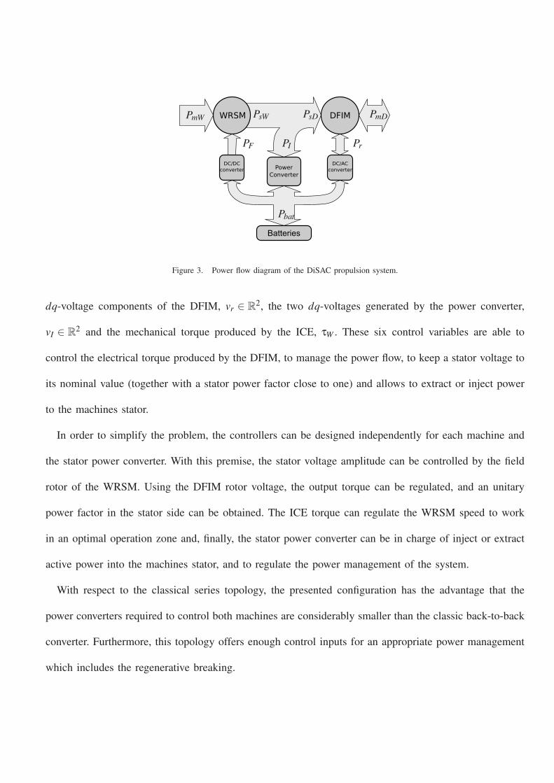
Figure 3. Power flow diagram of the DiSAC propulsion system.

dq-voltage components of the DFIM, vr ∈ R2, the two dq-voltages generated by the power converter,

vI ∈ R2 and the mechanical torque produced by the ICE, τW . These six control variables are able to

control the electrical torque produced by the DFIM, to manage the power flow, to keep a stator voltage to

its nominal value (together with a stator power factor close to one) and allows to extract or inject power

to the machines stator.

In order to simplify the problem, the controllers can be designed independently for each machine and

the stator power converter. With this premise, the stator voltage amplitude can be controlled by the field

rotor of the WRSM. Using the DFIM rotor voltage, the output torque can be regulated, and an unitary

power factor in the stator side can be obtained. The ICE torque can regulate the WRSM speed to work

in an optimal operation zone and, finally, the stator power converter can be in charge of inject or extract

active power into the machines stator, and to regulate the power management of the system.

With respect to the classical series topology, the presented configuration has the advantage that the

power converters required to control both machines are considerably smaller than the classic back-to-back

converter. Furthermore, this topology offers enough control inputs for an appropriate power management

which includes the regenerative breaking.

C. Power flow operation

The power flow operation is illustrated in Figure 3. Thanks to the use of wounded electrical machines,

the power is mainly flowing through the WRSM, the DFIM and the power inverter, and the energy required

by the fractional DC/DC and AC/DC converters is relatively small, see simulation results in Section VI.

The WRSM only acts as a generator with a mechanical incoming power, PmW , and provides an electrical

power, PsW . Both are related by

PmW = PsW −RsW |isW |2 −BW ω2W (1)

were the terms RsW |isW |2 and BW ω2W represents the ohmic and mechanical losses. The field power required

is

PF = RF i2F . (2)

Similarly to the WRSM, the DFIM stator power flows are given by

PsD = PmD −RsD|isD|2 −BDω2

D (3)

where PsD is the power flowing through the stator side, PmD is the delivered mechanical power, and

RsD|isD|2, BDω2

D represents the ohmic and mechanical losses. The DFIM rotor power is

Pr = (ωs −ωD)τD −Rr|ir|2, (4)

where the Rr|ir|2 term are the ohmic losses. Notice that Pr strongly depend on the slip. So, to reduce it,

it would be desirable to regulate the WRSM speed, ωs close to ωD keeping the ICE within the range

allowing to have the higher efficiency. See further details of the power analysis in [17].

In a regenerative breaking mode, the kinetic energy recovered flows from the DFIM to the batteries

through the power converter.

III. PORT CONTROLLED HAMILTONIAN MODEL

In this section, the port-controlled Hamiltonian model of the proposed series HEV DiSAC configuration

is derived interconnecting the standard dq models of the DFIM, WRSM and the inverter with a battery

model by means of power converters.

Hamiltonian modeling uses state dependent energy functions to characterize the dynamics of the different

subsystems, and connects them using a Dirac structure, which embodies the power preserving network of

relationships established by the corresponding physical laws. The result is a mathematical model with a

specific structure, called port-controlled Hamiltonian system (PCHS) [11], which lends itself to a natural,

physics-based analysis and control design.

An explicit PCHS has the form

x = (J (x)−R (x))∂H +G (x)u

y = G T (x)∂H

(5)

where x ∈Rn are the energy variables (or state vector), u,y ∈R

m are the port variables, and H(x) : Rn →R

is the Hamiltonian function, representing the energy function of the system. The ∂x (or ∂, if no confusion

arises) operator defines the gradient of a function of x and, in the sequel, we will take it as a column vector.

J (x) ∈ Rn×n is the interconnection matrix, which is skew-symmetric (J (x) = −J (x)T ), representing the

internal energy flow in the system, and R (x) ∈Rn×n is the dissipation matrix, symmetric and, in physical

systems, positive semidefinite (R (x) = R (x)T ≥ 0), which accounts for the internal losses of the system.

Finally, G (x) ∈ Rn×m is an interconnection matrix describing the port connection of the system to the

outside world. It yields the flow of energy to/from the system through the port variables, u and y, which

are conjugated, i.e. their dot product has units of power.

Usually, three-phase electrical machine modeling uses the so-called Park (or dq) transformation. This

mathematical transformation allows to decouple variables and to facilitate the solution of difficult equations

which depends on the rotor position [18]. With the dq transformation the abc three-phase variables

(voltages and currents) are reduced to a two-phase dq variables (assuming that the homopolar component

is equal to zero due to the existence of a balanced system). The reference frame for the Park transformation

depends on the application.

In this case, the selected reference is the mechanical angle of the WRSM. In the sequel, machines of

one pair of poles are considered. Note that in such case the mechanical speed of the synchronous machine,

ωW , matches the stator frequency, ωs.

A. PCHS of a doubly-fed induction machine

The PCHS of a doubly-fed induction machine has been presented in [19]. The dynamics is given by

xD = (JD(x)−RD)∂HD +GDuD. (6)

The Hamiltonian variables are

xTD = [λT

sD,λTr , pD],

where λsD = [λsDd,λsDq]T and λr = [λrd,λrq]

T are the stator and rotor fluxes in dq-coordinates, respectively,

pD = JDωD is the mechanical momentum, ωD is the mechanical speed and JD is the inertia of the rotating

parts. The D subindex has been included to refer to the DFIM.

The interconnection and damping matrices are, respectively,

JD(x) =

−ωsLsDJ2 −ωsLsrJ2 0

−ωsLsrJ2 −(ωs −ωD)LrJ2 LsrJ2isD

0 LsriTsDJ2 0

RD =

RsDI2 0 0

0 RrI2 0

0 0 BD

where isD, ir ∈ R2 are the stator and rotor currents, R and L are resistance and inductances1, ωs is the

stator electric frequency, BD is the mechanical damping, and

J2 =

0 −1

1 0

, I2 =

1 0

0 1

.

To simplify the notation, 0 represents a zero matrix with the appropriate dimension.

Considering that all the elements are linear, Hamiltonian variables (fluxes and momentum) are related

with currents and mechanical speed by

xD = LD

isD

ir

ωD

(7)

where

LD =

LsDI2 LsrI2 0

LsrI2 LrI2 0

0 0 JD

.

The port connection, GD, is 5×5 identity matrix, with the port variables uTD = [vT

sD,vTr ,τD], where vsD,vr ∈

R2 are the stator and rotor voltages and τD is an external torque. The Hamiltonian model is completed

with the energy function

HD(xD) =1

2xT

DL−1D xD.

Notice that the variables obtained operating ∂HD is a vector with the stator and rotor currents and the

mechanical speed.

B. PCHS of a wound-rotor synchronous machine

A Port-controlled Hamiltonian model of a synchronous machine with permanent magnets, can be

found in [20]. However, the wound rotor synchronous machine includes a rotor winding which has to be

1Subscripts s and r refer to stator and rotor respectively.

considered. Then, the PCHS is

xW = (JW (x)−RW )∂HW +GW uW , (8)

with

xTW = [λT

sW ,λF , pW ],

where λsW = [λsWd,λsWq]T is the stator inductor flux in dq-coordinates, λF is the rotor (or field) inductor

flux, pW = JW ωW is the mechanical momentum, ωW is the mechanical speed, and JW is the inertia of the

rotating parts. In this case, the W subindex has been included to refer to the WRSM.

The interconnection and damping matrices are, respectively,

JW =

−ωW LsW J2 0 −MiF

0 0 0

MT iF 0 0

RW =

RsW I2 0 0

0 RF 0

0 0 BW

where isW ∈ R2 are the stator currents, iF is the rotor (or field) current, R and L are resistance and

inductances2, BW is the mechanical damping and

M =

0

Lm

with Lm being the mutual inductance.

2Subscripts s and F refer to stator and field respectively.

Similarly to the DFIM, for a linear case the WRSM fluxes and momentum are related with currents

and mechanical speed by

λW = LW

isW

iF

ωW

(9)

and the inductance matrix, LW , is

LW =

LsW I2 M 0

MT LF 0

0 0 JW

.

The port connection, GW , is represented by an identity 4 × 4 matrix, with the port variables uTW =

[vTsW ,vF ,τW ], where vsW ∈ R

2 is the stator voltages, vF is the rotor (or field) voltage, and τW is the

applied external torque. Finally, the Hamiltonian function is

HW (xW ) =1

2xT

WL−1W xW .

C. PCHS of a three-phase DC/AC inverter

As a first approximation, and neglecting the effect of switches, the three-phase DC/AC inverter can be

modeled as a couple of voltage sources in series with an RL element. Then, the PCHS takes the form

xI = (J I −R I)∂HI +G IuI, (10)

where the state are the inductor fluxes xTI = [λId,λIq] ∈ R

2. The interconnection matrix reflects the effect

of the rotation in the Park coordinates

J I =−ωILIJ2,

where ωI is the frequency of the generated AC voltage, LI is the inductance parameter, and the losses

corresponds to the parasitic resistive effects contained in the dissipation matrix

R I = RII2.

The port variables, uTI = [eT

I ,vTI ], comprise the generated voltages by the switching policy, eT

I = [eId,eIq]∈

R2, and the inverter voltages, vT

I = [vId,vIq] ∈ R2, which are connected to the dynamics with

G I =

[

I2 I2

]

. (11)

Fluxes are defined as

xI = LIiI,

where iTI = [iId, iIq] ∈ R2 are the inductor currents. The Hamiltonian function is

HI(xI) =1

2xT

I L−1I xI.

D. PCHS of a battery

A battery (lead-acid or lithium-ion, among others) is an energy storage device which involves electro-

chemical reactions and complex dynamics [4]. In this paper, a simplified model of a battery is adopted

which, thanks to the network modeling basis of the PCHS, can be easily replaced by a complex model if

necessary.

The battery model consists of a nonlinear capacitor in parallel with a resistance, yielding a first order

nonlinear system, which can be represented in a PCHS form with

xB =−RB∂HB +GBuB (12)

where xB = qB is the state of charge (SOC), RB models the self-discharge, GB = b1 scales the charge to

p.u. (or percent units, depending on the used model), and the input corresponds to the incoming current,

uB = iB. Note that, as the battery is a one-dimensional system, the interconnection matrix is null, JB = 0.

The Hamiltonian function,

HB =1

4b2(xB −b3)

4 +b4xB (13)

0 0.2 0.4 0.6 0.8 1 1.2 1.4375

380

385

390

395

400

405

410

415

SOC

vB

Figure 4. The SOC vs. battery voltage.

where xB > 0, contains the nonlinear relationship between the SOC and the battery voltage, vB, by means

of the output equation

yB = GB∂HB (14)

where yB = vB. From the latter, the SOC and the voltage battery are related by

vB = b2(xB −b3)3 +b4. (15)

Figure 4 shows the battery voltage versus the SOC (15) , with the following parameters b2 = 100,

b3 = 0.7 and b4 = 400. Realistic approximations to an industrial battery can be obtained modifying the

Hamiltonian function (13), or interconnecting several cell models.

E. The overall system

The whole system is obtained linking the aforementioned subsystems. Figure 2 shows how they are

interconnected. The machines are connected through the stator windings together with the power converter.

Then, the link of the DC/AC power converter and the electrical machines subsystems is achieved by setting

the Kirchhoff voltage law

vsD = vsW = vI, (16)

and the Kirchhoff current law,

isD + isW + iI = 0. (17)

Also, the interconnection implies a common frequency,

ωs = ωW = ωI. (18)

Also, the rotor windings of both WRSG and DFIM, and the inverter, are connected to the battery

by means of power converters that manage the power flowing through the system. Power converters are

modeled as ideal switches that relate the voltages and currents as follows

vF = µW vB (19)

iBW = µW iF (20)

vr = µDvB (21)

iBD = µTDir (22)

eI = µIvB (23)

iBI = µTI iI (24)

where µW is the switch position of the DC-DC power converter, µD,µI ∈ R2 are the switching policy of

the DC-AC inverters in the dq-coordinates (see examples in [21]), and iBW , iBD, iBI are the currents in the

battery side of the power converters that are related with the battery current by

iB =−(iBD + iBW + iBI). (25)

Using (20), (22) and (24) in (25) and the Hamiltonan functions HW , HD and HI

iB =−ΓTD∂HD −ΓT

W ∂HW −µTI ∂HI, (26)

where ΓTD = [0,µT

D,0] ∈ R5 and ΓT

W = [0,µW ,0] ∈ R4. Similarly with (19), (21), (23) and HB

vF = µW ∂HB (27)

vr = µD∂HB (28)

eI = µI∂HB. (29)

This leads to the PCHS

xD

xW

xI

xB

=

JD(xD)−RD 0 0 ΓD

0 JW (xW )−RW 0 ΓW

0 0 J I −R I µI

−ΓTD −ΓT

W −µTI −RB

∂HD

∂HW

∂HI

∂HB

+B vI +G cu (30)

with the external connection matrix,

GTc =

0 0 1 0 0 0 0 0

0 0 0 0 0 1 0 0

∈ R2×12

, (31)

the input port variables uT = [τD,τW ] ∈ R2, and the interconnection voltage constrain (16) is denoted in

BT =

[

I2 0 0 I2 0 0 I2 0

]

∈ R2×12

, (32)

Note that the constraint on the currents (17), is represented by

0 = B T

∂HD

∂HW

∂HI

∂HB

. (33)

The internal constraint voltage can be eliminated as follows. Let B ⊥ denote a full-rank left annihilator3

of B ,

3In general, a full-rank left annihilator of B ∈ Rn×m, B ⊥, implies: B ⊥B = 0 and rank(B ⊥) = n−m.

B⊥ =

I2 0 0 0 0 0 −I2 0

0 I2 0 0 0 0 0 0

0 0 1 0 0 0 0 0

0 0 0 I2 0 0 −I2 0

0 0 0 0 1 0 0 0

0 0 0 0 0 1 0 0

0 0 0 0 0 0 0 1

. (34)

Hence, premultiplying (30) with B ⊥, and taking into account that the first and last dynamics are the

same, the whole dynamics take the PCHS form

x = (J (x)−R )∂H +G u (35)

with the new state defined by

xT = [λTDI,λ

Tr , pD,λ

TIW ,λF , pW ,qB],

where λDI = λsD−λI and λWI = λsW −λI . The interconnection and dissipation matrices are (39) and (40),

respectively, the energy function is the sum of HD, HW , HI , and HB, that can be written as

H(x) =1

2λTL−1λ+

1

2J−1

D p2D +

1

2J−1

W p2W +HB(qB), (36)

where λT = [λTDI,λ

Tr ,λ

TIW ,λF ],

L =

(LsD +LI)I2 LsrI2 LII2 0

LsrI2 LrI2 0 0

LII2 0 (LsW +LI)I2 M

0 0 MT LF

(37)

and the external connection matrix is

GT =

0 0 1 0 0 0 0

0 0 0 0 0 1 0

. (38)

J (x) =

−ωs(LsD +LI)J2 −ωsLsrJ2 0 0 0 0 −µI

−ωsLsrJ2 −(ωs −ωD)LrJ2 LsrJ2isD 0 0 0 µD

0 LsriTsDJ2 0 0 0 0 0

0 0 0 −ωs(LsW +LI)J2 0 −MiF −µI

0 0 0 0 0 0 µW

0 0 0 MT iF 0 0 0

µTI −µT

D 0 µTI −µW 0 0

(39)

R =

(RsD +RI)I2 0 0 RII2 0 0 0

0 RrI2 0 0 0 0 0

0 0 BD 0 0 0 0

RII2 0 0 (RsW +RI)I2 0 0 0

0 0 0 0 RF 0 0

0 0 0 0 0 BW 0

0 0 0 0 0 0 RB

(40)

As expected when modeling power converters in the port-controlled Hamiltonian framework, the switch-

ing control actions (µD, µW and µI) appear in the interconnection matrix (39), see [22] for further details.

IV. BOND GRAPH MODEL

Many electrical machines are described using the bond graph approach. From the DC machine [13] or

AC generator [23], to three-phase induction machines [21][24]. HEV are also modelled using this graphic

tool. In [25] a complete bond graph model for a long urban transit bus is obtained and simulated. A

LlsD : I Lsr : I Llr : I

R : RsD R : Rr

Se : VsdD 1 0 1 Se : Vrd R : BD

GY : ωsLsr MGY : LsrisqD + Lrirq

GY : ωsLsD GY : ωsLr 1 Se : τD

GY : ωsLsr MGY : LsrisdD + Lrird

Se : VsqD 1 0 1 Se : Vrq I : JD

R : RsD R : Rr

LlsD : I Lsr : I Llr : I

Figure 5. Bond graph model of a doubly-fed induction machine.

bond graph model of a parallel HEV system is presented in [26]. In that case, the electrical machine

and internal combustion engine were modelled as an ideal torque sources (Se-element), while the main

contribution was focused in the transmission, aerodynamics and wheel models.

Exploiting the network based modeling of the bond graph approach, the whole model of the proposed

series HEV DiSAC configuration is obtained by linking the different subsystems.

The bond graph models of the DFIM, the WRSM and the power converter are depicted in Figures 5,

6 and 7, respectively. For these models the following I-elements LlsD, Llr, LlsW , LlF are defined as

LlsD = LsD −Lsr

Llr = Lr −Lsr

LlsW = LsW −Lm

LlF = LF −Lm.

The battery is modeled as a nonlinear capacitor with a resistance emulating the self-discharge property,

see in Figure 8 the corresponding bond graph. A complex models of batteries can be found in the

literature, see examples in [27] and [28] for lead-acid and lithium-ion batteries, respectively. Both can be

used, directly replacing the bong graph of Figure 8.

LlsW : I Lm : I LlF : I

R : RsW R : RF

Se : VsdW 1 0 1 Se : VF R : BW

MGY : ωsLsW 1 Se : τW

Se : VsqW 1 MGY : LmiF I : JW

R : RsW

LsW : I

Figure 6. Bond graph model of a wound-rotor synchronous machine.

Se : eId

LI : I 1 R : RI

Se : vId MGY : ωsLI Se : vIq

LI : I 1 R : RI

Se : eIq

Figure 7. Bond graph model of the stator inverter.

Linking the WRSM, the DFIM and the DC-AC inverter through the stator side of both machines,

and connecting the battery by means of the DC-DC and DC-AC power converters, the whole model is

obtained, see Figure 9. In this case, power converters are modeled as a modulated transformer, MTF, which

represents de averaged duty-cycle of the switches, [29]. Also, multi-bonds are used for the dq-coordinates

R : RB

S f : iB 0

C : ∂HB

Figure 8. Bond graph model of the battery.

Se : τW WRSG 0 DFIM Se : τD

MT F : µW INV ERT ER MT F : µD

MT F : µI

0

BAT ERIES

Figure 9. Bond graph model of the complete system.

in order to simplify the bond graph.

As a consequence of linking the power converter with the WRSM and the DFIM the I-elements of

the stator inverter, in Figure 7, are now with a non-preferred causality. This corresponds to the current

constraint given by (33).

V. VEHICLE MODEL

The DiSAC power train system is tested as a propulsion system for an HEV. To this end, the bond

graph model of the DiSAC system can be connected to the vehicle dynamics through the mechanical

port of the DFIM. As mentioned above, the bond graph technique is specially attractive for linking easily

different subsystems.

Froll

Fslo

Θ

FP

Figure 10. Vehicle simplified model

The vehicle dynamics is modeled as a mass, M, subjected to different forces, see Figure 10. As a first

approach there are considered the propulsion force, FP, the effects associated with the rolling resistance,

Froll =CMgv, (41)

and with the slope of the road,

Fslo = MgsinΘ, (42)

where C is the coefficient of the rolling resistance, g is the gravitational acceleration, v is the vehicle speed

and Θ is the road angle measured with respect to the horizontal. This model can be improved considering

the aerodynamic drag and the wheel bearing losses [30].

Furthermore, there are considered the transformation from the angular dynamics to the translational

one (which depends on the radius of the wheels, r) and the vehicle transmission, rtrans, which scales the

torque and speed through the differential and the transmission ratio and is considered lossless.

The bond graph of the vehicle dynamics is depicted in Figure 11. It consists in a I-element (with the

mass of the vehicle), a dissipative R-element, which models the rolling resistance, and an external Se-

source with the gravitational effect in case of certain slope of the road. The two TF-elements model the

transformation from the angular dynamics (the wheels) and the transmission and differential ratio.

I : M

Se : τP T F : rtrans T F : r 1 Se : MgsinΘ

R : CMg

Figure 11. Bond graph model of the vehicle dynamics.

The complete system for simulation purposes, which includes the DiSAC power train with the vehicle

dynamics is obtained by linking the bond graph in Figures 9 and 11 trough the bonds corresponding to

the torque of the DFIM and the vehicle, τD and τP, respectively.

VI. SIMULATION RESULTS

In this Section numerical simulations are presented in order to test the proposed power train. The

WRSM was controlled via a PI controller. The DFIM uses a current PI controller, designed accordingly

to [31]. A PI control outer loop emulates the driver action and provides the torque reference to track the

desired speed.The stator inverter is also controlled via a PI loop. Simulations were performed using the

20sim software which contains a bond graph editor.

The machines rated power are PW = 8.1kVA and PD = 15kVA. The DFIM and WRSM parameters

are RsD = 0.2147Ω, Rr = 0.2205Ω, Ls = 65.181mH, Lr = 65.181mH, Lsr = 64.19mH, JD = 0.102Kgm2,

BD = 0.009541Nmrad−1s−1, and LsW = 113.127mH, RsW = 1.62Ω, Lm = 108.6mH, LF = 109.92mH,

RF = 1.208H and the WRSM mechanical speed is fixed at ω = 314rad s−1. The stator inverter inductance

is set to LI = 4mH with a parasitic resistor of RI = 0.1Ω. The transmission and differential ratio are set

to 1 and 4, respectively. The battery parameters are: b1 = 0.1, b2 = 1 ∗ 10−6, b3 = 0.9, and b4 = 700.

The control parameters are Kp = 20, Ki = 3 (for the WRSM) and Kp = 1, Ki = 0.01 (DFIM). The speed

control parameters are Kp = 10 and Ki = 0.05. Finally, the stator power converter control gain parameters

are Kp = 0.1, Ki = 1.

The control objectives are to regulate the stator voltage (V = 400V), the WRSM output power (Ps =

3kW ), the DFIM mechanical speed (ωr), and to keep an unitary DFIM stator power factor. Several reference

speed changes, namely, increase and decrease reference speed at low, medium and high speed, have been

set in order to show the different power flow conditions.

Figures 12, 14, 16, 18, 20, 22, 24 and 26 show in the upper the DFIM mechanical speed and its

reference (both were referenced to machine speed, for this reason the unities are rad s−1); in the middle

the stator voltage amplitude and in the bottom the DFIM stator power factor (PF).

Figures 13, 15, 17, 19, 21, 23, 25 and 27 show the electrical power flow trough the DFIM stator side,

PsD, SM stator windings, PsW , and the inverter, PI4. As explained before, the rotor active power changes

is bidirectional and allows to store energy into the batteries. In this case the battery state of charge (SOC)

is not taken into account. For further development when the battery reaches to the maximum allowed

SOC, either, an electrical or mechanical brake must exist.

Figures from 12 to 19 represent the system behavior at low speed, while Figures from 20 to 23 and

from 24 to 27 represent them for medium and high speed, respectively. The speed reference changes were

extracted from the NEDC (New European Driving Cycle) profile.

As a result, note how the control objectives are reached and the power flow through the proposed

DiSAC system can be controlled. In this work a power limit was not imposed to the stator converter,

neither absorbing nor providing power. In future works this power limitations will be studied, together

with the power ratio of each converter The control design is also a future study case.

Note that the DFIM stator PF remains close to ±1 when the stator power of the DFIM is positive or

negative, respectively (i.e., when the machine is providing power to the wheels or it is in regenerative

braking). When the vehicle is stopped PF=0 due to the magnetization losses.

In Figure 13 the DFIM accelerates from zero to low speed. The inverter starts absorbing approximately

the amount of power generated by WRSM, while the power consumed by the DFIM is close to zero.

Subsequently, after the transient, the DFIM absorbs the power provided by both the inverter and the

WRSM. Figure 19 corresponds to the case in which the machine decelerates from low speed to zero.

The result of the DFIM accelerating at low speed is presented in Figure 15. The inverter starts providing

electrical power from the batteries, while the DFIM absorbs such power together with the one generated

by the WRSM. After the transient, at constant speed, the power consumed by the DFIM is lower than

the power generated by the WRSM. Note that the extra amount of power is absorbed by batteries trough

the inverter. Figure 17 corresponds to the case in which the machine decelerates at low speed.

4In the dq coordinates, the instantaneous active and reactive power can be computed as Pr = vTr ir and Qs = vT

s J2is.

0 0.2 0.4 0.6 0.8 1 1.2 1.4 1.6 1.8 20

20

40

60

ωr,

ωre

f [ra

d/s

]

time [s]

ωr

ωref

0 0.2 0.4 0.6 0.8 1 1.2 1.4 1.6 1.8 2350

400

450

V [V

]

time [s]

0 0.2 0.4 0.6 0.8 1 1.2 1.4 1.6 1.8 2

−1

−0.5

0

0.5

1

cos(φ

)

time [s]

Figure 12. Simulation results: DFIM mechanical speed and its reference, Stator voltage amplitude (V ) and Stator Power Factor.

Figures 21 and 23 present the acceleration and deceleration of DFIM at medium speed, respectively.

During the acceleration, the batteries provides the extra power consumption of the DFIM, whereas at

constant speed the batteries stores the extra power generated by the WRSM, the deceleration process is

complementary.

Finally, Figures 25 and 27 present the acceleration and deceleration of DFIM at high speed, respectively.

At this speed, the power consumption of the DFIM is very high either at constant speed or accelerating,

then, both the WRSM and the batteries provide all the energy. On the other hand, during the decelerating

part, the energy is stored into the batteries.

In optimal conditions, the SOC can be regulated by adjusting the WRSM generated power, but it is out

of the scope of this paper and it will be studied in future works.

VII. CONCLUSIONS

An alternative architecture for a series HEV propulsion system has been proposed. It is composed by

two wounded rotor machines (WRSM and DFIM) directly connected through the stator, with a DC/AC

converter. The advantage of this topology is that the required power converters are smaller than other

2 2.2 2.4 2.6 2.8 3 3.2 3.4 3.6 3.8 42

2.5

3

3.5

4

PW

[kW

]

2 2.2 2.4 2.6 2.8 3 3.2 3.4 3.6 3.8 4−20

−10

0

10

20

PD

[kW

]

2 2.2 2.4 2.6 2.8 3 3.2 3.4 3.6 3.8 4−20

−10

0

10

20

Pin

v [kW

]

time [s]

Figure 13. Simulation results: WRSM (PW ), DFIM (PD) and stator converter (Pinv) electrical powers

0 0.2 0.4 0.6 0.8 1 1.2 1.4 1.6 1.8 20

20

40

60

ωr,

ωre

f [ra

d/s

]

time [s]

ωr

ωref

0 0.2 0.4 0.6 0.8 1 1.2 1.4 1.6 1.8 2350

400

450

V [V

]

time [s]

0 0.2 0.4 0.6 0.8 1 1.2 1.4 1.6 1.8 2

−1

−0.5

0

0.5

1

cos(φ

)

time [s]


series configurations [4].

The complex system under study has been divided into several subsystems; the WRSM, the DFIM the

power inverter, the batteries and the required DC-DC and DC-AC power converters. Two energy-based

models have been presented, following the Hamiltonian formalism and the bond graph approach, and

the whole system is obtained by linking the submodels. As additional feature, the submodel integration

capability, inherent to bond graph technique, allows to easily expand the proposed model, by intercon-

0 0.2 0.4 0.6 0.8 1 1.2 1.4 1.6 1.8 22

2.5

3

3.5

4

PW

[kW

]

0 0.2 0.4 0.6 0.8 1 1.2 1.4 1.6 1.8 2−20

−10

0

10

20

PD

[kW

]

0 0.2 0.4 0.6 0.8 1 1.2 1.4 1.6 1.8 2−20

−10

0

10

20

Pin

v [kW

]

time [s]


0 0.2 0.4 0.6 0.8 1 1.2 1.4 1.6 1.8 20

20

40

60

ωr,

ωre

f [ra

d/s

]

time [s]

ωr

ωref

0 0.2 0.4 0.6 0.8 1 1.2 1.4 1.6 1.8 2350

400

450

V [V

]

time [s]

0 0.2 0.4 0.6 0.8 1 1.2 1.4 1.6 1.8 2

−1

−0.5

0

0.5

1

cos(φ

)

time [s]


nection with other mechanical (transmission, wheels, aerodynamics...) and electrical parts (discrete power

converters, complex battery models,...), in future works. Moreover, from a control viewpoint, the presented

PCH model will be of great help to design passivity-based controllers.

The proposed models of the novel series HEV topology has been comprehensively assessed through

simulations, showing satisfactory results. The proposed DiSAC system can be fully controlled.

Future works include the control design for the different system stages and the energy management

0 0.2 0.4 0.6 0.8 1 1.2 1.4 1.6 1.8 22

2.5

3

3.5

4

PW

[kW

]

0 0.2 0.4 0.6 0.8 1 1.2 1.4 1.6 1.8 2−20

−10

0

10

20

PD

[kW

]

0 0.2 0.4 0.6 0.8 1 1.2 1.4 1.6 1.8 2−20

−10

0

10

20

Pin

v [kW

]

time [s]


0 0.2 0.4 0.6 0.8 1 1.2 1.4 1.6 1.8 20

20

40

60

ωr,

ωre

f [ra

d/s

]

time [s]

ωr

ωref

0 0.2 0.4 0.6 0.8 1 1.2 1.4 1.6 1.8 2350

400

450

V [V

]

time [s]

0 0.2 0.4 0.6 0.8 1 1.2 1.4 1.6 1.8 2

−1

−0.5

0

0.5

1

cos(φ

)

time [s]


policy of the whole system.

VIII. ACKNOWLEDGMENTS

R. S. Munoz-Aguilar, A. Doria-Cerezo and P.F. Puleston were partially supported by the Spanish

government research projects ENE2011-29041-C02-01, DPI2010-15110 and Marie Curie FP7-PIIF-911767

(EU), CONICET and UNLP (Argentina), respectively.

0 0.2 0.4 0.6 0.8 1 1.2 1.4 1.6 1.8 22

2.5

3

3.5

4

PW

[kW

]

0 0.2 0.4 0.6 0.8 1 1.2 1.4 1.6 1.8 2−20

−10

0

10

20

PD

[kW

]

0 0.2 0.4 0.6 0.8 1 1.2 1.4 1.6 1.8 2−20

−10

0

10

20

Pin

v [kW

]

time [s]


0 0.2 0.4 0.6 0.8 1 1.2 1.4 1.6 1.8 270

80

90

100

110

120

ωr,

ωre

f [ra

d/s

]

time [s]

ωr

ωref

0 0.2 0.4 0.6 0.8 1 1.2 1.4 1.6 1.8 2350

400

450

V [

V]

time [s]

0 0.2 0.4 0.6 0.8 1 1.2 1.4 1.6 1.8 2

−1

−0.5

0

0.5

1

co

s(φ

)

time [s]


REFERENCES

[1] A. Emadi, K. Rajashekara, S.S. Williamson, and S.M. Lukic. Topological overview of hybrid electric and fuel cell vehicular power

system architectures and configurations. IEEE Transactions on Vehicular Technology, 54(3):763 – 770, 2005.

[2] K. . Bayindir, M. A. Gozukucuk, and A. Teke. A comprehensive overview of hybrid electric vehicle: Powertrain configurations,

powertrain control techniques and electronic control units. Energy Conversion and Management, 52(2):618 –628, 2011.

[3] A. Lidozzi, L. Solero, and A. Di Napoli. Ultracapacitors equipped hybrid electric microcar. IET Electric Power Applications, 4(8):618

–628, 2010.

0 0.2 0.4 0.6 0.8 1 1.2 1.4 1.6 1.8 22

2.5

3

3.5

4

PW

[kW

]

0 0.2 0.4 0.6 0.8 1 1.2 1.4 1.6 1.8 2−20

−10

0

10

20

PD

[kW

]

0 0.2 0.4 0.6 0.8 1 1.2 1.4 1.6 1.8 2−20

−10

0

10

20

Pin

v [kW

]

time [s]


0 0.2 0.4 0.6 0.8 1 1.2 1.4 1.6 1.8 270

80

90

100

110

120

ωr,

ωre

f [ra

d/s

]

time [s]

ωr

ωref

0 0.2 0.4 0.6 0.8 1 1.2 1.4 1.6 1.8 2350

400

450

V [

V]

time [s]

0 0.2 0.4 0.6 0.8 1 1.2 1.4 1.6 1.8 2

−1

−0.5

0

0.5

1

co

s(φ

)

time [s]


[4] J.M. Miller. Propulsion systems for hybrid vehicles. IEE, Power and Energy series, 2004.

[5] P. Caratozzolo, E. Fossas, J. Pedra, and J. Riera. Dynamic modeling of an isolated motion system with dfig. In Proc. of the VII IEEE

International Power Electronics Congress, pages 287–292, 2000.

[6] T. Ortmeyer. Variable voltage variable frequency options for series hybrid vehicles. In Proc. of IEEE Conference on Vehicle Power

and Propulsion, pages 262–267, 2005.

[7] R. S. Munoz-Aguilar, A. Doria-Cerezo, and P. F. Puleston. Energy-based modelling and simulation of a series hybrid electric vehicle

propulsion system. In Proc. of the European Control Conference, 2009.

[8] M. Ducusin, S. Gargies, and Chunting Mi. Modeling of a series hybrid electric high-mobility multipurpose wheeled vehicle. IEEE

0 0.2 0.4 0.6 0.8 1 1.2 1.4 1.6 1.8 22

2.5

3

3.5

4

PW

[kW

]

0 0.2 0.4 0.6 0.8 1 1.2 1.4 1.6 1.8 2−20

−10

0

10

20

PD

[kW

]

0 0.2 0.4 0.6 0.8 1 1.2 1.4 1.6 1.8 2−20

−10

0

10

20

Pin

v [kW

]

time [s]


0 0.2 0.4 0.6 0.8 1 1.2 1.4 1.6 1.8 2320

340

360

380

ωr,

ωre

f [ra

d/s

]

time [s]

ωr

ωref

0 0.2 0.4 0.6 0.8 1 1.2 1.4 1.6 1.8 2350

400

450

V [

V]

time [s]

0 0.2 0.4 0.6 0.8 1 1.2 1.4 1.6 1.8 2

−1

−0.5

0

0.5

1

co

s(φ

)

time [s]


Transactions on Vehicular Technology, 56(2):557 –565, 2007.

[9] A.I. Antoniou, J. Komyathy, J. Bench, and A. Emadi. Modeling and simulation of various hybrid-electric configurations of the high-

mobility multipurpose wheeled vehicle (hmmwv). IEEE Transactions on Vehicular Technology, 56(2):459 –465, 2007.

[10] J. C. Willems. The behavioral approach to open and interconnected systems. IEEE Control Systems Magazine, 27(6):46–99, 2007.

[11] A. van der Schaft. L2 gain and passivity techniques in nonlinear control. Springer, 2000.

[12] V. Duindam, A. Macchelli, S. Stramigioli, and H. Bruyninckx (eds.). Modeling and Control of Complex Physical Systems: The

Port-Hamiltonian Approach. Springer, 2009.

[13] D. Karnopp, D. Margolis, and R. Rosenberg. System Dynamics: Modeling and Simulation of Mechatronic Systems. John Wiley and

0 0.2 0.4 0.6 0.8 1 1.2 1.4 1.6 1.8 22

2.5

3

3.5

4

PW

[kW

]

0 0.2 0.4 0.6 0.8 1 1.2 1.4 1.6 1.8 2−20

−10

0

10

20

PD

[kW

]

0 0.2 0.4 0.6 0.8 1 1.2 1.4 1.6 1.8 2−20

−10

0

10

20

Pin

v [kW

]

time [s]


0 0.2 0.4 0.6 0.8 1 1.2 1.4 1.6 1.8 2320

340

360

380

ωr,

ωre

f [ra

d/s

]

time [s]

ωr

ωref

0 0.2 0.4 0.6 0.8 1 1.2 1.4 1.6 1.8 2350

400

450

V [

V]

time [s]

0 0.2 0.4 0.6 0.8 1 1.2 1.4 1.6 1.8 2

−1

−0.5

0

0.5

1

co

s(φ

)

time [s]


Sons, Inc, 2006.

[14] C.C. Chan, A. Bouscayrol, and K. Chen. Electric, hybrid, and fuel-cell vehicles: Architectures and modeling. IEEE Transactions on

Vehicular Technology, 59(2):589 –598, 2010.

[15] M. Ehsani, Y. Gao, S.E. Gay, and A. Emadi. Modern Electric, Hybrid Electric, and Fuel Cell Vehicles: Fundamentals, Theory, and

Design. CRC, Boca Raton, FL, 2004.

[16] M. Ceraolo, A. di Donato, and G. Franceschi. A general approach to energy optimization of hybrid electric vehicles. IEEE Transactions

on Vehicular Technology, 57(3):1433 –1441, may 2008.

[17] R.S. Munoz Aguilar. Modeling and simulation of a series hybrid electric vehicle propulsion system. Master’s thesis, Universitat

0 0.2 0.4 0.6 0.8 1 1.2 1.4 1.6 1.8 22

2.5

3

3.5

4

PW

[kW

]

0 0.2 0.4 0.6 0.8 1 1.2 1.4 1.6 1.8 2−20

−10

0

10

20

PD

[kW

]

0 0.2 0.4 0.6 0.8 1 1.2 1.4 1.6 1.8 2−20

−10

0

10

20

Pin

v [kW

]

time [s]


Politecnica de Catalunya, 2010.

[18] P. Krause, O. Wasynczuk, and S. Sudhoff. Analysis of Electric Machinery and Drive Systems. John-Wiley and Sons, 2002.

[19] C. Batlle, A. Doria-Cerezo, and R. Ortega. Power Flow Control of a Doubly–Fed Induction Machine Coupled to a Flywheel. European

Journal of Control, 11(3):209–221, 2005.

[20] Y. Guo, Z. Xi, and D. Cheng. Speed regulation of permanent magnet synchronous motor via feedback dissipative hamiltonian realization.

IET Control Theory Appl., 1(1):281–290, 2007.

[21] C. Batlle and A. Doria-Cerezo. Energy-based modeling and simulation of the interconnection of a back-to-back converter and a

doubly-fed induction machine. In American Control Conference, pages 1851–1856, 2006.

[22] G. Escobar, van der Schaft A.J., and R. Ortega. A hamiltonian viewpoint in the modeling of switching power converters. Automatica,

35(3):445–452, 1999.

[23] C. Batlle and A. Doria-Cerezo. Bond graph models of electromechanical systems. the ac generator case. In IEEE Int. Symp. on

Industrial Electronics, 2008.

[24] J. Kim and M. Bryant. Bond graph model of a squirrel cage induction motor with direct physical correspondence. Journal of Dynamic

Systems, Measurement and Control, 22:461–469, 2000.

[25] G. Hubbard and K. Youcef-Toumi. Modeling and simulation of a hybrid-electric vehicle drivetrain. In Proc. of the 1997 American

Control Conference, volume 1, pages 636–640, 1997.

[26] M. Filippa, C. Mi, J. Shen, and C. Stevenson. Modeling of a hybrid electric vehicle powertrain test cell using bond graphs. IEEE

Transactions on Vehicular Technology, 54(3):837–845, 2005.

[27] J.J. Esperilla, J. Felez, G. Romero, and A. Carretero. A model for simulating a lead-acid battery using bond graphs. Simulation

Modelling Practice and Theory, 15:82–97, 2007.

[28] L. Menard, G. Fontes, and S. Astier. Dynamic energy model of a lithium-ion battery. Mathematics and computers in simulation,

81:327–339, 2010.

[29] M. Delgado and H. Sira-Ramirez. A bond graph approach to the modeling and simulation of switch regulated dc-to-dc power supplies.

Simulation Practice and Theory, 6(7):631–646, 1998.

[30] S. Dhameja. Electric Vehicle Battery Systems. Butterworth-Heinemann, 2002.

[31] C. Batlle, A. Doria-Cerezo, and R. Ortega. A robustly stable pi controller for the doubly-fed induction machine. In Proc. IEEE

Industrial Electronics Conference, 2006.

direct synchronous-asynchronous conversion system for ... · direct synchronous-asynchronous...

Documents