dios - jmbussat/physics290e/fall-2006/tcad_documentation/dios.pdf · dios contents iii dios about...
TRANSCRIPT

DiosVersion X-2005.10, October 2005
ii
Copyright Notice and Proprietary InformationCopyright © 2005 Synopsys, Inc. All rights reserved. This software and documentation contain confidential and proprietary information that is the property of Synopsys, Inc. The software and documentation are furnished under a license agreement and may be used or copied only in accordance with the terms of the license agreement. No part of the software and documentation may be reproduced, transmitted, or translated, in any form or by any means, electronic, mechanical, manual, optical, or otherwise, without prior written permission of Synopsys, Inc., or as expressly provided by the license agreement.
Right to Copy DocumentationThe license agreement with Synopsys permits licensee to make copies of the documentation for its internal use only. Each copy shall include all copyrights, trademarks, service marks, and proprietary rights notices, if any. Licensee must assign sequential numbers to all copies. These copies shall contain the following legend on the cover page:
“This document is duplicated with the permission of Synopsys, Inc., for the exclusive use of __________________________________________ and its employees. This is copy number __________.”
Destination Control StatementAll technical data contained in this publication is subject to the export control laws of the United States of America. Disclosure to nationals of other countries contrary to United States law is prohibited. It is the reader’s responsibility to determine the applicable regulations and to comply with them.
DisclaimerSYNOPSYS, INC., AND ITS LICENSORS MAKE NO WARRANTY OF ANY KIND, EXPRESS OR IMPLIED, WITH REGARD TO THIS MATERIAL, INCLUDING, BUT NOT LIMITED TO, THE IMPLIED WARRANTIES OF MERCHANTABILITY AND FITNESS FOR A PARTICULAR PURPOSE.
Registered Trademarks (®)Synopsys, AMPS, Arcadia, C Level Design, C2HDL, C2V, C2VHDL, Cadabra, Calaveras Algorithm, CATS, CRITIC, CSim, Design Compiler, DesignPower, DesignWare, EPIC, Formality, HSIM, HSPICE, Hypermodel, iN-Phase, in-Sync, Leda, MAST, Meta, Meta-Software, ModelTools, NanoSim, OpenVera, PathMill, Photolynx, Physical Compiler, PowerMill, PrimeTime, RailMill, RapidScript, Saber, SiVL, SNUG, SolvNet, Superlog, System Compiler, Testify, TetraMAX, TimeMill, TMA, VCS, Vera, and Virtual Stepper are registered trademarks of Synopsys, Inc.
Trademarks (™)Active Parasitics, AFGen, Apollo, Apollo II, Apollo-DPII, Apollo-GA, ApolloGAII, Astro, Astro-Rail, Astro-Xtalk, Aurora, AvanTestchip, AvanWaves, BCView, Behavioral Compiler, BOA, BRT, Cedar, ChipPlanner, Circuit Analysis, Columbia, Columbia-CE, Comet 3D, Cosmos, CosmosEnterprise, CosmosLE, CosmosScope, CosmosSE, Cyclelink, Davinci, DC Expert, DC Expert Plus, DC Professional, DC Ultra, DC Ultra Plus, Design Advisor, Design Analyzer, Design Vision, DesignerHDL, DesignTime, DFM-Workbench, Direct RTL, Direct Silicon Access, Discovery, DW8051, DWPCI, Dynamic-Macromodeling, Dynamic Model Switcher, ECL Compiler, ECO Compiler, EDAnavigator, Encore, Encore PQ, Evaccess, ExpressModel, Floorplan Manager, Formal Model Checker, FoundryModel, FPGA Compiler II, FPGA Express, Frame Compiler, Galaxy, Gatran, HANEX, HDL Advisor, HDL Compiler, Hercules, Hercules-Explorer, Hercules-II, Hierarchical Optimization Technology, High Performance Option, HotPlace, HSIMplus, HSPICE-Link, iN-Tandem, Integrator, Interactive Waveform Viewer, i-Virtual Stepper, Jupiter, Jupiter-DP, JupiterXT, JupiterXT-ASIC, JVXtreme, Liberty, Libra-Passport, Library Compiler, Libra-Visa, Magellan, Mars, Mars-Rail, Mars-Xtalk, Medici, Metacapture, Metacircuit, Metamanager, Metamixsim, Milkyway, ModelSource, Module Compiler, MS-3200, MS-3400, Nova Product Family, Nova-ExploreRTL, Nova-Trans, Nova-VeriLint, Nova-VHDLlint, Optimum Silicon, Orion_ec, Parasitic View, Passport, Planet, Planet-PL, Planet-RTL, Polaris, Polaris-CBS, Polaris-MT, Power Compiler, PowerCODE, PowerGate, ProFPGA, ProGen, Prospector, Protocol Compiler, PSMGen, Raphael, Raphael-NES, RoadRunner, RTL Analyzer, Saturn, ScanBand, Schematic Compiler, Scirocco, Scirocco-i, Shadow Debugger, Silicon Blueprint, Silicon Early Access, SinglePass-SoC, Smart Extraction, SmartLicense, SmartModel Library, Softwire, Source-Level Design, Star, Star-DC, Star-MS, Star-MTB, Star-Power, Star-Rail, Star-RC, Star-RCXT, Star-Sim, Star-SimXT, Star-Time, Star-XP, SWIFT, Taurus, TimeSlice, TimeTracker, Timing Annotator, TopoPlace, TopoRoute, Trace-On-Demand, True-Hspice, TSUPREM-4, TymeWare, VCS Express, VCSi, Venus, Verification Portal, VFormal, VHDL Compiler, VHDL System Simulator, VirSim, and VMC are trademarks of Synopsys, Inc.
Service Marks (SM)MAP-in, SVP Café, and TAP-in are service marks of Synopsys, Inc.
SystemC is a trademark of the Open SystemC Initiative and is used under license.ARM and AMBA are registered trademarks of ARM Limited.All other product or company names may be trademarks of their respective owners. Printed in the U.S.A.
Dios, X-2005.10
DIOS CONTENTS
DiosAbout this manual ................................................................................................................................xi
Audience ......................................................................................................................................................... xiiRelated publications........................................................................................................................................ xiiTypographic conventions ............................................................................................................................... xiiiCustomer support........................................................................................................................................... xiii
Chapter 1 Getting started .....................................................................................................................11.1 About Dios.................................................................................................................................................1
1.1.1 Starting Dios ...............................................................................................................................11.1.2 Starting different versions of Dios...............................................................................................11.1.3 Command file input.....................................................................................................................21.1.4 Protocol file output ......................................................................................................................21.1.5 Interactive graphics.....................................................................................................................21.1.6 Interrupting a simulation .............................................................................................................3
1.2 Examples: 2D simulations.........................................................................................................................31.2.1 Simple example ..........................................................................................................................31.2.2 Advanced example ...................................................................................................................20
Chapter 2 Simulator Dios....................................................................................................................512.1 Overview .................................................................................................................................................512.2 Start and stop, command-line arguments ...............................................................................................512.3 Geometry and mask positions.................................................................................................................532.4 Default file names and file extensions.....................................................................................................542.5 Command interpreter ..............................................................................................................................57
2.5.1 Syntax of input language ..........................................................................................................582.5.2 Interpreter control commands...................................................................................................622.5.3 Preprocessor commands..........................................................................................................642.5.4 System commands ...................................................................................................................64
2.6 Reset.......................................................................................................................................................652.7 Coordinate system ..................................................................................................................................652.8 Layer system...........................................................................................................................................672.9 Grid (mesh) .............................................................................................................................................692.10 Materials................................................................................................................................................70
2.10.1 Material names .......................................................................................................................712.10.2 Insulating materials.................................................................................................................712.10.3 Silicides...................................................................................................................................712.10.4 Amorphous silicon ..................................................................................................................722.10.5 Silicon germanium ..................................................................................................................72
2.11 Datasets ................................................................................................................................................72
Chapter 3 Title command....................................................................................................................773.1 MAXV ......................................................................................................................................................773.2 NewDiff....................................................................................................................................................773.3 SiDiff........................................................................................................................................................78
Chapter 4 Grid command....................................................................................................................794.1 Overview .................................................................................................................................................794.2 Constructing simulation grid ....................................................................................................................804.3 User grid..................................................................................................................................................80
4.3.1 User grid types..........................................................................................................................814.3.2 Manipulating user grid during vertical and lateral expansion....................................................84
iii
DIOSCONTENTS
4.4 ITRI grid ..................................................................................................................................................874.4.1 Adapting grid to layer system: Vertical transformation .............................................................904.4.2 Adapting grid to layer system: Triangle subdivision at interfaces .............................................914.4.3 Forcing an adaptation step .......................................................................................................924.4.4 One-dimensional mesh extraction ............................................................................................924.4.5 Mesh postprocessing, additional refinement, and delaunization ..............................................944.4.6 Modified delaunization scheme, protection of axis-aligned edges............................................94
Chapter 5 Substrate command ..........................................................................................................975.1 Overview .................................................................................................................................................97
Chapter 6 Etching command..............................................................................................................996.1 Overview .................................................................................................................................................996.2 Isotropic and nonisotropic etching rates................................................................................................1006.3 Vertical etching......................................................................................................................................1036.4 Crystal etching ......................................................................................................................................1046.5 Controlling etching simulations .............................................................................................................1056.6 Polygon etching.....................................................................................................................................1076.7 Examples ..............................................................................................................................................107
6.7.1 Frequently observed errors.....................................................................................................109
Chapter 7 Deposit command............................................................................................................1117.1 Overview ...............................................................................................................................................1117.2 Isotropic deposition ...............................................................................................................................1117.3 Anisotropic deposition ...........................................................................................................................1127.4 Angle-dependent anisotropic deposition ...............................................................................................1147.5 Selective deposition ..............................................................................................................................1147.6 Generating a mesh after deposition ......................................................................................................114
Chapter 8 Mask command................................................................................................................1178.1 Overview ...............................................................................................................................................1178.2 Examples of mask statements ..............................................................................................................1178.3 Using an external mask file in a 2D simulation......................................................................................118
8.3.1 Structure of mask file ..............................................................................................................118
Chapter 9 Implantation command....................................................................................................1199.1 Overview ...............................................................................................................................................1199.2 Wafer coordinate system ......................................................................................................................119
9.2.1 Multistep and revolving ion implantation.................................................................................1239.2.2 Crystallographic axes .............................................................................................................123
9.3 Analytic implantation in 1D and 2D .......................................................................................................1249.3.1 Primary distribution functions..................................................................................................1259.3.2 Dual primary distribution functions..........................................................................................1299.3.3 Dose accumulation .................................................................................................................1309.3.4 Lateral straggle .......................................................................................................................1329.3.5 Internal implant tables.............................................................................................................1329.3.6 External implant tables ...........................................................................................................1339.3.7 University of Texas implant tables ..........................................................................................1349.3.8 Implantation tables based on Crystal-TRIM............................................................................1359.3.9 Primary ion distributions from external 1D profiles .................................................................1369.3.10 Dose-matching in layered 1D structures...............................................................................1379.3.11 Computation of 2D doping profiles .......................................................................................139
iv
DIOS CONTENTS
9.3.12 Lateral integration in vicinity of steep material interfaces .....................................................1429.3.13 Mesh generation and dose conservation..............................................................................143
9.4 Analytic implantation in 3D....................................................................................................................1449.5 Monte Carlo implantation ......................................................................................................................145
9.5.1 Internal Crystal-TRIM datasets ...............................................................................................1469.5.2 Fundamentals .........................................................................................................................1469.5.3 Coupling Crystal-TRIM to Dios mesh and layer system .........................................................1519.5.4 Statistical enhancement techniques .......................................................................................152
9.6 Implantation damage.............................................................................................................................1569.6.1 Analytic damage models.........................................................................................................1579.6.2 Monte Carlo damage ..............................................................................................................158
9.7 Transition to diffusion ............................................................................................................................1599.8 Monte Carlo implantation in 3D.............................................................................................................159
Chapter 10 Diffusion command .......................................................................................................16110.1 Overview .............................................................................................................................................16110.2 Coupled diffusion of dopants and point defects: Point defect solver...................................................162
10.2.1 Model assumptions...............................................................................................................16410.2.2 Reaction terms......................................................................................................................16610.2.3 Reactions between species ..................................................................................................16710.2.4 Balance equations ................................................................................................................16910.2.5 Equilibrium assumptions I.....................................................................................................17010.2.6 Equilibrium assumptions II....................................................................................................17210.2.7 Basic equations ....................................................................................................................17410.2.8 PairDiffusion model...............................................................................................................17610.2.9 SemiCoupled model .............................................................................................................18110.2.10 LooselyCoupled model .......................................................................................................18310.2.11 Equilibrium model ...............................................................................................................18610.2.12 Immobility reactions for coupled dopant–point defect diffusion ..........................................18710.2.13 User-defined immobile species and reactions ....................................................................19810.2.14 Modeling silicon germanium ...............................................................................................20310.2.15 Diffusion model in polycrystalline materials ........................................................................20410.2.16 Diffusion models in other materials.....................................................................................209
10.3 Conventional diffusion models in silicon..............................................................................................21010.3.1 Diffusivity in silicon................................................................................................................21010.3.2 OED and oxidation-retarded diffusion (ORD) models...........................................................21210.3.3 Diffusivity in SiGe strained layers .........................................................................................21210.3.4 Solmi model, transient-enhanced diffusivity .........................................................................21310.3.5 Diffusivity in Fair–Tsai model................................................................................................21310.3.6 Clustering models for conventional diffusion ........................................................................21510.3.7 Conventional diffusion model in polysilicon ..........................................................................21710.3.8 Conventional diffusion models in other materials .................................................................222
10.4 Convection ..........................................................................................................................................22210.5 Boundary conditions............................................................................................................................223
10.5.1 Coupled dopant–point defect diffusion .................................................................................22610.5.2 Conventional diffusion with NewDiff=0 and SiDiff=On..........................................................22910.5.3 Conventional diffusion with NewDiff=1 .................................................................................229
10.6 Prebake...............................................................................................................................................23010.7 Epitaxy ................................................................................................................................................233
10.7.1 Numeric details .....................................................................................................................23510.8 Oxidation .............................................................................................................................................236
10.8.1 Computation of partial pressures..........................................................................................23910.8.2 Enhanced oxidation of highly doped material .......................................................................241
v
DIOSCONTENTS
10.8.3 Two-dimensional parameter model ......................................................................................24210.8.4 Computation of 1D oxide thicknesses ..................................................................................24410.8.5 Oxidant diffusion and reaction ..............................................................................................24610.8.6 Nonlinear viscoelastic model ................................................................................................24910.8.7 Additional mechanic models .................................................................................................25510.8.8 Stress coupling to oxidant diffusion and reaction .................................................................26310.8.9 Numeric solution of stress-dependent oxidation problem.....................................................263
10.9 Glass reflow ........................................................................................................................................26610.10 Silicidation .........................................................................................................................................267
10.10.1 Silicon as diffusing species.................................................................................................26810.10.2 Metal as diffusing species...................................................................................................269
10.11 Time step control...............................................................................................................................27010.12 Linear solver......................................................................................................................................27110.13 Compatibility with previous releases .................................................................................................272
10.13.1 Redefinition of diffusion parameters ...................................................................................272
Chapter 11 Load command ..............................................................................................................27511.1 Overview .............................................................................................................................................27511.2 Loading a dmp file ...............................................................................................................................27511.3 Loading DF–ISE and other external files ............................................................................................27611.4 Loading 3D simulations.......................................................................................................................27611.5 Loading 2D analytic profiles and submeshes......................................................................................277
Chapter 12 Save command...............................................................................................................28312.1 Overview .............................................................................................................................................28312.2 Transition to device simulation............................................................................................................284
12.2.1 Saving the geometry description ..........................................................................................28512.2.2 Gate operations ....................................................................................................................28712.2.3 Contact definition ..................................................................................................................28812.2.4 Command file........................................................................................................................29012.2.5 Grid and doping ....................................................................................................................29012.2.6 Examples ..............................................................................................................................291
12.3 Other file formats.................................................................................................................................292
Chapter 13 Graphic command .........................................................................................................29513.1 Overview .............................................................................................................................................29513.2 Event handling ....................................................................................................................................29513.3 General parameters for all plots ..........................................................................................................29713.4 Drawing 1D cross sections and other x-y plots ...................................................................................29813.5 Drawing 2D pictures............................................................................................................................29813.6 Drawing 3D pictures............................................................................................................................29913.7 Drawing multiple device views in X11 window ....................................................................................30013.8 Adding text, markers, lines, and arrows ..............................................................................................30013.9 Configuring X11 window .....................................................................................................................30113.10 Selecting colors.................................................................................................................................30213.11 Saving pictures as graphic files.........................................................................................................302
Chapter 14 1D command ..................................................................................................................30514.1 Overview .............................................................................................................................................305
Chapter 15 Print.................................................................................................................................30715.1 Overview .............................................................................................................................................30715.2 Print command ....................................................................................................................................308
vi
DIOS CONTENTS
Chapter 16 Measure command ........................................................................................................30916.1 Overview .............................................................................................................................................309
Chapter 17 Reflect command...........................................................................................................31117.1 Overview .............................................................................................................................................311
Chapter 18 Advanced Calibration....................................................................................................31318.1 Overview .............................................................................................................................................313
Appendix A Dios datasets ................................................................................................................315
Appendix B Title parameters............................................................................................................327
Appendix C Grid parameters............................................................................................................329C.1 Adjust record ........................................................................................................................................333C.2 BC record .............................................................................................................................................333
Appendix D Substrate parameters...................................................................................................335
Appendix E Etching parameters ......................................................................................................341E.1 Rate record ...........................................................................................................................................344E.2 ARate record.........................................................................................................................................345E.3 Dose record ..........................................................................................................................................345E.4 OriFactor record....................................................................................................................................345
Appendix F Deposit parameters ......................................................................................................347F.1 GrowthRate record................................................................................................................................351
F.1.1 ARate anisotropic deposition..................................................................................................351F.2 OriFactor record....................................................................................................................................352
Appendix G Mask parameters..........................................................................................................353
Appendix H Implantation parameters..............................................................................................355H.1 Location record.....................................................................................................................................368H.2 ILocation record....................................................................................................................................368H.3 Multiply record ......................................................................................................................................369H.4 SiRecoils record ...................................................................................................................................370H.5 Trajectories record................................................................................................................................371H.6 Triangles record....................................................................................................................................372H.7 Records – Si, Ox, Ni, Po, Al, Resist, SG, Me, MS, OxyN, IsoX, Ceramic ............................................372
Appendix I Diffusion parameters .....................................................................................................375I.1 CC record...............................................................................................................................................391I.2 Flow record ............................................................................................................................................392I.3 Models record ........................................................................................................................................392
I.3.1 Inert record ..............................................................................................................................392I.3.2 Oxidation record ......................................................................................................................393I.3.3 Silicidation record ....................................................................................................................394
I.4 Si record.................................................................................................................................................395I.4.1 <100> record ...........................................................................................................................399I.4.2 <110> record ...........................................................................................................................400I.4.3 <111> record ...........................................................................................................................400
vii
DIOSCONTENTS
I.4.4 I record.....................................................................................................................................401I.4.5 V record ...................................................................................................................................406I.4.6 Q record...................................................................................................................................426
I.5 Ox record ...............................................................................................................................................427I.5.1 Data for dopant species in oxide .............................................................................................430
I.6 Records: Ni, OxyN, IsoX, Ceramic .........................................................................................................435I.6.1 Data for dopant diffusion in nitride and other insulators ..........................................................439
I.7 PO record...............................................................................................................................................440I.7.1 Data for dopant diffusion in polysilicon ....................................................................................447
I.8 Resist record ..........................................................................................................................................454I.9 Al record.................................................................................................................................................455I.10 SG record.............................................................................................................................................456
I.10.1 Data for dopant diffusion in SG..............................................................................................458I.11 Gas record ...........................................................................................................................................459
I.11.1 Data for dopant species in gas ..............................................................................................460I.12 Me record .............................................................................................................................................461I.13 MS record.............................................................................................................................................462
I.13.1 Parameters for diffusion of boron in silicide...........................................................................464I.13.2 Parameters for diffusion of dissolved metal in silicide ...........................................................465I.13.3 Parameters for diffusion of dissolved silicon in silicide ..........................................................465
I.14 Material interfaces................................................................................................................................466I.15 Dopant at silicon–gas interfaces ..........................................................................................................469I.16 Dopant at SiPo interfaces ....................................................................................................................471I.17 Dopant at other interfaces....................................................................................................................471I.18 Dopant of three-phase segregation model ...........................................................................................472I.19 Oxidant at interfaces ............................................................................................................................473
I.19.1 Oxidation data depending on crystal orientation....................................................................475I.20 Point defects at interfaces....................................................................................................................476I.21 U record: Electrostatic potential at interfaces.......................................................................................478I.22 Metal record: Metal at silicon–silicide interfaces ..................................................................................478I.23 Silicon record: Silicon at silicon–silicide interfaces...............................................................................479I.24 Mechanics record.................................................................................................................................480I.25 DT record .............................................................................................................................................484
I.25.1 Epitaxy record........................................................................................................................485I.25.2 Inert record ............................................................................................................................485I.25.3 Oxidation record ....................................................................................................................486I.25.4 PointDefect record .................................................................................................................486I.25.5 Prebake record ......................................................................................................................486I.25.6 Silicidation record ..................................................................................................................487
I.26 Solver record........................................................................................................................................487I.26.1 Total record............................................................................................................................488I.26.2 PointDefect record .................................................................................................................493
Appendix J Load parameters ...........................................................................................................501
Appendix K Save parameters...........................................................................................................505K.1 Gate record...........................................................................................................................................509K.2 Contacts record ....................................................................................................................................510K.3 DontSmooth record...............................................................................................................................511
K.3.1 BC record ...............................................................................................................................512K.4 Refinement record ................................................................................................................................513
viii
DIOS CONTENTS
Appendix L Graphic parameters......................................................................................................515L.1 For all plots............................................................................................................................................515L.2 Scale procedure ....................................................................................................................................520L.3 Window record ......................................................................................................................................521
L.3.1 SCWindow record...................................................................................................................524L.4 Colors procedure...................................................................................................................................524
L.4.1 XBlue record ...........................................................................................................................526L.4.2 XCyan record..........................................................................................................................526L.4.3 XGreen record ........................................................................................................................527L.4.4 XYellow record........................................................................................................................527L.4.5 XRed record............................................................................................................................527
L.5 Clock record ..........................................................................................................................................528L.6 Temperature record ..............................................................................................................................529L.7 XSecond record ....................................................................................................................................529L.8 YSecond record ....................................................................................................................................530L.9 1D plots only .........................................................................................................................................530L.10 XSection procedure.............................................................................................................................534L.11 YSection procedure.............................................................................................................................534L.12 XYSection procedure ..........................................................................................................................534L.13 2D plots only .......................................................................................................................................535
L.13.1 The task level........................................................................................................................540L.14 3D plots only .......................................................................................................................................540
Appendix M 1D parameters ..............................................................................................................543
Appendix N Print parameters ...........................................................................................................545
Appendix O Measure parameters ....................................................................................................549
Appendix P Comment parameters...................................................................................................551
Appendix Q Replace parameters .....................................................................................................553Q.1 Overview ..............................................................................................................................................553Q.2 Control record.......................................................................................................................................554
Q.2.1 Refinement in a material: Si record........................................................................................579Q.2.2 Refinement at interface: SiSi record ......................................................................................581Q.2.3 Refinement rectangle: REC1 record ......................................................................................581
Q.3 Variable record .....................................................................................................................................584Q.4 CompositeSpecies record ....................................................................................................................585Q.5 Dopant record.......................................................................................................................................586Q.6 Reactions record ..................................................................................................................................587Q.7 Stoichiometry record ............................................................................................................................587Q.8 Rate1 record.........................................................................................................................................588
Appendix R Reflect parameters .......................................................................................................589R.1 Overview...............................................................................................................................................589R.2 Stretch record .......................................................................................................................................591R.3 Window record......................................................................................................................................591
Appendix S TControl parameters ....................................................................................................593S.1 Overview...............................................................................................................................................593
ix
DIOSCONTENTS
Appendix T Trace parameters..........................................................................................................595
Appendix U LControl parameters ....................................................................................................597U.1 Overview...............................................................................................................................................597U.2 New procedure .....................................................................................................................................600U.3 Window procedure................................................................................................................................601U.4 Glue procedure.....................................................................................................................................601U.5 Shift procedure .....................................................................................................................................602U.6 Refine procedure ..................................................................................................................................602U.7 BRefine procedure................................................................................................................................603U.8 ANew procedure...................................................................................................................................603U.9 ASet procedure.....................................................................................................................................603U.10 BSet procedure...................................................................................................................................604U.11 BChange procedure ...........................................................................................................................604U.12 Cut procedure.....................................................................................................................................604
Appendix V Units...............................................................................................................................605V.1 Overview...............................................................................................................................................605V.2 MCIMPL (Monte Carlo implantation simulator) .....................................................................................607
V.2.1 Physical models .....................................................................................................................608V.2.2 Special features......................................................................................................................612V.2.3 Speedup methods ..................................................................................................................612
Appendix W Examples......................................................................................................................615W.1 LDD transistor (file nmos1.dio) ............................................................................................................615W.2 Layer deposition (file demo.dio)...........................................................................................................618W.3 Glass reflow (file reflow.dio).................................................................................................................619W.4 Layer system operations (file show.dio)...............................................................................................620W.5 Stress-dependent oxidation (file samsung.dio)....................................................................................622W.6 Adapted parameters for stress-dependent oxidation (file oxinclude.dio) .............................................623W.7 Stress-dependent polybuffered LOCOS oxidation (file pblocos.dio)....................................................625W.8 Variety of oxidation structures using the parameter model (file oxidall.dio).........................................626W.9 New mechanics solver (viscoelastic) examples...................................................................................633
W.9.1 SDO and nonlinear mechanics..............................................................................................633W.9.2 Purely viscous and purely elastic materials...........................................................................634W.9.3 Initial film stress.....................................................................................................................635W.9.4 Thermal expansion................................................................................................................635
Bibliography ......................................................................................................................................637
x
DIOS ABOUT THIS MANUAL
Dios
About this manual
Dios is a multidimensional process simulator for semiconductor devices. It simulates completefabrication sequences including etching and deposition, ion implantation, and diffusion and oxidationwith identical models in one dimension and two dimensions. Some of its capabilities are available inthree dimensions.
Dios is a TCAD program with fully automatic meshing through highly adaptive grids that does notrequire user intervention. In addition to analytic implantation models, it includes the 1D and 2D MonteCarlo simulator Crystal-TRIM and an interface to the 3D Monte Carlo simulator MCIMPL. Simulationof diffusion is based on state-of-the-art point defect models that are calibrated to a large number ofexperiments. Mechanical effects such as stress, flow, and thermal expansion are included.
Very efficient nonlinear and linear solvers allow for the simulation of very complicated structures where10000 to 100000 grid points can be handled. Dios has been applied to a wide variety of technologiessuch as VLSI CMOS, power devices, and advanced SOI processes in leading semiconductor companies.
Dios can be run in an interactive mode or with a command file as input. A high level of control isachieved through the interactive visualization during the simulation of individual process steps. Dios canalso be used with the multidimensional device simulator Sentaurus Device and with SentaurusWorkbench in computer experiments designed to run and optimize complete simulation flows.
The main chapters are:
Chapter 1 describes starting Dios and provides some simulation examples.
Chapter 2 describes the Dios simulator.
Chapter 3 describes the Title command.
Chapter 4 describes the Grid command.
Chapter 5 describes the Substrate command.
Chapter 6 describes the Etching command.
Chapter 7 describes the Deposit command.
Chapter 8 describes the Mask command.
Chapter 9 describes the Implantation command.
Chapter 10 describes the Diffusion command.
Chapter 11 describes the Load command.
Chapter 12 describes the Save command.
Chapter 13 describes the Graphic command.
Chapter 14 describes the 1D command.
xi

DIOSABOUT THIS MANUAL
Chapter 15 describes the printed output in Dios.
Chapter 16 describes the Measure command.
Chapter 17 describes the Reflect command.
Chapter 18 describes the Advanced Calibration package in Dios.
AudienceThis manual is intended for users of the Dios software package.
Related publicationsFor additional information about Dios, see:
The Dios release notes, available on SolvNet (see Accessing SolvNet on page xiii).
Documentation on the Web, which provides HTML and PDF documents and is available throughSolvNet at http://solvnet.synopsys.com.
Synopsys Online Documentation (SOLD), which is included with the software for CD users or isavailable to download through the Synopsys Electronic Software Transfer (EST) system.
The Synopsys MediaDocs Shop, from which you can order printed copies of Synopsys documents,at http://mediadocs.synopsys.com.
xii
DIOS ABOUT THIS MANUAL
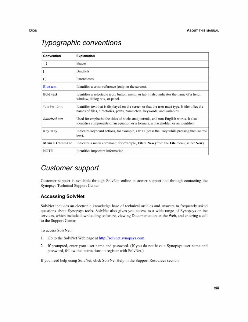
Typographic conventions
Customer supportCustomer support is available through SolvNet online customer support and through contacting theSynopsys Technical Support Center.
Accessing SolvNet
SolvNet includes an electronic knowledge base of technical articles and answers to frequently askedquestions about Synopsys tools. SolvNet also gives you access to a wide range of Synopsys onlineservices, which include downloading software, viewing Documentation on the Web, and entering a callto the Support Center.
To access SolvNet:
1. Go to the SolvNet Web page at http://solvnet.synopsys.com.
2. If prompted, enter your user name and password. (If you do not have a Synopsys user name andpassword, follow the instructions to register with SolvNet.)
If you need help using SolvNet, click SolvNet Help in the Support Resources section.
Convention Explanation
{ } Braces
[ ] Brackets
( ) Parentheses
Blue text Identifies a cross-reference (only on the screen).
Bold text Identifies a selectable icon, button, menu, or tab. It also indicates the name of a field, window, dialog box, or panel.
Courier font Identifies text that is displayed on the screen or that the user must type. It identifies the names of files, directories, paths, parameters, keywords, and variables.
Italicized text Used for emphasis, the titles of books and journals, and non-English words. It also identifies components of an equation or a formula, a placeholder, or an identifier.
Key+Key Indicates keyboard actions, for example, Ctrl+I (press the I key while pressing the Control key).
Menu > Command Indicates a menu command, for example, File > New (from the File menu, select New).
NOTE Identifies important information.
xiii

DIOSABOUT THIS MANUAL
Contacting the Synopsys Technical Support Center
If you have problems, questions, or suggestions, you can contact the Synopsys Technical Support Centerin the following ways:
Open a call to your local support center from the Web by going to http://solvnet.synopsys.com(Synopsys user name and password required), then clicking “Enter a Call to the Support Center.”
Send an e-mail message to your local support center:
• E-mail [email protected] from within North America.
• Find other local support center e-mail addresses at http://www.synopsys.com/support/support_ctr.
Telephone your local support center:
• Call (800) 245-8005 from within the continental United States.
• Call (650) 584-4200 from Canada.
• Find other local support center telephone numbers at http://www.synopsys.com/support/support_ctr.
Contacting your local TCAD Support Team directly
Send an e-mail message to:
[email protected] from within North America and South America.
[email protected] from within Europe.
[email protected] from within Asia Pacific (China, Taiwan, Singapore, Malaysia,India, Australia).
[email protected] from Korea.
[email protected] from Japan.
xiv
DIOS CHAPTER 1 GETTING STARTED
Dios
CHAPTER 1 Getting started
1.1 About DiosDios takes as its input a sequence of commands, which can be entered from standard input (that is, at theprompt in a command window) or composed in a command file. An optional additional input is a Prolytmask file containing details of geometries for the various mask levels. The simulation of a process flowis achieved by issuing a sequence of commands corresponding to the individual process steps. Inaddition, a number of control commands are provided to allow users to select physical models andparameters, grid strategies, and graphical output preferences if required.
1.1.1 Starting Dios
Dios is used interactively. A whole process flow can be simulated by entering commands line-by-line asstandard input. For interactive use, Dios is started by typing the command dios in a command window:
> dios
At start-up, details such as the time, date, version, and specifications of the host machine are given inthe standard output. Dios commands can be entered at the prompt:
dios>
This is a flexible way of working with Dios to test individual process steps or short sequences, but it isinconvenient for long process flows. Generally, it is more suitable to compile the command sequenceinto a command file, which can be run in batch mode or in Sentaurus Workbench.
1.1.2 Starting different versions of Dios
A particular release and version number of Dios can be selected using the -rel and -ver options:
dios -rel <rel_number> -ver <version_number>
For example:
dios -rel 9.5dios -ver 9.5.6
The command:
dios -rel 9.5 -ver 9.5.6
commences the simulation of the process ‘nmos’ using version 9.5.6 of Release 9.5 as long as thisversion is installed.
1
DIOSCHAPTER 1 GETTING STARTED
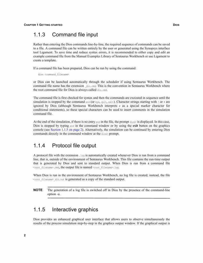
1.1.3 Command file input
Rather than entering the Dios commands line-by-line, the required sequence of commands can be savedto a file. A command file can be written entirely by the user or generated using the Synopsys interfacetool Ligament. To save time and reduce syntax errors, it is recommended to either copy and edit anexample command file from the Manual Examples Library of Sentaurus Workbench or use Ligament tocreate a template.
If a command file has been prepared, Dios can be run by using the command:
dios <command_filename>
or Dios can be launched automatically through the scheduler if using Sentaurus Workbench. Thecommand file name has the extension _dio.cmd. This is the convention in Sentaurus Workbench wherethe root command file for Dios is always called dio.cmd.
The command file is first checked for syntax and then the commands are executed in sequence until thesimulation is stopped by the command end (or bye, quit, exit). Character strings starting with ! or # areignored by Dios (although Sentaurus Workbench interprets # as a special marker character forconditional statements), so these special characters can be used to insert comments in the simulationcommand file.
At the end of the simulation, if there is no entry end in the file, the prompt dios> is displayed. In this case,Dios is stopped by typing end in the command window or by using the exit button on the graphicsconsole (see Section 1.1.5 on page 2). Alternatively, the simulation can be continued by entering Dioscommands directly in the command window at the dios> prompt.
1.1.4 Protocol file output
A protocol file with the extension .log is automatically created whenever Dios is run from a commandline, that is, outside of the environment of Sentaurus Workbench. This file contains the run-time outputthat is generated by Dios and sent to standard output. When Dios is run from a command file<root_filename>.cmd, the output file is named <root_filename>.log.
When Dios is run in the environment of Sentaurus Workbench, no log file is created; instead, the file<root_filename>_dio.out is generated as a copy of the standard output.
NOTE The generation of a log file is switched off in Dios by the presence of the command-lineoption -u.
1.1.5 Interactive graphics
Dios provides an enhanced graphical user interface that allows users to observe simultaneously theresults of the process simulation step-by-step in the graphics output window. If the graphical output is
2
DIOS CHAPTER 1 GETTING STARTED
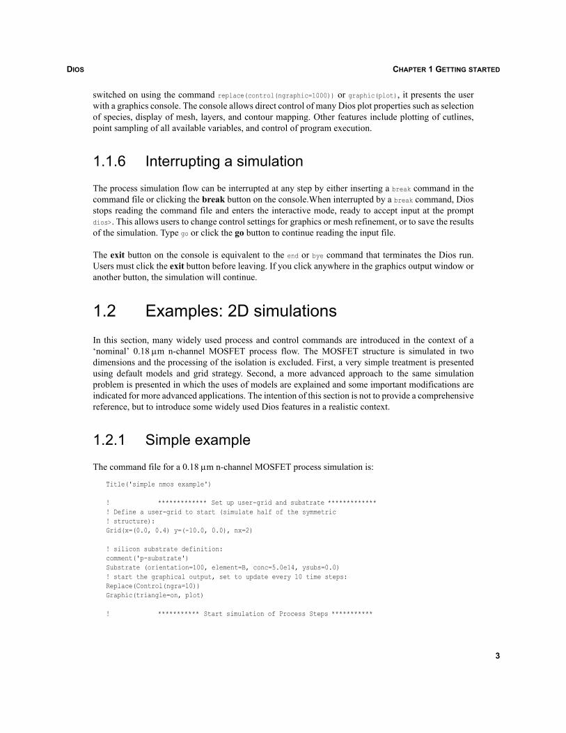
switched on using the command replace(control(ngraphic=1000)) or graphic(plot), it presents the userwith a graphics console. The console allows direct control of many Dios plot properties such as selectionof species, display of mesh, layers, and contour mapping. Other features include plotting of cutlines,point sampling of all available variables, and control of program execution.
1.1.6 Interrupting a simulation
The process simulation flow can be interrupted at any step by either inserting a break command in thecommand file or clicking the break button on the console.When interrupted by a break command, Diosstops reading the command file and enters the interactive mode, ready to accept input at the promptdios>. This allows users to change control settings for graphics or mesh refinement, or to save the resultsof the simulation. Type go or click the go button to continue reading the input file.
The exit button on the console is equivalent to the end or bye command that terminates the Dios run.Users must click the exit button before leaving. If you click anywhere in the graphics output window oranother button, the simulation will continue.
1.2 Examples: 2D simulationsIn this section, many widely used process and control commands are introduced in the context of a‘nominal’ 0.18 μm n-channel MOSFET process flow. The MOSFET structure is simulated in twodimensions and the processing of the isolation is excluded. First, a very simple treatment is presentedusing default models and grid strategy. Second, a more advanced approach to the same simulationproblem is presented in which the uses of models are explained and some important modifications areindicated for more advanced applications. The intention of this section is not to provide a comprehensivereference, but to introduce some widely used Dios features in a realistic context.
1.2.1 Simple example
The command file for a 0.18 μm n-channel MOSFET process simulation is:
Title('simple nmos example')
! ************* Set up user-grid and substrate *************! Define a user-grid to start (simulate half of the symmetric! structure):Grid(x=(0.0, 0.4) y=(-10.0, 0.0), nx=2)
! silicon substrate definition:comment('p-substrate')Substrate (orientation=100, element=B, conc=5.0e14, ysubs=0.0)! start the graphical output, set to update every 10 time steps:Replace(Control(ngra=10))Graphic(triangle=on, plot)
! *********** Start simulation of Process Steps ***********
3
DIOSCHAPTER 1 GETTING STARTED
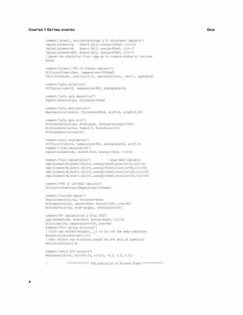
comment('p-well, anti-punchthrough & Vt adjustment implants')Implant(element=B, dose=2.0e13, energy=300keV, tilt=0)Implant(element=B, dose=1.0e13, energy=80keV, tilt=7)Implant(element=BF2, dose=2.0e12, energy=25keV, tilt=7)! pause the simulation flow: type go in command window to continuebreak
comment('p-well: RTA of channel implants')Diffusion(time=10sec, temperature=1050degC)1d(file=channel, xsection(0.0), species(btotal), fac=-1, append=on)
comment('gate oxidation')Diffusion(time=10, temperature=900, atmosphere=O2)
comment('poly gate deposition')Deposit(material=po, thickness=180nm)
comment('poly gate pattern')Mask(material=resist, thickness=800nm, xleft=0, xright=0.09)
comment('poly gate etch')Etching(material=po, stop=oxgas, rate(anisotropic=100))Etching(material=ox, Time=0.5, Rate(Aniso=10))Etching(material=resist)
comment('poly reoxidation')diffusion(time=20, temperature=900, atmosphere=O2, po2=0.5)comment(’nldd implantation’)implant(element=As, dose=4.0E14, energy=10keV, tilt=0)
comment('halo implantation') ! Quad HALO implants:Impl(element=B,dose=1.0e13/4.,energy=20keV,rotation=0,tilt=30)Impl(element=B,dose=1.0e13/4.,energy=20keV,rotation=90,tilt=30)Impl(element=B,dose=1.0e13/4.,energy=20keV,rotation=180,tilt=30)Impl(element=B,dose=1.0e13/4.,energy=20keV,rotation=270,tilt=30)
comment('RTA of LDD/HALO implants')Diffusion(Time=5sec,TEmperature=1050degC)
comment('nitride spacer')Deposit(material=ni, thickness=60nm)Etch(material=ni, remove=60nm, rate(a1=100), over=40)Etch(material=ox, stop=(pogas), rate(aniso=100))
comment('N+ implantation & final RTA')Impl(element=As, dose=5e15, energy=40keV, tilt=0)Diff(time=10s, temperature=1050, atmo=N2) comment('full device structure')! first use reflect(window(...)) to cut off the deep substrate:Reflect(window(bottom=-1.0))! then reflect the structure around the x=0 axis of symmetry:Reflect(reflect=0.0)
comment('metal S/D contacts')Mask(material=al, thick=0.03, x(-0.5, -0.2, 0.2, 0.5))
! ************* End simulation of Process Steps *************
4
DIOS CHAPTER 1 GETTING STARTED
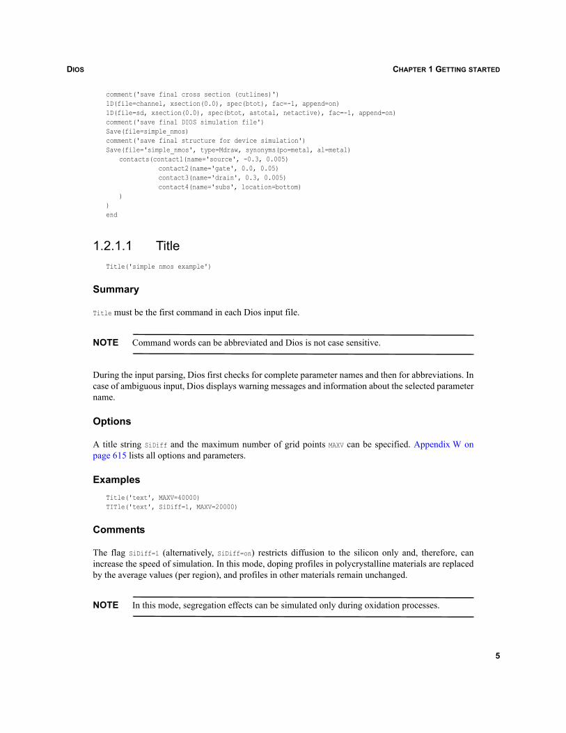
comment('save final cross section (cutlines)')1D(file=channel, xsection(0.0), spec(btot), fac=-1, append=on)1D(file=sd, xsection(0.0), spec(btot, astotal, netactive), fac=-1, append=on)comment('save final DIOS simulation file')Save(file=simple_nmos)comment('save final structure for device simulation')Save(file='simple_nmos', type=Mdraw, synonyms(po=metal, al=metal)
contacts(contact1(name='source', -0.3, 0.005)contact2(name='gate', 0.0, 0.05)contact3(name='drain', 0.3, 0.005)contact4(name='subs', location=bottom)
))end
1.2.1.1 TitleTitle('simple nmos example')
Summary
Title must be the first command in each Dios input file.
NOTE Command words can be abbreviated and Dios is not case sensitive.
During the input parsing, Dios first checks for complete parameter names and then for abbreviations. Incase of ambiguous input, Dios displays warning messages and information about the selected parametername.
Options
A title string SiDiff and the maximum number of grid points MAXV can be specified. Appendix W onpage 615 lists all options and parameters.
ExamplesTitle('text', MAXV=40000)TITle('text', SiDiff=1, MAXV=20000)
Comments
The flag SiDiff=1 (alternatively, SiDiff=on) restricts diffusion to the silicon only and, therefore, canincrease the speed of simulation. In this mode, doping profiles in polycrystalline materials are replacedby the average values (per region), and profiles in other materials remain unchanged.
NOTE In this mode, segregation effects can be simulated only during oxidation processes.
5
DIOSCHAPTER 1 GETTING STARTED
If it is important to include segregation effects in inert steps or to include diffusion in overlayers,SiDiff=0 (alternatively, SiDiff=off) must be specified. If SiDiff is not specified, SiDiff=1 is assumed bydefault.
MAXV sets a limit to the number of vertices (nodes) that can be generated by adaptive meshing. It isgenerally recommended to use this parameter to restrict mesh proliferation in cases where the meshingcriteria have not been carefully considered.
1.2.1.2 GridGrid(x=(0.0, 0.4) y=(-10.0, 0.0), nx=2)
Summary
After the Title command, an initial grid (or user grid) can be defined using the Grid command. Arectangular domain defined by the x-y coordinates is tessellated using nearly equilateral triangles. TheGrid command can be used repeatedly during a simulation to define a different user grid if required.
NOTE Dios uses a right-handed coordinate system. The x-axis points laterally to the right and the y-axis points vertically to the top. The y-axis is always perpendicular to the wafer surface.
Options
Initial triangle spacing is defined by either dx or nx. In the above case of nx=2, the user-defined startingmesh has the domain divided into two triangles with bases of 0.2 μm aligned along the x-axis.
Alternatively, the smallest possible side of an equilateral triangle can be defined explicitly using dx,which then determines nx indirectly. The relationship between nx and dx is explained in Section 1.2.2.3on page 25.
Examplesgrid(x=(-3,3),y=(1,-2.5),dx=50nm)
1.2.1.3 CommentComment('p-substrate')
Summary
Comment allows a text string to become the new (sub)title, typically at the start of a new process module.This string is adopted as the title in the Dios graphic and is included in the dataset labels of any 1Dprofiles saved while it is current.
6
DIOS CHAPTER 1 GETTING STARTED
1.2.1.4 SubstrateSUBStrate(ORIentation=100, ELEMent=B, CONCentration=5.0e14, ysubs=0.0)
Summary
After defining a user grid, the extent and the properties of the substrate layer must be defined.
Options
ELEMent The dopant species with which the substrate is doped.
CONCentration The uniform background doping concentration in the substrate [cm–3].Alternatively, the resistivity of the wafer [Ω cm] can be prescribed (RHO). IfCONCentration 0 and no resistivity is specified, no background doping isassumed.
ysubs The y-location of the top of the substrate (0.0 by default).
ORIentation The crystal orientation of the substrate surface: 110, 111, or 100 (default).
NOTE Oxidation rates are orientation dependent.
1.2.1.5 ControlReplace(Control(NGRAphic=10))
Summary
The parameter record Control is used for general Dios control purposes, in particular, for controlling gridadaptation and run-time output. The default Control parameters in the parameter record can be modifiedusing the Replace command at any point after the Title command.
In this case, the Dios graphics mode is initiated. The image is updated after each ten time steps ofdiffusion, deposition, and etching, and at the end of every processing step.
≤
7
DIOSCHAPTER 1 GETTING STARTED
Options
The modified Control parameters can be restricted to a specific process step by including the Controldefinition inside the process step itself. For example:
DIFFusion(Time=10sec, Temperature=1050, Control(LPRot=2))
increases the amount of information regarding this diffusion step, which is printed to the protocol file.
1.2.1.6 GraphicGraphic(Triangle=on, Plot)
Summary
The Graphic command starts and controls the Dios graphics output. If there is no Graphic command, butReplace(Control(NGRA=1000), the Dios graphics start automatically after the first process step is completed.The appearance of the Dios graphical output can be controlled from the command line or console.
NOTE More commands are available in the command line than appear on the console.
Options
SPEcies Selects the species to display (or click the species button and select an option).
Triangle=On/Off Toggles the display of the Dios mesh (or click the triangle button).
Equal=On/Off Toggles the equal scaling of the axes (or click the =/!= button).
SCale(XL,XR,YB,YT) Specifies view window (or zoom with left mouse button).
Zscale Allows the values in the legend for 2D isoline plots to be defined as a list.
Plot Forces the graphic to be replotted. Without the Plot specifier (or the Crossspecifier for 1D cross sections), Graphic has no effect.
In the graphics window
Zoom Drag the pointer to define the zoom window.
Recenter Click to define the new center for the plot.
Cutline A cutline is generated using the center mouse button. Drag the pointer to definethe cutline. When in cutline mode, the species can be reselected. Return to the2D plot by right-clicking in the plot window.
Sample After switching mode, click the move/sample button to see the concentrationvalues of the actual species. The values are printed to standard output with otheralphanumeric output.
8
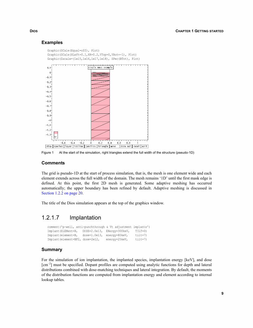
DIOS CHAPTER 1 GETTING STARTED
ExamplesGraphic(SCale(Equal=off), Plot)Graphic(SCale(XLeft=0.1,XR=0.2,YTop=0,YBot=-1), Plot)Graphic(Zscale=(1e15,1e16,1e17,1e18), SPec(BTot), Plot)
Figure 1 At the start of the simulation, right triangles extend the full width of the structure (pseudo-1D)
Comments
The grid is pseudo-1D at the start of process simulation, that is, the mesh is one element wide and eachelement extends across the full width of the domain. The mesh remains ‘1D’ until the first mask edge isdefined. At this point, the first 2D mesh is generated. Some adaptive meshing has occurredautomatically; the upper boundary has been refined by default. Adaptive meshing is discussed inSection 1.2.2 on page 20.
The title of the Dios simulation appears at the top of the graphics window.
1.2.1.7 Implantationcomment('p-well, anti-punchthrough & Vt adjustment implants')Implant(ELEMent=B, DOSE=2.0e13, ENergy=300keV, TILT=0)Implant(element=B, dose=1.0e13, energy=80keV, tilt=7)Implant(element=BF2, dose=2e12, energy=25keV, tilt=7)
Summary
For the simulation of ion implantation, the implanted species, implantation energy [keV], and dose[cm–2] must be specified. Dopant profiles are computed using analytic functions for depth and lateraldistributions combined with dose-matching techniques and lateral integration. By default, the momentsof the distribution functions are computed from implantation energy and element according to internallookup tables.
9
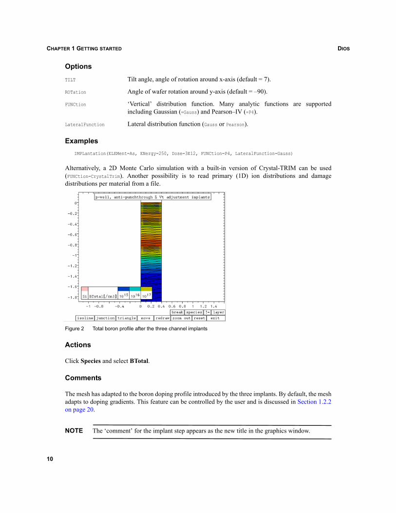
DIOSCHAPTER 1 GETTING STARTED
Options
TILT Tilt angle, angle of rotation around x-axis (default = 7).
ROTation Angle of wafer rotation around y-axis (default = –90).
FUNCtion ‘Vertical’ distribution function. Many analytic functions are supportedincluding Gaussian (=Gauss) and Pearson–IV (=P4).
LateralFunction Lateral distribution function (Gauss or Pearson).
ExamplesIMPLantation(ELEMent=As, ENergy=250, Dose=3E12, FUNCtion=P4, LateralFunction=Gauss)
Alternatively, a 2D Monte Carlo simulation with a built-in version of Crystal-TRIM can be used(FUNCtion=CrystalTrim). Another possibility is to read primary (1D) ion distributions and damagedistributions per material from a file.
Figure 2 Total boron profile after the three channel implants
Actions
Click Species and select BTotal.
Comments
The mesh has adapted to the boron doping profile introduced by the three implants. By default, the meshadapts to doping gradients. This feature can be controlled by the user and is discussed in Section 1.2.2on page 20.
NOTE The ‘comment’ for the implant step appears as the new title in the graphics window.
10
DIOS CHAPTER 1 GETTING STARTED
1.2.1.8 DiffusionComment('p-well: RTA of channel implants')DIFFusion(time=10sec, temperature=1050degC)
Summary
All high-temperature processes are controlled by the Diffusion command: RTA, predepositions, furnaceanneals, oxidation, epitaxy, and prebakes.
Temperature [oC] must be specified with either processing time (default unit is minute), or finalthickness [μm] in the case of oxidation, or growth rate [nm/minute] and time [minute], or thickness inthe case of epitaxy.
Options
TempRate Defines a temperature ramp rate between two values [K/minute].
ModDiff Selects the diffusion model (see Section 1.2.2 on page 20).
ExamplesDIFF(Time=(2s,5s,3s), TEmperature=(800,1050,1050,800))DIFF(Temperature=(800,1050), TempRate=10)
1.2.1.9 OxidationComment('gate oxidation')Diffusion(time=10, temperature=900, Atmosphere=O2)
Summary
Oxidation steps are implemented using the Diffusion command. Temperature and either processing timeor final thickness must be specified.
Default oxidation models are MODOx=Massoud and O2diffusion=Diffusion. The diffusion of the oxidantspecies in the oxide and its reaction at the silicon interface are computed.
Options
ATMOsphere Process ambient. One of H2O, O2, HCl, H2O2 (default inert: N2).
ExamplesDIFF(ATMOsphere=h2o, Temperature=1000, Time=100)DIFF(Temperature=1000, Time=100, Flow(O2=10l/min, HCl=0.3l/min))
11
DIOSCHAPTER 1 GETTING STARTED
1.2.1.10 Depositcomment('poly gate deposition')DEPOsit(Material=po, Thickness=180nm)
Summary
To simulate deposition processes, material and layer thicknesses are required. Alternatively, time[minute] and deposition rate (GrowthRate) [nm/minute] can be specified. The default model is LPCVD,which implies ‘isotropic’ deposition (see Section 7.2 on page 111).
Options
CONCentration Specifies the doping level of a deposited layer.
ELEMent Specifies the dopant species for a doped layer.
DTYPe Selects deposition model, for example, Anisotropic, Vertical, Fill.
See Appendix F on page 347 for a full listing and description.
ExamplesDEPO(MATer=PO, Time=1.8min, GrowthRate=100nm/min)DEPO(MATerial=PO, ELEM=P, CONC=3e19, THick=0.18)
1.2.1.11 Maskcomment('poly gate pattern')Mask(Material=resist, Thickness=800nm, xleft=0, xright=0.09)
Summary
Lithography simulation is replaced in Dios by the definition of resist masks. A single mask can bedefined by its left or right edge. If the mask extends over the left or right side of the simulation domain,the mask edge outside of the device can be specified, although this is not necessary (leave it undefined).It is not recommended to specify the left and right end of the simulation domain, since this may lead toround-off errors.
Options
See Section 1.2.2.15 on page 41 for a complete list.
ExamplesMASK(MATerial=PO, ELEM=P, CONC=3e19, THick=180nm, XLeft=0.2, XRight=0.4)Mask(Material=Resist,THick=2um, X=(0.2,0.4))
12
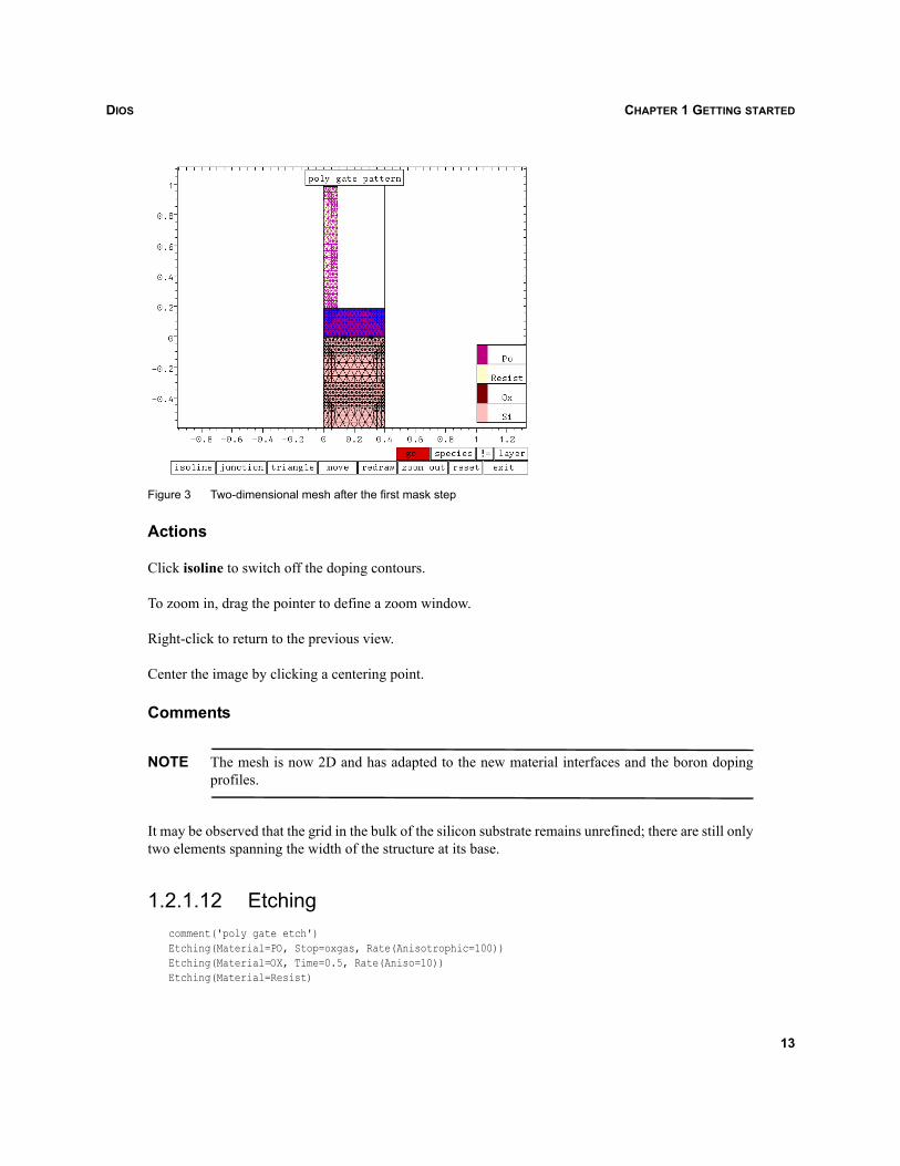
DIOS CHAPTER 1 GETTING STARTED
Figure 3 Two-dimensional mesh after the first mask step
Actions
Click isoline to switch off the doping contours.
To zoom in, drag the pointer to define a zoom window.
Right-click to return to the previous view.
Center the image by clicking a centering point.
Comments
NOTE The mesh is now 2D and has adapted to the new material interfaces and the boron dopingprofiles.
It may be observed that the grid in the bulk of the silicon substrate remains unrefined; there are still onlytwo elements spanning the width of the structure at its base.
1.2.1.12 Etchingcomment('poly gate etch')Etching(Material=PO, Stop=oxgas, Rate(Anisotrophic=100))Etching(Material=OX, Time=0.5, Rate(Aniso=10))Etching(Material=Resist)
13
DIOSCHAPTER 1 GETTING STARTED
Summary
Both the polysilicon gate and gate oxide are etched anisotropically.
Etch simulation in Dios is essentially geometric. Different degrees of anisotropy can be defined. In thiscase, perfectly anisotropic (perpendicular) etching of the polysilicon and oxide layers is specified at ratesof 100 nm/minute and 10 nm/minute, respectively.
A perfect etch stop at the oxide surface is assumed for the poly etch; the etch stops whenever theoxide–gas interface is exposed (Stop=oxgas). Similarly, the oxide etch stops at the silicon surface.
In addition, etch selectivity is assumed to be infinite. Different degrees of etch selectivity can optionallybe defined.
The command Etching(Material=Resist) removes the resist strip. All layers of resist that are in contactwith the gas are removed completely. Any other layers on top of or inside the resist are also removed.
Options
The etch depth for a certain material can be defined by a combination of Rate and Time. The Rate can bea combination of anisotropic (A1) and isotropic (Iso) contributions.
Remove=<etch depth in mm> Emulates a perfectly isotropic etch process such as a wet etch.
Over Defines an overetch in percentage, whether the etch be defined by rate and time,etch stop, or depth (remove).
NOTE An overetch of 10% is performed by default.
ExamplesEtching(MATerial=PO, Time=4, Rate(A1=300, Iso=100))ETCH(material=ox, REmove=0.006um)
1.2.1.13 Polysilicon reoxidationcomment('poly reoxidation')Diffusion(Time=20, Temperature=900, Atmosphere=O2, PO2=0.5)
Summary
The polysilicon gate is reoxidized in a dry oxygen ambient with an O2 partial pressure of 0.5 atm. Thedefault oxidation models are:
O2Diffusion=DiffusionMODOx=MassoudMECHanics(Solver=Uzawa)Stress dependency: off
14
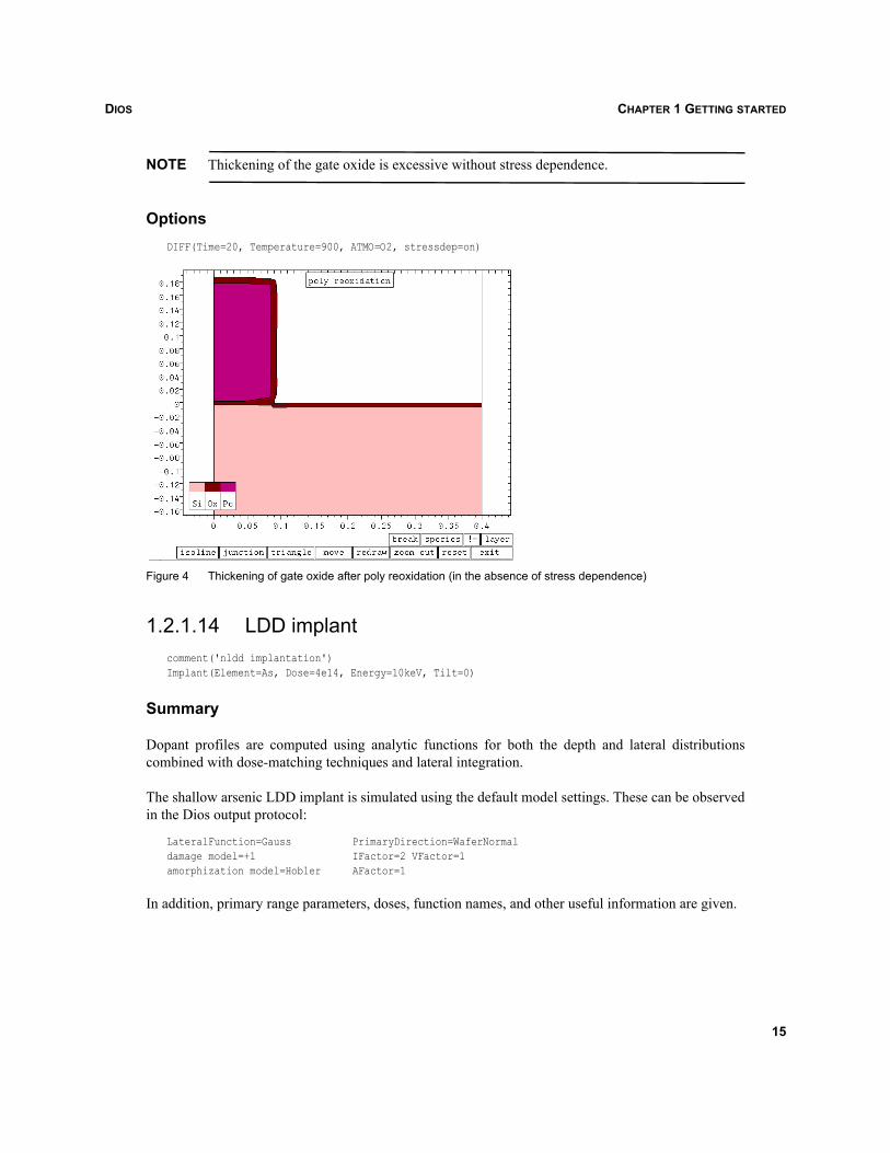
DIOS CHAPTER 1 GETTING STARTED
NOTE Thickening of the gate oxide is excessive without stress dependence.
OptionsDIFF(Time=20, Temperature=900, ATMO=O2, stressdep=on)
Figure 4 Thickening of gate oxide after poly reoxidation (in the absence of stress dependence)
1.2.1.14 LDD implantcomment('nldd implantation')Implant(Element=As, Dose=4e14, Energy=10keV, Tilt=0)
Summary
Dopant profiles are computed using analytic functions for both the depth and lateral distributionscombined with dose-matching techniques and lateral integration.
The shallow arsenic LDD implant is simulated using the default model settings. These can be observedin the Dios output protocol:
LateralFunction=Gauss PrimaryDirection=WaferNormaldamage model=+1 IFactor=2 VFactor=1amorphization model=Hobler AFactor=1
In addition, primary range parameters, doses, function names, and other useful information are given.
15

DIOSCHAPTER 1 GETTING STARTED
Comments
The default damage model is +1, which implies that one excess interstitial is generated for eachimplanted ion (IFactor-VFactor=1). At the same time, the amorphization of the silicon is being simulatedusing the Hobler model.
Figure 5 Plot of the damage profile used to evaluate amorphization
1.2.1.15 Halo implantscomment('halo implantation')Impl(ELEM=B,Dose=1e13/4.,EN=20keV,ROTat=0,Tilt=30)Impl(ELEM=B,Dose=1e13/4.,EN=20keV,ROTat=90,Tilt=30)Impl(ELEM=B,Dose=1e13/4.,EN=20keV,ROTat=180,Tilt=30)Impl(ELEM=B,Dose=1e13/4.,EN=20keV,ROTat=270,Tilt=30)
Summary
The tilted quad boron halo implants are performed in sequence. A quad implant is assumed in which thewafer is rotated 90o for each quarter of the dose.
Comments
By default, DoseAccumulation=on. Therefore, the implant damage continues to be accumulated and thevolume of amorphized silicon increases. The interstitial concentration can be viewed by selectingSpecies and ITotal The amorphization can be viewed by selecting Species and Amorphization.Amorphization of the silicon occurs in the zone where ‘amorphization’ exceeds the threshold value of
cm–3.1.15 1022×
16
DIOS CHAPTER 1 GETTING STARTED
Options
The four single-step implantations can be replaced by a single command:
Impl(ELEM=B,Dose=1e13,EN=20,Tilt=30,NumSplits=4)
Here, a sequence of implantations is simulated, each with the rotation angle increased by 360/NumSplitscompared to the previous. The dose for each of these steps equals Dose/NumSplits.
1.2.1.16 RTA of LDD/HALO implantsComment('RTA of LDD/HALO implants')Diffusion(Time=5sec,TEmperature=1050degC)
Summary
A simple diffusion step with no temperature ramps. The default diffusion model is (from the outputprotocol):
As Si ModDif: EquilibriumB Si ModDif: Equilibrium
Comments
In this example, the default condition SiDiff=on is active and diffusion is only computed in the silicon.The doping profile in the polysilicon is reduced to a constant level with the same dose for each region.
In addition, the default equilibrium diffusion model is used. Therefore, the point defects (vacancies andinterstitials) are replaced by their equilibrium concentrations.
In effect, the excess interstitials introduced by the LDD/HALO implant damage are assumed to haverecombined infinitely and quickly. In general, this is unrealistic. In the advanced example, morecomplete diffusion models, including point-defect coupling effects, are introduced.
Options
To retain the doping profile in the polysilicon and simulate the diffusion in this material and the oxide,select SiDiff=0 (SiDiff=off):
Replace(Control(SiDiff=off))
ExamplesDIFFusion(Time=5s,Temperature=1050, ModDiff=PairDiffusion)DIFFusion(Time=5s,Temperature=1050)
17
DIOSCHAPTER 1 GETTING STARTED
1.2.1.17 Nitride spacerComment('nitride spacer')Depo(MATerial=ni, Thickness=60nm)Etch(MAT=ni, remove=60nm, rate(a1=100), over=40)Etch(Material=ox, stop=(pogas), rate(aniso=100))
Summary
The default nitride deposition is modeled as ‘LPCVD’ (isotropic). The anisotropic nitride etch naturallyleaves a residual sidewall spacer.
NOTE The specification is for a 40% overetch (over=40). A 10% overetch is included by default. Theanisotropic oxide etch removes the screen oxide.
Comments
The combination of an isotropic deposition and anisotropic etch gives a reasonable ‘emulation’ of anitride sidewall. More sophisticated deposition and etch models are available in Dios for applicationswhere feature shape is important.
1.2.1.18 N+ source–drain implantation and final RTAcomment('N+ implantation & final RTA')Impl(element=As, dose=5e15, energy=40keV, tilt=0)Diff(time=10s, temperature=1050, atmo=N2)
Summary
The source–drain implantation is modeled with the default interstitial point defect and Hobleramorphization models. The anneal is simulated using the default equilibrium model (equilibriumconcentrations of vacancies and interstitials) and is non-oxidizing. Therefore, there is no point-defectdiffusion.
Comments
Damage (vacancy and interstitial point defects) is computed during the implantation step, but boronredistribution due to coupled point-defect diffusion is not simulated in the diffusion step. This isincluded in the advanced example.
1.2.1.19 Reflectcomment('full device structure')Reflect(window(bottom=-1.0))Reflect(reflect=0.0)
18
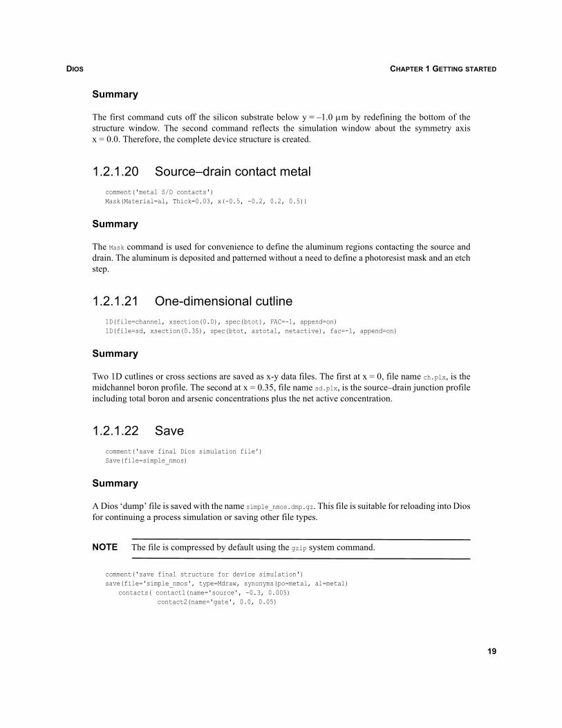
DIOS CHAPTER 1 GETTING STARTED
Summary
The first command cuts off the silicon substrate below y = –1.0 μm by redefining the bottom of thestructure window. The second command reflects the simulation window about the symmetry axisx = 0.0. Therefore, the complete device structure is created.
1.2.1.20 Source–drain contact metalcomment('metal S/D contacts')Mask(Material=al, Thick=0.03, x(-0.5, -0.2, 0.2, 0.5))
Summary
The Mask command is used for convenience to define the aluminum regions contacting the source anddrain. The aluminum is deposited and patterned without a need to define a photoresist mask and an etchstep.
1.2.1.21 One-dimensional cutline1D(file=channel, xsection(0.0), spec(btot), FAC=-1, append=on)1D(file=sd, xsection(0.35), spec(btot, astotal, netactive), fac=-1, append=on)
Summary
Two 1D cutlines or cross sections are saved as x-y data files. The first at x = 0, file name ch.plx, is themidchannel boron profile. The second at x = 0.35, file name sd.plx, is the source–drain junction profileincluding total boron and arsenic concentrations plus the net active concentration.
1.2.1.22 Savecomment('save final Dios simulation file')Save(file=simple_nmos)
Summary
A Dios ‘dump’ file is saved with the name simple_nmos.dmp.gz. This file is suitable for reloading into Diosfor continuing a process simulation or saving other file types.
NOTE The file is compressed by default using the gzip system command.
comment('save final structure for device simulation')save(file='simple_nmos', type=Mdraw, synonyms(po=metal, al=metal)
contacts( contact1(name='source', -0.3, 0.005)contact2(name='gate', 0.0, 0.05)
19
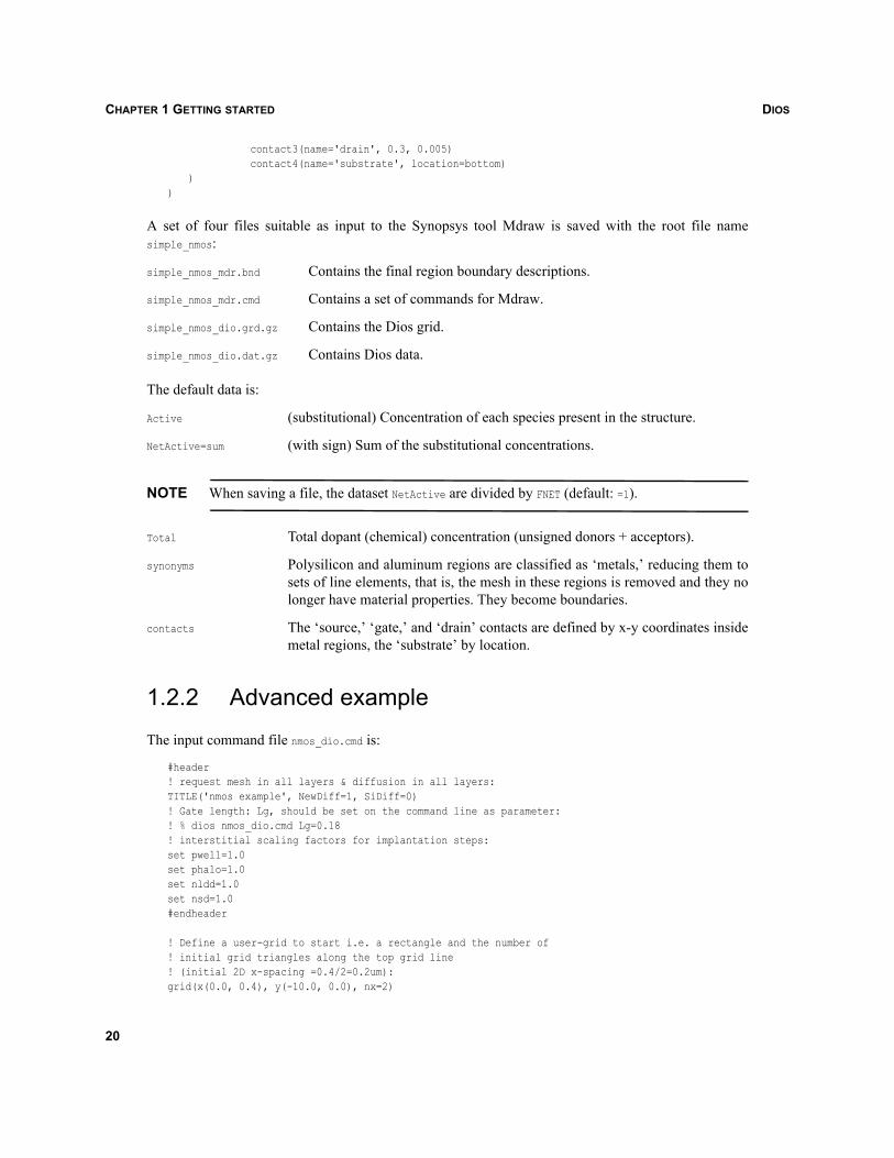
DIOSCHAPTER 1 GETTING STARTED
contact3(name='drain', 0.3, 0.005)contact4(name='substrate', location=bottom)
))
A set of four files suitable as input to the Synopsys tool Mdraw is saved with the root file namesimple_nmos:
simple_nmos_mdr.bnd Contains the final region boundary descriptions.
simple_nmos_mdr.cmd Contains a set of commands for Mdraw.
simple_nmos_dio.grd.gz Contains the Dios grid.
simple_nmos_dio.dat.gz Contains Dios data.
The default data is:
Active (substitutional) Concentration of each species present in the structure.
NetActive=sum (with sign) Sum of the substitutional concentrations.
NOTE When saving a file, the dataset NetActive are divided by FNET (default: =1).
Total Total dopant (chemical) concentration (unsigned donors + acceptors).
synonyms Polysilicon and aluminum regions are classified as ‘metals,’ reducing them tosets of line elements, that is, the mesh in these regions is removed and they nolonger have material properties. They become boundaries.
contacts The ‘source,’ ‘gate,’ and ‘drain’ contacts are defined by x-y coordinates insidemetal regions, the ‘substrate’ by location.
1.2.2 Advanced example
The input command file nmos_dio.cmd is:
#header! request mesh in all layers & diffusion in all layers: TITLE('nmos example', NewDiff=1, SiDiff=0)! Gate length: Lg, should be set on the command line as parameter:! % dios nmos_dio.cmd Lg=0.18! interstitial scaling factors for implantation steps:set pwell=1.0set phalo=1.0set nldd=1.0set nsd=1.0#endheader
! Define a user-grid to start i.e. a rectangle and the number of! initial grid triangles along the top grid line! (initial 2D x-spacing =0.4/2=0.2um):grid(x(0.0, 0.4), y(-10.0, 0.0), nx=2)
20
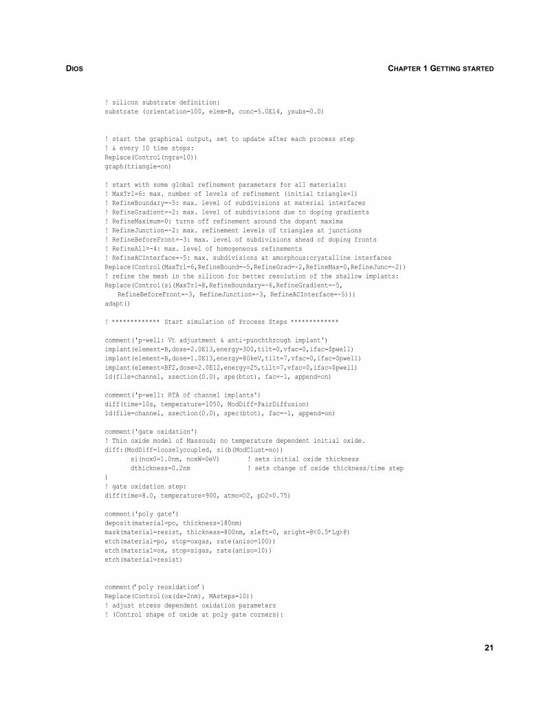
DIOS CHAPTER 1 GETTING STARTED
! silicon substrate definition:substrate (orientation=100, elem=B, conc=5.0E14, ysubs=0.0)
! start the graphical output, set to update after each process step! & every 10 time steps:Replace(Control(ngra=10))graph(triangle=on)
! start with some global refinement parameters for all materials:! MaxTrl=6: max. number of levels of refinement (initial triangle=1)! RefineBoundary=-5: max. level of subdivisions at material interfaces! RefineGradient=-2: max. level of subdivisions due to doping gradients! RefineMaximum=0: turns off refinement around the dopant maxima! RefineJunction=-2: max. refinement levels of triangles at junctions! RefineBeforeFront=-3: max. level of subdivisions ahead of doping fronts! RefineAll=-4: max. level of homogeneous refinements! RefineACInterface=-5: max. subdivisions at amorphous:crystalline interfacesReplace(Control(MaxTrl=6,RefineBound=-5,RefineGrad=-2,RefineMax=0,RefineJunc=-2))! refine the mesh in the silicon for better resolution of the shallow implants:Replace(Control(si(MaxTrl=8,RefineBoundary=-6,RefineGradient=-5,
RefineBeforeFront=-3, RefineJunction=-3, RefineACInterface=-5)))adapt()
! ************* Start simulation of Process Steps *************
comment('p-well: Vt adjustment & anti-punchthrough implant')implant(element=B,dose=2.0E13,energy=300,tilt=0,vfac=0,ifac=$pwell)implant(element=B,dose=1.0E13,energy=80keV,tilt=7,vfac=0,ifac=$pwell)implant(element=BF2,dose=2.0E12,energy=25,tilt=7,vfac=0,ifac=$pwell)1d(file=channel, xsection(0.0), spe(btot), fac=-1, append=on)
comment('p-well: RTA of channel implants')diff(time=10s, temperature=1050, ModDiff=PairDiffusion)1d(file=channel, xsection(0.0), spec(btot), fac=-1, append=on)
comment('gate oxidation')! Thin oxide model of Massoud; no temperature dependent initial oxide.diff:(ModDiff=looselycoupled, si(b(ModClust=no))
si(nox0=1.0nm, noxW=0eV) ! sets initial oxide thicknessdthickness=0.2nm ! sets change of oxide thickness/time step
)! gate oxidation step:diff(time=8.0, temperature=900, atmo=O2, pO2=0.75)
comment('poly gate')deposit(material=po, thickness=180nm)mask(material=resist, thickness=800nm, xleft=0, xright=@<0.5*Lg>@)etch(material=po, stop=oxgas, rate(aniso=100))etch(material=ox, stop=sigas, rate(aniso=10))etch(material=resist)
comment(’poly reoxidation’)Replace(Control(ox(dx=2nm), MAsteps=10))! adjust stress dependent oxidation parameters! (Control shape of oxide at poly gate corners):
21
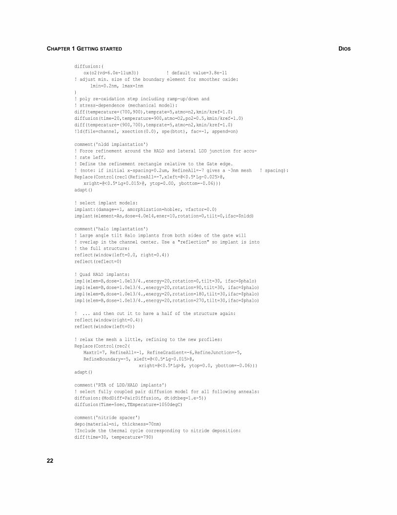
DIOSCHAPTER 1 GETTING STARTED
diffusion:(ox(o2(vd=6.0e-11um3)) ! default value=3.8e-11
! adjust min. size of the boundary element for smoother oxide: lmin=0.2nm, lmax=1nm)! poly re-oxidation step including ramp-up/down and! stress-dependence (mechanical model):diff(temperature=(700,900),temprate=5,atmo=n2,kmin/kref=1.0)diffusion(time=20,temperature=900,atmo=O2,po2=0.5,kmin/kref=1.0)diff(temperature=(900,700),temprate=5,atmo=n2,kmin/kref=1.0)!1d(file=channel, xsection(0.0), spe(btot), fac=-1, append=on)
comment('nldd implantation')! Force refinement around the HALO and lateral LDD junction for accu-! rate Leff.! Define the refinement rectangle relative to the Gate edge.! (note: if initial x-spacing=0.2um, RefineAll=-7 gives a ~3nm mesh ! spacing):Replace(Control(rec1(RefineAll=-7,xleft=@<0.5*Lg-0.025>@,
xright=@<0.5*Lg+0.015>@, ytop=0.00, ybottom=-0.06)))adapt()
! select implant models:implant:(damage=+1, amorphization=hobler, vfactor=0.0)implant(element=As,dose=4.0e14,ener=10,rotation=0,tilt=0,ifac=$nldd)
comment('halo implantation')! Large angle tilt Halo implants from both sides of the gate will! overlap in the channel center. Use a "reflection" so implant is into! the full structure:reflect(window(left=0.0, right=0.4))reflect(reflect=0)
! Quad HALO implants:impl(elem=B,dose=1.0e13/4.,energy=20,rotation=0,tilt=30, ifac=$phalo)impl(elem=B,dose=1.0e13/4.,energy=20,rotation=90,tilt=30, ifac=$phalo)impl(elem=B,dose=1.0e13/4.,energy=20,rotation=180,tilt=30,ifac=$phalo)impl(elem=B,dose=1.0e13/4.,energy=20,rotation=270,tilt=30,ifac=$phalo)
! ... and then cut it to have a half of the structure again:reflect(window(right=0.4))reflect(window(left=0))
! relax the mesh a little, refining to the new profiles:Replace(Control(rec2(
Maxtrl=7, RefineAll=-1, RefineGradient=-6,RefineJunction=-5,RefineBoundary=-5, xleft=@<0.5*Lg-0.015>@,
xright=@<0.5*Lg>@, ytop=0.0, ybottom=-0.06)))adapt()
comment('RTA of LDD/HALO implants')! select fully coupled pair diffusion model for all following anneals:diffusion:(ModDiff=PairDiffusion, dt(dtbeg=1.e-5))diffusion(Time=5sec,TEmperature=1050degC)
comment('nitride spacer')depo(material=ni, thickness=70nm)!Include the thermal cycle corresponding to nitride deposition:diff(time=30, temperature=790)
22
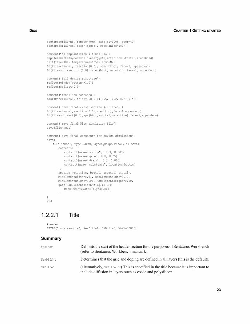
DIOS CHAPTER 1 GETTING STARTED
etch(material=ni, remove=70nm, rate(a1=100), over=40)etch(material=ox, stop=(pogas), rate(aniso=100))
comment(’N+ implantation & final RTA’)impl(element=As,dose=5e15,energy=40,rotation=0,tilt=0,ifac=$nsd)diff(time=10s, temperature=1050, atmo=N2)1d(file=channel, xsection(0.0), spec(btot), fac=-1, append=on)1d(file=sd, xsection(0.0), spec(btot, astotal’, fac=-1, append=on)
comment('full device structure')reflect(window(bottom=-1.0))reflect(reflect=0.0)
comment(’metal S/D contacts’)mask(material=al, thick=0.03, x(-0.5, -0.2, 0.2, 0.5))
comment('save final cross section (cutlines)')1d(file=channel,xsection(0.0),spe(btot),fac=-1,append=on)1d(file=sd,xsect(0.0),spe(btot,astotal,netactive),fac=-1,append=on)
comment('save final Dios simulation file')save(file=nmos)
comment('save final structure for device simulation')save(
file='nmos', type=Mdraw, synonyms(po=metal, al=metal)contacts(
contact1(name=’source’, -0.3, 0.005)contact2(name=’gate’, 0.0, 0.05)contact3(name=’drain’, 0.3, 0.005)contact4(name=’substrate’, location=bottom)
),species(netactive, btotal, astotal, ptotal),MinElementWidth=0.01, MaxElementWidth=0.10,MinElementHeight=0.01, MaxElementHeight=0.10,gate(MaxElementWidth=@<Lg/10.0>@
MinElementWidth=@<Lg/40.0>@)
)end
1.2.2.1 Title#headerTITLE('nmos example', NewDiff=1, SiDiff=0, MAXV=50000)
Summary
#header Delimits the start of the header section for the purposes of Sentaurus Workbench(refer to Sentaurus Workbench manual).
NewDiff=1 Determines that the grid and doping are defined in all layers (this is the default).
SiDiff=0 (alternatively, SiDiff=off) This is specified in the title because it is important toinclude diffusion in layers such as oxide and polysilicon.
23
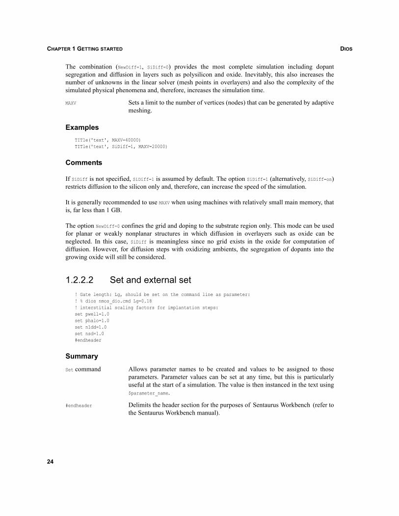
DIOSCHAPTER 1 GETTING STARTED
The combination (NewDiff=1, SiDiff=0) provides the most complete simulation including dopantsegregation and diffusion in layers such as polysilicon and oxide. Inevitably, this also increases thenumber of unknowns in the linear solver (mesh points in overlayers) and also the complexity of thesimulated physical phenomena and, therefore, increases the simulation time.
MAXV Sets a limit to the number of vertices (nodes) that can be generated by adaptivemeshing.
ExamplesTITle('text', MAXV=40000)TITle('text', SiDiff=1, MAXV=20000)
Comments
If SiDiff is not specified, SiDiff=1 is assumed by default. The option SiDiff=1 (alternatively, SiDiff=on)restricts diffusion to the silicon only and, therefore, can increase the speed of the simulation.
It is generally recommended to use MAXV when using machines with relatively small main memory, thatis, far less than 1 GB.
The option NewDiff=0 confines the grid and doping to the substrate region only. This mode can be usedfor planar or weakly nonplanar structures in which diffusion in overlayers such as oxide can beneglected. In this case, SiDiff is meaningless since no grid exists in the oxide for computation ofdiffusion. However, for diffusion steps with oxidizing ambients, the segregation of dopants into thegrowing oxide will still be considered.
1.2.2.2 Set and external set! Gate length: Lg, should be set on the command line as parameter:! % dios nmos_dio.cmd Lg=0.18! interstitial scaling factors for implantation steps:set pwell=1.0set phalo=1.0set nldd=1.0set nsd=1.0#endheader
Summary
Set command Allows parameter names to be created and values to be assigned to thoseparameters. Parameter values can be set at any time, but this is particularlyuseful at the start of a simulation. The value is then instanced in the text using$parameter_name.
#endheader Delimits the header section for the purposes of Sentaurus Workbench (refer tothe Sentaurus Workbench manual).
24
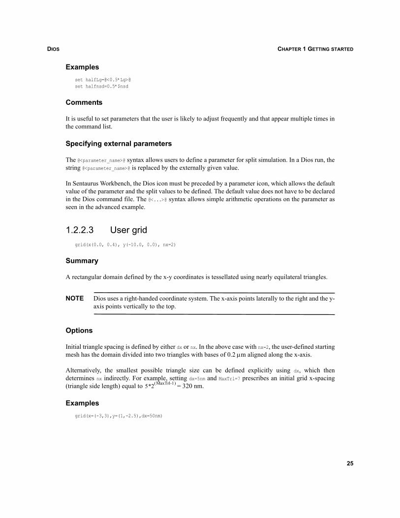
DIOS CHAPTER 1 GETTING STARTED
Examplesset halfLg=@<0.5*Lg>@set halfnsd=0.5*$nsd
Comments
It is useful to set parameters that the user is likely to adjust frequently and that appear multiple times inthe command list.
Specifying external parameters
The @<parameter_name>@ syntax allows users to define a parameter for split simulation. In a Dios run, thestring @<parameter_name>@ is replaced by the externally given value.
In Sentaurus Workbench, the Dios icon must be preceded by a parameter icon, which allows the defaultvalue of the parameter and the split values to be defined. The default value does not have to be declaredin the Dios command file. The @<...>@ syntax allows simple arithmetic operations on the parameter asseen in the advanced example.
1.2.2.3 User gridgrid(x(0.0, 0.4), y(-10.0, 0.0), nx=2)
Summary
A rectangular domain defined by the x-y coordinates is tessellated using nearly equilateral triangles.
NOTE Dios uses a right-handed coordinate system. The x-axis points laterally to the right and the y-axis points vertically to the top.
Options
Initial triangle spacing is defined by either dx or nx. In the above case with nx=2, the user-defined startingmesh has the domain divided into two triangles with bases of 0.2 μm aligned along the x-axis.
Alternatively, the smallest possible triangle size can be defined explicitly using dx, which thendetermines nx indirectly. For example, setting dx=5nm and MaxTrl=7 prescribes an initial grid x-spacing(triangle side length) equal to = 320 nm.
Examplesgrid(x=(-3,3),y=(1,-2.5),dx=50nm)
5*2 MaxTrl-1( )
25
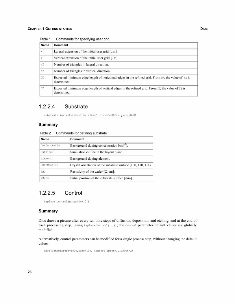
DIOSCHAPTER 1 GETTING STARTED
1.2.2.4 Substratesubstrate (orientation=100, elem=B, conc=5.0E14, ysubs=0.0)
Summary
1.2.2.5 ControlReplace(Control(ngraphic=10))
Summary
Dios draws a picture after every ten time steps of diffusion, deposition, and etching, and at the end ofeach processing step. Using Replace(Control(...)), the Control parameter default values are globallymodified.
Alternatively, control parameters can be modified for a single process step, without changing the defaultvalues:
diff(Temperature=1000,time=100, Control(lprot=2,IPRNwt=2))
Table 1 Commands for specifying user grid
Name Comment
X Lateral extension of the initial user grid [μm].
Y Vertical extension of the initial user grid [μm].
NX Number of triangles in lateral direction.
NY Number of triangles in vertical direction.
DX Expected minimum edge length of horizontal edges in the refined grid. From DX, the value of NX is determined.
DY Expected minimum edge length of vertical edges in the refined grid. From DY, the value of NY is determined.
Table 2 Commands for defining substrate
Name Comment
CONCentration Background doping concentration [cm–3].
Cutline() Simulation cutline in the layout plane.
ELEMent Background doping element.
ORIENtation Crystal orientation of the substrate surface (100, 110, 111).
RHO Resistivity of the wafer [Ω cm].
YSubs Initial position of the substrate surface [mm].
26
DIOS CHAPTER 1 GETTING STARTED
Options
Control(fullprotocol=on) Can be used to make a full printout of all parameters of a particularcommand.
This may result in a huge amount of output.
1.2.2.6 GraphicGraphic(Triangle=on, Plot)
Summary
The Graphic command starts and controls the Dios graphics output. By default, the layer system, the netprofile, and the p-n junctions are shown. The appearance of the Dios graphical output is controlled fromthe command line or by using the buttons on the console.
NOTE More commands are available in the command line than appear on the console.
For a detailed description of all graphical output parameters, see Chapter 13 on page 295.
Options
SPEcies Selects the species to display (alternatively, click the species button and selectan option).
Triangle=On/Off Switches the display of the Dios mesh (or click the triangle button).
Equal=On/Off Switches the equal scaling of the x-axis and y-axis.
SCale(XLeft XRight YBottom YTop=...)
Specifies the view window (or zoom with the left mouse button).
Zscale Allows the contour scale for 2D (x-y) plots to be defined as a list.
Plot Forces the graphic to be replotted.
XSection(...) Defines the location of vertical 1D cross sections. The command Cross
computes and draws the cross sections along the cutlines.
With the command gra(SUrface), 3D surface pictures of the selected species are drawn. By default, thefunctions are interpolated on a rectangular mesh. LIneplot allows external files containing 1D profiles tobe read and drawn.
In the graphics window
Zoom Drag the pointer to define the zoom window.
Recenter Click to define the new center for the plot.
27
DIOSCHAPTER 1 GETTING STARTED
Cutline A cutline is generated using the center mouse button. Drag the pointer to definethe cutline. When in cutline mode, the species can be reselected. Return to the2D plot by right-clicking in the window.
1.2.2.7 Grid adaptationReplace(Control(MaxTrl=6, RefineBoundary=-5, RefineGradient=-2, RefineMaximum=0, RefineJunc=-2))Replace(Control(si(MaxTrl=8, RefineBoundary=-6, RefineGradient=-5, RefineBeforeFront=5,
RefineJunction=-3, RefineACInterface=-5)))
Summary
The first command sets global refinement parameters for all materials. The maximum level of trianglerefinement (MaxTrl) in all layers is set to 6. The second command sets stronger refinement parameters forsilicon, providing a higher level of refinement in the silicon.
In Dios, the automatic adaptive meshing adjusts the mesh refinement according to the presence ofinterfaces and doping profiles in the device structure. This command defines a set of parameters for theautomatic grid adaptation as summarized in Table 3 on page 29 (see Appendix C on page 329).
MaxTrl defines the maximum level of refinement where level 1 corresponds to the initial user grid. In thisexample, the levels correspond to:
Level of refinement: 1 2 3 4 5 6 7
Triangle side length [μm]: 0.2 0.1 0.05 0.025 0.0125 0.00625 0.003125
NOTE If the parameters have negative values, the maximum level of refinement (MaxTrl) isrespected. However, if any refinement parameter is positive, this will disregard the MaxTrlsetting and lead to higher levels of refinement. Therefore, positive criteria should be specifiedcarefully.
Refinement criteria can be revised at any time in the simulation flow and can be defined for each materialgiving flexibility in grid control for more advanced users.
Examples
Refinement levels can be defined inside rectangular boxes ( boxes):
Replace(Control(REC1(MaxTrl=8,RefineBoundary=-7)
or inside specific materials:
Replace(Control(ox(MaxTrl=5,RefineBoundary=-5)
or the boundary can be refined at a specified material interface:
Replace(Control(siox(RefineBoundary=-8)))
10≤
28
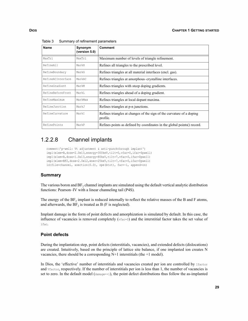
DIOS CHAPTER 1 GETTING STARTED
1.2.2.8 Channel implantscomment('p-well: Vt adjustment & anti-punchthrough implant')impl(elem=B,dose=2.0e13,energy=300keV,tilt=0,vfac=0,ifac=$pwell)impl(elem=B,dose=1.0e13,energy=80keV,tilt=7,vfac=0,ifac=$pwell)impl(elem=BF2,dose=2.0e12,ener=25keV,tilt=7,vfac=0,ifac=$pwell)1d(file=channel, xsection(0.0), spe(btot), fac=-1, append=on)
Summary
The various boron and BF2 channel implants are simulated using the default vertical analytic distributionfunctions: Pearson–IV with a linear channeling tail (P4S).
The energy of the BF2 implant is reduced internally to reflect the relative masses of the B and F atoms,and afterwards, the BF2 is treated as B (F is neglected).
Implant damage in the form of point defects and amorphization is simulated by default. In this case, theinfluence of vacancies is removed completely (vfac=0) and the interstitial factor takes the set value ofifac.
Point defects
During the implantation step, point defects (interstitials, vacancies), and extended defects (dislocations)are created. Intuitively, based on the principle of lattice site balance, if one implanted ion creates Nvacancies, there should be a corresponding N+1 interstitials (the +1 model).
In Dios, the ‘effective’ number of interstitials and vacancies created per ion are controlled by Ifactorand Vfactor, respectively. If the number of interstitials per ion is less than 1, the number of vacancies isset to zero. In the default model (damage=+1), the point defect distributions thus follow the as-implanted
Table 3 Summary of refinement parameters
Name Synonym (version 5.0)
Comment
MaxTrl MaxTrl Maximum number of levels of triangle refinement.
RefineAll MarkH Refines all triangles to the prescribed level.
RefineBoundary MarkG Refines triangles at all material interfaces (encl. gas).
RefineACInterface MarkAC Refines triangles at amorphous–crystalline interfaces.
RefineGradient MarkM Refines triangles with steep doping gradients.
RefineBeforeFront MarkL Refines triangles ahead of a doping gradient.
RefineMaximum MarkMax Refines triangles at local dopant maxima.
RefineJunction MarkJ Refines triangles at p-n junctions.
RefineCurvature MarkI Refines triangles at changes of the sign of the curvature of a doping profile.
RefinePoints MarkP Refines points as defined by coordinates in the global points() record.
29
DIOSCHAPTER 1 GETTING STARTED
profile. The alternative model is the Hobler function (damage=Hobler). The parameter damage can also betset to Monte Carlo damage (damage=MCdamage) when a Monte Carlo implantation is performed.
In the absence of any thermal step, the total damage accumulates for a sequence of implants. At the firstdiffusion statement following the implantation(s), all vacancies are assumed to recombine instantly withavailable interstitials, leaving only the excess interstitial population. If the silicon is amorphous after theimplantation, the excess interstitial and vacancies disappear in the recrystallized amorphous layer.
Amorphization
By default, the amorphization of the silicon is computed based on the Hobler function(amorphization=Hobler). Wherever the damage induced by implantation exceeds a threshold value( cm–3), the silicon is assumed to be amorphous. The alternative amorphization model isbased on the as-implanted profile (amorphization=+1).
An amorphous layer is presumed to recrystallize immediately at the beginning of the first diffusion stepfollowing the implantation. This assumption is justified by the high rate of recrystallization ofamorphous silicon, even at low temperature.
Options
FitAsImplantedDose=on/off
Selects to fit the integrated dose of as-implanted profiles to the prescribed dose(default=on).
By default, the moments of the distribution functions are computed from the implantation, energy, andelement according to internal lookup tables. The moments can also be specified explicitly for eachmaterial:
implantation(ELEMent=As,Dose=3e12,FUNCtion=PEarson,SI(RP=... STDV=... GAMma=... BETA=... LEXP=... STDVL=...),OX(...))
RP, STDV, LEXP, and STDVL are lengths [μm], and GAMma and BETA are real numbers. There are another two rangeparameters: STDVSec for the jointed half-Gaussian and LEXPOW for functions with a general exponential tail.
Dual analytic primary distribution functions can be specified in three ways:
implantation(..., Function=DualPearson)implantation(..., Function(JHG,JHGK))implantation(..., Si(Function=P4,Function2=P4K))
The specification of dual analytic primary ion distributions should be accompanied by a vector of totaldoses and a vector of channeling doses in silicon:
implantation(...,Si(TotalDoses(5e12,1e13,1e14,1e15,5e15),ChannelingDoses(5e12,1e13,5e13,8e13,1e14))
From these two vectors, the actual partial doses for both components of the primary ion distributionfunction are computed with regard to the given dose. The channeling dose is always associated with thesecond component of a dual primary ion distribution.
1.15 1022×
30
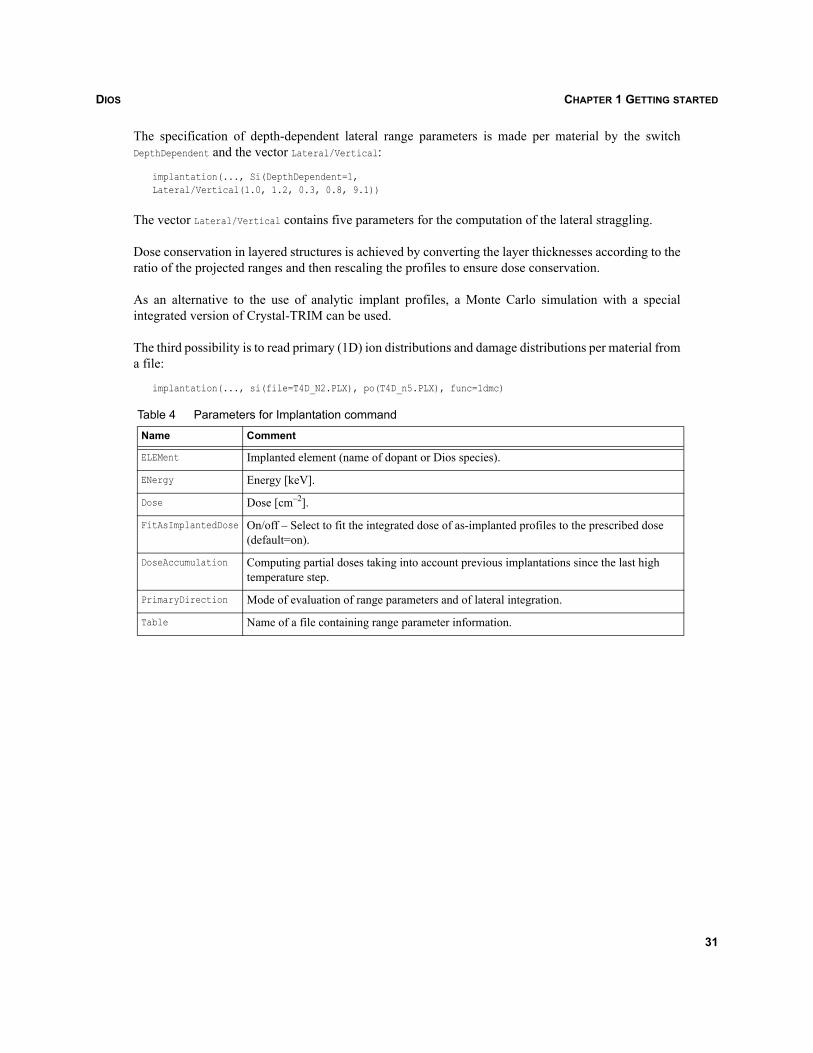
DIOS CHAPTER 1 GETTING STARTED
The specification of depth-dependent lateral range parameters is made per material by the switchDepthDependent and the vector Lateral/Vertical:
implantation(..., Si(DepthDependent=1,Lateral/Vertical(1.0, 1.2, 0.3, 0.8, 9.1))
The vector Lateral/Vertical contains five parameters for the computation of the lateral straggling.
Dose conservation in layered structures is achieved by converting the layer thicknesses according to theratio of the projected ranges and then rescaling the profiles to ensure dose conservation.
As an alternative to the use of analytic implant profiles, a Monte Carlo simulation with a specialintegrated version of Crystal-TRIM can be used.
The third possibility is to read primary (1D) ion distributions and damage distributions per material froma file:
implantation(..., si(file=T4D_N2.PLX), po(T4D_n5.PLX), func=1dmc)
Table 4 Parameters for Implantation command
Name Comment
ELEMent Implanted element (name of dopant or Dios species).
ENergy Energy [keV].
Dose Dose [cm–2].
FitAsImplantedDose On/off – Select to fit the integrated dose of as-implanted profiles to the prescribed dose (default=on).
DoseAccumulation Computing partial doses taking into account previous implantations since the last high temperature step.
PrimaryDirection Mode of evaluation of range parameters and of lateral integration.
Table Name of a file containing range parameter information.
31
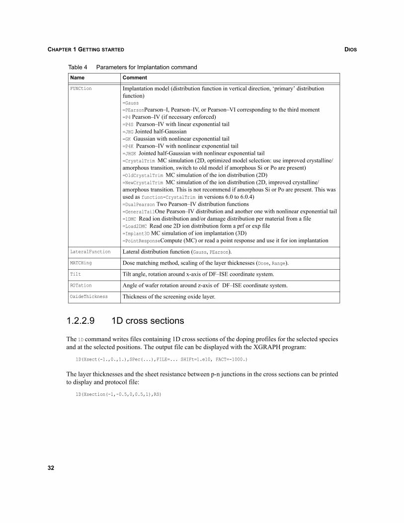
DIOSCHAPTER 1 GETTING STARTED
1.2.2.9 1D cross sections
The 1D command writes files containing 1D cross sections of the doping profiles for the selected speciesand at the selected positions. The output file can be displayed with the XGRAPH program:
1D(Xsect(-1.,0.,1.),SPec(...),FILE=... SHIFt=1.e10, FACT=-1000.)
The layer thicknesses and the sheet resistance between p-n junctions in the cross sections can be printedto display and protocol file:
1D(Xsection(-1,-0.5,0,0.5,1),RS)
FUNCtion Implantation model (distribution function in vertical direction, ‘primary’ distribution function) =Gauss=PEarsonPearson–I, Pearson–IV, or Pearson–VI corresponding to the third moment=P4 Pearson–IV (if necessary enforced)=P4S Pearson–IV with linear exponential tail=JHG Jointed half-Gaussian=GK Gaussian with nonlinear exponential tail=P4K Pearson–IV with nonlinear exponential tail=JHGK Jointed half-Gaussian with nonlinear exponential tail=CrystalTrim MC simulation (2D, optimized model selection: use improved crystalline/amorphous transition, switch to old model if amorphous Si or Po are present)=OldCrystalTrim MC simulation of the ion distribution (2D)=NewCrystalTrim MC simulation of the ion distribution (2D, improved crystalline/amorphous transition. This is not recommend if amorphous Si or Po are present. This was used as function=CrystalTrim in versions 6.0 to 6.0.4)=DualPearson Two Pearson–IV distribution functions=GeneralTailOne Pearson–IV distribution and another one with nonlinear exponential tail=1DMC Read ion distribution and/or damage distribution per material from a file=Load2DMC Read one 2D ion distribution form a prf or exp file=Implant3D MC simulation of ion implantation (3D)=PointResponseCompute (MC) or read a point response and use it for ion implantation
LateralFunction Lateral distribution function (Gauss, PEarson).
MATCHing Dose matching method, scaling of the layer thicknesses (Dose, Range).
Tilt Tilt angle, rotation around x-axis of DF–ISE coordinate system.
ROTation Angle of wafer rotation around z-axis of DF–ISE coordinate system.
OxideThickness Thickness of the screening oxide layer.
Table 4 Parameters for Implantation command
Name Comment
32
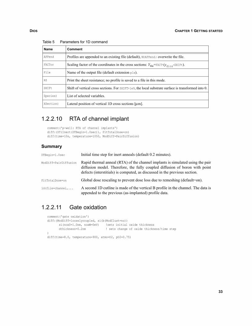
DIOS CHAPTER 1 GETTING STARTED
1.2.2.10 RTA of channel implantcomment('p-well: RTA of channel implants')diff:(DT(Inert(DTBegin=1.0sec)), FitTotalDose=on)diff(time=10s, temperature=1050, ModDiff=PairDiffusion)
Summary
DTBegin=1.0sec Initial time step for inert anneals (default 0.2 minutes).
ModDiff=PairDiffusion Rapid thermal anneal (RTA) of the channel implants is simulated using the pairdiffusion model. Therefore, the fully coupled diffusion of boron with pointdefects (interstitials) is computed, as discussed in the previous section.
FitTotalDose=on Global dose rescaling to prevent dose loss due to remeshing (default=on).
1d(file=channel,... A second 1D cutline is made of the vertical B profile in the channel. The data isappended to the previous (as-implanted) profile data.
1.2.2.11 Gate oxidationcomment('gate oxidation')diff:(ModDiff=looselycoupled, si(b(ModClust=no))
si(nox0=1.0nm, noxW=0eV) !sets initial oxide thicknessdthickness=0.2nm ! sets change of oxide thickness/time step
)diff(time=8.0, temperature=900, atmo=O2, pO2=0.75)
Table 5 Parameters for 1D command
Name Comment
APPend Profiles are appended to an existing file (default), NOAPPend: overwrite the file.
FACTor Scaling factor of the coordinates in the cross sections: Yfile=FACT⋅(ydios-SHIFt).
File Name of the output file (default extension plx).
RS Print the sheet resistance; no profile is saved to a file in this mode.
SHIFt Shift of vertical cross sections. For SHIFT>1e9, the local substrate surface is transformed into 0.
Species) List of selected variables.
XSection) Lateral position of vertical 1D cross sections [μm].
33
DIOSCHAPTER 1 GETTING STARTED
Summary
The thin oxide model of Massoud (an elaboration of the Deal–Grove equation) is used by default;oxidation rate is Si crystal orientation-dependent.
diff Establishes a new set of global defaults:ModDiff=looselycoupled selects the loosely coupled diffusion model (see thefollowing discussion)si:(b(ModClust=no)) switches off boron clustering in siliconsi:(nox0=1.0nm, noxW:=0eV) sets the native oxide thickness to 1 nmdthickness=0.2nm is maximal increase in oxide thickness per time step
1.2.2.12 Diffusion models in Dios
Diffusion models can be selected either globally:
DIFFusion:(ModDiff=PairDiffusion)
or for an individual diffusion step:
DIFFusion(time=10s, temperature=1050, ModDiff=PairDiffusion)
Point defect–assisted diffusion models in crystalline silicon assume the coupling between dopants andthe two principal point defect species (interstitials or vacancies). This coupling is described by threetypes of equation:
Transient clustering model for each dopant
Pair formation, ionization, and diffusion of pairs
Ionization and diffusion of unpaired point defects
Equilibrium (or transient) (de)clustering of dopants
Equilibrium (or transient) (de)clustering of point defects (storage of majority of point defectsgenerated as implantation damage in immobile <311> clusters with subsequent transientdissolution)
In the following discussion:
D is the diffusion coefficient and usually depends on the carrier concentrations.
CS is the concentration of substitutional doping, for example, BActive for boron.
CC is the carrier concentration (electrons (n) for donors and holes (p) for acceptors).
I0 is the concentration of neutral unpaired point defects. Identical driving forces and equations areassumed for interstitials and vacancies.
34
DIOS CHAPTER 1 GETTING STARTED
PairDiffusion
The PairDiffusion model is the most complete model in terms of the coupling effects between pointdefects and dopants. The main assumptions for the diffusion are:
Point defect–dopant pairs: mobile species, numerous charge states
Unpaired point defects: mobile species, numerous charge states
Unpaired dopant on lattice site (substitutional): immobile species, fully activated
The diffusion flux is given by . For example, for boron, the diffusionflux is given by .
The use of PairDiffusion is recommended if transient or nonlocal coupling between dopant species orpoint defects needs to be simulated, for example, for reverse short-channel effect simulation.
SemiCoupled
The main assumptions of the SemiCoupled model are:
Point defect–dopant pairs: mobile species, numerous charge states
Unpaired point defects: mobile species, numerous charge states
Unpaired dopant on lattice site (substitutional): immobile species, fully activated
These assumptions are the same as for PairDiffusion. However, the major difference is the cancellationof one driving force. For the PairDiffusion:
The second gradient is completely neglected in the SemiCoupled model and we obtain. For example, for boron, the flux is given by.
The main consequence of this definition of the driving force is the absence of diffusion if there is nodoping gradient, even if a gradient of point-defect concentration exists. In this case, the PairDiffusionmodel and the SemiCoupled model give different results. The parameter values are the same as for thePairDiffusion model. It is not recommend to use the SemiCoupled model, due to the rather arbitrarycancellation of a driving force. The model has been implemented mainly to understand the nonlinearcoupling and for comparison to the literature.
LooselyCoupled
Assumptions are:
Point defect–dopant pairs: not existing
Unpaired point defects: mobile species, numerous charge states
Unpaired dopant on lattice site (substitutional): mobile species, fully activated
j D CC( ) grad CS CC I0⋅ ⋅( )⋅–=j D p( ) grad BActive p I0⋅ ⋅( )⋅–=
j D CC( ) grad CS CC I0⋅ ⋅( )⋅–= D CC( ) I0 grad CS CC⋅( ) D CC( ) CS CC grad I0( )⋅ ⋅ ⋅–⋅ ⋅–=
j D CC( ) I0 grad CS CC⋅( )⋅ ⋅–=j D p( ) I0 grad BActive p⋅( )⋅ ⋅–=
35
DIOSCHAPTER 1 GETTING STARTED
These assumptions are fundamentally different from the two previous models. In this model, the balanceequations for both point defects and dopant species no longer contain dopant point defect pairs.However, the neutral unpaired point defect concentration remains as a factor outside of the gradient inthe driving force, similar to the SemiCoupled model. The model assumptions are consistent and motivatedempirically: the dopant diffusivity depends on the local point defect concentrations.
The diffusion flux is given by . For example, the boron flux is given by. The parameters for the LooselyCoupled model are the same as for the
Equilibrium and Conventional models. These parameters are distinct from the ones used in thePairDiffusion and SemiCoupled models. The LooselyCoupled model can be used to account for transientdiffusion behavior.
Equilibrium
Assumptions are:
Neutral point defect concentration: prescribed externally, for example, constant
Point defect dopant pairs: not existent
Unpaired point defects: not balanced; can be derived from assumed neutral point defects, carrierconcentrations and substitutional dopant concentrations
Unpaired dopant on lattice site (substitutional): mobile species, fully activated
This model can be derived from the LooselyCoupled model if the point defects are assumed to diffuse veryfast. For an inert diffusion, the constant boundary value of the neutral interstitial concentration extendsthrough the entire simulation domain. During oxidation steps, an inhomogeneous interstitial profile iscomputed, which depends on the local oxidation rate at a ‘nearby’ silicon surface.
The diffusion flux is given by .
For example, for boron, the diffusion flux is given by .
The assumptions for the diffusivity correspond to the assumptions made in SUPREM-III. The sameparameters as in the LooselyCoupled and Conventional models are used. The equilibrium model cannot beused to simulate transient or non-equilibrium coupled diffusion effects.
Conventional
The assumptions are:
Neutral point defect concentration: prescribed externally, for example, constant
Point defects dopant pairs: not existent
Unpaired point defects: not balanced.; can be derived from assumed neutral point defects, carrierconcentrations and substitutional dopant concentrations
Unpaired dopant on lattice site (substitutional): mobile species, fully activated
j D CC( ) I0 grad CS CC⋅( )⋅ ⋅–=j D p( ) I0 grad BActive p⋅( )⋅ ⋅–=
j D CC( ) I0 grad CS CC⋅( )⋅ ⋅–=
j D p( ) I0 grad BActive p⋅( )⋅ ⋅–=
36
DIOS CHAPTER 1 GETTING STARTED
The basic model assumptions are equivalent to the Equilibrium model. During oxidation steps, aninhomogeneous interstitial profile is computed, which depends on the local oxidation rate of a ‘nearby’silicon surface.
The diffusion flux is given by .
For example, for boron, the driving force is given by .
There are two major differences between the Conventional and Equilibrium models. In the Conventionalmodel, the diffusion equation for each single dopant is solved separately and a Gummel-like outeriteration process is used. (In the Equilibrium model, the full coupled Newton problem is solved.) Someconvergence problems may occur for diffusion in polysilicon with the Conventional model.
The second difference is the selection of empirical models for the dopant diffusivities. In theConventional model, for each dopant species, the model can be selected individually:
Diffusion(B(ModDif=Suprem-2|Suprem-3|FairTsai|DC|DEff))
In the Equilibrium model, for all dopants, a Suprem-3 diffusivity model is used always. Only thecoefficients can be modified.
General notes
Although the diffusion models are available for any temperature range, the default parameters are validfor temperatures greater than 600oC and are most reliable in the range 750–1250oC.
The initial values of the total concentrations of point defects and dopant species are defined or modifiedexternally, for example, during an ion implantation step. The total concentrations are solution variablesin the global system of balance equations (initial boundary value problem for the system of nonlinearparabolic partial differential equations for all dopant species to be solved on the mesh). The assumeddiffusion fluxes depend on the chosen diffusion model.
Given the total concentrations of point defects and dopant species, the concentrations of substitutionaldopants, neutral point defects, clusters, electrons and so on, (local solution variables) and theirderivatives with respect to the total concentrations are solved in a local Newton iteration for each of themesh points. The local system of equations is composed of nonlinear algebraic or ordinary differentialequations. The number and type of equations in the local system depends on the material and the chosenmodels (for example, clustering).
For all models except PairDiffusion and SemiCoupled, by default, an equilibrium arsenic clustering modelis assumed. For the PairDiffusion and SemiCoupled models, a transient boron (de)clustering model isselected by default.
For ModDiff=Conventional, the diffusion model can be specified individually for each material and dopantspecies. In crystalline silicon, the default model has been described above. In polycrystalline materials(Po, MS) a so-called two-stream model is used by default, which takes into consideration the effects ofgrain growth, and grain and grain boundary diffusion. For other materials, either a constant diffusivity(DEFF) or a concentration-dependent (DC) diffusivity is assumed.
j D CC( ) I0 grad CS CC⋅( )⋅ ⋅–=
j D p( ) I0 grad BActive p⋅( )⋅ ⋅–=
37
DIOSCHAPTER 1 GETTING STARTED
For all diffusion models other than Conventional, the same type of equation in crystalline silicon isselected and the type of equation for materials other than crystalline silicon is fixed; only the coefficientscan be modified. In polycrystalline materials, a two-stream model and, in other materials, aconcentration-dependent diffusivity are used.
1.2.2.13 Diffusion, oxidation, epitaxy, prebake
All high-temperature processes are controlled by the command DIFFusion. Temperature and processingtime or final thickness have to be specified. The parameter ATMOsphere describes the process atmosphere,by default an inert diffusion step is assumed.
DIFFusion(atmosphere=h2o,temperature=1000,time=100)
For a temperature ramp, either the rate of temperature change TempRate can be specified [K/minute]:
DIFFusion(TEmperature=(700.,1000.),TempRate=3)
or a list of time intervals and corresponding temperature values (one more than time intervals) can bespecified:
DIFFusion(Time=(60,20,30),TEmperature=(800,1000,1000,800))
The processing time can be defined also by specifying the rate of temperature change and thetemperatures at start and end of the process.
Predeposition
To simulate a predeposition from the gas phase, the doping element and concentration must be specified:
DIFF(Time=20min,Temperature=1000degC,ELEMent=As,Conc=1e20/cm3)
Oxidation
For oxidation processes, the target oxide thickness can be specified. The thickness is converted into anoxidation time (assuming an undoped wafer with no initial oxide):
DIFFusion(Temperature=1000degC,atmosphere=h2o2,thickness=200nm)
Constant high-doping concentrations in polysilicon layers required for enhanced oxidation rates can bespecified when the poly is deposited or in the DIFFusion command:
Diffusion(CC(PO(ELEMent=P,CONCentration=1e21/cm3))
The default oxidation model is O2Diffusion=Diffusion, and the diffusion of the oxidant(s) and reaction atthe silicon–oxide interface are computed.
38
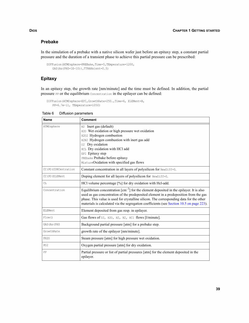
DIOS CHAPTER 1 GETTING STARTED
Prebake
In the simulation of a prebake with a native silicon wafer just before an epitaxy step, a constant partialpressure and the duration of a transient phase to achieve this partial pressure can be prescribed:
DIFFusion(ATMOsphere=PREBake,Time=5,TEmperature=1200,GAS(As(PHS=1E-10)),TTRANsient=0.5)
Epitaxy
In an epitaxy step, the growth rate [nm/minute] and the time must be defined. In addition, the partialpressure PP or the equilibrium Concentration in the epilayer can be defined:
DIFFusion(ATMOsphere=EPI,GrowthRate=250.,Time=6, ELEMent=B,PP=6.7e-11, TEmperature=1050)
Table 6 Diffusion parameters
Name Comment
ATMOsphere N2 Inert gas (default)H2O Wet oxidation or high pressure wet oxidationH2O2 Hydrogen combustionH2N2 Hydrogen combustion with inert gas addO2 Dry oxidationHCL Dry oxidation with HCl addEPI Epitaxy stepPREbake Prebake before epitaxyMixtureOxidation with specified gas flows
CC(PO(CONCentration Constant concentration in all layers of polysilicon for NewDiff=0.
CC(PO(ELEMent Doping element for all layers of polysilicon for NewDiff=0.
CL HCl volume percentage [%] for dry oxidation with Hcl-add.
Concentration Equilibrium concentration [cm–3] for the element deposited in the epilayer. It is also used as gas concentration of the predeposited element in a predeposition from the gas phase. This value is used for crystalline silicon. The corresponding data for the other materials is calculated via the segregation coefficients (see Section 10.5 on page 223).
ELEMent Element deposited from gas resp. in epilayer.
Flow() Gas flows of O2, H2O, H2, N2, HCl flows [l/minute].
GAS(As(PHS Background partial pressure [atm] for a prebake step.
GrowthRate growth rate of the epilayer [nm/minute].
PH2O Steam pressure [atm] for high pressure wet oxidation.
PO2 Oxygen partial pressure [atm] for dry oxidation.
PP Partial pressure or list of partial pressures [atm] for the element deposited in the epilayer.
39
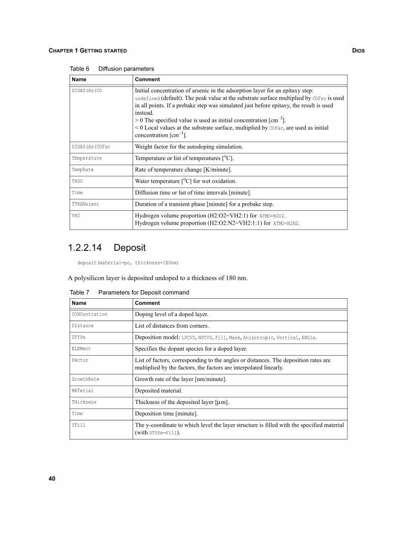
DIOSCHAPTER 1 GETTING STARTED
1.2.2.14 Depositdeposit(material=po, thickness=180nm)
A polysilicon layer is deposited undoped to a thickness of 180 nm.
SIGAS(As(CO Initial concentration of arsenic in the adsorption layer for an epitaxy step:undefined (default). The peak value at the substrate surface multiplied by COFac is used in all points. If a prebake step was simulated just before epitaxy, the result is used instead.> 0 The specified value is used as initial concentration [cm–3].< 0 Local values at the substrate surface, multiplied by COFac, are used as initial concentration [cm–3].
SIGAS(As(COFac Weight factor for the autodoping simulation.
TEmperature Temperature or list of temperatures [oC].
TempRate Rate of temperature change [K/minute].
TH2O Water temperature [oC] for wet oxidation.
Time Diffusion time or list of time intervals [minute].
TTRANsient Duration of a transient phase [minute] for a prebake step.
VH2 Hydrogen volume proportion (H2:O2=VH2:1) for ATMO=H2O2.Hydrogen volume proportion (H2:O2:N2=VH2:1:1) for ATMO=H2N2.
Table 7 Parameters for Deposit command
Name Comment
CONCentration Doping level of a doped layer.
DIstance List of distances from corners.
DTYPe Deposition model: LPCVD, NPCVD, Fill, Mask, Anisotropic, Vertical, ANGle.
ELEMent Specifies the dopant species for a doped layer.
FActor List of factors, corresponding to the angles or distances. The deposition rates are multiplied by the factors, the factors are interpolated linearly.
GrowthRate Growth rate of the layer [nm/minute].
MATerial Deposited material.
THickness Thickness of the deposited layer [μm].
Time Deposition time [minute].
YFill The y-coordinate to which level the layer structure is filled with the specified material (with DTYPe=Fill).
Table 6 Diffusion parameters
Name Comment
40
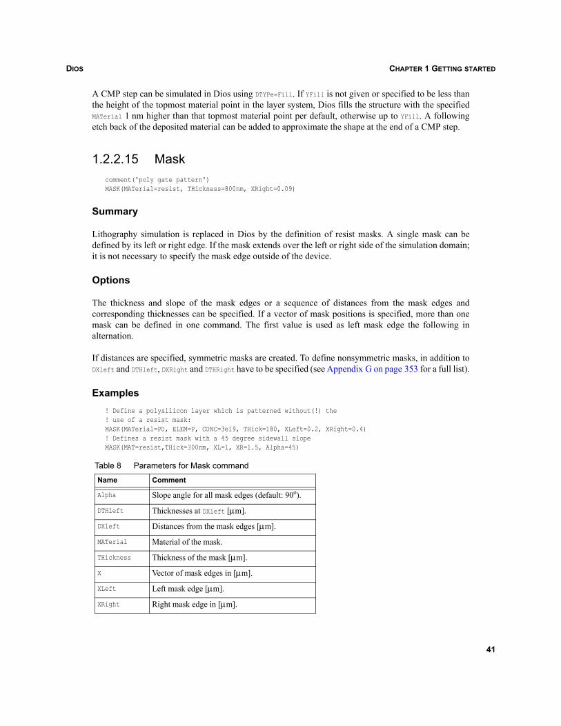
DIOS CHAPTER 1 GETTING STARTED
A CMP step can be simulated in Dios using DTYPe=Fill. If YFill is not given or specified to be less thanthe height of the topmost material point in the layer system, Dios fills the structure with the specifiedMATerial 1 nm higher than that topmost material point per default, otherwise up to YFill. A followingetch back of the deposited material can be added to approximate the shape at the end of a CMP step.
1.2.2.15 Maskcomment('poly gate pattern')MASK(MATerial=resist, THickness=800nm, XRight=0.09)
Summary
Lithography simulation is replaced in Dios by the definition of resist masks. A single mask can bedefined by its left or right edge. If the mask extends over the left or right side of the simulation domain;it is not necessary to specify the mask edge outside of the device.
Options
The thickness and slope of the mask edges or a sequence of distances from the mask edges andcorresponding thicknesses can be specified. If a vector of mask positions is specified, more than onemask can be defined in one command. The first value is used as left mask edge the following inalternation.
If distances are specified, symmetric masks are created. To define nonsymmetric masks, in addition toDXleft and DTHleft, DXRight and DTHRight have to be specified (see Appendix G on page 353 for a full list).
Examples! Define a polysilicon layer which is patterned without(!) the! use of a resist mask:MASK(MATerial=PO, ELEM=P, CONC=3e19, THick=180, XLeft=0.2, XRight=0.4)! Defines a resist mask with a 45 degree sidewall slopeMASK(MAT=resist,THick=300nm, XL=1, XR=1.5, Alpha=45)
Table 8 Parameters for Mask command
Name Comment
Alpha Slope angle for all mask edges (default: 90o).
DTHleft Thicknesses at DXleft [μm].
DXleft Distances from the mask edges [μm].
MATerial Material of the mask.
THickness Thickness of the mask [μm].
X Vector of mask edges in [μm].
XLeft Left mask edge [μm].
XRight Right mask edge in [μm].
41
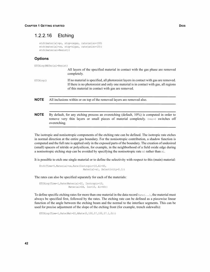
DIOSCHAPTER 1 GETTING STARTED
1.2.2.16 Etchingetch(material=po, stop=oxgas, rate(aniso=100)etch(material=ox, stop=sigas, rate(aniso=10))etch(material=Resist))
Options
ETCHing(MATerial=Resist)
All layers of the specified material in contact with the gas phase are removedcompletely.
ETCHing() If no material is specified, all photoresist layers in contact with gas are removed.If there is no photoresist and only one material is in contact with gas, all regionsof this material in contact with gas are removed.
NOTE All inclusions within or on top of the removed layers are removed also.
NOTE By default, for any etching process an overetching (default, 10%) is computed in order toremove very thin layers or small pieces of material completely. Over=0 switches offoveretching.
The isotropic and nonisotropic components of the etching rate can be defined. The isotropic rate etchesin normal direction at the entire gas boundary. For the nonisotropic contribution, a shadow function iscomputed and the full rate is applied only in the exposed parts of the boundary. The creation of undesired(small) spacers of nitride or polysilicon, for example, in the neighborhood of a field oxide edge duringa nonisotropic etching step can be avoided by specifying the nonisotropic rate A0 rather than A1.
It is possible to etch one single material or to define the selectivity with respect to this (main) material:
Etch(Time=5,Material=ox,Rate(Isotropic=10,A1=40,Material=si, Selectivity=0.1))
The rates can also be specified separately for each of the materials:
ETCHing(Time=1,Rate(Material=SI, Isotropic=10,Material=OX, Iso=10, A1=40))
To define specific etching rates for more than one material in the data record Rate(...), the material mustalways be specified first, followed by the rates. The etching rate can be defined as a piecewise linearfunction of the angle between the etching beam and the normal to the interface segments. This can beused for precise adjustment of the slope of the etching front (for example, trench sidewalls):
ETCHing(Time=1,Rate(Mat=SI,ARate(0,100,57,100,57.1,0)))
42
DIOS CHAPTER 1 GETTING STARTED
It is possible to specify several etching ‘beams’ (that is, directions). By default one single vertical beamis assumed:
ETCHing(Alpha(-7,7) Dose(0.5,0.5), SHadow(0.8,0.8)...)
1.2.2.17 Polysilicon reoxidationcomment('poly reoxidation')Replace(Control(ox(dx=2nm), MAsteps=10))! adjust stress dependent oxidation parametersdiffusion:(
ox(my0=2000poise ! default value=2093.1o2(Vd=6.0e-11um3)) ! default value=6.4e-11lmin=0.2nm, lmax=1nm)
diff(Temperature=(700,900),temprate=5,stressdep=on,kmin/kref=1.)diff(time=20,Temperature=900,atmo=O2, stressdep=on,kmin/kref=1)diff(Temperature=(900,700),temprate=5,stressdep=on,kmin/kref=1.)
Summary
Replace(Control(ox(dx=2nm), MAsteps=10))
Replaces the following Control parameters for oxide meshing:ox(dx=2nm) redefines the smallest triangle size allowed for grid adaptation in thegrowing oxide (may be smaller than the global dx).
Table 9 Parameters for Etching command
Name Comment
A0 Isotropic etching rate [nm/minute] applied only in the exposed part.
A1 Nonisotropic etching rate [nm/minute].
Alpha() List of directions of ‘etching beams’; 0: vertical, >0: from the left, <0: from the right.
Anisotropic Nonisotropic etching rate [nm/minute], launches strict vertical etching.
Arate() List of angles [degree] and rates [nm/minute] for piecewise linear etching rate.
Dose() Dose fraction (of 1.0) for the ‘etching beams’.
Isotropic isotropic etching rate [nm/minute].
Material Material for which etching rates are defined next.
MATerial (main) Etched material.
Rate( Data record of etching rates.
REmove Removed thickness of the material [μm].
Shadow) Shadow factor (0...1) used in the shadow of each ‘etching beam’.
SIGma Standard deviation of Gaussian distribution of the doses as function of the angle.
STOP Etch stop, name of either a material or a boundary sort.
Time Etching time [minute].
43
DIOSCHAPTER 1 GETTING STARTED
masteps=10 is the maximum number of time steps without readaptation (default30).
diffusion:(ox(my0=2000poise o2(vd=6.0e-11um3))
Globally adjusts the key coefficients controlling the effect of mechanical stresson the oxidation rate. As oxide grows at the bottom corner of the polysilicongate, it comes under increasing compressive stress. This stress causes a decreasein the diffusion of the oxidant species.
my0 Prefactor of the oxide viscosity (unit poise).
Vd ‘Activation volume’ [μm3] that controls the inverse exponential dependence ofthe oxidant diffusion coefficient on the pressure in the oxide.
diff(temperature=(700,900),temprate=5,stressdep=on,kmin/kref=1)
The temperature is ramped from 700oC to 900oC at a rate of 5oC/minute.
By default, an Uzawa scheme is used to compute the solution of the Stokes equation for the creepingflow of oxide and other materials of the overlayers during oxidation steps.
stressdep=on Switches on stress dependence (mechanical model) for the duration of anoxidation step.
kmin/kref=1 Switches off any influence of stress on oxidant reaction rate.
Options
misteps Minimum number of time steps without readaptation (default 2).
chsteps Number of time steps after which grid is checked for readaptation.
Additional parameters can be specified to describe the oxidation in detail:
DIFFusion(Temperature=900,Time=30,ATMOsphere=HCL,CL=3%)DIFFusion(Temperature=900,Time=30,Flow(O2=10l/min,HCl=0.3l/min))
NOTE The thickening of the oxide has been reduced by including mechanical stress effects. Theview is zoomed in using the left mouse button, and ‘equal scales’ are switched off using the=/!= button on the graphic display.
44
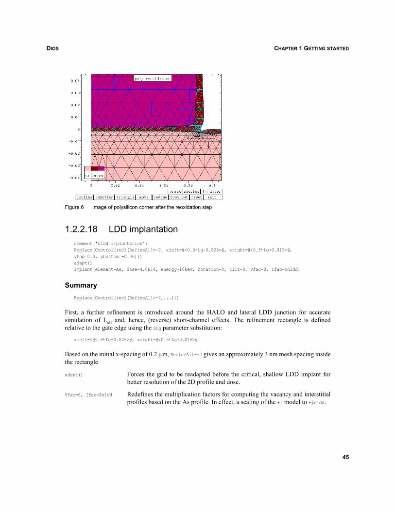
DIOS CHAPTER 1 GETTING STARTED
Figure 6 Image of polysilicon corner after the reoxidation step
1.2.2.18 LDD implantationcomment('nldd implantation')Replace(Control(rec1(RefineAll=-7, xleft=@<0.5*Lg-0.025>@, xright=@<0.5*Lg+0.015>@,ytop=0.0, ybottom=-0.06)))adapt()implant(element=As, dose=4.0E14, energy=10keV, rotation=0, tilt=0, Vfac=0, Ifac=$nldd)
SummaryReplace(Control(rec1(RefineAll=-7,...)))
First, a further refinement is introduced around the HALO and lateral LDD junction for accuratesimulation of Leff and, hence, (reverse) short-channel effects. The refinement rectangle is definedrelative to the gate edge using the $Lg parameter substitution:
xleft=<@0.5*Lg-0.025>@, xright=@<0.5*Lg+0.015>@
Based on the initial x-spacing of 0.2 μm, RefineAll=–7 gives an approximately 3 nm mesh spacing insidethe rectangle.
adapt() Forces the grid to be readapted before the critical, shallow LDD implant forbetter resolution of the 2D profile and dose.
Vfac=0, Ifac=$nldd Redefines the multiplication factors for computing the vacancy and interstitialprofiles based on the As profile. In effect, a scaling of the +1 model to +$nldd.
45
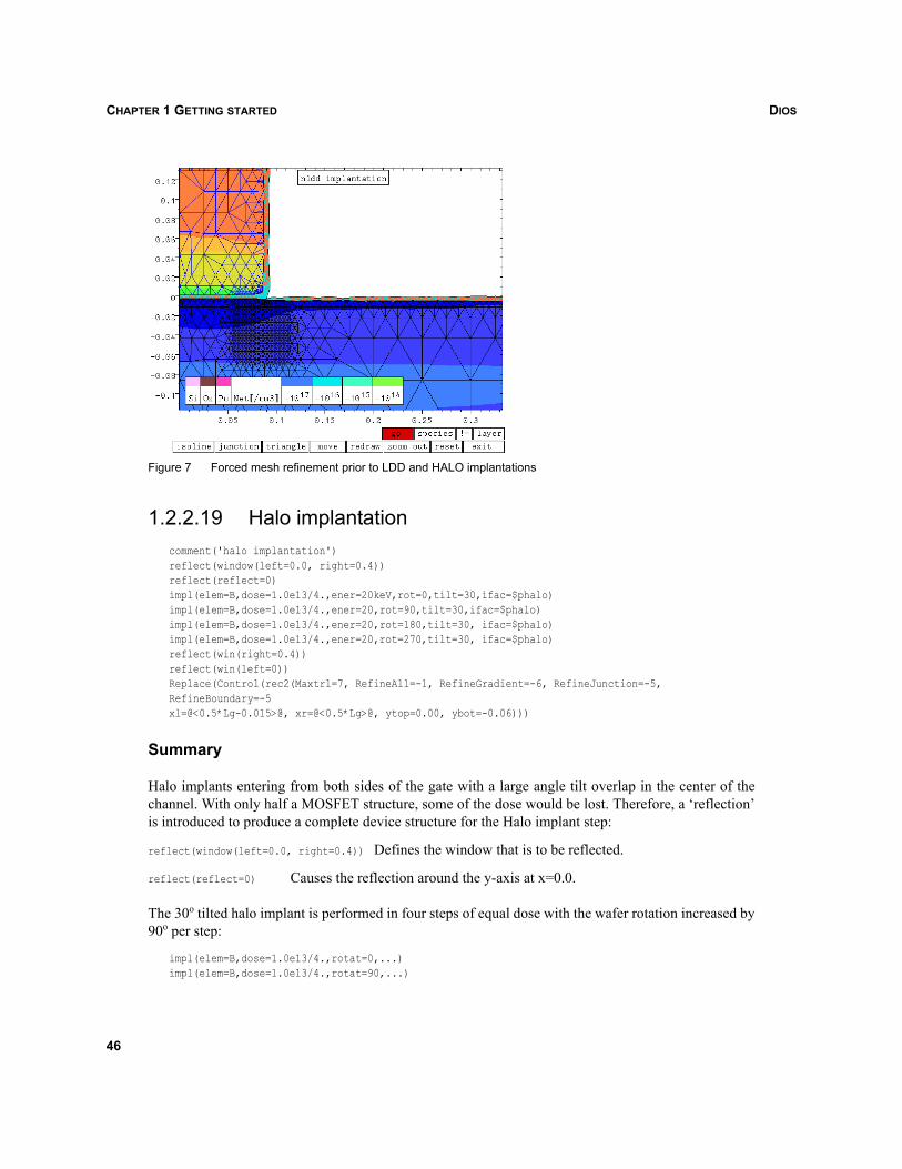
DIOSCHAPTER 1 GETTING STARTED
Figure 7 Forced mesh refinement prior to LDD and HALO implantations
1.2.2.19 Halo implantationcomment('halo implantation')reflect(window(left=0.0, right=0.4))reflect(reflect=0)impl(elem=B,dose=1.0e13/4.,ener=20keV,rot=0,tilt=30,ifac=$phalo)impl(elem=B,dose=1.0e13/4.,ener=20,rot=90,tilt=30,ifac=$phalo)impl(elem=B,dose=1.0e13/4.,ener=20,rot=180,tilt=30, ifac=$phalo)impl(elem=B,dose=1.0e13/4.,ener=20,rot=270,tilt=30, ifac=$phalo)reflect(win(right=0.4))reflect(win(left=0))Replace(Control(rec2(Maxtrl=7, RefineAll=-1, RefineGradient=-6, RefineJunction=-5, RefineBoundary=-5xl=@<0.5*Lg-0.015>@, xr=@<0.5*Lg>@, ytop=0.00, ybot=-0.06)))
Summary
Halo implants entering from both sides of the gate with a large angle tilt overlap in the center of thechannel. With only half a MOSFET structure, some of the dose would be lost. Therefore, a ‘reflection’is introduced to produce a complete device structure for the Halo implant step:
reflect(window(left=0.0, right=0.4)) Defines the window that is to be reflected.
reflect(reflect=0) Causes the reflection around the y-axis at x=0.0.
The 30o tilted halo implant is performed in four steps of equal dose with the wafer rotation increased by90o per step:
impl(elem=B,dose=1.0e13/4.,rotat=0,...)impl(elem=B,dose=1.0e13/4.,rotat=90,...)
46
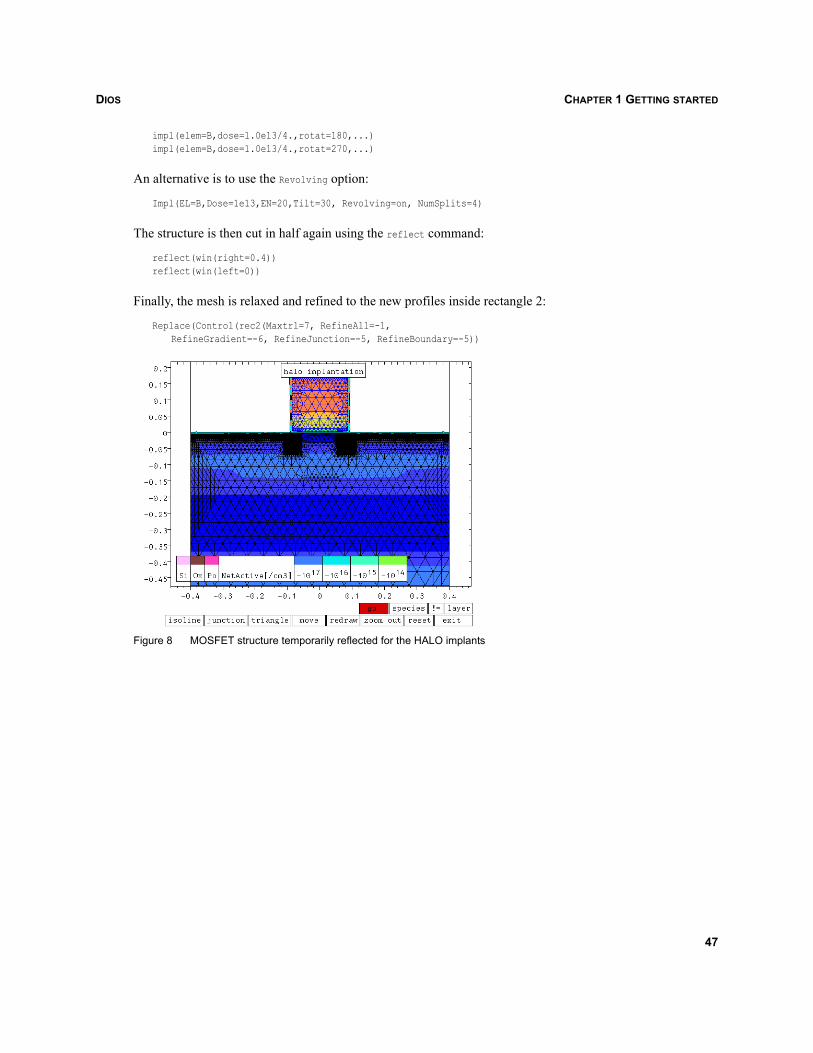
DIOS CHAPTER 1 GETTING STARTED
impl(elem=B,dose=1.0e13/4.,rotat=180,...)impl(elem=B,dose=1.0e13/4.,rotat=270,...)
An alternative is to use the Revolving option:
Impl(EL=B,Dose=1e13,EN=20,Tilt=30, Revolving=on, NumSplits=4)
The structure is then cut in half again using the reflect command:
reflect(win(right=0.4))reflect(win(left=0))
Finally, the mesh is relaxed and refined to the new profiles inside rectangle 2:
Replace(Control(rec2(Maxtrl=7, RefineAll=-1,RefineGradient=-6, RefineJunction=-5, RefineBoundary=-5))
Figure 8 MOSFET structure temporarily reflected for the HALO implants
47
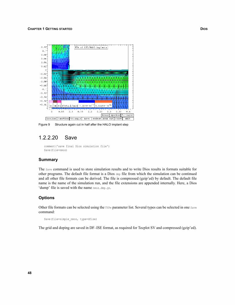
DIOSCHAPTER 1 GETTING STARTED
Figure 9 Structure again cut in half after the HALO implant step
1.2.2.20 Savecomment('save final Dios simulation file')Save(file=nmos)
Summary
The Save command is used to store simulation results and to write Dios results in formats suitable forother programs. The default file format is a Dios dmp file from which the simulation can be continuedand all other file formats can be derived. The file is compressed (gzip’ed) by default. The default filename is the name of the simulation run, and the file extensions are appended internally. Here, a Dios‘dump’ file is saved with the name nmos.dmp.gz.
Options
Other file formats can be selected using the TYPe parameter list. Several types can be selected in one Savecommand:
Save(file=simple_nmos, type=dfise)
The grid and doping are saved in DF–ISE format, as required for Tecplot SV and compressed (gzip’ed).
48
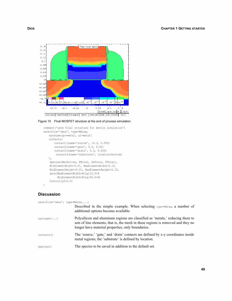
DIOS CHAPTER 1 GETTING STARTED
Figure 10 Final MOSFET structure at the end of process simulation
comment('save final structure for device simulation')save(file='nmos', type=Mdraw,
synonyms(po=metal, al=metal)contacts(
contact1(name='source', -0.3, 0.005) contact2(name='gate', 0.0, 0.05) contact3(name='drain', 0.3, 0.005) contact4(name='substrate', location=bottom)
), Species(NetActive, BTotal, AsTotal, PTotal), MinElementWidth=0.01, MaxElementWidth=0.10, MinElementHeight=0.01, MaxElementHeight=0.10, gate(MaxElementWidth=@<Lg/10.0>@ MinElementWidth=@<Lg/40.0>@) Control(y0=0.0))
Discussion
save(file='nmos', type=Mdraw,...)
Described in the simple example. When selecting type=Mdraw, a number ofadditional options become available:
synonyms(...) Polysilicon and aluminum regions are classified as ‘metals,’ reducing them tosets of line elements, that is, the mesh in these regions is removed and they nolonger have material properties, only boundaries.
contacts() The ‘source,’ ‘gate,’ and ‘drain’ contacts are defined by x-y coordinates insidemetal regions; the ‘substrate’ is defined by location.
species() The species to be saved in addition to the default set.
49
DIOSCHAPTER 1 GETTING STARTED
MinElementWidth=...etc. Defines global refinement criteria for Mdraw:gate(MaxElementWidth=@<Lg/10.0>@
MinElementWidth=@<Lg/40.0>@)
Defines refinement parameters inside a ‘gate box’ that is automatically locatedunder the poly gate. This provides extra channel refinement for MOSFETs.
Control(y0=0.0) Allows repositioning of the silicon–oxide interface along the y-axis. In thiscase, the topmost point of the silicon substrate surface is set to y=0.
1.2.2.21 LoadLoad(File='test')
The Load command is used to read a Dios save file for continuing the simulation or for graphicalrepresentation of the results. It can be used immediately after the Title command.
Alternatively, the Load command can also be used to read and interpolate ‘arbitrary’ doping profileswithout taking into account the current layer system (unlike the Implantation command). In this mode,GRID and Substrate commands must be predefined.
The following file formats can be selected: TYPe=plt, exp, prf, plx, Prosim, Relief, Tesim, Dios, XGraph, Mdraw.
In addition, analytic functions can be used to define the profiles, similar to what is performed typicallyin a device simulator: TYPe=Remove, Constant, Gauss, Erf, DIFfgaus, GAUSS3, LineGauss. For a detaileddescription of the file formats, applied analytic functions, and coordinate transformations, seeSection 2.10 on page 70.
1.2.2.22 PrintPrint(Layers)
Summary
The printout within the diffusion time steps is controlled by the parameters INFO, IPRNwt, and LPRot in thedata record Control. The larger these values are, the more output is produced. If INFO=1, technological andmodel parameters are printed. LPRot controls the printing of time, time step, dopant integrals andextremal values; IPRNwt controls the printing of the defect and error of Newton iterations. Values between0 and 2 can be used. For IPRNwt>2, INFO>2 very detailed information is printed to the protocol file.
Options
Print(Species(Net),Y(0,-1.),NY(10),X(0.,1.),NX(5), TABle) Prints a table of doping values.
Print(Alldata) Prints the model parameters of the last processing step(s). The printed outputcan be repeated after a certain number of time steps and at the end of any processstep if NPrint is set to a positive value: Replace(Control(NPrint=100)).
50
DIOS CHAPTER 2 SIMULATOR DIOS
Dios
CHAPTER 2 Simulator Dios
2.1 OverviewThe commands you can enter into a system shell or the Dios input shell are typed as:
dios show
or:
Implantation
Courier font is used for file names and file extensions that are used or created in Dios. The file types thatDios can create are usually distinguished in this text by their file extension, for example, .log file or .dmpfile. The types of file and their purposes are explained in Section 2.4 on page 54. Valid abbreviations areindicated in brackets (eval[uate]) and, sometimes, brackets indicate optional parameters that are notrequired to run Dios. Several possible values of a parameter or keyword selection are separated byvertical bars ( | ), for example, Diffusion(B(ModDif=Suprem-2|Suprem-3|FairTsai|DC|DEff)).
In the appendices, tables are provided, which contain all Dios parameters. Some parameters are outdatedand are kept only for test versions. Some may be useful only for special configurations of Dios. Theseparameters are not to be used in input files unless advised by the Synopsys Technical Support Center.
2.2 Start and stop, command-line argumentsTo start Dios, type:
dios [commands] [-log=xxx] [-mask=yyy] [parameters] [&]
When started, Dios opens the command file commands for reading commands. The command file is alwaysparsed twice. During the first pass, only the syntax of the commands in the file is checked and Diosopens further input files specified in the command file. If the first pass is finished and no errors aredetected, the command execution starts. If commands provides only a base name with no file extension andif no file commands is found, Dios opens one of the files commands.dio, commands.cmd, or commands_dio.cmd asa command file (in this given order). If the input file is specified as commands_dio.cmd, in addition to thefile extension, the _dio substring is stripped from the default base name of the files, searched or createdby Dios, in order to avoid _dio_dio constructions when saving files. If commands is not specified, dios_PIDis used as a base name.
If no command file is found, or syntax errors are detected, or errors occur during the execution of acommand, Dios enters the interactive mode. This mode is always indicated by the Dios input prompt inthe command window (that is, where Dios was started and where all the standard output is displayed).The input prompt is dios> on the main input level and command> on deeper command levels.
51
DIOSCHAPTER 2 SIMULATOR DIOS
Dios can be stopped (on each input level) with one of the commands exit, stop, bye, or end. Enter thesecommands at the beginning of the input line. Dios can also be stopped if a SIGQUIT signal (Ctrl+\) isentered in the command window or with clicking the exit button in the X11 graphics window. TheINTERRUPT signal (Ctrl+C) is caught in Dios to interrupt the simulation. It cannot be used to end a Diossimulation. Dios can also be used as a graphics tool to visualize its own result files. If a dmp file (Diosresult file) or a plx file (1D x-y plot file) is specified as commands, Dios reads the file and enters thegraphic command in the interactive command mode:
dios problem.dmp[|.gz|.Z] [-log=xxx] [&]dios problem.plx [-log=xxx] [&]
The dmp file can be gzip’ed, compressed, or uncompressed.
Several command-line options are allowed in Dios:
-t Run only syntax test of the specified command file.
-b Run in batch mode In batch mode, the X11 graphical output is suppressed. Ifthere is an error, the program stops without entering the interactive mode. Inbatch mode, the program does not need any window if the job is send to thebackground.
-h Start in help mode (see Section 2.5 on page 57).
-u Start in Sentaurus Workbench mode (X11 graphics output is enabled but nointeractive commands are allowed).
-v Print the current program version and compilation data only.
-o Old style interactive input (blocking read from standard input, X11 events areblocked if a command is expected).
-p Pipe mode (X11 graphics enabled, read from standard input through pipe, nocommand prompt).
-g Print all default parameter values to the file:defaults_versionNumber_compilationDate.dio
-G Print all default parameter values to the file:defaults_versionNumber_compilationDate.dio.Such files can be used to detect differences of command syntax with oldversions.
-help Print the list of command-line options only.
-Private Use a private color map.
-ASCII Use ASCII dmp files.
-redraw Automatically draw a new X11 picture when the graphics window is obscured.
-OldRead Use the reading function from old versions to scan input files.
-license=Dios|DiosSmall
Use a particular license feature to be checked out.
52
DIOS CHAPTER 2 SIMULATOR DIOS
-log=FILE Use FILE[.log] as protocol file.
-mask=FILE Use FILE[.tl1] as mask file.
-tmpdir=dir Use dir for temporary files.
-compat Execute a compatibility file to revert to the previous version after each titlecommand. These compatibility files are contained in the directory $STROOT_LIB/dioslib. The file switch_defaults_from_9.0_to_8.0.dio can be executed toreinforce as many of the default values of the preceding Dios version aspossible.
NOTE Not all implemented algorithms can be controlled from the input language and, therefore,some differences between different versions may remain. With the -compat command-lineflag, the ‘best match’ to the preceding Dios version can be expected.
-running 20.00 8.15 Run only in the specified wall clock time interval.
NAME=value Parameter values can be specified on the command line. These parameterassignments can be used as @<NAME>@ in Dios expressions in the commands fileor as NAME in expressions of Sentaurus Workbench that is, within @<...>@ or @...@.
NOTE These variables are overwritten if they appear in a set NAME=value statement in the input file.
-NAME=value Equivalent to NAME=value.
2.3 Geometry and mask positionsWhen you start the simulation of a new structure for the first time, a fast test run is recommended tocheck schematically the correctness of all mask positions, etching, oxidation, and doping. Incorrectmask specification is a common error. To obtain this test quickly, it is recommended to switch off thesimulation of dopant diffusion and to use a very coarse grid (which is good for this purpose only but notfor a meaningful simulation result). A picture can be drawn at the end of each process step and all savecommands can be switched off.
This can be performed after the Title command:
Title()Diff:(DopDiff=Off)Replace(Control(MaxTrl=1))Replace(Control(NGraphic=10000,NSave=-1)))
NOTE Remove these lines for the ‘real’ simulation run.
53
DIOSCHAPTER 2 SIMULATOR DIOS
2.4 Default file names and file extensionsBy default, the command lines are printed on standard output when Dios has parsed a line. When a Dioscommand is completed, the command is executed and generates further messages to standard output. Bydefault, Dios reports all error messages, warnings, and other messages to standard output in thecommand window and also writes everything to the log (or protocol) file. The log file is created in thecurrent working directory and its name is derived from the base name of the command file.
NOTE The input file names nxx_dio.cmd, nxx.dio, and nxx.cmd differ only in their file extension. Theyare all mapped to the same base name nxx, that is, the log file for all of them is named bydefault nxx.log.
Dios first erases the content of an existing log file and then writes the new log file. If Dios cannot writethe log file (for example, the user has no write permission), Dios prints a warning and tries to use the file/tmp/basename_PID.log instead.
NOTE Running the same example at the same time on different machines may lead to confusion ormay terminate one of the jobs. If so, specify different names for the log files on the commandline when starting Dios.
If Dios is running in Sentaurus Workbench, the input file is named nxx_dio.cmd. Dios does not generateany log file, but Sentaurus Workbench duplicates any Dios output (or its subprocesses) to standardoutput into a file named nxx_dio.out.
Dios checks errors when writing files. For example, if the disk is full while writing a dmp file, Dios doesnot continue the simulation but enters the interactive mode. The user can then clean up the disk space,save the file with an interactive command, and continue the simulation using the go command. If the diskbecomes full while writing into the log file, the simulation can continue, but the remaining part of thelog file may be incomplete or missing. If Dios is run in Sentaurus Workbench mode (flag -u), it cannotenter the command mode, but retries to save a file later (after sleeping some time).
Dios may generate several temporary files (dc_init_USER_PID, MC_USER_PID.*, *PID.tmp, andcommands_USER_PID*). All temporary files are created by default in the /tmp directory. The user can defineanother directory for the temporary files on the command line when starting Dios or by using theenvironment variable TMPDIR. Some temporary files (MC_USER_PID.*, commands_PID*) may be quite large,especially if 3D structures are simulated. If Dios terminates successfully, usually, the temporary files areremoved automatically; otherwise, they may have to be removed manually.
NOTE In Release 6.1, a dot ‘.’ was permitted to be used in file names. However, Dios no longer usesthis to recognize file extensions. Dios requires more precision with the provided fileextensions for the input files and appends the standard file extensions if they are missing. Fileextensions are case sensitive (same as file names) on all UNIX platforms.
54
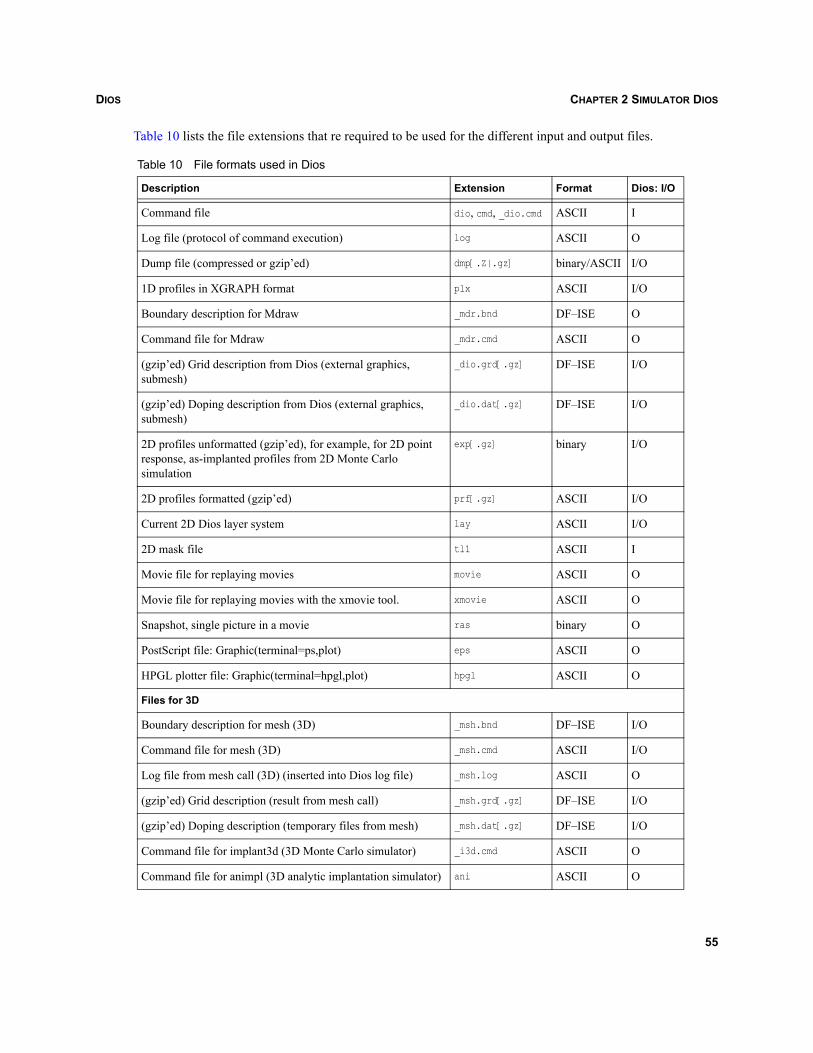
DIOS CHAPTER 2 SIMULATOR DIOS
Table 10 lists the file extensions that re required to be used for the different input and output files.
Table 10 File formats used in Dios
Description Extension Format Dios: I/O
Command file dio, cmd, _dio.cmd ASCII I
Log file (protocol of command execution) log ASCII O
Dump file (compressed or gzip’ed) dmp[.Z|.gz] binary/ASCII I/O
1D profiles in XGRAPH format plx ASCII I/O
Boundary description for Mdraw _mdr.bnd DF–ISE O
Command file for Mdraw _mdr.cmd ASCII O
(gzip’ed) Grid description from Dios (external graphics, submesh)
_dio.grd[.gz] DF–ISE I/O
(gzip’ed) Doping description from Dios (external graphics, submesh)
_dio.dat[.gz] DF–ISE I/O
2D profiles unformatted (gzip’ed), for example, for 2D point response, as-implanted profiles from 2D Monte Carlo simulation
exp[.gz] binary I/O
2D profiles formatted (gzip’ed) prf[.gz] ASCII I/O
Current 2D Dios layer system lay ASCII I/O
2D mask file tl1 ASCII I
Movie file for replaying movies movie ASCII O
Movie file for replaying movies with the xmovie tool. xmovie ASCII O
Snapshot, single picture in a movie ras binary O
PostScript file: Graphic(terminal=ps,plot) eps ASCII O
HPGL plotter file: Graphic(terminal=hpgl,plot) hpgl ASCII O
Files for 3D
Boundary description for mesh (3D) _msh.bnd DF–ISE I/O
Command file for mesh (3D) _msh.cmd ASCII I/O
Log file from mesh call (3D) (inserted into Dios log file) _msh.log ASCII O
(gzip’ed) Grid description (result from mesh call) _msh.grd[.gz] DF–ISE I/O
(gzip’ed) Doping description (temporary files from mesh) _msh.dat[.gz] DF–ISE I/O
Command file for implant3d (3D Monte Carlo simulator) _i3d.cmd ASCII O
Command file for animpl (3D analytic implantation simulator) ani ASCII O
55
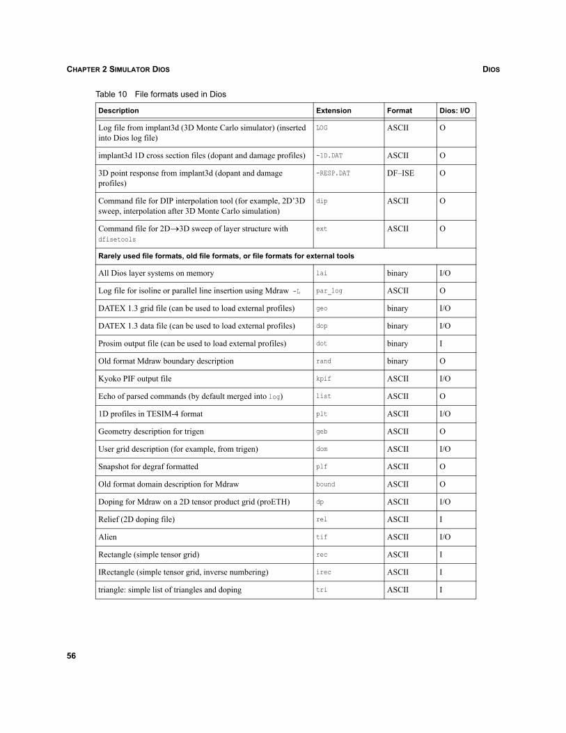
DIOSCHAPTER 2 SIMULATOR DIOS
Log file from implant3d (3D Monte Carlo simulator) (inserted into Dios log file)
LOG ASCII O
implant3d 1D cross section files (dopant and damage profiles) -1D.DAT ASCII O
3D point response from implant3d (dopant and damage profiles)
-RESP.DAT DF–ISE O
Command file for DIP interpolation tool (for example, 2D’3D sweep, interpolation after 3D Monte Carlo simulation)
dip ASCII O
Command file for 2D→3D sweep of layer structure with dfisetools
ext ASCII O
Rarely used file formats, old file formats, or file formats for external tools
All Dios layer systems on memory lai binary I/O
Log file for isoline or parallel line insertion using Mdraw -L par_log ASCII O
DATEX 1.3 grid file (can be used to load external profiles) geo binary I/O
DATEX 1.3 data file (can be used to load external profiles) dop binary I/O
Prosim output file (can be used to load external profiles) dot binary I
Old format Mdraw boundary description rand binary O
Kyoko PIF output file kpif ASCII I/O
Echo of parsed commands (by default merged into log) list ASCII O
1D profiles in TESIM-4 format plt ASCII I/O
Geometry description for trigen geb ASCII O
User grid description (for example, from trigen) dom ASCII I/O
Snapshot for degraf formatted plf ASCII O
Old format domain description for Mdraw bound ASCII O
Doping for Mdraw on a 2D tensor product grid (proETH) dp ASCII I/O
Relief (2D doping file) rel ASCII I
Alien tif ASCII I/O
Rectangle (simple tensor grid) rec ASCII I
IRectangle (simple tensor grid, inverse numbering) irec ASCII I
triangle: simple list of triangles and doping tri ASCII I
Table 10 File formats used in Dios
Description Extension Format Dios: I/O
56
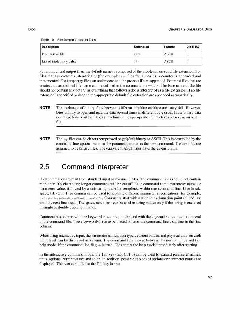
DIOS CHAPTER 2 SIMULATOR DIOS
For all input and output files, the default name is composed of the problem name and file extension. Forfiles that are created systematically (for example, ras files for a movie), a counter is appended andincremented. For temporary files, an underscore and the process ID are appended. For most files that arecreated, a user-defined file name can be defined in the command File="...". The base name of the fileshould not contain any dots ‘.’ as everything that follows a dot is interpreted as a file extension. If no fileextension is specified, a dot and the appropriate default file extension are appended automatically.
NOTE The exchange of binary files between different machine architectures may fail. However,Dios will try to open and read the data several times in different byte order. If the binary dataexchange fails, load the file on a machine of the appropriate architecture and save as an ASCIIfile.
NOTE The dmp files can be either (compressed or gzip’ed) binary or ASCII. This is controlled by thecommand-line option -ASCII or the parameter FORMat in the Save command. The exp files areassumed to be binary files. The equivalent ASCII files have the extension prf.
2.5 Command interpreterDios commands are read from standard input or command files. The command lines should not containmore than 200 characters; longer commands will be cut off. Each command name, parameter name, orparameter value, followed by a unit string, must be completed within one command line. Line break,space, tab (Ctrl+I) or comma can be used to separate different parameter specifications, for example,implantation(elem=B en=20keV,dose=1e15). Comments start with a # or an exclamation point (!) and lastuntil the next line break. The space, tab, #, or ! can be used in string values only if the string is enclosedin single or double quotation marks.
Comment blocks start with the keyword /* (or cbegin) and end with the keyword */ (or cend) at the endof the command file. These keywords have to be placed on separate command lines, starting in the firstcolumn.
When using interactive input, the parameter names, data types, current values, and physical units on eachinput level can be displayed in a menu. The command help moves between the normal mode and thishelp mode. If the command line flag -h is used, Dios enters the help mode immediately after starting.
In the interactive command mode, the Tab key (tab, Ctrl+I) can be used to expand parameter names,units, options, current values and so on. In addition, possible choices of options or parameter names aredisplayed. This works similar to the Tab key in tcsh.
Promis save file save ASCII I
List of triplets: x,y,value lis ASCII I
Table 10 File formats used in Dios
Description Extension Format Dios: I/O
57
DIOSCHAPTER 2 SIMULATOR DIOS
All commands read from a command file or the terminal are written into a file (by default this is mergedinto the protocol file (log) and are echoed at the terminal. The command System(Listing=File) directs thecommand output into a separate file (default file extension list). This file can be used later as commandfile for a subsequent Dios run.
Interactive commands are stored in a history buffer, which can be displayed with the hist or historycommand. The lines from the buffer can be reused as command lines by selecting them as in the shellwith an exclamation point (!) followed by a string or number identifier or with the arrow keys (this doesnot work for all window systems and shells). Only very poor command line editing is provided.
NOTE To ensure parallel reading of commands in the command window and reception of X11events, the terminal characteristics of the command window have been modified. This maynot work for all shells and window systems. (Use tcsh when starting Dios.) It may restrict thefunctionality of the Backspace or Delete keys for command-line editing or damage theterminal characteristics after leaving Dios. If Dios does not work properly, use the command-line option -o to prevent this modification. In this case, reading the command input will blockthe X11 event checking. If the program waits for input and does not react on X11 events, usersmust provide some input in the command window (for example, space) and press the Returnkey.
2.5.1 Syntax of input language
Parameter names have, at most, 24 characters. Except for file names, the Dios input language is not casesensitive. Dios does not change the case of user input. Always one parameter or one command is thecurrent one. In help mode, Dios prints a pointer (==>) in front of the current parameter or command. Ifjust a parameter name is entered, the appropriate parameter becomes current. For the current parameter,a value can be entered without a name or an equal sign (=). The value is assigned to the current parameterand the next parameter becomes current. This can be used to enter an array of values for example, x(1,2).
Parameter names can be abbreviated. Dios notifies the user (during the syntax test and the commandexecution) as to which name was used if the abbreviated name is ambiguous. If a portion of an input linecannot be interpreted as name, value, expression, or abbreviation, an attempt is made to detect parameternames or values from earlier Dios versions and to replace them by their corresponding names or valuesin the current Dios version. A notification is given to the user. Sometimes, such a replacement is notpossible. A syntax error will be indicated and the input file must be adjusted with an editor.
For all parameter types of Dios, the value undefined can be specified. It is often used to indicate if theparameter value has been specified by the user.
For each parameter, a current value and a default value are stored in Dios. When typing a command, firstthe current parameter values are replaced by the default values and then modified by the input:
implantation( ! all parameters are set to their default valueselement=B energy=20keV ! the specified values override the default) ! the command is executed
58
DIOS CHAPTER 2 SIMULATOR DIOS
The current value of a parameter can be changed as [name=]value. If the current value is reset, forexample, after erroneous input, type name=default. This can be used also to reset all parameters of astructure, as it is in:
title() subs() depo(material=ox) depo(material=ni) impl()graphic(triangle=on,material(si,ni),plotmaterial=default,plot)
A modified current value of a parameter is usually used only within the command for which it wasspecified, for example, element, material, or energy. There are a few exceptions (grid and memoryallocation) where this behavior is not useful.
The default value of a parameter can also be modified as [name]:=value or [name]:value.If the modifiedcurrent value is used as a new default value, type name:=current. The Replace command can be used tomodify the default values for frequently and globally used control parameters (see Appendix Q onpage 553), for example, Replace(Control(NGraphic=10)). When changing a default value, also the currentvalue is set to the new default.
NOTE Dios is not aware of an old default value after you change the default value. You cannotreinforce the (hard coded) intrinsic default values that were valid after Dios is started unlessyou start a new simulation (either after exiting and restarting Dios, or after using the resetcommand in the same Dios session).
NOTE Some default values depend on the crystal orientation of the wafer, which is defined only inthe Substrate command. These default values cannot be changed before the Substratecommand was executed. Any such change is lost when executing the Substrate command.
2.5.1.1 Variables
In Dios, variables can be defined with the set name=value command. The names and values can also bedefined on the command line as name=value. The symbolic parameter names can be used in expressionsor when assigning values to input parameters. In Dios, @VAR@, @<VAR>@, and $VAR are equivalent.
2.5.1.2 Expressions
Values for integer, real, physical, or character parameters can be specified as an expression. Variablesare replaced by their (string) value. For character type parameters (file names, strings), concatenation isperformed (no special concatenation operator is required, for example, file=aa$VAR). For integerparameters, the algebraic operations (+, –, *, /) are supported. For real parameters, in addition, a power** is foreseen. The constants pi, k, and e are predefined (that is, e**$a is allowed). No parentheses areadmitted in expressions. You can only assign the value of a subexpression to another intermediatevariable. Otherwise, the syntax of expressions of Sentaurus Workbench is supported. The differentparameter types allow or require different input.
59
DIOSCHAPTER 2 SIMULATOR DIOS
2.5.1.3 Integer
Integer can be typed as usual. Expressions can be specified. All operands must be integers.
2.5.1.4 Real
Real can be typed as usual (1, –1e12). Expressions can be specified. All operands are interpreted as realnumbers.
2.5.1.5 Boolean
Boolean can be defined as true by specifying one of 1, true, wahr, ja, yes, t, w, j, on. They are defined asfalse by setting one of 0, false, f, no, n, off. Usually, they are defined true by typing their name and falseby typing NOname. In the help mode, on or off will be shown. No expressions are supported.
2.5.1.6 String
String can be entered with single or double quotation marks, or without quotation marks. If the stringcontains characters that are used as word delimiters in Dios (colon, comma, exclamation point,parentheses, braces, brackets, equal sign, space, tab Ctrl+I), the string must be enclosed in a pair ofsingle or double quotation marks ('abc:def'). If the quotation character itself is to be contained in thestring, use either the other type of quotation mark or type the quotation character twice with no space in-between. String expressions can be used, for example, file='abc'$base. No concatenation operator isrequired.
2.5.1.7 File name
There is a special data type for file names. Similar rules as for string input are used. A full path name ora relative path name can be specified. If no path name is included, the current working directory is used.A slash ‘/’ character is interpreted as separator between (sub)directory names and the base name of afile. If possible, avoid space and tab characters in file names. The dot ‘.’ character is allowed in filenames (see Section 2.4 on page 54).
2.5.1.8 Option
Option is a parameter type whose values are a list of keywords. In the interactive mode, the possiblevalues are displayed with the Tab key: name=Tab. The current value and all possible values are displayed.The value can also be changed with the operations =next, =previous, =first, =last. Internally, options arerepresented by integers. These numbers are also accepted on input, although this is not recommended.Physical units, the topology of Dios grids and layer systems, the regions, boundary lines, the Diosdatasets, materials and boundary sorts are special options. No expressions are supported.
60
DIOS CHAPTER 2 SIMULATOR DIOS
2.5.1.9 Physical parameters
In Dios, physical quantities are defined and printed with units. The input values can be specified withunits. This is highly recommended. There must be no space or tab between the value and unit. If no unitis specified, a default unit is assumed. The input values are scaled and the output is printed with thedefault unit. (For a list of units and default units, see Section 2.7 on page 65.) The default units are alsoused in the graphical output. The default unit can be changed: System(Time=sec, Thickness=nm,
Distance=nm, Length=nm).
The system command can be specified on the main command level after the title command in acommand file. It can also be used on each command level in the interactive command input (only in thefirst column of a continued command line):
dios> Graphic(plotGraphic> system(length=nm) plot)
Expressions can also be used to define values for physical parameters. In expressions for physicalparameters, all terms have to be either numbers or belong to the same physical quantity. Some terms inan expression may be given with no unit and some may have different units (for example, a=1 mm-3 nm+4).First, all terms in an expression are transformed to the internal default unit and the unit strings areremoved. Then, the numeric expression is evaluated as an expression for a real parameter and the resultis interpreted in the default unit of the parameter: mask(xleft=$SDMask+2um).
NOTE When changing a default unit, all subsequent input uses the modified unit for the appropriateparameter type unless the input is supplied with another unit.
NOTE To avoid the most frequent input error, thicknesses and distances are not accepted without aunit unless the value is less than 5.
All Dios parameters are grouped in different structures: Package, Record, Procedure, and Task. Eachstructure has a name. They differ in the action the program performs when opening or closing thestructures. Structures are opened and closed as: [name](...) or [name]=(...).
If for a structure name the input name=value is specified, this input is interpreted as ‘open the structure,assign value to the first parameter of the structure, and close the structure.’
2.5.1.10 Procedure
Procedure contains all parameters of a command. When opening a procedure, all parameters are set totheir default values. Then, the input is interpreted. When closing the procedure, the command isexecuted. A procedure without any parameter is executed if its name is entered.
61
DIOSCHAPTER 2 SIMULATOR DIOS
2.5.1.11 Task
A task also defines a command. On opening a task, a specific parameter initialization is performed.Unlike for a procedure, perhaps not all parameters are reset to their default values, or some parametersare set to zero or undefined values.
2.5.1.12 Package
Package is a group of parameters. Additional operations are not performed on opening or closing.
2.5.1.13 Record
Record differs from a package only with respect to the initialization. A subrecord of a procedure isinitialized, a subpackage is not. Vectors of parameters are treated as records. The operations =default and:=current are allowed also for structures. The specified operation is performed on all parameters andsubrecords of the structure.
2.5.1.14 Default values
Default values of parameters in a structure are modified if the structure is opened with a colon andparenthesis ‘:(’ instead of a parenthesis ‘(’. All input until the next matching closing parenthesis ‘)’ isinterpreted as ‘change default values.’ You do not need to specify colons everywhere. When opening acommand with ‘:(’, the command is not executed, only the current and default values are changed:
diff:(si(as(ModClust=Solubility)))
NOTE Default values that depend on the crystal orientation of the wafer and are not defined for eachof the three main crystal orientations <100> <110> <111> can be changed only after thecrystal orientation is specified in the command Substrate(Orientation=100).
2.5.2 Interpreter control commands
There are a few commands to control the command interpreter. These commands must be placed onseparate command lines and start in the first column. No abbreviations are allowed.
@FILENAME Switches input to FILENAME[.dio|.cmd|_dio.cmd].
@FILENAME goto 123 Switches input to FILENAME[.dio|.cmd|_dio.cmd], skips the input lines 1…122,and continues reading commands in line 123.
@FILENAME goto LABEL Switches input to FILENAME[.dio|.cmd|_dio.cmd], skips the first input linesincluding the line containing the string LABEL, and continues reading commands.
62
DIOS CHAPTER 2 SIMULATOR DIOS
break Interrupts reading from the command file and enters the interactive mode.
step Reads the next line from the command file. If a command is completed, it isexecuted and the interactive mode is entered again.
go Leaves interactive mode and continues reading and executing commands fromthe command file.
cont Same as go.
cancel Cancels reading from the command file.
echo abc Prints the value of variable abc. If no variable name is specified, print the valuesof all variables.
eval[uate] expr Evaluates an expression and print the result, for example, eval $b*2+3.
evaluate a=expression Defines the value of the variable to be the result of the expression.
set a=val Defines the value for the variable a (can be numeric value or a string).
define a=val Same as set a=val.
help Switches between help mode and normal mode.
top Moves to the first parameter (in the help mode).
pageup Moves one page up (in help mode).
pagedown Moves one page down (in help mode).
up Moves one line up (in help mode).
down Moves one line down (in help mode).
bottom Moves to the last parameter (in help mode).
cbegin Beginning of a comment block.
/* Same as cbegin.
cend End of a comment block.
*/ Same as cend.
sh Starts a new shell (and executes the UNIX commands following the keyword).Alternatively, tcsh, csh, or dcl can be used.
quit Leaves the current input level with no execution (if possible) or (on top level)leave Dios.
stop Leaves Dios. Alternatively, bye, end, or exit can be used.
To move around in the help mode, use the cursor keys, the help key and the F keys (Help: switches helpmode, F1: top, F2: pagedown, F3: pageup, F4: bottom, F5: =first, F6: =last, F7: =default, F8: :current,→: =next, ←: =previous, ↓: down, ↑: up). This may not work for all window systems or shells.
63
DIOSCHAPTER 2 SIMULATOR DIOS
The syntax of the command file, which was defined on the command line when starting Dios, is testedautomatically. To test and then execute other command files in an interactive session, use the followingcommands:
system(noexecute)@filename.diosystem(execute)@filename.dio
2.5.3 Preprocessor commands
Dios allows the use of some preprocessor-like control commands. All lines starting with the prefix # areinterpreted as containing only preprocessor directives. They can be used to multiply or omit parts of theinput file during the initial syntax check of the command file.
The Dios preprocessor has conditional directives as #if, #elif, #else, and #endif. Also possible arelooping directives using #do and #enddo. The following example demonstrates the use of preprocessordirectives:
#do SPECIES=As B Ge N PTITle("Preprocessor example")SUBStrate(ELEMent=@<SPECIES>@ Concentration=1e14)DIFFusion:(Si:(@<SPECIES>@:(#if @<SPECIES>@=As PV00=5.0e-37#elif @<SPECIES>@=B PV0PP=1.0e-37#else PV0MM=5.0e-30#endif)))reset()#enddoend
NOTE The reset statement before the #enddo is important. This ensures the reset of all default valuesbefore a new TITle statement, which is recommended for a new run of Dios.
2.5.4 System commands
The following parameters in the System command are used to control the simulator behavior.
Execute On – Commands are executed. Off – Syntax check.
Fullscr On – Help mode. Off – Normal mode.
Listing File name for protocol of interpreted commands.
Listunit Output unit for protocol of interpreted commands. By default, the commandsare listed in the Dios protocol file (Fortran input/output unit 4).
64
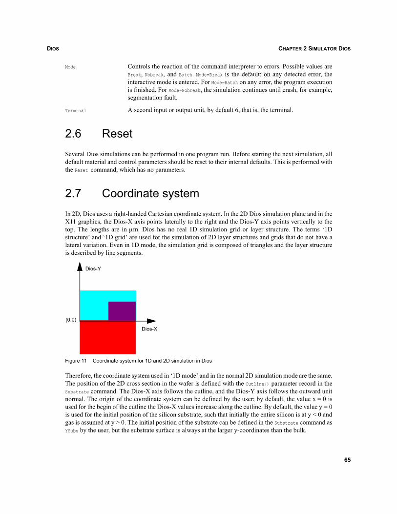
DIOS CHAPTER 2 SIMULATOR DIOS
Mode Controls the reaction of the command interpreter to errors. Possible values areBreak, Nobreak, and Batch. Mode=Break is the default: on any detected error, theinteractive mode is entered. For Mode=Batch on any error, the program executionis finished. For Mode=Nobreak, the simulation continues until crash, for example,segmentation fault.
Terminal A second input or output unit, by default 6, that is, the terminal.
2.6 ResetSeveral Dios simulations can be performed in one program run. Before starting the next simulation, alldefault material and control parameters should be reset to their internal defaults. This is performed withthe Reset command, which has no parameters.
2.7 Coordinate systemIn 2D, Dios uses a right-handed Cartesian coordinate system. In the 2D Dios simulation plane and in theX11 graphics, the Dios-X axis points laterally to the right and the Dios-Y axis points vertically to thetop. The lengths are in μm. Dios has no real 1D simulation grid or layer structure. The terms ‘1Dstructure’ and ‘1D grid’ are used for the simulation of 2D layer structures and grids that do not have alateral variation. Even in 1D mode, the simulation grid is composed of triangles and the layer structureis described by line segments.
Figure 11 Coordinate system for 1D and 2D simulation in Dios
Therefore, the coordinate system used in ‘1D mode’ and in the normal 2D simulation mode are the same.The position of the 2D cross section in the wafer is defined with the Cutline() parameter record in theSubstrate command. The Dios-X axis follows the cutline, and the Dios-Y axis follows the outward unitnormal. The origin of the coordinate system can be defined by the user; by default, the value x = 0 isused for the begin of the cutline the Dios-X values increase along the cutline. By default, the value y = 0is used for the initial position of the silicon substrate, such that initially the entire silicon is at y < 0 andgas is assumed at y > 0. The initial position of the substrate can be defined in the Substrate command asYSubs by the user, but the substrate surface is always at the larger y-coordinates than the bulk.
(0,0)
Dios-X
Dios-Y
65
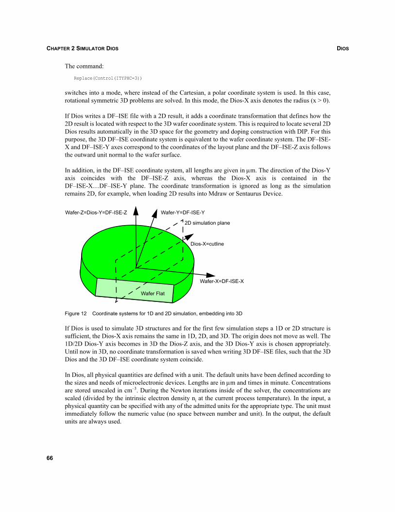
DIOSCHAPTER 2 SIMULATOR DIOS
The command:
Replace(Control(ITYPHC=3))
switches into a mode, where instead of the Cartesian, a polar coordinate system is used. In this case,rotational symmetric 3D problems are solved. In this mode, the Dios-X axis denotes the radius (x > 0).
If Dios writes a DF–ISE file with a 2D result, it adds a coordinate transformation that defines how the2D result is located with respect to the 3D wafer coordinate system. This is required to locate several 2DDios results automatically in the 3D space for the geometry and doping construction with DIP. For thispurpose, the 3D DF–ISE coordinate system is equivalent to the wafer coordinate system. The DF–ISE-X and DF–ISE-Y axes correspond to the coordinates of the layout plane and the DF–ISE-Z axis followsthe outward unit normal to the wafer surface.
In addition, in the DF–ISE coordinate system, all lengths are given in μm. The direction of the Dios-Yaxis coincides with the DF–ISE-Z axis, whereas the Dios-X axis is contained in theDF–ISE-X…DF–ISE-Y plane. The coordinate transformation is ignored as long as the simulationremains 2D, for example, when loading 2D results into Mdraw or Sentaurus Device.
Figure 12 Coordinate systems for 1D and 2D simulation, embedding into 3D
If Dios is used to simulate 3D structures and for the first few simulation steps a 1D or 2D structure issufficient, the Dios-X axis remains the same in 1D, 2D, and 3D. The origin does not move as well. The1D/2D Dios-Y axis becomes in 3D the Dios-Z axis, and the 3D Dios-Y axis is chosen appropriately.Until now in 3D, no coordinate transformation is saved when writing 3D DF–ISE files, such that the 3DDios and the 3D DF–ISE coordinate system coincide.
In Dios, all physical quantities are defined with a unit. The default units have been defined according tothe sizes and needs of microelectronic devices. Lengths are in μm and times in minute. Concentrationsare stored unscaled in cm–3. During the Newton iterations inside of the solver, the concentrations arescaled (divided by the intrinsic electron density ni at the current process temperature). In the input, aphysical quantity can be specified with any of the admitted units for the appropriate type. The unit mustimmediately follow the numeric value (no space between number and unit). In the output, the defaultunits are always used.
Wafer-X=DF-ISE-X
Wafer-Y=DF-ISE-YWafer-Z=Dios-Y=DF-ISE-Z
2D simulation plane
Dios-X=cutline
Wafer Flat
66
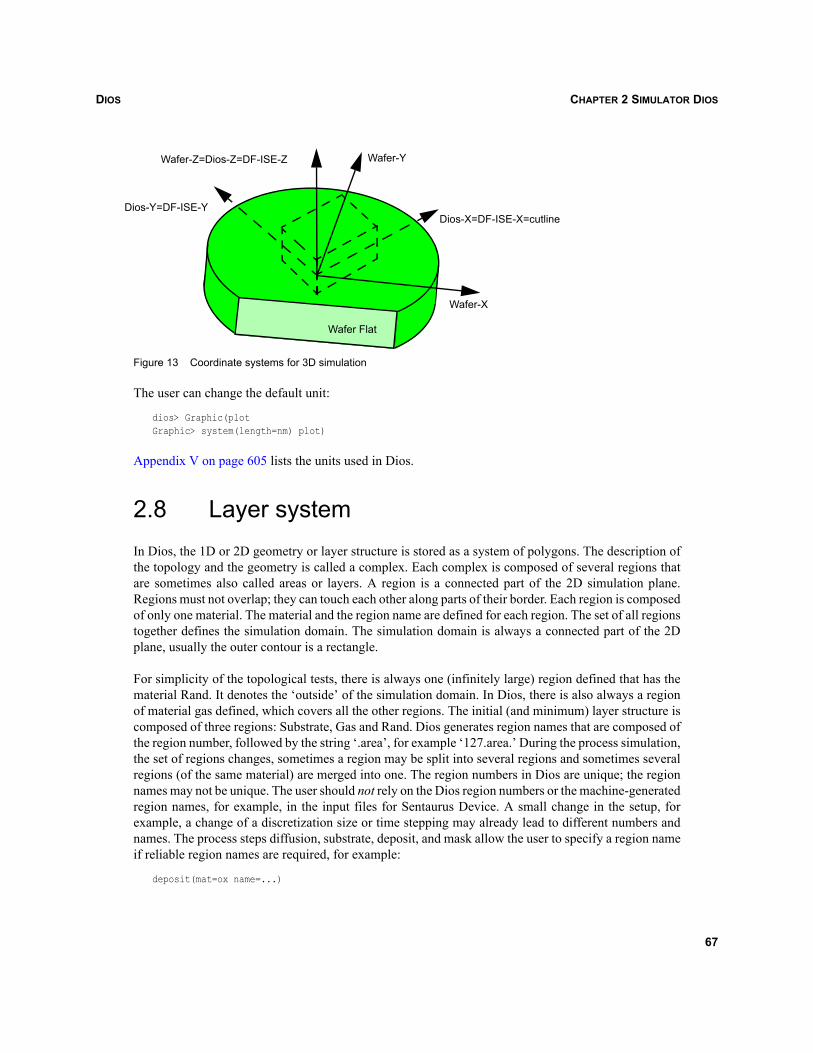
DIOS CHAPTER 2 SIMULATOR DIOS
Figure 13 Coordinate systems for 3D simulation
The user can change the default unit:
dios> Graphic(plotGraphic> system(length=nm) plot)
Appendix V on page 605 lists the units used in Dios.
2.8 Layer systemIn Dios, the 1D or 2D geometry or layer structure is stored as a system of polygons. The description ofthe topology and the geometry is called a complex. Each complex is composed of several regions thatare sometimes also called areas or layers. A region is a connected part of the 2D simulation plane.Regions must not overlap; they can touch each other along parts of their border. Each region is composedof only one material. The material and the region name are defined for each region. The set of all regionstogether defines the simulation domain. The simulation domain is always a connected part of the 2Dplane, usually the outer contour is a rectangle.
For simplicity of the topological tests, there is always one (infinitely large) region defined that has thematerial Rand. It denotes the ‘outside’ of the simulation domain. In Dios, there is also always a regionof material gas defined, which covers all the other regions. The initial (and minimum) layer structure iscomposed of three regions: Substrate, Gas and Rand. Dios generates region names that are composed ofthe region number, followed by the string ‘.area’, for example ‘127.area.’ During the process simulation,the set of regions changes, sometimes a region may be split into several regions and sometimes severalregions (of the same material) are merged into one. The region numbers in Dios are unique; the regionnames may not be unique. The user should not rely on the Dios region numbers or the machine-generatedregion names, for example, in the input files for Sentaurus Device. A small change in the setup, forexample, a change of a discretization size or time stepping may already lead to different numbers andnames. The process steps diffusion, substrate, deposit, and mask allow the user to specify a region nameif reliable region names are required, for example:
deposit(mat=ox name=...)
Wafer-X
Wafer-YWafer-Z=Dios-Z=DF-ISE-Z
Dios-Y=DF-ISE-YDios-X=DF-ISE-X=cutline
Wafer Flat
67
DIOSCHAPTER 2 SIMULATOR DIOS
If two regions of the same material are to be merged, for example, deposition of oxide on top of oxide,the name of the resulting region can be controlled by:
replace(control(RegionOrder=...
If both deposit commands specify a region name and RegionOrder=NewRegion is chosen (default), theregion name in the latter command determines the region name of the merged region. ForRegionOrder=PrevRegion, the opposite is the case. If one of the names is machine generated, then themerged region always has the user-specified name. Internally, machine-generated names are identifiedby a dot ‘.’ in the name (for example, 127.area). The switches RegionOrder=OldScheme andRegionOrder=undefined restore the behavior of Release 7.5. If a region is subdivided into two or moreregions during a process step (for example, etching, reflect), all of the new generated regions have thesame region name, the region name of the original region. User-specified region names are restricted toeight characters in length and should not contain a dot. Region names can be depicted in the graphicswith the command:
graphic(isoline=no layer=area longtext=on)
When saving a structure in Mdraw format, different regions with the same name must be renamed (seeSection 12.2.1 on page 285).
The border of each area is stored as a list of boundaries. A boundary belongs to only one area. It has acounterpart in the neighboring area, that is, on the ‘other’ side. The two boundaries belong to one line.A line is a connected set of straight line segments; a line can be an open or a closed polygon. For eachline, the ‘left’ and ‘right’ boundaries are known. The discretization of the line is given by a list of points.For each point on a line, the coordinates and the two neighboring points are known. Lines can only beginand end in ‘triple’ points, which are also called vertex, even if the line is a closed polygon. For eachvertex, the list of lines sharing the vertex is known. More than three lines can share a vertex (usuallythree, at least two). For each line, the name and the boundary sort are stored. A line represented by aclosed polygon defines an inclusion, which is an area completely surrounded by one other area.
To enable proper work of the topology algorithms, such inclusions are always connected to the mainlayer system by a line of a special type: the left and right boundaries of the line belong to the same area.Such lines are called imaginary because they are usually not drawn, when the set of lines is drawn.
As an illustration, type in the few lines below and compare the pictures:
title()subs()depo(ox,thick=0.1)mask(mat=po,x(-0.5,0.5),thick=0.2)depo(mat=ox,thick=0.1)graphic(isoline=no, junction=no, plot)graphic(layer=line, plot)graphic(layer=line, IMAGline=on, plot)end
68
DIOS CHAPTER 2 SIMULATOR DIOS
2.9 Grid (mesh)The simulation of doping profiles always requires a grid (also called mesh or triangulation). The meshgeneration process for the 1D and 2D Dios grids is described in Chapter 4 on page 79. A description of3D mesh generation can be found in the Mesh manual. In this section, only the basic terms, definitions,and relationships are defined.
For 1D and 2D structures, the Dios simulation mesh is composed of triangles only. The triangles arecalled elements of the mesh; the three sides of a triangle are called edges; the three corners are calledvertices (or nodes or mesh points) of the triangle. Triangles are not allowed to overlap, and no mesh pointmust be contained inside of a triangle or an edge. An edge is shared by one or two triangles. Edges sharedby only one triangle are called external edges of the mesh. Triangles sharing one edge are calledneighbors of each other and of the edge. Triangles of the mesh must belong entirely to one material.
The maximum set of neighboring triangles of the same material forms a region or an area of the mesh.A material interface is a connected set of edges that separates two regions of the mesh; an externalboundary is a connected set of external edges that are shared by triangles of the same region. Materialinterfaces and external boundaries are called lines of the mesh. A line of the mesh can only begin or endin a mesh point. Such mesh points are called ‘triple’ points of the mesh. At least two lines, usually three,share a ‘triple’ point; usually these points are shared by triangles of three different regions. Due to thelarge similarity to the layer structure, the topology description of a 2D mesh is described also by acomplex.
NOTE The 2D mesh does not contain imaginary lines. Usually, the mesh does not contain interfacesbetween regions of the same material, even if these interfaces are contained in the layerstructure (for example, if the user specifies names for both regions).
For a 3D simulation, the simulation mesh is composed of bricks, triangular prisms, pyramids, andtetrahedra. These objects are called elements of the mesh, and their sides are called faces of the element.Faces are triangles or rectangles, that is, planar objects in the 3D Euclidean space. The line segmentsthat compose the boundary of the faces are called edges of the face and of the elements sharing the face.The edges of an element are shared by two of its faces. The corners of the elements are called meshpoints (or vertices of the element). The mesh points of an element are shared by three of its faces andthree of its edges.
Elements are not allowed to overlap, and no mesh point must be contained inside of an element, face, oredge. A face is shared by one or two elements. Faces shared by only one element are called external orouter faces (of the element and of the mesh). Elements sharing one face are called neighbors of eachother, of the face, of all edges of the face and all vertices of these edges. Each element of the mesh mustbelong entirely to one material. A connected set of elements of the same material is called a region ofthe mesh.
Several faces can share one edge, and these faces are called neighbors of each other and of the edge.Material boundaries in the 3D mesh are formed by connected sets of faces that are neighbors of the sameregions (either two regions for internal interfaces or one region if the interface is composed of externalfaces). Material boundaries form 2D hypersurfaces in the 3D Euclidean space. Each edge of a face of a
69
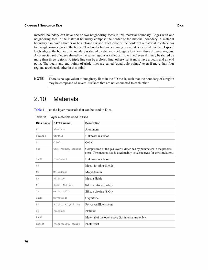
DIOSCHAPTER 2 SIMULATOR DIOS
material boundary can have one or two neighboring faces in this material boundary. Edges with oneneighboring face in the material boundary compose the border of the material boundary. A materialboundary can have a border or be a closed surface. Each edge of the border of a material interface hastwo neighboring edges in the border. The border has no beginning or end; it is a closed line in 3D space.Each edge in the border of a boundary is shared by elements belonging to at least three different regions.A connected set of edges shared by the same regions is called a ‘triple line,’ even if it may be shared bymore than three regions. A triple line can be a closed line, otherwise, it must have a begin and an endpoint. The begin and end points of triple lines are called ‘quadruple points,’ even if more than fourregions touch each other in this point.
NOTE There is no equivalent to imaginary lines in the 3D mesh, such that the boundary of a regionmay be composed of several surfaces that are not connected to each other.
2.10 MaterialsTable 11 lists the layer materials that can be used in Dios.
Table 11 Layer materials used in Dios
Dios name DATEX name Description
Al Aluminum Aluminum
Ceramic Ceramic Unknown insulator
Co Cobalt Cobalt
Gas Gas, Vacuum, Ambient Composition of the gas layer is described by parameters in the process steps. The material Gas is used mainly to select areas for the simulation.
IsoX InsulatorX Unknown insulator
Me Metal, forming silicide
Mo Molybdenum Molybdenum
MS Silicide Metal silicide
Ni Si3N4, Nitride Silicon nitride (Si3N4)
Ox Oxide, SiO2 Silicon dioxide (SiO2)
OxyN Oxynitride Oxynitride
Po PolySi, Polysilicon Polycrystalline silicon
Pt Platinum Platinum
Rand Material of the outer space (for internal use only)
Resist Photoresist, Resist Photoresist
70
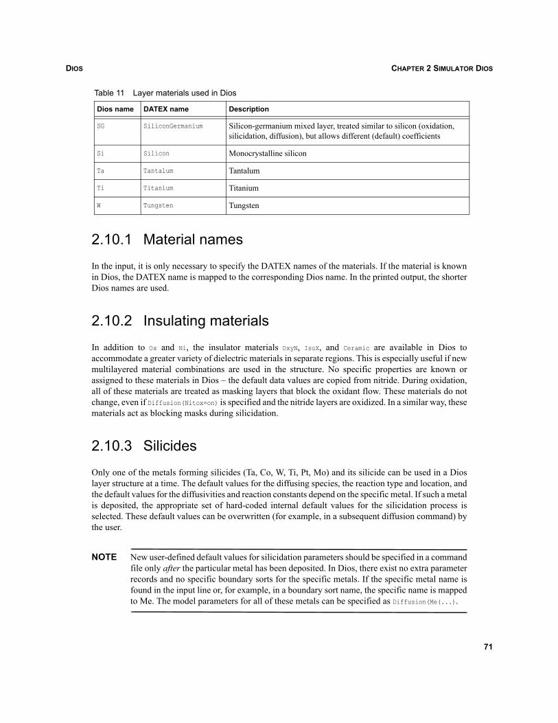
DIOS CHAPTER 2 SIMULATOR DIOS
2.10.1 Material names
In the input, it is only necessary to specify the DATEX names of the materials. If the material is knownin Dios, the DATEX name is mapped to the corresponding Dios name. In the printed output, the shorterDios names are used.
2.10.2 Insulating materials
In addition to Ox and Ni, the insulator materials OxyN, IsoX, and Ceramic are available in Dios toaccommodate a greater variety of dielectric materials in separate regions. This is especially useful if newmultilayered material combinations are used in the structure. No specific properties are known orassigned to these materials in Dios – the default data values are copied from nitride. During oxidation,all of these materials are treated as masking layers that block the oxidant flow. These materials do notchange, even if Diffusion(Nitox=on) is specified and the nitride layers are oxidized. In a similar way, thesematerials act as blocking masks during silicidation.
2.10.3 Silicides
Only one of the metals forming silicides (Ta, Co, W, Ti, Pt, Mo) and its silicide can be used in a Dioslayer structure at a time. The default values for the diffusing species, the reaction type and location, andthe default values for the diffusivities and reaction constants depend on the specific metal. If such a metalis deposited, the appropriate set of hard-coded internal default values for the silicidation process isselected. These default values can be overwritten (for example, in a subsequent diffusion command) bythe user.
NOTE New user-defined default values for silicidation parameters should be specified in a commandfile only after the particular metal has been deposited. In Dios, there exist no extra parameterrecords and no specific boundary sorts for the specific metals. If the specific metal name isfound in the input line or, for example, in a boundary sort name, the specific name is mappedto Me. The model parameters for all of these metals can be specified as Diffusion(Me(...).
SG SiliconGermanium Silicon-germanium mixed layer, treated similar to silicon (oxidation, silicidation, diffusion), but allows different (default) coefficients
Si Silicon Monocrystalline silicon
Ta Tantalum Tantalum
Ti Titanium Titanium
W Tungsten Tungsten
Table 11 Layer materials used in Dios
Dios name DATEX name Description
71
DIOSCHAPTER 2 SIMULATOR DIOS
2.10.4 Amorphous silicon
In Dios, amorphous silicon is not defined as a material. A large value of the dataset Amorphization isused to indicate amorphous regions in silicon. The threshold value can be specified asImplantation(Threshold=1.15e22). Amorphous regions are automatically defined during ion implantationand removed when the first accepted time step of the anneal following the implantation has beenaccepted. The user can modify the dataset Amorphization when loading analytic profiles with the Loadcommand. The dataset Amorphization is used mainly to define the initial profiles of silicon point defectsfor the point defect–assisted diffusion. There are no special diffusion, clustering, or trapping models foramorphous silicon in Dios except the special choice of the initial point defect concentrations.
2.10.5 Silicon germanium
The material SG has been defined formally as a copy of crystalline silicon (Si). This allows differentdefault values to be defined in the two crystalline silicon materials Si and SG as a very primitive versionof silicon germanium process simulation. The boundary between the Si and SG regions does not move.A more realistic simulation of silicon germanium can be performed using the simulation of deposition,or by the loading or implantation of a germanium profile into a silicon region. The germanium profilespreads during subsequent diffusions; an interdiffusion is always assumed and no sharp interfacesbetween silicon (Si with low Ge content) and silicon germanium (Si with high Ge content) are definedin Dios. In this case, there is no need to use the material SG at all. (The diffusion of a germanium profilein SG and the interaction at a silicon–silicon germanium interface is not forbidden, but it is notrecommended or tested.)
For each line in the 2D Dios layer system and in the 2D triangulation, a boundary sort is defined. Theboundary sort is used mainly to refer to models and parameters describing the behavior at the interfacebetween two adjacent materials. The name of the boundary sort is defined as the concatenation of thetwo Dios material names (SiOx). In the input, the user can also use the concatenation of the DATEXnames. The order of the material names in the concatenation is not important. If the boundary sort iswritten into the output, the name may deviate from the user input: the order of the materials may bechanged and always the Dios material names are used.
The special boundary sort (Imag) is used for the imaginary lines linking inclusions with the ‘main’ layersystem. The top, bottom, left, and right parts of the outer contour of the layer system are marked bydifferent boundary sorts (ORAND, URAND, LRAND, RRAND, RAND). The boundary sorts can bedisplayed in the Dios graphics by toggling the layer button in the graphics window several times or byspecifying Graphics(layer=sort,plot).
2.11 DatasetsThe unknown functions (also called variables, species, or datasets) are defined on the simulation grid.Most are defined as piecewise linear or piecewise logarithmic along the edges of the simulation grid. Foreach mesh point (precisely for each region sharing the mesh point), a value is known. The piecewiselinear or logarithmic functions can be discontinuous at the boundaries; inside of the areas, they arecontinuous. Independent surface values (for example, concentrations) are defined as piecewise linear
72
DIOS CHAPTER 2 SIMULATOR DIOS
functions along the boundaries. They can be defined only for some of the boundaries and can havediscontinuity in triple points.
Some of the functions are interpreted as constant per element. This can be, for example, stresscomponents or functions, used to accumulate data during the Monte Carlo ion implantation.
The functions on the grid are introduced or deleted during the simulation if necessary. The datasets inDios are grouped; several datasets can be associated to the same impurity species and just denotedifferent modifications containing the same kind of atoms. Total concentrations, for example, AsTotalare the major modifications of a impurity. The total concentrations are always defined if an impurityspecies is introduced in the simulation. During an ion implantation of arsenic, for example, either thetotal arsenic concentration is introduced newly or the existing concentration is modified.
Besides the total concentration of an impurity species, the substitutional (active) concentrations arealways defined, for example, AsActive. The clustering and diffusion models can be selected so that insome materials, or even everywhere on the simulation grid, the total and active concentrations of adopant are equal. The existence of datasets for the substitutional concentrations allows a more cleaninterface when saving data to the device simulator Sentaurus Device. Depending on the selecteddiffusion and clustering models, further modifications of the dopants are defined and introduced intoDios: clusters, pairs. These are usually removed automatically if the models are changed. Sometimes,even the total concentrations are removed in Dios, for example, if after a load or an etching step theentire dataset has only very low values.
The silicon self interstitials and vacancies are formally treated as dopant species similar to, for example,arsenic. The appropriate total concentrations (ITotal and VTotal) of the point defects are defined ormodified during the simulation of the ion implantation. The total point defect concentrations are crucialfor the transient point defect–assisted dopant diffusion; their initial concentration at the start of adiffusion step is very often modified to calibrate the diffused profiles. Besides the total concentration,the neutral, unpaired point defect concentrations (I0 and V0) are important to understand the transientbehavior and the transition to equilibrium diffusion. The neutral unpaired point defects are treatedsimilarly to the substitutional (active) concentrations of the dopant species. There exist furthermodifications of point defects – charged point defects, pairs of dopants and point defects, point defectclusters, and trapped point defects.
Since the initial total point defect concentrations are often modified to adjust the transient diffusionbehavior, the implantation damage is kept separate from the point defect concentrations. The damage isstored in the dataset Amorphization. This dataset is used solely to accumulate the damage oversubsequent implantations and to properly describe the formation of amorphized regions during the ionimplantation and to indicate these amorphized regions. It is not otherwise used: neither to indicate verysmall grains in polysilicon nor to define any initial damage for point defect–assisted diffusion.
Net doping, net active (NetActive) concentration, total doping, electron (NDensity) and hole (PDensity)concentrations, and electrostatic potential (U) are functions that are derived according to the selectedmodels from the dopant concentrations. They are always defined in Dios. The NetActive concentrationis defined in Dios as the signed sum of all substitutional concentrations (multiplied with the chargenumber). This is usually transferred to the device simulator (that is, saved for type=mdraw). The Netconcentration is defined in Dios as the signed sum of all charged species, for example, including chargedpoint defects and pairs, partially charged clusters and so on, depending on the diffusion and clustering
73
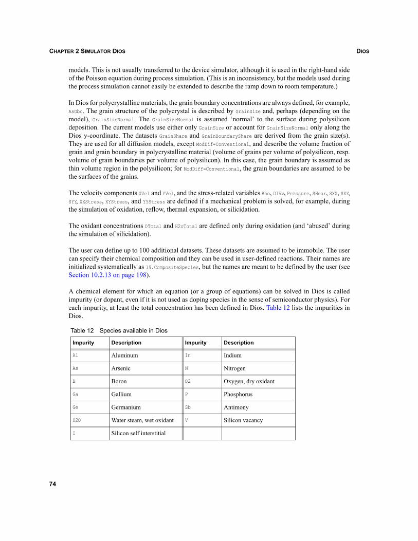
DIOSCHAPTER 2 SIMULATOR DIOS
models. This is not usually transferred to the device simulator, although it is used in the right-hand sideof the Poisson equation during process simulation. (This is an inconsistency, but the models used duringthe process simulation cannot easily be extended to describe the ramp down to room temperature.)
In Dios for polycrystalline materials, the grain boundary concentrations are always defined, for example,AsGbc. The grain structure of the polycrystal is described by GrainSize and, perhaps (depending on themodel), GrainSizeNormal. The GrainSizeNormal is assumed ‘normal’ to the surface during polysilicondeposition. The current models use either only GrainSize or account for GrainSizeNormal only along theDios y-coordinate. The datasets GrainShare and GrainBoundaryShare are derived from the grain size(s).They are used for all diffusion models, except ModDif=Conventional, and describe the volume fraction ofgrain and grain boundary in polycrystalline material (volume of grains per volume of polysilicon, resp.volume of grain boundaries per volume of polysilicon). In this case, the grain boundary is assumed asthin volume region in the polysilicon; for ModDiff=Conventional, the grain boundaries are assumed to bethe surfaces of the grains.
The velocity components XVel and YVel, and the stress-related variables Rho, DIVv, Pressure, SHear, SXX, SXY,SYY, XXStress, XYStress, and YYStress are defined if a mechanical problem is solved, for example, duringthe simulation of oxidation, reflow, thermal expansion, or silicidation.
The oxidant concentrations OTotal and H2oTotal are defined only during oxidation (and ‘abused’ duringthe simulation of silicidation).
The user can define up to 100 additional datasets. These datasets are assumed to be immobile. The usercan specify their chemical composition and they can be used in user-defined reactions. Their names areinitialized systematically as 19.CompositeSpecies, but the names are meant to be defined by the user (seeSection 10.2.13 on page 198).
A chemical element for which an equation (or a group of equations) can be solved in Dios is calledimpurity (or dopant, even if it is not used as doping species in the sense of semiconductor physics). Foreach impurity, at least the total concentration has been defined in Dios. Table 12 lists the impurities inDios.
Table 12 Species available in Dios
Impurity Description Impurity Description
Al Aluminum In Indium
As Arsenic N Nitrogen
B Boron O2 Oxygen, dry oxidant
Ga Gallium P Phosphorus
Ge Germanium Sb Antimony
H2O Water steam, wet oxidant V Silicon vacancy
I Silicon self interstitial
74

DIOS CHAPTER 2 SIMULATOR DIOS
Formally, all model parameters are defined for each impurity, each material, and each boundary sort.Sometimes, parameter declarations have been omitted in the command interpreter if the parameter is notmeaningful for the impurity, for example, if no model can be selected that would use this parameter.
Appendix A on page 315 lists all of the Dios datasets.
75

DIOSCHAPTER 2 SIMULATOR DIOS
76
DIOS CHAPTER 3 TITLE COMMAND
Dios
CHAPTER 3 Title command
The Title command is the first command in a Dios simulation. Several simulations can be grouped inone command file if they are encapsulated by a Title statement at the start and a Reset command at theend. The Reset statement is necessary because Title does not, in general, reset all of the simulationparameters and datasets. Appendix B on page 327 lists the Title command parameters.
3.1 MAXVThe maximum number of mesh points MAXV can be specified in the Title command. This number restrictsthe number of points during the mesh adaptation; it does not restrict the number inserted in thepostprocessing (delaunization). By default, no limit on MAXV is defined, that is, the program automaticallyreallocates memory if this is required during the generation or modification of the mesh. All datasets andother mesh size–dependent data are reallocated and the mesh adaptation is restarted. If an upper limit ofMAXV is prescribed and if the refined mesh will contain more than MAXV mesh points, the last validtriangulation is restored and further refinement is cancelled. The restriction of the number of nodes inthe grid can be useful on machines with small main memory resources or to avoid some repetition ofadaptation by allocating initially a sufficiently large number of mesh points.
NOTE It is generally not recommended to specify any other MAX* parameter. They are all chosenaccording to MAXV and should be specified only in special cases if advised by the SynopsysTechnical Support Center.
3.2 NewDiffIt is recommended to select the desired grid strategy at this initial stage in the simulation. Unlessotherwise specified, Dios assumes NewDiff=1, which means that a mesh is produced in all layers togetherwith an evaluation of simulated variables in all layers.
77
DIOSCHAPTER 3 TITLE COMMAND
3.3 SiDiffIt is also recommended to specify the diffusion strategy at this stage. If not specified, Dios runs withSiDiff=on and diffusion is only simulated in the silicon substrate. No diffusion is simulated in depositedlayers such as polysilicon and oxide. If several simulations are controlled by the same command file, usethe Reset command (see Section 2.6 on page 65).
NOTE In the Reset command, the layer structure, mesh, and datasets are deleted, and the entirecommand interpreter is reset to its initial internal default state. No modification of defaultvalues or definition of species, names, and so on will endure.
78
DIOS CHAPTER 4 GRID COMMAND
Dios
CHAPTER 4 Grid command
4.1 OverviewAll three grid types – USER, ITRI, and UTRI – have their own internal data structure on memory. The USERand ITRI grids are of internal and technical relevance, and useful to describe or explain the appliedalgorithms. The UTRI grid is the central data structure for the simulation of diffusion and mechanicsequations, for the representation of datasets, and for the simulation of Monte Carlo ion implantation withCrystal-TRIM. Appendix C on page 329 lists the Grid command parameters.
In the Grid command, various types of initial grid construction algorithms can be selected. Therefinement process is controlled mainly by the parameters in the Control parameter record. Theseparameters are described in Section Q.2 on page 554. The postprocessing and delaunization algorithmscan be controlled (for example, restricted) only to a certain degree since in Dios, for example, thesimulation of diffusion relies on a certain mesh quality. Wherever possible, this mesh quality is enforcedin Dios, that is, a boundary-conforming Delaunay mesh is constructed.
Dios does not provide a mesh coarsening algorithm. Whenever the doping profiles or geometry havechanged significantly, the mesh adaptation always builds a completely new mesh. This requires therepetition of all steps in Section 4.2 on page 80 and is usually performed only after a series of time stepsof diffusion, during the simulation of ion implantation, and when loading external profiles. By default,at the start of each mesh adaptation, a new USER grid is built.
The local adaption to the current layer structure is repeated whenever an up-to-date grid is required aftera modification of the layer structure. To save time, this is performed only at the end of the ‘cold’structuring operations (etching, deposition, mask generation, and CMP), but the adaptation is requiredat the end of each time step of a ‘hot’ change of the layer structure in oxidation, epitaxy, silicidation,glass reflow, or thermal expansion calculation. Adapting the grid to the new layer structure requiresrepetition of at least steps 4 to 7 in Section 4.2.
If the layer structure is modified significantly by adding a thick layer (for example, a mask) on top ofthe structure, the USER grid must be expanded to the top and the entire mesh refinement and adaptationmust be repeated. Although this is allowed, there is no need (and it is also not recommended) to repeatthe Grid command. Dios deals with this automatically.
At the beginning of the layer system operations (mask, deposit) and during diffusion steps (oxidationand especially epitaxy), the structure is checked to see if the USER grid will still contain the expected finalstructure. If necessary, the USER grid is expanded, and the entire refinement and adaptation procedure isrepeated. Before generating the new USER grid, the program checks automatically if the top grid line ofthe new triangulation will be above the topmost (non-gas) point in the layer system plus an additionalsafety spacing: Control(SafetyGrid=0.4). If necessary, the USER grid is expanded at the top by adding moreelements. This expansion is performed for all meshing modes (even for NewDiff=0). Otherwise, forexample, in the case of an epitaxy, the mesh quality would deteriorate significantly.
79
DIOSCHAPTER 4 GRID COMMAND
The edges on the outer boundary of the USER grid are labeled with a number (by default, +1 for the left,right, and bottom parts, and +2 on the top line). These numbers are always defined, but are used only forNewDiff=0 to encode the boundary conditions. They are also used when manipulating USER grids (seeSection 4.3.2 on page 84).
4.2 Constructing simulation gridThe simulation grid in Dios is ‘constructed’ in several steps:
1. A first coarse triangulation is constructed from scratch, covering the entire simulation domain (butnot resolving any gradients or material interfaces). This is called initial or USER grid.
2. A refinement triangle tree is built by subsequent splitting of the triangles. This tree is called ITRIgrid.
3. The leaf elements of the refinement tree are extracted.
4. The grid is adapted to the layer structure. Two strategies for this adaptation have been implementedin Dios. The applied method is selected by the parameter NewDiff. It can be changed during the flowof the simulation. The vertical transformation applied for NewDiff=0 is described in Section 4.4.1 onpage 90 and the subdivision of the mesh that is selected with NewDiff=1 is described in Section 4.4.2on page 91. The result of either method to adapt the grid to the layer structure is called UTRI grid. Inthe UTRI grid, each triangle is assigned to just one material and region (area), and the materialboundaries (lines) of the layer structure are approximated by corresponding boundaries in thetriangulation.
5. The mesh points on the left side of the grid are extracted, and a special 1D mesh is constructed (onlyfor 1D layer structure, 1D data profiles, and only if Control(1D=on) (default)).
6. Postprocessing, mesh optimization (surface-parallel refinement, mesh smoothing, delaunization).
7. All datasets are reinterpolated (sometimes including specific definition from external data).
4.3 User gridFor each vertex of the user grid, the coordinates GX and GY and, for each triangle, the three (global) vertexnumbers (ITNODE) and the triangle type (ITYPET) are stored. In addition, boundary information for theedges adjacent to the vertices is stored (ITEDGE). Neither refinement nor layer structure is described inthis data structure. Although this is not necessary, the extensions of the user grid usually coincide withthe bounding box, containing the layer structure (including the gas).
Different types of user triangulation can be used in Dios. The meshes for TYPe=Default can be specifiedby either of the following commands:
GRID(X=(x1=.,x2=.),Y=(y1=.,y2=.),NX=.)GRID(X=(x1=.,x2=.),Y=(y1=.,y2=.),DX=.)
80
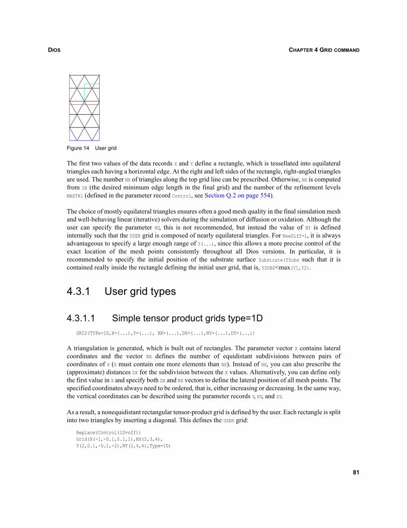
DIOS CHAPTER 4 GRID COMMAND
Figure 14 User grid
The first two values of the data records X and Y define a rectangle, which is tessellated into equilateraltriangles each having a horizontal edge. At the right and left sides of the rectangle, right-angled trianglesare used. The number NX of triangles along the top grid line can be prescribed. Otherwise, NX is computedfrom DX (the desired minimum edge length in the final grid) and the number of the refinement levelsMAXTRl (defined in the parameter record Control, see Section Q.2 on page 554).
The choice of mostly equilateral triangles ensures often a good mesh quality in the final simulation meshand well-behaving linear (iterative) solvers during the simulation of diffusion or oxidation. Although theuser can specify the parameter NY, this is not recommended, but instead the value of NY is definedinternally such that the USER grid is composed of nearly equilateral triangles. For NewDiff=1, it is alwaysadvantageous to specify a large enough range of Y(...), since this allows a more precise control of theexact location of the mesh points consistently throughout all Dios versions. In particular, it isrecommended to specify the initial position of the substrate surface Substrate(YSubs such that it iscontained really inside the rectangle defining the initial user grid, that is, YSUBS<max(Y1,Y2).
4.3.1 User grid types
4.3.1.1 Simple tensor product grids type=1DGRID(TYPe=1D,X=(...),Y=(...), NX=(...),DX=(...),NY=(...),DY=(...))
A triangulation is generated, which is built out of rectangles. The parameter vector X contains lateralcoordinates and the vector NX defines the number of equidistant subdivisions between pairs ofcoordinates of X (X must contain one more elements than NX). Instead of NX, you can also prescribe the(approximate) distances DX for the subdivision between the X values. Alternatively, you can define onlythe first value in X and specify both DX and NX vectors to define the lateral position of all mesh points. Thespecified coordinates always need to be ordered, that is, either increasing or decreasing. In the same way,the vertical coordinates can be described using the parameter records Y, NY, and DY.
As a result, a nonequidistant rectangular tensor-product grid is defined by the user. Each rectangle is splitinto two triangles by inserting a diagonal. This defines the USER grid:
Replace(Control(1D=off))Grid(X(-1,-0.1,0.1,1),NX(2,3,4),Y(2,0.1,-0.1,-2),NY(2,4,4),Type=1D)
81
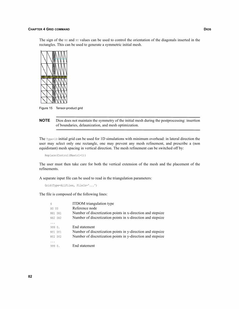
DIOSCHAPTER 4 GRID COMMAND
The sign of the NX and NY values can be used to control the orientation of the diagonals inserted in therectangles. This can be used to generate a symmetric initial mesh.
Figure 15 Tensor-product grid
NOTE Dios does not maintain the symmetry of the initial mesh during the postprocessing: insertionof boundaries, delaunization, and mesh optimization.
The Type=1D initial grid can be used for 1D simulations with minimum overhead: in lateral direction theuser may select only one rectangle, one may prevent any mesh refinement, and prescribe a (nonequidistant) mesh spacing in vertical direction. The mesh refinement can be switched off by:
Replace(Control(Maxtrl=1))
The user must then take care for both the vertical extension of the mesh and the placement of therefinements.
A separate input file can be used to read in the triangulation parameters:
Grid(Type=AllFiles, FileIn='...')
The file is composed of the following lines:
6 ITDOM triangulation typeX0 Y0 Reference nodeNX1 DX1 Number of discretization points in x-direction and stepsizeNX2 DX2 Number of discretization points in x-direction and stepsize...
999 0. End statementNY1 DY1 Number of discretization points in y-direction and stepsizeNY2 DY2 Number of discretization points in y-direction and stepsize...
999 0. End statement
82
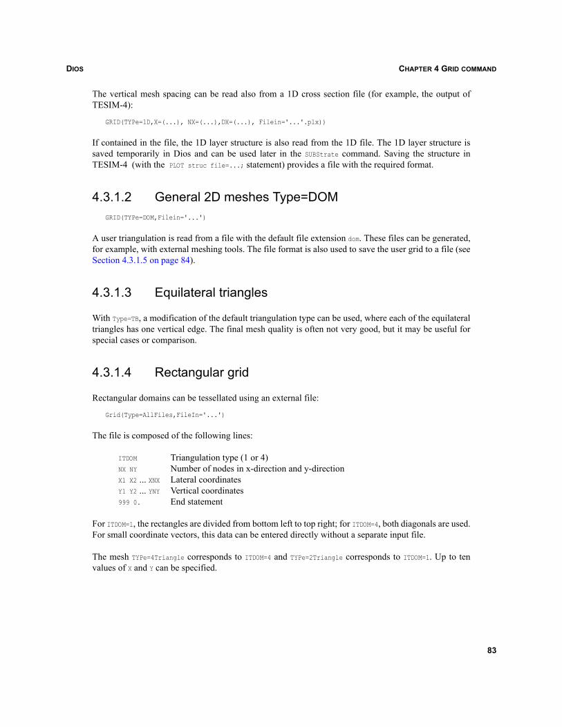
DIOS CHAPTER 4 GRID COMMAND
The vertical mesh spacing can be read also from a 1D cross section file (for example, the output ofTESIM-4):
GRID(TYPe=1D,X=(...), NX=(...),DX=(...), Filein='...'.plx))
If contained in the file, the 1D layer structure is also read from the 1D file. The 1D layer structure issaved temporarily in Dios and can be used later in the SUBStrate command. Saving the structure inTESIM-4 (with the PLOT struc file=...; statement) provides a file with the required format.
4.3.1.2 General 2D meshes Type=DOMGRID(TYPe=DOM,Filein='...')
A user triangulation is read from a file with the default file extension dom. These files can be generated,for example, with external meshing tools. The file format is also used to save the user grid to a file (seeSection 4.3.1.5 on page 84).
4.3.1.3 Equilateral triangles
With Type=TB, a modification of the default triangulation type can be used, where each of the equilateraltriangles has one vertical edge. The final mesh quality is often not very good, but it may be useful forspecial cases or comparison.
4.3.1.4 Rectangular grid
Rectangular domains can be tessellated using an external file:
Grid(Type=AllFiles,FileIn='...')
The file is composed of the following lines:
ITDOM Triangulation type (1 or 4)NX NY Number of nodes in x-direction and y-directionX1 X2 ... XNX Lateral coordinatesY1 Y2 ... YNY Vertical coordinates999 0. End statement
For ITDOM=1, the rectangles are divided from bottom left to top right; for ITDOM=4, both diagonals are used.For small coordinate vectors, this data can be entered directly without a separate input file.
The mesh TYPe=4Triangle corresponds to ITDOM=4 and TYPe=2Triangle corresponds to ITDOM=1. Up to tenvalues of X and Y can be specified.
83
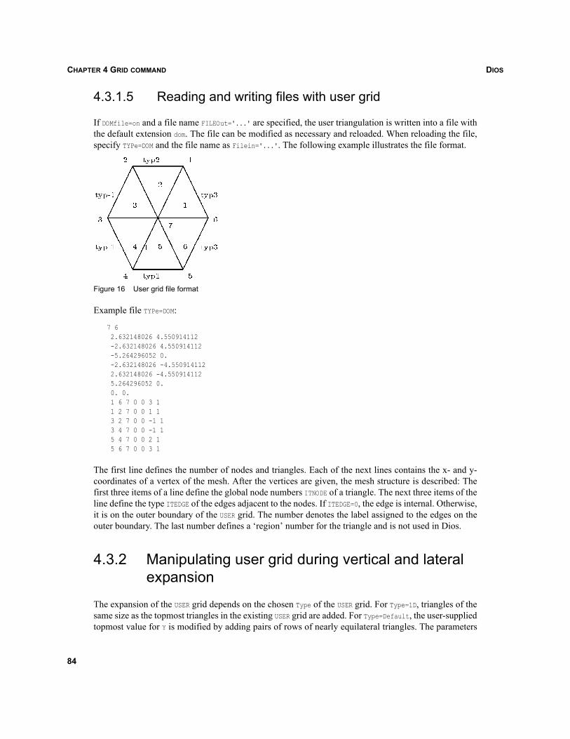
DIOSCHAPTER 4 GRID COMMAND
4.3.1.5 Reading and writing files with user grid
If DOMfile=on and a file name FILEOut='...' are specified, the user triangulation is written into a file withthe default extension dom. The file can be modified as necessary and reloaded. When reloading the file,specify TYPe=DOM and the file name as Filein='...'. The following example illustrates the file format.
Figure 16 User grid file format
Example file TYPe=DOM:
7 6 2.632148026 4.550914112 -2.632148026 4.550914112 -5.264296052 0. -2.632148026 -4.550914112 2.632148026 -4.550914112 5.264296052 0. 0. 0. 1 6 7 0 0 3 1 1 2 7 0 0 1 1 3 2 7 0 0 -1 1 3 4 7 0 0 -1 1 5 4 7 0 0 2 1 5 6 7 0 0 3 1
The first line defines the number of nodes and triangles. Each of the next lines contains the x- and y-coordinates of a vertex of the mesh. After the vertices are given, the mesh structure is described: Thefirst three items of a line define the global node numbers ITNODE of a triangle. The next three items of theline define the type ITEDGE of the edges adjacent to the nodes. If ITEDGE=0, the edge is internal. Otherwise,it is on the outer boundary of the USER grid. The number denotes the label assigned to the edges on theouter boundary. The last number defines a ‘region’ number for the triangle and is not used in Dios.
4.3.2 Manipulating user grid during vertical and lateral expansion
The expansion of the USER grid depends on the chosen Type of the USER grid. For Type=1D, triangles of thesame size as the topmost triangles in the existing USER grid are added. For Type=Default, the user-suppliedtopmost value for Y is modified by adding pairs of rows of nearly equilateral triangles. The parameters
84
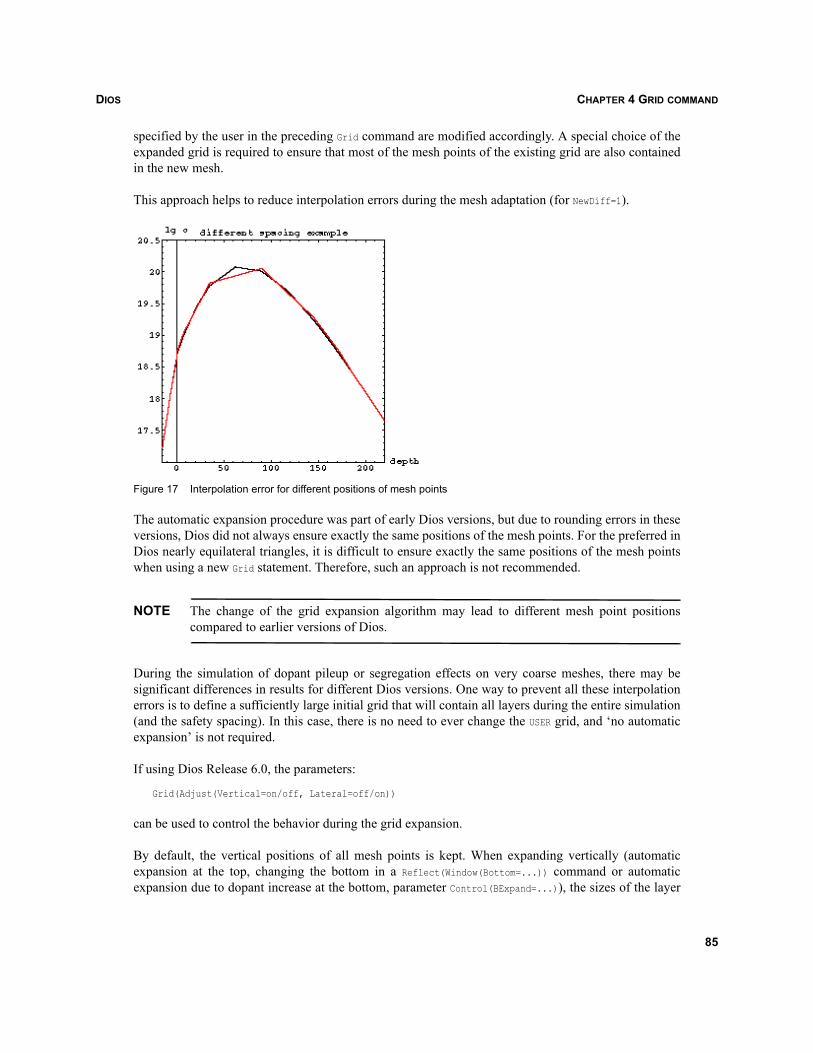
DIOS CHAPTER 4 GRID COMMAND
specified by the user in the preceding Grid command are modified accordingly. A special choice of theexpanded grid is required to ensure that most of the mesh points of the existing grid are also containedin the new mesh.
This approach helps to reduce interpolation errors during the mesh adaptation (for NewDiff=1).
Figure 17 Interpolation error for different positions of mesh points
The automatic expansion procedure was part of early Dios versions, but due to rounding errors in theseversions, Dios did not always ensure exactly the same positions of the mesh points. For the preferred inDios nearly equilateral triangles, it is difficult to ensure exactly the same positions of the mesh pointswhen using a new Grid statement. Therefore, such an approach is not recommended.
NOTE The change of the grid expansion algorithm may lead to different mesh point positionscompared to earlier versions of Dios.
During the simulation of dopant pileup or segregation effects on very coarse meshes, there may besignificant differences in results for different Dios versions. One way to prevent all these interpolationerrors is to define a sufficiently large initial grid that will contain all layers during the entire simulation(and the safety spacing). In this case, there is no need to ever change the USER grid, and ‘no automaticexpansion’ is not required.
If using Dios Release 6.0, the parameters:
Grid(Adjust(Vertical=on/off, Lateral=off/on))
can be used to control the behavior during the grid expansion.
By default, the vertical positions of all mesh points is kept. When expanding vertically (automaticexpansion at the top, changing the bottom in a Reflect(Window(Bottom=...)) command or automaticexpansion due to dopant increase at the bottom, parameter Control(BExpand=...)), the sizes of the layer
85
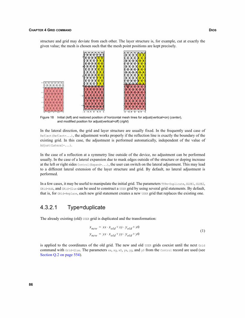
DIOSCHAPTER 4 GRID COMMAND
structure and grid may deviate from each other. The layer structure is, for example, cut at exactly thegiven value; the mesh is chosen such that the mesh point positions are kept precisely.
Figure 18 Initial (left) and restored position of horizontal mesh lines for adjust(vertical=on) (center), and modified position for adjust(vertical=off) (right)
In the lateral direction, the grid and layer structure are usually fixed. In the frequently used case ofReflect(Reflect=...), the adjustment works properly if the reflection line is exactly the boundary of theexisting grid. In this case, the adjustment is performed automatically, independent of the value ofAdjust(Lateral=...).
In the case of a reflection at a symmetry line outside of the device, no adjustment can be performedusually. In the case of a lateral expansion due to mask edges outside of the structure or doping increaseat the left or right sides Control(Expand=...), the user can switch on the lateral adjustment. This may leadto a different lateral extension of the layer structure and grid. By default, no lateral adjustment isperformed.
In a few cases, it may be useful to manipulate the initial grid. The parameters TYPe=Duplicate, GLUE1, GLUE2,GRid=Add, and GRid=Glue can be used to construct a USER grid by using several grid statements. By default,that is, for GRid=Replace, each new grid statement creates a new USER grid that replaces the existing one.
4.3.2.1 Type=duplicate
The already existing (old) USER grid is duplicated and the transformation:
(1)
is applied to the coordinates of the old grid. The new and old USER grids coexist until the next Gridcommand with Grid=Glue. The parameters xx, xy, x0, yx, yy, and y0 from the Control record are used (seeSection Q.2 on page 554).
xnew xx xold⋅ xy yold⋅ x0+ +=
ynew yx xold⋅ yy yold⋅ y0+ +=
86
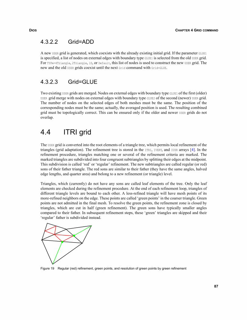
DIOS CHAPTER 4 GRID COMMAND
4.3.2.2 Grid=ADD
A new USER grid is generated, which coexists with the already existing initial grid. If the parameter GLUE1is specified, a list of nodes on external edges with boundary type GLUE1 is selected from the old USER grid.For TYPe=4Triangle, 2Triangle, 1D, or Default, this list of nodes is used to construct the new USER grid. Thenew and the old USER grids coexist until the next Grid command with Grid=GLUE.
4.3.2.3 Grid=GLUE
Two existing USER grids are merged. Nodes on external edges with boundary type GLUE1 of the first (older)USER grid merge with nodes on external edges with boundary type GLUE2 of the second (newer) USER grid.The number of nodes on the selected edges of both meshes must be the same. The position of thecorresponding nodes must be the same; actually, the averaged position is used. The resulting combinedgrid must be topologically correct. This can be ensured only if the older and newer USER grids do notoverlap.
4.4 ITRI gridThe USER grid is converted into the root elements of a triangle tree, which permits local refinement of thetriangles (grid adaptation). The refinement tree is stored in the ITRI, IVERT, and IUSR arrays [4]. In therefinement procedure, triangles matching one or several of the refinement criteria are marked. Themarked triangles are subdivided into four congruent subtriangles by splitting their edges at the midpoint.This subdivision is called ‘red’ or ‘regular’ refinement. The new subtriangles are called regular (or red)sons of their father triangle. The red sons are similar to their father (they have the same angles, halvededge lengths, and quarter area) and belong to a new refinement (or triangle) level.
Triangles, which (currently) do not have any sons are called leaf elements of the tree. Only the leafelements are checked during the refinement procedure. At the end of each refinement loop, triangles ofdifferent triangle levels are bound to each other. A less-refined triangle will have mesh points of itsmore-refined neighbors on the edge. These points are called ‘green points’ in the coarser triangle. Greenpoints are not admitted in the final mesh. To resolve the green points, the refinement zone is closed bytriangles, which are cut in half (green refinement). The green sons have typically smaller anglescompared to their father. In subsequent refinement steps, these ‘green’ triangles are skipped and their‘regular’ father is subdivided instead.
Figure 19 Regular (red) refinement, green points, and resolution of green points by green refinement
87
DIOSCHAPTER 4 GRID COMMAND
The refinement parameters are contained in the data record Control. They can be changed globally withthe Replace command or locally for a single process step. The following refinement criteria are used.
RefineGradient
Refines triangles with steep doping gradients. The ‘gradient’ of a function u in each triangle is definedby:
(2)
For each function, the value IVER (in percent) can be defined as:
Replace(Control(IVer(AsTotal=...)
If for one of the functions in a triangle, the ‘gradient’ is larger than the specified positive value IVER, andif the triangle is allowed to be refined (that is, it is still ‘large’ enough), it is refined. If the value of IVERfor a dataset is set to zero, this dataset is no longer checked during the evaluation of the gradientrefinement.
With Replace(Control(Mass=6), users can select another formula for computing the ‘gradient’:
(3)
The parameter Ashdiff can be specified also in the Control record. It is shared by all datasets. In Eq. 3,the function asinh() denotes the ‘transformed’ function. It is controlled by the parameter LogSwitch,which can be specified for each of the datasets Replace(Variable(Species=AsTotal, LogSwitch=0|1|2)) or asGraphic(LogSwitch(AsTotal=Linear|Flog|Asinh)):
RefineBoundary Refines triangles at material interfaces.
RefineJunction Refines triangles at p-n junctions.
RefineACInterface Refines triangles at amorphous-crystalline interfaces.
RefineBeforeFront Refines triangles in front of steep doping fronts.
RefineAll Refines triangles in user-defined rectangles.
RefinePoints Refines triangles at user-defined points.
RefineMaximum Refines triangles at a local dopant maxima.
RefineAll Refines all triangles.
RefineCurvature Refines triangles at changes of the sign of the curvature of a doping profile.
If one of the parameters is set to zero, the corresponding criterion is switched off.
ulog( )grad maxi jui uj–
ui uj+---------------------⎝ ⎠
⎛ ⎞ IVER 100.⁄>≈
maxijui( )asinh uj( )asinh–Ashdiff
----------------------------------------------------⎝ ⎠⎛ ⎞ IVER 100.⁄>
88
DIOS CHAPTER 4 GRID COMMAND
For a positive parameter value, the appropriate criterion is applied as many times as the value prescribes(independent of the triangle size). For RefineJunction=2, two refinement loops are performed and, in eachloop, all triangles with a p-n junction are refined.
NOTE The resulting mesh resolution in the vicinity of the junction may show a large variation,depending on the other refinement criteria.
For negative parameter values, the refinement criterion is applied only to ‘sufficiently large’ triangles.In this case, the absolute value of the parameter selects the refinement levels for each criterion. Onlytriangles with a refinement level below the absolute value are checked and may be refined. ForRefineJunction=-5, all triangles on refinement levels 1…4, which contain a p-n junction are refined. Asa result, all triangles containing p-n junctions are at level 5. This approach gives relative good controlover the size of the final grid elements.
The entire refinement process is organized in two subsequent refinement loops. In the first refinementloop, only the criteria with negative parameter values are selected: RefineGradient, RefineAll,RefineBoundary, RefineJunction, RefineACInterface, RefineCurvature, RefinePoints, and RefineMaximum arehandled. During this refinement loop, the number of refinements of a user triangle (that is, the trianglelevel) is restricted. The parameter MAXTRL defines a global maximum refinement level for all criteria:
Replace(Control(MAXTRl=5))
The MAXTRl value restricts the maximum triangle level for all refinement criteria with negative parametervalues: MAXTRl=5,RefineBoundary=-8 is equivalent to MAXTRl=5,RefineBoundary=-5.
In this refinement loop, only sufficiently large triangles are refined. All refinement criteria are checkedand the triangles that fulfill one of the criteria are marked. If all criteria have been checked, the markedtriangles are subdivided. The first refinement loop is finished when no triangles are marked any more.
In the second refinement loop, all of the parameters RefineGradient, RefineAll, RefineBoundary,RefineJunction, RefineACInterface, RefineCurvature, RefinePoints, and RefineMaximum with positive valuesare handled. The triangle level (and therefore the size of the triangles) is no longer checked during thisrefinement loop. An additional refinement is performed, regardless of how small or big the triangles arethat meet the criterion. The default values of the parameters RefineJunction and RefineACInterface are +2,and the default value for RefinePoints is +3.
The control parameters for all refinement criteria can be specified per material:
Replace(Control(Si(Maxtrl=6, RefineGradient=-6),Po(MaxTrl=3))
For each boundary sort, the refinement parameter RefineBoundary can be used to control the refinementof the mesh at all boundaries of that boundary sort:
Replace(Control(SiOx(RefineBoundary=9))
89
DIOSCHAPTER 4 GRID COMMAND
The user can also define up to 20 refinement rectangles together with the set of refinement parametersMaxtrl, RefineAll, RefineGradient, RefineBoundary, RefineCurvature, RefineJunction, RefineACInterface,RefineBeforeFront, and RefineMaximum, which is applied inside of the rectangle:
Replace(Control(Maxtrl=4Rec1(RefineAll=-3,XLeft=-1.,XRight=1um,YBottom=100nm, YTop=1um,MAXTRl=3)REC2(RefineAll=-4,XLeft=-2.,XRight=2um,YBottom=300nm,YTop=1um)))
For the NewDiff=0 meshing mode, the user can also specify for each rectangle which coordinate type tocheck: Icosw=Geometrical or Physical (see Section 4.4.1 on page 90).
Grid adaptation is performed automatically during ion implantation and if an external doping profile isloaded. During the high temperature steps, after each CHsteps time step, the grid is checked as to whichtriangles are now refined. Only sufficiently large triangles (that allow for further refinement) arechecked. If too many of the checked triangles are found to allow refinement (more than IVERADA inpercent), or if the geometry of the device has changed such that it would no longer fit into the usertriangulation, or if a p-n junction or a material boundary is found in a large triangle, the entire meshadaptation is repeated, starting from a new USER grid.
The parameters MIsteps and MAsteps can be used to control the minimum and maximum number of timesteps with no mesh readaptation in-between. A mesh readaptation can be enforced explicitly with theGrid and Adaptation commands (independent of the MIsteps and MAsteps values). By default, the mesh isadapted at the end of Mask, Deposit, and Etch commands. This is controlled by the parameterAdaptation=on/off in each of these commands. The adaptation at the end of the process step allows forrefinement of the grid in the vicinity of the new material interfaces.
In order for users to familiarize themselves with the adaptation mechanism and to understand the workand interaction of the refinement criteria and algorithm, it may be useful to run a few special simulationswith different refinement parameters and with the following setup:
Replace(Control(IpGrid=4))Graphic(Wait=0)Adapt()
With this setup, the grid is displayed after each refinement loop, and the criteria that caused refinementare indicated. Increasing values of IpGrid=1...4 can be used to enable the display of more intermediateand the final fabrication stages of the mesh.
4.4.1 Adapting grid to layer system: Vertical transformation
The refinement tree, although it is refined in the vicinity of the material interfaces, does not fit exactlythe layer structure. The adaptation to the layer structure is achieved in the next mesh fabrication stepafter the refinement tree has been constructed. Two different strategies can be used in Dios. The strategydescribed here was the default in versions prior to Release 6.0. The user can still select this with:
Replace(Control(NewDiff=0))
90
DIOS CHAPTER 4 GRID COMMAND
This ‘old’ strategy is still kept for some time to ensure compatibility with old projects. Except for bugfixes, it is no longer supported. Try to avoid using the NewDiff=0 mode in your new projects.
If the silicon substrate is only slightly nonplanar and if all unknowns are required only in the siliconsubstrate, a vertical transformation can be applied to all grid points with:
(4)
The bottom line of the triangulation remains fixed and the top grid line is mapped locally to match thesubstrate surface. The original coordinates of the mesh points, as they are defined in the USER grid, aresaved for subsequent transformation steps. These original coordinates are called geometricalcoordinates.
The coordinates of the mesh points after the transformation are called physical coordinates, which areused in the simulation. After this vertical grid transformation, all triangles and all grid points belong tothe silicon substrate. During oxidation or epitaxy simulation, the transformation is applied at each timestep. In the simulation of deposition, mask, or etching processes, it is applied only once at the end of theprocess. SOI-type structures cannot be simulated with this meshing mode, unless the entire insulatingoxide and the bulk silicon are removed from the simulation domain and replaced by a boundarycondition.
In addition, the vertical transformation method is inappropriate if the substrate surface becomes stronglynonplanar (etched substrates, trench structures, steep oxide contours). In this case, triangles may turnand overlap each other. To reduce and, if possible, eliminate such problems with the NewDiff=0 meshingapproach, after each vertical grid transformation step, the grid is checked to see if some triangles areturned. To restore a valid triangulation, a smoothing operation is applied to the turned triangles. Eachvertex of these turned triangles is moved into the center of mass of the surrounding triangles (or edges).
If this approach does not succeed in restoring a valid triangulation, neighboring triangles are smoothedalso. If this fails as well, the fit to the boundary is relaxed: grid points on the top surface of the grid maybe moved away from the surface. If all these operations cannot reconstruct a valid triangulation, as a lastpossibility, a global smoothing step on the entire mesh is tried and vertical stripes of the grid are nolonger transformed. A warning is given to the user. For these geometries, it is recommended to use thealternative meshing strategy that is available in Dios with the selection NewDiff=1 and described inSection 4.4.2.
4.4.2 Adapting grid to layer system: Triangle subdivision at interfaces
For strongly nonplanar substrate surfaces or if the grid is required in other than just the substrate region,a local transformation of the triangles at the material interfaces is performed. This mode can be selectedwith:
Replace(Control(NewDiff=1)) or Replace(Control(SiDiff=on))
xi,gi( ) xi,yi( )→
yi giysubs xi( ) gmax xi( )–( )
gmax xi( ) gmin–( )---------------------------------------------------------- gi gmin–( )+=
91
DIOSCHAPTER 4 GRID COMMAND
At the end of the refinement process, all leaf triangles from the triangle tree are selected and convertedinto a flat element list, containing vertex and neighborhood information. This grid is then intersectedwith the boundaries of the layer system, which is given by the set of polygons (see Section 2.9 onpage 69). To obtain an approximation of the boundaries in the grid, triangles are cut in the intersectionpoints and sometimes mesh points are moved.
In general, the new point is inserted where the boundary intersects a triangle edge. Sometimes, this leadsto extremely thin and eccentric elements (which may cause convergence problems later). Theparameters R1max, R2max, T1max, T2max, and Omax (in the data record Control) are used to solve these cases.These parameters are maximum values of barycentric (that is, local in a triangle) coordinates. If thebarycentric coordinates of the intersection point exceed a critical parameter, an exception handling isstarted and one of the mesh points is moved (it is too close to the intersection point). If all theseparameters are set =1, no exception handling is performed. The smaller the values, the more precise isthe representation of the layer structure, but more eccentric elements may be created.
The intersection lines, representing the material interfaces, are added into the list of triangles. Meshpoints at boundaries are duplicated (several times) to store the limit values of the functions from alladjacent regions and independent surface values on the adjacent boundaries. The mixed triangle and linesegment list is called a UTRI grid. The topology of the mesh is stored as a complex. The boundaries in thiscomplex have no points, since these are given by the mesh points (see Section 2.8 on page 67).
The described meshing algorithm is enabled for NewDiff=1. It is used for both values of SiDiff. ForSiDiff=on, dopant diffusion is computed only in the substrate. For SiDiff=off, the dopant diffusion iscomputed in all layers.
4.4.3 Forcing an adaptation step
The command Adaptation is used to force a readaptation of the grid. This should not be necessary in mostsituations. Mesh adaptation is performed during ion implantation, when loading a profile, whenspecifying a new grid, and during anneal steps, since the program checks automatically if a readaptationis necessary. It can be useful if the refinement parameters in the Control data record have been changed.Section Q.2 on page 554 lists the parameters of the record Control that can be specified in the Adaptationcommand.
4.4.4 One-dimensional mesh extraction
Usually, at the beginning of a process simulation, the layer structure and doping profiles are 1D for someprocess steps. For these structures in Dios, a triangle mesh can be used, which has only two vertical gridlines, but is fully adaptive in vertical direction. Dios does not contain a special 1D grid adaptionalgorithm.
The 1D adaptive grid is extracted by default at the end of the adaptation as long as the structure anddoping profiles remain 1D. The usual 2D grid adaptation algorithm described in the preceding sectionis used. In order to reduce the effort, the USER grid is constructed in a special way if Type=Default wasselected: As long as Dios is in 1D mode, the USER grid is restricted in the lateral direction such that,
92
DIOS CHAPTER 4 GRID COMMAND
starting at the specified value of XLEFT, only one (vertical) stripe of equilateral triangles is defined. (Alocal value of NX=1 and an appropriately adjusted local value of XRIGHT are used temporarily.)
In the log file, the used values of XLEFT and XRIGHT are indicated. This ensures the same quality of trianglesas if the full 2D USER grid was used. In particular, the same vertical positions of the mesh points at XLEFTare defined. The 1D grid is constructed from the final mesh after the mesh adaptation and the adjustmentto the layer structure by extracting the vertical position of all nodes at the left side of the grid at XLEFT.These mesh points are duplicated at the right side of the device geometry, that is, at the original positionof XRIGHT as it was defined by the user in the Grid command. The final mesh is constructed in the sameway as the USER grid for Type=1D.
The resulting 1D mesh contains significantly less points than the 2D grid because of the elimination ofall mesh points sharing the same vertical coordinate but having different lateral coordinates. The verticalposition of all points is exactly the same as in the 2D mesh and, therefore, the diffusion simulation (andthe discretization errors) must be identical. One-dimensional profiles computed with the 1D extractedmesh and the 2D mesh as defined by the user should be identical. The 1D grid extraction algorithm isenabled by default: Replace(Control(1D=undefined)). The adaptive 1D mesh is used only as long as a 1Dsituation is given. When the first mask corner is encountered in the simulation domain or when a 2Ddoping profile is loaded, the grid switches to the usual 2D mode.
NOTE For 1D=on, a 1D mesh is always used even if a mask was created inside of the domain.
In the 1D mode, besides the grid, the layer description is forced to remain 1D. Each boundary line in the1D layer structure is described by exactly two points; it is either exactly horizontal (material interfaces)or vertical (outer boundary).
In 1D mode, the need for a readaptation and vertical extension of the mesh are checked automatically asin the 2D mode. The refinement parameters are supposed to be specified globally once before the Gridcommand, and only one Grid command should be used in the simulation, which should be good for the2D part later in the simulation.
The 1D grid extraction together with the selection of temporary local values of XRIGHT and NX=1 areswitched off if the user specifies Replace(Control(1D=off)) before the Grid command. In this case, the full2D adaptive mesh as specified by the user will always be constructed and used in the simulation, evenduring the 1D part.
Alternatively, the user can use a nonadaptive Type=1D mesh with Replace(Control(Maxtrl=1) during the 1Dpart of a simulation. In this case, all refinement must be specified in the user input of the Grid command.A new Grid statement is required before switching to a 2D structure and mesh. When switching, thevertical mesh resolution may not remain the same, interpolation errors are difficult to avoid, and thesimulation of the 1D part with the 1D grid and the simulation of the 1D part with the 2D grid may notbe identical.
93
DIOSCHAPTER 4 GRID COMMAND
4.4.5 Mesh postprocessing, additional refinement, and delaunization
After adapting the mesh to the layer structure, in a final step, the quality of the triangles is improved andspecial additional refinement is performed.
All mesh points can be moved to the center of mass of the adjacent triangles, edges, or vertices. Theparameters CTriangle and STCenter control the type of centering and the number of centering loops, Centerprescribes the number of time steps without centering. Since a global centering step ‘unrefines’ the grid,no centering is applied by default.
Edge swapping is used to ensure a Delaunay mesh in the interior of the regions. Delaunization stops aftera maximum number of edge flipping loops (BFLip, EFLip) or if a Delaunay grid is obtained (usually aftera few loops). For BFLip=0 and EFLip=0, no edge flipping is performed. Material boundaries are preserved.
For a stable discretization scheme, a good mesh quality must be ensured also in the vicinity of interfaces.No obtuse angle is allowed over an interface edge, and very small angles should be avoided also.Additional subdivision of interface edges (and at the same time of neighboring triangles), followed byedge swapping, is performed to resolve these cases.
Additional (nonisotropic) refinement parallel to material interfaces (of arbitrary orientation) iscontrolled by the parameters Do and DoSize (in the Control record). A list of normal distances frominterfaces (DoSize) can be prescribed at which additional mesh points should be inserted. For NewDiff=0,this refinement is applied to the top grid line. For NewDiff=1, for each boundary sort, users can prescribeat which side nonisotropic interface refinement is required:
Replace(Control(DoSize(1nm,3nm,5nm),Do(SIOX=FirstMaterial, OXPO=BothMaterials,OXNI=SecondMaterial)))
Rectangles can be used to restrict this type of refinement. In these rectangles, no other refinementparameters must be defined. Additional refinement, moving of points, and deletion of small triangles(shrinking of edges) is required to prevent the creation of mesh ‘holes’ (large and small elements,neighboring to each other) and ‘spiders’ (mesh points with very large connectivity). The parameterMDelaunay controls the additional refinement and delaunization steps. For MDelaunay=0, none of thedelaunization and interface refinement steps is performed.
4.4.6 Modified delaunization scheme, protection of axis-aligned edges
The parameter Replace(Control(ProtectAxisAligned=1)) is used to enable a modified delaunizationprocedure. Edges in the final grid, which are aligned to either the x-axis or y-axis, are not allowed to beflipped away during the delaunization if the sum of the two angles span over the edge exceeds 180o.Instead, the edge is cut in its midpoint and the delaunization continues.
94
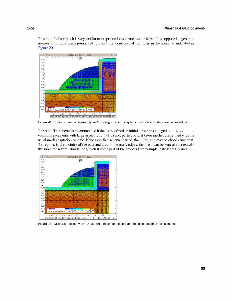
DIOS CHAPTER 4 GRID COMMAND
This modified approach is very similar to the protection scheme used in Mesh. It is supposed to generatemeshes with more mesh points and to avoid the formation of big holes in the mesh, as indicated inFigure 20.
Figure 20 Holes in mesh after using type=1D user grid, mesh adaptation, and default delaunization procedure
The modified scheme is recommended if the user defined an initial tensor product grid Grid(Type=1D,...)containing elements with large aspect ratio (> 1.5) and, particularly, if these meshes are refined with theusual mesh adaptation scheme. If the modified scheme is used, the initial grid may be chosen such that,for regions in the vicinity of the gate and around the mask edges, the mesh can be kept almost exactlythe same for several simulations, even if some part of the devices (for example, gate length) varies.
Figure 21 Mesh after using type=1D user grid, mesh adaptation, and modified delaunization scheme
95

DIOSCHAPTER 4 GRID COMMAND
96
DIOS CHAPTER 5 SUBSTRATE COMMAND
Dios
CHAPTER 5 Substrate command
5.1 OverviewThe Substrate command is used to initialize the layer system and to define the properties of the wafermaterial. The crystal orientation of the wafer surface, the background doping element, and its (constant)concentration are defined. Appendix D on page 335 lists the Substrate command parameters.
NOTE The default values of some parameters may depend on the crystal orientation. User-definedchanges of these default values are lost when executing the Substrate command. Therefore, itis not recommended to place any changes of default values before the Substrate command.
The position of the simulation domain in the layout plane can be specified as:
Substrate(Cut(0,0,1,0))
The first two values define the beginning, and the third and fourth values define the end point of a cutlinein the layout plane (that is, on the wafer), which is used for the 2D simulation. The two points arespecified in the layout coordinate system. The first coordinate is taken along the wafer flat (layout-X)and the second coordinate is perpendicular to the wafer flat (layout-Y).
The Dios x-axis always follows the cutline. The beginning of the cutline is taken as origin for the Diosx-axis. The direction of the cutline defines an ‘initial rotation angle’ for the ion implantation. In addition,the direction of the cutline and the position of its beginning are used to define the coordinatetransformation for files saved in the DF–ISE format. This is required for the correct placement of severalDios simulation results in 3D space if the data is used to construct 3D devices based on 1D and 2Dresults.
During a 1D or 2D simulation, the Dios y-axis is assumed to be perpendicular to the layout plane, thatis, along the outward normal to the wafer surface.
For the simulation of a 3D structure, instead of the two points of a cutline, four points that define arectangle in the layout plane should be specified. In this case, eight coordinate values are required inCut(...). The four points of the rectangle are supposed to be defined counterclockwise in the layoutplane. During the 1D and 2D parts of the 3D simulation, the first line segment of the rectangle is usedas Cut-line:
SUBStrate(Cut(0,0, 1,0, 1,1, 0,1))
Throughout the entire simulation, the line connecting the first two points defines the Dios x-axis. For the1D and 2D parts of a 3D simulation, the outward normal to the wafer surface defines the Dios y-axis.When switching to 3D the line, connecting the first point and last point defines the direction of the Dios
97
DIOSCHAPTER 5 SUBSTRATE COMMAND
y-axis and the Dios z-axis for the 3D simulation is assumed along the outward normal to the wafersurface (that is, the y-axis of the 2D simulation).
If a 3D bnd file or 3D grd file is loaded after performing some 2D process simulation, the coordinatetransformation defined in the file is ignored, and the first coordinate is assumed to be the same as theDios x-coordinate in the 2D simulation. When interpolating the 2D doping, there is no variation alongthe second coordinate in the loaded file.
The location and extension of the initial 1D/2D layer system in the x-direction and y-direction can bedefined directly by XLeft, XRight, YBottom, YTop. The initial (vertical) position of the substrate surfaceYSubs can be prescribed as well. Usually, none of these values should be specified, since the valuesspecified in the preceding Grid command are used by default:
For NewDiff=0: YSubs=YTopgrid and YTop=YSubs+2μm
For NewDiff=1: YTop=YTopgrid and YSubs=0
NOTE For NewDiff=1 (that is, by default), the initial user grid (usually Grid(y(y2=...))should bechosen large enough to at least contain the initial substrate together with the gas region, thatis, YTopgrid > YSubs.
Defining a too small initial grid may cause interpolation errors or sometimes strange behavior, forexample, of the Monte Carlo simulation. If necessary, Dios expands the grid automatically at the topduring the process steps. Some effort has been put into expanding the grid properly by adding pairs ofstripes of elements to the grid, avoiding jumping of the vertical position of mesh points, which used tobe a source of interpolation errors.
To avoid such problems, it is recommended to define the initial grid large enough to contain the entiresimulation domain, including the gas region during the entire process simulation. It is necessary toaccount for the thickness of epilayers and photoresist masks (for example, for contact hole etching andcontact patterning) already in the initial grid. Defining the initial user grid large enough (but withinreasonable extensions) does not cause any known problems.
In the Substrate command, the crystal orientation of the wafer surface can be specified asORIENtation=100, 110, or 111. By default, 100 material is assumed. The crystal orientation can bespecified only for the substrate. Other (for example, deposited) silicon layers are treated with the samecrystal orientation.
The background doping element (ELEMent=B) and the resistivity (RHO) [Ω cm] can be specified. IfRHO=undefined, the background doping CONCentration can be specified explicitly. If CONCentration is alsoundefined (or if no positive value is specified), no background doping is assumed for the simulation.
98
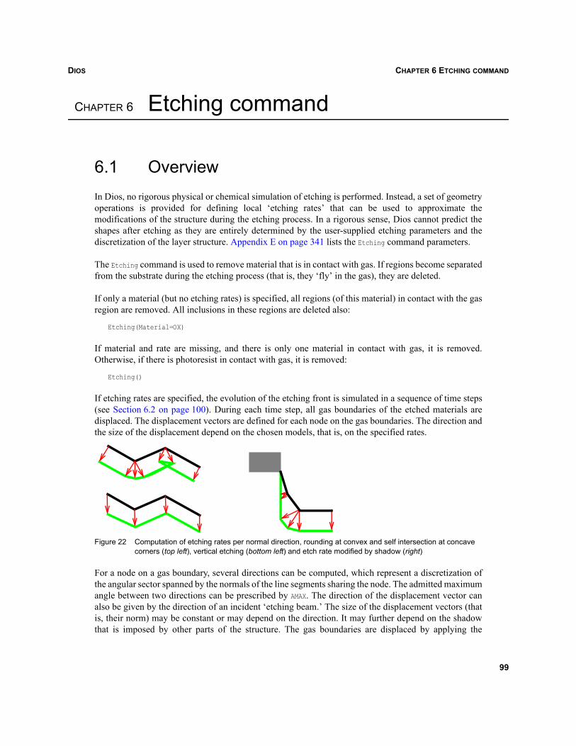
DIOS CHAPTER 6 ETCHING COMMAND
Dios
CHAPTER 6 Etching command
6.1 OverviewIn Dios, no rigorous physical or chemical simulation of etching is performed. Instead, a set of geometryoperations is provided for defining local ‘etching rates’ that can be used to approximate themodifications of the structure during the etching process. In a rigorous sense, Dios cannot predict theshapes after etching as they are entirely determined by the user-supplied etching parameters and thediscretization of the layer structure. Appendix E on page 341 lists the Etching command parameters.
The Etching command is used to remove material that is in contact with gas. If regions become separatedfrom the substrate during the etching process (that is, they ‘fly’ in the gas), they are deleted.
If only a material (but no etching rates) is specified, all regions (of this material) in contact with the gasregion are removed. All inclusions in these regions are deleted also:
Etching(Material=OX)
If material and rate are missing, and there is only one material in contact with gas, it is removed.Otherwise, if there is photoresist in contact with gas, it is removed:
Etching()
If etching rates are specified, the evolution of the etching front is simulated in a sequence of time steps(see Section 6.2 on page 100). During each time step, all gas boundaries of the etched materials aredisplaced. The displacement vectors are defined for each node on the gas boundaries. The direction andthe size of the displacement depend on the chosen models, that is, on the specified rates.
Figure 22 Computation of etching rates per normal direction, rounding at convex and self intersection at concave corners (top left), vertical etching (bottom left) and etch rate modified by shadow (right)
For a node on a gas boundary, several directions can be computed, which represent a discretization ofthe angular sector spanned by the normals of the line segments sharing the node. The admitted maximumangle between two directions can be prescribed by AMAX. The direction of the displacement vector canalso be given by the direction of an incident ‘etching beam.’ The size of the displacement vectors (thatis, their norm) may be constant or may depend on the direction. It may further depend on the shadowthat is imposed by other parts of the structure. The gas boundaries are displaced by applying the
99
DIOSCHAPTER 6 ETCHING COMMAND
displacement vectors to the nodes. After displacing the boundaries, the consistency of the layer systemmust be checked: self intersections of the moving boundary polygons and intersections with thenonmoving parts of the boundaries are removed, boundaries and areas are subdivided, and very smalllayers are deleted.
When the entire etching process is finished, the mesh is readapted to the new layer structure. The end ofthe etching process can be defined by prescribing the total etching Time, the amount of material that hasto be removed, or by defining an etch stop.
Remove defines the thickness that has to be etched away. It is translated into an etching time using the datafor the fastest etching rate.
An etch stop is defined by a list of materials or boundary sorts: STOP. If NSTop ≠ 0, the etching processstops if the number of areas or boundaries of the specified material or sort changes by NSTop. If NSTop isnot specified, the etching process is stopped at any change of this number. If INCstop=off is specified, theabsolute number of areas resp. boundaries, and not the number of changes, is checked. If the requiredabsolute number of areas or boundaries already exists, no etching is performed. The parameters STOP,NSTOP, and INCstop are defined as vectors (of size 4). This allows for the definition of more than one etchstop at the same time. For ANDstop=on, the etching process is stopped if all conditions are fulfilled at thesame time. For ANDstop=off (default), the etching stops if the first of the conditions is fulfilled.
NOTE The result of an etch stop depends on the simulated structure. For example, if no activetransistor region is contained in the simulation domain, instead of a thin implant oxide, theentire field oxide may be etched away. Although less convenient, the specification of etchingtime or removed thickness is preferred.
To stabilize the etching simulation, an overetching is simulated. An additional time OVERTime, removeOVERTHickness or a relative time (Over) in percent of the total etching time from the begin to the specifiedend of the etching process (stop, time, or remove) is used. By default, Over=10%.
6.2 Isotropic and nonisotropic etching ratesThe isotropic and nonisotropic components of the etching rates can be specified as:
Rate(Isotropic=... A0=... A1=... A2=... A3=...)
If the etching Time or Remove are specified but no etching rates, internally isotropic etching withIsotropic=100nm/min is assumed. The etching rates A0,...,A3 can be used to control the etching rate as afunction of the slope of the line segments. If only one positive value is specified for A1 (or A2 or A3), therewill remain ‘spacers’ at all layer edges with steep slopes. Sometimes, this is unwanted (for example, atsteep field oxide edges). In this situation, the rate constant A0 should be used rather than A1.
NOTE Pure A0 etching is not intended to be used for spacer etching.
100
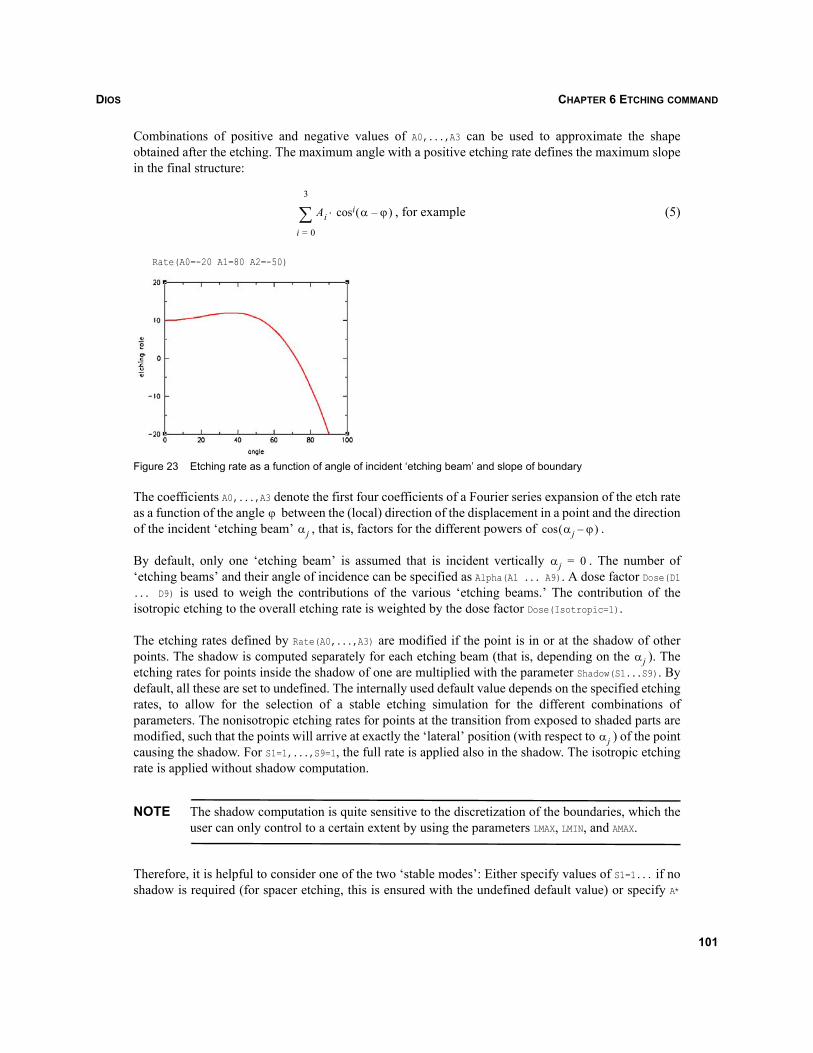
DIOS CHAPTER 6 ETCHING COMMAND
Combinations of positive and negative values of A0,...,A3 can be used to approximate the shapeobtained after the etching. The maximum angle with a positive etching rate defines the maximum slopein the final structure:
, for example (5)
Rate(A0=-20 A1=80 A2=-50)
Figure 23 Etching rate as a function of angle of incident ‘etching beam’ and slope of boundary
The coefficients A0,...,A3 denote the first four coefficients of a Fourier series expansion of the etch rateas a function of the angle between the (local) direction of the displacement in a point and the directionof the incident ‘etching beam’ , that is, factors for the different powers of .
By default, only one ‘etching beam’ is assumed that is incident vertically . The number of‘etching beams’ and their angle of incidence can be specified as Alpha(A1 ... A9). A dose factor Dose(D1... D9) is used to weigh the contributions of the various ‘etching beams.’ The contribution of theisotropic etching to the overall etching rate is weighted by the dose factor Dose(Isotropic=1).
The etching rates defined by Rate(A0,...,A3) are modified if the point is in or at the shadow of otherpoints. The shadow is computed separately for each etching beam (that is, depending on the ). Theetching rates for points inside the shadow of one are multiplied with the parameter Shadow(S1...S9). Bydefault, all these are set to undefined. The internally used default value depends on the specified etchingrates, to allow for the selection of a stable etching simulation for the different combinations ofparameters. The nonisotropic etching rates for points at the transition from exposed to shaded parts aremodified, such that the points will arrive at exactly the ‘lateral’ position (with respect to ) of the pointcausing the shadow. For S1=1,...,S9=1, the full rate is applied also in the shadow. The isotropic etchingrate is applied without shadow computation.
NOTE The shadow computation is quite sensitive to the discretization of the boundaries, which theuser can only control to a certain extent by using the parameters LMAX, LMIN, and AMAX.
Therefore, it is helpful to consider one of the two ‘stable modes’: Either specify values of S1=1... if noshadow is required (for spacer etching, this is ensured with the undefined default value) or specify A*
Ai α ϕ–( )cosi⋅
i 0=
3
∑
ϕαj αj ϕ–( )cos
αj 0=
αj
αj
101
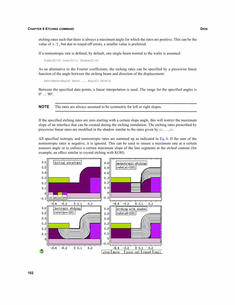
DIOSCHAPTER 6 ETCHING COMMAND
etching rates such that there is always a maximum angle for which the rates are positive. This can be thevalue of , but due to round-off errors, a smaller value is preferred.
If a nonisotropic rate is defined, by default, one single beam normal to the wafer is assumed:
Alpha(A1=0) Dose(D1=1) Shadow(S1=0)
As an alternative to the Fourier coefficients, the etching rates can be specified by a piecewise linearfunction of the angle between the etching beam and direction of the displacement:
Rate(ARate(Angle1 Rate1 ... Angle15 Rate15)
Between the specified data points, a linear interpolation is used. The range for the specified angles is0o … 90o.
NOTE The rates are always assumed to be symmetric for left or right slopes.
If the specified etching rates are zero starting with a certain slope angle, this will restrict the maximumslope of an interface that can be created during the etching simulation. The etching rates prescribed bypiecewise linear rates are modified in the shadow similar to the rates given by A0,...,A3.
All specified isotropic and nonisotropic rates are summed up as indicated in Eq. 6. If the sum of thenonisotropic rates is negative, it is ignored. This can be used to ensure a maximum rate at a certainnonzero angle or to enforce a certain maximum slope of the line segments at the etched contour (forexample, an effect similar to crystal etching with KOH).
π 2⁄
102
DIOS CHAPTER 6 ETCHING COMMAND
Several materials can be etched at the same time. In this case, the etching time or etch stops can bedefined. If a remove thickness is specified, it will be translated internally into an etching time by usingthe data for the fastest etching material. To define the etching rates, inside the data record Rate, first theMaterial must be specified, followed by the rate parameters for that material. Then, the next Material canbe defined, followed again by the rate parameters for that material:
Rate(Material=Si,Isotropic=100nm/min,Material=Ox,Isotropic=50nm/min)
If the parameters DAlpha=...degree, SIGma are specified, a series of nine etching beams is assumed. AGaussian distribution with the standard deviation DAlpha is assumed for the incidence angles around thedirection Alpha(A1=). A second Gaussian distribution with the standard deviation SIGma is assumed for thedose of these etching beams. The Shadow values S1...S9 are all set to 0 by default.
The isotropic or nonisotropic etching rate in a point of the Dios layer system in the direction isgiven by:
(6)
Here, m denotes the material of the point, j the number of the ion beam, and if the point isexposed by the beam j; otherwise, (the value in the shadow). The parameters and define the dose and the direction of the beam. denotes the (material-dependent) nonisotropic ratecoefficients, denotes the isotropic dose, and denotes the isotropic rate. The function denotes the etching rate defined per material and the ion beam direction, by linear interpolation on thevalues of ARate.
6.3 Vertical etchingPurely directional etching in the direction of the incident etching beam is assumed if the etching rate isspecified as Rate(Anisotropic).
NOTE Anisotropic is no longer a synonym of A1. Anisotropic can be specified to perform a strictlyvertical etching (since Alpha(A1=0) by default).
The constructed shapes are similar to the ones created by A0 etching. This is most useful if exactly onematerial is etched with the help of a mask and if perfectly vertical walls are expected as a result.Anisotropic etching rates cannot be combined with the other types of rate specification. In this case, Diosgenerates a warning and replaces Anisotropic with A1. The Anisotropic etching can be applied if theetching front contains vertical boundaries, but it cannot be used if the structure contains already‘overhanging’ parts at the gas boundary. These parts may actually grow instead of being etched or mayremain unchanged. The admitted ‘overhang’ is determined by the parameter ShadowSmall. If the‘overhang’ is smaller than admitted, the ‘overhang’ is removed and vertical etching is applied. If the‘overhang’ is larger, an A1 etching is assumed instead.
x y,( ) ϕ
r Diso I m( )⋅ δj x y,( ) Dj⋅
j 1=
k
∑+ AR αj ϕ m,–( ) Ai m( ) αj ϕ–( )cosi⋅
i 0=
3
∑+⎝ ⎠⎜ ⎟⎜ ⎟⎛ ⎞
⋅=
δj x y,( ) 1=δj x y,( ) Sj= Dj αj
Ai m( )Diso I m( ) AR
103
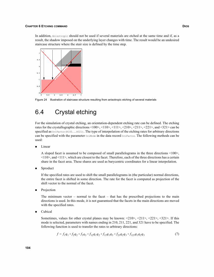
DIOSCHAPTER 6 ETCHING COMMAND
In addition, Anisotropic should not be used if several materials are etched at the same time and if, as aresult, the shadow imposed on the underlying layer changes with time. The result would be an undesiredstaircase structure where the stair size is defined by the time step.
Figure 24 Illustration of staircase structure resulting from anisotropic etching of several materials
6.4 Crystal etchingFor the simulation of crystal etching, an orientation-dependent etching rate can be defined. The etchingrates for the crystallographic directions <100>, <110>, <111>, <210>, <211>, <221>, and <321> can bespecified as OriFactor(R100...R321). The type of interpolation of the etching rates for arbitrary directionscan be specified with the parameter OriMode in the data record OriFactor. The following methods can beused:
Linear
A sloped facet is assumed to be composed of small parallelograms in the three directions <100>,<110>, and <111>, which are closest to the facet. Therefore, each of the three directions has a certainshare in the facet area. These shares are used as barycentric coordinates for a linear interpolation.
Sproduct
If the specified rates are used to shift the small parallelograms in (the particular) normal directions,the entire facet is shifted in some direction. The rate for the facet is computed as projection of theshift vector to the normal of the facet.
Projection
The minimum vector – normal to the facet – that has the prescribed projections to the maindirections is used. In this mode, it is not guaranteed that the facets in the main directions are movedwith the specified rates.
Cubical
Sometimes, values for other crystal planes may be known: <210>, <211>, <221>, <321>. If thismode is selected, parameters with names ending in 210, 211, 221, and 321 have to be specified. Thefollowing function is used to transfer the rates to arbitrary directions:
(7)f f1q1 f2q2 f3q3 f12q1q2 f13q1q3 f23q2q3 f123q1q2q3+ + + + + +=
104
DIOS CHAPTER 6 ETCHING COMMAND
where denotes the area shares as in the linear mode.
HalfAngle
Similar to CUbical, except that the intermediate values are assumed to describe not the rates normalto the particular planes, but the rates in the three directions, bisecting the angles and in the spatialdirection that has the same deviation from all three main directions.
Isotropic
The same rate is used in all directions. This is the default.
6.5 Controlling etching simulationsThe changes in the layer system in the simulation of etching (as well as deposition, epitaxy, oxidation,and glass reflow) are calculated using the same string algorithm. The old and new boundaries arerepresented by polygons (open or closed). The new boundary is calculated from the old one by applyingthe computed displacements of the boundary motion in an explicit time step followed by a de-loopingof first the new boundary and then all boundaries of the layers that are modified during the etching step.The result of the string algorithm is controlled to a large extent by the local time step size, thediscretization along the moving interfaces, and the discretization of the angular sector a point can movein.
To control the advancement of the etching front, the time step DT, the number of etching steps Steps, orthe displacement per time step DThickness can be prescribed. DThickness=10nm is the internal default. Forstability reasons, the first time step is always chosen smaller by a factor First. In general, the maximumdisplacement of the moving front per time step will restrict the amount of overlap or (self-)intersectionsof the moving front with itself or with other boundaries of the same layer. The smaller the displacementper time step, the smaller the error can be expected. For deposition processes, a default of 10 time stepsis used. For etching, epitaxy, and oxidation processes, a maximum displacement of 10 nm per time stepis used by default. For the high temperature steps, the time step is limited also by the convergence of theNewton iteration.
In order to avoid topology errors caused by round-off errors and to ensure always a well-definedrelationship between old and new boundaries for all points, a minimum displacement per time step isdefined (even if parts of the boundary are supposed to be immobile). The parameter DMIN defines thisminimum. It should always be set to a very small but strictly positive value.
The parameters LMIN and LMAX control the spatial resolution along the moving boundaries. They definethe range of distances between ‘neighboring’ points along the boundaries. If the distance is greater thanLMAX, additional points are inserted before the boundary is moved. If the distance is below LMIN, pointsare removed before and after the boundary is moved. In general, smaller values lead to better resolutionwith increased time and storage effort.
NOTE The default value of LMAX is chosen in accordance to the finest resolution of the mesh: fromthe minimum edge length in the user grid, and the global values of the MaxTrl andRefineBoundary (if <0).
qi
105
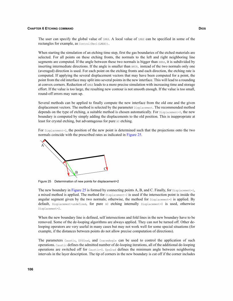
DIOSCHAPTER 6 ETCHING COMMAND
The user can specify the global value of LMAX. A local value of LMAX can be specified in some of therectangles for example, as Control(Rec1(LMAX)).
When starting the simulation of an etching time step, first the gas boundaries of the etched materials areselected. For all points on these etching fronts, the normals to the left and right neighboring linesegments are computed. If the angle between these two normals is bigger than AMAX, it is subdivided byinserting intermediate directions. If the angle is smaller than AMIN, instead of the two normals only one(averaged) direction is used. For each point on the etching fronts and each direction, the etching rate iscomputed. If applying the several displacement vectors that may have been computed for a point, thepoint from the old interface may split into several points in the new interface. This will lead to a roundingat convex corners. Reduction of AMAX leads to a more precise simulation with increasing time and storageeffort. If the value is too large, the resulting new contour is not smooth enough. If the value is too small,round-off errors may sum up.
Several methods can be applied to finally compute the new interface from the old one and the givendisplacement vectors. The method is selected by the parameter Displacement. The recommended methoddepends on the type of etching, a suitable method is chosen automatically. For Displacement=0, the newboundary is computed by simply adding the displacements to the old position. This is inappropriate atleast for crystal etching, but advantageous for pure A0 etching.
For Displacement=2, the position of the new point is determined such that the projections onto the twonormals coincide with the prescribed rates as indicated in Figure 25.
Figure 25 Determination of new points for displacement=2
The new boundary in Figure 25 is formed by connecting points A, B, and C. Finally, for Displacement=1,a mixed method is applied. The method for Displacement=2 is used if the intersection point is inside theangular segment given by the two normals; otherwise, the method for Displacement=0 is applied. Bydefault, Displacement=undefined, for pure A0 etching internally Displacement=0 is used, otherwiseDisplacement=2.
When the new boundary line is defined, self intersections and fold lines in the new boundary have to beremoved. Some of the de-looping algorithms are always applied. They can not be turned off. Other de-looping operators are very useful in many cases but may not work well for some special situations (forexample, if the distances between points do not allow precise computation of directions).
The parameters Caustic, EPSGrad, and CoarseAngle can be used to control the application of suchoperations. Caustic defines the admitted number of de-looping iterations, all of the additional de-loopingoperations are switched off for Caustic=0. EpsGrad defines the minimum angle between neighboringintervals in the layer description. The tip of corners in the new boundary is cut off if the corner includes
A
BC
106
DIOS CHAPTER 6 ETCHING COMMAND
an angle smaller than EPSGrad. CoarseAngle is used to check if a point can be removed from the admittedangle between intervals when deciding to remove a point. Points that are very close to each other arealways removed. If the boundary has been changed, a new de-looping iteration is started.
After de-looping, the new line is added into the existing layer system. Intersections with otherboundaries are detected and the necessary corrections are performed (for example, subdivision orremoval of areas). Since this may include sometimes very small areas of very short boundary lines, inDios, no precise control of the area and boundary names can be given to the user and the names aregenerated automatically. This may sometimes even lead to overflow of the total number of admittedareas and boundaries. One can use the Dios graphics to analyze the situation and maybe either modifythe etching command or select a smaller simulation area. Due to the explicit time discretization of thegeometry operations, spatial resolution and time step should be chosen carefully. Physicallyunmotivated corners in the geometry indicate a time step that is probably too large for the given spatialresolution.
The global parameters AMIN, AMAX, DMIN, LMIN, LMAX, and CoarseAngle are defined in each of the commands.Changing the default values must be done individually for the Deposit, ETCHing, and Diffusion commands.The parameters Caustic and EPSGrad can be defined globally for all process steps in the Control parameterrecord.
6.6 Polygon etchingDios gives users the capability to modify geometry (regions and materials) using the ‘trapezoidaletching’ feature. To do this, instead of the Etching command, the LControl(Cut...) command must beused (see Appendix U on page 597).
This allows, in particular, to cut specified material by a polygon in two parts, with the remaining oldmaterial in one part, and creating a new material in the other part.
LControl:(Cut(CutMaterial=<material_to_cut> CreateMaterial=<new_material> x1= y1= ... x20= y20=))
In the above command, x1, y1, ... define the coordinates of the cut polygon (up to 20 points areallowed). The polygon can be open, that is, assumed to be a directed multiline. The left and right sidesof the line are defined when walking from the first to the last point of the polygon. Only<material_to_cut> is affected: the region to the left of the polygon is replaced with <new_material> and theregion to the right is unchanged.
6.7 ExamplesRemove all resist regions at the surface:
Etching(Resist)
Nonisotropic etching of oxide, until silicon or polysilicon are in contact with gas:
Etching(Material=OX,STOP=(SIGAS,POGAS), Rate(Anisotropic=100))
107
DIOSCHAPTER 6 ETCHING COMMAND
Etching of a deep trench:
Etching(Material=si,Shadow(0.2),Rate(A1=600,A3=100),Remove=4um, Over=0.)
Etching(Material=si,Remove=4um,Over=0,Rate(Isotropic=10nm/min,A1=740nm/min,A3=150nm/min))
Nonisotropic etching of oxide, until silicon (at two places) and polysilicon are in contact with gas:
ETCHing(MATerial=OX,STOP=(SIGAS,POGAS),NSTop(2),ANDstop,Rate(Anisotropic=100))
Isotropic etching of 100 nm nitride, selectivity of all the other materials to nitride is 1:100:
ETCHing(MATerial=Ni,REmove=100nm,SELectivity=0.01)
Purely nonisotropic etching of 100 nm oxide from the right top direction in an angle of 45 ± 1 degreesimulated with 20 time steps:
ETCHing(MATerial=Ox,REmove=100nm,Rate(A1=1),Alpha=45,Sigma=1,STeps=20)
Nitride etching with sputtering effect:
ETCHing(MATerial=Ni,Time=100min,Rate(A1=1.5nm/min,A0=-0.5nm/min))
Nonisotropic silicon and isotropic oxide etching:
ETCHing(Time=100min,Rate(MATerial=Si,A1=1nm/min,MATerial=Ox,Isotropic=1nm/min))
Isotropic etching of silicon. For polysilicon, the same etching properties are assumed. Selectivityoxide:silicon=1:10:
ETCHing(Material=Si,Time=100min,Rate(Isotropic=1,Material=Po,EtchMaterial=Si,Material=Ox,Selectivity=0.1))
Etching of a deep trench with prescribed maximum slope:
ETCHing(Material=SI,Remove=350nm,Over=0,Rate(ARate(0.,0.,30.,0.,30.1,100,85,100,85.1,0)))
108
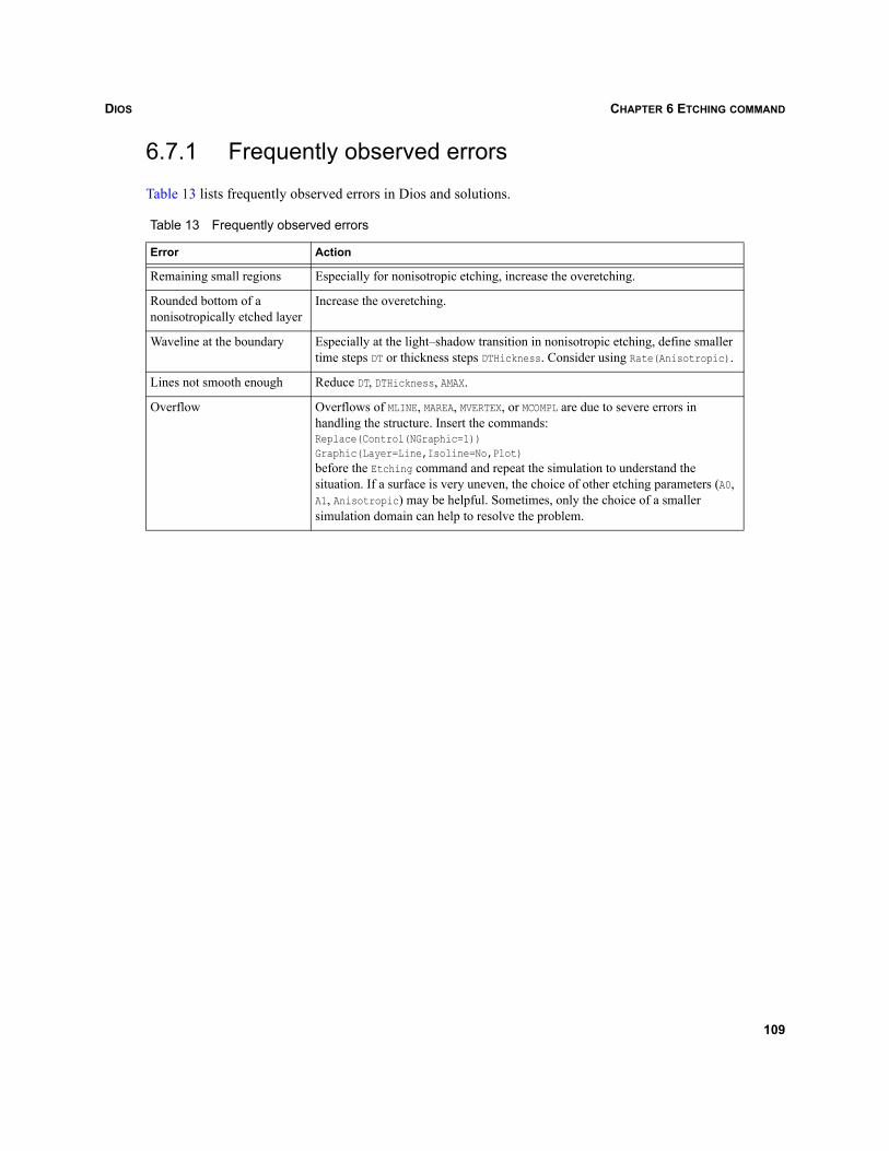
DIOS CHAPTER 6 ETCHING COMMAND
6.7.1 Frequently observed errors
Table 13 lists frequently observed errors in Dios and solutions.
Table 13 Frequently observed errors
Error Action
Remaining small regions Especially for nonisotropic etching, increase the overetching.
Rounded bottom of a nonisotropically etched layer
Increase the overetching.
Waveline at the boundary Especially at the light–shadow transition in nonisotropic etching, define smaller time steps DT or thickness steps DTHickness. Consider using Rate(Anisotropic).
Lines not smooth enough Reduce DT, DTHickness, AMAX.
Overflow Overflows of MLINE, MAREA, MVERTEX, or MCOMPL are due to severe errors in handling the structure. Insert the commands:Replace(Control(NGraphic=1))Graphic(Layer=Line,Isoline=No,Plot)before the Etching command and repeat the simulation to understand the situation. If a surface is very uneven, the choice of other etching parameters (A0, A1, Anisotropic) may be helpful. Sometimes, only the choice of a smaller simulation domain can help to resolve the problem.
109

DIOSCHAPTER 6 ETCHING COMMAND
110
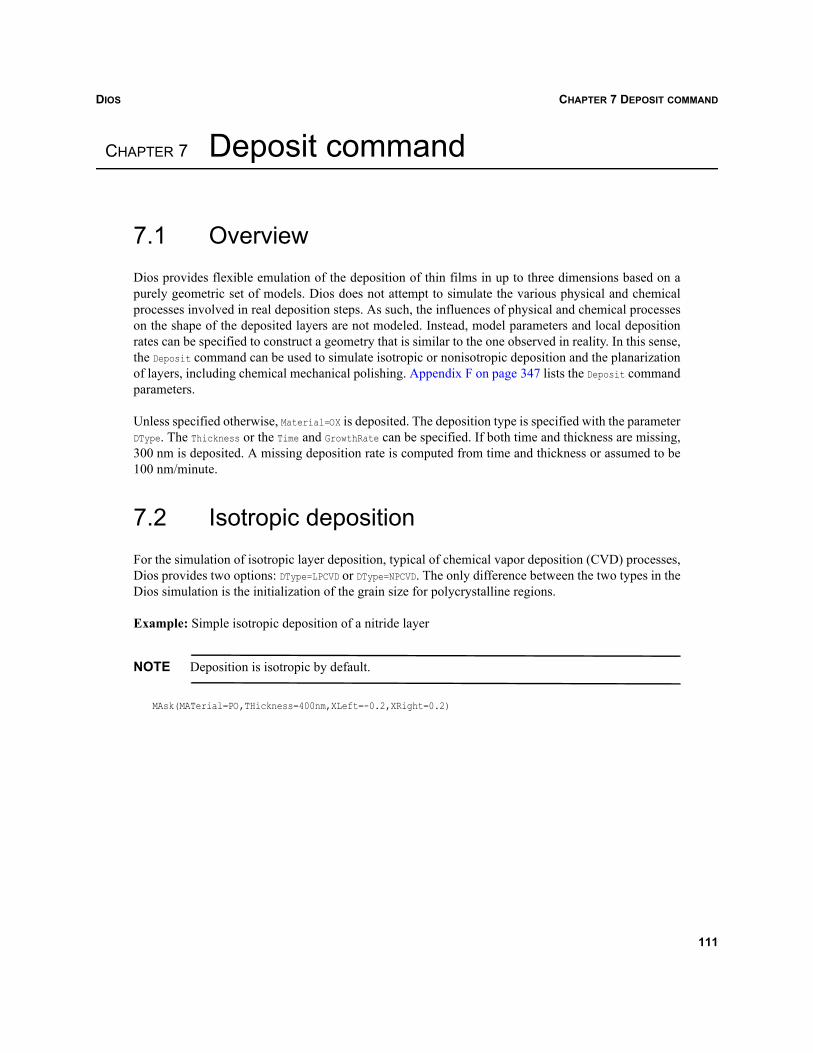
DIOS CHAPTER 7 DEPOSIT COMMAND
Dios
CHAPTER 7 Deposit command
7.1 OverviewDios provides flexible emulation of the deposition of thin films in up to three dimensions based on apurely geometric set of models. Dios does not attempt to simulate the various physical and chemicalprocesses involved in real deposition steps. As such, the influences of physical and chemical processeson the shape of the deposited layers are not modeled. Instead, model parameters and local depositionrates can be specified to construct a geometry that is similar to the one observed in reality. In this sense,the Deposit command can be used to simulate isotropic or nonisotropic deposition and the planarizationof layers, including chemical mechanical polishing. Appendix F on page 347 lists the Deposit commandparameters.
Unless specified otherwise, Material=OX is deposited. The deposition type is specified with the parameterDType. The Thickness or the Time and GrowthRate can be specified. If both time and thickness are missing,300 nm is deposited. A missing deposition rate is computed from time and thickness or assumed to be100 nm/minute.
7.2 Isotropic depositionFor the simulation of isotropic layer deposition, typical of chemical vapor deposition (CVD) processes,Dios provides two options: DType=LPCVD or DType=NPCVD. The only difference between the two types in theDios simulation is the initialization of the grain size for polycrystalline regions.
Example: Simple isotropic deposition of a nitride layer
NOTE Deposition is isotropic by default.
MAsk(MATerial=PO,THickness=400nm,XLeft=-0.2,XRight=0.2)
111
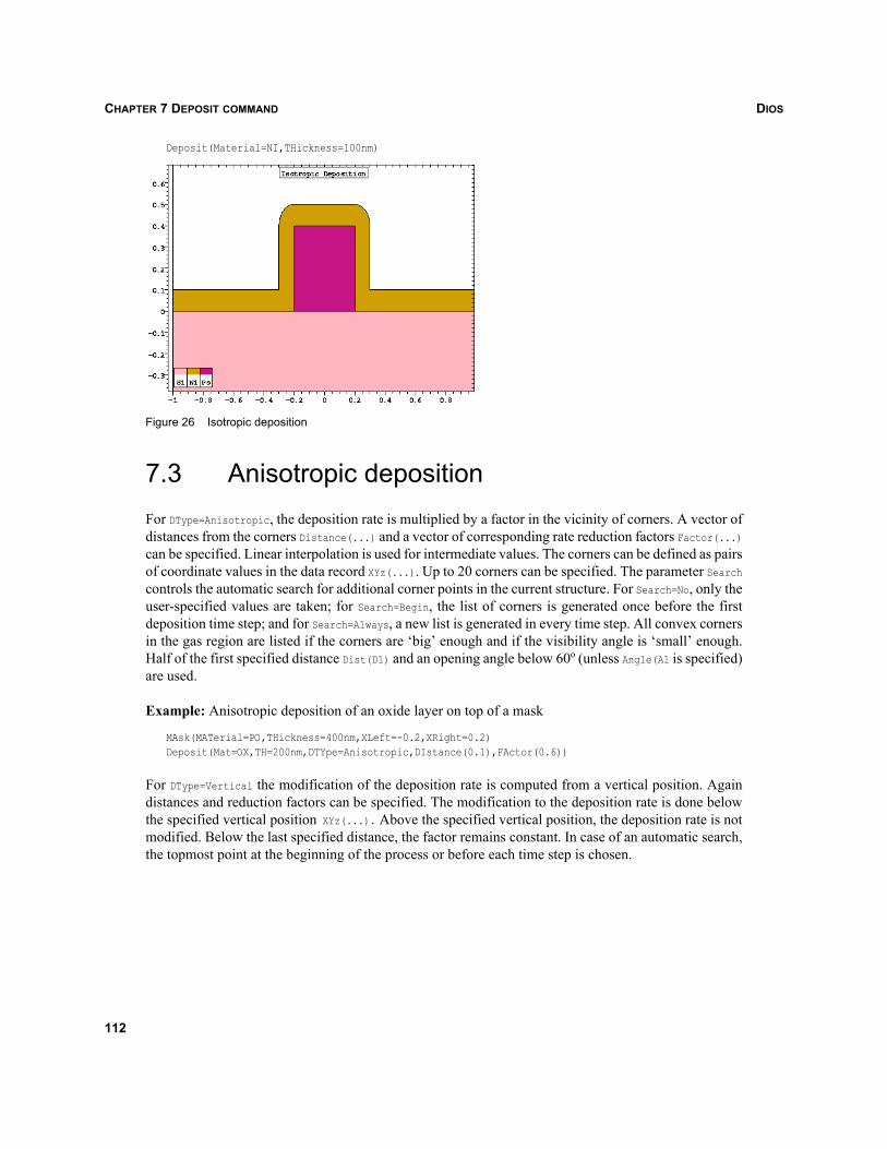
DIOSCHAPTER 7 DEPOSIT COMMAND
Deposit(Material=NI,THickness=100nm)
Figure 26 Isotropic deposition
7.3 Anisotropic depositionFor DType=Anisotropic, the deposition rate is multiplied by a factor in the vicinity of corners. A vector ofdistances from the corners Distance(...) and a vector of corresponding rate reduction factors Factor(...)can be specified. Linear interpolation is used for intermediate values. The corners can be defined as pairsof coordinate values in the data record XYz(...). Up to 20 corners can be specified. The parameter Searchcontrols the automatic search for additional corner points in the current structure. For Search=No, only theuser-specified values are taken; for Search=Begin, the list of corners is generated once before the firstdeposition time step; and for Search=Always, a new list is generated in every time step. All convex cornersin the gas region are listed if the corners are ‘big’ enough and if the visibility angle is ‘small’ enough.Half of the first specified distance Dist(D1) and an opening angle below 60o (unless Angle(A1 is specified)are used.
Example: Anisotropic deposition of an oxide layer on top of a mask
MAsk(MATerial=PO,THickness=400nm,XLeft=-0.2,XRight=0.2)Deposit(Mat=OX,TH=200nm,DTYpe=Anisotropic,DIstance(0.1),FActor(0.6))
For DType=Vertical the modification of the deposition rate is computed from a vertical position. Againdistances and reduction factors can be specified. The modification to the deposition rate is done belowthe specified vertical position XYz(...). Above the specified vertical position, the deposition rate is notmodified. Below the last specified distance, the factor remains constant. In case of an automatic search,the topmost point at the beginning of the process or before each time step is chosen.
112
DIOS CHAPTER 7 DEPOSIT COMMAND
Figure 27 Anisotropic deposition
Example: Nonisotropic deposition of an oxide layer on top of a mask
MAsk(Material=Po,THickness=400nm,XLeft=-0.5,XRight=0.5)Deposit(Mat=OX,TH=200nm,DTYPe=Vertical,DIstance(0.1),FACtor(1.05))
For Dtype=Angle, the deposition rate is modified depending on the visibility angle at each point. A list ofangles Angle and corresponding factors Factor(...) are specified. For each point, the visibility angle ofthe gas region is computed. This angle is used to interpolate the reduction factor for the deposition rate.
In addition, the deposition can be combined with a (partial) etchback of the deposited layers. This canbe used to mimic the effect of sputter deposition. The ‘etching’ rates can be specified as in the Etchingcommand (Rate, OriFactor, Alpha, Shadow, Dose; see Chapter 6 on page 99). During the simulation of onetime step, first the deposition step is simulated, followed by the etching time step. This includes the fullde-looping procedures as in the etching simulation. A new layer will grow only if, at least locally, thedeposition rate exceeds the etching rates (multiplied with the Dose values).
For DType=Fill, the structure is filled (planarized) up to a certain position YFill, which must be above theentire layer stack of the current layer system. The user can prescribe the value. If the value YFill ismissing or has been specified too small such that not the entire layer structure would be covered by thenew layer, the value is chosen internally at the topmost position in the existing layer system plus 1 nm.(Partial filling up to a certain height must be simulated with a combination of filling followed byetchback.) DType=Fill, in combination with etching steps, can be used to mimic the result of a chemical-mechanical polishing (CMP) step.
Example: Planarization
Deposit(Material=OX,DType=Fill,YFill=2.um)
113
DIOSCHAPTER 7 DEPOSIT COMMAND
7.4 Angle-dependent anisotropic depositionA more flexible capability for anisotropic deposition is available. The definition is similar to theanisotropic etching including the shadow computation, see Section 6.2 on page 100:
Deposition(GrowthRate(A0= A1= A2= A3= Isotropic=ARate(Angle1= Rate1=... Angle15= Rate15=)))
During the deposition, a minimum deposition rate is always applied. (The version of the string algorithmincludes only a limited topology checker.) At the end of the nonisotropic deposition, the summed upminimum displacements are etched away. On smooth surface parts, this should leave bare surface inplaces, where it is desired. It is not recommended to use both nonisotropic deposition and etchback:
ETCHing:(DrawRates:=on/off)
The angular distribution of the etching rates specified in the Etching command can be displayed. If youspecify also File="aaa.plx", a .plx file with this angular distribution is generated.
7.5 Selective depositionSelective deposition of silicon can be simulated using the Selection switch with the options:
Selection=AllSiPo Deposit crystalline Si on crystalline Si; Polysilicon on all other materials.
Selection=OnlySiPo Deposit crystalline Si on Si, Po on Po, and no deposition on all other materials.
Example: Selective epitaxial growth of an elevated source/drain structure
Taken from the Manual Examples Library Example_Library/Tools/Dios/2D/Selective_Epitaxy/
Elevated_Source_Drain:
Deposit(Material=Si,Selection=OnlySiPo,THick=50nm, ELe=P, CONC=1E14)
NOTE Selective deposition is ignored (that is, Selection reverts to the default AllDepoMat) if the usertries to use selective deposition for materials other than Si and Po.
7.6 Generating a mesh after depositionAt the end of the deposition step, a new grid is constructed, which contains the new material boundaries.Usually, a complete mesh adaptation is performed in order to properly resolve the new materialboundaries. The mesh points of the new grid that belong to materials/regions that existed before thedeposition receive data values interpolated from the old grid. The values for the mesh points in the newlygrown layers have to be defined by the user. A constant value can be prescribed for each of the Diosvariables. If not specified, the default values known for each of the species are used. In Section Q.3 onpage 584, Concentration(AsTotal) defines constant values for each variable in the newly grown layer. If
114
DIOS CHAPTER 7 DEPOSIT COMMAND
only one single total dopant concentration is defined, Dios still accepts the outdated input: Element=As,Concentration=1e12.
Constant initial values for non-concentration type datasets (such as stress components and density) haveto be defined also as Concentration(Species). Data related to the initial grain size of polycrystalline layersis treated differently. The user can prescribe the initial grain sizes explicitly as: GrainSize(GrainShare=...GrainSize=... GrainSizeNormal=...). Alternatively, the initial grain size is computed from deposited layerthickness, DType and deposition Temperature.
If before the deposition there was already a region of the deposited material in contact with gas inexistence in the grid, Dios takes care to correctly separate the doping values between the already existinglayer and newly deposited regions of the same material. This is performed by temporarily assigning thenewly deposited regions a different material property. This may seem confusing if a graphic is displayedduring the deposition simulation, for example, NGraphic>0, but it is corrected at the end of the depositionstep.
If Deposit(Adaptation=on) is defined (that is, by default), the interfaces between old and new regions arerefined. The different material properties ensure the insertion of the interfaces between old and newregions into the grid. If the new grid has been generated and all values have been interpolated from theold grid, the material of the new regions is set to the correct value, and the doping and grain sizes in thenewly grown layer are overwritten by the user-defined or default constant values. The interfacesbetween old and new areas of the same material are removed from the layer structure.
In a second adaptation step, only the refinement according to steep doping gradients can ensure therequired resolution of the interface between old and new parts. For Deposit(Adaptation=off), noadaptation is foreseen, only the interfaces are inserted. In the first step, the old and new materials aredifferent, then the material of the new region is set to the one deposited, the doping values are initializedand, in the second step, the interface between old and new regions is no longer inserted.
If for both old and new regions different names had been specified by the user, the interfaces betweenregions of the same material are always kept in the layer system. These user-defined names must notcontain a number, followed by the string .area for example, 4.area. With Replace(Control(Imagin=on)),these interfaces are inserted into the grid. This is not recommended.
For NewDiff=0, the user-defined constant doping values are transferred to the grid points only if silicon isdeposited and the substrate region is enlarged (that is, if the deposition is simulated as a replacement foran epitaxy step). For NewDiff=0, the constant doping value specified in the deposition of materials otherthan crystalline silicon is stored separately (only one species and one value per material, not per area).These values are used later during the concentration-dependent oxidation (for example, of polysilicon).
The construction of the new boundary is performed in a very similar way to the simulation of the etching(see Section 6.5 on page 105). The same internal program modules are used to first construct thedisplacement vectors, to compute the new contours, to de-loop them, to resolve all global intersections(detect cavity formation), and to control the discretization: along the moving boundaries of the angularsectors, the points move in and of the size of the displacements.
115

DIOSCHAPTER 7 DEPOSIT COMMAND
116
DIOS CHAPTER 8 MASK COMMAND
Dios
CHAPTER 8 Mask command
8.1 OverviewMask regions composed of photoresist (or other materials) can be defined with the Mask command. Thelateral begin and end position of a mask region can be defined by the user or mask positions can also beread from an external input file. If the user wants to extract the mask positions directly from the layout,the Synopsys tool Ligament should be used to specify the process flow, the mask file, and the positionof the cutline of the Dios simulation. Appendix G on page 353 lists the Mask command parameters.
The Mask command allows specification of the Material, Thickness, and the lateral position of the maskcorners. The mask contours are constructed by default with a planar top surface, the minimum thicknessis determined by the parameter Thickness. The topmost point of all materials except photoresist isdetermined and the prescribed thickness of the mask is added to the vertical coordinate.
The lateral position of the mask edges, XLeft, XRight, or X=(...), is critical for obtaining good results. Theedges should not be located too close to the simulation boundaries. Typically, one edge is located welloutside the simulation domain and one is located inside (but not too close to the edge). Alternatively, thesimulation domain must be bounded by real symmetry lines to reduce the impact of the assumedsymmetry (or reflective) boundary conditions at the left and right side of the device. At the end of eachDios simulation, a simple check is performed. If a p-n junction at the left or right side of the device isdeeper than the minimum distance from any mask edge to this side, a 1D cross section is saved to a fileand a warning is given. The profile at the left or right side may change if a larger domain is specifiedand may also differ from 1D simulation results.
The slope Alpha of the mask edge can be specified, or a sequence of distances from the mask edges DxLeftand of corresponding mask thicknesses DThLeft can be specified to describe the mask shape at the leftand right mask edges. If nonsymmetric masks are required, separate values DxRight and DThRight can bespecified. In contrast to the Deposit command, the thickness of a mask is assumed to define the verticaloffset (not the normal offset) of the mask. The Mask command is used for relatively planar surfaces orinfinitely high masks. The user can also use the Deposit command (for example, with DType=Fill), Maskcommand, and Etch command to construct the masks. The rules for initialization of datasets and namingof layers are the same as for the Deposit command (see Section 7.6 on page 114).
8.2 Examples of mask statementsA photoresist mask covering the entire simulation domain:
Mask(Material=Resist,Thickness=1.5um)
Sloped nitride mask at the right side of the domain:
Mask(Material=Ni,Thickness=1,XLeft=5.0, Alpha=45degree)
117
DIOSCHAPTER 8 MASK COMMAND
Mask with profile:
Mask(Material=PO,XLeft=1.,XRight=5. DX=(0.1,0.2,0.3),DTH=(0.3,0.37,0.4))
8.3 Using an external mask file in a 2D simulationThe position of mask edges can alternatively be read from a file. The name of the mask file can bespecified as:
dios -mask="file" command
on the command line, when starting Dios or in the mask command. A particular mask from the mask fileis selected with the parameter Mask="name". The name of the mask file can also be specified in the (first)mask command in the Dios input file as File="name". The name of the currently used mask file and themask file itself are stored in the Dios dmp files. After loading the dmp file, Dios tries to continue to readmasks from this file. The mask file name must have the extension .pl1.
8.3.1 Structure of mask file
The first line, containing exactly one real number, is interpreted as the scaling factor. The second linedefines the minimum and maximum positions of masks. The third line contains the number of masks.
Then, the masks are defined. Each mask block has the following structure: The first line contains themask name and the number of mask segments. A mask name must not be an integer number, or start witha slash or percent character. Subsequent lines define the position of the mask edges for each segment.The positions are given as integer numbers. These values, divided by the scaling factor, define the lateralposition of the masked parts in μm. These numbers are interpreted as x-values in the 2D Dios coordinatesystem.
The mask file can contain comments. They must start with a slash (/) or percent (%) character.
Examples
A mask is defined using the external mask file:
Mask(Material=Resist, Thickness=1.0um, File=mask.pl1, Mask=Field)
The following is an example of an external mask file:
1000.00 60002%masksField 20 20004000 6000Poly 10 500
118
DIOS CHAPTER 9 IMPLANTATION COMMAND
Dios
CHAPTER 9 Implantation command
9.1 OverviewIn Dios, the simulation of implant steps is achieved using either analytic distribution functions or MonteCarlo simulation to compute the distribution of implanted ions and of implantation damage.
Algorithms for the analytic implantation into 1D and 2D structures are an integral part of the simulatorDios. The algorithm for analytic implantation into 3D structures was developed and implemented atFHG Erlangen [58]. The Monte Carlo simulation for 1D and 2D structures is performed with theprogram Crystal-TRIM [59] and is linked to the Dios binary, whereas the Monte Carlo simulation for3D structures is performed with the external tool MCimpl, which uses an algorithm developed at TUVienna [60]. Both external algorithms for 3D analytic and Monte Carlo simulation are controlled byDios, which generates input files of the required special formats, calls the appropriate conversion tools,and provides the appropriate command line options to the 3D meshing tool Mesh.
An implant step in Dios is specified by a set of keywords. The most essential keywords are ELEMent, DOse,ENergy, Tilt, and ROTation, for example:
Implantation(ELEMent=As,Dose=5e14,Energy=50,Tilt=0,ROTation=-90)
The implantation Dose is defined in Dios as particles per cm2 of the wafer surface. It does not depend onthe orientation of the wafer to the ion beam during the implantation. The default unit for energy is keV.The meaning and implications of tilt and rotation are discussed in Section 9.2.
For Function=Load2DMC, a precomputed 2D Monte Carlo simulation result can be loaded. The file namecan be specified only globally as Implantation(File=name.exp,...). Only the Dios file formats exp or prfcan be used. If the specified file cannot be read or no file name is supplied, Dios switches to Monte Carlosimulation and saves the as-implanted data. In this sense, Function=Load2DMC saves simulation time,whenever this is appropriate, and a simulation result can be repeatedly used (in a rerun or for a similarstructure).
Appendix H on page 355 lists the Implantation command parameters.
9.2 Wafer coordinate systemWhen defining an ion implant step, in addition to ELEMent, Energy, and Dose, it is important to consider theRotation and Tilt parameters. The specified values of ROTation and Tilt define the orientation of thewafer with respect to the (3D) incident ion beam. To better appreciate the relevance of Rotation and Tilt,it is first useful to understand the wafer coordinate system with respect to the fixed 3D frame of the ionbeam.
119
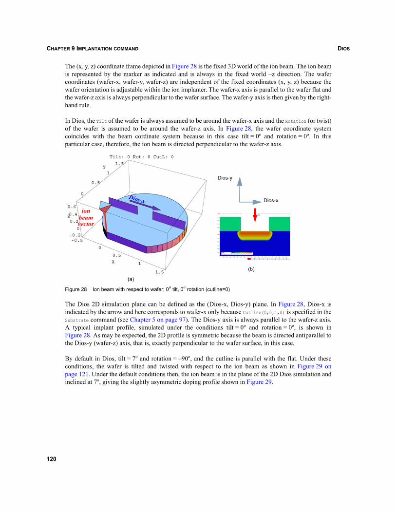
DIOSCHAPTER 9 IMPLANTATION COMMAND
The (x, y, z) coordinate frame depicted in Figure 28 is the fixed 3D world of the ion beam. The ion beamis represented by the marker as indicated and is always in the fixed world –z direction. The wafercoordinates (wafer-x, wafer-y, wafer-z) are independent of the fixed coordinates (x, y, z) because thewafer orientation is adjustable within the ion implanter. The wafer-x axis is parallel to the wafer flat andthe wafer-z axis is always perpendicular to the wafer surface. The wafer-y axis is then given by the right-hand rule.
In Dios, the Tilt of the wafer is always assumed to be around the wafer-x axis and the Rotation (or twist)of the wafer is assumed to be around the wafer-z axis. In Figure 28, the wafer coordinate systemcoincides with the beam cordinate system because in this case tilt = 0o and rotation = 0o. In thisparticular case, therefore, the ion beam is directed perpendicular to the wafer-z axis.
Figure 28 Ion beam with respect to wafer; 0o tilt, 0o rotation (cutline=0)
The Dios 2D simulation plane can be defined as the (Dios-x, Dios-y) plane. In Figure 28, Dios-x isindicated by the arrow and here corresponds to wafer-x only because Cutline(0,0,1,0) is specified in theSubstrate command (see Chapter 5 on page 97). The Dios-y axis is always parallel to the wafer-z axis.A typical implant profile, simulated under the conditions tilt = 0o and rotation = 0o, is shown inFigure 28. As may be expected, the 2D profile is symmetric because the beam is directed antiparallel tothe Dios-y (wafer-z) axis, that is, exactly perpendicular to the wafer surface, in this case.
By default in Dios, tilt = 7o and rotation = –90o, and the cutline is parallel with the flat. Under theseconditions, the wafer is tilted and twisted with respect to the ion beam as shown in Figure 29 onpage 121. Under the default conditions then, the ion beam is in the plane of the 2D Dios simulation andinclined at 7o, giving the slightly asymmetric doping profile shown in Figure 29.
(a)
(b)
ionbeamvector
Dios-x
Dios-y
Dios-x
120
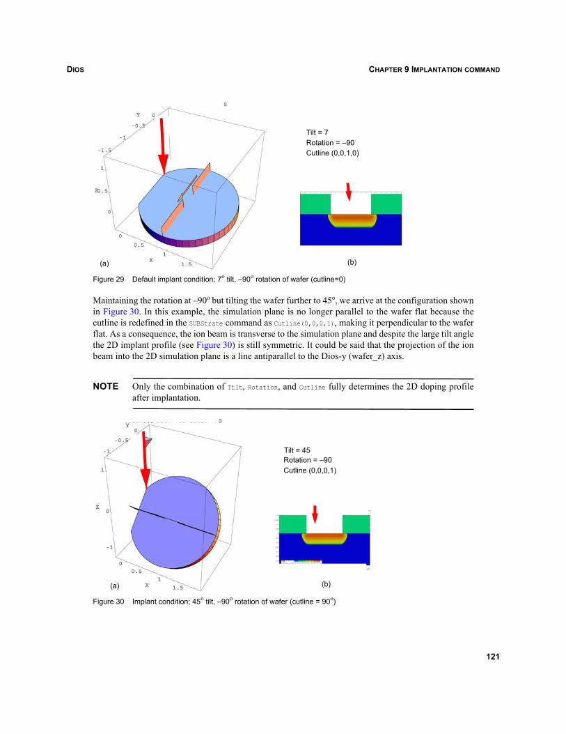
DIOS CHAPTER 9 IMPLANTATION COMMAND
Figure 29 Default implant condition; 7o tilt, –90o rotation of wafer (cutline=0)
Maintaining the rotation at –90o but tilting the wafer further to 45o, we arrive at the configuration shownin Figure 30. In this example, the simulation plane is no longer parallel to the wafer flat because thecutline is redefined in the SUBStrate command as Cutline(0,0,0,1), making it perpendicular to the waferflat. As a consequence, the ion beam is transverse to the simulation plane and despite the large tilt anglethe 2D implant profile (see Figure 30) is still symmetric. It could be said that the projection of the ionbeam into the 2D simulation plane is a line antiparallel to the Dios-y (wafer_z) axis.
NOTE Only the combination of Tilt, Rotation, and Cutline fully determines the 2D doping profileafter implantation.
Figure 30 Implant condition; 45o tilt, –90o rotation of wafer (cutline = 90o)
(b)
Tilt = 7Rotation = –90Cutline (0,0,1,0)
(a)
(a)
Tilt = 45Rotation = –90Cutline (0,0,0,1)
(b)
121
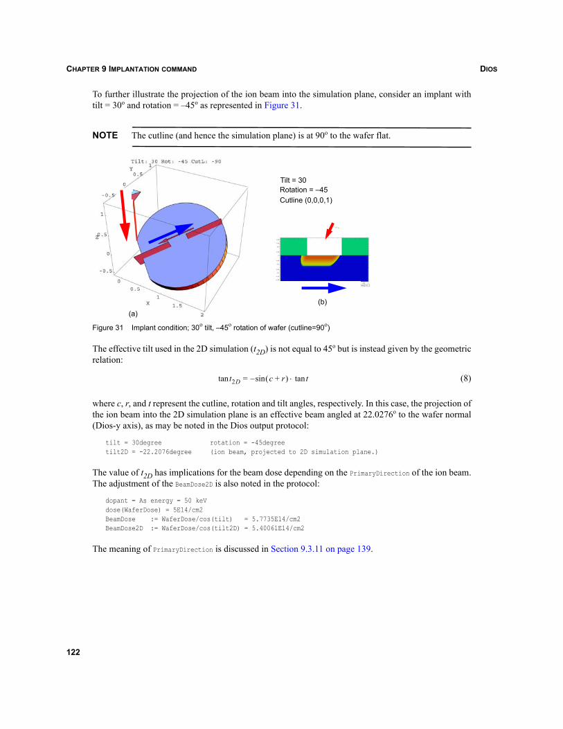
DIOSCHAPTER 9 IMPLANTATION COMMAND
To further illustrate the projection of the ion beam into the simulation plane, consider an implant withtilt = 30o and rotation = –45o as represented in Figure 31.
NOTE The cutline (and hence the simulation plane) is at 90o to the wafer flat.
Figure 31 Implant condition; 30o tilt, –45o rotation of wafer (cutline=90o)
The effective tilt used in the 2D simulation (t2D) is not equal to 45o but is instead given by the geometricrelation:
(8)
where c, r, and t represent the cutline, rotation and tilt angles, respectively. In this case, the projection ofthe ion beam into the 2D simulation plane is an effective beam angled at 22.0276o to the wafer normal(Dios-y axis), as may be noted in the Dios output protocol:
tilt = 30degree rotation = -45degreetilt2D = -22.2076degree (ion beam, projected to 2D simulation plane.)
The value of t2D has implications for the beam dose depending on the PrimaryDirection of the ion beam.The adjustment of the BeamDose2D is also noted in the protocol:
dopant = As energy = 50 keVdose(WaferDose) = 5E14/cm2BeamDose := WaferDose/cos(tilt) = 5.7735E14/cm2BeamDose2D := WaferDose/cos(tilt2D) = 5.40061E14/cm2
The meaning of PrimaryDirection is discussed in Section 9.3.11 on page 139.
Tilt = 30Rotation = –45Cutline (0,0,0,1)
(b)(a)
t2Dtan c r+( )sin–= ttan⋅
122
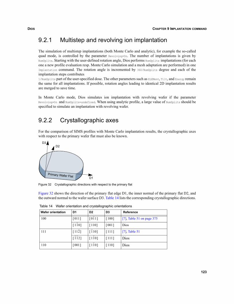
DIOS CHAPTER 9 IMPLANTATION COMMAND
9.2.1 Multistep and revolving ion implantation
The simulation of multistep implantations (both Monte Carlo and analytic), for example the so-calledquad mode, is controlled by the parameter Revolving=On. The number of implantations is given byNumSplits. Starting with the user-defined rotation angle, Dios performs NumSplits implantations (for eachone a new profile evaluation resp. Monte Carlo simulation and a mesh adaptation are performed) in oneImplantation command. The rotation angle is incremented by 360/NumSplits degree and each of theimplantation steps contributes 1/NumSplits part of the user-specified dose. The other parameters such as ELEMent, Tilt, and Energy remainthe same for all implantations. If possible, rotation angles leading to identical 2D implantation resultsare merged to save time.
In Monte Carlo mode, Dios simulates ion implantation with revolving wafer if the parameterRevolving=On and NumSplits=undefined. When using analytic profile, a large value of NumSplits should bespecified to simulate an implantation with revolving wafer.
9.2.2 Crystallographic axes
For the comparison of SIMS profiles with Monte Carlo implantation results, the crystallographic axeswith respect to the primary wafer flat must also be known.
Figure 32 Crystallographic directions with respect to the primary flat
Figure 32 shows the direction of the primary flat edge D1, the inner normal of the primary flat D2, andthe outward normal to the wafer surface D3. Table 14 lists the corresponding crystallographic directions.
Table 14 Wafer orientation and crystallographic orientations
Wafer orientation D1 D2 D3 Reference
[7], Table 51 on page 375
Dios
[7], Table 51
Dios
Dios
D1
D3D2
Primary Wafer Flat
100 011[ ] 011[ ] 100[ ]
110[ ] 110[ ] 001[ ]
111 112[ ] 110[ ] 111[ ]
112[ ] 110[ ] 111[ ]
110 001[ ] 110[ ] 110[ ]
123
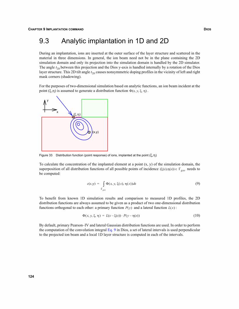
DIOSCHAPTER 9 IMPLANTATION COMMAND
9.3 Analytic implantation in 1D and 2DDuring an implantation, ions are inserted at the outer surface of the layer structure and scattered in thematerial in three dimensions. In general, the ion beam need not be in the plane containing the 2Dsimulation domain and only its projection into the simulation domain is handled by the 2D simulator.The angle t2D between this projection and the Dios y-axis is handled internally by a rotation of the Dioslayer structure. This 2D tilt angle t2D causes nonsymmetric doping profiles in the vicinity of left and rightmask corners (shadowing).
For the purposes of two-dimensional simulation based on analytic functions, an ion beam incident at thepoint (ξ,η) is assumed to generate a distribution function .
Figure 33 Distribution function (point response) of ions, implanted at the point (ξ,η)
To calculate the concentration of the implanted element at a point (x, y) of the simulation domain, thesuperposition of all distribution functions of all possible points of incidence needs tobe computed:
(9)
To benefit from known 1D simulation results and comparison to measured 1D profiles, the 2Ddistribution functions are always assumed to be given as a product of two one-dimensional distributionfunctions orthogonal to each other: a primary function and a lateral function :
(10)
By default, primary Pearson–IV and lateral Gaussian distribution functions are used. In order to performthe computation of the convolution integral Eq. 9 in Dios, a set of lateral intervals is used perpendicularto the projected ion beam and a local 1D layer structure is computed in each of the intervals.
Φ x y ξ η, , ,( )
(ξ,η)
x
xx
y
(x,y)
ξ s( ) η s( )( , ) Γgas∈
c x,y( ) Φ x y ξ s( ) η s( ), , ,( ) sdΓgas
∫=
P y( ) L x( )
Φ x y ξ η, , ,( ) L x ξ s( )–( ) P y η s( )–( )⋅=
124
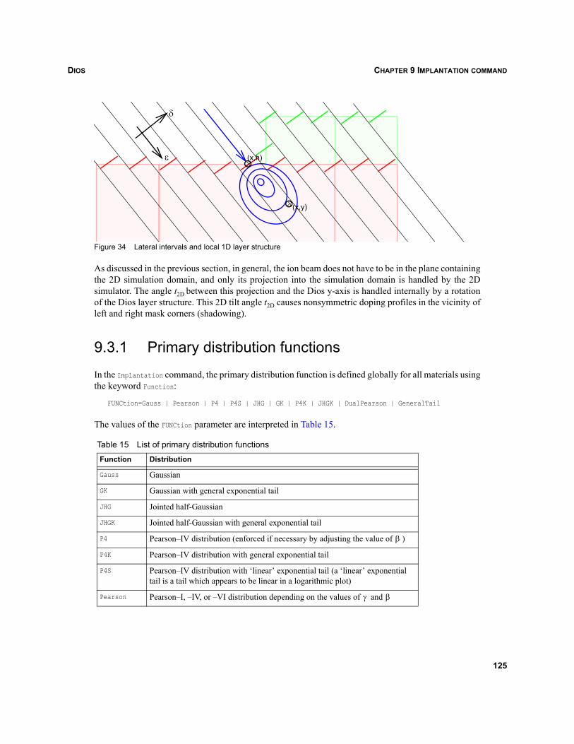
DIOS CHAPTER 9 IMPLANTATION COMMAND
Figure 34 Lateral intervals and local 1D layer structure
As discussed in the previous section, in general, the ion beam does not have to be in the plane containingthe 2D simulation domain, and only its projection into the simulation domain is handled by the 2Dsimulator. The angle t2D between this projection and the Dios y-axis is handled internally by a rotationof the Dios layer structure. This 2D tilt angle t2D causes nonsymmetric doping profiles in the vicinity ofleft and right mask corners (shadowing).
9.3.1 Primary distribution functions
In the Implantation command, the primary distribution function is defined globally for all materials usingthe keyword Function:
FUNCtion=Gauss | Pearson | P4 | P4S | JHG | GK | P4K | JHGK | DualPearson | GeneralTail
The values of the FUNCtion parameter are interpreted in Table 15.
Table 15 List of primary distribution functions
Function Distribution
Gauss Gaussian
GK Gaussian with general exponential tail
JHG Jointed half-Gaussian
JHGK Jointed half-Gaussian with general exponential tail
P4 Pearson–IV distribution (enforced if necessary by adjusting the value of )
P4K Pearson–IV distribution with general exponential tail
P4S Pearson–IV distribution with ‘linear’ exponential tail (a ‘linear’ exponential tail is a tail which appears to be linear in a logarithmic plot)
Pearson Pearson–I, –IV, or –VI distribution depending on the values of and
(x,y)x
ε
δ
(x,h)x
β
γ β
125
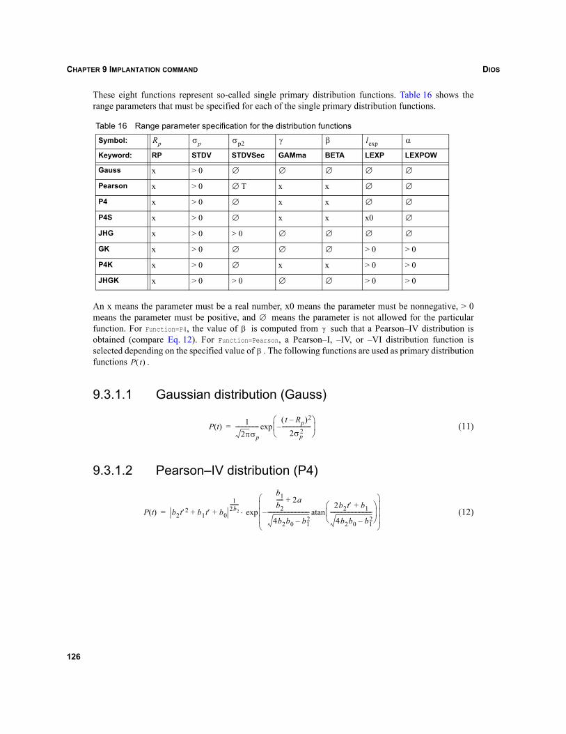
DIOSCHAPTER 9 IMPLANTATION COMMAND
These eight functions represent so-called single primary distribution functions. Table 16 shows therange parameters that must be specified for each of the single primary distribution functions.
An x means the parameter must be a real number, x0 means the parameter must be nonnegative, > 0means the parameter must be positive, and means the parameter is not allowed for the particularfunction. For Function=P4, the value of is computed from such that a Pearson–IV distribution isobtained (compare Eq. 12). For Function=Pearson, a Pearson–I, –IV, or –VI distribution function isselected depending on the specified value of . The following functions are used as primary distributionfunctions .
9.3.1.1 Gaussian distribution (Gauss)
(11)
9.3.1.2 Pearson–IV distribution (P4)
(12)
Table 16 Range parameter specification for the distribution functions
Symbol:
Keyword: RP STDV STDVSec GAMma BETA LEXP LEXPOW
Gauss x > 0
Pearson x > 0 T x x
P4 x > 0 x x
P4S x > 0 x x x0
JHG x > 0 > 0
GK x > 0 > 0 > 0
P4K x > 0 x x > 0 > 0
JHGK x > 0 > 0 > 0 > 0
Rp σp σp2 γ β lexp α
∅ ∅ ∅ ∅ ∅
∅ ∅ ∅
∅ ∅ ∅
∅ ∅
∅ ∅ ∅ ∅
∅ ∅ ∅
∅
∅ ∅
∅β γ
βP t( )
P t( ) 12πσp
-----------------t Rp–( )2
2σp2
---------------------–⎝ ⎠⎜ ⎟⎛ ⎞
exp=
P t( ) b2t′2 b1t′ b0+ +1
2b2--------
b1b2----- 2a+
4b2b0 b12–
------------------------------–2b2t′ b1+
4b2b0 b12–
------------------------------⎝ ⎠⎜ ⎟⎛ ⎞
atan
⎝ ⎠⎜ ⎟⎜ ⎟⎜ ⎟⎛ ⎞
exp⋅=
126
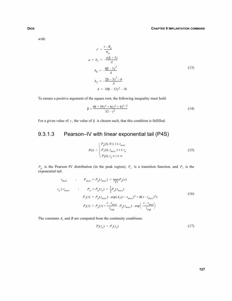
DIOS CHAPTER 9 IMPLANTATION COMMAND
with:
(13)
To ensure a positive argument of the square root, the following inequality must hold:
(14)
For a given value of , the value of is chosen such, that this condition is fulfilled.
9.3.1.3 Pearson–IV with linear exponential tail (P4S)
(15)
is the Pearson–IV distribution (in the peak region), is a transition function, and is theexponential tail.
(16)
The constants A1 and B are computed from the continuity conditions:
(17)
t′t Rp–
σp-------------=
a b1γ β 3+( )
A--------------------–= =
b04β 3γ2–
A---------------------–=
b22β 3γ2– 6–
A------------------------------–=
A 10β 12γ2– 18–=
β 48 39γ2 6 γ2 4+( )3 2⁄++32 γ2–
------------------------------------------------------------->
γ β
P t( )
Pp t( ) 0 t tmax≤ ≤,
Pv t( ) tmax t ta≤ ≤,
Pl t( ) ta t ∞≤ ≤,⎩⎪⎨⎪⎧
=
Pp Pv Pl
tmax : Pmax Pp tmax( ):= Pp t( )t∀
max=
ta tmax≥ : Pa Pp ta( ):= 12---Pp tmax( )=
Pv t( ) Pp tmax( ) A1 t tmax–( )2 B t tmax–( )3+( )exp⋅=
Pl t( ) Pp t( )t tmax–
lexp------------------ Pp tmax( )
t tmax–lexp
------------------–⎝ ⎠⎛ ⎞exp⋅⋅+=
Pl ta( ) Pv ta( )=
127
DIOSCHAPTER 9 IMPLANTATION COMMAND
and:
(18)
NOTE Due to the added tail, the modified distribution function has other than the listed moments.However, the hard-coded lookup tables were computed for amorphous target materials onlyand the added tail accounts for channeling in crystalline material. Be careful when using theexponential tail for implantation with large tilt angles. The lexp fit was performed for standard7o tilt and does not apply for large tilt angles.
9.3.1.4 Pearson distribution
A Pearson–I, Pearson–IV, or Pearson–VI distribution is chosen, depending on the parameters:
(19)
The parameters y1, y2, α1, and α2 are computed from the higher order moments γ and β. The selection ofthe particular distribution function is done according to the sign of y1 and y2. For a given lookup valueof γ, the default value of β is defined from the Biersack Finck parabola. This curve was modified to givealways a valid Pearson–I, Pearson–IV, or Pearson–VI distribution.
9.3.1.5 Jointed half-Gaussian distribution (JHG)
(20)
tdd Pl t( ) ta td
d Pv t( ) taP′a=:=
A1
3Pa
Pmax------------ln
ta tmax–( )2----------------------------
P′aPa ta tmax–( )--------------------------------–=
B2
PaPmax------------ln–
ta tmax–( )3----------------------------
P′a
Pa ta tmax–( )2----------------------------------+=
P t( ) t′ y1– α1 t′ y2– α2 , with t′t Rp–
σp-------------= =
P t( )
n0t Rp–( )2
2σp2
---------------------–⎝ ⎠⎜ ⎟⎛ ⎞
exp t Rp≤,
n0t Rp–( )2
2σp22
---------------------–⎝ ⎠⎜ ⎟⎛ ⎞
exp Rp t<,
⎩⎪⎪⎪⎨⎪⎪⎪⎧
=
128
DIOS CHAPTER 9 IMPLANTATION COMMAND
The norm of the function on the positive real axis is:
(21)
for .
9.3.1.6 Gaussian distribution with general exponential tail (GK)
(22)
The constant is chosen such that the function is continuous at . is the reciprocal value ofthe norm of the function on the positive real axis. The other two functions with general exponential tail(JHGK, P4K) are built up in exactly the same way [54] taking into account the correct position of the peakvalue and the peak value itself in front of the tail function and, of course, replacing the Gaussian by thejointed half-Gaussian resp. by the Pearson–IV distribution.
9.3.2 Dual primary distribution functions
For implantations into crystalline materials, it is often important to take ion channeling into account. Inanalytic implant simulations, this is done by considering the profile to have two components; the firstcomponent representing the profile of ions, which do not channel (this we may call the ‘amorphous’profile) and the second component representing the channeled ions which form the characteristic tail inthe distribution (the ‘channeling’ profile).
A dual primary distribution function is obtained by selecting two primary distribution functions. In theImplantation command the primary distribution function can be defined globally for all materials usingthe keyword Function:
FUNCtion=Gauss | Pearson | P4 | P4S | JHG | GK | P4K | JHGK | DualPearson | GeneralTail
Such dual primary distribution functions can be specified globally in the Implantation statement by, forexample, Function=(JHG,JHGK) or for a particular material in the material record: Si(Function=P4,Function2=P4K). DualPearson and GeneralTail are shortcuts for dual primary distribution functions:DualPearson is interpreted as (P4,P4) and GeneralTail as (P4,P4K).
Examples for the specification of dual analytic primary ion distribution functions:
Implantation(Element=b,Energy=120,Dose=1e12,Function=DualPearson)Implantation(Element=b,Energy=120,Dose=1e12,Function(JHG,JHGK))Implantation(Element=b,Energy=120,Dose=1e12,Si(Function=P4,Function2=P4K))
1n0----- π
2--- σperf
Rp
2σp
-------------⎝ ⎠⎜ ⎟⎛ ⎞
σp2+⎝ ⎠⎜ ⎟⎛ ⎞
=
Rp 0>
P t( )
n0
2πσp
-----------------t Rp–( )2
2σp2
---------------------–⎝ ⎠⎜ ⎟⎛ ⎞
exp t Rp σp+≤,
n0κ 12π σp
-----------------t Rp–( )2
2σp2
---------------------–⎝ ⎠⎜ ⎟⎛ ⎞
exp 12π σp
-----------------t Rp–lexp
-------------⎝ ⎠⎛ ⎞
α–⎝ ⎠
⎛ ⎞exp⋅+⎝ ⎠⎜ ⎟⎛ ⎞
⋅ Rp σp+ t<,
⎩⎪⎪⎪⎨⎪⎪⎪⎧
=
κ Rp σp+ n0
129
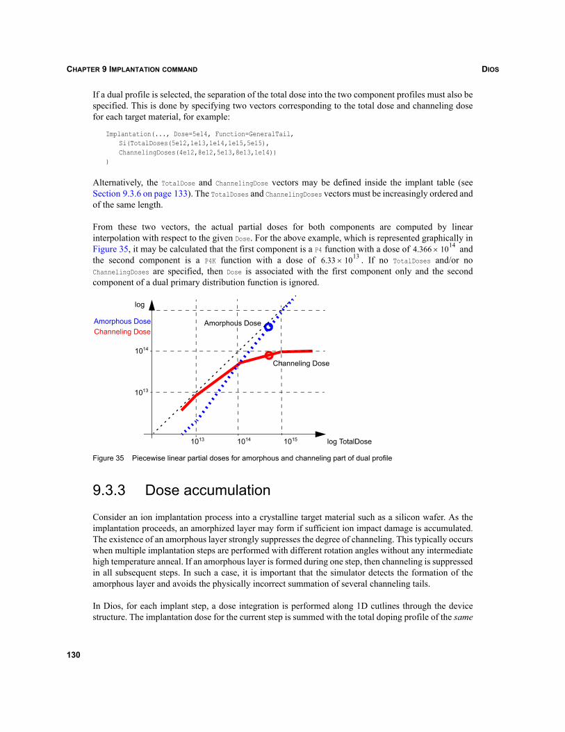
DIOSCHAPTER 9 IMPLANTATION COMMAND
If a dual profile is selected, the separation of the total dose into the two component profiles must also bespecified. This is done by specifying two vectors corresponding to the total dose and channeling dosefor each target material, for example:
Implantation(..., Dose=5e14, Function=GeneralTail,Si(TotalDoses(5e12,1e13,1e14,1e15,5e15),ChannelingDoses(4e12,8e12,5e13,8e13,1e14))
)
Alternatively, the TotalDose and ChannelingDose vectors may be defined inside the implant table (seeSection 9.3.6 on page 133). The TotalDoses and ChannelingDoses vectors must be increasingly ordered andof the same length.
From these two vectors, the actual partial doses for both components are computed by linearinterpolation with respect to the given Dose. For the above example, which is represented graphically inFigure 35, it may be calculated that the first component is a P4 function with a dose of andthe second component is a P4K function with a dose of . If no TotalDoses and/or noChannelingDoses are specified, then Dose is associated with the first component only and the secondcomponent of a dual primary distribution function is ignored.
Figure 35 Piecewise linear partial doses for amorphous and channeling part of dual profile
9.3.3 Dose accumulation
Consider an ion implantation process into a crystalline target material such as a silicon wafer. As theimplantation proceeds, an amorphized layer may form if sufficient ion impact damage is accumulated.The existence of an amorphous layer strongly suppresses the degree of channeling. This typically occurswhen multiple implantation steps are performed with different rotation angles without any intermediatehigh temperature anneal. If an amorphous layer is formed during one step, then channeling is suppressedin all subsequent steps. In such a case, it is important that the simulator detects the formation of theamorphous layer and avoids the physically incorrect summation of several channeling tails.
In Dios, for each implant step, a dose integration is performed along 1D cutlines through the devicestructure. The implantation dose for the current step is summed with the total doping profile of the same
4.366 1014×6.33 1013×
1013 1014 1015 log TotalDose
Channeling Dose
Amorphous Dose
log
Amorphous DoseChanneling Dose
1013
1014
130
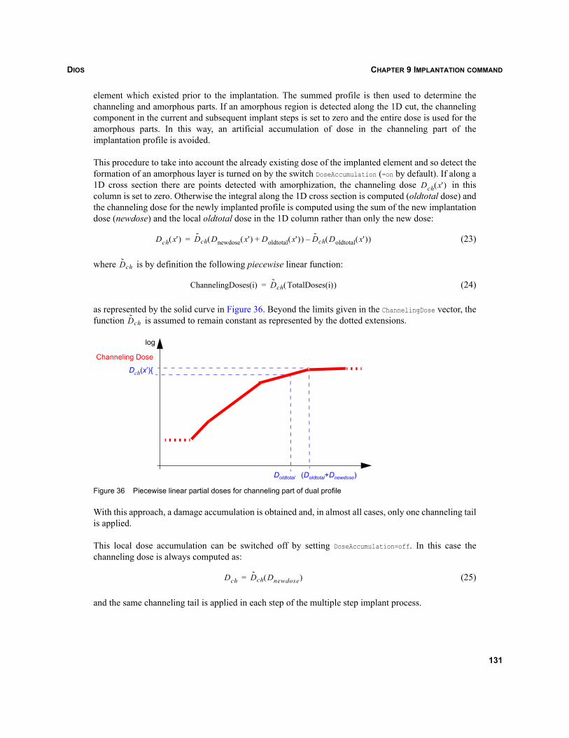
DIOS CHAPTER 9 IMPLANTATION COMMAND
element which existed prior to the implantation. The summed profile is then used to determine thechanneling and amorphous parts. If an amorphous region is detected along the 1D cut, the channelingcomponent in the current and subsequent implant steps is set to zero and the entire dose is used for theamorphous parts. In this way, an artificial accumulation of dose in the channeling part of theimplantation profile is avoided.
This procedure to take into account the already existing dose of the implanted element and so detect theformation of an amorphous layer is turned on by the switch DoseAccumulation (=on by default). If along a1D cross section there are points detected with amorphization, the channeling dose in thiscolumn is set to zero. Otherwise the integral along the 1D cross section is computed (oldtotal dose) andthe channeling dose for the newly implanted profile is computed using the sum of the new implantationdose (newdose) and the local oldtotal dose in the 1D column rather than only the new dose:
(23)
where is by definition the following piecewise linear function:
(24)
as represented by the solid curve in Figure 36. Beyond the limits given in the ChannelingDose vector, thefunction is assumed to remain constant as represented by the dotted extensions.
Figure 36 Piecewise linear partial doses for channeling part of dual profile
With this approach, a damage accumulation is obtained and, in almost all cases, only one channeling tailis applied.
This local dose accumulation can be switched off by setting DoseAccumulation=off. In this case thechanneling dose is always computed as:
(25)
and the same channeling tail is applied in each step of the multiple step implant process.
Dch x'( )
Dch x'( ) Dch Dnewdose x'( ) Doldtotal x'( )+( ) Dch Doldtotal x'( )( )–=
Dch
ChannelingDoses(i) Dch TotalDoses(i)( )=
Dch
Doldtotal (Doldtotal+Dnewdose)
log
Channeling Dose
Dch(x’){
Dch Dch Dnewdose( )=
131
DIOSCHAPTER 9 IMPLANTATION COMMAND
NOTE The described entire integration and accumulation is relevant only for the case of dualprimary functions, since for a single primary function the full implantation dose is alwaysused.
9.3.4 Lateral straggle
The lateral straggling in the distribution of implanted ions is specified by defining a lateral distributionfunction; Lateral=Gaussian | Pearson in combination with a characteristic length parameter Stdvl ( ).By default, the lateral distribution, L(t), is Gaussian:
(26)
If a Pearson–I distribution is selected instead, the user must define an exponent k:
(27)
Alternatively, depth-dependent lateral straggling can be switched on using the flag (DepthDependent=1) fora given target material. Then, the lateral straggle is specified by the vector Lateral/Vertical
( ). For example, for an implant into silicon:
Implantation(..., DepthDependent=1,Si(Lateral/Vertical(1.0, 1.02, 0.3, 0.8, 9.1)))
The vector contains five parameters per material that govern the computation of the lateral stragglingdependence on the depth in the wafer according to:
(28)
9.3.5 Internal implant tables
The moments of the distribution functions , , , , and for each of the materials are chosenby default from a hard-coded internal lookup table. The values are selected according to implantationenergy [keV], implanted element ELEMent and material. If Printout=On is specified, the internal lookuptable is written to a file. The file name can be specified as Table="filename" (default "dios_impl.tab"). Ifa file with the name "filename" exists already, a warning is given and the existing file remains unchanged.
By default, primary Pearson–IV distributions (P4) and lateral Gaussian distributions are used. Forarsenic, phosphorus, antimony, gallium, indium, aluminum, and germanium, the Gibbons tables [14] are
σl
L t( ) 12π σl
---------------- t2
2σl2
---------–⎝ ⎠⎜ ⎟⎛ ⎞
exp=
L t( ) tσl-----⎝ ⎠
⎛ ⎞ k=
p1 p2 … p5,, ,
y
σL σpmax 0.01
p1p2yRp-------- p3+⎝ ⎠
⎛ ⎞⎝ ⎠⎜ ⎟⎛ ⎞
exp p1p4yRp-------- p5+⎝ ⎠
⎛ ⎞⎝ ⎠⎜ ⎟⎛ ⎞
exp+⎝⎜⎛
log⎠⎟⎞
p1--------------------------------------------------------------------------------------------------------------------,
⎝ ⎠⎜ ⎟⎜ ⎟⎜ ⎟⎜ ⎟⎜ ⎟⎛ ⎞
=
Rp σp γ lexp σL
132
DIOS CHAPTER 9 IMPLANTATION COMMAND
used. The data for boron has been obtained from experimental values fitted with the 1D simulatorTESIM-4 [12] and from literature [53]. The values for energies MeV are taken from the literature[5]. The moments of the distribution functions can be defined explicitly for each of the materials. If anyof the parameters RP, STDV, STDVSec, GAMma, BETA, LEXP, LEXPOW, and STDVL is specified (for any of thematerials), it is assumed that the user is supplying data fitted to experiments and no rescaling of and
is performed for any of the materials (see Section 9.3.11.2 on page 140).
For boron in Si and PO, an exponentially decreasing tail is added to the primary distribution function torepresent ion channeling in the crystalline material. The channeling tail starts at half of the maximumvalue of the primary distribution and the internal default for its characteristic length can be redefinedby the user. The list of range parameters, used models, and dose values is always displayed and printedinto the protocol.
BF2 can be specified as an implantation ‘element.’ If an external implant data lookup table is providedfor BF2, the appropriate parameters from that table will be used. If only a table for boron is available, asfor example in the internal lookup table, the implantation energy is reduced internally according to theatomic masses of the boron and the two fluorine ions: . The range parametersare then obtained by looking up the reduced value in the boron table. Except for this change of theenergy, BF2 is treated as boron and the fluorine is always neglected.
9.3.6 External implant tables
As an alternative to using the internal implant tables, the range parameters and dose information can beread from an external file. This is performed if a file name is specified as Table="filename". The file namecan also be prescribed by the environment variable IMPLANT_TABLE. If the range parameters for differentmaterials need to be stored in different files, the file names must be specified per material, for example,as Implantation(Si(Table='filename'...). The file names can be specified with an absolute or a relativepath. Otherwise, files are searched first in the current working directory. If not found there, Dios tries toopen the file in the directory defined by the environment variable $DIOS_LIB and, if not found there, in$STROOT_LIB/dioslib/. The environment symbol DIOS_LIB can be defined by the Dios user; theenvironment symbol STROOT_LIB is reserved for the default setup of all Synopsys tools.
NOTE Dios uses polynomial interpolation when processing the internal hard-coded rangeparameters. For data from external table lookup files, linear interpolation is used (even if thefile copy of the internal table is used).
The file format of the implantation data file is rather general and allows dependencies on energy, dose,tilt, rotation and scattering oxide thickness to be described. It allows the eight types of primary iondistribution functions (Gaussian, Pearson, Pearson–IV, Pearson–IV with linear exponential tail, jointedhalf-Gaussian, and Gaussian, Pearson–IV, jointed half-Gaussian with general exponential tail) to bedescribed and depth-dependent lateral straggling to be included. The format of the table entries is:
#1. Block: 8 numbers in 1 rowDatexnameMaterial DatexnameDopant oxideThickness Rotation Tilt\ Energy NumberOfFunction NumberOfDoses#2. Block: NumberOfFunctions rowsRP STDV STDVSec GAMMA BETA LEXP LEXPOW
1≥
Rplexp
lexp
Eintern Einput 4.4545⁄=
133
DIOSCHAPTER 9 IMPLANTATION COMMAND
RP STDV STDVSec GAMma BETA LEXP LEXPOW#3. Block: NumberOfDoses rowsTotalDose ChannelingDoseTotalDose ChannelingDose...TotalDose ChannelingDose#4. Block: 1 rowp1 p2 p3 p4 p5
Lines with a # in the first column are treated as comment lines. Missing or incomplete blocks are notproperly read when the file is parsed; in this case, Dios switches back to the internal lookup table. Onedata entry consists of four blocks or groups of lines.
The first block contains the datex name (see Section 12.2 on page 284) of the material and dopant, theoxide thickness, rotation angle, tilt angle, and energy of the data entry. For BF2, the string BF2 is used,since no datex name is defined. In the case of a BF2 implant table, the user-defined energy of the BF2 ionis used for the lookup. If no BF2 table but a boron table is found, the energy share of the boron ion isused for the lookup of data.
NumberOfFunctions defines the number of components of the primary distribution function, andNumberOfDoses defines the number of pairs, each of which consists of a total dose and a correspondingchanneling dose. All doses are expected to be positive.
The second block contains the range parameters for all the components of the primary distributionfunction. Parameters that by definition do not exist for the function, which the set describes, should beset equal to zero. Dios recognizes from the read parameter values the intended function or tries to buildup a simpler primary function component if the set itself does not fit into any of the eight primarydistribution functions listed above. In the latter case, a warning message is given.
The third block contains the dose information of the entry increasingly ordered and the fourth block theparameters for the depth-dependent lateral straggling. Concerning the order of the data entries in the datafile, the following assumption should be fulfilled: the entries are increasingly ordered with respect toOxideThickness, Rotation, Tilt, Energy, such that the values for the various energies (but the same otherthree parameters) follow each other. All data entries to the same material dopant pair should follow eachother with no interruption by entries to another material dopant pair. The oxide thickness and the rangeparameters with the physical unit ‘length’ should be given in microns. The angles are given in degree.The energy values must be specified in keV. No unit must be specified in the tables.
9.3.7 University of Texas implant tables
As an alternative to the internal tables, Dios allows the use of a set of external tables, which areconverted from the University of Texas Range Parameter tables (also known as Al Tasch tables). Thesetables are distributed with Dios and are located in $STROOT_LIB/dioslib/.
134
DIOS CHAPTER 9 IMPLANTATION COMMAND
These files can be loaded as external tables as described in Section 9.3.6 on page 133, that is, using thecommand IMPLantation:(Si:(Table='filename')). The files contain lookup tables for double Pearson–IVdistributions for crystalline silicon. The following files are available:
UT_As_impl.tab Arsenic (0.5–180 keV)
UT_B_impl.tab Boron (0.5–80 keV)
UT_B_SO_impl.tab Boron (15–80 keV, screen oxide: 1.5–40 nm)
UT_BF2_impl.tab BF2 (0.5–65 keV)
UT_P_impl.tab Phosphorus (15–180 keV)
The valid range for the tilt is 0–10o and for the rotation, 0–45o. All tables except UT_B_SO_impl.tab arecollected in one table, which is named UT_impl.tab. In addition, UT_B_SO_impl.tab provides oxidethickness–dependent data for boron.
NOTE These tables are not fully compatible with the original data. The new tables result from anonlinear fit of 5–7 dose-dependent measurements for each table entry in the originalUniversity of Texas table.
In addition, in some cases, Beta and Beta2 were corrected in order to provide Dios-compatible data.Expect deviations from the original profiles in the tails below densities of 1015 cm–3.
9.3.8 Implantation tables based on Crystal-TRIM
There are implantation tables with Pearson parameters for arsenic, boron, BF2, indium, phosphorus,antimony, and germanium, which are located in $STROOT_LIB/dioslib/. They cover the materials silicon,polysilicon, oxide, and nitride. For silicon, dual Pearson functions are used with parameters dependingon energy, tilt angle (0–60o), dose, and oxide thickness. For the other materials, single Pearson functionsare used with parameters depending on implantation energy and tilt.
All entries are based on optimized fits to Monte Carlo Crystal-TRIM simulations, which have beencalibrated with SIMS profiles and performed with a high number of particles. Each table covers oneimplantation species and a limited dose range. Table 17 lists the available tables.
Table 17 Tables for analytic implantation
Implantation species
Energy range [keV]
Low dose Medium dose High dose
As 0.5–400 As_1e12-5e13.tab As_1e13-8e14.tab As_2e14-6e15.tab
B 0.2–480 B_1e12-4e13_2003.tabB_1e12-4e13.tab
B_1e13-6e14_2003.tabB_1e13-6e14.tab
B_16e13-8e15_2003.tabB_16e13-8e15.tab
BF2 0.5–400 BF2_1e12-5e13.tab BF2_1e13-8e14.tab BF2_2e14-6e15.tab
In 1.0–400 In_1e12-4e13.tab In_1e13-6e14.tab In_16e13-8e15.tab
135
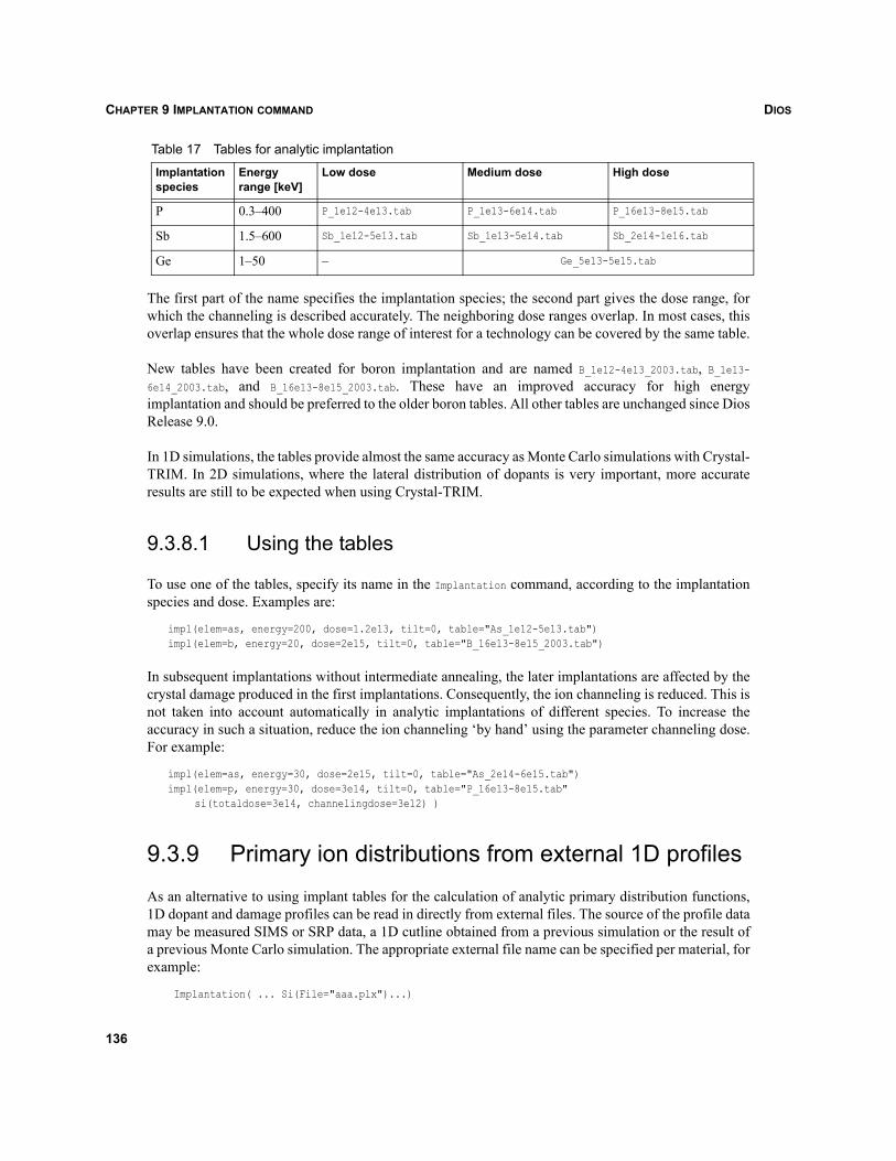
DIOSCHAPTER 9 IMPLANTATION COMMAND
The first part of the name specifies the implantation species; the second part gives the dose range, forwhich the channeling is described accurately. The neighboring dose ranges overlap. In most cases, thisoverlap ensures that the whole dose range of interest for a technology can be covered by the same table.
New tables have been created for boron implantation and are named B_1e12-4e13_2003.tab, B_1e13-6e14_2003.tab, and B_16e13-8e15_2003.tab. These have an improved accuracy for high energyimplantation and should be preferred to the older boron tables. All other tables are unchanged since DiosRelease 9.0.
In 1D simulations, the tables provide almost the same accuracy as Monte Carlo simulations with Crystal-TRIM. In 2D simulations, where the lateral distribution of dopants is very important, more accurateresults are still to be expected when using Crystal-TRIM.
9.3.8.1 Using the tables
To use one of the tables, specify its name in the Implantation command, according to the implantationspecies and dose. Examples are:
impl(elem=as, energy=200, dose=1.2e13, tilt=0, table="As_1e12-5e13.tab")impl(elem=b, energy=20, dose=2e15, tilt=0, table="B_16e13-8e15_2003.tab")
In subsequent implantations without intermediate annealing, the later implantations are affected by thecrystal damage produced in the first implantations. Consequently, the ion channeling is reduced. This isnot taken into account automatically in analytic implantations of different species. To increase theaccuracy in such a situation, reduce the ion channeling ‘by hand’ using the parameter channeling dose.For example:
impl(elem=as, energy=30, dose=2e15, tilt=0, table="As_2e14-6e15.tab")impl(elem=p, energy=30, dose=3e14, tilt=0, table="P_16e13-8e15.tab"
si(totaldose=3e14, channelingdose=3e12) )
9.3.9 Primary ion distributions from external 1D profiles
As an alternative to using implant tables for the calculation of analytic primary distribution functions,1D dopant and damage profiles can be read in directly from external files. The source of the profile datamay be measured SIMS or SRP data, a 1D cutline obtained from a previous simulation or the result ofa previous Monte Carlo simulation. The appropriate external file name can be specified per material, forexample:
Implantation( ... Si(File="aaa.plx")...)
P 0.3–400 P_1e12-4e13.tab P_1e13-6e14.tab P_16e13-8e15.tab
Sb 1.5–600 Sb_1e12-5e13.tab Sb_1e13-5e14.tab Sb_2e14-1e16.tab
Ge 1–50 – Ge_5e13-5e15.tab
Table 17 Tables for analytic implantation
Implantation species
Energy range [keV]
Low dose Medium dose High dose
136
DIOS CHAPTER 9 IMPLANTATION COMMAND
The file format is simple: a dataset name enclosed in double quotation marks (this can be any Dios orDATEX species name or the string ‘doping’). The line with the dataset name is followed by lines eachcontaining a pair of depth [nm] and concentration [cm–3] values.
Several datasets are separated by an empty line:
"ArsenicConcentration"0 2e2130 1.5e21100 1e18200 1e10
"Amorphization"0 1.15e2230 1.15e2235 1e10
If the parameter Damage is specified in the Implantation command and the material is silicon orpolysilicon, the specified file is also searched for a second dataset, defining the implantation damage.The name for the second dataset is Damage or any of the following Dios dataset names: Amorphization,ITotal, VTotal, or their corresponding DATEX counterparts. The first dataset with any of these names isused and any further datasets with these names are ignored. If no dataset for the damage can be found inthe file, a warning is given and the damage is defined according to the value of the parameter Damageeither from the doping profile (Damage=+1) or from the analytic Hobler model.
NOTE If the 1D profiles are given in micrometer instead of nanometer, the parameter Factor=1 mustbe specified.
If the parameter Function=1DMC is specified and if the specified files cannot be read, or do not contain datafor the doping profile, an intermediate 1D Monte Carlo simulation is started to create the file (for eachof the materials with specified file name). If Function=1DMC and no file names are given per material, a1D Monte Carlo simulation is started only for crystalline silicon.
If no external 1D files are given or computed for a material, analytic profiles are used. The combinationof data from files and analytic profiles is performed with the usual dose matching approach(Matching=Dose). The lateral integration and lateral distribution functions are identical if data files oranalytic profiles are used.
9.3.10 Dose-matching in layered 1D structures
From 1D measurements (or from the implant tables), the 1D profiles for large area and thickhomogeneous layers of a given material can be determined, the moments of the distribution function canbe computed, and a single or dual distribution function for the single material can be defined. However,the calculation of 1D profiles for multilayered 1D targets requires an algorithm to combine these initialresults obtained for homogeneous materials to handle arbitrary combinations of materials and layerthicknesses.
137
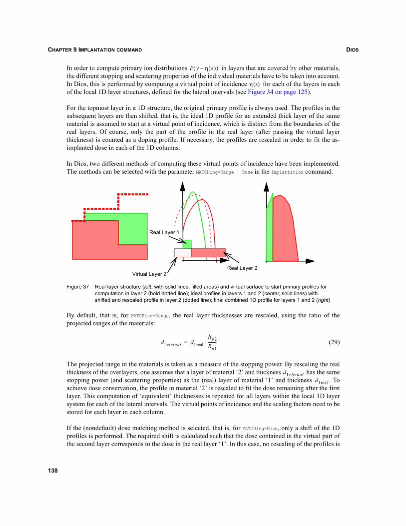
DIOSCHAPTER 9 IMPLANTATION COMMAND
In order to compute primary ion distributions in layers that are covered by other materials,the different stopping and scattering properties of the individual materials have to be taken into account.In Dios, this is performed by computing a virtual point of incidence for each of the layers in eachof the local 1D layer structures, defined for the lateral intervals (see Figure 34 on page 125).
For the topmost layer in a 1D structure, the original primary profile is always used. The profiles in thesubsequent layers are then shifted, that is, the ideal 1D profile for an extended thick layer of the samematerial is assumed to start at a virtual point of incidence, which is distinct from the boundaries of thereal layers. Of course, only the part of the profile in the real layer (after passing the virtual layerthickness) is counted as a doping profile. If necessary, the profiles are rescaled in order to fit the as-implanted dose in each of the 1D columns.
In Dios, two different methods of computing these virtual points of incidence have been implemented.The methods can be selected with the parameter MATCHing=Range | Dose in the Implantation command.
Figure 37 Real layer structure (left, with solid lines, filled areas) and virtual surface to start primary profiles for computation in layer 2 (bold dotted line); ideal profiles in layers 1 and 2 (center, solid lines) with shifted and rescaled profile in layer 2 (dotted line); final combined 1D profile for layers 1 and 2 (right)
By default, that is, for MATCHing=Range, the real layer thicknesses are rescaled, using the ratio of theprojected ranges of the materials:
(29)
The projected range in the materials is taken as a measure of the stopping power. By rescaling the realthickness of the overlayers, one assumes that a layer of material ‘2’ and thickness has the samestopping power (and scattering properties) as the (real) layer of material ‘1’ and thickness . Toachieve dose conservation, the profile in material ‘2’ is rescaled to fit the dose remaining after the firstlayer. This computation of ‘equivalent’ thicknesses is repeated for all layers within the local 1D layersystem for each of the lateral intervals. The virtual points of incidence and the scaling factors need to bestored for each layer in each column.
If the (nondefault) dose matching method is selected, that is, for MATCHing=Dose, only a shift of the 1Dprofiles is performed. The required shift is calculated such that the dose contained in the virtual part ofthe second layer corresponds to the dose in the real layer ‘1’. In this case, no rescaling of the profiles is
P y η s( )–( )
η(s)
Real Layer 2Virtual Layer 2
Real Layer 1
d1virtual d1realRp2Rp1--------⋅=
d1virtuald1real
138
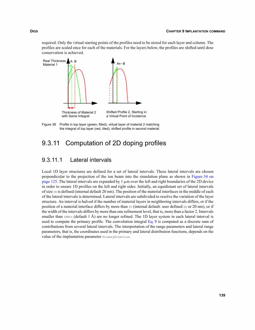
DIOS CHAPTER 9 IMPLANTATION COMMAND
required. Only the virtual starting points of the profiles need to be stored for each layer and column. Theprofiles are scaled once for each of the materials. For the layers below, the profiles are shifted until doseconservation is achieved.
Figure 38 Profile in top layer (green, filled), virtual layer of material 2 matching the integral of top layer (red, tiled), shifted profile in second material
9.3.11 Computation of 2D doping profiles
9.3.11.1 Lateral intervals
Local 1D layer structures are defined for a set of lateral intervals. These lateral intervals are chosenperpendicular to the projection of the ion beam into the simulation plane as shown in Figure 34 onpage 125. The lateral intervals are expanded by 1 μm over the left and right boundaries of the 2D devicein order to ensure 1D profiles on the left and right sides. Initially, an equidistant set of lateral intervalsof size DX is defined (internal default 20 nm). The position of the material interfaces in the middle of eachof the lateral intervals is determined. Lateral intervals are subdivided to resolve the variation of the layerstructure. An interval is halved if the number of material layers in neighboring intervals differs, or if theposition of a material interface differs by more than DY (internal default: user defined DX or 20 nm), or ifthe width of the intervals differs by more than one refinement level, that is, more than a factor 2. Intervalssmaller than DXMin (default 1 Å) are no longer refined. The 1D layer system in each lateral interval isused to compute the primary profile. The convolution integral Eq. 9 is computed as a discrete sum ofcontributions from several lateral intervals. The interpretation of the range parameters and lateral rangeparameters, that is, the coordinates used in the primary and lateral distribution functions, depends on thevalue of the implantation parameter PrimaryDirection.
Shifted Profile 2, Starting ina Virtual Point of Incidence
A B A←BReal ThicknessMaterial 1
Thickness of Material 2with Same Integral
139
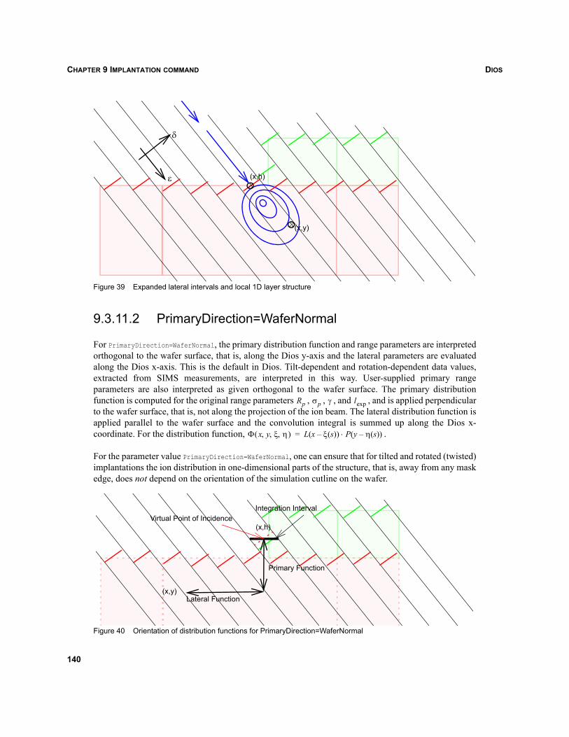
DIOSCHAPTER 9 IMPLANTATION COMMAND
Figure 39 Expanded lateral intervals and local 1D layer structure
9.3.11.2 PrimaryDirection=WaferNormal
For PrimaryDirection=WaferNormal, the primary distribution function and range parameters are interpretedorthogonal to the wafer surface, that is, along the Dios y-axis and the lateral parameters are evaluatedalong the Dios x-axis. This is the default in Dios. Tilt-dependent and rotation-dependent data values,extracted from SIMS measurements, are interpreted in this way. User-supplied primary rangeparameters are also interpreted as given orthogonal to the wafer surface. The primary distributionfunction is computed for the original range parameters , , , and , and is applied perpendicularto the wafer surface, that is, not along the projection of the ion beam. The lateral distribution function isapplied parallel to the wafer surface and the convolution integral is summed up along the Dios x-coordinate. For the distribution function, .
For the parameter value PrimaryDirection=WaferNormal, one can ensure that for tilted and rotated (twisted)implantations the ion distribution in one-dimensional parts of the structure, that is, away from any maskedge, does not depend on the orientation of the simulation cutline on the wafer.
Figure 40 Orientation of distribution functions for PrimaryDirection=WaferNormal
(x,y)x
ε
δ
(x,h)x
Rp σp γ lexp
Φ x y ξ η, , ,( ) L x ξ s( )–( ) P y η s( )–( )⋅=
Primary Function
(x,y)Lateral Function
Integration IntervalVirtual Point of Incidence
(x,h)
140
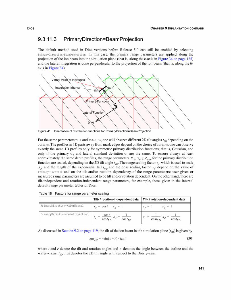
DIOS CHAPTER 9 IMPLANTATION COMMAND
9.3.11.3 PrimaryDirection=BeamProjection
The default method used in Dios versions before Release 5.0 can still be enabled by selectingPrimaryDirection=BeamProjection. In this case, the primary range parameters are applied along theprojection of the ion beam into the simulation plane (that is, along the ε-axis in Figure 34 on page 125)and the lateral integration is done perpendicular to the projection of the ion beam (that is, along the δ-axis in Figure 34).
Figure 41 Orientation of distribution functions for PrimaryDirection=BeamProjection
For the same parameters Tilt and ROTation, one will observe different 2D tilt angles t2D depending on theCUTline. The profiles in 1D parts away from mask edges depend on the choice of CUTline, one can observeexactly the same 1D profiles only for symmetric primary distribution functions, that is, Gaussian, andonly if the primary σp and lateral standard deviation σl are the same. To ensure always at leastapproximately the same depth profiles, the range parameters for the primary distributionfunction are scaled, depending on the 2D tilt angle t2D. The range scaling factor which is used to scale
and the length of the exponential tail lexp and the dose scaling factor depend on the value ofPrimaryDirection and on the tilt and/or rotation dependency of the range parameters: user given ormeasured range parameters are assumed to be tilt and/or rotation dependent. On the other hand, there aretilt-independent and rotation-independent range parameters, for example, those given in the internaldefault range parameter tables of Dios.
As discussed in Section 9.2 on page 119, the tilt of the ion beam in the simulation plane (t2D) is given by:
(30)
where t and r denote the tilt and rotation angles and denotes the angle between the cutline and thewafer-x axis. t2D thus denotes the 2D tilt angle with respect to the Dios y-axis.
Table 18 Factors for range parameter scaling
Tilt- / rotation-independent data Tilt- / rotation-dependent data
PrimaryDirection=WaferNormal
PrimaryDirection=BeamProjection
(x,y)
Integration Interval (x,h)
Virtual Point of Incidence
Lateral Function
Primary Function
R′p σp γ l′exp, , ,sr
Rp sd
sr tcos= sd 1= sr 1= sd 1=
srtcos
t2Dcos----------------= sd
1t2Dcos
----------------= sr1t2Dcos
----------------= sd1t2Dcos
----------------=
t2Dtan c r+( )sin–= ttan⋅
c
141
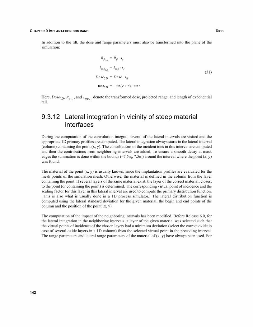
DIOSCHAPTER 9 IMPLANTATION COMMAND
In addition to the tilt, the dose and range parameters must also be transformed into the plane of thesimulation:
(31)
Here, Dose2D, , and denote the transformed dose, projected range, and length of exponentialtail.
9.3.12 Lateral integration in vicinity of steep material interfaces
During the computation of the convolution integral, several of the lateral intervals are visited and theappropriate 1D primary profiles are computed. The lateral integration always starts in the lateral interval(column) containing the point (x, y). The contributions of the incident ions in this interval are computedand then the contributions from neighboring intervals are added. To ensure a smooth decay at maskedges the summation is done within the bounds (–7.5σl, 7.5σl) around the interval where the point (x, y)was found.
The material of the point (x, y) is usually known, since the implantation profiles are evaluated for themesh points of the simulation mesh. Otherwise, the material is defined in the column from the layercontaining the point. If several layers of the same material exist, the layer of the correct material, closestto the point (or containing the point) is determined. The corresponding virtual point of incidence and thescaling factor for this layer in this lateral interval are used to compute the primary distribution function.(This is also what is usually done in a 1D process simulator.) The lateral distribution function iscomputed using the lateral standard deviation for the given material, the begin and end points of thecolumn and the position of the point (x, y).
The computation of the impact of the neighboring intervals has been modified. Before Release 6.0, forthe lateral integration in the neighboring intervals, a layer of the given material was selected such thatthe virtual points of incidence of the chosen layers had a minimum deviation (select the correct oxide incase of several oxide layers in a 1D column) from the selected virtual point in the preceding interval.The range parameters and lateral range parameters of the material of (x, y) have always been used. For
RP2DRP sr⋅=
lexp2Dlexp sr⋅=
Dose2D Dose sd⋅=
t2Dtan c r+( )sin– ttan⋅=
Rp2Dlexp2D
142
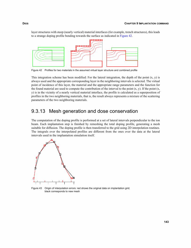
DIOS CHAPTER 9 IMPLANTATION COMMAND
layer structures with steep (nearly vertical) material interfaces (for example, trench structures), this leadsto a strange doping profile bending towards the surface as indicated in Figure 42.
Figure 42 Profiles for two materials in the assumed virtual layer structure and combined profile
This integration scheme has been modified: For the lateral integration, the depth of the point (x, y) isalways used and the appropriate corresponding layer in the neighboring intervals is selected. The virtualpoint of incidence of this layer, the material and the appropriate range parameters and the function forthe found material are used to compute the contribution of the interval to the point (x, y). If the point (x,y) is in the vicinity of a nearly vertical material interface, the profile is calculated as a superposition ofprofiles in the two neighboring materials, that is, the result always represents a mixture of the scatteringparameters of the two neighboring materials.
9.3.13 Mesh generation and dose conservation
The computation of the doping profile is performed at a set of lateral intervals perpendicular to the ionbeam. Each implantation step is finished by remeshing the total doping profile, generating a meshsuitable for diffusion. The doping profile is then transferred to the grid using 2D interpolation routines.The integrals over the interpolated profiles are different from the ones over the data at the lateralintervals used in the implantation simulation itself.
Figure 43 Origin of interpolation errors: red shows the original data on implantation grid; black corresponds to new mesh
143
DIOSCHAPTER 9 IMPLANTATION COMMAND
Dios allows for a rescaling of the as-implanted profile by using the command:
Implantation(FitAsImplantedDose=on)
which is equivalent to the default behavior. The profile is rescaled by a constant factor in order topreserve the implanted dose. Usually, there is a dose loss that results in a rescaling factor greater thanone and an upward shift of the whole profile. This can lead to shifts in the peak value of the profile dueto dose mismatches in regions where the grid is coarse. If the difference in the profiles is too great,rescaling is avoided even with FitAsImplantedDose=on.
9.4 Analytic implantation in 3DAnalytic implantation into 3D structures can be performed using the Imp3D module. There are two waysto load a DF–ISE compatible boundary (.bnd) file for subsequent 3D implantation. An arbitraryboundary file can be loaded before an implantation step using the command:
Load(File=boundary_file.bnd)
Alternatively, a structure without a gas region can be directly specified in the Implantation statement:
Implantation:(Imp3DBoundaryFile=boundary_file.bnd)
The Imp3D code is linked with the 3D mesh generator Mesh, which is integrated in Dios. This allowsthe calculation of 3D doping and point defect profiles combined with adaptive meshing.
The meshing is controlled by loading an external mesh command file before an implantation step isperformed, that is:
Load(File=mesh_command_file.cmd)
Its syntax is the same as for the tool Mesh. In fact, an external Mesh binary can be called instead of usingthe linked-in version via a system call using Replace(Control(MeshCall='mesh -P')) before the firstImplantation command. Here, ‘mesh’ refers to the binary to be called (including appropriate path name).
NOTE The Grid command of Dios and all refinement settings related to the 2D Dios grid have noeffect on the 3D mesh.
Two models to handle multilayered targets are implemented. The default model is the numeric rangematching model as is available in 1D and 2D. It can be switched on using Match=Range. Another method,the method of equivalent atomic stopping (MEAS) [20], is used if Matching=Dose is specified. However,the numeric range scaling model gives better results, especially if thick nonsilicon layers are involved[21]. MEAS may be faster in certain conditions but is not as accurate for thick nonsilicon maskinglayers. A smaller set of the model features is available for the MEAS model, in particular, only the +1model for defects can be used.
The accuracy of the convolution integral calculation can be controlled with two parameters NLatStdDevand NLatDiscPts. These parameters define the local integration (tensor-)grid. The number of points in the
144
DIOS CHAPTER 9 IMPLANTATION COMMAND
grid is (2*NlatDiscPts*NlatStdDev)2. The CPU time is proportional to the number of grid points. To ensurethe accuracy of the convolution integration at all depths, the number of the integration points per meanlateral standard deviation of the implanted impurity NlatDiscPts is set to 5.
The following depth distribution functions are available:
FUNCtion=Gauss|P4|Pearson|P4S|DualPearson
The range parameters can be taken from the internal Dios table or can be loaded externally as in 1D and2D simulations. The depth-dependent lateral straggling of the implanted ion can be simulated in thesame way as in 2D using the parameter record Lateral/Vertical of the Implantation command.
The following damage models are available:
Damage=No|+1|Hobler
These models can be controlled with the same set of parameters as in 1D and 2D simulations.
9.5 Monte Carlo implantationDios allows the atomistic simulation of ballistic processes during ion implantation using the programCrystal-TRIM, which is based on the TRIM (TRansport of Ions in Matter) code [5]. It has beenintegrated with Dios and can be selected with the parameter:
Implantation(FUNCtion=CrystalTrim)
Fundamental implantation parameters like dopant species, implantation energy and dose, the orientationof the ion beam with respect to the crystal axes of the silicon substrate as well as the beam divergencehave to be specified using ELEMent, ENergy, Dose, Tilt, Rotation (or Revolving), and BeamDivergence,respectively.
In most applications, the orientation of the ion beam is constant throughout the implantation process. Ifthe rotation angle is changed during the implantation, Revolving=on has to be specified instead of theRotation parameter. A step-by-step rotation (between 0o and 360o) is considered if the number of stepsis given by the parameter NumSplits. Otherwise, that is, if NumSplits=undefined or 0o, the rotation angle ischanged randomly between 0oand 360o during the implantation. If the implanted ion cannot beprescribed by the ELEMent parameter, it has to be specified by AtomicNumber and AtomicDose. In this case,Dios does not calculate the actual 2D distribution of the implanted ions, but it allows the calculation ofthe implantation damage.
145
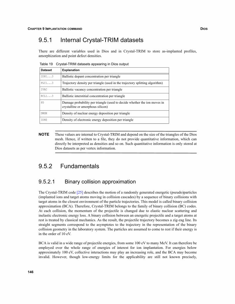
DIOSCHAPTER 9 IMPLANTATION COMMAND
9.5.1 Internal Crystal-TRIM datasets
There are different variables used in Dios and in Crystal-TRIM to store as-implanted profiles,amorphization and point defect densities.
NOTE These values are internal to Crystal-TRIM and depend on the size of the triangles of the Diosmesh. Hence, if written to a file, they do not provide quantitative information, which candirectly be interpreted as densities and so on. Such quantitative information is only stored atDios datasets as per vertex information.
9.5.2 Fundamentals
9.5.2.1 Binary collision approximation
The Crystal-TRIM code [25] describes the motion of a randomly generated energetic (pseudo)particles(implanted ions and target atoms moving in collision cascades) by a sequence of binary collisions withtarget atoms in the closest environment of the particle trajectories. This model is called binary collisionapproximation (BCA). Therefore, Crystal-TRIM belongs to the family of binary collision (BC) codes.At each collision, the momentum of the projectile is changed due to elastic nuclear scattering andinelastic electronic energy loss. A binary collision between an energetic projectile and a target atoms atrest is treated by classical mechanics. As the result, the projectile trajectory becomes a zig-zag line. Itsstraight segments correspond to the asymptotes to the trajectory in the representation of the binarycollision geometry in the laboratory system. The particles are assumed to come to rest if their energy isin the order of 10 eV.
BCA is valid in a wide range of projectile energies, from some 100 eV to many MeV. It can therefore beemployed over the whole range of energies of interest for ion implantation. For energies belowapproximately 100 eV, collective interactions may play an increasing role, and the BCA may becomeinvalid. However, though low-energy limits for the applicability are still not known precisely,
Table 19 Crystal-TRIM datasets appearing in Dios output
Dataset Explanation
ION1...3 Ballistic dopant concentration per triangle
PLC1...3 Trajectory density per triangle (used in the trajectory splitting algorithm)
IVAC Ballistic vacancy concentration per triangle
RCL1...3 Ballistic interstitial concentration per triangle
PD Damage probability per triangle (used to decide whether the ion moves in crystalline or amorphous silicon)
DMGN Density of nuclear energy deposition per triangle
IONS Density of electronic energy deposition per triangle
146
DIOS CHAPTER 9 IMPLANTATION COMMAND
applications of the Crystal-TRIM code to ultra low energy implants led to results that are still sufficientlycorrect. Due to the use of random numbers, Crystal-TRIM is also called Monte Carlo (MC) code. Thismore general term is used in the following text as well.
9.5.2.2 Pseudoparticles
The energetic particles (implanted ions and target atoms moving in collision cascades), which areconsidered in the Crystal-TRIM simulation, are mostly not identical with single ions or atoms butstatistical objects representing several energetic particles or only a fraction of them. Therefore, they arealso called pseudoparticles. This approach enables a considerable increase of the efficiency of the MonteCarlo simulation method, for example, by the application of trajectory splitting and lateral replication(or trajectory transfer) procedures which are described below. The user-defined number of implanted(pseudo)particles is given by Particles (for a more detailed explanation see below).
9.5.2.3 Nuclear collisions and collision cascades
In Crystal-TRIM, a screened Coulombic potential that is valid for most projectile–target combinations,the so-called ZBL potential, is used to treat the elastic scattering of a projectile at a target atom. Thescattering again leads to energy loss of the projectile and energy transfer to the target atom, andconsequently to a change of the direction of motion of the projectile. If the energy transfer to the targetatoms exceeds the so-called displacement threshold (about 15 eV), the target atom can leave its site andbecomes displaced.
Two versions of Crystal-TRIM are available: If the parameter Cascades=off (default) is set, only thetrajectories of the implanted ions are simulated, and the distribution of the vacancies and displaced targetatoms is calculated approximately using the (modified) Kinchin–Pease formula. A full cascadesimulation is performed for Cascades=on. Then, not only the motion of the incident ions but also thetrajectories of energetic target atoms in collision cascades are considered. While both versions yieldcorrect range profiles only the full cascade simulation yields physically correct profiles of ballisticallyproduced vacancies and displaced target atoms. In particular the spatial separation between vacanciesand displaced atoms can only be obtained using this version. However, a full cascade simulation needsmore computational time.
In single-crystalline silicon, the ballistically produced vacancies and the displaced target atoms (recoils)are often identified with the vacancies and interstitials responsible for the transient enhanced diffusion(TED) of dopants. The choice of diffusion model determines whether the full-cascade version ofCrystal-TRIM must be applied or not. All data necessary to process the elastic nuclear scattering areprovided by Crystal-TRIM and Dios.
9.5.2.4 Electronic energy loss
Electronic excitations at a binary collision and between two collisions are described by the inelasticelectronic energy loss of the projectile. It is treated using semi-empirical models. If an energetic particlemoves through single-crystalline and amorphous silicon, a local approach is employed, where theelectronic energy loss depends on the local electronic density in the environment of the projectile. The
147
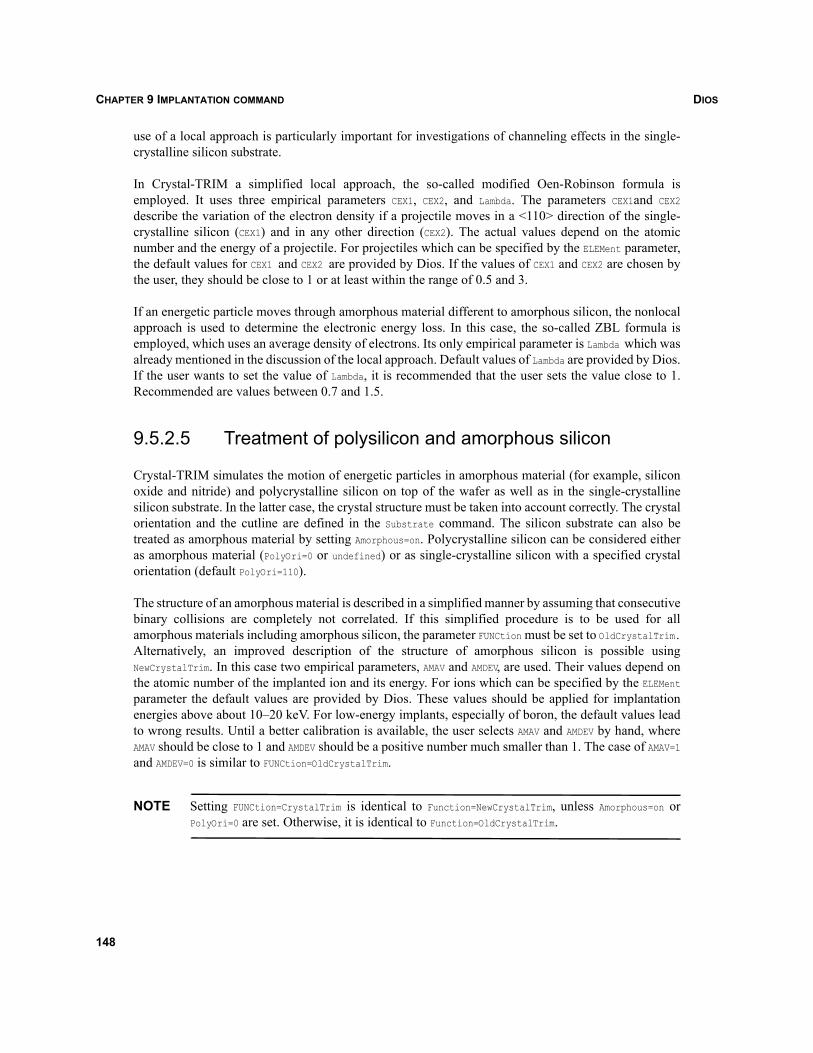
DIOSCHAPTER 9 IMPLANTATION COMMAND
use of a local approach is particularly important for investigations of channeling effects in the single-crystalline silicon substrate.
In Crystal-TRIM a simplified local approach, the so-called modified Oen-Robinson formula isemployed. It uses three empirical parameters CEX1, CEX2, and Lambda. The parameters CEX1and CEX2describe the variation of the electron density if a projectile moves in a <110> direction of the single-crystalline silicon (CEX1) and in any other direction (CEX2). The actual values depend on the atomicnumber and the energy of a projectile. For projectiles which can be specified by the ELEMent parameter,the default values for CEX1 and CEX2 are provided by Dios. If the values of CEX1 and CEX2 are chosen bythe user, they should be close to 1 or at least within the range of 0.5 and 3.
If an energetic particle moves through amorphous material different to amorphous silicon, the nonlocalapproach is used to determine the electronic energy loss. In this case, the so-called ZBL formula isemployed, which uses an average density of electrons. Its only empirical parameter is Lambda which wasalready mentioned in the discussion of the local approach. Default values of Lambda are provided by Dios.If the user wants to set the value of Lambda, it is recommended that the user sets the value close to 1.Recommended are values between 0.7 and 1.5.
9.5.2.5 Treatment of polysilicon and amorphous silicon
Crystal-TRIM simulates the motion of energetic particles in amorphous material (for example, siliconoxide and nitride) and polycrystalline silicon on top of the wafer as well as in the single-crystallinesilicon substrate. In the latter case, the crystal structure must be taken into account correctly. The crystalorientation and the cutline are defined in the Substrate command. The silicon substrate can also betreated as amorphous material by setting Amorphous=on. Polycrystalline silicon can be considered eitheras amorphous material (PolyOri=0 or undefined) or as single-crystalline silicon with a specified crystalorientation (default PolyOri=110).
The structure of an amorphous material is described in a simplified manner by assuming that consecutivebinary collisions are completely not correlated. If this simplified procedure is to be used for allamorphous materials including amorphous silicon, the parameter FUNCtion must be set to OldCrystalTrim.Alternatively, an improved description of the structure of amorphous silicon is possible usingNewCrystalTrim. In this case two empirical parameters, AMAV and AMDEV, are used. Their values depend onthe atomic number of the implanted ion and its energy. For ions which can be specified by the ELEMentparameter the default values are provided by Dios. These values should be applied for implantationenergies above about 10–20 keV. For low-energy implants, especially of boron, the default values leadto wrong results. Until a better calibration is available, the user selects AMAV and AMDEV by hand, whereAMAV should be close to 1 and AMDEV should be a positive number much smaller than 1. The case of AMAV=1and AMDEV=0 is similar to FUNCtion=OldCrystalTrim.
NOTE Setting FUNCtion=CrystalTrim is identical to Function=NewCrystalTrim, unless Amorphous=on orPolyOri=0 are set. Otherwise, it is identical to Function=OldCrystalTrim.
148
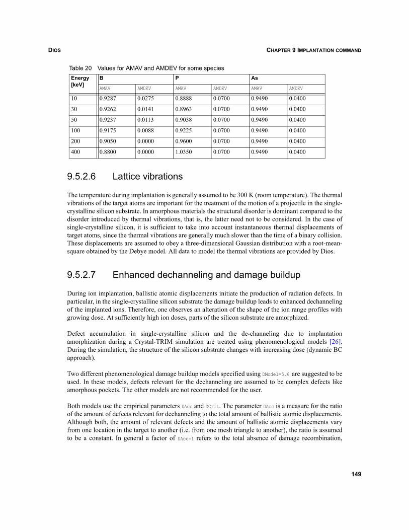
DIOS CHAPTER 9 IMPLANTATION COMMAND
9.5.2.6 Lattice vibrations
The temperature during implantation is generally assumed to be 300 K (room temperature). The thermalvibrations of the target atoms are important for the treatment of the motion of a projectile in the single-crystalline silicon substrate. In amorphous materials the structural disorder is dominant compared to thedisorder introduced by thermal vibrations, that is, the latter need not to be considered. In the case ofsingle-crystalline silicon, it is sufficient to take into account instantaneous thermal displacements oftarget atoms, since the thermal vibrations are generally much slower than the time of a binary collision.These displacements are assumed to obey a three-dimensional Gaussian distribution with a root-mean-square obtained by the Debye model. All data to model the thermal vibrations are provided by Dios.
9.5.2.7 Enhanced dechanneling and damage buildup
During ion implantation, ballistic atomic displacements initiate the production of radiation defects. Inparticular, in the single-crystalline silicon substrate the damage buildup leads to enhanced dechannelingof the implanted ions. Therefore, one observes an alteration of the shape of the ion range profiles withgrowing dose. At sufficiently high ion doses, parts of the silicon substrate are amorphized.
Defect accumulation in single-crystalline silicon and the de-channeling due to implantationamorphization during a Crystal-TRIM simulation are treated using phenomenological models [26].During the simulation, the structure of the silicon substrate changes with increasing dose (dynamic BCapproach).
Two different phenomenological damage buildup models specified using DModel=5,6 are suggested to beused. In these models, defects relevant for the dechanneling are assumed to be complex defects likeamorphous pockets. The other models are not recommended for the user.
Both models use the empirical parameters DAcc and DCrit. The parameter DAcc is a measure for the ratioof the amount of defects relevant for dechanneling to the total amount of ballistic atomic displacements.Although both, the amount of relevant defects and the amount of ballistic atomic displacements varyfrom one location in the target to another (i.e. from one mesh triangle to another), the ratio is assumedto be a constant. In general a factor of DAcc=1 refers to the total absence of damage recombination,
Table 20 Values for AMAV and AMDEV for some speciesEnergy [keV]
B P As
AMAV AMDEV AMAV AMDEV AMAV AMDEV
10 0.9287 0.0275 0.8888 0.0700 0.9490 0.0400
30 0.9262 0.0141 0.8963 0.0700 0.9490 0.0400
50 0.9237 0.0113 0.9038 0.0700 0.9490 0.0400
100 0.9175 0.0088 0.9225 0.0700 0.9490 0.0400
200 0.9050 0.0000 0.9600 0.0700 0.9490 0.0400
400 0.8800 0.0000 1.0350 0.0700 0.9490 0.0400
149
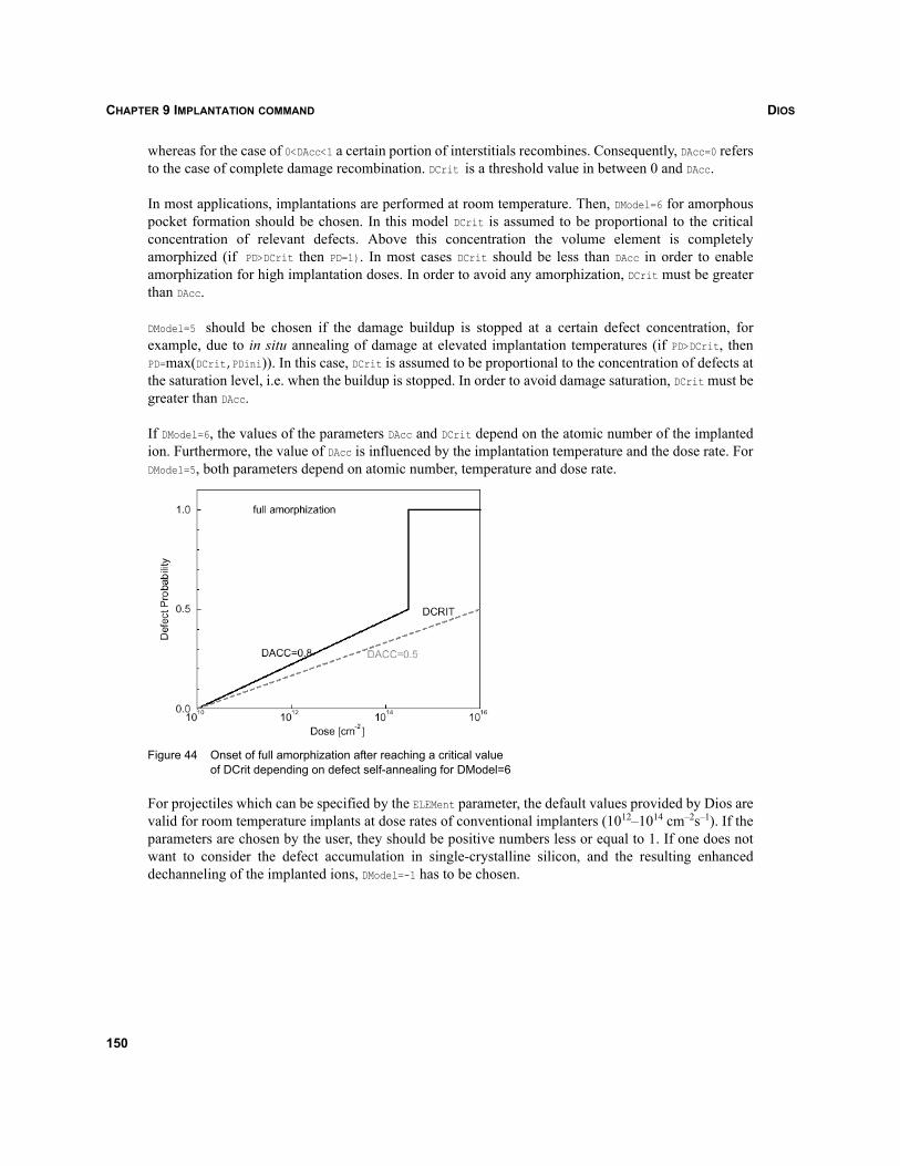
DIOSCHAPTER 9 IMPLANTATION COMMAND
whereas for the case of 0<DAcc<1 a certain portion of interstitials recombines. Consequently, DAcc=0 refersto the case of complete damage recombination. DCrit is a threshold value in between 0 and DAcc.
In most applications, implantations are performed at room temperature. Then, DModel=6 for amorphouspocket formation should be chosen. In this model DCrit is assumed to be proportional to the criticalconcentration of relevant defects. Above this concentration the volume element is completelyamorphized (if PD>DCrit then PD=1). In most cases DCrit should be less than DAcc in order to enableamorphization for high implantation doses. In order to avoid any amorphization, DCrit must be greaterthan DAcc.
DModel=5 should be chosen if the damage buildup is stopped at a certain defect concentration, forexample, due to in situ annealing of damage at elevated implantation temperatures (if PD>DCrit, thenPD=max(DCrit,PDini)). In this case, DCrit is assumed to be proportional to the concentration of defects atthe saturation level, i.e. when the buildup is stopped. In order to avoid damage saturation, DCrit must begreater than DAcc.
If DModel=6, the values of the parameters DAcc and DCrit depend on the atomic number of the implantedion. Furthermore, the value of DAcc is influenced by the implantation temperature and the dose rate. ForDModel=5, both parameters depend on atomic number, temperature and dose rate.
Figure 44 Onset of full amorphization after reaching a critical value of DCrit depending on defect self-annealing for DModel=6
For projectiles which can be specified by the ELEMent parameter, the default values provided by Dios arevalid for room temperature implants at dose rates of conventional implanters (1012–1014 cm–2s–1). If theparameters are chosen by the user, they should be positive numbers less or equal to 1. If one does notwant to consider the defect accumulation in single-crystalline silicon, and the resulting enhanceddechanneling of the implanted ions, DModel=-1 has to be chosen.
150
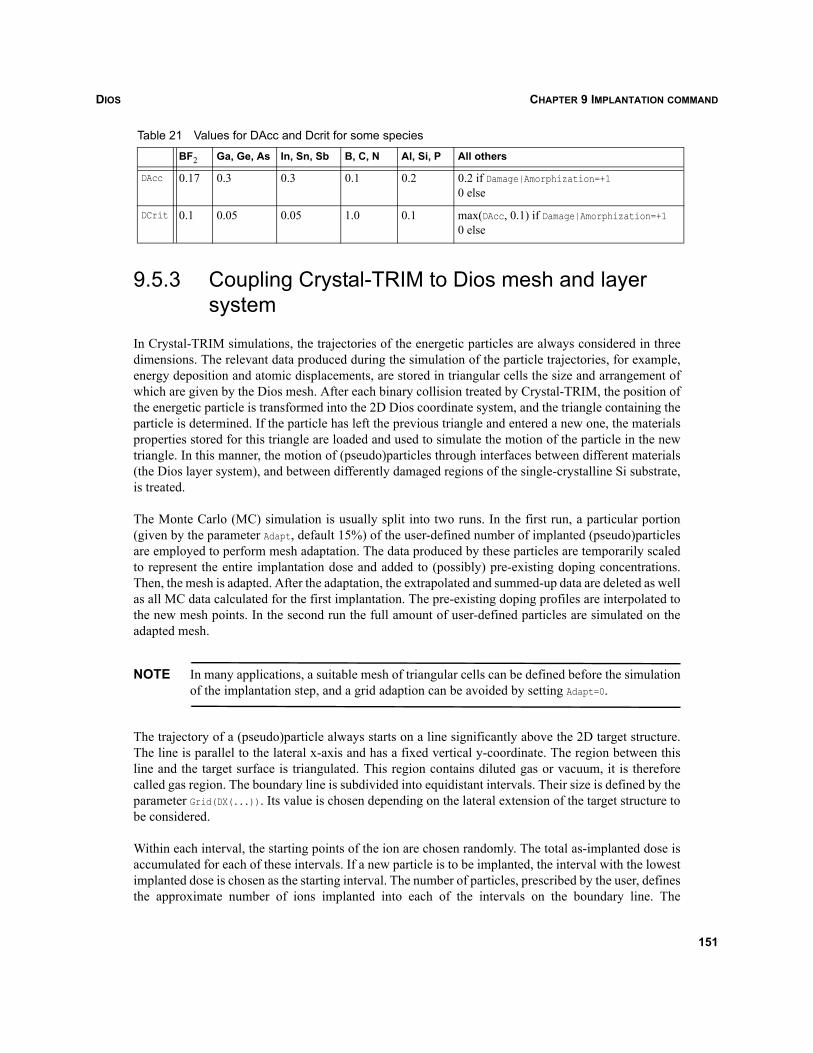
DIOS CHAPTER 9 IMPLANTATION COMMAND
9.5.3 Coupling Crystal-TRIM to Dios mesh and layer system
In Crystal-TRIM simulations, the trajectories of the energetic particles are always considered in threedimensions. The relevant data produced during the simulation of the particle trajectories, for example,energy deposition and atomic displacements, are stored in triangular cells the size and arrangement ofwhich are given by the Dios mesh. After each binary collision treated by Crystal-TRIM, the position ofthe energetic particle is transformed into the 2D Dios coordinate system, and the triangle containing theparticle is determined. If the particle has left the previous triangle and entered a new one, the materialsproperties stored for this triangle are loaded and used to simulate the motion of the particle in the newtriangle. In this manner, the motion of (pseudo)particles through interfaces between different materials(the Dios layer system), and between differently damaged regions of the single-crystalline Si substrate,is treated.
The Monte Carlo (MC) simulation is usually split into two runs. In the first run, a particular portion(given by the parameter Adapt, default 15%) of the user-defined number of implanted (pseudo)particlesare employed to perform mesh adaptation. The data produced by these particles are temporarily scaledto represent the entire implantation dose and added to (possibly) pre-existing doping concentrations.Then, the mesh is adapted. After the adaptation, the extrapolated and summed-up data are deleted as wellas all MC data calculated for the first implantation. The pre-existing doping profiles are interpolated tothe new mesh points. In the second run the full amount of user-defined particles are simulated on theadapted mesh.
NOTE In many applications, a suitable mesh of triangular cells can be defined before the simulationof the implantation step, and a grid adaption can be avoided by setting Adapt=0.
The trajectory of a (pseudo)particle always starts on a line significantly above the 2D target structure.The line is parallel to the lateral x-axis and has a fixed vertical y-coordinate. The region between thisline and the target surface is triangulated. This region contains diluted gas or vacuum, it is thereforecalled gas region. The boundary line is subdivided into equidistant intervals. Their size is defined by theparameter Grid(DX(...)). Its value is chosen depending on the lateral extension of the target structure tobe considered.
Within each interval, the starting points of the ion are chosen randomly. The total as-implanted dose isaccumulated for each of these intervals. If a new particle is to be implanted, the interval with the lowestimplanted dose is chosen as the starting interval. The number of particles, prescribed by the user, definesthe approximate number of ions implanted into each of the intervals on the boundary line. The
Table 21 Values for DAcc and Dcrit for some species
BF2 Ga, Ge, As In, Sn, Sb B, C, N Al, Si, P All others
DAcc 0.17 0.3 0.3 0.1 0.2 0.2 if Damage|Amorphization=+1 0 else
DCrit 0.1 0.05 0.05 1.0 0.1 max(DAcc, 0.1) if Damage|Amorphization=+10 else
151
DIOSCHAPTER 9 IMPLANTATION COMMAND
coordinates of the incident ions with respect to the second horizontal dimension (z), perpendicular to the2D target structure, are also selected randomly within a distance characteristic for the lattice structure ofthe single-crystalline Si substrate. In the special case where the x-axis and z-axis are identical to the<100> and <001> crystal directions, respectively, this distance is equal to the lattice constant.
A (pseudo)particle starting at the boundary line moves on a straight line through the gas region and hitsthe target surface. Only the motion within the target material is simulated by Crystal-TRIM. If particlesleave the target, they continue their motion on a straight line through the gas region until they enter thetarget again, or they pass the boundary of the 2D target structure either through the gas region or throughthe material on the left and right side of the 2D target structure.
Since no particles can enter the structure on the left and right side, the profiles of the implanted dopantsdecay at both sides. In order to avoid this artificial effect, before the MC simulation, the 2D structureand the simulation grid are expanded to the left and right side. After the simulation, the grid is reducedautomatically to the initial size. The expansion can be defined by the user, applying the parametersLeftOffset and RightOffset. The default is set to 7.5 times the lateral straggling of a point responseprofile.
NOTE If the target structure exhibits a 1D symmetry (or if a 1D grid is used), the structure is notexpanded. Periodic or reflecting boundary conditions are used instead. Users can enforcethese boundary conditions in 2D using BoundaryCondition=Periodic orBoundaryCondition=Reflection (however, BoundaryCondition=No is default for 2D structures).
9.5.4 Statistical enhancement techniques
9.5.4.1 Trajectory splitting
Usually, the dopant concentration has to be predicted precisely for several orders of magnitude. Theregions of low concentration are mainly due to deep channeling tails and lateral channeling brancheswhich are caused by a small number of incident ions with particularly long trajectories.
To obtain a smooth distribution of implanted dopants in such regions, the number of (pseudo)particletrajectories that had to be simulated was tremendously high, and the computing time was very long. Theuse of a splitting algorithm increases the computational efficiency and decreases the statistical noise byseveral orders of magnitude.
The basic idea is to artificially increase the number of so-called rare-event trajectories calculated inregions with low trajectory density (importance sampling). If one mother projectile reaches a triangle ofsmall trajectory density, a splitting point is set, that is, that it is replaced by two daughter projectiles eachhaving half the statistical weight of the mother projectile. The current status of the mother projectile, forexample, position, energy, direction of motion as well as the positions of neighboring target atoms, inparticular those of the last collision partners, are stored. The trajectory of the first daughter projectile isfollowed.
152
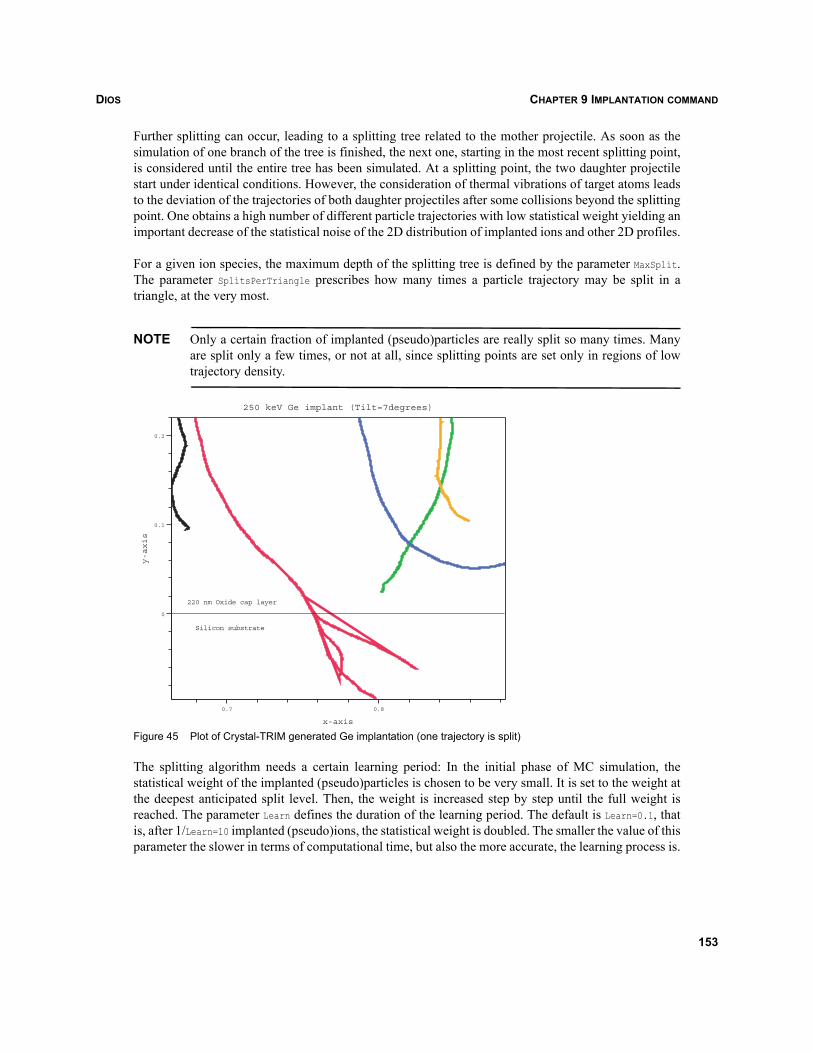
DIOS CHAPTER 9 IMPLANTATION COMMAND
Further splitting can occur, leading to a splitting tree related to the mother projectile. As soon as thesimulation of one branch of the tree is finished, the next one, starting in the most recent splitting point,is considered until the entire tree has been simulated. At a splitting point, the two daughter projectilestart under identical conditions. However, the consideration of thermal vibrations of target atoms leadsto the deviation of the trajectories of both daughter projectiles after some collisions beyond the splittingpoint. One obtains a high number of different particle trajectories with low statistical weight yielding animportant decrease of the statistical noise of the 2D distribution of implanted ions and other 2D profiles.
For a given ion species, the maximum depth of the splitting tree is defined by the parameter MaxSplit.The parameter SplitsPerTriangle prescribes how many times a particle trajectory may be split in atriangle, at the very most.
NOTE Only a certain fraction of implanted (pseudo)particles are really split so many times. Manyare split only a few times, or not at all, since splitting points are set only in regions of lowtrajectory density.
Figure 45 Plot of Crystal-TRIM generated Ge implantation (one trajectory is split)
The splitting algorithm needs a certain learning period: In the initial phase of MC simulation, thestatistical weight of the implanted (pseudo)particles is chosen to be very small. It is set to the weight atthe deepest anticipated split level. Then, the weight is increased step by step until the full weight isreached. The parameter Learn defines the duration of the learning period. The default is Learn=0.1, thatis, after 1/Learn=10 implanted (pseudo)ions, the statistical weight is doubled. The smaller the value of thisparameter the slower in terms of computational time, but also the more accurate, the learning process is.
220 nm Oxide cap layer
Silicon substrate
250 keV Ge implant (Tilt=7degrees)
x-axis
0.7 0.8
y-axis
0
0.1
0.2
153
DIOSCHAPTER 9 IMPLANTATION COMMAND
NOTE If you do not want to use the splitting procedure, for example, if you are not interested inchanneling tails, it can be switched off by setting MaxSplit=0.
9.5.4.2 Lateral replication
The lateral extension of the 2D target structures is usually large compared to the length of the trajectoryof an implanted ion. Therefore, a lot of (pseudo)particles have to be started at different points on theboundary line parallel to the x-axis. This may lead to a very long computing time. However, in mostapplications different lateral regions can have similar properties, for example, nearly the same depthstructure and lateral environment, showing nearly 1D symmetry. Therefore, the trajectories of(pseudo)particles started at a given x-coordinate can be copied to other starting points within theseregions [23]. This procedure is called lateral replication, and it increases the number of ion trajectoriesin these regions without additional computational effort.
At the beginning of MC simulation all intervals at the boundary line parallel to the x-axis are labeledwith the same index assigning them to the same equivalence class. During the simulation of an iontrajectory, for each triangle passed, the material composition as well as the increment of dopant anddamage concentration in this triangle are stored. The material arrangement and the damage state in theinterval are compared to the other intervals. In cases where no mismatch is found, the 2D distributionsare copied to all these intervals then belonging to the same equivalence class. Otherwise thecorresponding starting interval on the boundary line is assigned to a new equivalence class.
Since in different lateral regions the material arrangement and the damage state are seldom exactly thesame, a small tolerance for a mismatch is allowed. The tolerance region can be specified by theparameter EquivLength (default 3 nm). Within the range given by this parameter the material arrangementand the damage state are not distinguished. If a particle re-enters the gas region, the interval on theboundary line where the particle was started, is put into a separate equivalence class and no transfer oftrajectories of this class are performed anymore. In this manner mask edge and trench implantations canbe treated without essential approximations.
The subdivision into very different equivalence classes takes place at the very beginning of the MCsimulation. Therefore, the error which occurs by copying 2D distributions to lateral intervals which arefound to be not equivalent in further steps of the simulation is relatively small. The equivalence classsubdivision is terminated after EquivStop (default 15%) of the as-implanted dose is processed. Trajectorieswhich are started later and which do not fit to an existing equivalence class are not copied and no newequivalence class is built.
NOTE Due to the complicated nature of the replication procedure the user can hardly estimate thenumber of ion trajectories which are really simulated, that is, the difference between the totalnumber of incident (pseudo)particles (given by the number of lateral intervals of widths DXmultiplied with Particles) and the number of replicated trajectories (this number is providedin the Dios standard output during the simulation run).
154
DIOS CHAPTER 9 IMPLANTATION COMMAND
If the user specifies Intervals=1, the boundary line is not subdivided into intervals (see above). Then nolateral transfer is made and only original particle trajectories are computed. This is usually much moretime consuming but can be used to check the influence of the lateral replication on the simulation results.Also, no lateral trajectory transfer is done at all, if a 1D structure with a 1D grid is considered.
9.5.4.3 Statistical reliability checking
In order to check the statistical reliability of the results of MC simulations, in particular after performingtrajectory splitting, the parameter Significance was introduced. The datasets generated if Significance isnot equal to No are only temporarily defined. They can be displayed by the Dios graphics immediatelyafter the MC simulations.
If Significance=OriginalParticles, in each triangle the contributions to the dopant and damageconcentration are classified with respect to the original (pseudo-)particles started at the boundary line ontop of the gas region. This includes replicated particles as well. For each triangle the number ofcontributing original particles is counted. The 2D distribution of these numbers is given in the data setNumberOfIons_*, for example, NumberOfIons_Arsenic for arsenic implants. Therefore, the data setNumberOfIons_* can be used to analyze the statistical reliability of low-concentration parts of the 2Ddopant distributions. As described above, the smoothness of these parts is increased artificially due tothe trajectory splitting. However, if only a small number of original particles contributed to a certainlow-concentration part of the 2D distribution, the simulation results are not statistically reliable. Ingeneral, data in triangles resulting from less than 10-15 original particles may not be regarded asstatistically reliable.
Alternatively, the statistical reliability of the simulation results can be assessed usingSignificance=MaxShare. Here, in each triangle the number of binary collisions is counted for every originalparticle. After the MC simulation is finished, the number of the particle with the maximum number ofcollisions is stored in the data set MaxIon_*. The ratio of the number of collisions of this particle and thetotal number of collisions in the triangle is stored in the dataset MaxDeltaPlc_*. If one particle contributesmore than 10–20% of the binary collisions in a triangle, the simulation results in this triangle cannot beconsidered as statistically reliable.
9.5.4.4 XGRAPH representation of trajectories
The trajectories of the implanted (pseudo)particles can be stored into a series of files in XGRAPHformat. In the parameter record Trajectories different parameters (File, Particles, First, Last, List=(...),Shift, MinLength) can be specified. The file name can be prescribed, a counter and the file extension .plxare appended internally. The parameter Particles=No|All|Gas|Leaving|Visitor can be specified to selectthe trajectories, for example, to save only particle trajectories, if they enter the gas, leave the grid at thesymmetry lines, or if they are visiting a certain triangle. A range or a list of particle numbers can bespecified. If Shift=on, all trajectories are moved to start in the origin. Additionally, the parameter recordTriangles(First, Last, List=(...)) can be used, to select the triangles for Particles=Visitor and to printinto the protocol which particles come to rest in the specified triangles.
155
DIOSCHAPTER 9 IMPLANTATION COMMAND
9.6 Implantation damageFor the simulation of transient-enhanced diffusion (TED) phenomena, modeling of the implantationdamage and amorphization is very important. Implantation damage refers to modifications of the defectdensities, that is, the interstitial (ITot), vacancy (VTot) and interstitial trap (ITrapTotal) datasets.
The damage model is selected using:
Implantation:(Damage=No|+1|Hobler|MCDamage))
The various defect profiles need not be defined when using the conventional or equilibrium diffusionmodels. For these models, only during oxidation a meaningful interstitial profile is computed. It willoverride any profile previously defined. For the point defect based diffusion models the interstitial,vacancy, and trap profiles are introduced once when necessary and then kept at all times, similar to thedoping profiles.
A dataset Amorphization is introduced during the ion implantation simulation and removed after the firstaccepted time step of a subsequent anneal process. During subsequent implantation steps theamorphization dataset keeps the accumulated implantation damage (damage history). The data valuescan be considered as the concentration of Frenkel (I+V) pairs. The amorphization model is selectedsimilar to the damage model, that is:
Implantation:(Amorphization=No|+1|Hobler|MCDamage)
The amorphization dataset is used to determine wether a particular region is crystalline or amorphous.If the resulting value of Amorphization at a particular mesh point exceeds the Threshold density of
, the material is assumed to be amorphized. The dataset Amorphization is cut at the Thresholdvalue.
For Damage|Amorphization=No, no defect densities or amorphization densities are computed and added tothe existing datasets.
Further control over the handling of total defect concentrations in amorphized or nonamorphized regionsis provided with the data records ILocation, VLocation and ITrapLocation:
Implantation(ILocation(Amorphized=Add|Keep|Delete|Replace))
The Delete option is default for amorphized regions which means that the interstitial density is set to itsminimum allowed value. In non amorphized regions the default is Add which leads to interstitialaccumulation. These records are only available using analytic distribution functions.
NOTE ELEMent=I can be specified to simulate a silicon preamorphization. One can also specifyElement=V|Amorphization|ITrapTotal|ITrapEmpty or any other Dios variable name (seeAppendix A on page 315) in an Implantation command. In this case, the moments are takenfrom arsenic. Damage=No and Amorphization=No should be used for such implantation steps. Theas-implanted profile is added to the specified dataset. This can be used similar to the Loadcommand, with the main difference, that in the Implantation command the layer system istaken into account.
1.15 1022×
156
DIOS CHAPTER 9 IMPLANTATION COMMAND
9.6.1 Analytic damage models
Defect profiles and the amorphization on the basis of analytic damage models can be generated usingeither the +1 or the more sophisticated Hobler model [22].
NOTE Damage|Amorphization=MCDamage is not available in analytic implantation. In MC implantationcalculations, (Implantation(FUNCtion=CrystalTrim)) Damage|Amorphization=Hobler switchesinternally to Damage|Amorphization=MCDamage.
For Damage=+1, the as-implanted dopant profile, and for Damage=Hobler, the Hobler damage is used andmultiplied with IFactor and VFactor in order to generate the respective defect density. This is then addedto the already existing total interstitial or total vacancy densities (remaining from preceding diffusionsteps). By default, IFactor=undefined and VFactor=undefined. The internal default values depend on theuser-defined values of IFactor and CritDose. If CritDose is undefined, the given value of IFactor will beused. Otherwise, IFactor is taken from:
(32)
The internal default values are IFactor=2 and CritDose=1.5e14/cm2 for arsenic and IFactor=2 andCritDose=1.125e14/cm2 for boron. This is motivated by the results of special marker experiments. For theother dopants, the internal default is IFactor=1 and CritDose=undefined.
The assumption of the so-called +1 model is motivated by a simple lattice site balance: For each dopantatom, which is assumed after implantation on a lattice site, one (free) interstitial is produced, or to bemore general one should always assume IFactor=VFactor+1. If only the value for IFactor is specified orif the internal default values are used and if the value of IFactor>1, this relation will always be assumedin Dios. If the given or computed value of IFactor<1, internally, VFactor=0 is used by default. Sincenothing is known about initial point defect profiles, IFactor and VFactor are the preferred fit parametersfor TED simulation. ITrapFactor is used to generate the ITrapTotal profile.
In Monte Carlo calculations with Crystal-TRIM, it is also possible to use the analytic Damage=+1 damagemodel. The total interstitial and vacancy density is derived from the ION1...3 dataset that stores the as-implanted dopant profile in a similar manner then in analytic implantation, that is:
In a full-cascade run (Cascades=On) of Crystal-TRIM with Damage=+1 the following relation is used:
IFactor IFactor min 1 CritDoseDose
-------------------------------,⎝ ⎠⎛ ⎞⋅=
ITotal ION1 IFactor⋅←
VTotal ION1 VFactor⋅←
VTotal ION1 VFactor max MCVFactor IVAC MCIFactor RCL1 0,⋅–⋅( )+⋅←
ITotal ION1 IFactor max MCIFactor RCL1 MCVFactor IVAC 0,⋅–⋅( )+⋅←
157
DIOSCHAPTER 9 IMPLANTATION COMMAND
NOTE The above functions for Cascades=On do not give an exact +1 model behavior since thedifference between the ballistic interstitial and vacancy profiles is taken into account.
For Amorphization=+1, the as-implanted dopant profile, and for Amorphization=Hobler the Hobler damageis used for the detection of amorphized regions. The selected profile is multiplied with AFactor (default1) and the result is added to the dataset Amorphization. This summation is assumed to account for theaccumulation of dose during split implantations. In Monte Carlo calculations AFactor is used to calculatethe Dios Amorphization dataset from the Crystal-TRIM datasets ION1...3.
9.6.2 Monte Carlo damage
In Monte Carlo simulations using Crystal-TRIM, the implantation damage can be calculated directlyfrom the ballistic interstitial and vacancy datasets using Damage=MCDamage. The Dios parameters MCIFactorand MCVFactor are used to generate the defect densities from the Crystal-TRIM datasets RCL1...3(interstitials) and IVAC (vacancies) if Cascades=On:
The default value for MCIFactor and MCVFactor is 1. If Cascades=Off, only the ballistic vacancy density IVACis calculated by Crystal-TRIM and used to initialize both ITotal and VTotal:
The Dios Amorphization dataset is initialized after an implantation step from the Crystal-TRIM dataset PD(damage probability) and cut off at the Threshold value, that is:
where Threshold is set according to Implantation(Threshold=).
Consequently, for Damage=MCDamage, Threshold has no effect on the amorphization layer thickness.Adjustments to DACC and DCRIT can be used to change the thickness of the amorphized layer (seeSection 9.5.2.7 on page 149 for more information about DACC and DCRIT).
The amorphization history is always stored in the Amorphization dataset even if a diffusion step has beenperformed between implants. Before an implantation step, PD is initialized using the Amorphizationdataset. If there was a preceding diffusion step, the values in the Amorphization dataset will be set to zeroautomatically.
VTotal IVAC MCVFactor⋅←
ITotal RCL1 MCIFactor⋅←
VTotal IVAC VFactor⋅←
ITotal IVAC IFactor⋅←
Amorphization PD Threshold⋅←
158
DIOS CHAPTER 9 IMPLANTATION COMMAND
9.7 Transition to diffusionThe recrystallization of amorphized regions is not modeled in Dios. It is assumed, that the regrowth isfast and finished when the starting temperature of the anneal step, following the implantation, is reached(that is, no diffusion, just the recrystallization front was moving through the amorphized regions, leavingcrystalline material behind with high activation level and equilibrium point defect concentrations). Thus,the initial profiles of ITotal and VTotal in the amorphized regions are set to their equilibrium values atthe start temperature of the anneal and the amorphized region flag is removed.
The initial point defect profiles ITotal and VTotal outside of the amorphized layer also reflect the residualdamage at the start temperature (after a fast local initial recombination with no diffusion). Thus theirpeak value may not reach the amorphization level. The concentrations of ITotal and VTotal are notcompared to Threshold and thus have no influence on the detection of amorphized layers.
NOTE For the dopant species, an initial full activation is assumed in the amorphized layers bydefault. One may use the parameters Diffusion(ACInit) and Diffusion(Si(Aj(ACInit))) tocontrol the initial values for the activation level (of dopant Aj).
9.8 Monte Carlo implantation in 3DThe Monte Carlo simulation for 3D structures is performed by a system call of the stand-alone simulatorimplant3d. The implanted tool converts the appropriate DF–ISE boundary files into files, suitable for theMonte Carlo simulator. Then, it calls the Monte Carlo simulation and converts the results back intoDF–ISE files. These files are used in DIP, when building the 3D grid with Mesh. The process simulatorDios is used only to translate the parameters from the input file into the appropriate command files forimplant3d and Mesh, and to provide the geometry input files in DF–ISE format.
The stand-alone Monte Carlo simulator, which was developed at TU Vienna and is integrated in theimplant3d tool was named MCIMPL [6][29]. A brief description is in Appendix V on page 605.
159

DIOSCHAPTER 9 IMPLANTATION COMMAND
160
DIOS CHAPTER 10 DIFFUSION COMMAND
Dios
CHAPTER 10 Diffusion command
10.1 OverviewDuring all high temperature processes, dopant redistribution is caused by dopant and point defectdiffusion, by chemical reactions at the interfaces and inside the layers, and by convective dopanttransport due to internal electrical fields as well as material flow and moving material interfaces. In Dios,the Diffusion command is used to simulate all high temperature steps. The various process atmospheresare described by the parameter Atmosphere=O2 | HCl | H2O | H2O2 | H2N2 | N2 | Epitaxy | Prebake |Mixture. Additional parameters can be specified to describe the composition of the process gas in moredetail. Appendix I on page 375 lists the Diffusion command parameters.
For NewDiff=0 and the combination of NewDiff=1 and SiDiff=on, the diffusion equations are solved in thesilicon only. In these modes, all overlayers are used only as ‘decoration’ to select appropriate boundaryconditions and for the correct simulation of the ion implantation. For these modes, the segregation effectcan be simulated only during oxidation. For the combination NewDiff=1 SiDiff=off, diffusion is simulatedin all materials except gas. The segregation effect can be simulated for all diffusion steps but thesimulation may take a significantly longer time since all mesh points in the overlayers have to be takeninto account. In addition, the stiffness of the diffusion equations is significantly increased.
The diffusion model can be selected with a global model switch:
DIFFusion(ModDiff=Conventional | Equilibrium | LooselyCoupled | SemiCoupled | PairDiffusion)
The Conventional and Equilibrium diffusion models are very similar. Point defects are involved onlyduring the oxidation and only via empirical models of modified dopant diffusivities. The main differencebetween the two models is the numeric scheme and the implementation. For the Conventional model, ablock iteration similar to the Gummel scheme for device simulation is used. On top of this (only) forModDiff=Conventional a specific diffusion model can be selected for each of the materials and each of thedopants. Formally, all models can be applied in all layers, the default values just point to preferredmodels and parameters. Model parameters for boron, arsenic, and phosphorus have been adjusted in thedaily use of the simulator for process simulation, by comparing 1D cross sections with the result of 1Dsimulations with TESIM-4 and with SIMS data. The data for antimony, aluminum, gallium, indium,germanium, and nitrogen has not been tested greatly, and some of the specific parameters have beencollected from literature, but most of the unknown parameters have been copied from arsenic or boron.
The diffusivities for ModDif=Equilibrium model correspond to the SUPREM-III diffusivity for theConventional model. The Equilibrium model is implemented as the most simplified version within the‘point defect solver,’ that is, the simplest model of the series of diffusion models Equilibrium,LooselyCoupled, SemiCoupled, and PairDiffusion. For each of these models, the diffusion mechanism insilicon can only be chosen once for all dopants. Only the coefficients and immobility (clustering)reactions can be defined per dopant. For all of these models and all dopants, the same diffusion modelis always applied in polycrystalline material and the same model is always applied in amorphousmaterials. Transient diffusion effects can be simulated with any of LooselyCoupled, SemiCoupled, or
161
DIOSCHAPTER 10 DIFFUSION COMMAND
PairDiffusion models. A dopant pile-up towards the gate oxide, which is often used to explain the reverseshort-channel effect, can be simulated only with the PairDiffusion model. The ModDiff selection for alldopants can be changed during a simulation. Unexpected side effects from remaining or missing, forexample, interstitial concentrations (OED/damage), can be resolved by using theLoad(Type=Remove, Species(...)) command.
The diffusion parameters are defined for all dopants and all materials separately. Sometimes, parametershave been defined only if useful default values are known. This may restrict the possibility to overridemodels and parameters, and ‘rename’ materials or dopant species for user-defined material–dopantcombinations.
10.2 Coupled diffusion of dopants and point defects: Point defect solver
For all but the Conventional diffusion model, the same numeric scheme is used. This scheme is referredto in this manual as the ‘point defect solver.’ The level of sophistication of the interaction of silicon pointdefects and dopant species in this scheme is selected with the ModDiff switch. For all models of the pointdefect solver, the balance equations are always written for the total concentrations of point defects and/or dopant species. The total concentrations are the (global) solution variables, for which the incrementsare calculated in the (global) Newton iteration. Besides these global equations, in every mesh point, alocal system of algebraic and ordinary differential equations (ordinary differential equations with respectto time) are solved to derive the substitutional dopant concentrations, the concentrations of neutralunpaired point defects, the concentrations of clusters, electrons, and so on, and all the derivatives ofthese local variables with respect to the global solution variables.
The final selection and validity check and perhaps modification of the initial profiles is performed at thebeginning of the anneal step, since only at that time will the start temperature of the ramp be suppliedby the user. This can be controlled with a few global parameters in the Diffusion command. The finallychosen initial values cannot be checked in the Dios graphics. The only possibility is to define a verysmall duration of the anneal or to redraw after a very small initial time step.
The diffusion model used for ModDiff=PairDiffusion has been explained in the literature [24]. It was alsothe basic model used in [25]. From this model, all other diffusion models are derived as simplificationswith the help of additional assumptions on the concentrations, diffusivities, or reaction terms. The modelassumptions are explained in the subsequent sections starting with the computation of the diffusivitiesin the PairDiffusion model (see Section 10.2.8 on page 176). In Section 10.2.9 on page 181, thesimplifications for the SemiCoupled model are introduced followed in Section 10.2.10 on page 183 by theassumptions for the LooselyCoupled model. Section 10.2.11 on page 186 describes the assumptions forthe Equilibrium model.
For the PairDiffusion model, point defect–dopant pairs and unpaired point defects are the assumedmobile species. All electronic and pairing reactions are assumed to be in equilibrium. Theelectrochemical potential of the pairs is the driving force for the pair flux, that is, the gradient of theproduct of the substitutional dopant concentration, the electron density (field term), and theconcentration of neutral unpaired point defects drive the dopant diffusion. The pair fluxes contribute toboth the diffusion of dopants and point defects. At interfaces, a normal flux of interstitials may be
162
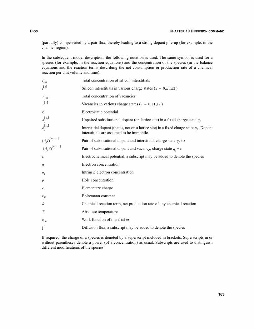
DIOS CHAPTER 10 DIFFUSION COMMAND
(partially) compensated by a pair flux, thereby leading to a strong dopant pile-up (for example, in thechannel region).
In the subsequent model description, the following notation is used. The same symbol is used for aspecies (for example, in the reaction equations) and the concentration of the species (in the balanceequations and the reaction terms describing the net consumption or production rate of a chemicalreaction per unit volume and time):
Total concentration of silicon interstitials
Silicon interstitials in various charge states ( )
Total concentration of vacancies
Vacancies in various charge states ( )
Electrostatic potential
Unpaired substitutional dopant (on lattice site) in a fixed charge state
Interstitial dopant (that is, not on a lattice site) in a fixed charge state . Dopantinterstitials are assumed to be immobile.
Pair of substitutional dopant and interstitial, charge state
Pair of substitutional dopant and vacancy, charge state
Electrochemical potential, a subscript may be added to denote the species
Electron concentration
Intrinsic electron concentration
Hole concentration
Elementary charge
Boltzmann constant
Chemical reaction term, net production rate of any chemical reaction
Absolute temperature
Work function of material m
Diffusion flux, a subscript may be added to denote the species
If required, the charge of a species is denoted by a superscript included in brackets. Superscripts in orwithout parentheses denote a power (of a concentration) as usual. Subscripts are used to distinguishdifferent modifications of the species.
Itot
I z[ ] z 0 1 2±,±,=
Vtot
V z[ ] z 0 1 2±,±,=
ϕ
Ajqj[ ]
qj
Bjpj[ ]
pj
AjI( )qj z+[ ]
qj z+
AjV( )qj z+[ ]
qj z+
ς
n
ni
p
e
kB
R
T
ϕm
j
163
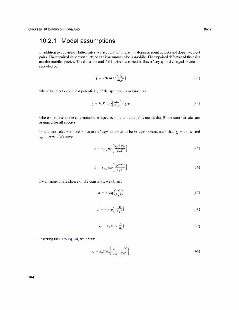
DIOSCHAPTER 10 DIFFUSION COMMAND
10.2.1 Model assumptions
In addition to dopants on lattice sites, we account for interstitial dopants, point defects and dopant–defectpairs. The unpaired dopant on a lattice site is assumed to be immobile. The unpaired defects and the pairsare the mobile species. The diffusion and field-driven convection flux of any q-fold charged species ismodeled by:
(33)
where the electrochemical potential of the species c is assumed as:
(34)
where c represents the concentration of species c. In particular, this means that Boltzmann statistics areassumed for all species.
In addition, electrons and holes are always assumed to be in equilibrium, such that and. We have:
(35)
(36)
By an appropriate choice of the constants, we obtain:
(37)
(38)
(39)
Inserting this into Eq. 34, we obtain:
(40)
j Dcgradς
kBT---------
⎝ ⎠⎛ ⎞–=
ς
ς kBT c
cref--------
⎝ ⎠⎜ ⎟⎛ ⎞
qeϕ+log=
ςn const=ςp const=
n nrefςn eϕ+
kBT------------------
⎝ ⎠⎜ ⎟⎛ ⎞
exp=
p prefςp eϕ–
kBT-----------------
⎝ ⎠⎜ ⎟⎛ ⎞
exp=
n nieϕkBT---------
⎝ ⎠⎛ ⎞exp=
p nieϕkBT---------–⎝ ⎠
⎛ ⎞exp=
eϕ kBTnni----
⎝ ⎠⎛ ⎞log=
ς kBTc
cref--------
nni----
⎝ ⎠⎛ ⎞ q
⋅⎝ ⎠⎜ ⎟⎛ ⎞
log=
164
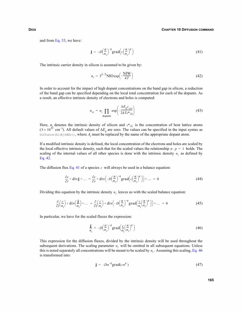
DIOS CHAPTER 10 DIFFUSION COMMAND
and from Eq. 33, we have:
(41)
The intrinsic carrier density in silicon is assumed to be given by:
(42)
In order to account for the impact of high dopant concentrations on the band gap in silicon, a reductionof the band gap can be specified depending on the local total concentration for each of the dopants. Asa result, an effective intrinsic density of electrons and holes is computed:
(43)
Here, ni denotes the intrinsic density of silicon and is the concentration of host lattice atoms( cm–3). All default values of ΔEg are zero. The values can be specified in the input syntax asDiffusion(Si(Aj(DEG))), where Aj must be replaced by the name of the appropriate dopant atom.
If a modified intrinsic density is defined, the local concentration of the electrons and holes are scaled bythe local effective intrinsic density, such that for the scaled values the relationship holds. Thescaling of the internal values of all other species is done with the intrinsic density as defined byEq. 42.
The diffusion flux Eq. 41 of a species will always be used in a balance equation:
(44)
Dividing this equation by the intrinsic density leaves us with the scaled balance equation:
(45)
In particular, we have for the scaled fluxes the expression:
(46)
This expression for the diffusion fluxes, divided by the intrinsic density will be used throughout thesubsequent derivations. The scaling parameter will be omitted in all subsequent equations. Unlessthis is noted separately all concentrations will be meant to be scaled by . Assuming this scaling, Eq. 46is transformed into:
(47)
j Dnni----
⎝ ⎠⎛ ⎞ q–
grad cnni----
⎝ ⎠⎛ ⎞ q
⎝ ⎠⎛ ⎞–=
ni T3 2⁄ NIO NIWkT
-------------–⎝ ⎠⎛ ⎞exp=
nie ni
ΔEgctot
2kTc∗Si-------------------–
⎝ ⎠⎜ ⎟⎛ ⎞
expdopants∏=
c∗Si5 1022×
n p⋅ 1=ni
c
t∂∂c divj …+ + t∂
∂c div Dnni----
⎝ ⎠⎛ ⎞ q–
grad cnni----
⎝ ⎠⎛ ⎞ q
⎝ ⎠⎛ ⎞–⎝ ⎠
⎛ ⎞ …+ + 0= =
ni
t∂∂ c
ni----⎝ ⎠
⎛ ⎞ div jni----⎝ ⎠
⎛ ⎞ …+ +t∂
∂ cni----⎝ ⎠
⎛ ⎞ div Dnni----
⎝ ⎠⎛ ⎞ q–
grad cni----
nni----
⎝ ⎠⎛ ⎞ q
⎝ ⎠⎛ ⎞–⎝ ⎠
⎛ ⎞ …+ + 0= =
jni---- D
nni----
⎝ ⎠⎛ ⎞ q–
grad cni----
nni----
⎝ ⎠⎛ ⎞ q
⎝ ⎠⎛ ⎞–=
nini
j Dn q– grad cnq( )–=
165
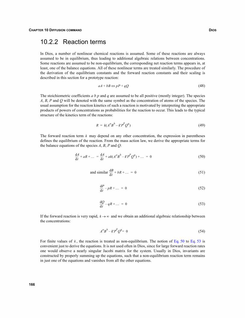
DIOSCHAPTER 10 DIFFUSION COMMAND
10.2.2 Reaction terms
In Dios, a number of nonlinear chemical reactions is assumed. Some of these reactions are alwaysassumed to be in equilibrium, thus leading to additional algebraic relations between concentrations.Some reactions are assumed to be non-equilibrium, the corresponding net reaction terms appears in, atleast, one of the balance equations. All of these nonlinear terms are treated similarly. The procedure ofthe derivation of the equilibrium constants and the forward reaction constants and their scaling isdescribed in this section for a prototype reaction:
(48)
The stoichiometric coefficients a b p and q are assumed to be all positive (mostly integer). The speciesA, B, P and Q will be denoted with the same symbol as the concentration of atoms of the species. Theusual assumption for the reaction kinetics of such a reaction is motivated by interpreting the appropriateproducts of powers of concentrations as probabilities for the reaction to occur. This leads to the typicalstructure of the kinetics term of the reactions:
(49)
The forward reaction term may depend on any other concentration, the expression in parenthesesdefines the equilibrium of the reaction. From the mass action law, we derive the appropriate terms forthe balance equations of the species A, B, P and Q:
(50)
and similar (51)
(52)
(53)
If the forward reaction is very rapid, and we obtain an additional algebraic relationship betweenthe concentrations:
(54)
For finite values of , the reaction is treated as non-equilibrium. The notion of Eq. 50 to Eq. 53 isconvenient just to derive the equations. It is not used often in Dios, since for large forward reaction ratesone would observe a nearly singular Jacobi matrix for the system. Usually in Dios, invariants areconstructed by properly summing up the equations, such that a non-equilibrium reaction term remainsin just one of the equations and vanishes from all the other equations.
aA bB pP qQ+⇔+
R k AaBb k'P–pQq( )=
k
tddA aR …+ +
tddA ak AaBb k'P–
pQq( ) …+ + 0= =
tddB bR …+ + 0=
tddP pR– …+ 0=
tddQ qR– …+ 0=
k ∞→
AaBb k'P–pQq 0=
k
166
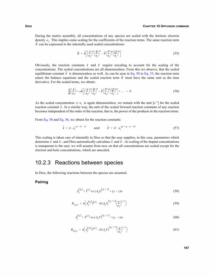
DIOS CHAPTER 10 DIFFUSION COMMAND
During the matrix assembly, all concentrations of any species are scaled with the intrinsic electrondensity . This implies some scaling for the coefficients of the reaction terms. The same reaction term
can be expressed in the internally used scaled concentrations:
(55)
Obviously, the reaction constants and require rescaling to account for the scaling of theconcentrations. The scaled concentrations are all dimensionless. From this we observe, that the scaledequilibrium constant is dimensionless as well. As can be seen in Eq. 50 to Eq. 53, the reaction termenters the balance equations and the scaled reaction term must have the same unit as the timederivative. For the scaled terms, we obtain:
(56)
As the scaled concentration is again dimensionless, we remain with the unit [s–1] for the scaledreaction constant . In a similar way, the unit of the scaled forward reaction constants of any reactionbecomes independent of the order of the reaction, that is, the power of the products in the reaction terms.
From Eq. 50 and Eq. 56, we obtain for the reaction constants:
(57)
This scaling is taken care of internally in Dios so that the user supplies, in this case, parameters whichdetermine and , and Dios automatically calculates and . As scaling of the dopant concentrationsis transparent to the user, we will assume from now on that all concentrations are scaled except for theelectron and hole concentrations, which are unscaled.
10.2.3 Reactions between species
In Dios, the following reactions between the species are assumed.
Pairing
(58)
(59)
(60)
(61)
niR
R k Ani----⎝ ⎠
⎛ ⎞ a Bni----⎝ ⎠
⎛ ⎞ bk'˜ P
ni----⎝ ⎠
⎛ ⎞ p– Q
ni----⎝ ⎠
⎛ ⎞ q=
k k'
k'˜
R
dtd
---- Ani----⎝ ⎠
⎛ ⎞ ak Ani----⎝ ⎠
⎛ ⎞ a Bni----⎝ ⎠
⎛ ⎞ bk'˜ P
ni----⎝ ⎠
⎛ ⎞ p– Q
ni----⎝ ⎠
⎛ ⎞ q…+ + 0=
A ni⁄k
k k nia b 1–+( )⋅= and k'˜ k' ni
p q a– b–+( )⋅=
k k' k k'˜
Ajqj[ ]
I z[ ] AjI( )qj y+[ ]
y z–( )n+⇔+
R1jzy k Ajqj[ ]
I z[ ] k' AjI( )–qj y+[ ] n
ni----⎝ ⎠
⎛ ⎞ y z–
⎝ ⎠⎛ ⎞=
Ajqj[ ]
V z[ ] AjV( )qj y+[ ]
y z–( )n+⇔+
R2 jzy k Ajqj[ ]
V z[ ] k' AjV( )–qj y+[ ] n
ni----⎝ ⎠
⎛ ⎞ y z–
⎝ ⎠⎛ ⎞=
167
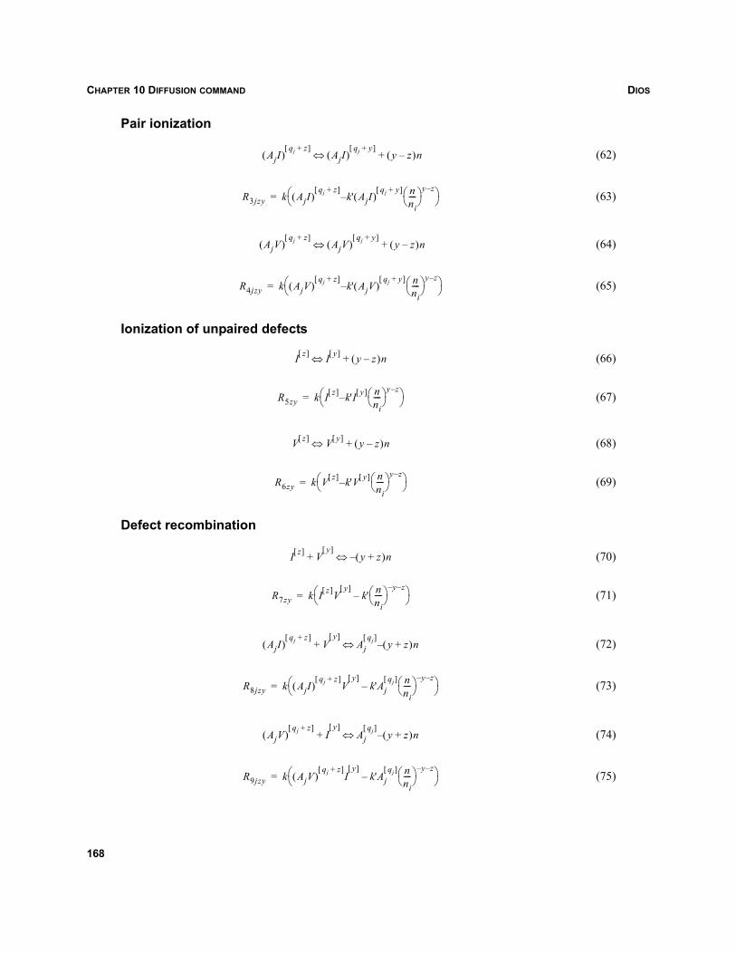
DIOSCHAPTER 10 DIFFUSION COMMAND
Pair ionization
(62)
(63)
(64)
(65)
Ionization of unpaired defects
(66)
(67)
(68)
(69)
Defect recombination
(70)
(71)
(72)
(73)
(74)
(75)
AjI( )qj z+[ ]
AjI( )qj y+[ ]
y z–( )n+⇔
R3jzy k AjI( )qj z+[ ]
k' AjI( )–qj y+[ ] n
ni----⎝ ⎠
⎛ ⎞ y z–
⎝ ⎠⎛ ⎞=
AjV( )qj z+[ ]
AjV( )qj y+[ ]
y z–( )n+⇔
R4jzy k AjV( )qj z+[ ]
k' AjV( )–qj y+[ ] n
ni----⎝ ⎠
⎛ ⎞ y z–
⎝ ⎠⎛ ⎞=
I z[ ] I y[ ] y z–( )n+⇔
R5zy k I z[ ] k'I– y[ ] nni----⎝ ⎠
⎛ ⎞ y z–
⎝ ⎠⎛ ⎞=
V z[ ] V y[ ] y z–( )n+⇔
R6zy k V z[ ] k'V– y[ ] nni----⎝ ⎠
⎛ ⎞ y z–
⎝ ⎠⎛ ⎞=
I z[ ] V+y[ ]
y z+( )– n⇔
R7zy k I z[ ]Vy[ ]
k' nni----⎝ ⎠
⎛ ⎞ y– z––⎝ ⎠
⎛ ⎞=
AjI( )qj z+[ ]
V+y[ ]
Ajqj[ ]
y z+( )– n⇔
R8jzy k AjI( )qj z+[ ]
Vy[ ]
k'Ajqj[ ] n
ni----⎝ ⎠
⎛ ⎞ y– z––⎝ ⎠
⎛ ⎞=
AjV( )qj z+[ ]
I+y[ ]
Ajqj[ ]
y z+( )– n⇔
R9jzy k AjV( )qj z+[ ]
Iy[ ]
k'Ajqj[ ] n
ni----⎝ ⎠
⎛ ⎞ y– z––⎝ ⎠
⎛ ⎞=
168
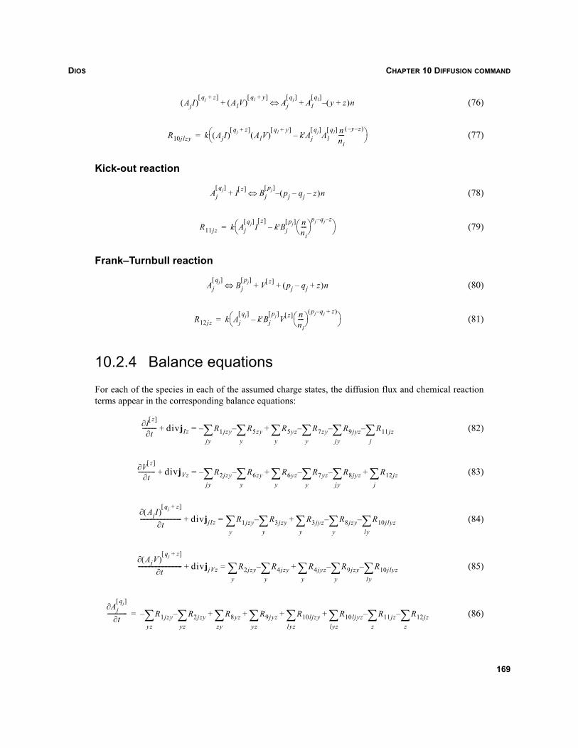
DIOS CHAPTER 10 DIFFUSION COMMAND
(76)
(77)
Kick-out reaction
(78)
(79)
Frank–Turnbull reaction
(80)
(81)
10.2.4 Balance equations
For each of the species in each of the assumed charge states, the diffusion flux and chemical reactionterms appear in the corresponding balance equations:
(82)
(83)
(84)
(85)
(86)
AjI( )qj z+[ ]
AlV( )ql y+[ ]
+ Ajqj[ ]
Alql[ ]
y z+( )– n+⇔
R10jlzy k AjI( )qj z+[ ]
AlV( )ql y+[ ]
k'Ajqj[ ]
Alql[ ] n
ni----
y– z–( )–⎝ ⎠
⎛ ⎞=
Ajqj[ ]
I z[ ]+ Bjpj[ ]
pj qj– z–( )– n⇔
R11 jz k Ajqj[ ]
Iz[ ]
k'Bjpj[ ] n
ni----⎝ ⎠
⎛ ⎞pj qj– z–
–⎝ ⎠⎛ ⎞=
Ajqj[ ]
Bjpj[ ]
V z[ ] pj qj– z+( )n+ +⇔
R12 jz k Ajqj[ ]
k'Bjpj[ ]
V z[ ] nni----⎝ ⎠
⎛ ⎞pj qj– z+( )
–⎝ ⎠⎛ ⎞=
I z[ ]∂t∂
---------- divjIz R1jzy R5zy R5yz R7zyy∑–
y∑ R9jyz
jy∑– R11 jz
j∑–+
y∑–
jy∑–=+
V z[ ]∂t∂
------------ divjVz R2jzy R6zy R6yz R7yzy∑–
y∑ R8jyz
jy∑– R12 jz
j∑+ +
y∑–
jy∑–=+
AjI( )qj z+[ ]
∂t∂
----------------------------- divjjIz R1 jzy R3jzy R3jyz R8jzyy∑–
y∑ R10 jlyz
ly∑–+
y∑–
y∑=+
AjV( )qj z+[ ]
∂t∂
------------------------------- divjjVz R2 jzy R4jzy R4jyz R9jzyy∑–
y∑ R10 jlyz
ly∑–+
y∑–
y∑=+
Ajqj[ ]
∂t∂
-------------- R1jzy R2jzy R8yz R9jyzyz∑+
zy∑ R10ljzy
lyz∑ R10ljyz R11jz R12jz
z∑–
z∑–
lyz∑+ + +
yz∑–
yz∑–=
169
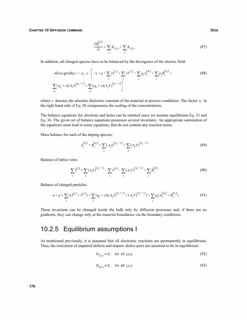
DIOSCHAPTER 10 DIFFUSION COMMAND
(87)
In addition, all charged species have to be balanced by the divergence of the electric field:
(88)
where denotes the absolute dielectric constant of the material at process conditions. The factor inthe right hand side of Eq. 88 compensates the scaling of the concentrations.
The balance equations for electrons and holes can be omitted since we assume equilibrium Eq. 35 andEq. 36. The given set of balance equations possesses several invariants. An appropriate summation ofthe equations must lead to some equations, that do not contain any reaction terms.
Mass balance for each of the doping species:
(89)
Balance of lattice sites:
(90)
Balance of charged particles:
(91)
These invariants can be changed inside the bulk only by diffusion processes and, if there are nogradients, they can change only at the material boundaries via the boundary conditions.
10.2.5 Equilibrium assumptions I
As mentioned previously, it is assumed that all electronic reactions are permanently in equilibrium.Thus, the ionization of unpaired defects and dopant–defect pairs are assumed to be in equilibrium:
(92)
(93)
Bjpj[ ]
∂t∂
-------------- R11jzz
∑= R12jzz
∑+
div εgradϕ( )– ni e n– p zI z[ ] zV z[ ] qjAjqj[ ]
j∑ pjBj
pj[ ]
j∑
qj z+( ) AjI( )qj z+[ ]
jz∑ qj z+( ) AjV( )
qj z+[ ]
jz∑
+ + +
+
z∑+
z∑+ +⋅ ⋅=
ε ni
Ajqj[ ]
Bjpj[ ]
AjI( )qj z+[ ]
z∑ AjV( )
qj z+[ ]
z∑+ + +
I z[ ]
z∑ AjI( )
qj z+[ ]
z∑ V z[ ]
z∑ AjV( )
qj z+[ ]
z∑–– Bj
p[ ]j
j∑+ +
n p z I z[ ] V z[ ]+( )z
∑+ +– qj z+( ) AjI( )qj z+[ ]
AjV( )qj z+[ ]
+( )z
∑ qj Ajqj[ ]
Bjpj[ ]
+( )j
∑+ +
R3jzy 0 for all j,z,y,≡
R4jzy 0 for all j,z,y,≡
170
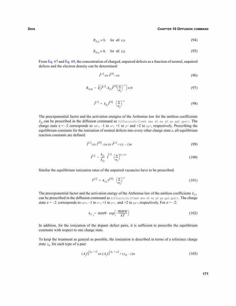
DIOS CHAPTER 10 DIFFUSION COMMAND
(94)
(95)
From Eq. 67 and Eq. 69, the concentration of charged, unpaired defects as a function of neutral, unpaireddefects and the electron density can be determined:
(96)
(97)
(98)
The preexponential factor and the activation energies of the Arrhenius law for the unitless coefficientscan be prescribed in the diffusion command as Diffusion(Si(I(mm0 mmw m0 mw p0 pw pp0 ppw)). The
charge state z = –2 corresponds to mm*, –1 to m*, +1 to p* and +2 to pp*, respectively. Prescribing theequilibrium constants for the ionization of neutral defects into every other charge state z, all equilibriumreaction constants are defined:
(99)
(100)
Similar the equilibrium ionization rates of the unpaired vacancies have to be prescribed:
(101)
The preexponential factor and the activation energy of the Arrhenius law of the unitless coefficients can be prescribed in the diffusion command as Diffusion(Si(V(mm0 mmw m0 mw p0 pw pp0 ppw)). The chargestate z = –2 corresponds to mm*, –1 to m*, +1 to p*, and +2 to pp*, respectively. For z = –2:
(102)
In addition, for the ionization of the dopant–defect pairs, it is sufficient to prescribe the equilibriumconstants with respect to one charge state.
To keep the treatment as general as possible, the ionization is described in terms of a reference chargestate for each type of a pair:
(103)
R5zy 0 for all z,y,≡
R6zy 0 for all z,y,≡
I z[ ] I 0[ ] z– n⇔
R5z0 k I z[ ] kIzI– 0[ ] nni----⎝ ⎠
⎛ ⎞ z–
⎝ ⎠⎛ ⎞ 0≡=
I z[ ] kIzI0[ ] n
ni----⎝ ⎠
⎛ ⎞ z–=
kIz
I z[ ] I 0[ ] z– n I y[ ] y z–( )n+⇔⇔
I z[ ] kIzkIy------ I
y[ ] n
ni----⎝ ⎠
⎛ ⎞ y z–( )=
V z[ ] kVzV0[ ] n
ni----⎝ ⎠
⎛ ⎞ z–=
kVz
kV 2–mm0 mmw
kT----------------–⎝ ⎠
⎛ ⎞exp⋅=
z0
AjI( )qj z+[ ]
AjI( )qj z0+[ ]
z0 z–( )n+⇔
171
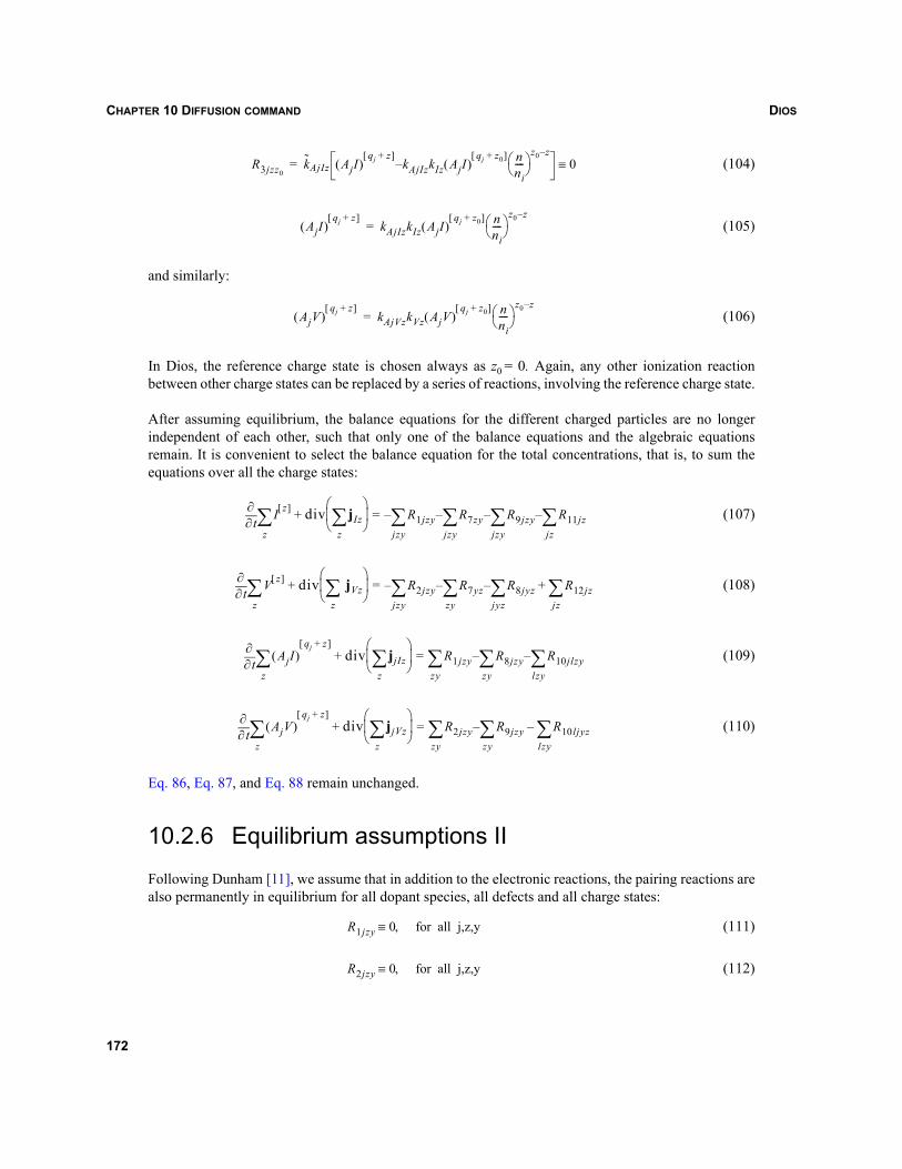
DIOSCHAPTER 10 DIFFUSION COMMAND
(104)
(105)
and similarly:
(106)
In Dios, the reference charge state is chosen always as z0 = 0. Again, any other ionization reactionbetween other charge states can be replaced by a series of reactions, involving the reference charge state.
After assuming equilibrium, the balance equations for the different charged particles are no longerindependent of each other, such that only one of the balance equations and the algebraic equationsremain. It is convenient to select the balance equation for the total concentrations, that is, to sum theequations over all the charge states:
(107)
(108)
(109)
(110)
Eq. 86, Eq. 87, and Eq. 88 remain unchanged.
10.2.6 Equilibrium assumptions II
Following Dunham [11], we assume that in addition to the electronic reactions, the pairing reactions arealso permanently in equilibrium for all dopant species, all defects and all charge states:
(111)
(112)
R3jzz0kAjIz AjI( )
qj z+[ ]kAjIzkIz AjI( )
qj z0+[ ]– n
ni----⎝ ⎠
⎛ ⎞z0 z–
0≡=
AjI( )qj z+[ ]
kAjIzkIz AjI( )qj z0+[ ] n
ni----⎝ ⎠
⎛ ⎞z0 z–
=
AjV( )qj z+[ ]
kAjVzkVz AjV( )qj z0+[ ] n
ni----⎝ ⎠
⎛ ⎞z0 z–
=
t∂∂ I z[ ]
z∑ div jIz
z∑⎝ ⎠
⎜ ⎟⎛ ⎞
R1jzyjzy∑ R7zy
jzy∑– R9 jzy
jzy∑– R11jz
jz∑––=+
t∂∂ V z[ ]
z∑ div jVz
z∑⎝ ⎠
⎜ ⎟⎛ ⎞
R2jzyjzy∑ R7yz
zy∑– R8 jyz
jyz∑– R12jz
jz∑+–=+
t∂∂ AjI( )
z∑
qj z+[ ]div jjIz
z∑⎝ ⎠
⎜ ⎟⎛ ⎞
R1 jzy R8jzy R10 jlzylzy∑–
zy∑–
zy∑=+
t∂∂ AjV( )
z∑
qj z+[ ]div jjVz
z∑⎝ ⎠
⎜ ⎟⎛ ⎞
R2jzy R9jzy R10ljyzlzy∑–
zy∑–
zy∑=+
R1jzy 0 for all j,z,y,≡
R2jzy 0 for all j,z,y,≡
172
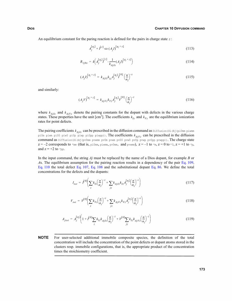
DIOS CHAPTER 10 DIFFUSION COMMAND
An equilibrium constant for the paring reaction is defined for the pairs in charge state :
(113)
(114)
(115)
and similarly:
(116)
where and denote the pairing constants for the dopant with defects in the various chargestates. These properties have the unit [cm3]. The coefficients and are the equilibrium ionizationrates for point defects.
The pairing coefficients can be prescribed in the diffusion command as Diffusion(Si(Aj(pi0mm piwmmpi0m piwm pi00 piw0 pi0p piwp pi0pp piwpp)). The coefficients can be prescribed in the diffusioncommand as Diffusion(Si(Aj(pv0mm pvwmm pv0m pvwm pv00 pvw0 pv0p pvwp pv0pp pvwpp)). The charge statez = –2 corresponds to *mm (that is, pi0mm, piwmm, pv0mm, and pvwmm), z = –1 to *m, z = 0 to *0, z = +1 to *p,and z = +2 to *pp.
In the input command, the string Aj must be replaced by the name of a Dios dopant, for example B orAs. The equilibrium assumption for the pairing reaction results in a dependency of the pair Eq. 109,Eq. 110 the total defect Eq. 107, Eq. 108 and the substitutional dopant Eq. 86. We define the totalconcentrations for the defects and the dopants:
(117)
(118)
(119)
NOTE For user-selected additional immobile composite species, the definition of the totalconcentration will include the concentration of the point defects or dopant atoms stored in theclusters resp. immobile configurations, that is, the appropriate product of the concentrationtimes the stoichiometry coefficient.
z
Ajqj[ ]
I z[ ]+ AjI( )qj z+[ ]
⇔
R1j0z k Ajqj[ ]
Iz[ ] 1
kAjIz-----------– AjI( )
qj z+[ ]
⎝ ⎠⎛ ⎞=
AjI( )qj z+[ ]
kAjIzkIzAjqj[ ]
I0[ ]
nni----⎝ ⎠
⎛ ⎞ z–=
AjV( )qj z+[ ]
kAjVzkVzAjqj[ ]
V0[ ]
nni----⎝ ⎠
⎛ ⎞ z–=
kAjIz kAjVzkIz kVz
kAjIzkAjVz
Itot I 0[ ] kIznni----⎝ ⎠
⎛ ⎞ z–kAjIzkIzAj
qj[ ] nni----⎝ ⎠
⎛ ⎞ z–
jz∑+
z∑⎝ ⎠
⎜ ⎟⎛ ⎞
=
Vtot V 0[ ] kVznni----⎝ ⎠
⎛ ⎞ z–kAjVzkVzAj
qj[ ] nni----⎝ ⎠
⎛ ⎞ z–
jz∑+
z∑⎝ ⎠
⎜ ⎟⎛ ⎞
=
Ajtot Ajqj[ ]
1 I 0[ ] kIzkAjIznni----⎝ ⎠
⎛ ⎞ z–V 0[ ] kIzkAjVz
nni----⎝ ⎠
⎛ ⎞ z–
jz∑+
z∑+
⎝ ⎠⎜ ⎟⎛ ⎞
=
173
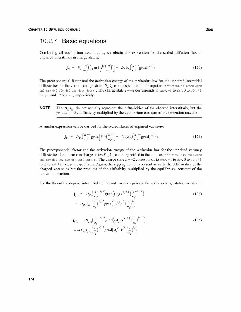
DIOSCHAPTER 10 DIFFUSION COMMAND
10.2.7 Basic equations
Combining all equilibrium assumptions, we obtain this expression for the scaled diffusion flux ofunpaired interstitials in charge state z:
(120)
The preexponential factor and the activation energy of the Arrhenius law for the unpaired interstitialdiffusivities for the various charge states can be specified in the input as Diffusion(Si(I(dmm0 dmmwdm0 dmw d00 d0w dp0 dpw dpp0 dppw)). The charge state z = –2 corresponds to dmm*, –1 to dm*, 0 to d0*, +1to dp*, and +2 to dpp*, respectively.
NOTE The do not actually represent the diffusivities of the charged interstitials, but theproduct of the diffusivity multiplied by the equilibrium constant of the ionization reaction.
A similar expression can be derived for the scaled fluxes of unpaired vacancies:
(121)
The preexponential factor and the activation energy of the Arrhenius law for the unpaired vacancydiffusivities for the various charge states can be specified in the input as Diffusion(Si(V(dmm0 dmmwdm0 dmw d00 d0w dp0 dpw dpp0 dppw)). The charge state z = –2 corresponds to dmm*, –1 to dm*, 0 to d0*, +1to dp*, and +2 to dpp*, respectively. Again, the do not represent actually the diffusivities of thecharged vacancies but the products of the diffusivity multiplied by the equilibrium constant of theionization reaction.
For the flux of the dopant–interstitial and dopant–vacancy pairs in the various charge states, we obtain:
(122)
(123)
jIz DIznni----⎝ ⎠
⎛ ⎞ z–grad I z[ ] n
ni----⎝ ⎠
⎛ ⎞ zDIzkIz
nni----⎝ ⎠
⎛ ⎞–z–grad I 0[ ]( )=–=
DIzkIz
DIzkIz
jVz DVznni----⎝ ⎠
⎛ ⎞ z–grad V z[ ] n
ni----⎝ ⎠
⎛ ⎞ zDVzkVz
nni----⎝ ⎠
⎛ ⎞–z–grad V 0[ ]( )=–=
DVzkVz
DVzkVz
jjIz DjIznni----⎝ ⎠
⎛ ⎞qj z––
grad AjI( )qj z+[ ] n
ni----⎝ ⎠
⎛ ⎞qj z+
⎝ ⎠⎛ ⎞
DjIzkjIznni----⎝ ⎠
⎛ ⎞qj z––
– grad Ajqj[ ]
I0[ ] n
ni----⎝ ⎠
⎛ ⎞qj
⎝ ⎠⎛ ⎞=
–=
jjVz DjVznni----⎝ ⎠
⎛ ⎞qj z––
grad AjV( )qj z+[ ] n
ni----⎝ ⎠
⎛ ⎞qj z+
⎝ ⎠⎛ ⎞
DjVzkjVznni----⎝ ⎠
⎛ ⎞qj z––
– grad Ajqj[ ]
V0[ ] n
ni----⎝ ⎠
⎛ ⎞qj
⎝ ⎠⎛ ⎞=
–=
174
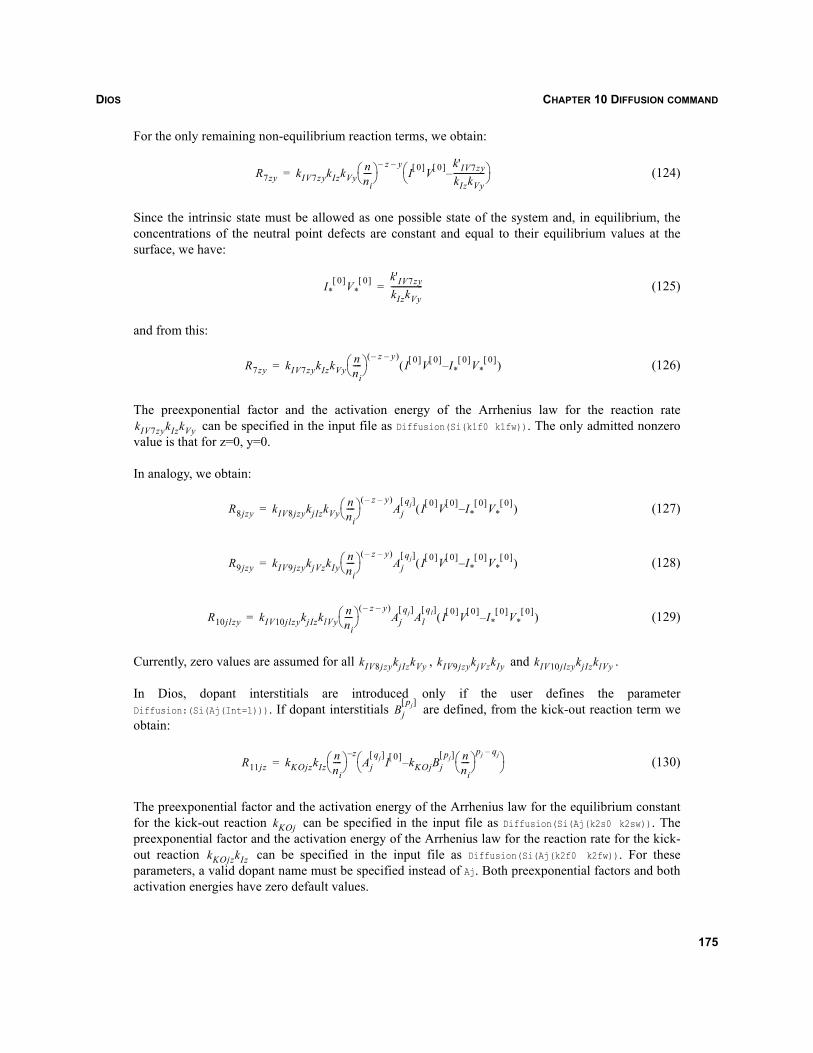
DIOS CHAPTER 10 DIFFUSION COMMAND
For the only remaining non-equilibrium reaction terms, we obtain:
(124)
Since the intrinsic state must be allowed as one possible state of the system and, in equilibrium, theconcentrations of the neutral point defects are constant and equal to their equilibrium values at thesurface, we have:
(125)
and from this:
(126)
The preexponential factor and the activation energy of the Arrhenius law for the reaction rate can be specified in the input file as Diffusion(Si(k1f0 k1fw)). The only admitted nonzero
value is that for z=0, y=0.
In analogy, we obtain:
(127)
(128)
(129)
Currently, zero values are assumed for all , and .
In Dios, dopant interstitials are introduced only if the user defines the parameterDiffusion:(Si(Aj(Int=1))). If dopant interstitials are defined, from the kick-out reaction term weobtain:
(130)
The preexponential factor and the activation energy of the Arrhenius law for the equilibrium constantfor the kick-out reaction can be specified in the input file as Diffusion(Si(Aj(k2s0 k2sw)). Thepreexponential factor and the activation energy of the Arrhenius law for the reaction rate for the kick-out reaction can be specified in the input file as Diffusion(Si(Aj(k2f0 k2fw)). For theseparameters, a valid dopant name must be specified instead of Aj. Both preexponential factors and bothactivation energies have zero default values.
R7zy kIV7zykIzkVynni----⎝ ⎠
⎛ ⎞ z– y–I 0[ ]V 0[ ] k'IV7zy
kIzkVy----------------–⎝ ⎠
⎛ ⎞=
I*0[ ]V*
0[ ] k'IV7zykIzkVy----------------=
R7zy kIV7zykIzkVynni----⎝ ⎠
⎛ ⎞ z– y–( )I 0[ ]V 0[ ] I*
0[ ]V*0[ ]–( )=
kIV7zykIzkVy
R8 jzy kIV8 jzykjIzkVynni----⎝ ⎠
⎛ ⎞ z– y–( )Aj
qj[ ]I 0[ ]V 0[ ] I*
0[ ]V*0[ ]–( )=
R9 jzy kIV9 jzykjVzkIynni----⎝ ⎠
⎛ ⎞ z– y–( )Aj
qj[ ]I 0[ ]V 0[ ] I*
0[ ]V*0[ ]–( )=
R10 jlzy kIV10jlzykjIzklVynni----⎝ ⎠
⎛ ⎞ z– y–( )Aj
qj[ ]Al
ql[ ]I 0[ ]V 0[ ] I*
0[ ]V*0[ ]–( )=
kIV8jzykjIzkVy kIV9 jzykjVzkIy kIV10 jlzykjIzklVy
Bjpj[ ]
R11jz kKOjzkIznni----⎝ ⎠
⎛ ⎞ z–Aj
qj[ ]I 0[ ] kKOjBj
pj[ ] nni----⎝ ⎠
⎛ ⎞pj qj–
–⎝ ⎠⎛ ⎞=
kKOj
kKOjzkIz
175
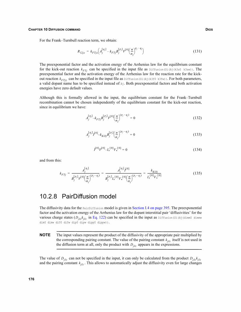
DIOSCHAPTER 10 DIFFUSION COMMAND
For the Frank–Turnbull reaction term, we obtain:
(131)
The preexponential factor and the activation energy of the Arrhenius law for the equilibrium constantfor the kick-out reaction can be specified in the input file as Diffusion(Si(Aj(k3s0 k3sw)). Thepreexponential factor and the activation energy of the Arrhenius law for the reaction rate for the kick-out reaction can be specified in the input file as Diffusion(Si(Aj(k3f0 k3fw)). For both parameters,a valid dopant name has to be specified instead of Aj. Both preexponential factors and both activationenergies have zero default values.
Although this is formally allowed in the input, the equilibrium constant for the Frank–Turnbullrecombination cannot be chosen independently of the equilibrium constant for the kick-out reaction,since in equilibrium we have:
(132)
(133)
(134)
and from this:
(135)
10.2.8 PairDiffusion model
The diffusivity data for the PairDiffusion model is given in Section I.4 on page 395. The preexponentialfactor and the activation energy of the Arrhenius law for the dopant interstitial pair ‘diffusivities’ for thevarious charge states ( in Eq. 122) can be specified in the input as Diffusion(Si(Aj(dimm0 dimmwdim0 dimw di00 di0w dip0 dipw dipp0 dippw)).
NOTE The input values represent the product of the diffusivity of the appropriate pair multiplied bythe corresponding pairing constant. The value of the pairing constant itself is not used inthe diffusion term at all, only the product with appears in the expressions.
The value of can not be specified in the input, it can only be calculated from the product and the pairing constant . This allows to automatically adjust the diffusivity even for large changes
R12jz kFTjz Ajqj[ ]
kFTjBjpj[ ]
V 0[ ] nni----⎝ ⎠
⎛ ⎞pj qj–
–⎝ ⎠⎛ ⎞=
kFTj
kFTjz
Ajqj[ ]
kFTjBjpj[ ]
V 0[ ] nni----⎝ ⎠
⎛ ⎞pj qj–( )
0=–
Ajqj[ ]
I 0[ ] kKOjBjpj[ ] n
ni----⎝ ⎠
⎛ ⎞pj qj–( )
0=–
I 0[ ]V 0[ ] I*0[ ]V*
0[ ] 0=–
kFTjAj
qj[ ]
Bjpj[ ]
V 0[ ] nni----⎝ ⎠
⎛ ⎞pj qj–( )
-----------------------------------------------Aj
qj[ ]I 0[ ]
Bjpj[ ]
I*0[ ]V*
0[ ] nni----⎝ ⎠
⎛ ⎞pj qj–( )
-------------------------------------------------------------kKOj
I*0[ ]V*
0[ ]-----------------------= = =
DjIzkjIz
kjIzDjIz
DjIz DjIzkjIzkjIz
176
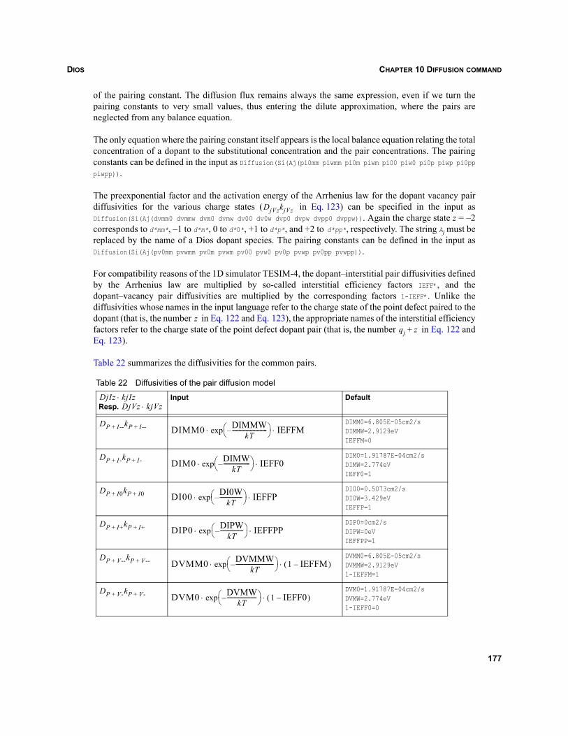
DIOS CHAPTER 10 DIFFUSION COMMAND
of the pairing constant. The diffusion flux remains always the same expression, even if we turn thepairing constants to very small values, thus entering the dilute approximation, where the pairs areneglected from any balance equation.
The only equation where the pairing constant itself appears is the local balance equation relating the totalconcentration of a dopant to the substitutional concentration and the pair concentrations. The pairingconstants can be defined in the input as Diffusion(Si(Aj(pi0mm piwmm pi0m piwm pi00 piw0 pi0p piwp pi0pppiwpp)).
The preexponential factor and the activation energy of the Arrhenius law for the dopant vacancy pairdiffusivities for the various charge states ( in Eq. 123) can be specified in the input asDiffusion(Si(Aj(dvmm0 dvmmw dvm0 dvmw dv00 dv0w dvp0 dvpw dvpp0 dvppw)). Again the charge state z = –2corresponds to d*mm*, –1 to d*m*, 0 to d*0*, +1 to d*p*, and +2 to d*pp*, respectively. The string Aj must bereplaced by the name of a Dios dopant species. The pairing constants can be defined in the input asDiffusion(Si(Aj(pv0mm pvwmm pv0m pvwm pv00 pvw0 pv0p pvwp pv0pp pvwpp)).
For compatibility reasons of the 1D simulator TESIM-4, the dopant–interstitial pair diffusivities definedby the Arrhenius law are multiplied by so-called interstitial efficiency factors IEFF*, and thedopant–vacancy pair diffusivities are multiplied by the corresponding factors 1-IEFF*. Unlike thediffusivities whose names in the input language refer to the charge state of the point defect paired to thedopant (that is, the number in Eq. 122 and Eq. 123), the appropriate names of the interstitial efficiencyfactors refer to the charge state of the point defect dopant pair (that is, the number in Eq. 122 andEq. 123).
Table 22 summarizes the diffusivities for the common pairs.
Table 22 Diffusivities of the pair diffusion model
Resp.
Input Default
DIMM0=6.805E-05cm2/sDIMMW=2.9129eVIEFFM=0
DIM0=1.91787E-04cm2/sDIMW=2.774eVIEFF0=1
DI00=0.5073cm2/sDI0W=3.429eVIEFFP=1
DIP0=0cm2/sDIPW=0eVIEFFPP=1
DVMM0=6.805E-05cm2/sDVMMW=2.9129eV1-IEFFM=1
DVM0=1.91787E-04cm2/sDVMW=2.774eV1-IEFF0=0
DjVzkjVz
zqj z+
DjIz kjIz⋅DjVz kjVz⋅
DP I--+ kP I--+ DIMM0 exp⋅ DIMMWkT
-------------------------–⎝ ⎠⎛ ⎞ IEFFM⋅
DP I-+ kP I-+ DIM0 exp⋅ DIMWkT
-------------------–⎝ ⎠⎛ ⎞ IEFF0⋅
DP I0+ kP I0+ DI00 exp⋅ DI0WkT
----------------–⎝ ⎠⎛ ⎞ IEFFP⋅
DP I++ kP I++ DIP0 exp⋅ DIPWkT
-----------------–⎝ ⎠⎛ ⎞ IEFFPP⋅
DP V--+ kP V--+ DVMM0 exp⋅ DVMMWkT
---------------------------–⎝ ⎠⎛ ⎞ 1 IEFFM–( )⋅
DP V-+ kP V-+ DVM0 exp⋅ DVMWkT
---------------------–⎝ ⎠⎛ ⎞ 1 IEFF0–( )⋅
177
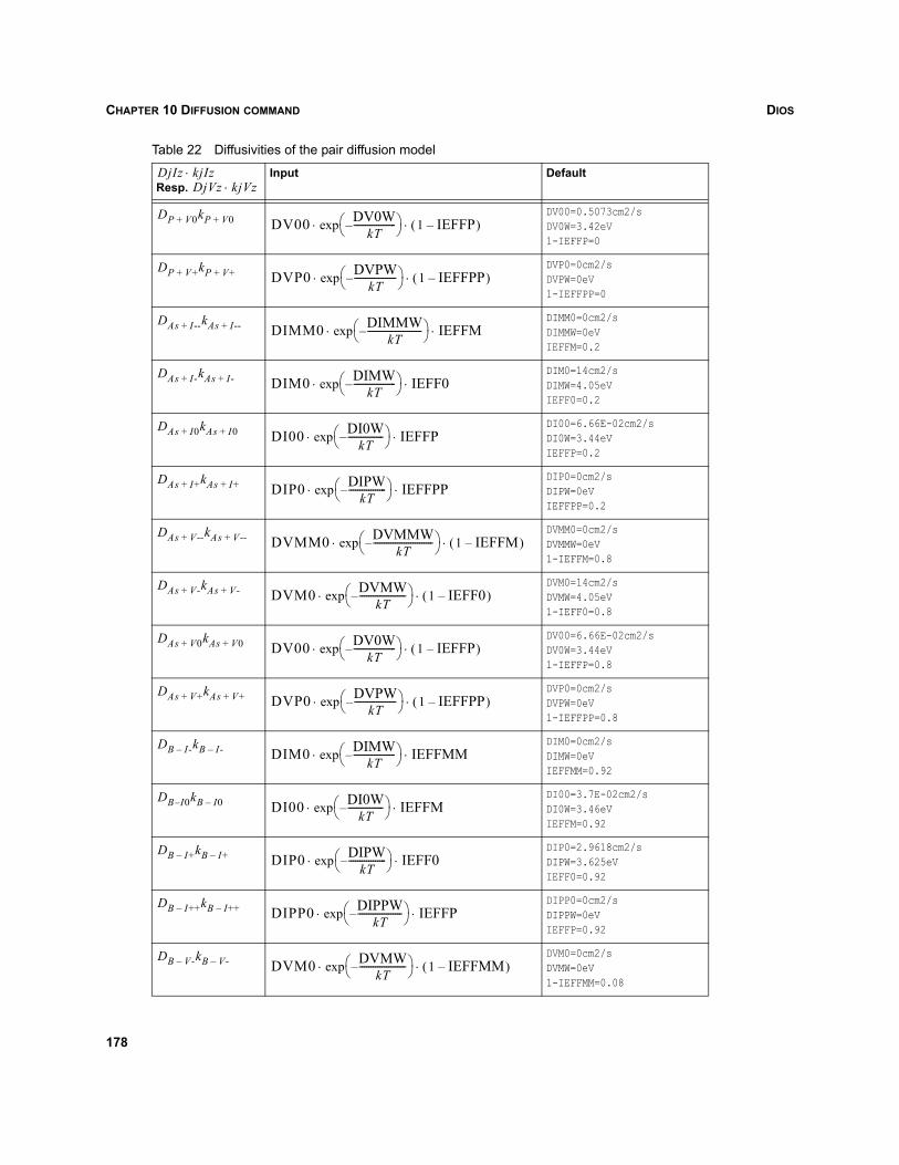
DIOSCHAPTER 10 DIFFUSION COMMAND
DV00=0.5073cm2/sDV0W=3.42eV1-IEFFP=0
DVP0=0cm2/sDVPW=0eV1-IEFFPP=0
DIMM0=0cm2/sDIMMW=0eVIEFFM=0.2
DIM0=14cm2/sDIMW=4.05eVIEFF0=0.2
DI00=6.66E-02cm2/sDI0W=3.44eVIEFFP=0.2
DIP0=0cm2/sDIPW=0eVIEFFPP=0.2
DVMM0=0cm2/sDVMMW=0eV1-IEFFM=0.8
DVM0=14cm2/sDVMW=4.05eV1-IEFF0=0.8
DV00=6.66E-02cm2/sDV0W=3.44eV1-IEFFP=0.8
DVP0=0cm2/sDVPW=0eV1-IEFFPP=0.8
DIM0=0cm2/sDIMW=0eVIEFFMM=0.92
DI00=3.7E-02cm2/sDI0W=3.46eVIEFFM=0.92
DIP0=2.9618cm2/sDIPW=3.625eVIEFF0=0.92
DIPP0=0cm2/sDIPPW=0eVIEFFP=0.92
DVM0=0cm2/sDVMW=0eV1-IEFFMM=0.08
Table 22 Diffusivities of the pair diffusion model
Resp.
Input DefaultDjIz kjIz⋅DjVz kjVz⋅
DP V0+ kP V0+ DV00 exp⋅ DV0WkT
-------------------–⎝ ⎠⎛ ⎞ 1 IEFFP–( )⋅
DP V++ kP V++ DVP0 exp⋅ DVPWkT
-------------------–⎝ ⎠⎛ ⎞ 1 IEFFPP–( )⋅
DAs I--+ kAs I--+ DIMM0 exp⋅ DIMMWkT
-------------------------–⎝ ⎠⎛ ⎞ IEFFM⋅
DAs I-+ kAs I-+ DIM0 exp⋅ DIMWkT
-------------------–⎝ ⎠⎛ ⎞ IEFF0⋅
DAs I0+ kAs I0+ DI00 exp⋅ DI0WkT
----------------–⎝ ⎠⎛ ⎞ IEFFP⋅
DAs I++ kAs I++ DIP0 exp⋅ DIPWkT
-----------------–⎝ ⎠⎛ ⎞ IEFFPP⋅
DAs V--+ kAs V--+ DVMM0 exp⋅ DVMMWkT
---------------------------–⎝ ⎠⎛ ⎞ 1 IEFFM–( )⋅
DAs V-+ kAs V-+ DVM0 exp⋅ DVMWkT
---------------------–⎝ ⎠⎛ ⎞ 1 IEFF0–( )⋅
DAs V0+ kAs V0+ DV00 exp⋅ DV0WkT
-------------------–⎝ ⎠⎛ ⎞ 1 IEFFP–( )⋅
DAs V++ kAs V++ DVP0 exp⋅ DVPWkT
-------------------–⎝ ⎠⎛ ⎞ 1 IEFFPP–( )⋅
DB I-– kB I-– DIM0 exp⋅ DIMWkT
-------------------–⎝ ⎠⎛ ⎞ IEFFMM⋅
DB I– 0kB I0– DI00 exp⋅ DI0WkT
----------------–⎝ ⎠⎛ ⎞ IEFFM⋅
DB I+– kB I+– DIP0 exp⋅ DIPWkT
-----------------–⎝ ⎠⎛ ⎞ IEFF0⋅
DB I++– kB I++– DIPP0 exp⋅ DIPPWkT
--------------------–⎝ ⎠⎛ ⎞ IEFFP⋅
DB V-– kB V-– DVM0 exp⋅ DVMWkT
---------------------–⎝ ⎠⎛ ⎞ 1 IEFFMM–( )⋅
178
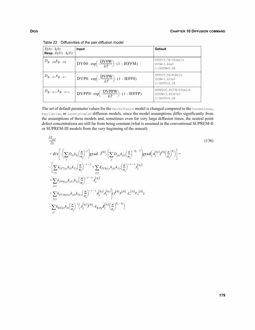
DIOS CHAPTER 10 DIFFUSION COMMAND
The set of default parameter values for the PairDiffusion model is changed compared to the Conventional,Equilibrium, or LooselyCoupled diffusion models, since the model assumptions differ significantly fromthe assumptions of these models and, sometimes even for very large diffusion times, the neutral pointdefect concentrations are still far from being constant (what is assumed in the conventional SUPREM-IIor SUPREM-III models from the very beginning of the anneal).
(136)
DV00=3.7E-02cm2/sDV0W=3.46eV1-IEFFM=0.08
DVP0=2.9618cm2/sDVPW=3.625eV1-IEFF0=0.08
DVPP0=6.9537E-03cm2/sDVPPW=3.45367eV1-IEFFP=0.08
Table 22 Diffusivities of the pair diffusion model
Resp.
Input DefaultDjIz kjIz⋅DjVz kjVz⋅
DB V0– kB V0– DV00 exp⋅ DV0WkT
-------------------–⎝ ⎠⎛ ⎞ 1 IEFFM–( )⋅
DB V+– kB V+– DVP0 exp⋅ DVPWkT
-------------------–⎝ ⎠⎛ ⎞ 1 IEFF0–( )⋅
DB V++– kB V++– DVPP0 exp⋅ DVPPWkT
-----------------------–⎝ ⎠⎛ ⎞ 1 IEFFP–( )⋅
Itot∂t∂
----------
div DIzkIznni----⎝ ⎠
⎛ ⎞ z–
z∑⎝ ⎠
⎜ ⎟⎛ ⎞
grad I 0[ ] DjIzkjIznni----⎝ ⎠
⎛ ⎞qj– z–
j∑⎝ ⎠
⎜ ⎟⎛ ⎞
grad Ajqj[ ]
I 0[ ] nni----⎝ ⎠
⎛ ⎞qj
⎝ ⎠⎛ ⎞––
kIV7zyzy∑ kIzkVy
nni----⎝ ⎠
⎛ ⎞ z– y–kIV8jzy
jzy∑ kjIzkVy
nni----⎝ ⎠
⎛ ⎞ z– y–Aj
qj[ ]
kIV9jzyjzy∑ kjVzkIy
nni----⎝ ⎠
⎛ ⎞ z– y–Aj
qj[ ]
kIV10 jlzyjzy∑ kjIzklVy
nni----⎝ ⎠
⎛ ⎞ z– y–Aj
qj[ ]Al
ql[ ]
+
+
+ I 0[ ]V 0[ ] I*0[ ]V*
0[ ]–( )
–
kKOjzkIznni----⎝ ⎠
⎛ ⎞ z–Aj
qj[ ]I 0[ ] kKOjBj
pj[ ] nni----⎝ ⎠
⎛ ⎞pj qj–
–⎝ ⎠⎛ ⎞
jz∑–
=+
179
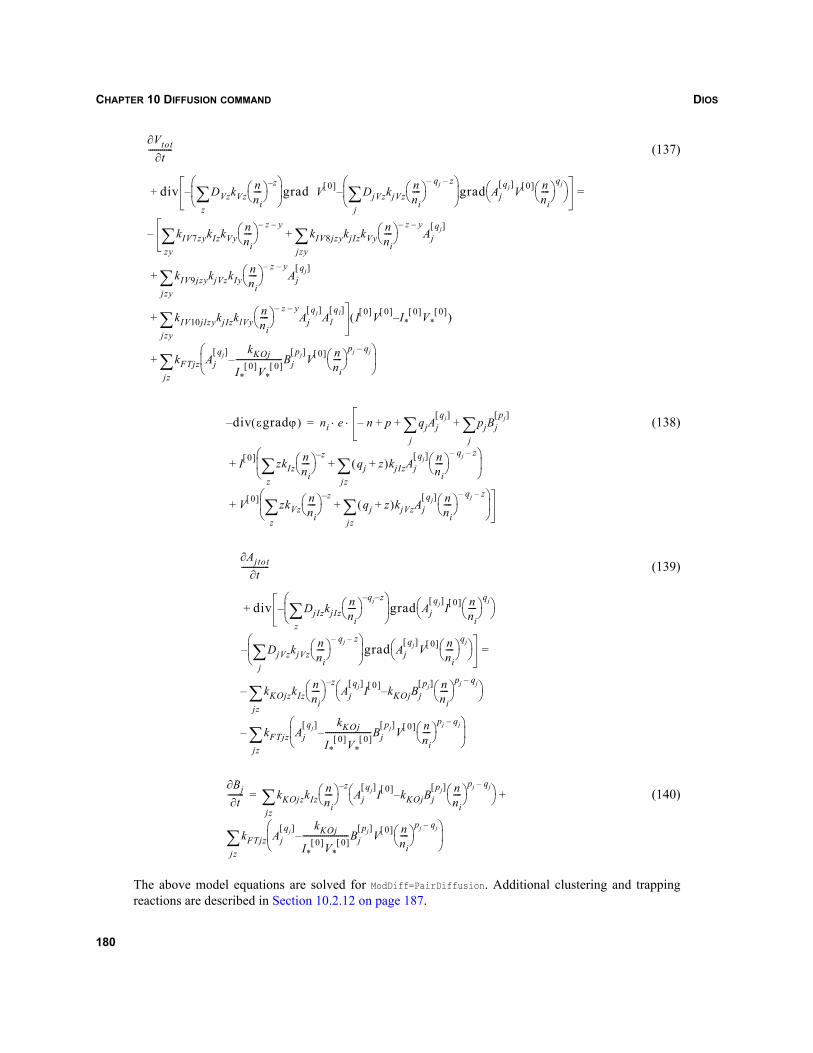
DIOSCHAPTER 10 DIFFUSION COMMAND
(137)
(138)
(139)
(140)
The above model equations are solved for ModDiff=PairDiffusion. Additional clustering and trappingreactions are described in Section 10.2.12 on page 187.
Vtot∂t∂
------------
div DVzkVznni----⎝ ⎠
⎛ ⎞ z–
z∑⎝ ⎠
⎜ ⎟⎛ ⎞
grad V 0[ ] DjVzkjVznni----⎝ ⎠
⎛ ⎞qj– z–
j∑⎝ ⎠
⎜ ⎟⎛ ⎞
grad Ajqj[ ]
V 0[ ] nni----⎝ ⎠
⎛ ⎞qj
⎝ ⎠⎛ ⎞––
kIV7zyzy∑ kIzkVy
nni----⎝ ⎠
⎛ ⎞ z– y–kIV8jzy
jzy∑ kjIzkVy
nni----⎝ ⎠
⎛ ⎞ z– y–Aj
qj[ ]
kIV9jzyjzy∑ kjVzkIy
nni----⎝ ⎠
⎛ ⎞ z– y–Aj
qj[ ]
kIV10jlzyjzy∑ kjIzklVy
nni----⎝ ⎠
⎛ ⎞ z– y–Aj
qj[ ]Al
ql[ ]
+
+
+ I 0[ ]V 0[ ] I*0[ ]V*
0[ ]–( )
–
kFTjz Ajqj[ ] kKOj
I*0[ ]V*
0[ ]-----------------------Bj
pj[ ]V 0[ ] n
ni----⎝ ⎠
⎛ ⎞pj qj–
–⎝ ⎠⎜ ⎟⎛ ⎞
jz∑+
=+
div εgradϕ( )– ni e n– p qjAjqj[ ]
j∑ pjBj
pj[ ]
j∑
I 0[ ] zkIznni----⎝ ⎠
⎛ ⎞ z–qj z+( )kjIzAj
qj[ ] nni----⎝ ⎠
⎛ ⎞qj– z–
jz∑+
z∑⎝ ⎠
⎜ ⎟⎛ ⎞
V 0[ ] zkVznni----⎝ ⎠
⎛ ⎞ z–qj z+( )kjVzAj
qj[ ] nni----⎝ ⎠
⎛ ⎞qj– z–
jz∑+
z∑⎝ ⎠
⎜ ⎟⎛ ⎞
+
+
+
+ +⋅ ⋅=
Ajtot∂t∂
--------------
div DjIzkjIznni----⎝ ⎠
⎛ ⎞qj z––
z∑⎝ ⎠
⎜ ⎟⎛ ⎞
grad Ajqj[ ]
I 0[ ] nni----⎝ ⎠
⎛ ⎞qj
⎝ ⎠⎛ ⎞
DjVzkjVznni----⎝ ⎠
⎛ ⎞qj– z–
j∑⎝ ⎠
⎜ ⎟⎛ ⎞
grad Ajqj[ ]
V 0[ ] nni----⎝ ⎠
⎛ ⎞qj
⎝ ⎠⎛ ⎞–
–
kKOjzkIznni----⎝ ⎠
⎛ ⎞ z–Aj
qj[ ]I 0[ ] kKOjBj
pj[ ] nni----⎝ ⎠
⎛ ⎞pj qj–
–⎝ ⎠⎛ ⎞
jz∑–
kFTjz Ajqj[ ] kKOj
I*0[ ]V*
0[ ]-----------------------Bj
pj[ ]V 0[ ] n
ni----⎝ ⎠
⎛ ⎞pj qj–
–⎝ ⎠⎜ ⎟⎛ ⎞
jz∑–
=
+
Bj∂t∂
-------- kKOjzkIznni----⎝ ⎠
⎛ ⎞ z–Aj
qj[ ]I 0[ ] kKOjBj
pj[ ] nni----⎝ ⎠
⎛ ⎞pj qj–
–⎝ ⎠⎛ ⎞
jz∑
kFTjz Ajqj[ ] kKOj
I*0[ ]V*
0[ ]-----------------------Bj
pj[ ]V 0[ ] n
ni----⎝ ⎠
⎛ ⎞pj qj–
–⎝ ⎠⎜ ⎟⎛ ⎞
jz∑
+=
180
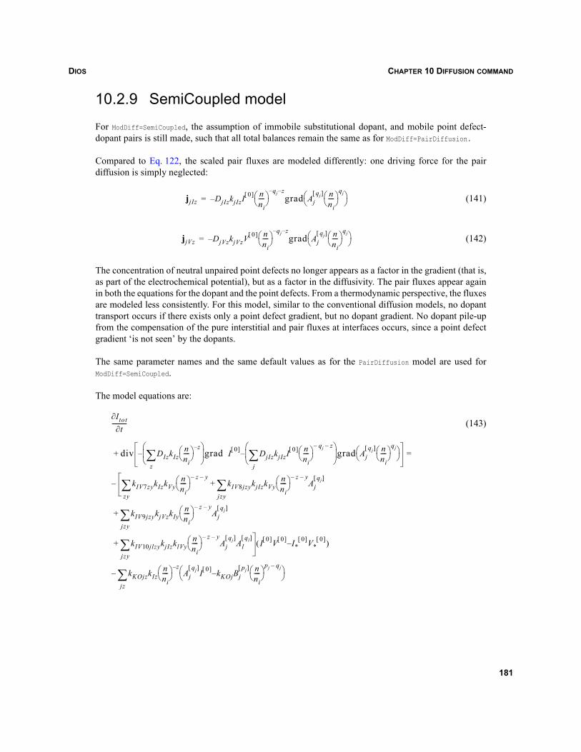
DIOS CHAPTER 10 DIFFUSION COMMAND
10.2.9 SemiCoupled model
For ModDiff=SemiCoupled, the assumption of immobile substitutional dopant, and mobile point defect-dopant pairs is still made, such that all total balances remain the same as for ModDiff=PairDiffusion.
Compared to Eq. 122, the scaled pair fluxes are modeled differently: one driving force for the pairdiffusion is simply neglected:
(141)
(142)
The concentration of neutral unpaired point defects no longer appears as a factor in the gradient (that is,as part of the electrochemical potential), but as a factor in the diffusivity. The pair fluxes appear againin both the equations for the dopant and the point defects. From a thermodynamic perspective, the fluxesare modeled less consistently. For this model, similar to the conventional diffusion models, no dopanttransport occurs if there exists only a point defect gradient, but no dopant gradient. No dopant pile-upfrom the compensation of the pure interstitial and pair fluxes at interfaces occurs, since a point defectgradient ‘is not seen’ by the dopants.
The same parameter names and the same default values as for the PairDiffusion model are used forModDiff=SemiCoupled.
The model equations are:
(143)
jjIz DjIzkjIzI0[ ] n
ni----⎝ ⎠
⎛ ⎞qj z––
– grad Ajqj[ ] n
ni----⎝ ⎠
⎛ ⎞qj
⎝ ⎠⎛ ⎞=
jjVz DjVzkjVzV 0[ ] nni----⎝ ⎠
⎛ ⎞qj z––
– grad Ajqj[ ] n
ni----⎝ ⎠
⎛ ⎞qj
⎝ ⎠⎛ ⎞=
Itot∂t∂
----------
div DIzkIznni----⎝ ⎠
⎛ ⎞ z–
z∑⎝ ⎠
⎜ ⎟⎛ ⎞
grad I 0[ ] DjIzkjIzI 0[ ] nni----⎝ ⎠
⎛ ⎞qj– z–
j∑⎝ ⎠
⎜ ⎟⎛ ⎞
grad Ajqj[ ] n
ni----⎝ ⎠
⎛ ⎞qj
⎝ ⎠⎛ ⎞––
kIV7zyzy∑ kIzkVy
nni----⎝ ⎠
⎛ ⎞ z– y–kIV8jzy
jzy∑ kjIzkVy
nni----⎝ ⎠
⎛ ⎞ z– y–Aj
qj[ ]
kIV9jzyjzy∑ kjVzkIy
nni----⎝ ⎠
⎛ ⎞ z– y–Aj
qj[ ]
kIV10 jlzyjzy∑ kjIzklVy
nni----⎝ ⎠
⎛ ⎞ z– y–Aj
qj[ ]Al
ql[ ]
+
+
+ I 0[ ]V 0[ ] I*0[ ]V*
0[ ]–( )
–
kKOjzkIznni----⎝ ⎠
⎛ ⎞ z–Aj
qj[ ]I 0[ ] kKOjBj
pj[ ] nni----⎝ ⎠
⎛ ⎞pj qj–
–⎝ ⎠⎛ ⎞
jz∑–
=+
181
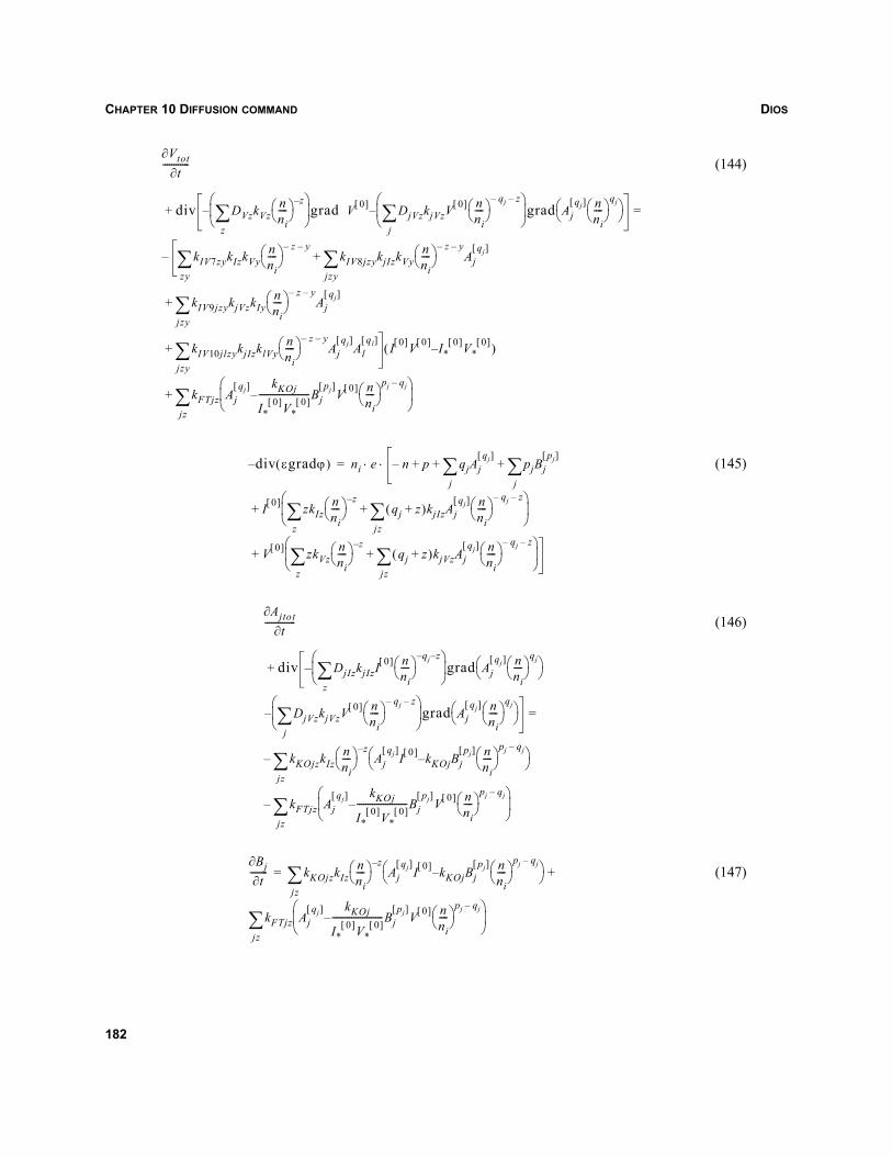
DIOSCHAPTER 10 DIFFUSION COMMAND
(144)
(145)
(146)
(147)
Vtot∂t∂
------------
div DVzkVznni----⎝ ⎠
⎛ ⎞ z–
z∑⎝ ⎠
⎜ ⎟⎛ ⎞
grad V 0[ ] DjVzkjVzV0[ ] n
ni----⎝ ⎠
⎛ ⎞qj– z–
j∑⎝ ⎠
⎜ ⎟⎛ ⎞
grad Ajqj[ ] n
ni----⎝ ⎠
⎛ ⎞qj
⎝ ⎠⎛ ⎞––
kIV7zyzy∑ kIzkVy
nni----⎝ ⎠
⎛ ⎞ z– y–kIV8jzy
jzy∑ kjIzkVy
nni----⎝ ⎠
⎛ ⎞ z– y–Aj
qj[ ]
kIV9jzyjzy∑ kjVzkIy
nni----⎝ ⎠
⎛ ⎞ z– y–Aj
qj[ ]
kIV10jlzyjzy∑ kjIzklVy
nni----⎝ ⎠
⎛ ⎞ z– y–Aj
qj[ ]Al
ql[ ]
+
+
+ I 0[ ]V 0[ ] I*0[ ]V*
0[ ]–( )
–
kFTjz Ajqj[ ] kKOj
I*0[ ]V*
0[ ]-----------------------Bj
pj[ ]V 0[ ] n
ni----⎝ ⎠
⎛ ⎞pj qj–
–⎝ ⎠⎜ ⎟⎛ ⎞
jz∑+
=+
div εgradϕ( )– ni e n– p qjAjqj[ ]
j∑ pjBj
pj[ ]
j∑
I 0[ ] zkIznni----⎝ ⎠
⎛ ⎞ z–qj z+( )kjIzAj
qj[ ] nni----⎝ ⎠
⎛ ⎞qj– z–
jz∑+
z∑⎝ ⎠
⎜ ⎟⎛ ⎞
V 0[ ] zkVznni----⎝ ⎠
⎛ ⎞ z–qj z+( )kjVzAj
qj[ ] nni----⎝ ⎠
⎛ ⎞qj– z–
jz∑+
z∑⎝ ⎠
⎜ ⎟⎛ ⎞
+
+
+
+ +⋅ ⋅=
Ajtot∂t∂
--------------
div DjIzkjIzI0[ ] n
ni----⎝ ⎠
⎛ ⎞qj z––
z∑⎝ ⎠
⎜ ⎟⎛ ⎞
grad Ajqj[ ] n
ni----⎝ ⎠
⎛ ⎞qj
⎝ ⎠⎛ ⎞
DjVzkjVzV 0[ ] nni----⎝ ⎠
⎛ ⎞qj– z–
j∑⎝ ⎠
⎜ ⎟⎛ ⎞
grad Ajqj[ ] n
ni----⎝ ⎠
⎛ ⎞qj
⎝ ⎠⎛ ⎞–
–
kKOjzkIznni----⎝ ⎠
⎛ ⎞ z–Aj
qj[ ]I 0[ ] kKOjBj
pj[ ] nni----⎝ ⎠
⎛ ⎞pj qj–
–⎝ ⎠⎛ ⎞
jz∑–
kFTjz Ajqj[ ] kKOj
I*0[ ]V*
0[ ]-----------------------Bj
pj[ ]V 0[ ] n
ni----⎝ ⎠
⎛ ⎞pj qj–
–⎝ ⎠⎜ ⎟⎛ ⎞
jz∑–
=
+
Bj∂t∂
-------- kKOjzkIznni----⎝ ⎠
⎛ ⎞ z–Aj
qj[ ]I 0[ ] kKOjBj
pj[ ] nni----⎝ ⎠
⎛ ⎞pj qj–
–⎝ ⎠⎛ ⎞
jz∑
kFTjz Ajqj[ ] kKOj
I*0[ ]V*
0[ ]-----------------------Bj
pj[ ]V 0[ ] n
ni----⎝ ⎠
⎛ ⎞pj qj–
–⎝ ⎠⎜ ⎟⎛ ⎞
jz∑
+=
182
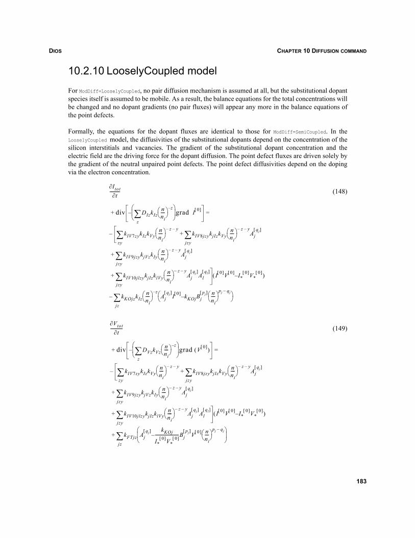
DIOS CHAPTER 10 DIFFUSION COMMAND
10.2.10 LooselyCoupled model
For ModDiff=LooselyCoupled, no pair diffusion mechanism is assumed at all, but the substitutional dopantspecies itself is assumed to be mobile. As a result, the balance equations for the total concentrations willbe changed and no dopant gradients (no pair fluxes) will appear any more in the balance equations ofthe point defects.
Formally, the equations for the dopant fluxes are identical to those for ModDiff=SemiCoupled. In theLooselyCoupled model, the diffusivities of the substitutional dopants depend on the concentration of thesilicon interstitials and vacancies. The gradient of the substitutional dopant concentration and theelectric field are the driving force for the dopant diffusion. The point defect fluxes are driven solely bythe gradient of the neutral unpaired point defects. The point defect diffusivities depend on the dopingvia the electron concentration.
(148)
(149)
Itot∂t∂
----------
div DIzkIznni----⎝ ⎠
⎛ ⎞ z–
z∑⎝ ⎠
⎜ ⎟⎛ ⎞
grad I 0[ ]–
kIV7zyzy∑ kIzkVy
nni----⎝ ⎠
⎛ ⎞ z– y–kIV8jzy
jzy∑ kjIzkVy
nni----⎝ ⎠
⎛ ⎞ z– y–Aj
qj[ ]
kIV9jzyjzy∑ kjVzkIy
nni----⎝ ⎠
⎛ ⎞ z– y–Aj
qj[ ]
kIV10jlzyjzy∑ kjIzklVy
nni----⎝ ⎠
⎛ ⎞ z– y–Aj
qj[ ]Al
ql[ ]
+
+
+ I 0[ ]V 0[ ] I*0[ ]V*
0[ ]–( )
–
kKOjzkIznni----⎝ ⎠
⎛ ⎞ z–Aj
qj[ ]I 0[ ] kKOjBj
pj[ ] nni----⎝ ⎠
⎛ ⎞pj qj–
–⎝ ⎠⎛ ⎞
jz∑–
=+
Vtot∂t∂
------------
div DVzkVznni----⎝ ⎠
⎛ ⎞ z–
z∑⎝ ⎠
⎜ ⎟⎛ ⎞
grad V 0[ ]( )–
kIV7zyzy∑ kIzkVy
nni----⎝ ⎠
⎛ ⎞ z– y–kIV8jzy
jzy∑ kjIzkVy
nni----⎝ ⎠
⎛ ⎞ z– y–Aj
qj[ ]
kIV9jzyjzy∑ kjVzkIy
nni----⎝ ⎠
⎛ ⎞ z– y–Aj
qj[ ]
kIV10jlzyjzy∑ kjIzklVy
nni----⎝ ⎠
⎛ ⎞ z– y–Aj
qj[ ]Al
ql[ ]
+
+
+ I 0[ ]V 0[ ] I*0[ ]V*
0[ ]–( )
–
kFTjz Ajqj[ ] kKOj
I*0[ ]V*
0[ ]-----------------------Bj
pj[ ]V 0[ ] n
ni----⎝ ⎠
⎛ ⎞pj qj–
–⎝ ⎠⎜ ⎟⎛ ⎞
jz∑+
=+
183
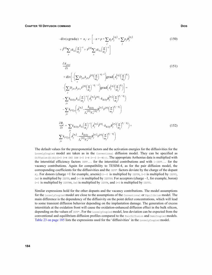
DIOSCHAPTER 10 DIFFUSION COMMAND
(150)
(151)
(152)
The default values for the preexponential factors and the activation energies for the diffusivities for theLooselyCoupled model are taken as in the Conventional diffusion model. They can be specified asDiffusion(Si(Aj(D+0 D+W DX0 DXW D-0 D-W D--0 D--W))). The appropriate Arrhenius data is multiplied withthe interstitial efficiency factors IEFF... for the interstitial contributions and with 1-IEFF... for thevacancy contributions. Again for compatibility to TESIM-4, as for the pair diffusion model, thecorresponding coefficients for the diffusivities and the IEFF* factors deviate by the charge of the dopantAj. For donors (charge +1 for example, arsenic) D--0 is multiplied by IEFFM, D-0 is multiplied by IEFF0,Dx0 is multiplied by IEFFP, and D+0 is multiplied by IEFFPP. For acceptors (charge –1, for example, boron)D-0 is multiplied by IEFFMM, Dx0 is multiplied by IEFFM, and D+0 is multiplied by IEFF0.
Similar expressions hold for the other dopants and the vacancy contributions. The model assumptionsfor the LooselyCoupled model are close to the assumptions of the Conventional or Equilibrium model. Themain difference is the dependency of the diffusivity on the point defect concentrations, which will leadto some transient diffusion behavior depending on the implantation damage. The generation of excessinterstitials at the oxidation front will cause the oxidation-enhanced diffusion effect in the bulk silicon,depending on the values of IEFF*. For the LooselyCoupled model, less deviation can be expected from theconventional and equilibrium diffusion profiles compared to the PairDiffusion and SemiCoupled models.Table 23 on page 185 lists the expressions used for the ‘diffusivities’ in the LooselyCoupled model.
div εgradϕ( )– ni e n– p qjAjqj[ ]
j∑ pjBj
pj[ ]
j∑
I 0[ ] zkIznni----⎝ ⎠
⎛ ⎞ z–
z∑ V 0[ ] zkVz
nni----⎝ ⎠
⎛ ⎞ z–
z∑
+
+ +
+ +⋅ ⋅=
Ajtot∂t∂
--------------
div DjIzkjIzI0[ ] n
ni----⎝ ⎠
⎛ ⎞qj z––
z∑⎝ ⎠
⎜ ⎟⎛ ⎞
grad Ajqj[ ] n
ni----⎝ ⎠
⎛ ⎞qj
⎝ ⎠⎛ ⎞
DjVzkjVzV 0[ ] nni----⎝ ⎠
⎛ ⎞qj– z–
j∑⎝ ⎠
⎜ ⎟⎛ ⎞
grad Ajqj[ ] n
ni----⎝ ⎠
⎛ ⎞qj
⎝ ⎠⎛ ⎞–
–
kKOjzkIznni----⎝ ⎠
⎛ ⎞ z–Aj
qj[ ]I 0[ ] kKOjBj
pj[ ] nni----⎝ ⎠
⎛ ⎞pj qj–
–⎝ ⎠⎛ ⎞
jz∑–
kFTjz Ajqj[ ] kKOj
I*0[ ]V*
0[ ]-----------------------Bj
pj[ ]V 0[ ] n
ni----⎝ ⎠
⎛ ⎞pj qj–
–⎝ ⎠⎜ ⎟⎛ ⎞
jz∑–
=
+
Bj∂t∂
-------- kKOjzkIznni----⎝ ⎠
⎛ ⎞ z–Aj
qj[ ]I 0[ ] kKOjBj
pj[ ] nni----⎝ ⎠
⎛ ⎞pj qj–
–⎝ ⎠⎛ ⎞
jz∑
kFTjz Ajqj[ ] kKOj
I*0[ ]V*
0[ ]-----------------------Bj
pj[ ]V 0[ ] n
ni----⎝ ⎠
⎛ ⎞pj qj–
–⎝ ⎠⎜ ⎟⎛ ⎞
jz∑
+=
184
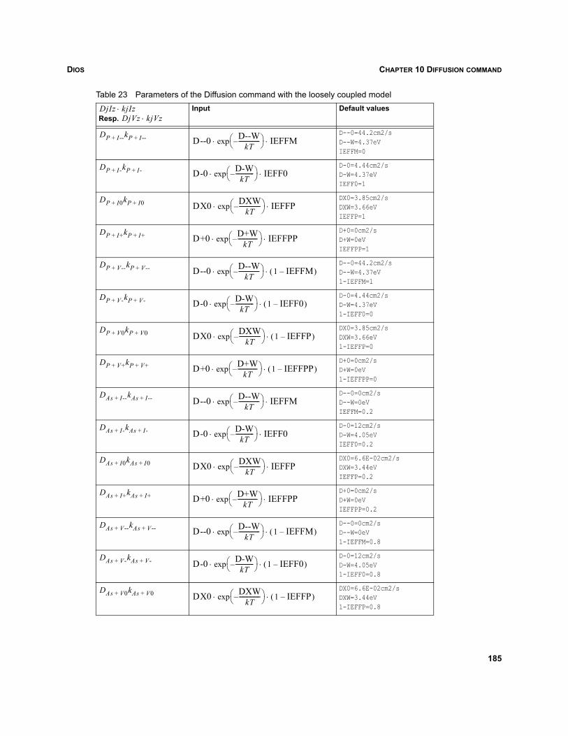
DIOS CHAPTER 10 DIFFUSION COMMAND
Table 23 Parameters of the Diffusion command with the loosely coupled model
Resp.
Input Default values
D--0=44.2cm2/sD--W=4.37eVIEFFM=0
D-0=4.44cm2/sD-W=4.37eVIEFF0=1
DX0=3.85cm2/sDXW=3.66eVIEFFP=1
D+0=0cm2/sD+W=0eVIEFFPP=1
D--0=44.2cm2/sD--W=4.37eV1-IEFFM=1
D-0=4.44cm2/sD-W=4.37eV1-IEFF0=0
DX0=3.85cm2/sDXW=3.66eV1-IEFFP=0
D+0=0cm2/sD+W=0eV1-IEFFPP=0
D--0=0cm2/sD--W=0eVIEFFM=0.2
D-0=12cm2/sD-W=4.05eVIEFF0=0.2
DX0=6.6E-02cm2/sDXW=3.44eVIEFFP=0.2
D+0=0cm2/sD+W=0eVIEFFPP=0.2
D--0=0cm2/sD--W=0eV1-IEFFM=0.8
D-0=12cm2/sD-W=4.05eV1-IEFF0=0.8
DX0=6.6E-02cm2/sDXW=3.44eV1-IEFFP=0.8
DjIz kjIz⋅DjVz kjVz⋅
DP I--+ kP I--+ D--0 exp⋅ D--WkT
---------------–⎝ ⎠⎛ ⎞ IEFFM⋅
DP I-+ kP I-+ D-0 exp⋅ D-WkT
-------------–⎝ ⎠⎛ ⎞ IEFF0⋅
DP I0+ kP I0+ DX0 exp⋅ DXWkT
---------------–⎝ ⎠⎛ ⎞ IEFFP⋅
DP I++ kP I++ D+0 exp⋅ D+WkT
--------------–⎝ ⎠⎛ ⎞ IEFFPP⋅
DP V--+ kP V--+ D--0 exp⋅ D--WkT
---------------–⎝ ⎠⎛ ⎞ 1 IEFFM–( )⋅
DP V-+ kP V-+ D-0 exp⋅ D-WkT
-------------–⎝ ⎠⎛ ⎞ 1 IEFF0–( )⋅
DP V0+ kP V0+ DX0 exp⋅ DXWkT
---------------–⎝ ⎠⎛ ⎞ 1 IEFFP–( )⋅
DP V++ kP V++ D+0 exp⋅ D+WkT
--------------–⎝ ⎠⎛ ⎞ 1 IEFFPP–( )⋅
DAs I--+ kAs I--+ D--0 exp⋅ D--WkT
---------------–⎝ ⎠⎛ ⎞ IEFFM⋅
DAs I-+ kAs I-+ D-0 exp⋅ D-WkT
-------------–⎝ ⎠⎛ ⎞ IEFF0⋅
DAs I0+ kAs I0+ DX0 exp⋅ DXWkT
---------------–⎝ ⎠⎛ ⎞ IEFFP⋅
DAs I++ kAs I++ D+0 exp⋅ D+WkT
--------------–⎝ ⎠⎛ ⎞ IEFFPP⋅
DAs V--+ kAs V--+ D--0 exp⋅ D--WkT
---------------–⎝ ⎠⎛ ⎞ 1 IEFFM–( )⋅
DAs V-+ kAs V-+ D-0 exp⋅ D-WkT
-------------–⎝ ⎠⎛ ⎞ 1 IEFF0–( )⋅
DAs V0+ kAs V0+ DX0 exp⋅ DXWkT
---------------–⎝ ⎠⎛ ⎞ 1 IEFFP–( )⋅
185
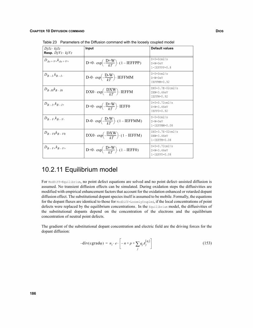
DIOSCHAPTER 10 DIFFUSION COMMAND
10.2.11 Equilibrium model
For ModDiff=Equilibrium, no point defect equations are solved and no point defect–assisted diffusion isassumed. No transient diffusion effects can be simulated. During oxidation steps the diffusivities aremodified with empirical enhancement factors that account for the oxidation enhanced or retarded dopantdiffusion effect. The substitutional dopant species itself is assumed to be mobile. Formally, the equationsfor the dopant fluxes are identical to those for ModDiff=LooselyCoupled, if the local concentrations of pointdefects were replaced by the equilibrium concentrations. In the Equilibrium model, the diffusivities ofthe substitutional dopants depend on the concentration of the electrons and the equilibriumconcentration of neutral point defects.
The gradient of the substitutional dopant concentration and electric field are the driving forces for thedopant diffusion:
(153)
D+0=0cm2/sD+W=0eV1-IEFFPP=0.8
D-0=0cm2/sD-W=0eVIEFFMM=0.92
DX0=3.7E-02cm2/sDXW=3.46eVIEFFM=0.92
D+0=0.72cm2/sD+W=3.46eVIEFF0=0.92
D-0=0cm2/sD-W=0eV1-IEFFMM=0.08
DX0=3.7E-02cm2/sDXW=3.46eV1-IEFFM=0.08
D+0=0.72cm2/sD+W=3.46eV1-IEFF0=0.08
Table 23 Parameters of the Diffusion command with the loosely coupled model
Resp.
Input Default valuesDjIz kjIz⋅DjVz kjVz⋅
DAs V++ kAs V++ D+0 exp⋅ D+WkT
--------------–⎝ ⎠⎛ ⎞ 1 IEFFPP–( )⋅
DB I-– kB I-– D-0 exp⋅ D-WkT
-------------–⎝ ⎠⎛ ⎞ IEFFMM⋅
DB I– 0kB I0– DX0 exp⋅ DXWkT
---------------–⎝ ⎠⎛ ⎞ IEFFM⋅
DB I+– kB I+– D+0 exp⋅ D+WkT
--------------–⎝ ⎠⎛ ⎞ IEFF0⋅
DB V-– kB V-– D-0 exp⋅ D-WkT
-------------–⎝ ⎠⎛ ⎞ 1 IEFFMM–( )⋅
DB V0– kB V0– DX0 exp⋅ DXWkT
---------------–⎝ ⎠⎛ ⎞ 1 IEFFM–( )⋅
DB V+– kB V+– D+0 exp⋅ D+WkT
--------------–⎝ ⎠⎛ ⎞ 1 IEFF0–( )⋅
div εgradϕ( )– ni e n– p qjAjqj[ ]
j∑+ +⋅ ⋅=
186
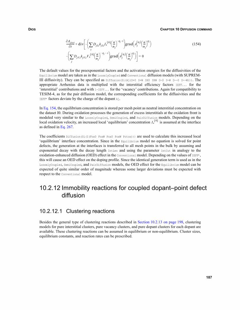
DIOS CHAPTER 10 DIFFUSION COMMAND
(154)
The default values for the preexponential factors and the activation energies for the diffusivities of theEquilibrium model are taken as in the LooselyCoupled and Conventional diffusion models (with SUPREM-III diffusivity). They can be specified as Diffusion(Si(Aj(D+0 D+W DX0 DXW D-0 D-W D--0 D--W))). Theappropriate Arrhenius data is multiplied with the interstitial efficiency factors IEFF... for the‘interstitial’ contributions and with 1-IEFF... for the ‘vacancy’ contributions. Again for compatibility toTESIM-4, as for the pair diffusion model, the corresponding coefficients for the diffusivities and theIEFF* factors deviate by the charge of the dopant Aj.
In Eq. 154, the equilibrium concentration is stored per mesh point as neutral interstitial concentration onthe dataset I0. During oxidation processes the generation of excess interstitials at the oxidation front ismodeled very similar to the LooselyCoupled, SemiCoupled, and PairDiffusion models. Depending on thelocal oxidation velocity, an increased local ‘equilibrium’ concentration is assumed at the interfaceas defined in Eq. 267.
The coefficients Diffusion(Si(I(Fox0 FoxW Pox0 PoxW Potox))) are used to calculate this increased local‘equilibrium’ interface concentration. Since in the Equilibrium model no equation is solved for pointdefects, the generation at the interfaces is transferred to all mesh points in the bulk by assuming andexponential decay with the decay length IntLen and using the parameter IntCut in analogy to theoxidation-enhanced diffusion (OED) effect in the Conventional model. Depending on the values of IEFF*,this will cause an OED effect on the doping profile. Since the identical generation term is used as in theLooselyCoupled, SemiCoupled, and PairDiffusion models, the OED effect for the Equilibrium model can beexpected of quite similar order of magnitude whereas some larger deviations must be expected withrespect to the Conventional model.
10.2.12 Immobility reactions for coupled dopant–point defect diffusion
10.2.12.1 Clustering reactions
Besides the general type of clustering reactions described in Section 10.2.13 on page 198, clusteringmodels for pure interstitial clusters, pure vacancy clusters, and pure dopant clusters for each dopant areavailable. These clustering reactions can be assumed in equilibrium or non-equilibrium. Cluster sizes,equilibrium constants, and reaction rates can be prescribed.
Ajtot∂t∂
-------------- div DjIzkjIzI*0[ ] n
ni----⎝ ⎠
⎛ ⎞qj z––
z∑⎝ ⎠
⎜ ⎟⎛ ⎞
grad Ajqj[ ] n
ni----⎝ ⎠
⎛ ⎞qj
⎝ ⎠⎛ ⎞
DjVzkjVzV*0[ ] n
ni----⎝ ⎠
⎛ ⎞qj– z–
j∑⎝ ⎠
⎜ ⎟⎛ ⎞
grad Ajqj[ ] n
ni----⎝ ⎠
⎛ ⎞qj
⎝ ⎠⎛ ⎞–
–
0=
+
I*0[ ]
187
DIOSCHAPTER 10 DIFFUSION COMMAND
NOTE Although the clustering and diffusion models are selected by the parameters ModDif andModClust, some combinations of these models are not supported. In the ModDif=Conventionalmodel, only ModClust=ZeroElectron | OneElectron | MElectron | Solubility | Table aresupported. In all but the ModDif=Conventional model, ModClust = Solubility |
Table | Transient | Equilibrium | TransientGlobal are supported. Models equivalent toZeroElectron | OneElectron | MElectron can be specified by properly selecting the parametersdefining the composition and the charge of the clusters.
For all clustering models (independent of the diffusion model), additional datasets (ICluster,AsCluster,...) are defined. These datasets define the concentration of clusters. The concentration ofclustered atoms is given by the product of cluster concentration and cluster size. The concentration ofclustered atoms is treated as part of the total concentration of the point defect or the dopant.
To save simulation time, clusters of a particular dopant can be switched off if the maximumconcentration of that dopant is too low. This is accomplished with the parameter TurnOffCluster. Thecriterion for clusters of dopant D to be switched off everywhere in a structure is max(D) <
TurnOffCluster*SolidSolubility(D). (In Release 6.1, this value was fixed at 0.1.) There is a similarparameter DropCluster that acts locally (node by node). Dopant clusters can be switched off locally in thestructure if the concentration is below a certain value.
The criteria is D < DropCluster*SolidSolubility(D). By default, TurnOffCluster=DropCluster.
By default for all but the Transient and TransientGlobal models, the solid solubility is maximized duringthe process, starting with the introduction of the dopant species. The parameterdiff:(MaximizeSolubility=off) can be specified to enforce the solid solubility for the local temperature tobe used.
NOTE This may introduce significant deactivation during a ramp-down.
If the solid solubility has changed due to temperature change, or profiles have diffused away, or all partsof the structure with high doping concentration have been etched away or oxidized and no part of thematerial has high concentration any more, clustering will be switched off globally.
For the Equilibrium, ZeroElectron, OneElectron, and MElectron clustering, an additional nonlinear algebraicequation is solved locally per mesh point. For the Solubility and Table models, a simple cut-off is usedto calculate the active concentrations as a function of the total concentrations. For the non-equilibriumclustering, an ordinary differential equation (o.d.e.) with respect to time is solved. ForModClust=Transient, this o.d.e. is solved with the algebraic equations per mesh point. ForModClust=TransientGlobal, this o.d.e. is solved in the ‘global’ Newton together with the reaction-diffusionequations, thus adding an unknown (and several matrix blocks) to the global Newton solver. Since thedopant in the clusters is treated as part of the total concentration, the clustering reaction terms appearonly in the o.d.e. and they cancel out in the p.d.e. for the total concentration. The clustering model canbe selected for each point defect and dopant. At least for ModClust=TransientGlobal, the same model isassumed in silicon and polysilicon. It is selected by the value of ModClust for silicon. The clustering ratesand equilibrium constants for silicon are used also for the other materials.
188
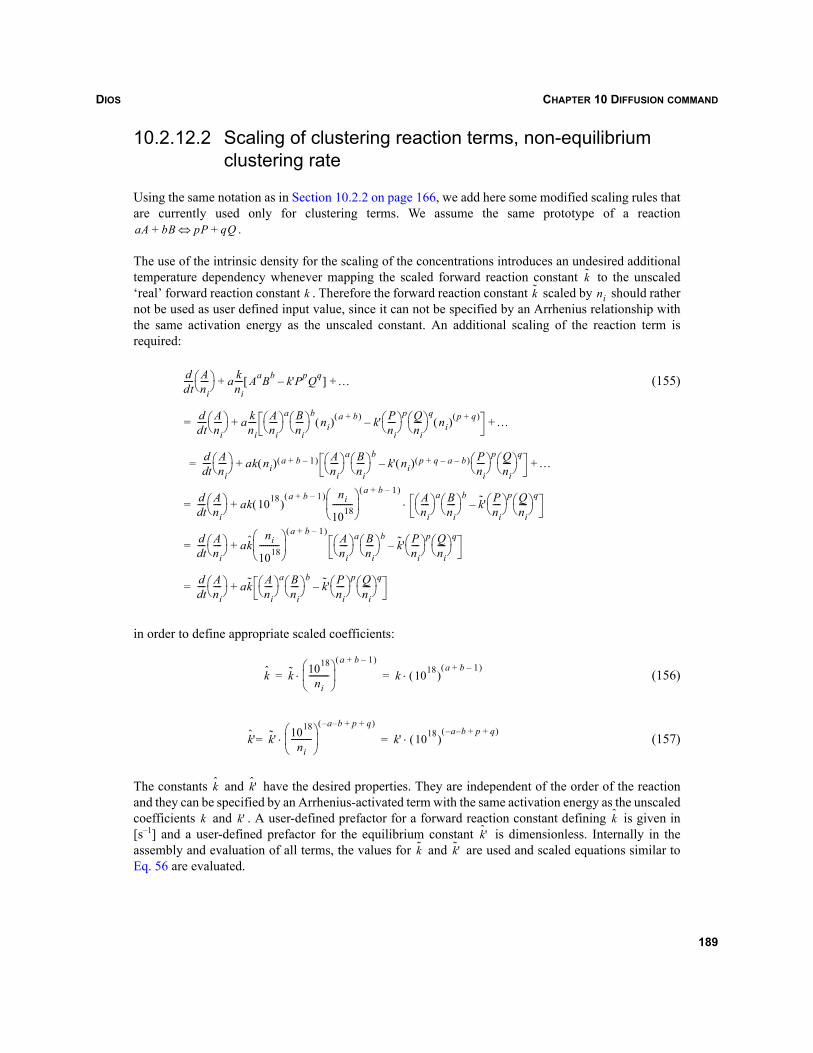
DIOS CHAPTER 10 DIFFUSION COMMAND
10.2.12.2 Scaling of clustering reaction terms, non-equilibrium clustering rate
Using the same notation as in Section 10.2.2 on page 166, we add here some modified scaling rules thatare currently used only for clustering terms. We assume the same prototype of a reaction
.
The use of the intrinsic density for the scaling of the concentrations introduces an undesired additionaltemperature dependency whenever mapping the scaled forward reaction constant to the unscaled‘real’ forward reaction constant . Therefore the forward reaction constant scaled by should rathernot be used as user defined input value, since it can not be specified by an Arrhenius relationship withthe same activation energy as the unscaled constant. An additional scaling of the reaction term isrequired:
(155)
in order to define appropriate scaled coefficients:
(156)
(157)
The constants and have the desired properties. They are independent of the order of the reactionand they can be specified by an Arrhenius-activated term with the same activation energy as the unscaledcoefficients and . A user-defined prefactor for a forward reaction constant defining is given in[s–1] and a user-defined prefactor for the equilibrium constant is dimensionless. Internally in theassembly and evaluation of all terms, the values for and are used and scaled equations similar toEq. 56 are evaluated.
aA bB pP qQ+⇔+
kk k ni
ddt----- A
ni----⎝ ⎠
⎛ ⎞ a kni---- AaBb k'Pp– Qq[ ] …+ +
ddt-----= A
ni----⎝ ⎠
⎛ ⎞ a kni---- A
ni----⎝ ⎠
⎛ ⎞ a Bni----⎝ ⎠
⎛ ⎞ bni( ) a b+( ) k' P
ni----⎝ ⎠
⎛ ⎞ p– Q
ni----⎝ ⎠
⎛ ⎞ qni( ) p q+( ) …+ +
dtd
---- Ani----⎝ ⎠
⎛ ⎞ ak ni( ) a b 1–+( ) Ani----⎝ ⎠
⎛ ⎞ a Bni----⎝ ⎠
⎛ ⎞ bk' ni( ) p q a– b–+( ) P
ni----⎝ ⎠
⎛ ⎞ p– Q
ni----⎝ ⎠
⎛ ⎞ q…
dtd
---- Ani----⎝ ⎠
⎛ ⎞ ak 1018( )a b 1–+( ) ni
1018----------
⎝ ⎠⎜ ⎟⎛ ⎞ a b 1–+( )
Ani----⎝ ⎠
⎛ ⎞ a Bni----⎝ ⎠
⎛ ⎞ bk'˜ P
ni----⎝ ⎠
⎛ ⎞ p– Q
ni----⎝ ⎠
⎛ ⎞ q
dtd
---- Ani----⎝ ⎠
⎛ ⎞ akni
1018----------
⎝ ⎠⎜ ⎟⎛ ⎞ a b 1–+( )
Ani----⎝ ⎠
⎛ ⎞ a Bni----⎝ ⎠
⎛ ⎞ bk'˜ P
ni----⎝ ⎠
⎛ ⎞ p– Q
ni----⎝ ⎠
⎛ ⎞ q
dtd
---- Ani----⎝ ⎠
⎛ ⎞ ak Ani----⎝ ⎠
⎛ ⎞ a Bni----⎝ ⎠
⎛ ⎞ bk'˜ P
ni----⎝ ⎠
⎛ ⎞ p– Q
ni----⎝ ⎠
⎛ ⎞ q+=
+=
⋅+=
+ +=
k k 1018
ni----------
⎝ ⎠⎜ ⎟⎛ ⎞
a b 1–+( )
⋅ k 1018( )a b 1–+( )
⋅= =
k'ˆ k'˜ 1018
ni----------
⎝ ⎠⎜ ⎟⎛ ⎞
a– b– p q+ +( )
⋅= k' 1018( )a– b– p q+ +( )
⋅=
k k'ˆ
k k' kk'ˆ
k k'˜
189
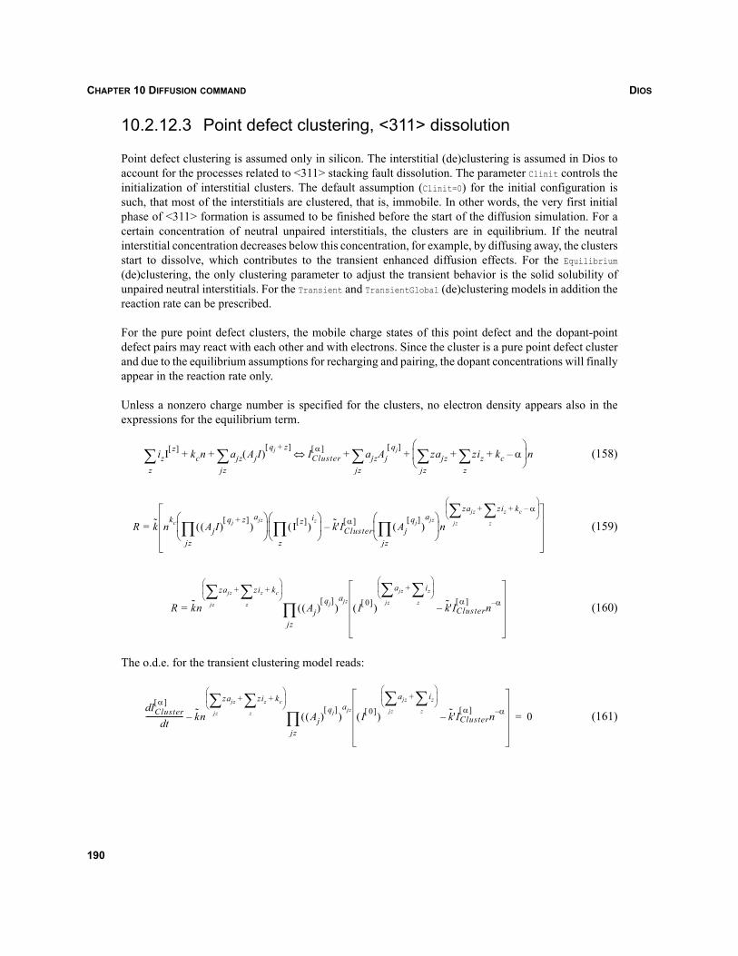
DIOSCHAPTER 10 DIFFUSION COMMAND
10.2.12.3 Point defect clustering, <311> dissolution
Point defect clustering is assumed only in silicon. The interstitial (de)clustering is assumed in Dios toaccount for the processes related to <311> stacking fault dissolution. The parameter Clinit controls theinitialization of interstitial clusters. The default assumption (Clinit=0) for the initial configuration issuch, that most of the interstitials are clustered, that is, immobile. In other words, the very first initialphase of <311> formation is assumed to be finished before the start of the diffusion simulation. For acertain concentration of neutral unpaired interstitials, the clusters are in equilibrium. If the neutralinterstitial concentration decreases below this concentration, for example, by diffusing away, the clustersstart to dissolve, which contributes to the transient enhanced diffusion effects. For the Equilibrium(de)clustering, the only clustering parameter to adjust the transient behavior is the solid solubility ofunpaired neutral interstitials. For the Transient and TransientGlobal (de)clustering models in addition thereaction rate can be prescribed.
For the pure point defect clusters, the mobile charge states of this point defect and the dopant-pointdefect pairs may react with each other and with electrons. Since the cluster is a pure point defect clusterand due to the equilibrium assumptions for recharging and pairing, the dopant concentrations will finallyappear in the reaction rate only.
Unless a nonzero charge number is specified for the clusters, no electron density appears also in theexpressions for the equilibrium term.
(158)
(159)
(160)
The o.d.e. for the transient clustering model reads:
(161)
izIz[ ]
z∑ kcn ajz AjI( )
qj z+[ ]ICluster
α[ ] ajzAjqj[ ]
zajz ziz kc α–+z
∑+jz∑⎝ ⎠
⎜ ⎟⎛ ⎞
n+jz∑+⇔
jz∑+ +
R k= nkc AjI( )
qj z+[ ]( )
ajz
jz∏⎝ ⎠
⎜ ⎟⎛ ⎞
I z[ ]( )iz
z∏⎝ ⎠
⎜ ⎟⎛ ⎞
k'˜ IClusterα[ ] Aj
qj[ ]( )
ajz
jz∏⎝ ⎠
⎜ ⎟⎛ ⎞
n
zajz ziz kc α–+
z∑+
jz∑⎝ ⎠
⎜ ⎟⎛ ⎞
–
R k= n
zajz ziz kc+
z∑+
jz∑⎝ ⎠
⎜ ⎟⎛ ⎞
Aj( )qj[ ]
( )ajz
I 0[ ]( )
ajz iz
z∑+
jz∑⎝ ⎠
⎜ ⎟⎛ ⎞
k'˜ IClusterα[ ]
n α––jz∏
Id Clusterα[ ]
td--------------------- k– n
zajz ziz kc+
z∑+
jz∑⎝ ⎠
⎜ ⎟⎛ ⎞
Aj( )qj[ ]
( )ajz
I 0[ ]( )
ajz iz
z∑+
jz∑⎝ ⎠
⎜ ⎟⎛ ⎞
k'˜ IClusterα[ ]
n α––jz∏ 0=
190
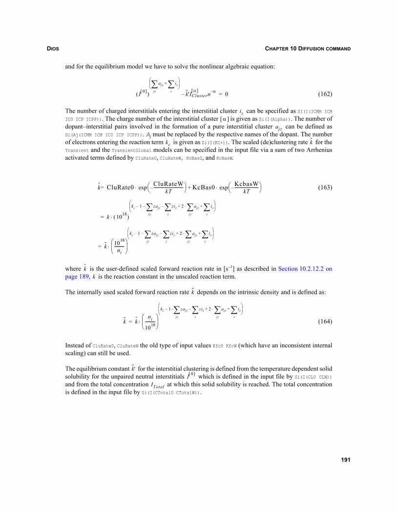
DIOS CHAPTER 10 DIFFUSION COMMAND
and for the equilibrium model we have to solve the nonlinear algebraic equation:
(162)
The number of charged interstitials entering the interstitial cluster can be specified as SI(I(ICMM ICMIC0 ICP ICPP)). The charge number of the interstitial cluster is given as Si(I(Alpha)). The number ofdopant–interstitial pairs involved in the formation of a pure interstitial cluster can be defined asSi(Aj(ICMM ICM IC0 ICP ICPP)). Aj must be replaced by the respective names of the dopant. The numberof electrons entering the reaction term is given as Si(I(KC+)). The scaled (de)clustering rate for theTransient and the TransientGlobal models can be specified in the input file via a sum of two Arrheniusactivated terms defined by CluRate0, CluRateW, KcBas0, and KcBasW.
(163)
where is the user-defined scaled forward reaction rate in [s–1] as described in Section 10.2.12.2 onpage 189, is the reaction constant in the unscaled reaction term.
The internally used scaled forward reaction rate depends on the intrinsic density and is defined as:
(164)
Instead of CluRate0, CluRateW the old type of input values Kfc0 KfcW (which have an inconsistent internalscaling) can still be used.
The equilibrium constant for the interstitial clustering is defined from the temperature dependent solidsolubility for the unpaired neutral interstitials which is defined in the input file by Si(I(CL0 CLW))and from the total concentration at which this solid solubility is reached. The total concentrationis defined in the input file by Si(I(CTotal0 CTotalW)).
I 0[ ]( )
ajz iz
z∑+
jz∑⎝ ⎠
⎜ ⎟⎛ ⎞
k'˜ IClusterα[ ]
n α–– 0=
izα[ ]
ajz
kc k
k CluRate0 CluRateWkT
------------------------------–⎝ ⎠⎛ ⎞exp KcBas0 KcbasW
kT------------------------–⎝ ⎠
⎛ ⎞exp⋅+⋅=
k 1018( )
kc 1– zajz ziz 2 ajz iz
z∑+
jz∑⋅+
z∑–
jz∑–
⎝ ⎠⎜ ⎟⎛ ⎞
k 1018
ni----------
⎝ ⎠⎜ ⎟⎛ ⎞
kc 1– zajz ziz 2 ajz iz
z∑+
jz∑⋅+
z∑–
jz∑–
⎝ ⎠⎜ ⎟⎛ ⎞
⋅=
⋅=
kk
k
k kni
1018----------
⎝ ⎠⎜ ⎟⎛ ⎞
kc 1 zajz ziz 2 ajz iz
z∑+
jz∑⋅+
z∑–
jz∑––
⎝ ⎠⎜ ⎟⎛ ⎞
⋅=
k'˜
I 0[ ]
ITotal
191
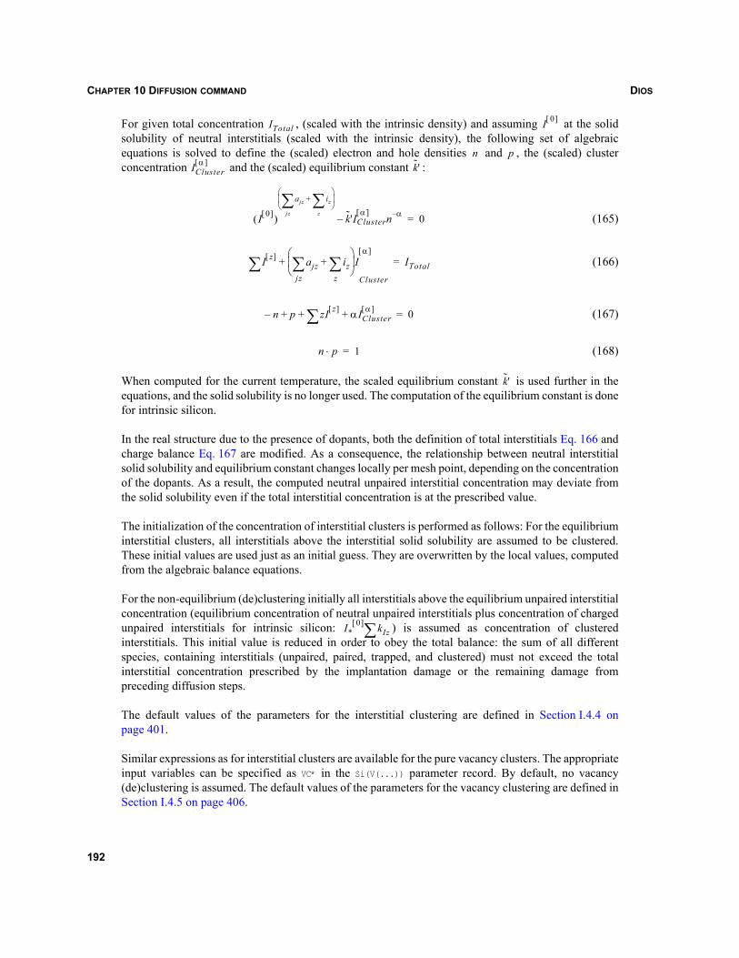
DIOSCHAPTER 10 DIFFUSION COMMAND
For given total concentration , (scaled with the intrinsic density) and assuming at the solidsolubility of neutral interstitials (scaled with the intrinsic density), the following set of algebraicequations is solved to define the (scaled) electron and hole densities and , the (scaled) clusterconcentration and the (scaled) equilibrium constant :
(165)
(166)
(167)
(168)
When computed for the current temperature, the scaled equilibrium constant is used further in theequations, and the solid solubility is no longer used. The computation of the equilibrium constant is donefor intrinsic silicon.
In the real structure due to the presence of dopants, both the definition of total interstitials Eq. 166 andcharge balance Eq. 167 are modified. As a consequence, the relationship between neutral interstitialsolid solubility and equilibrium constant changes locally per mesh point, depending on the concentrationof the dopants. As a result, the computed neutral unpaired interstitial concentration may deviate fromthe solid solubility even if the total interstitial concentration is at the prescribed value.
The initialization of the concentration of interstitial clusters is performed as follows: For the equilibriuminterstitial clusters, all interstitials above the interstitial solid solubility are assumed to be clustered.These initial values are used just as an initial guess. They are overwritten by the local values, computedfrom the algebraic balance equations.
For the non-equilibrium (de)clustering initially all interstitials above the equilibrium unpaired interstitialconcentration (equilibrium concentration of neutral unpaired interstitials plus concentration of chargedunpaired interstitials for intrinsic silicon: ) is assumed as concentration of clusteredinterstitials. This initial value is reduced in order to obey the total balance: the sum of all differentspecies, containing interstitials (unpaired, paired, trapped, and clustered) must not exceed the totalinterstitial concentration prescribed by the implantation damage or the remaining damage frompreceding diffusion steps.
The default values of the parameters for the interstitial clustering are defined in Section I.4.4 onpage 401.
Similar expressions as for interstitial clusters are available for the pure vacancy clusters. The appropriateinput variables can be specified as VC* in the Si(V(...)) parameter record. By default, no vacancy(de)clustering is assumed. The default values of the parameters for the vacancy clustering are defined inSection I.4.5 on page 406.
ITotal I 0[ ]
n pICluster
α[ ] k'˜
I 0[ ]( )
ajz iz
z∑+
jz∑⎝ ⎠
⎜ ⎟⎛ ⎞
k'˜ IClusterα[ ]
n α–– 0=
I z[ ]∑ ajz iz
z∑+
jz∑⎝ ⎠
⎜ ⎟⎛ ⎞
ICluster
α[ ]+ ITotal=
n p zI z[ ]∑+ +– αICluster
α[ ]+ 0=
n p⋅ 1=
k'˜
I*0[ ] kIz∑
192
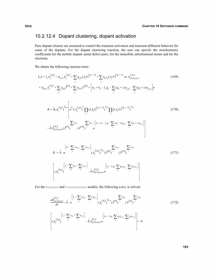
DIOS CHAPTER 10 DIFFUSION COMMAND
10.2.12.4 Dopant clustering, dopant activation
Pure dopant clusters are assumed to control the transient activation and transient diffusion behavior forsome of the dopants. For the dopant clustering reaction, the user can specify the stoichiometrycoefficients for the mobile dopant–point defect pairs, for the immobile substitutional atoms and for theelectrons.
We obtain the following reaction term:
(169)
(170)
(171)
For the Transient and TransientGlobal models, the following o.d.e. is solved:
(172)
kcn lcAjqj[ ]
+ dencAjqj[ ]
ajIz AjI( )qj z+[ ]
z∑ ajVz AjV( )
qj z+[ ]AjCluster
αj[ ]
dencAjqj[ ]
ajIzI0[ ]
z∑ ajVzV
0[ ] αj kc lcqj qj z+( )ajIz qj z+( )ajVzz
∑–z
∑––+⎝ ⎠⎜ ⎟⎛ ⎞
n+z
∑+ + +
⇔z
∑+ + +
R k Ajqj[ ]
( )denc
= nkc Aj
qj[ ]( )
lcAjI( )
qj z+[ ]( )
z∏
ajIzAjV( )
qj z+[ ]( )
z∏
ajVz
k'˜ AjClusterαj[ ]
I 0[ ]( )
ajIz
z∑
V 0[ ]( )
ajVz
z∑
n
αj kc lcqj qj z+( )ajIz qj z+( )ajVz
z∑–
z∑––+
⎝ ⎠⎜ ⎟⎛ ⎞
–
R k n⋅
kc zajIz zajVz
z∑–
jz∑–
⎝ ⎠⎜ ⎟⎛ ⎞
Ajqj[ ]
( )denc
I 0[ ]( )
ajIz
z∑
V 0[ ]( )
ajVz
z∑
Ajqj[ ]
( )
lc ajIz ajVz
z∑+
jz∑+
⎝ ⎠⎜ ⎟⎛ ⎞
k'˜ AjClusterαj[ ]
n
αj lcqj qjajIz qjajVz
z∑–
jz∑––
⎝ ⎠⎜ ⎟⎛ ⎞
–
=
AjClusterαj[ ]
ddt
------------------------ k n⋅
kc zajIz zajVz
z∑–
jz∑–
⎝ ⎠⎜ ⎟⎛ ⎞
– Ajqj[ ]
( )denc
I 0[ ]( )
ajIz
z∑
V 0[ ]( )
ajVz
z∑
Ajqj[ ]
( )
lc ajIz ajVz
z∑+
jz∑+
⎝ ⎠⎜ ⎟⎛ ⎞
k'˜ AjClusterαj[ ]
n
αj lcqj qjajIz qjajVz
z∑–
jz∑––
⎝ ⎠⎜ ⎟⎛ ⎞
– 0=
193
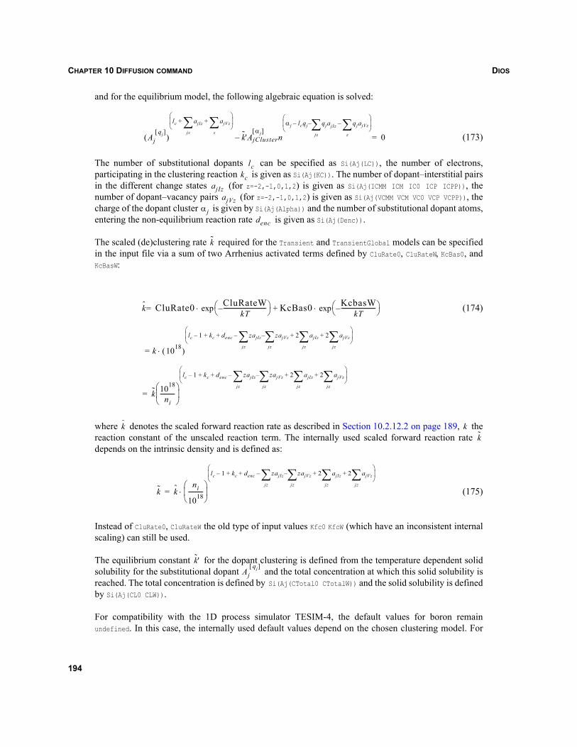
DIOSCHAPTER 10 DIFFUSION COMMAND
and for the equilibrium model, the following algebraic equation is solved:
(173)
The number of substitutional dopants can be specified as Si(Aj(LC)), the number of electrons,participating in the clustering reaction is given as Si(Aj(KC)). The number of dopant–interstitial pairsin the different change states (for z=-2,-1,0,1,2) is given as Si(Aj(ICMM ICM IC0 ICP ICPP)), thenumber of dopant–vacancy pairs (for z=-2,-1,0,1,2) is given as Si(Aj(VCMM VCM VC0 VCP VCPP)), thecharge of the dopant cluster is given by Si(Aj(Alpha)) and the number of substitutional dopant atoms,entering the non-equilibrium reaction rate is given as Si(Aj(Denc)).
The scaled (de)clustering rate required for the Transient and TransientGlobal models can be specifiedin the input file via a sum of two Arrhenius activated terms defined by CluRate0, CluRateW, KcBas0, andKcBasW:
(174)
where denotes the scaled forward reaction rate as described in Section 10.2.12.2 on page 189, thereaction constant of the unscaled reaction term. The internally used scaled forward reaction rate depends on the intrinsic density and is defined as:
(175)
Instead of CluRate0, CluRateW the old type of input values Kfc0 KfcW (which have an inconsistent internalscaling) can still be used.
The equilibrium constant for the dopant clustering is defined from the temperature dependent solidsolubility for the substitutional dopant and the total concentration at which this solid solubility isreached. The total concentration is defined by Si(Aj(CTotal0 CTotalW)) and the solid solubility is definedby Si(Aj(CL0 CLW)).
For compatibility with the 1D process simulator TESIM-4, the default values for boron remainundefined. In this case, the internally used default values depend on the chosen clustering model. For
Ajqj[ ]
( )
lc ajIz ajVz
z∑+
jz∑+
⎝ ⎠⎜ ⎟⎛ ⎞
k'˜ AjClusterαj[ ]
n
αj lcqj qjajIz qjajVz
z∑–
jz∑––
⎝ ⎠⎜ ⎟⎛ ⎞
– 0=
lckc
ajIzajVz
αjdenc
k
k CluRate0 CluRateWkT
------------------------------–⎝ ⎠⎛ ⎞ KcBas0 KcbasW
kT------------------------–⎝ ⎠
⎛ ⎞exp⋅+exp⋅=
k 1018( )
lc 1– kc denc zajIz zajVz 2 ajIz
jz∑+
jz∑– 2 ajVz
jz∑+
jz∑–+ +
⎝ ⎠⎜ ⎟⎛ ⎞
⋅=
k 1018
ni----------
⎝ ⎠⎜ ⎟⎛ ⎞
lc 1– kc denc zajIz zajVz 2 ajIz
jz∑+
jz∑– 2 ajVz
jz∑+
jz∑–+ +
⎝ ⎠⎜ ⎟⎛ ⎞
=
k kk
k kni
1018----------
⎝ ⎠⎜ ⎟⎛ ⎞
lc 1– kc denc zajIz zajVz 2 ajIz
jz∑+
jz∑– 2 ajVz
jz∑+
jz∑–+ +
⎝ ⎠⎜ ⎟⎛ ⎞
⋅=
k'˜
Ajqj[ ]
194
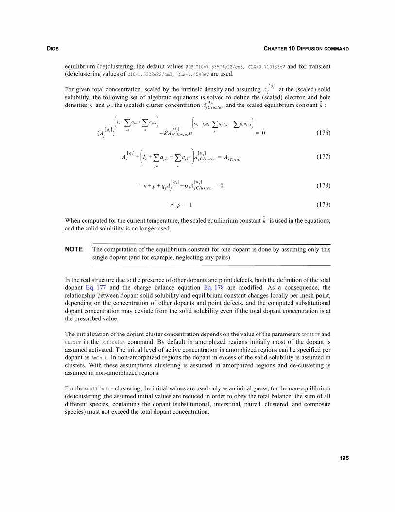
DIOS CHAPTER 10 DIFFUSION COMMAND
equilibrium (de)clustering, the default values are Cl0=7.53573e22/cm3, CLW=0.710133eV and for transient(de)clustering values of Cl0=1.5322e22/cm3, CLW=0.4593eV are used.
For given total concentration, scaled by the intrinsic density and assuming at the (scaled) solidsolubility, the following set of algebraic equations is solved to define the (scaled) electron and holedensities and , the (scaled) cluster concentration and the scaled equilibrium constant :
(176)
(177)
(178)
(179)
When computed for the current temperature, the scaled equilibrium constant is used in the equations,and the solid solubility is no longer used.
NOTE The computation of the equilibrium constant for one dopant is done by assuming only thissingle dopant (and for example, neglecting any pairs).
In the real structure due to the presence of other dopants and point defects, both the definition of the totaldopant Eq. 177 and the charge balance equation Eq. 178 are modified. As a consequence, therelationship between dopant solid solubility and equilibrium constant changes locally per mesh point,depending on the concentration of other dopants and point defects, and the computed substitutionaldopant concentration may deviate from the solid solubility even if the total dopant concentration is atthe prescribed value.
The initialization of the dopant cluster concentration depends on the value of the parameters DOPINIT andCLINIT in the Diffusion command. By default in amorphized regions initially most of the dopant isassumed activated. The initial level of active concentration in amorphized regions can be specified perdopant as AmInit. In non-amorphized regions the dopant in excess of the solid solubility is assumed inclusters. With these assumptions clustering is assumed in amorphized regions and de-clustering isassumed in non-amorphized regions.
For the Equilibrium clustering, the initial values are used only as an initial guess, for the non-equilibrium(de)clustering ,the assumed initial values are reduced in order to obey the total balance: the sum of alldifferent species, containing the dopant (substitutional, interstitial, paired, clustered, and compositespecies) must not exceed the total dopant concentration.
Ajqj[ ]
n p AjClusterαj[ ]
k'˜
Ajqj[ ]
( )
lc ajIz ajVz
z∑+
jz∑+
⎝ ⎠⎜ ⎟⎛ ⎞
k'˜ AjClusterαj[ ]
n
αj lcqj qjajIz qjajVz
z∑–
jz∑––
⎝ ⎠⎜ ⎟⎛ ⎞
– 0=
Ajqj[ ]
lc ajIz ajVzz
∑+jz∑+
⎝ ⎠⎜ ⎟⎛ ⎞
AjClusterαj[ ]
+ AjTotal=
n p qjAjqj[ ]
+ +– αjAjClusterαj[ ]
+ 0=
n p⋅ 1=
k'˜
195
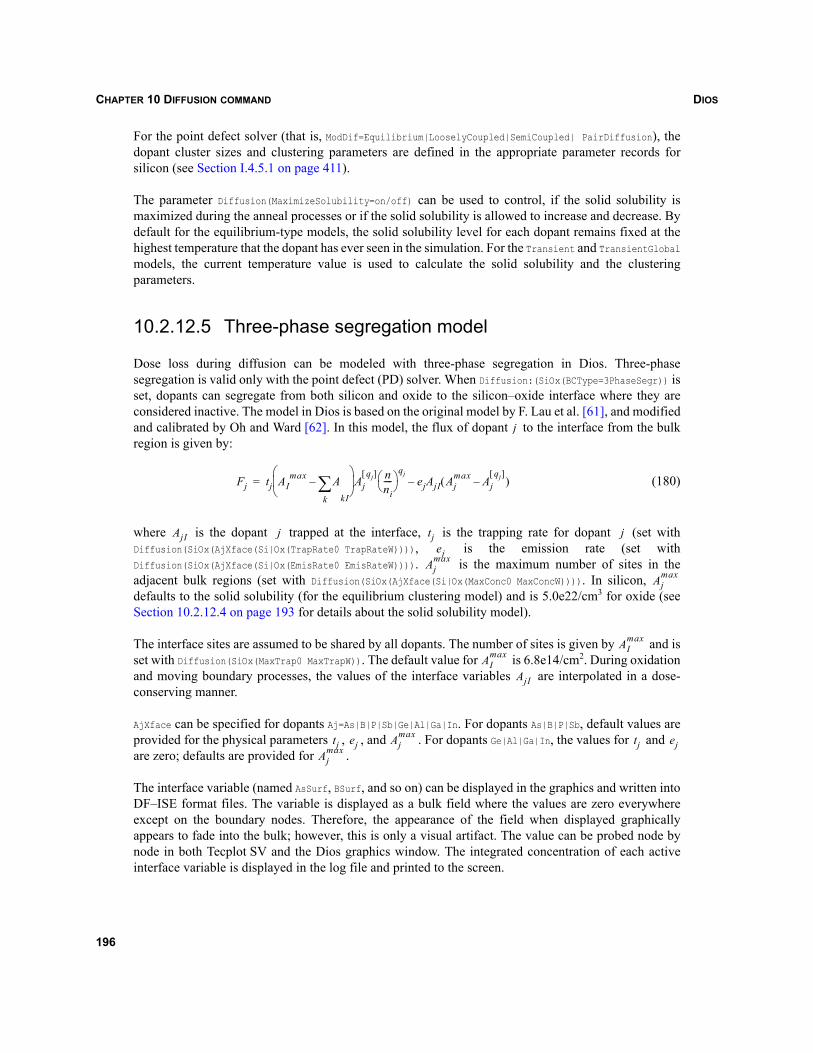
DIOSCHAPTER 10 DIFFUSION COMMAND
For the point defect solver (that is, ModDif=Equilibrium|LooselyCoupled|SemiCoupled| PairDiffusion), thedopant cluster sizes and clustering parameters are defined in the appropriate parameter records forsilicon (see Section I.4.5.1 on page 411).
The parameter Diffusion(MaximizeSolubility=on/off) can be used to control, if the solid solubility ismaximized during the anneal processes or if the solid solubility is allowed to increase and decrease. Bydefault for the equilibrium-type models, the solid solubility level for each dopant remains fixed at thehighest temperature that the dopant has ever seen in the simulation. For the Transient and TransientGlobalmodels, the current temperature value is used to calculate the solid solubility and the clusteringparameters.
10.2.12.5 Three-phase segregation model
Dose loss during diffusion can be modeled with three-phase segregation in Dios. Three-phasesegregation is valid only with the point defect (PD) solver. When Diffusion:(SiOx(BCType=3PhaseSegr)) isset, dopants can segregate from both silicon and oxide to the silicon–oxide interface where they areconsidered inactive. The model in Dios is based on the original model by F. Lau et al. [61], and modifiedand calibrated by Oh and Ward [62]. In this model, the flux of dopant to the interface from the bulkregion is given by:
(180)
where is the dopant trapped at the interface, is the trapping rate for dopant (set withDiffusion(SiOx(AjXface(Si|Ox(TrapRate0 TrapRateW)))), is the emission rate (set withDiffusion(SiOx(AjXface(Si|Ox(EmisRate0 EmisRateW)))). is the maximum number of sites in theadjacent bulk regions (set with Diffusion(SiOx(AjXface(Si|Ox(MaxConc0 MaxConcW)))). In silicon, defaults to the solid solubility (for the equilibrium clustering model) and is 5.0e22/cm3 for oxide (seeSection 10.2.12.4 on page 193 for details about the solid solubility model).
The interface sites are assumed to be shared by all dopants. The number of sites is given by and isset with Diffusion(SiOx(MaxTrap0 MaxTrapW)). The default value for is 6.8e14/cm2. During oxidationand moving boundary processes, the values of the interface variables are interpolated in a dose-conserving manner.
AjXface can be specified for dopants Aj=As|B|P|Sb|Ge|Al|Ga|In. For dopants As|B|P|Sb, default values areprovided for the physical parameters , , and . For dopants Ge|Al|Ga|In, the values for and are zero; defaults are provided for .
The interface variable (named AsSurf, BSurf, and so on) can be displayed in the graphics and written intoDF–ISE format files. The variable is displayed as a bulk field where the values are zero everywhereexcept on the boundary nodes. Therefore, the appearance of the field when displayed graphicallyappears to fade into the bulk; however, this is only a visual artifact. The value can be probed node bynode in both Tecplot SV and the Dios graphics window. The integrated concentration of each activeinterface variable is displayed in the log file and printed to the screen.
j
Fj tj AImax A
k∑
kI
–⎝ ⎠⎜ ⎟⎛ ⎞
Ajqj[ ] n
ni----⎝ ⎠
⎛ ⎞qj
ejAjI Ajmax Aj
qj[ ]–( )–=
AjI j tj jej
Ajmax
Ajmax
AImax
AImax
AjI
tj ej Ajmax tj ej
Ajmax
196
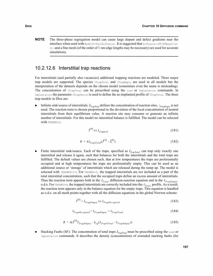
DIOS CHAPTER 10 DIFFUSION COMMAND
NOTE The three-phase segregation model can cause large dopant and defect gradients near theinterface when used with ModDiff=PairDiffusion. It is suggested that Diffusion:(DT(DTBegin=1e-6)) and a fine mesh (of the order of 1 nm edge lengths may be necessary) are used for accuratesimulations.
10.2.12.6 Interstitial trap reactions
For interstitials (and partially also vacancies) additional trapping reactions are modeled. Three majortrap models are supported. The species ITrapTotal and ITrapEmpty are used in all models but theinterpretation of the datasets depends on the chosen model (sometimes even the name is misleading).The concentration of ITrapTotal can be prescribed using the Load or Implantation commands. InImplantation the parameter ITrapFactor is used to define the as-implanted profile of ITrapTotal. The threetrap models in Dios are:
Infinite sink/source of interstitials: ITrapTotal defines the concentration of reaction sites, ITrapEmpty is notused. The reaction term is chosen proportional to the deviation of the local concentration of neutralinterstitials from their equilibrium value. A reaction site may consume or generate an infinitenumber of interstitials. For this model no interstitial balance is fulfilled. The model can be selectedwith TRAPMOD=2.
(181)
(182)
Finite interstitial sink/source. Each of the traps, specified as ITrapTotal, can trap only exactly oneinterstitial and release it again, such that balances for both the interstitials and the total traps arefulfilled. The default values are chosen such, that at low temperatures the traps are preferentiallyoccupied and at high temperatures the traps are preferentially empty. This can be used as anadditional source or ‘storage’ of interstitials which are released during the ramp up. The model isselected with TRAPMOD=3|4. For TRAPMOD=3, the trapped interstitials are not included as a part of thetotal interstitial concentration, such that the occupied traps define an excess amount of interstitials.Thus the reaction term appears both in the diffusion-reaction equation and in the o.d.e. For TRAPMOD=4, the trapped interstitials are correctly included into the profile. As a result,the reaction term appears only in the balance equation for the empty traps. This equation is handledas o.d.e. on all mesh points together with all the diffusion equations in the global Newton scheme:
(183)
(184)
(185)
Stacking Faults (SF): The concentration of total traps ITrapTotal must be prescribed using the Load orImplantation commands. It describes the density (concentration) of extended stacking faults (for
I 0[ ] Itrapped⇔
R kITrapTotal I 0[ ] I*0[ ]–( )=
ITotal ITrapEmptyITotal
I 0[ ] ITrapEmpty+ ITrapOccupied⇔
ITrapOccupied ITrapEmpty ITrapTotal=+
R k I 0[ ]ITrapEmpty keq ITrapTtotal ITrapEmpty–( )–( )=
197
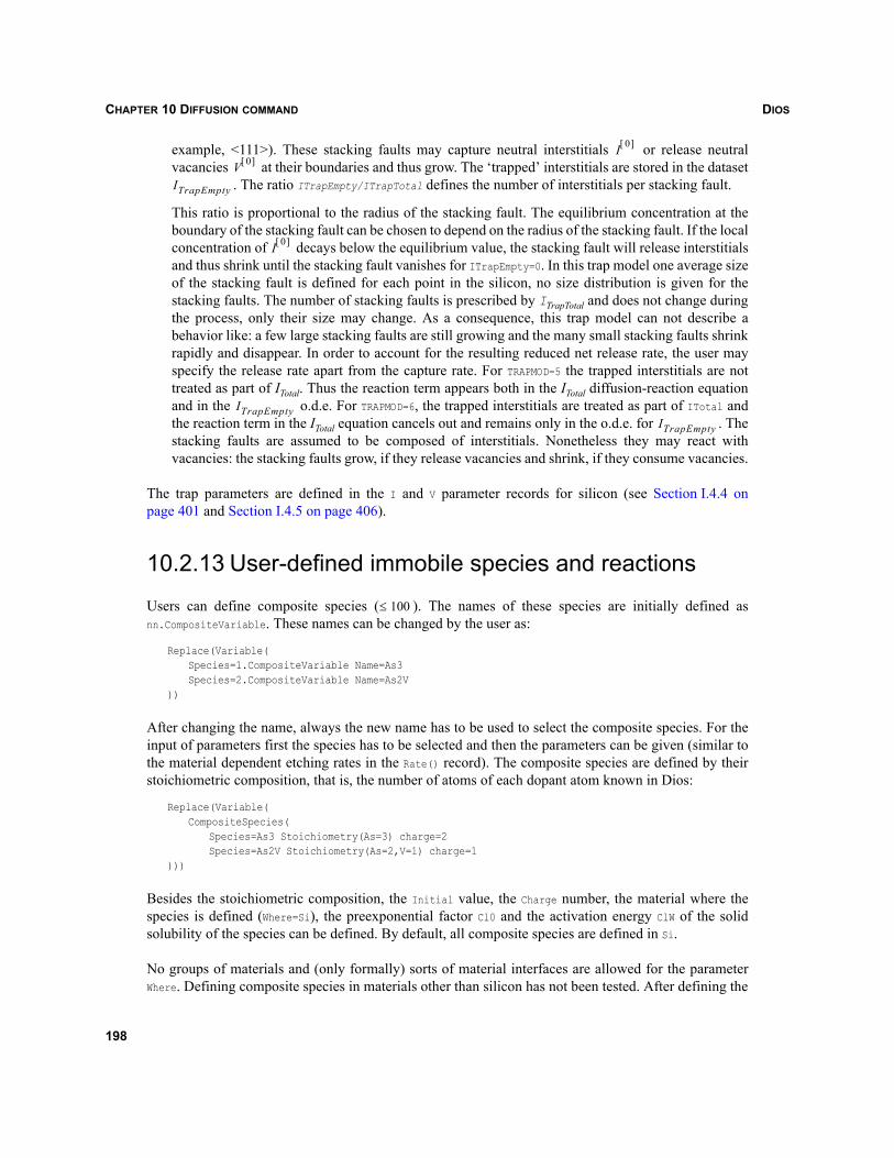
DIOSCHAPTER 10 DIFFUSION COMMAND
example, <111>). These stacking faults may capture neutral interstitials or release neutralvacancies at their boundaries and thus grow. The ‘trapped’ interstitials are stored in the dataset
. The ratio ITrapEmpty/ITrapTotal defines the number of interstitials per stacking fault.
This ratio is proportional to the radius of the stacking fault. The equilibrium concentration at theboundary of the stacking fault can be chosen to depend on the radius of the stacking fault. If the localconcentration of decays below the equilibrium value, the stacking fault will release interstitialsand thus shrink until the stacking fault vanishes for ITrapEmpty=0. In this trap model one average sizeof the stacking fault is defined for each point in the silicon, no size distribution is given for thestacking faults. The number of stacking faults is prescribed by ITrapTotal and does not change duringthe process, only their size may change. As a consequence, this trap model can not describe abehavior like: a few large stacking faults are still growing and the many small stacking faults shrinkrapidly and disappear. In order to account for the resulting reduced net release rate, the user mayspecify the release rate apart from the capture rate. For TRAPMOD=5 the trapped interstitials are nottreated as part of ITotal. Thus the reaction term appears both in the ITotal diffusion-reaction equationand in the o.d.e. For TRAPMOD=6, the trapped interstitials are treated as part of ITotal andthe reaction term in the ITotal equation cancels out and remains only in the o.d.e. for . Thestacking faults are assumed to be composed of interstitials. Nonetheless they may react withvacancies: the stacking faults grow, if they release vacancies and shrink, if they consume vacancies.
The trap parameters are defined in the I and V parameter records for silicon (see Section I.4.4 onpage 401 and Section I.4.5 on page 406).
10.2.13 User-defined immobile species and reactions
Users can define composite species ( ). The names of these species are initially defined asnn.CompositeVariable. These names can be changed by the user as:
Replace(Variable(Species=1.CompositeVariable Name=As3Species=2.CompositeVariable Name=As2V
))
After changing the name, always the new name has to be used to select the composite species. For theinput of parameters first the species has to be selected and then the parameters can be given (similar tothe material dependent etching rates in the Rate() record). The composite species are defined by theirstoichiometric composition, that is, the number of atoms of each dopant atom known in Dios:
Replace(Variable(CompositeSpecies(
Species=As3 Stoichiometry(As=3) charge=2Species=As2V Stoichiometry(As=2,V=1) charge=1
)))
Besides the stoichiometric composition, the Initial value, the Charge number, the material where thespecies is defined (Where=Si), the preexponential factor Cl0 and the activation energy ClW of the solidsolubility of the species can be defined. By default, all composite species are defined in Si.
No groups of materials and (only formally) sorts of material interfaces are allowed for the parameterWhere. Defining composite species in materials other than silicon has not been tested. After defining the
I 0[ ]
V 0[ ]
ITrapEmpty
I 0[ ]
ITrapEmptyITrapEmpty
100≤
198
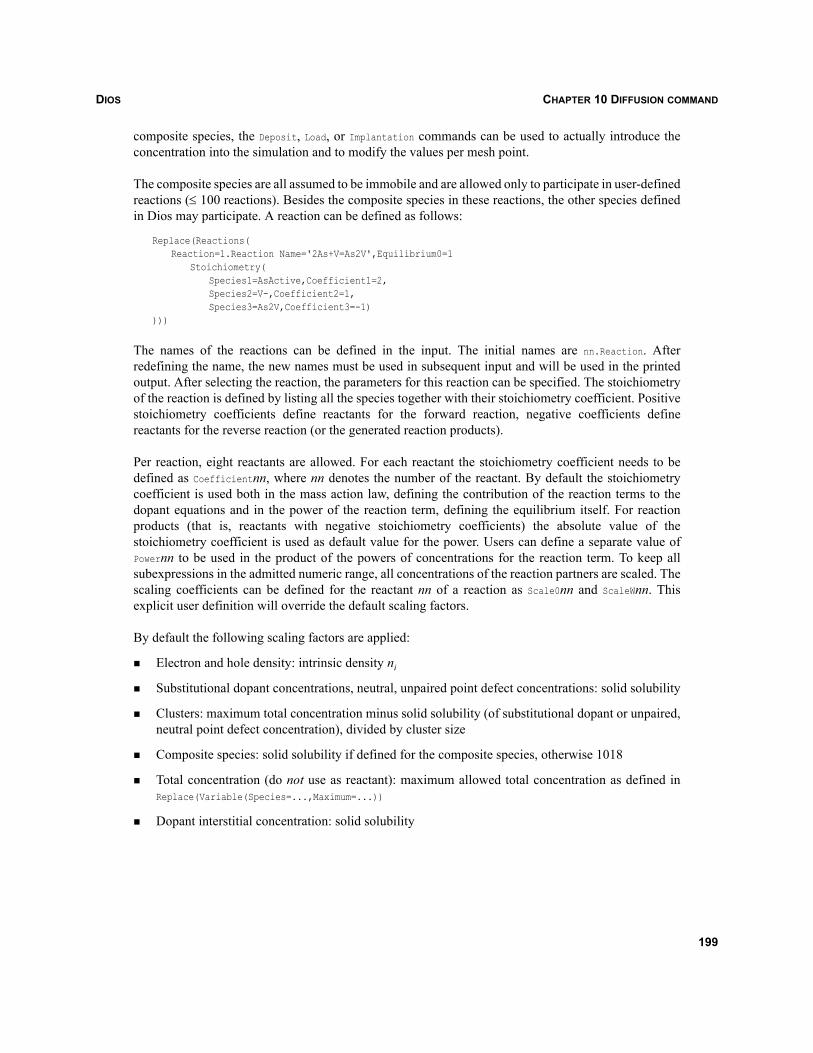
DIOS CHAPTER 10 DIFFUSION COMMAND
composite species, the Deposit, Load, or Implantation commands can be used to actually introduce theconcentration into the simulation and to modify the values per mesh point.
The composite species are all assumed to be immobile and are allowed only to participate in user-definedreactions (≤ 100 reactions). Besides the composite species in these reactions, the other species definedin Dios may participate. A reaction can be defined as follows:
Replace(Reactions(Reaction=1.Reaction Name='2As+V=As2V',Equilibrium0=1
Stoichiometry(Species1=AsActive,Coefficient1=2,Species2=V-,Coefficient2=1,Species3=As2V,Coefficient3=-1)
)))
The names of the reactions can be defined in the input. The initial names are nn.Reaction. Afterredefining the name, the new names must be used in subsequent input and will be used in the printedoutput. After selecting the reaction, the parameters for this reaction can be specified. The stoichiometryof the reaction is defined by listing all the species together with their stoichiometry coefficient. Positivestoichiometry coefficients define reactants for the forward reaction, negative coefficients definereactants for the reverse reaction (or the generated reaction products).
Per reaction, eight reactants are allowed. For each reactant the stoichiometry coefficient needs to bedefined as Coefficientnn, where nn denotes the number of the reactant. By default the stoichiometrycoefficient is used both in the mass action law, defining the contribution of the reaction terms to thedopant equations and in the power of the reaction term, defining the equilibrium itself. For reactionproducts (that is, reactants with negative stoichiometry coefficients) the absolute value of thestoichiometry coefficient is used as default value for the power. Users can define a separate value ofPowernn to be used in the product of the powers of concentrations for the reaction term. To keep allsubexpressions in the admitted numeric range, all concentrations of the reaction partners are scaled. Thescaling coefficients can be defined for the reactant nn of a reaction as Scale0nn and ScaleWnn. Thisexplicit user definition will override the default scaling factors.
By default the following scaling factors are applied:
Electron and hole density: intrinsic density ni
Substitutional dopant concentrations, neutral, unpaired point defect concentrations: solid solubility
Clusters: maximum total concentration minus solid solubility (of substitutional dopant or unpaired,neutral point defect concentration), divided by cluster size
Composite species: solid solubility if defined for the composite species, otherwise 1018
Total concentration (do not use as reactant): maximum allowed total concentration as defined inReplace(Variable(Species=...,Maximum=...))
Dopant interstitial concentration: solid solubility
199
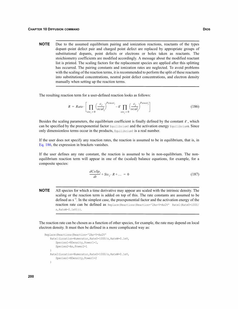
DIOSCHAPTER 10 DIFFUSION COMMAND
NOTE Due to the assumed equilibrium pairing and ionization reactions, reactants of the typesdopant–point defect pair and charged point defect are replaced by appropriate groups ofsubstitutional dopants, point defects or electrons or holes taken as reactants. Thestoichiometry coefficients are modified accordingly. A message about the modified reactantlist is printed. The scaling factors for the replacement species are applied after this splittinghas occurred. The pairing constants and ionization rates are neglected. To avoid problemswith the scaling of the reaction terms, it is recommended to perform the split of these reactantsinto substitutional concentrations, neutral point defect concentrations, and electron densitymanually when setting up the reaction terms.
The resulting reaction term for a user-defined reaction looks as follows:
(186)
Besides the scaling parameters, the equilibrium coefficient is finally defined by the constant , whichcan be specified by the preexponential factor Equilibrium0 and the activation energy EquilibriumW. Sinceonly dimensionless terms occur in the products, Equilibrium0 is a real number.
If the user does not specify any reaction rates, the reaction is assumed to be in equilibrium, that is, inEq. 186, the expression in brackets vanishes.
If the user defines any rate constant, the reaction is assumed to be in non-equilibrium. The non-equilibrium reaction term will appear in one of the (scaled) balance equations, for example, for acomposite species:
(187)
NOTE All species for which a time derivative may appear are scaled with the intrinsic density. Thescaling or the reaction term is added on top of this. The rate constants are assumed to bedefined as s–1. In the simplest case, the preexponential factor and the activation energy of thereaction rate can be defined as Replace(Reactions(Reaction='2As+V=As2V' Rate1(Rate0=1000/
s,RateW=0.1eV))).
The reaction rate can be chosen as a function of other species, for example, the rate may depend on localelectron density. It must then be defined in a more complicated way as:
Replace(Reactions(Reaction='2As+V=As2V'Rate1(Location=Numerator,Rate0=1000/s,RateW=0.1eV,
Species1=NDensity,Power1=1,Species2=As,Power2=1
)Rate2(Location=Numerator,Rate0=1000/s,RateW=0.1eV,
Species1=NDensity,Power1=2)
R Rateci
scali------------⎝ ⎠
⎛ ⎞Poweri
k'cj
scalj------------⎝ ⎠
⎛ ⎞Powerj
stcj 0<∏–
stci 0>∏⋅=
k'
dCoSpidt
------------------ Stci R⋅ …+ + 0=
200
DIOS CHAPTER 10 DIFFUSION COMMAND
Rate3(Location=Denominator,Rate0=1000/s,RateW=0.1eV,Species1=BActive,Power1=2
)))
The reaction rate may be composed of up to four rate coefficients. Each coefficient is composed of anArrhenius-type definition of the rate constant: Rate0, RateW, a list of (up to three) Speciesnn, thecorresponding Powernn and the Arrhenius expressions for the Scale0nn and ScaleWnn. The resultingsubexpressions for the rates , that is, Rate1…Rate4 are:
(188)
The four subexpressions for the rates may be combined to form a rational function. For each ratesubexpression, the Location=Numerator|Denominator can be specified. The resulting reaction rate is givenas:
(189)
By default all subexpressions are placed in the numerator, that is, are summed up. This corresponds toreactions which are parallel to each other, for example, involving different charge state point defects.The rate expressions may also be placed in the denominator of the rate expression.
Adding a user-defined immobility reaction that involves a dopant species requires, in general, a re-calibration of the diffusivities of at least this species. When adding a reaction involving point defects, itmay be necessary to re-calibrate the diffusivities of all point defects and all dopants. Therefore, it isadvised to separate the definition of the composite species, reactions and the re-definition of thediffusivities into a separate template file, which can then be easily included in all simulations of the useror can be shared by a group of users. These files can be stored in a directory, which can be specified witheither the environment $DIOS_LIB or $ST_ROOT_LIB/dioslib.
The addition of species and reactions requires careful preparation of the work and estimation of theexpected behavior. When setting up a new template, it is strongly advised, to start step by step, reactionby reaction, first to estimate the scaling and equilibrium constants for a range of concentrations in whichthe new immobile species shall assume a certain value. If this is done, a 1D simulation with anequilibrium reaction shall be performed to confirm the proper work of the modified model. Only if theasymptotic behavior of the new model is well understood, the first attempt should be made to defineinitial profiles for the new species and to turn on non-equilibrium reaction terms. Otherwise, theassignment of rather arbitrary initial values which might be far away from a useful range and of reactionconstants of rather arbitrary order of magnitude may damage the convergence.
When adding further concentrations and reactions it is again useful to start with everything inequilibrium mode. Only if all species and reactions have been added and checked in equilibrium modeand then with non-equilibrium reaction terms, the first attempt should be made to include the newtemplate into a regular 2D simulation.
Rk
Rk Rateci
Scalei---------------⎝ ⎠
⎛ ⎞Poweri
k,
i 1=
3
∏⋅ 1 4,= =
Rk
Rate
RkNumerator
∑
1 RjDenominator
∑+-------------------------------------------=
201
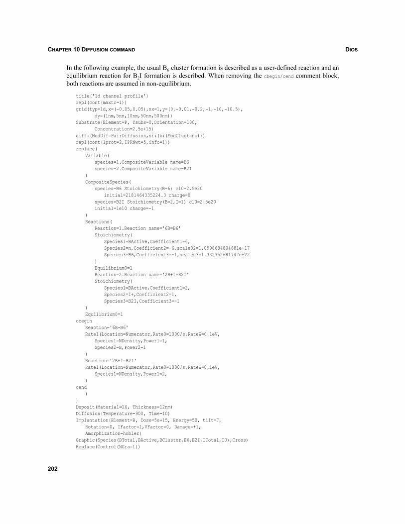
DIOSCHAPTER 10 DIFFUSION COMMAND
In the following example, the usual B6 cluster formation is described as a user-defined reaction and anequilibrium reaction for B2I formation is described. When removing the cbegin/cend comment block,both reactions are assumed in non-equilibrium.
title('1d channel profile')repl(cont(maxtr=1))grid(typ=1d,x=(-0.05,0.05),nx=1,y=(0,-0.01,-0.2,-1,-10,-10.5),
dy=(1nm,5nm,10nm,50nm,500nm))Substrate(Element=P, Ysubs=0,Orientation=100,
Concentration=2.5e+15)diff:(ModDif=PairDiffusion,si:(b:(ModClust=no)))repl(cont(lprot=2,IPRNwt=5,info=1))replace(
Variable(species=1.CompositeVariable name=B6species=2.CompositeVariable name=B2I
)CompositeSpecies(
species=B6 Stoichiometry(B=6) cl0=2.5e20initial=2181464335224.3 charge=0
species=B2I Stoichiometry(B=2,I=1) cl0=2.5e20initial=1e10 charge=-1
)Reactions(
Reaction=1.Reaction name='6B=B6'Stoichiometry(
Species1=BActive,Coefficient1=6,Species2=n,Coefficient2=-6,scale02=1.0998684804681e+17Species3=B6,Coefficient3=-1,scale03=1.332752681747e+22
)Equilibrium0=1Reaction=2.Reaction name='2B+I=B2I'Stoichiometry(
Species1=BActive,Coefficient1=2,Species2=I+,Coefficient2=1,Species3=B2I,Coefficient3=-1
)Equilibrium0=1
cbeginReaction='6B=B6'Rate1(Location=Numerator,Rate0=1000/s,RateW=0.1eV,
Species1=NDensity,Power1=1,Species2=B,Power2=1
)Reaction='2B+I=B2I'Rate1(Location=Numerator,Rate0=1000/s,RateW=0.1eV,
Species1=NDensity,Power1=2,)
cend)
)Deposit(Material=OX, Thickness=12nm)Diffusion(Temperature=900, Time=10)Implantation(Element=B, Dose=5e+15, Energy=50, tilt=7,
Rotation=0, IFactor=1,VFactor=0, Damage=+1,Amorphization=hobler)
Graphic(Species(BTotal,BActive,BCluster,B6,B2I,ITotal,I0),Cross)Replace(Control(NGra=1))
202
DIOS CHAPTER 10 DIFFUSION COMMAND
Etching(Material=OX, Remove=0.02)Diffusion(Thickness=6nm, Temperature=800, Atmosphere=HCL, cl=10)end
10.2.14 Modeling silicon germanium
10.2.14.1 Material SG
The material SG (silicon germanium) has been introduced to allow separate user-defined values in thesilicon and silicon-germanium mixed layers. In the SG material, the model will not depend on thegermanium content. The same point defect based diffusion mechanism and the same models and modelparameters are used as in silicon. The default parameters for SG have been copied from silicon. Someparameters are currently not used for SG (sometimes even if they are already defined): for example, thepoint defect parameters can not be specified for SG; the parameter values from Si are used.
10.2.14.2 Germanium in silicon
A more sophisticated modeling of germanium diffusion and interaction with dopants requiresgermanium to be introduced as a species with a concentration profile similar to a dopant such as boron.In this case the silicon-germanium layer should be modeled in Dios as a silicon layer containing a localconcentration of germanium. It is not necessary or even recommended to use an extra layer of materialSG, when applying this model, a graded transition between silicon and SG will be assumed.
The total germanium concentration can be introduced during the simulation of Implantation, Load, orDeposit commands. Together with the GeTotal, the dataset xMoleFraction is introduced into the simulation.This dataset can be exported to Mdraw and Sentaurus Device. This is done only if the user eitherprescribes the list of datasets explicitly or specifies Synonyms(SI=SG) when saving the files with Type=Mdraw.
The dopant diffusivity is modified by the strain, caused by the presence of Ge in the strained SG layer.Since no model for this strain is available in Dios, the modification of the dopant diffusivities is done asa function of the local concentration of germanium. In Dios an empirical modification of the diffusivitiesis assumed for all species:
(190)
Here D denotes the diffusivity according to the chosen diffusion model, without taking into account thegermanium content and the modified value used in the simulation with germanium. The values of Qcan be specified for each dopant species as Si(B(Q(Ge=-17eV)),Ge(Q(Ge=-40eV))). These are the onlynonzero default values. They are taken from the literature [8]. Formally, the same type of concentrationdependent diffusivity can be specified for all dopants, depending on all dopants.
D D0.042 Q Ge⋅ Total⋅–
k T c∗ n⋅ i⋅ ⋅------------------------------------------------–⎝ ⎠
⎛ ⎞exp=
D
203
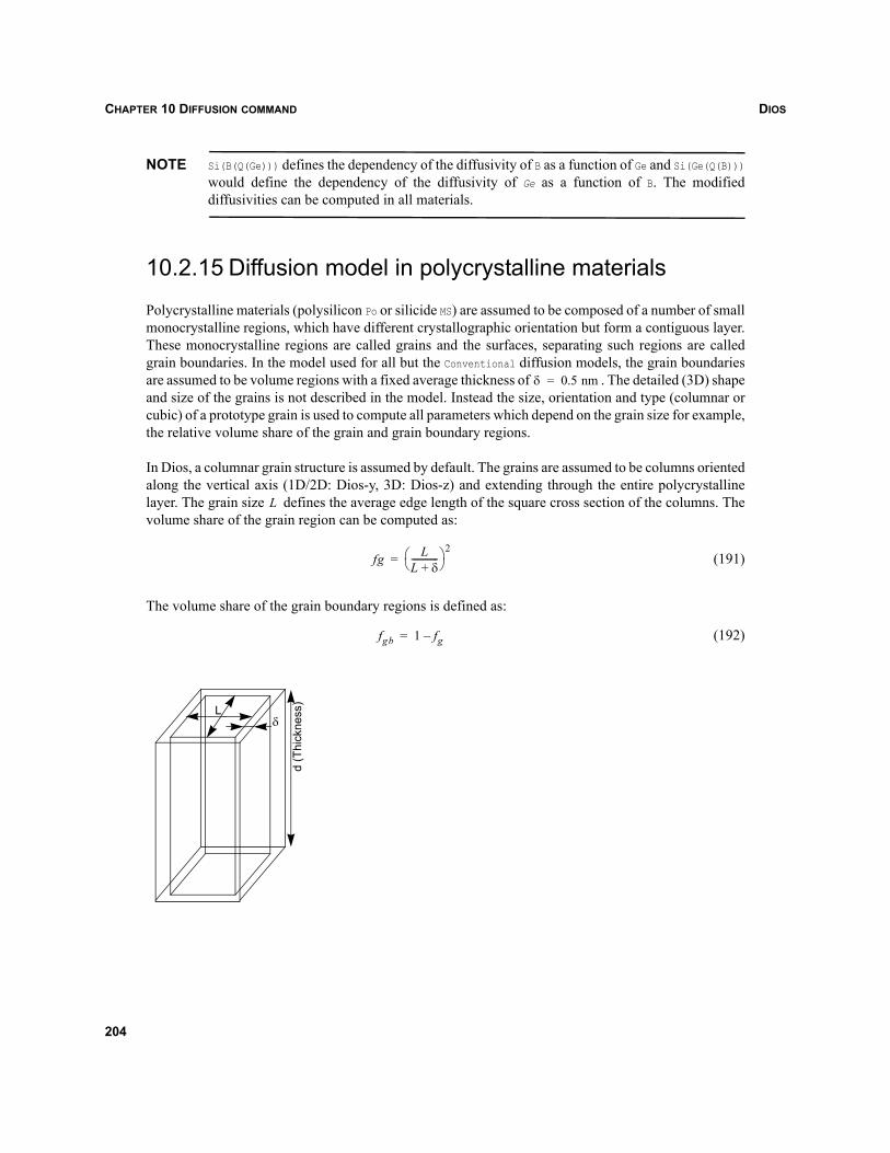
DIOSCHAPTER 10 DIFFUSION COMMAND
NOTE Si(B(Q(Ge))) defines the dependency of the diffusivity of B as a function of Ge and Si(Ge(Q(B)))would define the dependency of the diffusivity of Ge as a function of B. The modifieddiffusivities can be computed in all materials.
10.2.15 Diffusion model in polycrystalline materials
Polycrystalline materials (polysilicon Po or silicide MS) are assumed to be composed of a number of smallmonocrystalline regions, which have different crystallographic orientation but form a contiguous layer.These monocrystalline regions are called grains and the surfaces, separating such regions are calledgrain boundaries. In the model used for all but the Conventional diffusion models, the grain boundariesare assumed to be volume regions with a fixed average thickness of . The detailed (3D) shapeand size of the grains is not described in the model. Instead the size, orientation and type (columnar orcubic) of a prototype grain is used to compute all parameters which depend on the grain size for example,the relative volume share of the grain and grain boundary regions.
In Dios, a columnar grain structure is assumed by default. The grains are assumed to be columns orientedalong the vertical axis (1D/2D: Dios-y, 3D: Dios-z) and extending through the entire polycrystallinelayer. The grain size defines the average edge length of the square cross section of the columns. Thevolume share of the grain region can be computed as:
(191)
The volume share of the grain boundary regions is defined as:
(192)
δ 0.5 nm=
L
fg LL δ+------------⎝ ⎠
⎛ ⎞ 2=
fgb 1 fg–=
Lδ
d (T
hick
ness
)
204
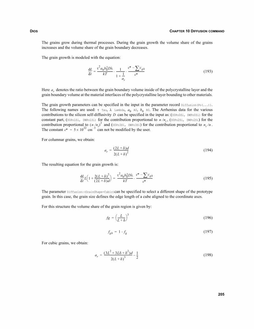
DIOS CHAPTER 10 DIFFUSION COMMAND
The grains grow during thermal processes. During the grain growth the volume share of the grainsincreases and the volume share of the grain boundary decreases.
The grain growth is modeled with the equation:
(193)
Here denotes the ratio between the grain boundary volume inside of the polycrystalline layer and thegrain boundary volume at the material interfaces of the polycrystalline layer bounding to other materials.
The grain growth parameters can be specified in the input in the parameter record Diffusion(Po(...)).The following names are used: Tau, Lambda, A0, B0. The Arrhenius data for the variouscontributions to the silicon self-diffusivity can be specified in the input as: (D0Po0Si, DWPo0Si) for theconstant part, (D0Po1Si, DWPo1Si) for the contribution proportional to , (D0Po2Si, DWPo2Si) for thecontribution proportional to and (D0Po3Si, DWPo3Si) for the contribution proportional to .The constant can not be modified by the user.
For columnar grains, we obtain:
(194)
The resulting equation for the grain growth is:
(195)
The parameter Diffusion:(GrainShape=Cubic)can be specified to select a different shape of the prototypegrain. In this case, the grain size defines the edge length of a cube aligned to the coordinate axes.
For this structure the volume share of the grain region is given by:
(196)
(197)
For cubic grains, we obtain:
(198)
tddL τ2a0b0
2DλkT
-------------------------= 1
1 1ar-----+
--------------c∗ cgb∑–
c∗--------------------------⋅ ⋅
ar
τ λ a0 b0D
n ni⁄n ni⁄( )2 ni n⁄
c∗ 5 1022× cm 3–=
ar2L δ+( )d
2 L δ+( )2------------------------=
tddLL 1 2 L δ+( )2
2L δ+( )d------------------------+⎝ ⎠
⎛ ⎞ τ2a0b02Dλ
kT-------------------------
c∗ cgb∑–
c∗--------------------------⋅=
fg LL δ+------------⎝ ⎠
⎛ ⎞ 3=
fgb 1 fg–=
ar3L2 3Lδ δ2+ +( )d
2 L δ+( )3--------------------------------------------- 1
2---–=
205
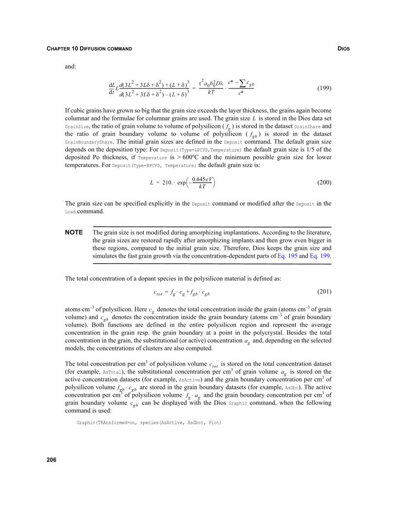
DIOSCHAPTER 10 DIFFUSION COMMAND
and:
(199)
If cubic grains have grown so big that the grain size exceeds the layer thickness, the grains again becomecolumnar and the formulae for columnar grains are used. The grain size is stored in the Dios data setGrainSize, the ratio of grain volume to volume of polysilicon ( ) is stored in the dataset GrainShare andthe ratio of grain boundary volume to volume of polysilicon ( ) is stored in the datasetGrainBoundaryShare. The initial grain sizes are defined in the Deposit command. The default grain sizedepends on the deposition type: For Deposit(Type=LPCVD,Temperature) the default grain size is 1/5 of thedeposited Po thickness, if Temperature is > 600oC and the minimum possible grain size for lowertemperatures. For Deposit(Type=NPCVD, Temperature) the default grain size is:
(200)
The grain size can be specified explicitly in the Deposit command or modified after the Deposit in theLoad command.
NOTE The grain size is not modified during amorphizing implantations. According to the literature,the grain sizes are restored rapidly after amorphizing implants and then grow even bigger inthese regions, compared to the initial grain size. Therefore, Dios keeps the grain size andsimulates the fast grain growth via the concentration-dependent parts of Eq. 195 and Eq. 199.
The total concentration of a dopant species in the polysilicon material is defined as:
(201)
atoms cm–3 of polysilicon. Here denotes the total concentration inside the grain (atoms cm–3 of grainvolume) and denotes the concentration inside the grain boundary (atoms cm–3 of grain boundaryvolume). Both functions are defined in the entire polysilicon region and represent the averageconcentration in the grain resp. the grain boundary at a point in the polycrystal. Besides the totalconcentration in the grain, the substitutional (or active) concentration and, depending on the selectedmodels, the concentrations of clusters are also computed.
The total concentration per cm3 of polysilicon volume is stored on the total concentration dataset(for example, AsTotal), the substitutional concentration per cm3 of grain volume is stored on theactive concentration datasets (for example, AsActive) and the grain boundary concentration per cm3 ofpolysilicon volume are stored in the grain boundary datasets (for example, AsGbc). The activeconcentration per cm3 of polysilicon volume and the grain boundary concentration per cm3 ofgrain boundary volume can be displayed with the Dios Graphic command, when the followingcommand is used:
Graphic(TRAnsformed=on, species(AsActive, AsGbc), Plot)
tddLLd 3L2 3Lδ δ2+ +( ) L δ+( )3+
d 3L2 3Lδ δ2+ +( ) L δ+( )3–------------------------------------------------------------------------
τ2a0b02Dλ
kT-------------------------
c∗ cgb∑–
c∗--------------------------⋅=
Lfg
fgb
L 210. 0.645eVkT
--------------------–⎝ ⎠⎛ ⎞exp⋅=
ctot fg cg fgb cgb⋅+⋅=
cgcgb
ag
ctotag
fgb cgb⋅fg ag⋅
cgb
206
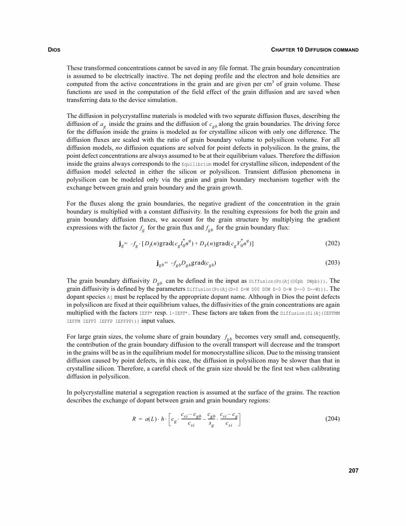
DIOS CHAPTER 10 DIFFUSION COMMAND
These transformed concentrations cannot be saved in any file format. The grain boundary concentrationis assumed to be electrically inactive. The net doping profile and the electron and hole densities arecomputed from the active concentrations in the grain and are given per cm3 of grain volume. Thesefunctions are used in the computation of the field effect of the grain diffusion and are saved whentransferring data to the device simulation.
The diffusion in polycrystalline materials is modeled with two separate diffusion fluxes, describing thediffusion of inside the grains and the diffusion of along the grain boundaries. The driving forcefor the diffusion inside the grains is modeled as for crystalline silicon with only one difference. Thediffusion fluxes are scaled with the ratio of grain boundary volume to polysilicon volume. For alldiffusion models, no diffusion equations are solved for point defects in polysilicon. In the grains, thepoint defect concentrations are always assumed to be at their equilibrium values. Therefore the diffusioninside the grains always corresponds to the Equilibrium model for crystalline silicon, independent of thediffusion model selected in either the silicon or polysilicon. Transient diffusion phenomena inpolysilicon can be modeled only via the grain and grain boundary mechanism together with theexchange between grain and grain boundary and the grain growth.
For the fluxes along the grain boundaries, the negative gradient of the concentration in the grainboundary is multiplied with a constant diffusivity. In the resulting expressions for both the grain andgrain boundary diffusion fluxes, we account for the grain structure by multiplying the gradientexpressions with the factor for the grain flux and for the grain boundary flux:
(202)
(203)
The grain boundary diffusivity can be defined in the input as Diffusion(Po(Aj(D0pb DWpb))). Thegrain diffusivity is defined by the parameters Diffusion(Po(Aj(D+0 D+W D00 D0W D-0 D-W D--0 D--W))). Thedopant species Aj must be replaced by the appropriate dopant name. Although in Dios the point defectsin polysilicon are fixed at their equilibrium values, the diffusivities of the grain concentrations are againmultiplied with the factors IEFF* resp. 1-IEFF*. These factors are taken from the Diffusion(Si(Aj(IEFFMMIEFFM IEFF0 IEFFP IEFFPP))) input values.
For large grain sizes, the volume share of grain boundary becomes very small and, consequently,the contribution of the grain boundary diffusion to the overall transport will decrease and the transportin the grains will be as in the equilibrium model for monocrystalline silicon. Due to the missing transientdiffusion caused by point defects, in this case, the diffusion in polysilicon may be slower than that incrystalline silicon. Therefore, a careful check of the grain size should be the first test when calibratingdiffusion in polysilicon.
In polycrystalline material a segregation reaction is assumed at the surface of the grains. The reactiondescribes the exchange of dopant between grain and grain boundary regions:
(204)
ag cgb
fg fgb
jg f– g DI n( )grad cgI0*nq( ) DV n( )grad cgV0
*nq( )+[ ]⋅=
jgb f– gbDgbgrad cgb( )=
Dgb
fgb
R a L( ) h cgcsi cgb–
csi--------------------⋅
cgbsg-------
csi cg–csi
-----------------⋅–⋅ ⋅=
207
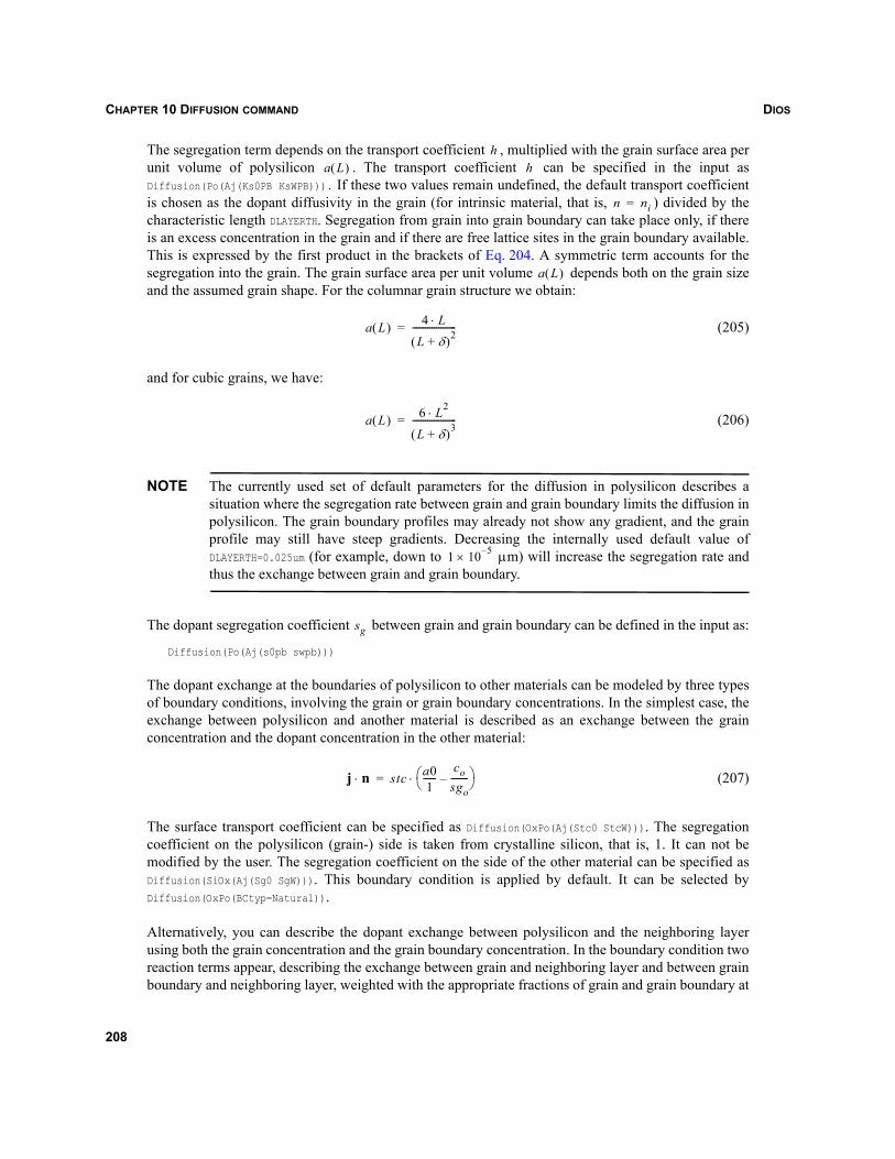
DIOSCHAPTER 10 DIFFUSION COMMAND
The segregation term depends on the transport coefficient , multiplied with the grain surface area perunit volume of polysilicon . The transport coefficient can be specified in the input asDiffusion(Po(Aj(Ks0PB KsWPB))). If these two values remain undefined, the default transport coefficientis chosen as the dopant diffusivity in the grain (for intrinsic material, that is, ) divided by thecharacteristic length DLAYERTH. Segregation from grain into grain boundary can take place only, if thereis an excess concentration in the grain and if there are free lattice sites in the grain boundary available.This is expressed by the first product in the brackets of Eq. 204. A symmetric term accounts for thesegregation into the grain. The grain surface area per unit volume depends both on the grain sizeand the assumed grain shape. For the columnar grain structure we obtain:
(205)
and for cubic grains, we have:
(206)
NOTE The currently used set of default parameters for the diffusion in polysilicon describes asituation where the segregation rate between grain and grain boundary limits the diffusion inpolysilicon. The grain boundary profiles may already not show any gradient, and the grainprofile may still have steep gradients. Decreasing the internally used default value ofDLAYERTH=0.025um (for example, down to μm) will increase the segregation rate andthus the exchange between grain and grain boundary.
The dopant segregation coefficient between grain and grain boundary can be defined in the input as:
Diffusion(Po(Aj(s0pb swpb)))
The dopant exchange at the boundaries of polysilicon to other materials can be modeled by three typesof boundary conditions, involving the grain or grain boundary concentrations. In the simplest case, theexchange between polysilicon and another material is described as an exchange between the grainconcentration and the dopant concentration in the other material:
(207)
The surface transport coefficient can be specified as Diffusion(OxPo(Aj(Stc0 StcW))). The segregationcoefficient on the polysilicon (grain-) side is taken from crystalline silicon, that is, 1. It can not bemodified by the user. The segregation coefficient on the side of the other material can be specified asDiffusion(SiOx(Aj(Sg0 SgW))). This boundary condition is applied by default. It can be selected byDiffusion(OxPo(BCtyp=Natural)).
Alternatively, you can describe the dopant exchange between polysilicon and the neighboring layerusing both the grain concentration and the grain boundary concentration. In the boundary condition tworeaction terms appear, describing the exchange between grain and neighboring layer and between grainboundary and neighboring layer, weighted with the appropriate fractions of grain and grain boundary at
ha L( ) h
n ni=
a L( )
a L( ) 4 L⋅
L δ+( )2--------------------=
a L( ) 6 L2⋅
L δ+( )3--------------------=
1 10 5–×
sg
j n⋅ stc a01
------co
sgo--------–⎝ ⎠
⎛ ⎞⋅=
208
DIOS CHAPTER 10 DIFFUSION COMMAND
the interface. This boundary condition is selected by Diffusion(SIPO(BCtyp=GBC), OXPO(BCtyp=GBC)). Theflux is modeled as:
(208)
The segregation coefficient between grain and grain boundary and the coefficient betweenpolysilicon and silicon both enter the expression for the exchange via grain boundary. They can bespecified as Diffusion(Po(Aj(S0Pb SWPb)) SiPo(Aj(Sg0 SgW))). The segregation coefficient between grainand crystalline silicon is taken again as 1.
The third type of boundary conditions balances the grain boundary concentration at the polycrystallineside with the concentration in the neighboring material:
(209)
This boundary condition can be selected with Diffusion(OxPo(BCtyp=Grain+GrainBou)).
10.2.16 Diffusion models in other materials
The dopant diffusion in other layer materials is modeled in Dios by using a simple concentrationdependent diffusivity. The dopant flux is modeled as , where the diffusivity isassumed to be a function of the concentrations. The diffusivity is assumed following [48]:
(210)
, , and are empirically defined values, the ratio is restricted in Dios to10–3–103. This model is used for all dopants. The literature values of had been selected for apredeposition from highly doped glasses. For arsenic this leads to a very high diffusion for example,through the gate oxide. Thus for arsenic the default value has been modified to undefined and internallya default value of 0 is used. The Arrhenius data for the constant diffusivity can be specified asDiffusion(Ox(Aj(Di0 DiW))) and the parameters , , and can be specified in the input asDiffusion(Ox(Aj(DDL0 DDLW CLD GDL))).
j n⋅ stcfgb c⋅ gbsgpo s⋅ g--------------------
cosgo--------–
⎝ ⎠⎜ ⎟⎛ ⎞
stcfg a0⋅
1--------------
cosgo--------–⎝ ⎠
⎛ ⎞⋅+⋅=
sgsgpo
j n⋅ stccgb
sgpo s⋅ g--------------------
cosgo--------–
⎝ ⎠⎜ ⎟⎛ ⎞
⋅=
j D ctot( )grad ctot( )–=
D Di DDL1
1CDL
Total--------------⎝ ⎠
⎛ ⎞GDL
+-------------------------------------⋅+=
DDL CDL GDL CDL Total⁄CDL
DiDDL CDL GDL
209
DIOSCHAPTER 10 DIFFUSION COMMAND
10.3 Conventional diffusion models in siliconFor the parameter Diffusion(ModDif=Conventional) a set of diffusion models can be selected which doesnot allow any point defect interaction and does not allow to solve the full Newton approximation, butuses a block Gauss–Seidel iteration to resolve the equations. For each of the dopants, the diffusivitymodel can be selected in each of the materials. In silicon, for each of the dopants the total ctot and theactive cact concentrations are distinguished. Active dopants are assumed to be electrically singly chargedand to be the only mobile dopant species. The diffusion equation is given as:
(211)
where the dopant flux j is defined as:
(212)
Here D denotes the diffusion coefficient, q the charge state (q=+1 for donors; q=–1 for acceptors) and ϕthe suitably scaled electrostatic potential.
The intrinsic carrier density in silicon is assumed to be given by:
(213)
In order to account the impact of high dopant concentrations on the band gap in silicon, a reduction ofthe band gap can be specified depending on the local total concentration for each of the dopants. As aresult an effective intrinsic density of electrons and holes is computed:
(214)
Here ni denotes the intrinsic density of silicon and the concentration of host lattice atoms( cm–3). Due to missing data, all default values of ΔEg (in the input syntax DEG) still remain zero.
10.3.1 Diffusivity in silicon
Interactions of dopant atoms and point defects (silicon interstitials I and vacancies V) are assumed to bethe driving force for the dopant diffusion in crystalline silicon. In the conventional models Dios neglectsall kinetics of point defects and describes the dopant flux by a phenomenological law Eq. 212. Allinteraction with point defects (vacancies) is contained only in the assumptions for the diffusivities. Thevacancies are assumed to exist in various charge states (Vx – neutral, V± – singly negatively or positivelycharged, and V= – doubly negatively charged). The dopant diffusivities are assumed to be given as:
(215)
c∂ tott∂
----------- jdiv+ 0=
j D cact qcact ϕgrad+grad( )–=
ni T3 2⁄ NIO NIWkT
-------------–⎝ ⎠⎛ ⎞exp=
nie ni
ΔEgctot
2kTc∗Si-------------------–
⎝ ⎠⎜ ⎟⎛ ⎞
expdopants∏=
c∗Si5 1022×
D D+ V+[ ] Dx D- V-[ ] D= V=[ ] DI I[ ]+ + + +=
210
DIOS CHAPTER 10 DIFFUSION COMMAND
If one assumes that the ionization reactions of the point defects are in equilibrium, the densities of thecharged point defects can be expressed by the concentration of the neutral defects, the electron densityn, and the effective intrinsic density . With new constants, we obtain for the diffusivities:
(216)
The diffusivities , , , and depend on the chosen diffusion model. ForDiffusion(Moddif=Conventional), the user can select the formula for these diffusivities locally per dopantand per material. Besides the special models of Fair–Tsai and Solmi, which are described in subsequentsections for silicon, there are two major types of defining the diffusivities: Suprem-2 and Suprem-3.
The diffusivities , , and for Diffusion(Si(Aj(Moddif=Suprem-3))) can be specified in theinput as Diffusion(Si(Aj(D+0 D+W Dx0 DxW D-0 D-W D--0 D--W)))).
The diffusivities for Diffusion(Si(Aj(Moddif=Suprem-2))) are defined as:
(217)
for acceptors and:
(218)
for donors. The input values can be specified as Diffusion(Si(Aj(Di0 DiW Beta Gamma))).
The values Diffusion(Si(Aj(Di0 DiW))) are used also for the case of a constant diffusivity, that is, forDiffusion(Si(Aj(Moddif=Deff))). In Eq. 217 and Eq. 218 the variable denotes the electron density and
denotes the effective intrinsic density according to Eq. 214.
NOTE For boron in silicon, the internal default values of Di0 and DiW are changed for hightemperatures (see Table 64 on page 412). The same is not done for the values used in theSuprem-3 model. This change is also not done for the models:Diffusion(Moddif=Equilibrium|LooselyCoupled|SemiCoupled|PairDiffusion) Users must change the values explicitly, for example:diff:(si(b(d+0=0.001425 d+w=2.7 dx0=0.000475 dxw=2.7)))
nie
D D+nien
------ Dx D- nnie------ D= n
nie------⎝ ⎠
⎛ ⎞ 2DI I[ ]+ + + +=
D+ Dx D- D=
D+ Dx D- D=
D Di
1 βnien
------ γnien
------⎝ ⎠⎛ ⎞
2+ +
1 β γ+ +--------------------------------------------
⎝ ⎠⎜ ⎟⎜ ⎟⎜ ⎟⎛ ⎞
⋅=
D Di
1 β nnie------ γ n
nie------⎝ ⎠
⎛ ⎞ 2+ +
1 β γ+ +--------------------------------------------
⎝ ⎠⎜ ⎟⎜ ⎟⎜ ⎟⎛ ⎞
⋅=
nnie
211
DIOSCHAPTER 10 DIFFUSION COMMAND
10.3.2 OED and oxidation-retarded diffusion (ORD) models
In the conventional models of Dios the only dependency on the silicon interstitial concentration isassumed for diffusion in oxidizing atmosphere (by default only for boron and antimony). The oxidation-enhanced diffusion (OED) of boron is computed as:
(219)
where (x,y) denotes a point in the silicon region, ( ) the closest point on an oxidation front ininterface, the velocity of that interface, computed during the oxidation and Do, voxn and lenyexperimental parameters, which can be specified in the input as Diffusion(Si(Aj(Do0 DoW Voxn) IntLen)).The OED can be interpreted as caused by additional interstitial concentration and is stored on the datasetITotal. The parameters INTDif and IntCut in Section I.4.4 on page 401 define a simple model how totransfer the local oxidation rate into the ‘interstitial concentration’ for the OED calculation. Foroxidizing ambients, containing HCl, no OED effect is simulated.
For antimony, an oxidation-retarded diffusion (ORD) is modeled:
(220)
By default, no ORD effect is assumed, that is, Do=0.
10.3.3 Diffusivity in SiGe strained layers
The simulation of dopant diffusion in strained silicon-germanium layers requires a modification of thediffusivities of all dopants, depending on the germanium concentration. In Dios an empiricalmodification of the diffusivities is assumed for all species:
(221)
Here D denotes the diffusivity according to the chosen basic diffusion model, without taking intoaccount the germanium content and the modified value used in the simulation with germanium. Thevalues of Q can be specified for each dopant species as Si(B(Q(Ge=-17eV)),Ge(Q(Ge=-40eV))). These arethe only nonzero default values. They are taken from the literature [8]. Formally the same type ofconcentration dependent diffusivity can be specified for all dopants, depending on all dopants.
NOTE Si(B(Q(Ge))) defines the dependency of the diffusivity of B as a function of Ge and Si(Ge(Q(B)))would define the dependency of the diffusivity of Ge as a function of B. The modifieddiffusivities can be computed in all materials.
DI I[ ] x y( , ) Do vΓ xΓ yΓ( , ) voxnx xΓ–( )2 y yΓ–( )2+
leny------------------------------------------------------–exp=
xΓ yΓ,vΓ
D x y,( )Dinert x y,( )
1 Do vΓ xΓ yΓ( , ) voxn+( )x xΓ–( )2 y yΓ–( )2+
leny------------------------------------------------------–
⎝ ⎠⎜ ⎟⎛ ⎞
exp⋅
---------------------------------------------------------------------------------------------------------------------------------------=
D D0.042QcGetot–
kTc*ni
------------------------------------–⎝ ⎠⎜ ⎟⎛ ⎞
exp=
D
212
DIOS CHAPTER 10 DIFFUSION COMMAND
It is not necessary and not recommended to use an extra layer of material SG, when applying this model.The germanium profile might be defined as any other doping profile by deposition, epitaxy, loading anexternal profile or using the IMPLant command.
10.3.4 Solmi model, transient-enhanced diffusivity
In order to account for implantation induced damage already in the conventional models, a further modelvariation has been implemented for boron (and formally for the other acceptor dopants). A significantlyincreased diffusivity for some time period after ion implantation is assumed. The model is used if theparameter TDK=on was specified in the Implantation command. The duration of the enhanced diffusion isdetermined from the anneal temperature by an Arrhenius law. The time can be specified asDiffusion(Si(Aj(TE0 TEW)).
The enhanced diffusivity is computed from an Arrhenius law also, but multiplied by empirical factorsdepending on implantation dose and projected range in silicon:
(222)
The diffusivity is applied for the computed time. The parameters can be specified in theDiffusion(Si(Aj(...))) records for each of the dopants. In the input is named DE0, can bespecified as DEW, can be specified as DOSE, as RP, as Exponent. For low temperatures(below TECE), the enhancement is assumed only for low concentrations. In Dios, a smooth transitionbetween ‘normal’ and enhanced diffusivity is assumed:
(223)
The parameter can be specified as FCE. In order to describe ramping processes in Dios, the end timeof the enhanced regime is determined from the integral of the temperature over the time since the ionimplantation. Moreover, for temperatures > for the entire concentration range and a very short time
an athermal diffusivity is added to the already enhanced one:
(224)
The temperature can be specified in the input as Diffusion(Si(Aj(TERTA))), the parameter canbe specified as DRTA and the duration can be specified as TRTA. For a detailed description of the model,refer to the literature [50].
10.3.5 Diffusivity in Fair–Tsai model
In Dios, an effort was made to ‘extend’ the empirical 1D approach used in TESIM-4 for phosphorus intotwo spatial dimensions. The so-called Fair–Tsai model has been implemented, which propagates localvalues of phosphorus or electron concentrations over a large domain. Computation along the 1D dopingprofile in TESIM-4 has been replaced by computations along a series of 1D cross sections orthogonal to
Denh DOenhDEenh
kT----------------–⎝ ⎠
⎛ ⎞ dosedoseenh-------------------⎝ ⎠
⎛ ⎞ EXenh RpRenh-----------⎝ ⎠
⎛ ⎞exp=
DOenh DEenhdoseenh Renh EXenh
Dboron Denh Di Denh–( )c Cenh–
FenhCenh Cenh–-----------------------------------------+=
Fenh
Tathtath
Dboronfinal Dboron Dath+=
Tath Dath
213
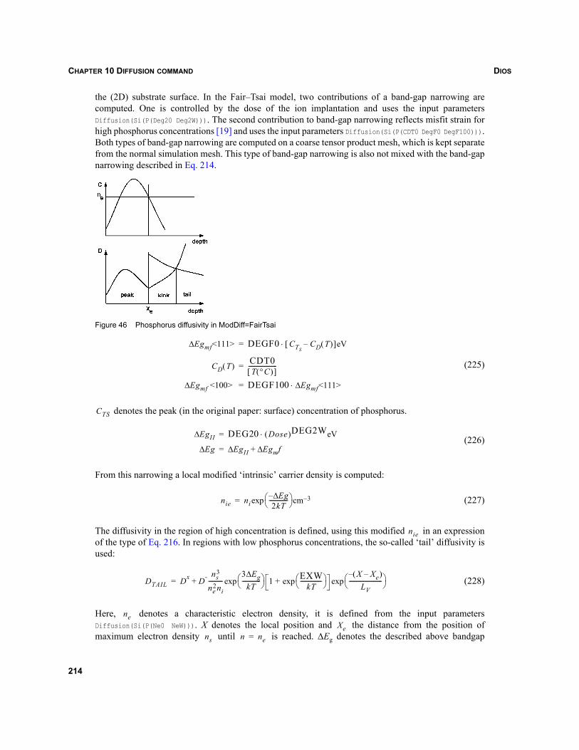
DIOSCHAPTER 10 DIFFUSION COMMAND
the (2D) substrate surface. In the Fair–Tsai model, two contributions of a band-gap narrowing arecomputed. One is controlled by the dose of the ion implantation and uses the input parametersDiffusion(Si(P(Deg20 Deg2W))). The second contribution to band-gap narrowing reflects misfit strain forhigh phosphorus concentrations [19] and uses the input parameters Diffusion(Si(P(CDT0 DegF0 DegF100))).Both types of band-gap narrowing are computed on a coarse tensor product mesh, which is kept separatefrom the normal simulation mesh. This type of band-gap narrowing is also not mixed with the band-gapnarrowing described in Eq. 214.
Figure 46 Phosphorus diffusivity in ModDiff=FairTsai
(225)
denotes the peak (in the original paper: surface) concentration of phosphorus.
(226)
From this narrowing a local modified ‘intrinsic’ carrier density is computed:
(227)
The diffusivity in the region of high concentration is defined, using this modified in an expressionof the type of Eq. 216. In regions with low phosphorus concentrations, the so-called ‘tail’ diffusivity isused:
(228)
Here, denotes a characteristic electron density, it is defined from the input parametersDiffusion(Si(P(Ne0 NeW))). X denotes the local position and the distance from the position ofmaximum electron density until is reached. ΔEg denotes the described above bandgap
Egmf<111>Δ DEGF0 CTSCD T( )–[ ]eV⋅=
CD T( ) CDT0T °C( )[ ]
--------------------=
Egmf <100> Δ DEGF100 Egmf<111>Δ⋅=
CTS
EgIIΔ DEG20 Dose( )DEG2WeV⋅=
EgΔ EgIIΔ EgmfΔ+=
nie niEgΔ–
2kT-------------⎝ ⎠
⎛ ⎞ cm 3–exp=
nie
DTAIL Dx D- ns3
ne2ni
----------3 EgΔ
kT-------------⎝ ⎠
⎛ ⎞exp 1 EXWkT
---------------⎝ ⎠⎛ ⎞exp+
X Xe–( )–LV
-----------------------⎝ ⎠⎛ ⎞exp+=
neXe
ns n ne=
214
DIOS CHAPTER 10 DIFFUSION COMMAND
narrowing, the exponent EXW and the decay length into the bulk can be specified in the input asDiffusion(Si(P(ExW LV))). For intermediate concentrations and depth range the ‘peak’-diffusivity ismultiplied by (( )/(n))2, until the modified value exceeds , further below the tail diffusivity
is used (see Figure 46 on page 214).
In order to obtain results similar to the model implemented in TESIM-4, in addition to the Fair–Tsaidiffusion model, one has to select a clustering model for phosphorus.
The model switch ModDiff=FairTsai can be used for phosphorus and boron. In this case, the enhancedphosphorus tail diffusivity is used to empirically ‘model’ a (nonlocal) emitter push effect.
The boron diffusivity is multiplied with an enhancement factor (the ratio of the phosphorus taildiffusivity and the ‘intrinsic’ phosphorus diffusivity):
(229)
10.3.6 Clustering models for conventional diffusion
The difference between total and substitutional (active) concentrations for each of the dopants E isassumed to be the result of a clustering reaction. Two types of clustering models have been implementedin Dios, simple cut-off of active concentrations and clustering reactions leading to nonlinear relationshipbetween active and total concentration. In the simple models ModClust=Table | Solubility the totalconcentration is cut at the maximum solubility level and used as active concentration. For ModClust=Tablethe solubility level is defined according to the temperature from a hard coded internal lookup table. ForModClust=Solubility the solubility level is defined by an arrhenius law from CL0 and CLW as forModClust=OneElectron.
For the clustering models ModClust=ZeroElectron| OneElectron| MElectron, a clustering reaction isassumed:
(230)
The clustering reaction is assumed to be permanently in equilibrium. From the mass action law, oneobtains:
(231)
where denotes the reaction constant and denotes either the electron or hole concentrations,depending on the charge of the substitutional dopant (n for donors, p for acceptors).
LV
ne DTAILDTAIL
Dboronpush Dboron
DTAILDi
---------------⋅=
mEq kn q– Emq m k–( )⇔+
ctot cact mkeq cact( )m rnp( )k+=
keq rnp
215
DIOSCHAPTER 10 DIFFUSION COMMAND
The carrier concentrations and the electrostatic potential can be computed by assuming Boltzmanndistributions for electrons and holes, assuming the electron hole recombination in equilibrium, andassuming that the space charge (including immobile but eventually charged clusters ( ), butneglecting charged point defects) vanishes everywhere:
(232)
From Eq. 212 and Eq. 232:
(233)
It remains to express and as a function of the total densities . This is performed usingEq. 231 and Eq. 232, these equations couple the diffusion equations for the various dopants in a stronglynonlinear way. Assume for a moment, that only one dopant exists and the number m+k is known.
The following cases are admitted:
(234)
For ModClust=NO, one obtains:
(235)
For ModClust=OneElectron from Eq. 232, one has:
(236)
which can be resolved only for:
(237)
The parameter CL defines the solid solubility for the active dopant concentration and can be specifiedby an Arrhenius relation via the parameters Diffusion(Si(Aj(CL0 CLW))).
The equilibrium constant is defined as:
(238)
m k≠
n nie ϕ( ) , exp= p nie ϕ–( ) ,exp=
np nie2 ,= n p– q cact
m k–m
------------- ctot cact–( )+⎝ ⎠⎛ ⎞
dopants∑=
j Drnp------- cactrnp( )grad–=
cact rnp ctot
MODClust
NO, no clusteringZeroElectron, k 0=OneElectron, k 1=
MElectron, k m=⎩⎪⎪⎨⎪⎪⎧
=
cact ctot , = rnpctot2
-------- ni2
ctot2
--------⎝ ⎠⎛ ⎞
2++=
rnp2 1 m k–( )keqcact
m–( ) ni2 cactrnp+=
cact CL m k 2–+( )keq( )1 1 m– k–( )⁄:=≤
keq
keq1
m k 2–+----------------------CL1 m– k–=
216
DIOS CHAPTER 10 DIFFUSION COMMAND
The same formula is used to define the equilibrium constants for the clustering modelsModClust=ZeroElectron, MElectron, which strictly speaking do not posses a solid solubility level. If severaldopants exist, ModClust=NO, ZeroElectron, Solubility, Table can be used for all of them,ModClust=OneElectron, MElectron can be used only for one of the dopants.
A major difference between the clustering models results from the different charge state that is assumedfor the clusters. As described, all charged particles, active atoms and (partially) charged clusters appearin the charge neutrality balance that is, in the right hand side of the Poisson equation. When computingthe net concentration Net the substitutional (active) atoms and the charged clusters are summed up,multiplied with their appropriate charge numbers. The dataset NetActive provides just the sum of thesubstitutional dopants, multiplied with the charge numbers. This concentration is used when saving filesfor the device simulator Sentaurus Device. Both Net and NetActive vanish in materials where the chargenumbers vanish (for example, OX, NI).
NOTE For ModClust=ZeroElectron, the clusters are fully charged.
The parameter Diffusion(MaximizeSolubility=on/off) can be used to control if the solid solubility ismaximized during the anneal processes or if the solid solubility is allowed to increase and decrease. Bydefault, the solid solubility level CL for each of the dopants is kept fixed at the highest temperature, thedopant has seen in the simulation. Since only equilibrium clustering models are used in the Conventionalsolver, this proved to account better for the slower declustering dynamics in ramp down processes.
10.3.7 Conventional diffusion model in polysilicon
Polycrystalline silicon (PO) is composed of a large number of small silicon monocrystals, which form acontinuous layer, but have different crystallographic orientations. This orientation mismatch (crystaldefect) is called ‘grain boundaries’ and the monocrystals are called ‘grains.’ The grains resemble convexpolyhedra. The grain boundaries are piecewise planar and are treated in the Conventional diffusion modelin Dios as 2D objects in the 3D polycrystalline material (or more precisely as 1D lines, formed by theintersections of the grain boundaries with the simulation domain). In this model the ‘volume share’ ofthe grain boundaries in the volume of the sample is exactly zero. The area of grain boundary per volumepolysilicon is used to characterize the grain structure.
Experimental results show a very large ratio of the diffusivities (Dpoly) in polysilicon and inmonocrystalline Si (Dmono) (for As-diffusion, 2.1016 cm–2 As, 950oC, 30 minutes: Dpoly/Dmono=104 [44]).
Polysilicon is decomposed into two fractions: grains (g) and grain boundary (gb). The enhanceddiffusion in polysilicon is attributed to a very fast dopant diffusion along the grain boundaries. Inprinciple the diffusion equations have to be solved in N+1 areas: N not connected to each other grainsand the connecting all together grain boundary area. Of course for any given polysilicon sample the grainstructure is not known, it is truly 3D and it changes with time. So one has to use rather averaged valuesfor an ensemble of possible grain configurations representing the technological situation, and averagingthe grain structure in Dios z-direction which is neglected in the 2D simulation. One may assume a certainprobability, that each bulk element of the polysilicon sample contains grains as well as a certain amountof grain boundary area. In the limit case, the bulk element shrinks to a point and one has to solve for each
217
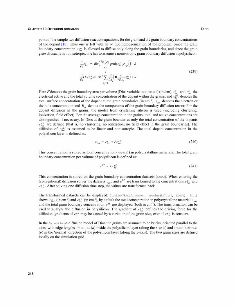
DIOSCHAPTER 10 DIFFUSION COMMAND
point of the sample two diffusion-reaction equations, for the grain and the grain boundary concentrationsof the dopant [10]. Thus one is left with an ad hoc homogenization of the problem. Since the grainboundary concentration is allowed to diffuse only along the grain boundaries, and since the graingrowth usually is nonisotropic, one has to assume a nonisotropic grain boundary diffusion in polysilicon:
(239)
Here F denotes the grain boundary area per volume (Dios variable: GrainShare) (in /cm), and theelectrical active and the total volume concentration of the dopant within the grains, and denotes thetotal surface concentration of the dopant at the grain boundaries (in cm–2). denotes the electron orthe hole concentration and denote the components of the grain boundary diffusion tensor. For thedopant diffusion in the grains, the model from crystalline silicon is used (including clustering,ionization, field effect). For the average concentration in the grains, total and active concentrations aredistinguished if necessary. In Dios at the grain boundaries only the total concentration of the dopants
are defined (that is, no clustering, no ionization, no field effect in the grain boundaries). Thediffusion of is assumed to be linear and nonisotropic. The total dopant concentration in thepolysilicon layer is defined as:
(240)
This concentration is stored as total concentration (AsTotal) in polycrystalline materials. The total grainboundary concentration per volume of polysilicon is defined as:
(241)
This concentration is stored on the grain boundary concentration datasets (AsGbc). When entering the(conventional) diffusion solver the datasets and are transformed to the concentrations and
. After solving one diffusion time step, the values are transformed back.
The transformed datasets can be displayed: Graphic(TRAnsformed=on, species(AsTotal, AsGbc), Plot)
shows (in cm-3) and (in cm-2), by default the total concentration in polycrystalline material and the total grain boundary concentration are displayed (both in cm-3). The transformation can beused to analyze the diffusion in polysilicon. The gradient of defines the driving force for thediffusion, gradients of may be caused by a variation of the grain size, even if is constant.
In the Conventional diffusion model of Dios the grains are assumed to be bricks, oriented parallel to theaxes, with edge lengths GrainSize (a) inside the polysilicon layer (along the x-axis) and GrainsizeNormal(b) in the ‘normal’ direction of the polysilicon layer (along the y-axis). The two grain sizes are definedlocally on the simulation grid.
ctotgb
t∂∂ ctot
g Dg c( )rnp
-------------- cactg rnp( )grad⎝ ⎠
⎛ ⎞div R–=
t∂∂ Fctot
gb( ) Dgbxi∂∂ Di j xj∂
∂ ctotgb
⎝ ⎠⎛ ⎞
i,j=1
3
∑ R+=
cactg ctot
g
ctotgb
rnpDi j
ctotgb
ctotgb
ctot ctotg Fctot
gb+=
cgb Fctotgb=
ctot cgb ctotg
ctotgb
ctotg ctot
gb ctotcgb
ctotgb
cgb ctotgb
218
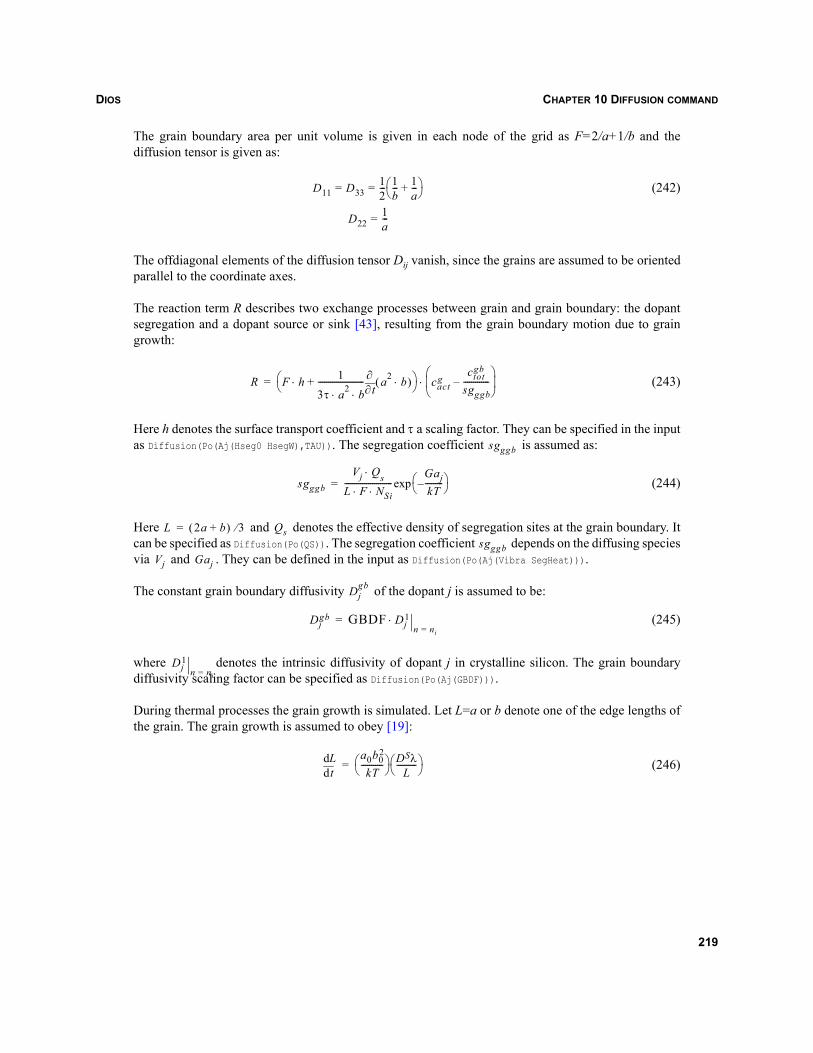
DIOS CHAPTER 10 DIFFUSION COMMAND
The grain boundary area per unit volume is given in each node of the grid as F=2/a+1/b and thediffusion tensor is given as:
(242)
The offdiagonal elements of the diffusion tensor Dij vanish, since the grains are assumed to be orientedparallel to the coordinate axes.
The reaction term R describes two exchange processes between grain and grain boundary: the dopantsegregation and a dopant source or sink [43], resulting from the grain boundary motion due to graingrowth:
(243)
Here h denotes the surface transport coefficient and τ a scaling factor. They can be specified in the inputas Diffusion(Po(Aj(Hseg0 HsegW),TAU)). The segregation coefficient is assumed as:
(244)
Here and denotes the effective density of segregation sites at the grain boundary. Itcan be specified as Diffusion(Po(QS)). The segregation coefficient depends on the diffusing speciesvia and . They can be defined in the input as Diffusion(Po(Aj(Vibra SegHeat))).
The constant grain boundary diffusivity of the dopant j is assumed to be:
(245)
where denotes the intrinsic diffusivity of dopant j in crystalline silicon. The grain boundarydiffusivity scaling factor can be specified as Diffusion(Po(Aj(GBDF))).
During thermal processes the grain growth is simulated. Let L=a or b denote one of the edge lengths ofthe grain. The grain growth is assumed to obey [19]:
(246)
D11 D3312--- 1
b--- 1
a---+⎝ ⎠
⎛ ⎞= =
D221a---=
R F h⋅ 13τ a2 b⋅⋅-----------------------
t∂∂ a2 b⋅( )+⎝ ⎠
⎛ ⎞ cactg
ctotgb
sgggb-------------–
⎝ ⎠⎜ ⎟⎛ ⎞
⋅=
sgggb
sgggb
Vj Q⋅ sL F NSi⋅ ⋅------------------------
GajkT---------–⎝ ⎠
⎛ ⎞exp=
L 2a b+( ) 3⁄= Qssgggb
Vj Gaj
Djgb
Djgb GBDF Dj
1n ni=
⋅=
Dj1
n ni=
tddL a0b0
2
kT-----------⎝ ⎠
⎛ ⎞ DSλL
----------⎝ ⎠⎛ ⎞=
219
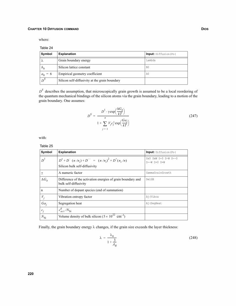
DIOSCHAPTER 10 DIFFUSION COMMAND
where:
describes the assumption, that microscopically grain growth is assumed to be a local reordering ofthe quantum mechanical bindings of the silicon atoms via the grain boundary, leading to a motion of thegrain boundary. One assumes:
(247)
with:
Finally, the grain boundary energy λ changes, if the grain size exceeds the layer thickness:
(248)
Table 24
Symbol Explanation Input: Diffusion(Po(
Grain boundary energy Lambda
Silicon lattice constant B0
Empirical geometry coefficient A0
Silicon self-diffusivity at the grain boundary
Table 25
Symbol Explanation Input: Diffusion(Po(
Silicon bulk self-diffusivity
Dx0 DxW D-0 D-W D--0 D--W D+0 D+W
A numeric factor GammaGrainGrowth
Difference of the activation energies of grain boundary and bulk self-diffusivity
DelGB
n Number of dopant species (end of summation)
Vibration entropy factor Aj(Vibra
Segregation heat Aj(SegHeat
Volume density of bulk silicon ( cm–3)
λ
b0
a0 6=
DS
DS
DSD1 γ⋅
GbΔkT
----------⎝ ⎠⎛ ⎞exp
1 Vjcj1
GajkT---------⎝ ⎠
⎛ ⎞expj 1=
n
∑+
-------------------------------------------------------=
D1 Dx D–+ n ni⁄( ) D ––+ = n ni⁄( )2 D+ ni n⁄( )+
γ
ΔGb
Vj
Gaj
cj cactg NSi⁄
NSi 5 1022×
λλ0
1 3AR------+
----------------=
220
DIOS CHAPTER 10 DIFFUSION COMMAND
If the layer has a constant thickness Y and if it is parallel to the x-z plane, then:
(249)
Interfaces of polysilicon regions to other materials may be interpreted as pure grain boundary. Thefunction GrainShare (grain boundary area per unit volume) can not be interpreted at interfaces, thuscausing difficulties when displaying the grain boundary concentration as volume concentration atmaterial interfaces.
The dopant exchange at the boundaries of polysilicon to other materials can be modeled by two types ofboundary conditions for the grain and grain boundary concentrations. In the first type of boundaryconditions, the grain boundary concentration is subjected to homogeneous Neumann conditions and theexchange between polysilicon and other materials is described by the exchange between the grainconcentration and the dopant concentration in the other material.
(250)
This boundary condition is applied by default, for example: Diffusion(OxPo(BCtyp=FluxParameter)). Thesurface transport coefficient stc is defined per boundary sort and dopant as Diffusion(OxPo(Aj(STC0STCW))). For consistency reasons, the segregation coefficients are defined only for the boundaries tosilicon and for each dopant as: Diffusion(SiPo(Aj(SG0 SGW))).
Alternatively, you can describe the dopant exchange between polysilicon and the neighboring layersusing the grain boundary concentration. In the boundary condition two reaction terms appear, onedescribing the exchange between grain and grain boundary and one describing the exchange betweengrain boundary and neighboring layer. This boundary condition can be used, to model a local dopantpeak at the interface between polysilicon and neighboring layer. It is chosen for each boundary sort byDiffusion(SIPO(BCtyp=GBC), OXPO(BCtyp=GBC)).
(251)
(252)
(253)
The transport and the segregation coefficients for the exchange between grain and grain boundary aretaken from the volume segregation reaction (see Eq. 243 and Eq. 244).
AR
0.5 Y F⋅ 1–( ),⋅ b Y<
0.5 Y 2a--- 1
Y---+⎝ ⎠
⎛ ⎞⋅ 1–⎝ ⎠⎛ ⎞ ,⋅ b Y>
⎩⎪⎨⎪⎧
=
j n stcctot
g
sgpo----------
cosgo--------–
⎝ ⎠⎜ ⎟⎛ ⎞
⋅=⋅
jo no stccosgo--------
ctotgb
sgpo sgggb⋅-----------------------------–
⎝ ⎠⎜ ⎟⎛ ⎞
⋅=⋅
jg npo hctot
g
sgpo----------
ctotgb
sgpo sgggb⋅-----------------------------–
⎝ ⎠⎜ ⎟⎛ ⎞
⋅=⋅
jg npo jo no jg npo⋅–⋅–=⋅
221
DIOSCHAPTER 10 DIFFUSION COMMAND
Silicide layers are assumed to have a polycrystalline structure. The polysilicon dopant diffusion modelis applied there. The diffusivities can be specified separately, but currently the grain growth parametersof polysilicon are used.
10.3.7.1 Using another diffusion model in polysilicon
In the conventional diffusion model, it is possible to select a simpler diffusion model in polysilicon. Youcan specify:
Diffusion:(PO(As(ModDiff=Suprem-2),P(ModDiff=Suprem-2),B(ModDiff=Suprem-2)
))
Then, no grain boundary concentrations are introduced and only a single diffusion equation is solved.To account for the high dopant transport in polysilicon, the diffusivities computed according to theselected models are multiplied by the factors GBDF.
10.3.8 Conventional diffusion models in other materials
The dopant flux in other materials is assumed as: . For Diffusion(Ox(As(ModDiff=DEFF)))the diffusivity D is assumed to be constant and given by and Arrhenius relation. The diffusivity is givenby Diffusion(Ox(Aj(Di0 DiW))).
For Diffusion(Ox(As(ModDiff=DC))), following [48], the diffusivities depend on the total dopantconcentration:
(254)
DDL, CDL and GDL are empirically defined values, the ratio CDL/Total is restricted in Dios to 10–3–103.This model is used by default for boron and phosphorus in oxide. The literature values of CDL had beenchosen for a predeposition from highly doped glasses. For arsenic, this leads to a very high diffusion,for example, through the gate oxide. Thus for arsenic, ModDiff=DEFF is used. The Arrhenius data for theconstant diffusivity can be specified as Diffusion(Ox(Aj(Di0 DiW))) and the parameters , ,and can be specified in the input as Diffusion(Ox(Aj(DDL0 DDLW CLD GDL))).
10.4 ConvectionThe diffusion equations formulated until now for the various materials, cover situations with fixedboundaries. If there is a flow of a given velocity field v(x,y) in the layers, (for example, caused byoxidation or silicidation) there is an additional convective transport of dopants, that has to be taken intoaccount.
j D– gradctot=
D Di DDL1
1CDL
Total--------------⎝ ⎠
⎛ ⎞GDL
+-------------------------------------+=
Di DDL CDLGDL
222
DIOS CHAPTER 10 DIFFUSION COMMAND
For example, Eq. 211 transforms into:
(255)
For divv=0, this can be rewritten as:
(256)
Consequently, in all diffusion equations, the diffusion flux j must be replaced by the sum of the diffusionand convection fluxes. The problem becomes even more complicated if you take into account thediscontinuity of the velocities at material interfaces as they usually occur during oxidation orsilicidation. Various numeric approaches have been tested in Dios, in order to account for the convectionflux during oxidation (see parameter Control(Convection...) in Section Q.2 on page 554). Theconvective flux may even dominate the diffusive transport, for example, in oxide and nitride layers. Thebest results, with respect to numeric stability, have been achieved until now with a separation ofconvection and diffusion steps Convection=Regrid. In this case the convective terms in the bulk regions aswell as at the moving interfaces are treated together with the re-gridding step, that is used to adjust thegrid to the changing with time layer structure.
10.5 Boundary conditionsAt the material interfaces the total dopant fluxes are balanced. In case of moving boundaries, anadditional convection flux, proportional to the velocity of the boundary motion, occurs: .
Furthermore, the interface might carry an independent surface density u, which may be submitted todiffusive or convective transport along the interface:
(257)
Here denotes the outer unit normal with respect to region i. A second condition results from dopantsegregation. One may require either the segregation equilibrium
(258)
or regard the deviation from the equilibrium as the driving force for the flux across the interface (fluxparameter condition):
(259)
(260)
ctot∂t∂
----------- v ctotgrad⋅ jdiv+ + 0=
ctot∂t∂
----------- j ctotv+( )div+ 0=
j ctot+ v ctot– vΓ
u· divs js( )+ j1 ctot1 v1 ctot
1 vΓ–+( ) n1⋅ j2 ctot2 v2 ctot
2 vΓ–+( ) n2⋅+=
ni
ctot1 u
sg1--------= ctot
2 usg2--------=
j1 ctot1 v1 ctot
1 vΓ–+( ) n1⋅ h1 ctot1 u
sg1--------–⎝ ⎠
⎛ ⎞⋅=
j2 ctot2 v2 ctot
2 vΓ–+( ) n2⋅ h2 ctot2 u
sg2--------–⎝ ⎠
⎛ ⎞⋅=
223
DIOSCHAPTER 10 DIFFUSION COMMAND
In Dios, no independent surface species are assumed at all interfaces. Then, u → 0, sg1 → 0, sg2 → 0,sg12:= sg1 / sg2.
For segregation equilibrium one obtains in the inert case:
(261)
(262)
and for flux parameter conditions one obtains:
(263)
(264)
In the conventional diffusion models in Dios, mixed boundary conditions are used. The convectionterms (during oxidation, silicidation, epitaxy) are handled according to the chosen grid strategy and tothe parameters BDryflux, BDRYValue and Convection in the Control parameter record. By default theconvection terms are handled outside of the diffusion solver. For special applications, special types ofboundary conditions are implemented and reported in the appropriate sections (prebake, epitaxy,diffusion in polysilicon). The following general types of boundary conditions can be used.
BCTyp=FluxParameter
Natural boundary conditions (mixed boundary condition). The total dopant fluxes at the interfaces arebalanced Eq. 263 and Eq. 264. The fluxes are assumed to be proportional to the deviation from thesegregation equilibrium. This boundary condition is used by default at the interfaces between twomaterials. At boundaries to polycrystalline materials the dopant fluxes across the interface are definedby the dopant concentrations in the grain and in the other material, by the segregation coefficient andflux parameter. A vanishing flux is assumed for the grain boundary concentrations. This is justified forlarger diffusion times, when the segregation equilibrium grain-grain boundary concentration is settledin the vicinity of the interface inside the polysilicon.
BCTyp=3PhaseSegregat
Allows dopants to segregate to the interface. The additional interface equation is described inSection 10.2.12.5 on page 196. This BCTyp simulates dose loss because those dopants that segregate tothe interface are considered inactive.
j1 ctot1 v1 ctot
1 vΓ–+( ) n1⋅ j2 ctot2 v2 ctot
2 vΓ–+( ) n2⋅+ 0=
ctot1
ctot2
sg12----------=
j1 ctot1 v1 ctot
1 vΓ–+( ) n1⋅ h12 ctot1
ctot2
sg12----------–
⎝ ⎠⎜ ⎟⎛ ⎞
=
j2 ctot2 v2 ctot
2 vΓ–+( ) n2⋅ h– 12 ctot1
ctot2
sg12----------–
⎝ ⎠⎜ ⎟⎛ ⎞
=
224
DIOS CHAPTER 10 DIFFUSION COMMAND
BCTyp=HomNeumann
Vanishing fluxes, no transfer across the interfaces. This is chosen by default at the left/right/bottomboundaries, but can be specified at all boundaries.
BCTyp=Natural
Natural boundary condition (mixed boundary condition). The normal flux across an outer surface is modeled. This boundary condition is used for oxidation (see below) and at the outer
surfaces to gas (predeposition, evaporation)).
BCTyp=Dirichlet
Prescribe the value of the solution at the boundary: . This can be used at the outer surface of amaterial to gas (predeposition, evaporation), or at the bottom boundary to enforce a fixed doping level.This can also be used for the electrostatic potential in the point defect solver.
BCTyp=1Dcontinuation
At the left/right boundaries, a 1D problem is solved by extracting the vertical positions of the boundarymesh points. The solution values are then prescribed as Dirichlet boundary values to the 2D problem.This should not be used any more.
BCTyp=Segregation (Eq. 261 and Eq. 262)
This is disabled and internally replaced by BCTyp=FluxParameter.
BCTyp=SURDensity
This type of boundary condition is internally used for prebake and epitaxy simulation. It is disabled forthe other processes.
BCTyp=GBC
This type of boundary condition can be selected at the boundaries of polycrystalline material. Forinterfaces to polycrystalline regions and ModDiff=POLY, the dopant fluxes from grain and grain boundaryare balanced with the dopant flux from the other material. Dopant segregation reactions at the interfaceare assumed both between the grain boundary concentration and the concentration in the other material,and between grain boundary concentration and grain concentration. This boundary condition may causea dopant peak at the interface. A special version of this boundary condition is implemented for the pointdefect solver (see Eq. 208).
BCTyp=DiriTotNoPairs
This boundary condition can be used for pair diffusion. The total concentration without the pairconcentration is prescribed. A nonlinear Dirichlet condition is applied: . The real boundary
j n⋅ h c c∗–( )=
c c∗=
F c( ) 0=
225
DIOSCHAPTER 10 DIFFUSION COMMAND
value usually is not prescribed explicitly, but depends on the electron density and can be computed onlyduring the Newton iteration.
BCTyp=DiriTotPairs
This boundary condition can be used for pair diffusion. The total concentration including the pairconcentration is prescribed. A nonlinear Dirichlet condition is applied: . The real boundaryvalue usually is not prescribed explicitly, but depends on the electron density and can be computed onlyduring the Newton iteration.
BCTyp=DiriNeutral
This boundary condition can be used for pair diffusion. The substitutional concentration, resp. theneutral unpaired point defect concentration is prescribed. A nonlinear Dirichlet condition is applied:
. The real boundary value usually is not prescribed explicitly, but depends on the electrondensity and can be computed only during the Newton iteration. Not all types of boundary condition canbe selected at all interfaces, for all species, and all diffusion models.
In particular, the following rules are important:
The same type of boundary condition is applied for all dopants at a boundary sort.
For each boundary sort, the type of boundary condition for the Poisson equation and for each typeof point defects (I and V) can be chosen independently.
The equilibrium concentrations and the surface transport coefficients can be chosen individually perdopant species and per boundary sort.
10.5.1 Coupled dopant–point defect diffusion
Different boundary conditions can be specified for interstitials, vacancies, dopants and for theelectrostatic potential. The left/right sides of the simulation domain are always handled as symmetrylines.
The type of boundary condition for all dopants is defined as for the conventional diffusion, according tothe grid strategy. For NewDiff=0, in the grid command. For NewDiff=1 with the parameter BCtyp for eachboundary sort:
Diffusion(SIOX(BCtyp=HomNeumann|FluxParameter))
On the outer boundary of the simulation domain, Dirichlet conditions can be chosen. Three differenttypes are admitted: one may prescribe the total concentration, the total concentration without pairs or thesubstitutional concentration. This can be used, for example, to simulate predeposition. By default, on theouter boundary natural boundary conditions are chosen, that is, an incorporation/evaporation processwith finite rate is modeled:
(265)
F c( ) 0=
F c( ) 0=
j n⋅ k Ajqj[ ]
Aj*qj[ ]
–( )=
226
DIOS CHAPTER 10 DIFFUSION COMMAND
The reaction rate k (flux parameters) can be specified for each boundary sort and each dopant asDiffusion(SiOx(Aj(Stc0 StcW))), the equilibrium value is specified for each dopant as:Gas(As(Cequi)). It is cut off internally at the (temperature dependent) solid solubility:
(266)
The boundary conditions for the electrostatic potential are used only, if Poisson equation is solvedDiffusion(Poisson=on). The boundary conditions are selected by Diffusion(SIOX(U( BCtyp))). By default,homogeneous Neumann conditions are used at the external boundaries and
at internal interfaces. Alternatively, a Dirichlet condition can bespecified and the value of the potential can be prescribed (as Diffusion(SIOX(U(Value)))).
Point defect equations are solved only in silicon. At the boundaries to other materials the type ofboundary condition for the point defects can be specified for each boundary sort as:
Diffusion(SIOX(I(BCtyp=Natural|DiriNeutral|HomNeumann|DiriTotPairs|DiriTotNoPairs)Diffusion(SIOX(V(BCtyp=Natural|DiriNeutral|HomNeumann|DiriTotPairs|DiriTotNoPairs)
Homogeneous or inhomogeneous Neumann conditions or one of the three different types of Dirichletconditions can be selected. One can prescribe the concentration of neutral unpaired point defects(DiriNeutral). This is the default. Alternatively the concentration of total point defects can be prescribed,either including also the dopant-point defect pairs (DiriTotPairs), or not including the dopant-defectpairs (DiriTotNoPairs). The default value is prescribed by the equilibrium concentration of neutralinterstitials, which is given by an Arrhenius law as Diffusion(Si(I(C0STAR CWSTAR))) andDiffusion(Si(V(C0STAR CWSTAR))). At the bottom boundary (URand) of the substrate, by default, no flux isassumed. When simulating the entire wafer one might enforce the same boundary condition(DiriNeutral) as on the top silicon surface.
To keep consistency, by default (modified) Dirichlet boundary conditions for the neutral unpaired pointdefects are used also for the oxidation. The (local) equilibrium value at the interface is chosen as afunction of the (local) oxidation rate, to account for oxidation enhanced diffusion:
(267)
with:
(268)
and:
(269)
Aj*qj[ ]
Aj*qj[ ]
min Cequi Cl0 e⋅ xp ClWkT
-------------–( ),⎝ ⎠⎛ ⎞=
εgrad ϕ( ) n 0=⋅ε+grad ϕ+( ) n+ ε-grad ϕ-( ) n-⋅+ 0=⋅
c∗ox c= ∗ 1 Fox F⋅ dopvox n⋅
1 A·
min---------
-------------------
⎝ ⎠⎜ ⎟⎜ ⎟⎜ ⎟⎛ ⎞ Pox
+
⎝⎜⎜⎜⎛
⎠⎟⎟⎟⎞
Fdopm 2– m 1– 1 m1 m2+ + + +
m 2– q2 m 1– q1 1 m1q 1– m2q 2–+ + + +-----------------------------------------------------------------------------------------=
q nni----⎝ ⎠
⎛ ⎞ PotOx=
227
DIOSCHAPTER 10 DIFFUSION COMMAND
where and are model parameters; they have been adjusted to fit the OED effect,assumed in the conventional diffusion. The coefficients can be specified in the input asDiffusion(Si(I(Fox0 FoxW Pox0 PoxW PotOx))). The coefficients , , and are defined by thecoefficients Diffusion(Si(I(MM0 MMW M0 MW P0 PW PP0 PPW))). The parameter PotOx has been empiricallyfitted to adjust the OED effect for high doping concentrations.
Alternatively to the Dirichlet boundary conditions, for Diffusion(SIOX(I(BCTyp=NAtural))), the interstitialrecombination at the boundaries can be modeled by a reaction term:
(270)
(271)
During oxidation the recombination rate is modified locally depending on the local oxidation rate.Two different types of the interstitial generation term can be chosen.
For TIMEINJ=0, we obtain:
(272)
and for TIMEINJ=1, we obtain:
(273)
denotes the oxygen partial pressure, the local oxidation rate, the reference oxidation ratefor bare, undoped silicon. are model parameters to adjustthe interstitials injection during oxidation (see Section I.4.4 on page 401).
The parameters can be specified in the input file as Diffusion(Si(I(Krat0 KratW Kpow0 KpowW Kppow0 KppowWGpow0 GpowW Ggpow0 GgpowW Theta0 ThetaW Ai0 AiW Ti0 TiW Tppow0 TppowW)). Since Release 7.5, ks0 can bespecified differently for different interfaces with silicon, that is, Diffusion(SiOx(I(Ks0 KsW)) SiPo(I(Ks0KsW))), and similarly for vacancies. The previous syntax and meaning is also accepted, that is,Diffusion(Si(I(Ks0 KsW)), and sets the recombination velocity to be the same for all interfaces withsilicon. The same boundary conditions and the same parameters can be specified for vacancies. Theparameter can be specified once for both interstitials and vacancies as Diffusion(Si(VMole0VMoleW)).
FOx POx, PotOx
m 2– m 1– m1 m2
j n⋅ k I 0[ ] I*0[ ]–( ) Gox– vox( )=
k ks 1 kRatvoxvref-----------⎝ ⎠
⎛ ⎞kpow
pokppow+
⎝ ⎠⎜ ⎟⎛ ⎞
=
ksGox vox( )
Gox vox( ) ϑ voxvoxvref-----------
⎝ ⎠⎜ ⎟⎛ ⎞ Gpow
poGgpow⋅⋅ ⋅=
Gox vox( ) ai V⋅ mole t ti–( )⋅Tpow p⋅ o
Ggpow=
po vox vrefks kRat kpow kppow Gpow Ggpow ϑ ai ti Tpow, , , , , , , , ,
Vmole
228
DIOS CHAPTER 10 DIFFUSION COMMAND
10.5.2 Conventional diffusion with NewDiff=0 and SiDiff=On
If dopant diffusion is simulated only in the substrate, you cannot simulate dopant segregation for inertdiffusion. Only during oxidation can a special boundary condition be used. From the general boundaryconditions and assuming segregation equilibrium, we obtain:
(274)
Finally one obtains the following boundary condition:
(275)
Here, v1=0 is assumed in the substrate and at the oxide–silicon interface. α = 2.24denotes the ratio of the produced oxide volume per consumed silicon volume. The diffusion flux in theoxide is neglected. The comparison to 1D simulations shows a good agreement of the doping profiles inthe substrate (pile up for arsenic and phosphorus, pile down for boron) as long as there is no significantflux back into the silicon from or through the oxide. For SiDiff=on the boundary sort is defined from thegrid, and the type of boundary condition is defined for the boundary sort (as for NewDiff=1). For NewDiff=0the grid is defined only in the substrate and the boundary type can only be defined from the layer system.For NewDiff=0 the type of boundary conditions is not controlled by model switches, but has to bepredefined in the GRID command for the user grid. On the top edges always a natural boundary conditionshould be assumed (BCTop=2, default). At the left and right boundaries one may select reflectingconditions j⋅n =0 (default) or 1D continuation (BCLeft=1,-1, BCRight=1,-2). For a 1D continuation, thevertical coordinates of the boundary nodes at the side are used as a 1D grid for 1D simulations at the leftor right boundary. The results of these simulations are used as Dirichlet conditions for the 2D simulation.At the bottom edges, usually a reflecting condition (vanishing dopant flux) is assumed (BCBottom=1). ForBCBottom=-3 the boundary values of the dopants are forced to remain unchanged. For diffusion inoxidizing ambient at the silicon oxide interface the boundary condition Eq. 275 is assumed.
10.5.3 Conventional diffusion with NewDiff=1
For NewDiff=1 the boundary conditions are defined by the model switches BCtyp for each boundary sortseparately, but common for all dopants. The following conditions can be used:
BCtyp=FluxParameter at internal interfaces
BCtyp=Natural at gas boundaries
BCtyp=HomNeumann at all interfaces to regions, in which no diffusion is assumed.
BCtyp=GBC at interfaces to polysilicon regions.
The boundary condition types BCtyp=Dirichlet | Segregation | SURDensity are not sufficiently testedyet, or proved to give unstable results.
In case of an oxidizing ambient, additional convective boundary fluxes must be taken into account.Again, different approaches have been tested. They can be selected by Control(BdryValue BdryFlux
Convection) (see Section Q.2 on page 554). Best results have been achieved so far by resolving all
j1 ctot1 v1 ctot
1 vΓ–+( ) n1⋅ j2 ctot2 v2 ctot
2 vΓ–+( )+ n2⋅ 0 ,= ctot1 ctot
2 sg12⁄=
j1 α sg12⋅ 1–( )ctot1 vΓ+( ) n1⋅ 0=
v2 1 α–( )vΓ=
229
DIOSCHAPTER 10 DIFFUSION COMMAND
convective transfer of dopant from the consumed layer into the growing layer during the mesh updateoutside of the diffusion. Appropriate default values have been chosen: BDRYVal=Continue and BdryFlux=No,Convection=Regrid. The boundary conditions for ATMOsphere=PREbake and ATMOsphere=EPItaxy are describedin Section 10.6 and Section 10.7 on page 233.
10.6 PrebakeFor stabilization of the heating and flow conditions in the reactor, and to clean the substrate surface,sometimes a high temperature prebake step is applied immediately before an epitaxy step. It isperformed usually at temperatures between 1000°C and 1200°C. Besides dopant diffusion in the bulk,the processes at the substrate surface and in the gas phase have to be modeled carefully, since theydominate the lateral and vertical autodoping effects. Dopants diffused out of the substrate are transportedwithin the gas phase to low doped regions and reenter the substrate there.
In addition, the surface concentration perturbs also a homogeneous dopant concentration in thesubsequently grown epitaxy layer. Experiments prove this effect as well as the influence of backgrounddoping concentrations [1][33][51]. A dependency of the doping distribution from the direction of the gasflow can be obtained only for large scales, that is, in the range of cm [51], what is usually not simulatedin Dios. A series of measurements allows the assumption of an almost homogeneous concentration atthe wafer surface after the prebake, independent of the location of buried layers, except for regions closeto the wafer boundary [1]. The prebake model in Dios combines the usual diffusion model in the bulk,a diffusion equation in the boundary layer of the gas phase (for the definition of the boundary layer, referto the literature [49]), and the dopant exchange in the adsorption layer. The flow in the gas phase isassumed to be laminar, what can be assumed for nearly planar substrate surfaces. The partial pressure Pof a dopant in the gas boundary layer is defined by:
(276)
together with the boundary conditions:
(277)
and the initial condition P(x,y,0)=0. Here DG denotes the diffusivity of the dopant in the gas phase,(usually assumed independent of the concentration), v the velocity vector of the gas flow (solution ofthe boundary layer equation in [49]), u the concentration in the adsorption layer, and PL, PR, P∞ the outerpartial pressures at the particular boundaries.
t∂∂P DG Pgrad( ) v Pgrad⋅–div=
DG n∂∂P
h1u
sg1-------- P–⎝ ⎠
⎛ ⎞ interface to the adsorption layer
km PL P–( ) left side
km PR P–( ) right side
km P∞ P–( ) interface to the main gas flow⎩⎪⎪⎪⎪⎨⎪⎪⎪⎪⎧
=
230
DIOS CHAPTER 10 DIFFUSION COMMAND
The diffusion in the substrate is treated according to the equations in Section 10.3 on page 210:
(278)
together with the boundary conditions:
(279)
at the interface to the adsorption layer and Neumann or Dirichlet boundary conditions everywhere else,and together with the initial dopant distribution , which is usually the result of thepreceding processing steps. ctot denotes the total dopant concentration and D the diffusivity.
In the equation for the surface concentration u (in the adsorption layer), the normal fluxes from the gasphase
(280)
and from the substrate Eq. 279 are balanced. The diffusion inside the adsorption layer is ignored.
(281)
and correspond to the particular segregation constants and flux parameters.
If one assumes equilibrium between the partial pressure and the surface concentration, that is,, from Eq. 280 and Eq. 281 one obtains the following boundary condition for the partial
pressure at the substrate boundary:
(282)
and from Eq. 279 one has:
(283)
for the concentration in the bulk. Since the partial pressure is used only to define the surfaceconcentration and in the boundary condition at the substrate, it has been determined not from a 2Dsimulation in the gas, but using a conformal mapping of the boundary layer onto a rectangular domain:[arc_length × δ] and taking the average partial pressure over the thickness δ of the boundary layer. FromEq. 276 and Eq. 282, one obtains:
(284)
ctot∂t∂
----------- jdiv–=
jSi nSi⋅ Dctot∂n∂
----------- h2 sg2 c⋅ tot u–( )= =
ctot x y 0, ,( ) ctoto x y,( )=
jGas nGas⋅ DG n∂∂P h1 sg1 P⋅ u–( )= =
tddu jSi nSi⋅ jGas nGas⋅+ h1 sg1 P⋅ u–( ) h2 sg2 c⋅ tot u–( )+= =
sgi hi
u sg1 P⋅=
DGP∂n∂
------⋅ h2 sg2 c⋅ tot sg1 P⋅–( )⋅ sg1 tddP⋅–=
Dctot∂n∂
-----------⋅ h2 sg2 c⋅ tot sg1 P⋅–( )⋅=
P∂t∂
------ξ∂
∂ D P∂ξ∂
------⎝ ⎠⎛ ⎞ km P∞ P–( ) h2 sg2 c⋅ tot sg1 P⋅–( ) vξ
P∂ξ∂
------⋅–+ +=
231
DIOSCHAPTER 10 DIFFUSION COMMAND
together with the boundary conditions:
(285)
and modified coefficients. Experiments and numeric tests proved, that due to the very high diffusivitiesin the gas phase (D ≈ 2.5 cm2/s [51]), the partial pressure is nearly constant in the simulation domain(which is in the range of μm not cm).
Averaging Eq. 284 in lateral direction, the partial pressure becomes independent of the arc length butremains time dependent and one obtains
(286)
where Γ denotes the substrate surface, and again using modified parameters. Assuming andintroducing new parameters one obtains:
(287)
The first term on the right hand side accounts for a background concentration and the influence of dopedregions outside the simulation domain. The second term reflects the dopant sinks and sources at thesubstrate surface, that is, inside the simulation region. The coupled equations Eq. 287, Eq. 278, andEq. 283 describe the model implemented in Dios.
The initial concentration in the adsorption layer for the subsequent epitaxy step is given by:
(288)
where T denotes the end time of the prebake step. The parameters , , and of Eq. 287 canbe specified in the input as Diffusion(Gas(Aj(Km0 KmW PHS H0 HW Sg120 Sg12W))) respectively. Theparameter of Eq. 283 can be specified as Diffusion(Gas(Aj(StcSiGa0 StcSiGaW)) and the followingrelationship holds for the coefficients of Eq. 283 and Eq. 287: . If a time interval TTran isspecified, the pressure will linearly increase with time from 0 to PHS. Again, the correct dopant namemust be inserted instead of Aj.
Using the averaged surface concentration at the substrate surface Eq. 287, Eq. 278, and Eq. 283represent a system of integro-differential equations, the solution of which requires a large effort. Bothsystems are decoupled, using a time delay technique. First a diffusion step in the substrate is computed,using P=0 in the boundary condition Eq. 283. Next the partial pressures of the dopants are computed,using the analytic solution Eq. 287, which are finally used in the boundary condition for the next timestep.
Dξ∂
∂ P km PL P–( ) | at the left side
kmPR P– ) | at the right side⎩⎪⎨⎪⎧
= and P 1δ--- P ηd
0
δ
∫=
P
Pdtd
------ km PR PL 2P–+( ) km P∞ P–( ) h2 sg2 ctot⋅ sg1 P⋅–( )+ +=
P 0( ) 0=
ctot ctot sdΓ∫=
P P≈
tddP km
* P∗ P–( ) h3 sg3 c⋅ tot P–( ) ,+= P 0( ) 0=
u0 sg1 p T( )⋅=
km* P∗ h3 sg3
h2 sg1⋅sg2 sg1⁄ sg3=
ctot
232
DIOS CHAPTER 10 DIFFUSION COMMAND
Test simulations, using the 1D Eq. 283, lead to very small time steps, due to the very high diffusivitiesin the gas. The difference in the solutions, proved to be negligible, compared to Eq. 278 and Eq. 287.
10.7 EpitaxyFor ATMOsphere=EPItaxy, the growth of monocrystalline silicon layers, together with the dopant depositionand redistribution is simulated.
A chemical vapor deposition (CVD) technique has been used as reference to develop the epitaxy model.The deposition rate of silicon is prescribed externally and the dopant distribution has to be simulated inthe substrate region, assuming an initial distribution from previous process steps and in the newlydeposited layer. The deposition is assumed along the entire surface of the substrate region. Ahomogeneous doping in the epitaxy layer usually cannot be achieved in the vicinity of the initialsubstrate surface. The transition region is defined by the dopant concentrations in the adsorption layer,which can be used to explain the autodoping effect, and by the dopant diffusion in the growing substrate.
After a transient period for a given partial pressure, a constant doping level is achieved. Aninhomogeneous doping level can be achieved using a time dependent partial pressure. The implementedmodel is similar to the model used in the prebake simulation, including, of course, the moving interface.Due to the rapid growth of the layer the dopant loss from highly doped regions into the gas phase is ofminor importance, in particular there are no extremely high concentrations obtained at the initialsubstrate surface. Thus the lateral transport in the gas phase is neglected in Dios. The dopantredistribution in the substrate and the already grown epilayer is described by the usual diffusionequation:
(289)
together with the initial condition (x,y,0)= (x,y), the flux parameter condition:
(290)
at the moving adsorption layer and Neumann or Dirichlet conditions everywhere else. ctot denotes thetotal dopant concentration, D the diffusivity, depending on all dopant concentrations and thetemperature, g the growth rate, that is, the velocity of the phase boundary in the direction of the outernormal, which is usually assumed to be constant. u denotes the dopant concentration in the adsorptionlayer, sg2 the segregation coefficient and h2 the flux parameter between ctot and u. A flux parametercondition is assumed also between adsorption layer and gas:
(291)
P denotes the partial pressure in the gas at the interface to the adsorption layer, sg1 and h1 the segregationconstant and the flux parameter between P and m.
ctot∂t∂
----------- jdiv–=
ctot ctot0
jSi nSi⋅ Dctot∂n∂
----------- g ctot⋅– h2 sg2 c⋅ tot u–( )= =
jGas nGas⋅ h1 sg1P u–( )=
233
DIOSCHAPTER 10 DIFFUSION COMMAND
Neglecting the diffusion inside the adsorption layer, one obtains the following balance equation in theadsorption layer:
(292)
where the initial concentrations are defined externally or from a previous prebake simulation. If oneassumes that the dopant flux from the gas into the adsorption layer is compensated from the main gasflow, one has
(293)
where P∞ denotes the partial pressure in the main gas flow and km the flux parameter. The partialpressure at the adsorption layer is defined from Eq. 291 and Eq. 293 as:
. (294)
and from this we obtain:
(295)
In addition, it is assumed that, except at the starting time, the concentrations at the adsorption layer andsubstrate are in equilibrium, that is:
(296)
From Eq. 292 together with Eq. 290, Eq. 294, and Eq. 296, one obtains the boundary condition forEq. 289 at the interface to the gas:
(297)
and, merging the parameters:
(298)
This boundary condition coincides with the formula derived in [46] for the 1D situation, which is alsoused in [47]. The equilibrium concentration (or equivalent the pressure ) of the Element, which isincorporated into the epilayer can be specified via the partial pressure Diffusion(PP) or directly asDiffusion(Concentration). The input coefficients Diffusion(SiGas(Aj(Ka0 KaW)) define the segregationcoefficient sg2, and the coefficients Diffusion(SiGas(Aj(Kp0 KpW Kmf0 KmfW)) define the coefficients sg3and h3 respectively. The initial concentration in the adsorption layer can be defined explicitly asDiffusion(SiGas(Aj(Co)). By default the initial values are defined as the local values at the gas boundarymultiplied with Diffusion(SiGas(Aj(CoFac)). Again the Aj must be replaced by the name of a dopant.
tddu jSi nSi⋅ jGas nGas⋅+=
jGas nGas⋅ km P∞ P–( )≈
Pkm
h1 sg1⋅ km+------------------------------P∞ h1
h1 s⋅ g1 km+------------------------------u+=
jGas nGas⋅h1 k⋅ m
h1 s⋅ g1 km+------------------------------ sg1 P⋅ ∞ u–( )=
u sg2 c⋅ tot=
Dctot∂n∂
-----------km h⋅ 1 s⋅ g1sg1 h1⋅ km+------------------------------P∞–
h1 k⋅ m s⋅ g2h1 s⋅ g1 km+------------------------------ g+
⎝ ⎠⎜ ⎟⎛ ⎞
ctot sg2cd tot
td-----------+ +=
Dctot∂n∂
----------- h3 P∞ ctotsg3--------–⎝ ⎠
⎛ ⎞⋅– g ctot⋅ sg2ctotd
td-----------⋅+ +=
P∞
234
DIOS CHAPTER 10 DIFFUSION COMMAND
10.7.1 Numeric details
The diffusion equations in the substrate are solved according to NewDiff=1 or =0. Modifications have beenmade to account for the moving boundary and the specific boundary conditions. The change of thegeometry is computed, using the string algorithm (see Section 6.5 on page 105). The deposition ratesmay depend on the local crystal orientation.
One major issue is the treatment of the moving interface. The chosen finite element approach transfersthe coupled system of partial differential equations into a coupled system of ordinary differentialequations, for all species and all nodes in the grid. This system is transformed by time discretization intoa system of nonlinear algebraic equations. The spatial discretization has to be modified in each time stepdue to the growing new layer. In each time step ti+1 the grid contains nodes, that have not been in theold grid at ti and for which no data can be obtained from previous time step ti. The implemented approachassumes, that the growth rate is much higher than the ‘diffusion velocity’ of the dopants, that is, no oronly a negligible amount of dopants diffuses from the bulk into the gas phase. The newly added amountof dopants is defined solely by the partial pressure in the gas and the initial concentration in theadsorption layer. The dopant diffusion results only in a minor redistribution of dopants.
Taking this into account, a time step ti…ti+1 has been subdivided into three simulation steps:
1. Definition of the new substrate interface at ti+1 and discretization of the enlarged substrate domain.
2. Definition of the concentrations at time ti for each node of the new grid.
a) If the node has been in the substrate region at ti, the densities are defined by interpolation. ForNewDiff=1 these nodes remain unchanged, so no interpolation is required.
b) If the node is in the newly grown layer, the concentration is defined from Eq. 298 assumingD = 0:
(299)
that is, first the minimum distance Δz of the node to the substrate surface at ti and the coordinates ofthe closest point Smin are determined. The time at which the node has been at the surface is thendefined from:
(300)
The required initial concentration in the node at time ti is defined as the solution of Eq. 299 at thetime t with the concentrations sg2·u(Smin) at t=0 as initial value in Smin.
3. Solution of the diffusion equations using homogeneous Neumann conditions at the interfacebetween substrate and gas.
The comparison of simulation results for the present algorithm and an analytic 1D solution for constantdiffusivities have shown sufficient coincidence.
sg2 tddctot h3 p∞ ctot
sg3--------–⎝ ⎠
⎛ ⎞ gctot–=
t ti tΔ+ titΔzΔ
------ zΔ+ ti1g--- zΔ+= = =
235
DIOSCHAPTER 10 DIFFUSION COMMAND
For NewDiff=0 a similar subdivision of a time step is done. When transforming the grid vertically to fitthe new substrate surface, new coordinates are defined for all nodes. The concentration has to beinterpolated for all mesh points. For nodes, moved out of the old substrate region, new concentrationsare defined as described above. Due to the grid transformation for thick epilayers (> 3 μm) massconservation and the (approximate) conservation of local dopant maxima is achieved badly, sometimesa significant dopant loss is found.
During the vertical grid transformation (always) a rescaling of the dopant profiles can be done, whichpreserves either the extremal values Control(MovTrans=Extrema) or the minimum value and the integral(dose) Control(MovTrans=Integral). By default, the second type of rescaling is chosen for epitaxy (only)Control(MovTrans=EpiIntegral). The manipulation can be switched off Control(MovTrans=No).
Due to the large interpolation errors, it is rather recommended, to stay with the default meshing methodSiDiff=On at least for the simulation of the epitaxy and eventually to switch back to NewDiff=0 after theepitaxy.
10.8 OxidationA rigorous modeling of oxidation and other thermal processes that change the layer structure(silicidation) includes the chemical reactions and segregation at interfaces (dissolution of particles,reaction of dissolved particles with a layer material, production of a new layer material), the diffusion,convection and (if appropriate) volumetric reactions of dissolved particles, the screening property ofsome interfaces or layers for particle fluxes, and as a result of interface or bulk reactions, a mechanicaldeformation of the entire layer structure.
The amount of dissolved particles is usually negligibly small, compared to the amount of particlesneeded for a significant modification of the layer structure. Therefore the variation of the concentrationswith time is mainly defined by the (slow) changes of the layer system. In process simulation one mayassume (quasi)stationary reaction-diffusion equations for the oxidizing species, and decouple theirsolution from the solution of the (quasi)stationary mechanical problem (again, the variations of thevelocity with time are negligibly small and mainly defined by the slowly changing structure). For eachof the interfaces, from the reaction terms and the mass densities one can determine the production andconsumption rates R of the two neighboring layer materials (R < 0: consumption of the layer material,R = 0: layer is not affected by the reaction, R > 0: production of the layer material). If the rates for thetwo materials compensate at the interface, the interface just moves through the structure. If the rates donot compensate, the reaction at the interface is a source of mechanical stresses and deformation. If onlyone of the interfaces in a structure causes deformation, a mechanical problem has to be solved todetermine the new shape of the entire layer system.
The simulation of an oxidation process is subdivided into several steps:
Solution of the reaction-diffusion-convection equation for the dissolved species (oxidant diffusionand interface reactions as boundary conditions).
Evaluation of interface reaction terms and computation of boundary conditions for mechanicalproblem.
Solution of mechanical problem.
236
DIOS CHAPTER 10 DIFFUSION COMMAND
Transformation of the grid (for NewDiff=0), execution of the convection step for Control(NewDiff=1,Convection≠Regrid) with interpolation of the concentrations.
Computation of boundary conditions for dopant diffusion.
Solution of the dopant diffusion equations.
Transfer of the discontinuous velocities at the interfaces from the grid to the layer structure (passivedeformation).
Application of consumption rates to define final layer structure, topology test & delooping (activedeformation).
Local update of the grid in the vicinity of the moving interfaces (for NewDiff=1) interpolation ofconcentrations, performing convection step for Control(Convection=Regrid).
Test and, if necessary, full readaptation of the grid.
In Dios, there is no principal restriction to the layer structures for which the oxidation can be simulated.By default, nitride layers are not modified during oxidation. The parameter NITOX=on selects nitrideoxidation. In the current Dios version Ceramic, IsoX, Al, Resist and Me layers are never changed duringoxidation steps. Some of these materials are not admitted in the layer structure during an oxidation step.When the simulation of an oxidation is started, initial oxide layers are created at each gas interface ofmaterials that are oxidized: SI, PO, SG, MS, NI (if NITOX=on). This is done as if the appropriate initialthickness of the material was etched into the material with an isotropic etching step. The ‘etched’ part isreplaced by oxide (OX).
By default (MODOX=Massoud2D), the initial oxide thickness is chosen 1.5 nm. For MODOX=massoud, an olderdeprecated implementation of the Massoud model is used. It is not recommended to use the massoudmodel (use Massoud2d instead), but it is kept for backward compatibility reasons. For MODOX=DealGrove, atemperature-dependent initial oxide thickness is computed as suggested in the literature [55]. For thin(gate) oxides and high oxidation temperatures this initial oxide thickness might already exceed thedesired final oxide thickness.
NOTE A change of the NOX0 and NOXW default values will be lost if it was specified before the Substratecommand. The initialization of these values depends on the crystal orientation and, therefore,can be done only after the Substrate command.
Several simplified oxidation models are implemented in Dios. They differ mainly with respect to thecomplexity and coupling of the physical models involved:
In the ‘simplest’ model, the modification of the layer structure during the oxidation is simulatedusing 1D oxide thicknesses and parameter models for the definition of velocities in the vicinity ofmask edges. The translation of the local oxidation rates into a motion of material interfaces far awayfrom the oxidation front remains problematic. A detailed analysis of the given structure isperformed, but for most of the realistic structures, this approach guarantees only topologicallycorrect results. The model is inexact and mostly restricted to the variety of tested structures. Theexample oxidall.dio in Section W.8 on page 626 demonstrates the application of the parametermodel to the oxidation of gates, poly stringers, etched substrates, SWAMI, and polybufferedoxidation processes. For the meshing mode NewDiff=0, only this parameter model can be used. This
237
DIOSCHAPTER 10 DIFFUSION COMMAND
model is recommended as a reference solution to be used for 1D structures to analyze the oxidethickness versus time.
The next level of models uses the 1D oxidation rates and the parameter model only locally at theoxidation front to define the silicon consumption. The velocities are computed by solving a linearviscoelastic mechanical problem. This requires a grid in the overlayers. (It was the default modelbefore Release 6.0.) This approach provides better results. It still requires the topological analysisof the layer structure and is mostly restricted to the known structures. Using this model is notrecommended.
In the next model, a linear diffusion-reaction system for the oxidant species is solved. The localconsumption rates at the interfaces are used in the same linear viscoelastic mechanical problem asin the preceding model. This approach can be applied to arbitrary structures. Its main drawback isthe missing coupling between the computed stresses and the diffusion-reaction problem. Due to thislimitation, this approach does not allow the correct simulation of, for example, a field oxidation withthick nitride masks.
The most complex model implemented to date in Dios allows the coupling of stresses to the oxidantdiffusion and reaction, although this is switched off by default in Release 6.1. This oxidation modelcan be applied to arbitrary geometric structures and shows reasonable oxide contours. Polybufferedoxidation, sealed oxidation, silo and SWAMI processes, and a structure reported in the literature [2]have been used as test examples (see Appendix W on page 615 for example command files). (Thismodel was the default in Dios Release 6.0 and 6.1.) The default parameter selection is equivalent tothe following input commands:
Diffusion:(Models(Oxidation(ModDifOxidant=Diffusion,ModMech=UzawaStressDependent=off)Silicidation(ModDifSili=Diffusion,ModMech=UzawaStressDependent=off)
)))
The viscoelastic model is the default. This models allows all materials to be simulated as nonlinearviscoelastics. In this model, local viscosity of the material depends on the local shear stress at thatspatial position. The result of this dependency is that in regions of large shear stress, often near maskedges, the material flow is enhanced. The model also allows the coupling between oxidant diffusion/reaction (SDO) as described in the previous point and is used as the default model. Stress-dependentoxidation and shear stress–dependent viscosity (for Ni and Ox) are switched on by default. Theshear stress–dependent viscosity is controlled for every material by the parameters Vcrit0, VcritW,ViscosityLimit, and LinearMechanics as a global switch. Stress-dependent oxidation is controlled bythe same parameters as in previous versions (VD and VK) but with new default settings. In principleholds: Parameter describing the mechanical behavior of the material a newly introduced (exceptdensity and expansion), parameters describing SDO (VD and VK) are shared with the other models (seeSection 10.8.6 on page 249).
238
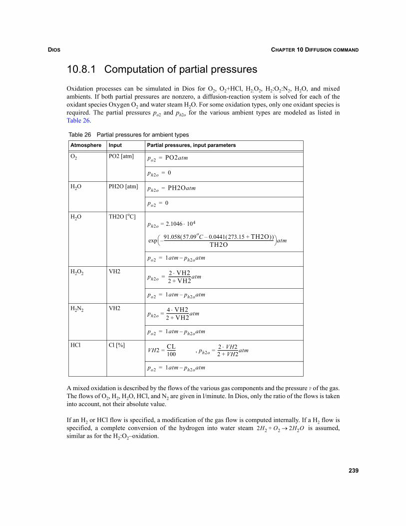
DIOS CHAPTER 10 DIFFUSION COMMAND
10.8.1 Computation of partial pressures
Oxidation processes can be simulated in Dios for O2, O2+HCl, H2:O2, H2:O2:N2, H2O, and mixedambients. If both partial pressures are nonzero, a diffusion-reaction system is solved for each of theoxidant species Oxygen O2 and water steam H2O. For some oxidation types, only one oxidant species isrequired. The partial pressures po2 and ph2o for the various ambient types are modeled as listed inTable 26.
A mixed oxidation is described by the flows of the various gas components and the pressure P of the gas.The flows of O2, H2, H2O, HCl, and N2 are given in l/minute. In Dios, only the ratio of the flows is takeninto account, not their absolute value.
If an H2 or HCl flow is specified, a modification of the gas flow is computed internally. If a H2 flow isspecified, a complete conversion of the hydrogen into water steam is assumed,similar as for the H2:O2–oxidation.
Table 26 Partial pressures for ambient types
Atmosphere Input Partial pressures, input parameters
O2 PO2 [atm]
H2O PH2O [atm]
H2O TH2O [oC]
H2O2 VH2
H2N2 VH2
HCl Cl [%]
po2 PO2atm=
ph2o 0=
ph2o PH2Oatm=
po2 0=
ph2o 2.1046= 104
91.058 57.09 Co 0.0441 273.15 TH2O+( )–( )TH2O
--------------------------------------------------------------------------------------------------------------–⎝ ⎠⎛ ⎞ atmexp
⋅
po2 1atm ph2oatm–=
ph2o2 VH2⋅2 VH2+-----------------------atm=
po2 1atm ph2oatm–=
ph2o4 VH2⋅2 VH2+-----------------------= atm
po2 1atm ph2oatm–=
VH2 CL100--------- , ph2o
2 VH2⋅2 VH2+---------------------= = atm
po2 1atm ph2oatm–=
2H2 O2 2H2O→+
239
DIOSCHAPTER 10 DIFFUSION COMMAND
This reaction reduces the O2 flow, increases the H2O flow and cancels the H2 flow. There must not beany H2 flow left. The modified flows are computed according to:
(301)
A remaining O2 flow is reduced further, if a HCl flow is specified. Formally, this could be described alsoby a complete conversion: 2 HCl + O2→ 2 OH + Cl2. Besides for the modified oxidation rates, thechlorine is neglected in the simulation as for the O2+HCl–oxidation. The modified flows are given as:
(302)
From these (modified) gas flows, the partial pressures are computed according to:
(303)
NOTE The partial pressures are multiplied by the parameter Pressure. If the partial pressure for atleast one of oxygen or water steam is greater than zero, an oxidation process is assumed.Otherwise, an inert diffusion step is simulated. The partial pressures of oxygen and watersteam are used to define the rate constants for the 1D oxidation model and the equilibriumconcentration at the gas interfaces for the 2D oxidant diffusion.
NOTE An inconsistency in the internally used data for HCl oxidations has been removed, therebyestablishing a smooth dependency of the grown oxide thickness on the HCl content. Thechanges affect oxide thicknesses for higher HCl content only, while the data for HCl contentsbelow 5% is not modified.
If the HCl flow exceeds the (remaining or not existing) O2 flow, according to Eq. 302 and Eq. 303, onlythe partial pressure is (slightly) modified; otherwise, the HCl contribution is ignored.
FlowO2FlowO2
0.5FlowH2–:=
FlowH2O FlowH2O FlowH2+:=
FlowH20:=
aa min FlowHCl,2FlowO2( ):=
FlowH2O FlowH2O aa+:=
FlowO2FlowO2
0.5aa–:=
FlowHCl FlowHCl aa–:=
PPi pFlowi
Flowjj∑-----------------------=
240
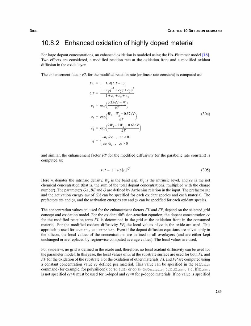
DIOS CHAPTER 10 DIFFUSION COMMAND
10.8.2 Enhanced oxidation of highly doped material
For large dopant concentrations, an enhanced oxidation is modeled using the Ho–Plummer model [18].Two effects are considered, a modified reaction rate at the oxidation front and a modified oxidantdiffusion in the oxide layer.
The enhancement factor FL for the modified reaction rate (or linear rate constant) is computed as:
(304)
and similar, the enhancement factor FP for the modified diffusivity (or the parabolic rate constant) iscomputed as:
(305)
Here ni denotes the intrinsic density, Wg is the band gap, Wi is the intrinsic level, and cc is the netchemical concentration (that is, the sum of the total dopant concentrations, multiplied with the chargenumber). The parameters GA, BE and Q are defined by Arrhenius relation in the input. The prefactor GA0and the activation energy GAW of GA can be specified for each oxidant species and each material. Theprefactors BE0 and Q0, and the activation energies BEW and QW can be specified for each oxidant species.
The concentration values cc, used for the enhancement factors FL and FP, depend on the selected gridconcept and oxidation model. For the oxidant diffusion-reaction equation, the dopant concentration ccfor the modified reaction term FL is determined in the grid at the oxidation front in the consumedmaterial. For the modified oxidant diffusivity FP, the local values of cc in the oxide are used. Thisapproach is used for Newdif=1, SIDIFf=on/off. Even if the dopant diffusion equations are solved only inthe silicon, the local values of the concentrations are defined in all overlayers (and are either keptunchanged or are replaced by regionwise computed average values). The local values are used.
For NewDifF=0, no grid is defined in the oxide and, therefore, no local oxidant diffusivity can be used forthe parameter model. In this case, the local values of cc at the substrate surface are used for both FL andFP for the oxidation of the substrate. For the oxidation of other materials, FL and FP are computed usinga constant concentration value cc defined per material. This value can be specified in the Diffusioncommand (for example, for polysilicon): CC(PO=1e21) or CC(PO(CONCentration=1e21,Element=P)). If Elementis not specified cc>0 must be used for n-doped and cc<0 for p-doped materials. If no value is specified
FL 1 GA CT 1–( )+=
CT1 c1q 1– c2q c3q2+ + +
1 c1 c2 c3+ + +-------------------------------------------------------=
c10.35eV Wi–
kT------------------------------⎝ ⎠
⎛ ⎞exp=
c2Wi Wg 0.57eV+–
kT--------------------------------------------⎝ ⎠
⎛ ⎞exp=
c32Wi 2Wg 0.68eV+–
kT---------------------------------------------------⎝ ⎠
⎛ ⎞exp=
qni cc , cc 0<⁄–
cc ni , cc > 0⁄⎩⎨⎧
=
FP 1 BE cc Q+=
241
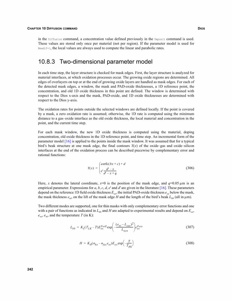
DIOSCHAPTER 10 DIFFUSION COMMAND
in the Diffusion command, a concentration value defined previously in the Deposit command is used.These values are stored only once per material (not per region). If the parameter model is used forNewdif=1, the local values are always used to compute the linear and parabolic rates.
10.8.3 Two-dimensional parameter model
In each time step, the layer structure is checked for mask edges. First, the layer structure is analyzed formaterial interfaces, at which oxidation processes occur. The growing oxide regions are determined. Alledges of overlayers on top or at the end of growing oxide layers are handled as mask edges. For each ofthe detected mask edges, a window, the mask and PAD-oxide thicknesses, a 1D reference point, theconcentration, and old 1D oxide thickness in this point are defined. The window is determined withrespect to the Dios x-axis and the mask, PAD-oxide, and 1D oxide thicknesses are determined withrespect to the Dios y-axis.
The oxidation rates for points outside the selected windows are defined locally. If the point is coveredby a mask, a zero oxidation rate is assumed; otherwise, the 1D rate is computed using the minimumdistance to a gas–oxide interface as the old oxide thickness, the local material and concentration in thepoint, and the current time step.
For each mask window, the new 1D oxide thickness is computed using the material, dopingconcentration, old oxide thickness in the 1D reference point, and time step. An incremental form of theparameter model [16] is applied to the points inside the mask window. It was assumed that for a typicalbird’s beak structure at one mask edge, the final contours Y(x) of the oxide–gas and oxide–siliconinterfaces at the end of the oxidation process can be described piecewise by complementary error andrational functions:
(306)
Here, x denotes the lateral coordinate, x=0 is the position of the mask edge, and q=0.05 μm is anempirical parameter. Expressions for a, b, c, d, e' and d' are given in the literature [16]. These parametersdepend on the reference 1D field oxide thickness Eox, the initial PAD-oxide thickness eox below the mask,the mask thickness eni, on the lift of the mask edge H and the length of the bird’s beak Lbb (all in μm).
Two different modes are supported, one for thin masks with only complementary error functions and onewith a pair of functions as indicated in Lbb and H are adapted to experimental results and depend on Eox,eox, eni, and the temperature T (in K):
(307)
(308)
Y x( )a bx c+( ) d+erfc
e′ d′ x–d′ x– q+----------------------
⎝⎜⎜⎛
=
Lbb KL TLK T–( )EoxPotE
eni Lzae–( )2
Lnen------------------------------–
⎝ ⎠⎜ ⎟⎛ ⎞
eoxPoteexp=
H KH nko nfaceni–( )EoxT
THk---------–⎝ ⎠
⎛ ⎞exp=
242
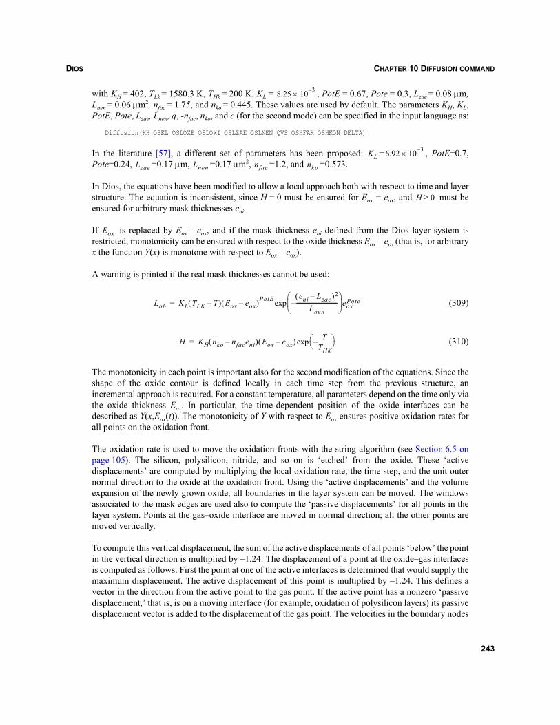
DIOS CHAPTER 10 DIFFUSION COMMAND
with KH = 402, TLk = 1580.3 K, THk = 200 K, KL = , PotE = 0.67, Pote = 0.3, Lzae = 0.08 μm,Lnen = 0.06 μm2, nfac = 1.75, and nko = 0.445. These values are used by default. The parameters KH, KL,PotE, Pote, Lzae, Lnen, q, -nfac, nko, and c (for the second mode) can be specified in the input language as:
Diffusion(KH OSKL OSLOXE OSLOXI OSLZAE OSLNEN QVS OSHFAK OSHKON DELTA)
In the literature [57], a different set of parameters has been proposed: = , PotE=0.7,Pote=0.24, =0.17 μm, =0.17 μm2, =1.2, and =0.573.
In Dios, the equations have been modified to allow a local approach both with respect to time and layerstructure. The equation is inconsistent, since H = 0 must be ensured for Eox = eox, and must beensured for arbitrary mask thicknesses eni.
If is replaced by Eox - eox, and if the mask thickness eni defined from the Dios layer system isrestricted, monotonicity can be ensured with respect to the oxide thickness Eox – eox (that is, for arbitraryx the function Y(x) is monotone with respect to Eox – eox).
A warning is printed if the real mask thicknesses cannot be used:
(309)
(310)
The monotonicity in each point is important also for the second modification of the equations. Since theshape of the oxide contour is defined locally in each time step from the previous structure, anincremental approach is required. For a constant temperature, all parameters depend on the time only viathe oxide thickness Eox. In particular, the time-dependent position of the oxide interfaces can bedescribed as Y(x,Eox(t)). The monotonicity of Y with respect to Eox ensures positive oxidation rates forall points on the oxidation front.
The oxidation rate is used to move the oxidation fronts with the string algorithm (see Section 6.5 onpage 105). The silicon, polysilicon, nitride, and so on is ‘etched’ from the oxide. These ‘activedisplacements’ are computed by multiplying the local oxidation rate, the time step, and the unit outernormal direction to the oxide at the oxidation front. Using the ‘active displacements’ and the volumeexpansion of the newly grown oxide, all boundaries in the layer system can be moved. The windowsassociated to the mask edges are used also to compute the ‘passive displacements’ for all points in thelayer system. Points at the gas–oxide interface are moved in normal direction; all the other points aremoved vertically.
To compute this vertical displacement, the sum of the active displacements of all points ‘below’ the pointin the vertical direction is multiplied by –1.24. The displacement of a point at the oxide–gas interfacesis computed as follows: First the point at one of the active interfaces is determined that would supply themaximum displacement. The active displacement of this point is multiplied by –1.24. This defines avector in the direction from the active point to the gas point. If the active point has a nonzero ‘passivedisplacement,’ that is, is on a moving interface (for example, oxidation of polysilicon layers) its passivedisplacement vector is added to the displacement of the gas point. The velocities in the boundary nodes
8.25 10 3–×
KL 6.92 10 3–×Lzae Lnen nfac nko
H 0≥
Eox
Lbb KL TLK T–( ) Eox eox–( )PotE eni Lzae–( )2
Lnen------------------------------–
⎝ ⎠⎜ ⎟⎛ ⎞
eoxPoteexp=
H KH nko nfaceni–( ) Eox eox–( ) TTHk---------–⎝ ⎠
⎛ ⎞exp=
243
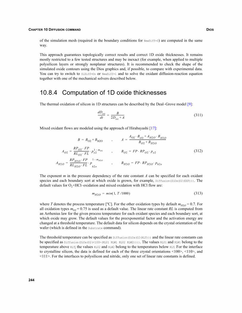
DIOSCHAPTER 10 DIFFUSION COMMAND
of the simulation mesh (required in the boundary conditions for NewDiff=0) are computed in the sameway.
This approach guarantees topologically correct results and correct 1D oxide thicknesses. It remainsmostly restricted to a few tested structures and may be inexact (for example, when applied to multiplepolysilicon layers or strongly nonplanar structures). It is recommended to check the shape of thesimulated oxide contours using the Dios graphics and, if possible, to compare with experimental data.You can try to switch to SiDiff=On or NewDiff=1 and to solve the oxidant diffusion-reaction equationtogether with one of the mechanical solvers described below.
10.8.4 Computation of 1D oxide thicknesses
The thermal oxidation of silicon in 1D structures can be described by the Deal–Grove model [9]:
(311)
Mixed oxidant flows are modeled using the approach of Hirabayashi [17]:
(312)
The exponent m in the pressure dependency of the rate constant A can be specified for each oxidantspecies and each boundary sort at which oxide is grown, for example, Diffusion(SiOx(O2(EXP))). Thedefault values for O2+HCl–oxidation and mixed oxidation with HCl flow are:
(313)
where T denotes the process temperature [oC]. For the other oxidation types by default mH2O = 0.7. Forall oxidation types mO2 = 0.75 is used as a default value. The linear rate constant RL is computed froman Arrhenius law for the given process temperature for each oxidant species and each boundary sort, atwhich oxide may grow. The default values for the preexponential factor and the activation energy arechanged at a threshold temperature. The default data for silicon depends on the crystal orientation of thewafer (which is defined in the Substrate command).
The threshold temperature can be specified as Diffusion(SiOx(O2(RLT))) and the linear rate constants canbe specified as Diffusion(SiOx(O2(<100>(RL01 RLW1 RL02 RLW2)))). The values RL01 and RLW1 belong to thetemperature above RLT; the values RL02 and RLW2 belong to the temperatures below RLT. For the interfaceto crystalline silicon, the data is defined for each of the three crystal orientations <100>, <110>, and<111>. For the interfaces to polysilicon and nitride, only one set of linear rate constants is defined.
dDoxdt
------------ B2Dox A+----------------------=
B BO2 BH2O+= , AAO2 B⋅ O2 AH2O B⋅ H2O+
BO2 BH2O+--------------------------------------------------------------=
AO2RPO2 FP⋅RLO2 FL⋅-------------------------- po2
1 mO2–⋅= , BO2 FP RPO2 po2⋅ ⋅=
AH2ORPH2O FP⋅RLH2O FL⋅----------------------------- p⋅
h2o
1 mH2O–= , BH2O FP RPH2O ph2o⋅ ⋅=
mH2O min 1 T 1000⁄,( )=
244
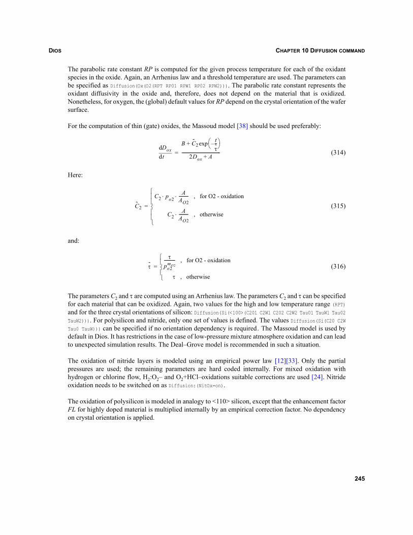
DIOS CHAPTER 10 DIFFUSION COMMAND
The parabolic rate constant RP is computed for the given process temperature for each of the oxidantspecies in the oxide. Again, an Arrhenius law and a threshold temperature are used. The parameters canbe specified as Diffusion(Ox(O2(RPT RP01 RPW1 RP02 RPW2))). The parabolic rate constant represents theoxidant diffusivity in the oxide and, therefore, does not depend on the material that is oxidized.Nonetheless, for oxygen, the (global) default values for RP depend on the crystal orientation of the wafersurface.
For the computation of thin (gate) oxides, the Massoud model [38] should be used preferably:
(314)
Here:
(315)
and:
(316)
The parameters C2 and τ are computed using an Arrhenius law. The parameters C2 and τ can be specifiedfor each material that can be oxidized. Again, two values for the high and low temperature range (RPT)and for the three crystal orientations of silicon: Diffusion(Si(<100>(C201 C2W1 C202 C2W2 Tau01 TauW1 Tau02TauW2))). For polysilicon and nitride, only one set of values is defined. The values Diffusion(Si(C20 C2WTau0 TauW))) can be specified if no orientation dependency is required. The Massoud model is used bydefault in Dios. It has restrictions in the case of low-pressure mixture atmosphere oxidation and can leadto unexpected simulation results. The Deal–Grove model is recommended in such a situation.
The oxidation of nitride layers is modeled using an empirical power law [12][33]. Only the partialpressures are used; the remaining parameters are hard coded internally. For mixed oxidation withhydrogen or chlorine flow, H2:O2– and O2+HCl–oxidations suitable corrections are used [24]. Nitrideoxidation needs to be switched on as Diffusion:(NitOx=on).
The oxidation of polysilicon is modeled in analogy to <110> silicon, except that the enhancement factorFL for highly doped material is multiplied internally by an empirical correction factor. No dependencyon crystal orientation is applied.
tddDox
B C2tτ--–⎝ ⎠
⎛ ⎞exp+
2Dox A+--------------------------------------=
C2
C2 p⋅ o2A
AO2---------⋅ , for O2 - oxidation
C2A
AO2---------⋅ , otherwise
⎩⎪⎪⎨⎪⎪⎧
=
τ
τpo2
mO2----------- , for O2 - oxidation
τ , otherwise⎩⎪⎨⎪⎧
=
245
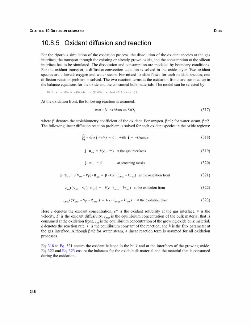
DIOSCHAPTER 10 DIFFUSION COMMAND
10.8.5 Oxidant diffusion and reaction
For the rigorous simulation of the oxidation process, the dissolution of the oxidant species at the gasinterface, the transport through the existing or already grown oxide, and the consumption at the siliconinterface has to be simulated. The dissolution and consumption are modeled by boundary conditions.For the oxidant transport, a diffusion-convection equation is solved in the oxide layer. Two oxidantspecies are allowed: oxygen and water steam. For mixed oxidant flows for each oxidant species, onediffusion-reaction problem is solved. The two reaction terms at the oxidation fronts are summed up inthe balance equations for the oxide and the consumed bulk materials. The model can be selected by:
Diffusion:(Models(Oxidation(ModDifOxidant=Diffusion)))
At the oxidation front, the following reaction is assumed:
(317)
where β denotes the stoichiometry coefficient of the oxidant. For oxygen, β=1; for water steam, β=2.The following linear diffusion reaction problem is solved for each oxidant species in the oxide regions:
(318)
(319)
(320)
(321)
(322)
(323)
Here c denotes the oxidant concentration, c* is the oxidant solubility at the gas interface, v is thevelocity, D is the oxidant diffusivity, cmat is the equilibrium concentration of the bulk material that isconsumed at the oxidation front, cox is the equilibrium concentration of the growing oxide bulk material,k denotes the reaction rate, is the equilibrium constant of the reaction, and h is the flux parameter atthe gas interface. Although β=2 for water steam, a linear reaction term is assumed for all oxidationprocesses.
Eq. 318 to Eq. 321 ensure the oxidant balance in the bulk and at the interfaces of the growing oxide.Eq. 322 and Eq. 323 ensure the balances for the oxide bulk material and the material that is consumedduring the oxidation.
mat β oxidant⋅+ SiO2⇔
t∂∂c j cv+( )div+ 0 , with j D cgrad–= =
j n⋅ ox h c c∗–( ) at the gas interfaces=
j n⋅ ox 0 at screening masks=
j n⋅ ox c vox vΓ–( ) n⋅ ox+ β k c cmat⋅ kcox–( ) at the oxidation front⋅=
cox vox vΓ–( ) nox⋅( ) k c cmat⋅ kcox–( ) at the oxidation front–=
cmat vmat vΓ–( ) nmat⋅( ) k c cmat⋅ kcox–( ) at the oxidation front=
k
246
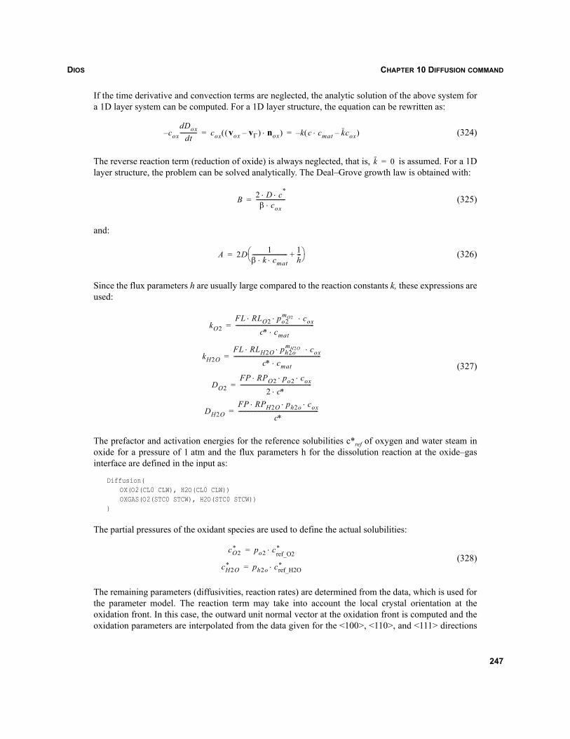
DIOS CHAPTER 10 DIFFUSION COMMAND
If the time derivative and convection terms are neglected, the analytic solution of the above system fora 1D layer system can be computed. For a 1D layer structure, the equation can be rewritten as:
(324)
The reverse reaction term (reduction of oxide) is always neglected, that is, is assumed. For a 1Dlayer structure, the problem can be solved analytically. The Deal–Grove growth law is obtained with:
(325)
and:
(326)
Since the flux parameters h are usually large compared to the reaction constants k, these expressions areused:
(327)
The prefactor and activation energies for the reference solubilities c*ref of oxygen and water steam inoxide for a pressure of 1 atm and the flux parameters h for the dissolution reaction at the oxide–gasinterface are defined in the input as:
Diffusion(OX(O2(CL0 CLW), H2O(CL0 CLW))OXGAS(O2(STC0 STCW), H2O(STC0 STCW))
)
The partial pressures of the oxidant species are used to define the actual solubilities:
(328)
The remaining parameters (diffusivities, reaction rates) are determined from the data, which is used forthe parameter model. The reaction term may take into account the local crystal orientation at theoxidation front. In this case, the outward unit normal vector at the oxidation front is computed and theoxidation parameters are interpolated from the data given for the <100>, <110>, and <111> directions
coxdDox
dt------------– cox vox vΓ–( ) nox⋅( ) k c c⋅ mat kcox–( )–= =
k 0=
B 2 D c*⋅ ⋅β cox⋅
---------------------=
A 2D 1β k cmat⋅ ⋅------------------------- 1
h---+⎝ ⎠
⎛ ⎞=
kO2FL RLO2 po2
mO2 cox⋅ ⋅ ⋅
c∗ cmat⋅--------------------------------------------------------=
kH2OFL RLH2O ph2o
mH2O cox⋅ ⋅ ⋅
c∗ cmat⋅--------------------------------------------------------------=
DO2FP RPO2 po2 cox⋅ ⋅ ⋅
2 c∗⋅---------------------------------------------------=
DH2OFP RPH2O ph2o cox⋅ ⋅ ⋅
c∗---------------------------------------------------------=
cO2* po2 c⋅ ref_O2
*=
cH2O* ph2o cref_H2O
*⋅=
247
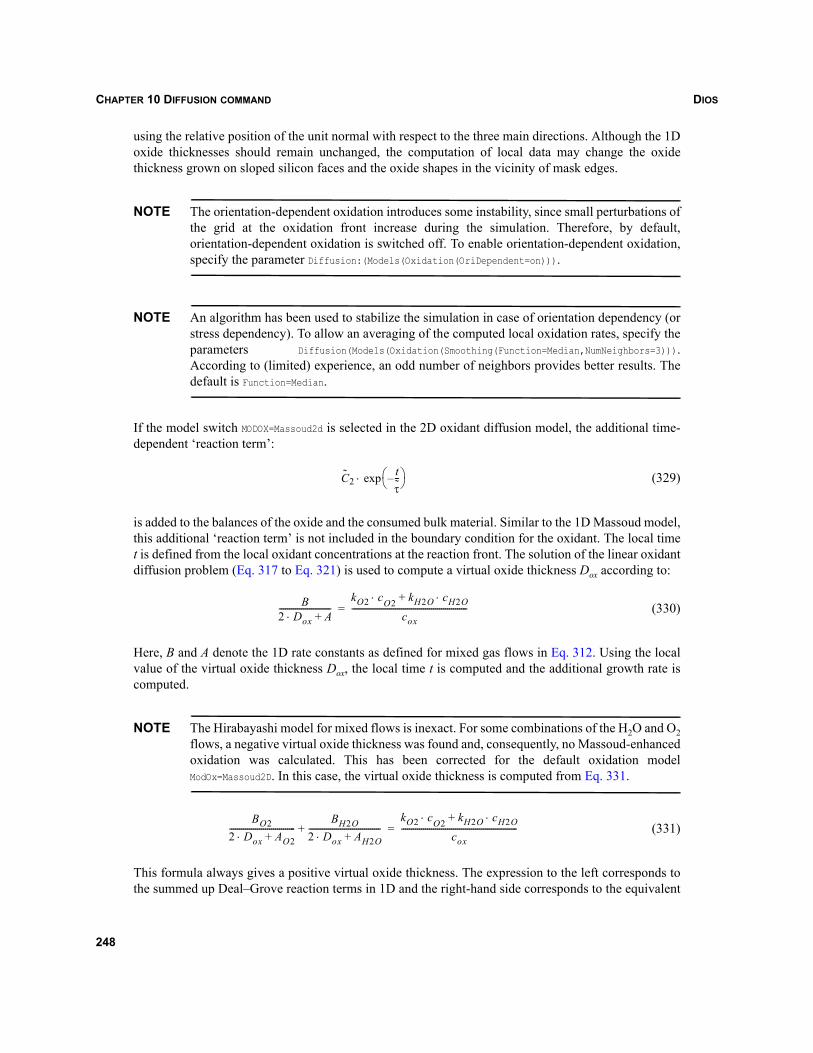
DIOSCHAPTER 10 DIFFUSION COMMAND
using the relative position of the unit normal with respect to the three main directions. Although the 1Doxide thicknesses should remain unchanged, the computation of local data may change the oxidethickness grown on sloped silicon faces and the oxide shapes in the vicinity of mask edges.
NOTE The orientation-dependent oxidation introduces some instability, since small perturbations ofthe grid at the oxidation front increase during the simulation. Therefore, by default,orientation-dependent oxidation is switched off. To enable orientation-dependent oxidation,specify the parameter Diffusion:(Models(Oxidation(OriDependent=on))).
NOTE An algorithm has been used to stabilize the simulation in case of orientation dependency (orstress dependency). To allow an averaging of the computed local oxidation rates, specify theparameters Diffusion(Models(Oxidation(Smoothing(Function=Median,NumNeighbors=3))).According to (limited) experience, an odd number of neighbors provides better results. Thedefault is Function=Median.
If the model switch MODOX=Massoud2d is selected in the 2D oxidant diffusion model, the additional time-dependent ‘reaction term’:
(329)
is added to the balances of the oxide and the consumed bulk material. Similar to the 1D Massoud model,this additional ‘reaction term’ is not included in the boundary condition for the oxidant. The local timet is defined from the local oxidant concentrations at the reaction front. The solution of the linear oxidantdiffusion problem (Eq. 317 to Eq. 321) is used to compute a virtual oxide thickness Dox according to:
(330)
Here, B and A denote the 1D rate constants as defined for mixed gas flows in Eq. 312. Using the localvalue of the virtual oxide thickness Dox, the local time t is computed and the additional growth rate iscomputed.
NOTE The Hirabayashi model for mixed flows is inexact. For some combinations of the H2O and O2flows, a negative virtual oxide thickness was found and, consequently, no Massoud-enhancedoxidation was calculated. This has been corrected for the default oxidation modelModOx=Massoud2D. In this case, the virtual oxide thickness is computed from Eq. 331.
(331)
This formula always gives a positive virtual oxide thickness. The expression to the left corresponds tothe summed up Deal–Grove reaction terms in 1D and the right-hand side corresponds to the equivalent
C2tτ--–⎝ ⎠
⎛ ⎞exp⋅
B2 D⋅ ox A+--------------------------
kO2 c⋅ O2 kH2O cH2O⋅+cox
----------------------------------------------------------=
BO22 D⋅ ox AO2+---------------------------------
BH2O2 D⋅ ox AH2O+------------------------------------+
kO2 c⋅ O2 kH2O cH2O⋅+cox
----------------------------------------------------------=
248
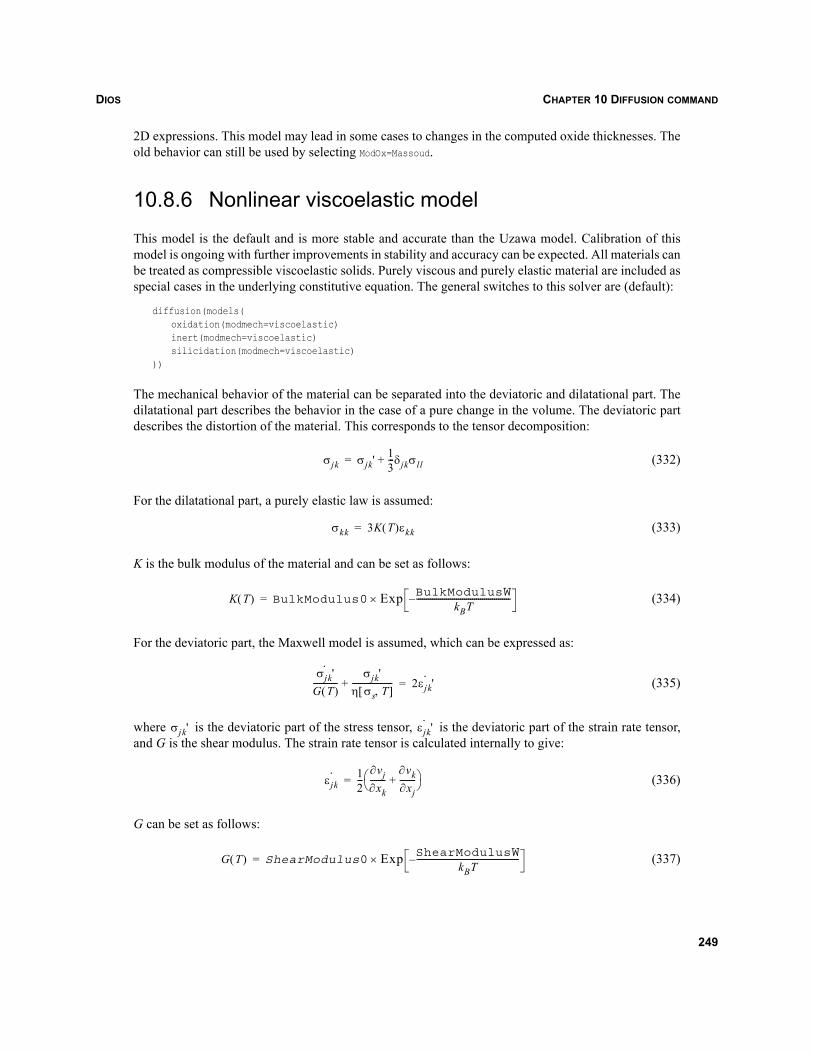
DIOS CHAPTER 10 DIFFUSION COMMAND
2D expressions. This model may lead in some cases to changes in the computed oxide thicknesses. Theold behavior can still be used by selecting ModOx=Massoud.
10.8.6 Nonlinear viscoelastic model
This model is the default and is more stable and accurate than the Uzawa model. Calibration of thismodel is ongoing with further improvements in stability and accuracy can be expected. All materials canbe treated as compressible viscoelastic solids. Purely viscous and purely elastic material are included asspecial cases in the underlying constitutive equation. The general switches to this solver are (default):
diffusion(models(oxidation(modmech=viscoelastic)inert(modmech=viscoelastic)silicidation(modmech=viscoelastic)
))
The mechanical behavior of the material can be separated into the deviatoric and dilatational part. Thedilatational part describes the behavior in the case of a pure change in the volume. The deviatoric partdescribes the distortion of the material. This corresponds to the tensor decomposition:
(332)
For the dilatational part, a purely elastic law is assumed:
(333)
K is the bulk modulus of the material and can be set as follows:
(334)
For the deviatoric part, the Maxwell model is assumed, which can be expressed as:
(335)
where is the deviatoric part of the stress tensor, is the deviatoric part of the strain rate tensor,and G is the shear modulus. The strain rate tensor is calculated internally to give:
(336)
G can be set as follows:
(337)
σjk σjk'13---δjkσll+=
σkk 3K T( )εkk=
K T( ) BulkModulus0 Exp BulkModulusWkBT
-----------------------------------------------–×=
σjk'·
G T( )------------
σjk'η σs T,[ ]--------------------+ 2εjk'
·=
σjk' εjk'·
εjk· 1
2---
∂vj∂xk--------
∂vk∂xj--------+⎝ ⎠
⎛ ⎞=
G T( ) ShearModulus0 Exp ShearModulusWkBT
---------------------------------------------------–×=
249
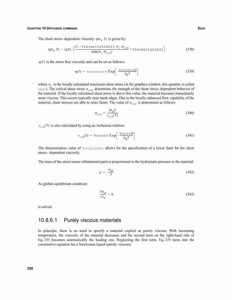
DIOSCHAPTER 10 DIFFUSION COMMAND
The shear stress–dependent viscosity is given by:
(338)
is the stress free viscosity and can be set as follows:
(339)
where is the locally calculated maximum shear stress (in the graphics window, this quantity is calledshear). The critical shear stress determines the strength of the shear stress–dependent behavior ofthe material. If the locally calculated shear stress is above this value, the material becomes immediatelymore viscous. This occurs typically near mask edges. Due to the locally enhanced flow capability of thematerial, shear stresses are able to relax faster. The value of is determined as follows:
(340)
is also calculated by using an Arrhenius relation:
(341)
The dimensionless value of ViscosityLimit allows for the specification of a lower limit for the shearstress– dependent viscosity.
The trace of the stress tensor (dilatational part) is proportional to the hydrostatic pressure in the material:
(342)
As global equilibrium condition:
(343)
is solved.
10.8.6.1 Purely viscous materials
In principle, there is no need to specify a material explicit as purely viscous. With increasingtemperature, the viscosity of the material decreases and the second term on the right-hand side ofEq. 335 becomes automatically the leading one. Neglecting the first term, Eq. 335 turns into theconstitutive equation for a Newtonian liquid (purely viscous).
η σs T,( )
η σs T,( ) η T( )1 Vis ityLimitcos–( ) σ⋅ s σcrit⁄
σs σcrit⁄( )sinh---------------------------------------------------------------------------------------------- Vis ityLimitcos+⎝ ⎠
⎛ ⎞⋅=
η T( )
η T( ) Viscosity0 Exp ViscosityWkBT
--------------------------------–×=
σsσcrit
σcrit
σcrit2kBT
vcrit T( )-------------------=
vcrit T( )
vcrit T( ) Vcrit0 Exp VcritWkBT
-----------------------–×=
pσkk3
--------–=
∂σjk∂xk---------- 0=
250
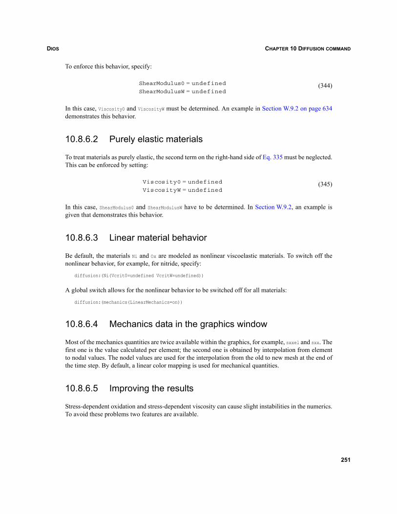
DIOS CHAPTER 10 DIFFUSION COMMAND
To enforce this behavior, specify:
(344)
In this case, Viscosity0 and ViscosityW must be determined. An example in Section W.9.2 on page 634demonstrates this behavior.
10.8.6.2 Purely elastic materials
To treat materials as purely elastic, the second term on the right-hand side of Eq. 335 must be neglected.This can be enforced by setting:
(345)
In this case, ShearModulus0 and ShearModulusW have to be determined. In Section W.9.2, an example isgiven that demonstrates this behavior.
10.8.6.3 Linear material behavior
Be default, the materials Ni and Ox are modeled as nonlinear viscoelastic materials. To switch off thenonlinear behavior, for example, for nitride, specify:
diffusion:(Ni(Vcrit0=undefined VcritW=undefined))
A global switch allows for the nonlinear behavior to be switched off for all materials:
diffusion:(mechanics(LinearMechanics=on))
10.8.6.4 Mechanics data in the graphics window
Most of the mechanics quantities are twice available within the graphics, for example, sxxel and sxx. Thefirst one is the value calculated per element; the second one is obtained by interpolation from elementto nodal values. The nodel values are used for the interpolation from the old to new mesh at the end ofthe time step. By default, a linear color mapping is used for mechanical quantities.
10.8.6.5 Improving the results
Stress-dependent oxidation and stress-dependent viscosity can cause slight instabilities in the numerics.To avoid these problems two features are available.
ShearModulus0 undefined=ShearModulusW undefined=
Vis ity0cos undefined=Vis ityWcos undefined=
251
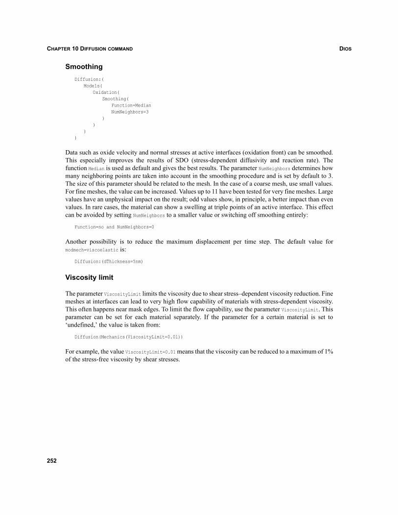
DIOSCHAPTER 10 DIFFUSION COMMAND
SmoothingDiffusion:(
Models(Oxidation(
Smoothing(Function=MedianNumNeighbors=3
))
))
Data such as oxide velocity and normal stresses at active interfaces (oxidation front) can be smoothed.This especially improves the results of SDO (stress-dependent diffusivity and reaction rate). Thefunction Median is used as default and gives the best results. The parameter NumNeighbors determines howmany neighboring points are taken into account in the smoothing procedure and is set by default to 3.The size of this parameter should be related to the mesh. In the case of a coarse mesh, use small values.For fine meshes, the value can be increased. Values up to 11 have been tested for very fine meshes. Largevalues have an unphysical impact on the result; odd values show, in principle, a better impact than evenvalues. In rare cases, the material can show a swelling at triple points of an active interface. This effectcan be avoided by setting NumNeighbors to a smaller value or switching off smoothing entirely:
Function=no and NumNeighbors=0
Another possibility is to reduce the maximum displacement per time step. The default value formodmech=viscoelastic is:
Diffusion:(dThickness=5nm)
Viscosity limit
The parameter ViscosityLimit limits the viscosity due to shear stress–dependent viscosity reduction. Finemeshes at interfaces can lead to very high flow capability of materials with stress-dependent viscosity.This often happens near mask edges. To limit the flow capability, use the parameter ViscosityLimit. Thisparameter can be set for each material separately. If the parameter for a certain material is set to‘undefined,’ the value is taken from:
Diffusion(Mechanics(ViscosityLimit=0.01))
For example, the value ViscosityLimit=0.01 means that the viscosity can be reduced to a maximum of 1%of the stress-free viscosity by shear stresses.
252
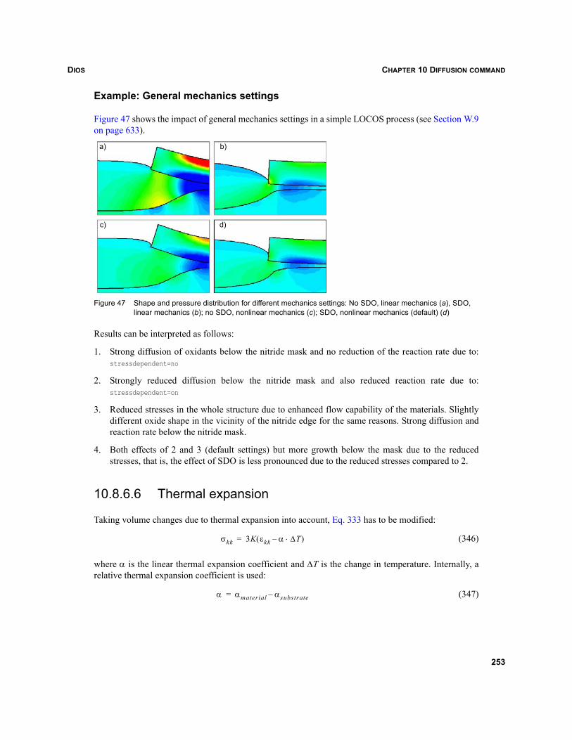
DIOS CHAPTER 10 DIFFUSION COMMAND
Example: General mechanics settings
Figure 47 shows the impact of general mechanics settings in a simple LOCOS process (see Section W.9on page 633).
Figure 47 Shape and pressure distribution for different mechanics settings: No SDO, linear mechanics (a), SDO, linear mechanics (b); no SDO, nonlinear mechanics (c); SDO, nonlinear mechanics (default) (d)
Results can be interpreted as follows:
1. Strong diffusion of oxidants below the nitride mask and no reduction of the reaction rate due to:stressdependent=no
2. Strongly reduced diffusion below the nitride mask and also reduced reaction rate due to:stressdependent=on
3. Reduced stresses in the whole structure due to enhanced flow capability of the materials. Slightlydifferent oxide shape in the vicinity of the nitride edge for the same reasons. Strong diffusion andreaction rate below the nitride mask.
4. Both effects of 2 and 3 (default settings) but more growth below the mask due to the reducedstresses, that is, the effect of SDO is less pronounced due to the reduced stresses compared to 2.
10.8.6.6 Thermal expansion
Taking volume changes due to thermal expansion into account, Eq. 333 has to be modified:
(346)
where α is the linear thermal expansion coefficient and ΔT is the change in temperature. Internally, arelative thermal expansion coefficient is used:
(347)
a) b)
c) d)
σkk 3K εkk α ΔT⋅–( )=
α αmaterial αsubstrate–=
253
DIOSCHAPTER 10 DIFFUSION COMMAND
This means that the substrate can expand freely and the layers above are forced to follow the motion ofthe substrate due to thermal expansion. To specify a thermal expansion coefficient, for example, for Ox( ):
Diffusion(Ox(Expansion=...))
An example is given in Section W.9.4 on page 635.
10.8.6.7 Initial film stress
To model initial film stresses in deposited films, for example, nitride, stresses, pressure or density canbe prescribed in the Deposit command, for example:
Deposit(InitialValue(sxx=... szz=...)
After deposition, these quantities are prescribed homogeneously over the whole deposited layer. Thissituation usually does not correspond to a mechanical equilibrium state. A subsequent Diffusioncommand forces the mechanics solver to work and the system immediately goes into a equilibrium state.To model this, set:
Diffusion(Mechanics(AlwaysMechanics=on))
If stresses in the substrate are also of interest:
Diffusion(Mechanics(FullMechanics=on))
must be set additionally. This is demonstrated by an example in Section W.9.3 on page 635.
10.8.6.8 Stress-dependent oxidation (SDO)
During oxidation, the reaction rate and diffusivity of the oxidant can be affected by mechanicalquantities in the following way:
(348)
(349)
where is the normal stress acting onto the specific interface and is stress-free reaction rate. Theparameter VK is defined at interfaces where oxidation can occur, p is the hydrostatic pressure in oxide,and VD is defined in oxide for H2O and O2. For example:
diffusion(ox(H2O(VD=... )))diffusion(oxpo(O2(VK=... )))
αOx
k σn T,( ) k0 min 1σnVK
kBT--------------
⎝ ⎠⎜ ⎟⎛ ⎞
exp,⎝ ⎠⎜ ⎟⎛ ⎞
⎝ ⎠⎜ ⎟⎛ ⎞
=
Dod σkk T,( ) D0 min 1 pVDkBT-----------–⎝ ⎠
⎛ ⎞exp,⎝ ⎠⎛ ⎞
⎝ ⎠⎛ ⎞=
σn k0
254
DIOS CHAPTER 10 DIFFUSION COMMAND
10.8.7 Additional mechanic models
10.8.7.1 Linear viscoelastic mechanical equations
The linear viscoelastic model is the simplest numeric model to account for the mechanical deformationof the layer structure during an oxidation. One limitation of the model is that nonlinear coupling betweenstress computation and oxidant diffusion/reaction cannot be simulated. In order to handle standard fieldoxidation and polyoxidation processes, the mechanics solver described in this section can be combinedwith the parameter model to compute the correct oxidation rates in the vicinity of the mask edges.
No global stress free reference state is assumed for the oxide, but the reference state is defined locally.For any point x, you can cut out a neighborhood δ and allow it to relax. The locally defined deformationis related in the usual way to a deformation tensor in the selected neighborhood. The deformationtensor in any point x is defined as the limit for δ → 0:
(350)
There is no global integrability condition for this locally defined deformation tensor. Furthermore, notalways a time evolution according to:
(351)
can be assumed. This equation can be assumed only if the material ‘remembers’ its initial state and triesto return into this state, that is, for elastic materials. If the stresses relax in a certain time after a flow, thematerial cannot ‘remember’ its initial state. The neighborhood will no longer expand. By definition,
. The oxide flow leads to a reduction of εl. The simplest equation for this behavior is:
(352)
For a linear relation between stress and deformation tensor:
(353)
the following evolution equation for the stress is obtained:
(354)
that is, a viscoelastic material law. The is used as the state variable. E and λ are tensors, whichhave in the isotropic case two independent components: one describing the volume change and onedescribing pure shear for fixed volume.
εδl
εl x( ) εδl x( )
δ 0→lim=
t∂∂εij
xi∂∂vj
xj∂∂vi+=
εl 0=
t∂∂εij λεij+ xi∂
∂vjxj∂
∂vi+=
σ Eεl=
t∂∂σi j λσij+ E xi∂
∂vjxj∂
∂vi+⎝ ⎠⎜ ⎟⎛ ⎞
=
εl 2 2×
255
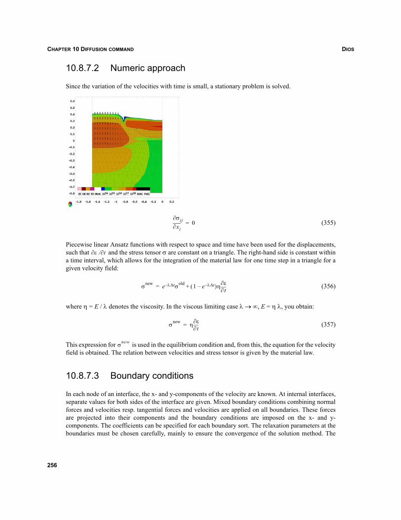
DIOSCHAPTER 10 DIFFUSION COMMAND
10.8.7.2 Numeric approach
Since the variation of the velocities with time is small, a stationary problem is solved.
(355)
Piecewise linear Ansatz functions with respect to space and time have been used for the displacements,such that and the stress tensor σ are constant on a triangle. The right-hand side is constant withina time interval, which allows for the integration of the material law for one time step in a triangle for agiven velocity field:
(356)
where η = E / λ denotes the viscosity. In the viscous limiting case λ → ∞, E = η λ, you obtain:
(357)
This expression for is used in the equilibrium condition and, from this, the equation for the velocityfield is obtained. The relation between velocities and stress tensor is given by the material law.
10.8.7.3 Boundary conditions
In each node of an interface, the x- and y-components of the velocity are known. At internal interfaces,separate values for both sides of the interface are given. Mixed boundary conditions combining normalforces and velocities resp. tangential forces and velocities are applied on all boundaries. These forcesare projected into their components and the boundary conditions are imposed on the x- and y-components. The coefficients can be specified for each boundary sort. The relaxation parameters at theboundaries must be chosen carefully, mainly to ensure the convergence of the solution method. The
xi∂∂σi j 0=
ε∂ t∂⁄
σnew e λ tΔ– σold 1 e λ tΔ––( )ηt∂
∂ε+=
σnew η t∂∂ε=
σnew
256
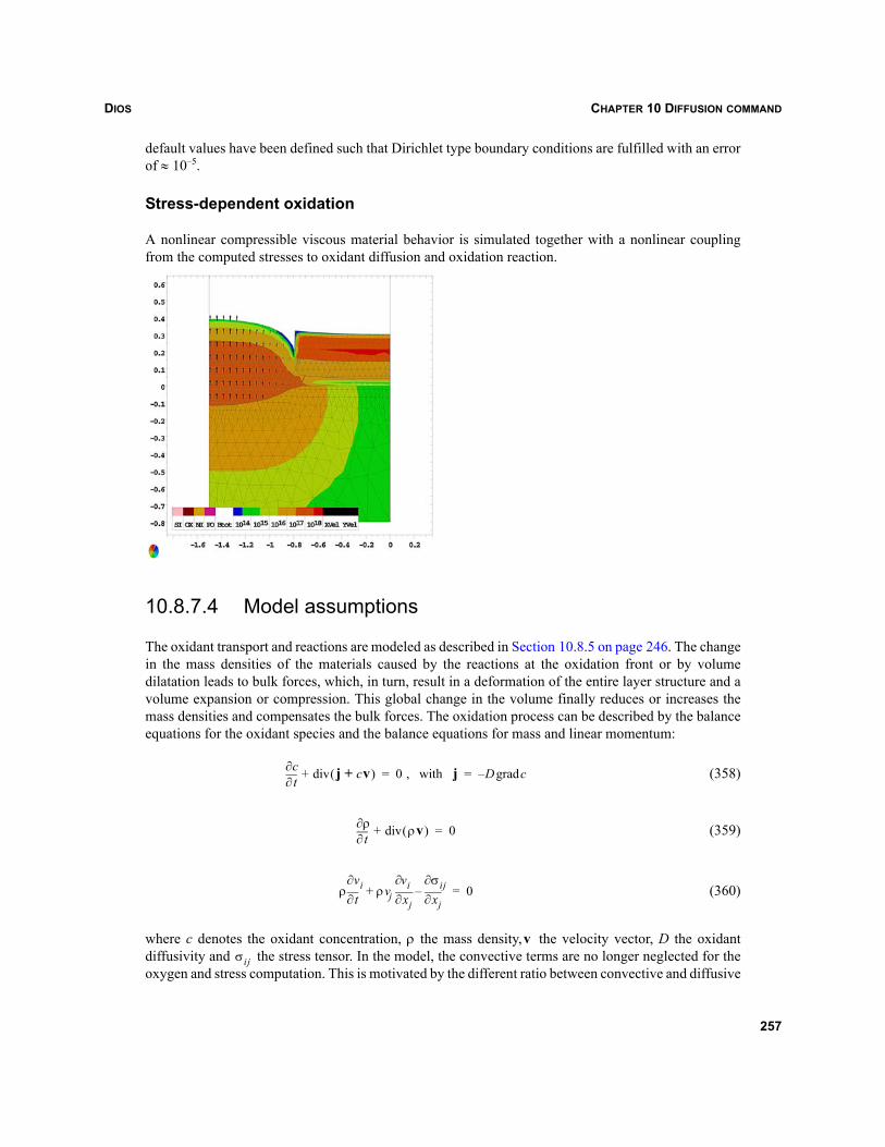
DIOS CHAPTER 10 DIFFUSION COMMAND
default values have been defined such that Dirichlet type boundary conditions are fulfilled with an errorof ≈ 10–5.
Stress-dependent oxidation
A nonlinear compressible viscous material behavior is simulated together with a nonlinear couplingfrom the computed stresses to oxidant diffusion and oxidation reaction.
10.8.7.4 Model assumptions
The oxidant transport and reactions are modeled as described in Section 10.8.5 on page 246. The changein the mass densities of the materials caused by the reactions at the oxidation front or by volumedilatation leads to bulk forces, which, in turn, result in a deformation of the entire layer structure and avolume expansion or compression. This global change in the volume finally reduces or increases themass densities and compensates the bulk forces. The oxidation process can be described by the balanceequations for the oxidant species and the balance equations for mass and linear momentum:
(358)
(359)
(360)
where c denotes the oxidant concentration, ρ the mass density, the velocity vector, D the oxidantdiffusivity and the stress tensor. In the model, the convective terms are no longer neglected for theoxygen and stress computation. This is motivated by the different ratio between convective and diffusive
t∂∂c j cv+( )div+ 0 , with j D cgrad–= =
t∂∂ρ ρv( )div+ 0=
ρ t∂∂vi ρvj xj∂
∂vixj∂
∂σij–+ 0=
vσi j
257
DIOSCHAPTER 10 DIFFUSION COMMAND
oxidant transport in the different parts of a 2D structure. Usually for a 1D simulation, a coordinatetransformation can be applied, as in the Deal–Grove model [15][19]. After the coordinatetransformation, no convection flux is left in the oxidant diffusion equations. In 2D structures, such acoordinate transformation cannot be applied and convective transport has to be accounted for. In thenonlinear model, the time derivatives and convection terms are both included. By default, the convectiveterms are handled in Dios in an extra convection step, as described in Section 10.4 on page 222 for thedopant transport. Eq. 358 to Eq. 360 are solved if one of the modelsDiffusion(Mechanics(Solver=Uzawa|Viscous|Extrapolation)) is selected.
10.8.7.5 Material law
By default, a purely viscous material law is used for all materials:
(361)
A scalar weight factor Diffusion(SI(Viscous)) (default, 1), a relaxation time Diffusion(SI(Elastic0)(default, 0) and its activation energy ElasticW (default, 0) can be specified to model a viscoelasticmaterial law:
(362)
For the viscoelastic model, the default value of Diffusion(SI(Elastic0=0.1)) is used. A nonlinear relationbetween both viscosities μ and λ and the stress can be assumed, as suggested in [45]:
(363)
(364)
(365)
where S denotes the maximum shear stress (that is, the largest eigenvalue of the stress tensor). Thecharacteristic volume is a model fit parameter. The ratios:
(366)
stabilize the numeric algorithm. The parameters can be specified as:
DIFFusion(MyMin/Myref=1.E-3,MyMax/MyRef=1)
σi j pδi j– λ vδi jdiv μxj∂
∂vixi∂
∂vj+⎝ ⎠⎜ ⎟⎛ ⎞
+ +=
Elastic σ· ij Viscous σi j+ λ vδijdiv μ xj∂∂vi
xi∂∂vj+
⎝ ⎠⎜ ⎟⎛ ⎞
+=
μ μ0minμmaxμref------------ max
μminμref----------- x
xsinh-------------,⎝ ⎠
⎛ ⎞,⎝ ⎠⎛ ⎞=
λ λ0minμmaxμref------------ max
μminμref----------- x
xsinh-------------,⎝ ⎠
⎛ ⎞,⎝ ⎠⎛ ⎞=
with xSVμ2kT---------=
Vμ
μminμref-----------
μmaxμref------------,
258
DIOS CHAPTER 10 DIFFUSION COMMAND
Uzawa model
The materials can be assumed to be perfectly incompressible. In this case, equation is replaced by:
(367)
Equations are solved if the parameter DIFFusion(Mechanics(Solver=Uzawa)) is specified. The Uzawaalgorithm is a well known iterative scheme for the approximate solution of the incompressible creepingflow problem. In Dios, the linear momentum balance equation is solved, but instead of solving the massbalance equation, pressure increments are computed from:
(368)
The iteration is stopped if both the pressure increments and velocity increments are small enough. TheUzawa iteration scheme is known to be slowly convergent. For time-saving reasons, in Dios, the matrixis factorized only once and the termination conditions have been chosen to be relatively weak. Theparameter λ can be specified as LAMfac. The default value of LAMfac for the Uzawa scheme is 0.6. It isrecommended to check the resulting divergence on the grid using the Dios graphics or by printing theextremal values.
Viscous model
For Solver=Viscous, equations are solved. Since in this model, the material is assumed to be compressible,the relation between the pressure p and mass density ρ must be given by a material law:
(369)
where ρ0 denotes the equilibrium density for the material. The parameter OZP1 determines the force(pressure) that is developed in the material for compression or expansion. The default values are chosensuch that nearly no variation in the density of a material is obtained. To stabilize the numeric algorithm,the density–pressure relation has been modified internally:
(370)
This modification should not affect the normal behavior of the model, but should prevent extremalpressure values. The parameters can be specified as:
DIFFusion(OZP0=1atm,OZP1=1e7atm)
For Solver=Viscous, thermal expansion of the materials can be simulated. Nonzero thermal expansioncoefficients Diffusion(SI(Expansion=.../K)) must be prescribed.
Reference temperatures Diffusion(Si(ExpansionRefTemp=...)) can also be prescribed per material. In thiscase, the reference density is chosen according to the current and the reference temperature:
(371)
vdiv 0=
pi 1+ pi λ vdiv+=
p OZP0 OZP1ρ ρ0–
ρ0---------------+=
p OZP0 OZP1ρ ρ0–( )
ρ0--------------------
ρ ρmin–( )ρ0 ρmin–( )
---------------------------ρmax ρ–( )ρmax ρ0–( )
----------------------------+=
ρ0
ρ0 DENsity 1 Expansion TempC ExpansionRefTemp–( )–( )=
259
DIOSCHAPTER 10 DIFFUSION COMMAND
As a consequence, an additional pressure occurs in the linear momentum balance, which will lead to adeformation of the entire device.
Extrapolation model
Mainly for testing purposes, a penalty and a modified penalty model can be used to solve equations. Inthe penalty method, the expression is used as a penalty term. In this case, no pressure iterationis performed, but a penalty term is added to the momentum balance equation. The divergence of thevelocity is multiplied by a large coefficient and added to the momentum balance equation. If theparameter is chosen to be sufficiently large, this term acts as a penalty term and enforces the velocityfield to be (nearly) divergence free. This approximates the incompressibility condition. The residualdivergence (that is, what the solver and the penalty term could not get to zero) is then interpreted aspressure in the coupling expressions.
Frequently (for example, in SUPREM-IV), a formulation with a penalty parameter proportional to 1/(0.5-InputValue) can be found. In Dios, the penalty parameter λ itself must be specified by the user. Theratio LAMfac between the penalty parameter λ and the viscosity μ can be specified. Alternatively, specifythe values of λ for each material directly (parameters Lambda0, LambdaW). This model is selected by:
Diffusion(Mechanics(Lamfac=500, Solver=Viscous), OZP1=0)
NOTE You must specify OZP1=0. Otherwise, the mass balance equation is solved. In a strict sense,incompressibility is ensured only for an infinitely large penalty parameter.
In the mathematical literature, it is well known that for large values of the penalty parameter the solutionof the discretized linear system of equations becomes almost impossible because of the dominance ofround-off errors [35]. It was proposed to modify the penalty method by using two solutions for differentpenalty parameters and making an extrapolation from these solutions to infinite value of the penaltyparameter.
This modified penalty method can be selected in Dios by using:
Diffusion(Mechanics(LAMfac=500, Solver=Extrapolation))
For the prescribed value of λ and for a second value (which is larger by a (hard coded) factor of 1.3), thetwo solutions are determined and then extrapolated. The residual divergence (that is, what the solver andthe penalty term could not get to zero) is used as pressure in the nonlinear stress-coupling expressions.It is recommended to check the resulting divergence on the grid using the Dios graphics or by printingthe extremal values.
λ vdiv⋅
λ
260
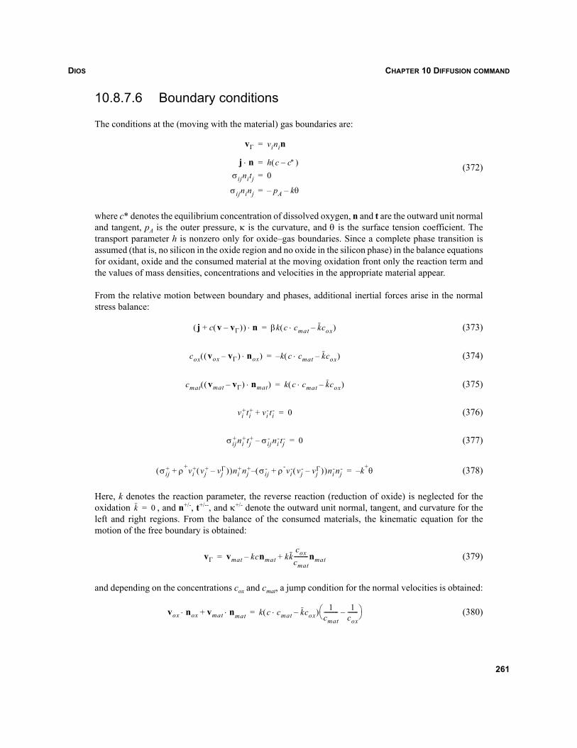
DIOS CHAPTER 10 DIFFUSION COMMAND
10.8.7.6 Boundary conditions
The conditions at the (moving with the material) gas boundaries are:
(372)
where c* denotes the equilibrium concentration of dissolved oxygen, n and t are the outward unit normaland tangent, pA is the outer pressure, κ is the curvature, and θ is the surface tension coefficient. Thetransport parameter h is nonzero only for oxide–gas boundaries. Since a complete phase transition isassumed (that is, no silicon in the oxide region and no oxide in the silicon phase) in the balance equationsfor oxidant, oxide and the consumed material at the moving oxidation front only the reaction term andthe values of mass densities, concentrations and velocities in the appropriate material appear.
From the relative motion between boundary and phases, additional inertial forces arise in the normalstress balance:
(373)
(374)
(375)
(376)
(377)
(378)
Here, k denotes the reaction parameter, the reverse reaction (reduction of oxide) is neglected for theoxidation , and n+/-, t+/--, and κ+/- denote the outward unit normal, tangent, and curvature for theleft and right regions. From the balance of the consumed materials, the kinematic equation for themotion of the free boundary is obtained:
(379)
and depending on the concentrations cox and cmat, a jump condition for the normal velocities is obtained:
(380)
vΓ vinin=
j n⋅ h c c*–( )=σijnitj 0=
σi jninj pA– kθ–=
j c v vΓ–( )+( ) n⋅ βk c cmat⋅ kcox–( )=
cox vox vΓ–( ) nox⋅( ) k c cmat⋅ kcox–( )–=
cmat vmat vΓ–( ) nmat⋅( ) k c c⋅ mat kcox–( )=
vi+ti
+ vi-ti
-+ 0=
σi j+ni
+tj+ σi j
- ni-tj
-– 0=
σij+ ρ+vi
+ vj+ vj
Γ–( )+( )ni+nj
+ σij- ρ-vi
- vj- vj
Γ–( )+( )ni-nj
-– k+θ–=
k 0=
vΓ vmat kcnmat kkcoxcmat----------nmat+–=
vox nox⋅ vmat n⋅ mat+ k c cmat⋅ kcox–( ) 1cmat---------- 1
cox-------–⎝ ⎠
⎛ ⎞=
261
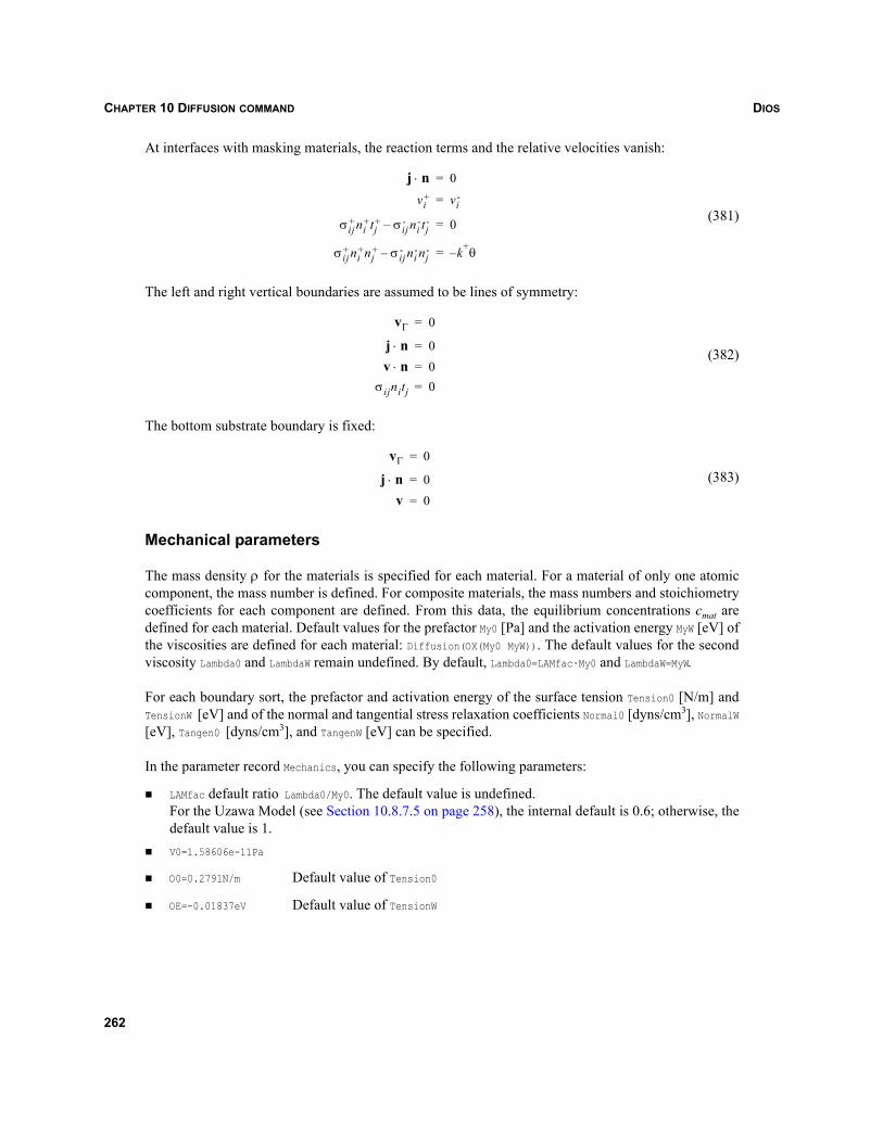
DIOSCHAPTER 10 DIFFUSION COMMAND
At interfaces with masking materials, the reaction terms and the relative velocities vanish:
(381)
The left and right vertical boundaries are assumed to be lines of symmetry:
(382)
The bottom substrate boundary is fixed:
(383)
Mechanical parameters
The mass density ρ for the materials is specified for each material. For a material of only one atomiccomponent, the mass number is defined. For composite materials, the mass numbers and stoichiometrycoefficients for each component are defined. From this data, the equilibrium concentrations cmat aredefined for each material. Default values for the prefactor My0 [Pa] and the activation energy MyW [eV] ofthe viscosities are defined for each material: Diffusion(OX(My0 MyW)). The default values for the secondviscosity Lambda0 and LambdaW remain undefined. By default, Lambda0=LAMfac·My0 and LambdaW=MyW.
For each boundary sort, the prefactor and activation energy of the surface tension Tension0 [N/m] andTensionW [eV] and of the normal and tangential stress relaxation coefficients Normal0 [dyns/cm3], NormalW[eV], Tangen0 [dyns/cm3], and TangenW [eV] can be specified.
In the parameter record Mechanics, you can specify the following parameters:
LAMfac default ratio Lambda0/My0. The default value is undefined. For the Uzawa Model (see Section 10.8.7.5 on page 258), the internal default is 0.6; otherwise, thedefault value is 1.V0=1.58606e-11Pa
O0=0.2791N/m Default value of Tension0
OE=-0.01837eV Default value of TensionW
j n⋅ 0=
vi+ vi
-=
σij+ni
+tj+ σij
- ni-tj
-– 0=
σi j+ ni
+nj+ σij
- ni-nj
-– k+– θ=
vΓ 0=
j n⋅ 0=v n⋅ 0=
σi jnitj 0=
vΓ 0=
j n⋅ 0=v 0=
262
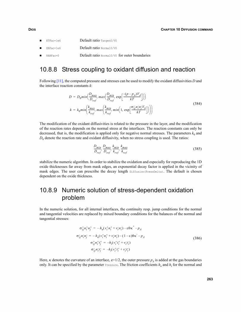
DIOS CHAPTER 10 DIFFUSION COMMAND
ETFac=1e6 Default ratio Tangen0/V0
ENFac=1e6 Default ratio Normal0/V0
RANFac=0 Default ratio Normal0/V0 for outer boundaries
10.8.8 Stress coupling to oxidant diffusion and reaction
Following [11], the computed pressure and stresses can be used to modify the oxidant diffusivities D andthe interface reaction constants k:
(384)
The modification of the oxidant diffusivities is related to the pressure in the layer, and the modificationof the reaction rates depends on the normal stress at the interfaces. The reaction constants can only bedecreased, that is, the modification is applied only for negative normal stresses. The parameters k0 andD0 denote the reaction rate and oxidant diffusivity, when no stress coupling is used. The ratios:
(385)
stabilize the numeric algorithm. In order to stabilize the oxidation and especially for reproducing the 1Doxide thicknesses far away from mask edges, an exponential decay factor is applied in the vicinity ofmask edges. The user can prescribe the decay length Diffusion(PressDelta). The default is chosendependent on the oxide thickness.
10.8.9 Numeric solution of stress-dependent oxidation problem
In the numeric solution, for all internal interfaces, the continuity resp. jump conditions for the normaland tangential velocities are replaced by mixed boundary conditions for the balances of the normal andtangential stresses:
(386)
Here, κ denotes the curvature of an interface, e=1/2, the outer pressure pA is added at the gas boundariesonly. It can be specified by the parameter Pressure. The friction coefficients hn and ht for the normal and
D D0minDmaxDref------------- max
DminDref------------
p pA–( )Vd–kT
-----------------------------exp,⎝ ⎠⎛ ⎞,⎝ ⎠
⎛ ⎞=
k k0minkmaxkref----------- max
kminkref---------- min 1
σij- ni
-nj-Vk
kT------------------------exp,⎝ ⎠
⎛ ⎞,⎝ ⎠⎜ ⎟⎛ ⎞
,⎝ ⎠⎜ ⎟⎛ ⎞
=
DminDref------------
DmaxDref-------------
kminkref----------
kmaxkref-----------, , ,
σij+ni
+nj+ hn vi
+ni+ vi
-ni-+( )– εθκ+ pA––=
σi j- ni
-nj- hn vi
+ni+ vi
-ni-+( )– 1 ε–( )θκ-– pA–=
σij+ni
+tj+ ht vi
+ti+ vi
-ti-+( )–=
σij- ni
-tj- ht vi
+ti+ vi
-ti-+( )–=
263
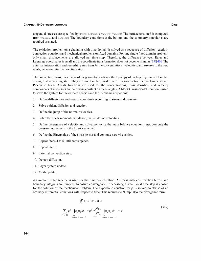
DIOSCHAPTER 10 DIFFUSION COMMAND
tangential stresses are specified by Normal0, NormalW, Tangen0, TangenW. The surface tension θ is computedfrom Tension0 and TensionW. The boundary conditions at the bottom and the symmetry boundaries arerequired as stated.
The oxidation problem on a changing with time domain is solved as a sequence of diffusion-reaction-convection equations and mechanical problems on fixed domains. For one single fixed domain problem,only small displacements are allowed per time step. Therefore, the difference between Euler andLagrange coordinates is small and the coordinate transformation does not become singular [39][40]. Theexternal interpolation and remeshing step transfer the concentrations, velocities, and stresses to the newmesh, generated for the next time step.
The convection terms, the change of the geometry, and even the topology of the layer system are handledduring that remeshing step. They are not handled inside the diffusion-reaction or mechanics solver.Piecewise linear Ansatz functions are used for the concentrations, mass densities, and velocitycomponents. The stresses are piecewise constant on the triangles. A block Gauss–Seidel iteration is usedto solve the system for the oxidant species and the mechanics equations:
1. Define diffusivities and reaction constants according to stress and pressure.
2. Solve oxidant diffusion and reaction.
3. Define the jump of the normal velocities.
4. Solve the linear momentum balance, that is, define velocities.
5. Define divergence of velocity and solve pointwise the mass balance equation, resp. compute thepressure increments in the Uzawa scheme.
6. Define the Eigenvalue of the stress tensor and compute new viscosities.
7. Repeat Steps 4 to 6 until convergence.
8. Repeat Step 1…
9. External convection step.
10. Dopant diffusion.
11. Layer system update.
12. Mesh update.
An implicit Euler scheme is used for the time discretization. All mass matrices, reaction terms, andboundary integrals are lumped. To ensure convergence, if necessary, a small local time step is chosenfor the solution of the mechanical problem. The hyperbolic equation for ρ is solved pointwise as anordinary differential equations with respect to time. This requires to ‘lump’ also the divergence term:
(387)td
dρ ρ vdiv+ 0= ⇒
ρ· β
Δ Ω∈∑ ϕaϕb xd
Δ∫ ρβ vi
γ
xi∂∂ϕγ ϕaϕb xd
Δ∫+ 0=
⎧ ⎪ ⎨ ⎪ ⎩ ⎧ ⎨ ⎩ ⎧ ⎪ ⎨ ⎪ ⎩
264
DIOS CHAPTER 10 DIFFUSION COMMAND
Improving the mechanics solver
The mechanics solver requires further improvement, testing, and stabilization: the linear and nonlinearsystems for the stress-dependent oxidation problem are difficult to solve. Sometimes, it shows unstablebehavior or requires small time steps and many iterations. Most of the known instabilities result fromthe coupling coefficients, especially for thin layers that are not well resolved by the mesh. So far, in allsimulations reducing or even completely switching off the stress coupling leads to stable modelbehavior. Completely switching off the nonlinear coupling leads to stable model behavior (but at thecosts of a linear model).
NOTE This is the default behavior in Dios. Users must define the Diffusion(Stressdependent=on)parameter to enable any stress-dependent oxidation simulation.
The default values for the activation volumes of the reaction rates, oxide diffusivities, and viscositiesare:
Diffusion(OX(O2(VD=38Angstr3),H2O(VD=38Angstr3),VMy=0)SIOX(O2(VK=8Angstr3),H2O(VK=8Angstr3))OXPO(O2(VK=8Angstr3),H2O(VK=8Angstr3))OXNI(O2(VK=8Angstr3),H2O(VK=8Angstr3))
)
The smaller these values are chosen, the less pronounced the instability (but also the nonlinear effect inthe oxidation). For large values, you may observe a positive feedback and a blowup of round-off errorsfrom the linear solver. For reasonable values, the instabilities often disappear during the simulation ifsome extra mesh points are used to discretize the layer, for example, for thicker oxides.
The impact of the coupling coefficients can be controlled also with the parameters:
Diffusion(Dmin/Dref=1e-3,Dmax/Dref=1,Kmin/Kref=1e-3,Kmax/Kref=1,MYmin/MYref=1e-3,MYmax/MYref=1
)
These restrict the deviation of the oxidant diffusivities and so on, from the parameter values, computedwithout stress coupling. Different sources contribute to the instability phenomenon:
To some extent, it is caused by the physical model(s), especially the nonlinear coupling terms. Thephysical model includes several nonlinear coupling terms between the computed stresses and thesolution of both the oxidant diffusion and reaction problem and the mechanics problem itself.
The material behavior (that is, the coefficients) is assumed to be nearly incompressible. This resultsin a small variation of the density. For the penalty method, it is obvious that mainly the solver erroris used in the pressure expression. In addition, for the mass balance model, the deviation from theconstant reference density is scaled with a large factor (OZP1) to obtain reasonable pressure values.Sometimes, the round-off error of the solver is left as a difference.
From a very small variation of the density, large variations of the oxidant diffusivities or reactionrates may result. This may indicate a nonphysical and unstable parameter fit to simulate oxide
265
DIOSCHAPTER 10 DIFFUSION COMMAND
contours close to the experimentally observed ones. Large values of the activation volumes VD andVK result in a positive feedback.
The chosen spatial discretization uses piecewise linear Ansatz functions for velocities on theelements and mass lumping for the time derivatives. The mass balance equation and the pressureupdates in the Uzawa algorithm are computed per node similar to an ODE by converting thedivergence given for the triangles into an average divergence for the mesh points. Both the chosenAnsatz functions and the lumping may be inappropriate for the problem.
A change of the refinement may change the result significantly. Usually, the refinement changes theprecise location of the pressure extrema but does not prevent the instability. This may indicate thatfor some eigenvalue close to zero, the corresponding eigenfunctions are insufficiently dampedduring the pressure-density iteration and the equations are simply not solved satisfactorily.
Not all derivatives are computed in the matrix. The derivatives of the implicit material law for thestress tensor or (dependency of the viscosity on the stress) are not resolved properly.
Some badly shaped triangles in the vicinity of interfaces may cause problems for the iterationprocess for the dopant diffusion. Then, the time step collapses until the problematic mesh elementdisappears after a series of time steps (the moving interfaces cut the triangles in a different way) andthe time step recovers.
10.9 Glass reflowIn the boundary conditions for the mechanical problem in oxidation simulation, a surface tension termis used. By default, an inert diffusion Atmosphere=N2 is simulated without modification of the layerstructure. No mechanical problem is solved in this case. This can be changed. For example:
Diffusion(Mechanics(AlwaysMechanics=on))
can be specified to simulate the reflow of highly doped oxide layers during an inert anneal step. Themechanical problem is solved, but in this situation, the old stresses from preceding steps and the surfacetension are the only driving forces for the deformation. No jumps occur at the interfaces. A concentrationdependency of the mechanical parameters has not yet been included in Dios. To obtain the desired refloweffect, you may be forced to increase the default values of the surface tension O0 and to decrease thedefault value of the oxide viscosity.
Alternatively, a simple parameter model can be used to simulate the glass reflow:
Diffusion(Reflow=4, MaxDist=0.95)
The parameter MaxDist defines a reduction factor for the angles between neighboring intervals on theoxide–gas boundaries in each time step. Values close to 1 ensure small deformations of the layerstructure. The parameter models Reflow=1,2,3 use a ‘surface diffusion’ or ‘diffusion of the curvature’ assuggested [34]. They proved to be unstable and very sensitive to the discretization. These parametermodels have no physical background, simply the oxide–gas contours are smoothened.
266
DIOS CHAPTER 10 DIFFUSION COMMAND
NOTE The consistency checks in these parameter models, for example, for very thin oxide layersaround sharp corners, may still be insufficient. The triple points oxide-material-gas remainimmobile.
10.10 SilicidationIf a metal layer and silicon are in contact during an anneal step, the growth of a silicide layer is simulated.Both the parameter model, and the diffusion-reaction and mechanics models have been generalized tohandle silicidation processes.
In the parameter model, silicidation processes are not modeled, only a very simple modification of thelayer system is performed. The expected final thickness of the silicide layer is computed, using amodified Deal–Grove law [12]. No analysis of mask edges is performed as in the oxidation, but insteadall metal-silicon or metal-polysilicon boundaries are treated in a single step. The string algorithm is usedto ‘etch’ the entire silicide thickness into the silicon or polysilicon layers. The metal layer remainsunchanged. This ‘etching’ step is performed before the first time step of the diffusion and the entirediffusion process is computed with a fixed layer structure and with inert ambient. If a silicide layer ispresent during an oxidation, the usual parameter model is applied. A silicon layer underneath the silicideis consumed; the silicide layer moves and changes its thickness by a small amount. The oxide layer isgrown on top of the silicide.
The 2D diffusion/reaction model and the mechanics solvers can be used also to simulate the silicidationprocess. In Dios, one of the metals tantalum, cobalt, tungsten, titanium, platinum, or molybdenum canbe deposited in a layer structure. Depending on the metal, the dissolution, transport, and reaction ofmetal or silicon atoms in the growing silicide and at its boundaries is simulated. This model is selectedby using:
Diffusion(Models(Silicidation(ModDiffSili=Diffusion)))
For each metal, a specific set of internal default values is used. The default values are selected when themetal is specified in a Deposit command. The default diffusing species and internal model parametersare stored in the ME(...) and MEMS(...) data records. Only one of the metals, forming silicides, and thecorresponding silicide can be present in a structure at a time.
Default values for molybdenum silicide have been adapted in [12]. They depend on implantation stepsafter the metal deposition. Default model parameters for the other metals have been taken from theliterature [53].
The silicidation model used in Dios does not include:
Bulk reactions, changing the stoichiometry of already grown silicide
Formation of different (silicon-rich or metal-rich) modifications of silicide
Interaction with silicon point defects
267
DIOSCHAPTER 10 DIFFUSION COMMAND
Initial silicide layers are generated at each interface between metal and silicon, polysilicon or SG. Theinitial silicide thickness is given by an Arrhenius law. The prefactor and the activation energy Thick0 andThickW can be specified for each of the boundary sorts SIMS, POMS, SGMS. By default, 2 nm are generated.
Since there is never any oxidant species and a diffusing species for silicidation defined in the samematerial, the dissolved metal atoms in silicide regions are stored on the OTotal dataset and the dissolvedsilicon atoms are stored on the H2OTotal dataset. Dopant diffusion in silicide is modeled in analogy todopant diffusion in polysilicon (see Section 10.3.7 on page 217).
10.10.1 Silicon as diffusing species
Silicon atoms can dissolve at an interface between silicide and silicon, polysilicon, or a silicon-germanium layer into the growing silicide layer. They diffuse through the silicide and react with theimmobile metal at the metal-silicide interfaces.
Due to the imbalances of the material conversion rates, the mechanical deformation of the structure mustbe simulated:
(388)
As for oxidation, the reverse reaction at the silicide-metal interfaces is neglected: . Thestoichiometry coefficient β can be specified as:
Diffusion(MS(Stoichiometry(S1 S2)))
The first value is used for the metal, the second, for the silicon. The reaction rate kmat of the dissolutionof silicon at the interfaces can be specified as STC0 and STCW. The parameter C* prescribes the value of
at these interfaces, and VK prescribes the activation volume for the stress coupling:
DIFFusion(SIMS(Silicon(STC0 STCW C* VK)))DIFFusion(POMS(Silicon(STC0 STCW C* VK)))DIFFusion(SGMS(Silicon(STC0 STCW C* VK)))
The reaction rate at the metal–silicide interface and the activation volume for the stress dependencyof the reaction rate can be specified with the parameters STC0 and STCW for the boundary sort MEMS:
DIFFusion(MEMS(Silicon(STC0 STCW VK))
The imbalances of the consumption and production rates of the involved layer materials at the material-silicide and silicide-metal interfaces lead to a mechanical deformation of the layer structure at thematerial-silicide interface:
(389)
t∂∂c j cv+( )div+ 0=
j c vms vΓ–( )+( ) nms⋅ kmat c kmatcmat–( ) 0 at the silicon-silicide interface<=
j c vms vΓ–( )+( ) nms⋅ βkme c c⋅ me kmecms–( ) 0 at the silicide-metal interface>=
kme 0=
kmat cmat⋅
kme
cmat vmat vΓ–( ) n⋅ mat( ) kmat– c kmatcmat–( ) 0<=
cms vms vΓ–( ) nms⋅( ) 0=
268
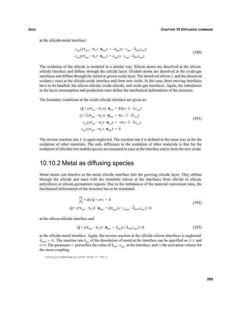
DIOS CHAPTER 10 DIFFUSION COMMAND
at the silicide-metal interface:
(390)
The oxidation of the silicide is modeled in a similar way. Silicon atoms are dissolved at the silicon-silicide interface and diffuse through the silicide layer. Oxidant atoms are dissolved at the oxide-gasinterfaces and diffuse through the initial or grown oxide layer. The dissolved silicon and the dissolvedoxidant c react at the silicide-oxide interface and form new oxide. In this case, three moving interfaceshave to be handled: the silicon-silicide, oxide-silicide, and oxide-gas interfaces. Again, the imbalancesin the layer consumption and production rates define the mechanical deformation of the structure.
The boundary conditions at the oxide-silicide interface are given as:
(391)
The inverse reaction rate is again neglected. The reaction rate k is defined in the same way as for theoxidation of other materials. The only difference to the oxidation of other materials is that for theoxidation of silicides two mobile species are assumed to react at the interface and to form the new oxide.
10.10.2 Metal as diffusing species
Metal atoms can dissolve at the metal silicide interface into the growing silicide layer. They diffusethrough the silicide and react with the immobile silicon at the interfaces from silicide to silicon,polysilicon or silicon-germanium regions. Due to the imbalances of the material conversion rates, themechanical deformation of the structure has to be simulated:
(392)
at the silicon-silicide interface and:
(393)
at the silicide-metal interface. Again, the reverse reaction at the silicide-silicon interfaces is neglected:. The reaction rate kme of the dissolution of metal at the interface can be specified as STC0 and
STCW. The parameter C* prescribes the value of at the interface, and VK the activation volume forthe stress coupling:
Diffusion(MEMS(Metal(STC0 STCW C* VK)))
cms vms vΓ–( ) nms⋅( ) kme– c c⋅ me kmecms–( )=
cme vme vΓ–( ) nme⋅( ) kme c cme⋅ kmecms–( )=
c
j c vox vΓ–( )+( ) nox⋅ βk c c⋅ kcox–( )=
j c vms vΓ–( )+( ) nms⋅ k c c⋅ kcox–( )=
cox vox vΓ–( ) nox⋅( ) k– c c⋅ kcox–( )=
cms vms vΓ–( ) nms⋅( ) 0=
k
t∂∂c j cv+( )div+ 0=
j c vms vΓ–( )+( ) nms⋅ βkmat c cmat⋅ kmatcms–( ) 0>=
j c vms vΓ–( )+( ) nms⋅ kme c kmecme–( ) 0<=
kmat 0=kme cme⋅
269
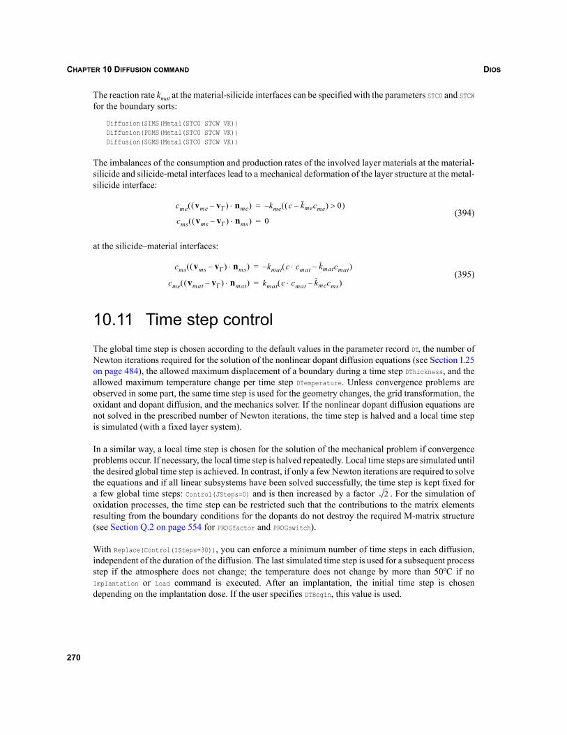
DIOSCHAPTER 10 DIFFUSION COMMAND
The reaction rate kmat at the material-silicide interfaces can be specified with the parameters STC0 and STCWfor the boundary sorts:
Diffusion(SIMS(Metal(STC0 STCW VK))Diffusion(POMS(Metal(STC0 STCW VK))Diffusion(SGMS(Metal(STC0 STCW VK))
The imbalances of the consumption and production rates of the involved layer materials at the material-silicide and silicide-metal interfaces lead to a mechanical deformation of the layer structure at the metal-silicide interface:
(394)
at the silicide–material interfaces:
(395)
10.11 Time step controlThe global time step is chosen according to the default values in the parameter record DT, the number ofNewton iterations required for the solution of the nonlinear dopant diffusion equations (see Section I.25on page 484), the allowed maximum displacement of a boundary during a time step DThickness, and theallowed maximum temperature change per time step DTemperature. Unless convergence problems areobserved in some part, the same time step is used for the geometry changes, the grid transformation, theoxidant and dopant diffusion, and the mechanics solver. If the nonlinear dopant diffusion equations arenot solved in the prescribed number of Newton iterations, the time step is halved and a local time stepis simulated (with a fixed layer system).
In a similar way, a local time step is chosen for the solution of the mechanical problem if convergenceproblems occur. If necessary, the local time step is halved repeatedly. Local time steps are simulated untilthe desired global time step is achieved. In contrast, if only a few Newton iterations are required to solvethe equations and if all linear subsystems have been solved successfully, the time step is kept fixed fora few global time steps: Control(JSteps=0) and is then increased by a factor . For the simulation ofoxidation processes, the time step can be restricted such that the contributions to the matrix elementsresulting from the boundary conditions for the dopants do not destroy the required M-matrix structure(see Section Q.2 on page 554 for PROGfactor and PROGswitch).
With Replace(Control(ISteps=30)), you can enforce a minimum number of time steps in each diffusion,independent of the duration of the diffusion. The last simulated time step is used for a subsequent processstep if the atmosphere does not change; the temperature does not change by more than 50oC if noImplantation or Load command is executed. After an implantation, the initial time step is chosendepending on the implantation dose. If the user specifies DTBegin, this value is used.
cme vme vΓ–( ) nme⋅( ) kme– c kmecme–( ) 0>( )=
cms vms vΓ–( ) nms⋅( ) 0=
cms vms vΓ–( ) nms⋅( ) kmat– c c⋅ mat kmatcmat–( )=
cme vmat vΓ–( ) nmat⋅( ) kmat c cmat⋅ kmecms–( )=
2
270
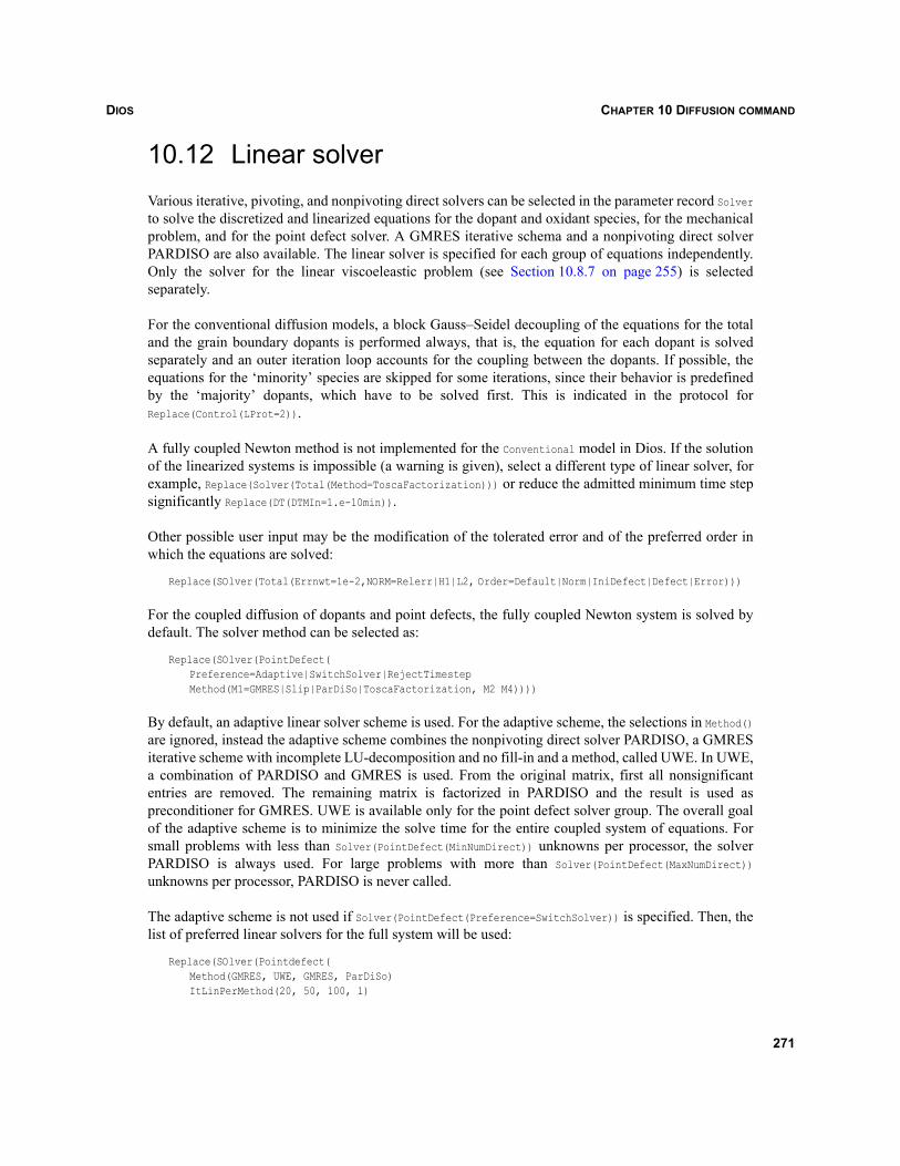
DIOS CHAPTER 10 DIFFUSION COMMAND
10.12 Linear solverVarious iterative, pivoting, and nonpivoting direct solvers can be selected in the parameter record Solverto solve the discretized and linearized equations for the dopant and oxidant species, for the mechanicalproblem, and for the point defect solver. A GMRES iterative schema and a nonpivoting direct solverPARDISO are also available. The linear solver is specified for each group of equations independently.Only the solver for the linear viscoeleastic problem (see Section 10.8.7 on page 255) is selectedseparately.
For the conventional diffusion models, a block Gauss–Seidel decoupling of the equations for the totaland the grain boundary dopants is performed always, that is, the equation for each dopant is solvedseparately and an outer iteration loop accounts for the coupling between the dopants. If possible, theequations for the ‘minority’ species are skipped for some iterations, since their behavior is predefinedby the ‘majority’ dopants, which have to be solved first. This is indicated in the protocol forReplace(Control(LProt=2)).
A fully coupled Newton method is not implemented for the Conventional model in Dios. If the solutionof the linearized systems is impossible (a warning is given), select a different type of linear solver, forexample, Replace(Solver(Total(Method=ToscaFactorization))) or reduce the admitted minimum time stepsignificantly Replace(DT(DTMIn=1.e-10min)).
Other possible user input may be the modification of the tolerated error and of the preferred order inwhich the equations are solved:
Replace(SOlver(Total(Errnwt=1e-2,NORM=Relerr|H1|L2, Order=Default|Norm|IniDefect|Defect|Error)))
For the coupled diffusion of dopants and point defects, the fully coupled Newton system is solved bydefault. The solver method can be selected as:
Replace(SOlver(PointDefect(Preference=Adaptive|SwitchSolver|RejectTimestepMethod(M1=GMRES|Slip|ParDiSo|ToscaFactorization, M2 M4))))
By default, an adaptive linear solver scheme is used. For the adaptive scheme, the selections in Method()are ignored, instead the adaptive scheme combines the nonpivoting direct solver PARDISO, a GMRESiterative scheme with incomplete LU-decomposition and no fill-in and a method, called UWE. In UWE,a combination of PARDISO and GMRES is used. From the original matrix, first all nonsignificantentries are removed. The remaining matrix is factorized in PARDISO and the result is used aspreconditioner for GMRES. UWE is available only for the point defect solver group. The overall goalof the adaptive scheme is to minimize the solve time for the entire coupled system of equations. Forsmall problems with less than Solver(PointDefect(MinNumDirect)) unknowns per processor, the solverPARDISO is always used. For large problems with more than Solver(PointDefect(MaxNumDirect))unknowns per processor, PARDISO is never called.
The adaptive scheme is not used if Solver(PointDefect(Preference=SwitchSolver)) is specified. Then, thelist of preferred linear solvers for the full system will be used:
Replace(SOlver(Pointdefect(Method(GMRES, UWE, GMRES, ParDiSo)ItLinPerMethod(20, 50, 100, 1)
271
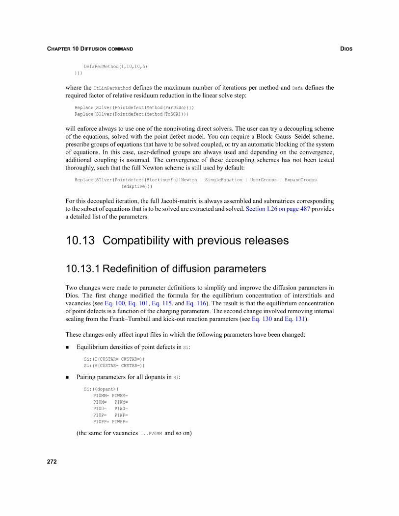
DIOSCHAPTER 10 DIFFUSION COMMAND
DefaPerMethod(1,10,10,5))))
where the ItLinPerMethod defines the maximum number of iterations per method and Defa defines therequired factor of relative residuum reduction in the linear solve step:
Replace(SOlver(Pointdefect(Method(ParDiSo))))Replace(SOlver(Pointdefect(Method(ToSCA))))
will enforce always to use one of the nonpivoting direct solvers. The user can try a decoupling schemeof the equations, solved with the point defect model. You can require a Block–Gauss–Seidel scheme,prescribe groups of equations that have to be solved coupled, or try an automatic blocking of the systemof equations. In this case, user-defined groups are always used and depending on the convergence,additional coupling is assumed. The convergence of these decoupling schemes has not been testedthoroughly, such that the full Newton scheme is still used by default:
Replace(SOlver(Pointdefect(Blocking=FullNewton | SingleEquation | UserGroups | ExpandGroups|Adaptive)))
For this decoupled iteration, the full Jacobi-matrix is always assembled and submatrices correspondingto the subset of equations that is to be solved are extracted and solved. Section I.26 on page 487 providesa detailed list of the parameters.
10.13 Compatibility with previous releases
10.13.1 Redefinition of diffusion parameters
Two changes were made to parameter definitions to simplify and improve the diffusion parameters inDios. The first change modified the formula for the equilibrium concentration of interstitials andvacancies (see Eq. 100, Eq. 101, Eq. 115, and Eq. 116). The result is that the equilibrium concentrationof point defects is a function of the charging parameters. The second change involved removing internalscaling from the Frank–Turnbull and kick-out reaction parameters (see Eq. 130 and Eq. 131).
These changes only affect input files in which the following parameters have been changed:
Equilibrium densities of point defects in Si:
Si:(I(C0STAR= CWSTAR=))Si:(V(C0STAR= CWSTAR=))
Pairing parameters for all dopants in Si:
Si:(<dopant>(PI0MM= PIWMM=PI0M= PIWM=PI00= PIW0=PI0P= PIWP=PI0PP= PIWPP=
(the same for vacancies ...PV0MM and so on)
272
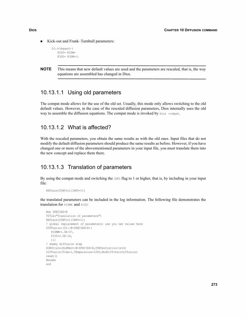
DIOS CHAPTER 10 DIFFUSION COMMAND
Kick-out and Frank–Turnbull parameters:
Si:(<dopant>(K2S0= K2SW=K3S0= K3SW=))
NOTE This means that new default values are used and the parameters are rescaled, that is, the wayequations are assembled has changed in Dios.
10.13.1.1 Using old parameters
The compat mode allows for the use of the old set. Usually, this mode only allows switching to the olddefault values. However, in the case of the rescaled diffusion parameters, Dios internally uses the oldway to assemble the diffusion equations. The compat mode is invoked by dios -compat.
10.13.1.2 What is affected?
With the rescaled parameters, you obtain the same results as with the old ones. Input files that do notmodify the default diffusion parameters should produce the same results as before. However, if you havechanged one or more of the abovementioned parameters in your input file, you must translate them intothe new concept and replace them there.
10.13.1.3 Translation of parameters
By using the compat mode and switching the INFO flag to 1 or higher, that is, by including in your inputfile:
REPLace(CONTrol(INFO=1))
the translated parameters can be included in the log information. The following file demonstrates thetranslation for PI0MM and PI00:
#do SPECIES=BTITle("Translation of parameters")REPLace(CONTrol(INFO=1))! global replacement of parameters: use you own values hereDIFFusion:(SI:(@<SPECIES>@:( PI0MM=1.0E-07, PI00=2.0E-14, )))! dummy diffusion stepSUBStrate(ELEMent=@<SPECIES>@,CONCentration=1e14)DIFFusion(Time=1,TEmperature=1000,ModDiff=PairDiffusion)reset()#enddoend
273
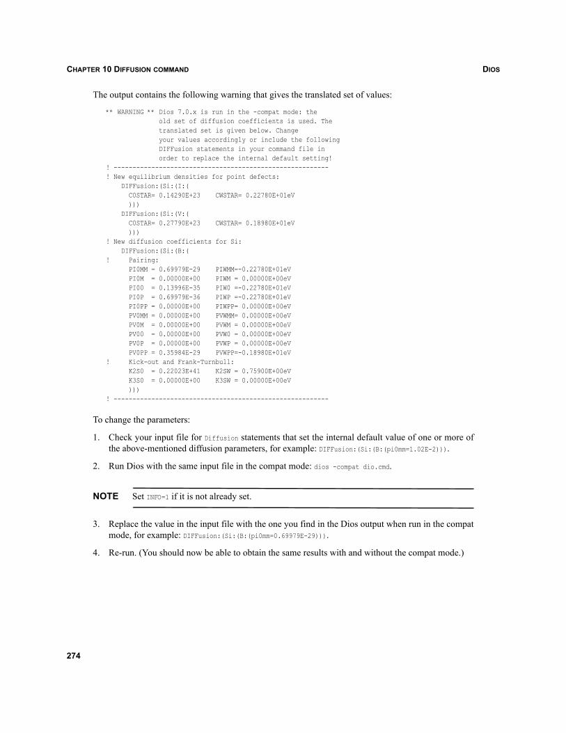
DIOSCHAPTER 10 DIFFUSION COMMAND
The output contains the following warning that gives the translated set of values:
** WARNING ** Dios 7.0.x is run in the -compat mode: the old set of diffusion coefficients is used. The translated set is given below. Change your values accordingly or include the following DIFFusion statements in your command file in order to replace the internal default setting!! ---------------------------------------------------------! New equilibrium densities for point defects: DIFFusion:(Si:(I:( C0STAR= 0.14290E+23 CWSTAR= 0.22780E+01eV ))) DIFFusion:(Si:(V:( C0STAR= 0.27790E+23 CWSTAR= 0.18980E+01eV )))! New diffusion coefficients for Si: DIFFusion:(Si:(B:(! Pairing: PI0MM = 0.69979E-29 PIWMM=-0.22780E+01eV PI0M = 0.00000E+00 PIWM = 0.00000E+00eV PI00 = 0.13996E-35 PIW0 =-0.22780E+01eV PI0P = 0.69979E-36 PIWP =-0.22780E+01eV PI0PP = 0.00000E+00 PIWPP= 0.00000E+00eV PV0MM = 0.00000E+00 PVWMM= 0.00000E+00eV PV0M = 0.00000E+00 PVWM = 0.00000E+00eV PV00 = 0.00000E+00 PVW0 = 0.00000E+00eV PV0P = 0.00000E+00 PVWP = 0.00000E+00eV PV0PP = 0.35984E-29 PVWPP=-0.18980E+01eV! Kick-out and Frank-Turnbull: K2S0 = 0.22023E+41 K2SW = 0.75900E+00eV K3S0 = 0.00000E+00 K3SW = 0.00000E+00eV )))! ---------------------------------------------------------
To change the parameters:
1. Check your input file for Diffusion statements that set the internal default value of one or more ofthe above-mentioned diffusion parameters, for example: DIFFusion:(Si:(B:(pi0mm=1.02E-2))).
2. Run Dios with the same input file in the compat mode: dios -compat dio.cmd.
NOTE Set INFO=1 if it is not already set.
3. Replace the value in the input file with the one you find in the Dios output when run in the compatmode, for example: DIFFusion:(Si:(B:(pi0mm=0.69979E-29))).
4. Re-run. (You should now be able to obtain the same results with and without the compat mode.)
274
DIOS CHAPTER 11 LOAD COMMAND
Dios
CHAPTER 11 Load command
11.1 OverviewThe Load command is used to load:
Dios dmp files from previous simulations.
Analytic profiles, profiles from external meshes (submeshes).
DF–ISE grid and data files (grd, dat).
3D Mesh command files (cmd).
3D DF–ISE or OMEGA boundary files (bnd, bound).
A file name must always be specified. The parameter Type or the recommended file extension (seeSection 2.4 on page 54) can be used to select the proper load function. Loading a Dios dmp file is thedefault. Appendix J on page 501 lists the Load command parameters.
11.2 Loading a dmp fileWhen loading a Dios dmp file, grid, layer structure, doping profiles and the set of default parameters thatwere used in the simulation are read from the file, and the simulation can continue. The save files canbe compressed or gzip’ed. Incompatibilities of the storage requirements between loaded file and currentDios run are indicated and corrected internally. Incompatibilities of old save files with newer programversions frequently indicate modifications in the parameter list of commands. Then, the default valuesof the parameters cannot be read from the dmp file, and the changes of default values that had been madefor the simulation have to be repeated after loading the file. Other incompatibilities in the dmp files arehandled by different internal version numbers in the file. Appropriate warning messages are displayed.
Dios tries to open a file in two different byte orders in order to load a binary file from, for example, aLinux or PC version on a UNIX machine. If loading the file as binary file does not work, Dios tries toopen and read the file as an ASCII file. The dmp file contains also the command and mask files that wereused to generate the file (it does not include 1D profiles used in a Load or an Implantation command).These files can be extracted from the dmp file with the command:
Load(File=Filename, Extract=on)
275
DIOSCHAPTER 11 LOAD COMMAND
11.3 Loading DF–ISE and other external filesSimulation results saved in DF–ISE format (or in any other supported external file format) can be loadedinto Dios. The file names can be specified on the command line:
dios file.grd file.datdios aaa.tifdios aaa.exp
The files can also be loaded from the Load command:
Load(File=file.grd DataFile=file.dat Type=DFISE)Load(file=aaa.tif,type=tif)Load(file=aaa.exp,type=exp)
A DF–ISE grid can be 2D or 3D. All other formats are 2D. By default, the same file basename isassumed, only the extension is changed.
The user can specify as File the name of the grd file and as DataFile the name of the dat file.Load(File=xxx,Type=grd) can be used only to load a grd file. After this is performed,Load(File=xxx,Type=dat) can be used to load a corresponding dat file.
Upon loading a 2D external file (DF–ISE, tif, exp,...) from the command line, the loaded grid isconverted into a Dios UTRI grid. Loading DF–ISE files into Dios may change the numbering of thevertices since Dios always generates multiple points at material interfaces and the outer boundary. It mayalso change the numbering of the elements if a mixed element grid is loaded, since all rectangles are splitinto two triangles. Upon loading a file, Dios should not change any data values or coordinates. From thegrid, the outer boundary, the material interfaces, and the topology of the structure are extracted andconverted into a Dios layer structure. This can be used to load externally defined structures ornonisotropically refined meshes.
If an external file is loaded from the load command, specify the parameter Load(SubMesh=no,...) to ensurethat the grid is converted and the layer structure is extracted. By default, Load(SubMesh=undefined,...).Only Dios dmp files are, by default, loaded as new grid and layer structure. All other external files areloaded by default as submesh and used only to interpolate data from (see Section 11.5 on page 277).
11.4 Loading 3D simulationsThe Load command can be used to switch from 2D to 3D, or to change the structure used in the 3Dsimulation. Since for 3D gridding, the library version or the stand-alone version of Mesh is used, the usercan provide the name of a command file, containing refinement information: Load(File=..., Type=cmd).
A DF–ISE bnd file or the old style 3D OMEGA bound file can be loaded. In both cases, the 3D gridgenerator Mesh is called to generate a volume mesh for the structure. If the user has already loaded acommand file, it is copied and extended by Dios to contain also the doping information, either thesweeping from a (single) 2D submesh or the interpolation of the current 3D submesh. If no commandfile had been loaded, Dios generates a command file, which contains a subset of the currently used 2Drefinement parameters, translated (as much as possible) into Mesh syntax. After generating the 3D grid
276
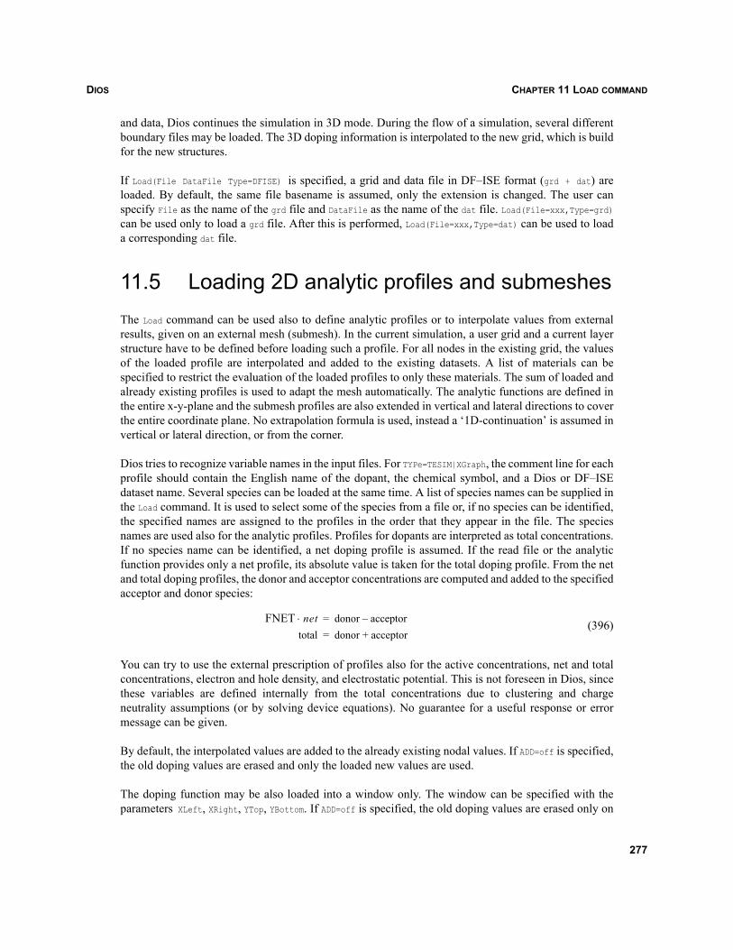
DIOS CHAPTER 11 LOAD COMMAND
and data, Dios continues the simulation in 3D mode. During the flow of a simulation, several differentboundary files may be loaded. The 3D doping information is interpolated to the new grid, which is buildfor the new structures.
If Load(File DataFile Type=DFISE) is specified, a grid and data file in DF–ISE format (grd + dat) areloaded. By default, the same file basename is assumed, only the extension is changed. The user canspecify File as the name of the grd file and DataFile as the name of the dat file. Load(File=xxx,Type=grd)can be used only to load a grd file. After this is performed, Load(File=xxx,Type=dat) can be used to loada corresponding dat file.
11.5 Loading 2D analytic profiles and submeshesThe Load command can be used also to define analytic profiles or to interpolate values from externalresults, given on an external mesh (submesh). In the current simulation, a user grid and a current layerstructure have to be defined before loading such a profile. For all nodes in the existing grid, the valuesof the loaded profile are interpolated and added to the existing datasets. A list of materials can bespecified to restrict the evaluation of the loaded profiles to only these materials. The sum of loaded andalready existing profiles is used to adapt the mesh automatically. The analytic functions are defined inthe entire x-y-plane and the submesh profiles are also extended in vertical and lateral directions to coverthe entire coordinate plane. No extrapolation formula is used, instead a ‘1D-continuation’ is assumed invertical or lateral direction, or from the corner.
Dios tries to recognize variable names in the input files. For TYPe=TESIM|XGraph, the comment line for eachprofile should contain the English name of the dopant, the chemical symbol, and a Dios or DF–ISEdataset name. Several species can be loaded at the same time. A list of species names can be supplied inthe Load command. It is used to select some of the species from a file or, if no species can be identified,the specified names are assigned to the profiles in the order that they appear in the file. The speciesnames are used also for the analytic profiles. Profiles for dopants are interpreted as total concentrations.If no species name can be identified, a net doping profile is assumed. If the read file or the analyticfunction provides only a net profile, its absolute value is taken for the total doping profile. From the netand total doping profiles, the donor and acceptor concentrations are computed and added to the specifiedacceptor and donor species:
(396)
You can try to use the external prescription of profiles also for the active concentrations, net and totalconcentrations, electron and hole density, and electrostatic potential. This is not foreseen in Dios, sincethese variables are defined internally from the total concentrations due to clustering and chargeneutrality assumptions (or by solving device equations). No guarantee for a useful response or errormessage can be given.
By default, the interpolated values are added to the already existing nodal values. If ADD=off is specified,the old doping values are erased and only the loaded new values are used.
The doping function may be also loaded into a window only. The window can be specified with theparameters XLeft, XRight, YTop, YBottom. If ADD=off is specified, the old doping values are erased only on
FNET net⋅ donor acceptor–=total donor acceptor+=
277
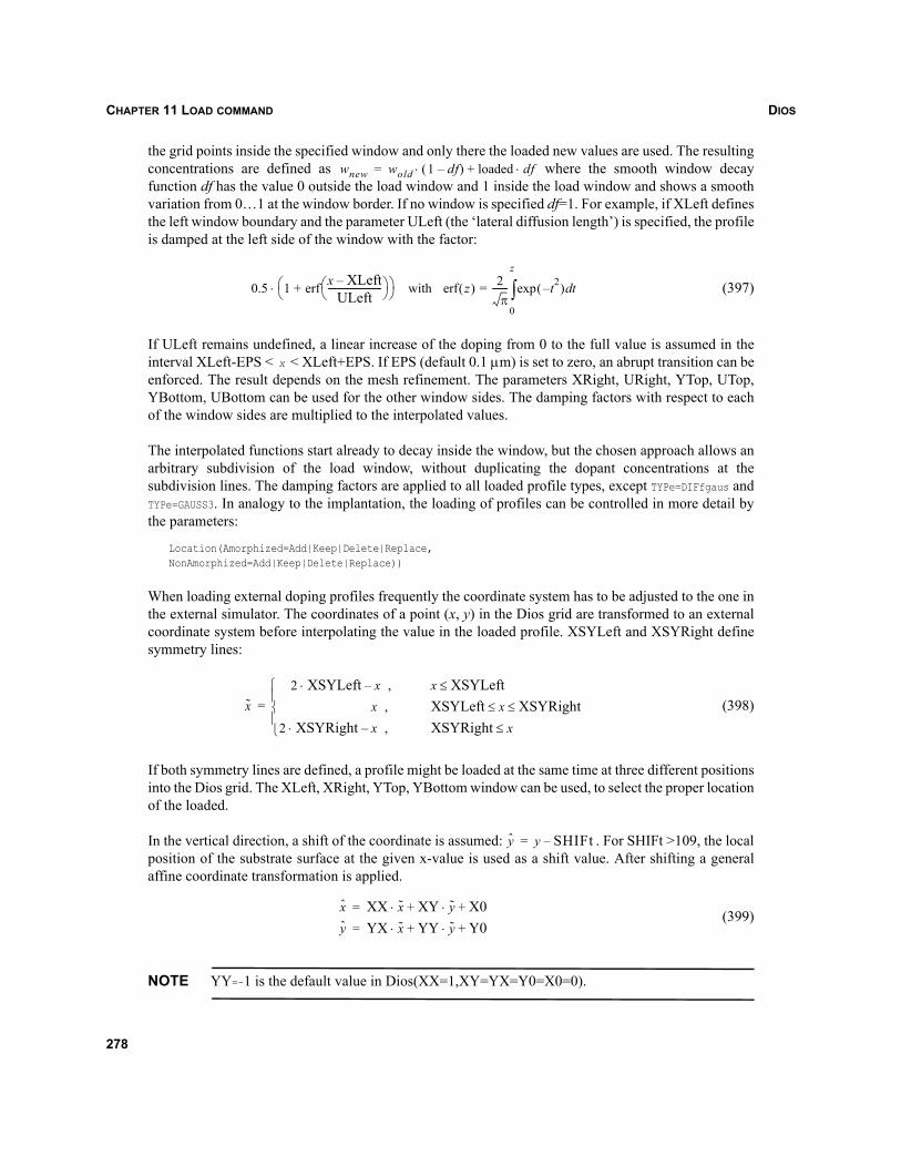
DIOSCHAPTER 11 LOAD COMMAND
the grid points inside the specified window and only there the loaded new values are used. The resultingconcentrations are defined as where the smooth window decayfunction df has the value 0 outside the load window and 1 inside the load window and shows a smoothvariation from 0…1 at the window border. If no window is specified df=1. For example, if XLeft definesthe left window boundary and the parameter ULeft (the ‘lateral diffusion length’) is specified, the profileis damped at the left side of the window with the factor:
(397)
If ULeft remains undefined, a linear increase of the doping from 0 to the full value is assumed in theinterval XLeft-EPS < x < XLeft+EPS. If EPS (default 0.1 μm) is set to zero, an abrupt transition can beenforced. The result depends on the mesh refinement. The parameters XRight, URight, YTop, UTop,YBottom, UBottom can be used for the other window sides. The damping factors with respect to eachof the window sides are multiplied to the interpolated values.
The interpolated functions start already to decay inside the window, but the chosen approach allows anarbitrary subdivision of the load window, without duplicating the dopant concentrations at thesubdivision lines. The damping factors are applied to all loaded profile types, except TYPe=DIFfgaus andTYPe=GAUSS3. In analogy to the implantation, the loading of profiles can be controlled in more detail bythe parameters:
Location(Amorphized=Add|Keep|Delete|Replace,NonAmorphized=Add|Keep|Delete|Replace))
When loading external doping profiles frequently the coordinate system has to be adjusted to the one inthe external simulator. The coordinates of a point (x, y) in the Dios grid are transformed to an externalcoordinate system before interpolating the value in the loaded profile. XSYLeft and XSYRight definesymmetry lines:
(398)
If both symmetry lines are defined, a profile might be loaded at the same time at three different positionsinto the Dios grid. The XLeft, XRight, YTop, YBottom window can be used, to select the proper locationof the loaded.
In the vertical direction, a shift of the coordinate is assumed: . For SHIFt >109, the localposition of the substrate surface at the given x-value is used as a shift value. After shifting a generalaffine coordinate transformation is applied.
(399)
NOTE YY=–1 is the default value in Dios(XX=1,XY=YX=Y0=X0=0).
wnew wold 1 df–( )⋅ loaded df⋅+=
0.5 1 x XLeft–ULeft
------------------------⎝ ⎠⎛ ⎞erf+⎝ ⎠
⎛ ⎞ with z( )erf 2π
------- t2–( )exp td0
z
∫=⋅
x2 XSYLeft x , –⋅ x XSYLeft≤
x , XSYLeft x XSYRight≤ ≤
2 XSYRight x , –⋅ XSYRight x≤⎩⎪⎨⎪⎧
=
y y SHIFt–=
x XX x⋅ XY y⋅ X0+ +=y YX x⋅ YY y⋅ Y0+ +=
278
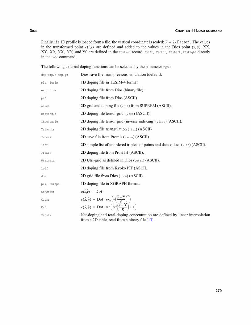
DIOS CHAPTER 11 LOAD COMMAND
Finally, if a 1D profile is loaded from a file, the vertical coordinate is scaled: . The valuesin the transformed point are defined and added to the values in the Dios point (x, y). XX,XY, X0, YX, YY, and Y0 are defined in the Control record, Shift, Factor, XSyLeft, XSyRight directlyin the Load command.
The following external doping functions can be selected by the parameter Type:
dmp dmp.Z dmp.gz Dios save file from previous simulation (default).
plt, Tesim 1D doping file in TESIM-4 format.
exp, dios 2D doping file from Dios (binary file).
prf 2D doping file from Dios (ASCII).
Alien 2D grid and doping file (.tif) from SUPREM (ASCII).
Rectangle 2D doping file tensor grid. (.rec) (ASCII).
IRectangle 2D doping file tensor grid (inverse indexing) (.irec) (ASCII).
Triangle 2D doping file triangulation (.tri) (ASCII).
Promis 2D save file from Promis (.save) (ASCII).
List 2D simple list of unordered triplets of points and data values (.lis) (ASCII).
ProETH 2D doping file from ProETH (ASCII).
Utrigrid 2D Utri-grid as defined in Dios (.utri) (ASCII).
kpif 2D doping file from Kyoko PIF (ASCII).
dom 2D grid file from Dios (.dom) (ASCII).
plx, XGraph 1D doping file in XGRAPH format.
Constant
Gauss
Erf
Prosim Net-doping and total-doping concentration are defined by linear interpolationfrom a 2D table, read from a binary file [13].
y y Factor⋅=c x y( , )
c x y( , ) Dot=
c x y,( ) Dot y Y–S
-------------⎝ ⎠⎛ ⎞ 2
–⎝ ⎠⎛ ⎞exp⋅=
c x y,( ) Dot 0.5 y Y–S
-------------⎝ ⎠⎛ ⎞ 1+erf⎝ ⎠
⎛ ⎞⋅=
279
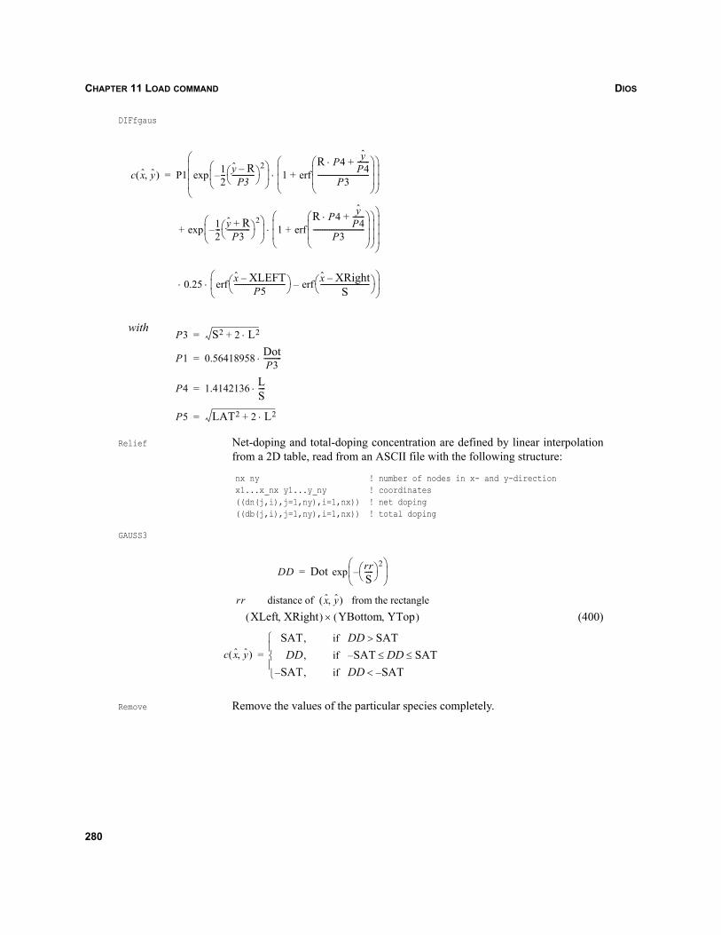
DIOSCHAPTER 11 LOAD COMMAND
DIFfgaus
Relief Net-doping and total-doping concentration are defined by linear interpolationfrom a 2D table, read from an ASCII file with the following structure:
nx ny ! number of nodes in x- and y-directionx1...x_nx y1...y_ny ! coordinates((dn(j,i),j=1,ny),i=1,nx)) ! net doping((db(j,i),j=1,ny),i=1,nx)) ! total doping
GAUSS3
(400)
Remove Remove the values of the particular species completely.
c x y,( ) P1 12--- y R–
P3-------------⎝ ⎠
⎛ ⎞2
–⎝ ⎠⎜ ⎟⎛ ⎞
1R P4⋅ y
P4-------+
P3-----------------------------
⎝ ⎠⎜ ⎟⎜ ⎟⎛ ⎞
erf+⎝ ⎠⎜ ⎟⎜ ⎟⎛ ⎞
12--- y R+
P3-------------⎝ ⎠
⎛ ⎞ 2–
⎝ ⎠⎜ ⎟⎛ ⎞
1R P4⋅ y
P4-------+
P3-----------------------------
⎝ ⎠⎜ ⎟⎜ ⎟⎛ ⎞
erf+⎝ ⎠⎜ ⎟⎜ ⎟⎛ ⎞
⋅exp+
⋅exp
⎝
⎠
⎜
⎟
⎜
⎟
⎜
⎟
⎛
⎞
0.25 x XLEFT–P5
-----------------------------⎝ ⎠⎛ ⎞ x XRight–
S----------------------------⎝ ⎠
⎛ ⎞erf–erf⎝ ⎠⎜ ⎟⎛ ⎞
⋅ ⋅
=
P3 S2 2 L2⋅+=
P1 0.56418958 DotP3----------⋅=
P4 1.4142136 LS----⋅=
P5 LAT2 2 L2⋅+=
with
DD Dot rrS-----⎝ ⎠
⎛ ⎞ 2–
⎝ ⎠⎜ ⎟⎛ ⎞
exp=
rr distance of x y,( ) from the rectangleXLeft XRight,( ) YBottom YTop,( )×
c x y,( )
SAT, if DD SAT>
DD, if SAT DD SAT≤ ≤–SAT,– if DD SAT–<⎩
⎪⎨⎪⎧
=
280
DIOS CHAPTER 11 LOAD COMMAND
NOTE This may cause the elimination of the dataset.
LineGauss A Gaussian profile can be specified with peak values following a line. Thecontour type can be ACInterface, Junction, Isoline, LayerSystem, or UserDefined. Ifnecessary, a line number in the layer system, the species and value of anisoconcentration line or the entire pint list of the contour have to be specified.The p-n junction and the amorphous-crystalline interfaces (ACInterface) aredetected automatically.
281

DIOSCHAPTER 11 LOAD COMMAND
282
DIOS CHAPTER 12 SAVE COMMAND
Dios
CHAPTER 12 Save command
12.1 OverviewThe Save command is used to write output files for subsequent evaluation of the results, continuation ofthe simulation (dmp*), or off-line coupling to other simulation tools:
SAVE(File=xxx,TYPe=(dmp,exp,prf,plf,dmp.gz,bound,dp,cmd,geb,MdrawAndLines,dmp.Z,kg,dom,USer,ITri,MESHDp,
lay,lai,KPIF,meshbuild,3D,Gip,Mdraw,DFISE))
Appendix K on page 505 lists the Save command parameters.
By default, a binary Dios save file is written. The dmp*, exp, and prf formats are the only file formats forwhich a versioning and a limited upward compatibility can be ensured. A simulation can only becontinued from dmp files. The dmp format should be used to store simulation results. All the othersupported file types can be derived from a dmp file, after loading it into Dios. When Dios is used in 3Dmode, saving a dmp file will actually generate three files, which are usually gzip’ed:
The dmp file containing all the model parameters and simulation data, except the grid and datasets
Grid in a DF–ISE grd file
Datasets in a DF–ISE dat file
When an error occurs in writing a file, Dios usually enters the interactive command mode. Often, thedisk is full and after removing some files, the Save command can be repeated manually, and thesimulation can continue after typing go. If the simulation was started in batch or Sentaurus Workbenchmode (with either -b or -u command-line flags), the simulation will send a message to the user and will‘sleep’ for 10 minutes and, then will try again to save a file. The length of the sleep intervals betweenre-trials will increase up to 1 hour and only after a total of several days will the job be terminated.
Files can be saved regularly at the end of a process step and after a certain number of time steps:
Replace(Control(NSave=100))
Files can also be saved regularly after a certain interval of wallclock time (not simulated time, not CPUtime):
Replace(Control(Saveeach=2h))
If the time interval has expired, the save operation is performed at the next finished time step or processstep. The name of the regularly saved files and a file index (number) can be prescribed as:
Replace(Control(SName=…, SIndex=))
283
DIOSCHAPTER 12 SAVE COMMAND
For SIndex , the index is incremented after each save; for SIndex=undefined, no index is used; and forSIndex=-1, the index of a loaded file is incremented by 1 and then used as starting index. By default(SIndex=-2), the program toggles between file indices 1 and 2. This generates at most two output files, ofwhich one should be always valid (even when a write error occurs). The name of the saved files is printedinto the protocol, such that the user can easily locate the remaining commands. If a save file is writtenduring a diffusion simulation, the actually simulated processing time is saved and used by default whenreloading the file. This loaded time is ignored if other process steps are inserted between load anddiffusion, or if Load(Ignore=on) is specified.
12.2 Transition to device simulationWith the command:
Save(File=xxx,Type=Mdraw)
Dios results can be used in the mesh generator Mdraw or the device simulator Sentaurus Device. Thefour necessary files are saved:
Boundary description: xxx_mdr.bnd
Command file for Mdraw: xxx_mdr.cmd
Process simulation DF–ISE grid file: xxx_dio.grd[.gz]
Process simulation DF–ISE doping file: xxx_dio.dat[.gz]
NOTE Files in old style (datex 1.3) file format are written if Save(File=xxx,Type=mdraw,ISEFormat=1)is used. In this case, the old file extensions xxx.rand, xxx.cmd, xxx_dios.geo, and xxx_dios.dopare used.
When saving the files, the Dios material and variable names are translated into DF–ISE names. TheDF–ISE names are read from a file datexcodes.txt. This file is read when Dios is started. It is searchedfor in the current working directory. If no file is found, the environment variable DATEX is checked tosee if it points to a valid datexcodes file. If this does not allow the reading of a datexcodes file, by default,the file $STROOT_LIB/datexcodes.txt is read. The environment variable STROOT_LIB should be defined by theSynopsys simulation environment. If no file can be read there, a minimum hard-coded internal table isused and a warning is printed.
The Dios simulation mesh and Dios layer structure are both saved to Mdraw. Dios provides somesupport to coarsen the geometry of the device and, thereby to enable the automatic generation of suitableand sparse meshes for device simulation in Mdraw. Since the coarsening operations are controlled onlyby the Dios command file and no rigorous consistency tests are run after the coarsening, the results maybe sometimes poor and, sometimes, even overlapping boundaries may occur. For more complexcoarsening operations on the device geometry or for merging several process simulation results, Mdrawmust be used. If necessary, the coarsening operations can be switched off completely:
save(file=xxx,type=mdraw,Accuracy=0,EPSEq=0,EPSLoc=0,EPSAngle=0,DISTmin=0,EPSX=0,EPSY=0)
0≥
284
DIOS CHAPTER 12 SAVE COMMAND
In this case, Mdraw must be used in interactive mode to simplify the layer structure. Otherwise, allpoints in the Dios geometry description are used in the initial grid of Mdraw and too many mesh pointswill be generated.
The simulation cutline may be specified in the Save command. This should not be used, unless you wantto correctly place the results of ‘old’ simulation results or to repeatedly save one result at a differentlocation in the 3D DF–ISE coordinate system.
12.2.1 Saving the geometry description
The geometry description in the xxx_mdr.bnd (old: xxx.rand) file contains polygons that define materialregions and contacts. A Material() list or an Arealist() can be specified in Dios to select the regions. Bydefault, all Dios regions are selected, except areas of materials gas and Rand. The Dios material namesare ‘translated’ into DATEX material names. Synonyms(PO=Metal,AL=Metal) can be specified, to rename amaterial. By default, the Dios materials Al, MS, and ME will be saved as metal. If a material is renamed tometal, it will be used further in Mdraw and Sentaurus Device only as a contact for device simulation. Nogrid and no data is defined for such regions.
User-specified region names (see Section 2.8 on page 67) are also saved in DF–ISE format. However,multiple regions with the same name are renamed according to the following rules:
Regions with the name name are converted to name_1, name_2 and so on.
The ordering of the indices starts at _1 for the region with the lowest x-coordinate increasing by oneto the next lower.
If two regions with same x-coordinate are encountered the one with the lower y-coordinate will havethe lower index.
If a germanium profile has been defined during the Dios simulation, the entire silicon substrate can besaved as either silicon (default) or as silicon germanium (specify Synonyms(Si=SG)). A distinctiondepending on the concentration of the GeTotal profile is not supported. For Sentaurus Device, this shouldnot cause problems, since the models for silicon germanium with zero xMolefraction are identical tothose for silicon. The current choice avoids some confusion, for example, germanium preamorphization.It enforces explicitly setting Synonyms(Si=SG) if Si-SiGe heterostructures are to be analyzed in SentaurusDevice.
The materials gas and Rand are always automatically excluded from the list of materials that is saved.Further materials can be excluded if Synonyms(Resist=Unknown) is specified.
The boundaries of the selected regions are copied and coarsened before writing them to the file. A wholeseries of operations is performed. When copying the Dios boundaries, the coordinates are taken with aprescribed Accuracy (default 1 Å). This is applied to all boundaries (that is, including the points at thegates).
NOTE A value too large could already introduce steps in the gate oxide.
285
DIOSCHAPTER 12 SAVE COMMAND
For all other coarsening operations, a special set of (smaller) parameters is applied to boundaries andnodes inside of user-defined rectangles:
Save(DontSmooth(Box1(x y xe ye),Box2(...))
and inside of the ‘gate boxes’ (see Section 12.2.2 on page 287).
Boundary intervals with a small slope < EPSAngle are broken into a horizontal part and a part with largerslope > MINAngle. If breaking the interval would create points very close to each other, that is, at adistance < DISTmin, the line segment is not broken and one of the original nodes is moved instead to obtaina horizontal edge. An equivalent treatment is applied to nearly vertical line segments.
For ‘saw tooths’ consisting of three points, the inner point is shifted or deleted if the distance wouldbecome too small (< DISTmin).
A global correlation of the lateral coordinates of all points is done, in order to avoid very close to eachother lateral coordinates < EPSX. A similar operation is done also with respect to the vertical coordinates,using the parameter EPSY. Points are merged if they are too close to each other (< EPSEq).
The inner point of any triple of points on a boundary is deleted if the three points are almost collinear, thatis, if the absolute value of the local y-coordinate of the inner point with respect to the local Cartesiancoordinate system defined by the outer two points is < EPSLoc.
The described coarsening operations sometimes ‘undo’ each other and, therefore, some operations arerepeatedly applied in the following order:
1. Delete close points EPSEq
2. Delete collinear points EPSLoc
3. Break small slopes EPSAngle, MINAngle DISTmin
4. Delete ‘zig-zags’ DISTmin
5. Delete collinear points EPSLoc
6. Global ‘snap to coordinates’ EPSX
7. Global ‘snap to coordinates’ EPSY
NOTE If Accuracy=0 EPSEq=0 EPSLoc=0 EPSAngle=0 DISTmin=0 EPSX=0 EPSY=0, no coarsening isperformed. All Dios points are saved to the bnd file for Mdraw. This can be compared usingMdraw and the Dios Graphic command:gra(isoline=no,junction=no,layer=line,imag=on,limark=x,plot).
NOTE A restricted coarsening with much stronger parameters is applied around ‘gates’ (seeSection 12.2.2) and around the endpoints of the specified contact lines (see Section 12.2.3 onpage 288). The smaller parameters have the same names and can be specified in the Gaterecord.
286
DIOS CHAPTER 12 SAVE COMMAND
NOTE The discretization of the Dios layer system is not affected by the coarsening operations. Theresult of the coarsening cannot be shown in Dios. Use Mdraw to visualize the result.Sometimes, self-intersections of boundaries are obtained during the coarsening operations. Ifthis is detected, a warning message is printed (at least for higher values of Info) and lesscoarsening is performed in the critical part. Eventually, the original Dios line is saved.Sometimes, the original Dios geometry contains already self-intersecting lines. In this case,the user can only use the interactive mode in Mdraw to fix the situation.
12.2.2 Gate operations
Polysilicon (PO), metal (AL, ME), or silicide (MS) regions in contact with oxide (OX) or nitride (NI), but notin contact with silicon (SI) or silicon germanium (SG), are treated as ‘gate.’ The parameters in the Gaterecord are used to select and control the coarsening of the layer structure at these ‘gates.’
The parameters VerticalSmooth and LateralSmooth are used to select and treat the relevant parts of thematerial interfaces:
Detect the ‘gate’ by analyzing the materials and neighbors of the Dios areas.
Define the bounding box of this gate area.
Expand this bounding box as indicated in Figure 48 on page 288. The input parametersVerticalSmooth and LateralSmooth are used (defaults: 100 nm).
Select all points on silicon boundaries inside this rectangle. Define the bounding box of this selectedsilicon surface.
Again, expand this bounding box vertically up and down with the same parameter VerticalSmooth.This defines the ‘gatebox.’ All points and boundaries inside these rectangles are supplied torestricted coarsening operations.
If VerticalSmooth=undefined is specified, no ‘gateboxes’ are defined.
287
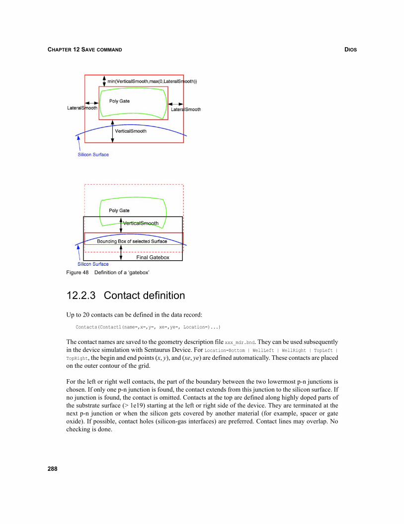
DIOSCHAPTER 12 SAVE COMMAND
Figure 48 Definition of a ‘gatebox’
12.2.3 Contact definition
Up to 20 contacts can be defined in the data record:
Contacts(Contact1(name=,x=,y=, xe=,ye=, Location=)...)
The contact names are saved to the geometry description file xxx_mdr.bnd. They can be used subsequentlyin the device simulation with Sentaurus Device. For Location=Bottom | WellLeft | WellRight | TopLeft |TopRight, the begin and end points (x, y), and (xe, ye) are defined automatically. These contacts are placedon the outer contour of the grid.
For the left or right well contacts, the part of the boundary between the two lowermost p-n junctions ischosen. If only one p-n junction is found, the contact extends from this junction to the silicon surface. Ifno junction is found, the contact is omitted. Contacts at the top are defined along highly doped parts ofthe substrate surface (> 1e19) starting at the left or right side of the device. They are terminated at thenext p-n junction or when the silicon gets covered by another material (for example, spacer or gateoxide). If possible, contact holes (silicon-gas interfaces) are preferred. Contact lines may overlap. Nochecking is done.
Final Gatebox
VerticalSmooth
288
DIOS CHAPTER 12 SAVE COMMAND
If all four coordinate parameters for a contact (x,y,xe,ye) are specified, a list of line segments is definedand added to the xxx_mdr.bnd file as a contact region. First, the line in the Dios layer system, closest tothe two specified points (x,y) and (xe,ye) is selected. This line is refined according to the parameters LMINand LMAX. The two Dios points, closest to the specified begin and end of the contact are kept but allinternal line segments are coarsened in the usual way. After coarsening, the line segments between thetwo points are defined as contact. Thus all line segments of one contact are on the same Dios line. Thisrestriction may lead to confusing selections of the contacts, since sometimes even the wrong line mightbe chosen.
If the end point (xe,ye) remains undefined, one of the Dios regions is renamed. The approximate position(x,y) of the midpoint of the bounding box of the region can be specified to select the region. If nomidpoint is specified, regions are renamed from right to left. Renaming is applied only to regions, whichconsist of a material that has been specified in Synonyms() to appear as metal in the file. By default this isperformed for AL, MS, Me, but for example, polysilicon regions can also be treated in this way:
Save(Synonyms(Po=Metal), Contacts(Contact1(Name=Gate,x=...,y=...Contact2(Name=Source,x=...,y=...)Contact3(Name=Drain,x=...,y=...)))
By default, the part of the boundary of renamed regions that is in contact to other selected regions willbe saved as a list of line segments. The default treatment of polysilicon depends on the selected meshingstrategy. For NewDiff=0 polysilicon is treated as metal. For NewDiff=1, polysilicon regions are saved withdoping by default. On the top part of the polysilicon, a contact can be placed, very similar to the contactthat is otherwise used for the boundary of regions, saved as metal. If the user defines Synonyms(Po=Metal),only the boundary of the polysilicon is saved as contact and no poly depletion can be simulated.
If an old format is used (that is, if a nonzero ISEFormat value is specified), the selected region is savedwith the material metal and replaced by its boundary line during the mesh generation in earlier Mdrawversions.
NOTE The contact definition in Dios is supposed to support simple standard cases only. For moreprecise and more complex contact definitions, the interactive mode of Mdraw must be used.Small metal or polysilicon areas may lead to strange contact name assignment.
NOTE The selected contacts cannot be displayed in Dios. Although the modified region names arekept during the subsequent Dios run, the material of a region in the Dios simulation is notaffected by Synonyms().
NOTE The coarsening does not change the Dios layer structure. The only change of thediscretization of the layer boundaries is performed by refining the selected lines around theend points of the contact lines.
289
DIOSCHAPTER 12 SAVE COMMAND
12.2.4 Command file
This section describes how the Dios input language can be used to define parameters for a Mdrawcommand file. The refinement sizes can be defined by the user; the placement of such refinements isperformed automatically by Dios, since the Mdraw command syntax does not offer automatic placementof refinement regions at, for example, the silicon surface at a gate. If possible, the same names of therefinement parameters are used as in the Mdraw command syntax. When saving files for the devicesimulation, a command file xxx_mdr.cmd (old: xxx.cmd) is generated by Dios, which contains referencesto the files with the Dios simulation grid and doping files, and which also contains refinementparameters. The global refinement parameters MaxElementWidth, MinElementWidth, MaxElementHeight,MinElementHeight, and MaxTransDiff can be specified in the Dios Save command. In addition, up to ten user-defined refinement boxes for Mdraw can be specified in the Dios Save command:
Save(Refinement( Box1(X Xe Y Ye MaxElementWidth MinElementWidth MaxElementHeight MinElementHeight MaxTransDiff) ... Box10(...)))
In the Save(Gate(...)) parameter record, a further set of refinement parameters can be specified. Therefinement regions in the silicon underneath the ‘gates’ are defined automatically by Dios. The lateralextension of these regions can be modified with the parameter LateralRefine. If LateralRefine is chosenequal to LateralSmooth, the refinement region and the ‘gateboxes’ are identical (see Figure 48 onpage 288). A series of small axis aligned refinement rectangles is saved into the Mdraw command filexxx_mdr.cmd. These rectangles try to capture the silicon surface underneath the gate. A series of verticalstepsizes MaxElementHeight and NumberOfIntervals can be specified in the Save(Gate(...)) parameterrecord to ensure a graded fine grid in the silicon underneath the gate. If VerticalSmooth=undefined isspecified, no ‘gate’ refinement is stored in the Mdraw command file. For strongly nonplanar ‘gate’surfaces (field oxide contour, trench) a larger value of VerticalSmooth might be required. In addition, alarge series of refinement rectangles will be produced to ‘outwit’ the axis-oriented refinement algorithmof Mdraw.
12.2.5 Grid and doping
The Dios simulation grid is saved in xxx_dio.grd[.gz] and the doping functions are saved inxxx_dio.dat[.gz] files. (old: xxx_dios.geo[.gz] and xxx_dios.dop[.gz]) The variables saved to the dat filecan be selected with SPecies(…). By default, the DATEX variables DopingConcentration (Dios: NetActive),TotalConcentration (Total) and the active (substitutional) concentrations for each of the dopants aresaved. If a germanium profile is defined during the process simulation and if in addition the userspecified Synonyms(SI=SG) the dataset XMolefraction will be saved for Sentaurus Device. All Diosvariables, which are not defined in DATEX, can only be saved as a dataset with the property Default.With Save(Type=DFISE) all Dios variables, known to Datex are saved into the file. Groups of species canbe selected by the user: Save(Species(AllTotal,AllActive,Net)).
NOTE The saving of DF–ISE files with the grid and data has been extended. Two types of savefunctions can be used in Dios.
290
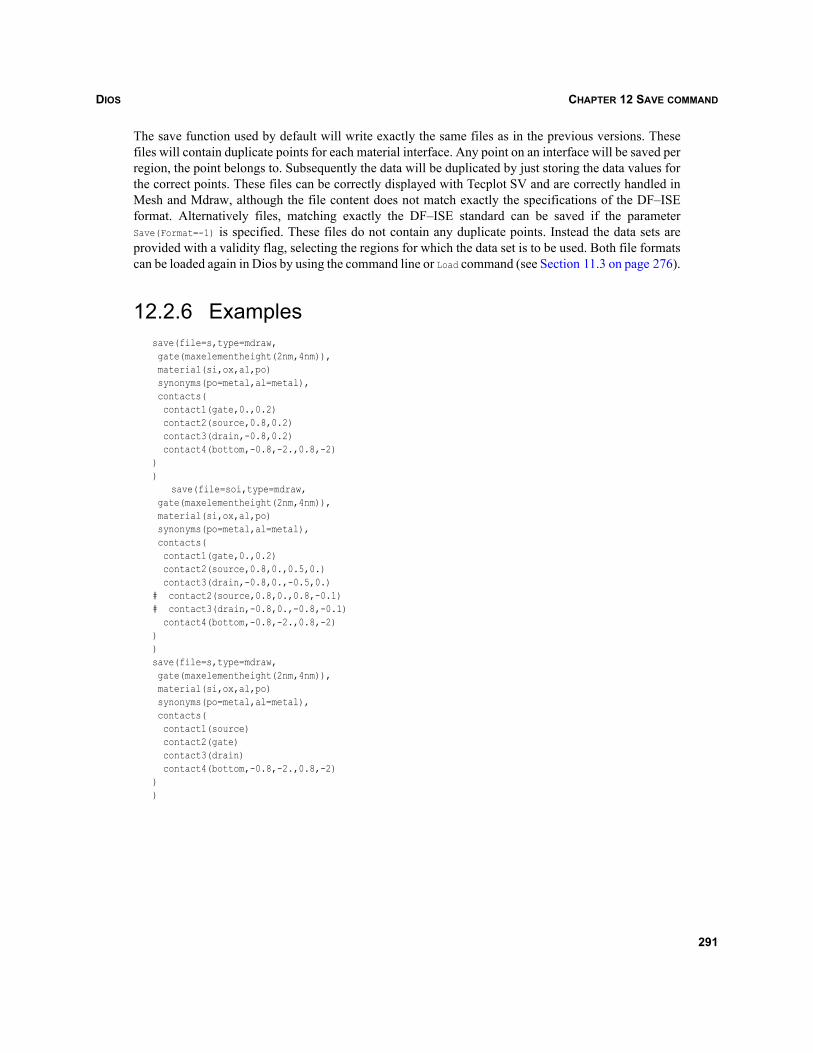
DIOS CHAPTER 12 SAVE COMMAND
The save function used by default will write exactly the same files as in the previous versions. Thesefiles will contain duplicate points for each material interface. Any point on an interface will be saved perregion, the point belongs to. Subsequently the data will be duplicated by just storing the data values forthe correct points. These files can be correctly displayed with Tecplot SV and are correctly handled inMesh and Mdraw, although the file content does not match exactly the specifications of the DF–ISEformat. Alternatively files, matching exactly the DF–ISE standard can be saved if the parameterSave(Format=-1) is specified. These files do not contain any duplicate points. Instead the data sets areprovided with a validity flag, selecting the regions for which the data set is to be used. Both file formatscan be loaded again in Dios by using the command line or Load command (see Section 11.3 on page 276).
12.2.6 Examplessave(file=s,type=mdraw, gate(maxelementheight(2nm,4nm)), material(si,ox,al,po) synonyms(po=metal,al=metal), contacts( contact1(gate,0.,0.2) contact2(source,0.8,0.2) contact3(drain,-0.8,0.2) contact4(bottom,-0.8,-2.,0.8,-2) ) )
save(file=soi,type=mdraw, gate(maxelementheight(2nm,4nm)), material(si,ox,al,po) synonyms(po=metal,al=metal), contacts( contact1(gate,0.,0.2) contact2(source,0.8,0.,0.5,0.) contact3(drain,-0.8,0.,-0.5,0.) # contact2(source,0.8,0.,0.8,-0.1) # contact3(drain,-0.8,0.,-0.8,-0.1) contact4(bottom,-0.8,-2.,0.8,-2) ) ) save(file=s,type=mdraw, gate(maxelementheight(2nm,4nm)), material(si,ox,al,po) synonyms(po=metal,al=metal), contacts( contact1(source) contact2(gate) contact3(drain) contact4(bottom,-0.8,-2.,0.8,-2) ) )
291
DIOSCHAPTER 12 SAVE COMMAND
12.3 Other file formatsThe file formats are selected with the parameter list Type. The following values can be specified:
dmp Binary or ASCII Dios file for subsequent continuation of the simulation ofevaluation of the results with Dios.
prf Two-dimensional doping profile (ASCII file, file content identical to exp). Thefunction diosi00 must be called to read the formatted file.
plf Formatted ‘snapshot’ file for the off-line coupling with the graphical programDegraf. Each ‘snapshot’ is written into a file. If APPend is specified, the‘snapshot’ is appended to an existing file. By default, only the layer structure iswritten into the file. If species are selected, the Dios grid and doping profile issaved too. Material() can be used to select the Dios materials to be saved.
exp Binary 2D doping profile. The variables can be selected with Species(). Thesefiles are used in the Reflect command and when saving point responses and as-implanted profiles during the simulation of ion implantation. If such files arecreated in the Save command, by default only NetActive and Total are saved intothe file. Such files can be used for an off-line link to external simulation tools.The Dios function diosi0 can be called to read the data file and the functiondiosi1 can be called for each point of the grid of the external tool, to interpolatethe doping values. In the past, this has been used as off-line interface to the 2Ddevice simulator TeSCA, distributed by WIAS Berlin. On request, the source filediosi0.F will be distributed.
dmp.gz A Dios save file is written and compressed using gzip -f. By default a binaryfile is created. If FORMAT=1, an ASCII file is created. The command sequence forthe call "gzip -f" can be specified as Replace(Control(GzipCall="...")). This isthe default type of file created in the Save command.
bound Formatted file, containing the layer structure, used for off-line coupling with thegrid generator Mdraw. By default a DF–ISE file with the extension _mdr.bnd isgenerated, for nonzero values of ISEFormat the old style files (ASCII bound file)is generated. After saving a file, a system call of the old bound2rand tool isperformed to translate the bound file into a binary rand file.
dp ASCII file containing doping profile in the PROETH file format. The doping isdefined in the bounding box of the substrate region. The doping is interpolatedto a tensor product grid with equidistant stepsizes in lateral resp. verticaldirections. The step sizes DXproeth and DYproeth or the number of discretizationpoints XProeth and YProeth can be prescribed, by default 50 nm spacing is used.If the lateral spacing is chosen larger than the width of the simulation domain,a 1D-PROETH file is written. The existing Total dopant concentrations AsTotal,BTotal, PTotal, SbTotal, and the Net doping are stored in the file.
cmd ASCII command file for Mdraw. Since the bounding box of the doping regionand the file names are written into the file, it must be created together with thedp, geo, and dop or _dio.grd.gz and _dio.dat.gz files.
292
DIOS CHAPTER 12 SAVE COMMAND
geb ASCII geometry description suitable for the grid generator trigen. The desiredmaximum and minimum edge lengths (LMAX LMIN) can be specified. In addition,concentration Levels(...) of the net doping can be specified, used for additionalsubdivisions of the layer structure. By default (DOTrect=on) the doping is writtenon a equidistant rectangular mesh, otherwise isolines for the net doping profileare stored into the file. The contacts can be specified by the location of start andend point and by the boundary type in the data record: BCtyp(Type1=...,
Xb1=...,Yb1=..., Xe1=..., Ye1=...). At most, 15 contacts can be specified.
MdrawAndLines Save files in Mdraw format and use a system call of mdraw -L to insert isolinesat a certain isoconcentration replace(control(Noffset(L1=... of the selectedspecies replace(control(Noffset(S1=... as multilines into the boundarydescription (see Section Q.2 on page 554).
dmp.Z A Dios save file is written and compressed. By default a binary file is created.If FORMAT=1 an ASCII file is created.
kg A Dios save file is written after a Use command that can be used for a transitionto TeSCA.
dom The UTRI grid is written in the dom format (see Section 4.3.1.5 on page 84).
MESHDp dp, bound, and cmd files are created.
lay The Dios layer system is written to an ASCII file (see Appendix U onpage 597).
lai The Dios layer system is written to a binary file (see Appendix U on page 597).
KPIF The Dios layer system, grid, and doping are written to an ASCII file, accordingto the Kyoko PIF standard.
meshbuild The _dio.grd[.gz], _dio.dat[.gz], _[parallel]_mdr.bnd, and _[parallel]_mdr.cmdfiles are written for later use in Mdraw. The _dio.grd[.gz] and _dio.dat[.gz]files contain the Dios grid and doping.
3D Save files after a 3D calculation.
Gip _gip.bnd, _dip.grd[.gz], and _dip.dat[.gz] are saved.
Mdraw _dio.grd[.gz], _dio.dat[.gz], _mdr.bnd and _mdr.cmd files are written for lateruse in Mdraw. The _dio.grd[.gz] and _dio.dat[.gz] files contain the Dios gridand doping. They are used in the submesh option of Mdraw and can bedisplayed using Mdraw or Tecplot SV. For nonzero values of ISEFormat the oldfile formats are saved: _dios.geo, _dios.dop, rand, bound, and cmd.
DF-ISE Geometry and doping concentrations are saved in _dio.grd[.gz] and_dio.dat[.gz] files in DF–ISE format.
293

DIOSCHAPTER 12 SAVE COMMAND
294
DIOS CHAPTER 13 GRAPHIC COMMAND
Dios
CHAPTER 13 Graphic command
13.1 OverviewIn the interactive mode, the command:
Graphic(
calls a local command loop, where graphical output can be performed. If the closing parenthesis isentered, the simulator leaves this local command loop. Graphic commands in the command files areexecuted. By default a 2D plot of layer system, net doping profile and p-n junctions (if present) areshown:
Graphic(Plot)
The pictures are drawn into a separate X11 window. The DISPLAY variable is checked:
setenv DISPLAY hostname:0.0
In batch mode (that is, when using the -b command-line flag), no X11 output is performed. Theexecution of command files is continued when the picture is finished. The parameter Wait (default 1)defines a waiting time between finishing the output and continuation of the simulation. For Wait=0, eachpicture has to be confirmed by pressing the Return key in the command/protocol window. Using Ctrl+C,cancels the drawing of the current picture. The selected species and parameters are kept if the Graphiccommand is left, such that for redrawing a similar picture the next time a short command is sufficient:Graphic(Plot), Graphic(Surface), or Graphic(Cross).
Replace(Control(NGraphic=10)) can be used to force Dios to redraw a picture every ten time steps and atthe end of each process step. Replace(Control(NGraphic=0)) switches off this mode and is the default.
Appendix L on page 515 lists the Graphic command parameters.
13.2 Event handlingIn 1D or 2D plots, you can zoom in and out. Moving the pointer while pressing the left mouse buttonselects a zoom region. If the button is released, a zoomed picture is drawn. To zoom out, click the zoomout button in the graphics window or click the middle mouse button. When clicking the redraw buttonor right-clicking, first an unzoomed 2D picture is drawn and, if this is repeated, the picture is switchedto 3D surface plot.
The current pointer position is used for sampling data or moving the zoom window in the device if theleft mouse button is clicked. You can switch the move button into the sample button and vice versa inthe graphics window. In the move mode, the pointer position is used as the new center of the (zoomed)picture and the picture is redrawn. In the sample mode, the coordinates corresponding to the pointer
295
DIOSCHAPTER 13 GRAPHIC COMMAND
position are printed in the command/output window. The length of the printout depends on the parameterINFO. In a 2D plot, in addition, the function values of all selected Species are printed. After clicking thespecies button, a new button is displayed for each of the available datasets. Click the appropriate one todisplay it. If you do not want to select one, click the species button again to hide the buttons for thedatasets.
The grid is displayed after clicking the triangle button. Clicking again hides the grid. The junctionbutton switches between Junction=Linear|No|Bezier beginning with Junction=Linear showing piecewiselinear p-n junctions.
Clicking the break button interrupts the computation. The button =/= switches between Scale(Equal=off)and the default Scale(Equal=on). The layer button switches betweenLayer=No|Contour|Material|Area|Line|Sort. The remaining options to display the layer system areavailable only in the interactive Dios input or in a command file. Different representations of the doping(Isoline=Fill|No|Isoline) can be toggled with the isoline button. The redraw button redisplays thepicture while keeping all actual graphics parameters unchanged. The exit button can be used to terminatethe Dios simulation. For safety reasons, this must be confirmed by clicking the confirm button. If theuser clicks somewhere else in the graphics window, exiting is not performed.
In a 2D plot, you can select the cutline of a 1D cross section by moving the pointer with pressing themiddle mouse button. After releasing the middle mouse button, a 1D cross section is drawn for allselected Species. If the cutline was outside the grid, it will be moved. The begin of the cutline (resp. thefirst intersection of the cutline and the grid) is used as the origin of the 1D plot and the distance alongthe cutline is displayed on the x-axis of the 1D plot. The length of the cutline, the thicknesses of theintersected material regions and the positions of the intersection points of the cutline and the materialinterfaces are printed in the command/output window. One can zoom in and out and move also in the1D cross section plots. The reset button can be used to first switch back to the unzoomed 1D view andif repeated to switch back to the 2D plot.
For a 3D surface plot, the Rotate and Tilt angles can be modified by moving the pointer with pressedmiddle mouse button (the same as a 1D cutline is selected in a 2D picture). The vertical extension of thedrawn line with respect to the window height defines the increment of TIlt and the lateral extension ofthe line relative to the window width defines the Rotate increment. With the reset button, you can firstreset the surface plot to the initial view and then switch back to the 2D view. No zooming is available inthe 3D view.
The picture is also redrawn if the user modifies the size of the X11 window. A full redraw of the picture,if the window was iconified or was partially hidden and is now visible unobscured, is done only if thecommand line parameter -redraw was specified when starting Dios or if the parameterGraphic(Window(Redraw=On))) is specified. Usually, the window manager should handle this redraw.
Since the simulation is continued, rigorously speaking, Dios cannot redraw a picture after the closingparenthesis was entered and the Graphic command was left. During the simulation, the X11 event queueis checked frequently if there are graphics events pending. A new picture can be drawn only when thisdoes not perturb the simulation (for example, at the end of a time step). Since it may take some time tostart the next drawing, the string redraw is printed to the command/output window if a redraw event hasbeen caught. The event queue is checked also, when commands are read from the keyboard. During thesimulation, the break button in the graphics window or Ctrl+C in the command/output window can be
296
DIOS CHAPTER 13 GRAPHIC COMMAND
used to interrupt the computation. At appropriate position Dios interrupts the simulation. In normalcommand execution mode, it enters the TControl( command mode. In this mode, Graphic and Printcommands can be used to analyze the structure, the grid or the doping functions. The simulation isstopped, but will be continued, when the closing parenthesis is entered or the go button in the graphicswindow is clicked in the TControl mode. The break and go toggle works also if Dios is used in SentaurusWorkbench mode (with the -u option). Since no command window is present in this case, no commandscan be typed in, and only the buttons in the X11 window can be used to analyze the structure and profiles.The simulation will resume only if the go button is clicked and the break button is displayed again.Button colors are used only to attract attention.
13.3 General parameters for all plotsThe variables to be displayed can be selected by Species(...). Dios variable names have to be used (seeSection 2.11 on page 72). Variables can be selected even before they are defined in the simulation but,of course, they are drawn only after they have been allocated in the simulation run. If no other variableis found, NetActive is drawn. A zoom region can be specified in the command file by:
Scale(XMid=..., YMid Factor=...)
or:
Scale(XLeft=...,XRight=...,YBottom=...,YTop=...)
SCale(Equal=on) is the default and ensures equal scaling of the x-axis and y-axis in the picture. The zoomregion is used for 1D, 2D, and 3D pictures, and also for the output in the Print and LControl commands.A zoom region defined by the user is kept until the user changes it. By default, the (changing in size)entire device is displayed.
Scale(Factor=1)
resets a user-defined zoom region. For Scale(Rescale=off), a fixed region is kept during the entiresimulation run. This can be used for comparison and especially for movies.
If ABS=on is specified, the absolute value of the selected functions is drawn in the 1D, 2D, and 3D pictures,respectively. If both components of a vector field are selected and if ABS=on is specified, isolines orisoareas of the norm of the vector field are displayed, rather than isoareas or isolines of the vectorcomponents.
If MIN or MAX is specified, the data and color range are restricted to the specified range.
CUT can be used to prescribe the minimum absolute value, displayed in the pictures. For each of thevariables, a linear, logarithmic, or hyperbolic transformation can be selected: LOGswitch(NetActive=Flog,AsTotal=Asinh, GrainShare=Linear). The color representation of the function values changes according tothe selected transformation. When zooming in and out, the color representation is adjusted to theminimum/maximum data range in the currently visible part of the device. The data legend is adjustedaccordingly.
297
DIOSCHAPTER 13 GRAPHIC COMMAND
13.4 Drawing 1D cross sections and other x-y plotsTo define vertical or lateral 1D cross sections, their lateral or vertical positions must be specified:XSection(...), YSection(...). Vertical cross sections are shifted by default to the local substrate surface(Shift=1e10) and are scaled from microns to nm (Factor=-1000). With XYSection(...), the start and endpoints of arbitrary straight cross sections can be prescribed. The cross section is displayed as a functionof the distance along the specified line. This is equivalent to the cross sections, selected with the mouse.For a 1D cross section plot, all intersection points of the specified cross section line and the triangleedges are computed. The function values of the selected Species are interpolated to these intersectionpoints. Some of the local variation in 1D profiles might result just from the position of the cuts in thetriangle and the interpolation. If all parameters (position, species) are defined, the cross sections arecomputed and drawn with the Cross command.
Arbitrary x-y plots can be read and displayed with the LinePlot command. A file name can be specified.A quite general (ASCII) file format is supported: all lines of the input file, which do not contain exactlytwo numbers, are interpreted as comment lines. A dataset is defined by a comment line and several datalines. Empty datasets are skipped. The first value of a data line is used as abscissa and the second asordinate. If the parameter Read=On is specified, all data sets of the file are read. Otherwise, the file is firstscanned, the comment lines are displayed and the datasets need to be selected interactively.
The NLinPlot command is used to redisplay x-y curves which are defined already (with maybe modifiedtransformation, selections or data range).
For XYPlot2D=On, these x-y plots are drawn onto a 2D picture when the Plot command is used (forexample, to show trajectories of MC implantation).
If Delete=off had been specified, the 1D cross sections are kept in memory, after they have beendisplayed. By default, all curves are removed and are recomputed for each redrawing operation. Whenusing Delete=on, NLinPlot all x-y curves are erased from the memory.
If Save=on is specified, the 1D cross sections and externally read curves are written to a File=... afterthey are drawn. The output file is in xgraph format.
13.5 Drawing 2D picturesTwo-dimensional pictures are drawn with the Plot command. The elements of the picture must beselected before using the Plot command: Isoline, Layer, Vector, Triangle, GLayer, Border, Junction,XYPlot2D. Materials, regions and boundary lines in which grid and doping are shown can be selected:Material(...) ISOMaterial(...) Area(...) Line(...). For Border=on, the outer contour line of the grid isdrawn. The parameter Isoline=No | OneByOne | AllInOne | SFill | Linked | Fill selects the drawing styleof isolines or isoareas. The default is Isoline=Fill on color displays and Isoline=OneByOne on black &white displays. The levels for the isoline and isoarea plot are chosen automatically, but can beoverwritten by the user:
Level(Species=...,NLevel=...,L1=...,L2=...)
298
DIOS CHAPTER 13 GRAPHIC COMMAND
The chosen levels are kept until the extremal values of the selected species in the zoom region arechanged by more than Level(ReSelect=100%). In this case the new extremal values are used to reselect thelevels automatically. If one wants to keep the color range and the displayed levels fixed, one shouldprescribe MIN, MAX and the levels as ZSCale(...). In this mode (for example, for movies), you have toknow or estimate the extremal values in advance.
Layer=No | Contour | Material | Area | Lines | Sort | FillMaterial | Line+Area | Zone | Line+Material
| Sort+Material | FillArea | Sort+Area selects different drawing styles of the layer system (that is, thepolygons). The parameter GLayer does the same for the regions in the grid.
Junction=Linear|No|Bezier selects different types of drawing the p-n junctions. The drawing forJunction=Bezier may take significant time, but provides smoothed curves. The line stylePNStyle=solid|bold|no defines the line style for the p-n junctions, PNMarker defines a marker for thejunctions. If both line PNStyle and PNMarker are set to No, the junctions are marked by filling the NetActiveprofile in the data range (-cut, cut) resp. (-1e9,1e9) with the color selected for the junction.
For Vector=on, vector valued functions are drawn as a vector field. At least one of the components of thevector must be selected as Species. If both vector components are selected, the x-component must bespecified first. If VSw=on, a vector is drawn in each grid point, otherwise VNX and VNY define an equidistantraster in the zoom region for which the values are interpolated and the vectors are drawn. For Grid=Itrionly VSw=on can be used. The lengths of the drawn arrows indicate the norm of the vector. By default, thelengths are scaled to the maximum of the norms of the displayed vectors, such that the arrows do notoverlap. The arrows can be scaled with a VFactor >1. A minimum relative length VMIN independent of thenorm can be used, to visualize the direction also for small vectors. For VMIN>VFactor, all arrows will havethe same length. By default VMIN=0.3 and VFactor=1.5. One may also prescribe the global maximum forthe norm VNOrm for all vector plots. In this case, all vectors are scaled with respect to this value. Thisallows to indicate a changing norm of the vectors in a series of pictures. Again the data range has to beknown in advance. A minimum value VSuppress can be prescribed to ensure, that no arrows are drawnfor data points where the norm of the vector is smaller than VSuppress. The parameter VSHape=-11, 0,11,12, 13, 14,... selects different style of the drawn arrows.
The parameter Triangle=On, selects drawing of the grid and the parameter Numbers=No | On | Diffusion |Poly | OXidation | All | Mechanics selects the drawing of node- and triangle numbers. The parameterGrid=On | Itri | Diffusion | USER selects the type of (intermediate) grid that is displayed. The default isGrid=On. For Grid=ITRI the various hierarchical refinement levels can be displayed: MLevel=1,...,10.
The command Value(X Y) prints the values for all selected Species interpolated for the given point. Inaddition, the numbers of the closest node and the triangle are printed (same as using ‘sample’ in thegraphics window).
13.6 Drawing 3D picturesThe command Surface can be used, to draw 3D hidden-surface plots of the selected species. By default,the functions are interpolated on a rectangular mesh. NST prescribes the maximum number of points inthis mesh. By default, a balanced spacing in x- and y-directions is assumed, but with MAXX and MAXY thelimits can be prescribed for each of the coordinate axes. The rotation and the tilt angle can beincremented Rotate=15, Tilt=-10, or the absolute values can be prescribed as RAngle, TAngle.
299
DIOSCHAPTER 13 GRAPHIC COMMAND
Alternatively, the coordinates of the view point VIEWX, VIEWY, VIEWZ can be specified. The parameter3Switch=Rectangle | Triangle | SRectangle selects different drawing algorithms. XName, YName and ZNameare the names of the coordinate axes that are displayed. XScale(...), YScale(...), ZScale(...) prescribethe values on the scale ticks.
13.7 Drawing multiple device views in X11 windowTo show several pictures in the Dios X11 window, first the picture size must be defined Window(Left RightBottom Top). Then, the picture is drawn with the Plot, Cross, Surface, and so on commands as usual. Thecurrent graphics parameter set is saved using the NextPicture() command. If the picture size for the nextpicture is not specified by the user, the largest non-overlapping rectangle is chosen by default. Thedescribed procedure may be repeatedly used.
The command DrawPicture() restores the saved parameter sets one after the other and redraws thepictures. If this command has been executed last before leaving the Graphic command, the automaticredrawing for example, with Replace(Control(NGraphic=1)) updates all pictures after each time step. Thecommand ErasePicture() deletes all saved parameter sets. The functions NextPicture, DrawPicture andErasePicture can be called with the number of a particular parameter set. In this case they handle just thespecified parameter set: DrawPicture(1). The default is 0, that is, handle all pictures.
NOTE Only the graphics parameters are saved and restored, not the grid, layer system, doping andso on. Thus, Dios does not allow to redraw different devices (for example, after loading twodmp files). The only way to avoid redrawing is to switch off the cleaning of the drawing area,and load and display the first picture in one part, and then to load and draw the second deviceand picture in another part of the window.
NOTE The usual operations such as zoom, reset, select cut, are not supported when drawing severalpictures.
13.8 Adding text, markers, lines, and arrowsAdditional text, markers, lines, and arrows can be drawn. By default, the file name of the loaded dmp fileor the text of the last comment is displayed. In general the text is stored as an array of strings Text(T1=...T10=...). If no comment is desired, Text can be reset to contain only empty strings, and/or an emptycomment can be entered outside of the Graphic command. The displayed coordinate system in a 1D or2D picture is used to position the text labels. In a 3D picture or when using the Label command, thepositions have to be defined in internal picture coordinates: (0…29.7) × (0…21). A vector of text strings,lateral and vertical positions and colors can be defined for the text.
TExt(T1='...',...,T10='...'), XText=(...), YText=(...), CText(...)
300
DIOS CHAPTER 13 GRAPHIC COMMAND
The parameter SText=Border | Plain | Background can be used, to change the style of the text labels. Formarkers and lines, a vector of lateral and vertical positions, colors and drawing styles can be defined:
XArrow(x1=10,y1=12) YArrow(y1=0 2) CArrow(c1=1), STarrow(s1=arrow)
The Label command just draws the specified text, markers and lines on top of the already drawn picture.Several attempts can be made to properly place the labels in the plot. When using the Plot, Cross, Surface,or Draw commands, the entire picture is redrawn and the last valid position is used for the labels.
13.9 Configuring X11 windowThe following entries in the window managers default file (for example, .X11defaults) are used:dios*Geometry, dios*Font, dios*Background. They can be overwritten by environment variables whichhave to be set, before Dios is started. The initial window size can be prescribed with the environmentvariable GMSSIZE (1: full screen, 2: 0.3 of the screen, 3: 0.8 of the screen). By default the graphics windowis 0.5 of the screen. The environment variable GMSWIDTH defines the line width in pixels.By default, sharedcolors are used. If Dios can not allocate enough shared colors on a color screen, it issues a warning andtries to create a private color map.
Parameters in the data record Window(...) control can be used to overwrite the defaults of the graphicalwindow during a running simulation. The size of the X11 window in relation to the screen width andheight can be specified with the parameters WSize, WHeight and the line width in pixels can be prescribedas Width. Left Right Bottom Top define the size and position of the next picture inside the window. LSHIFTand VSHIFT define an offset, reserved for scales. All these lengths are interpreted with respect to theinternal plot rectangle (0…29.7)×(0…21). By default, the entire window is used for the picture. Text isdrawn into the picture. The content of the color palette: materials MBox=on, species name and unit NBox=on,levels IBox, the position XBox, YBox and orientation Box=No | Lateral | UP | Horizontal | Down | UpOrLateralcan be specified. By default, the palette is placed UpOrLateral, wherever it fits best.
The parameter Clear=PlotArea | No | Window | OnceWindow | Border | NewWindow | Destroy can be used tocontrol the behavior of the graphics window, when the next picture is drawn. Sometimes for example,Clear=No is helpful, for example, to compare the evolution of etching fronts with layer=line or of 1Dprofiles in Cross.
If the user specifies Words=on, the drawing region is subdivided into a picture and a text part. PLeft,PRight, PBottom and PTop define the picture part. 2D pictures are drawn in the right or bottom part. Thetext is drawn in the left or upper side. PLeft and PTop prescribe the used picture range, DLeft and DTop areused as defaults. TTop and TLeft locate the text window, LPos=Centered | Left | Right and VPos=Centered| Bottom | Top are used, to place the simulation domain in the picture part. By default WORDs=off and allthese parameters are ignored.
In Dios, only a single X11 font is used. An appropriate line in the .X11defaults file: dios*Font:cour.b.16or an environment variable: setenv GMSFONT "-adobe-courier-bold-r-normal–25-*-100-*-*-*-*-*" or theparameter FONT='screen.b.16' in the Window data record can be specified. If no font is specified, the defaultfont in the X11 server is used. The character and line spacing is adjusted automatically. If necessary, theparameters ZLine, ZSize, and ZDist can be used for the fine tuning. ZLine defines the line spacing and ZSize
301
DIOSCHAPTER 13 GRAPHIC COMMAND
the character height and the offset of an exponent with respect to the internal plot range (0…21). ZDistdefines the lateral spacing of the characters with respect to (0…29.7).
High, DotLow, LineLow, and Bold define the lengths and the thicknesses for the various line styles. If the fontor the size of the graphical window are changed, these parameters might have to be adjusted.
13.10 Selecting colorsColors can be defined in the data record Colors. The parameters Substrate=on and Gas=on control thepolygon filling of the substrate and the gas regions when drawing the layer system. Color indices can begiven for Scales, Text, Triangle, triangle and node numbers TriangleNumber, NodeNumber, contour lines inthe layer system plot LayerSystem, the outer contour of the simulation domain Border, vectors Vector andVector1, p-n junctions PNColor, and the top and bottom side of a 3D plot SuTop and SuBottom.
The color indices for each Material(), the triangles in the material TriMaterial(), and the boundary sortSort() can be defined also. Area(Area Color=...) and Line(Line Color=...) can be used to highlight acertain region or line. If the color index Logo is defined, the text string specified as Window(Logo='...')isdrawn. If it is undefined, a color ball is drawn; if it is set –1 (default), no logo is drawn. The fourparameter vectors Index(), Red(), Green(), and Blue() can be used to redefine the RGB values for thespecified color indices.
Index 0 is used for the background color (white: Red=255 Green=255 Blue=255). Index 1 defines the inverse(black: Red=0 Green=0 Blue=0). The color indices 1…7 (black, red, green, blue, yellow, magenta, cyan)are used for grid, scales, text, contacts, surface plots, and so on. If necessary, they are repeatedly used.The next group of color indices are preserved for displaying the materials in the layer system plot. Thecolors for the materials are defined in the datexcodes.txt file and are shared by all Synopsys TCAD tools.
The remaining colors in Dios are used as a rainbow to indicate the function values in the 2D plots. Diosuses a total of 50 colors. To modify a color, the index and RGB values must be specified. Steps definesthe number of color levels in the isoline/isoarea plot. For Steps=2 in the net doping, only n- and p-regionsare distinguished (red and blue). If Steps is larger than the number of allocated colors, all colors from therainbow are used. The levels in the palette are drawn each in a single color. This is the default. Forsmaller values of STeps, the line of change of the color defines the isoline to the specified level.
13.11 Saving pictures as graphic filesDios pictures can be saved as HPGL plotter files hpgl, Encapsulated PostScript files eps, Sun raster filesras, or GIF files gif. This can be selected with the parameter Terminal=PS | HPGL | ras | ras.Z | ras.gz| gif | gif.Z.
For the raster and GIF file formats, first the normal X11 picture is drawn and the following UNIXcommands are used to save the files:
xwd -name ...|xwdtopnm|pnmtorastxwd -name ...|xwdtopnm|ppmtogif
302
DIOS CHAPTER 13 GRAPHIC COMMAND
Users must ensure that these public domain tools are available in the path. Otherwise, they can use theparameters GIFCMD resp. RASCMD to specify an appropriate UNIX command. The Terminal is modified justfor one picture and then reset to the default Terminal=X11.
The drivers for PostScript and HPGL are implemented directly in Dios. After selecting Terminal=PS andthen executing a Plot, Cross, or Surface command, the X11 window disappears and a similar picture isdrawn using the PostScript or HPGL driver. After saving the picture, the user should switch toTerminal=X11. Otherwise, all subsequent pictures are written to a further file also.
Dios can be used to save a series of similar pictures as a movie: Movie=ras | ras.Z | ras.gz | gif | gif.Z| gif.gz. The command sequence to show the ‘movie’ is written into a file with the extension xmovie.After the Dios simulation is performed, the movies can be displayed using: xmovie xxx.xmovie. A secondcommand file, using screenload commands is written into an executable shell script with the extensionmovie. The name of the movie files can be specified.
Some ‘extras’ may be useful in the movies. An analog watch can be drawn to illustrate the totalprocessing time: CLock(Xmid=..., Ymid=..., XDiameter=..., YDiameter=...).
The temperature can be displayed: Temperature(Xleft Ybottom), or a diagram can be used to show thecurrent process step time and the temperature profile: Clock(StGone=Difbar).
303

DIOSCHAPTER 13 GRAPHIC COMMAND
304
DIOS CHAPTER 14 1D COMMAND
Dios
CHAPTER 14 1D command
14.1 OverviewThe 1D command is used to save 1D cross sections into a file, for example, for comparison with 1Dsimulations or SIMS profiles. The cross sections can be chosen along the vertical or lateral directions,or they can follow an arbitrary straight line. Appendix M on page 543 lists the 1D command parameters.
By default, the 1D cross sections are saved as plx files suitable for the public domain tool XGRAPH. If1d(file format=mdraw) is specified, the comment lines are chosen in a special way such that the files canbe used in Mdraw. If Format=XMGR, an appropriate format is saved and the names of the species are printedto the protocol to be used for the labels in XMGR.
If PIntegral=on is specified, the integral and the moments of the 1D cross sections are printed.
If RS=on is specified, the sheet resistance in of entire semiconductor layers or between neighboringp-n junctions along the selected 1D cross section is printed instead. The resistivity is computed from theactive concentrations at the most recent process temperature. If no active concentrations are present, thetotal concentrations are used instead. The electron and hole concentrations are defined assuming avanishing space charge and recombination equilibrium for a device temperature of 300 K. The intrinsiccarrier density is computed according to Eq. 213. From the dopant concentrations, the electron and holemobilities at the device temperature are defined. Only constant and doping dependent mobilities areconsidered. Any other dependency for example, on the electric field is neglected. The implementedmodels [3][13][37] are valid for crystalline silicon at device temperatures of about 300 K.
A modified mobility model is used for polycrystalline materials. The mobility depends on thepolysilicon grain size. Two parameters have been added, describing the surface density of trap centersand their energy:
diff(po(QT0=.../cm2, AWT=...eV))
The model is similar to the one used in the 1D simulator TESIM-4. It provides qualitatively correctresults but the absolute value for polysilicon is rather difficult to predict. Differences to TESIM-4 maybe explained by different model assumptions, since in Dios the grain boundary concentration areassumed electrically neutral (consistently in the diffusion and in the calculation of net profile, spacecharge and RS computation). Differences in the grain growth model may also contribute.
Ω/
305
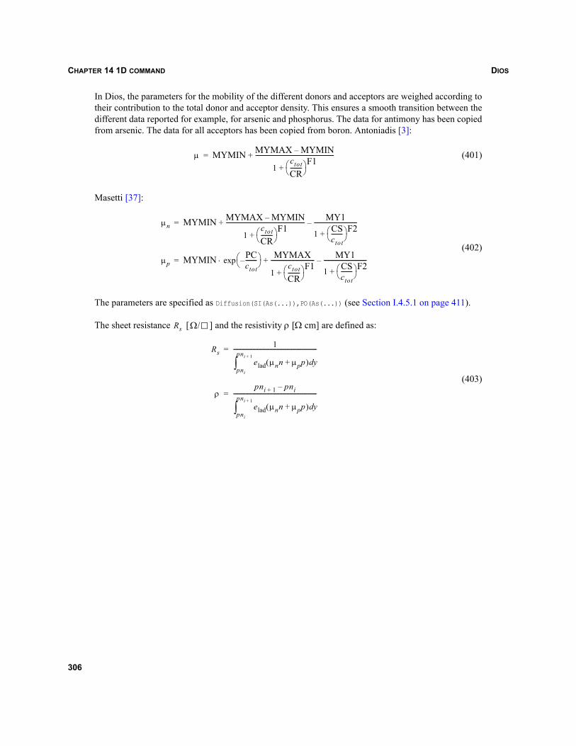
DIOSCHAPTER 14 1D COMMAND
In Dios, the parameters for the mobility of the different donors and acceptors are weighed according totheir contribution to the total donor and acceptor density. This ensures a smooth transition between thedifferent data reported for example, for arsenic and phosphorus. The data for antimony has been copiedfrom arsenic. The data for all acceptors has been copied from boron. Antoniadis [3]:
(401)
Masetti [37]:
(402)
The parameters are specified as Diffusion(SI(As(...)),PO(As(...)) (see Section I.4.5.1 on page 411).
The sheet resistance [ ] and the resistivity ρ [Ω cm] are defined as:
(403)
μ MYMIN MYMAX MYMIN–
1ctotCR--------⎝ ⎠
⎛ ⎞ F1+
--------------------------------------------------------+=
μn MYMIN MYMAX MYMIN–
1ctotCR--------⎝ ⎠
⎛ ⎞ F1+
-------------------------------------------------------- MY1
1 CSctot--------⎝ ⎠
⎛ ⎞ F2+------------------------------–+=
μp MYMIN PCctot--------–⎝ ⎠
⎛ ⎞exp⋅ MYMAX
1ctotCR--------⎝ ⎠
⎛ ⎞ F1+
------------------------------- MY1
1 CSctot--------⎝ ⎠
⎛ ⎞ F2+------------------------------–+=
Rs Ω/
Rs1
elad μnn μpp+( ) ydpni
pni 1+
∫-----------------------------------------------------------=
ρpni 1+ pni–
elad μnn μpp+( ) ydpni
pni 1+
∫-----------------------------------------------------------=
306
DIOS CHAPTER 15 PRINT
Dios
CHAPTER 15 Print
15.1 OverviewThe length of the Dios protocol is defined by the parameters LProt, IPRNwt, and Info in the parameterrecord Control. They are usually specified with the Replace command for the entire simulation:
Replace(Control(LProt=2,IPRNwt=2,Info=1))
During the diffusion steps, the current process time, temperature, time step and end time of the process,the oxide thickness resp. maximum velocities are printed if LProt=1. For LProt=2 in addition, the integraland the extremal values of the doping are printed. LProt=0 switches off this output and is the default. Ifthe parameter IPRNwt=2 is chosen, the full information about the newton iteration is printed. This shouldbe checked, if convergence problems are detected. The number of Newton iterations xxx.it, the speciesname, the norm of the initial guess |x|=..., the norm of the Newton increments |dx|/|x|=… and the normof the right hand side (defect) |rhs|=... are printed for each iteration. The factor of desired reduction of|rhs| compared to the maximum value during the iteration (DEFReduction) and the required value of |dx|/|x| (Errnwt) are checked if the solution is to be accepted.
solv=... describes the number of inner iterations for an iterative linear solver. The maximum isprescribed by ITLin. If a direct solver is used, always solv=1 is printed.
The relative defect reduction of the linear solver (norm of final defect, divided by norm of initial defect,that is, |rhs-A*dx|/|rhs|) is printed in the last column, the desired reduction can be specified as DEFLin.If the maximum number of linear iterations has been performed, but the relative defect still exceeds DEFA,the solution of the linear system is rejected and either the time step or the solver program is changed.
If an equation was not solved during an iteration, solv=skipped is printed. An ‘m’ in the solver printoutindicates that a new matrix has been assembled (and factorized).
For IPRNwt=1, only the last Newton iteration is printed. For IPRNwt=0, this printout is switched off.
The process step data is printed for Info<0. For larger values of Info, more and more test prints areactivated. Info controls the output to the terminal and the output to the protocol file.
307

DIOSCHAPTER 15 PRINT
15.2 Print commandThe Print command is used to insert additional printed information about the layer structure, topology,datasets, or process step data into the protocol file.
Appendix N on page 545 lists the Print command parameters.
If the parameter NPrint=10 in the Control record is specified, the last Print command is repeated aftereach ten time steps and at the end of each process step. The Print command can be used also in theTControl mode (after using Ctrl+C or clicking the break button in the graphics window). The printedoutput can be redirected (temporarily) to a different file:
Print(Protocol='name',Append=on|off)
308
DIOS CHAPTER 16 MEASURE COMMAND
Dios
CHAPTER 16 Measure command
16.1 OverviewThe Measure command in Dios is used to extract any data from the log file into the parameter table ofSentaurus Workbench. Before inserting a Measure command, the required printed output must beenforced, for example, by inserting Print or 1D commands. There is no restriction to the information thatcan be measured, for example, dose versus time. The only requirement is a unique piece of prototypelog file from Dios that can be transformed into a template. This is performed easily by replacing thenumbers and other free data by named parameters of Sentaurus Workbench. Appendix O on page 549lists the Measure command parameters.
When using the template, it is necessary to specify the template name and a list of pairs of such symbolicnames, and names under which the extracted values are to be stored in the Sentaurus Workbench table.The extracted values are entered into the Sentaurus Workbench table only after the execution of Dios isfinished. During the execution of the Dios Measure command, a system call of the Measure tool isperformed. The creation of templates and the regular expression syntax of Tcl/Tk is described inUtilities, Chapter 7 on page 59. The Dios Measure command can be used if all the information that is beextracted has been printed already into the Dios protocol file:
Measure(Template=thres,LabelAndName("m1","Rs","uSurf","Surface"))Measure(Command=n17_ms1.cmd)
Started from inside Dios, the Measure tool analyses the actual Dios protocol file. Using the giventemplate, Measure scans the protocol file, collects the values from the positions given by the labelpositions, and prints the values with the specified names into the Dios protocol file as:
DOE: Surface 0.007DOE: Rs 3383.6
A comment line:
### measure call: 1 ###
is added to the Dios protocol file (the number counts the measure calls) in order to prevent Measure,during its next run in the same process flow, extracting again the parameters from a preceding Measurecall.
309

DIOSCHAPTER 16 MEASURE COMMAND
310
DIOS CHAPTER 17 REFLECT COMMAND
Dios
CHAPTER 17 Reflect command
17.1 OverviewWith Dios, only half of a symmetric structure can be simulated. The Reflect command is used to expand,shrink, shift, or reflect the layer structure, the grid, the functions defined on the grid and, if possible, therefinement rectangles. The symmetry line must be at the left or right boundary or outside of the structure,resp. the chosen window. If the reflect line is outside of the existing structure, an 1D part is inserted, forexample, the gate length is ‘stretched.’ Appendix R on page 589 lists the Reflect command parameters.
The Reflect command can be used repeatedly, but only one reflection at either the left or right side isallowed per Reflect command. It may be necessary to apply the command several times to avoidambiguous situations. Lateral and vertical 1D continuation resp. reflection are applied to the profiles, noextrapolation is performed.
Besides reflection, a structure can be stretched at a certain x-location (Xloc) to the right by using theparameters in the Reflect(Stretch( record. Here, Xloc determines where to cut the structure and Lengthdetermines how far the structure is ‘stretched’ to the right. Profiles in the newly generated region aregiven by the profile at the cutline:
Reflect(Stretch(Xloc=1um Length=0.5um))
The above command extends a given structure at position x=1 μm by 0.5 μm to the right. Xloc has to beinside of the initial structure.
A ‘combination’ of several Dios layer structures is not foreseen in the Reflect command. This must beperformed in Mdraw or by using the LControl command (see Appendix U on page 597). Of course,analytic profiles can be loaded after using the Reflect command to expand the Dios structure and grid:
Reflect(Window(Left Right Top Bottom=...),Reflect Shift VShift=...
)
During the Reflect command, the layer structure is reflected exactly. The user-defined refinement boxesare ‘reflected’ and the grid parameters are adjusted. Usually, a new grid is generated, starting with anadjusted user grid and performing a complete mesh adaptation.
311
DIOSCHAPTER 17 REFLECT COMMAND
NOTE A nonsymmetry in the final mesh after the reflection may be caused by the intersection of thefinal mesh adaptation tree with the (original plus reflected) material boundaries. Thisoperation does not respect any symmetry or periodicity of the structure. Due to round-offerrors, in rare cases, even the interpolated data may become nonsymmetric. The reason forthis is mainly a poor mesh quality in the mesh just before the reflection. The user can adjustthis.
An algorithm implemented in the Reflect command can be used to exactly shift, vshift, or reflect asimulation grid. The exact shift or reflection of the mesh is selected if the commandReplace(Control(ConvertGrid=1)) is executed before the Reflect command.
This type of the reflect command can be used to generate exactly symmetric meshes. Obviously, thereflection can only be performed if the reflect line is exactly on the left or right side of the existingdevice.
NOTE Any change of the layer structure or an explicit Adap() command resets ConvertGrid=0.
In the case of interpolation errors during the normal mesh adaptation, this ‘mesh reflection’ can be usefulsince no data interpolation is involved at all. The ‘mesh reflection’ can be useful also at the very end ofa process simulation when saving data for external meshing tools.
For the reflection of the grid before, for example, a Monte Carlo halo implantation, the reflection of themesh is not recommended, since the grid needs to be expanded at the left and right symmetry lines toprevent the decay of the profiles at the left and right sides of the domain.
Dios offers the possibility to handle the rear side of a structure. The Reflect(FlipY=...) command can beused to reflect the structure about the x-axis. When extracting the layer structure on the new top of thestructure, a gas region is added. Oxidation processes are always handled on top and bottom.Implantation, deposition, etching, and masking are applied always to the top gas region.
NOTE The second gas region does not disappear during simulation steps.
312
DIOS CHAPTER 18 ADVANCED CALIBRATION
Dios
CHAPTER 18 Advanced Calibration
18.1 OverviewSynopsys Simulation & Services has been working continually on improving the simulation models andoptimizing the model parameters for the latest technology nodes. This effort is based on a long-standingexperience of model calibration for customers and a comprehensive, growing database of state-of-the-art secondary ion mass spectroscopy (SIMS) profiles. Advanced Calibration provides users with a set ofparameters that have been calibrated to deep submicron CMOS technology.
With these parameters, the accuracy of Dios simulation results is significantly improved for manyprocesses in device fabrication such as ion implantation, ultrashallow junction (USJ) formation, surfacedose loss, and channel and halo dopant diffusion.
The Dios Advanced Calibration is contained in parameter files, named AdvCal_1d_tables_2005.10.dmr,AdvCal_1d_CTRIM_2005.10.dmr, AdvCal_2d_nMOS_2005.10.dmr, AdvCal_2d_pMOS_2005.10.dmr, and located in thedirectory $STROOT/tcad/$STRELEASE/lib/dioslib. These files contain a selection of physical models andparameters. Using the Merger application, they can be merged with a Dios input file, which containsonly the pure process flow without any choice of physical models and parameters.
For comprehensive documentation of the Dios Advanced Calibration, refer to the Advanced CalibrationUser Guide. It describes:
How to use the Dios Advanced Calibration.
The contents of the Dios Advanced Calibration files. All models and parameters are explained.
The calibration method and the limitations of the Dios Advanced Calibration.
How to use the Merger application. Merger offers the most efficient way of using the Dios AdvancedCalibration files.
The Advanced Calibration files are a good starting point for a 2D calibration, especially for deepsubmicron CMOS technology. These files can significantly reduce the effort for 2D calibration, butcannot replace it. TCAD users can fine-tune the parameters, for example, to improve the agreementbetween their experimental data and the simulation results in a certain process condition window. Forthis purpose, users can copy the Advanced Calibration files into their own directory and makeappropriate changes. For an efficient and physics-based recalibration, it is recommended that users readthe information provided in the Advanced Calibration documentation. A customized calibration ofprocess and device simulation models can be requested from Synopsys in the context of customerservice projects.
313

DIOSCHAPTER 18 ADVANCED CALIBRATION
314
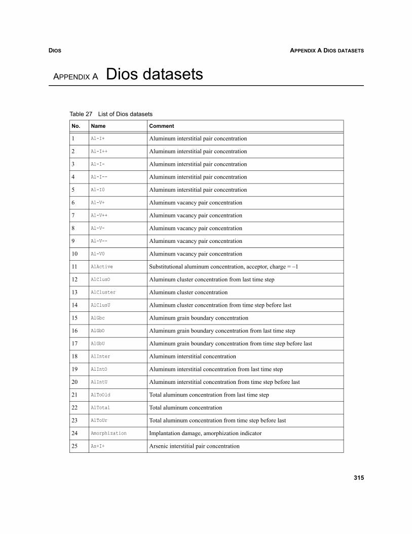
DIOS APPENDIX A DIOS DATASETS
Dios
APPENDIX A Dios datasets
Table 27 List of Dios datasets
No. Name Comment
1 Al-I+ Aluminum interstitial pair concentration
2 Al-I++ Aluminum interstitial pair concentration
3 Al-I- Aluminum interstitial pair concentration
4 Al-I-- Aluminum interstitial pair concentration
5 Al-I0 Aluminum interstitial pair concentration
6 Al-V+ Aluminum vacancy pair concentration
7 Al-V++ Aluminum vacancy pair concentration
8 Al-V- Aluminum vacancy pair concentration
9 Al-V-- Aluminum vacancy pair concentration
10 Al-V0 Aluminum vacancy pair concentration
11 AlActive Substitutional aluminum concentration, acceptor, charge = –1
12 AlClusO Aluminum cluster concentration from last time step
13 AlCluster Aluminum cluster concentration
14 AlClusU Aluminum cluster concentration from time step before last
15 AlGbc Aluminum grain boundary concentration
16 AlGbO Aluminum grain boundary concentration from last time step
17 AlGbU Aluminum grain boundary concentration from time step before last
18 AlInter Aluminum interstitial concentration
19 AlIntO Aluminum interstitial concentration from last time step
20 AlIntU Aluminum interstitial concentration from time step before last
21 AlToOld Total aluminum concentration from last time step
22 AlTotal Total aluminum concentration
23 AlToUr Total aluminum concentration from time step before last
24 Amorphization Implantation damage, amorphization indicator
25 As+I+ Arsenic interstitial pair concentration
315
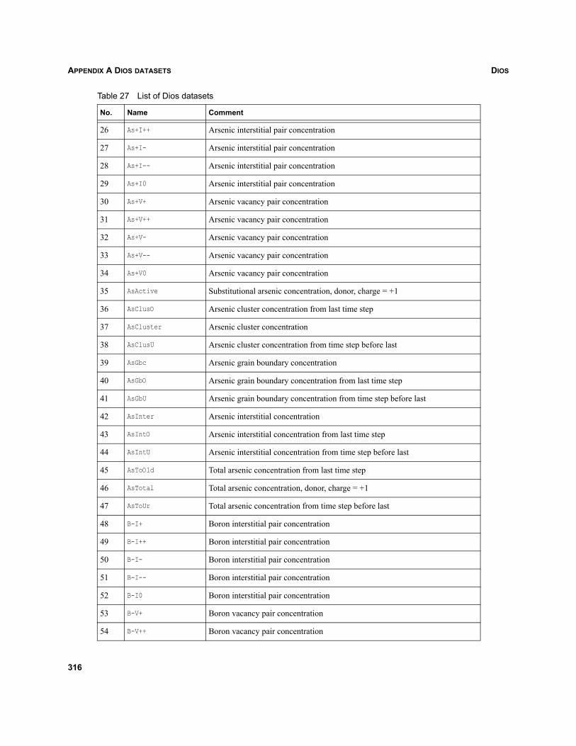
DIOSAPPENDIX A DIOS DATASETS
26 As+I++ Arsenic interstitial pair concentration
27 As+I- Arsenic interstitial pair concentration
28 As+I-- Arsenic interstitial pair concentration
29 As+I0 Arsenic interstitial pair concentration
30 As+V+ Arsenic vacancy pair concentration
31 As+V++ Arsenic vacancy pair concentration
32 As+V- Arsenic vacancy pair concentration
33 As+V-- Arsenic vacancy pair concentration
34 As+V0 Arsenic vacancy pair concentration
35 AsActive Substitutional arsenic concentration, donor, charge = +1
36 AsClusO Arsenic cluster concentration from last time step
37 AsCluster Arsenic cluster concentration
38 AsClusU Arsenic cluster concentration from time step before last
39 AsGbc Arsenic grain boundary concentration
40 AsGbO Arsenic grain boundary concentration from last time step
41 AsGbU Arsenic grain boundary concentration from time step before last
42 AsInter Arsenic interstitial concentration
43 AsIntO Arsenic interstitial concentration from last time step
44 AsIntU Arsenic interstitial concentration from time step before last
45 AsToOld Total arsenic concentration from last time step
46 AsTotal Total arsenic concentration, donor, charge = +1
47 AsToUr Total arsenic concentration from time step before last
48 B-I+ Boron interstitial pair concentration
49 B-I++ Boron interstitial pair concentration
50 B-I- Boron interstitial pair concentration
51 B-I-- Boron interstitial pair concentration
52 B-I0 Boron interstitial pair concentration
53 B-V+ Boron vacancy pair concentration
54 B-V++ Boron vacancy pair concentration
Table 27 List of Dios datasets
No. Name Comment
316
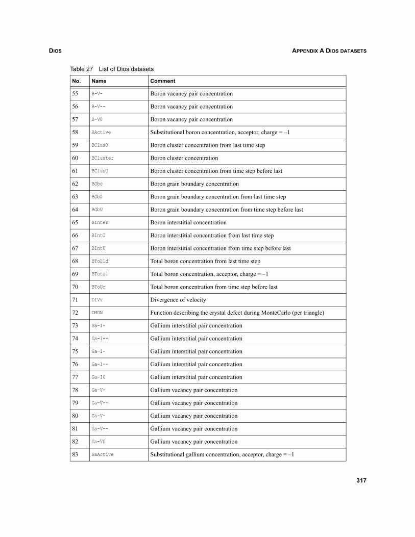
DIOS APPENDIX A DIOS DATASETS
55 B-V- Boron vacancy pair concentration
56 B-V-- Boron vacancy pair concentration
57 B-V0 Boron vacancy pair concentration
58 BActive Substitutional boron concentration, acceptor, charge = –1
59 BClusO Boron cluster concentration from last time step
60 BCluster Boron cluster concentration
61 BClusU Boron cluster concentration from time step before last
62 BGbc Boron grain boundary concentration
63 BGbO Boron grain boundary concentration from last time step
64 BGbU Boron grain boundary concentration from time step before last
65 BInter Boron interstitial concentration
66 BIntO Boron interstitial concentration from last time step
67 BIntU Boron interstitial concentration from time step before last
68 BToOld Total boron concentration from last time step
69 BTotal Total boron concentration, acceptor, charge = –1
70 BToUr Total boron concentration from time step before last
71 DIVv Divergence of velocity
72 DMGN Function describing the crystal defect during MonteCarlo (per triangle)
73 Ga-I+ Gallium interstitial pair concentration
74 Ga-I++ Gallium interstitial pair concentration
75 Ga-I- Gallium interstitial pair concentration
76 Ga-I-- Gallium interstitial pair concentration
77 Ga-I0 Gallium interstitial pair concentration
78 Ga-V+ Gallium vacancy pair concentration
79 Ga-V++ Gallium vacancy pair concentration
80 Ga-V- Gallium vacancy pair concentration
81 Ga-V-- Gallium vacancy pair concentration
82 Ga-V0 Gallium vacancy pair concentration
83 GaActive Substitutional gallium concentration, acceptor, charge = –1
Table 27 List of Dios datasets
No. Name Comment
317
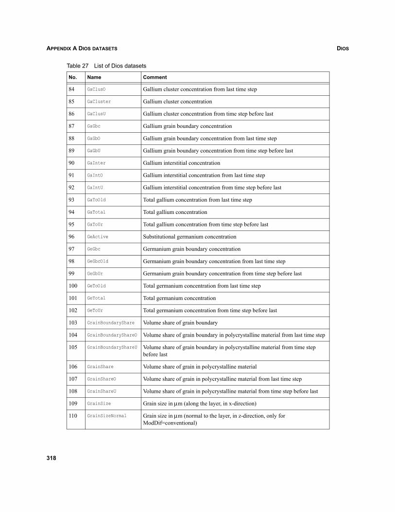
DIOSAPPENDIX A DIOS DATASETS
84 GaClusO Gallium cluster concentration from last time step
85 GaCluster Gallium cluster concentration
86 GaClusU Gallium cluster concentration from time step before last
87 GaGbc Gallium grain boundary concentration
88 GaGbO Gallium grain boundary concentration from last time step
89 GaGbU Gallium grain boundary concentration from time step before last
90 GaInter Gallium interstitial concentration
91 GaIntO Gallium interstitial concentration from last time step
92 GaIntU Gallium interstitial concentration from time step before last
93 GaToOld Total gallium concentration from last time step
94 GaTotal Total gallium concentration
95 GaToUr Total gallium concentration from time step before last
96 GeActive Substitutional germanium concentration
97 GeGbc Germanium grain boundary concentration
98 GeGbcOld Germanium grain boundary concentration from last time step
99 GeGbUr Germanium grain boundary concentration from time step before last
100 GeToOld Total germanium concentration from last time step
101 GeTotal Total germanium concentration
102 GeToUr Total germanium concentration from time step before last
103 GrainBoundaryShare Volume share of grain boundary
104 GrainBoundaryShareO Volume share of grain boundary in polycrystalline material from last time step
105 GrainBoundaryShareU Volume share of grain boundary in polycrystalline material from time step before last
106 GrainShare Volume share of grain in polycrystalline material
107 GrainShareO Volume share of grain in polycrystalline material from last time step
108 GrainShareU Volume share of grain in polycrystalline material from time step before last
109 GrainSize Grain size in μm (along the layer, in x-direction)
110 GrainSizeNormal Grain size in μm (normal to the layer, in z-direction, only for ModDif=conventional)
Table 27 List of Dios datasets
No. Name Comment
318
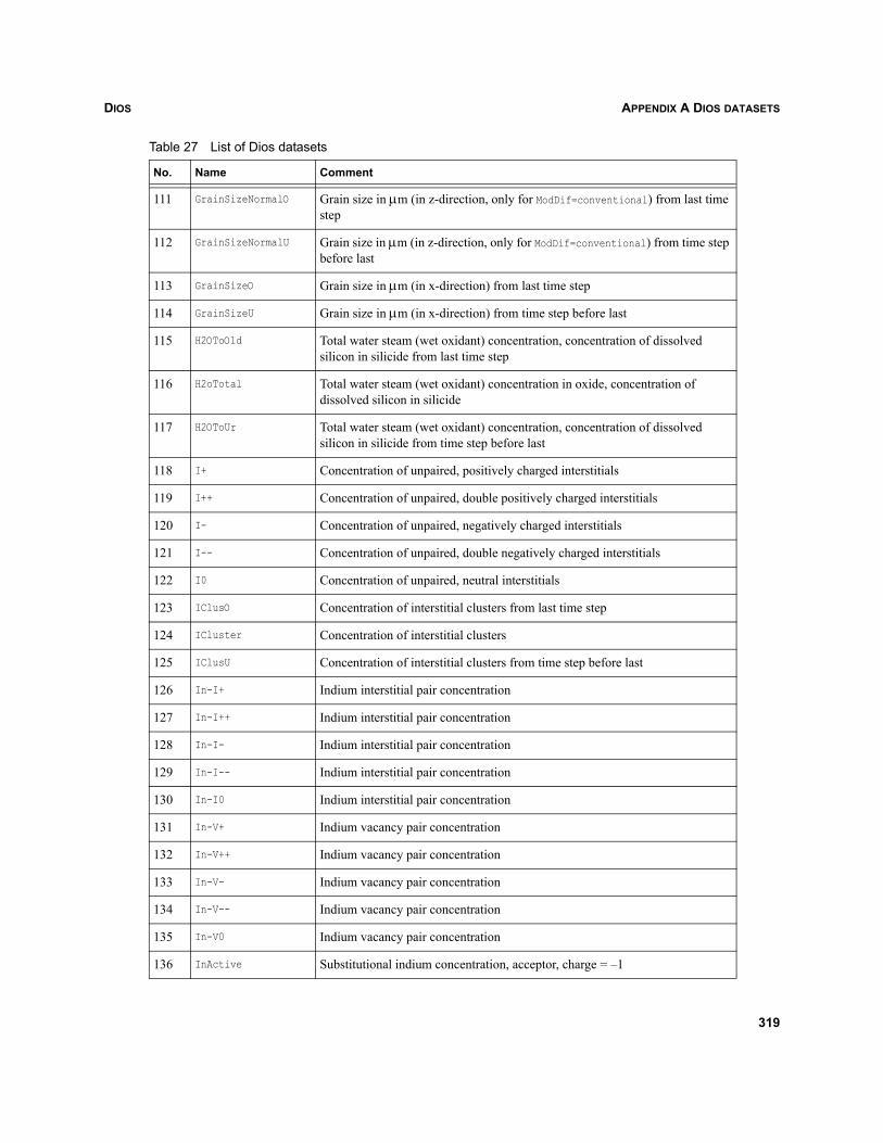
DIOS APPENDIX A DIOS DATASETS
111 GrainSizeNormalO Grain size in μm (in z-direction, only for ModDif=conventional) from last time step
112 GrainSizeNormalU Grain size in μm (in z-direction, only for ModDif=conventional) from time step before last
113 GrainSizeO Grain size in μm (in x-direction) from last time step
114 GrainSizeU Grain size in μm (in x-direction) from time step before last
115 H2OToOld Total water steam (wet oxidant) concentration, concentration of dissolved silicon in silicide from last time step
116 H2oTotal Total water steam (wet oxidant) concentration in oxide, concentration of dissolved silicon in silicide
117 H2OToUr Total water steam (wet oxidant) concentration, concentration of dissolved silicon in silicide from time step before last
118 I+ Concentration of unpaired, positively charged interstitials
119 I++ Concentration of unpaired, double positively charged interstitials
120 I- Concentration of unpaired, negatively charged interstitials
121 I-- Concentration of unpaired, double negatively charged interstitials
122 I0 Concentration of unpaired, neutral interstitials
123 IClusO Concentration of interstitial clusters from last time step
124 ICluster Concentration of interstitial clusters
125 IClusU Concentration of interstitial clusters from time step before last
126 In-I+ Indium interstitial pair concentration
127 In-I++ Indium interstitial pair concentration
128 In-I- Indium interstitial pair concentration
129 In-I-- Indium interstitial pair concentration
130 In-I0 Indium interstitial pair concentration
131 In-V+ Indium vacancy pair concentration
132 In-V++ Indium vacancy pair concentration
133 In-V- Indium vacancy pair concentration
134 In-V-- Indium vacancy pair concentration
135 In-V0 Indium vacancy pair concentration
136 InActive Substitutional indium concentration, acceptor, charge = –1
Table 27 List of Dios datasets
No. Name Comment
319
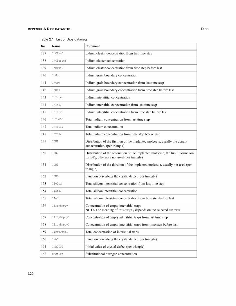
DIOSAPPENDIX A DIOS DATASETS
137 InClusO Indium cluster concentration from last time step
138 InCluster Indium cluster concentration
139 InClusU Indium cluster concentration from time step before last
140 InGbc Indium grain boundary concentration
141 InGbO Indium grain boundary concentration from last time step
142 InGbU Indium grain boundary concentration from time step before last
143 InInter Indium interstitial concentration
144 InIntO Indium interstitial concentration from last time step
145 InIntU Indium interstitial concentration from time step before last
146 InToOld Total indium concentration from last time step
147 InTotal Total indium concentration
148 InToUr Total indium concentration from time step before last
149 ION1 Distribution of the first ion of the implanted molecule, usually the dopant concentration, (per triangle)
150 ION2 Distribution of the second ion of the implanted molecule, the first fluorine ion for BF2, otherwise not used (per triangle)
151 ION3 Distribution of the third ion of the implanted molecule, usually not used (per triangle)
152 IONS Function describing the crystal defect (per triangle)
153 IToOld Total silicon interstitial concentration from last time step
154 ITotal Total silicon interstitial concentration
155 IToUr Total silicon interstitial concentration from time step before last
156 ITrapEmpty Concentration of empty interstitial trapsNOTE The meaning of ITrapEmpty depends on the selected TRAPMOD.
157 ITrapEmptyO Concentration of empty interstitial traps from last time step
158 ITrapEmptyU Concentration of empty interstitial traps from time step before last
159 ITrapTotal Total concentration of interstitial traps
160 IVAC Function describing the crystal defect (per triangle)
161 IVACINI Initial value of crystal defect (per triangle)
162 NActive Substitutional nitrogen concentration
Table 27 List of Dios datasets
No. Name Comment
320
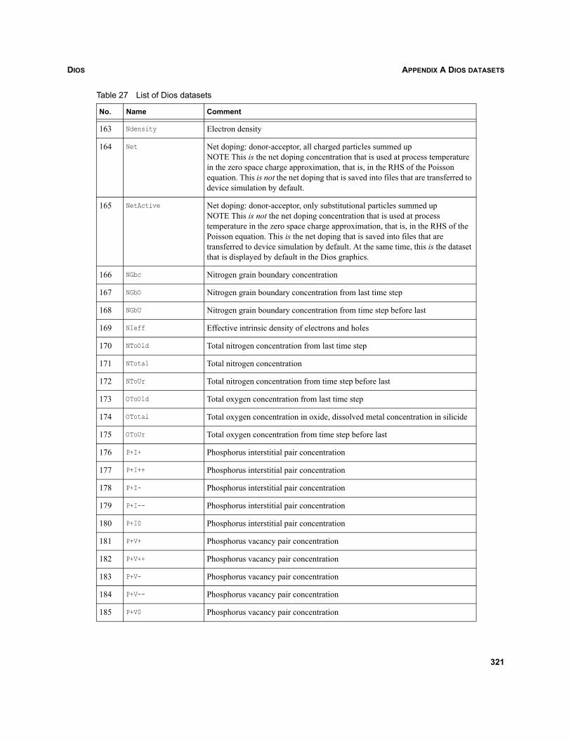
DIOS APPENDIX A DIOS DATASETS
163 Ndensity Electron density
164 Net Net doping: donor-acceptor, all charged particles summed upNOTE This is the net doping concentration that is used at process temperature in the zero space charge approximation, that is, in the RHS of the Poisson equation. This is not the net doping that is saved into files that are transferred to device simulation by default.
165 NetActive Net doping: donor-acceptor, only substitutional particles summed upNOTE This is not the net doping concentration that is used at process temperature in the zero space charge approximation, that is, in the RHS of the Poisson equation. This is the net doping that is saved into files that are transferred to device simulation by default. At the same time, this is the dataset that is displayed by default in the Dios graphics.
166 NGbc Nitrogen grain boundary concentration
167 NGbO Nitrogen grain boundary concentration from last time step
168 NGbU Nitrogen grain boundary concentration from time step before last
169 NIeff Effective intrinsic density of electrons and holes
170 NToOld Total nitrogen concentration from last time step
171 NTotal Total nitrogen concentration
172 NToUr Total nitrogen concentration from time step before last
173 OToOld Total oxygen concentration from last time step
174 OTotal Total oxygen concentration in oxide, dissolved metal concentration in silicide
175 OToUr Total oxygen concentration from time step before last
176 P+I+ Phosphorus interstitial pair concentration
177 P+I++ Phosphorus interstitial pair concentration
178 P+I- Phosphorus interstitial pair concentration
179 P+I-- Phosphorus interstitial pair concentration
180 P+I0 Phosphorus interstitial pair concentration
181 P+V+ Phosphorus vacancy pair concentration
182 P+V++ Phosphorus vacancy pair concentration
183 P+V- Phosphorus vacancy pair concentration
184 P+V-- Phosphorus vacancy pair concentration
185 P+V0 Phosphorus vacancy pair concentration
Table 27 List of Dios datasets
No. Name Comment
321
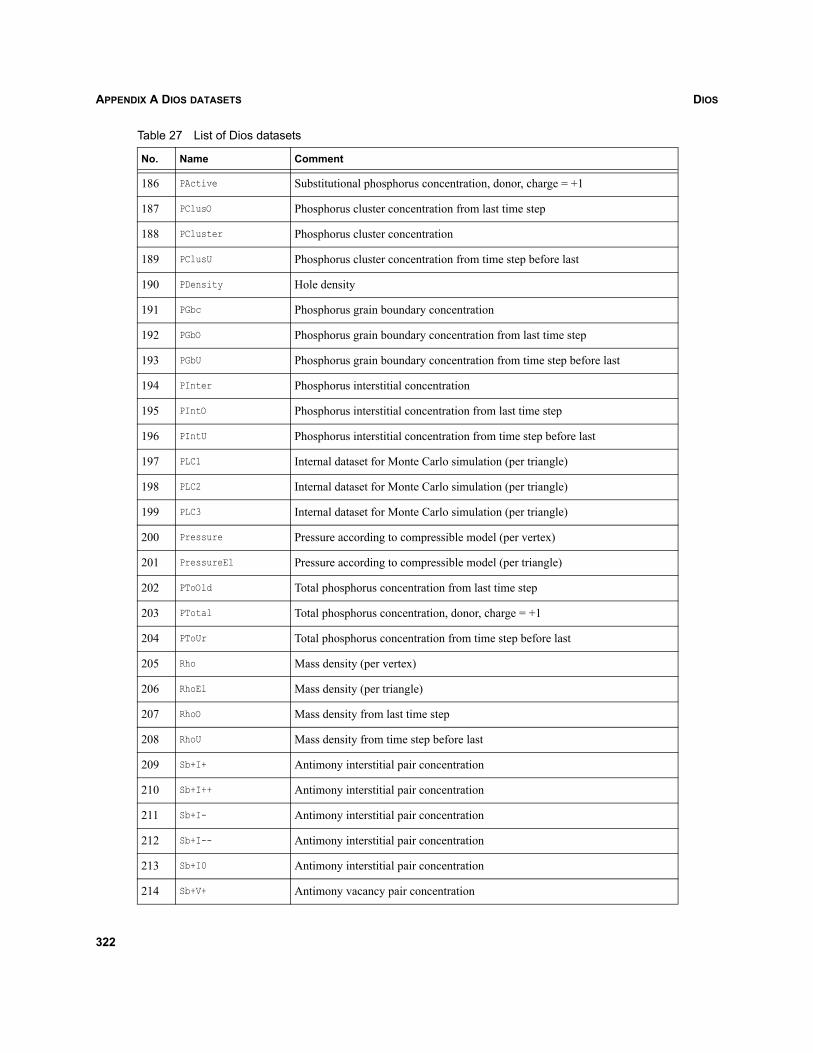
DIOSAPPENDIX A DIOS DATASETS
186 PActive Substitutional phosphorus concentration, donor, charge = +1
187 PClusO Phosphorus cluster concentration from last time step
188 PCluster Phosphorus cluster concentration
189 PClusU Phosphorus cluster concentration from time step before last
190 PDensity Hole density
191 PGbc Phosphorus grain boundary concentration
192 PGbO Phosphorus grain boundary concentration from last time step
193 PGbU Phosphorus grain boundary concentration from time step before last
194 PInter Phosphorus interstitial concentration
195 PIntO Phosphorus interstitial concentration from last time step
196 PIntU Phosphorus interstitial concentration from time step before last
197 PLC1 Internal dataset for Monte Carlo simulation (per triangle)
198 PLC2 Internal dataset for Monte Carlo simulation (per triangle)
199 PLC3 Internal dataset for Monte Carlo simulation (per triangle)
200 Pressure Pressure according to compressible model (per vertex)
201 PressureEl Pressure according to compressible model (per triangle)
202 PToOld Total phosphorus concentration from last time step
203 PTotal Total phosphorus concentration, donor, charge = +1
204 PToUr Total phosphorus concentration from time step before last
205 Rho Mass density (per vertex)
206 RhoEl Mass density (per triangle)
207 RhoO Mass density from last time step
208 RhoU Mass density from time step before last
209 Sb+I+ Antimony interstitial pair concentration
210 Sb+I++ Antimony interstitial pair concentration
211 Sb+I- Antimony interstitial pair concentration
212 Sb+I-- Antimony interstitial pair concentration
213 Sb+I0 Antimony interstitial pair concentration
214 Sb+V+ Antimony vacancy pair concentration
Table 27 List of Dios datasets
No. Name Comment
322
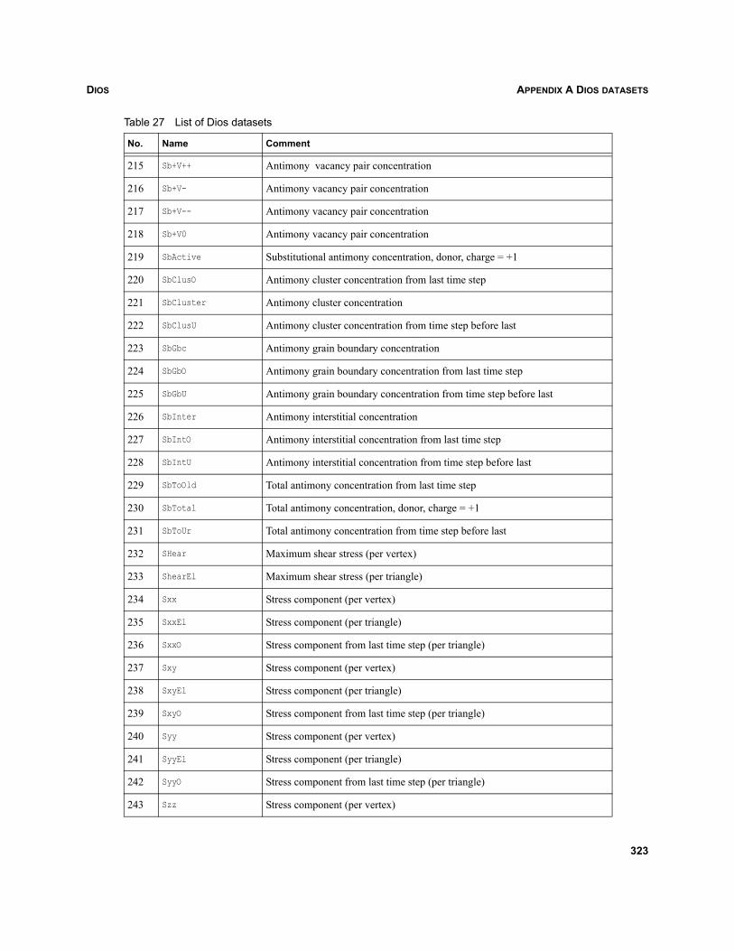
DIOS APPENDIX A DIOS DATASETS
215 Sb+V++ Antimony vacancy pair concentration
216 Sb+V- Antimony vacancy pair concentration
217 Sb+V-- Antimony vacancy pair concentration
218 Sb+V0 Antimony vacancy pair concentration
219 SbActive Substitutional antimony concentration, donor, charge = +1
220 SbClusO Antimony cluster concentration from last time step
221 SbCluster Antimony cluster concentration
222 SbClusU Antimony cluster concentration from time step before last
223 SbGbc Antimony grain boundary concentration
224 SbGbO Antimony grain boundary concentration from last time step
225 SbGbU Antimony grain boundary concentration from time step before last
226 SbInter Antimony interstitial concentration
227 SbIntO Antimony interstitial concentration from last time step
228 SbIntU Antimony interstitial concentration from time step before last
229 SbToOld Total antimony concentration from last time step
230 SbTotal Total antimony concentration, donor, charge = +1
231 SbToUr Total antimony concentration from time step before last
232 SHear Maximum shear stress (per vertex)
233 ShearEl Maximum shear stress (per triangle)
234 Sxx Stress component (per vertex)
235 SxxEl Stress component (per triangle)
236 SxxO Stress component from last time step (per triangle)
237 Sxy Stress component (per vertex)
238 SxyEl Stress component (per triangle)
239 SxyO Stress component from last time step (per triangle)
240 Syy Stress component (per vertex)
241 SyyEl Stress component (per triangle)
242 SyyO Stress component from last time step (per triangle)
243 Szz Stress component (per vertex)
Table 27 List of Dios datasets
No. Name Comment
323
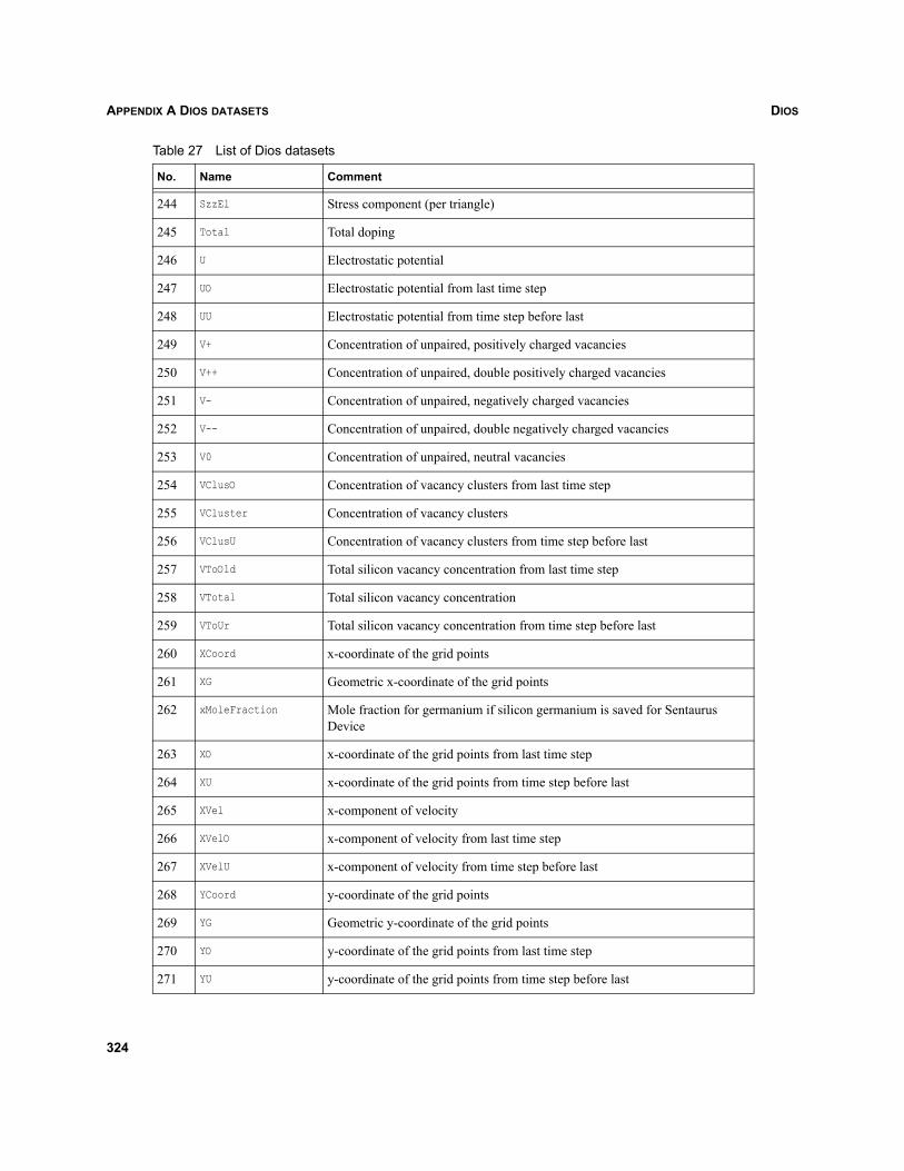
DIOSAPPENDIX A DIOS DATASETS
244 SzzEl Stress component (per triangle)
245 Total Total doping
246 U Electrostatic potential
247 UO Electrostatic potential from last time step
248 UU Electrostatic potential from time step before last
249 V+ Concentration of unpaired, positively charged vacancies
250 V++ Concentration of unpaired, double positively charged vacancies
251 V- Concentration of unpaired, negatively charged vacancies
252 V-- Concentration of unpaired, double negatively charged vacancies
253 V0 Concentration of unpaired, neutral vacancies
254 VClusO Concentration of vacancy clusters from last time step
255 VCluster Concentration of vacancy clusters
256 VClusU Concentration of vacancy clusters from time step before last
257 VToOld Total silicon vacancy concentration from last time step
258 VTotal Total silicon vacancy concentration
259 VToUr Total silicon vacancy concentration from time step before last
260 XCoord x-coordinate of the grid points
261 XG Geometric x-coordinate of the grid points
262 xMoleFraction Mole fraction for germanium if silicon germanium is saved for Sentaurus Device
263 XO x-coordinate of the grid points from last time step
264 XU x-coordinate of the grid points from time step before last
265 XVel x-component of velocity
266 XVelO x-component of velocity from last time step
267 XVelU x-component of velocity from time step before last
268 YCoord y-coordinate of the grid points
269 YG Geometric y-coordinate of the grid points
270 YO y-coordinate of the grid points from last time step
271 YU y-coordinate of the grid points from time step before last
Table 27 List of Dios datasets
No. Name Comment
324

DIOS APPENDIX A DIOS DATASETS
272 YVel y-component of velocity
273 YVelO y-component of velocity from last time step
274 YVelU y-component of velocity from time step before last
Table 27 List of Dios datasets
No. Name Comment
325

DIOSAPPENDIX A DIOS DATASETS
326
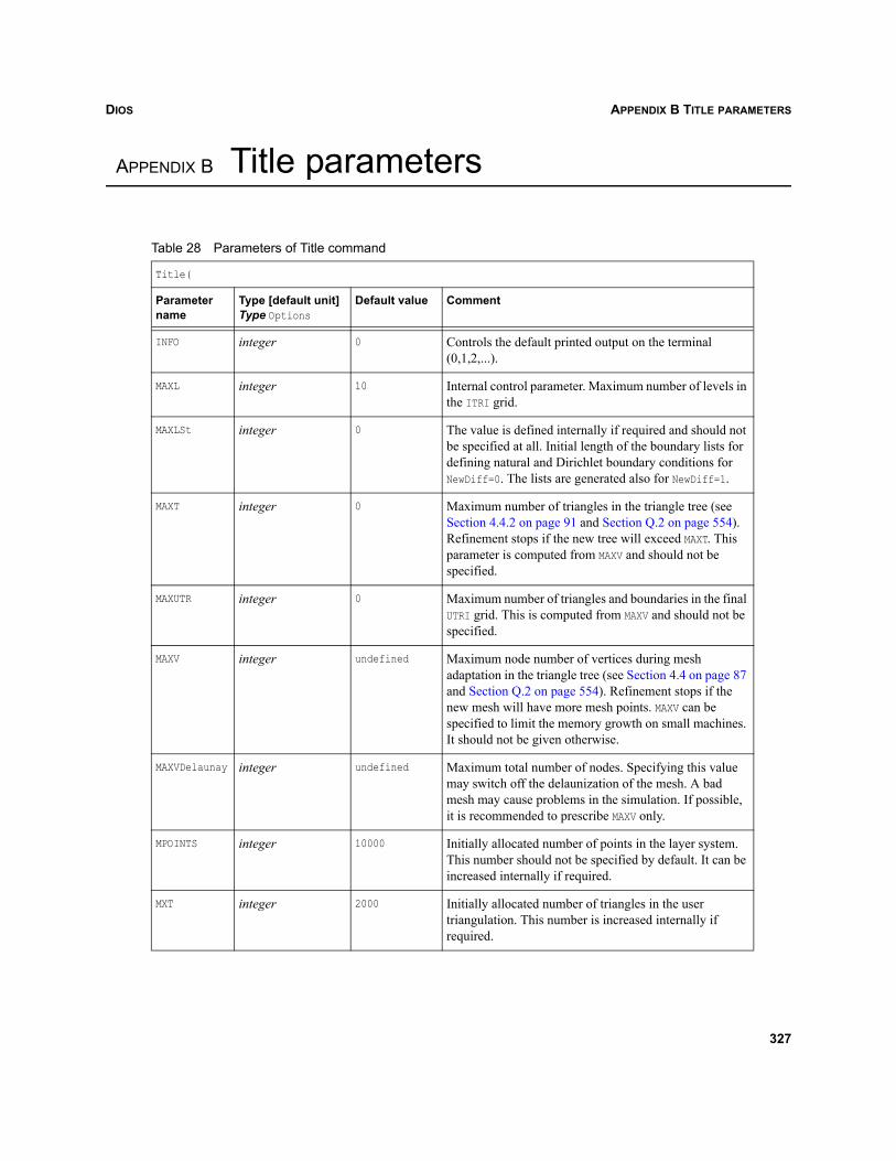
DIOS APPENDIX B TITLE PARAMETERS
Dios
APPENDIX B Title parameters
Table 28 Parameters of Title command
Title(
Parameter name
Type [default unit]Type Options
Default value Comment
INFO integer 0 Controls the default printed output on the terminal (0,1,2,...).
MAXL integer 10 Internal control parameter. Maximum number of levels in the ITRI grid.
MAXLSt integer 0 The value is defined internally if required and should not be specified at all. Initial length of the boundary lists for defining natural and Dirichlet boundary conditions for NewDiff=0. The lists are generated also for NewDiff=1.
MAXT integer 0 Maximum number of triangles in the triangle tree (see Section 4.4.2 on page 91 and Section Q.2 on page 554). Refinement stops if the new tree will exceed MAXT. This parameter is computed from MAXV and should not be specified.
MAXUTR integer 0 Maximum number of triangles and boundaries in the final UTRI grid. This is computed from MAXV and should not be specified.
MAXV integer undefined Maximum node number of vertices during mesh adaptation in the triangle tree (see Section 4.4 on page 87 and Section Q.2 on page 554). Refinement stops if the new mesh will have more mesh points. MAXV can be specified to limit the memory growth on small machines. It should not be given otherwise.
MAXVDelaunay integer undefined Maximum total number of nodes. Specifying this value may switch off the delaunization of the mesh. A bad mesh may cause problems in the simulation. If possible, it is recommended to prescribe MAXV only.
MPOINTS integer 10000 Initially allocated number of points in the layer system. This number should not be specified by default. It can be increased internally if required.
MXT integer 2000 Initially allocated number of triangles in the user triangulation. This number is increased internally if required.
327
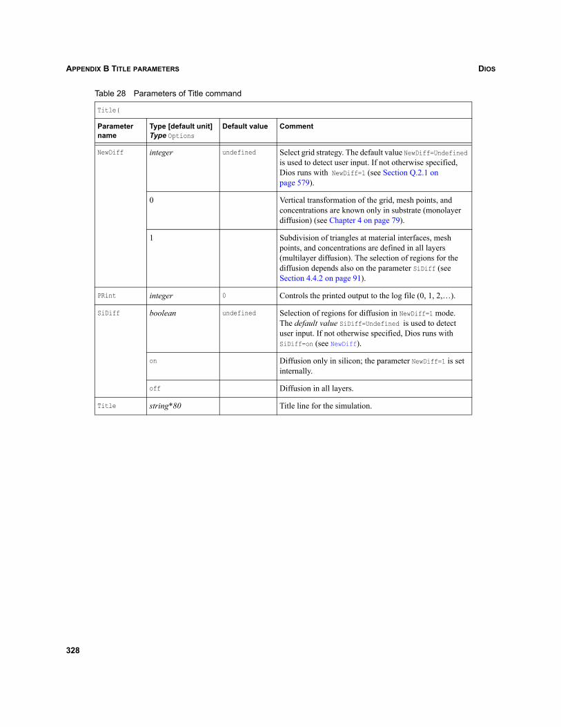
DIOSAPPENDIX B TITLE PARAMETERS
NewDiff integer undefined Select grid strategy. The default value NewDiff=Undefined is used to detect user input. If not otherwise specified, Dios runs with NewDiff=1 (see Section Q.2.1 on page 579).
0 Vertical transformation of the grid, mesh points, and concentrations are known only in substrate (monolayer diffusion) (see Chapter 4 on page 79).
1 Subdivision of triangles at material interfaces, mesh points, and concentrations are defined in all layers (multilayer diffusion). The selection of regions for the diffusion depends also on the parameter SiDiff (see Section 4.4.2 on page 91).
PRint integer 0 Controls the printed output to the log file (0, 1, 2,…).
SiDiff boolean undefined Selection of regions for diffusion in NewDiff=1 mode.The default value SiDiff=Undefined is used to detect user input. If not otherwise specified, Dios runs with SiDiff=on (see NewDiff).
on Diffusion only in silicon; the parameter NewDiff=1 is set internally.
off Diffusion in all layers.
Title string*80 Title line for the simulation.
Table 28 Parameters of Title command
Title(
Parameter name
Type [default unit]Type Options
Default value Comment
328
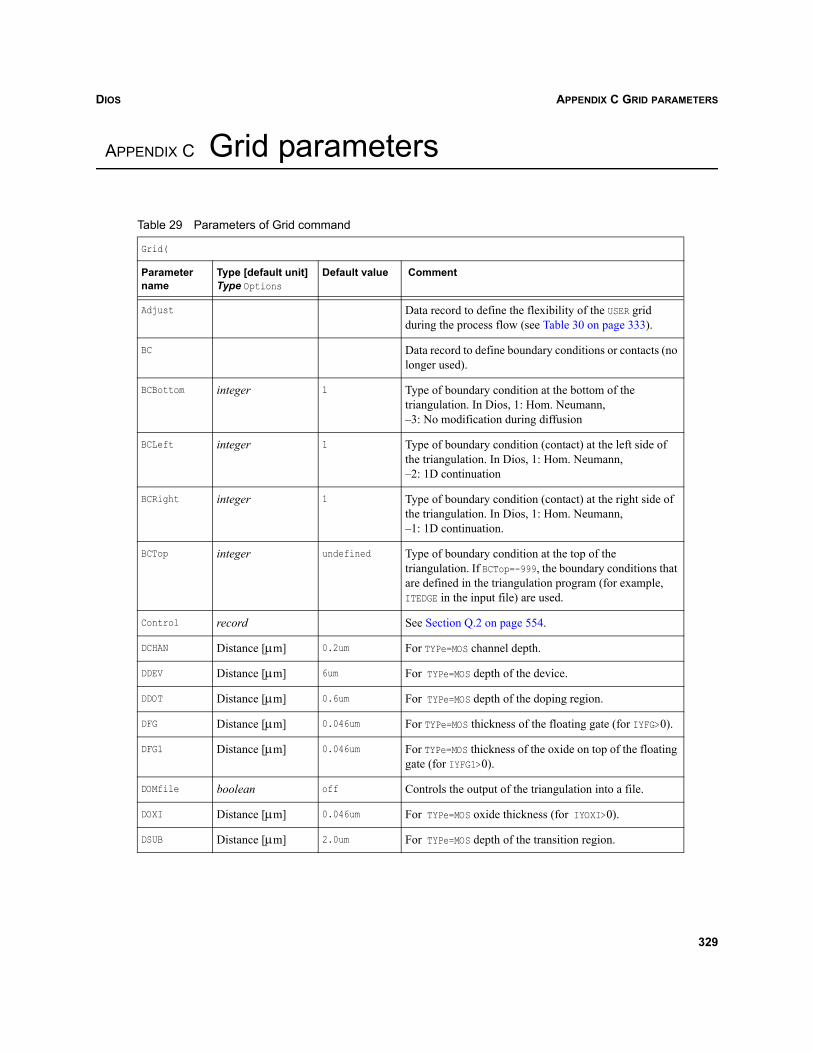
DIOS APPENDIX C GRID PARAMETERS
Dios
APPENDIX C Grid parameters
Table 29 Parameters of Grid command
Grid(
Parameter name
Type [default unit]Type Options
Default value Comment
Adjust Data record to define the flexibility of the USER grid during the process flow (see Table 30 on page 333).
BC Data record to define boundary conditions or contacts (no longer used).
BCBottom integer 1 Type of boundary condition at the bottom of the triangulation. In Dios, 1: Hom. Neumann, –3: No modification during diffusion
BCLeft integer 1 Type of boundary condition (contact) at the left side of the triangulation. In Dios, 1: Hom. Neumann, –2: 1D continuation
BCRight integer 1 Type of boundary condition (contact) at the right side of the triangulation. In Dios, 1: Hom. Neumann, –1: 1D continuation.
BCTop integer undefined Type of boundary condition at the top of the triangulation. If BCTop=-999, the boundary conditions that are defined in the triangulation program (for example, ITEDGE in the input file) are used.
Control record See Section Q.2 on page 554.
DCHAN Distance [μm] 0.2um For TYPe=MOS channel depth.
DDEV Distance [μm] 6um For TYPe=MOS depth of the device.
DDOT Distance [μm] 0.6um For TYPe=MOS depth of the doping region.
DFG Distance [μm] 0.046um For TYPe=MOS thickness of the floating gate (for IYFG>0).
DFG1 Distance [μm] 0.046um For TYPe=MOS thickness of the oxide on top of the floating gate (for IYFG1>0).
DOMfile boolean off Controls the output of the triangulation into a file.
DOXI Distance [μm] 0.046um For TYPe=MOS oxide thickness (for IYOXI>0).
DSUB Distance [μm] 2.0um For TYPe=MOS depth of the transition region.
329
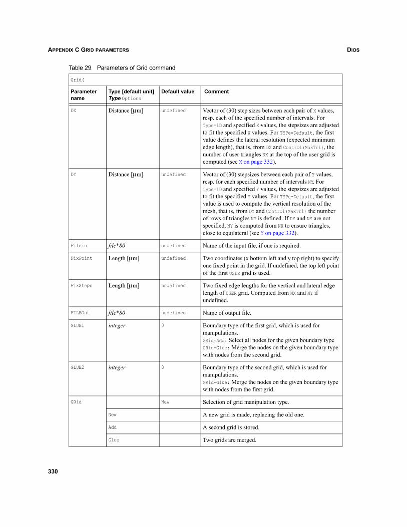
DIOSAPPENDIX C GRID PARAMETERS
DX Distance [μm] undefined Vector of (30) step sizes between each pair of X values, resp. each of the specified number of intervals. For Type=1D and specified X values, the stepsizes are adjusted to fit the specified X values. For TYPe=Default, the first value defines the lateral resolution (expected minimum edge length), that is, from DX and Control(MaxTrl), the number of user triangles NX at the top of the user grid is computed (see X on page 332).
DY Distance [μm] undefined Vector of (30) stepsizes between each pair of Y values, resp. for each specified number of intervals NY. For Type=1D and specified Y values, the stepsizes are adjusted to fit the specified Y values. For TYPe=Default, the first value is used to compute the vertical resolution of the mesh, that is, from DY and Control(MaxTrl) the number of rows of triangles NY is defined. If DY and NY are not specified, NY is computed from NX to ensure triangles, close to equilateral (see Y on page 332).
Filein file*80 undefined Name of the input file, if one is required.
FixPoint Length [μm] undefined Two coordinates (x bottom left and y top right) to specify one fixed point in the grid. If undefined, the top left point of the first USER grid is used.
FixSteps Length [μm] undefined Two fixed edge lengths for the vertical and lateral edge length of USER grid. Computed from NX and NY if undefined.
FILEOut file*80 undefined Name of output file.
GLUE1 integer 0 Boundary type of the first grid, which is used for manipulations.GRid=Add: Select all nodes for the given boundary type GRid=Glue: Merge the nodes on the given boundary type with nodes from the second grid.
GLUE2 integer 0 Boundary type of the second grid, which is used for manipulations.GRid=Glue: Merge the nodes on the given boundary type with nodes from the first grid.
GRid New Selection of grid manipulation type.
New A new grid is made, replacing the old one.
Add A second grid is stored.
Glue Two grids are merged.
Table 29 Parameters of Grid command
Grid(
Parameter name
Type [default unit]Type Options
Default value Comment
330
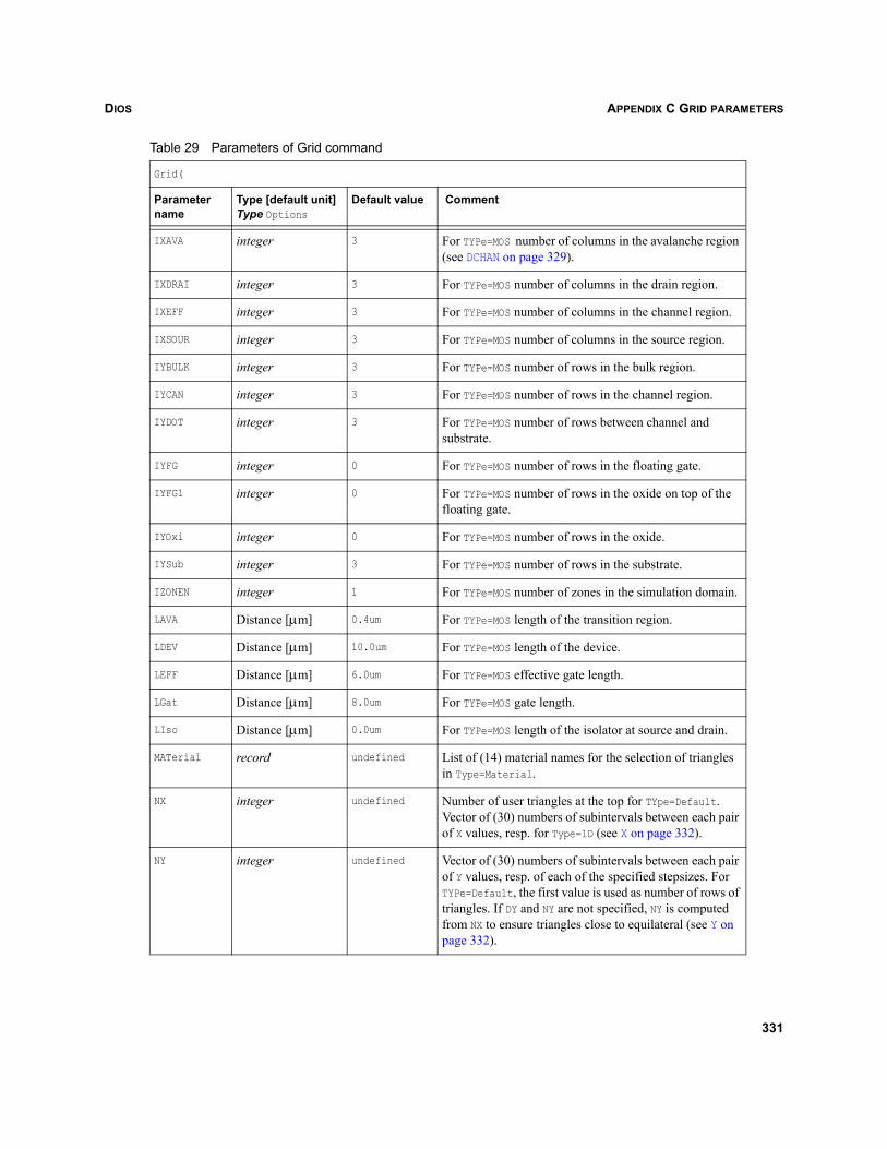
DIOS APPENDIX C GRID PARAMETERS
IXAVA integer 3 For TYPe=MOS number of columns in the avalanche region (see DCHAN on page 329).
IXDRAI integer 3 For TYPe=MOS number of columns in the drain region.
IXEFF integer 3 For TYPe=MOS number of columns in the channel region.
IXSOUR integer 3 For TYPe=MOS number of columns in the source region.
IYBULK integer 3 For TYPe=MOS number of rows in the bulk region.
IYCAN integer 3 For TYPe=MOS number of rows in the channel region.
IYDOT integer 3 For TYPe=MOS number of rows between channel and substrate.
IYFG integer 0 For TYPe=MOS number of rows in the floating gate.
IYFG1 integer 0 For TYPe=MOS number of rows in the oxide on top of the floating gate.
IYOxi integer 0 For TYPe=MOS number of rows in the oxide.
IYSub integer 3 For TYPe=MOS number of rows in the substrate.
IZONEN integer 1 For TYPe=MOS number of zones in the simulation domain.
LAVA Distance [μm] 0.4um For TYPe=MOS length of the transition region.
LDEV Distance [μm] 10.0um For TYPe=MOS length of the device.
LEFF Distance [μm] 6.0um For TYPe=MOS effective gate length.
LGat Distance [μm] 8.0um For TYPe=MOS gate length.
LIso Distance [μm] 0.0um For TYPe=MOS length of the isolator at source and drain.
MATerial record undefined List of (14) material names for the selection of triangles in Type=Material.
NX integer undefined Number of user triangles at the top for TYpe=Default. Vector of (30) numbers of subintervals between each pair of X values, resp. for Type=1D (see X on page 332).
NY integer undefined Vector of (30) numbers of subintervals between each pair of Y values, resp. of each of the specified stepsizes. For TYPe=Default, the first value is used as number of rows of triangles. If DY and NY are not specified, NY is computed from NX to ensure triangles close to equilateral (see Y on page 332).
Table 29 Parameters of Grid command
Grid(
Parameter name
Type [default unit]Type Options
Default value Comment
331
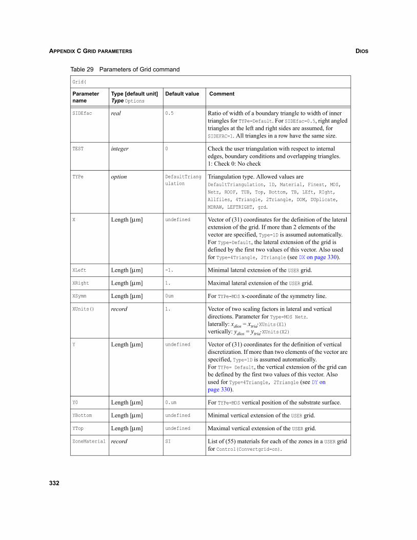
DIOSAPPENDIX C GRID PARAMETERS
SIDEfac real 0.5 Ratio of width of a boundary triangle to width of inner triangles for TYPe=Default. For SIDEfac=0.5, right angled triangles at the left and right sides are assumed, for SIDEFAC=1. All triangles in a row have the same size.
TEST integer 0 Check the user triangulation with respect to internal edges, boundary conditions and overlapping triangles. 1: Check 0: No check
TYPe option DefaultTriangulation
Triangulation type. Allowed values are DefaultTriangulation, 1D, Material, Finest, MOS, Netz, ROOF, TUB, Top, Bottom, TB, LEft, RIght, Allfiles, 4Triangle, 2Triangle, DOM, DUplicate, MDRAW, LEFTRIGHT, grd.
X Length [μm] undefined Vector of (31) coordinates for the definition of the lateral extension of the grid. If more than 2 elements of the vector are specified, Type=1D is assumed automatically. For Type=Default, the lateral extension of the grid is defined by the first two values of this vector. Also used for Type=4Triangle, 2Triangle (see DX on page 330).
XLeft Length [μm] -1. Minimal lateral extension of the USER grid.
XRight Length [μm] 1. Maximal lateral extension of the USER grid.
XSymm Length [μm] 0um For TYPe=MOS x-coordinate of the symmetry line.
XUnits() record 1. Vector of two scaling factors in lateral and vertical directions. Parameter for Type=MOS Netz.laterally: xdios = xtria⋅XUnits(X1)vertically: ydios = ytria⋅XUnits(X2)
Y Length [μm] undefined Vector of (31) coordinates for the definition of vertical discretization. If more than two elements of the vector are specified, Type=1D is assumed automatically. For TYPe= Default, the vertical extension of the grid can be defined by the first two values of this vector. Also used for Type=4Triangle, 2Triangle (see DY on page 330).
Y0 Length [μm] 0.um For TYPe=MOS vertical position of the substrate surface.
YBottom Length [μm] undefined Minimal vertical extension of the USER grid.
YTop Length [μm] undefined Maximal vertical extension of the USER grid.
ZoneMaterial record SI List of (55) materials for each of the zones in a USER grid for Control(Convertgrid=on).
Table 29 Parameters of Grid command
Grid(
Parameter name
Type [default unit]Type Options
Default value Comment
332
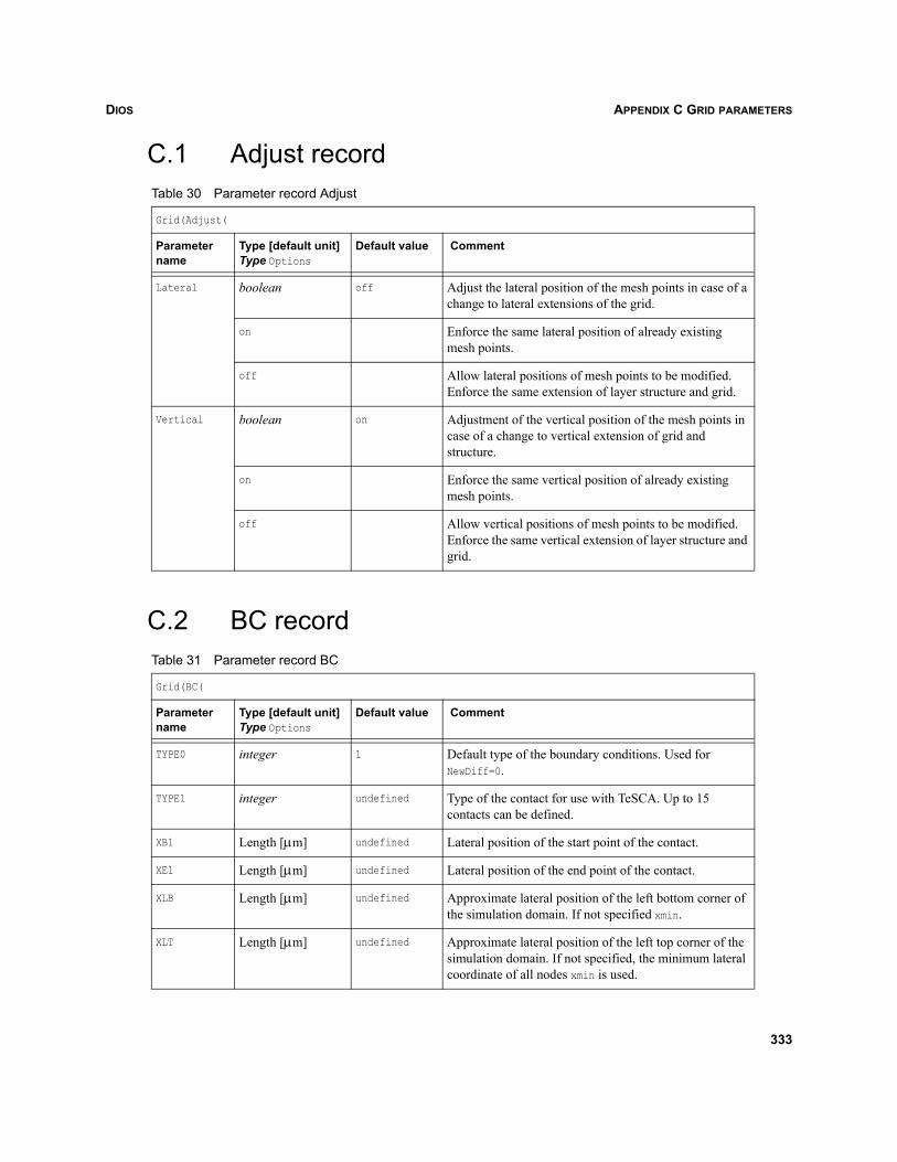
DIOS APPENDIX C GRID PARAMETERS
C.1 Adjust record
C.2 BC record
Table 30 Parameter record Adjust
Grid(Adjust(
Parameter name
Type [default unit]Type Options
Default value Comment
Lateral boolean off Adjust the lateral position of the mesh points in case of a change to lateral extensions of the grid.
on Enforce the same lateral position of already existing mesh points.
off Allow lateral positions of mesh points to be modified. Enforce the same extension of layer structure and grid.
Vertical boolean on Adjustment of the vertical position of the mesh points in case of a change to vertical extension of grid and structure.
on Enforce the same vertical position of already existing mesh points.
off Allow vertical positions of mesh points to be modified. Enforce the same vertical extension of layer structure and grid.
Table 31 Parameter record BC
Grid(BC(
Parameter name
Type [default unit]Type Options
Default value Comment
TYPE0 integer 1 Default type of the boundary conditions. Used for NewDiff=0.
TYPE1 integer undefined Type of the contact for use with TeSCA. Up to 15 contacts can be defined.
XB1 Length [μm] undefined Lateral position of the start point of the contact.
XE1 Length [μm] undefined Lateral position of the end point of the contact.
XLB Length [μm] undefined Approximate lateral position of the left bottom corner of the simulation domain. If not specified xmin.
XLT Length [μm] undefined Approximate lateral position of the left top corner of the simulation domain. If not specified, the minimum lateral coordinate of all nodes xmin is used.
333
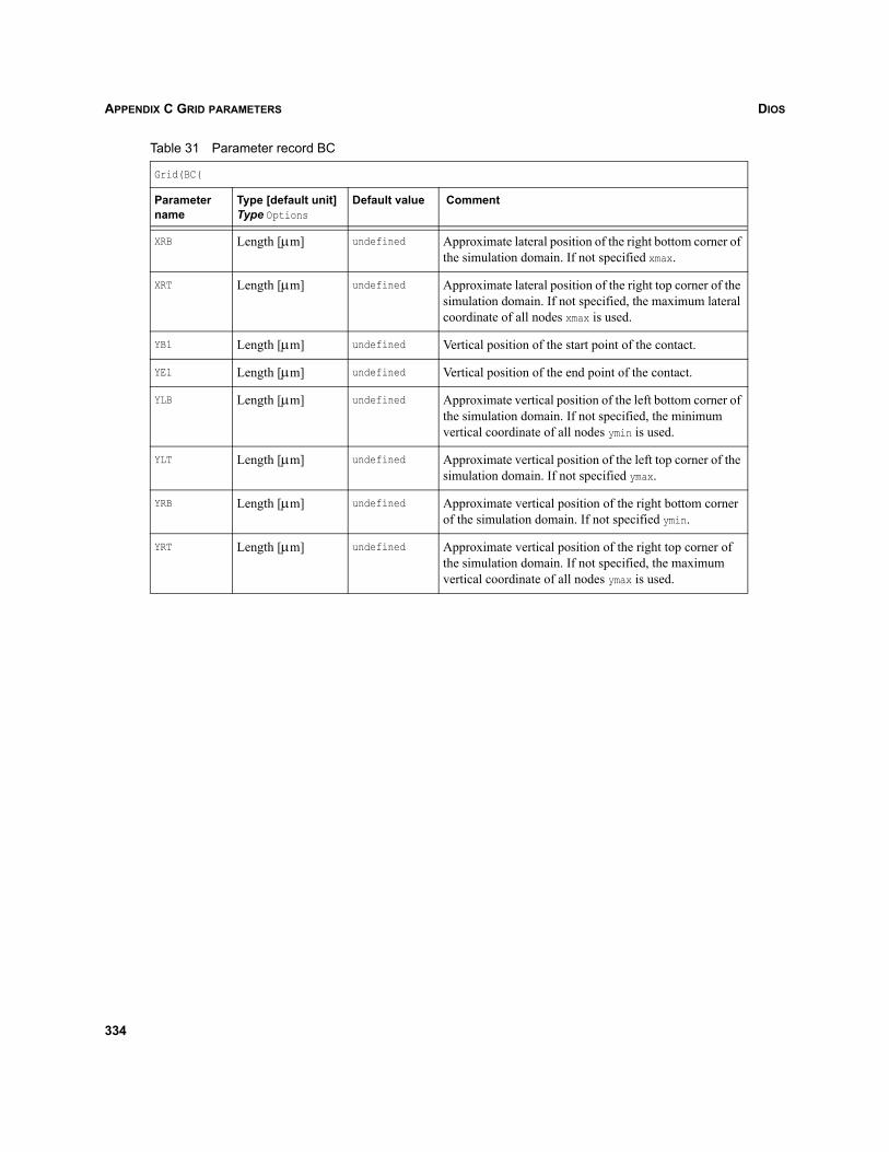
DIOSAPPENDIX C GRID PARAMETERS
XRB Length [μm] undefined Approximate lateral position of the right bottom corner of the simulation domain. If not specified xmax.
XRT Length [μm] undefined Approximate lateral position of the right top corner of the simulation domain. If not specified, the maximum lateral coordinate of all nodes xmax is used.
YB1 Length [μm] undefined Vertical position of the start point of the contact.
YE1 Length [μm] undefined Vertical position of the end point of the contact.
YLB Length [μm] undefined Approximate vertical position of the left bottom corner of the simulation domain. If not specified, the minimum vertical coordinate of all nodes ymin is used.
YLT Length [μm] undefined Approximate vertical position of the left top corner of the simulation domain. If not specified ymax.
YRB Length [μm] undefined Approximate vertical position of the right bottom corner of the simulation domain. If not specified ymin.
YRT Length [μm] undefined Approximate vertical position of the right top corner of the simulation domain. If not specified, the maximum vertical coordinate of all nodes ymax is used.
Table 31 Parameter record BC
Grid(BC(
Parameter name
Type [default unit]Type Options
Default value Comment
334
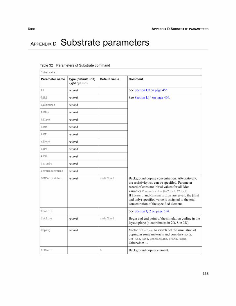
DIOS APPENDIX D SUBSTRATE PARAMETERS
Dios
APPENDIX D Substrate parameters
Table 32 Parameters of Substrate command
Substrate(
Parameter name Type [default unit]Type Options
Default value Comment
Al record See Section I.9 on page 455.
AlAl record See Section I.14 on page 466.
AlCeramic record
AlGas record
AlIsoX record
AlMe record
AlMS record
AlOxyN record
AlPo record
AlSG record
Ceramic record
CeramicCeramic record
CONCentration record undefined Background doping concentration. Alternatively, the resistivity RHO can be specified. Parameter record of constant initial values for all Dios variables Concentration(AsTotal BTotal).If Element and Concentration are given, the (first and only) specified value is assigned to the total concentration of the specified element.
Control See Section Q.2 on page 554.
Cutline record undefined Begin and end point of the simulation cutline in the layout plane (4 coordinates in 2D, 8 in 3D).
Doping record Vector of boolean to switch off the simulation of doping in some materials and boundary sorts.Off: Gas, Rand, LRand, ORand, URand, RRand Otherwise: On
ELEMent B Background doping element.
335
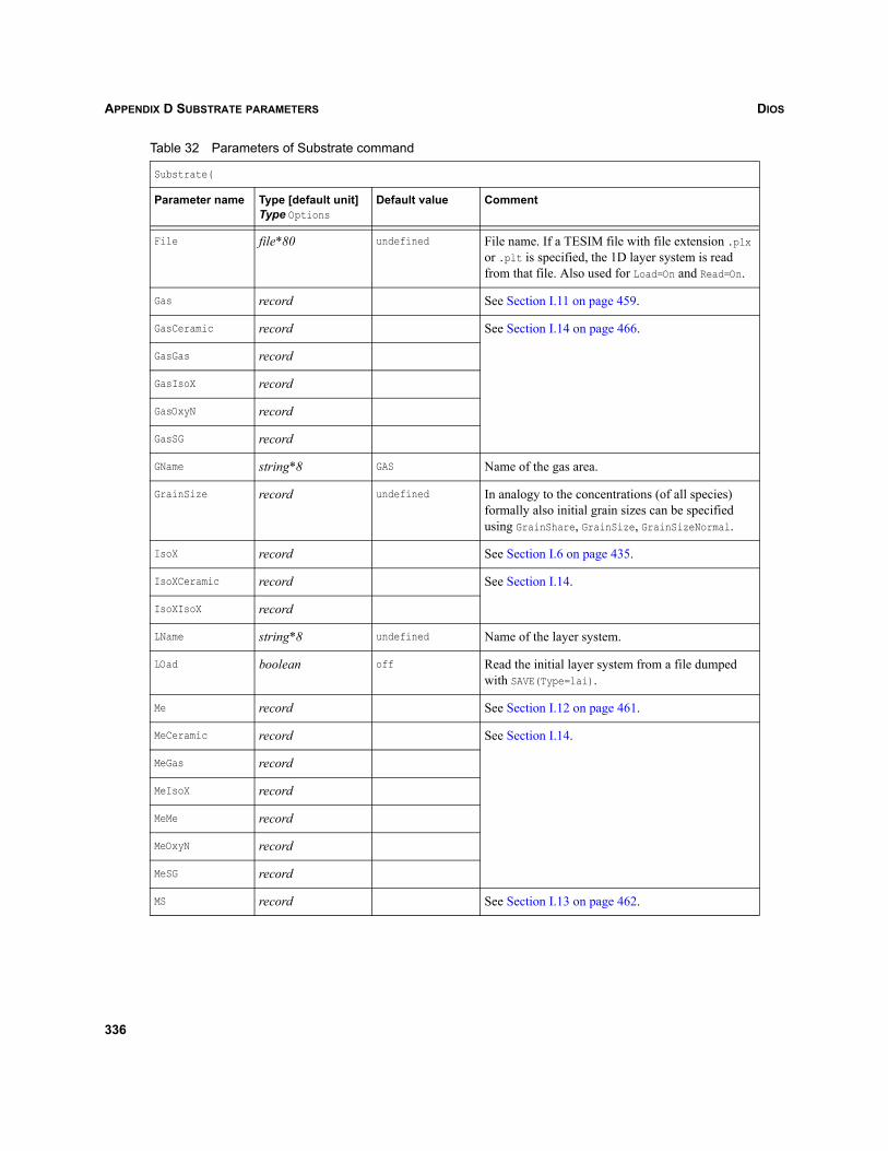
DIOSAPPENDIX D SUBSTRATE PARAMETERS
File file*80 undefined File name. If a TESIM file with file extension .plx or .plt is specified, the 1D layer system is read from that file. Also used for Load=On and Read=On.
Gas record See Section I.11 on page 459.
GasCeramic record See Section I.14 on page 466.
GasGas record
GasIsoX record
GasOxyN record
GasSG record
GName string*8 GAS Name of the gas area.
GrainSize record undefined In analogy to the concentrations (of all species) formally also initial grain sizes can be specified using GrainShare, GrainSize, GrainSizeNormal.
IsoX record See Section I.6 on page 435.
IsoXCeramic record See Section I.14.
IsoXIsoX record
LName string*8 undefined Name of the layer system.
LOad boolean off Read the initial layer system from a file dumped with SAVE(Type=lai).
Me record See Section I.12 on page 461.
MeCeramic record See Section I.14.
MeGas record
MeIsoX record
MeMe record
MeOxyN record
MeSG record
MS record See Section I.13 on page 462.
Table 32 Parameters of Substrate command
Substrate(
Parameter name Type [default unit]Type Options
Default value Comment
336
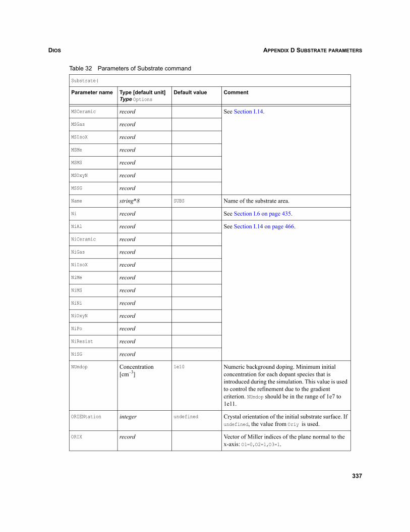
DIOS APPENDIX D SUBSTRATE PARAMETERS
MSCeramic record See Section I.14.
MSGas record
MSIsoX record
MSMe record
MSMS record
MSOxyN record
MSSG record
Name string*8 SUBS Name of the substrate area.
Ni record See Section I.6 on page 435.
NiAl record See Section I.14 on page 466.
NiCeramic record
NiGas record
NiIsoX record
NiMe record
NiMS record
NiNi record
NiOxyN record
NiPo record
NiResist record
NiSG record
NUmdop Concentration [cm–3]
1e10 Numeric background doping. Minimum initial concentration for each dopant species that is introduced during the simulation. This value is used to control the refinement due to the gradient criterion. NUmdop should be in the range of 1e7 to 1e11.
ORIENtation integer undefined Crystal orientation of the initial substrate surface. If undefined, the value from Oriy is used.
ORIX record Vector of Miller indices of the plane normal to the x-axis: O1=0,O2=1,O3=1.
Table 32 Parameters of Substrate command
Substrate(
Parameter name Type [default unit]Type Options
Default value Comment
337
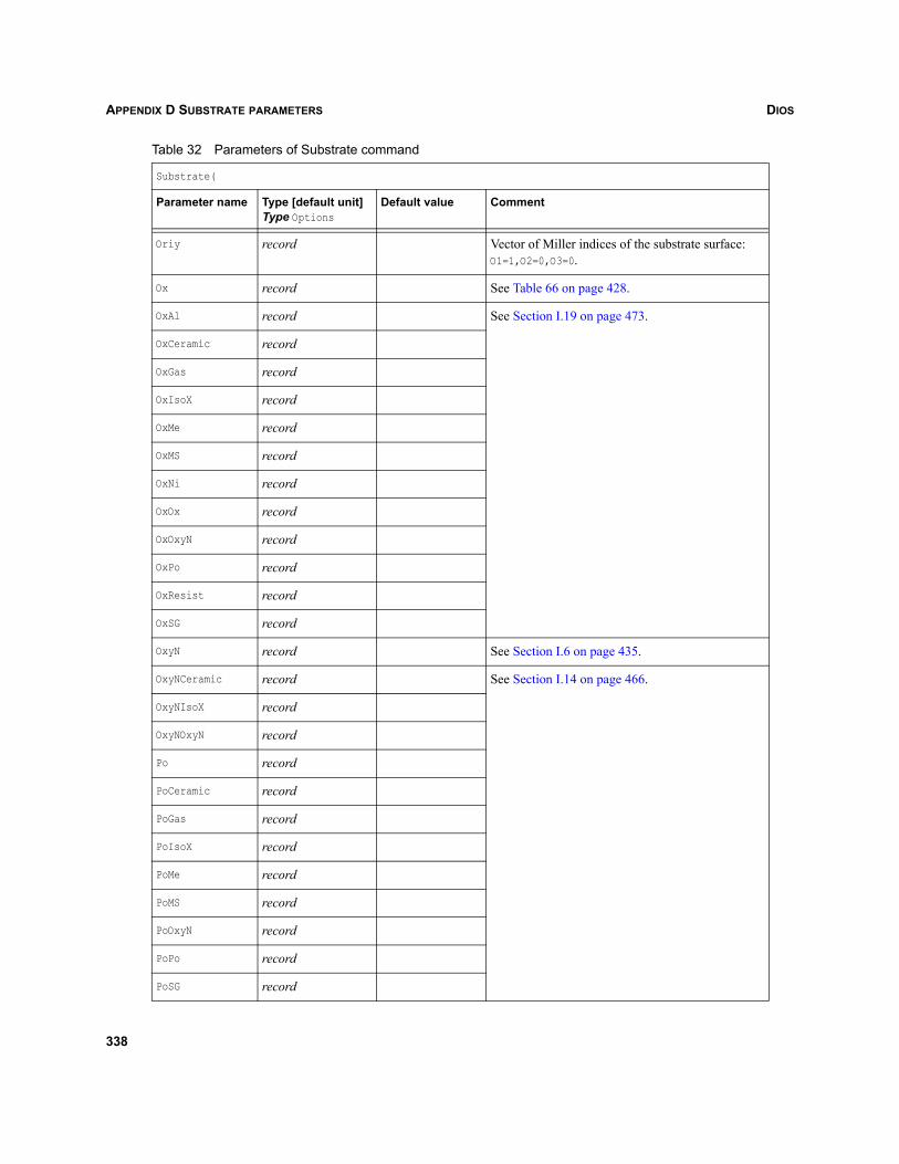
DIOSAPPENDIX D SUBSTRATE PARAMETERS
Oriy record Vector of Miller indices of the substrate surface: O1=1,O2=0,O3=0.
Ox record See Table 66 on page 428.
OxAl record See Section I.19 on page 473.
OxCeramic record
OxGas record
OxIsoX record
OxMe record
OxMS record
OxNi record
OxOx record
OxOxyN record
OxPo record
OxResist record
OxSG record
OxyN record See Section I.6 on page 435.
OxyNCeramic record See Section I.14 on page 466.
OxyNIsoX record
OxyNOxyN record
Po record
PoCeramic record
PoGas record
PoIsoX record
PoMe record
PoMS record
PoOxyN record
PoPo record
PoSG record
Table 32 Parameters of Substrate command
Substrate(
Parameter name Type [default unit]Type Options
Default value Comment
338
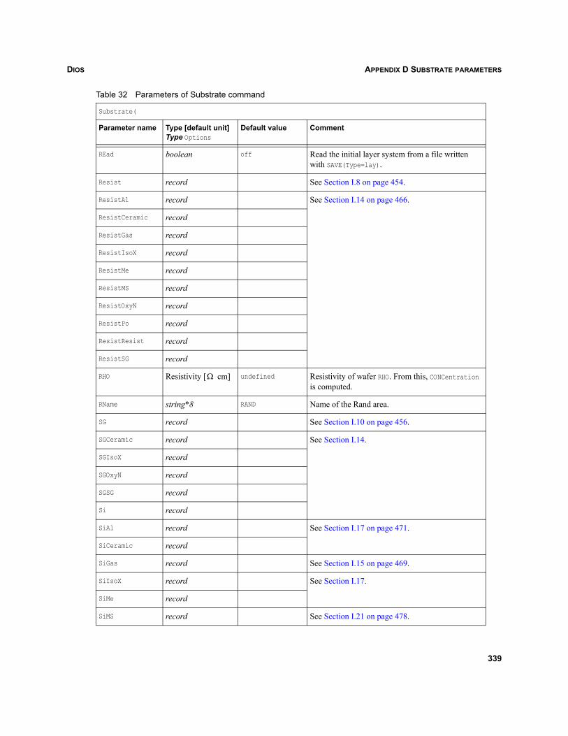
DIOS APPENDIX D SUBSTRATE PARAMETERS
REad boolean off Read the initial layer system from a file written with SAVE(Type=lay).
Resist record See Section I.8 on page 454.
ResistAl record See Section I.14 on page 466.
ResistCeramic record
ResistGas record
ResistIsoX record
ResistMe record
ResistMS record
ResistOxyN record
ResistPo record
ResistResist record
ResistSG record
RHO Resistivity [ cm] undefined Resistivity of wafer RHO. From this, CONCentration is computed.
RName string*8 RAND Name of the Rand area.
SG record See Section I.10 on page 456.
SGCeramic record See Section I.14.
SGIsoX record
SGOxyN record
SGSG record
Si record
SiAl record See Section I.17 on page 471.
SiCeramic record
SiGas record See Section I.15 on page 469.
SiIsoX record See Section I.17.
SiMe record
SiMS record See Section I.21 on page 478.
Table 32 Parameters of Substrate command
Substrate(
Parameter name Type [default unit]Type Options
Default value Comment
Ω
339
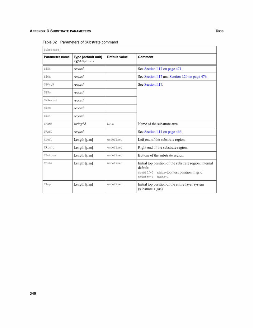
DIOSAPPENDIX D SUBSTRATE PARAMETERS
SiNi record See Section I.17 on page 471.
SiOx record See Section I.17 and Section I.20 on page 476.
SiOxyN record See Section I.17.
SiPo record
SiResist record
SiSG record
SiSi record
SName string*8 SUBS Name of the substrate area.
URAND record See Section I.14 on page 466.
XLeft Length [μm] undefined Left end of the substrate region.
XRight Length [μm] undefined Right end of the substrate region.
YBottom Length [μm] undefined Bottom of the substrate region.
YSubs Length [μm] undefined Initial top position of the substrate region, internal default:NewDiff=0: YSubs=topmost position in gridNewDiff=1: YSubs=0
YTop Length [μm] undefined Initial top position of the entire layer system (substrate + gas).
Table 32 Parameters of Substrate command
Substrate(
Parameter name Type [default unit]Type Options
Default value Comment
340
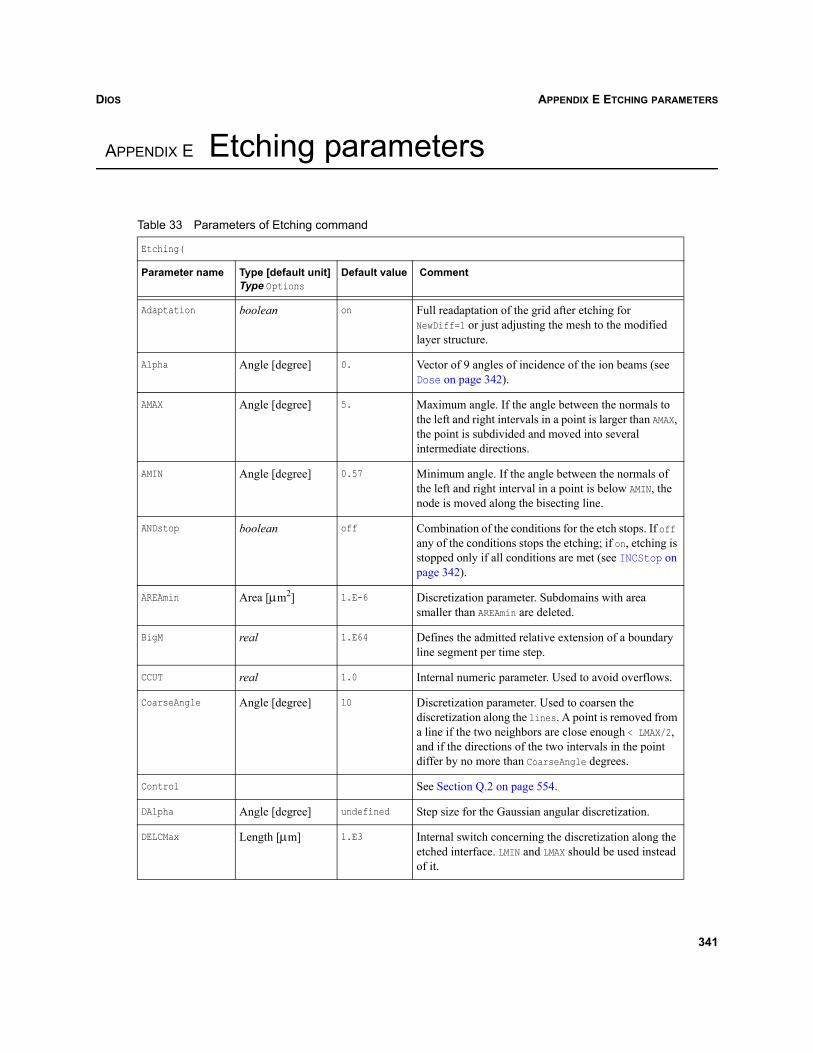
DIOS APPENDIX E ETCHING PARAMETERS
Dios
APPENDIX E Etching parameters
Table 33 Parameters of Etching command
Etching(
Parameter name Type [default unit]Type Options
Default value Comment
Adaptation boolean on Full readaptation of the grid after etching for NewDiff=1 or just adjusting the mesh to the modified layer structure.
Alpha Angle [degree] 0. Vector of 9 angles of incidence of the ion beams (see Dose on page 342).
AMAX Angle [degree] 5. Maximum angle. If the angle between the normals to the left and right intervals in a point is larger than AMAX, the point is subdivided and moved into several intermediate directions.
AMIN Angle [degree] 0.57 Minimum angle. If the angle between the normals of the left and right interval in a point is below AMIN, the node is moved along the bisecting line.
ANDstop boolean off Combination of the conditions for the etch stops. If off any of the conditions stops the etching; if on, etching is stopped only if all conditions are met (see INCStop on page 342).
AREAmin Area [μm2] 1.E-6 Discretization parameter. Subdomains with area smaller than AREAmin are deleted.
BigM real 1.E64 Defines the admitted relative extension of a boundary line segment per time step.
CCUT real 1.0 Internal numeric parameter. Used to avoid overflows.
CoarseAngle Angle [degree] 10 Discretization parameter. Used to coarsen the discretization along the lines. A point is removed from a line if the two neighbors are close enough < LMAX/2, and if the directions of the two intervals in the point differ by no more than CoarseAngle degrees.
Control See Section Q.2 on page 554.
DAlpha Angle [degree] undefined Step size for the Gaussian angular discretization.
DELCMax Length [μm] 1.E3 Internal switch concerning the discretization along the etched interface. LMIN and LMAX should be used instead of it.
341
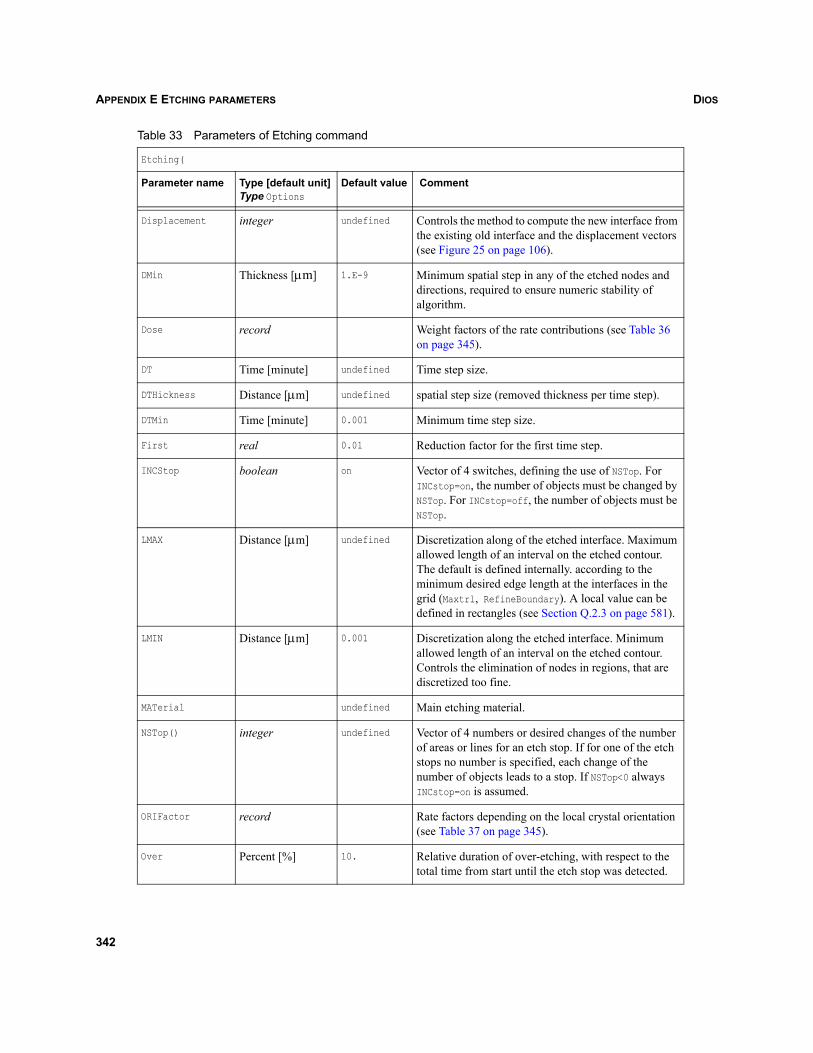
DIOSAPPENDIX E ETCHING PARAMETERS
Displacement integer undefined Controls the method to compute the new interface from the existing old interface and the displacement vectors (see Figure 25 on page 106).
DMin Thickness [μm] 1.E-9 Minimum spatial step in any of the etched nodes and directions, required to ensure numeric stability of algorithm.
Dose record Weight factors of the rate contributions (see Table 36 on page 345).
DT Time [minute] undefined Time step size.
DTHickness Distance [μm] undefined spatial step size (removed thickness per time step).
DTMin Time [minute] 0.001 Minimum time step size.
First real 0.01 Reduction factor for the first time step.
INCStop boolean on Vector of 4 switches, defining the use of NSTop. For INCstop=on, the number of objects must be changed by NSTop. For INCstop=off, the number of objects must be NSTop.
LMAX Distance [μm] undefined Discretization along of the etched interface. Maximum allowed length of an interval on the etched contour. The default is defined internally. according to the minimum desired edge length at the interfaces in the grid (Maxtrl, RefineBoundary). A local value can be defined in rectangles (see Section Q.2.3 on page 581).
LMIN Distance [μm] 0.001 Discretization along the etched interface. Minimum allowed length of an interval on the etched contour. Controls the elimination of nodes in regions, that are discretized too fine.
MATerial undefined Main etching material.
NSTop() integer undefined Vector of 4 numbers or desired changes of the number of areas or lines for an etch stop. If for one of the etch stops no number is specified, each change of the number of objects leads to a stop. If NSTop<0 always INCstop=on is assumed.
ORIFactor record Rate factors depending on the local crystal orientation (see Table 37 on page 345).
Over Percent [%] 10. Relative duration of over-etching, with respect to the total time from start until the etch stop was detected.
Table 33 Parameters of Etching command
Etching(
Parameter name Type [default unit]Type Options
Default value Comment
342
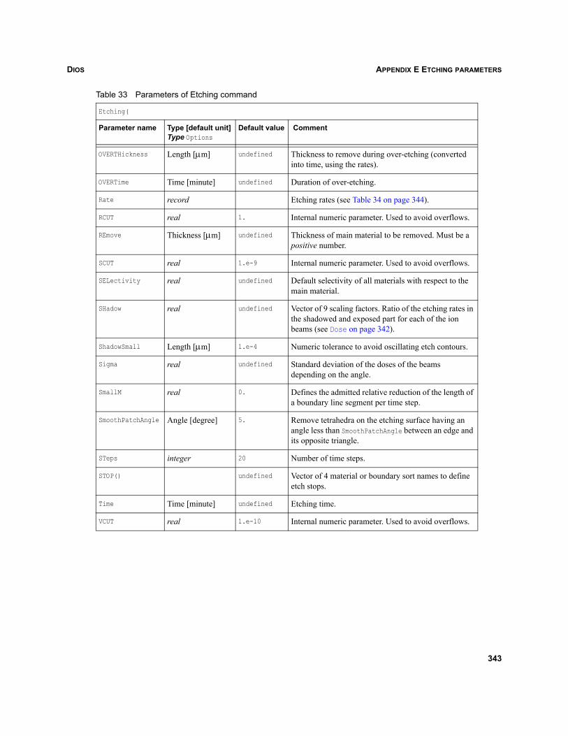
DIOS APPENDIX E ETCHING PARAMETERS
OVERTHickness Length [μm] undefined Thickness to remove during over-etching (converted into time, using the rates).
OVERTime Time [minute] undefined Duration of over-etching.
Rate record Etching rates (see Table 34 on page 344).
RCUT real 1. Internal numeric parameter. Used to avoid overflows.
REmove Thickness [μm] undefined Thickness of main material to be removed. Must be a positive number.
SCUT real 1.e-9 Internal numeric parameter. Used to avoid overflows.
SELectivity real undefined Default selectivity of all materials with respect to the main material.
SHadow real undefined Vector of 9 scaling factors. Ratio of the etching rates in the shadowed and exposed part for each of the ion beams (see Dose on page 342).
ShadowSmall Length [μm] 1.e-4 Numeric tolerance to avoid oscillating etch contours.
Sigma real undefined Standard deviation of the doses of the beams depending on the angle.
SmallM real 0. Defines the admitted relative reduction of the length of a boundary line segment per time step.
SmoothPatchAngle Angle [degree] 5. Remove tetrahedra on the etching surface having an angle less than SmoothPatchAngle between an edge and its opposite triangle.
STeps integer 20 Number of time steps.
STOP() undefined Vector of 4 material or boundary sort names to define etch stops.
Time Time [minute] undefined Etching time.
VCUT real 1.e-10 Internal numeric parameter. Used to avoid overflows.
Table 33 Parameters of Etching command
Etching(
Parameter name Type [default unit]Type Options
Default value Comment
343
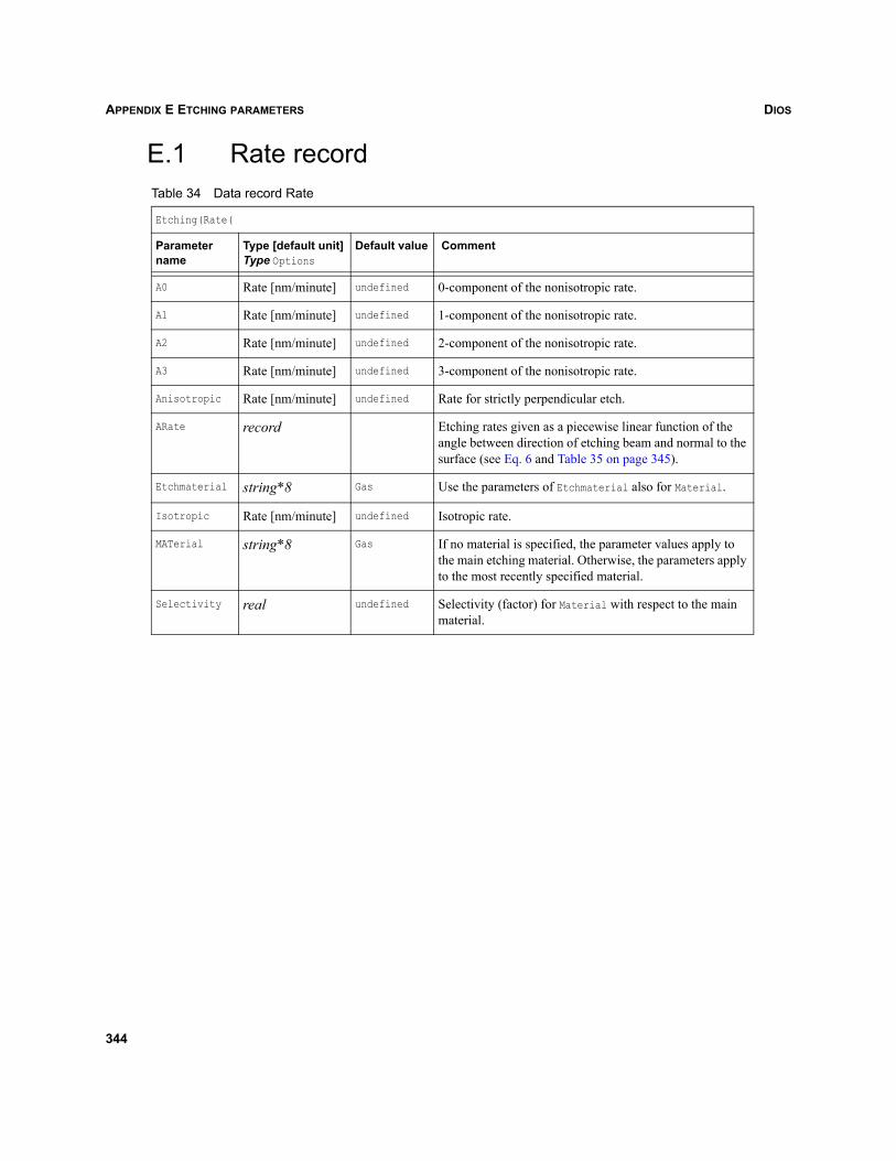
DIOSAPPENDIX E ETCHING PARAMETERS
E.1 Rate recordTable 34 Data record Rate
Etching(Rate(
Parameter name
Type [default unit]Type Options
Default value Comment
A0 Rate [nm/minute] undefined 0-component of the nonisotropic rate.
A1 Rate [nm/minute] undefined 1-component of the nonisotropic rate.
A2 Rate [nm/minute] undefined 2-component of the nonisotropic rate.
A3 Rate [nm/minute] undefined 3-component of the nonisotropic rate.
Anisotropic Rate [nm/minute] undefined Rate for strictly perpendicular etch.
ARate record Etching rates given as a piecewise linear function of the angle between direction of etching beam and normal to the surface (see Eq. 6 and Table 35 on page 345).
Etchmaterial string*8 Gas Use the parameters of Etchmaterial also for Material.
Isotropic Rate [nm/minute] undefined Isotropic rate.
MATerial string*8 Gas If no material is specified, the parameter values apply to the main etching material. Otherwise, the parameters apply to the most recently specified material.
Selectivity real undefined Selectivity (factor) for Material with respect to the main material.
344
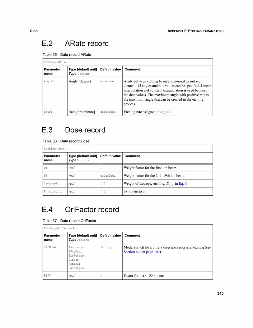
DIOS APPENDIX E ETCHING PARAMETERS
E.2 ARate record
E.3 Dose record
E.4 OriFactor record
Table 35 Data record ARate
Etching(ARate(
Parameter name
Type [default unit]Type Options
Default value Comment
Angle1 Angle [degree] undefined Angle between etching beam and normal to surface element; 15 angles and rate values can be specified. Linear interpolation and constant extrapolation is used between the data values. The maximum angle with positive rate is the maximum angle that can be created in the etching process.
Rate1 Rate [nm/minute] undefined Etching rate assigned to Angle1.
Table 36 Data record Dose
Etching(Dose(
Parameter name
Type [default unit]Type Options
Default value Comment
D1 real 1 Weight factor for the first ion beam.
D2 real undefined Weight factor for the 2nd…9th ion beam.
Isotropic real 1.0 Weight of isotropic etching, in Eq. 6.
Anisotropic real 1.0 Synonym to D1
Table 37 Data record OriFactor
Etching(OriFactor(
Parameter name
Type [default unit]Type Options
Default value Comment
ORIMode IsotropicSProductProjectionLinearCUbicalHalfAngle
Isotropic Model switch for arbitrary directions in crystal etching (see Section 6.4 on page 104).
R100 real 1 Factor for the <100> plane.
Diso
345
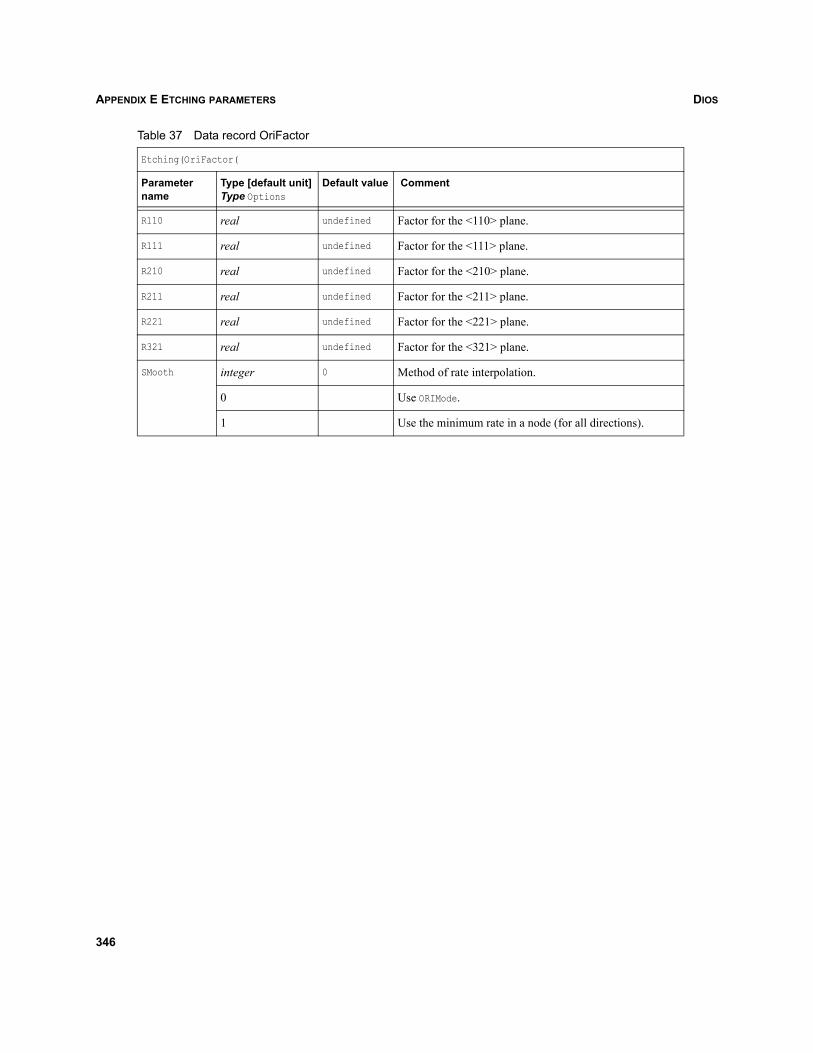
DIOSAPPENDIX E ETCHING PARAMETERS
R110 real undefined Factor for the <110> plane.
R111 real undefined Factor for the <111> plane.
R210 real undefined Factor for the <210> plane.
R211 real undefined Factor for the <211> plane.
R221 real undefined Factor for the <221> plane.
R321 real undefined Factor for the <321> plane.
SMooth integer 0 Method of rate interpolation.
0 Use ORIMode.
1 Use the minimum rate in a node (for all directions).
Table 37 Data record OriFactor
Etching(OriFactor(
Parameter name
Type [default unit]Type Options
Default value Comment
346
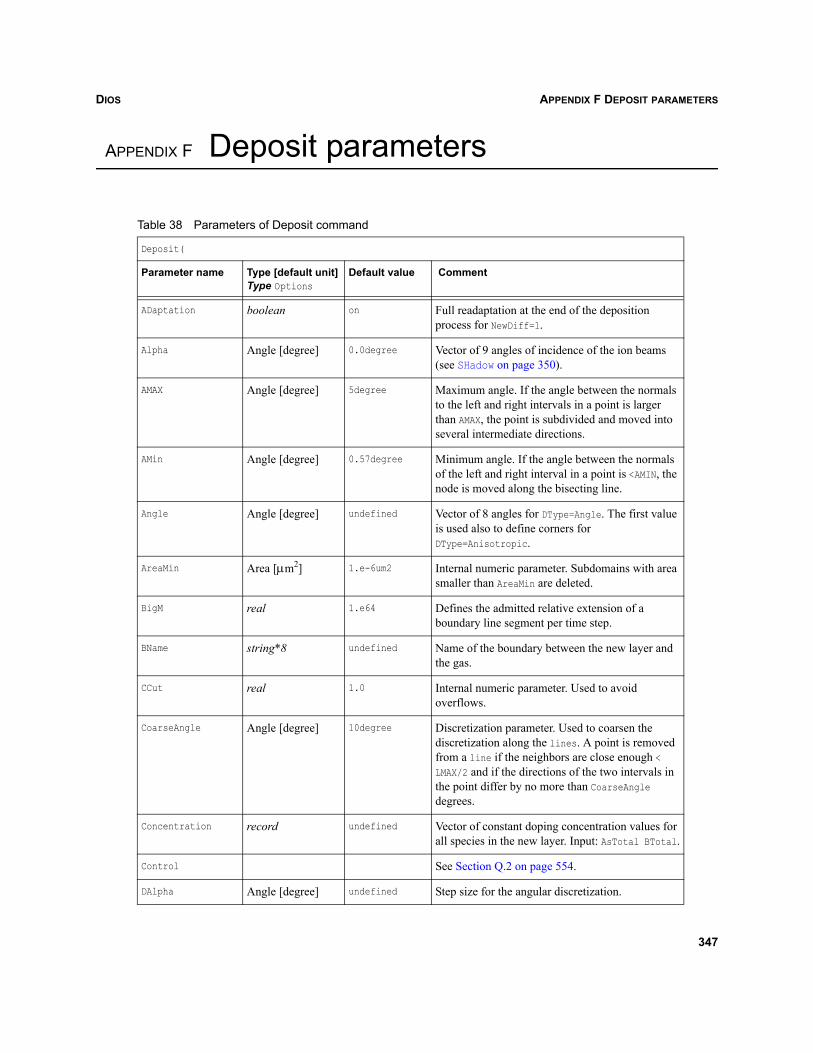
DIOS APPENDIX F DEPOSIT PARAMETERS
Dios
APPENDIX F Deposit parameters
Table 38 Parameters of Deposit command
Deposit(
Parameter name Type [default unit]Type Options
Default value Comment
ADaptation boolean on Full readaptation at the end of the deposition process for NewDiff=1.
Alpha Angle [degree] 0.0degree Vector of 9 angles of incidence of the ion beams (see SHadow on page 350).
AMAX Angle [degree] 5degree Maximum angle. If the angle between the normals to the left and right intervals in a point is larger than AMAX, the point is subdivided and moved into several intermediate directions.
AMin Angle [degree] 0.57degree Minimum angle. If the angle between the normals of the left and right interval in a point is <AMIN, the node is moved along the bisecting line.
Angle Angle [degree] undefined Vector of 8 angles for DType=Angle. The first value is used also to define corners for DType=Anisotropic.
AreaMin Area [μm2] 1.e-6um2 Internal numeric parameter. Subdomains with area smaller than AreaMin are deleted.
BigM real 1.e64 Defines the admitted relative extension of a boundary line segment per time step.
BName string*8 undefined Name of the boundary between the new layer and the gas.
CCut real 1.0 Internal numeric parameter. Used to avoid overflows.
CoarseAngle Angle [degree] 10degree Discretization parameter. Used to coarsen the discretization along the lines. A point is removed from a line if the neighbors are close enough < LMAX/2 and if the directions of the two intervals in the point differ by no more than CoarseAngle degrees.
Concentration record undefined Vector of constant doping concentration values for all species in the new layer. Input: AsTotal BTotal.
Control See Section Q.2 on page 554.
DAlpha Angle [degree] undefined Step size for the angular discretization.
347
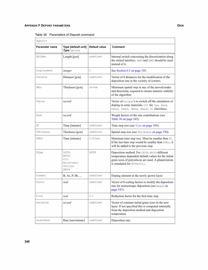
DIOSAPPENDIX F DEPOSIT PARAMETERS
DELCMax Length [μm] undefined Internal switch concerning the discretization along the etched interface. LMIN and LMAX should be used instead of it.
Displacement integer 2 See Section 6.5 on page 105.
DIstance Distance [μm] undefined Vector of 8 distances for the modification of the deposition rate in the vicinity of corners.
DMin Thickness [μm] 1e-9um Minimum spatial step in any of the moved nodes and directions, required to ensure numeric stability of the algorithm.
Doping record Vector of boolean’s to switch off the simulation of doping in some materials. Off for Gas, Rand, ORand, LRand, URand, RRand; On elsewhere.
Dose record Weight factors of the rate contributions (see Table 36 on page 345).
DT Time [minute] undefined Time step size (see Time on page 350).
DTHickness Thickness [μm] undefined Spatial step size (see THickness on page 350).
DTMin Time [minute] 0.001min Minimum time step size. Must be smaller than DT. If the last time step would be smaller than DTMin, it will be added to the previous step.
DType LPCVDNPCVDFillAnisotropicVerticalANGle
LPCVD Deposition method. For LPCVD, NPCVD different temperature dependent default values for the initial grain sizes of polysilicon are used. A planarization is simulated for DTYPe=Fill.
Element B, As, P, Sb, ... undefined Doping element in the newly grown layer.
Factor real undefined Vector of 8 scaling factors to modify the deposition rate for nonisotropic deposition (see Angle on page 347).
First real 0.1 Reduction factor for the first time step.
GrainSize record undefined Vector of constant initial grain sizes in the new layer. If not specified this is computed internally from the deposition method and deposition temperature.
GrowthRate Rate [nm/minute] undefined Deposition rate.
Table 38 Parameters of Deposit command
Deposit(
Parameter name Type [default unit]Type Options
Default value Comment
348
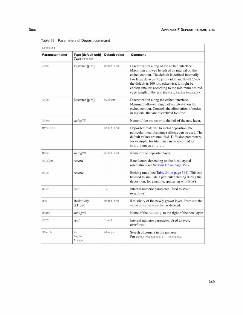
DIOS APPENDIX F DEPOSIT PARAMETERS
LMAX Distance [μm] undefined Discretization along of the etched interface. Maximum allowed length of an interval on the etched contour. The default is defined internally. For large devices (>3 μm width, and NewDiff=0) the default is 100 nm, otherwise, it might be chosen smaller, according to the minimum desired edge length in the grid (Maxtrl, RefineBoundary).
LMIN Distance [μm] 0.001um Discretization along the etched interface. Minimum allowed length of an interval on the etched contour. Controls the elimination of nodes in regions, that are discretized too fine.
LName string*8 Name of the boundary to the left of the new layer.
MATerial undefined Deposited material. In metal deposition, the particular metal forming a silicide can be used. The default values are modified. Diffusion parameters, for example, for titanium can be specified as ME(...) not as TI(...).
Name string*8 undefined Name of the deposited layer.
ORIfact record Rate factors depending on the local crystal orientation (see Section F.2 on page 352).
Rate record Etching rates (see Table 34 on page 344). This can be used to simulate a particular etching during the deposition, for example, sputtering with BIAS.
RCUT real 1. Internal numeric parameter. Used to avoid overflows.
RHO Resistivity [ cm]
undefined Resistivity of the newly grown layer. From RHO the value of Concentration is defined.
RName string*8 Name of the boundary to the right of the new layer.
SCUT real 1.e-9 Internal numeric parameter. Used to avoid overflows.
SEarch NoBeginAlways
Always Search of corners in the gas area.For DType=Anisotropic | Vertical.
Table 38 Parameters of Deposit command
Deposit(
Parameter name Type [default unit]Type Options
Default value Comment
Ω
349
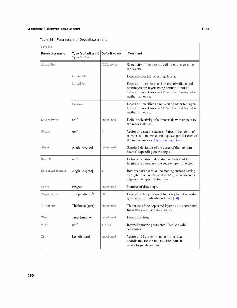
DIOSAPPENDIX F DEPOSIT PARAMETERS
Selection AllDepoMat Selectivity of the deposit with regard to existing top layers.
AllDepoMat Deposit Material on all top layers.
OnlySiPo Deposit Si on silicon and Po on polysilicon and nothing on top layers being neither Si nor Po. Selection is set back to AllDepoMat if Material is neither Si nor Po.
AllSiPo Deposit Si on silicon and Po on all other top layers. Selection is set back to AllDepoMat if MATerial is neither Si nor Po.
SELectivity real undefined Default selectivity of all materials with respect to the main material.
SHadow real 0. Vector of 9 scaling factors. Ratio of the ‘etching’ rates in the shadowed and exposed part for each of the ion beams (see Alpha on page 347).
Sigma Angle [degree] undefined Standard deviation of the doses of the ‘etching beams’ depending on the angle.
SmallM real 0. Defines the admitted relative reduction of the length of a boundary line segment per time step.
SmoothPatchAngle Angle [degree] 5. Remove tetrahedra on the etching surface having an angle less than SmoothPatchAngle between an edge and its opposite triangle.
STeps integer undefined Number of time steps.
Temperature Temperature [oC] 600. Deposition temperature. Used only to define initial grain sizes for polysilicon layers [19].
THickness Thickness [μm] undefined Thickness of the deposited layer. Time is computed from THickness and GrowthRate.
Time Time [minute] undefined Deposition time.
VCUT real 1.e-10 Internal numeric parameter. Used to avoid overflows.
XYz Length [μm] undefined Vector of 20 corner points or 40 vertical coordinates for the rate modifications in nonisotropic deposition.
Table 38 Parameters of Deposit command
Deposit(
Parameter name Type [default unit]Type Options
Default value Comment
350
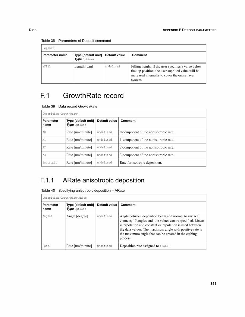
DIOS APPENDIX F DEPOSIT PARAMETERS
F.1 GrowthRate record
F.1.1 ARate anisotropic deposition
YFill Length [μm] undefined Filling height. If the user specifies a value below the top position, the user supplied value will be increased internally to cover the entire layer system.
Table 39 Data record GrowthRate
Deposition(GrowthRate(
Parameter name
Type [default unit]Type Options
Default value Comment
A0 Rate [nm/minute] undefined 0-component of the nonisotropic rate.
A1 Rate [nm/minute] undefined 1-component of the nonisotropic rate.
A2 Rate [nm/minute] undefined 2-component of the nonisotropic rate.
A3 Rate [nm/minute] undefined 3-component of the nonisotropic rate.
isotropic Rate [nm/minute] undefined Rate for isotropic deposition.
Table 40 Specifying anisotropic deposition – ARate
Deposition(GrowthRate(ARate
Parameter name
Type [default unit]Type Options
Default value Comment
Angle1 Angle [degree] undefined Angle between deposition beam and normal to surface element; 15 angles and rate values can be specified. Linear interpolation and constant extrapolation is used between the data values. The maximum angle with positive rate is the maximum angle that can be created in the etching process.
Rate1 Rate [nm/minute] undefined Deposition rate assigned to Angle1.
Table 38 Parameters of Deposit command
Deposit(
Parameter name Type [default unit]Type Options
Default value Comment
351
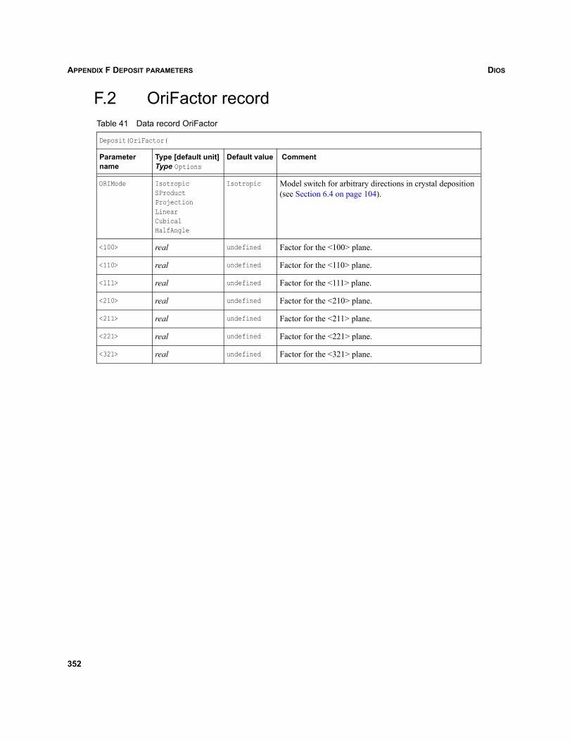
DIOSAPPENDIX F DEPOSIT PARAMETERS
F.2 OriFactor recordTable 41 Data record OriFactor
Deposit(OriFactor(
Parameter name
Type [default unit]Type Options
Default value Comment
ORIMode IsotropicSProductProjectionLinearCubicalHalfAngle
Isotropic Model switch for arbitrary directions in crystal deposition (see Section 6.4 on page 104).
<100> real undefined Factor for the <100> plane.
<110> real undefined Factor for the <110> plane.
<111> real undefined Factor for the <111> plane.
<210> real undefined Factor for the <210> plane.
<211> real undefined Factor for the <211> plane.
<221> real undefined Factor for the <221> plane.
<321> real undefined Factor for the <321> plane.
352
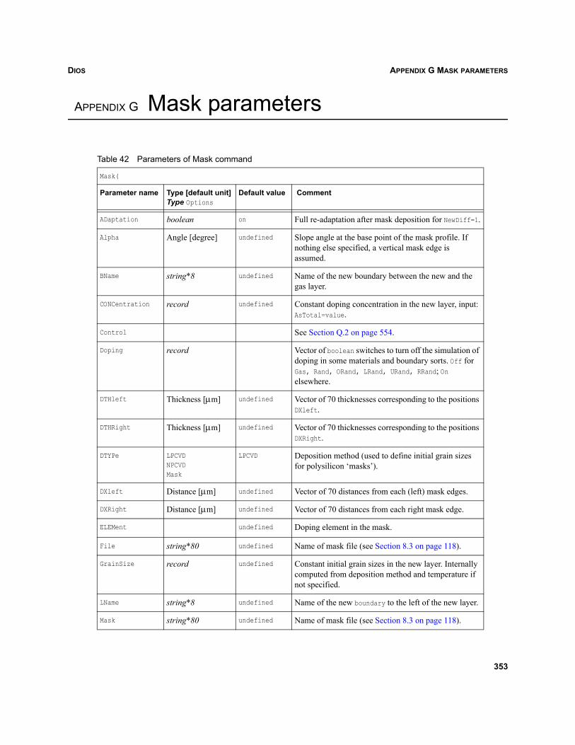
DIOS APPENDIX G MASK PARAMETERS
Dios
APPENDIX G Mask parameters
Table 42 Parameters of Mask command
Mask(
Parameter name Type [default unit]Type Options
Default value Comment
ADaptation boolean on Full re-adaptation after mask deposition for NewDiff=1.
Alpha Angle [degree] undefined Slope angle at the base point of the mask profile. If nothing else specified, a vertical mask edge is assumed.
BName string*8 undefined Name of the new boundary between the new and the gas layer.
CONCentration record undefined Constant doping concentration in the new layer, input: AsTotal=value.
Control See Section Q.2 on page 554.
Doping record Vector of boolean switches to turn off the simulation of doping in some materials and boundary sorts. Off for Gas, Rand, ORand, LRand, URand, RRand; On elsewhere.
DTHleft Thickness [μm] undefined Vector of 70 thicknesses corresponding to the positions DXleft.
DTHRight Thickness [μm] undefined Vector of 70 thicknesses corresponding to the positions DXRight.
DTYPe LPCVDNPCVDMask
LPCVD Deposition method (used to define initial grain sizes for polysilicon ‘masks’).
DXleft Distance [μm] undefined Vector of 70 distances from each (left) mask edges.
DXRight Distance [μm] undefined Vector of 70 distances from each right mask edge.
ELEMent undefined Doping element in the mask.
File string*80 undefined Name of mask file (see Section 8.3 on page 118).
GrainSize record undefined Constant initial grain sizes in the new layer. Internally computed from deposition method and temperature if not specified.
LName string*8 undefined Name of the new boundary to the left of the new layer.
Mask string*80 undefined Name of mask file (see Section 8.3 on page 118).
353
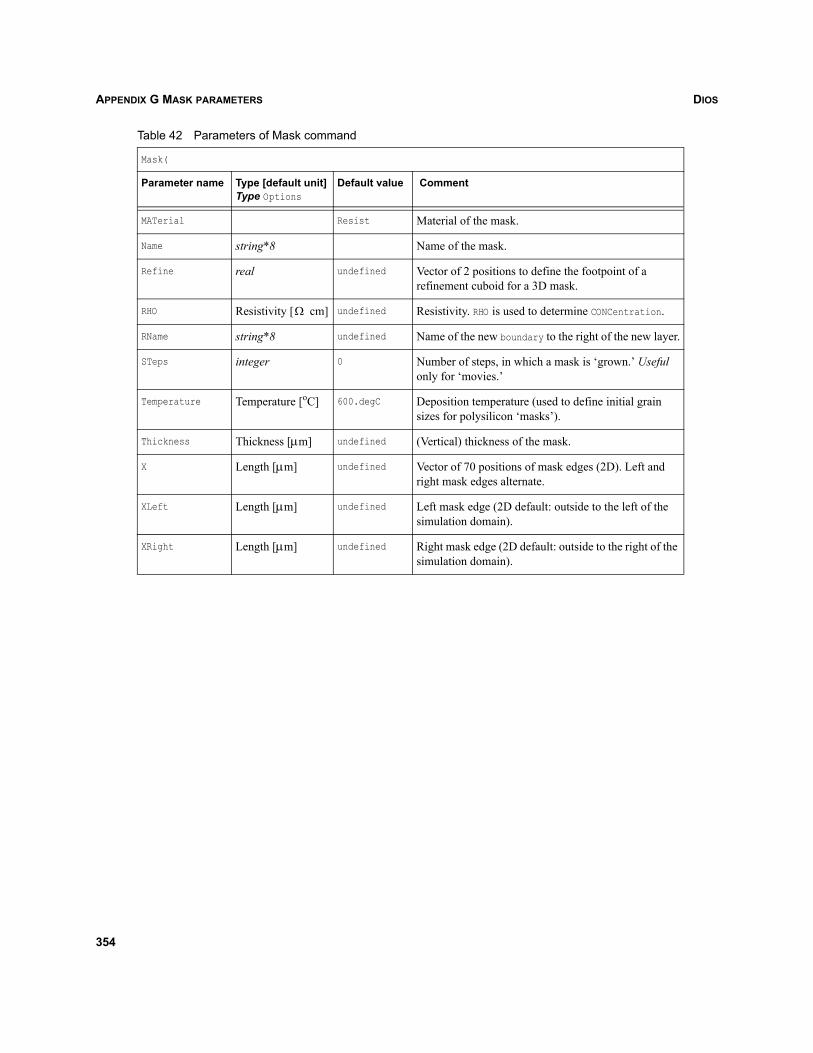
DIOSAPPENDIX G MASK PARAMETERS
MATerial Resist Material of the mask.
Name string*8 Name of the mask.
Refine real undefined Vector of 2 positions to define the footpoint of a refinement cuboid for a 3D mask.
RHO Resistivity [ cm] undefined Resistivity. RHO is used to determine CONCentration.
RName string*8 undefined Name of the new boundary to the right of the new layer.
STeps integer 0 Number of steps, in which a mask is ‘grown.’ Useful only for ‘movies.’
Temperature Temperature [oC] 600.degC Deposition temperature (used to define initial grain sizes for polysilicon ‘masks’).
Thickness Thickness [μm] undefined (Vertical) thickness of the mask.
X Length [μm] undefined Vector of 70 positions of mask edges (2D). Left and right mask edges alternate.
XLeft Length [μm] undefined Left mask edge (2D default: outside to the left of the simulation domain).
XRight Length [μm] undefined Right mask edge (2D default: outside to the right of the simulation domain).
Table 42 Parameters of Mask command
Mask(
Parameter name Type [default unit]Type Options
Default value Comment
Ω
354
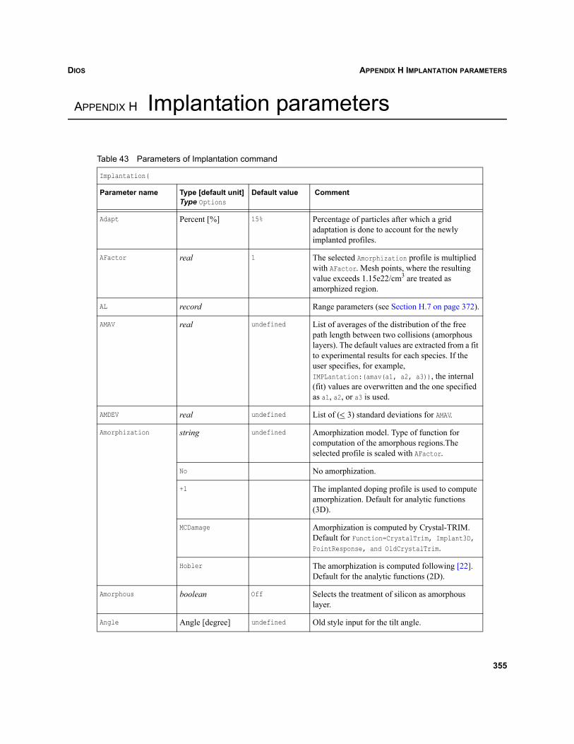
DIOS APPENDIX H IMPLANTATION PARAMETERS
Dios
APPENDIX H Implantation parameters
Table 43 Parameters of Implantation command
Implantation(
Parameter name Type [default unit]Type Options
Default value Comment
Adapt Percent [%] 15% Percentage of particles after which a grid adaptation is done to account for the newly implanted profiles.
AFactor real 1 The selected Amorphization profile is multiplied with AFactor. Mesh points, where the resulting value exceeds 1.15e22/cm3 are treated as amorphized region.
AL record Range parameters (see Section H.7 on page 372).
AMAV real undefined List of averages of the distribution of the free path length between two collisions (amorphous layers). The default values are extracted from a fit to experimental results for each species. If the user specifies, for example, IMPLantation:(amav(a1, a2, a3)), the internal (fit) values are overwritten and the one specified as a1, a2, or a3 is used.
AMDEV real undefined List of (< 3) standard deviations for AMAV.
Amorphization string undefined Amorphization model. Type of function for computation of the amorphous regions.The selected profile is scaled with AFactor.
No No amorphization.
+1 The implanted doping profile is used to compute amorphization. Default for analytic functions (3D).
MCDamage Amorphization is computed by Crystal-TRIM.Default for Function=CrystalTrim, Implant3D, PointResponse, and OldCrystalTrim.
Hobler The amorphization is computed following [22]. Default for the analytic functions (2D).
Amorphous boolean Off Selects the treatment of silicon as amorphous layer.
Angle Angle [degree] undefined Old style input for the tilt angle.
355
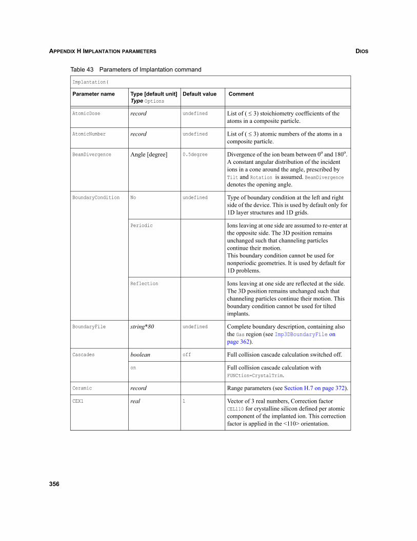
DIOSAPPENDIX H IMPLANTATION PARAMETERS
AtomicDose record undefined List of ( ) stoichiometry coefficients of the atoms in a composite particle.
AtomicNumber record undefined List of ( ) atomic numbers of the atoms in a composite particle.
BeamDivergence Angle [degree] 0.5degree Divergence of the ion beam between 0o and 180o. A constant angular distribution of the incident ions in a cone around the angle, prescribed by Tilt and Rotation is assumed. BeamDivergence denotes the opening angle.
BoundaryCondition No undefined Type of boundary condition at the left and right side of the device. This is used by default only for 1D layer structures and 1D grids.
Periodic Ions leaving at one side are assumed to re-enter at the opposite side. The 3D position remains unchanged such that channeling particles continue their motion.This boundary condition cannot be used for nonperiodic geometries. It is used by default for 1D problems.
Reflection Ions leaving at one side are reflected at the side. The 3D position remains unchanged such that channeling particles continue their motion. This boundary condition cannot be used for tilted implants.
BoundaryFile string*80 undefined Complete boundary description, containing also the Gas region (see Imp3DBoundaryFile on page 362).
Cascades boolean off Full collision cascade calculation switched off.
on Full collision cascade calculation with FUNCtion=CrystalTrim.
Ceramic record Range parameters (see Section H.7 on page 372).
CEX1 real 1 Vector of 3 real numbers, Correction factor CEL110 for crystalline silicon defined per atomic component of the implanted ion. This correction factor is applied in the <110> orientation.
Table 43 Parameters of Implantation command
Implantation(
Parameter name Type [default unit]Type Options
Default value Comment
3≤
3≤
356
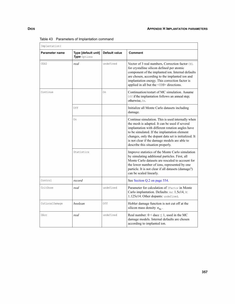
DIOS APPENDIX H IMPLANTATION PARAMETERS
CEX2 real undefined Vector of 3 real numbers, Correction factor CEL for crystalline silicon defined per atomic component of the implanted ion. Internal defaults are chosen, according to the implanted ion and implantation energy. This correction factor is applied in all but the <110> directions.
Continue On Continuation/restart of MC simulation. Assume Off if the implantation follows an anneal step; otherwise, On.
Off Initialize all Monte Carlo datasets including damage.
On Continue simulation. This is used internally when the mesh is adapted. It can be used if several implantation with different rotation angles have to be simulated. If the implantation element changes, only the dopant data set is initialized. It is not clear if the damage models are able to describe this situation properly.
Statistics Improve statistics of the Monte Carlo simulation by simulating additional particles. First, all Monte Carlo datasets are rescaled to account for the lower number of ions, represented by one particle. It is not clear if all datasets (damage?) can be scaled linearly.
Control record See Section Q.2 on page 554.
CritDose real undefined Parameter for calculation of IFactor in Monte Carlo implantation. Defaults: As: 1.5e14, B: 1.125e14. Other dopants: undefined.
CutLocalDamage boolean Off Hobler damage function is not cut off at the silicon mass density .
DAcc real undefined Real number: 0 < dacc < 1, used in the MC damage models. Internal defaults are chosen according to implanted ion.
Table 43 Parameters of Implantation command
Implantation(
Parameter name Type [default unit]Type Options
Default value Comment
nSi
357
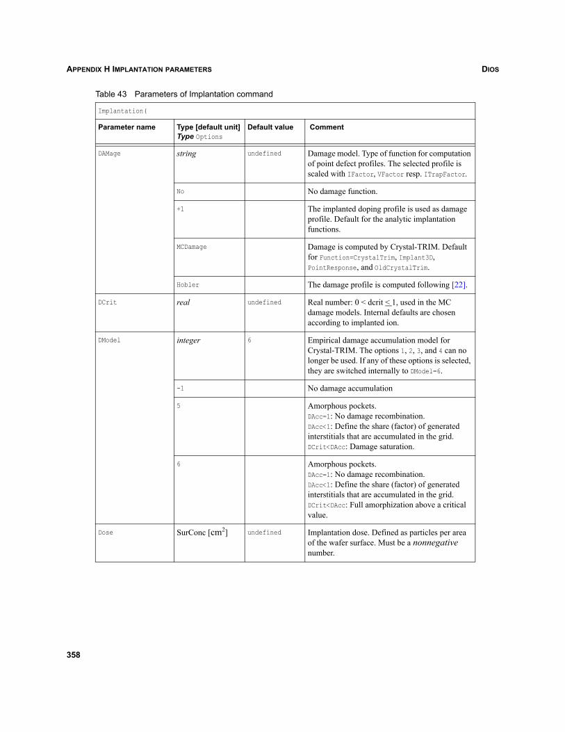
DIOSAPPENDIX H IMPLANTATION PARAMETERS
DAMage string undefined Damage model. Type of function for computation of point defect profiles. The selected profile is scaled with IFactor, VFactor resp. ITrapFactor.
No No damage function.
+1 The implanted doping profile is used as damage profile. Default for the analytic implantation functions.
MCDamage Damage is computed by Crystal-TRIM. Default for Function=CrystalTrim, Implant3D, PointResponse, and OldCrystalTrim.
Hobler The damage profile is computed following [22].
DCrit real undefined Real number: 0 < dcrit < 1, used in the MC damage models. Internal defaults are chosen according to implanted ion.
DModel integer 6 Empirical damage accumulation model for Crystal-TRIM. The options 1, 2, 3, and 4 can no longer be used. If any of these options is selected, they are switched internally to DModel=6.
-1 No damage accumulation
5 Amorphous pockets.DAcc=1: No damage recombination.DAcc<1: Define the share (factor) of generated interstitials that are accumulated in the grid.DCrit<DAcc: Damage saturation.
6 Amorphous pockets.DAcc=1: No damage recombination.DAcc<1: Define the share (factor) of generated interstitials that are accumulated in the grid.DCrit<DAcc: Full amorphization above a critical value.
Dose SurConc [cm2] undefined Implantation dose. Defined as particles per area of the wafer surface. Must be a nonnegative number.
Table 43 Parameters of Implantation command
Implantation(
Parameter name Type [default unit]Type Options
Default value Comment
358
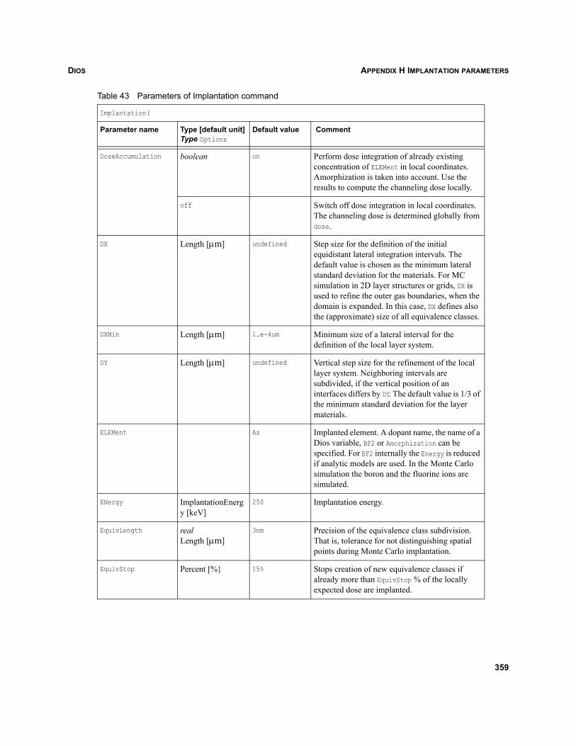
DIOS APPENDIX H IMPLANTATION PARAMETERS
DoseAccumulation boolean on Perform dose integration of already existing concentration of ELEMent in local coordinates. Amorphization is taken into account. Use the results to compute the channeling dose locally.
off Switch off dose integration in local coordinates. The channeling dose is determined globally from dose.
DX Length [μm] undefined Step size for the definition of the initial equidistant lateral integration intervals. The default value is chosen as the minimum lateral standard deviation for the materials. For MC simulation in 2D layer structures or grids, DX is used to refine the outer gas boundaries, when the domain is expanded. In this case, DX defines also the (approximate) size of all equivalence classes.
DXMin Length [μm] 1.e-4um Minimum size of a lateral interval for the definition of the local layer system.
DY Length [μm] undefined Vertical step size for the refinement of the local layer system. Neighboring intervals are subdivided, if the vertical position of an interfaces differs by DY. The default value is 1/3 of the minimum standard deviation for the layer materials.
ELEMent As Implanted element. A dopant name, the name of a Dios variable, BF2 or Amorphization can be specified. For BF2 internally the Energy is reduced if analytic models are used. In the Monte Carlo simulation the boron and the fluorine ions are simulated.
ENergy ImplantationEnergy [keV]
250 Implantation energy.
EquivLength realLength [μm]
3nm Precision of the equivalence class subdivision. That is, tolerance for not distinguishing spatial points during Monte Carlo implantation.
EquivStop Percent [%} 15% Stops creation of new equivalence classes if already more than EquivStop % of the locally expected dose are implanted.
Table 43 Parameters of Implantation command
Implantation(
Parameter name Type [default unit]Type Options
Default value Comment
359
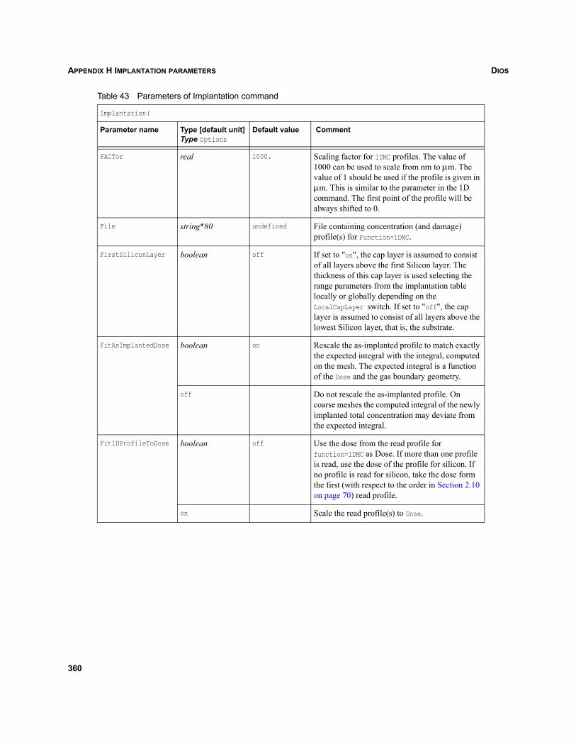
DIOSAPPENDIX H IMPLANTATION PARAMETERS
FACTor real 1000. Scaling factor for 1DMC profiles. The value of 1000 can be used to scale from nm to μm. The value of 1 should be used if the profile is given in μm. This is similar to the parameter in the 1D command. The first point of the profile will be always shifted to 0.
File string*80 undefined File containing concentration (and damage) profile(s) for Function=1DMC.
FirstSiliconLayer boolean off If set to "on", the cap layer is assumed to consist of all layers above the first Silicon layer. The thickness of this cap layer is used selecting the range parameters from the implantation table locally or globally depending on the LocalCapLayer switch. If set to "off", the cap layer is assumed to consist of all layers above the lowest Silicon layer, that is, the substrate.
FitAsImplantedDose boolean on Rescale the as-implanted profile to match exactly the expected integral with the integral, computed on the mesh. The expected integral is a function of the Dose and the gas boundary geometry.
off Do not rescale the as-implanted profile. On coarse meshes the computed integral of the newly implanted total concentration may deviate from the expected integral.
Fit1DProfileToDose boolean off Use the dose from the read profile for function=1DMC as Dose. If more than one profile is read, use the dose of the profile for silicon. If no profile is read for silicon, take the dose form the first (with respect to the order in Section 2.10 on page 70) read profile.
on Scale the read profile(s) to Dose.
Table 43 Parameters of Implantation command
Implantation(
Parameter name Type [default unit]Type Options
Default value Comment
360
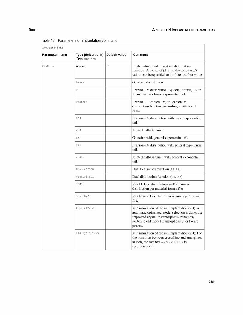
DIOS APPENDIX H IMPLANTATION PARAMETERS
FUNCtion record P4 Implantation model. Vertical distribution function. A vector of (≤ 2) of the following 8 values can be specified or 1 of the last four values
Gauss Gaussian distribution.
P4 Pearson–IV distribution. By default for B, BF2 in Si and Po with linear exponential tail.
PEarson Pearson–I, Pearson–IV, or Pearson–VI distribution function, according to GAMma and BETA.
P4S Pearson–IV distribution with linear exponential tail.
JHG Jointed half-Gaussian.
GK Gaussian with general exponential tail.
P4K Pearson–IV distribution with general exponential tail.
JHGK Jointed half-Gaussian with general exponential tail.
DualPearson Dual Pearson distribution (P4,P4).
GeneralTail Dual distribution function (P4,P4K).
1DMC Read 1D ion distribution and/or damage distribution per material from a file
Load2DMC Read one 2D ion distribution from a prf or exp file.
CrystalTrim MC simulation of the ion implantation (2D). An automatic optimized model selection is done: use improved crystalline/amorphous transition, switch to old model if amorphous Si or Po are present.
OldCrystalTrim MC simulation of the ion implantation (2D). For the transition between crystalline and amorphous silicon, the method NewCrystalTrim is recommended.
Table 43 Parameters of Implantation command
Implantation(
Parameter name Type [default unit]Type Options
Default value Comment
361
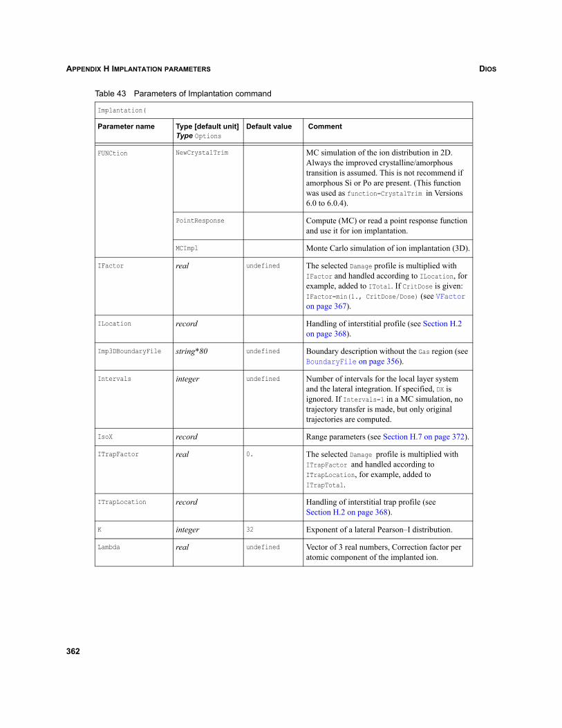
DIOSAPPENDIX H IMPLANTATION PARAMETERS
FUNCtion NewCrystalTrim MC simulation of the ion distribution in 2D. Always the improved crystalline/amorphous transition is assumed. This is not recommend if amorphous Si or Po are present. (This function was used as function=CrystalTrim in Versions 6.0 to 6.0.4).
PointResponse Compute (MC) or read a point response function and use it for ion implantation.
MCImpl Monte Carlo simulation of ion implantation (3D).
IFactor real undefined The selected Damage profile is multiplied with IFactor and handled according to ILocation, for example, added to ITotal. If CritDose is given: IFactor=min(1., CritDose/Dose) (see VFactor on page 367).
ILocation record Handling of interstitial profile (see Section H.2 on page 368).
Imp3DBoundaryFile string*80 undefined Boundary description without the Gas region (see BoundaryFile on page 356).
Intervals integer undefined Number of intervals for the local layer system and the lateral integration. If specified, DX is ignored. If Intervals=1 in a MC simulation, no trajectory transfer is made, but only original trajectories are computed.
IsoX record Range parameters (see Section H.7 on page 372).
ITrapFactor real 0. The selected Damage profile is multiplied with ITrapFactor and handled according to ITrapLocation, for example, added to ITrapTotal.
ITrapLocation record Handling of interstitial trap profile (see Section H.2 on page 368).
K integer 32 Exponent of a lateral Pearson–I distribution.
Lambda real undefined Vector of 3 real numbers, Correction factor per atomic component of the implanted ion.
Table 43 Parameters of Implantation command
Implantation(
Parameter name Type [default unit]Type Options
Default value Comment
362
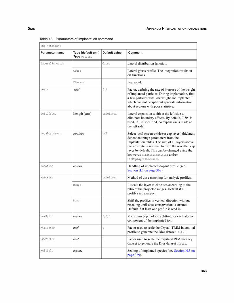
DIOS APPENDIX H IMPLANTATION PARAMETERS
LateralFunction Gauss Lateral distribution function.
Gauss Lateral gauss profile. The integration results in erf functions.
PEarson Pearson–I.
Learn real 0.1 Factor, defining the rate of increase of the weight of implanted particles. During implantation, first a few particles with low weight are implanted, which can not be split but generate information about regions with poor statistics.
LeftOffset Length [μm] undefined Lateral expansion width at the left side to eliminate boundary effects. By default, 7.5σl is used. If 0 is specified, no expansion is made at the left side.
LocalCapLayer boolean off Select local screen-oxide (or cap layer-) thickness dependent range parameters from the implantation tables. The sum of all layers above the substrate is assumed to form the so-called cap layer by default. This can be changed using the keywords FirstSiliconLayer and/or EffCapLayerThickness.
Location record Handling of implanted dopant profile (see Section H.1 on page 368).
MATCHing undefined Method of dose matching for analytic profiles.
Range Rescale the layer thicknesses according to the ratio of the projected ranges. Default if all profiles are analytic.
Dose Shift the profiles in vertical direction without rescaling until dose conservation is ensured. Default if at least one profile is read in.
MaxSplit record 8,0,0 Maximum depth of ion splitting for each atomic component of the implanted ion.
MCIFactor real 1 Factor used to scale the Crystal-TRIM interstitial profile to generate the Dios dataset ITotal.
MCVFactor real 1 Factor used to scale the Crystal-TRIM vacancy dataset to generate the Dios dataset VTotal.
Multiply record Scaling of implanted species (see Section H.3 on page 369).
Table 43 Parameters of Implantation command
Implantation(
Parameter name Type [default unit]Type Options
Default value Comment
363
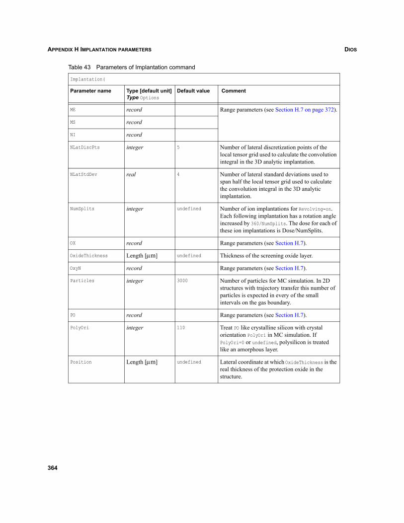
DIOSAPPENDIX H IMPLANTATION PARAMETERS
ME record Range parameters (see Section H.7 on page 372).
MS record
NI record
NLatDiscPts integer 5 Number of lateral discretization points of the local tensor grid used to calculate the convolution integral in the 3D analytic implantation.
NLatStdDev real 4 Number of lateral standard deviations used to span half the local tensor grid used to calculate the convolution integral in the 3D analytic implantation.
NumSplits integer undefined Number of ion implantations for Revolving=on. Each following implantation has a rotation angle increased by 360/NumSplits. The dose for each of these ion implantations is Dose/NumSplits.
OX record Range parameters (see Section H.7).
OxideThickness Length [μm] undefined Thickness of the screening oxide layer.
OxyN record Range parameters (see Section H.7).
Particles integer 3000 Number of particles for MC simulation. In 2D structures with trajectory transfer this number of particles is expected in every of the small intervals on the gas boundary.
PO record Range parameters (see Section H.7).
PolyOri integer 110 Treat PO like crystalline silicon with crystal orientation PolyOri in MC simulation. If PolyOri=0 or undefined, polysilicon is treated like an amorphous layer.
Position Length [μm] undefined Lateral coordinate at which OxideThickness is the real thickness of the protection oxide in the structure.
Table 43 Parameters of Implantation command
Implantation(
Parameter name Type [default unit]Type Options
Default value Comment
364
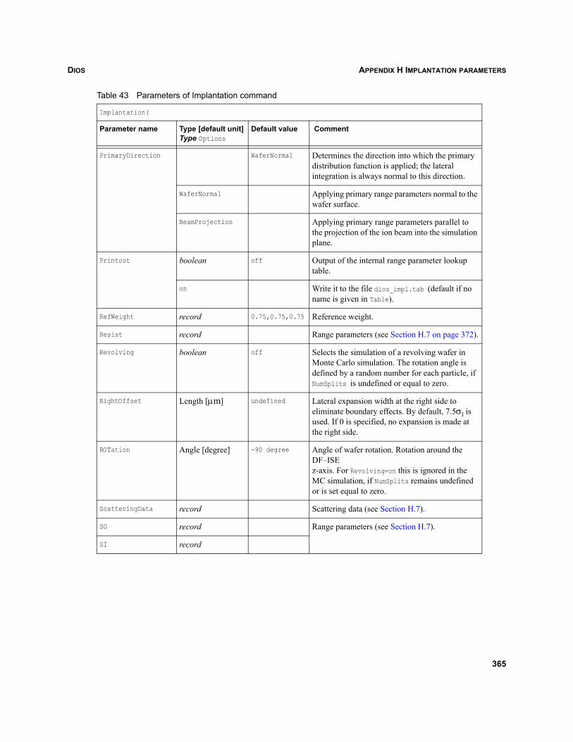
DIOS APPENDIX H IMPLANTATION PARAMETERS
PrimaryDirection WaferNormal Determines the direction into which the primary distribution function is applied; the lateral integration is always normal to this direction.
WaferNormal Applying primary range parameters normal to the wafer surface.
BeamProjection Applying primary range parameters parallel to the projection of the ion beam into the simulation plane.
Printout boolean off Output of the internal range parameter lookup table.
on Write it to the file dios_impl.tab (default if no name is given in Table).
RefWeight record 0.75,0.75,0.75 Reference weight.
Resist record Range parameters (see Section H.7 on page 372).
Revolving boolean off Selects the simulation of a revolving wafer in Monte Carlo simulation. The rotation angle is defined by a random number for each particle, if NumSplits is undefined or equal to zero.
RightOffset Length [μm] undefined Lateral expansion width at the right side to eliminate boundary effects. By default, 7.5σl is used. If 0 is specified, no expansion is made at the right side.
ROTation Angle [degree] -90 degree Angle of wafer rotation. Rotation around the DF–ISE z-axis. For Revolving=on this is ignored in the MC simulation, if NumSplits remains undefined or is set equal to zero.
ScatteringData record Scattering data (see Section H.7).
SG record Range parameters (see Section H.7).
SI record
Table 43 Parameters of Implantation command
Implantation(
Parameter name Type [default unit]Type Options
Default value Comment
365
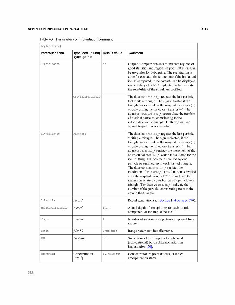
DIOSAPPENDIX H IMPLANTATION PARAMETERS
Significance No Output: Compute datasets to indicate regions of good statistics and regions of poor statistics. Can be used also for debugging. The registration is done for each atomic component of the implanted ion. If computed, these datasets can be displayed immediately after MC implantation to illustrate the reliability of the simulated profiles.
OriginalParticles The datasets ThisIon_* register the last particle that visits a triangle. The sign indicates if the triangle was visited by the original trajectory (+) or only during the trajectory transfer (–). The datasets NumberOfIons_* accumulate the number of distinct particles, contributing to the information in the triangle. Both original and copied trajectories are counted.
Significance MaxShare The datasets ThisIon_* register the last particle, visiting a triangle. The sign indicates, if the triangle was visited by the original trajectory (+) or only during the trajectory transfer (–). The datasets DeltaPLC_* register the increment of the collision counter PLC_* which is evaluated for the ion splitting. All increments caused by one particle re summed up in each visited triangle. The datasets MaxDeltaPlc_* register the maximum of DeltaPlc_*. This function is divided after the implantation by PLC_* to indicate the maximum relative contribution of a particle to a triangle. The datasets MaxIon_* indicate the number of the particle, contributing most to the data in the triangle.
SiRecoils record Recoil generation (see Section H.4 on page 370).
SplitsPerTriangle record 1,1,1 Actual depth of ion splitting for each atomic component of the implanted ion.
STeps integer 1 Number of intermediate pictures displayed for a movie.
Table file*80 undefined Range parameter data file name.
TDK boolean off Switch on/off the temporarily enhanced (conventional) boron diffusion after ion implantation [50].
Threshold Concentration [cm–3]
1.15e22/cm3 Concentration of point defects, at which amorphization starts.
Table 43 Parameters of Implantation command
Implantation(
Parameter name Type [default unit]Type Options
Default value Comment
366
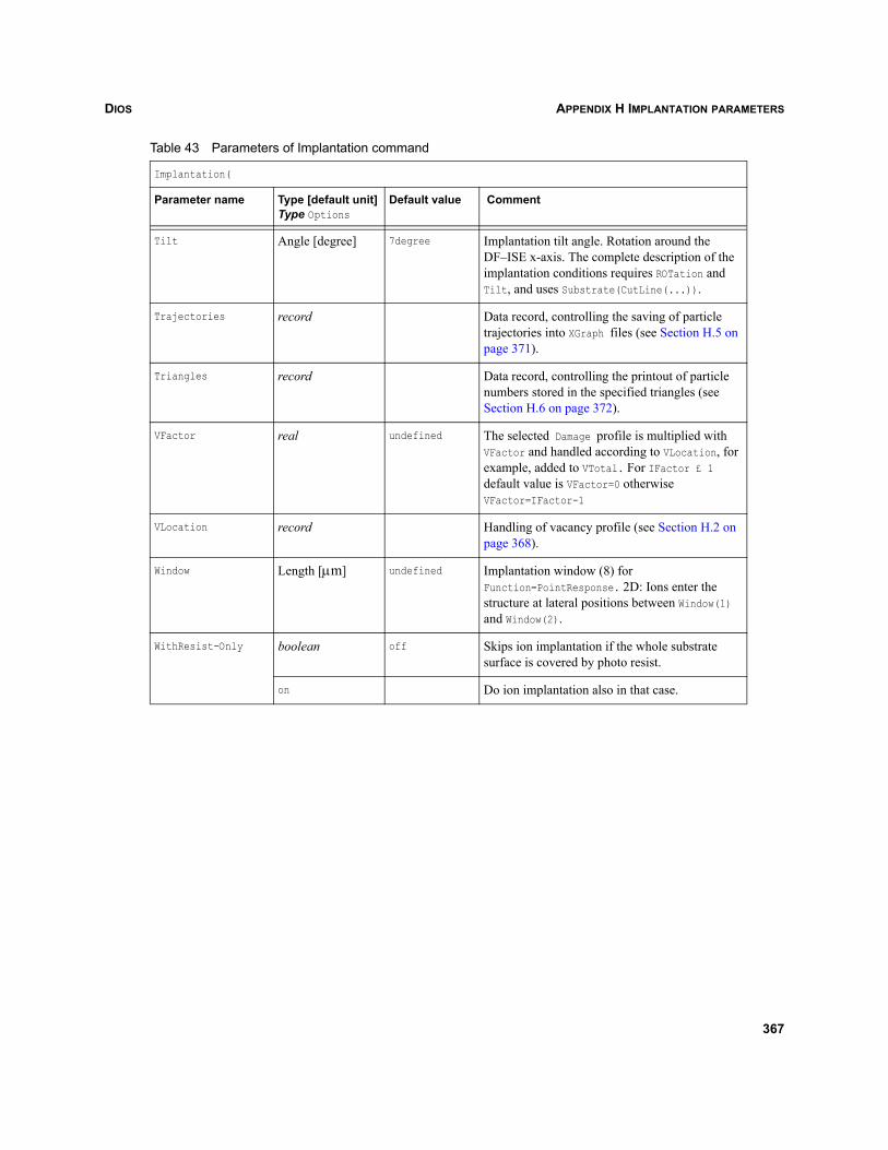
DIOS APPENDIX H IMPLANTATION PARAMETERS
Tilt Angle [degree] 7degree Implantation tilt angle. Rotation around the DF–ISE x-axis. The complete description of the implantation conditions requires ROTation and Tilt, and uses Substrate(CutLine(...)).
Trajectories record Data record, controlling the saving of particle trajectories into XGraph files (see Section H.5 on page 371).
Triangles record Data record, controlling the printout of particle numbers stored in the specified triangles (see Section H.6 on page 372).
VFactor real undefined The selected Damage profile is multiplied with VFactor and handled according to VLocation, for example, added to VTotal. For IFactor £ 1 default value is VFactor=0 otherwise VFactor=IFactor-1
VLocation record Handling of vacancy profile (see Section H.2 on page 368).
Window Length [μm] undefined Implantation window (8) for Function=PointResponse. 2D: Ions enter the structure at lateral positions between Window(1) and Window(2).
WithResist-Only boolean off Skips ion implantation if the whole substrate surface is covered by photo resist.
on Do ion implantation also in that case.
Table 43 Parameters of Implantation command
Implantation(
Parameter name Type [default unit]Type Options
Default value Comment
367

DIOSAPPENDIX H IMPLANTATION PARAMETERS
H.1 Location recordThe data record Location defines the handling of the newly implanted doping profile separately in theamorphized and nonamorphized regions.
H.2 ILocation recordThe data record ILocation specifies the handling of the total interstitial profile separately in theamorphized and nonamorphized regions. Similar data records ITrapLocation and VLocation with the samedefault values are defined for the total interstitial traps ITrapTotal and the vacancies.
Table 44 Data record Location
Implantation(Location(
Parameter name
Type [default unit]Type Options
Default value Comment
Amorphized Add Add Add the new profile to existing ones in amorphized regions.
Keep Do not modify existing profiles.
Delete Remove existing profiles.
Replace Replace existing profiles by the new one.
NonAmorphized Add Add Add the new profile to existing ones in non-amorphized regions.
Keep Do not modify existing profiles.
Delete Remove existing profiles.
Replace Replace existing profiles by the new one.
Table 45 Data record ILocation
Implantation(ILocation(
Parameter name
Type [default unit]Type Options
Default value Comment
Amorphized Add Delete Add the new profile to existing ones in amorphized regions.
Keep Do not modify existing profiles.
Delete Remove existing profiles.
Replace Replace existing profiles by the new one.
368
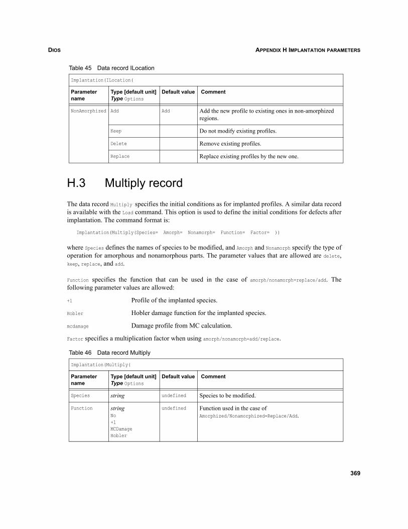
DIOS APPENDIX H IMPLANTATION PARAMETERS
H.3 Multiply recordThe data record Multiply specifies the initial conditions as for implanted profiles. A similar data recordis available with the Load command. This option is used to define the initial conditions for defects afterimplantation. The command format is:
Implantation(Multiply(Species= Amorph= Nonamorph= Function= Factor= ))
where Species defines the names of species to be modified, and Amorph and Nonamorph specify the type ofoperation for amorphous and nonamorphous parts. The parameter values that are allowed are delete,keep, replace, and add.
Function specifies the function that can be used in the case of amorph/nonamorph=replace/add. Thefollowing parameter values are allowed:
+1 Profile of the implanted species.
Hobler Hobler damage function for the implanted species.
mcdamage Damage profile from MC calculation.
Factor specifies a multiplication factor when using amorph/nonamorph=add/replace.
NonAmorphized Add Add Add the new profile to existing ones in non-amorphized regions.
Keep Do not modify existing profiles.
Delete Remove existing profiles.
Replace Replace existing profiles by the new one.
Table 46 Data record Multiply
Implantation(Multiply(
Parameter name
Type [default unit]Type Options
Default value Comment
Species string undefined Species to be modified.
Function stringNo+1MCDamageHobler
undefined Function used in the case of Amorphized/Nonamorphized=Replace/Add.
Table 45 Data record ILocation
Implantation(ILocation(
Parameter name
Type [default unit]Type Options
Default value Comment
369
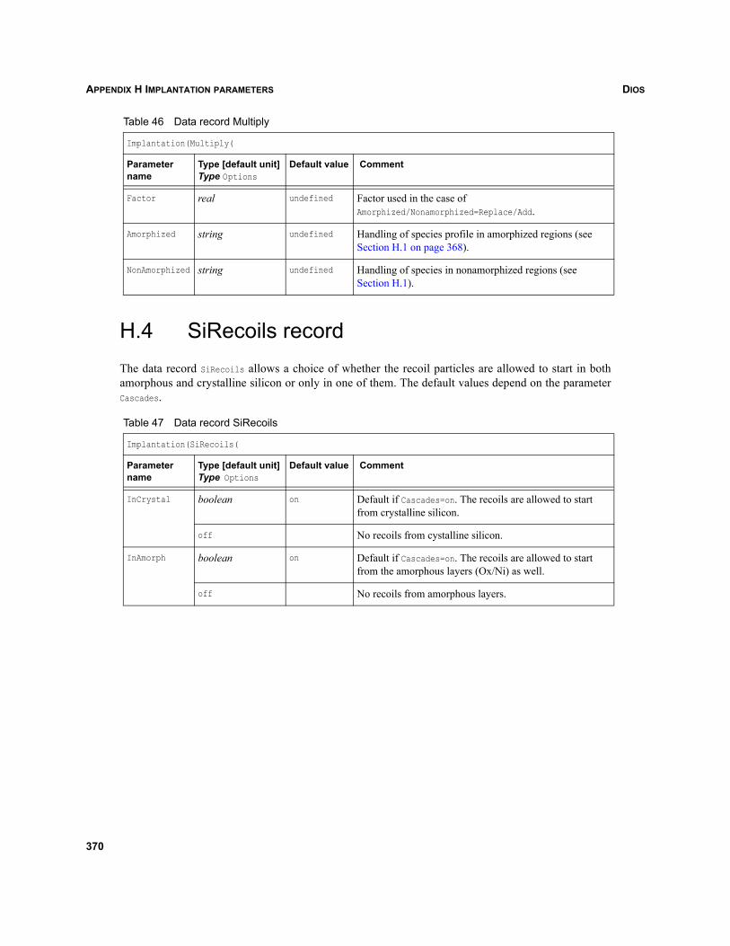
DIOSAPPENDIX H IMPLANTATION PARAMETERS
H.4 SiRecoils recordThe data record SiRecoils allows a choice of whether the recoil particles are allowed to start in bothamorphous and crystalline silicon or only in one of them. The default values depend on the parameterCascades.
Factor real undefined Factor used in the case of Amorphized/Nonamorphized=Replace/Add.
Amorphized string undefined Handling of species profile in amorphized regions (see Section H.1 on page 368).
NonAmorphized string undefined Handling of species in nonamorphized regions (see Section H.1).
Table 47 Data record SiRecoils
Implantation(SiRecoils(
Parameter name
Type [default unit]Type Options
Default value Comment
InCrystal boolean on Default if Cascades=on. The recoils are allowed to start from crystalline silicon.
off No recoils from cystalline silicon.
InAmorph boolean on Default if Cascades=on. The recoils are allowed to start from the amorphous layers (Ox/Ni) as well.
off No recoils from amorphous layers.
Table 46 Data record Multiply
Implantation(Multiply(
Parameter name
Type [default unit]Type Options
Default value Comment
370
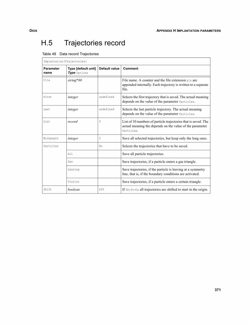
DIOS APPENDIX H IMPLANTATION PARAMETERS
H.5 Trajectories recordTable 48 Data record Trajectories
Implantation(Trajectories(
Parameter name
Type [default unit]Type Options
Default value Comment
File string*80 File name. A counter and the file extension plx are appended internally. Each trajectory is written to a separate file.
First integer undefined Selects the first trajectory that is saved. The actual meaning depends on the value of the parameter Particles.
Last integer undefined Selects the last particle trajectory. The actual meaning depends on the value of the parameter Particles.
List record 0 List of 10 numbers of particle trajectories that is saved. The actual meaning the depends on the value of the parameter Particles.
MinLength integer 2 Save all selected trajectories, but keep only the long ones.
Particles No Selects the trajectories that have to be saved.
All Save all particle trajectories.
Gas Save trajectories, if a particle enters a gas triangle.
Leaving Save trajectories, if the particle is leaving at a symmetry line, that is, if the boundary conditions are activated.
Visitor Save trajectories, if a particle enters a certain triangle.
Shift boolean Off If Shift=On all trajectories are shifted to start in the origin.
371
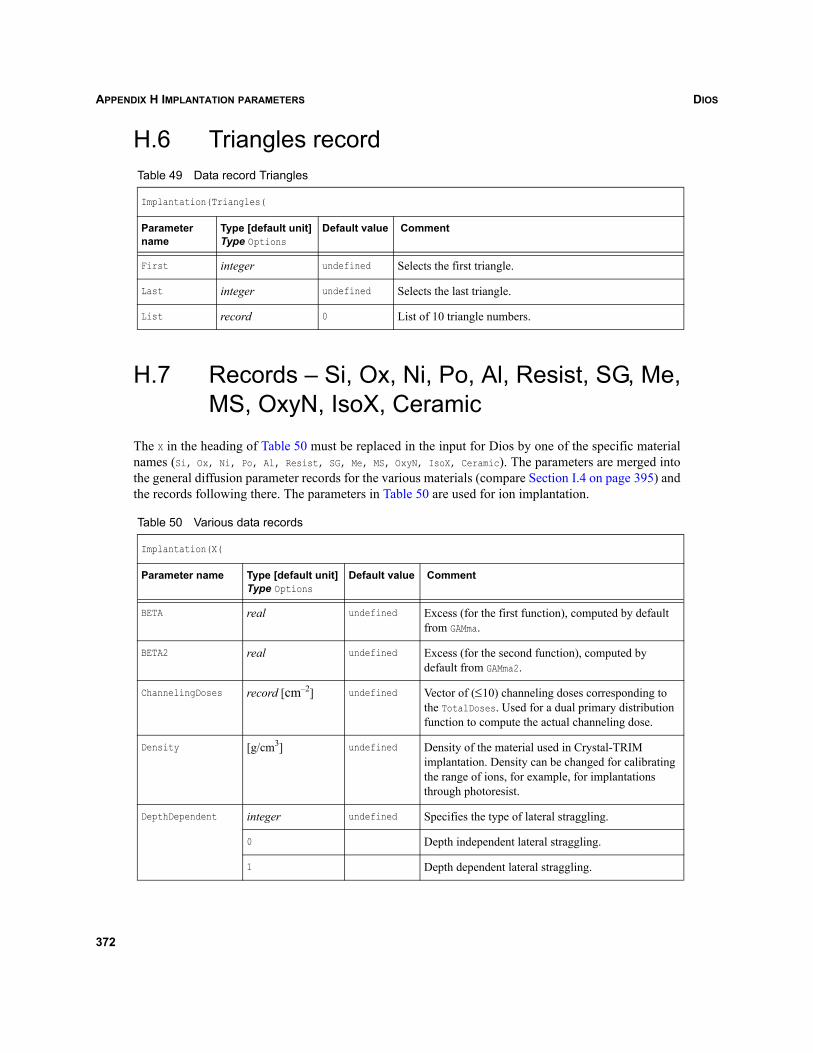
DIOSAPPENDIX H IMPLANTATION PARAMETERS
H.6 Triangles record
H.7 Records – Si, Ox, Ni, Po, Al, Resist, SG, Me, MS, OxyN, IsoX, Ceramic
The X in the heading of Table 50 must be replaced in the input for Dios by one of the specific materialnames (Si, Ox, Ni, Po, Al, Resist, SG, Me, MS, OxyN, IsoX, Ceramic). The parameters are merged intothe general diffusion parameter records for the various materials (compare Section I.4 on page 395) andthe records following there. The parameters in Table 50 are used for ion implantation.
Table 49 Data record Triangles
Implantation(Triangles(
Parameter name
Type [default unit]Type Options
Default value Comment
First integer undefined Selects the first triangle.
Last integer undefined Selects the last triangle.
List record 0 List of 10 triangle numbers.
Table 50 Various data records
Implantation(X(
Parameter name Type [default unit]Type Options
Default value Comment
BETA real undefined Excess (for the first function), computed by default from GAMma.
BETA2 real undefined Excess (for the second function), computed by default from GAMma2.
ChannelingDoses record [cm–2] undefined Vector of (≤10) channeling doses corresponding to the TotalDoses. Used for a dual primary distribution function to compute the actual channeling dose.
Density [g/cm3] undefined Density of the material used in Crystal-TRIM implantation. Density can be changed for calibrating the range of ions, for example, for implantations through photoresist.
DepthDependent integer undefined Specifies the type of lateral straggling.
0 Depth independent lateral straggling.
1 Depth dependent lateral straggling.
372
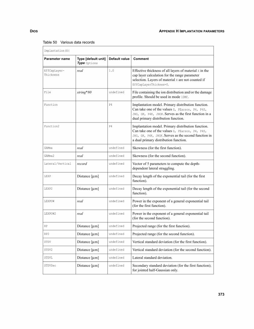
DIOS APPENDIX H IMPLANTATION PARAMETERS
EffCapLayer-Thickness
real 1.0 Effective thickness of all layers of material X in the cap layer calculation for the range parameter selection. Layers of material X are not counted if EffCapLayerThicknes=0.
File string*80 undefined File containing the ion distribution and/or the damage profile. Should be used in mode 1DMC.
Function P4 Implantation model. Primary distribution function. Can take one of the values G, PEarson, P4, P4S, JHG, GK, P4K, JHGK.Serves as the first function in a dual primary distribution function.
Function2 P4 Implantation model. Primary distribution function. Can take one of the values G, PEarson, P4, P4S, JHG, GK, P4K, JHGK.Serves as the second function in a dual primary distribution function.
GAMma real undefined Skewness (for the first function).
GAMma2 real undefined Skewness (for the second function).
Lateral/Vertical record undefined Vector of 5 parameters to compute the depth-dependent lateral straggling.
LEXP Distance [μm] undefined Decay length of the exponential tail (for the first function).
LEXP2 Distance [μm] undefined Decay length of the exponential tail (for the second function).
LEXPOW real undefined Power in the exponent of a general exponential tail (for the first function).
LEXPOW2 real undefined Power in the exponent of a general exponential tail (for the second function).
RP Distance [μm] undefined Projected range (for the first function).
RP2 Distance [μm] undefined Projected range (for the second function).
STDV Distance [μm] undefined Vertical standard deviation (for the first function).
STDV2 Distance [μm] undefined Vertical standard deviation (for the second function).
STDVL Distance [μm] undefined Lateral standard deviation.
STDVSec Distance [μm] undefined Secondary standard deviation (for the first function); for jointed half-Gaussian only.
Table 50 Various data records
Implantation(X(
Parameter name Type [default unit]Type Options
Default value Comment
373
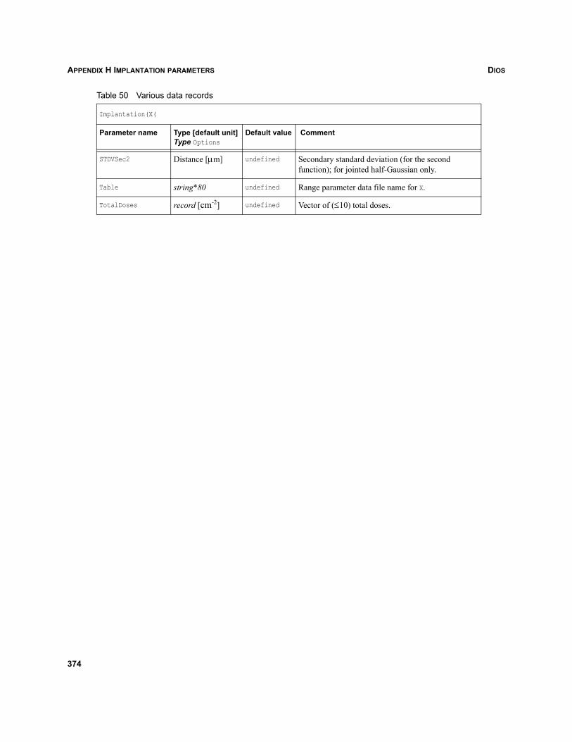
DIOSAPPENDIX H IMPLANTATION PARAMETERS
STDVSec2 Distance [μm] undefined Secondary standard deviation (for the second function); for jointed half-Gaussian only.
Table string*80 undefined Range parameter data file name for X.
TotalDoses record [cm-2] undefined Vector of (≤10) total doses.
Table 50 Various data records
Implantation(X(
Parameter name Type [default unit]Type Options
Default value Comment
374
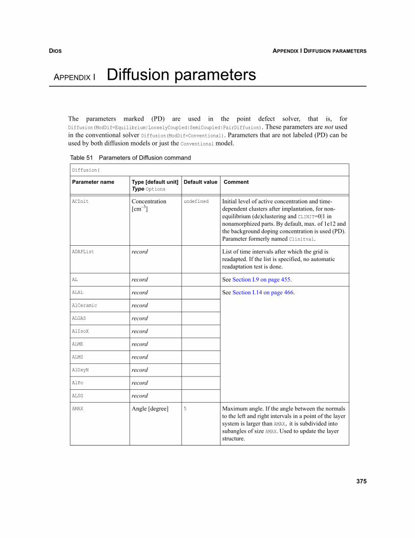
DIOS APPENDIX I DIFFUSION PARAMETERS
Dios
APPENDIX I Diffusion parameters
The parameters marked (PD) are used in the point defect solver, that is, forDiffusion(ModDif=Equilibrium|LooselyCoupled|SemiCoupled|PairDiffusion). These parameters are not usedin the conventional solver Diffusion(ModDif=Conventional). Parameters that are not labeled (PD) can beused by both diffusion models or just the Conventional model.
Table 51 Parameters of Diffusion command
Diffusion(
Parameter name Type [default unit]Type Options
Default value Comment
ACInit Concentration [cm–3]
undefined Initial level of active concentration and time-dependent clusters after implantation, for non-equilibrium (de)clustering and CLINIT=0|1 in nonamorphized parts. By default, max. of 1e12 and the background doping concentration is used (PD). Parameter formerly named Clinitval.
ADAPList record List of time intervals after which the grid is readapted. If the list is specified, no automatic readaptation test is done.
AL record See Section I.9 on page 455.
ALAL record See Section I.14 on page 466.
AlCeramic record
ALGAS record
AlIsoX record
ALME record
ALMS record
AlOxyN record
AlPo record
ALSG record
AMAX Angle [degree] 5 Maximum angle. If the angle between the normals to the left and right intervals in a point of the layer system is larger than AMAX, it is subdivided into subangles of size AMAX. Used to update the layer structure.
375
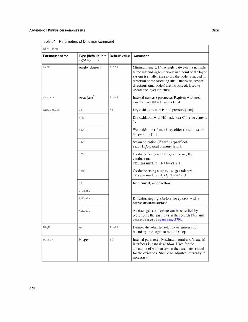
DIOSAPPENDIX I DIFFUSION PARAMETERS
AMIN Angle [degree] 0.573 Minimum angle. If the angle between the normals to the left and right intervals in a point of the layer system is smaller than AMIN, the node is moved in direction of the bisecting line. Otherwise, several directions (and nodes) are introduced. Used to update the layer structure.
AREAmin Area [μm2] 1.e-6 Internal numeric parameter. Regions with area smaller than AREAmin are deleted.
ATMOsphere O2 N2 Dry oxidation. PO2: Partial pressure [atm].
HCL Dry oxidation with HCl–add. CL: Chlorine content %.
H2O Wet oxidation (if TH2O is specified). TH2O: water temperature [oC].
H2O Steam oxidation (if PH2O is specified).PH2O: H2O partial pressure [atm].
H2O2 Oxidation using a H2:O2 gas mixture, H2 combustion.VH2: gas mixture: H2:O2=VH2:1.
H2N2 Oxidation using a H2:O2:N2 gas mixture.VH2: gas mixture: H2:O2:N2=VH2:1:1.
N2 Inert anneal, oxide reflow.
EPItaxy
PREbake Diffusion step right before the epitaxy, with a native substrate surface.
Mixture A mixed gas atmosphere can be specified by prescribing the gas flows in the records Flow and Pressure (see Flow on page 379).
BigM real 1.e64 Defines the admitted relative extension of a boundary line segment per time step.
BOUNDS integer 10 Internal parameter. Maximum number of material interfaces in a mask window. Used for the allocation of work arrays in the parameter model for the oxidation. Should be adjusted internally if necessary.
Table 51 Parameters of Diffusion command
Diffusion(
Parameter name Type [default unit]Type Options
Default value Comment
376
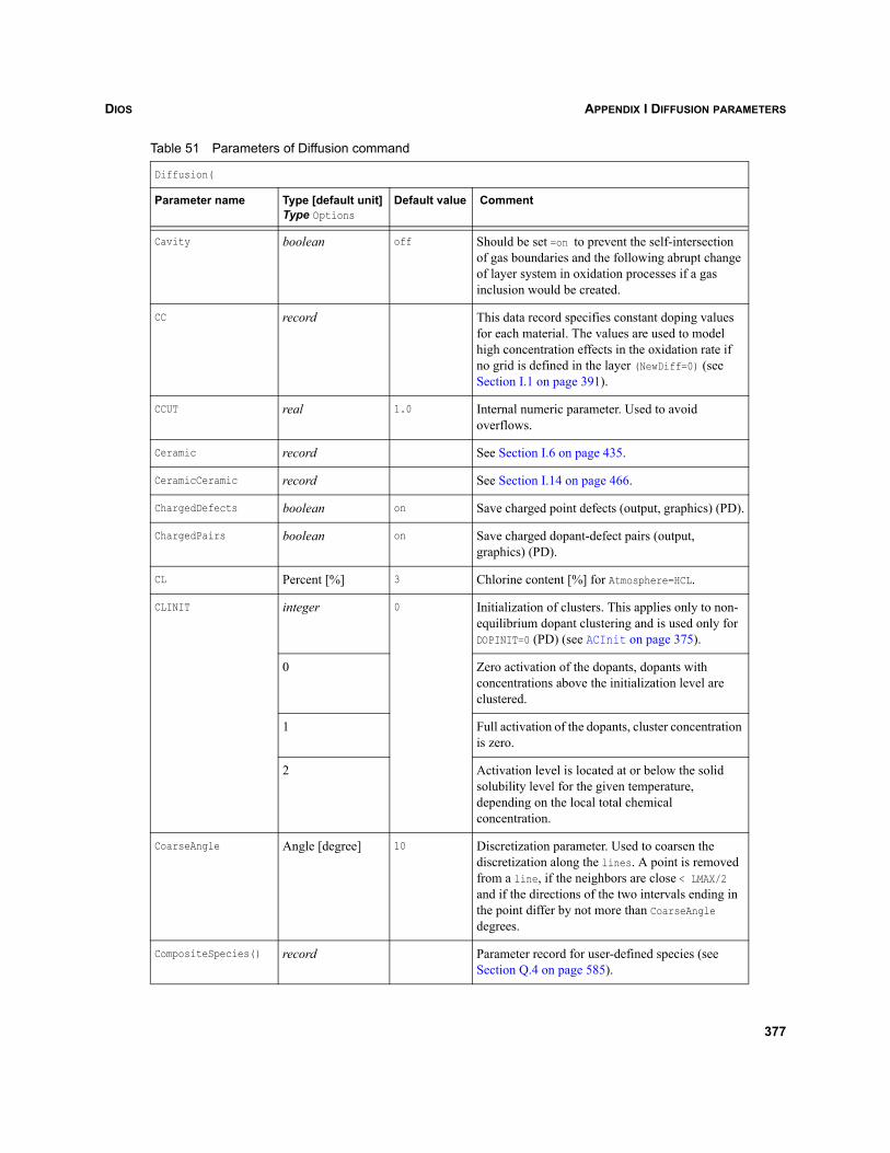
DIOS APPENDIX I DIFFUSION PARAMETERS
Cavity boolean off Should be set =on to prevent the self-intersection of gas boundaries and the following abrupt change of layer system in oxidation processes if a gas inclusion would be created.
CC record This data record specifies constant doping values for each material. The values are used to model high concentration effects in the oxidation rate if no grid is defined in the layer (NewDiff=0) (see Section I.1 on page 391).
CCUT real 1.0 Internal numeric parameter. Used to avoid overflows.
Ceramic record See Section I.6 on page 435.
CeramicCeramic record See Section I.14 on page 466.
ChargedDefects boolean on Save charged point defects (output, graphics) (PD).
ChargedPairs boolean on Save charged dopant-defect pairs (output, graphics) (PD).
CL Percent [%] 3 Chlorine content [%] for Atmosphere=HCL.
CLINIT integer 0 Initialization of clusters. This applies only to non-equilibrium dopant clustering and is used only for DOPINIT=0 (PD) (see ACInit on page 375).
0 Zero activation of the dopants, dopants with concentrations above the initialization level are clustered.
1 Full activation of the dopants, cluster concentration is zero.
2 Activation level is located at or below the solid solubility level for the given temperature, depending on the local total chemical concentration.
CoarseAngle Angle [degree] 10 Discretization parameter. Used to coarsen the discretization along the lines. A point is removed from a line, if the neighbors are close < LMAX/2 and if the directions of the two intervals ending in the point differ by not more than CoarseAngle degrees.
CompositeSpecies() record Parameter record for user-defined species (see Section Q.4 on page 585).
Table 51 Parameters of Diffusion command
Diffusion(
Parameter name Type [default unit]Type Options
Default value Comment
377
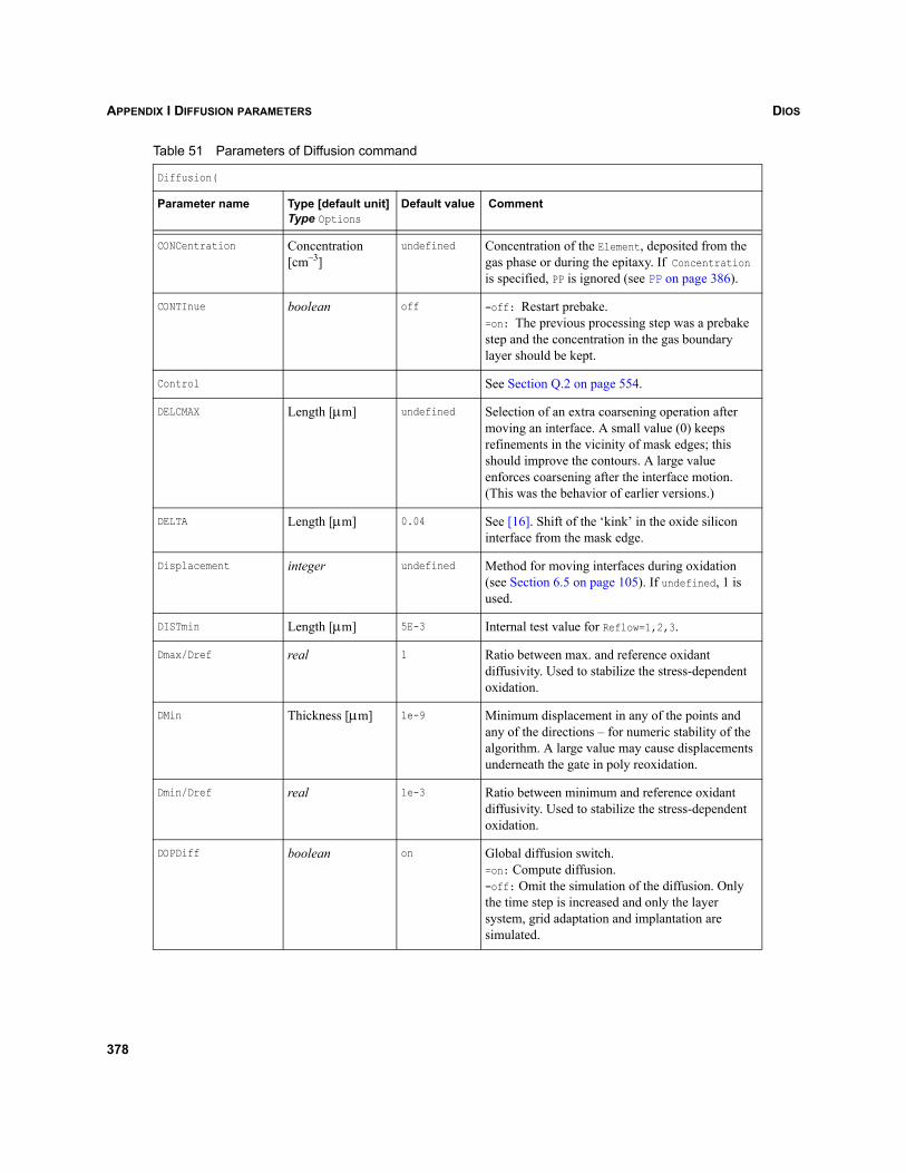
DIOSAPPENDIX I DIFFUSION PARAMETERS
CONCentration Concentration [cm–3]
undefined Concentration of the Element, deposited from the gas phase or during the epitaxy. If Concentration is specified, PP is ignored (see PP on page 386).
CONTInue boolean off =off: Restart prebake.=on: The previous processing step was a prebake step and the concentration in the gas boundary layer should be kept.
Control See Section Q.2 on page 554.
DELCMAX Length [μm] undefined Selection of an extra coarsening operation after moving an interface. A small value (0) keeps refinements in the vicinity of mask edges; this should improve the contours. A large value enforces coarsening after the interface motion. (This was the behavior of earlier versions.)
DELTA Length [μm] 0.04 See [16]. Shift of the ‘kink’ in the oxide silicon interface from the mask edge.
Displacement integer undefined Method for moving interfaces during oxidation (see Section 6.5 on page 105). If undefined, 1 is used.
DISTmin Length [μm] 5E-3 Internal test value for Reflow=1,2,3.
Dmax/Dref real 1 Ratio between max. and reference oxidant diffusivity. Used to stabilize the stress-dependent oxidation.
DMin Thickness [μm] 1e-9 Minimum displacement in any of the points and any of the directions – for numeric stability of the algorithm. A large value may cause displacements underneath the gate in poly reoxidation.
Dmin/Dref real 1e-3 Ratio between minimum and reference oxidant diffusivity. Used to stabilize the stress-dependent oxidation.
DOPDiff boolean on Global diffusion switch.=on: Compute diffusion.=off: Omit the simulation of the diffusion. Only the time step is increased and only the layer system, grid adaptation and implantation are simulated.
Table 51 Parameters of Diffusion command
Diffusion(
Parameter name Type [default unit]Type Options
Default value Comment
378
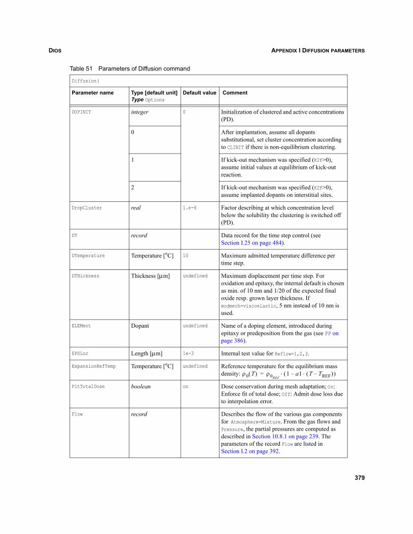
DIOS APPENDIX I DIFFUSION PARAMETERS
DOPINIT integer 0 Initialization of clustered and active concentrations (PD).
0 After implantation, assume all dopants substitutional, set cluster concentration according to CLINIT if there is non-equilibrium clustering.
1 If kick-out mechanism was specified (K2F>0), assume initial values at equilibrium of kick-out reaction.
2 If kick-out mechanism was specified (K2F>0), assume implanted dopants on interstitial sites.
DropCluster real 1.e-6 Factor describing at which concentration level below the solubility the clustering is switched off (PD).
DT record Data record for the time step control (see Section I.25 on page 484).
DTemperature Temperature [oC] 10 Maximum admitted temperature difference per time step.
DTHickness Thickness [μm] undefined Maximum displacement per time step. For oxidation and epitaxy, the internal default is chosen as min. of 10 nm and 1/20 of the expected final oxide resp. grown layer thickness. If modmech=viscoelastic, 5 nm instead of 10 nm is used.
ELEMent Dopant undefined Name of a doping element, introduced during epitaxy or predeposition from the gas (see PP on page 386).
EPSLoc Length [μm] 1e-3 Internal test value for Reflow=1,2,3.
ExpansionRefTemp Temperature [oC] undefined Reference temperature for the equilibrium mass density:
FitTotalDose boolean on Dose conservation during mesh adaptation; On: Enforce fit of total dose; Off: Admit dose loss due to interpolation error.
Flow record Describes the flow of the various gas components for Atmosphere=Mixture. From the gas flows and Pressure, the partial pressures are computed as described in Section 10.8.1 on page 239. The parameters of the record Flow are listed in Section I.2 on page 392.
Table 51 Parameters of Diffusion command
Diffusion(
Parameter name Type [default unit]Type Options
Default value Comment
ρ0 T( ) ρ0REF1 a1 T TREF–( )⋅–( )⋅=
379
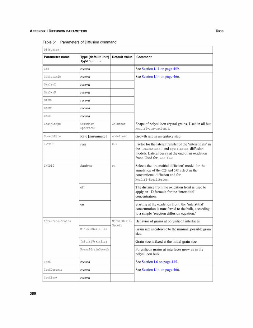
DIOSAPPENDIX I DIFFUSION PARAMETERS
Gas record See Section I.11 on page 459.
GasCeramic record See Section I.14 on page 466.
GasIsoX record
GasOxyN record
GASME record
GASMS record
GASSG record
GrainShape ColumnarSpherical
Columnar Shape of polysilicon crystal grains. Used in all but ModDiff=Conventional.
GrowthRate Rate [nm/minute] undefined Growth rate in an epitaxy step.
INTCut real 0.5 Factor for the lateral transfer of the ‘interstitials’ in the Conventional and Equilibrium diffusion models. Lateral decay at the end of an oxidation front. Used for Intdif=on.
INTDif boolean on Selects the ‘interstitial diffusion’ model for the simulation of the OED and ORD effect in the conventional diffusion and for ModDiff=Equilibrium.
off The distance from the oxidation front is used to apply an 1D formula for the ‘interstitial’ concentration.
on Starting at the oxidation front, the ‘interstitial’ concentration is transferred to the bulk, according to a simple ‘reaction diffusion equation.’
Interface-Grains NormalGrain-Growth
Behavior of grains at polysilicon interfaces
MinimumGrainSize Grain size is enforced to the minimal possible grain size.
InitialGrainSize Grain size is fixed at the initial grain size.
NormalGrainGrowth Polysilicon grains at interfaces grow as in the polysilicon bulk.
IsoX record See Section I.6 on page 435.
IsoXCeramic record See Section I.14 on page 466.
IsoXIsoX record
Table 51 Parameters of Diffusion command
Diffusion(
Parameter name Type [default unit]Type Options
Default value Comment
380
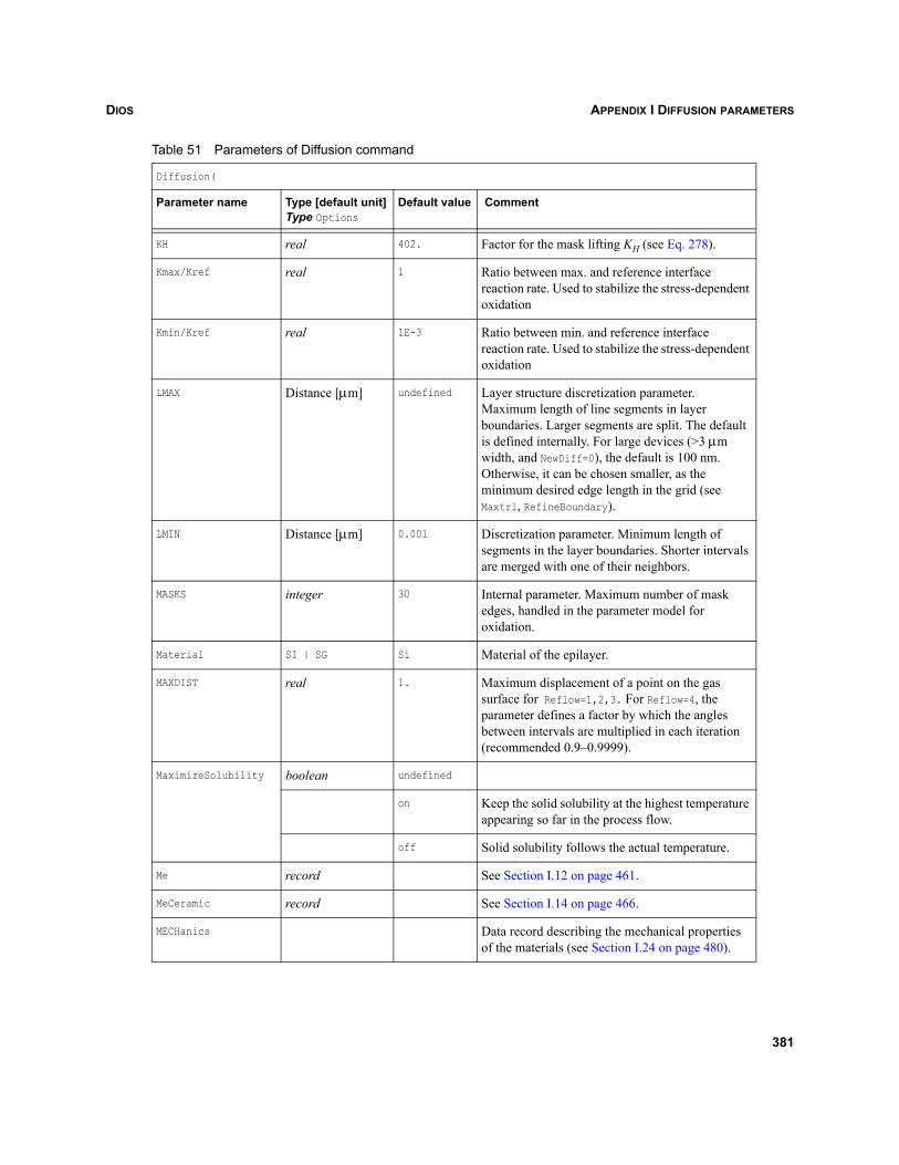
DIOS APPENDIX I DIFFUSION PARAMETERS
KH real 402. Factor for the mask lifting KH (see Eq. 278).
Kmax/Kref real 1 Ratio between max. and reference interface reaction rate. Used to stabilize the stress-dependent oxidation
Kmin/Kref real 1E-3 Ratio between min. and reference interface reaction rate. Used to stabilize the stress-dependent oxidation
LMAX Distance [μm] undefined Layer structure discretization parameter. Maximum length of line segments in layer boundaries. Larger segments are split. The default is defined internally. For large devices (>3 μm width, and NewDiff=0), the default is 100 nm. Otherwise, it can be chosen smaller, as the minimum desired edge length in the grid (see Maxtrl, RefineBoundary).
LMIN Distance [μm] 0.001 Discretization parameter. Minimum length of segments in the layer boundaries. Shorter intervals are merged with one of their neighbors.
MASKS integer 30 Internal parameter. Maximum number of mask edges, handled in the parameter model for oxidation.
Material SI | SG Si Material of the epilayer.
MAXDIST real 1. Maximum displacement of a point on the gas surface for Reflow=1,2,3. For Reflow=4, the parameter defines a factor by which the angles between intervals are multiplied in each iteration (recommended 0.9–0.9999).
MaximizeSolubility boolean undefined
on Keep the solid solubility at the highest temperature appearing so far in the process flow.
off Solid solubility follows the actual temperature.
Me record See Section I.12 on page 461.
MeCeramic record See Section I.14 on page 466.
MECHanics Data record describing the mechanical properties of the materials (see Section I.24 on page 480).
Table 51 Parameters of Diffusion command
Diffusion(
Parameter name Type [default unit]Type Options
Default value Comment
381
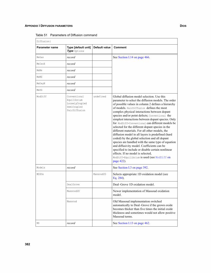
DIOSAPPENDIX I DIFFUSION PARAMETERS
MeGas record See Section I.14 on page 466.
MeIsoX record
MeMe record
MeMS record
MeOxyN record
MeSG record
ModDiff ConventionalEquilibriumLooselyCoupledSemiCoupledPairDiffusion
undefined Global diffusion model selection. Use this parameter to select the diffusion models. The order of possible values in column 2 defines a hierarchy of models. PairDiffusion defines the most complex physical interactions between dopant species and/or point defects; Conventional the simplest interactions between dopant species. Only for ModDiff=Conventional can different models be selected for the different dopant species in the different materials. For all other models, the diffusion model in all layers is predefined (hard coded) by the global selection and all dopant species are handled with the same type of equation and diffusivity model. Coefficients can be specified to include or disable certain nonlinear effects. If no model is selected, ModDiff=Equilibrium is used (see ModDiff on page 422).
Models record See Section I.3 on page 392.
MODOx Massoud2D Selects appropriate 1D oxidation model (see Eq. 284).
DealGrove Deal–Grove 1D oxidation model.
Massoud2D Newer implementation of Massoud oxidation model.
Massoud Old Massoud implementation switched automatically to Deal–Grove if the grown oxide becomes thicker than five times the initial oxide thickness and sometimes would not allow positive Massoud terms.
MS record See Section I.13 on page 462.
Table 51 Parameters of Diffusion command
Diffusion(
Parameter name Type [default unit]Type Options
Default value Comment
382
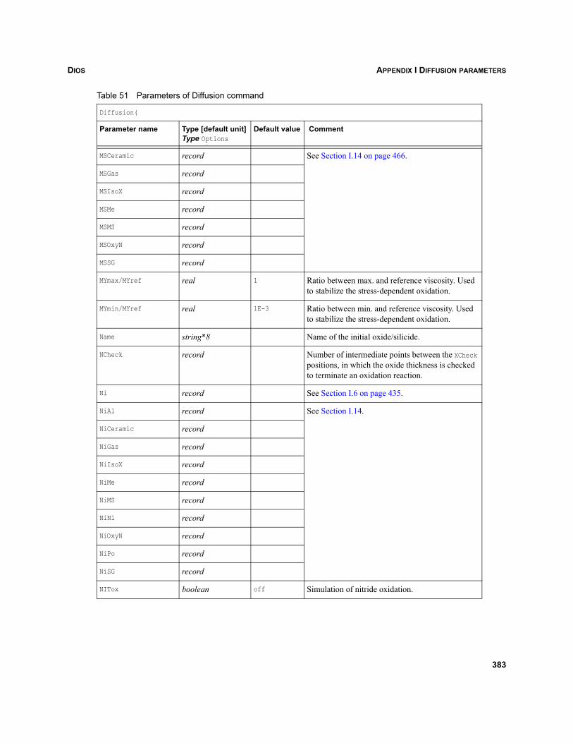
DIOS APPENDIX I DIFFUSION PARAMETERS
MSCeramic record See Section I.14 on page 466.
MSGas record
MSIsoX record
MSMe record
MSMS record
MSOxyN record
MSSG record
MYmax/MYref real 1 Ratio between max. and reference viscosity. Used to stabilize the stress-dependent oxidation.
MYmin/MYref real 1E-3 Ratio between min. and reference viscosity. Used to stabilize the stress-dependent oxidation.
Name string*8 Name of the initial oxide/silicide.
NCheck record Number of intermediate points between the XCheck positions, in which the oxide thickness is checked to terminate an oxidation reaction.
Ni record See Section I.6 on page 435.
NiAl record See Section I.14.
NiCeramic record
NiGas record
NiIsoX record
NiMe record
NiMS record
NiNi record
NiOxyN record
NiPo record
NiSG record
NITox boolean off Simulation of nitride oxidation.
Table 51 Parameters of Diffusion command
Diffusion(
Parameter name Type [default unit]Type Options
Default value Comment
383
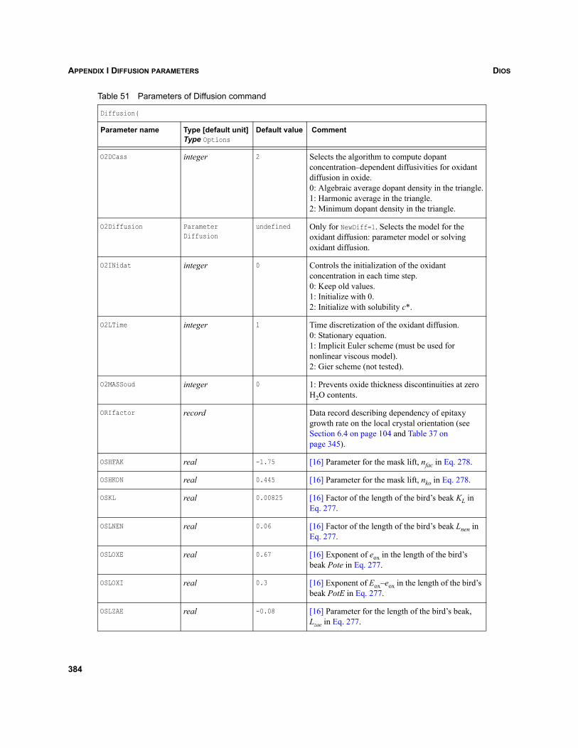
DIOSAPPENDIX I DIFFUSION PARAMETERS
O2DCass integer 2 Selects the algorithm to compute dopant concentration–dependent diffusivities for oxidant diffusion in oxide.0: Algebraic average dopant density in the triangle.1: Harmonic average in the triangle.2: Minimum dopant density in the triangle.
O2Diffusion ParameterDiffusion
undefined Only for NewDiff=1. Selects the model for the oxidant diffusion: parameter model or solving oxidant diffusion.
O2INidat integer 0 Controls the initialization of the oxidant concentration in each time step.0: Keep old values.1: Initialize with 0.2: Initialize with solubility c*.
O2LTime integer 1 Time discretization of the oxidant diffusion.0: Stationary equation.1: Implicit Euler scheme (must be used for nonlinear viscous model).2: Gier scheme (not tested).
O2MASSoud integer 0 1: Prevents oxide thickness discontinuities at zero H2O contents.
ORIfactor record Data record describing dependency of epitaxy growth rate on the local crystal orientation (see Section 6.4 on page 104 and Table 37 on page 345).
OSHFAK real -1.75 [16] Parameter for the mask lift, nfac in Eq. 278.
OSHKON real 0.445 [16] Parameter for the mask lift, nko in Eq. 278.
OSKL real 0.00825 [16] Factor of the length of the bird’s beak KL in Eq. 277.
OSLNEN real 0.06 [16] Factor of the length of the bird’s beak Lnen in Eq. 277.
OSLOXE real 0.67 [16] Exponent of eox in the length of the bird’s beak Pote in Eq. 277.
OSLOXI real 0.3 [16] Exponent of Eox–eox in the length of the bird’s beak PotE in Eq. 277.
OSLZAE real -0.08 [16] Parameter for the length of the bird’s beak, Lzae in Eq. 277.
Table 51 Parameters of Diffusion command
Diffusion(
Parameter name Type [default unit]Type Options
Default value Comment
384
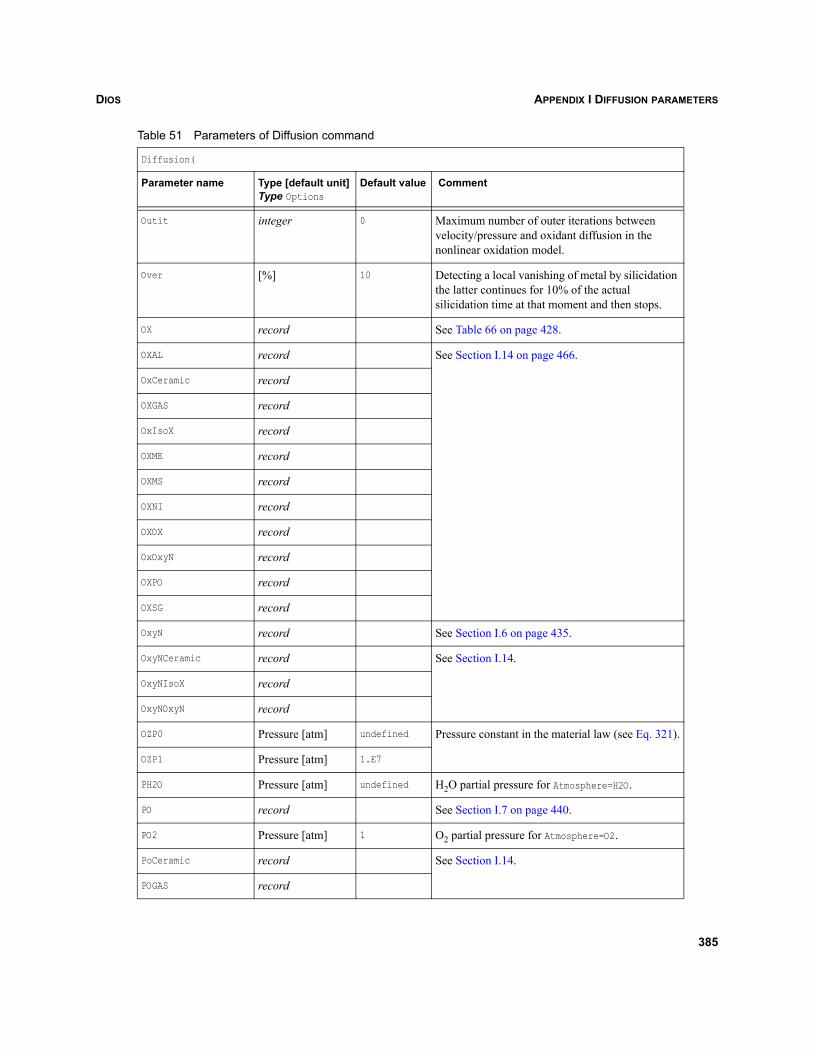
DIOS APPENDIX I DIFFUSION PARAMETERS
Outit integer 0 Maximum number of outer iterations between velocity/pressure and oxidant diffusion in the nonlinear oxidation model.
Over [%] 10 Detecting a local vanishing of metal by silicidation the latter continues for 10% of the actual silicidation time at that moment and then stops.
OX record See Table 66 on page 428.
OXAL record See Section I.14 on page 466.
OxCeramic record
OXGAS record
OxIsoX record
OXME record
OXMS record
OXNI record
OXOX record
OxOxyN record
OXPO record
OXSG record
OxyN record See Section I.6 on page 435.
OxyNCeramic record See Section I.14.
OxyNIsoX record
OxyNOxyN record
OZP0 Pressure [atm] undefined Pressure constant in the material law (see Eq. 321).
OZP1 Pressure [atm] 1.E7
PH2O Pressure [atm] undefined H2O partial pressure for Atmosphere=H2O.
PO record See Section I.7 on page 440.
PO2 Pressure [atm] 1 O2 partial pressure for Atmosphere=O2.
PoCeramic record See Section I.14.
POGAS record
Table 51 Parameters of Diffusion command
Diffusion(
Parameter name Type [default unit]Type Options
Default value Comment
385
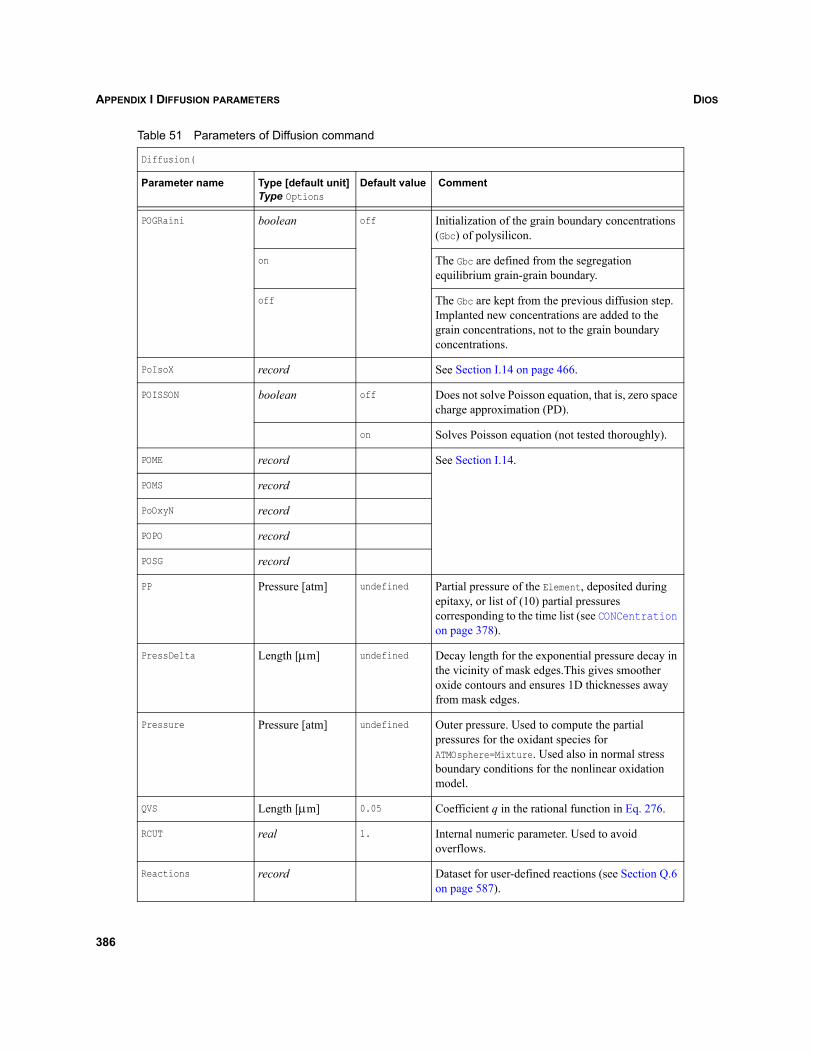
DIOSAPPENDIX I DIFFUSION PARAMETERS
POGRaini boolean off Initialization of the grain boundary concentrations (Gbc) of polysilicon.
on The Gbc are defined from the segregation equilibrium grain-grain boundary.
off The Gbc are kept from the previous diffusion step. Implanted new concentrations are added to the grain concentrations, not to the grain boundary concentrations.
PoIsoX record See Section I.14 on page 466.
POISSON boolean off Does not solve Poisson equation, that is, zero space charge approximation (PD).
on Solves Poisson equation (not tested thoroughly).
POME record See Section I.14.
POMS record
PoOxyN record
POPO record
POSG record
PP Pressure [atm] undefined Partial pressure of the Element, deposited during epitaxy, or list of (10) partial pressures corresponding to the time list (see CONCentration on page 378).
PressDelta Length [μm] undefined Decay length for the exponential pressure decay in the vicinity of mask edges.This gives smoother oxide contours and ensures 1D thicknesses away from mask edges.
Pressure Pressure [atm] undefined Outer pressure. Used to compute the partial pressures for the oxidant species for ATMOsphere=Mixture. Used also in normal stress boundary conditions for the nonlinear oxidation model.
QVS Length [μm] 0.05 Coefficient q in the rational function in Eq. 276.
RCUT real 1. Internal numeric parameter. Used to avoid overflows.
Reactions record Dataset for user-defined reactions (see Section Q.6 on page 587).
Table 51 Parameters of Diffusion command
Diffusion(
Parameter name Type [default unit]Type Options
Default value Comment
386
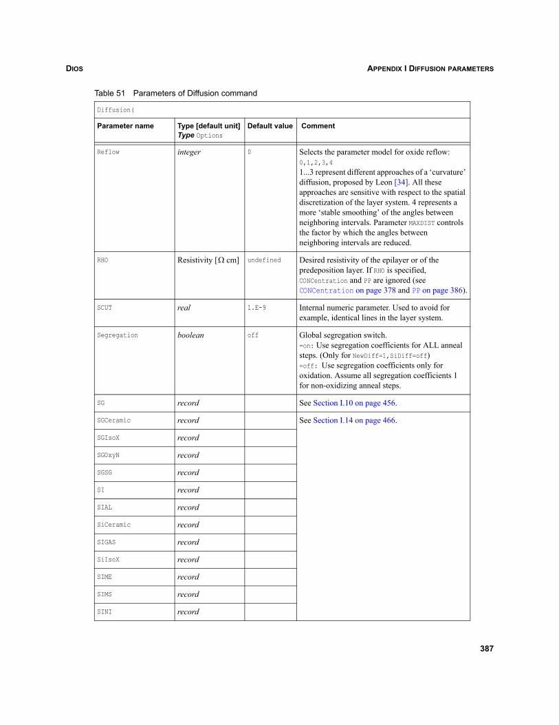
DIOS APPENDIX I DIFFUSION PARAMETERS
Reflow integer 0 Selects the parameter model for oxide reflow: 0,1,2,3,41...3 represent different approaches of a ‘curvature’ diffusion, proposed by Leon [34]. All these approaches are sensitive with respect to the spatial discretization of the layer system. 4 represents a more ‘stable smoothing’ of the angles between neighboring intervals. Parameter MAXDIST controls the factor by which the angles between neighboring intervals are reduced.
RHO Resistivity [ cm] undefined Desired resistivity of the epilayer or of the predeposition layer. If RHO is specified, CONCentration and PP are ignored (see CONCentration on page 378 and PP on page 386).
SCUT real 1.E-9 Internal numeric parameter. Used to avoid for example, identical lines in the layer system.
Segregation boolean off Global segregation switch.=on: Use segregation coefficients for ALL anneal steps. (Only for NewDiff=1,SiDiff=off)=off: Use segregation coefficients only for oxidation. Assume all segregation coefficients 1 for non-oxidizing anneal steps.
SG record See Section I.10 on page 456.
SGCeramic record See Section I.14 on page 466.
SGIsoX record
SGOxyN record
SGSG record
SI record
SIAL record
SiCeramic record
SIGAS record
SiIsoX record
SIME record
SIMS record
SINI record
Table 51 Parameters of Diffusion command
Diffusion(
Parameter name Type [default unit]Type Options
Default value Comment
Ω
387
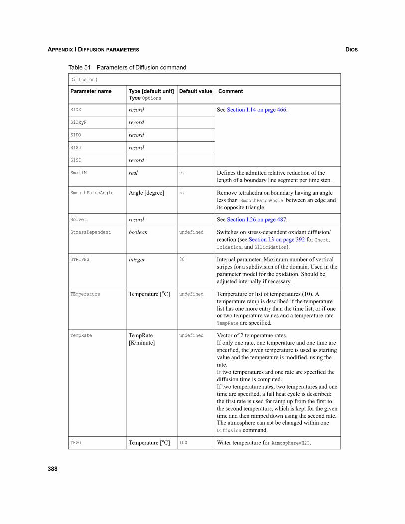
DIOSAPPENDIX I DIFFUSION PARAMETERS
SIOX record See Section I.14 on page 466.
SiOxyN record
SIPO record
SISG record
SISI record
SmallM real 0. Defines the admitted relative reduction of the length of a boundary line segment per time step.
SmoothPatchAngle Angle [degree] 5. Remove tetrahedra on boundary having an angle less than SmoothPatchAngle between an edge and its opposite triangle.
Solver record See Section I.26 on page 487.
StressDependent boolean undefined Switches on stress-dependent oxidant diffusion/reaction (see Section I.3 on page 392 for Inert, Oxidation, and Silicidation).
STRIPES integer 80 Internal parameter. Maximum number of vertical stripes for a subdivision of the domain. Used in the parameter model for the oxidation. Should be adjusted internally if necessary.
TEmperature Temperature [oC] undefined Temperature or list of temperatures (10). A temperature ramp is described if the temperature list has one more entry than the time list, or if one or two temperature values and a temperature rate TempRate are specified.
TempRate TempRate [K/minute]
undefined Vector of 2 temperature rates.If only one rate, one temperature and one time are specified, the given temperature is used as starting value and the temperature is modified, using the rate. If two temperatures and one rate are specified the diffusion time is computed.If two temperature rates, two temperatures and one time are specified, a full heat cycle is described: the first rate is used for ramp up from the first to the second temperature, which is kept for the given time and then ramped down using the second rate. The atmosphere can not be changed within one Diffusion command.
TH2O Temperature [oC] 100 Water temperature for Atmosphere=H2O.
Table 51 Parameters of Diffusion command
Diffusion(
Parameter name Type [default unit]Type Options
Default value Comment
388
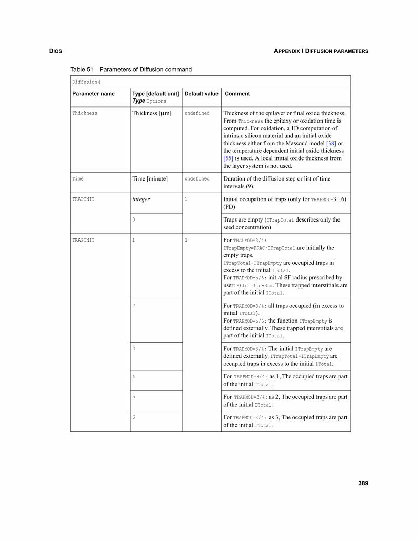
DIOS APPENDIX I DIFFUSION PARAMETERS
Thickness Thickness [μm] undefined Thickness of the epilayer or final oxide thickness. From Thickness the epitaxy or oxidation time is computed. For oxidation, a 1D computation of intrinsic silicon material and an initial oxide thickness either from the Massoud model [38] or the temperature dependent initial oxide thickness [55] is used. A local initial oxide thickness from the layer system is not used.
Time Time [minute] undefined Duration of the diffusion step or list of time intervals (9).
TRAPINIT integer 1 Initial occupation of traps (only for TRAPMOD=3...6) (PD)
0 Traps are empty (ITrapTotal describes only the seed concentration)
TRAPINIT 1 1 For TRAPMOD=3/4:ITrapEmpty=FRAC·ITrapTotal are initially the empty traps.ITrapTotal-ITrapEmpty are occupied traps in excess to the initial ITotal.For TRAPMOD=5/6: initial SF radius prescribed by user: SFIni=1.d-3nm. These trapped interstitials are part of the initial ITotal.
2 For TRAPMOD=3/4: all traps occupied (in excess to initial ITotal).For TRAPMOD=5/6: the function ITrapEmpty is defined externally. These trapped interstitials are part of the initial ITotal.
3 For TRAPMOD=3/4: The initial ITrapEmpty are defined externally. ITrapTotal-ITrapEmpty are occupied traps in excess to the initial ITotal.
4 For TRAPMOD=3/4: as 1, The occupied traps are part of the initial ITotal.
5 For TRAPMOD=3/4: as 2, The occupied traps are part of the initial ITotal.
6 For TRAPMOD=3/4: as 3, The occupied traps are part of the initial ITotal.
Table 51 Parameters of Diffusion command
Diffusion(
Parameter name Type [default unit]Type Options
Default value Comment
389
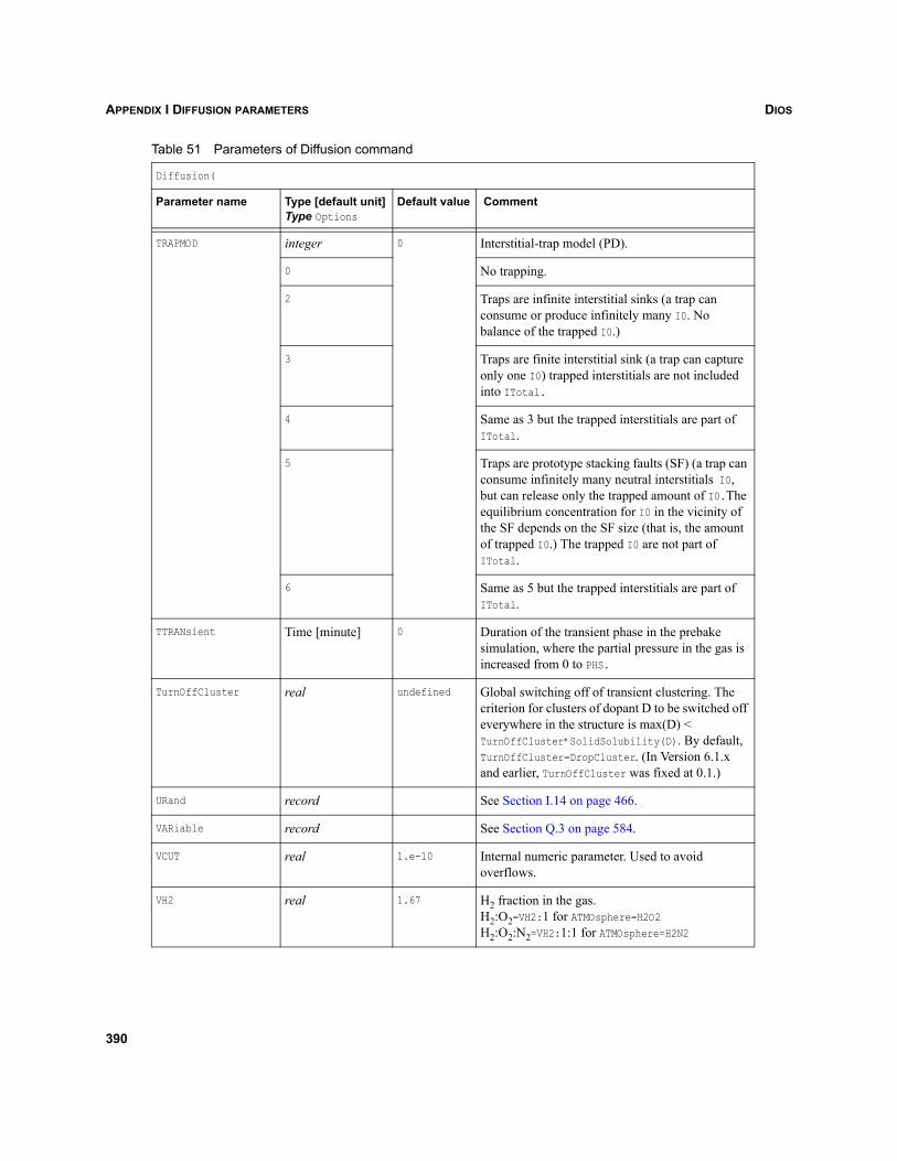
DIOSAPPENDIX I DIFFUSION PARAMETERS
TRAPMOD integer 0 Interstitial-trap model (PD).
0 No trapping.
2 Traps are infinite interstitial sinks (a trap can consume or produce infinitely many I0. No balance of the trapped I0.)
3 Traps are finite interstitial sink (a trap can capture only one I0) trapped interstitials are not included into ITotal.
4 Same as 3 but the trapped interstitials are part of ITotal.
5 Traps are prototype stacking faults (SF) (a trap can consume infinitely many neutral interstitials I0, but can release only the trapped amount of I0.The equilibrium concentration for I0 in the vicinity of the SF depends on the SF size (that is, the amount of trapped I0.) The trapped I0 are not part of ITotal.
6 Same as 5 but the trapped interstitials are part of ITotal.
TTRANsient Time [minute] 0 Duration of the transient phase in the prebake simulation, where the partial pressure in the gas is increased from 0 to PHS.
TurnOffCluster real undefined Global switching off of transient clustering. The criterion for clusters of dopant D to be switched off everywhere in the structure is max(D) < TurnOffCluster*SolidSolubility(D). By default, TurnOffCluster=DropCluster. (In Version 6.1.x and earlier, TurnOffCluster was fixed at 0.1.)
URand record See Section I.14 on page 466.
VARiable record See Section Q.3 on page 584.
VCUT real 1.e-10 Internal numeric parameter. Used to avoid overflows.
VH2 real 1.67 H2 fraction in the gas.H2:O2=VH2:1 for ATMOsphere=H2O2H2:O2:N2=VH2:1:1 for ATMOsphere=H2N2
Table 51 Parameters of Diffusion command
Diffusion(
Parameter name Type [default unit]Type Options
Default value Comment
390
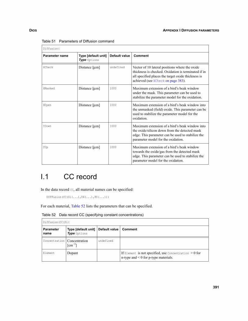
DIOS APPENDIX I DIFFUSION PARAMETERS
I.1 CC recordIn the data record CC, all material names can be specified:
DIFFusion(CC(Si(...),OX(...),PO(...)))
For each material, Table 52 lists the parameters that can be specified.
XCheck Distance [μm] undefined Vector of 10 lateral positions where the oxide thickness is checked. Oxidation is terminated if in all specified places the target oxide thickness is achieved (see NCheck on page 383).
XMasked Distance [μm] 1000 Maximum extension of a bird’s beak window under the mask. This parameter can be used to stabilize the parameter model for the oxidation.
XOpen Distance [μm] 1000 Maximum extension of a bird’s beak window into the unmasked (field) oxide. This parameter can be used to stabilize the parameter model for the oxidation.
YDown Distance [μm] 1000 Maximum extension of a bird’s beak window into the oxide/silicon down from the detected mask edge. This parameter can be used to stabilize the parameter model for the oxidation.
YUp Distance [μm] 1000 Maximum extension of a bird’s beak window towards the oxide/gas from the detected mask edge. This parameter can be used to stabilize the parameter model for the oxidation.
Table 52 Data record CC (specifying constant concentrations)
Diffusion(CC(Si(
Parameter name
Type [default unit]Type Options
Default value Comment
Concentration Concentration [cm–3]
undefined
Element Dopant If Element is not specified, use Concentration > 0 for n-type and < 0 for p-type materials.
Table 51 Parameters of Diffusion command
Diffusion(
Parameter name Type [default unit]Type Options
Default value Comment
391
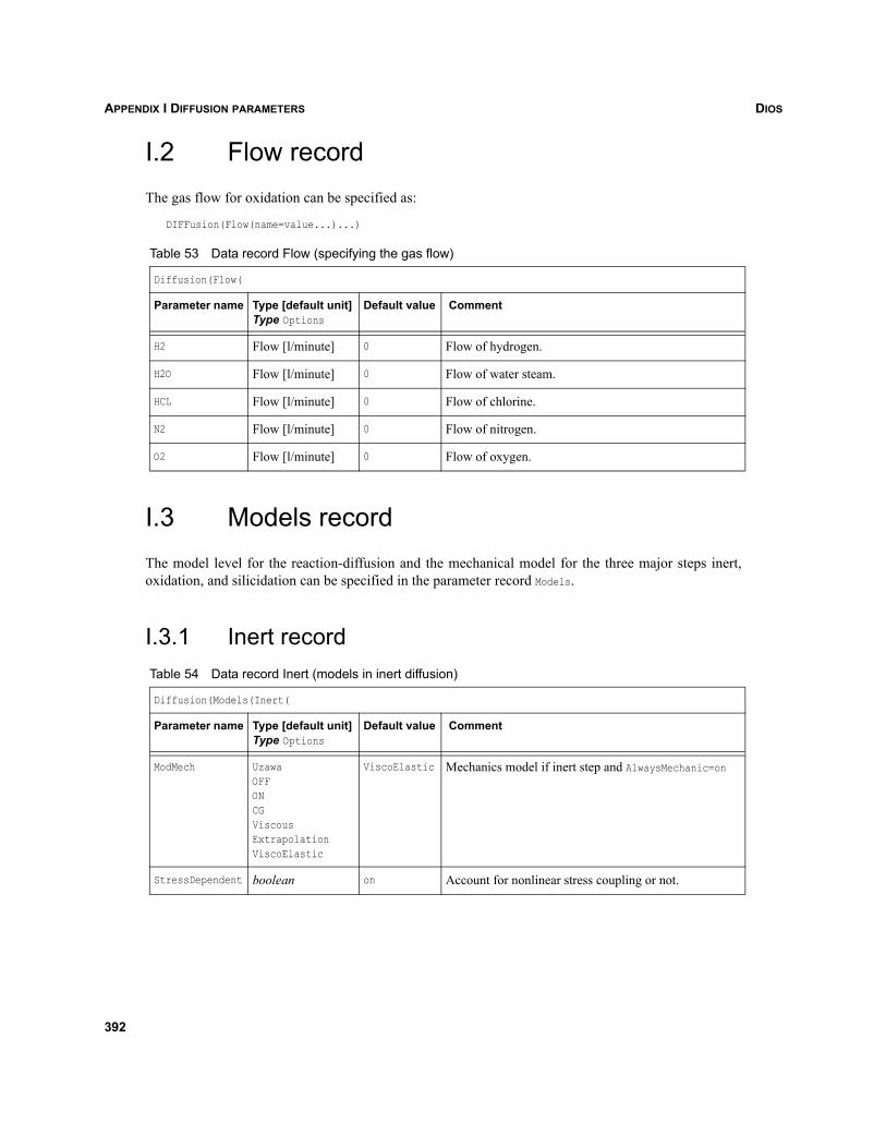
DIOSAPPENDIX I DIFFUSION PARAMETERS
I.2 Flow recordThe gas flow for oxidation can be specified as:
DIFFusion(Flow(name=value...)...)
I.3 Models recordThe model level for the reaction-diffusion and the mechanical model for the three major steps inert,oxidation, and silicidation can be specified in the parameter record Models.
I.3.1 Inert record
Table 53 Data record Flow (specifying the gas flow)
Diffusion(Flow(
Parameter name Type [default unit]Type Options
Default value Comment
H2 Flow [l/minute] 0 Flow of hydrogen.
H2O Flow [l/minute] 0 Flow of water steam.
HCL Flow [l/minute] 0 Flow of chlorine.
N2 Flow [l/minute] 0 Flow of nitrogen.
O2 Flow [l/minute] 0 Flow of oxygen.
Table 54 Data record Inert (models in inert diffusion)
Diffusion(Models(Inert(
Parameter name Type [default unit]Type Options
Default value Comment
ModMech UzawaOFF ON CG Viscous Extrapolation ViscoElastic
ViscoElastic Mechanics model if inert step and AlwaysMechanic=on
StressDependent boolean on Account for nonlinear stress coupling or not.
392
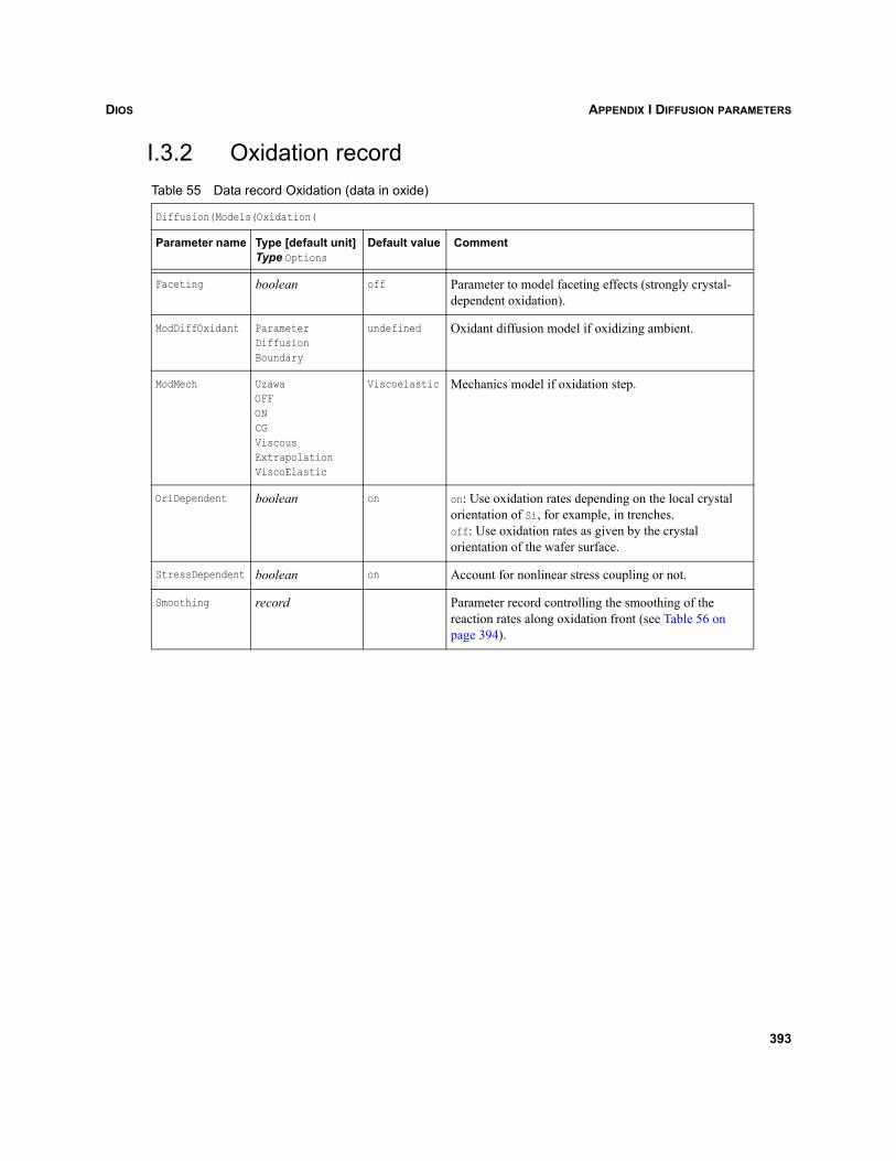
DIOS APPENDIX I DIFFUSION PARAMETERS
I.3.2 Oxidation recordTable 55 Data record Oxidation (data in oxide)
Diffusion(Models(Oxidation(
Parameter name Type [default unit]Type Options
Default value Comment
Faceting boolean off Parameter to model faceting effects (strongly crystal-dependent oxidation).
ModDiffOxidant Parameter Diffusion Boundary
undefined Oxidant diffusion model if oxidizing ambient.
ModMech UzawaOFFON CG Viscous Extrapolation ViscoElastic
Viscoelastic Mechanics model if oxidation step.
OriDependent boolean on on: Use oxidation rates depending on the local crystal orientation of Si, for example, in trenches.off: Use oxidation rates as given by the crystal orientation of the wafer surface.
StressDependent boolean on Account for nonlinear stress coupling or not.
Smoothing record Parameter record controlling the smoothing of the reaction rates along oxidation front (see Table 56 on page 394).
393
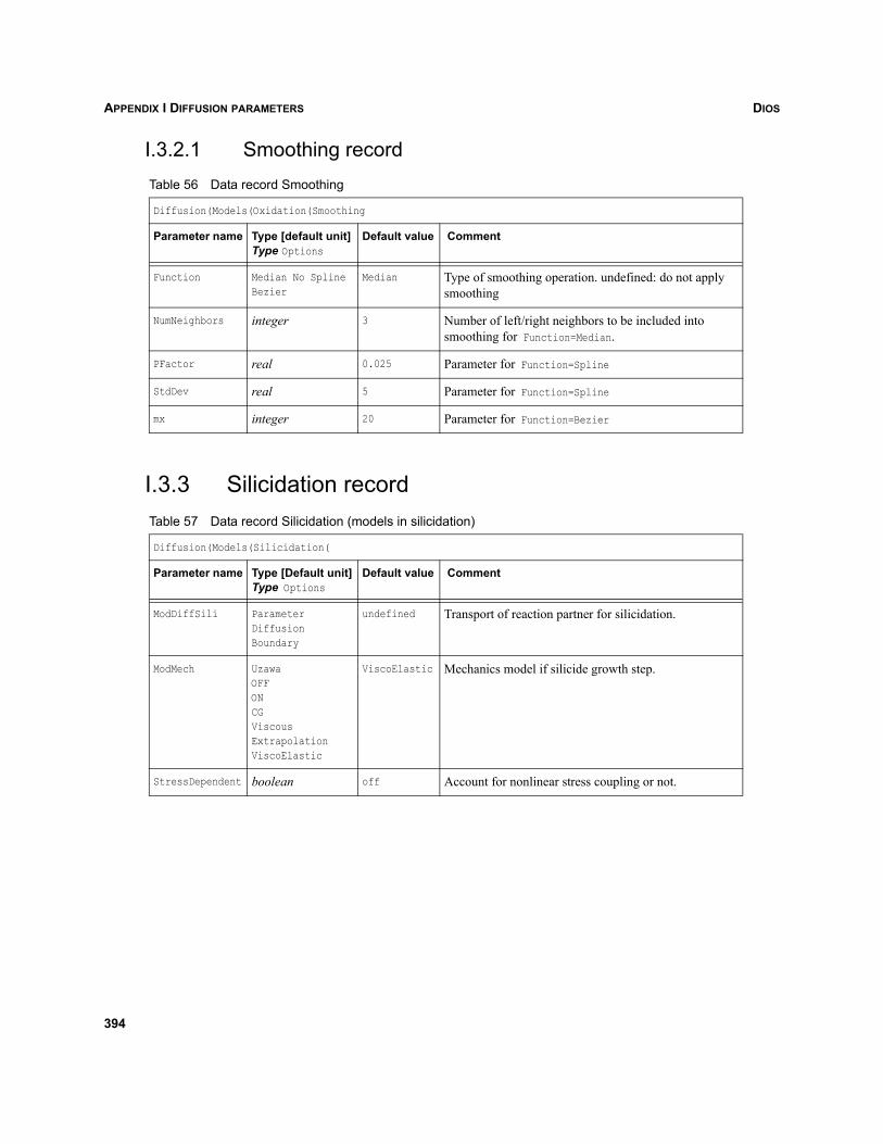
DIOSAPPENDIX I DIFFUSION PARAMETERS
I.3.2.1 Smoothing record
I.3.3 Silicidation record
Table 56 Data record Smoothing
Diffusion(Models(Oxidation(Smoothing
Parameter name Type [default unit]Type Options
Default value Comment
Function Median No Spline Bezier
Median Type of smoothing operation. undefined: do not apply smoothing
NumNeighbors integer 3 Number of left/right neighbors to be included into smoothing for Function=Median.
PFactor real 0.025 Parameter for Function=Spline
StdDev real 5 Parameter for Function=Spline
mx integer 20 Parameter for Function=Bezier
Table 57 Data record Silicidation (models in silicidation)
Diffusion(Models(Silicidation(
Parameter name Type [Default unit]Type Options
Default value Comment
ModDiffSili ParameterDiffusion Boundary
undefined Transport of reaction partner for silicidation.
ModMech UzawaOFFON CGViscousExtrapolation ViscoElastic
ViscoElastic Mechanics model if silicide growth step.
StressDependent boolean off Account for nonlinear stress coupling or not.
394
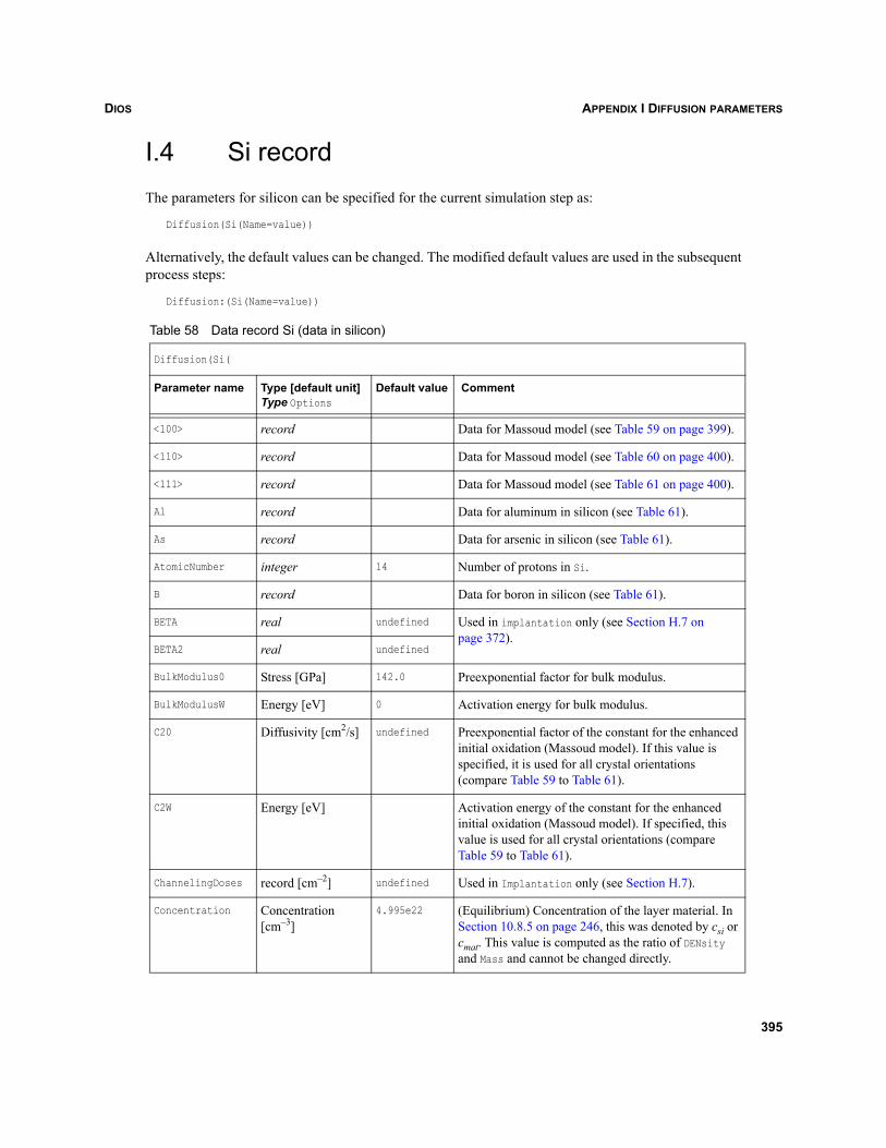
DIOS APPENDIX I DIFFUSION PARAMETERS
I.4 Si recordThe parameters for silicon can be specified for the current simulation step as:
Diffusion(Si(Name=value))
Alternatively, the default values can be changed. The modified default values are used in the subsequentprocess steps:
Diffusion:(Si(Name=value))
Table 58 Data record Si (data in silicon)
Diffusion(Si(
Parameter name Type [default unit]Type Options
Default value Comment
<100> record Data for Massoud model (see Table 59 on page 399).
<110> record Data for Massoud model (see Table 60 on page 400).
<111> record Data for Massoud model (see Table 61 on page 400).
Al record Data for aluminum in silicon (see Table 61).
As record Data for arsenic in silicon (see Table 61).
AtomicNumber integer 14 Number of protons in Si.
B record Data for boron in silicon (see Table 61).
BETA real undefined Used in implantation only (see Section H.7 on page 372).
BETA2 real undefined
BulkModulus0 Stress [GPa] 142.0 Preexponential factor for bulk modulus.
BulkModulusW Energy [eV] 0 Activation energy for bulk modulus.
C20 Diffusivity [cm2/s] undefined Preexponential factor of the constant for the enhanced initial oxidation (Massoud model). If this value is specified, it is used for all crystal orientations (compare Table 59 to Table 61).
C2W Energy [eV] Activation energy of the constant for the enhanced initial oxidation (Massoud model). If specified, this value is used for all crystal orientations (compare Table 59 to Table 61).
ChannelingDoses record [cm–2] undefined Used in Implantation only (see Section H.7).
Concentration Concentration [cm–3]
4.995e22 (Equilibrium) Concentration of the layer material. In Section 10.8.5 on page 246, this was denoted by csi or cmat. This value is computed as the ratio of DENsity and Mass and cannot be changed directly.
395
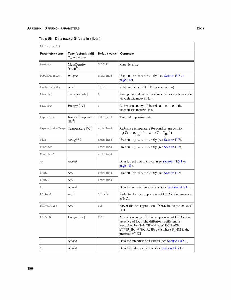
DIOSAPPENDIX I DIFFUSION PARAMETERS
Density MassDensity[g/cm3]
2.33221 Mass density.
DepthDependent integer undefined Used in Implantation only (see Section H.7 on page 372).
Dielectricity real 11.67 Relative dielectricity (Poisson equation).
Elastic0 Time [minute] 0 Preexponential factor for elastic relaxation time in the viscoelastic material law.
ElasticW Energy [eV] 0 Activation energy of the relaxation time in the viscoelastic material law.
Expansion InverseTemperature [K–1]
1.0579e-0 Thermal expansion rate.
ExpansionRefTemp Temperature [oC] undefined Reference temperature for equilibrium density
File string*80 undefined Used in Implantation only (see Section H.7).
Function undefined Used in Implantation only (see Section H.7).
Function2 undefined
Ga record Data for gallium in silicon (see Section I.4.5.1 on page 411).
GAMma real undefined Used in Implantation only (see Section H.7).
GAMma2 real undefined
Ge record Data for germanium in silicon (see Section I.4.5.1).
HClRed0 real 2.31e34 Prefactor for the suppression of OED in the presence of HCl.
HClRedPower real 0.5 Power for the suppression of OED in the presence of HCl.
HClRedW Energy [eV] 8.88 Activation energy for the suppression of OED in the presence of HCl. The diffusion coefficient is multiplied by (1+HClRed0*exp(-HClRedW/kT)*(P_HCl)**HClRedPower) where P_HCl is the pressure of HCl.
I record Data for interstitials in silicon (see Section I.4.5.1).
In record Data for indium in silicon (see Section I.4.5.1).
Table 58 Data record Si (data in silicon)
Diffusion(Si(
Parameter name Type [default unit]Type Options
Default value Comment
ρ0 T( ) ρ0REF1 a1 T TREF–( )⋅–( )⋅=
396
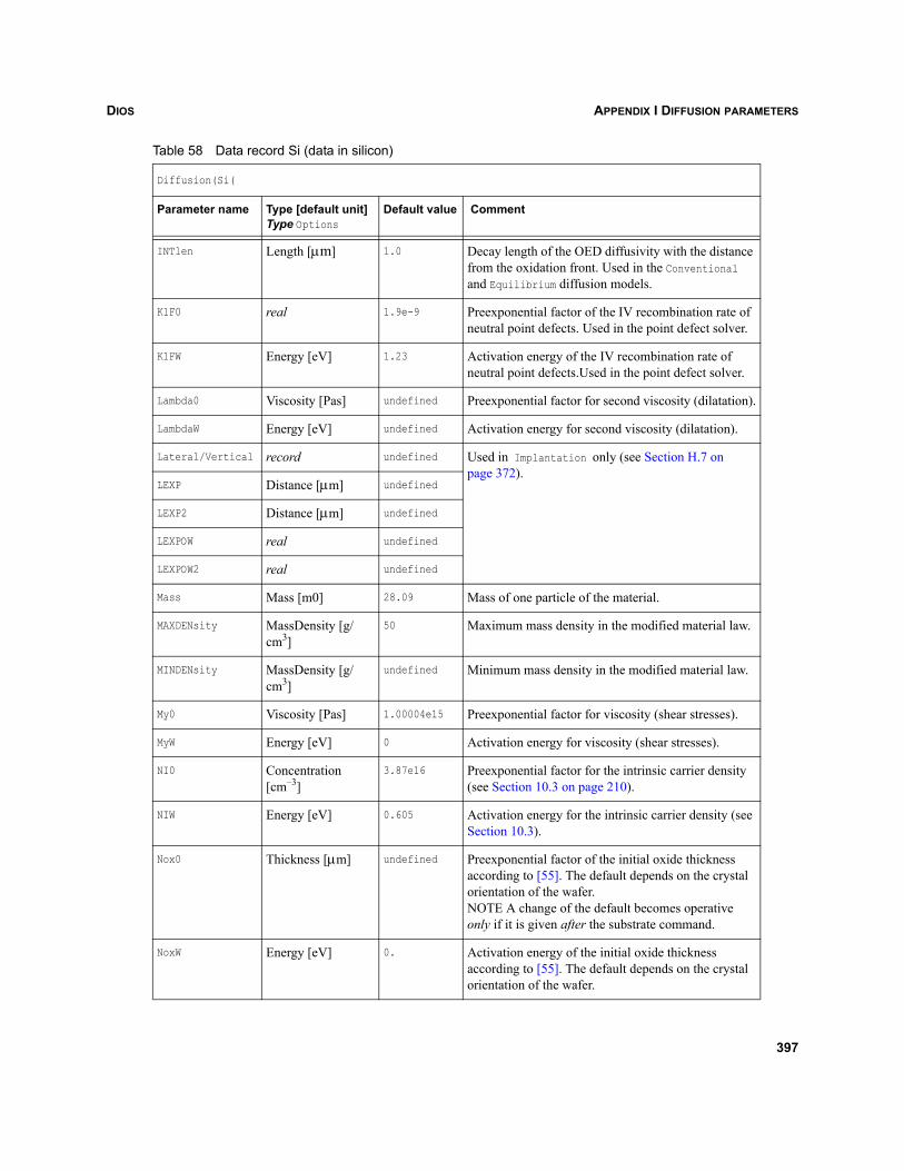
DIOS APPENDIX I DIFFUSION PARAMETERS
INTlen Length [μm] 1.0 Decay length of the OED diffusivity with the distance from the oxidation front. Used in the Conventional and Equilibrium diffusion models.
K1F0 real 1.9e-9 Preexponential factor of the IV recombination rate of neutral point defects. Used in the point defect solver.
K1FW Energy [eV] 1.23 Activation energy of the IV recombination rate of neutral point defects.Used in the point defect solver.
Lambda0 Viscosity [Pas] undefined Preexponential factor for second viscosity (dilatation).
LambdaW Energy [eV] undefined Activation energy for second viscosity (dilatation).
Lateral/Vertical record undefined Used in Implantation only (see Section H.7 on page 372).
LEXP Distance [μm] undefined
LEXP2 Distance [μm] undefined
LEXPOW real undefined
LEXPOW2 real undefined
Mass Mass [m0] 28.09 Mass of one particle of the material.
MAXDENsity MassDensity [g/cm3]
50 Maximum mass density in the modified material law.
MINDENsity MassDensity [g/cm3]
undefined Minimum mass density in the modified material law.
My0 Viscosity [Pas] 1.00004e15 Preexponential factor for viscosity (shear stresses).
MyW Energy [eV] 0 Activation energy for viscosity (shear stresses).
NI0 Concentration [cm–3]
3.87e16 Preexponential factor for the intrinsic carrier density (see Section 10.3 on page 210).
NIW Energy [eV] 0.605 Activation energy for the intrinsic carrier density (see Section 10.3).
Nox0 Thickness [μm] undefined Preexponential factor of the initial oxide thickness according to [55]. The default depends on the crystal orientation of the wafer.NOTE A change of the default becomes operative only if it is given after the substrate command.
NoxW Energy [eV] 0. Activation energy of the initial oxide thickness according to [55]. The default depends on the crystal orientation of the wafer.
Table 58 Data record Si (data in silicon)
Diffusion(Si(
Parameter name Type [default unit]Type Options
Default value Comment
397
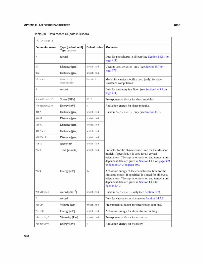
DIOSAPPENDIX I DIFFUSION PARAMETERS
P record Data for phosphorus in silicon (see Section I.4.5.1 on page 411).
RP Distance [μm] undefined Used in Implantation only (see Section H.7 on page 372).
RP2 Distance [μm] undefined
RSmodel Masetti | Antoniadis
Masetti Model for carrier mobility used (only) for sheet resistance computation.
Sb record Data for antimony in silicon (see Section I.4.5.1 on page 411).
ShearModulus0 Stress [GPa] 73.0 Preexponential factor for shear modulus.
ShearModulusW Energy [eV] 0 Activation energy for shear modulus.
STDV Distance [μm] undefined Used in Implantation only (see Section H.7).
STDV2 Distance [μm] undefined
STDVL Distance [μm] undefined
STDVSec Distance [μm] undefined
STDVSec2 Distance [μm] undefined
Table string*80 undefined
Tau0 Time [minute] undefined Prefactor for the characteristic time for the Massoud model. If specified, it is used for all crystal orientations. The crystal orientation and temperature-dependent data are given in Section I.4.1 on page 399 to Section I.4.3 on page 400.
TauW Energy [eV] 0. Activation energy of the characteristic time for the Massoud model. If specified, it is used for all crystal orientations. The crystal orientation and temperature-dependent data are given in Section I.4.1 to Section I.4.3.
TotalDoses record [cm–2] undefined Used in Implantation only (see Section H.7).
V record Data for vacancies in silicon (see Section I.4.5.1).
Vcrit0 Volume [μm3] undefined Preexponential factor for shear stress coupling.
VcritW Energy [eV] undefined Activation energy for shear stress coupling.
Viscosity0 Viscosity [Pas] undefined Preexponential factor for viscosity.
ViscosityW Energy [eV] 0 Activation energy for viscosity.
Table 58 Data record Si (data in silicon)
Diffusion(Si(
Parameter name Type [default unit]Type Options
Default value Comment
398
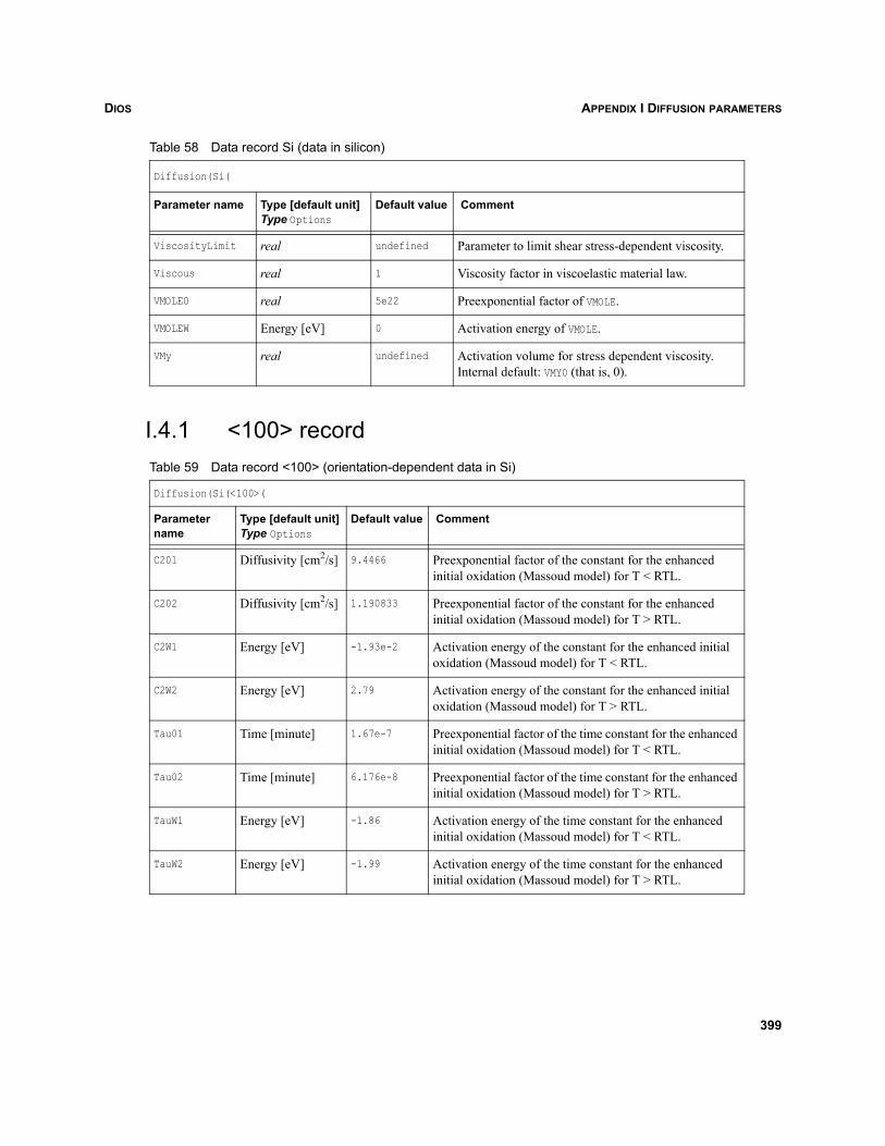
DIOS APPENDIX I DIFFUSION PARAMETERS
I.4.1 <100> record
ViscosityLimit real undefined Parameter to limit shear stress-dependent viscosity.
Viscous real 1 Viscosity factor in viscoelastic material law.
VMOLE0 real 5e22 Preexponential factor of VMOLE.
VMOLEW Energy [eV] 0 Activation energy of VMOLE.
VMy real undefined Activation volume for stress dependent viscosity. Internal default: VMY0 (that is, 0).
Table 59 Data record <100> (orientation-dependent data in Si)
Diffusion(Si(<100>(
Parameter name
Type [default unit]Type Options
Default value Comment
C201 Diffusivity [cm2/s] 9.4466 Preexponential factor of the constant for the enhanced initial oxidation (Massoud model) for T < RTL.
C202 Diffusivity [cm2/s] 1.190833 Preexponential factor of the constant for the enhanced initial oxidation (Massoud model) for T > RTL.
C2W1 Energy [eV] -1.93e-2 Activation energy of the constant for the enhanced initial oxidation (Massoud model) for T < RTL.
C2W2 Energy [eV] 2.79 Activation energy of the constant for the enhanced initial oxidation (Massoud model) for T > RTL.
Tau01 Time [minute] 1.67e-7 Preexponential factor of the time constant for the enhanced initial oxidation (Massoud model) for T < RTL.
Tau02 Time [minute] 6.176e-8 Preexponential factor of the time constant for the enhanced initial oxidation (Massoud model) for T > RTL.
TauW1 Energy [eV] -1.86 Activation energy of the time constant for the enhanced initial oxidation (Massoud model) for T < RTL.
TauW2 Energy [eV] -1.99 Activation energy of the time constant for the enhanced initial oxidation (Massoud model) for T > RTL.
Table 58 Data record Si (data in silicon)
Diffusion(Si(
Parameter name Type [default unit]Type Options
Default value Comment
399
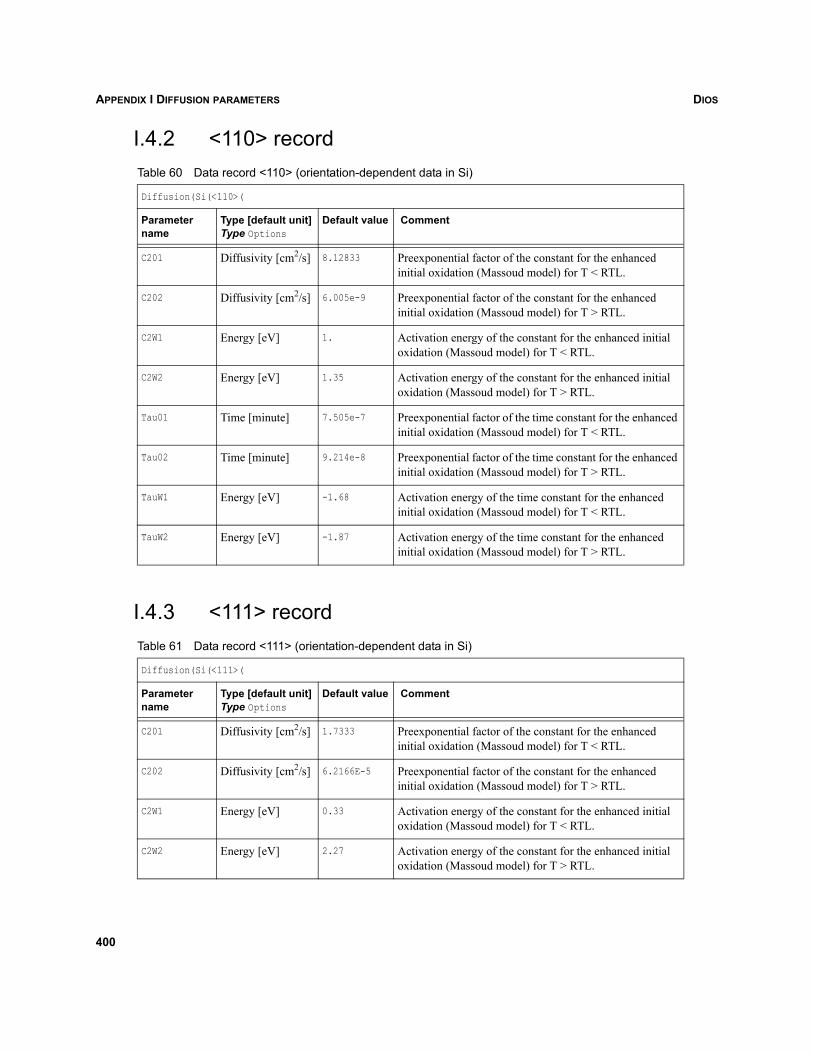
DIOSAPPENDIX I DIFFUSION PARAMETERS
I.4.2 <110> record
I.4.3 <111> record
Table 60 Data record <110> (orientation-dependent data in Si)
Diffusion(Si(<110>(
Parameter name
Type [default unit]Type Options
Default value Comment
C201 Diffusivity [cm2/s] 8.12833 Preexponential factor of the constant for the enhanced initial oxidation (Massoud model) for T < RTL.
C202 Diffusivity [cm2/s] 6.005e-9 Preexponential factor of the constant for the enhanced initial oxidation (Massoud model) for T > RTL.
C2W1 Energy [eV] 1. Activation energy of the constant for the enhanced initial oxidation (Massoud model) for T < RTL.
C2W2 Energy [eV] 1.35 Activation energy of the constant for the enhanced initial oxidation (Massoud model) for T > RTL.
Tau01 Time [minute] 7.505e-7 Preexponential factor of the time constant for the enhanced initial oxidation (Massoud model) for T < RTL.
Tau02 Time [minute] 9.214e-8 Preexponential factor of the time constant for the enhanced initial oxidation (Massoud model) for T > RTL.
TauW1 Energy [eV] -1.68 Activation energy of the time constant for the enhanced initial oxidation (Massoud model) for T < RTL.
TauW2 Energy [eV] -1.87 Activation energy of the time constant for the enhanced initial oxidation (Massoud model) for T > RTL.
Table 61 Data record <111> (orientation-dependent data in Si)
Diffusion(Si(<111>(
Parameter name
Type [default unit]Type Options
Default value Comment
C201 Diffusivity [cm2/s] 1.7333 Preexponential factor of the constant for the enhanced initial oxidation (Massoud model) for T < RTL.
C202 Diffusivity [cm2/s] 6.2166E-5 Preexponential factor of the constant for the enhanced initial oxidation (Massoud model) for T > RTL.
C2W1 Energy [eV] 0.33 Activation energy of the constant for the enhanced initial oxidation (Massoud model) for T < RTL.
C2W2 Energy [eV] 2.27 Activation energy of the constant for the enhanced initial oxidation (Massoud model) for T > RTL.
400
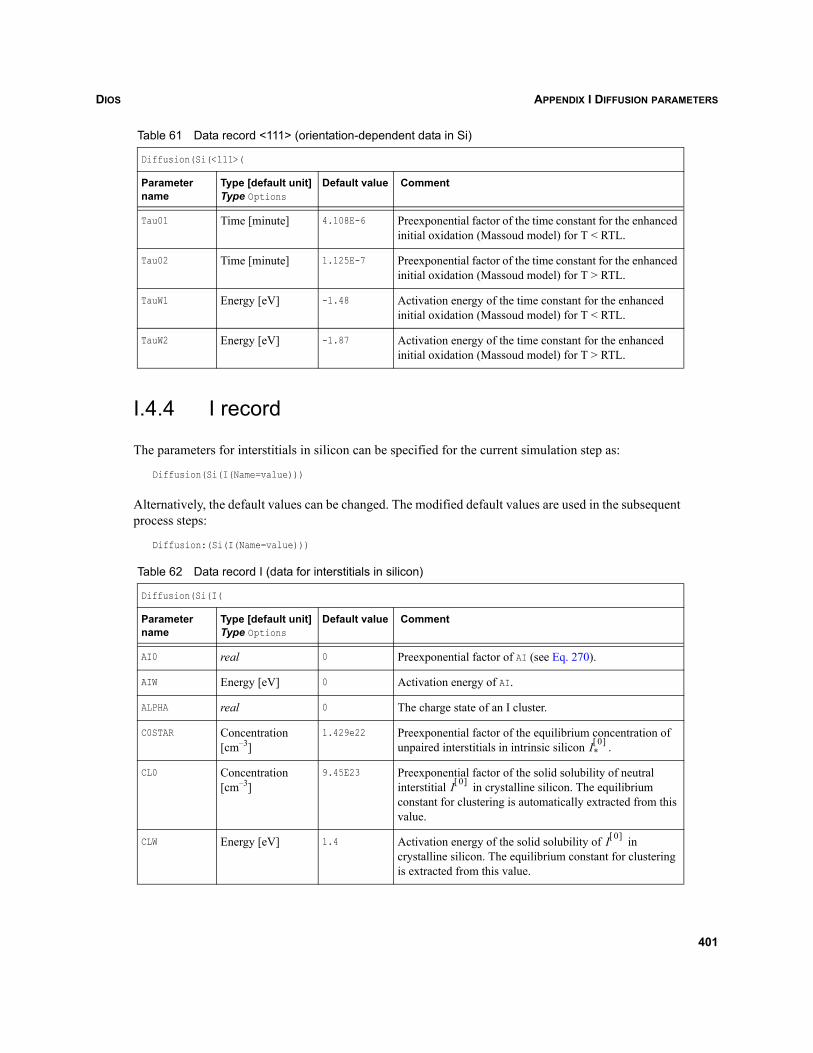
DIOS APPENDIX I DIFFUSION PARAMETERS
I.4.4 I record
The parameters for interstitials in silicon can be specified for the current simulation step as:
Diffusion(Si(I(Name=value)))
Alternatively, the default values can be changed. The modified default values are used in the subsequentprocess steps:
Diffusion:(Si(I(Name=value)))
Tau01 Time [minute] 4.108E-6 Preexponential factor of the time constant for the enhanced initial oxidation (Massoud model) for T < RTL.
Tau02 Time [minute] 1.125E-7 Preexponential factor of the time constant for the enhanced initial oxidation (Massoud model) for T > RTL.
TauW1 Energy [eV] -1.48 Activation energy of the time constant for the enhanced initial oxidation (Massoud model) for T < RTL.
TauW2 Energy [eV] -1.87 Activation energy of the time constant for the enhanced initial oxidation (Massoud model) for T > RTL.
Table 62 Data record I (data for interstitials in silicon)
Diffusion(Si(I(
Parameter name
Type [default unit]Type Options
Default value Comment
AI0 real 0 Preexponential factor of AI (see Eq. 270).
AIW Energy [eV] 0 Activation energy of AI.
ALPHA real 0 The charge state of an I cluster.
C0STAR Concentration [cm–3]
1.429e22 Preexponential factor of the equilibrium concentration of unpaired interstitials in intrinsic silicon .
CL0 Concentration [cm–3]
9.45E23 Preexponential factor of the solid solubility of neutral interstitial in crystalline silicon. The equilibrium constant for clustering is automatically extracted from this value.
CLW Energy [eV] 1.4 Activation energy of the solid solubility of in crystalline silicon. The equilibrium constant for clustering is extracted from this value.
Table 61 Data record <111> (orientation-dependent data in Si)
Diffusion(Si(<111>(
Parameter name
Type [default unit]Type Options
Default value Comment
I*0[ ]
I 0[ ]
I 0[ ]
401
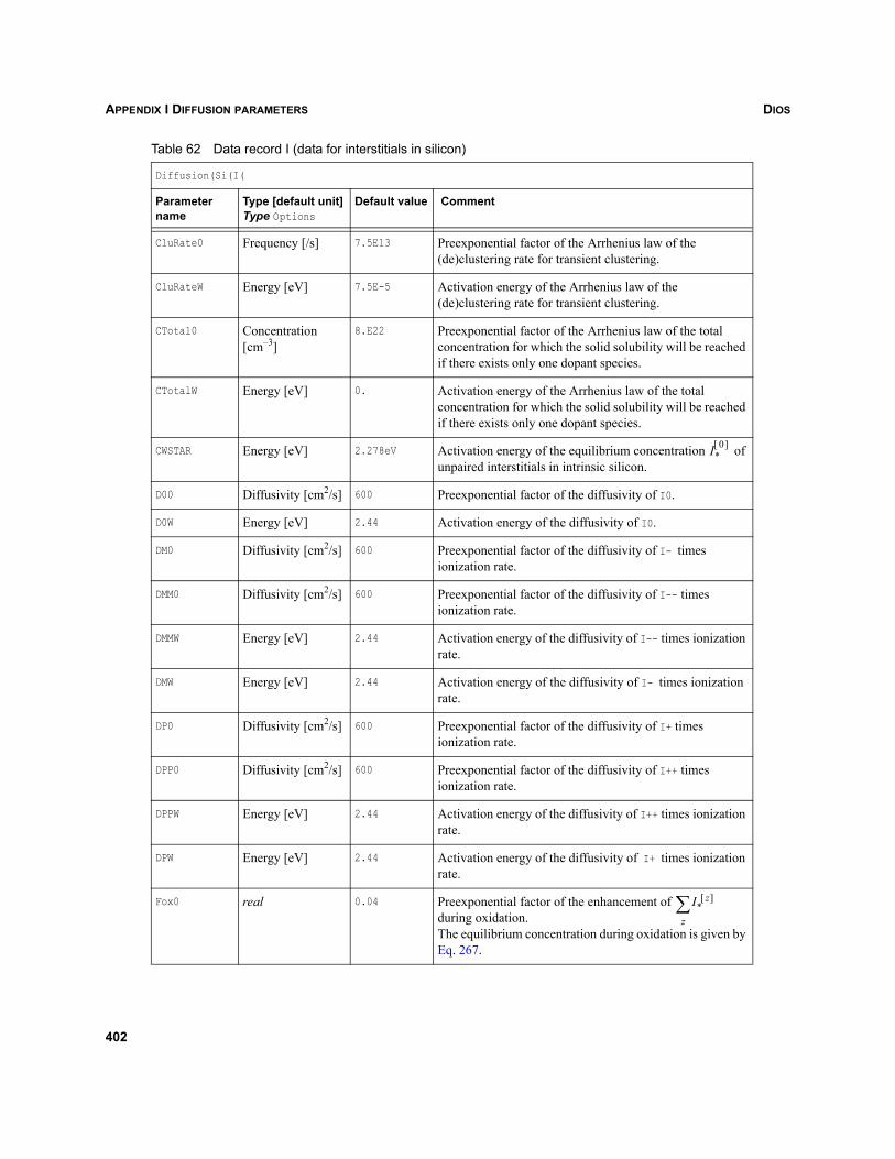
DIOSAPPENDIX I DIFFUSION PARAMETERS
CluRate0 Frequency [/s] 7.5E13 Preexponential factor of the Arrhenius law of the (de)clustering rate for transient clustering.
CluRateW Energy [eV] 7.5E-5 Activation energy of the Arrhenius law of the (de)clustering rate for transient clustering.
CTotal0 Concentration [cm–3]
8.E22 Preexponential factor of the Arrhenius law of the total concentration for which the solid solubility will be reached if there exists only one dopant species.
CTotalW Energy [eV] 0. Activation energy of the Arrhenius law of the total concentration for which the solid solubility will be reached if there exists only one dopant species.
CWSTAR Energy [eV] 2.278eV Activation energy of the equilibrium concentration of unpaired interstitials in intrinsic silicon.
D00 Diffusivity [cm2/s] 600 Preexponential factor of the diffusivity of I0.
D0W Energy [eV] 2.44 Activation energy of the diffusivity of I0.
DM0 Diffusivity [cm2/s] 600 Preexponential factor of the diffusivity of I- times ionization rate.
DMM0 Diffusivity [cm2/s] 600 Preexponential factor of the diffusivity of I-- times ionization rate.
DMMW Energy [eV] 2.44 Activation energy of the diffusivity of I-- times ionization rate.
DMW Energy [eV] 2.44 Activation energy of the diffusivity of I- times ionization rate.
DP0 Diffusivity [cm2/s] 600 Preexponential factor of the diffusivity of I+ times ionization rate.
DPP0 Diffusivity [cm2/s] 600 Preexponential factor of the diffusivity of I++ times ionization rate.
DPPW Energy [eV] 2.44 Activation energy of the diffusivity of I++ times ionization rate.
DPW Energy [eV] 2.44 Activation energy of the diffusivity of I+ times ionization rate.
Fox0 real 0.04 Preexponential factor of the enhancement of during oxidation. The equilibrium concentration during oxidation is given by Eq. 267.
Table 62 Data record I (data for interstitials in silicon)
Diffusion(Si(I(
Parameter name
Type [default unit]Type Options
Default value Comment
I*0[ ]
I*z[ ]
z∑
402
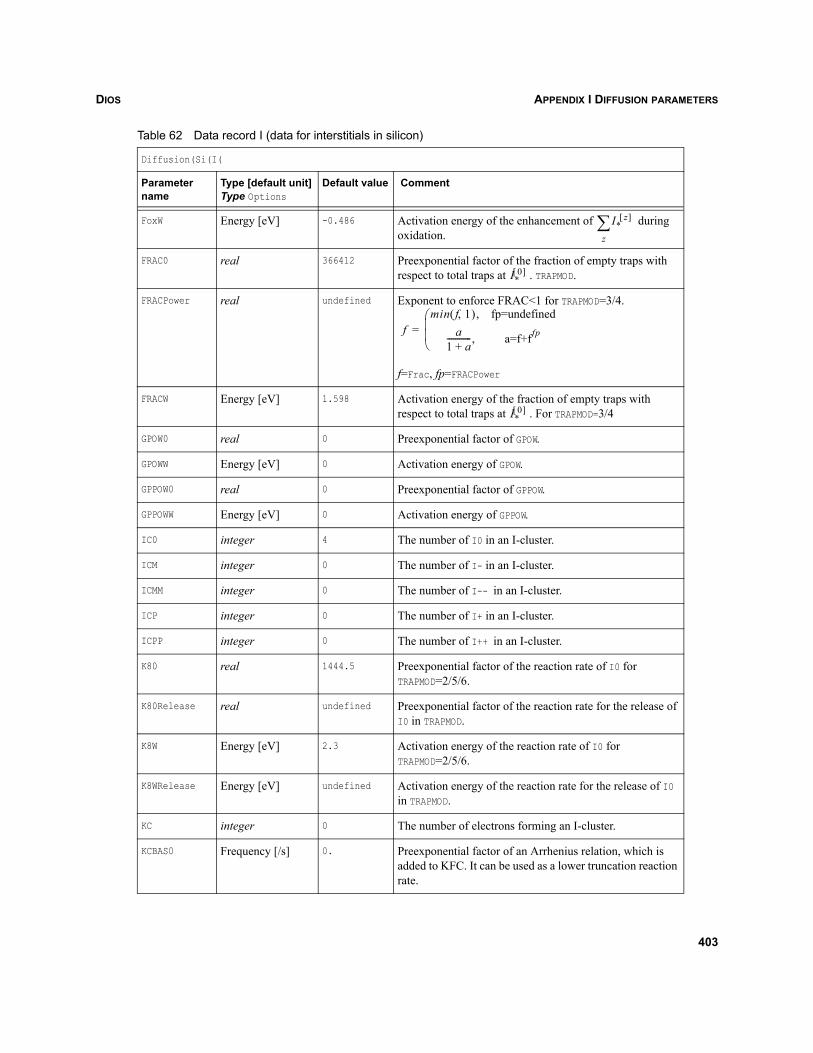
DIOS APPENDIX I DIFFUSION PARAMETERS
FoxW Energy [eV] -0.486 Activation energy of the enhancement of during oxidation.
FRAC0 real 366412 Preexponential factor of the fraction of empty traps with respect to total traps at . TRAPMOD.
FRACPower real undefined Exponent to enforce FRAC<1 for TRAPMOD=3/4.
f=Frac, fp=FRACPower
FRACW Energy [eV] 1.598 Activation energy of the fraction of empty traps with respect to total traps at . For TRAPMOD=3/4
GPOW0 real 0 Preexponential factor of GPOW.
GPOWW Energy [eV] 0 Activation energy of GPOW.
GPPOW0 real 0 Preexponential factor of GPPOW.
GPPOWW Energy [eV] 0 Activation energy of GPPOW.
IC0 integer 4 The number of I0 in an I-cluster.
ICM integer 0 The number of I- in an I-cluster.
ICMM integer 0 The number of I-- in an I-cluster.
ICP integer 0 The number of I+ in an I-cluster.
ICPP integer 0 The number of I++ in an I-cluster.
K80 real 1444.5 Preexponential factor of the reaction rate of I0 for TRAPMOD=2/5/6.
K80Release real undefined Preexponential factor of the reaction rate for the release of I0 in TRAPMOD.
K8W Energy [eV] 2.3 Activation energy of the reaction rate of I0 for TRAPMOD=2/5/6.
K8WRelease Energy [eV] undefined Activation energy of the reaction rate for the release of I0 in TRAPMOD.
KC integer 0 The number of electrons forming an I-cluster.
KCBAS0 Frequency [/s] 0. Preexponential factor of an Arrhenius relation, which is added to KFC. It can be used as a lower truncation reaction rate.
Table 62 Data record I (data for interstitials in silicon)
Diffusion(Si(I(
Parameter name
Type [default unit]Type Options
Default value Comment
I*z[ ]
z∑
I*0[ ]
fmin f 1,( ) fp=undefined,
a1 a+------------ a=f+ffp,
⎝⎜⎜⎛
=
I*0[ ]
403
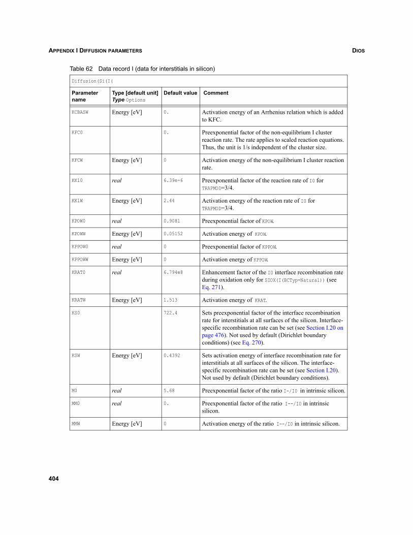
DIOSAPPENDIX I DIFFUSION PARAMETERS
KCBASW Energy [eV] 0. Activation energy of an Arrhenius relation which is added to KFC.
KFC0 0. Preexponential factor of the non-equilibrium I cluster reaction rate. The rate applies to scaled reaction equations. Thus, the unit is 1/s independent of the cluster size.
KFCW Energy [eV] 0 Activation energy of the non-equilibrium I cluster reaction rate.
KK10 real 6.39e-6 Preexponential factor of the reaction rate of I0 for TRAPMOD=3/4.
KK1W Energy [eV] 2.44 Activation energy of the reaction rate of I0 for TRAPMOD=3/4.
KPOW0 real 0.9081 Preexponential factor of KPOW.
KPOWW Energy [eV] 0.05152 Activation energy of KPOW.
KPPOW0 real 0 Preexponential factor of KPPOW.
KPPOWW Energy [eV] 0 Activation energy of KPPOW.
KRAT0 real 6.794e8 Enhancement factor of the I0 interface recombination rate during oxidation only for SIOX(I(BCTyp=Natural)) (see Eq. 271).
KRATW Energy [eV] 1.513 Activation energy of KRAT.
KS0 722.4 Sets preexponential factor of the interface recombination rate for interstitials at all surfaces of the silicon. Interface-specific recombination rate can be set (see Section I.20 on page 476). Not used by default (Dirichlet boundary conditions) (see Eq. 270).
KSW Energy [eV] 0.4392 Sets activation energy of interface recombination rate for interstitials at all surfaces of the silicon. The interface-specific recombination rate can be set (see Section I.20). Not used by default (Dirichlet boundary conditions).
M0 real 5.68 Preexponential factor of the ratio I-/I0 in intrinsic silicon.
MM0 real 0. Preexponential factor of the ratio I--/I0 in intrinsic silicon.
MMW Energy [eV] 0 Activation energy of the ratio I--/I0 in intrinsic silicon.
Table 62 Data record I (data for interstitials in silicon)
Diffusion(Si(I(
Parameter name
Type [default unit]Type Options
Default value Comment
404
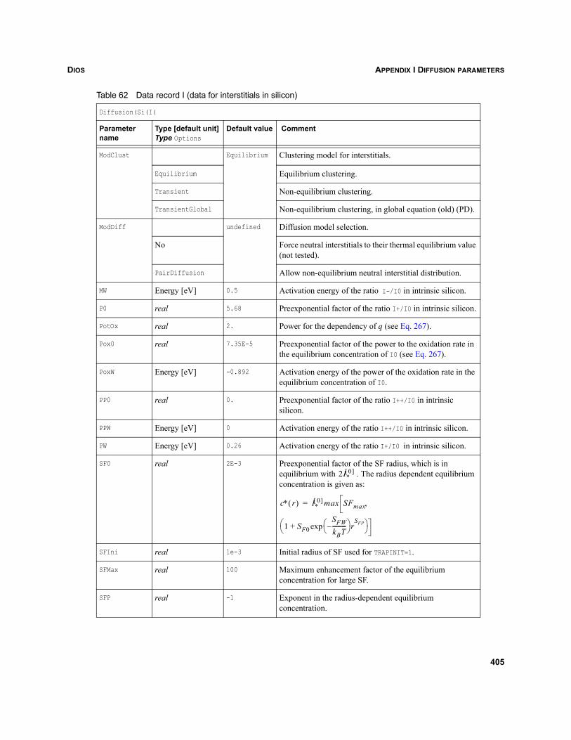
DIOS APPENDIX I DIFFUSION PARAMETERS
ModClust Equilibrium Clustering model for interstitials.
Equilibrium Equilibrium clustering.
Transient Non-equilibrium clustering.
TransientGlobal Non-equilibrium clustering, in global equation (old) (PD).
ModDiff undefined Diffusion model selection.
No Force neutral interstitials to their thermal equilibrium value (not tested).
PairDiffusion Allow non-equilibrium neutral interstitial distribution.
MW Energy [eV] 0.5 Activation energy of the ratio I-/I0 in intrinsic silicon.
P0 real 5.68 Preexponential factor of the ratio I+/I0 in intrinsic silicon.
PotOx real 2. Power for the dependency of q (see Eq. 267).
Pox0 real 7.35E-5 Preexponential factor of the power to the oxidation rate in the equilibrium concentration of I0 (see Eq. 267).
PoxW Energy [eV] -0.892 Activation energy of the power of the oxidation rate in the equilibrium concentration of I0.
PP0 real 0. Preexponential factor of the ratio I++/I0 in intrinsic silicon.
PPW Energy [eV] 0 Activation energy of the ratio I++/I0 in intrinsic silicon.
PW Energy [eV] 0.26 Activation energy of the ratio I+/I0 in intrinsic silicon.
SF0 real 2E-3 Preexponential factor of the SF radius, which is in equilibrium with . The radius dependent equilibrium concentration is given as:
SFIni real 1e-3 Initial radius of SF used for TRAPINIT=1.
SFMax real 100 Maximum enhancement factor of the equilibrium concentration for large SF.
SFP real -1 Exponent in the radius-dependent equilibrium concentration.
Table 62 Data record I (data for interstitials in silicon)
Diffusion(Si(I(
Parameter name
Type [default unit]Type Options
Default value Comment
2I*0[ ]
c∗ r( ) I*0[ ] max SFmax
1 SF0SFWkBT----------–⎝ ⎠
⎛ ⎞ rSFPexp+⎝ ⎠
⎛ ⎞
,=
405
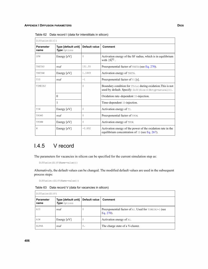
DIOSAPPENDIX I DIFFUSION PARAMETERS
I.4.5 V record
The parameters for vacancies in silicon can be specified for the current simulation step as:
Diffusion(Si(V(Name=value)))
Alternatively, the default values can be changed. The modified default values are used in the subsequentprocess steps:
Diffusion:(Si(V(Name=value)))
SFW Energy [eV] 0 Activation energy of the SF radius, which is in equilibrium with .
THETA0 real 151.55 Preexponential factor of THETA (see Eq. 270).
THETAW Energy [eV] 1.1849 Activation energy of THETA.
TI0 real -1 Preexponential factor of TI [s].
TIMEINJ 0 Boundary condition for ITotal during oxidation.This is not used by default. Specify: Diff(Siox(I(Bctyp=natural))).
0 Oxidation rate–dependent I0-injection.
1 Time-dependent I0-injection.
TIW Energy [eV] 0 Activation energy of TI.
TPOW0 real 0 Preexponential factor of TPOW.
TPOWW Energy [eV] 0 Activation energy of TPOW.
W Energy [eV] -0.892 Activation energy of the power of the oxidation rate in the equilibrium concentration of I0 (see Eq. 267).
Table 63 Data record V (data for vacancies in silicon)
Diffusion(Si(V(
Parameter name
Type [default unit]Type Options
Default value Comment
AI0 real 0 Preexponential factor of AI. Used for TIMEINJ=1 (see Eq. 270).
AIW Energy [eV] 0 Activation energy of AI.
ALPHA real 0. The charge state of a V-cluster.
Table 62 Data record I (data for interstitials in silicon)
Diffusion(Si(I(
Parameter name
Type [default unit]Type Options
Default value Comment
2I*0[ ]
406
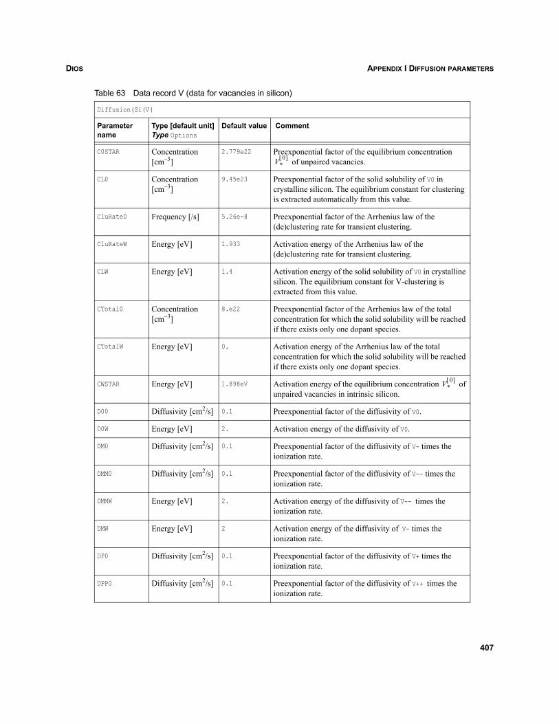
DIOS APPENDIX I DIFFUSION PARAMETERS
C0STAR Concentration [cm–3]
2.779e22 Preexponential factor of the equilibrium concentration of unpaired vacancies.
CL0 Concentration [cm–3]
9.45e23 Preexponential factor of the solid solubility of V0 in crystalline silicon. The equilibrium constant for clustering is extracted automatically from this value.
CluRate0 Frequency [/s] 5.26e-8 Preexponential factor of the Arrhenius law of the (de)clustering rate for transient clustering.
CluRateW Energy [eV] 1.933 Activation energy of the Arrhenius law of the (de)clustering rate for transient clustering.
CLW Energy [eV] 1.4 Activation energy of the solid solubility of V0 in crystalline silicon. The equilibrium constant for V-clustering is extracted from this value.
CTotal0 Concentration [cm–3]
8.e22 Preexponential factor of the Arrhenius law of the total concentration for which the solid solubility will be reached if there exists only one dopant species.
CTotalW Energy [eV] 0. Activation energy of the Arrhenius law of the total concentration for which the solid solubility will be reached if there exists only one dopant species.
CWSTAR Energy [eV] 1.898eV Activation energy of the equilibrium concentration of unpaired vacancies in intrinsic silicon.
D00 Diffusivity [cm2/s] 0.1 Preexponential factor of the diffusivity of V0.
D0W Energy [eV] 2. Activation energy of the diffusivity of V0.
DM0 Diffusivity [cm2/s] 0.1 Preexponential factor of the diffusivity of V- times the ionization rate.
DMM0 Diffusivity [cm2/s] 0.1 Preexponential factor of the diffusivity of V-- times the ionization rate.
DMMW Energy [eV] 2. Activation energy of the diffusivity of V-- times the ionization rate.
DMW Energy [eV] 2 Activation energy of the diffusivity of V- times the ionization rate.
DP0 Diffusivity [cm2/s] 0.1 Preexponential factor of the diffusivity of V+ times the ionization rate.
DPP0 Diffusivity [cm2/s] 0.1 Preexponential factor of the diffusivity of V++ times the ionization rate.
Table 63 Data record V (data for vacancies in silicon)
Diffusion(Si(V(
Parameter name
Type [default unit]Type Options
Default value Comment
V*0[ ]
V*0[ ]
407
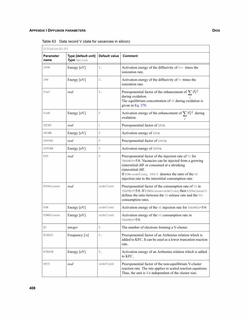
DIOSAPPENDIX I DIFFUSION PARAMETERS
DPPW Energy [eV] 2. Activation energy of the diffusivity of V++ times the ionization rate.
DPW Energy [eV] 2. Activation energy of the diffusivity of V+ times the ionization rate.
Fox0 real 0. Preexponential factor of the enhancement of during oxidation. The equilibrium concentration of V0 during oxidation is given in Eq. 270.
FoxW Energy [eV] 0 Activation energy of the enhancement of during oxidation.
GPOW0 real 1 Preexponential factor of GPOW.
GPOWW Energy [eV] 0 Activation energy of GPOW.
GPPOW0 real 0 Preexponential factor of GPPOW.
GPPOWW Energy [eV] 0 Activation energy of GPPOW.
K90 real 0 Preexponential factor of the injection rate of V0 for TRAPMOD=5/6. Vacancies can be injected from a growing (interstitial-)SF or consumed at a shrinking (interstitial-)SF. If K9W=undefined, K90>0 denotes the ratio of the V0 injection rate to the interstitial consumption rate.
K90Release real undefined Preexponential factor of the consumption rate of V0 in TRAPMOD=5/6. If K9WRelease=undefined, then K90Release>0 defines the ratio between the V0-release rate and the V0-consumption rates.
K9W Energy [eV] undefined Activation energy of the V0 injection rate for TRAPMOD=5/6
K9WRelease Energy [eV] undefined Activation energy of the V0 consumption rate in TRAPMOD=5/6
KC integer 0 The number of electrons forming a V-cluster.
KCBAS0 Frequency [/s] 0. Preexponential factor of an Arrhenius relation which is added to KFC. It can be used as a lower truncation reaction rate.
KCBASW Energy [eV] 0. Activation energy of an Arrhenius relation which is added to KFC.
KFC0 real undefined Preexponential factor of the non-equilibrium V-cluster reaction rate. The rate applies to scaled reaction equations. Thus, the unit is 1/s independent of the cluster size.
Table 63 Data record V (data for vacancies in silicon)
Diffusion(Si(V(
Parameter name
Type [default unit]Type Options
Default value Comment
V*z[ ]
z∑
V*z[ ]
z∑
408
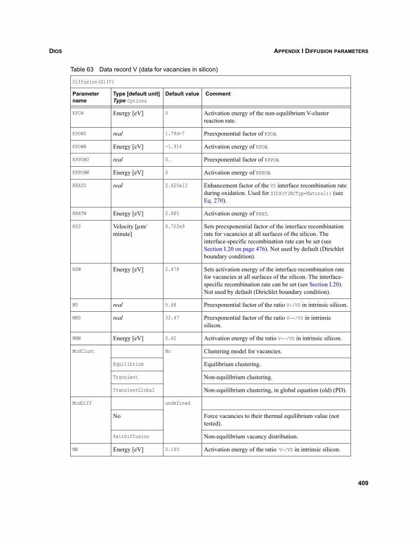
DIOS APPENDIX I DIFFUSION PARAMETERS
KFCW Energy [eV] 0 Activation energy of the non-equilibrium V-cluster reaction rate.
KPOW0 real 1.79d-7 Preexponential factor of KPOW.
KPOWW Energy [eV] -1.914 Activation energy of KPOW.
KPPOW0 real 0. Preexponential factor of KPPOW.
KPPOWW Energy [eV] 0 Activation energy of KPPOW.
KRAT0 real 2.620e12 Enhancement factor of the V0 interface recombination rate during oxidation. Used for SIOX(V(BCTyp=Natural)) (see Eq. 270).
KRATW Energy [eV] 2.885 Activation energy of KRAT.
KS0 Velocity [μm/minute]
6.702e9 Sets preexponential factor of the interface recombination rate for vacancies at all surfaces of the silicon. The interface-specific recombination rate can be set (see Section I.20 on page 476). Not used by default (Dirichlet boundary condition).
KSW Energy [eV] 2.478 Sets activation energy of the interface recombination rate for vacancies at all surfaces of the silicon. The interface-specific recombination rate can be set (see Section I.20). Not used by default (Dirichlet boundary condition).
M0 real 5.68 Preexponential factor of the ratio V-/V0 in intrinsic silicon.
MM0 real 32.47 Preexponential factor of the ratio V--/V0 in intrinsic silicon.
MMW Energy [eV] 0.62 Activation energy of the ratio V--/V0 in intrinsic silicon.
ModClust No Clustering model for vacancies.
Equilibrium Equilibrium clustering.
Transient Non-equilibrium clustering.
TransientGlobal Non-equilibrium clustering, in global equation (old) (PD).
ModDiff undefined
No Force vacancies to their thermal equilibrium value (not tested).
PairDiffusion Non-equilibrium vacancy distribution.
MW Energy [eV] 0.145 Activation energy of the ratio V-/V0 in intrinsic silicon.
Table 63 Data record V (data for vacancies in silicon)
Diffusion(Si(V(
Parameter name
Type [default unit]Type Options
Default value Comment
409
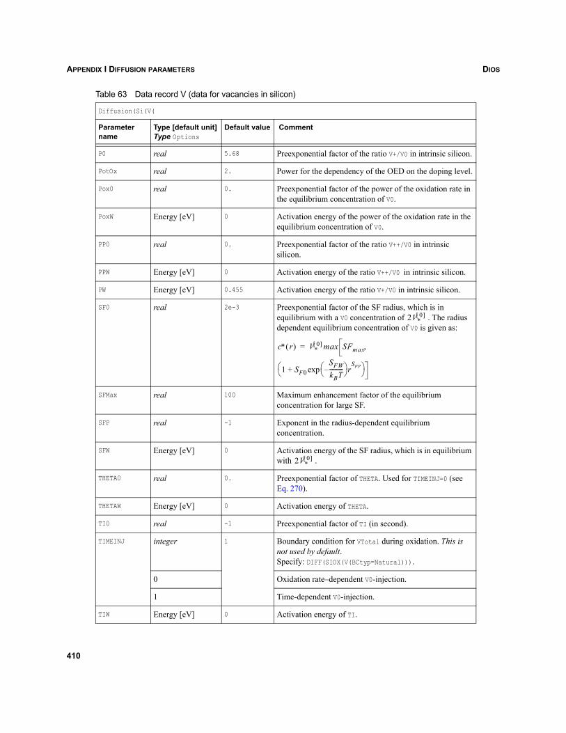
DIOSAPPENDIX I DIFFUSION PARAMETERS
P0 real 5.68 Preexponential factor of the ratio V+/V0 in intrinsic silicon.
PotOx real 2. Power for the dependency of the OED on the doping level.
Pox0 real 0. Preexponential factor of the power of the oxidation rate in the equilibrium concentration of V0.
PoxW Energy [eV] 0 Activation energy of the power of the oxidation rate in the equilibrium concentration of V0.
PP0 real 0. Preexponential factor of the ratio V++/V0 in intrinsic silicon.
PPW Energy [eV] 0 Activation energy of the ratio V++/V0 in intrinsic silicon.
PW Energy [eV] 0.455 Activation energy of the ratio V+/V0 in intrinsic silicon.
SF0 real 2e-3 Preexponential factor of the SF radius, which is in equilibrium with a V0 concentration of . The radius dependent equilibrium concentration of V0 is given as:
SFMax real 100 Maximum enhancement factor of the equilibrium concentration for large SF.
SFP real -1 Exponent in the radius-dependent equilibrium concentration.
SFW Energy [eV] 0 Activation energy of the SF radius, which is in equilibrium with .
THETA0 real 0. Preexponential factor of THETA. Used for TIMEINJ=0 (see Eq. 270).
THETAW Energy [eV] 0 Activation energy of THETA.
TI0 real -1 Preexponential factor of TI (in second).
TIMEINJ integer 1 Boundary condition for VTotal during oxidation. This is not used by default. Specify: DIFF(SIOX(V(BCtyp=Natural))).
0 Oxidation rate–dependent V0-injection.
1 Time-dependent V0-injection.
TIW Energy [eV] 0 Activation energy of TI.
Table 63 Data record V (data for vacancies in silicon)
Diffusion(Si(V(
Parameter name
Type [default unit]Type Options
Default value Comment
2V*0[ ]
c∗ r( ) V*0[ ] max SFmax
1 SF0SFWkBT----------–⎝ ⎠
⎛ ⎞ rSFPexp+⎝ ⎠
⎛ ⎞
,=
2V*0[ ]
410
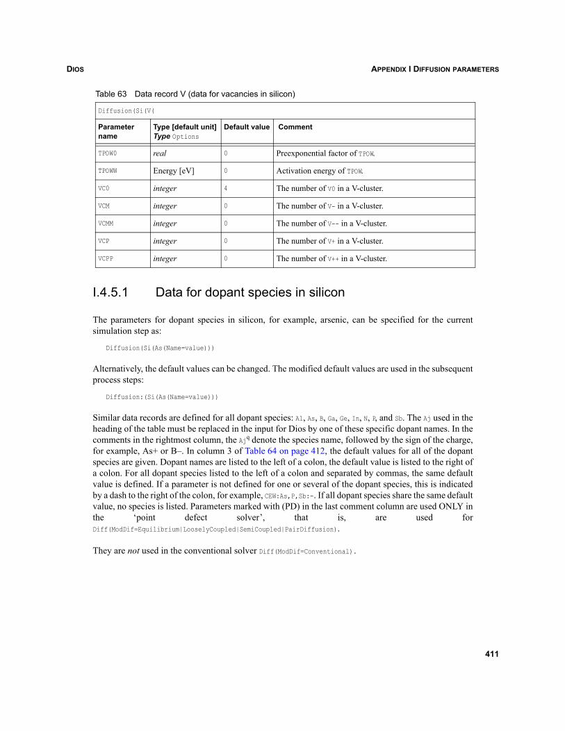
DIOS APPENDIX I DIFFUSION PARAMETERS
I.4.5.1 Data for dopant species in silicon
The parameters for dopant species in silicon, for example, arsenic, can be specified for the currentsimulation step as:
Diffusion(Si(As(Name=value)))
Alternatively, the default values can be changed. The modified default values are used in the subsequentprocess steps:
Diffusion:(Si(As(Name=value)))
Similar data records are defined for all dopant species: Al, As, B, Ga, Ge, In, N, P, and Sb. The Aj used in theheading of the table must be replaced in the input for Dios by one of these specific dopant names. In thecomments in the rightmost column, the Ajq denote the species name, followed by the sign of the charge,for example, As+ or B–. In column 3 of Table 64 on page 412, the default values for all of the dopantspecies are given. Dopant names are listed to the left of a colon, the default value is listed to the right ofa colon. For all dopant species listed to the left of a colon and separated by commas, the same defaultvalue is defined. If a parameter is not defined for one or several of the dopant species, this is indicatedby a dash to the right of the colon, for example, CEW:As,P,Sb:-. If all dopant species share the same defaultvalue, no species is listed. Parameters marked with (PD) in the last comment column are used ONLY inthe ‘point defect solver’, that is, are used forDiff(ModDif=Equilibrium|LooselyCoupled|SemiCoupled|PairDiffusion).
They are not used in the conventional solver Diff(ModDif=Conventional).
TPOW0 real 0 Preexponential factor of TPOW.
TPOWW Energy [eV] 0 Activation energy of TPOW.
VC0 integer 4 The number of V0 in a V-cluster.
VCM integer 0 The number of V- in a V-cluster.
VCMM integer 0 The number of V-- in a V-cluster.
VCP integer 0 The number of V+ in a V-cluster.
VCPP integer 0 The number of V++ in a V-cluster.
Table 63 Data record V (data for vacancies in silicon)
Diffusion(Si(V(
Parameter name
Type [default unit]Type Options
Default value Comment
411
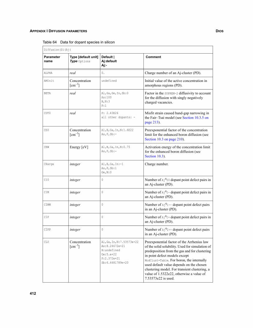
DIOSAPPENDIX I DIFFUSION PARAMETERS
Table 64 Data for dopant species in silicon
Diffusion(Si(Aj(
Parameter name
Type [default unit]Type Options
Default | Aj:defaultAj:-
Comment
ALPHA real 0. Charge number of an Aj-cluster (PD).
AMInit Concentration [cm–3]
undefined Initial value of the active concentration in amorphous regions (PD).
BETA real Al,Ga,Ge,In,Sb:0As:100B,N:3P:1
Factor in the SUPREM-2 diffusivity to account for the diffusion with singly negatively charged vacancies.
CDT0 real P: 2.43E26all other dopants: -
Misfit strain caused band-gap narrowing in the Fair–Tsai model (see Section 10.3.5 on page 213).
CE0 Concentration [cm–3]
Al,B,Ga,In,N:1.6E22As,P,Sb:-
Preexponential factor of the concentration limit for the enhanced boron diffusion (see Section 10.3 on page 210).
CEW Energy [eV] Al,B,Ga,In,N:0.75As,P,Sb:-
Activation energy of the concentration limit for the enhanced boron diffusion (see Section 10.3).
CHarge integer Al,B,Ga,In:-1As,P,Sb:1Ge,N:0
Charge number.
CI0 integer 0 Number of AjqI0 dopant point defect pairs in an Aj-cluster (PD).
CIM integer 0 Number of AjqI- dopant point defect pairs in an Aj-cluster (PD).
CIMM integer 0 Number of AjqI-- dopant point defect pairs in an Aj-cluster (PD).
CIP integer 0 Number of AjqI+ dopant point defect pairs in an Aj-cluster (PD).
CIPP integer 0 Number of AjqI++ dopant point defect pairs in an Aj-cluster (PD).
CL0 Concentration [cm–3]
Al,Ga,In,N:7.53573e+22As:8.24672e+21B:undefinedGe:5.e+22P:2.372e+21Sb:6.6481789e+20
Preexponential factor of the Arrhenius law of the solid solubility. Used for simulation of predeposition from the gas and for clustering in point defect models except ModClust=Table. For boron, the internally used default value depends on the chosen clustering model. For transient clustering, a value of 1.5322e22, otherwise a value of 7.53573e22 is used.
412
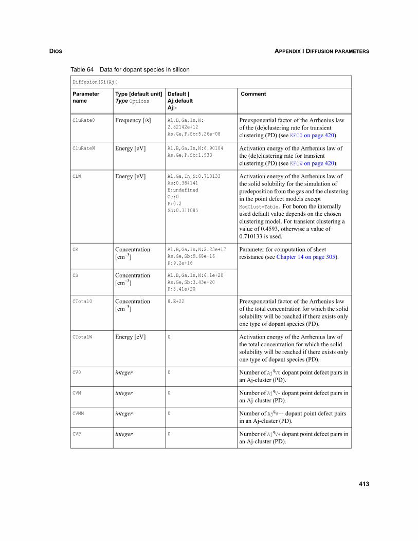
DIOS APPENDIX I DIFFUSION PARAMETERS
CluRate0 Frequency [/s] Al,B,Ga,In,N:2.82142e+12As,Ge,P,Sb:5.26e-08
Preexponential factor of the Arrhenius law of the (de)clustering rate for transient clustering (PD) (see KFC0 on page 420).
CluRateW Energy [eV] Al,B,Ga,In,N:6.90104As,Ge,P,Sb:1.933
Activation energy of the Arrhenius law of the (de)clustering rate for transient clustering (PD) (see KFCW on page 420).
CLW Energy [eV] Al,Ga,In,N:0.710133As:0.384141B:undefinedGe:0P:0.2Sb:0.311085
Activation energy of the Arrhenius law of the solid solubility for the simulation of predeposition from the gas and the clustering in the point defect models except ModClust=Table. For boron the internally used default value depends on the chosen clustering model. For transient clustering a value of 0.4593, otherwise a value of 0.710133 is used.
CR Concentration [cm–3]
Al,B,Ga,In,N:2.23e+17As,Ge,Sb:9.68e+16P:9.2e+16
Parameter for computation of sheet resistance (see Chapter 14 on page 305).
CS Concentration [cm–3]
Al,B,Ga,In,N:6.1e+20As,Ge,Sb:3.43e+20P:3.41e+20
CTotal0 Concentration [cm–3]
8.E+22 Preexponential factor of the Arrhenius law of the total concentration for which the solid solubility will be reached if there exists only one type of dopant species (PD).
CTotalW Energy [eV] 0 Activation energy of the Arrhenius law of the total concentration for which the solid solubility will be reached if there exists only one type of dopant species (PD).
CV0 integer 0 Number of AjqV0 dopant point defect pairs in an Aj-cluster (PD).
CVM integer 0 Number of AjqV- dopant point defect pairs in an Aj-cluster (PD).
CVMM integer 0 Number of AjqV-- dopant point defect pairs in an Aj-cluster (PD).
CVP integer 0 Number of AjqV+ dopant point defect pairs in an Aj-cluster (PD).
Table 64 Data for dopant species in silicon
Diffusion(Si(Aj(
Parameter name
Type [default unit]Type Options
Default | Aj:defaultAj:-
Comment
413
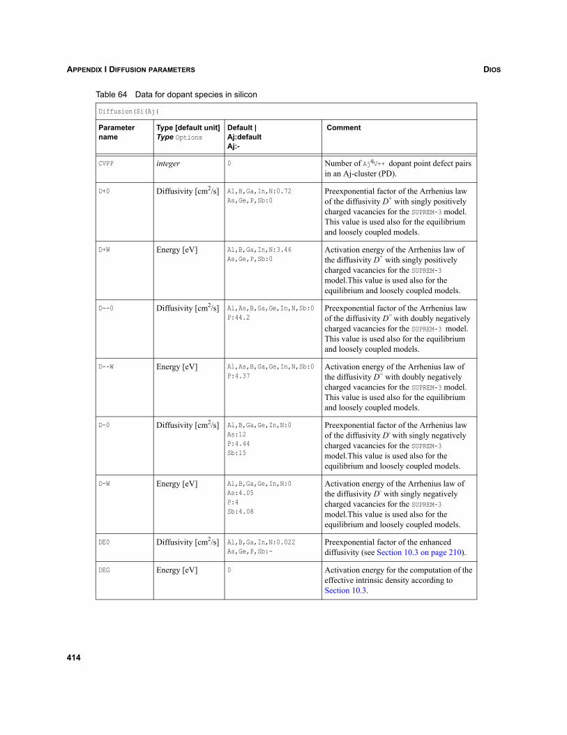
DIOSAPPENDIX I DIFFUSION PARAMETERS
CVPP integer 0 Number of AjqV++ dopant point defect pairs in an Aj-cluster (PD).
D+0 Diffusivity [cm2/s] Al,B,Ga,In,N:0.72As,Ge,P,Sb:0
Preexponential factor of the Arrhenius law of the diffusivity D+ with singly positively charged vacancies for the SUPREM-3 model. This value is used also for the equilibrium and loosely coupled models.
D+W Energy [eV] Al,B,Ga,In,N:3.46As,Ge,P,Sb:0
Activation energy of the Arrhenius law of the diffusivity D+ with singly positively charged vacancies for the SUPREM-3 model.This value is used also for the equilibrium and loosely coupled models.
D--0 Diffusivity [cm2/s] Al,As,B,Ga,Ge,In,N,Sb:0P:44.2
Preexponential factor of the Arrhenius law of the diffusivity D= with doubly negatively charged vacancies for the SUPREM-3 model. This value is used also for the equilibrium and loosely coupled models.
D--W Energy [eV] Al,As,B,Ga,Ge,In,N,Sb:0P:4.37
Activation energy of the Arrhenius law of the diffusivity D= with doubly negatively charged vacancies for the SUPREM-3 model. This value is used also for the equilibrium and loosely coupled models.
D-0 Diffusivity [cm2/s] Al,B,Ga,Ge,In,N:0As:12P:4.44Sb:15
Preexponential factor of the Arrhenius law of the diffusivity D- with singly negatively charged vacancies for the SUPREM-3 model.This value is used also for the equilibrium and loosely coupled models.
D-W Energy [eV] Al,B,Ga,Ge,In,N:0As:4.05P:4Sb:4.08
Activation energy of the Arrhenius law of the diffusivity D- with singly negatively charged vacancies for the SUPREM-3 model.This value is used also for the equilibrium and loosely coupled models.
DE0 Diffusivity [cm2/s] Al,B,Ga,In,N:0.022As,Ge,P,Sb:-
Preexponential factor of the enhanced diffusivity (see Section 10.3 on page 210).
DEG Energy [eV] 0 Activation energy for the computation of the effective intrinsic density according to Section 10.3.
Table 64 Data for dopant species in silicon
Diffusion(Si(Aj(
Parameter name
Type [default unit]Type Options
Default | Aj:defaultAj:-
Comment
414
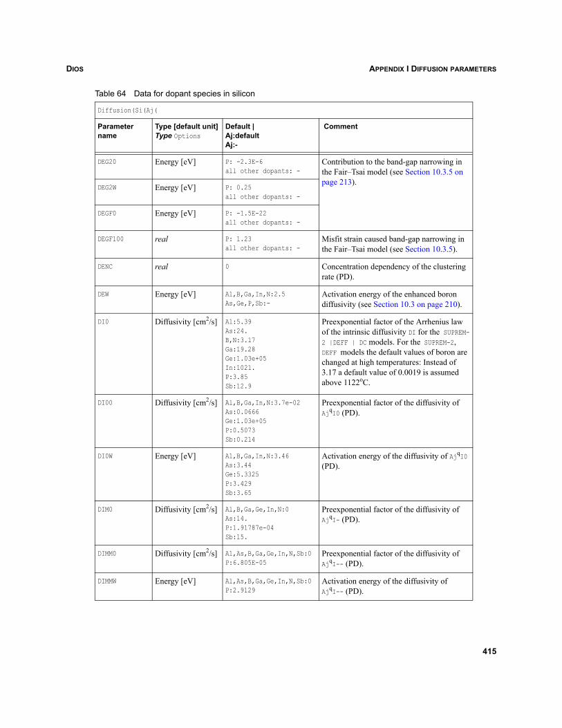
DIOS APPENDIX I DIFFUSION PARAMETERS
DEG20 Energy [eV] P: -2.3E-6all other dopants: -
Contribution to the band-gap narrowing in the Fair–Tsai model (see Section 10.3.5 on page 213).
DEG2W Energy [eV] P: 0.25all other dopants: -
DEGF0 Energy [eV] P: -1.5E-22all other dopants: -
DEGF100 real P: 1.23all other dopants: -
Misfit strain caused band-gap narrowing in the Fair–Tsai model (see Section 10.3.5).
DENC real 0 Concentration dependency of the clustering rate (PD).
DEW Energy [eV] Al,B,Ga,In,N:2.5As,Ge,P,Sb:-
Activation energy of the enhanced boron diffusivity (see Section 10.3 on page 210).
DI0 Diffusivity [cm2/s] Al:5.39As:24.B,N:3.17Ga:19.28Ge:1.03e+05In:1021.P:3.85Sb:12.9
Preexponential factor of the Arrhenius law of the intrinsic diffusivity DI for the SUPREM-2 |DEFF | DC models. For the SUPREM-2, DEFF models the default values of boron are changed at high temperatures: Instead of 3.17 a default value of 0.0019 is assumed above 1122oC.
DI00 Diffusivity [cm2/s] Al,B,Ga,In,N:3.7e-02As:0.0666Ge:1.03e+05P:0.5073Sb:0.214
Preexponential factor of the diffusivity of AjqI0 (PD).
DI0W Energy [eV] Al,B,Ga,In,N:3.46As:3.44Ge:5.3325P:3.429Sb:3.65
Activation energy of the diffusivity of AjqI0 (PD).
DIM0 Diffusivity [cm2/s] Al,B,Ga,Ge,In,N:0As:14.P:1.91787e-04Sb:15.
Preexponential factor of the diffusivity of AjqI- (PD).
DIMM0 Diffusivity [cm2/s] Al,As,B,Ga,Ge,In,N,Sb:0P:6.805E-05
Preexponential factor of the diffusivity of AjqI-- (PD).
DIMMW Energy [eV] Al,As,B,Ga,Ge,In,N,Sb:0P:2.9129
Activation energy of the diffusivity of AjqI-- (PD).
Table 64 Data for dopant species in silicon
Diffusion(Si(Aj(
Parameter name
Type [default unit]Type Options
Default | Aj:defaultAj:-
Comment
415
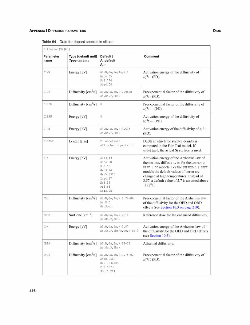
DIOSAPPENDIX I DIFFUSION PARAMETERS
DIMW Energy [eV] Al,B,Ga,Ge,In,N:0As:4.05P:2.774Sb:4.08
Activation energy of the diffusivity of AjqI- (PD).
DIP0 Diffusivity [cm2/s] Al,B,Ga,In,N:2.9618As,Ge,P,Sb:0
Preexponential factor of the diffusivity of AjqI+ (PD).
DIPP0 Diffusivity [cm2/s] 0 Preexponential factor of the diffusivity of AjqI++ (PD).
DIPPW Energy [eV] 0 Activation energy of the diffusivity of AjqI++ (PD).
DIPW Energy [eV] Al,B,Ga,In,N:3.625As,Ge,P,Sb:0
Activation energy of the diffusivity of AjqI+ (PD).
DISTOF Length [μm] P: undefinedall other dopants: -
Depth at which the surface density is computed in the Fair-Tsai model. If undefined, the actual Si surface is used.
DIW Energy [eV] Al:3.43As:4.08B:3.59Ga:3.74Ge:5.3325In:4.37N:3.59P:3.66Sb:3.98
Activation energy of the Arrhenius law of the intrinsic diffusivity DI for the SUPREM-2 | DEFF | DC models. For the SUPREM-2 | DEFF models the default values of boron are changed at high temperatures: Instead of 3.57, a default value of 2.7 is assumed above 1122oC.
DO0 Diffusivity [cm2/s] Al,B,Ga,In,N:1.2e-06As,P:0Ge,Sb:1.
Preexponential factor of the Arrhenius law of the diffusivity for the OED and ORD effects (see Section 10.3 on page 210).
DOSE SurConc [cm–2] Al,B,Ga,In,N:2E14As,Ge,P,Sb:-
Reference dose for the enhanced diffusivity.
DOW Energy [eV] Al,B,Ga,In,N:1.87As,Ge,P,Sb:As,Ge,P,Sb:0
Activation energy of the Arrhenius law of the diffusivity for the OED and ORD effects (see Section 10.3).
DRTA Diffusivity [cm2/s] Al,B,Ga,In,N:2E-12As,Ge,P,Sb:-
Athermal diffusivity.
DV00 Diffusivity [cm2/s] Al,B,Ga,In,N:3.7e-02As:0.0666Ge:1.03e+05P:0.5073Sb: 0.214
Preexponential factor of the diffusivity of AjqV0 (PD).
Table 64 Data for dopant species in silicon
Diffusion(Si(Aj(
Parameter name
Type [default unit]Type Options
Default | Aj:defaultAj:-
Comment
416
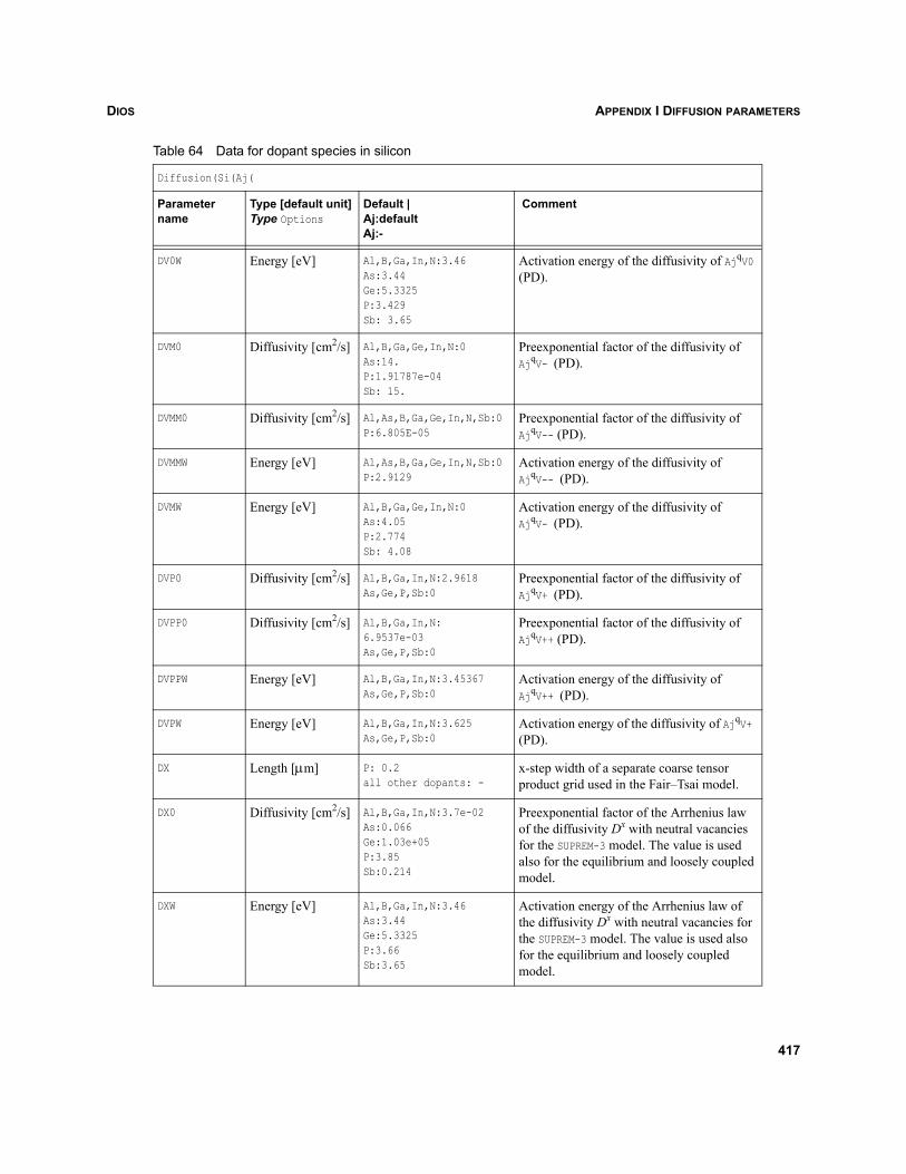
DIOS APPENDIX I DIFFUSION PARAMETERS
DV0W Energy [eV] Al,B,Ga,In,N:3.46As:3.44Ge:5.3325P:3.429Sb: 3.65
Activation energy of the diffusivity of AjqV0 (PD).
DVM0 Diffusivity [cm2/s] Al,B,Ga,Ge,In,N:0As:14.P:1.91787e-04Sb: 15.
Preexponential factor of the diffusivity of AjqV- (PD).
DVMM0 Diffusivity [cm2/s] Al,As,B,Ga,Ge,In,N,Sb:0P:6.805E-05
Preexponential factor of the diffusivity of AjqV-- (PD).
DVMMW Energy [eV] Al,As,B,Ga,Ge,In,N,Sb:0P:2.9129
Activation energy of the diffusivity of AjqV-- (PD).
DVMW Energy [eV] Al,B,Ga,Ge,In,N:0As:4.05P:2.774Sb: 4.08
Activation energy of the diffusivity of AjqV- (PD).
DVP0 Diffusivity [cm2/s] Al,B,Ga,In,N:2.9618As,Ge,P,Sb:0
Preexponential factor of the diffusivity of AjqV+ (PD).
DVPP0 Diffusivity [cm2/s] Al,B,Ga,In,N:6.9537e-03As,Ge,P,Sb:0
Preexponential factor of the diffusivity of AjqV++ (PD).
DVPPW Energy [eV] Al,B,Ga,In,N:3.45367As,Ge,P,Sb:0
Activation energy of the diffusivity of AjqV++ (PD).
DVPW Energy [eV] Al,B,Ga,In,N:3.625As,Ge,P,Sb:0
Activation energy of the diffusivity of AjqV+ (PD).
DX Length [μm] P: 0.2all other dopants: -
x-step width of a separate coarse tensor product grid used in the Fair–Tsai model.
DX0 Diffusivity [cm2/s] Al,B,Ga,In,N:3.7e-02As:0.066Ge:1.03e+05P:3.85Sb:0.214
Preexponential factor of the Arrhenius law of the diffusivity Dx with neutral vacancies for the SUPREM-3 model. The value is used also for the equilibrium and loosely coupled model.
DXW Energy [eV] Al,B,Ga,In,N:3.46As:3.44Ge:5.3325P:3.66Sb:3.65
Activation energy of the Arrhenius law of the diffusivity Dx with neutral vacancies for the SUPREM-3 model. The value is used also for the equilibrium and loosely coupled model.
Table 64 Data for dopant species in silicon
Diffusion(Si(Aj(
Parameter name
Type [default unit]Type Options
Default | Aj:defaultAj:-
Comment
417
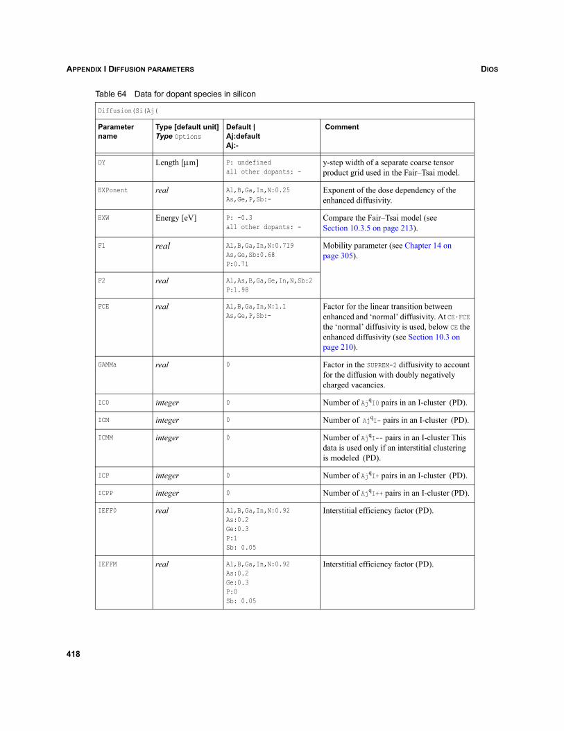
DIOSAPPENDIX I DIFFUSION PARAMETERS
DY Length [μm] P: undefinedall other dopants: -
y-step width of a separate coarse tensor product grid used in the Fair–Tsai model.
EXPonent real Al,B,Ga,In,N:0.25As,Ge,P,Sb:-
Exponent of the dose dependency of the enhanced diffusivity.
EXW Energy [eV] P: -0.3all other dopants: -
Compare the Fair–Tsai model (see Section 10.3.5 on page 213).
F1 real Al,B,Ga,In,N:0.719As,Ge,Sb:0.68P:0.71
Mobility parameter (see Chapter 14 on page 305).
F2 real Al,As,B,Ga,Ge,In,N,Sb:2P:1.98
FCE real Al,B,Ga,In,N:1.1As,Ge,P,Sb:-
Factor for the linear transition between enhanced and ‘normal’ diffusivity. At CE·FCE the ‘normal’ diffusivity is used, below CE the enhanced diffusivity (see Section 10.3 on page 210).
GAMMa real 0 Factor in the SUPREM-2 diffusivity to account for the diffusion with doubly negatively charged vacancies.
IC0 integer 0 Number of AjqI0 pairs in an I-cluster (PD).
ICM integer 0 Number of AjqI- pairs in an I-cluster (PD).
ICMM integer 0 Number of AjqI-- pairs in an I-cluster This data is used only if an interstitial clustering is modeled (PD).
ICP integer 0 Number of AjqI+ pairs in an I-cluster (PD).
ICPP integer 0 Number of AjqI++ pairs in an I-cluster (PD).
IEFF0 real Al,B,Ga,In,N:0.92As:0.2Ge:0.3P:1Sb: 0.05
Interstitial efficiency factor (PD).
IEFFM real Al,B,Ga,In,N:0.92As:0.2Ge:0.3P:0Sb: 0.05
Interstitial efficiency factor (PD).
Table 64 Data for dopant species in silicon
Diffusion(Si(Aj(
Parameter name
Type [default unit]Type Options
Default | Aj:defaultAj:-
Comment
418
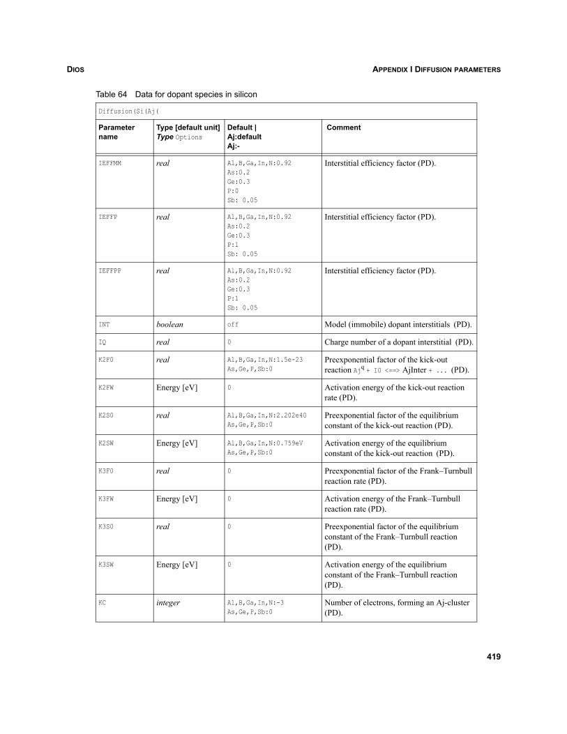
DIOS APPENDIX I DIFFUSION PARAMETERS
IEFFMM real Al,B,Ga,In,N:0.92As:0.2Ge:0.3P:0Sb: 0.05
Interstitial efficiency factor (PD).
IEFFP real Al,B,Ga,In,N:0.92As:0.2Ge:0.3P:1Sb: 0.05
Interstitial efficiency factor (PD).
IEFFPP real Al,B,Ga,In,N:0.92As:0.2Ge:0.3P:1Sb: 0.05
Interstitial efficiency factor (PD).
INT boolean off Model (immobile) dopant interstitials (PD).
IQ real 0 Charge number of a dopant interstitial (PD).
K2F0 real Al,B,Ga,In,N:1.5e-23As,Ge,P,Sb:0
Preexponential factor of the kick-out reaction Ajq + I0 <==> AjInter + ... (PD).
K2FW Energy [eV] 0 Activation energy of the kick-out reaction rate (PD).
K2S0 real Al,B,Ga,In,N:2.202e40As,Ge,P,Sb:0
Preexponential factor of the equilibrium constant of the kick-out reaction (PD).
K2SW Energy [eV] Al,B,Ga,In,N:0.759eVAs,Ge,P,Sb:0
Activation energy of the equilibrium constant of the kick-out reaction (PD).
K3F0 real 0 Preexponential factor of the Frank–Turnbull reaction rate (PD).
K3FW Energy [eV] 0 Activation energy of the Frank–Turnbull reaction rate (PD).
K3S0 real 0 Preexponential factor of the equilibrium constant of the Frank–Turnbull reaction (PD).
K3SW Energy [eV] 0 Activation energy of the equilibrium constant of the Frank–Turnbull reaction (PD).
KC integer Al,B,Ga,In,N:-3As,Ge,P,Sb:0
Number of electrons, forming an Aj-cluster (PD).
Table 64 Data for dopant species in silicon
Diffusion(Si(Aj(
Parameter name
Type [default unit]Type Options
Default | Aj:defaultAj:-
Comment
419
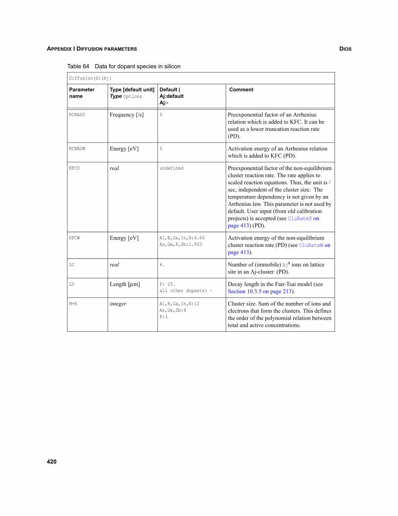
DIOSAPPENDIX I DIFFUSION PARAMETERS
KCBAS0 Frequency [/s] 0 Preexponential factor of an Arrhenius relation which is added to KFC. It can be used as a lower truncation reaction rate (PD).
KCBASW Energy [eV] 0 Activation energy of an Arrhenius relation which is added to KFC (PD).
KFC0 real undefined Preexponential factor of the non-equilibrium cluster reaction rate. The rate applies to scaled reaction equations. Thus, the unit is /sec, independent of the cluster size. The temperature dependency is not given by an Arrhenius law. This parameter is not used by default. User input (from old calibration projects) is accepted (see CluRate0 on page 413) (PD).
KFCW Energy [eV] Al,B,Ga,In,N:4.64As,Ge,P,Sb:1.933
Activation energy of the non-equilibrium cluster reaction rate (PD) (see CluRateW on page 413).
LC real 6. Number of (immobile) Ajq ions on lattice site in an Aj-cluster (PD).
LV Length [μm] P: 25.all other dopants: -
Decay length in the Fair-Tsai model (see Section 10.3.5 on page 213).
M+K integer Al,B,Ga,In,N:12As,Ge,Sb:4P:3
Cluster size. Sum of the number of ions and electrons that form the clusters. This defines the order of the polynomial relation between total and active concentrations.
Table 64 Data for dopant species in silicon
Diffusion(Si(Aj(
Parameter name
Type [default unit]Type Options
Default | Aj:defaultAj:-
Comment
420
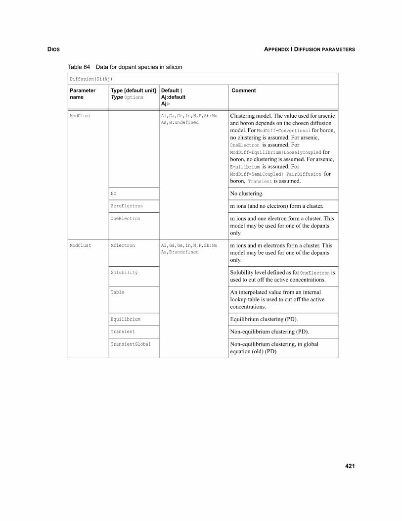
DIOS APPENDIX I DIFFUSION PARAMETERS
ModClust Al,Ga,Ge,In,N,P,Sb:NoAs,B:undefined
Clustering model. The value used for arsenic and boron depends on the chosen diffusion model. For ModDiff=Conventional for boron, no clustering is assumed. For arsenic, OneElectron is assumed. For ModDiff=Equilibrium|LooselyCoupled for boron, no clustering is assumed. For arsenic, Equilibrium is assumed. For ModDiff=SemiCoupled| PairDiffusion for boron, Transient is assumed.
No No clustering.
ZeroElectron m ions (and no electron) form a cluster.
OneElectron m ions and one electron form a cluster. This model may be used for one of the dopants only.
ModClust MElectron Al,Ga,Ge,In,N,P,Sb:NoAs,B:undefined
m ions and m electrons form a cluster. This model may be used for one of the dopants only.
Solubility Solubility level defined as for OneElectron is used to cut off the active concentrations.
Table An interpolated value from an internal lookup table is used to cut off the active concentrations.
Equilibrium Equilibrium clustering (PD).
Transient Non-equilibrium clustering (PD).
TransientGlobal Non-equilibrium clustering, in global equation (old) (PD).
Table 64 Data for dopant species in silicon
Diffusion(Si(Aj(
Parameter name
Type [default unit]Type Options
Default | Aj:defaultAj:-
Comment
421
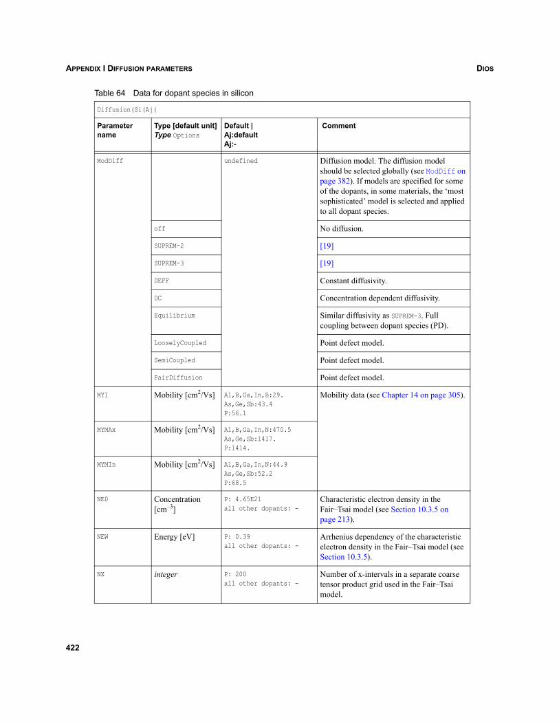
DIOSAPPENDIX I DIFFUSION PARAMETERS
ModDiff undefined Diffusion model. The diffusion model should be selected globally (see ModDiff on page 382). If models are specified for some of the dopants, in some materials, the ‘most sophisticated’ model is selected and applied to all dopant species.
off No diffusion.
SUPREM-2 [19]
SUPREM-3 [19]
DEFF Constant diffusivity.
DC Concentration dependent diffusivity.
Equilibrium Similar diffusivity as SUPREM-3. Full coupling between dopant species (PD).
LooselyCoupled Point defect model.
SemiCoupled Point defect model.
PairDiffusion Point defect model.
MY1 Mobility [cm2/Vs] Al,B,Ga,In,B:29.As,Ge,Sb:43.4P:56.1
Mobility data (see Chapter 14 on page 305).
MYMAx Mobility [cm2/Vs] Al,B,Ga,In,N:470.5As,Ge,Sb:1417.P:1414.
MYMIn Mobility [cm2/Vs] Al,B,Ga,In,N:44.9As,Ge,Sb:52.2P:68.5
NE0 Concentration [cm–3]
P: 4.65E21all other dopants: -
Characteristic electron density in the Fair–Tsai model (see Section 10.3.5 on page 213).
NEW Energy [eV] P: 0.39all other dopants: -
Arrhenius dependency of the characteristic electron density in the Fair–Tsai model (see Section 10.3.5).
NX integer P: 200all other dopants: -
Number of x-intervals in a separate coarse tensor product grid used in the Fair–Tsai model.
Table 64 Data for dopant species in silicon
Diffusion(Si(Aj(
Parameter name
Type [default unit]Type Options
Default | Aj:defaultAj:-
Comment
422
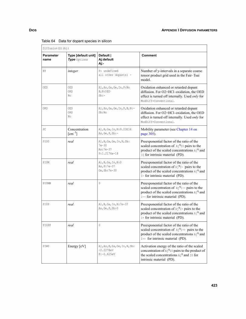
DIOS APPENDIX I DIFFUSION PARAMETERS
NY integer P: undefinedall other dopants: -
Number of y-intervals in a separate coarse tensor product grid used in the Fair–Tsai model.
OED OEDORDNo
Al,As,Ga,Ge,In,P:NoB,N:OEDSb:-
Oxidation enhanced or retarded dopant diffusion. For O2+HCl–oxidation, the OED effect is turned off internally. Used only for ModDiff=Conventional.
ORD OEDORDNo
Al,As,Ga,Ge,In,P,B,N:-Sb:No
Oxidation enhanced or retarded dopant diffusion. For O2+HCl–oxidation, the OED effect is turned off internally. Used only for ModDiff=Conventional.
PC Concentration [cm–3]
Al,B,Ga,In,N:9.23E16As,Ge,P,Sb:-
Mobility parameter (see Chapter 14 on page 305).
PI00 real Al,B,Ga,Ge,In,N,Sb:7e-30As:7e-37P:1.2176e-18
Preexponential factor of the ratio of the scaled concentration of AjqI0 pairs to the product of the scaled concentrations Ajq and I0 for intrinsic material (PD).
PI0M real Al,B,Ga,In,N:0As,P:7e-37Ge,Sb:7e-30
Preexponential factor of the ratio of the scaled concentration of AjqI- pairs to the product of the scaled concentrations Ajq and I- for intrinsic material (PD).
PI0MM real 0 Preexponential factor of the ratio of the scaled concentration of AjqI-- pairs to the product of the scaled concentrations Ajq and I-- for intrinsic material (PD).
PI0P real Al,B,Ga,In,N:7e-37As,Ge,P,Sb:0
Preexponential factor of the ratio of the scaled concentration of AjqI+ pairs to the product of the scaled concentrations Ajq and I+ for intrinsic material (PD).
PI0PP real 0 Preexponential factor of the ratio of the scaled concentration of AjqI++ pairs to the product of the scaled concentrations Ajq and I++ for intrinsic material (PD).
PIW0 Energy [eV] Al,As,B,Ga,Ge,In,N,Sb:-2.2278eVP:-0.625eV
Activation energy of the ratio of the scaled concentration of AjqI0 pairs to the product of the scaled concentrations Ajq and I0 for intrinsic material (PD).
Table 64 Data for dopant species in silicon
Diffusion(Si(Aj(
Parameter name
Type [default unit]Type Options
Default | Aj:defaultAj:-
Comment
423
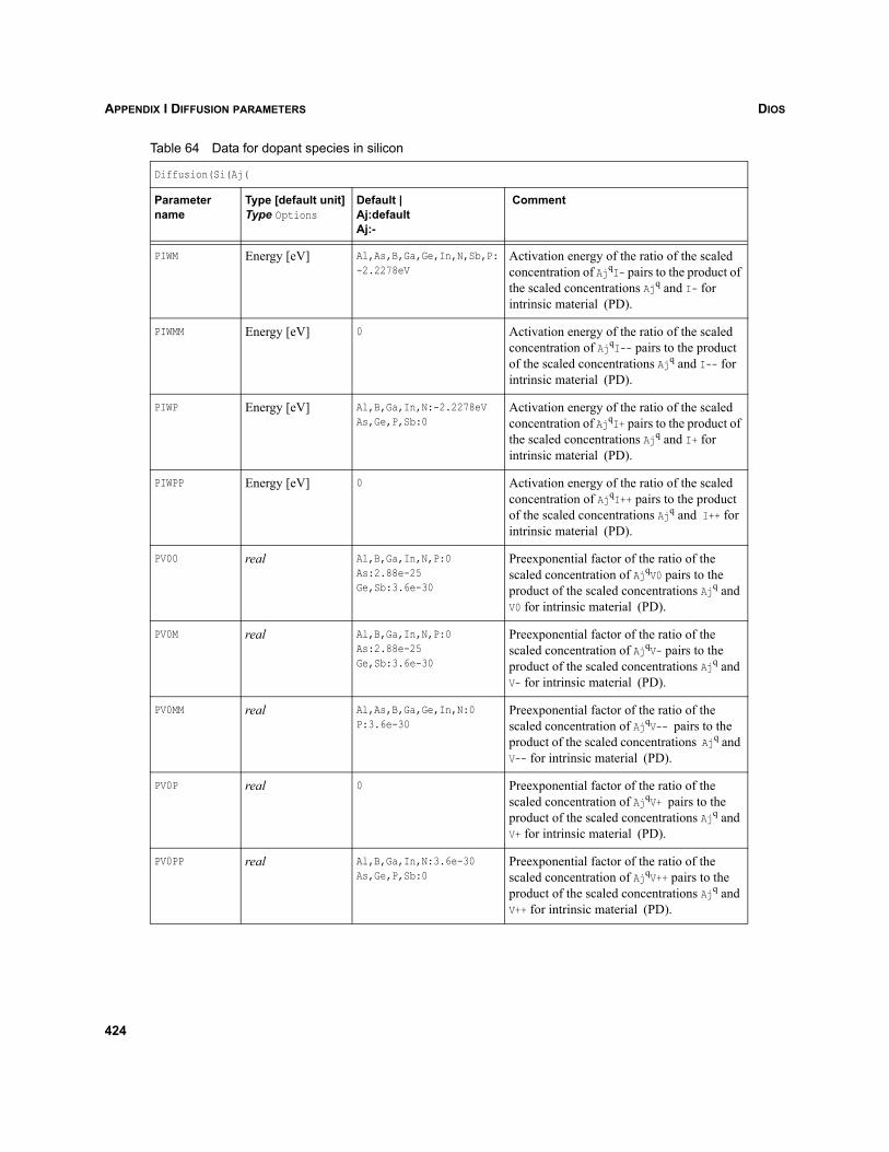
DIOSAPPENDIX I DIFFUSION PARAMETERS
PIWM Energy [eV] Al,As,B,Ga,Ge,In,N,Sb,P:-2.2278eV
Activation energy of the ratio of the scaled concentration of AjqI- pairs to the product of the scaled concentrations Ajq and I- for intrinsic material (PD).
PIWMM Energy [eV] 0 Activation energy of the ratio of the scaled concentration of AjqI-- pairs to the product of the scaled concentrations Ajq and I-- for intrinsic material (PD).
PIWP Energy [eV] Al,B,Ga,In,N:-2.2278eVAs,Ge,P,Sb:0
Activation energy of the ratio of the scaled concentration of AjqI+ pairs to the product of the scaled concentrations Ajq and I+ for intrinsic material (PD).
PIWPP Energy [eV] 0 Activation energy of the ratio of the scaled concentration of AjqI++ pairs to the product of the scaled concentrations Ajq and I++ for intrinsic material (PD).
PV00 real Al,B,Ga,In,N,P:0As:2.88e-25Ge,Sb:3.6e-30
Preexponential factor of the ratio of the scaled concentration of AjqV0 pairs to the product of the scaled concentrations Ajq and V0 for intrinsic material (PD).
PV0M real Al,B,Ga,In,N,P:0As:2.88e-25Ge,Sb:3.6e-30
Preexponential factor of the ratio of the scaled concentration of AjqV- pairs to the product of the scaled concentrations Ajq and V- for intrinsic material (PD).
PV0MM real Al,As,B,Ga,Ge,In,N:0P:3.6e-30
Preexponential factor of the ratio of the scaled concentration of AjqV-- pairs to the product of the scaled concentrations Ajq and V-- for intrinsic material (PD).
PV0P real 0 Preexponential factor of the ratio of the scaled concentration of AjqV+ pairs to the product of the scaled concentrations Ajq and V+ for intrinsic material (PD).
PV0PP real Al,B,Ga,In,N:3.6e-30As,Ge,P,Sb:0
Preexponential factor of the ratio of the scaled concentration of AjqV++ pairs to the product of the scaled concentrations Ajq and V++ for intrinsic material (PD).
Table 64 Data for dopant species in silicon
Diffusion(Si(Aj(
Parameter name
Type [default unit]Type Options
Default | Aj:defaultAj:-
Comment
424
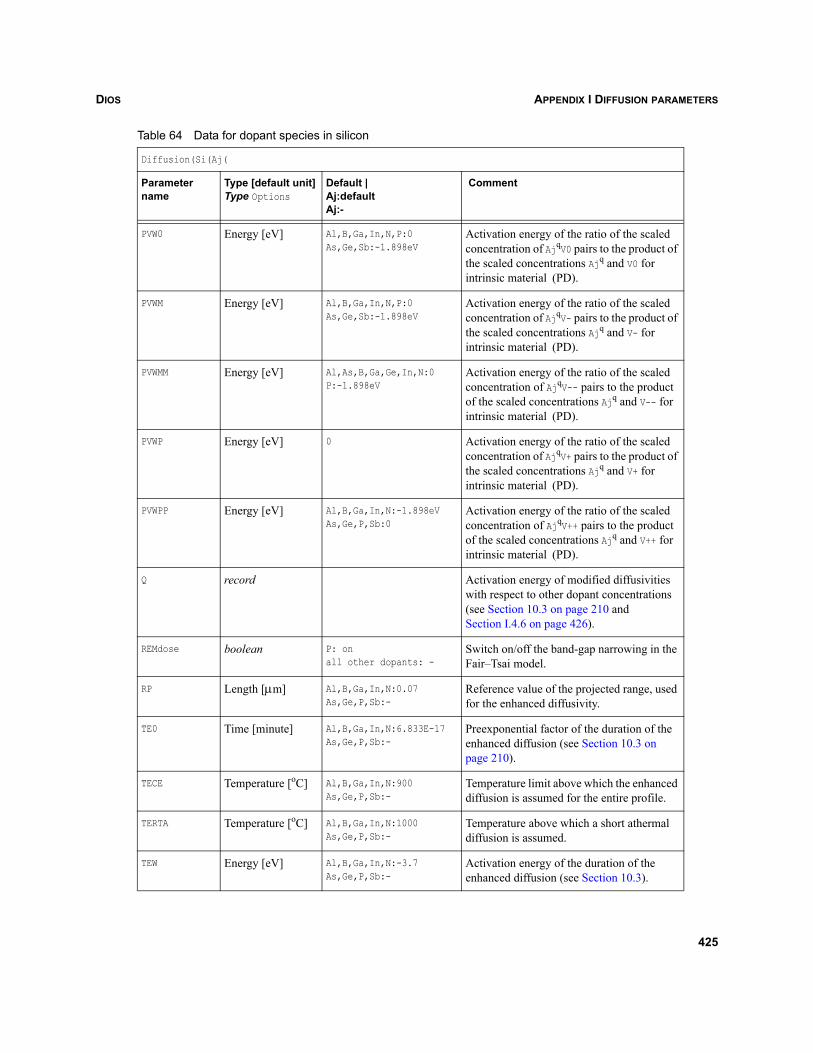
DIOS APPENDIX I DIFFUSION PARAMETERS
PVW0 Energy [eV] Al,B,Ga,In,N,P:0As,Ge,Sb:-1.898eV
Activation energy of the ratio of the scaled concentration of AjqV0 pairs to the product of the scaled concentrations Ajq and V0 for intrinsic material (PD).
PVWM Energy [eV] Al,B,Ga,In,N,P:0As,Ge,Sb:-1.898eV
Activation energy of the ratio of the scaled concentration of AjqV- pairs to the product of the scaled concentrations Ajq and V- for intrinsic material (PD).
PVWMM Energy [eV] Al,As,B,Ga,Ge,In,N:0P:-1.898eV
Activation energy of the ratio of the scaled concentration of AjqV-- pairs to the product of the scaled concentrations Ajq and V-- for intrinsic material (PD).
PVWP Energy [eV] 0 Activation energy of the ratio of the scaled concentration of AjqV+ pairs to the product of the scaled concentrations Ajq and V+ for intrinsic material (PD).
PVWPP Energy [eV] Al,B,Ga,In,N:-1.898eVAs,Ge,P,Sb:0
Activation energy of the ratio of the scaled concentration of AjqV++ pairs to the product of the scaled concentrations Ajq and V++ for intrinsic material (PD).
Q record Activation energy of modified diffusivities with respect to other dopant concentrations (see Section 10.3 on page 210 and Section I.4.6 on page 426).
REMdose boolean P: onall other dopants: -
Switch on/off the band-gap narrowing in the Fair–Tsai model.
RP Length [μm] Al,B,Ga,In,N:0.07As,Ge,P,Sb:-
Reference value of the projected range, used for the enhanced diffusivity.
TE0 Time [minute] Al,B,Ga,In,N:6.833E-17As,Ge,P,Sb:-
Preexponential factor of the duration of the enhanced diffusion (see Section 10.3 on page 210).
TECE Temperature [oC] Al,B,Ga,In,N:900As,Ge,P,Sb:-
Temperature limit above which the enhanced diffusion is assumed for the entire profile.
TERTA Temperature [oC] Al,B,Ga,In,N:1000As,Ge,P,Sb:-
Temperature above which a short athermal diffusion is assumed.
TEW Energy [eV] Al,B,Ga,In,N:-3.7As,Ge,P,Sb:-
Activation energy of the duration of the enhanced diffusion (see Section 10.3).
Table 64 Data for dopant species in silicon
Diffusion(Si(Aj(
Parameter name
Type [default unit]Type Options
Default | Aj:defaultAj:-
Comment
425
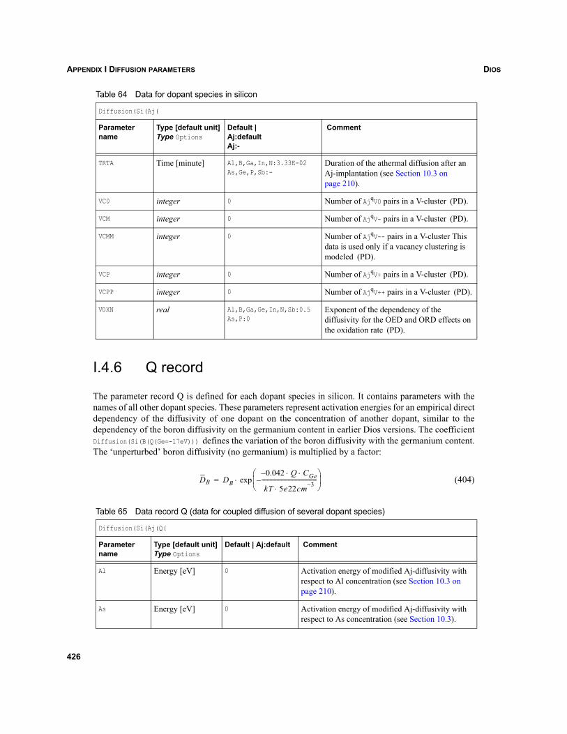
DIOSAPPENDIX I DIFFUSION PARAMETERS
I.4.6 Q record
The parameter record Q is defined for each dopant species in silicon. It contains parameters with thenames of all other dopant species. These parameters represent activation energies for an empirical directdependency of the diffusivity of one dopant on the concentration of another dopant, similar to thedependency of the boron diffusivity on the germanium content in earlier Dios versions. The coefficientDiffusion(Si(B(Q(Ge=-17eV))) defines the variation of the boron diffusivity with the germanium content.The ‘unperturbed’ boron diffusivity (no germanium) is multiplied by a factor:
(404)
TRTA Time [minute] Al,B,Ga,In,N:3.33E-02As,Ge,P,Sb:-
Duration of the athermal diffusion after an Aj-implantation (see Section 10.3 on page 210).
VC0 integer 0 Number of AjqV0 pairs in a V-cluster (PD).
VCM integer 0 Number of AjqV- pairs in a V-cluster (PD).
VCMM integer 0 Number of AjqV-- pairs in a V-cluster This data is used only if a vacancy clustering is modeled (PD).
VCP integer 0 Number of AjqV+ pairs in a V-cluster (PD).
VCPP integer 0 Number of AjqV++ pairs in a V-cluster (PD).
VOXN real Al,B,Ga,Ge,In,N,Sb:0.5As,P:0
Exponent of the dependency of the diffusivity for the OED and ORD effects on the oxidation rate (PD).
Table 65 Data record Q (data for coupled diffusion of several dopant species)
Diffusion(Si(Aj(Q(
Parameter name
Type [default unit]Type Options
Default | Aj:default Comment
Al Energy [eV] 0 Activation energy of modified Aj-diffusivity with respect to Al concentration (see Section 10.3 on page 210).
As Energy [eV] 0 Activation energy of modified Aj-diffusivity with respect to As concentration (see Section 10.3).
Table 64 Data for dopant species in silicon
Diffusion(Si(Aj(
Parameter name
Type [default unit]Type Options
Default | Aj:defaultAj:-
Comment
DB DB0.042 Q C⋅ ⋅– Ge
kT 5e22cm 3–⋅----------------------------------------–
⎝ ⎠⎜ ⎟⎛ ⎞
exp⋅=
426
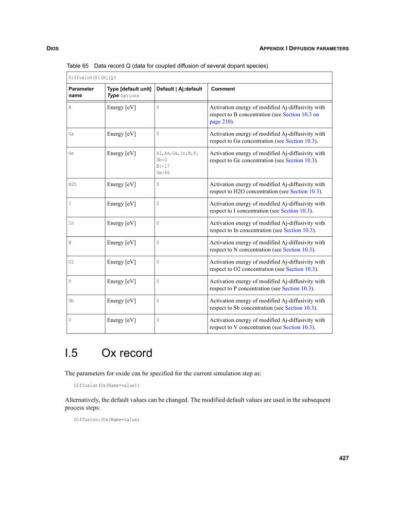
DIOS APPENDIX I DIFFUSION PARAMETERS
I.5 Ox recordThe parameters for oxide can be specified for the current simulation step as:
Diffusion(Ox(Name=value))
Alternatively, the default values can be changed. The modified default values are used in the subsequentprocess steps:
Diffusion:(Ox(Name=value)
B Energy [eV] 0 Activation energy of modified Aj-diffusivity with respect to B concentration (see Section 10.3 on page 210).
Ga Energy [eV] 0 Activation energy of modified Aj-diffusivity with respect to Ga concentration (see Section 10.3).
Ge Energy [eV] Al,As,Ga,In,N,P,Sb:0B:-17Ge:40
Activation energy of modified Aj-diffusivity with respect to Ge concentration (see Section 10.3).
H2O Energy [eV] 0 Activation energy of modified Aj-diffusivity with respect to H2O concentration (see Section 10.3).
I Energy [eV] 0 Activation energy of modified Aj-diffusivity with respect to I concentration (see Section 10.3).
In Energy [eV] 0 Activation energy of modified Aj-diffusivity with respect to In concentration (see Section 10.3).
N Energy [eV] 0 Activation energy of modified Aj-diffusivity with respect to N concentration (see Section 10.3).
O2 Energy [eV] 0 Activation energy of modified Aj-diffusivity with respect to O2 concentration (see Section 10.3).
P Energy [eV] 0 Activation energy of modified Aj-diffusivity with respect to P concentration (see Section 10.3).
Sb Energy [eV] 0 Activation energy of modified Aj-diffusivity with respect to Sb concentration (see Section 10.3).
V Energy [eV] 0 Activation energy of modified Aj-diffusivity with respect to V concentration (see Section 10.3).
Table 65 Data record Q (data for coupled diffusion of several dopant species)
Diffusion(Si(Aj(Q(
Parameter name
Type [default unit]Type Options
Default | Aj:default Comment
427
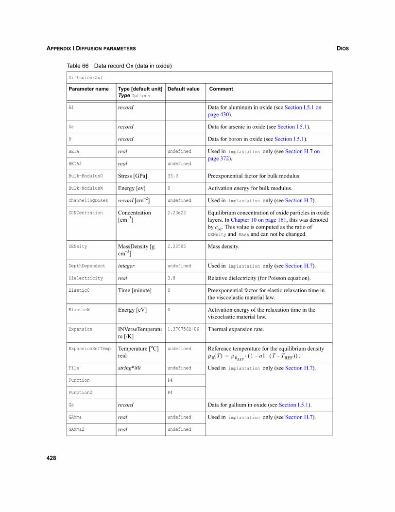
DIOSAPPENDIX I DIFFUSION PARAMETERS
Table 66 Data record Ox (data in oxide)
Diffusion(Ox(
Parameter name Type [default unit]Type Options
Default value Comment
Al record Data for aluminum in oxide (see Section I.5.1 on page 430).
As record Data for arsenic in oxide (see Section I.5.1).
B record Data for boron in oxide (see Section I.5.1).
BETA real undefined Used in implantation only (see Section H.7 on page 372).
BETA2 real undefined
Bulk-Modulus0 Stress [GPa] 33.0 Preexponential factor for bulk modulus.
Bulk-ModulusW Energy [ev] 0 Activation energy for bulk modulus.
ChannelingDoses record [cm–2] undefined Used in implantation only (see Section H.7).
CONCentration Concentration [cm–3]
2.23e22 Equilibrium concentration of oxide particles in oxide layers. In Chapter 10 on page 161, this was denoted by cox. This value is computed as the ratio of DENsity and Mass and can not be changed.
DENsity MassDensity [g cm–3]
2.22505 Mass density.
DepthDependent integer undefined Used in implantation only (see Section H.7).
Dielectricity real 3.8 Relative dielectricity (for Poisson equation).
Elastic0 Time [minute] 0 Preexponential factor for elastic relaxation time in the viscoelastic material law.
ElasticW Energy [eV] 0 Activation energy of the relaxation time in the viscoelastic material law.
Expansion INVerseTemperature [/K]
1.370756E-06 Thermal expansion rate.
ExpansionRefTemp Temperature [oC]real
undefined Reference temperature for the equilibrium density .
File string*80 undefined Used in implantation only (see Section H.7).
Function P4
Function2 P4
Ga record Data for gallium in oxide (see Section I.5.1).
GAMma real undefined Used in implantation only (see Section H.7).
GAMma2 real undefined
ρ0 T( ) ρ0REF1 a1 T TREF–( )⋅–( )⋅=
428
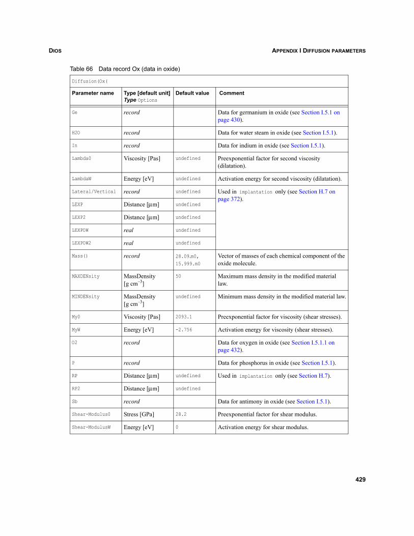
DIOS APPENDIX I DIFFUSION PARAMETERS
Ge record Data for germanium in oxide (see Section I.5.1 on page 430).
H2O record Data for water steam in oxide (see Section I.5.1).
In record Data for indium in oxide (see Section I.5.1).
Lambda0 Viscosity [Pas] undefined Preexponential factor for second viscosity (dilatation).
LambdaW Energy [eV] undefined Activation energy for second viscosity (dilatation).
Lateral/Vertical record undefined Used in implantation only (see Section H.7 on page 372).
LEXP Distance [μm] undefined
LEXP2 Distance [μm] undefined
LEXPOW real undefined
LEXPOW2 real undefined
Mass() record 28.09.m0, 15.999.m0
Vector of masses of each chemical component of the oxide molecule.
MAXDENsity MassDensity[g cm–3]
50 Maximum mass density in the modified material law.
MINDENsity MassDensity [g cm–3]
undefined Minimum mass density in the modified material law.
My0 Viscosity [Pas] 2093.1 Preexponential factor for viscosity (shear stresses).
MyW Energy [eV] -2.756 Activation energy for viscosity (shear stresses).
O2 record Data for oxygen in oxide (see Section I.5.1.1 on page 432).
P record Data for phosphorus in oxide (see Section I.5.1).
RP Distance [μm] undefined Used in implantation only (see Section H.7).
RP2 Distance [μm] undefined
Sb record Data for antimony in oxide (see Section I.5.1).
Shear-Modulus0 Stress [GPa] 28.2 Preexponential factor for shear modulus.
Shear-ModulusW Energy [eV] 0 Activation energy for shear modulus.
Table 66 Data record Ox (data in oxide)
Diffusion(Ox(
Parameter name Type [default unit]Type Options
Default value Comment
429
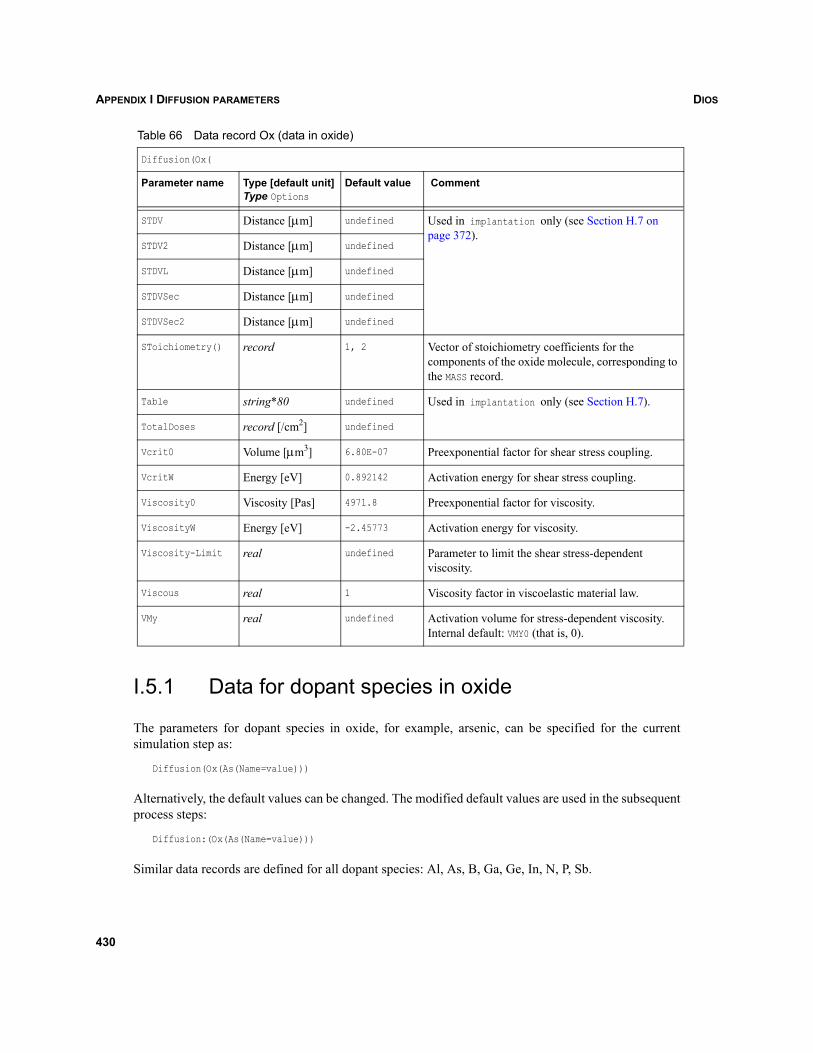
DIOSAPPENDIX I DIFFUSION PARAMETERS
I.5.1 Data for dopant species in oxide
The parameters for dopant species in oxide, for example, arsenic, can be specified for the currentsimulation step as:
Diffusion(Ox(As(Name=value)))
Alternatively, the default values can be changed. The modified default values are used in the subsequentprocess steps:
Diffusion:(Ox(As(Name=value)))
Similar data records are defined for all dopant species: Al, As, B, Ga, Ge, In, N, P, Sb.
STDV Distance [μm] undefined Used in implantation only (see Section H.7 on page 372).
STDV2 Distance [μm] undefined
STDVL Distance [μm] undefined
STDVSec Distance [μm] undefined
STDVSec2 Distance [μm] undefined
SToichiometry() record 1, 2 Vector of stoichiometry coefficients for the components of the oxide molecule, corresponding to the MASS record.
Table string*80 undefined Used in implantation only (see Section H.7).
TotalDoses record [/cm2] undefined
Vcrit0 Volume [μm3] 6.80E-07 Preexponential factor for shear stress coupling.
VcritW Energy [eV] 0.892142 Activation energy for shear stress coupling.
Viscosity0 Viscosity [Pas] 4971.8 Preexponential factor for viscosity.
ViscosityW Energy [eV] -2.45773 Activation energy for viscosity.
Viscosity-Limit real undefined Parameter to limit the shear stress-dependent viscosity.
Viscous real 1 Viscosity factor in viscoelastic material law.
VMy real undefined Activation volume for stress-dependent viscosity. Internal default: VMY0 (that is, 0).
Table 66 Data record Ox (data in oxide)
Diffusion(Ox(
Parameter name Type [default unit]Type Options
Default value Comment
430
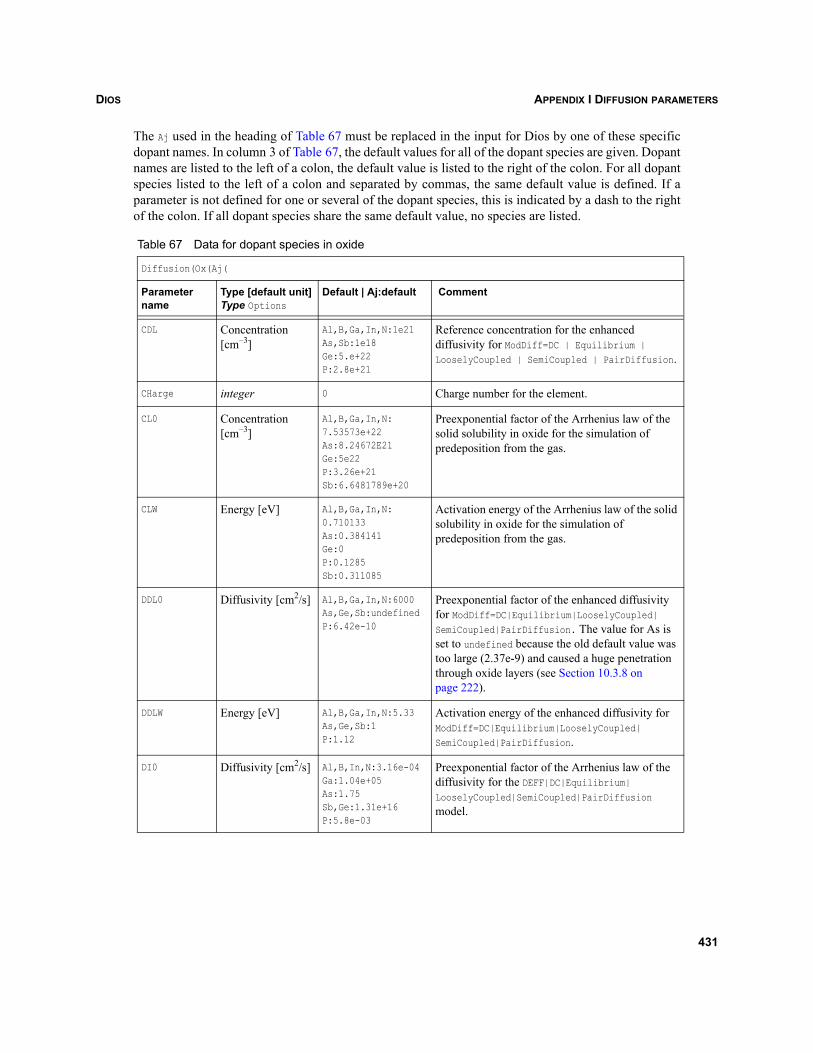
DIOS APPENDIX I DIFFUSION PARAMETERS
The Aj used in the heading of Table 67 must be replaced in the input for Dios by one of these specificdopant names. In column 3 of Table 67, the default values for all of the dopant species are given. Dopantnames are listed to the left of a colon, the default value is listed to the right of the colon. For all dopantspecies listed to the left of a colon and separated by commas, the same default value is defined. If aparameter is not defined for one or several of the dopant species, this is indicated by a dash to the rightof the colon. If all dopant species share the same default value, no species are listed.
Table 67 Data for dopant species in oxide
Diffusion(Ox(Aj(
Parameter name
Type [default unit]Type Options
Default | Aj:default Comment
CDL Concentration [cm–3]
Al,B,Ga,In,N:1e21As,Sb:1e18Ge:5.e+22P:2.8e+21
Reference concentration for the enhanced diffusivity for ModDiff=DC | Equilibrium | LooselyCoupled | SemiCoupled | PairDiffusion.
CHarge integer 0 Charge number for the element.
CL0 Concentration [cm–3]
Al,B,Ga,In,N:7.53573e+22As:8.24672E21Ge:5e22P:3.26e+21Sb:6.6481789e+20
Preexponential factor of the Arrhenius law of the solid solubility in oxide for the simulation of predeposition from the gas.
CLW Energy [eV] Al,B,Ga,In,N:0.710133As:0.384141Ge:0P:0.1285Sb:0.311085
Activation energy of the Arrhenius law of the solid solubility in oxide for the simulation of predeposition from the gas.
DDL0 Diffusivity [cm2/s] Al,B,Ga,In,N:6000As,Ge,Sb:undefinedP:6.42e-10
Preexponential factor of the enhanced diffusivity for ModDiff=DC|Equilibrium|LooselyCoupled|SemiCoupled|PairDiffusion. The value for As is set to undefined because the old default value was too large (2.37e-9) and caused a huge penetration through oxide layers (see Section 10.3.8 on page 222).
DDLW Energy [eV] Al,B,Ga,In,N:5.33As,Ge,Sb:1P:1.12
Activation energy of the enhanced diffusivity for ModDiff=DC|Equilibrium|LooselyCoupled| SemiCoupled|PairDiffusion.
DI0 Diffusivity [cm2/s] Al,B,In,N:3.16e-04Ga:1.04e+05As:1.75Sb,Ge:1.31e+16P:5.8e-03
Preexponential factor of the Arrhenius law of the diffusivity for the DEFF|DC|Equilibrium| LooselyCoupled|SemiCoupled|PairDiffusion model.
431
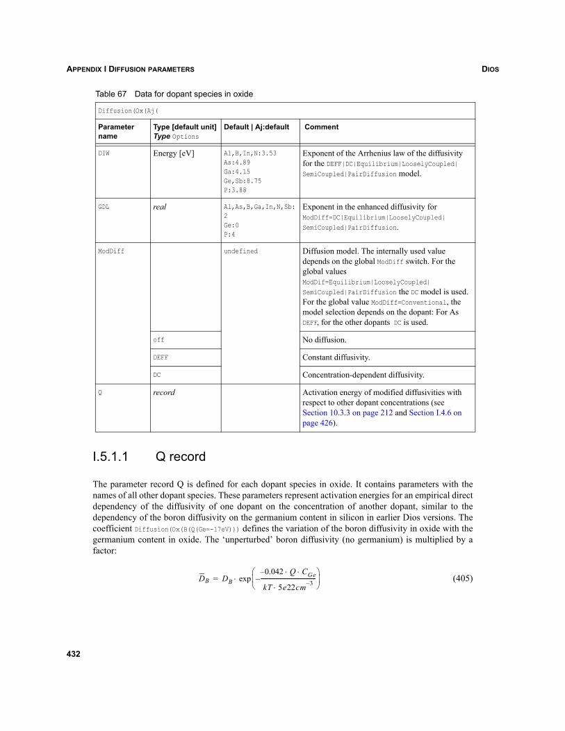
DIOSAPPENDIX I DIFFUSION PARAMETERS
I.5.1.1 Q record
The parameter record Q is defined for each dopant species in oxide. It contains parameters with thenames of all other dopant species. These parameters represent activation energies for an empirical directdependency of the diffusivity of one dopant on the concentration of another dopant, similar to thedependency of the boron diffusivity on the germanium content in silicon in earlier Dios versions. Thecoefficient Diffusion(Ox(B(Q(Ge=-17eV))) defines the variation of the boron diffusivity in oxide with thegermanium content in oxide. The ‘unperturbed’ boron diffusivity (no germanium) is multiplied by afactor:
(405)
DIW Energy [eV] Al,B,In,N:3.53As:4.89Ga:4.15Ge,Sb:8.75P:3.88
Exponent of the Arrhenius law of the diffusivity for the DEFF|DC|Equilibrium|LooselyCoupled|SemiCoupled|PairDiffusion model.
GDL real Al,As,B,Ga,In,N,Sb:2Ge:0P:4
Exponent in the enhanced diffusivity for ModDiff=DC|Equilibrium|LooselyCoupled| SemiCoupled|PairDiffusion.
ModDiff undefined Diffusion model. The internally used value depends on the global ModDiff switch. For the global values ModDif=Equilibrium|LooselyCoupled|SemiCoupled|PairDiffusion the DC model is used. For the global value ModDiff=Conventional, the model selection depends on the dopant: For As DEFF, for the other dopants DC is used.
off No diffusion.
DEFF Constant diffusivity.
DC Concentration-dependent diffusivity.
Q record Activation energy of modified diffusivities with respect to other dopant concentrations (see Section 10.3.3 on page 212 and Section I.4.6 on page 426).
Table 67 Data for dopant species in oxide
Diffusion(Ox(Aj(
Parameter name
Type [default unit]Type Options
Default | Aj:default Comment
DB DB0.042 Q C⋅ ⋅– Ge
kT 5e22cm 3–⋅----------------------------------------–
⎝ ⎠⎜ ⎟⎛ ⎞
exp⋅=
432
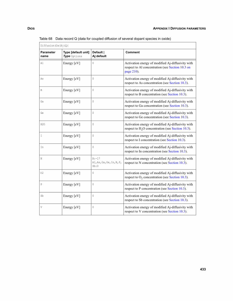
DIOS APPENDIX I DIFFUSION PARAMETERS
Table 68 Data record Q (data for coupled diffusion of several dopant species in oxide)
Diffusion(Ox(Aj(Q(
Parameter name
Type [default unit]Type Options
Default | Aj:default
Comment
Al Energy [eV] 0 Activation energy of modified Aj-diffusivity with respect to Al concentration (see Section 10.3 on page 210).
As Energy [eV] 0 Activation energy of modified Aj-diffusivity with respect to As concentration (see Section 10.3).
B Energy [eV] 0 Activation energy of modified Aj-diffusivity with respect to B concentration (see Section 10.3).
Ga Energy [eV] 0 Activation energy of modified Aj-diffusivity with respect to Ga concentration (see Section 10.3).
Ge Energy [eV] 0 Activation energy of modified Aj-diffusivity with respect to Ge concentration (see Section 10.3).
H2O Energy [eV] 0 Activation energy of modified Aj-diffusivity with respect to H2O concentration (see Section 10.3).
I Energy [eV] 0 Activation energy of modified Aj-diffusivity with respect to I concentration (see Section 10.3).
In Energy [eV] 0 Activation energy of modified Aj-diffusivity with respect to In concentration (see Section 10.3).
N Energy [eV] B:-17Al,As,Ga,Ge,In,N,P,Sb:0
Activation energy of modified Aj-diffusivity with respect to N concentration (see Section 10.3).
O2 Energy [eV] 0 Activation energy of modified Aj-diffusivity with respect to O2 concentration (see Section 10.3).
P Energy [eV] 0 Activation energy of modified Aj-diffusivity with respect to P concentration (see Section 10.3).
Sb Energy [eV] 0 Activation energy of modified Aj-diffusivity with respect to Sb concentration (see Section 10.3).
V Energy [eV] 0 Activation energy of modified Aj-diffusivity with respect to V concentration (see Section 10.3).
433
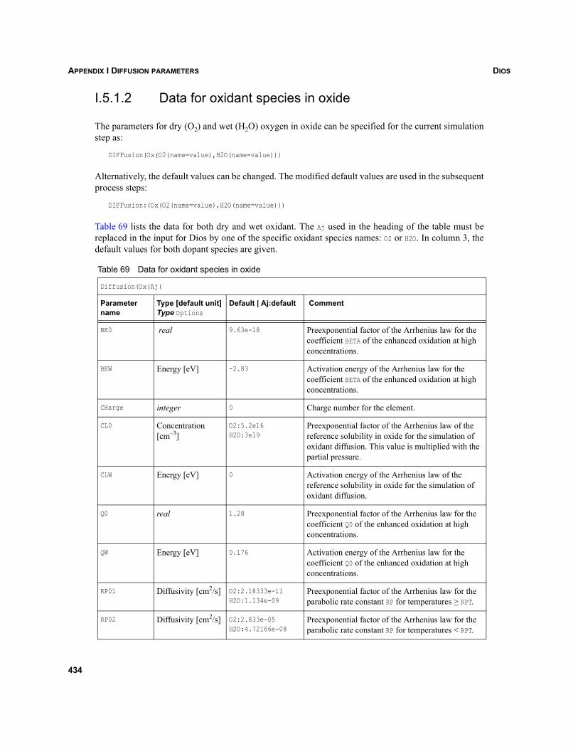
DIOSAPPENDIX I DIFFUSION PARAMETERS
I.5.1.2 Data for oxidant species in oxide
The parameters for dry (O2) and wet (H2O) oxygen in oxide can be specified for the current simulationstep as:
DIFFusion(Ox(O2(name=value),H2O(name=value)))
Alternatively, the default values can be changed. The modified default values are used in the subsequentprocess steps:
DIFFusion:(Ox(O2(name=value),H2O(name=value)))
Table 69 lists the data for both dry and wet oxidant. The Aj used in the heading of the table must bereplaced in the input for Dios by one of the specific oxidant species names: O2 or H2O. In column 3, thedefault values for both dopant species are given.
Table 69 Data for oxidant species in oxide
Diffusion(Ox(Aj(
Parameter name
Type [default unit]Type Options
Default | Aj:default Comment
BE0 real 9.63e-18 Preexponential factor of the Arrhenius law for the coefficient BETA of the enhanced oxidation at high concentrations.
BEW Energy [eV] -2.83 Activation energy of the Arrhenius law for the coefficient BETA of the enhanced oxidation at high concentrations.
CHarge integer 0 Charge number for the element.
CL0 Concentration [cm–3]
O2:5.2e16H2O:3e19
Preexponential factor of the Arrhenius law of the reference solubility in oxide for the simulation of oxidant diffusion. This value is multiplied with the partial pressure.
CLW Energy [eV] 0 Activation energy of the Arrhenius law of the reference solubility in oxide for the simulation of oxidant diffusion.
Q0 real 1.28 Preexponential factor of the Arrhenius law for the coefficient Q0 of the enhanced oxidation at high concentrations.
QW Energy [eV] 0.176 Activation energy of the Arrhenius law for the coefficient Q0 of the enhanced oxidation at high concentrations.
RP01 Diffusivity [cm2/s] O2:2.18333e-11H2O:1.134e-09
Preexponential factor of the Arrhenius law for the parabolic rate constant RP for temperatures > RPT.
RP02 Diffusivity [cm2/s] O2:2.833e-05H2O:4.72166e-08
Preexponential factor of the Arrhenius law for the parabolic rate constant RP for temperatures < RPT.
434
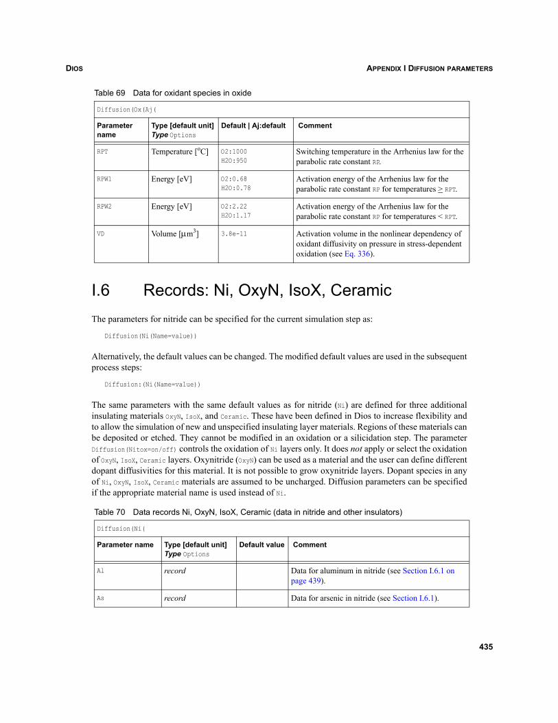
DIOS APPENDIX I DIFFUSION PARAMETERS
I.6 Records: Ni, OxyN, IsoX, CeramicThe parameters for nitride can be specified for the current simulation step as:
Diffusion(Ni(Name=value))
Alternatively, the default values can be changed. The modified default values are used in the subsequentprocess steps:
Diffusion:(Ni(Name=value))
The same parameters with the same default values as for nitride (Ni) are defined for three additionalinsulating materials OxyN, IsoX, and Ceramic. These have been defined in Dios to increase flexibility andto allow the simulation of new and unspecified insulating layer materials. Regions of these materials canbe deposited or etched. They cannot be modified in an oxidation or a silicidation step. The parameterDiffusion(Nitox=on/off) controls the oxidation of Ni layers only. It does not apply or select the oxidationof OxyN, IsoX, Ceramic layers. Oxynitride (OxyN) can be used as a material and the user can define differentdopant diffusivities for this material. It is not possible to grow oxynitride layers. Dopant species in anyof Ni, OxyN, IsoX, Ceramic materials are assumed to be uncharged. Diffusion parameters can be specifiedif the appropriate material name is used instead of Ni.
RPT Temperature [oC] O2:1000H2O:950
Switching temperature in the Arrhenius law for the parabolic rate constant RP.
RPW1 Energy [eV] O2:0.68H2O:0.78
Activation energy of the Arrhenius law for the parabolic rate constant RP for temperatures > RPT.
RPW2 Energy [eV] O2:2.22H2O:1.17
Activation energy of the Arrhenius law for the parabolic rate constant RP for temperatures < RPT.
VD Volume [μm3] 3.8e-11 Activation volume in the nonlinear dependency of oxidant diffusivity on pressure in stress-dependent oxidation (see Eq. 336).
Table 70 Data records Ni, OxyN, IsoX, Ceramic (data in nitride and other insulators)
Diffusion(Ni(
Parameter name Type [default unit]Type Options
Default value Comment
Al record Data for aluminum in nitride (see Section I.6.1 on page 439).
As record Data for arsenic in nitride (see Section I.6.1).
Table 69 Data for oxidant species in oxide
Diffusion(Ox(Aj(
Parameter name
Type [default unit]Type Options
Default | Aj:default Comment
435
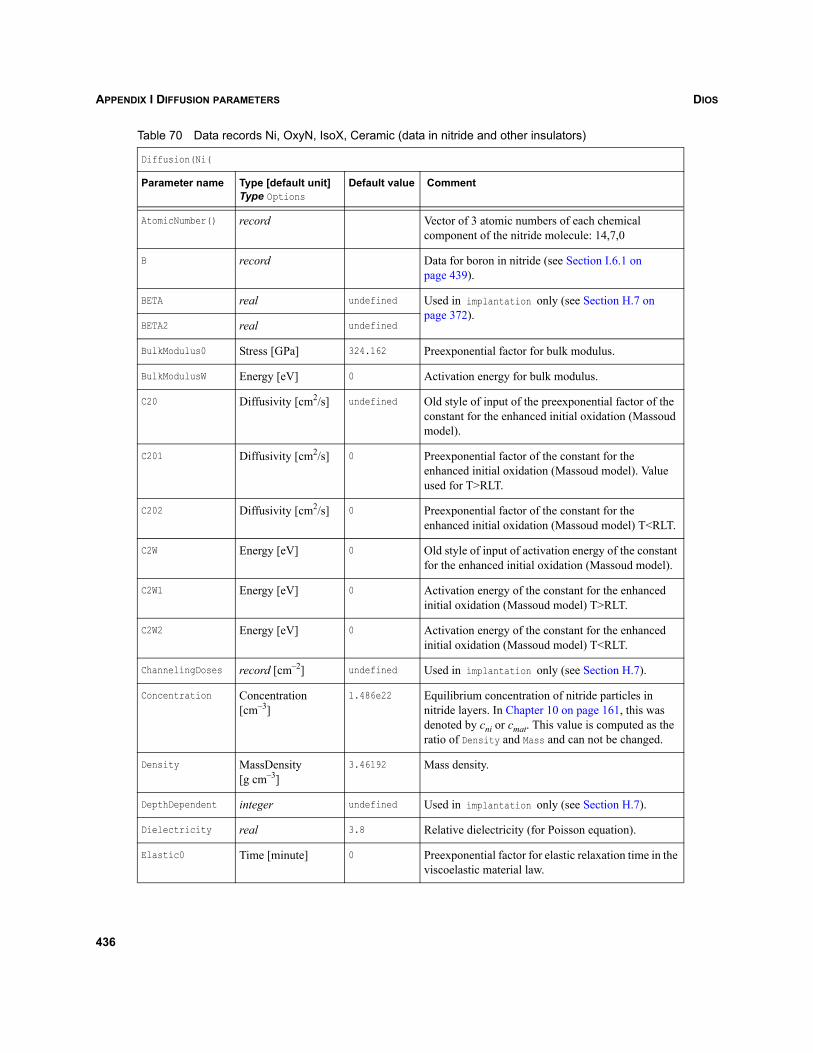
DIOSAPPENDIX I DIFFUSION PARAMETERS
AtomicNumber() record Vector of 3 atomic numbers of each chemical component of the nitride molecule: 14,7,0
B record Data for boron in nitride (see Section I.6.1 on page 439).
BETA real undefined Used in implantation only (see Section H.7 on page 372).
BETA2 real undefined
BulkModulus0 Stress [GPa] 324.162 Preexponential factor for bulk modulus.
BulkModulusW Energy [eV] 0 Activation energy for bulk modulus.
C20 Diffusivity [cm2/s] undefined Old style of input of the preexponential factor of the constant for the enhanced initial oxidation (Massoud model).
C201 Diffusivity [cm2/s] 0 Preexponential factor of the constant for the enhanced initial oxidation (Massoud model). Value used for T>RLT.
C202 Diffusivity [cm2/s] 0 Preexponential factor of the constant for the enhanced initial oxidation (Massoud model) T<RLT.
C2W Energy [eV] 0 Old style of input of activation energy of the constant for the enhanced initial oxidation (Massoud model).
C2W1 Energy [eV] 0 Activation energy of the constant for the enhanced initial oxidation (Massoud model) T>RLT.
C2W2 Energy [eV] 0 Activation energy of the constant for the enhanced initial oxidation (Massoud model) T<RLT.
ChannelingDoses record [cm–2] undefined Used in implantation only (see Section H.7).
Concentration Concentration [cm–3]
1.486e22 Equilibrium concentration of nitride particles in nitride layers. In Chapter 10 on page 161, this was denoted by cni or cmat. This value is computed as the ratio of Density and Mass and can not be changed.
Density MassDensity [g cm–3]
3.46192 Mass density.
DepthDependent integer undefined Used in implantation only (see Section H.7).
Dielectricity real 3.8 Relative dielectricity (for Poisson equation).
Elastic0 Time [minute] 0 Preexponential factor for elastic relaxation time in the viscoelastic material law.
Table 70 Data records Ni, OxyN, IsoX, Ceramic (data in nitride and other insulators)
Diffusion(Ni(
Parameter name Type [default unit]Type Options
Default value Comment
436
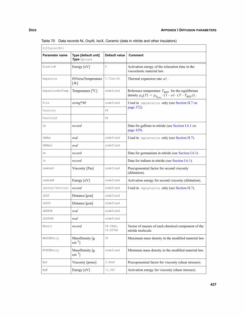
DIOS APPENDIX I DIFFUSION PARAMETERS
ElasticW Energy [eV] 0 Activation energy of the relaxation time in the viscoelastic material law.
Expansion INVerseTemperature [/K]
7.732e-06 Thermal expansion rate .
ExpansionRefTemp Temperature [oC] undefined Reference temperature for the equilibrium density .
File string*80 undefined Used in implantation only (see Section H.7 on page 372).
Function P4
Function2 P4
Ga record Data for gallium in nitride (see Section I.6.1 on page 439).
GAMma real undefined Used in implantation only (see Section H.7).
GAMma2 real undefined
Ge record Data for germanium in nitride (see Section I.6.1).
In record Data for indium in nitride (see Section I.6.1).
Lambda0 Viscosity [Pas] undefined Preexponential factor for second viscosity (dilatation).
LambdaW Energy [eV] undefined Activation energy for second viscosity (dilatation).
Lateral/Vertical record undefined Used in implantation only (see Section H.7).
LEXP Distance [μm] undefined
LEXP2 Distance [μm] undefined
LEXPOW real undefined
LEXPOW2 real undefined
Mass() record 28.09m0,14.007m0
Vector of masses of each chemical component of the nitride molecule.
MAXDENsity MassDensity [g cm–3]
50 Maximum mass density in the modified material law.
MINDENsity MassDensity [g cm–3]
undefined Minimum mass density in the modified material law.
My0 Viscosity [poise] 3.94e9 Preexponential factor for viscosity (shear stresses).
MyW Energy [eV] -1.365 Activation energy for viscosity (shear stresses).
Table 70 Data records Ni, OxyN, IsoX, Ceramic (data in nitride and other insulators)
Diffusion(Ni(
Parameter name Type [default unit]Type Options
Default value Comment
a1
TREFρ0 T( ) ρ0REF
1 a1 T TREF–( )⋅–( )⋅=
437
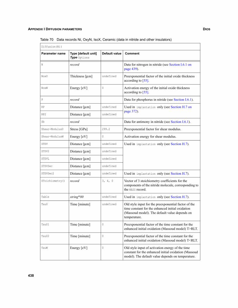
DIOSAPPENDIX I DIFFUSION PARAMETERS
N record Data for nitrogen in nitride (see Section I.6.1 on page 439).
Nox0 Thickness [μm] undefined Preexponential factor of the initial oxide thickness according to [55].
NoxW Energy [eV] 0 Activation energy of the initial oxide thickness according to [55].
P record Data for phosphorus in nitride (see Section I.6.1).
RP Distance [μm] undefined Used in implantation only (see Section H.7 on page 372).
RP2 Distance [μm] undefined
Sb record Data for antimony in nitride (see Section I.6.1).
Shear-Modulus0 Stress [GPa] 299.2 Preexponential factor for shear modulus.
Shear-ModulusW Energy [eV] 0 Activation energy for shear modulus.
STDV Distance [μm] undefined Used in implantation only (see Section H.7).
STDV2 Distance [μm] undefined
STDVL Distance [μm] undefined
STDVSec Distance [μm] undefined
STDVSec2 Distance [μm] undefined Used in implantation only (see Section H.7).
SToichiometry() record 3, 4, 0 Vector of 3 stoichiometry coefficients for the components of the nitride molecule, corresponding to the MASS record.
Table string*80 undefined Used in implantation only (see Section H.7).
Tau0 Time [minute] undefined Old style input for the preexponential factor of the time constant for the enhanced initial oxidation (Massoud model). The default value depends on temperature.
Tau01 Time [minute] 0 Preexponential factor of the time constant for the enhanced initial oxidation (Massoud model) T>RLT.
Tau02 Time [minute] 0 Preexponential factor of the time constant for the enhanced initial oxidation (Massoud model) T<RLT.
TauW Energy [eV] 0 Old style input of activation energy of the time constant for the enhanced initial oxidation (Massoud model). The default value depends on temperature.
Table 70 Data records Ni, OxyN, IsoX, Ceramic (data in nitride and other insulators)
Diffusion(Ni(
Parameter name Type [default unit]Type Options
Default value Comment
438
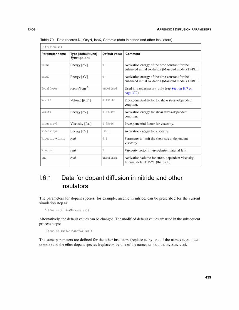
DIOS APPENDIX I DIFFUSION PARAMETERS
I.6.1 Data for dopant diffusion in nitride and other insulators
The parameters for dopant species, for example, arsenic in nitride, can be prescribed for the currentsimulation step as:
Diffusion(Ni(As(Name=value)))
Alternatively, the default values can be changed. The modified default values are used in the subsequentprocess steps:
Diffusion:(Ni(As(Name=value)))
The same parameters are defined for the other insulators (replace Ni by one of the names OxyN, IsoX,Ceramic) and the other dopant species (replace Aj by one of the names Al,As,B,Ga,Ge,In,N,P,Sb).
TauW1 Energy [eV] 0 Activation energy of the time constant for the enhanced initial oxidation (Massoud model) T>RLT.
TauW2 Energy [eV] 0 Activation energy of the time constant for the enhanced initial oxidation (Massoud model) T<RLT.
TotalDoses record [cm–2] undefined Used in implantation only (see Section H.7 on page 372).
Vcrit0 Volume [μm3] 9.19E-08 Preexponential factor for shear stress-dependent coupling.
VcritW Energy [eV] 0.697898 Activation energy for shear stress-dependent coupling.
viscosity0 Viscosity [Pas] 4.75E06 Preexponential factor for viscosity.
ViscosityW Energy [eV] -2.15 Activation energy for viscosity.
Viscosity-Limit real 0.1 Parameter to limit the shear stress-dependent viscosity.
Viscous real 1 Viscosity factor in viscoelastic material law.
VMy real undefined Activation volume for stress-dependent viscosity. Internal default: VMY0 (that is, 0).
Table 70 Data records Ni, OxyN, IsoX, Ceramic (data in nitride and other insulators)
Diffusion(Ni(
Parameter name Type [default unit]Type Options
Default value Comment
439
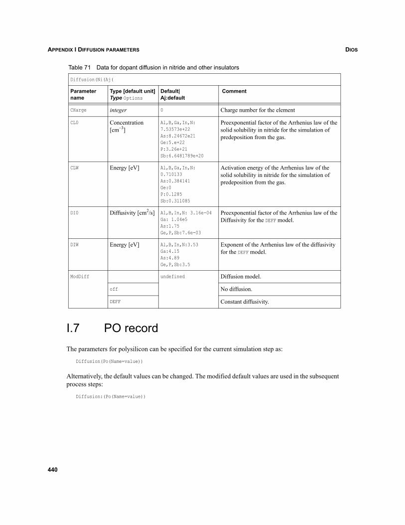
DIOSAPPENDIX I DIFFUSION PARAMETERS
I.7 PO recordThe parameters for polysilicon can be specified for the current simulation step as:
Diffusion(Po(Name=value))
Alternatively, the default values can be changed. The modified default values are used in the subsequentprocess steps:
Diffusion:(Po(Name=value))
Table 71 Data for dopant diffusion in nitride and other insulators
Diffusion(Ni(Aj(
Parameter name
Type [default unit]Type Options
Default|Aj:default
Comment
CHarge integer 0 Charge number for the element
CL0 Concentration [cm–3]
Al,B,Ga,In,N:7.53573e+22As:8.24672e21Ge:5.e+22P:3.26e+21Sb:6.6481789e+20
Preexponential factor of the Arrhenius law of the solid solubility in nitride for the simulation of predeposition from the gas.
CLW Energy [eV] Al,B,Ga,In,N:0.710133As:0.384141Ge:0P:0.1285Sb:0.311085
Activation energy of the Arrhenius law of the solid solubility in nitride for the simulation of predeposition from the gas.
DI0 Diffusivity [cm2/s] Al,B,In,N: 3.16e-04Ga: 1.04e5As:1.75Ge,P,Sb:7.6e-03
Preexponential factor of the Arrhenius law of the Diffusivity for the DEFF model.
DIW Energy [eV] Al,B,In,N:3.53Ga:4.15As:4.89Ge,P,Sb:3.5
Exponent of the Arrhenius law of the diffusivity for the DEFF model.
ModDiff undefined Diffusion model.
off No diffusion.
DEFF Constant diffusivity.
440
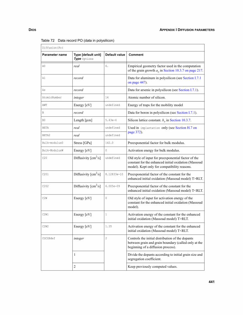
DIOS APPENDIX I DIFFUSION PARAMETERS
Table 72 Data record PO (data in polysilicon)
Diffusion(Po(
Parameter name Type [default unit]Type Options
Default value Comment
A0 real 6. Empirical geometry factor used in the computation of the grain growth ao in Section 10.3.7 on page 217.
Al record Data for aluminum in polysilicon (see Section I.7.1 on page 447).
As record Data for arsenic in polysilicon (see Section I.7.1).
AtomicNumber integer 14 Atomic number of silicon.
AWT Energy [eV] undefined Energy of traps for the mobility model
B record Data for boron in polysilicon (see Section I.7.1).
B0 Length [μm] 5.43e-4 Silicon lattice constant. bo in Section 10.3.7.
BETA real undefined Used in implantation only (see Section H.7 on page 372).
BETA2 real undefined
Bulk-modulus0 Stress [GPa] 142.0 Preexponential factor for bulk modulus.
Bulk-ModulusW Energy [eV] 0 Activation energy for bulk modulus.
C20 Diffusivity [cm2/s] undefined Old style of input for preexponential factor of the constant for the enhanced initial oxidation (Massoud model). Kept only for compatibility reasons.
C201 Diffusivity [cm2/s] 8.12833e-10 Preexponential factor of the constant for the enhanced initial oxidation (Massoud model) T>RLT.
C202 Diffusivity [cm2/s] 6.005e-09 Preexponential factor of the constant for the enhanced initial oxidation (Massoud model) T<RLT.
C2W Energy [eV] 0 Old style of input for activation energy of the constant for the enhanced initial oxidation (Massoud model).
C2W1 Energy [eV] 1 Activation energy of the constant for the enhanced initial oxidation (Massoud model) T>RLT.
C2W2 Energy [eV] 1.35 Activation energy of the constant for the enhanced initial oxidation (Massoud model) T<RLT.
CGCGBdef integer 2 Controls the initial distribution of the dopants between grain and grain boundary (called only at the beginning of a diffusion process).
1 Divide the dopants according to initial grain size and segregation coefficient.
2 Keep previously computed values.
441
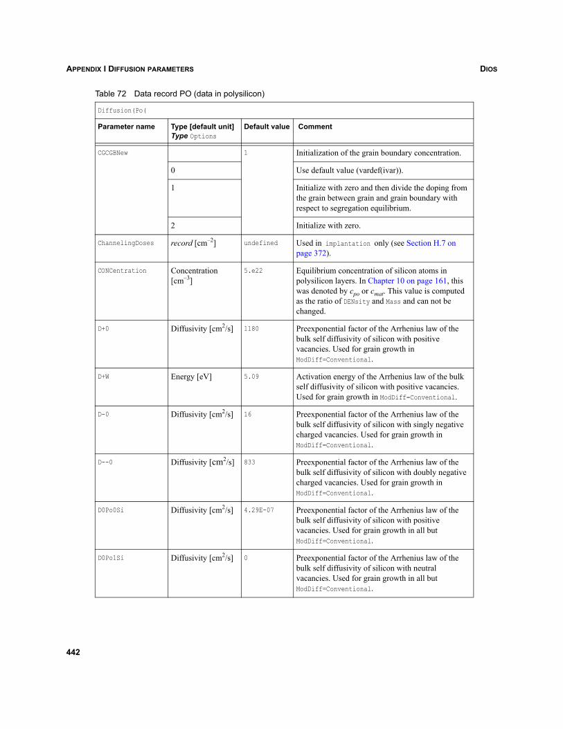
DIOSAPPENDIX I DIFFUSION PARAMETERS
CGCGBNew 1 Initialization of the grain boundary concentration.
0 Use default value (vardef(ivar)).
1 Initialize with zero and then divide the doping from the grain between grain and grain boundary with respect to segregation equilibrium.
2 Initialize with zero.
ChannelingDoses record [cm–2] undefined Used in implantation only (see Section H.7 on page 372).
CONCentration Concentration [cm–3]
5.e22 Equilibrium concentration of silicon atoms in polysilicon layers. In Chapter 10 on page 161, this was denoted by cpo or cmat. This value is computed as the ratio of DENsity and Mass and can not be changed.
D+0 Diffusivity [cm2/s] 1180 Preexponential factor of the Arrhenius law of the bulk self diffusivity of silicon with positive vacancies. Used for grain growth in ModDiff=Conventional.
D+W Energy [eV] 5.09 Activation energy of the Arrhenius law of the bulk self diffusivity of silicon with positive vacancies. Used for grain growth in ModDiff=Conventional.
D-0 Diffusivity [cm2/s] 16 Preexponential factor of the Arrhenius law of the bulk self diffusivity of silicon with singly negative charged vacancies. Used for grain growth in ModDiff=Conventional.
D--0 Diffusivity [cm2/s] 833 Preexponential factor of the Arrhenius law of the bulk self diffusivity of silicon with doubly negative charged vacancies. Used for grain growth in ModDiff=Conventional.
D0Po0Si Diffusivity [cm2/s] 4.29E-07 Preexponential factor of the Arrhenius law of the bulk self diffusivity of silicon with positive vacancies. Used for grain growth in all but ModDiff=Conventional.
D0Po1Si Diffusivity [cm2/s] 0 Preexponential factor of the Arrhenius law of the bulk self diffusivity of silicon with neutral vacancies. Used for grain growth in all but ModDiff=Conventional.
Table 72 Data record PO (data in polysilicon)
Diffusion(Po(
Parameter name Type [default unit]Type Options
Default value Comment
442
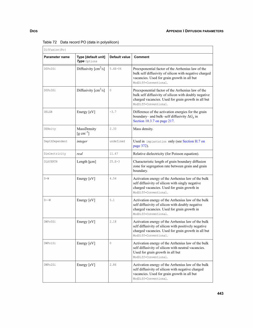
DIOS APPENDIX I DIFFUSION PARAMETERS
D0Po2Si Diffusivity [cm2/s] 5.6E-06 Preexponential factor of the Arrhenius law of the bulk self diffusivity of silicon with negative charged vacancies. Used for grain growth in all but ModDiff=Conventional.
D0Po3Si Diffusivity [cm2/s] 0 Preexponential factor of the Arrhenius law of the bulk self diffusivity of silicon with doubly negative charged vacancies. Used for grain growth in all but ModDiff=Conventional.
DELGB Energy [eV] -3.7 Difference of the activation energies for the grain boundary– and bulk–self diffusivity ΔGb in Section 10.3.7 on page 217.
DENsity MassDensity [g cm–3]
2.33 Mass density.
DepthDependent integer undefined Used in implantation only (see Section H.7 on page 372).
Dielectricity real 11.67 Relative dielectricity (for Poisson equation).
DLAYERTH Length [μm] 25.E-3 Characteristic length of grain boundary diffusion zone for segregation rate between grain and grain boundary.
D-W Energy [eV] 4.54 Activation energy of the Arrhenius law of the bulk self diffusivity of silicon with singly negative charged vacancies. Used for grain growth in ModDiff=Conventional.
D--W Energy [eV] 5.1 Activation energy of the Arrhenius law of the bulk self diffusivity of silicon with doubly negative charged vacancies. Used for grain growth in ModDiff=Conventional.
DWPo0Si Energy [eV] 2.18 Activation energy of the Arrhenius law of the bulk self diffusivity of silicon with positively negative charged vacancies. Used for grain growth in all but ModDiff=Conventional.
DWPo1Si Energy [eV] 0 Activation energy of the Arrhenius law of the bulk self diffusivity of silicon with neutral vacancies. Used for grain growth in all but ModDiff=Conventional.
DWPo2Si Energy [eV] 2.86 Activation energy of the Arrhenius law of the bulk self diffusivity of silicon with negative charged vacancies. Used for grain growth in all but ModDiff=Conventional.
Table 72 Data record PO (data in polysilicon)
Diffusion(Po(
Parameter name Type [default unit]Type Options
Default value Comment
443
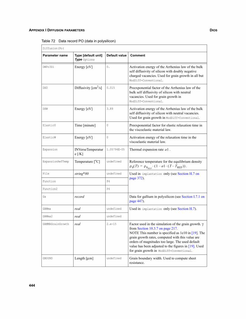
DIOSAPPENDIX I DIFFUSION PARAMETERS
DWPo3Si Energy [eV] 0. Activation energy of the Arrhenius law of the bulk self diffusivity of silicon with doubly negative charged vacancies. Used for grain growth in all but ModDiff=Conventional.
DX0 Diffusivity [cm2/s] 0.015 Preexponential factor of the Arrhenius law of the bulk self diffusivity of silicon with neutral vacancies. Used for grain growth in ModDiff=Conventional.
DXW Energy [eV] 3.89 Activation energy of the Arrhenius law of the bulk self diffusivity of silicon with neutral vacancies. Used for grain growth in ModDiff=Conventional.
Elastic0 Time [minute] 0 Preexponential factor for elastic relaxation time in the viscoelastic material law.
ElasticW Energy [eV] 0 Activation energy of the relaxation time in the viscoelastic material law.
Expansion INVerseTemperature [/K]
1.05794E-05 Thermal expansion rate .
ExpansionRefTemp Temperature [oC] undefined Reference temperature for the equilibrium density .
File string*80 undefined Used in implantation only (see Section H.7 on page 372).
Function P4
Function2 P4
Ga record Data for gallium in polysilicon (see Section I.7.1 on page 447).
GAMma real undefined Used in implantation only (see Section H.7).
GAMma2 real undefined
GAMMAGrainGrowth real 2.e-15 Factor used in the simulation of the grain growth. γ from Section 10.3.7 on page 217.NOTE This number is specified as 1e10 in [19]. The grain growth rates, computed with this value are orders of magnitudes too large. The used default value has been adjusted to the figures in [19]. Used for grain growth in ModDiff=Conventional.
GBOUND Length [μm] undefined Grain boundary width. Used to compute sheet resistance.
Table 72 Data record PO (data in polysilicon)
Diffusion(Po(
Parameter name Type [default unit]Type Options
Default value Comment
a1
ρ0 T( ) ρ0REF1 a1 T TREF–( )⋅–( )⋅=
444
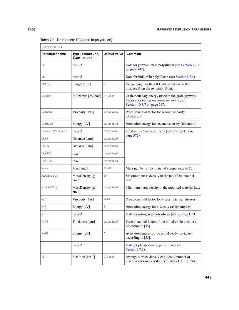
DIOS APPENDIX I DIFFUSION PARAMETERS
Ge record Data for germanium in polysilicon (see Section I.7.1 on page 447).
In record Data for indium in polysilicon (see Section I.7.1).
INTlen Length [μm] 1.0 Decay length of the OED diffusivity with the distance from the oxidation front.
LAMBDA SuEnDens [eV/cm2] 6.25e14 Grain boundary energy (used in the grain growth). Energy per unit grain boundary area λ0 in Section 10.3.7 on page 217.
Lambda0 Viscosity [Pas] undefined Preexponential factor for second viscosity (dilatation).
LambdaW Energy [eV] undefined Activation energy for second viscosity (dilatation).
Lateral/Vertical record undefined Used in implantation only (see Section H.7 on page 372).
LEXP Distance [μm] undefined
LEXP2 Distance [μm] undefined
LEXPOW real undefined
LEXPOW2 real undefined
Mass Mass [m0] 28.09 Mass number of the material components of Po.
MAXDENsity MassDensity [g cm–3]
50 Maximum mass density in the modified material law.
MINDENsity MassDensity [g cm–3]
undefined Minimum mass density in the modified material law.
My0 Viscosity [Pas] 1e14 Preexponential factor for viscosity (shear stresses).
MyW Energy [eV] 0 Activation energy for viscosity (shear stresses).
N record Data for nitrogen in polysilicon (see Section I.7.1).
Nox0 Thickness [μm] undefined Preexponential factor of the initial oxide thickness according to [55].
NoxW Energy [eV] 0. Activation energy of the initial oxide thickness according to [55].
P record Data for phosphorus in polysilicon (see Section I.7.1).
QS SurConc [cm–2] 2.64e15 Average surface density of silicon (number of reaction sites in a crystalline plane) Qs in Eq. 244.
Table 72 Data record PO (data in polysilicon)
Diffusion(Po(
Parameter name Type [default unit]Type Options
Default value Comment
445
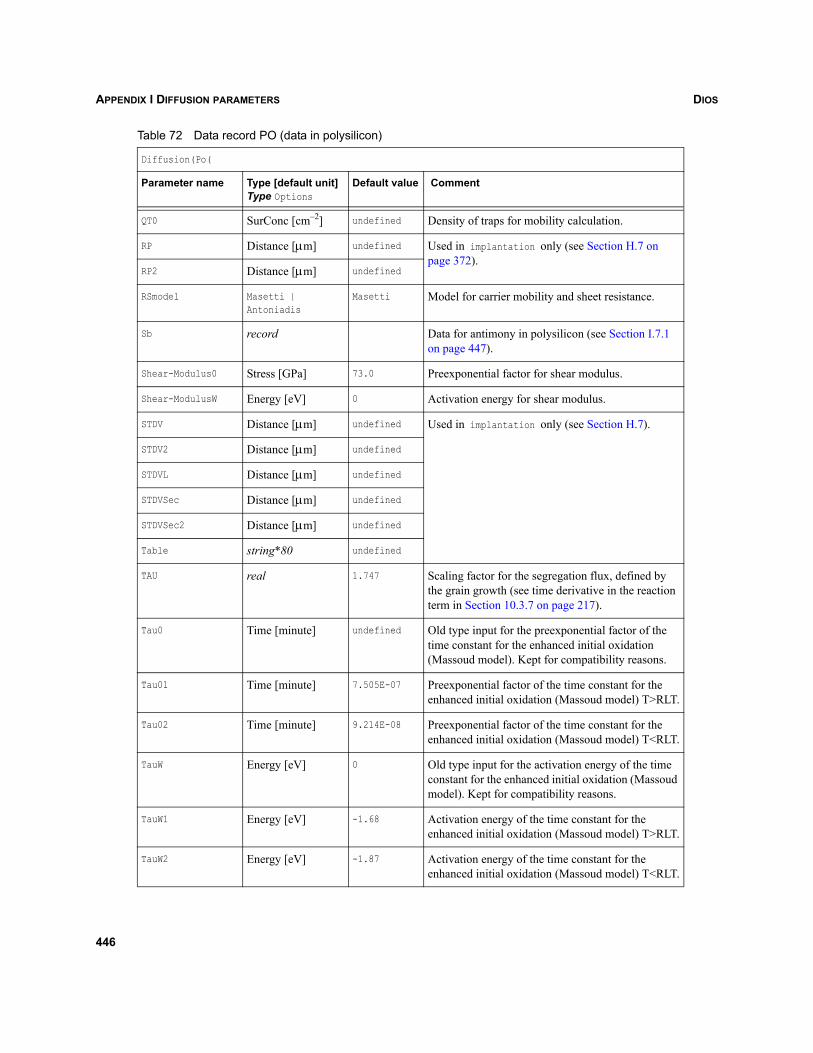
DIOSAPPENDIX I DIFFUSION PARAMETERS
QT0 SurConc [cm–2] undefined Density of traps for mobility calculation.
RP Distance [μm] undefined Used in implantation only (see Section H.7 on page 372).
RP2 Distance [μm] undefined
RSmodel Masetti | Antoniadis
Masetti Model for carrier mobility and sheet resistance.
Sb record Data for antimony in polysilicon (see Section I.7.1 on page 447).
Shear-Modulus0 Stress [GPa] 73.0 Preexponential factor for shear modulus.
Shear-ModulusW Energy [eV] 0 Activation energy for shear modulus.
STDV Distance [μm] undefined Used in implantation only (see Section H.7).
STDV2 Distance [μm] undefined
STDVL Distance [μm] undefined
STDVSec Distance [μm] undefined
STDVSec2 Distance [μm] undefined
Table string*80 undefined
TAU real 1.747 Scaling factor for the segregation flux, defined by the grain growth (see time derivative in the reaction term in Section 10.3.7 on page 217).
Tau0 Time [minute] undefined Old type input for the preexponential factor of the time constant for the enhanced initial oxidation (Massoud model). Kept for compatibility reasons.
Tau01 Time [minute] 7.505E-07 Preexponential factor of the time constant for the enhanced initial oxidation (Massoud model) T>RLT.
Tau02 Time [minute] 9.214E-08 Preexponential factor of the time constant for the enhanced initial oxidation (Massoud model) T<RLT.
TauW Energy [eV] 0 Old type input for the activation energy of the time constant for the enhanced initial oxidation (Massoud model). Kept for compatibility reasons.
TauW1 Energy [eV] -1.68 Activation energy of the time constant for the enhanced initial oxidation (Massoud model) T>RLT.
TauW2 Energy [eV] -1.87 Activation energy of the time constant for the enhanced initial oxidation (Massoud model) T<RLT.
Table 72 Data record PO (data in polysilicon)
Diffusion(Po(
Parameter name Type [default unit]Type Options
Default value Comment
446
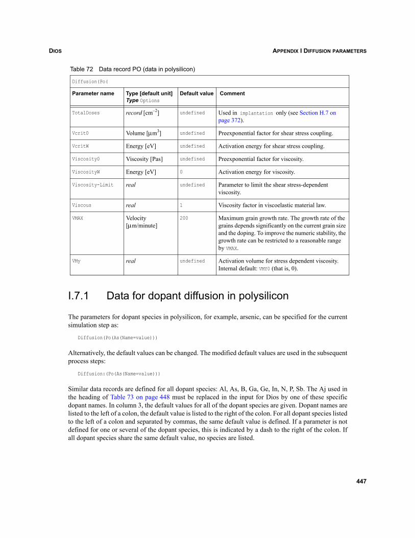
DIOS APPENDIX I DIFFUSION PARAMETERS
I.7.1 Data for dopant diffusion in polysilicon
The parameters for dopant species in polysilicon, for example, arsenic, can be specified for the currentsimulation step as:
Diffusion(Po(As(Name=value)))
Alternatively, the default values can be changed. The modified default values are used in the subsequentprocess steps:
Diffusion:(Po(As(Name=value)))
Similar data records are defined for all dopant species: Al, As, B, Ga, Ge, In, N, P, Sb. The Aj used inthe heading of Table 73 on page 448 must be replaced in the input for Dios by one of these specificdopant names. In column 3, the default values for all of the dopant species are given. Dopant names arelisted to the left of a colon, the default value is listed to the right of the colon. For all dopant species listedto the left of a colon and separated by commas, the same default value is defined. If a parameter is notdefined for one or several of the dopant species, this is indicated by a dash to the right of the colon. Ifall dopant species share the same default value, no species are listed.
TotalDoses record [cm–2] undefined Used in implantation only (see Section H.7 on page 372).
Vcrit0 Volume [μm3] undefined Preexponential factor for shear stress coupling.
VcritW Energy [eV] undefined Activation energy for shear stress coupling.
Viscosity0 Viscosity [Pas] undefined Preexponential factor for viscosity.
ViscosityW Energy [eV] 0 Activation energy for viscosity.
Viscosity-Limit real undefined Parameter to limit the shear stress-dependent viscosity.
Viscous real 1 Viscosity factor in viscoelastic material law.
VMAX Velocity[μm/minute]
200 Maximum grain growth rate. The growth rate of the grains depends significantly on the current grain size and the doping. To improve the numeric stability, the growth rate can be restricted to a reasonable range by VMAX.
VMy real undefined Activation volume for stress dependent viscosity. Internal default: VMY0 (that is, 0).
Table 72 Data record PO (data in polysilicon)
Diffusion(Po(
Parameter name Type [default unit]Type Options
Default value Comment
447
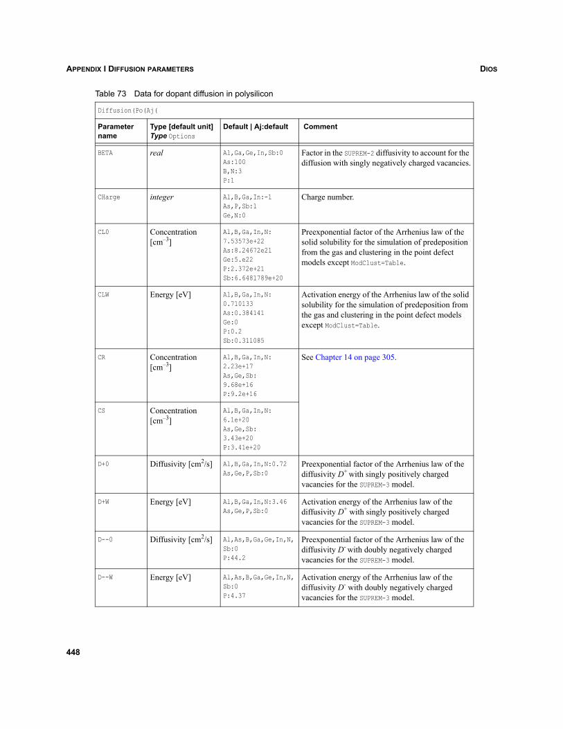
DIOSAPPENDIX I DIFFUSION PARAMETERS
Table 73 Data for dopant diffusion in polysilicon
Diffusion(Po(Aj(
Parameter name
Type [default unit]Type Options
Default | Aj:default Comment
BETA real Al,Ga,Ge,In,Sb:0As:100B,N:3P:1
Factor in the SUPREM-2 diffusivity to account for the diffusion with singly negatively charged vacancies.
CHarge integer Al,B,Ga,In:-1As,P,Sb:1Ge,N:0
Charge number.
CL0 Concentration [cm–3]
Al,B,Ga,In,N:7.53573e+22As:8.24672e21Ge:5.e22P:2.372e+21Sb:6.6481789e+20
Preexponential factor of the Arrhenius law of the solid solubility for the simulation of predeposition from the gas and clustering in the point defect models except ModClust=Table.
CLW Energy [eV] Al,B,Ga,In,N:0.710133As:0.384141Ge:0P:0.2Sb:0.311085
Activation energy of the Arrhenius law of the solid solubility for the simulation of predeposition from the gas and clustering in the point defect models except ModClust=Table.
CR Concentration [cm–3]
Al,B,Ga,In,N:2.23e+17As,Ge,Sb:9.68e+16P:9.2e+16
See Chapter 14 on page 305.
CS Concentration [cm–3]
Al,B,Ga,In,N:6.1e+20As,Ge,Sb:3.43e+20P:3.41e+20
D+0 Diffusivity [cm2/s] Al,B,Ga,In,N:0.72As,Ge,P,Sb:0
Preexponential factor of the Arrhenius law of the diffusivity D+ with singly positively charged vacancies for the SUPREM-3 model.
D+W Energy [eV] Al,B,Ga,In,N:3.46As,Ge,P,Sb:0
Activation energy of the Arrhenius law of the diffusivity D+ with singly positively charged vacancies for the SUPREM-3 model.
D--0 Diffusivity [cm2/s] Al,As,B,Ga,Ge,In,N,Sb:0P:44.2
Preexponential factor of the Arrhenius law of the diffusivity D- with doubly negatively charged vacancies for the SUPREM-3 model.
D--W Energy [eV] Al,As,B,Ga,Ge,In,N,Sb:0P:4.37
Activation energy of the Arrhenius law of the diffusivity D- with doubly negatively charged vacancies for the SUPREM-3 model.
448
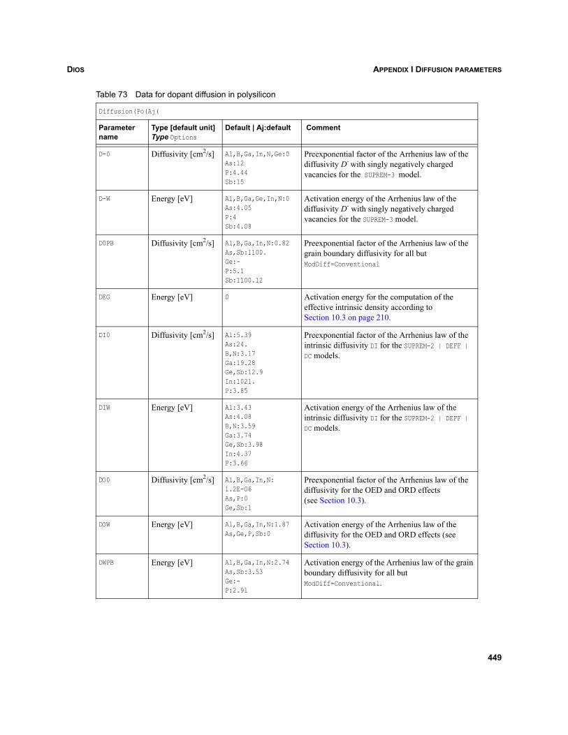
DIOS APPENDIX I DIFFUSION PARAMETERS
D-0 Diffusivity [cm2/s] Al,B,Ga,In,N,Ge:0As:12 P:4.44Sb:15
Preexponential factor of the Arrhenius law of the diffusivity D- with singly negatively charged vacancies for the SUPREM-3 model.
D-W Energy [eV] Al,B,Ga,Ge,In,N:0As:4.05P:4Sb:4.08
Activation energy of the Arrhenius law of the diffusivity D- with singly negatively charged vacancies for the SUPREM-3 model.
D0PB Diffusivity [cm2/s] Al,B,Ga,In,N:0.82As,Sb:1100.Ge:-P:5.1Sb:1100.12
Preexponential factor of the Arrhenius law of the grain boundary diffusivity for all but ModDiff=Conventional
DEG Energy [eV] 0 Activation energy for the computation of the effective intrinsic density according to Section 10.3 on page 210.
DI0 Diffusivity [cm2/s] Al:5.39As:24.B,N:3.17Ga:19.28Ge,Sb:12.9In:1021.P:3.85
Preexponential factor of the Arrhenius law of the intrinsic diffusivity DI for the SUPREM-2 | DEFF | DC models.
DIW Energy [eV] Al:3.43As:4.08B,N:3.59Ga:3.74Ge,Sb:3.98In:4.37P:3.66
Activation energy of the Arrhenius law of the intrinsic diffusivity DI for the SUPREM-2 | DEFF | DC models.
DO0 Diffusivity [cm2/s] Al,B,Ga,In,N:1.2E-06As,P:0Ge,Sb:1
Preexponential factor of the Arrhenius law of the diffusivity for the OED and ORD effects (see Section 10.3).
DOW Energy [eV] Al,B,Ga,In,N:1.87As,Ge,P,Sb:0
Activation energy of the Arrhenius law of the diffusivity for the OED and ORD effects (see Section 10.3).
DWPB Energy [eV] Al,B,Ga,In,N:2.74As,Sb:3.53Ge:-P:2.91
Activation energy of the Arrhenius law of the grain boundary diffusivity for all but ModDiff=Conventional.
Table 73 Data for dopant diffusion in polysilicon
Diffusion(Po(Aj(
Parameter name
Type [default unit]Type Options
Default | Aj:default Comment
449
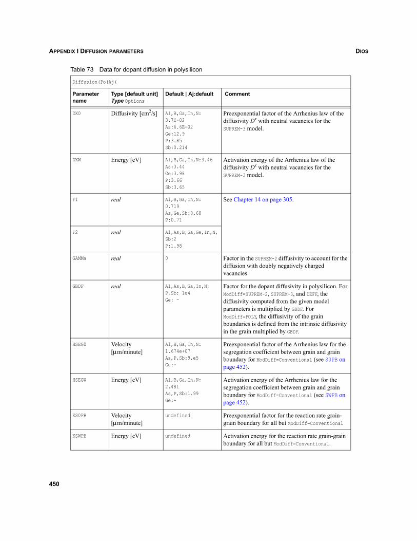
DIOSAPPENDIX I DIFFUSION PARAMETERS
DX0 Diffusivity [cm2/s] Al,B,Ga,In,N:3.7E-02As:6.6E-02Ge:12.9P:3.85Sb:0.214
Preexponential factor of the Arrhenius law of the diffusivity Dx with neutral vacancies for the SUPREM-3 model.
DXW Energy [eV] Al,B,Ga,In,N:3.46As:3.44Ge:3.98P:3.66Sb:3.65
Activation energy of the Arrhenius law of the diffusivity Dx with neutral vacancies for the SUPREM-3 model.
F1 real Al,B,Ga,In,N:0.719As,Ge,Sb:0.68P:0.71
See Chapter 14 on page 305.
F2 real Al,As,B,Ga,Ge,In,N,Sb:2P:1.98
GAMMa real 0 Factor in the SUPREM-2 diffusivity to account for the diffusion with doubly negatively charged vacancies
GBDF real Al,As,B,Ga,In,N,P,Sb: 1e4Ge: -
Factor for the dopant diffusivity in polysilicon. For ModDiff=SUPREM-2, SUPREM-3, and DEFF, the diffusivity computed from the given model parameters is multiplied by GBDF. For ModDiff=POLY, the diffusivity of the grain boundaries is defined from the intrinsic diffusivity in the grain multiplied by GBDF.
HSEG0 Velocity [μm/minute]
Al,B,Ga,In,N:1.674e+07As,P,Sb:9.e5Ge:-
Preexponential factor of the Arrhenius law for the segregation coefficient between grain and grain boundary for ModDiff=Conventional (see S0PB on page 452).
HSEGW Energy [eV] Al,B,Ga,In,N:2.481As,P,Sb:1.99Ge:-
Activation energy of the Arrhenius law for the segregation coefficient between grain and grain boundary for ModDiff=Conventional (see SWPB on page 452).
KS0PB Velocity[μm/minute]
undefined Preexponential factor for the reaction rate grain-grain boundary for all but ModDiff=Conventional
KSWPB Energy [eV] undefined Activation energy for the reaction rate grain-grain boundary for all but ModDiff=Conventional.
Table 73 Data for dopant diffusion in polysilicon
Diffusion(Po(Aj(
Parameter name
Type [default unit]Type Options
Default | Aj:default Comment
450
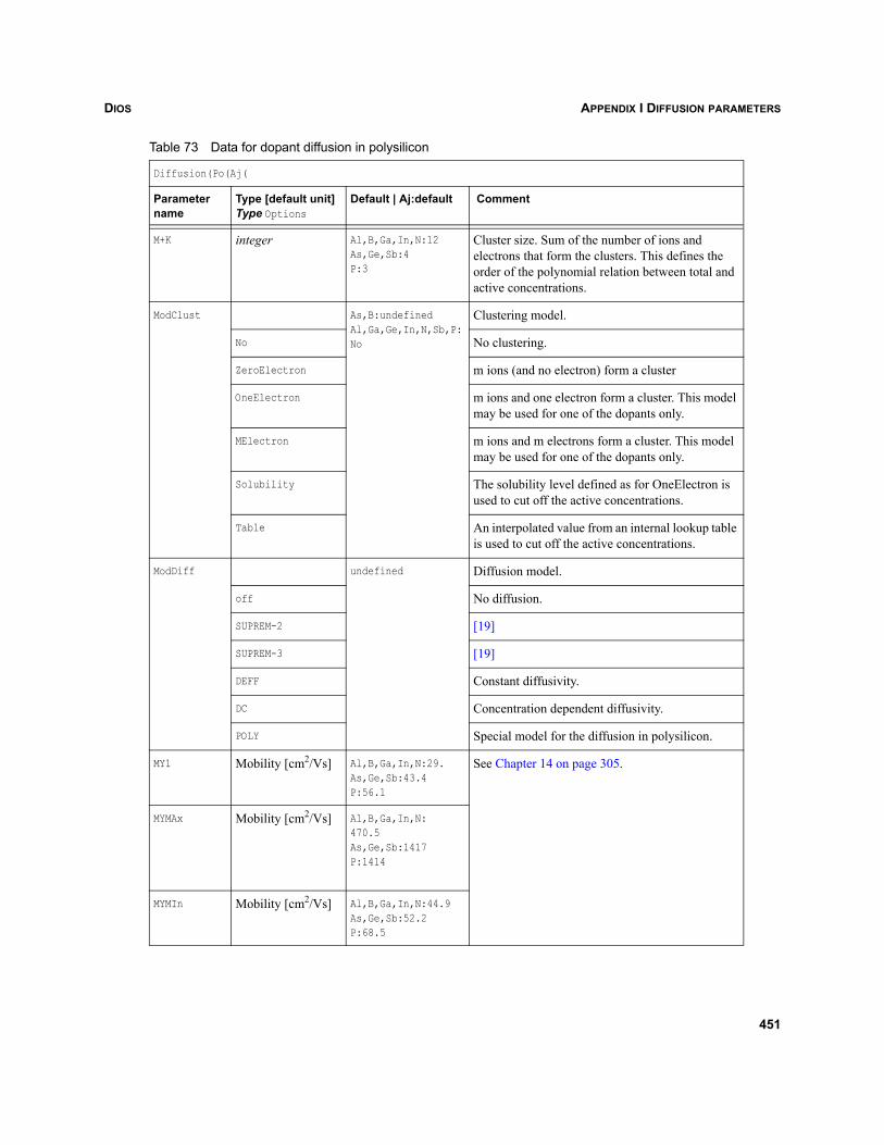
DIOS APPENDIX I DIFFUSION PARAMETERS
M+K integer Al,B,Ga,In,N:12As,Ge,Sb:4P:3
Cluster size. Sum of the number of ions and electrons that form the clusters. This defines the order of the polynomial relation between total and active concentrations.
ModClust As,B:undefinedAl,Ga,Ge,In,N,Sb,P: No
Clustering model.
No No clustering.
ZeroElectron m ions (and no electron) form a cluster
OneElectron m ions and one electron form a cluster. This model may be used for one of the dopants only.
MElectron m ions and m electrons form a cluster. This model may be used for one of the dopants only.
Solubility The solubility level defined as for OneElectron is used to cut off the active concentrations.
Table An interpolated value from an internal lookup table is used to cut off the active concentrations.
ModDiff undefined Diffusion model.
off No diffusion.
SUPREM-2 [19]
SUPREM-3 [19]
DEFF Constant diffusivity.
DC Concentration dependent diffusivity.
POLY Special model for the diffusion in polysilicon.
MY1 Mobility [cm2/Vs] Al,B,Ga,In,N:29.As,Ge,Sb:43.4P:56.1
See Chapter 14 on page 305.
MYMAx Mobility [cm2/Vs] Al,B,Ga,In,N:470.5As,Ge,Sb:1417P:1414
MYMIn Mobility [cm2/Vs] Al,B,Ga,In,N:44.9As,Ge,Sb:52.2P:68.5
Table 73 Data for dopant diffusion in polysilicon
Diffusion(Po(Aj(
Parameter name
Type [default unit]Type Options
Default | Aj:default Comment
451
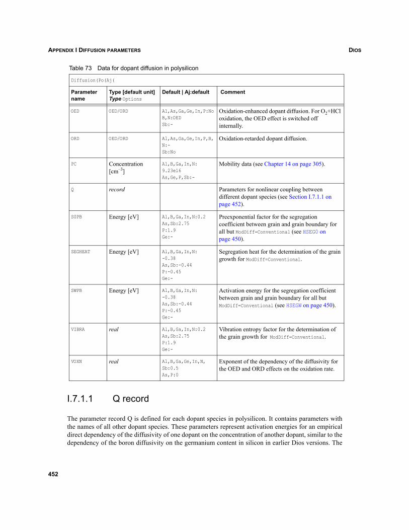
DIOSAPPENDIX I DIFFUSION PARAMETERS
I.7.1.1 Q record
The parameter record Q is defined for each dopant species in polysilicon. It contains parameters withthe names of all other dopant species. These parameters represent activation energies for an empiricaldirect dependency of the diffusivity of one dopant on the concentration of another dopant, similar to thedependency of the boron diffusivity on the germanium content in silicon in earlier Dios versions. The
OED OED/ORD Al,As,Ga,Ge,In,P:NoB,N:OEDSb:-
Oxidation-enhanced dopant diffusion. For O2+HCl oxidation, the OED effect is switched off internally.
ORD OED/ORD Al,As,Ga,Ge,In,P,B,N:-Sb:No
Oxidation-retarded dopant diffusion.
PC Concentration [cm–3]
Al,B,Ga,In,N:9.23e16As,Ge,P,Sb:-
Mobility data (see Chapter 14 on page 305).
Q record Parameters for nonlinear coupling between different dopant species (see Section I.7.1.1 on page 452).
S0PB Energy [eV] Al,B,Ga,In,N:0.2As,Sb:2.75P:1.9Ge:-
Preexponential factor for the segregation coefficient between grain and grain boundary for all but ModDiff=Conventional (see HSEG0 on page 450).
SEGHEAT Energy [eV] Al,B,Ga,In,N:-0.38As,Sb:-0.44P:-0.45Ge:-
Segregation heat for the determination of the grain growth for ModDiff=Conventional.
SWPB Energy [eV] Al,B,Ga,In,N:-0.38As,Sb:-0.44P:-0.45Ge:-
Activation energy for the segregation coefficient between grain and grain boundary for all but ModDiff=Conventional (see HSEGW on page 450).
VIBRA real Al,B,Ga,In,N:0.2As,Sb:2.75P:1.9Ge:-
Vibration entropy factor for the determination of the grain growth for ModDiff=Conventional.
VOXN real Al,B,Ga,Ge,In,N,Sb:0.5As,P:0
Exponent of the dependency of the diffusivity for the OED and ORD effects on the oxidation rate.
Table 73 Data for dopant diffusion in polysilicon
Diffusion(Po(Aj(
Parameter name
Type [default unit]Type Options
Default | Aj:default Comment
452
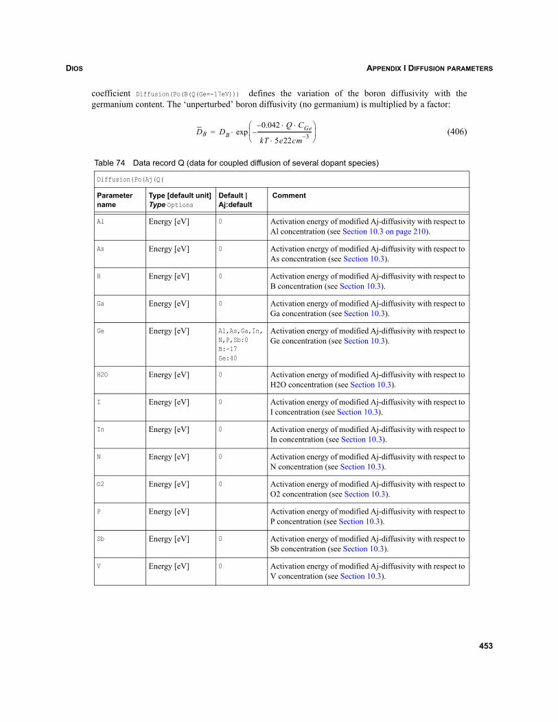
DIOS APPENDIX I DIFFUSION PARAMETERS
coefficient Diffusion(Po(B(Q(Ge=-17eV))) defines the variation of the boron diffusivity with thegermanium content. The ‘unperturbed’ boron diffusivity (no germanium) is multiplied by a factor:
(406)
Table 74 Data record Q (data for coupled diffusion of several dopant species)
Diffusion(Po(Aj(Q(
Parameter name
Type [default unit]Type Options
Default | Aj:default
Comment
Al Energy [eV] 0 Activation energy of modified Aj-diffusivity with respect to Al concentration (see Section 10.3 on page 210).
As Energy [eV] 0 Activation energy of modified Aj-diffusivity with respect to As concentration (see Section 10.3).
B Energy [eV] 0 Activation energy of modified Aj-diffusivity with respect to B concentration (see Section 10.3).
Ga Energy [eV] 0 Activation energy of modified Aj-diffusivity with respect to Ga concentration (see Section 10.3).
Ge Energy [eV] Al,As,Ga,In,N,P,Sb:0B:-17Ge:40
Activation energy of modified Aj-diffusivity with respect to Ge concentration (see Section 10.3).
H2O Energy [eV] 0 Activation energy of modified Aj-diffusivity with respect to H2O concentration (see Section 10.3).
I Energy [eV] 0 Activation energy of modified Aj-diffusivity with respect to I concentration (see Section 10.3).
In Energy [eV] 0 Activation energy of modified Aj-diffusivity with respect to In concentration (see Section 10.3).
N Energy [eV] 0 Activation energy of modified Aj-diffusivity with respect to N concentration (see Section 10.3).
O2 Energy [eV] 0 Activation energy of modified Aj-diffusivity with respect to O2 concentration (see Section 10.3).
P Energy [eV] Activation energy of modified Aj-diffusivity with respect to P concentration (see Section 10.3).
Sb Energy [eV] 0 Activation energy of modified Aj-diffusivity with respect to Sb concentration (see Section 10.3).
V Energy [eV] 0 Activation energy of modified Aj-diffusivity with respect to V concentration (see Section 10.3).
DB DB0.042 Q C⋅ ⋅– Ge
kT 5e22cm 3–⋅----------------------------------------–
⎝ ⎠⎜ ⎟⎛ ⎞
exp⋅=
453
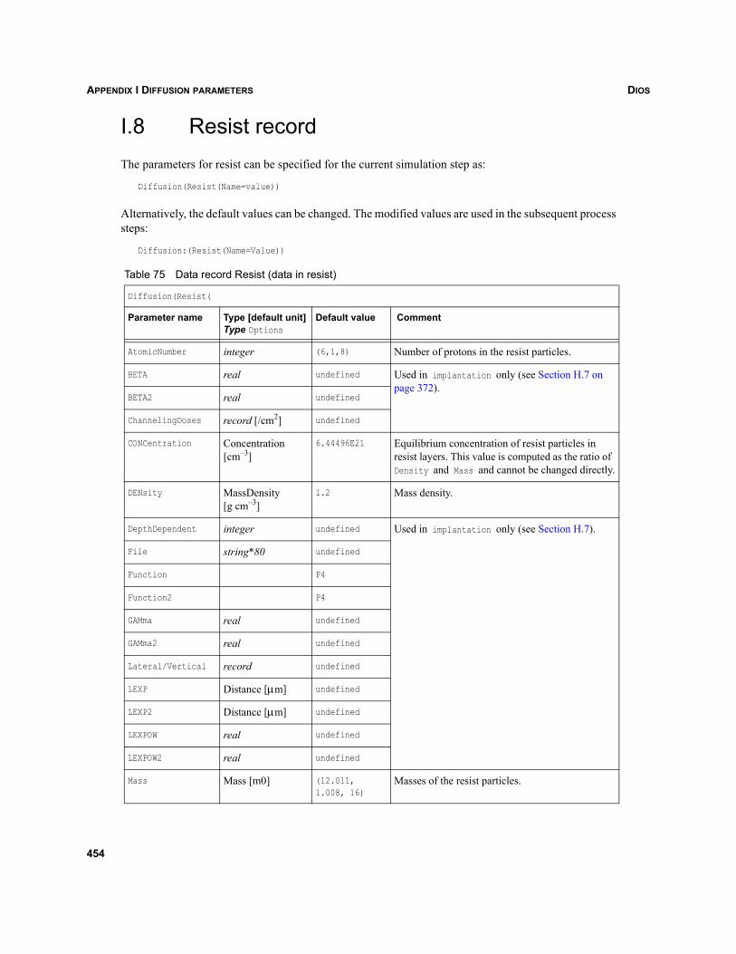
DIOSAPPENDIX I DIFFUSION PARAMETERS
I.8 Resist recordThe parameters for resist can be specified for the current simulation step as:
Diffusion(Resist(Name=value))
Alternatively, the default values can be changed. The modified values are used in the subsequent processsteps:
Diffusion:(Resist(Name=Value))
Table 75 Data record Resist (data in resist)
Diffusion(Resist(
Parameter name Type [default unit]Type Options
Default value Comment
AtomicNumber integer (6,1,8) Number of protons in the resist particles.
BETA real undefined Used in implantation only (see Section H.7 on page 372).
BETA2 real undefined
ChannelingDoses record [/cm2] undefined
CONCentration Concentration [cm–3]
6.44496E21 Equilibrium concentration of resist particles in resist layers. This value is computed as the ratio of Density and Mass and cannot be changed directly.
DENsity MassDensity [g cm–3]
1.2 Mass density.
DepthDependent integer undefined Used in implantation only (see Section H.7).
File string*80 undefined
Function P4
Function2 P4
GAMma real undefined
GAMma2 real undefined
Lateral/Vertical record undefined
LEXP Distance [μm] undefined
LEXP2 Distance [μm] undefined
LEXPOW real undefined
LEXPOW2 real undefined
Mass Mass [m0] (12.011, 1.008, 16)
Masses of the resist particles.
454
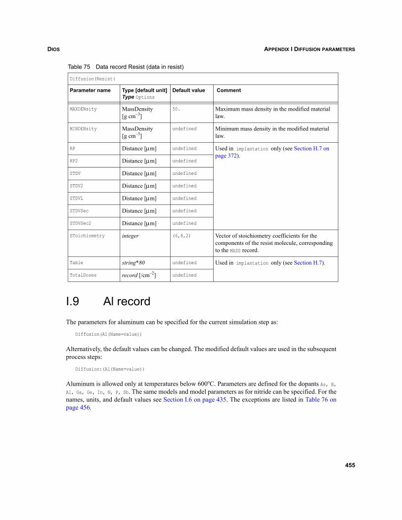
DIOS APPENDIX I DIFFUSION PARAMETERS
I.9 Al recordThe parameters for aluminum can be specified for the current simulation step as:
Diffusion(Al(Name=value))
Alternatively, the default values can be changed. The modified default values are used in the subsequentprocess steps:
Diffusion:(Al(Name=value))
Aluminum is allowed only at temperatures below 600oC. Parameters are defined for the dopants As, B,Al, Ga, Ge, In, N, P, Sb. The same models and model parameters as for nitride can be specified. For thenames, units, and default values see Section I.6 on page 435. The exceptions are listed in Table 76 onpage 456.
MAXDENsity MassDensity [g cm–3]
50. Maximum mass density in the modified material law.
MINDENsity MassDensity[g cm–3]
undefined Minimum mass density in the modified material law.
RP Distance [μm] undefined Used in implantation only (see Section H.7 on page 372).
RP2 Distance [μm] undefined
STDV Distance [μm] undefined
STDV2 Distance [μm] undefined
STDVL Distance [μm] undefined
STDVSec Distance [μm] undefined
STDVSec2 Distance [μm] undefined
SToichiometry integer (6,8,2) Vector of stoichiometry coefficients for the components of the resist molecule, corresponding to the MASS record.
Table string*80 undefined Used in implantation only (see Section H.7).
TotalDoses record [/cm–2] undefined
Table 75 Data record Resist (data in resist)
Diffusion(Resist(
Parameter name Type [default unit]Type Options
Default value Comment
455
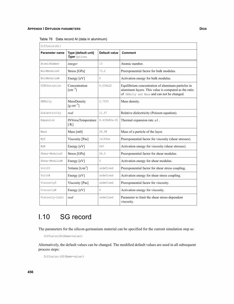
DIOSAPPENDIX I DIFFUSION PARAMETERS
I.10 SG recordThe parameters for the silicon-germanium material can be specified for the current simulation step as:
Diffusion(SG(Name=value))
Alternatively, the default values can be changed. The modified default values are used in all subsequentprocess steps:
Diffusion:(SG(Name=value))
Table 76 Data record Al (data in aluminum)
Diffusion(Al(
Parameter name Type [default unit]Type Options
Default value Comment
AtomicNumber integer 13 Atomic number.
BulkModulus0 Stress [GPa] 73.2 Preexponential factor for bulk modulus.
BulkModulusW Energy [eV] 0 Activation energy for bulk modulus.
CONCentration Concentration [cm–3]
6.034e22 Equilibrium concentration of aluminum particles in aluminum layers. This value is computed as the ratio of DENsity and Mass and can not be changed.
DENsity MassDensity [g cm–3]
2.7033 Mass density.
Dielectricity real 11.67 Relative dielectricity (Poisson equation).
Expansion INVerseTemperature [/K]
8.439685e-05 Thermal expansion rate .
Mass Mass [m0] 26.98 Mass of a particle of the layer.
My0 Viscosity [Pas] 1e14Pas Preexponential factor for viscosity (shear stresses).
MyW Energy [eV] 0eV Activation energy for viscosity (shear stresses).
Shear-Modulus0 Stress [GPa] 26.0 Preexponential factor for shear modulus.
Shear-ModulusW Energy [eV] 0 Activation energy for shear modulus.
vcrit0 Volume [υm3] undefined Preexponential factor for shear stress coupling.
VcritW Energy [eV] undefined Activation energy for shear stress coupling.
Viscosity0 Viscosity [Pas] undefined Preexponential factor for viscosity.
ViscosityW Energy [eV] 0 Activation energy for viscosity.
Viscosity-Limit real undefined Parameter to limit the shear stress-dependent viscosity.
a1
456
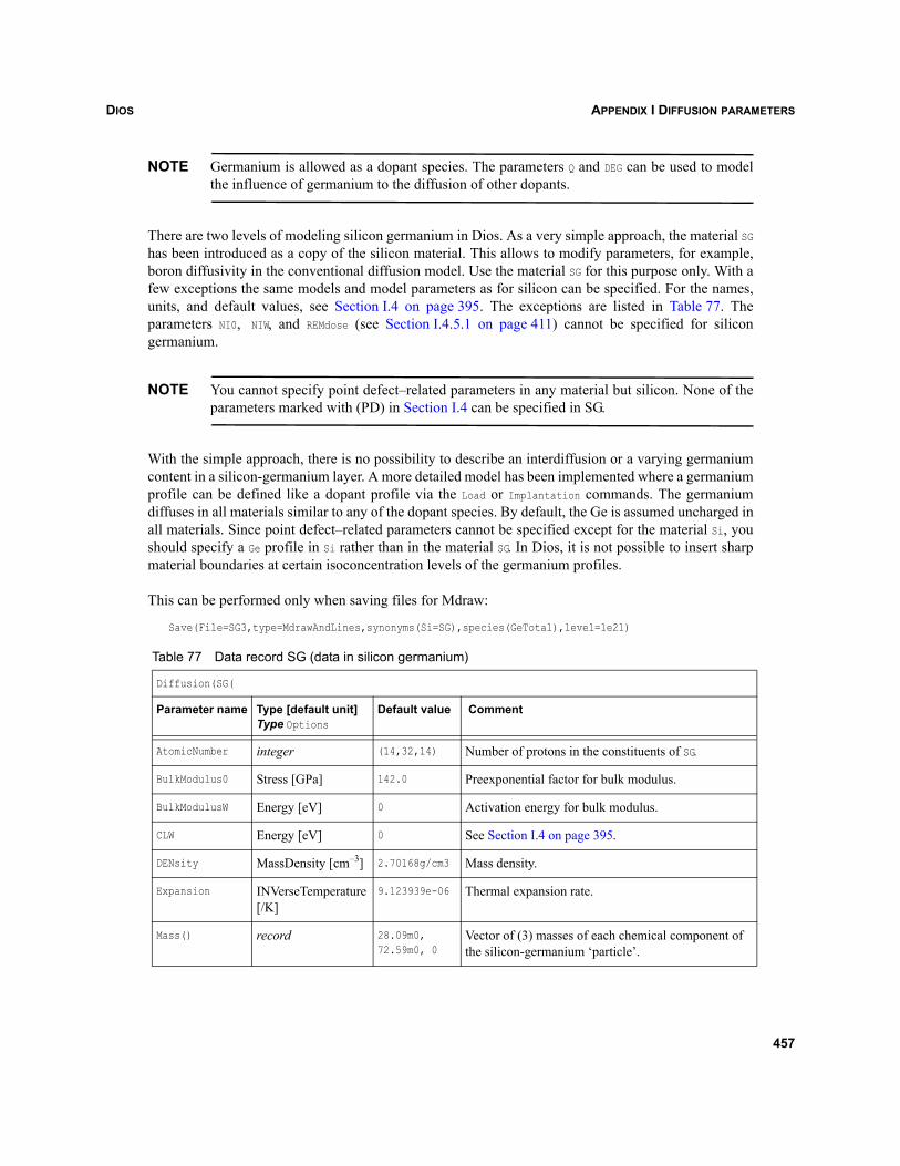
DIOS APPENDIX I DIFFUSION PARAMETERS
NOTE Germanium is allowed as a dopant species. The parameters Q and DEG can be used to modelthe influence of germanium to the diffusion of other dopants.
There are two levels of modeling silicon germanium in Dios. As a very simple approach, the material SGhas been introduced as a copy of the silicon material. This allows to modify parameters, for example,boron diffusivity in the conventional diffusion model. Use the material SG for this purpose only. With afew exceptions the same models and model parameters as for silicon can be specified. For the names,units, and default values, see Section I.4 on page 395. The exceptions are listed in Table 77. Theparameters NI0, NIW, and REMdose (see Section I.4.5.1 on page 411) cannot be specified for silicongermanium.
NOTE You cannot specify point defect–related parameters in any material but silicon. None of theparameters marked with (PD) in Section I.4 can be specified in SG.
With the simple approach, there is no possibility to describe an interdiffusion or a varying germaniumcontent in a silicon-germanium layer. A more detailed model has been implemented where a germaniumprofile can be defined like a dopant profile via the Load or Implantation commands. The germaniumdiffuses in all materials similar to any of the dopant species. By default, the Ge is assumed uncharged inall materials. Since point defect–related parameters cannot be specified except for the material Si, youshould specify a Ge profile in Si rather than in the material SG. In Dios, it is not possible to insert sharpmaterial boundaries at certain isoconcentration levels of the germanium profiles.
This can be performed only when saving files for Mdraw:
Save(File=SG3,type=MdrawAndLines,synonyms(Si=SG),species(GeTotal),level=1e21)
Table 77 Data record SG (data in silicon germanium)
Diffusion(SG(
Parameter name Type [default unit]Type Options
Default value Comment
AtomicNumber integer (14,32,14) Number of protons in the constituents of SG.
BulkModulus0 Stress [GPa] 142.0 Preexponential factor for bulk modulus.
BulkModulusW Energy [eV] 0 Activation energy for bulk modulus.
CLW Energy [eV] 0 See Section I.4 on page 395.
DENsity MassDensity [cm–3] 2.70168g/cm3 Mass density.
Expansion INVerseTemperature [/K]
9.123939e-06 Thermal expansion rate.
Mass() record 28.09m0,72.59m0, 0
Vector of (3) masses of each chemical component of the silicon-germanium ‘particle’.
457
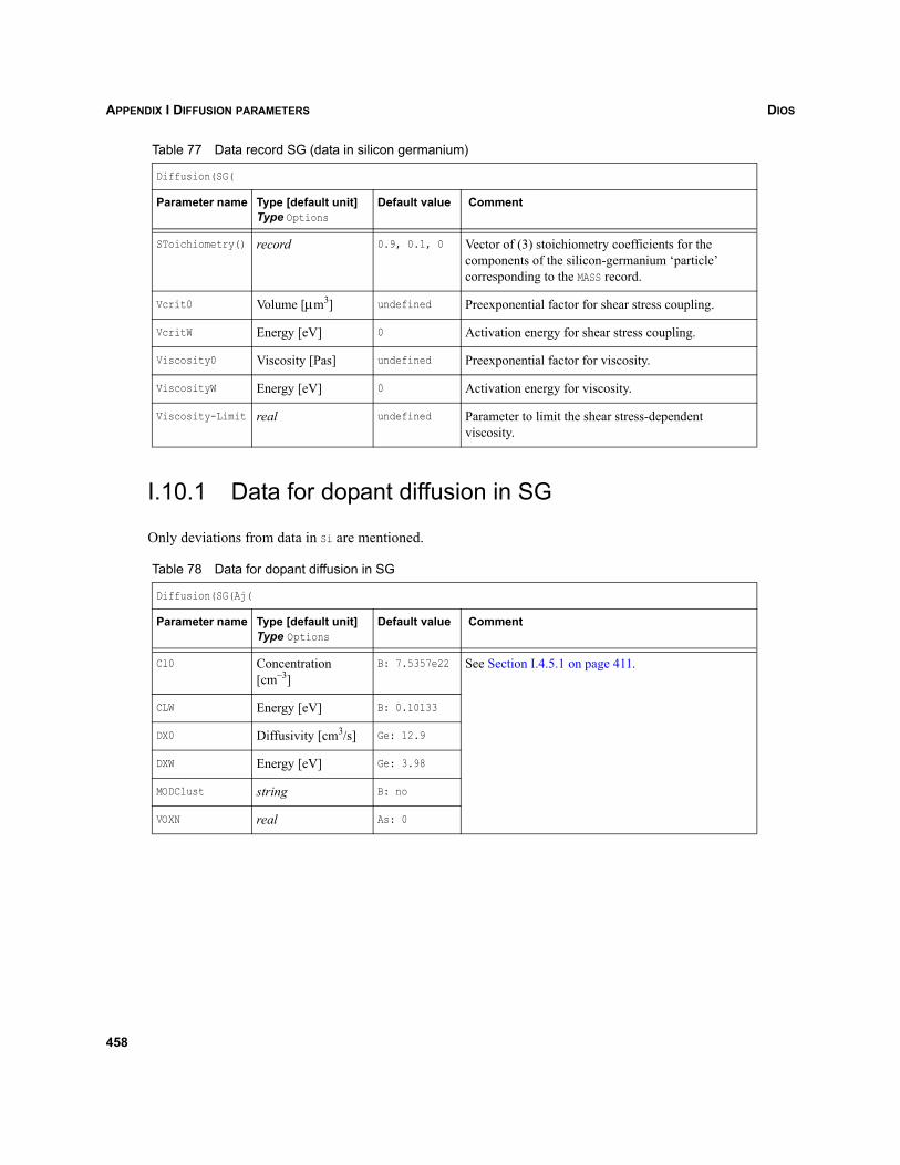
DIOSAPPENDIX I DIFFUSION PARAMETERS
I.10.1 Data for dopant diffusion in SG
Only deviations from data in Si are mentioned.
SToichiometry() record 0.9, 0.1, 0 Vector of (3) stoichiometry coefficients for the components of the silicon-germanium ‘particle’ corresponding to the MASS record.
Vcrit0 Volume [μm3] undefined Preexponential factor for shear stress coupling.
VcritW Energy [eV] 0 Activation energy for shear stress coupling.
Viscosity0 Viscosity [Pas] undefined Preexponential factor for viscosity.
ViscosityW Energy [eV] 0 Activation energy for viscosity.
Viscosity-Limit real undefined Parameter to limit the shear stress-dependent viscosity.
Table 78 Data for dopant diffusion in SG
Diffusion(SG(Aj(
Parameter name Type [default unit]Type Options
Default value Comment
Cl0 Concentration [cm–3]
B: 7.5357e22 See Section I.4.5.1 on page 411.
CLW Energy [eV] B: 0.10133
DX0 Diffusivity [cm3/s] Ge: 12.9
DXW Energy [eV] Ge: 3.98
MODClust string B: no
VOXN real As: 0
Table 77 Data record SG (data in silicon germanium)
Diffusion(SG(
Parameter name Type [default unit]Type Options
Default value Comment
458
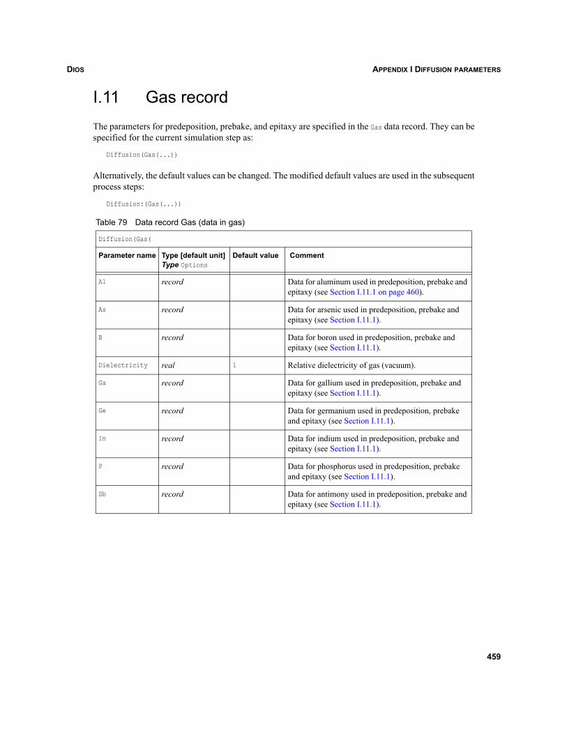
DIOS APPENDIX I DIFFUSION PARAMETERS
I.11 Gas recordThe parameters for predeposition, prebake, and epitaxy are specified in the Gas data record. They can bespecified for the current simulation step as:
Diffusion(Gas(...))
Alternatively, the default values can be changed. The modified default values are used in the subsequentprocess steps:
Diffusion:(Gas(...))
Table 79 Data record Gas (data in gas)
Diffusion(Gas(
Parameter name Type [default unit]Type Options
Default value Comment
Al record Data for aluminum used in predeposition, prebake and epitaxy (see Section I.11.1 on page 460).
As record Data for arsenic used in predeposition, prebake and epitaxy (see Section I.11.1).
B record Data for boron used in predeposition, prebake and epitaxy (see Section I.11.1).
Dielectricity real 1 Relative dielectricity of gas (vacuum).
Ga record Data for gallium used in predeposition, prebake and epitaxy (see Section I.11.1).
Ge record Data for germanium used in predeposition, prebake and epitaxy (see Section I.11.1).
In record Data for indium used in predeposition, prebake and epitaxy (see Section I.11.1).
P record Data for phosphorus used in predeposition, prebake and epitaxy (see Section I.11.1).
Sb record Data for antimony used in predeposition, prebake and epitaxy (see Section I.11.1).
459
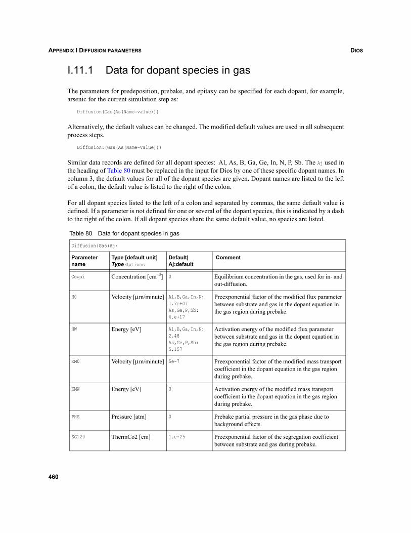
DIOSAPPENDIX I DIFFUSION PARAMETERS
I.11.1 Data for dopant species in gas
The parameters for predeposition, prebake, and epitaxy can be specified for each dopant, for example,arsenic for the current simulation step as:
Diffusion(Gas(As(Name=value)))
Alternatively, the default values can be changed. The modified default values are used in all subsequentprocess steps.
Diffusion:(Gas(As(Name=value)))
Similar data records are defined for all dopant species: Al, As, B, Ga, Ge, In, N, P, Sb. The Aj used inthe heading of Table 80 must be replaced in the input for Dios by one of these specific dopant names. Incolumn 3, the default values for all of the dopant species are given. Dopant names are listed to the leftof a colon, the default value is listed to the right of the colon.
For all dopant species listed to the left of a colon and separated by commas, the same default value isdefined. If a parameter is not defined for one or several of the dopant species, this is indicated by a dashto the right of the colon. If all dopant species share the same default value, no species are listed.
Table 80 Data for dopant species in gas
Diffusion(Gas(Aj(
Parameter name
Type [default unit]Type Options
Default|Aj:default
Comment
Cequi Concentration [cm–3] 0 Equilibrium concentration in the gas, used for in- and out-diffusion.
H0 Velocity [μm/minute] Al,B,Ga,In,N:1.7e+07As,Ge,P,Sb:6.e+17
Preexponential factor of the modified flux parameter between substrate and gas in the dopant equation in the gas region during prebake.
HW Energy [eV] Al,B,Ga,In,N:2.48As,Ge,P,Sb:5.157
Activation energy of the modified flux parameter between substrate and gas in the dopant equation in the gas region during prebake.
KM0 Velocity [μm/minute] 5e-7 Preexponential factor of the modified mass transport coefficient in the dopant equation in the gas region during prebake.
KMW Energy [eV] 0 Activation energy of the modified mass transport coefficient in the dopant equation in the gas region during prebake.
PHS Pressure [atm] 0 Prebake partial pressure in the gas phase due to background effects.
SG120 ThermCo2 [cm] 1.e-25 Preexponential factor of the segregation coefficient between substrate and gas during prebake.
460
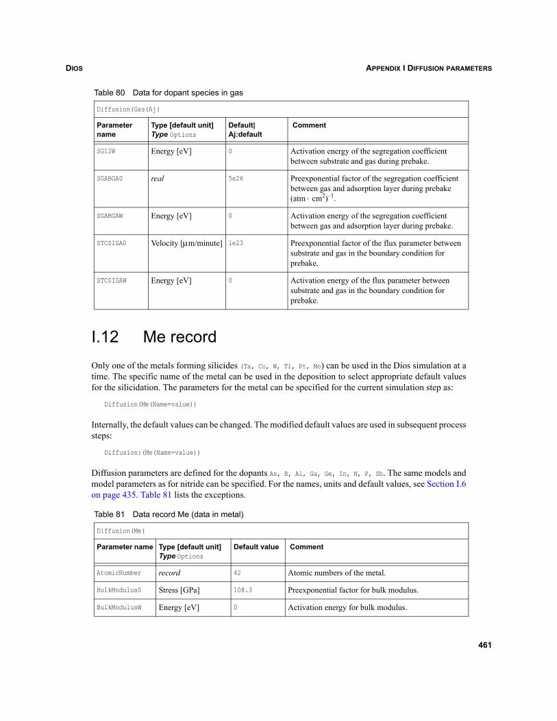
DIOS APPENDIX I DIFFUSION PARAMETERS
I.12 Me recordOnly one of the metals forming silicides (Ta, Co, W, Ti, Pt, Mo) can be used in the Dios simulation at atime. The specific name of the metal can be used in the deposition to select appropriate default valuesfor the silicidation. The parameters for the metal can be specified for the current simulation step as:
Diffusion(Me(Name=value))
Internally, the default values can be changed. The modified default values are used in subsequent processsteps:
Diffusion:(Me(Name=value))
Diffusion parameters are defined for the dopants As, B, Al, Ga, Ge, In, N, P, Sb. The same models andmodel parameters as for nitride can be specified. For the names, units and default values, see Section I.6on page 435. Table 81 lists the exceptions.
SG12W Energy [eV] 0 Activation energy of the segregation coefficient between substrate and gas during prebake.
SGABGA0 real 5e26 Preexponential factor of the segregation coefficient between gas and adsorption layer during prebake (atm ⋅ cm2)–1.
SGABGAW Energy [eV] 0 Activation energy of the segregation coefficient between gas and adsorption layer during prebake.
STCSIGA0 Velocity [μm/minute] 1e23 Preexponential factor of the flux parameter between substrate and gas in the boundary condition for prebake.
STCSIGAW Energy [eV] 0 Activation energy of the flux parameter between substrate and gas in the boundary condition for prebake.
Table 81 Data record Me (data in metal)
Diffusion(Me(
Parameter name Type [default unit]Type Options
Default value Comment
AtomicNumber record 42 Atomic numbers of the metal.
BulkModulus0 Stress [GPa] 108.3 Preexponential factor for bulk modulus.
BulkModulusW Energy [eV] 0 Activation energy for bulk modulus.
Table 80 Data for dopant species in gas
Diffusion(Gas(Aj(
Parameter name
Type [default unit]Type Options
Default|Aj:default
Comment
461
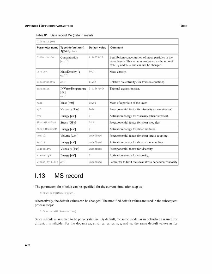
DIOSAPPENDIX I DIFFUSION PARAMETERS
I.13 MS recordThe parameters for silicide can be specified for the current simulation step as:
Diffusion(MS(Name=value))
Alternatively, the default values can be changed. The modified default values are used in the subsequentprocess steps:
Diffusion:(MS(Name=value))
Since silicide is assumed to be polycrystalline. By default, the same model as in polysilicon is used fordiffusion in silicide. For the dopants As, B, Al, Ga, Ge, In, N, P, and Sb, the same default values as for
CONCentration Concentration [cm–3]
6.40255e22 Equilibrium concentration of metal particles in the metal layers. This value is computed as the ratio of DENsity and Mass and can not be changed.
DENsity MassDensity [g cm–3]
10.2 Mass density.
Dielectricity real 11.67 Relative dielectricity (for Poisson equation).
Expansion INVerseTemperature [/K]real
2.41667e-06 Thermal expansion rate.
Mass Mass [m0] 95.94 Mass of a particle of the layer.
My0 Viscosity [Pas] 1e14 Preexponential factor for viscosity (shear stresses).
MyW Energy [eV] 0 Activation energy for viscosity (shear stresses).
Shear-Modulus0 Stress [GPa] 38.8 Preexponential factor for shear modulus.
Shear-ModulusW Energy [eV] 0 Activation energy for shear modulus.
Vcrit0 Volume [μm3] undefined Preexponential factor for shear stress coupling.
VcritW Energy [eV] undefined Activation energy for shear stress coupling.
Viscosity0 Viscosity [Pas] undefined Preexponential factor for viscosity.
ViscosityW Energy [eV] 0 Activation energy for viscosity.
Viscosity-Limit real undefined Parameter to limit the shear stress-dependent viscosity
Table 81 Data record Me (data in metal)
Diffusion(Me(
Parameter name Type [default unit]Type Options
Default value Comment
462
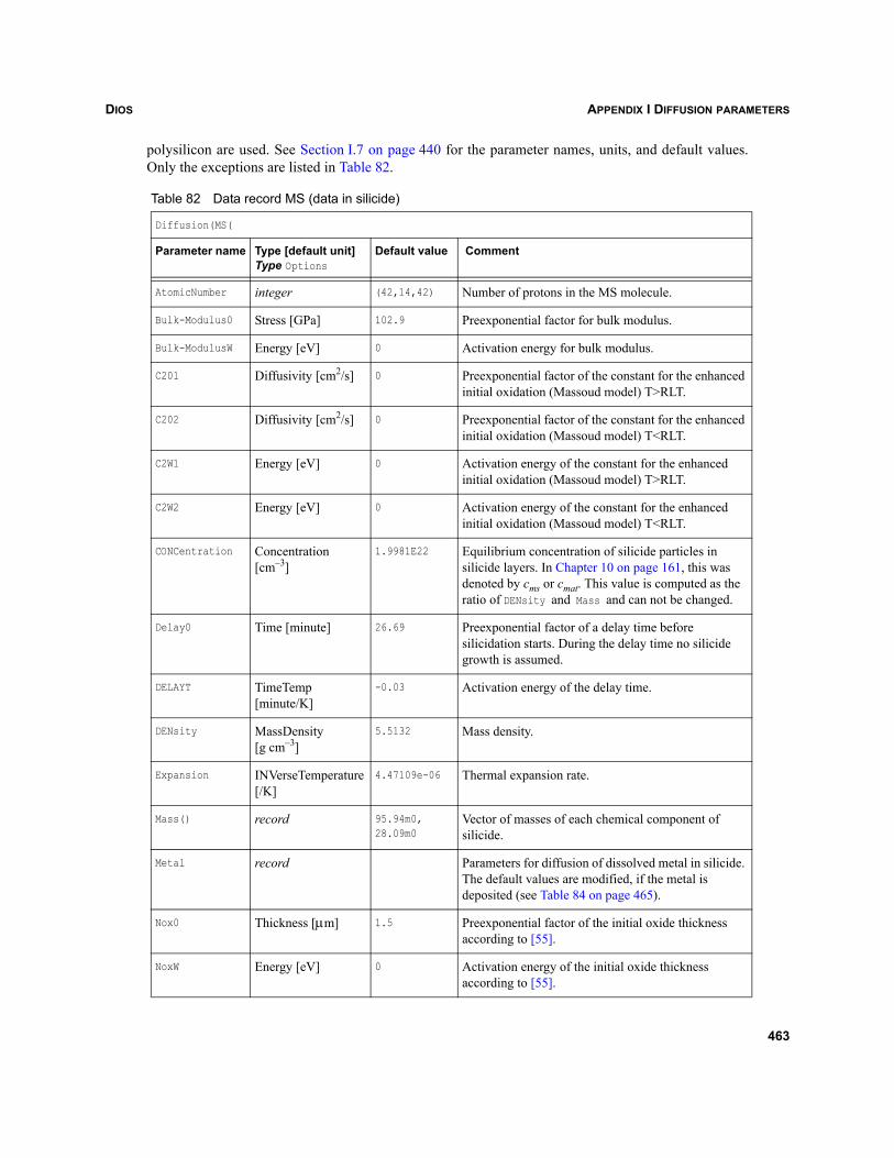
DIOS APPENDIX I DIFFUSION PARAMETERS
polysilicon are used. See Section I.7 on page 440 for the parameter names, units, and default values.Only the exceptions are listed in Table 82.
Table 82 Data record MS (data in silicide)
Diffusion(MS(
Parameter name Type [default unit]Type Options
Default value Comment
AtomicNumber integer (42,14,42) Number of protons in the MS molecule.
Bulk-Modulus0 Stress [GPa] 102.9 Preexponential factor for bulk modulus.
Bulk-ModulusW Energy [eV] 0 Activation energy for bulk modulus.
C201 Diffusivity [cm2/s] 0 Preexponential factor of the constant for the enhanced initial oxidation (Massoud model) T>RLT.
C202 Diffusivity [cm2/s] 0 Preexponential factor of the constant for the enhanced initial oxidation (Massoud model) T<RLT.
C2W1 Energy [eV] 0 Activation energy of the constant for the enhanced initial oxidation (Massoud model) T>RLT.
C2W2 Energy [eV] 0 Activation energy of the constant for the enhanced initial oxidation (Massoud model) T<RLT.
CONCentration Concentration [cm–3]
1.9981E22 Equilibrium concentration of silicide particles in silicide layers. In Chapter 10 on page 161, this was denoted by cms or cmat. This value is computed as the ratio of DENsity and Mass and can not be changed.
Delay0 Time [minute] 26.69 Preexponential factor of a delay time before silicidation starts. During the delay time no silicide growth is assumed.
DELAYT TimeTemp[minute/K]
-0.03 Activation energy of the delay time.
DENsity MassDensity [g cm–3]
5.5132 Mass density.
Expansion INVerseTemperature [/K]
4.47109e-06 Thermal expansion rate.
Mass() record 95.94m0, 28.09m0
Vector of masses of each chemical component of silicide.
Metal record Parameters for diffusion of dissolved metal in silicide. The default values are modified, if the metal is deposited (see Table 84 on page 465).
Nox0 Thickness [μm] 1.5 Preexponential factor of the initial oxide thickness according to [55].
NoxW Energy [eV] 0 Activation energy of the initial oxide thickness according to [55].
463
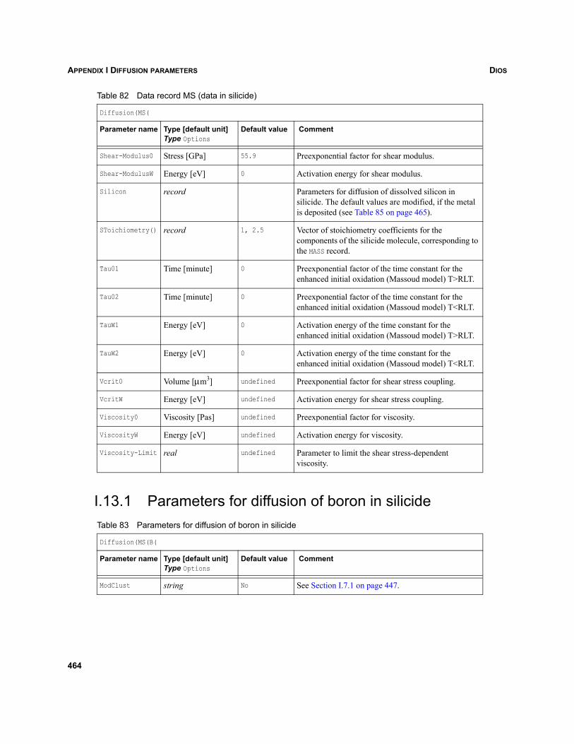
DIOSAPPENDIX I DIFFUSION PARAMETERS
I.13.1 Parameters for diffusion of boron in silicide
Shear-Modulus0 Stress [GPa] 55.9 Preexponential factor for shear modulus.
Shear-ModulusW Energy [eV] 0 Activation energy for shear modulus.
Silicon record Parameters for diffusion of dissolved silicon in silicide. The default values are modified, if the metal is deposited (see Table 85 on page 465).
SToichiometry() record 1, 2.5 Vector of stoichiometry coefficients for the components of the silicide molecule, corresponding to the MASS record.
Tau01 Time [minute] 0 Preexponential factor of the time constant for the enhanced initial oxidation (Massoud model) T>RLT.
Tau02 Time [minute] 0 Preexponential factor of the time constant for the enhanced initial oxidation (Massoud model) T<RLT.
TauW1 Energy [eV] 0 Activation energy of the time constant for the enhanced initial oxidation (Massoud model) T>RLT.
TauW2 Energy [eV] 0 Activation energy of the time constant for the enhanced initial oxidation (Massoud model) T<RLT.
Vcrit0 Volume [μm3] undefined Preexponential factor for shear stress coupling.
VcritW Energy [eV] undefined Activation energy for shear stress coupling.
Viscosity0 Viscosity [Pas] undefined Preexponential factor for viscosity.
ViscosityW Energy [eV] undefined Activation energy for viscosity.
Viscosity-Limit real undefined Parameter to limit the shear stress-dependent viscosity.
Table 83 Parameters for diffusion of boron in silicide
Diffusion(MS(B(
Parameter name Type [default unit]Type Options
Default value Comment
ModClust string No See Section I.7.1 on page 447.
Table 82 Data record MS (data in silicide)
Diffusion(MS(
Parameter name Type [default unit]Type Options
Default value Comment
464
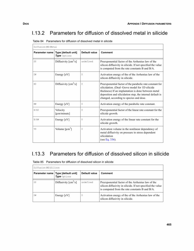
DIOS APPENDIX I DIFFUSION PARAMETERS
I.13.2 Parameters for diffusion of dissolved metal in silicide
I.13.3 Parameters for diffusion of dissolved silicon in silicide
Table 84 Parameters for diffusion of dissolved metal in silicide
Diffusion(MS(Metal
Parameter name Type [default unit]Type Options
Default value Comment
D0 Diffusivity [cm2/s] undefined Preexponential factor of the Arrhenius law of the silicon diffusivity in silicide. If not specified the value is computed from the rate constants B and B/A.
DW Energy [eV] 0 Activation energy of the of the Arrhenius law of the silicon diffusivity in silicide.
B0 Diffusivity [cm2/s] 0 Preexponential factor of the parabolic rate constant for silicidation. (Deal–Grove model for 1D silicide thickness) If an implantation is done between metal deposition and silicidation step, the internal default is changed, according to species and dose.
BW Energy [eV] 0 Activation energy of the parabolic rate constant.
B/A0 Velocity [μm/minute]
0 Preexponential factor of the linear rate constant for the silicide growth.
B/AW Energy [eV] 0 Activation energy of the linear rate constant for the silicide growth.
VD Volume [μm3] 0 Activation volume in the nonlinear dependency of metal diffusivity on pressure in stress dependent silicidation (see Eq. 336).
Table 85 Parameters for diffusion of dissolved silicon in silicide
Diffusion(MS(Silicon
Parameter name Type [default unit]Type Options
Default value Comment
D0 Diffusivity [cm2/s] undefined Preexponential factor of the Arrhenius law of the silicon diffusivity in silicide. If not specified the value is computed from the rate constants B and B/A.
DW Energy [eV] 0 Activation energy of the of the Arrhenius law of the silicon diffusivity in silicide.
465
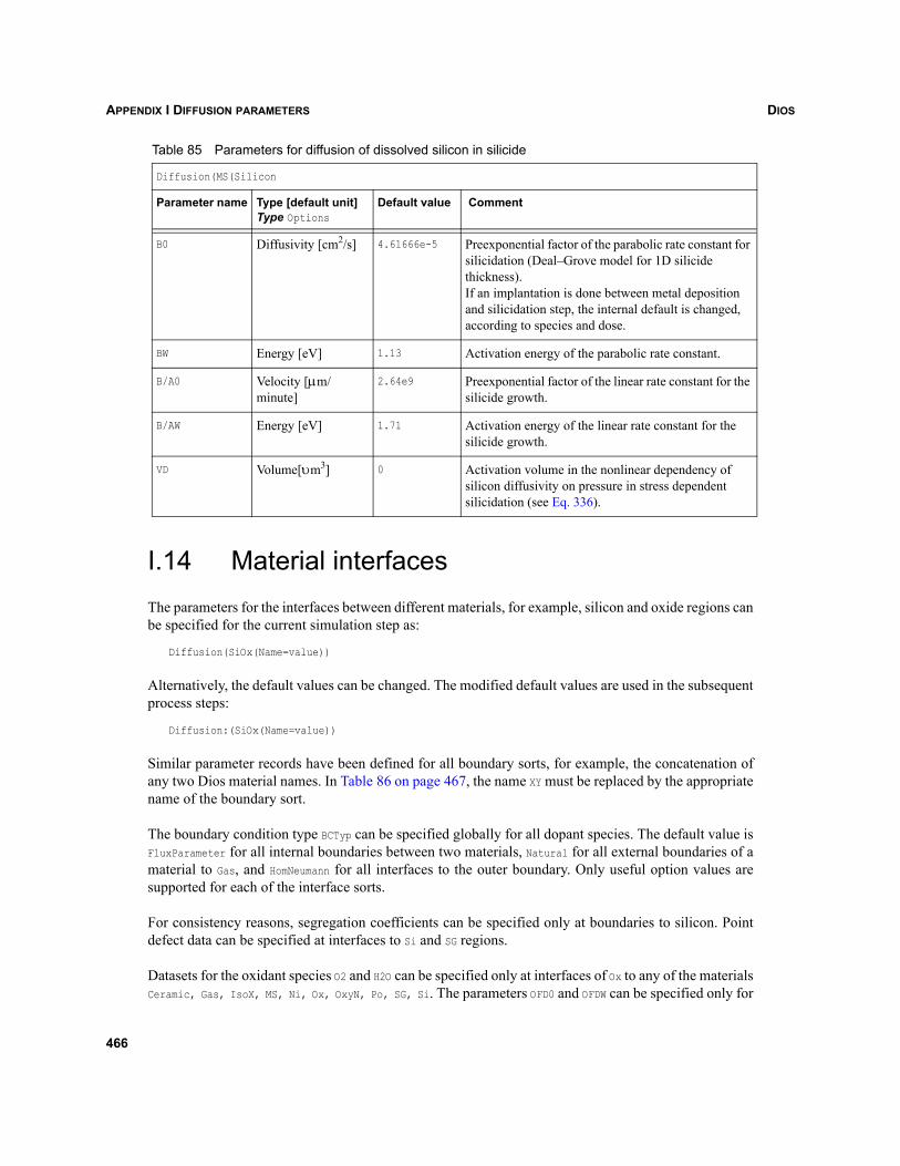
DIOSAPPENDIX I DIFFUSION PARAMETERS
I.14 Material interfacesThe parameters for the interfaces between different materials, for example, silicon and oxide regions canbe specified for the current simulation step as:
Diffusion(SiOx(Name=value))
Alternatively, the default values can be changed. The modified default values are used in the subsequentprocess steps:
Diffusion:(SiOx(Name=value))
Similar parameter records have been defined for all boundary sorts, for example, the concatenation ofany two Dios material names. In Table 86 on page 467, the name XY must be replaced by the appropriatename of the boundary sort.
The boundary condition type BCTyp can be specified globally for all dopant species. The default value isFluxParameter for all internal boundaries between two materials, Natural for all external boundaries of amaterial to Gas, and HomNeumann for all interfaces to the outer boundary. Only useful option values aresupported for each of the interface sorts.
For consistency reasons, segregation coefficients can be specified only at boundaries to silicon. Pointdefect data can be specified at interfaces to Si and SG regions.
Datasets for the oxidant species O2 and H2O can be specified only at interfaces of Ox to any of the materialsCeramic, Gas, IsoX, MS, Ni, Ox, OxyN, Po, SG, Si. The parameters OFD0 and OFDW can be specified only for
B0 Diffusivity [cm2/s] 4.61666e-5 Preexponential factor of the parabolic rate constant for silicidation (Deal–Grove model for 1D silicide thickness). If an implantation is done between metal deposition and silicidation step, the internal default is changed, according to species and dose.
BW Energy [eV] 1.13 Activation energy of the parabolic rate constant.
B/A0 Velocity [μm/minute]
2.64e9 Preexponential factor of the linear rate constant for the silicide growth.
B/AW Energy [eV] 1.71 Activation energy of the linear rate constant for the silicide growth.
VD Volume[υm3] 0 Activation volume in the nonlinear dependency of silicon diffusivity on pressure in stress dependent silicidation (see Eq. 336).
Table 85 Parameters for diffusion of dissolved silicon in silicide
Diffusion(MS(Silicon
Parameter name Type [default unit]Type Options
Default value Comment
466
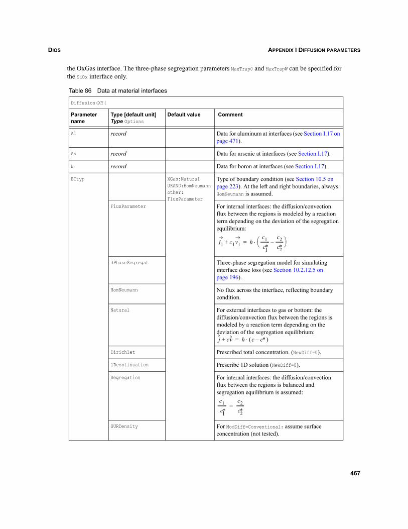
DIOS APPENDIX I DIFFUSION PARAMETERS
the OxGas interface. The three-phase segregation parameters MaxTrap0 and MaxTrapW can be specified forthe SiOx interface only.
Table 86 Data at material interfaces
Diffusion(XY(
Parameter name
Type [default unit]Type Options
Default value Comment
Al record Data for aluminum at interfaces (see Section I.17 on page 471).
As record Data for arsenic at interfaces (see Section I.17).
B record Data for boron at interfaces (see Section I.17).
BCtyp XGas:NaturalURAND:HomNeumannother:FluxParameter
Type of boundary condition (see Section 10.5 on page 223). At the left and right boundaries, always HomNeumann is assumed.
FluxParameter For internal interfaces: the diffusion/convection flux between the regions is modeled by a reaction term depending on the deviation of the segregation equilibrium:
3PhaseSegregat Three-phase segregation model for simulating interface dose loss (see Section 10.2.12.5 on page 196).
HomNeumann No flux across the interface, reflecting boundary condition.
Natural For external interfaces to gas or bottom: the diffusion/convection flux between the regions is modeled by a reaction term depending on the deviation of the segregation equilibrium:
Dirichlet Prescribed total concentration. (NewDiff=0).
1Dcontinuation Prescribe 1D solution (NewDiff=0).
Segregation For internal interfaces: the diffusion/convection flux between the regions is balanced and segregation equilibrium is assumed:
SURDensity For ModDiff=Conventional: assume surface concentration (not tested).
j1 c1v1+ hc1
c∗1---------
c2
c∗2
--------–⎝ ⎠⎛ ⎞⋅=
j cv+ h c c∗–( )⋅=
c1
c∗1---------
c2
c∗2
--------=
467
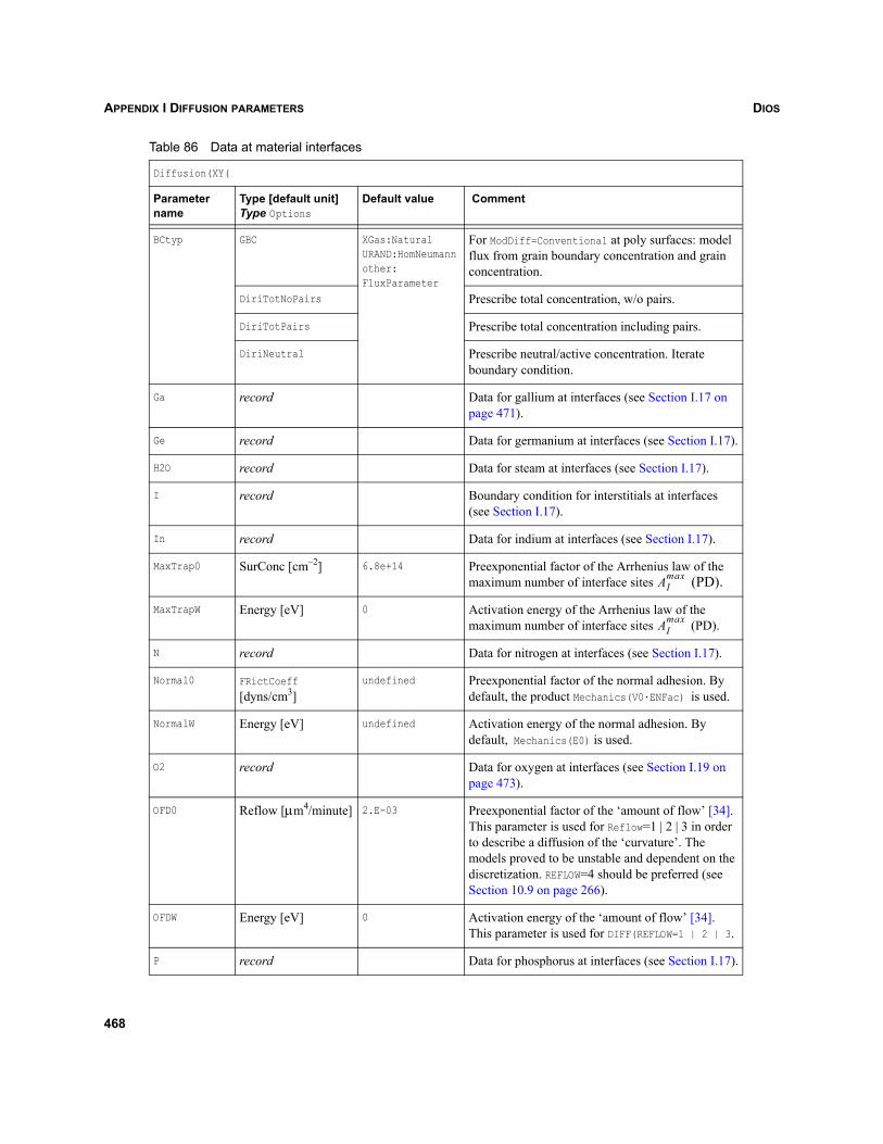
DIOSAPPENDIX I DIFFUSION PARAMETERS
BCtyp GBC XGas:NaturalURAND:HomNeumannother:FluxParameter
For ModDiff=Conventional at poly surfaces: model flux from grain boundary concentration and grain concentration.
DiriTotNoPairs Prescribe total concentration, w/o pairs.
DiriTotPairs Prescribe total concentration including pairs.
DiriNeutral Prescribe neutral/active concentration. Iterate boundary condition.
Ga record Data for gallium at interfaces (see Section I.17 on page 471).
Ge record Data for germanium at interfaces (see Section I.17).
H2O record Data for steam at interfaces (see Section I.17).
I record Boundary condition for interstitials at interfaces (see Section I.17).
In record Data for indium at interfaces (see Section I.17).
MaxTrap0 SurConc [cm–2] 6.8e+14 Preexponential factor of the Arrhenius law of the maximum number of interface sites (PD).
MaxTrapW Energy [eV] 0 Activation energy of the Arrhenius law of the maximum number of interface sites (PD).
N record Data for nitrogen at interfaces (see Section I.17).
Normal0 FRictCoeff [dyns/cm3]
undefined Preexponential factor of the normal adhesion. By default, the product Mechanics(V0·ENFac) is used.
NormalW Energy [eV] undefined Activation energy of the normal adhesion. By default, Mechanics(E0) is used.
O2 record Data for oxygen at interfaces (see Section I.19 on page 473).
OFD0 Reflow [μm4/minute] 2.E-03 Preexponential factor of the ‘amount of flow’ [34]. This parameter is used for Reflow=1 | 2 | 3 in order to describe a diffusion of the ‘curvature’. The models proved to be unstable and dependent on the discretization. REFLOW=4 should be preferred (see Section 10.9 on page 266).
OFDW Energy [eV] 0 Activation energy of the ‘amount of flow’ [34]. This parameter is used for DIFF(REFLOW=1 | 2 | 3.
P record Data for phosphorus at interfaces (see Section I.17).
Table 86 Data at material interfaces
Diffusion(XY(
Parameter name
Type [default unit]Type Options
Default value Comment
AImax
AImax
468
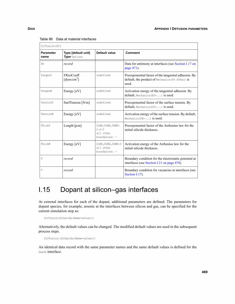
DIOS APPENDIX I DIFFUSION PARAMETERS
I.15 Dopant at silicon–gas interfacesAt external interfaces for each of the dopant, additional parameters are defined. The parameters fordopant species, for example, arsenic at the interfaces between silicon and gas, can be specified for thecurrent simulation step as:
Diffusion(SiGas(As(Name=value)))
Alternatively, the default values can be changed. The modified default values are used in the subsequentprocess steps.
Diffusion:(SiGas(As(Name=value)))
An identical data record with the same parameter names and the same default values is defined for theGasSG interface.
Sb record Data for antimony at interfaces (see Section I.17 on page 471).
Tangen0 FRictCoeff [dyns/cm3]
undefined Preexponential factor of the tangential adhesion. By default, the product of Mechanics(V0 ETFac) is used.
TangenW Energy [eV] undefined Activation energy of the tangential adhesion. By default, Mechanics(E0=...) is used.
Tension0 SurfTension [N/m] undefined Preexponential factor of the surface tension. By default, Mechanics(O0=...) is used.
TensionW Energy [eV] undefined Activation energy of the surface tension. By default, Mechanics(OE=...) is used.
Thick0 Length [μm] SiMS,PoMS,SGMS: 2.e-3all other boundaries: -
Preexponential factor of the Arrhenius law for the initial silicide thickness.
ThickW Energy [eV] SiMS,PoMS,SGMS:0all other boundaries: -
Activation energy of the Arrhenius law for the initial silicide thickness.
U record Boundary condition for the electrostatic potential at interfaces (see Section I.21 on page 478).
V record Boundary condition for vacancies at interfaces (see Section I.17).
Table 86 Data at material interfaces
Diffusion(XY(
Parameter name
Type [default unit]Type Options
Default value Comment
469
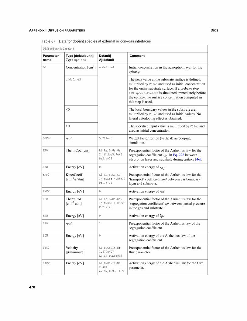
DIOSAPPENDIX I DIFFUSION PARAMETERS
Table 87 Data for dopant species at external silicon–gas interfaces
Diffusion(SiGas(Aj(
Parameter name
Type [default unit]Type Options
Default| Aj:default
Comment
CO Concentration [cm3] undefined Initial concentration in the adsorption layer for the epitaxy.
undefined The peak value at the substrate surface is defined, multiplied by COFac and used as initial concentration for the entire substrate surface. If a prebake step ATMOsphere=Prebake is simulated immediately before the epitaxy, the surface concentration computed in this step is used.
<0 The local boundary values in the substrate are multiplied by COFac and used as initial values. No lateral autodoping effect is obtained.
>0 The specified input value is multiplied by COFac and used as initial concentration.
COFac real 5.714e-5 Weight factor for the (vertical) autodoping simulation.
KA0 ThermCo2 [cm] Al,As,B,Ga,Ge,In,N,Sb:5.7e-5P:2.e-03
Preexponential factor of the Arrhenius law for the segregation coefficient in Eq. 298 between adsorption layer and substrate during epitaxy [46].
KAW Energy [eV] 0 Activation energy of .
KMF0 KinetCoeff [cm–2/s/atm]
Al,As,B,Ga,Ge,In,N,Sb: 4.85e19P:1.e+21
Preexponential factor of the Arrhenius law for the ‘transport’ coefficient kmf between gas boundary layer and substrate.
KMFW Energy [eV] 0 Activation energy of kmf.
KP0 ThermCo1 [cm–3 atm]
Al,As,B,Ga,Ge,In,N,Sb: 1.05e26P:2.e+25
Preexponential factor of the Arrhenius law for the ‘segregation coefficient’ kp between partial pressure in the gas and substrate.
KPW Energy [eV] 0 Activation energy of kp.
SG0 real 1 Preexponential factor of the Arrhenius law of the segregation coefficient.
SGW Energy [eV] 0 Activation energy of the Arrhenius law of the segregation coefficient.
STC0 Velocity [μm/minute]
Al,B,Ga,In,N:1.674e+07As,Ge,P,Sb:9e5
Preexponential factor of the Arrhenius law for the flux parameter.
STCW Energy [eV] Al,B,Ga,In,N:2.481As,Ge,P,Sb: 1.99
Activation energy of the Arrhenius law for the flux parameter.
sg2
sg2
470
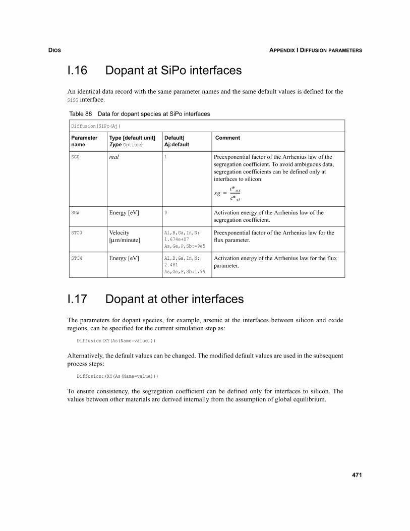
DIOS APPENDIX I DIFFUSION PARAMETERS
I.16 Dopant at SiPo interfacesAn identical data record with the same parameter names and the same default values is defined for theSiSG interface.
I.17 Dopant at other interfacesThe parameters for dopant species, for example, arsenic at the interfaces between silicon and oxideregions, can be specified for the current simulation step as:
Diffusion(XY(As(Name=value)))
Alternatively, the default values can be changed. The modified default values are used in the subsequentprocess steps:
Diffusion:(XY(As(Name=value)))
To ensure consistency, the segregation coefficient can be defined only for interfaces to silicon. Thevalues between other materials are derived internally from the assumption of global equilibrium.
Table 88 Data for dopant species at SiPo interfaces
Diffusion(SiPo(Aj(
Parameter name
Type [default unit]Type Options
Default|Aj:default
Comment
SG0 real 1 Preexponential factor of the Arrhenius law of the segregation coefficient. To avoid ambiguous data, segregation coefficients can be defined only at interfaces to silicon:
SGW Energy [eV] 0 Activation energy of the Arrhenius law of the segregation coefficient.
STC0 Velocity[μm/minute]
Al,B,Ga,In,N:1.674e+07As,Ge,P,Sb:=9e5
Preexponential factor of the Arrhenius law for the flux parameter.
STCW Energy [eV] Al,B,Ga,In,N:2.481As,Ge,P,Sb:1.99
Activation energy of the Arrhenius law for the flux parameter.
sgc∗ox
c∗si----------=
471
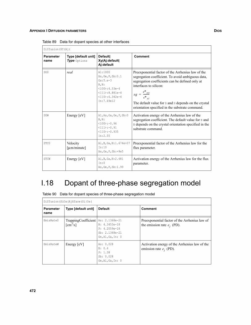
DIOSAPPENDIX I DIFFUSION PARAMETERS
I.18 Dopant of three-phase segregation model
Table 89 Data for dopant species at other interfaces
Diffusion(XY(Aj(
Parameter name
Type [default unit]Type Options
Default|Xy(Aj:default|Aj:default
Comment
SG0 real Al:1000As,Ge,P,Sb:0.1Ga:5.e-3B,N:<100>:4.53e-4<111>:8.881e-4<110>:6.342e-4In:7.69e12
Preexponential factor of the Arrhenius law of the segregation coefficient. To avoid ambiguous data, segregation coefficients can be defined only at interfaces to silicon:
The default value for B and N depends on the crystal orientation specified in the substrate command.
SGW Energy [eV] Al,As,Ga,Ge,P,Sb:0B,N:<100>:-0.96<111>:-0.91<110>:-0.935In:2.55
Activation energy of the Arrhenius law of the segregation coefficient. The default value for B and N depends on the crystal orientation specified in the substrate command.
STC0 Velocity [μm/minute]
Al,B,Ga,N:1.674e+07In:10As,Ge,P,Sb:=9e5
Preexponential factor of the Arrhenius law for the flux parameter.
STCW Energy [eV] Al,B,Ga,N:2.481In:0As,Ge,P,Sb:1.99
Activation energy of the Arrhenius law for the flux parameter.
Table 90 Data for dopant species of three-phase segregation model
Diffusion(SiOx(AjXface(Si|Ox(
Parameter name
Type [default unit] Default Comment
EmisRate0 TrappingCoefficient [cm3/s]
As: 2.1368e-21B: 4.3453e-18P: 4.2059e-18Sb: 2.1368e-21Ge,Al,Ga,In: 0
Preexponential factor of the Arrhenius law of the emission rate (PD).
EmisRateW Energy [eV] As: 0.028B: 0.4P: 1.38Sb: 0.028Ge,Al,Ga,In: 0
Activation energy of the Arrhenius law of the emission rate (PD).
sgc∗ox
c∗si----------=
ej
ej
472
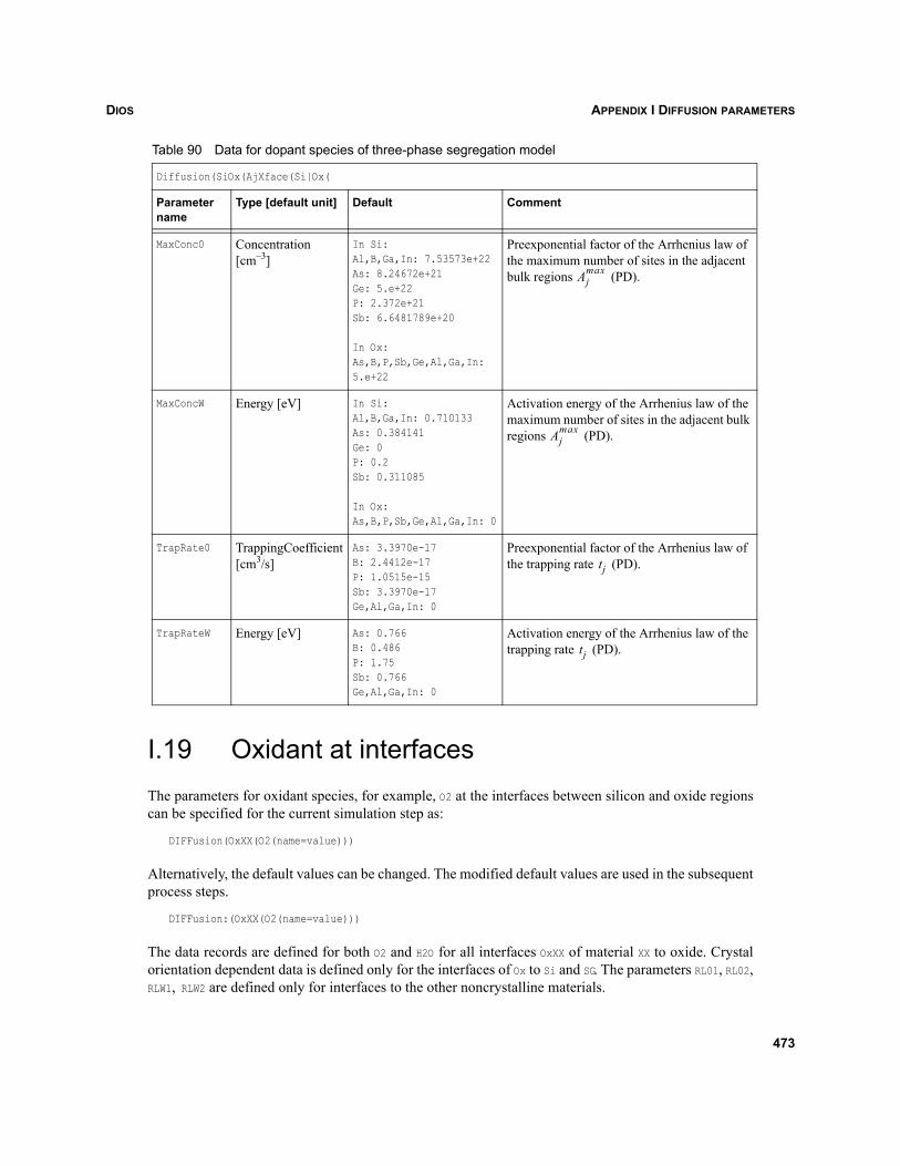
DIOS APPENDIX I DIFFUSION PARAMETERS
I.19 Oxidant at interfacesThe parameters for oxidant species, for example, O2 at the interfaces between silicon and oxide regionscan be specified for the current simulation step as:
DIFFusion(OxXX(O2(name=value)))
Alternatively, the default values can be changed. The modified default values are used in the subsequentprocess steps.
DIFFusion:(OxXX(O2(name=value)))
The data records are defined for both O2 and H2O for all interfaces OxXX of material XX to oxide. Crystalorientation dependent data is defined only for the interfaces of Ox to Si and SG. The parameters RL01, RL02,RLW1, RLW2 are defined only for interfaces to the other noncrystalline materials.
MaxConc0 Concentration [cm–3]
In Si:Al,B,Ga,In: 7.53573e+22As: 8.24672e+21Ge: 5.e+22P: 2.372e+21Sb: 6.6481789e+20
In Ox: As,B,P,Sb,Ge,Al,Ga,In:5.e+22
Preexponential factor of the Arrhenius law of the maximum number of sites in the adjacent bulk regions (PD).
MaxConcW Energy [eV] In Si:Al,B,Ga,In: 0.710133As: 0.384141Ge: 0P: 0.2Sb: 0.311085
In Ox: As,B,P,Sb,Ge,Al,Ga,In: 0
Activation energy of the Arrhenius law of the maximum number of sites in the adjacent bulk regions (PD).
TrapRate0 TrappingCoefficient [cm3/s]
As: 3.3970e-17B: 2.4412e-17P: 1.0515e-15Sb: 3.3970e-17Ge,Al,Ga,In: 0
Preexponential factor of the Arrhenius law of the trapping rate (PD).
TrapRateW Energy [eV] As: 0.766B: 0.486P: 1.75Sb: 0.766Ge,Al,Ga,In: 0
Activation energy of the Arrhenius law of the trapping rate (PD).
Table 90 Data for dopant species of three-phase segregation model
Diffusion(SiOx(AjXface(Si|Ox(
Parameter name
Type [default unit] Default Comment
Ajmax
Ajmax
tj
tj
473
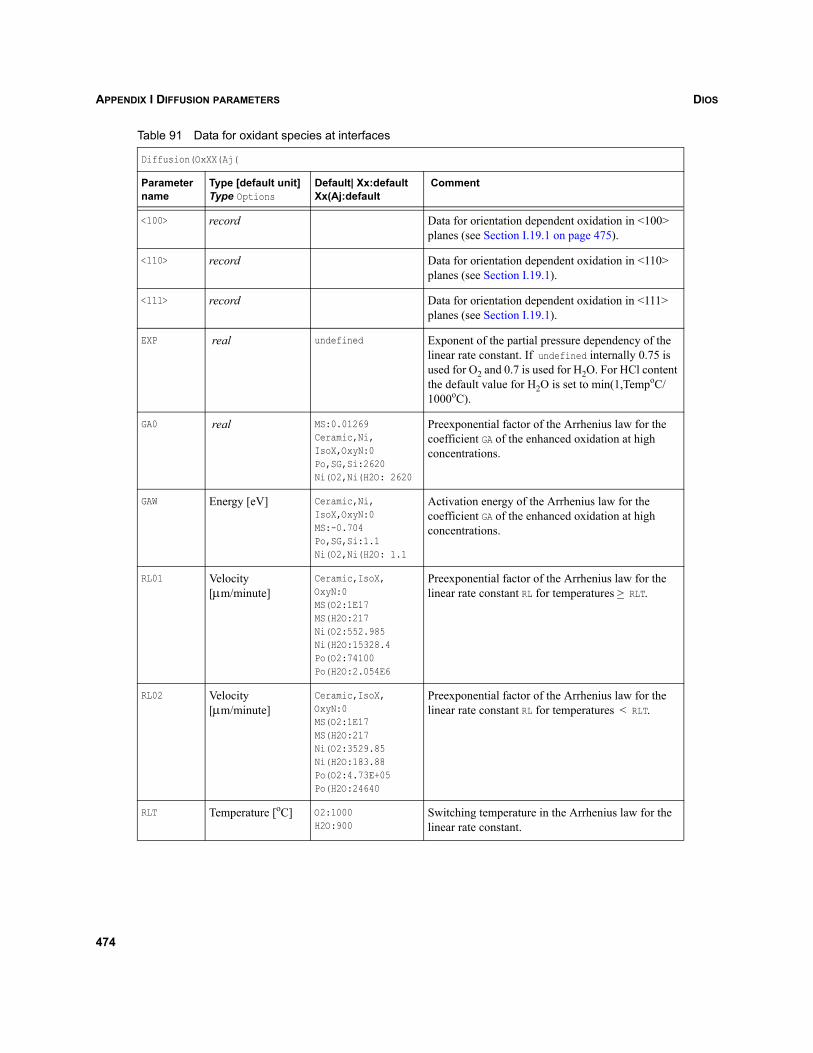
DIOSAPPENDIX I DIFFUSION PARAMETERS
Table 91 Data for oxidant species at interfaces
Diffusion(OxXX(Aj(
Parameter name
Type [default unit]Type Options
Default| Xx:defaultXx(Aj:default
Comment
<100> record Data for orientation dependent oxidation in <100> planes (see Section I.19.1 on page 475).
<110> record Data for orientation dependent oxidation in <110> planes (see Section I.19.1).
<111> record Data for orientation dependent oxidation in <111> planes (see Section I.19.1).
EXP real undefined Exponent of the partial pressure dependency of the linear rate constant. If undefined internally 0.75 is used for O2 and 0.7 is used for H2O. For HCl content the default value for H2O is set to min(1,TempoC/1000oC).
GA0 real MS:0.01269Ceramic,Ni,IsoX,OxyN:0Po,SG,Si:2620Ni(O2,Ni(H2O: 2620
Preexponential factor of the Arrhenius law for the coefficient GA of the enhanced oxidation at high concentrations.
GAW Energy [eV] Ceramic,Ni,IsoX,OxyN:0MS:-0.704Po,SG,Si:1.1Ni(O2,Ni(H2O: 1.1
Activation energy of the Arrhenius law for the coefficient GA of the enhanced oxidation at high concentrations.
RL01 Velocity[μm/minute]
Ceramic,IsoX,OxyN:0MS(O2:1E17MS(H2O:217Ni(O2:552.985Ni(H2O:15328.4Po(O2:74100Po(H2O:2.054E6
Preexponential factor of the Arrhenius law for the linear rate constant RL for temperatures > RLT.
RL02 Velocity[μm/minute]
Ceramic,IsoX,OxyN:0MS(O2:1E17MS(H2O:217Ni(O2:3529.85Ni(H2O:183.88Po(O2:4.73E+05Po(H2O:24640
Preexponential factor of the Arrhenius law for the linear rate constant RL for temperatures < RLT.
RLT Temperature [oC] O2:1000H2O:900
Switching temperature in the Arrhenius law for the linear rate constant.
474
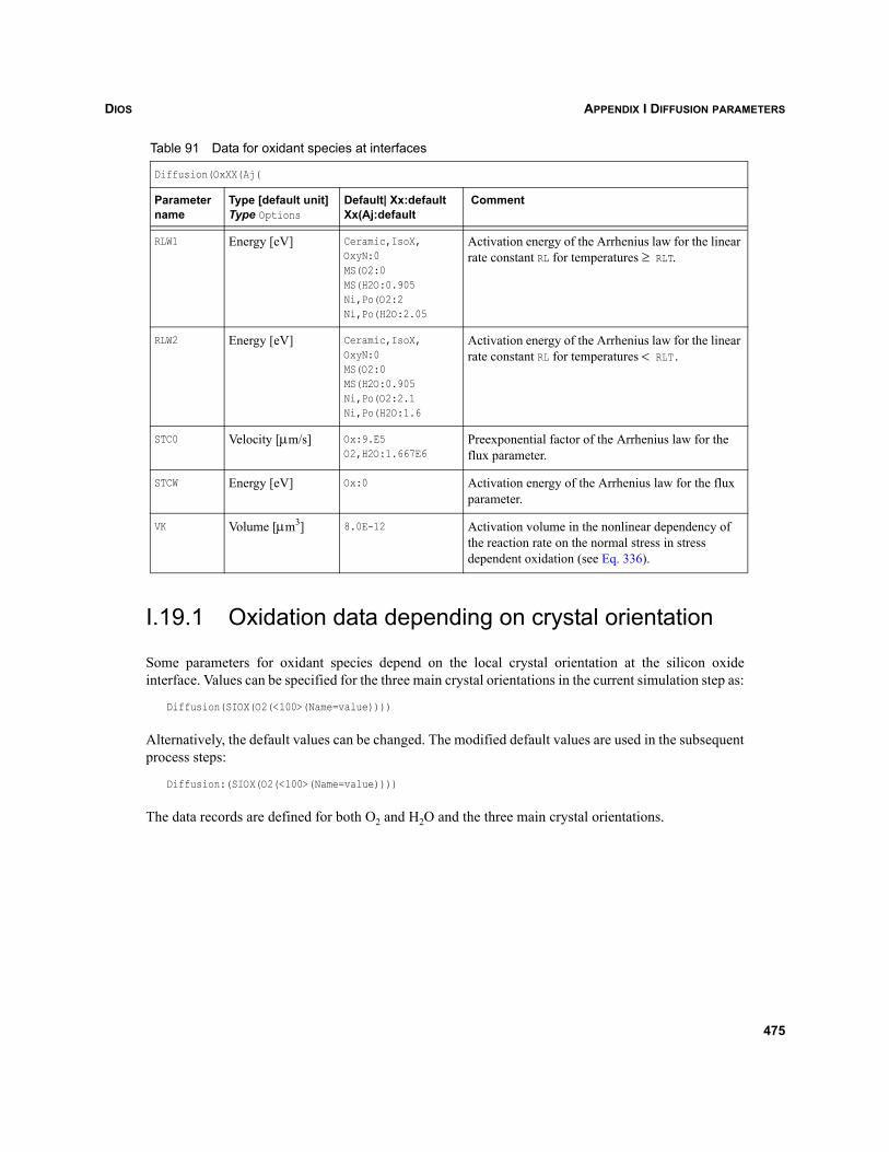
DIOS APPENDIX I DIFFUSION PARAMETERS
I.19.1 Oxidation data depending on crystal orientation
Some parameters for oxidant species depend on the local crystal orientation at the silicon oxideinterface. Values can be specified for the three main crystal orientations in the current simulation step as:
Diffusion(SIOX(O2(<100>(Name=value))))
Alternatively, the default values can be changed. The modified default values are used in the subsequentprocess steps:
Diffusion:(SIOX(O2(<100>(Name=value))))
The data records are defined for both O2 and H2O and the three main crystal orientations.
RLW1 Energy [eV] Ceramic,IsoX,OxyN:0MS(O2:0MS(H2O:0.905Ni,Po(O2:2Ni,Po(H2O:2.05
Activation energy of the Arrhenius law for the linear rate constant RL for temperatures ≥ RLT.
RLW2 Energy [eV] Ceramic,IsoX,OxyN:0MS(O2:0MS(H2O:0.905Ni,Po(O2:2.1Ni,Po(H2O:1.6
Activation energy of the Arrhenius law for the linear rate constant RL for temperatures < RLT.
STC0 Velocity [μm/s] Ox:9.E5O2,H2O:1.667E6
Preexponential factor of the Arrhenius law for the flux parameter.
STCW Energy [eV] Ox:0 Activation energy of the Arrhenius law for the flux parameter.
VK Volume [μm3] 8.0E-12 Activation volume in the nonlinear dependency of the reaction rate on the normal stress in stress dependent oxidation (see Eq. 336).
Table 91 Data for oxidant species at interfaces
Diffusion(OxXX(Aj(
Parameter name
Type [default unit]Type Options
Default| Xx:defaultXx(Aj:default
Comment
475
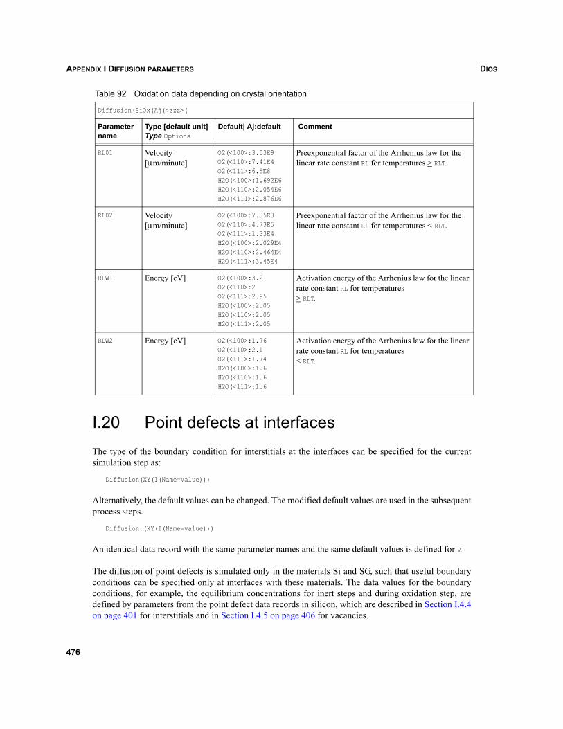
DIOSAPPENDIX I DIFFUSION PARAMETERS
I.20 Point defects at interfacesThe type of the boundary condition for interstitials at the interfaces can be specified for the currentsimulation step as:
Diffusion(XY(I(Name=value)))
Alternatively, the default values can be changed. The modified default values are used in the subsequentprocess steps.
Diffusion:(XY(I(Name=value)))
An identical data record with the same parameter names and the same default values is defined for V.
The diffusion of point defects is simulated only in the materials Si and SG, such that useful boundaryconditions can be specified only at interfaces with these materials. The data values for the boundaryconditions, for example, the equilibrium concentrations for inert steps and during oxidation step, aredefined by parameters from the point defect data records in silicon, which are described in Section I.4.4on page 401 for interstitials and in Section I.4.5 on page 406 for vacancies.
Table 92 Oxidation data depending on crystal orientation
Diffusion(SiOx(Aj(<zzz>(
Parameter name
Type [default unit]Type Options
Default| Aj:default Comment
RL01 Velocity [μm/minute]
O2(<100>:3.53E9O2(<110>:7.41E4O2(<111>:6.5E8H2O(<100>:1.692E6H2O(<110>:2.054E6H2O(<111>:2.876E6
Preexponential factor of the Arrhenius law for the linear rate constant RL for temperatures > RLT.
RL02 Velocity [μm/minute]
O2(<100>:7.35E3O2(<110>:4.73E5O2(<111>:1.33E4H2O(<100>:2.029E4H2O(<110>:2.464E4H2O(<111>:3.45E4
Preexponential factor of the Arrhenius law for the linear rate constant RL for temperatures < RLT.
RLW1 Energy [eV] O2(<100>:3.2O2(<110>:2O2(<111>:2.95H2O(<100>:2.05H2O(<110>:2.05H2O(<111>:2.05
Activation energy of the Arrhenius law for the linear rate constant RL for temperatures > RLT.
RLW2 Energy [eV] O2(<100>:1.76O2(<110>:2.1O2(<111>:1.74H2O(<100>:1.6H2O(<110>:1.6H2O(<111>:1.6
Activation energy of the Arrhenius law for the linear rate constant RL for temperatures < RLT.
476
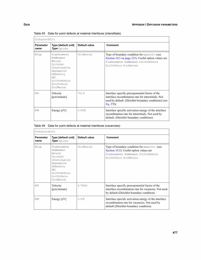
DIOS APPENDIX I DIFFUSION PARAMETERS
Table 93 Data for point defects at material interfaces (interstitials)
Diffusion(XY(I(
Parameter name
Type [default unit]Type Options
Default value Comment
BCtyp FluxParameterHomNeumannNaturalDirichlet1DcontinuationSegregation SURDensity GBC DiriTotNoPairsDiriTotPairsDiriNeutral
DiriNeutral Type of boundary condition for NewDiff=1 (see Section 10.5 on page 223). Useful option values are FluxParameter HomNeumann DiriTotNoPairs DiriTotPairs DiriNeutral.
KS0 Velocity [μm/minute]
722.4 Interface specific preexponential factor of the interface recombination rate for interstitials. Not used by default. (Dirichlet boundary conditions) (see Eq. 270).
KSW Energy [eV] 0.4392 Interface specific activation energy of the interface recombination rate for interstitials. Not used by default. (Dirichlet boundary conditions).
Table 94 Data for point defects at material interfaces (vacancies)
Diffusion(XY(V(
Parameter name
Type [default unit]Type Options
Default value Comment
BCtyp FluxParameterHomNeumannNaturalDirichlet1DcontinuationSegregation SURDensity GBC DiriTotNoPairsDiriTotPairsDiriNeutral
DiriNeutral Type of boundary condition for NewDiff=1 (see Section 10.5). Useful option values are FluxParameter HomNeumann DiriTotNoPairs DiriTotPairs DiriNeutral.
KS0 Velocity[μm/minute]
6.702e9 Interface specific preexponential factor of the interface recombination rate for vacancies. Not used by default (Dirichlet boundary condition).
KSW Energy [eV] 2.478 Interface specific activation energy of the interface recombination rate for vacancies. Not used by default (Dirichlet boundary condition).
477
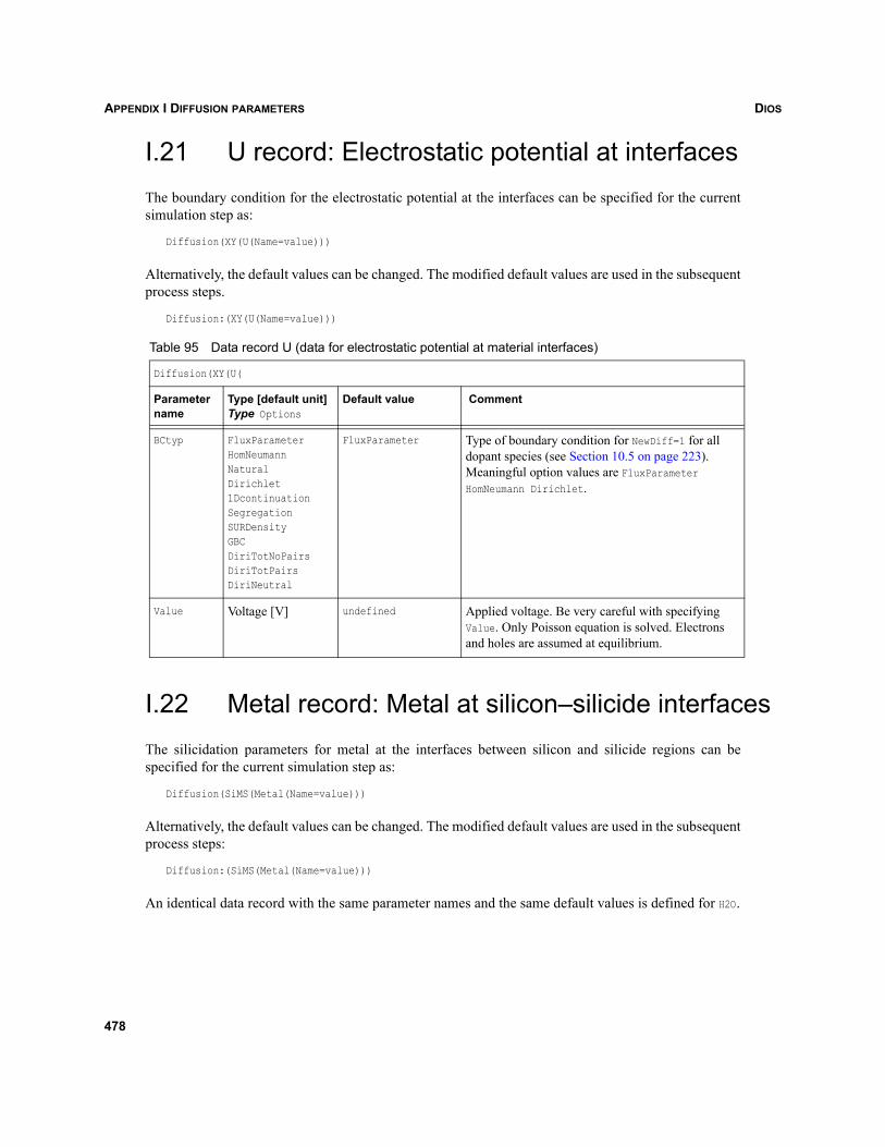
DIOSAPPENDIX I DIFFUSION PARAMETERS
I.21 U record: Electrostatic potential at interfacesThe boundary condition for the electrostatic potential at the interfaces can be specified for the currentsimulation step as:
Diffusion(XY(U(Name=value)))
Alternatively, the default values can be changed. The modified default values are used in the subsequentprocess steps.
Diffusion:(XY(U(Name=value)))
I.22 Metal record: Metal at silicon–silicide interfacesThe silicidation parameters for metal at the interfaces between silicon and silicide regions can bespecified for the current simulation step as:
Diffusion(SiMS(Metal(Name=value)))
Alternatively, the default values can be changed. The modified default values are used in the subsequentprocess steps:
Diffusion:(SiMS(Metal(Name=value)))
An identical data record with the same parameter names and the same default values is defined for H2O.
Table 95 Data record U (data for electrostatic potential at material interfaces)
Diffusion(XY(U(
Parameter name
Type [default unit]Type Options
Default value Comment
BCtyp FluxParameterHomNeumannNaturalDirichlet1DcontinuationSegregation SURDensity GBC DiriTotNoPairsDiriTotPairsDiriNeutral
FluxParameter Type of boundary condition for NewDiff=1 for all dopant species (see Section 10.5 on page 223). Meaningful option values are FluxParameter HomNeumann Dirichlet.
Value Voltage [V] undefined Applied voltage. Be very careful with specifying Value. Only Poisson equation is solved. Electrons and holes are assumed at equilibrium.
478
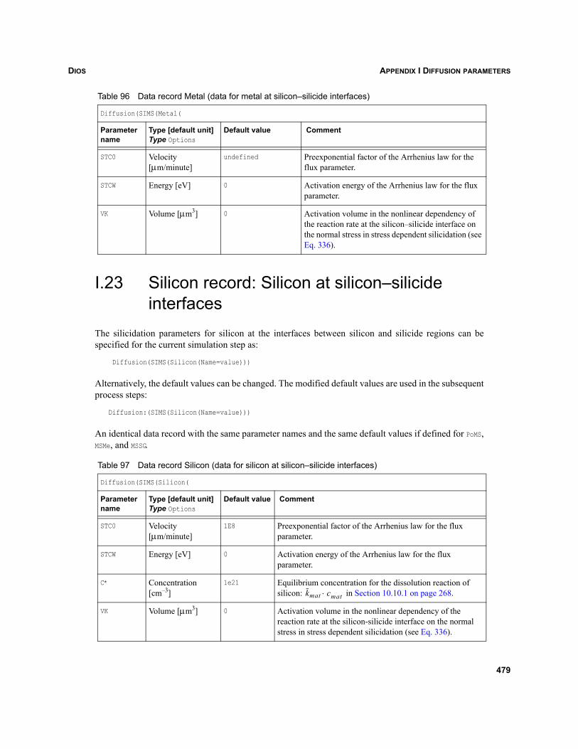
DIOS APPENDIX I DIFFUSION PARAMETERS
I.23 Silicon record: Silicon at silicon–silicide interfaces
The silicidation parameters for silicon at the interfaces between silicon and silicide regions can bespecified for the current simulation step as:
Diffusion(SIMS(Silicon(Name=value)))
Alternatively, the default values can be changed. The modified default values are used in the subsequentprocess steps:
Diffusion:(SIMS(Silicon(Name=value)))
An identical data record with the same parameter names and the same default values if defined for PoMS,MSMe, and MSSG.
Table 96 Data record Metal (data for metal at silicon–silicide interfaces)
Diffusion(SIMS(Metal(
Parameter name
Type [default unit]Type Options
Default value Comment
STC0 Velocity[μm/minute]
undefined Preexponential factor of the Arrhenius law for the flux parameter.
STCW Energy [eV] 0 Activation energy of the Arrhenius law for the flux parameter.
VK Volume [μm3] 0 Activation volume in the nonlinear dependency of the reaction rate at the silicon–silicide interface on the normal stress in stress dependent silicidation (see Eq. 336).
Table 97 Data record Silicon (data for silicon at silicon–silicide interfaces)
Diffusion(SIMS(Silicon(
Parameter name
Type [default unit]Type Options
Default value Comment
STC0 Velocity[μm/minute]
1E8 Preexponential factor of the Arrhenius law for the flux parameter.
STCW Energy [eV] 0 Activation energy of the Arrhenius law for the flux parameter.
C* Concentration [cm–3]
1e21 Equilibrium concentration for the dissolution reaction of silicon: in Section 10.10.1 on page 268.
VK Volume [μm3] 0 Activation volume in the nonlinear dependency of the reaction rate at the silicon-silicide interface on the normal stress in stress dependent silicidation (see Eq. 336).
kmat cmat⋅
479
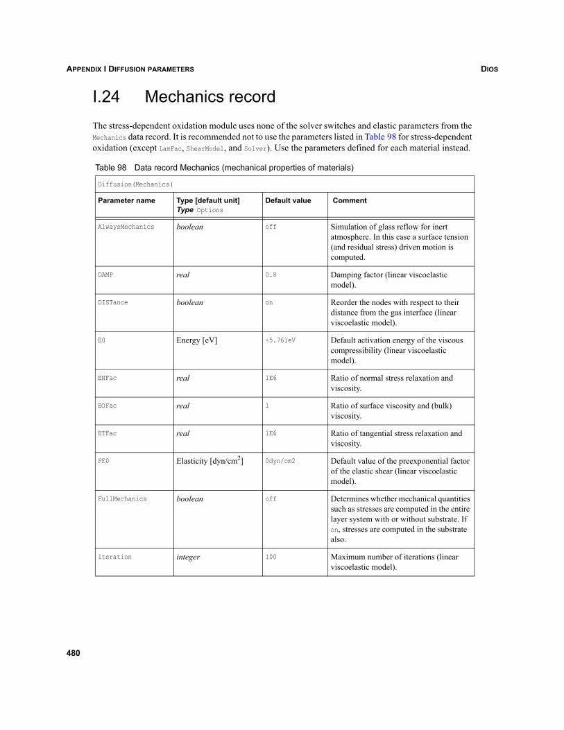
DIOSAPPENDIX I DIFFUSION PARAMETERS
I.24 Mechanics recordThe stress-dependent oxidation module uses none of the solver switches and elastic parameters from theMechanics data record. It is recommended not to use the parameters listed in Table 98 for stress-dependentoxidation (except LamFac, ShearModel, and Solver). Use the parameters defined for each material instead.
Table 98 Data record Mechanics (mechanical properties of materials)
Diffusion(Mechanics(
Parameter name Type [default unit]Type Options
Default value Comment
AlwaysMechanics boolean off Simulation of glass reflow for inert atmosphere. In this case a surface tension (and residual stress) driven motion is computed.
DAMP real 0.8 Damping factor (linear viscoelastic model).
DISTance boolean on Reorder the nodes with respect to their distance from the gas interface (linear viscoelastic model).
E0 Energy [eV] -5.761eV Default activation energy of the viscous compressibility (linear viscoelastic model).
ENFac real 1E6 Ratio of normal stress relaxation and viscosity.
EOFac real 1 Ratio of surface viscosity and (bulk) viscosity.
ETFac real 1E6 Ratio of tangential stress relaxation and viscosity.
FE0 Elasticity [dyn/cm2] 0dyn/cm2 Default value of the preexponential factor of the elastic shear (linear viscoelastic model).
FullMechanics boolean off Determines whether mechanical quantities such as stresses are computed in the entire layer system with or without substrate. If on, stresses are computed in the substrate also.
Iteration integer 100 Maximum number of iterations (linear viscoelastic model).
480
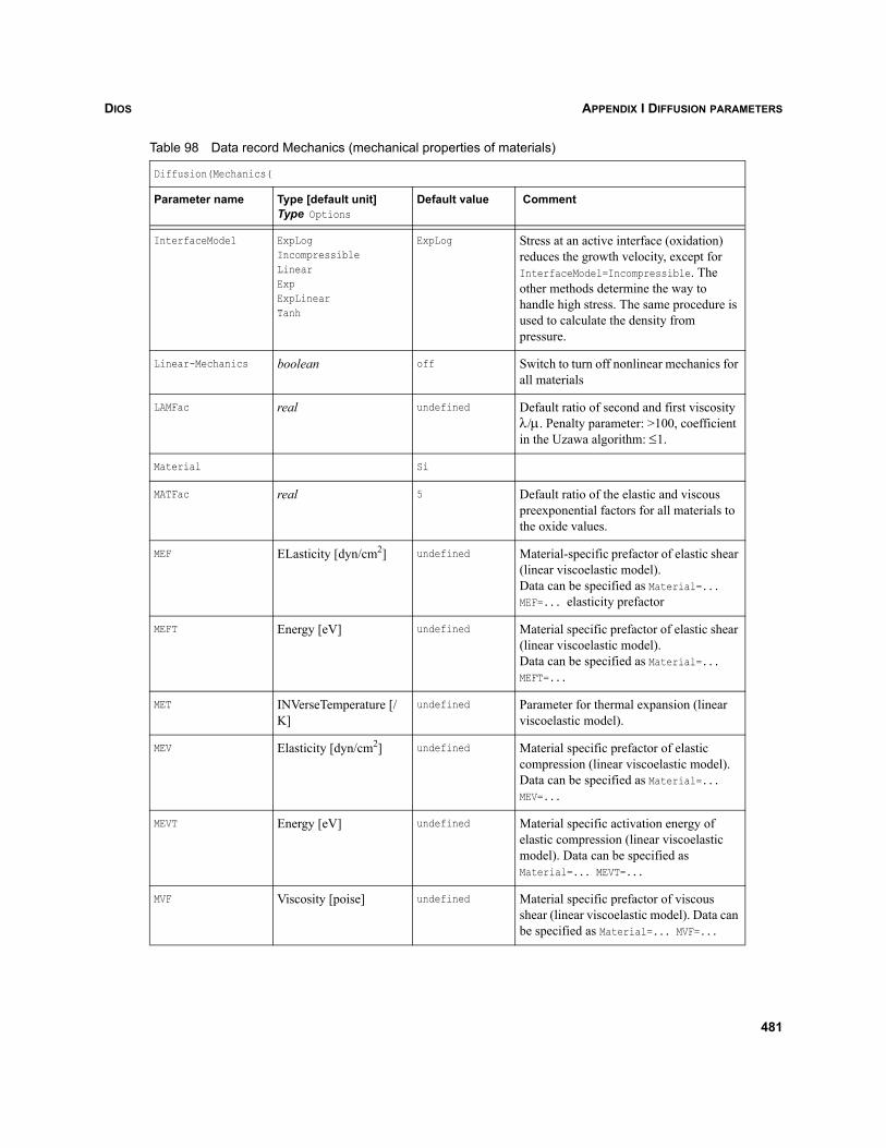
DIOS APPENDIX I DIFFUSION PARAMETERS
InterfaceModel ExpLogIncompressibleLinearExpExpLinearTanh
ExpLog Stress at an active interface (oxidation) reduces the growth velocity, except for InterfaceModel=Incompressible. The other methods determine the way to handle high stress. The same procedure is used to calculate the density from pressure.
Linear-Mechanics boolean off Switch to turn off nonlinear mechanics for all materials
LAMFac real undefined Default ratio of second and first viscosity λ/μ. Penalty parameter: >100, coefficient in the Uzawa algorithm: ≤1.
Material Si
MATFac real 5 Default ratio of the elastic and viscous preexponential factors for all materials to the oxide values.
MEF ELasticity [dyn/cm2] undefined Material-specific prefactor of elastic shear (linear viscoelastic model). Data can be specified as Material=... MEF=... elasticity prefactor
MEFT Energy [eV] undefined Material specific prefactor of elastic shear (linear viscoelastic model).Data can be specified as Material=... MEFT=...
MET INVerseTemperature [/K]
undefined Parameter for thermal expansion (linear viscoelastic model).
MEV Elasticity [dyn/cm2] undefined Material specific prefactor of elastic compression (linear viscoelastic model). Data can be specified as Material=... MEV=...
MEVT Energy [eV] undefined Material specific activation energy of elastic compression (linear viscoelastic model). Data can be specified as Material=... MEVT=...
MVF Viscosity [poise] undefined Material specific prefactor of viscous shear (linear viscoelastic model). Data can be specified as Material=... MVF=...
Table 98 Data record Mechanics (mechanical properties of materials)
Diffusion(Mechanics(
Parameter name Type [default unit]Type Options
Default value Comment
481
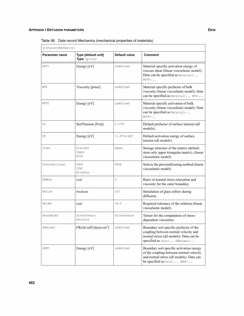
DIOSAPPENDIX I DIFFUSION PARAMETERS
MVFT Energy [eV] undefined Material specific activation energy of viscous shear (linear viscoelastic model). Data can be specified as Material=... MVFT=...
MVV Viscosity [poise] undefined Material specific prefactor of bulk viscosity (linear viscoelastic model). Data can be specified as Material=... MVV=...
MVVT Energy [eV] undefined Material specific activation of bulk viscosity (linear viscoelastic model). Data can be specified as Material=... MVVT=...
O0 SurfTension [N/m] 0.2791 Default prefactor of surface tension (all models).
OE Energy [eV] -1.837e-2eV Default activation energy of surface tension (all models).
Order DisorderUpperBoth
Upper Storage structure of the matrix (default: store only upper triangular matrix). (linear viscoelastic model).
Preconditioner SSORIFACBlockfac
SSOR Selects the preconditioning method (linear viscoelastic model).
RANFac real 0 Ratio of normal stress relaxation and viscosity for the outer boundary.
Reflow boolean off Simulation of glass reflow during diffusion.
Reldef real 1E-4 Required tolerance of the solution (linear viscoelastic model).
ShearModel StressTensorDeviator
StressTensor Tensor for the computation of stress-dependent viscosities.
SHNormal FRictCoeff [dyns/cm3] undefined Boundary sort specific prefactor of the coupling between normal velocity and normal stress (all models). Data can be specified as Sort=... SHNormal=...
SHNT Energy [eV] undefined Boundary sort specific activation energy of the coupling between normal velocity and normal stress (all models). Data can be specified as Sort=... SHNT=...
Table 98 Data record Mechanics (mechanical properties of materials)
Diffusion(Mechanics(
Parameter name Type [default unit]Type Options
Default value Comment
482
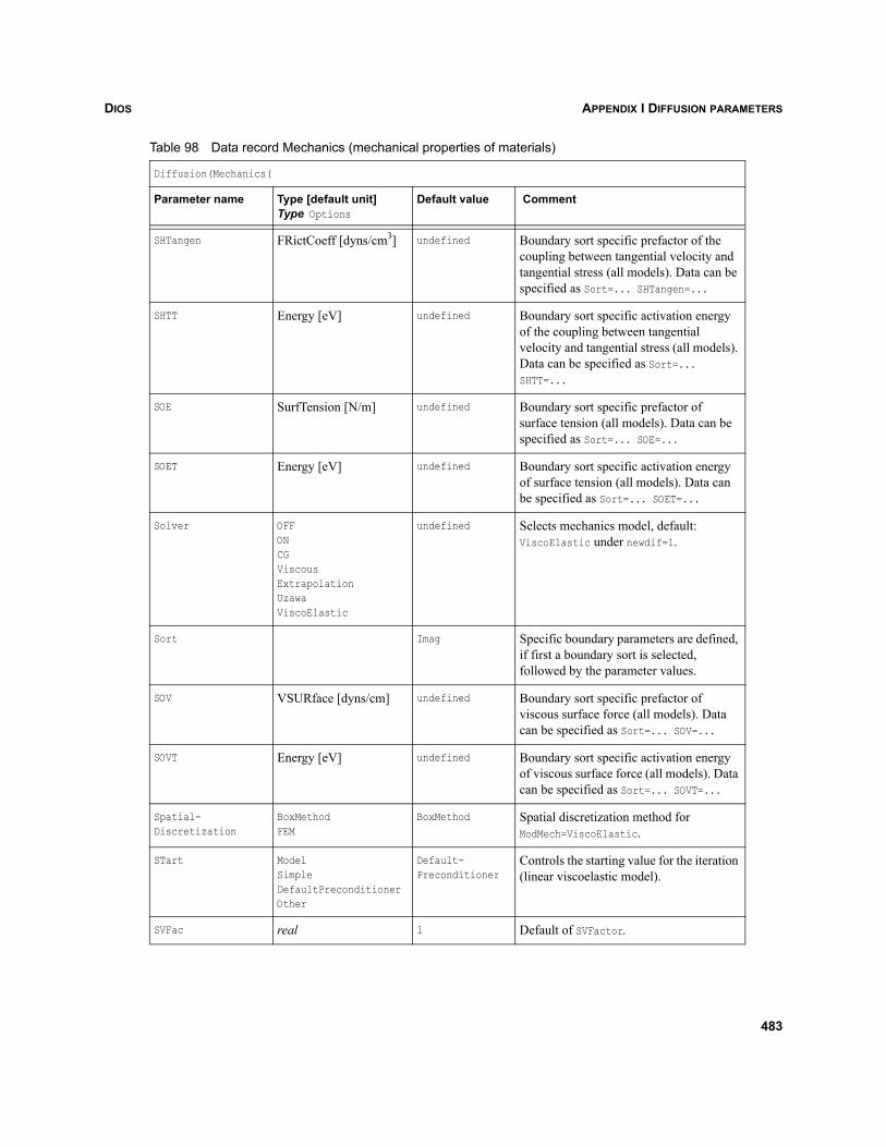
DIOS APPENDIX I DIFFUSION PARAMETERS
SHTangen FRictCoeff [dyns/cm3] undefined Boundary sort specific prefactor of the coupling between tangential velocity and tangential stress (all models). Data can be specified as Sort=... SHTangen=...
SHTT Energy [eV] undefined Boundary sort specific activation energy of the coupling between tangential velocity and tangential stress (all models). Data can be specified as Sort=... SHTT=...
SOE SurfTension [N/m] undefined Boundary sort specific prefactor of surface tension (all models). Data can be specified as Sort=... SOE=...
SOET Energy [eV] undefined Boundary sort specific activation energy of surface tension (all models). Data can be specified as Sort=... SOET=...
Solver OFFONCGViscousExtrapolationUzawaViscoElastic
undefined Selects mechanics model, default: ViscoElastic under newdif=1.
Sort Imag Specific boundary parameters are defined, if first a boundary sort is selected, followed by the parameter values.
SOV VSURface [dyns/cm] undefined Boundary sort specific prefactor of viscous surface force (all models). Data can be specified as Sort=... SOV=...
SOVT Energy [eV] undefined Boundary sort specific activation energy of viscous surface force (all models). Data can be specified as Sort=... SOVT=...
Spatial-Discretization
BoxMethodFEM
BoxMethod Spatial discretization method for ModMech=ViscoElastic.
STart ModelSimpleDefaultPreconditionerOther
Default-Preconditioner
Controls the starting value for the iteration (linear viscoelastic model).
SVFac real 1 Default of SVFactor.
Table 98 Data record Mechanics (mechanical properties of materials)
Diffusion(Mechanics(
Parameter name Type [default unit]Type Options
Default value Comment
483
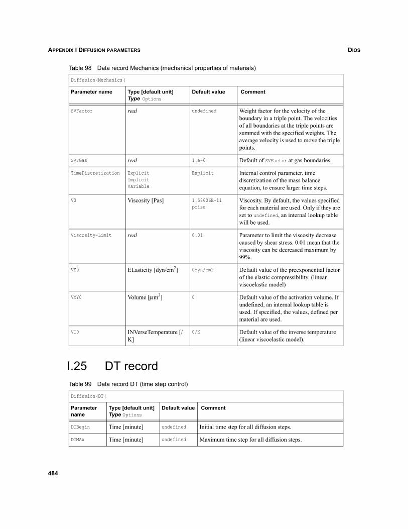
DIOSAPPENDIX I DIFFUSION PARAMETERS
I.25 DT record
SVFactor real undefined Weight factor for the velocity of the boundary in a triple point. The velocities of all boundaries at the triple points are summed with the specified weights. The average velocity is used to move the triple points.
SVFGas real 1.e-6 Default of SVFactor at gas boundaries.
TimeDiscretization ExplicitImplicitVariable
Explicit Internal control parameter. time discretization of the mass balance equation, to ensure larger time steps.
V0 Viscosity [Pas] 1.58606E-11 poise
Viscosity. By default, the values specified for each material are used. Only if they are set to undefined, an internal lookup table will be used.
Viscosity-Limit real 0.01 Parameter to limit the viscosity decrease caused by shear stress. 0.01 mean that the viscosity can be decreased maximum by 99%.
VE0 ELasticity [dyn/cm2] 0dyn/cm2 Default value of the preexponential factor of the elastic compressibility. (linear viscoelastic model)
VMY0 Volume [μm3] 0 Default value of the activation volume. If undefined, an internal lookup table is used. If specified, the values, defined per material are used.
VT0 INVerseTemperature [/K]
0/K Default value of the inverse temperature (linear viscoelastic model).
Table 99 Data record DT (time step control)
Diffusion(DT(
Parameter name
Type [default unit]Type Options
Default value Comment
DTBegin Time [minute] undefined Initial time step for all diffusion steps.
DTMAx Time [minute] undefined Maximum time step for all diffusion steps.
Table 98 Data record Mechanics (mechanical properties of materials)
Diffusion(Mechanics(
Parameter name Type [default unit]Type Options
Default value Comment
484
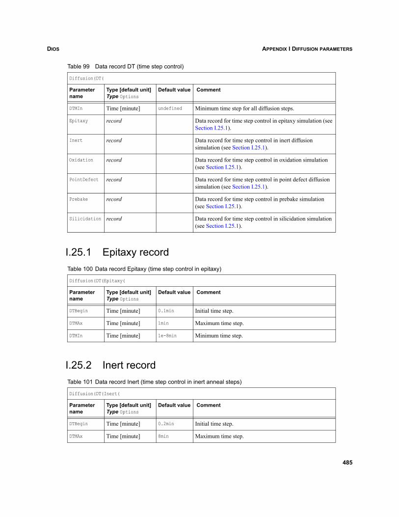
DIOS APPENDIX I DIFFUSION PARAMETERS
I.25.1 Epitaxy record
I.25.2 Inert record
DTMIn Time [minute] undefined Minimum time step for all diffusion steps.
Epitaxy record Data record for time step control in epitaxy simulation (see Section I.25.1).
Inert record Data record for time step control in inert diffusion simulation (see Section I.25.1).
Oxidation record Data record for time step control in oxidation simulation (see Section I.25.1).
PointDefect record Data record for time step control in point defect diffusion simulation (see Section I.25.1).
Prebake record Data record for time step control in prebake simulation (see Section I.25.1).
Silicidation record Data record for time step control in silicidation simulation (see Section I.25.1).
Table 100 Data record Epitaxy (time step control in epitaxy)
Diffusion(DT(Epitaxy(
Parameter name
Type [default unit]Type Options
Default value Comment
DTBegin Time [minute] 0.1min Initial time step.
DTMAx Time [minute] 1min Maximum time step.
DTMIn Time [minute] 1e-8min Minimum time step.
Table 101 Data record Inert (time step control in inert anneal steps)
Diffusion(DT(Inert(
Parameter name
Type [default unit]Type Options
Default value Comment
DTBegin Time [minute] 0.2min Initial time step.
DTMAx Time [minute] 8min Maximum time step.
Table 99 Data record DT (time step control)
Diffusion(DT(
Parameter name
Type [default unit]Type Options
Default value Comment
485
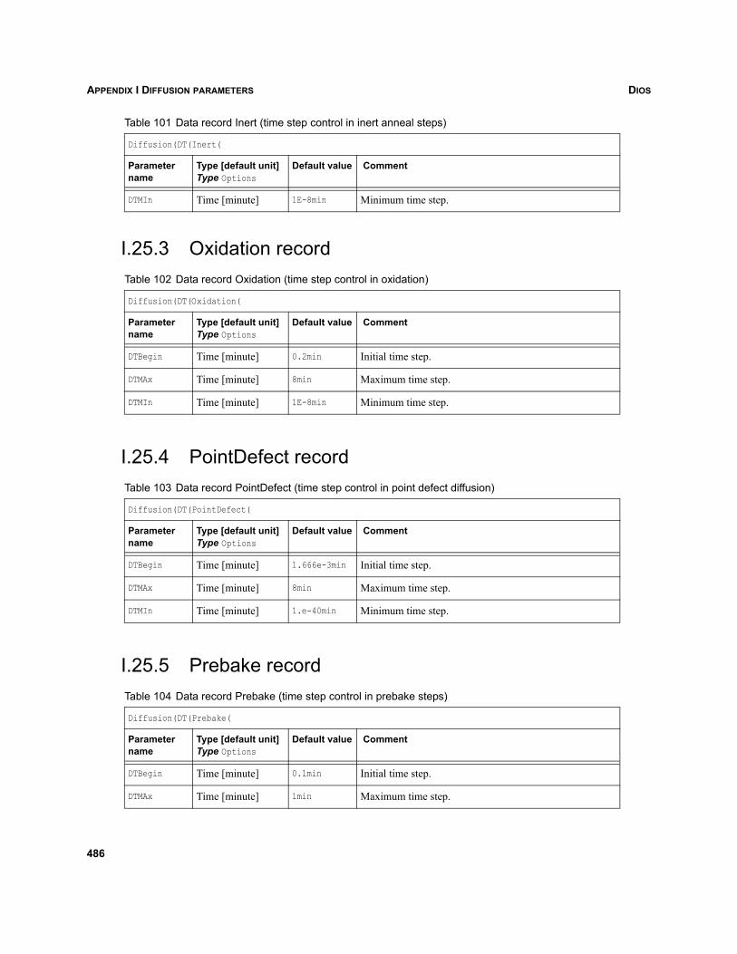
DIOSAPPENDIX I DIFFUSION PARAMETERS
I.25.3 Oxidation record
I.25.4 PointDefect record
I.25.5 Prebake record
DTMIn Time [minute] 1E-8min Minimum time step.
Table 102 Data record Oxidation (time step control in oxidation)
Diffusion(DT(Oxidation(
Parameter name
Type [default unit]Type Options
Default value Comment
DTBegin Time [minute] 0.2min Initial time step.
DTMAx Time [minute] 8min Maximum time step.
DTMIn Time [minute] 1E-8min Minimum time step.
Table 103 Data record PointDefect (time step control in point defect diffusion)
Diffusion(DT(PointDefect(
Parameter name
Type [default unit]Type Options
Default value Comment
DTBegin Time [minute] 1.666e-3min Initial time step.
DTMAx Time [minute] 8min Maximum time step.
DTMIn Time [minute] 1.e-40min Minimum time step.
Table 104 Data record Prebake (time step control in prebake steps)
Diffusion(DT(Prebake(
Parameter name
Type [default unit]Type Options
Default value Comment
DTBegin Time [minute] 0.1min Initial time step.
DTMAx Time [minute] 1min Maximum time step.
Table 101 Data record Inert (time step control in inert anneal steps)
Diffusion(DT(Inert(
Parameter name
Type [default unit]Type Options
Default value Comment
486
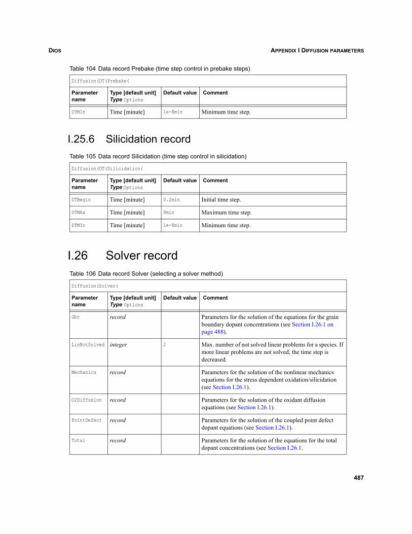
DIOS APPENDIX I DIFFUSION PARAMETERS
I.25.6 Silicidation record
I.26 Solver record
DTMIn Time [minute] 1e-8min Minimum time step.
Table 105 Data record Silicidation (time step control in silicidation)
Diffusion(DT(Silicidation(
Parameter name
Type [default unit]Type Options
Default value Comment
DTBegin Time [minute] 0.2min Initial time step.
DTMAx Time [minute] 8min Maximum time step.
DTMIn Time [minute] 1e-8min Minimum time step.
Table 106 Data record Solver (selecting a solver method)
Diffusion(Solver(
Parameter name
Type [default unit]Type Options
Default value Comment
Gbc record Parameters for the solution of the equations for the grain boundary dopant concentrations (see Section I.26.1 on page 488).
LinNotSolved integer 2 Max. number of not solved linear problems for a species. If more linear problems are not solved, the time step is decreased.
Mechanics record Parameters for the solution of the nonlinear mechanics equations for the stress dependent oxidation/silicidation (see Section I.26.1).
O2Diffusion record Parameters for the solution of the oxidant diffusion equations (see Section I.26.1).
PointDefect record Parameters for the solution of the coupled point defect dopant equations (see Section I.26.1).
Total record Parameters for the solution of the equations for the total dopant concentrations (see Section I.26.1.
Table 104 Data record Prebake (time step control in prebake steps)
Diffusion(DT(Prebake(
Parameter name
Type [default unit]Type Options
Default value Comment
487

DIOSAPPENDIX I DIFFUSION PARAMETERS
I.26.1 Total record
Similar records exist for Gbc, O2Diffusion, and Mechanics. In the column with the default value, theappropriate record names are listed, followed by a colon and the default value. A dash indicates that theparameter is not defined in the corresponding record. The data for the PointDefect solver are listed inSection I.26.2 on page 493. The linear viscoelastic problem is solved according to the solver selectionin Section I.24 on page 480.
The parameters listed in Table 107 on page 488 as far as they concern Mechanics are used only for thestress-dependent oxidation (that is, the Uzawa and viscous models).
Table 107 Data record Total (selecting the solver for the total concentrations)
Diffusion(Solver(Total(
Parameter name Type [default unit]Type Options
Default value Comment
Damping record 0.5 Damping factor (not used). Parameter can be specified per dopant species from the appropriate group:gbc: AlGbc, AsGbc, BGbc, GaGbc, GeGbc, InGbc, NGbc, PGbc, SbGbc;total: AlTotal, AsTotal, BTotal, GaTotal, GeTotal, InTotal, NTotal, PTotal, SbTotal;o2diffusion: H2oTotal, OTotalmechanics: Only one real number
DEFA real Mechanics: 81others:8100
Required defect reduction for the solution of linear systems. If the defect reduction is insufficient, the linear system is treated as not solved and the time step is reduced.
DEFLin real Mechanics: 0.01others:1e-4
Required defect reduction in the iterative linear solver.
488
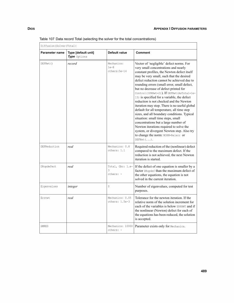
DIOS APPENDIX I DIFFUSION PARAMETERS
DEFNwt() record Mechanics:1e-8others:5e-14
Vector of ‘negligible’ defect norms. For very small concentrations and nearly constant profiles, the Newton defect itself may be very small, such that the desired defect reduction cannot be achieved due to rounding errors (small error, small defect, but no decrease of defect printed for Control(IPRNwt=2)). If DEFNwt(AsTotal=1e-15) is specified for a variable, the defect reduction is not checked and the Newton iteration may stop. There is no useful global default for all temperature, all time step sizes, and all boundary conditions. Typical situation: small time steps, small concentrations but a large number of Newton iterations required to solve the system, or divergent Newton step. Also try to change the norm: NORM=Relerr or DEFNwt(...).
DEFReduction real Mechanics: 0.8others: 1.1
Required reduction of the (nonlinear) defect compared to the maximum defect. If the reduction is not achieved, the next Newton iteration is started.
DRopdefect real Total, Gbc: 1.e-3others: -
If the defect of one equation is smaller by a factor DRopdef than the maximum defect of the other equations, the equation is not solved in the current iteration.
Eigenvalues integer 0 Number of eigenvalues, computed for test purposes.
Errnwt real Mechanics: 0.05others: 1.5e-3
Tolerance for the newton iteration. If the relative norm of the solution increment for each of the variables is below ERRNWT and if the nonlinear (Newton) defect for each of the equations has been reduced, the solution is accepted.
GMRES Mechanics: 10000others: -
Parameter exists only for Mechanics.
Table 107 Data record Total (selecting the solver for the total concentrations)
Diffusion(Solver(Total(
Parameter name Type [default unit]Type Options
Default value Comment
489
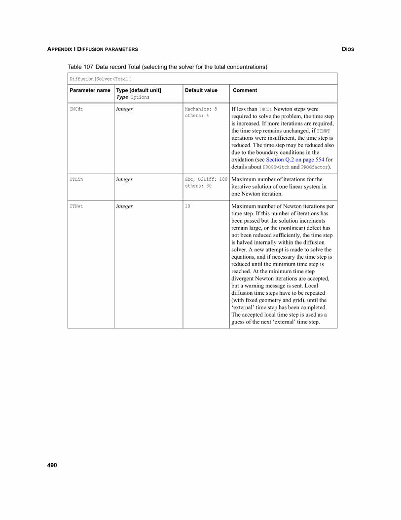
DIOSAPPENDIX I DIFFUSION PARAMETERS
INCdt integer Mechanics: 8others: 4
If less than INCdt Newton steps were required to solve the problem, the time step is increased. If more iterations are required, the time step remains unchanged, if ITNWT iterations were insufficient, the time step is reduced. The time step may be reduced also due to the boundary conditions in the oxidation (see Section Q.2 on page 554 for details about PROGSwitch and PROGfactor).
ITLin integer Gbc, O2Diff: 100others: 30
Maximum number of iterations for the iterative solution of one linear system in one Newton iteration.
ITNwt integer 10 Maximum number of Newton iterations per time step. If this number of iterations has been passed but the solution increments remain large, or the (nonlinear) defect has not been reduced sufficiently, the time step is halved internally within the diffusion solver. A new attempt is made to solve the equations, and if necessary the time step is reduced until the minimum time step is reached. At the minimum time step divergent Newton iterations are accepted, but a warning message is sent. Local diffusion time steps have to be repeated (with fixed geometry and grid), until the ‘external’ time step has been completed. The accepted local time step is used as a guess of the next ‘external’ time step.
Table 107 Data record Total (selecting the solver for the total concentrations)
Diffusion(Solver(Total(
Parameter name Type [default unit]Type Options
Default value Comment
490
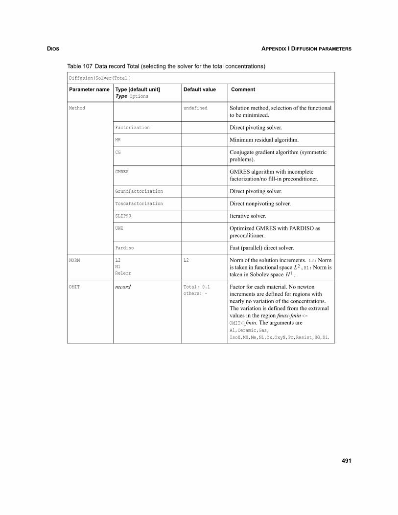
DIOS APPENDIX I DIFFUSION PARAMETERS
Method undefined Solution method, selection of the functional to be minimized.
Factorization Direct pivoting solver.
MR Minimum residual algorithm.
CG Conjugate gradient algorithm (symmetric problems).
GMRES GMRES algorithm with incomplete factorization/no fill-in preconditioner.
GrundFactorization Direct pivoting solver.
ToscaFactorization Direct nonpivoting solver.
SLIP90 Iterative solver.
UWE Optimized GMRES with PARDISO as preconditioner.
Pardiso Fast (parallel) direct solver.
NORM L2H1Relerr
L2 Norm of the solution increments. L2: Norm is taken in functional space , H1: Norm is taken in Sobolev space .
OMIT record Total: 0.1others: -
Factor for each material. No newton increments are defined for regions with nearly no variation of the concentrations. The variation is defined from the extremal values in the region fmax-fmin <= OMIT()fmin. The arguments are Al,Ceramic,Gas, IsoX,MS,Me,Ni,Ox,OxyN,Po,Resist,SG,Si.
Table 107 Data record Total (selecting the solver for the total concentrations)
Diffusion(Solver(Total(
Parameter name Type [default unit]Type Options
Default value Comment
L2
H1
491
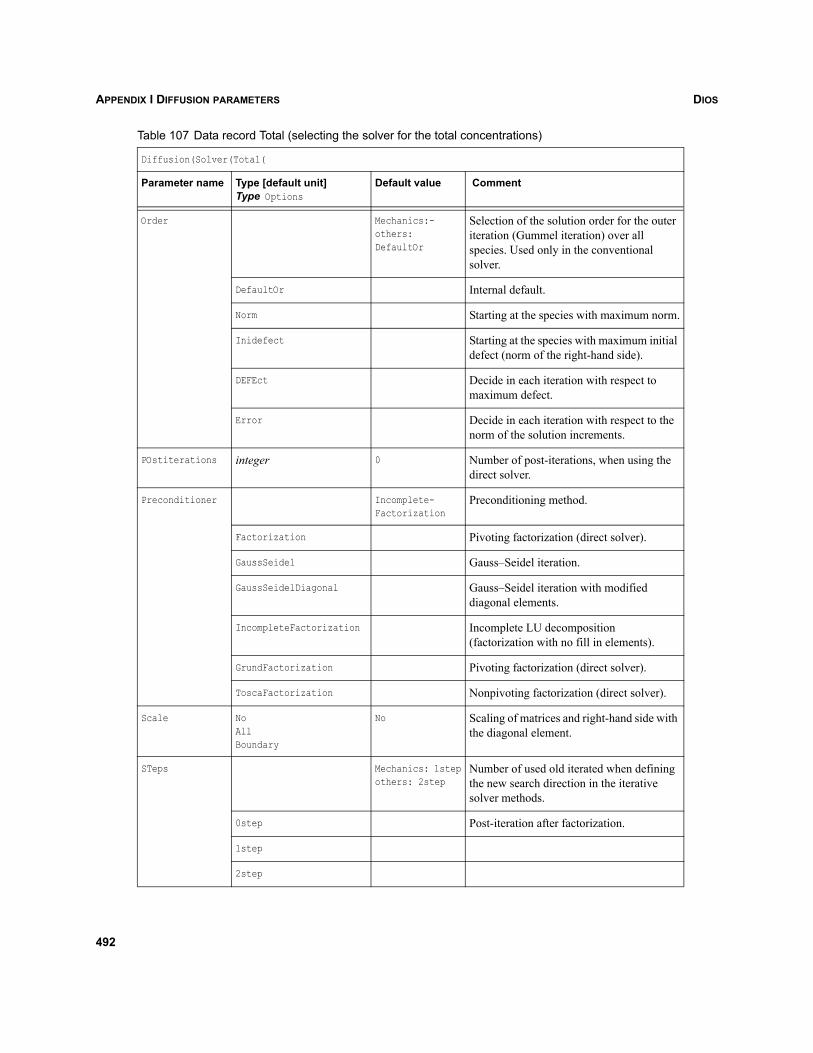
DIOSAPPENDIX I DIFFUSION PARAMETERS
Order Mechanics:-others: DefaultOr
Selection of the solution order for the outer iteration (Gummel iteration) over all species. Used only in the conventional solver.
DefaultOr Internal default.
Norm Starting at the species with maximum norm.
Inidefect Starting at the species with maximum initial defect (norm of the right-hand side).
DEFEct Decide in each iteration with respect to maximum defect.
Error Decide in each iteration with respect to the norm of the solution increments.
POstiterations integer 0 Number of post-iterations, when using the direct solver.
Preconditioner Incomplete-Factorization
Preconditioning method.
Factorization Pivoting factorization (direct solver).
GaussSeidel Gauss–Seidel iteration.
GaussSeidelDiagonal Gauss–Seidel iteration with modified diagonal elements.
IncompleteFactorization Incomplete LU decomposition (factorization with no fill in elements).
GrundFactorization Pivoting factorization (direct solver).
ToscaFactorization Nonpivoting factorization (direct solver).
Scale NoAllBoundary
No Scaling of matrices and right-hand side with the diagonal element.
STeps Mechanics: 1stepothers: 2step
Number of used old iterated when defining the new search direction in the iterative solver methods.
0step Post-iteration after factorization.
1step
2step
Table 107 Data record Total (selecting the solver for the total concentrations)
Diffusion(Solver(Total(
Parameter name Type [default unit]Type Options
Default value Comment
492
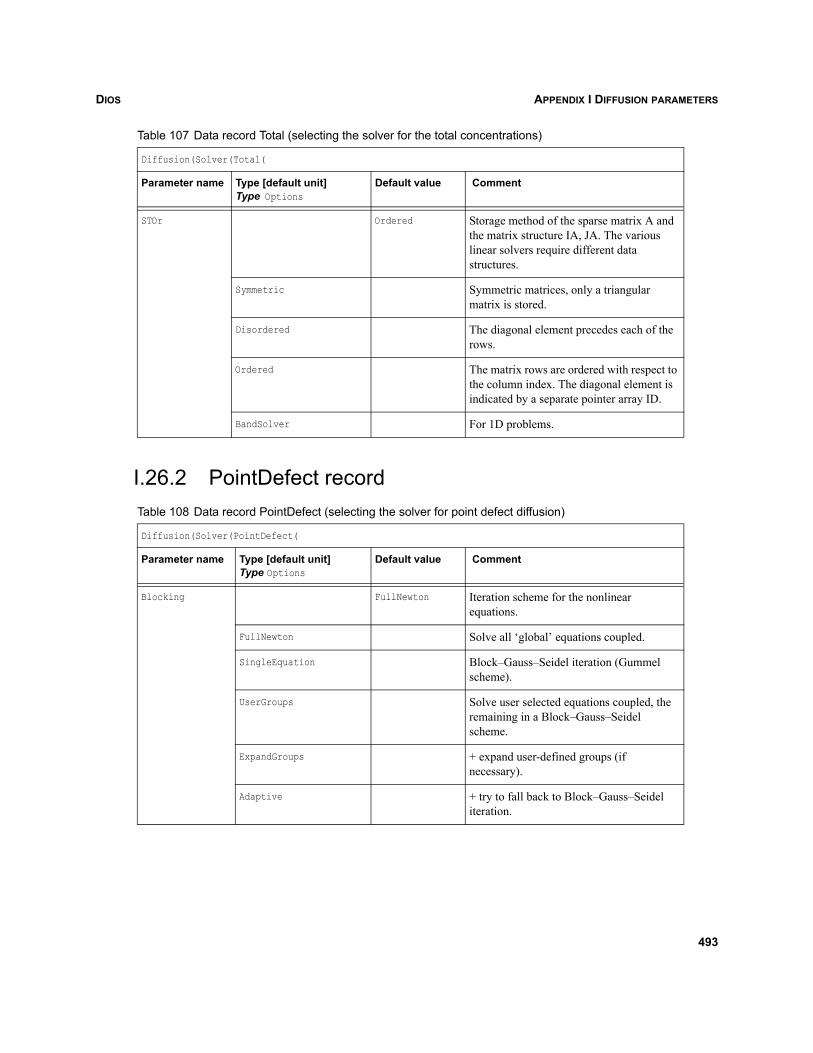
DIOS APPENDIX I DIFFUSION PARAMETERS
I.26.2 PointDefect record
STOr Ordered Storage method of the sparse matrix A and the matrix structure IA, JA. The various linear solvers require different data structures.
Symmetric Symmetric matrices, only a triangular matrix is stored.
Disordered The diagonal element precedes each of the rows.
Ordered The matrix rows are ordered with respect to the column index. The diagonal element is indicated by a separate pointer array ID.
BandSolver For 1D problems.
Table 108 Data record PointDefect (selecting the solver for point defect diffusion)
Diffusion(Solver(PointDefect(
Parameter name Type [default unit]Type Options
Default value Comment
Blocking FullNewton Iteration scheme for the nonlinear equations.
FullNewton Solve all ‘global’ equations coupled.
SingleEquation Block–Gauss–Seidel iteration (Gummel scheme).
UserGroups Solve user selected equations coupled, the remaining in a Block–Gauss–Seidel scheme.
ExpandGroups + expand user-defined groups (if necessary).
Adaptive + try to fall back to Block–Gauss–Seidel iteration.
Table 107 Data record Total (selecting the solver for the total concentrations)
Diffusion(Solver(Total(
Parameter name Type [default unit]Type Options
Default value Comment
493
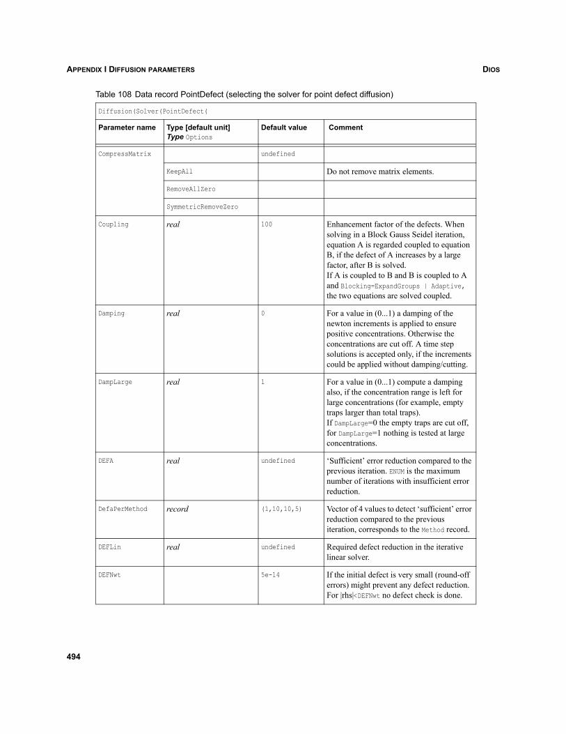
DIOSAPPENDIX I DIFFUSION PARAMETERS
CompressMatrix undefined
KeepAll Do not remove matrix elements.
RemoveAllZero
SymmetricRemoveZero
Coupling real 100 Enhancement factor of the defects. When solving in a Block Gauss Seidel iteration, equation A is regarded coupled to equation B, if the defect of A increases by a large factor, after B is solved.If A is coupled to B and B is coupled to A and Blocking=ExpandGroups | Adaptive, the two equations are solved coupled.
Damping real 0 For a value in (0...1) a damping of the newton increments is applied to ensure positive concentrations. Otherwise the concentrations are cut off. A time step solutions is accepted only, if the increments could be applied without damping/cutting.
DampLarge real 1 For a value in (0...1) compute a damping also, if the concentration range is left for large concentrations (for example, empty traps larger than total traps).If DampLarge=0 the empty traps are cut off, for DampLarge=1 nothing is tested at large concentrations.
DEFA real undefined ‘Sufficient’ error reduction compared to the previous iteration. ENUM is the maximum number of iterations with insufficient error reduction.
DefaPerMethod record (1,10,10,5) Vector of 4 values to detect ‘sufficient’ error reduction compared to the previous iteration, corresponds to the Method record.
DEFLin real undefined Required defect reduction in the iterative linear solver.
DEFNwt 5e-14 If the initial defect is very small (round-off errors) might prevent any defect reduction. For |rhs|<DEFNwt no defect check is done.
Table 108 Data record PointDefect (selecting the solver for point defect diffusion)
Diffusion(Solver(PointDefect(
Parameter name Type [default unit]Type Options
Default value Comment
494
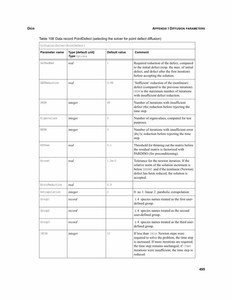
DIOS APPENDIX I DIFFUSION PARAMETERS
DefRedNwt real 1 Required reduction of the defect, compared to the initial defect (resp. the max. of initial defect, and defect after the first iteration) before accepting the solution.
DEFReduction real 0.98 ‘Sufficient’ reduction of the (nonlinear) defect (compared to the previous iteration). DNUM is the maximum number of iterations with insufficient defect reduction.
DNUM integer 40 Number of iterations with insufficient defect |rhs| reduction before rejecting the time step.
Eigenvalues integer 0 Number of eigenvalues, computed for test purposes.
ENUM integer 3 Number of iterations with insufficient error |dx|/|x| reduction before rejecting the time step.
EPSUwe real 0.1 Threshold for thinning out the matrix before the residual matrix is factorized with PARDISO (for preconditioning).
Errnwt real 1.5e-3 Tolerance for the newton iteration. If the relative norm of the solution increment is below ERRNWT and if the nonlinear (Newton) defect has been reduced, the solution is accepted.
ErrorReduction real 0.9
Extrapolation integer 2 0: no 1: linear 2: parabolic extrapolation.
Group1 record species names treated as the first user-defined group.
Group2 record species names treated as the second user-defined group.
Group3 record species names treated as the third user-defined group.
INCdt integer 12 If less than INCdt Newton steps were required to solve the problem, the time step is increased. If more iterations are required, the time step remains unchanged, if ITNWT iterations were insufficient, the time step is reduced.
Table 108 Data record PointDefect (selecting the solver for point defect diffusion)
Diffusion(Solver(PointDefect(
Parameter name Type [default unit]Type Options
Default value Comment
4≤
4≤
4≤
495
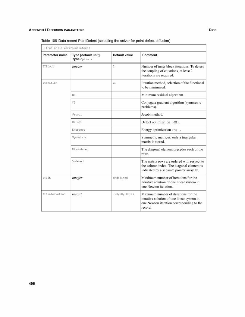
DIOSAPPENDIX I DIFFUSION PARAMETERS
ITBLock integer 2 Number of inner block iterations. To detect the coupling of equations, at least 2 iterations are required.
Iteration CG Iteration method, selection of the functional to be minimized.
MR Minimum residual algorithm.
CG Conjugate gradient algorithm (symmetric problems).
Jacobi Jacobi method.
Defopt Defect optimization (=MR).
Energopt Energy optimization (=CG).
Symmetric Symmetric matrices, only a triangular matrix is stored.
Disordered The diagonal element precedes each of the rows.
Ordered The matrix rows are ordered with respect to the column index. The diagonal element is indicated by a separate pointer array ID.
ITLin integer undefined Maximum number of iterations for the iterative solution of one linear system in one Newton iteration.
ItLinPerMethod record (20,50,100,4) Maximum number of iterations for the iterative solution of one linear system in one Newton iteration corresponding to the record.
Table 108 Data record PointDefect (selecting the solver for point defect diffusion)
Diffusion(Solver(PointDefect(
Parameter name Type [default unit]Type Options
Default value Comment
496
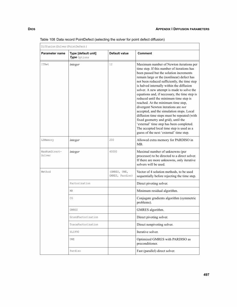
DIOS APPENDIX I DIFFUSION PARAMETERS
ITNwt integer 12 Maximum number of Newton iterations per time step. If this number of iterations has been passed but the solution increments remain large or the (nonlinear) defect has not been reduced sufficiently, the time step is halved internally within the diffusion solver. A new attempt is made to solve the equations and, if necessary, the time step is reduced until the minimum time step is reached. At the minimum time step, divergent Newton iterations are not accepted, and the simulation stops. Local diffusion time steps must be repeated (with fixed geometry and grid), until the ‘external’ time step has been completed. The accepted local time step is used as a guess of the next ‘external’ time step.
LSMemory integer 200 Allowed extra memory for PARDISO in MB.
MaxNumDirect-Solver
integer 40000 Maximal number of unknowns (per processor) to be directed to a direct solver. If there are more unknowns, only iterative solvers will be used.
Method (GMRES, UWE, GMRES, Pardiso)
Vector of 4 solution methods, to be used sequentially before rejecting the time step.
Factorization Direct pivoting solver.
MR Minimum residual algorithm.
CG Conjugate gradients algorithm (symmetric problems).
GMRES GMRES algorithm.
GrundFactorization Direct pivoting solver.
ToscaFactorization Direct nonpivoting solver.
SLIP90 Iterative solver.
UWE Optimized GMRES with PARDISO as preconditioner.
Pardiso Fast (parallel) direct solver.
Table 108 Data record PointDefect (selecting the solver for point defect diffusion)
Diffusion(Solver(PointDefect(
Parameter name Type [default unit]Type Options
Default value Comment
497
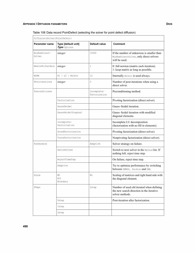
DIOSAPPENDIX I DIFFUSION PARAMETERS
MinNumDirect-Solver
integer 15000 If the number of unknowns is smaller than MinNumDirectSolver, only direct solvers will be used.
NewtonRichardson integer 1 0: full newton (matrix each iteration).1: keep matrix as long as possible.
NORM H1 | L2 | Relerr L2 Internally Relerr is used always.
POstiterations integer 0 Number of post-iterations when using a direct solver.
Preconditioner Incomplete-Factorization
Preconditioning method.
Factorization Pivoting factorization (direct solver).
GaussSeidel Gauss–Seidel iteration.
GaussSeidelDiagonal Gauss–Seidel iteration with modified diagonal elements.
Incomplete-Factorization
Incomplete LU decomposition (factorization with no fill in elements).
GrundFactorization Pivoting factorization (direct solver).
ToscaFactorization Nonpivoting factorization (direct solver).
Preference Adaptive Solver strategy on failure.
SwitchSolver Switch to next solver in the Method list. If nothing left, reject time step.
RejectTimeStep On failure, reject time step.
Adaptive Try to optimize performance by switching between GMRES, Pardiso and UWE.
Scale NOAllBoundary
No Scaling of matrices and right hand side with the diagonal element.
STeps 2step Number of used old iterated when defining the new search direction in the iterative solver methods.
0step Post-iteration after factorization.
1step
2step
Table 108 Data record PointDefect (selecting the solver for point defect diffusion)
Diffusion(Solver(PointDefect(
Parameter name Type [default unit]Type Options
Default value Comment
498

DIOS APPENDIX I DIFFUSION PARAMETERS
STOr Ordered Storage method of the sparse matrix A and the matrix structure IA, JA. The various linear solvers require different data structures: Ordered, Symmetric, Disordered, BandSolver.
Time-Discretization
EulerGierTrapez TrBDF2BDF1 BDF2
Euler Time discretization method.
TruncationError boolean off Compute local truncation error (not tested).
Table 108 Data record PointDefect (selecting the solver for point defect diffusion)
Diffusion(Solver(PointDefect(
Parameter name Type [default unit]Type Options
Default value Comment
499

DIOSAPPENDIX I DIFFUSION PARAMETERS
500
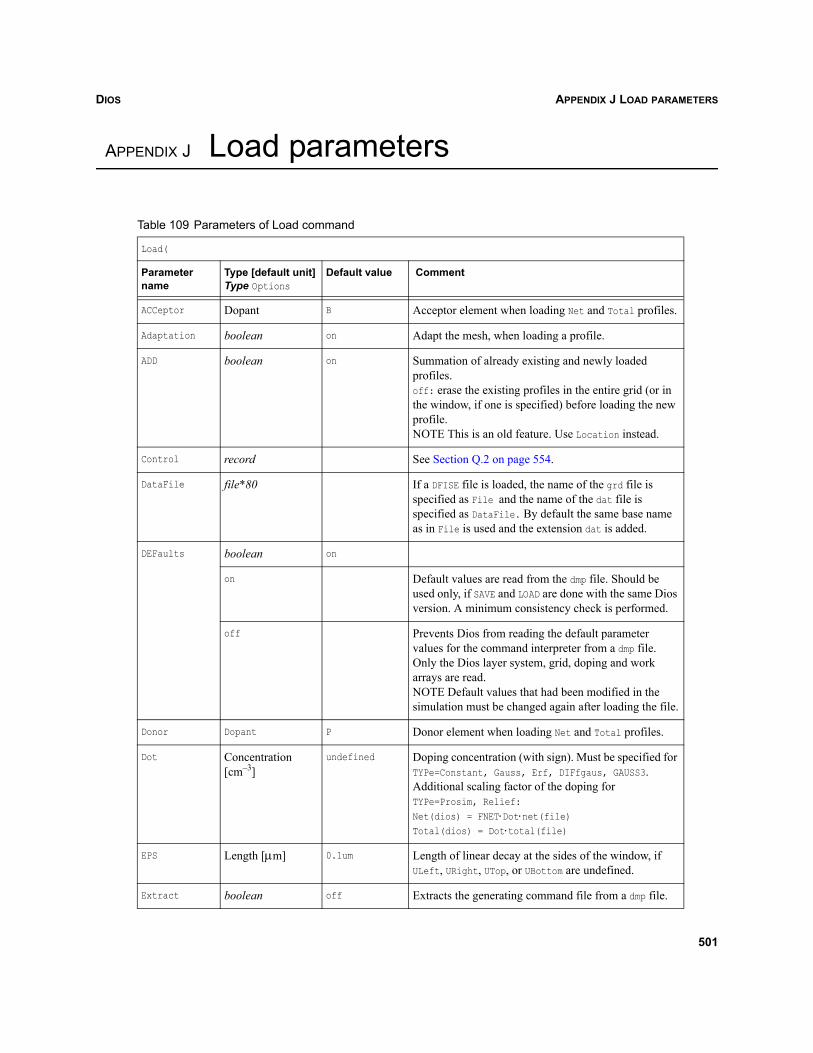
DIOS APPENDIX J LOAD PARAMETERS
Dios
APPENDIX J Load parameters
Table 109 Parameters of Load command
Load(
Parameter name
Type [default unit]Type Options
Default value Comment
ACCeptor Dopant B Acceptor element when loading Net and Total profiles.
Adaptation boolean on Adapt the mesh, when loading a profile.
ADD boolean on Summation of already existing and newly loaded profiles.off: erase the existing profiles in the entire grid (or in the window, if one is specified) before loading the new profile.NOTE This is an old feature. Use Location instead.
Control record See Section Q.2 on page 554.
DataFile file*80 If a DFISE file is loaded, the name of the grd file is specified as File and the name of the dat file is specified as DataFile. By default the same base name as in File is used and the extension dat is added.
DEFaults boolean on
on Default values are read from the dmp file. Should be used only, if SAVE and LOAD are done with the same Dios version. A minimum consistency check is performed.
off Prevents Dios from reading the default parameter values for the command interpreter from a dmp file. Only the Dios layer system, grid, doping and work arrays are read. NOTE Default values that had been modified in the simulation must be changed again after loading the file.
Donor Dopant P Donor element when loading Net and Total profiles.
Dot Concentration [cm–3]
undefined Doping concentration (with sign). Must be specified for TYPe=Constant, Gauss, Erf, DIFfgaus, GAUSS3.Additional scaling factor of the doping for TYPe=Prosim, Relief:Net(dios) = FNET⋅Dot⋅net(file)Total(dios) = Dot⋅total(file)
EPS Length [μm] 0.1um Length of linear decay at the sides of the window, if ULeft, URight, UTop, or UBottom are undefined.
Extract boolean off Extracts the generating command file from a dmp file.
501
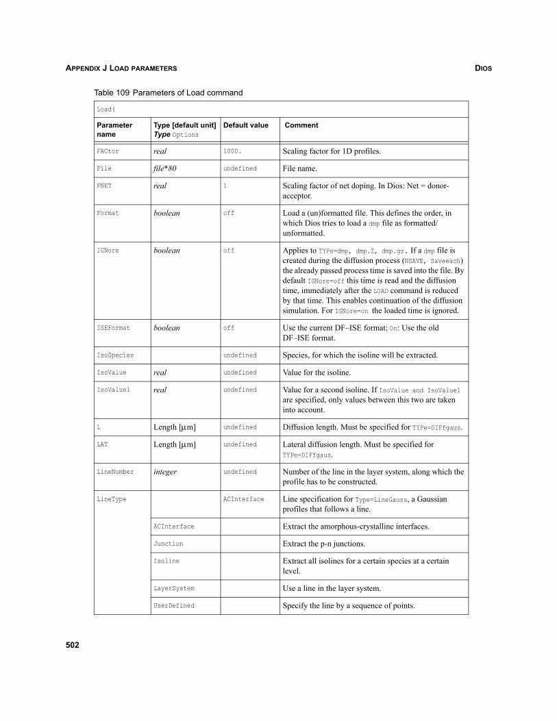
DIOSAPPENDIX J LOAD PARAMETERS
FACtor real 1000. Scaling factor for 1D profiles.
File file*80 undefined File name.
FNET real 1 Scaling factor of net doping. In Dios: Net = donor-acceptor.
Format boolean off Load a (un)formatted file. This defines the order, in which Dios tries to load a dmp file as formatted/unformatted.
IGNore boolean off Applies to TYPe=dmp, dmp.Z, dmp.gz. If a dmp file is created during the diffusion process (NSAVE, Saveeach) the already passed process time is saved into the file. By default IGNore=off this time is read and the diffusion time, immediately after the LOAD command is reduced by that time. This enables continuation of the diffusion simulation. For IGNore=on the loaded time is ignored.
ISEFormat boolean off Use the current DF–ISE format; On: Use the old DF–ISE format.
IsoSpecies undefined Species, for which the isoline will be extracted.
IsoValue real undefined Value for the isoline.
IsoValue1 real undefined Value for a second isoline. If IsoValue and IsoValue1 are specified, only values between this two are taken into account.
L Length [μm] undefined Diffusion length. Must be specified for TYPe=DIFfgaus.
LAT Length [μm] undefined Lateral diffusion length. Must be specified for TYPe=DIFfgaus.
LineNumber integer undefined Number of the line in the layer system, along which the profile has to be constructed.
LineType ACInterface Line specification for Type=LineGauss, a Gaussian profiles that follows a line.
ACInterface Extract the amorphous-crystalline interfaces.
Junction Extract the p-n junctions.
Isoline Extract all isolines for a certain species at a certain level.
LayerSystem Use a line in the layer system.
UserDefined Specify the line by a sequence of points.
Table 109 Parameters of Load command
Load(
Parameter name
Type [default unit]Type Options
Default value Comment
502
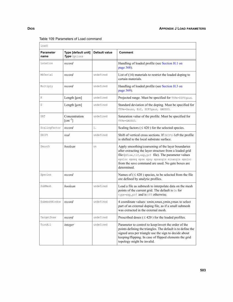
DIOS APPENDIX J LOAD PARAMETERS
Location record Handling of loaded profile (see Section H.1 on page 368).
MATerial record undefined List of (14) materials to restrict the loaded doping to certain materials.
Multiply record undefined Handling of loaded profile (see Section H.3 on page 369).
R Length [μm] undefined Projected range. Must be specified for TYPe=DIFfgaus.
S Length [μm] undefined Standard deviation of the doping. Must be specified for TYPe=Gauss, Erf, DIFfgaus, GAUSS3.
SAT Concentration [cm–3]
undefined Saturation value of the profile. Must be specified for TYPe=GAUSS3.
ScalingFactor record 1. Scaling factors ( ) for the selected species.
SHIFt real undefined Shift of vertical cross sections. If SHIFt>1e9 the profile is shifted to the local substrate surface.
Smooth boolean on Apply smoothing/coarsening of the layer boundaries after extracting the layer structure from a loaded grid file (dfise,tif,exp,prf file). The parameter values epsloc epseq epsx epsy epsangle minangle epsloc from the save command are used. No gate boxes are determined.
Species record Names of ( ) species, to be selected from the file ore defined by analytic profiles.
SubMesh boolean undefined Load a file as submesh to interpolate data on the mesh points of the current grid. The default is On for type=exp,prf and is Off otherwise.
SubmeshWindow record undefined 4 coordinate values: xmin,xmax,ymin,ymax to select part of an external doping file, as if a small submesh was extracted in the external mesh.
TargetDose record undefined Prescribed doses ( ) for the loaded profiles.
TurnAll integer undefined Parameter to control to keep/invert the order of the points defining the triangles. The default is to define the signed area per triangle use the sign to decide about keeping/flipping. In case of flipped elements the grid topology might be invalid.
Table 109 Parameters of Load command
Load(
Parameter name
Type [default unit]Type Options
Default value Comment
420≤
420≤
420≤
503
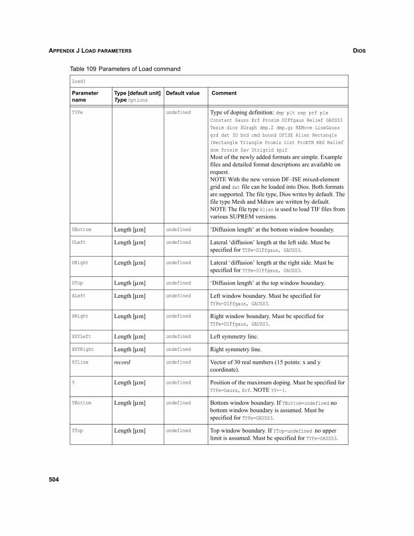
DIOSAPPENDIX J LOAD PARAMETERS
TYPe undefined Type of doping definition: dmp plt exp prf plx Constant Gauss Erf Prosim DIFfgaus Relief GAUSS3 Tesim dios XGraph dmp.Z dmp.gz REMove LineGauss grd dat 3D bnd cmd bound DFISE Alien Rectangle IRectangle Triangle Promis List ProETH RES Relief dom Prosim Sav Utrigrid kpifMost of the newly added formats are simple. Example files and detailed format descriptions are available on request.NOTE With the new version DF–ISE mixed-element grid and dat file can be loaded into Dios. Both formats are supported. The file type, Dios writes by default. The file type Mesh and Mdraw are written by default.NOTE The file type Alien is used to load TIF files from various SUPREM versions.
UBottom Length [μm] undefined ‘Diffusion length’ at the bottom window boundary.
ULeft Length [μm] undefined Lateral ‘diffusion’ length at the left side. Must be specified for TYPe=DIFfgaus, GAUSS3.
URight Length [μm] undefined Lateral ‘diffusion’ length at the right side. Must be specified for TYPe=DIFfgaus, GAUSS3.
UTop Length [μm] undefined ‘Diffusion length’ at the top window boundary.
XLeft Length [μm] undefined Left window boundary. Must be specified for TYPe=DIFfgaus, GAUSS3.
XRight Length [μm] undefined Right window boundary. Must be specified for TYPe=DIFfgaus, GAUSS3.
XSYLeft Length [μm] undefined Left symmetry line.
XSYRight Length [μm] undefined Right symmetry line.
XYLine record undefined Vector of 30 real numbers (15 points: x and y coordinate).
Y Length [μm] undefined Position of the maximum doping. Must be specified for TYPe=Gauss, Erf. NOTE YY=-1.
YBottom Length [μm] undefined Bottom window boundary. If YBottom=undefined no bottom window boundary is assumed. Must be specified for TYPe=GAUSS3.
YTop Length [μm] undefined Top window boundary. If YTop=undefined no upper limit is assumed. Must be specified for TYPe=GAUSS3.
Table 109 Parameters of Load command
Load(
Parameter name
Type [default unit]Type Options
Default value Comment
504
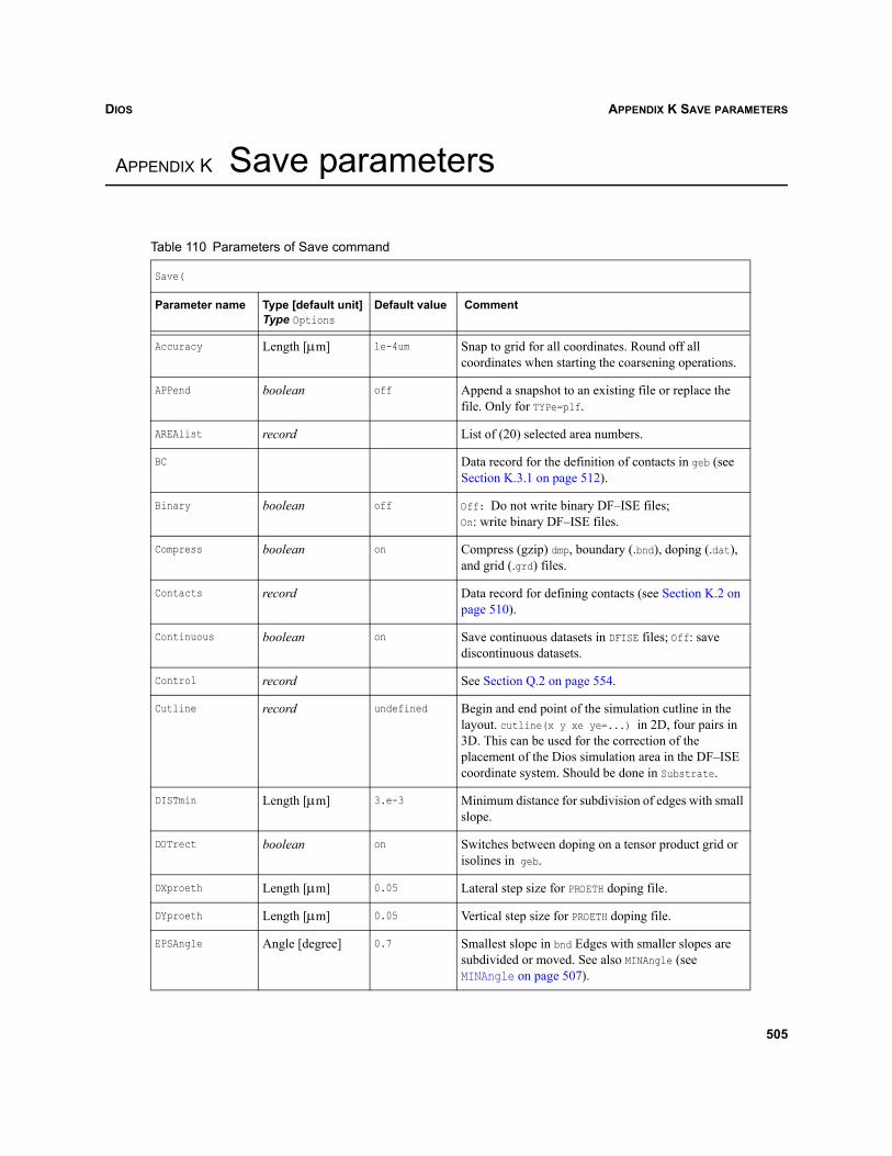
DIOS APPENDIX K SAVE PARAMETERS
Dios
APPENDIX K Save parameters
Table 110 Parameters of Save command
Save(
Parameter name Type [default unit]Type Options
Default value Comment
Accuracy Length [μm] 1e-4um Snap to grid for all coordinates. Round off all coordinates when starting the coarsening operations.
APPend boolean off Append a snapshot to an existing file or replace the file. Only for TYPe=plf.
AREAlist record List of (20) selected area numbers.
BC Data record for the definition of contacts in geb (see Section K.3.1 on page 512).
Binary boolean off Off: Do not write binary DF–ISE files; On: write binary DF–ISE files.
Compress boolean on Compress (gzip) dmp, boundary (.bnd), doping (.dat), and grid (.grd) files.
Contacts record Data record for defining contacts (see Section K.2 on page 510).
Continuous boolean on Save continuous datasets in DFISE files; Off: save discontinuous datasets.
Control record See Section Q.2 on page 554.
Cutline record undefined Begin and end point of the simulation cutline in the layout. cutline(x y xe ye=...) in 2D, four pairs in 3D. This can be used for the correction of the placement of the Dios simulation area in the DF–ISE coordinate system. Should be done in Substrate.
DISTmin Length [μm] 3.e-3 Minimum distance for subdivision of edges with small slope.
DOTrect boolean on Switches between doping on a tensor product grid or isolines in geb.
DXproeth Length [μm] 0.05 Lateral step size for PROETH doping file.
DYproeth Length [μm] 0.05 Vertical step size for PROETH doping file.
EPSAngle Angle [degree] 0.7 Smallest slope in bnd Edges with smaller slopes are subdivided or moved. See also MINAngle (see MINAngle on page 507).
505
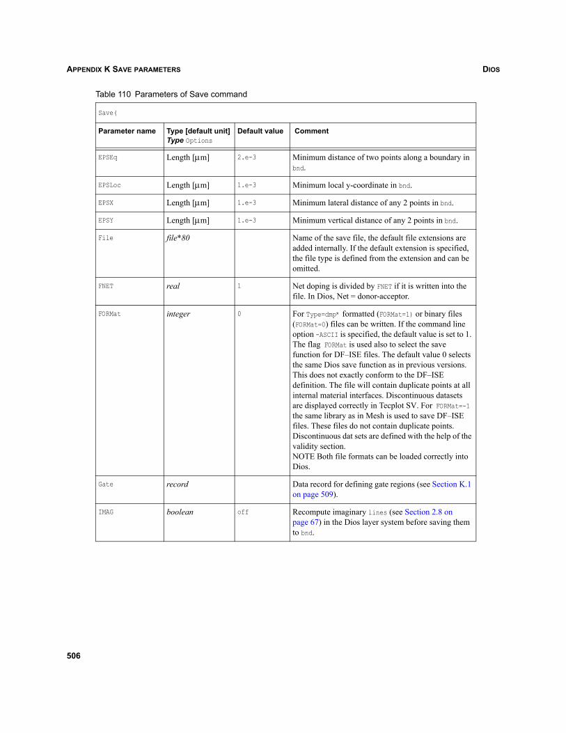
DIOSAPPENDIX K SAVE PARAMETERS
EPSEq Length [μm] 2.e-3 Minimum distance of two points along a boundary in bnd.
EPSLoc Length [μm] 1.e-3 Minimum local y-coordinate in bnd.
EPSX Length [μm] 1.e-3 Minimum lateral distance of any 2 points in bnd.
EPSY Length [μm] 1.e-3 Minimum vertical distance of any 2 points in bnd.
File file*80 Name of the save file, the default file extensions are added internally. If the default extension is specified, the file type is defined from the extension and can be omitted.
FNET real 1 Net doping is divided by FNET if it is written into the file. In Dios, Net = donor-acceptor.
FORMat integer 0 For Type=dmp* formatted (FORMat=1) or binary files (FORMat=0) files can be written. If the command line option -ASCII is specified, the default value is set to 1. The flag FORMat is used also to select the save function for DF–ISE files. The default value 0 selects the same Dios save function as in previous versions. This does not exactly conform to the DF–ISE definition. The file will contain duplicate points at all internal material interfaces. Discontinuous datasets are displayed correctly in Tecplot SV. For FORMat=-1 the same library as in Mesh is used to save DF–ISE files. These files do not contain duplicate points. Discontinuous dat sets are defined with the help of the validity section. NOTE Both file formats can be loaded correctly into Dios.
Gate record Data record for defining gate regions (see Section K.1 on page 509).
IMAG boolean off Recompute imaginary lines (see Section 2.8 on page 67) in the Dios layer system before saving them to bnd.
Table 110 Parameters of Save command
Save(
Parameter name Type [default unit]Type Options
Default value Comment
506
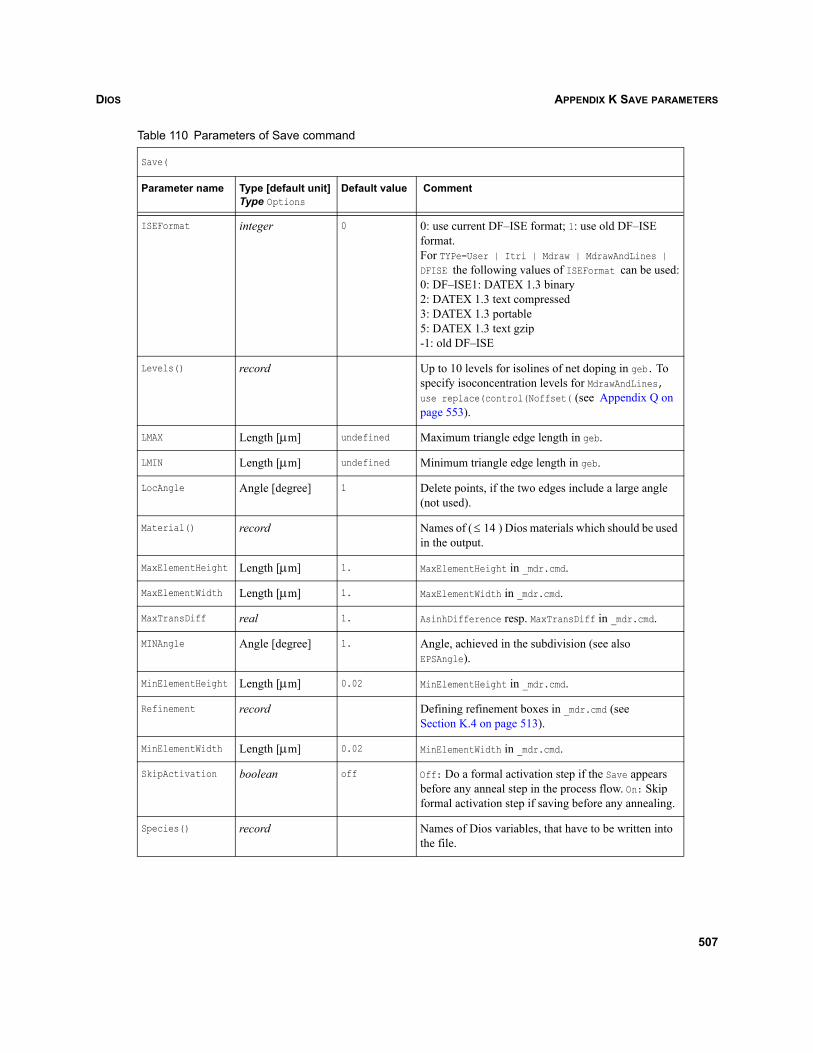
DIOS APPENDIX K SAVE PARAMETERS
ISEFormat integer 0 0: use current DF–ISE format; 1: use old DF–ISE format.For TYPe=User | Itri | Mdraw | MdrawAndLines | DFISE the following values of ISEFormat can be used:0: DF–ISE1: DATEX 1.3 binary2: DATEX 1.3 text compressed3: DATEX 1.3 portable5: DATEX 1.3 text gzip-1: old DF–ISE
Levels() record Up to 10 levels for isolines of net doping in geb. To specify isoconcentration levels for MdrawAndLines, use replace(control(Noffset( (see Appendix Q on page 553).
LMAX Length [μm] undefined Maximum triangle edge length in geb.
LMIN Length [μm] undefined Minimum triangle edge length in geb.
LocAngle Angle [degree] 1 Delete points, if the two edges include a large angle (not used).
Material() record Names of ( ) Dios materials which should be used in the output.
MaxElementHeight Length [μm] 1. MaxElementHeight in _mdr.cmd.
MaxElementWidth Length [μm] 1. MaxElementWidth in _mdr.cmd.
MaxTransDiff real 1. AsinhDifference resp. MaxTransDiff in _mdr.cmd.
MINAngle Angle [degree] 1. Angle, achieved in the subdivision (see also EPSAngle).
MinElementHeight Length [μm] 0.02 MinElementHeight in _mdr.cmd.
Refinement record Defining refinement boxes in _mdr.cmd (see Section K.4 on page 513).
MinElementWidth Length [μm] 0.02 MinElementWidth in _mdr.cmd.
SkipActivation boolean off Off: Do a formal activation step if the Save appears before any anneal step in the process flow. On: Skip formal activation step if saving before any annealing.
Species() record Names of Dios variables, that have to be written into the file.
Table 110 Parameters of Save command
Save(
Parameter name Type [default unit]Type Options
Default value Comment
14≤
507
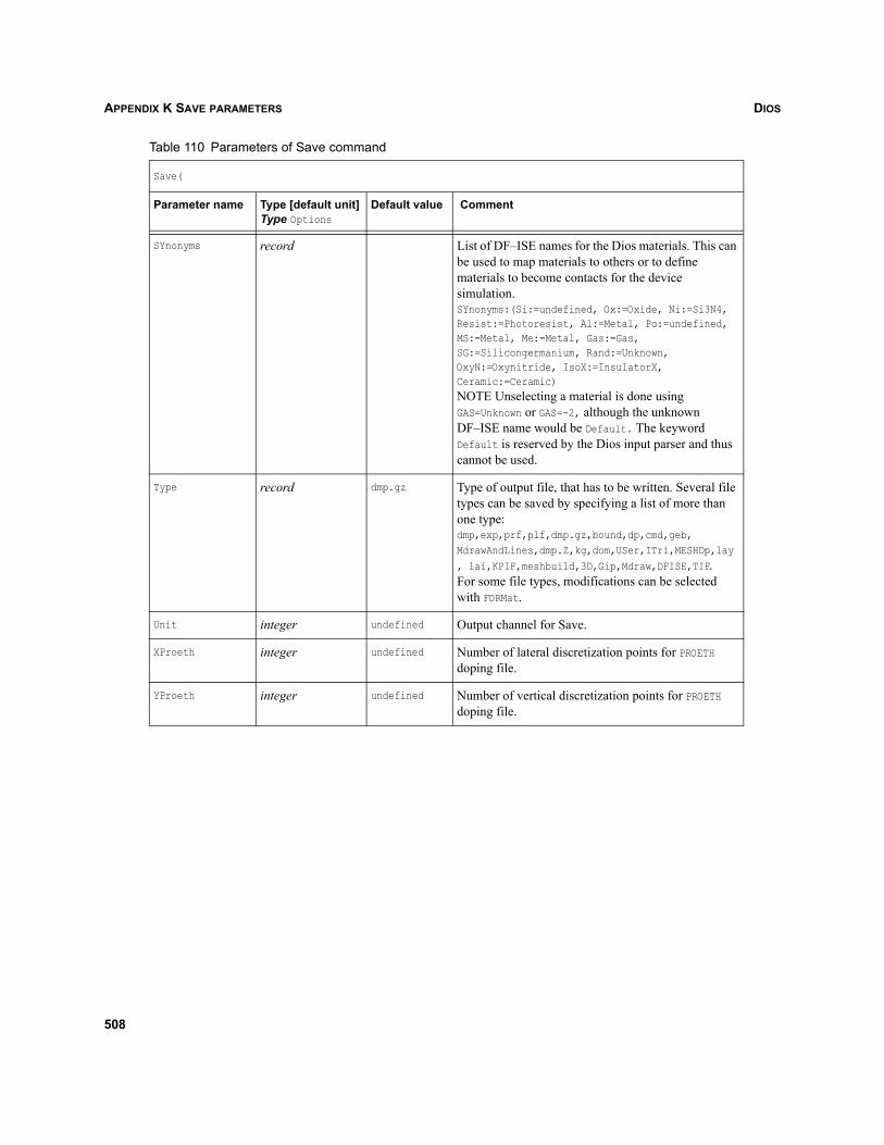
DIOSAPPENDIX K SAVE PARAMETERS
SYnonyms record List of DF–ISE names for the Dios materials. This can be used to map materials to others or to define materials to become contacts for the device simulation.SYnonyms:(Si:=undefined, Ox:=Oxide, Ni:=Si3N4, Resist:=Photoresist, Al:=Metal, Po:=undefined, MS:=Metal, Me:=Metal, Gas:=Gas, SG:=Silicongermanium, Rand:=Unknown, OxyN:=Oxynitride, IsoX:=InsulatorX, Ceramic:=Ceramic)NOTE Unselecting a material is done using GAS=Unknown or GAS=-2, although the unknown DF–ISE name would be Default. The keyword Default is reserved by the Dios input parser and thus cannot be used.
Type record dmp.gz Type of output file, that has to be written. Several file types can be saved by specifying a list of more than one type:dmp,exp,prf,plf,dmp.gz,bound,dp,cmd,geb,MdrawAndLines,dmp.Z,kg,dom,USer,ITri,MESHDp,lay, lai,KPIF,meshbuild,3D,Gip,Mdraw,DFISE,TIF.For some file types, modifications can be selected with FORMat.
Unit integer undefined Output channel for Save.
XProeth integer undefined Number of lateral discretization points for PROETH doping file.
YProeth integer undefined Number of vertical discretization points for PROETH doping file.
Table 110 Parameters of Save command
Save(
Parameter name Type [default unit]Type Options
Default value Comment
508
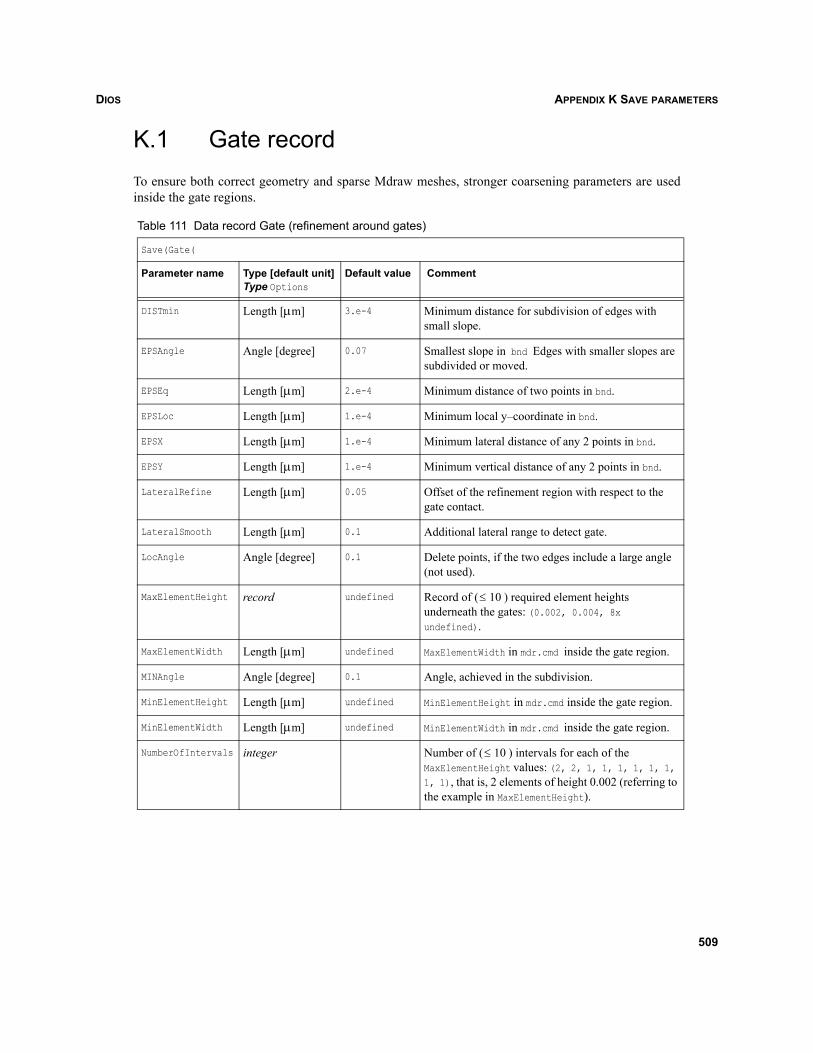
DIOS APPENDIX K SAVE PARAMETERS
K.1 Gate recordTo ensure both correct geometry and sparse Mdraw meshes, stronger coarsening parameters are usedinside the gate regions.
Table 111 Data record Gate (refinement around gates)
Save(Gate(
Parameter name Type [default unit]Type Options
Default value Comment
DISTmin Length [μm] 3.e-4 Minimum distance for subdivision of edges with small slope.
EPSAngle Angle [degree] 0.07 Smallest slope in bnd Edges with smaller slopes are subdivided or moved.
EPSEq Length [μm] 2.e-4 Minimum distance of two points in bnd.
EPSLoc Length [μm] 1.e-4 Minimum local y–coordinate in bnd.
EPSX Length [μm] 1.e-4 Minimum lateral distance of any 2 points in bnd.
EPSY Length [μm] 1.e-4 Minimum vertical distance of any 2 points in bnd.
LateralRefine Length [μm] 0.05 Offset of the refinement region with respect to the gate contact.
LateralSmooth Length [μm] 0.1 Additional lateral range to detect gate.
LocAngle Angle [degree] 0.1 Delete points, if the two edges include a large angle (not used).
MaxElementHeight record undefined Record of ( ) required element heights underneath the gates: (0.002, 0.004, 8x undefined).
MaxElementWidth Length [μm] undefined MaxElementWidth in mdr.cmd inside the gate region.
MINAngle Angle [degree] 0.1 Angle, achieved in the subdivision.
MinElementHeight Length [μm] undefined MinElementHeight in mdr.cmd inside the gate region.
MinElementWidth Length [μm] undefined MinElementWidth in mdr.cmd inside the gate region.
NumberOfIntervals integer Number of ( ) intervals for each of the MaxElementHeight values: (2, 2, 1, 1, 1, 1, 1, 1, 1, 1), that is, 2 elements of height 0.002 (referring to the example in MaxElementHeight).
10≤
10≤
509
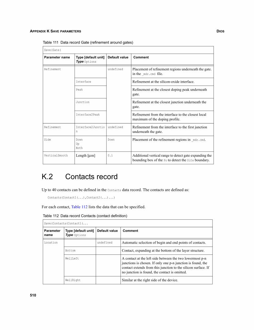
DIOSAPPENDIX K SAVE PARAMETERS
K.2 Contacts recordUp to 40 contacts can be defined in the Contacts data record. The contacts are defined as:
Contacts(Contact1(...),Contact2(...)...)
For each contact, Table 112 lists the data that can be specified.
Refinement undefined Placement of refinement regions underneath the gate. in the _mdr.cmd file.
Interface Refinement at the silicon-oxide interface.
Peak Refinement at the closest doping peak underneath gate.
Junction Refinement at the closest junction underneath the gate.
Interface2Peak Refinement from the interface to the closest local maximum of the doping profile.
Refinement Interface2Junction
undefined Refinement from the interface to the first junction underneath the gate.
Side DownUpBoth
Down Placement of the refinement regions in _mdr.cmd.
VerticalSmooth Length [μm] 0.1 Additional vertical range to detect gate expanding the bounding box of the Po to detect the SiOx boundary.
Table 112 Data record Contacts (contact definition)
Save(Contacts(Contact1(...
Parameter name
Type [default unit]Type Options
Default value Comment
Location undefined Automatic selection of begin and end points of contacts.
Bottom Contact, expanding at the bottom of the layer structure.
WellLeft A contact at the left side between the two lowermost p-n junctions is chosen. If only one p-n junction is found, the contact extends from this junction to the silicon surface. If no junction is found, the contact is omitted.
WellRight Similar at the right side of the device.
Table 111 Data record Gate (refinement around gates)
Save(Gate(
Parameter name Type [default unit]Type Options
Default value Comment
510
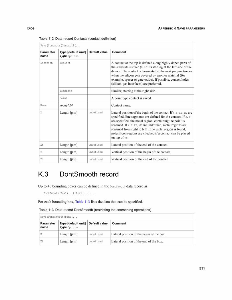
DIOS APPENDIX K SAVE PARAMETERS
K.3 DontSmooth recordUp to 40 bounding boxes can be defined in the DontSmooth data record as:
DontSmooth(Box1(...),Box2(...)...)
For each bounding box, Table 113 lists the data that can be specified.
Location TopLeft A contact at the top is defined along highly doped parts of the substrate surface (> 1e19) starting at the left side of the device. The contact is terminated at the next p-n junction or when the silicon gets covered by another material (for example, spacer or gate oxide). If possible, contact holes (silicon-gas interfaces) are preferred.
TopRight Similar, starting at the right side.
Point A point type contact is saved.
Name string*24 Contact name.
X Length [μm] undefined Lateral position of the begin of the contact. If X,Y,XE,YE are specified, line segments are defined for the contact. If X,Y are specified, the metal region, containing the point is renamed. If X,Y,XE,YE are undefined, metal regions are renamed from right to left. If no metal region is found, polysilicon regions are checked if a contact can be placed on top of Po.
XE Length [μm] undefined Lateral position of the end of the contact.
Y Length [μm] undefined Vertical position of the begin of the contact.
YE Length [μm] undefined Vertical position of the end of the contact.
Table 113 Data record DontSmooth (restricting the coarsening operations)
Save(DontSmooth(Box1(...
Parameter name
Type [default unit]Type Options
Default value Comment
X Length [μm] undefined Lateral position of the begin of the box.
XE Length [μm] undefined Lateral position of the end of the box.
Table 112 Data record Contacts (contact definition)
Save(Contacts(Contact1(...
Parameter name
Type [default unit]Type Options
Default value Comment
511
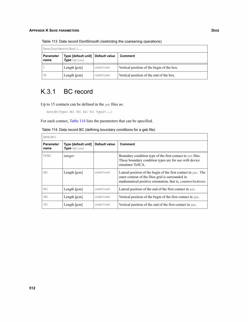
DIOSAPPENDIX K SAVE PARAMETERS
K.3.1 BC record
Up to 15 contacts can be defined in the geb files as:
Save(BC(Type1 Xb1 Yb1 Xe1 Ye1 Type2=...)
For each contact, Table 114 lists the parameters that can be specified.
Y Length [μm] undefined Vertical position of the begin of the box.
YE Length [μm] undefined Vertical position of the end of the box.
Table 114 Data record BC (defining boundary conditions for a geb file)
SAVE(BC(
Parameter name
Type [default unit]Type Options
Default value Comment
TYPE1 integer Boundary condition type of the first contact in geb files. These boundary condition types are for use with device simulator TeSCA.
XB1 Length [μm] undefined Lateral position of the begin of the first contact in geb. The outer contour of the Dios grid is surrounded in mathematical positive orientation, that is, counterclockwise.
XE1 Length [μm] undefined Lateral position of the end of the first contact in geb.
YB1 Length [μm] undefined Vertical position of the begin of the first contact in geb.
YE1 Length [μm] undefined Vertical position of the end of the first contact in geb.
Table 113 Data record DontSmooth (restricting the coarsening operations)
Save(DontSmooth(Box1(...
Parameter name
Type [default unit]Type Options
Default value Comment
512
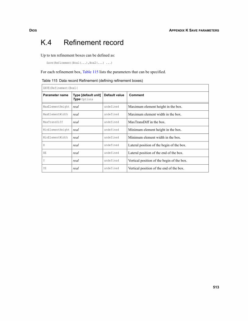
DIOS APPENDIX K SAVE PARAMETERS
K.4 Refinement recordUp to ten refinement boxes can be defined as:
Save(Refinement(Box1(...),Box2(...) ...)
For each refinement box, Table 115 lists the parameters that can be specified.
Table 115 Data record Refinement (defining refinement boxes)
SAVE(Refinement(Box1(
Parameter name Type [default unit]Type Options
Default value Comment
MaxElementHeight real undefined Maximum element height in the box.
MaxElementWidth real undefined Maximum element width in the box.
MaxTransDiff real undefined MaxTransDiff in the box.
MinElementHeight real undefined Minimum element height in the box.
MinElementWidth real undefined Minimum element width in the box.
X real undefined Lateral position of the begin of the box.
XE real undefined Lateral position of the end of the box.
Y real undefined Vertical position of the begin of the box.
YE real undefined Vertical position of the end of the box.
513

DIOSAPPENDIX K SAVE PARAMETERS
514
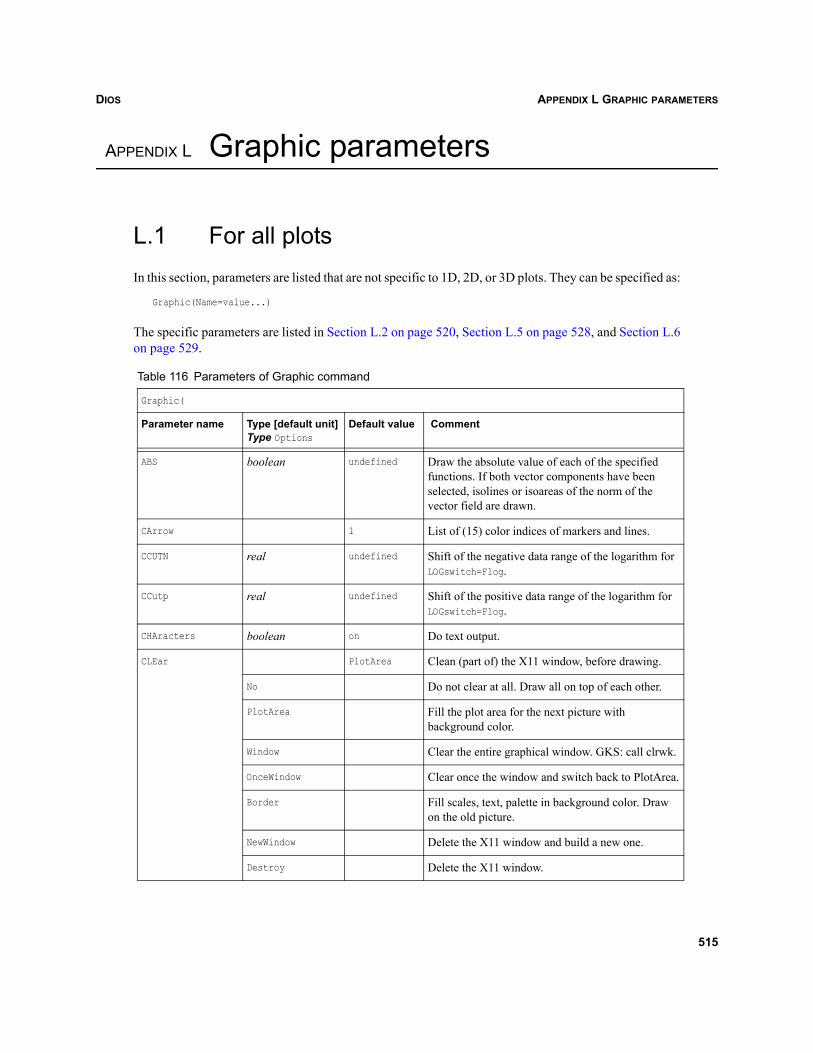
DIOS APPENDIX L GRAPHIC PARAMETERS
Dios
APPENDIX L Graphic parameters
L.1 For all plotsIn this section, parameters are listed that are not specific to 1D, 2D, or 3D plots. They can be specified as:
Graphic(Name=value...)
The specific parameters are listed in Section L.2 on page 520, Section L.5 on page 528, and Section L.6on page 529.
Table 116 Parameters of Graphic command
Graphic(
Parameter name Type [default unit]Type Options
Default value Comment
ABS boolean undefined Draw the absolute value of each of the specified functions. If both vector components have been selected, isolines or isoareas of the norm of the vector field are drawn.
CArrow 1 List of (15) color indices of markers and lines.
CCUTN real undefined Shift of the negative data range of the logarithm for LOGswitch=Flog.
CCutp real undefined Shift of the positive data range of the logarithm for LOGswitch=Flog.
CHAracters boolean on Do text output.
CLEar PlotArea Clean (part of) the X11 window, before drawing.
No Do not clear at all. Draw all on top of each other.
PlotArea Fill the plot area for the next picture with background color.
Window Clear the entire graphical window. GKS: call clrwk.
OnceWindow Clear once the window and switch back to PlotArea.
Border Fill scales, text, palette in background color. Draw on the old picture.
NewWindow Delete the X11 window and build a new one.
Destroy Delete the X11 window.
515
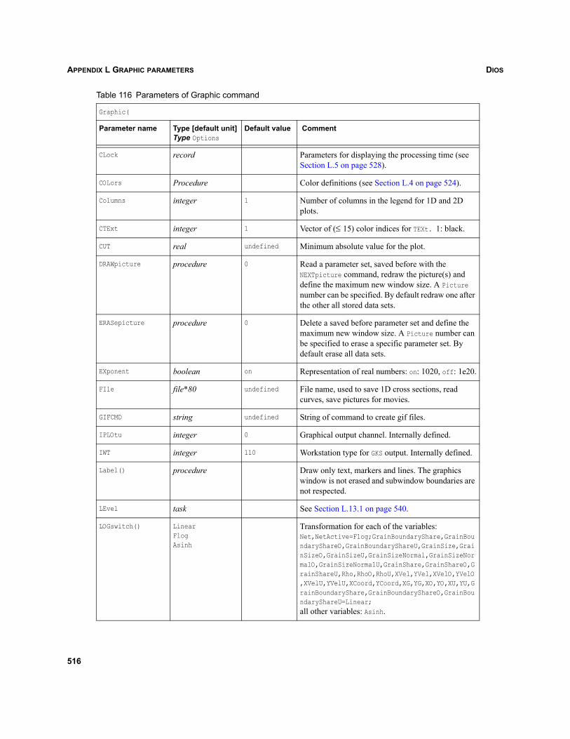
DIOSAPPENDIX L GRAPHIC PARAMETERS
CLock record Parameters for displaying the processing time (see Section L.5 on page 528).
COLors Procedure Color definitions (see Section L.4 on page 524).
Columns integer 1 Number of columns in the legend for 1D and 2D plots.
CTExt integer 1 Vector of (≤ 15) color indices for TEXt. 1: black.
CUT real undefined Minimum absolute value for the plot.
DRAWpicture procedure 0 Read a parameter set, saved before with the NEXTpicture command, redraw the picture(s) and define the maximum new window size. A Picture number can be specified. By default redraw one after the other all stored data sets.
ERASepicture procedure 0 Delete a saved before parameter set and define the maximum new window size. A Picture number can be specified to erase a specific parameter set. By default erase all data sets.
EXponent boolean on Representation of real numbers: on: 1020, off: 1e20.
FIle file*80 undefined File name, used to save 1D cross sections, read curves, save pictures for movies.
GIFCMD string undefined String of command to create gif files.
IPLOtu integer 0 Graphical output channel. Internally defined.
IWT integer 110 Workstation type for GKS output. Internally defined.
Label() procedure Draw only text, markers and lines. The graphics window is not erased and subwindow boundaries are not respected.
LEvel task See Section L.13.1 on page 540.
LOGswitch() LinearFlogAsinh
Transformation for each of the variables:Net,NetActive=Flog;GrainBoundaryShare,GrainBoundaryShareO,GrainBoundaryShareU,GrainSize,GrainSizeO,GrainSizeU,GrainSizeNormal,GrainSizeNormalO,GrainSizeNormalU,GrainShare,GrainShareO,GrainShareU,Rho,RhoO,RhoU,XVel,YVel,XVelO,YVelO,XVelU,YVelU,XCoord,YCoord,XG,YG,XO,YO,XU,YU,GrainBoundaryShare,GrainBoundaryShareO,GrainBoundaryShareU=Linear;all other variables: Asinh.
Table 116 Parameters of Graphic command
Graphic(
Parameter name Type [default unit]Type Options
Default value Comment
516
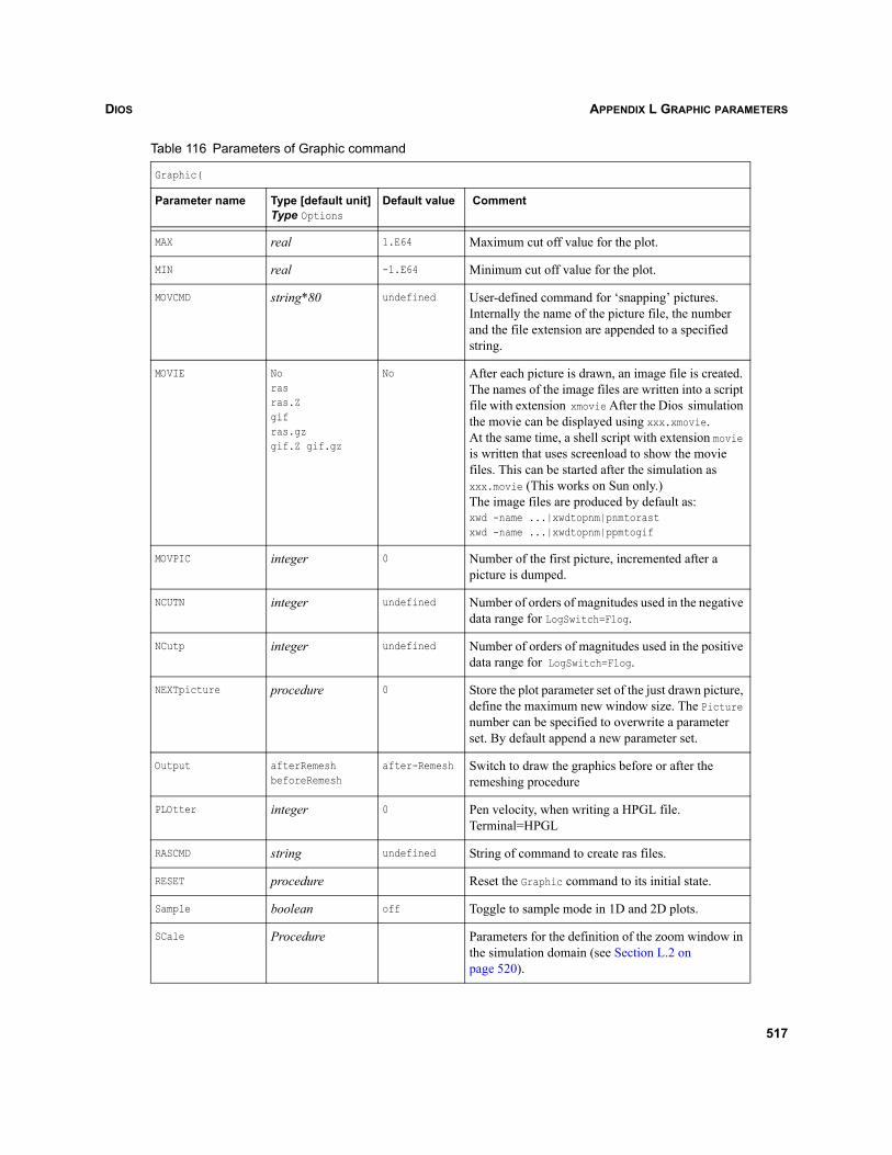
DIOS APPENDIX L GRAPHIC PARAMETERS
MAX real 1.E64 Maximum cut off value for the plot.
MIN real -1.E64 Minimum cut off value for the plot.
MOVCMD string*80 undefined User-defined command for ‘snapping’ pictures. Internally the name of the picture file, the number and the file extension are appended to a specified string.
MOVIE Norasras.Zgifras.gz gif.Z gif.gz
No After each picture is drawn, an image file is created. The names of the image files are written into a script file with extension xmovie After the Dios simulation the movie can be displayed using xxx.xmovie.At the same time, a shell script with extension movie is written that uses screenload to show the movie files. This can be started after the simulation as xxx.movie (This works on Sun only.)The image files are produced by default as:xwd -name ...|xwdtopnm|pnmtorastxwd -name ...|xwdtopnm|ppmtogif
MOVPIC integer 0 Number of the first picture, incremented after a picture is dumped.
NCUTN integer undefined Number of orders of magnitudes used in the negative data range for LogSwitch=Flog.
NCutp integer undefined Number of orders of magnitudes used in the positive data range for LogSwitch=Flog.
NEXTpicture procedure 0 Store the plot parameter set of the just drawn picture, define the maximum new window size. The Picture number can be specified to overwrite a parameter set. By default append a new parameter set.
Output afterRemeshbeforeRemesh
after-Remesh Switch to draw the graphics before or after the remeshing procedure
PLOtter integer 0 Pen velocity, when writing a HPGL file.Terminal=HPGL
RASCMD string undefined String of command to create ras files.
RESET procedure Reset the Graphic command to its initial state.
Sample boolean off Toggle to sample mode in 1D and 2D plots.
SCale Procedure Parameters for the definition of the zoom window in the simulation domain (see Section L.2 on page 520).
Table 116 Parameters of Graphic command
Graphic(
Parameter name Type [default unit]Type Options
Default value Comment
517
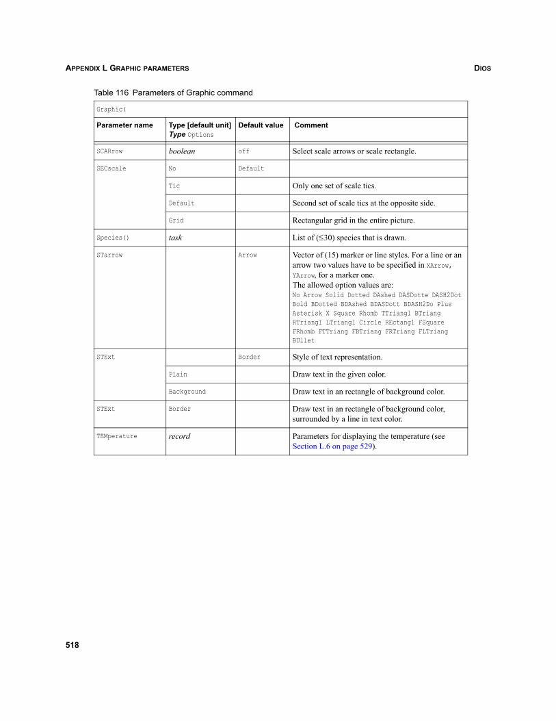
DIOSAPPENDIX L GRAPHIC PARAMETERS
SCARrow boolean off Select scale arrows or scale rectangle.
SECscale No Default
Tic Only one set of scale tics.
Default Second set of scale tics at the opposite side.
Grid Rectangular grid in the entire picture.
Species() task List of (≤30) species that is drawn.
STarrow Arrow Vector of (15) marker or line styles. For a line or an arrow two values have to be specified in XArrow, YArrow, for a marker one.The allowed option values are:No Arrow Solid Dotted DAshed DASDotte DASH2Dot Bold BDotted BDAshed BDASDott BDASH2Do Plus Asterisk X Square Rhomb TTriangl BTriang RTriangl LTriangl Circle REctangl FSquare FRhomb FTTriang FBTriang FRTriang FLTriang BUllet
STExt Border Style of text representation.
Plain Draw text in the given color.
Background Draw text in an rectangle of background color.
STExt Border Draw text in an rectangle of background color, surrounded by a line in text color.
TEMperature record Parameters for displaying the temperature (see Section L.6 on page 529).
Table 116 Parameters of Graphic command
Graphic(
Parameter name Type [default unit]Type Options
Default value Comment
518
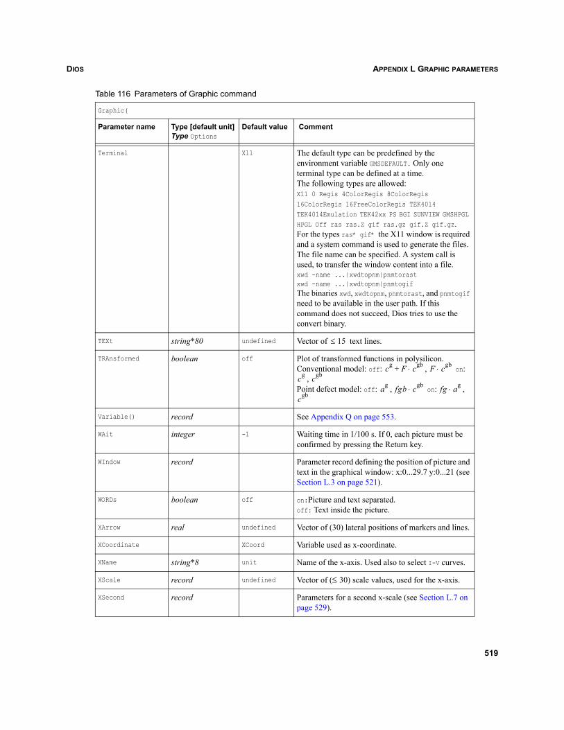
DIOS APPENDIX L GRAPHIC PARAMETERS
Terminal X11 The default type can be predefined by the environment variable GMSDEFAULT. Only one terminal type can be defined at a time. The following types are allowed:X11 0 Regis 4ColorRegis 8ColorRegis 16ColorRegis 16FreeColorRegis TEK4014 TEK4014Emulation TEK42xx PS BGI SUNVIEW GMSHPGL HPGL Off ras ras.Z gif ras.gz gif.Z gif.gz.For the types ras* gif* the X11 window is required and a system command is used to generate the files. The file name can be specified. A system call is used, to transfer the window content into a file.xwd -name ...|xwdtopnm|pnmtorastxwd -name ...|xwdtopnm|pnmtogifThe binaries xwd, xwdtopnm, pnmtorast, and pnmtogif need to be available in the user path. If this command does not succeed, Dios tries to use the convert binary.
TEXt string*80 undefined Vector of text lines.
TRAnsformed boolean off Plot of transformed functions in polysilicon.Conventional model: off: , on:
, Point defect model: off: , on: ,
Variable() record See Appendix Q on page 553.
WAit integer -1 Waiting time in 1/100 s. If 0, each picture must be confirmed by pressing the Return key.
WIndow record Parameter record defining the position of picture and text in the graphical window: x:0...29.7 y:0...21 (see Section L.3 on page 521).
WORDs boolean off on:Picture and text separated.off: Text inside the picture.
XArrow real undefined Vector of (30) lateral positions of markers and lines.
XCoordinate XCoord Variable used as x-coordinate.
XName string*8 unit Name of the x-axis. Used also to select I-V curves.
XScale record undefined Vector of (≤ 30) scale values, used for the x-axis.
XSecond record Parameters for a second x-scale (see Section L.7 on page 529).
Table 116 Parameters of Graphic command
Graphic(
Parameter name Type [default unit]Type Options
Default value Comment
15≤
cg F cgb⋅+ F cgb⋅cg cgb
ag fgb cgb⋅ fg ag⋅cgb
519
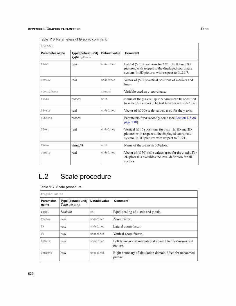
DIOSAPPENDIX L GRAPHIC PARAMETERS
L.2 Scale procedure
XText real undefined Lateral (≤ 15) positions for TEXt. In 1D and 2D pictures, with respect to the displayed coordinate system. In 3D pictures with respect to 0...29.7.
YArrow real undefined Vector of (≤ 30) vertical positions of markers and lines.
YCoordinate YCoord Variable used as y-coordinate.
YName record unit Name of the y-axis. Up to 5 names can be specified to select I-V curves. The last 4 names are undefined.
YScale real undefined Vector of (≤ 30) scale values, used for the y-axis.
YSecond record Parameters for a second y-scale (see Section L.8 on page 530).
YText real undefined Vertical (≤ 15) positions for TEXt. In 1D and 2D pictures with respect to the displayed coordinate system. In 3D pictures with respect to 0...21.
ZName string*8 unit Name of the z-axis in 3D-plots.
ZScale real undefined Vector of (≤ 30) scale values, used for the z-axis. For 2D plots this overrides the level definition for all species.
Table 117 Scale procedure
Graphic(Scale(
Parameter name
Type [default unit]Type Options
Default value Comment
Equal boolean on Equal scaling of x-axis and y-axis.
Factor real undefined Zoom factor.
FX real undefined Lateral zoom factor.
FY real undefined Vertical zoom factor.
GXLeft real undefined Left boundary of simulation domain. Used for unzoomed picture.
GXRight real undefined Right boundary of simulation domain. Used for unzoomed picture.
Table 116 Parameters of Graphic command
Graphic(
Parameter name Type [default unit]Type Options
Default value Comment
520
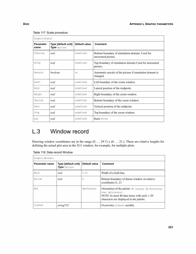
DIOS APPENDIX L GRAPHIC PARAMETERS
L.3 Window recordDrawing window coordinates are in the range (0. … 29.7) x (0. … 21.). These are relative lengths fordefining the actual plot area in the X11 window, for example, for multiple plots.
GYBottom real undefined Bottom boundary of simulation domain. Used for unzoomed picture.
GYTop real undefined Top boundary of simulation domain.Used for unzoomed picture.
Rescale boolean on Automatic rescale of the picture if simulation domain is changed.
XLeft real undefined Left boundary of the zoom window.
Xmid real undefined Lateral position of the midpoint.
XRight real undefined Right boundary of the zoom window.
YBottom real undefined Bottom boundary of the zoom window.
Ymid real undefined Vertical position of the midpoint.
YTop real undefined Top boundary of the zoom window.
Zyx real undefined Ratio FY/FX.
Table 118 Data record Window
Graphic(Window(
Parameter name Type [default unit]Type Options
Default value Comment
BOLd real 0.15 Width of a bold line.
Bottom real 0. Bottom boundary of drawn window in relative coordinates 0...21
BOX UpOrLateral Orientation of the palette No Lateral Up Horizontal Down UpOrLateral.NOTE At most 40 data items with each characters are displayed in the palette.
DISPLAY string*32 Overwrites DISPLAY variable.
Table 117 Scale procedure
Graphic(Scale(
Parameter name
Type [default unit]Type Options
Default value Comment
20≤
521
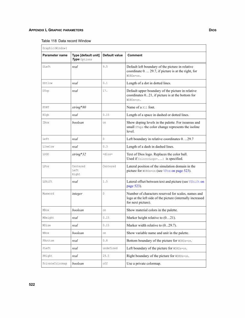
DIOSAPPENDIX L GRAPHIC PARAMETERS
DLeft real 9.5 Default left boundary of the picture in relative coordinate 0. ... 29.7, if picture is at the right, for WORDs=on.
DOtlow real 0.1 Length of a dot in dotted lines.
DTop real 17. Default upper boundary of the picture in relative coordinates 0...21, if picture is at the bottom for WORDs=on.
FONT string*80 Name of a X11 font.
HIgh real 0.15 Length of a space in dashed or dotted lines.
IBox boolean on Show doping levels in the palette. For isoareas and small STeps the color change represents the isoline level.
Left real 0 Left boundary in relative coordinates 0. ...29.7
LInelow real 0.3 Length of a dash in dashed lines.
LOGO string*32 =dios= Text of Dios logo. Replaces the color ball.Used if Colors(Logo=...) is specified.
LPos CenteredLeftRight
Centered Lateral position of the simulation domain in the picture for WORDs=on (see VPos on page 523).
LShift real 1.5 Lateral offset between text and picture (see VShift on page 523).
Maxword integer 0 Number of characters reserved for scales, names and logo at the left side of the picture (internally increased for next picture).
MBox boolean on Show material colors in the palette.
MHeight real 0.15 Marker height relative to (0…21).
MSize real 0.15 Marker width relative to (0...29.7).
NBox boolean on Show variable name and unit in the palette.
PBottom real 0.8 Bottom boundary of the picture for WORDs=on.
PLeft real undefined Left boundary of the picture for WORDs=on.
PRight real 29.5 Right boundary of the picture for WORDs=on.
PrivateColormap boolean off Use a private colormap.
Table 118 Data record Window
Graphic(Window(
Parameter name Type [default unit]Type Options
Default value Comment
522
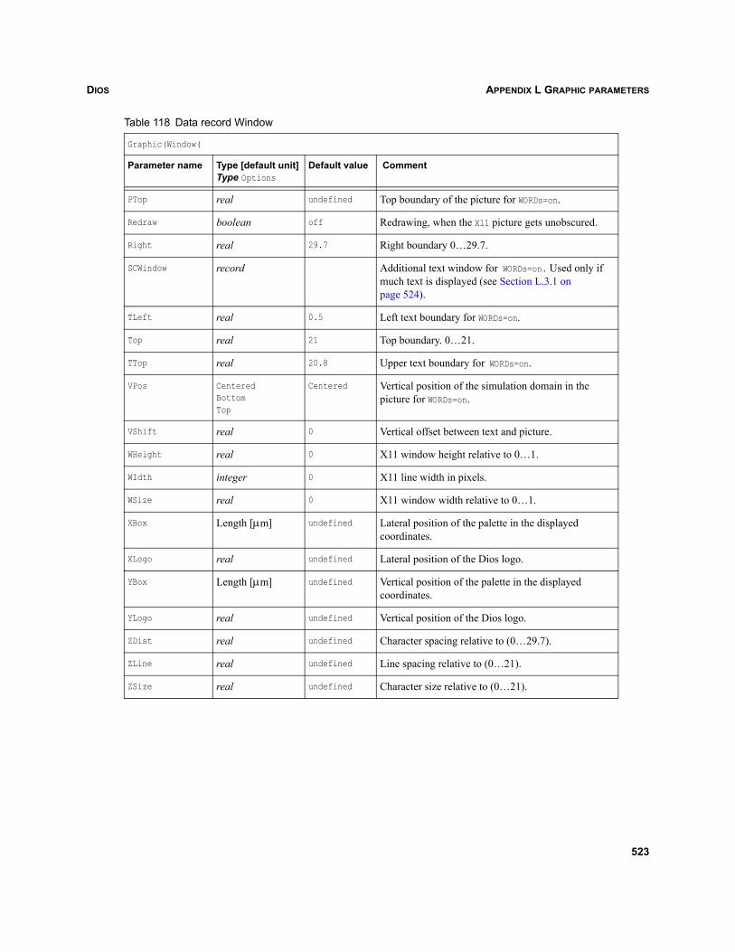
DIOS APPENDIX L GRAPHIC PARAMETERS
PTop real undefined Top boundary of the picture for WORDs=on.
Redraw boolean off Redrawing, when the X11 picture gets unobscured.
Right real 29.7 Right boundary 0…29.7.
SCWindow record Additional text window for WORDs=on. Used only if much text is displayed (see Section L.3.1 on page 524).
TLeft real 0.5 Left text boundary for WORDs=on.
Top real 21 Top boundary. 0…21.
TTop real 20.8 Upper text boundary for WORDs=on.
VPos CenteredBottomTop
Centered Vertical position of the simulation domain in the picture for WORDs=on.
VShift real 0 Vertical offset between text and picture.
WHeight real 0 X11 window height relative to 0…1.
WIdth integer 0 X11 line width in pixels.
WSize real 0 X11 window width relative to 0…1.
XBox Length [μm] undefined Lateral position of the palette in the displayed coordinates.
XLogo real undefined Lateral position of the Dios logo.
YBox Length [μm] undefined Vertical position of the palette in the displayed coordinates.
YLogo real undefined Vertical position of the Dios logo.
ZDist real undefined Character spacing relative to (0…29.7).
ZLine real undefined Line spacing relative to (0…21).
ZSize real undefined Character size relative to (0…21).
Table 118 Data record Window
Graphic(Window(
Parameter name Type [default unit]Type Options
Default value Comment
523
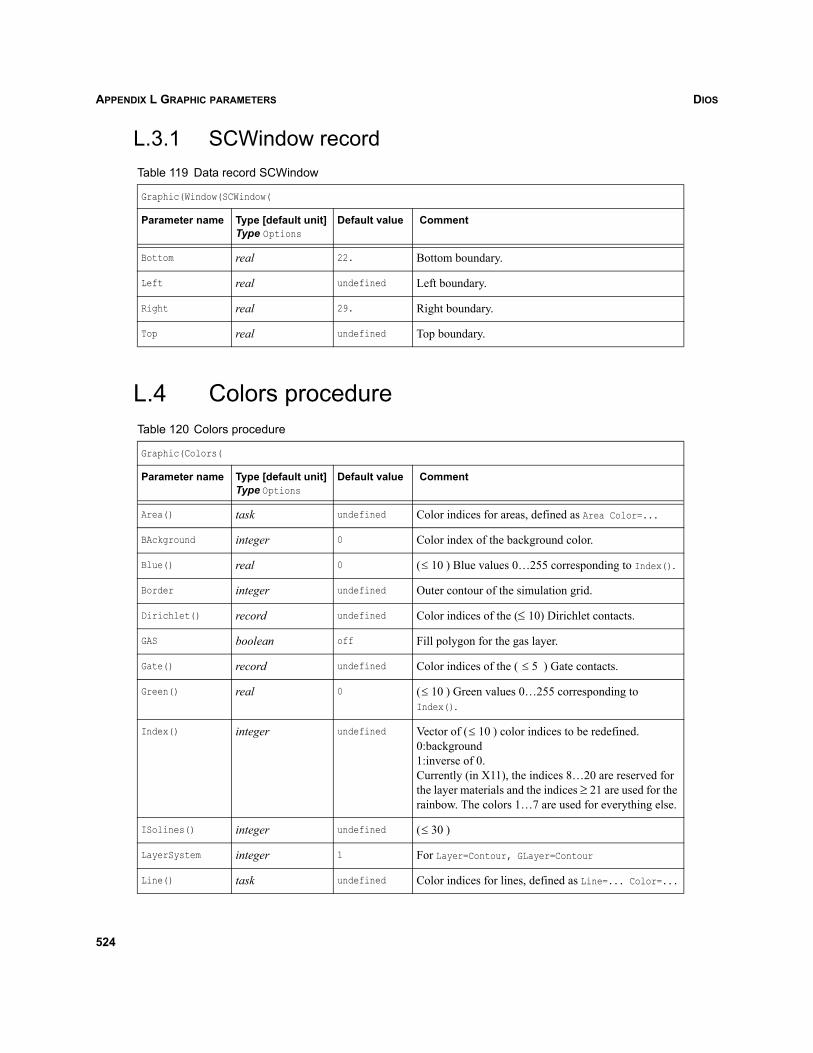
DIOSAPPENDIX L GRAPHIC PARAMETERS
L.3.1 SCWindow record
L.4 Colors procedure
Table 119 Data record SCWindow
Graphic(Window(SCWindow(
Parameter name Type [default unit]Type Options
Default value Comment
Bottom real 22. Bottom boundary.
Left real undefined Left boundary.
Right real 29. Right boundary.
Top real undefined Top boundary.
Table 120 Colors procedure
Graphic(Colors(
Parameter name Type [default unit]Type Options
Default value Comment
Area() task undefined Color indices for areas, defined as Area Color=...
BAckground integer 0 Color index of the background color.
Blue() real 0 ( ) Blue values 0…255 corresponding to Index().
Border integer undefined Outer contour of the simulation grid.
Dirichlet() record undefined Color indices of the (≤ 10) Dirichlet contacts.
GAS boolean off Fill polygon for the gas layer.
Gate() record undefined Color indices of the ( ) Gate contacts.
Green() real 0 ( ) Green values 0…255 corresponding to Index().
Index() integer undefined Vector of ( ) color indices to be redefined.0:background 1:inverse of 0. Currently (in X11), the indices 8…20 are reserved for the layer materials and the indices ≥ 21 are used for the rainbow. The colors 1…7 are used for everything else.
ISolines() integer undefined ( )
LayerSystem integer 1 For Layer=Contour, GLayer=Contour
Line() task undefined Color indices for lines, defined as Line=... Color=...
10≤
5≤
10≤
10≤
30≤
524
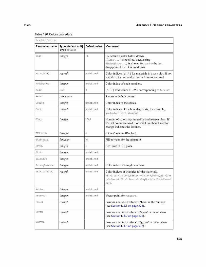
DIOS APPENDIX L GRAPHIC PARAMETERS
Logo integer -1 By default a color ball is drawn.If Logo=... is specified, a text string Window(Logo=...) is drawn, for Logo=0 the text disappears, for -1 it is not drawn.
Material() record undefined Color indices ( ) for materials in Layer plot. If not specified, the internally reserved colors are used.
NodeNumber integer undefined Color index of node numbers.
Red() real 0 ( ) Red values 0…255 corresponding to Index().
Reset procedure Return to default colors.
Scales integer undefined Color index of the scales.
Sort record undefined Color indices of the boundary sorts, for example, gra(colors(sort(siox=5))).
STeps integer 1000 Number of color steps in isoline and isoarea plots. If >50 all colors are used. For small numbers the color change indicates the isolines.
SUBottom integer 4 ‘Down’ side in 3D–plots.
Substrate boolean on Fill polygon for the substrate.
SUTop integer 1 ‘Up’ side in 3D–plots.
TExt integer undefined
TRiangle integer undefined
TriangleNumber integer undefined Color index of triangle numbers.
TRIMaterial() record undefined Color indices of triangles for the materials. Si:=1,Ox:=7,Ni:=2,Resist:=6,Al:=3,Po:=4,MS:=2,Me:=5,Gas:=4,SG:=1,Rand:=11,OxyN:=5,IsoX:=4,Ceramic:=1.
Vector integer undefined
Vector1 integer undefined Vector point for VSHape=0.
XBLUE record Position and RGB values of ‘blue’ in the rainbow (see Section L.4.1 on page 526).
XCYAN record Position and RGB values of ‘cyan’ in the rainbow (see Section L.4.2 on page 526).
XGREEN record Position and RGB values of ‘green’ in the rainbow (see Section L.4.3 on page 527).
Table 120 Colors procedure
Graphic(Colors(
Parameter name Type [default unit]Type Options
Default value Comment
14≤
10≤
525
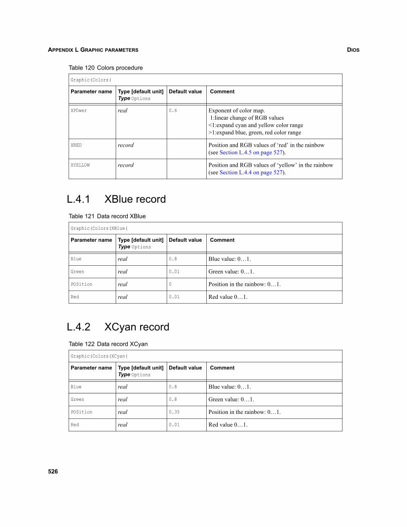
DIOSAPPENDIX L GRAPHIC PARAMETERS
L.4.1 XBlue record
L.4.2 XCyan record
XPOwer real 0.6 Exponent of color map. 1:linear change of RGB values<1:expand cyan and yellow color range>1:expand blue, green, red color range
XRED record Position and RGB values of ‘red’ in the rainbow (see Section L.4.5 on page 527).
XYELLOW record Position and RGB values of ‘yellow’ in the rainbow (see Section L.4.4 on page 527).
Table 121 Data record XBlue
Graphic(Colors(XBlue(
Parameter name Type [default unit]Type Options
Default value Comment
Blue real 0.8 Blue value: 0…1.
Green real 0.01 Green value: 0…1.
POSition real 0 Position in the rainbow: 0…1.
Red real 0.01 Red value 0…1.
Table 122 Data record XCyan
Graphic(Colors(XCyan(
Parameter name Type [default unit]Type Options
Default value Comment
Blue real 0.8 Blue value: 0…1.
Green real 0.8 Green value: 0…1.
POSition real 0.35 Position in the rainbow: 0…1.
Red real 0.01 Red value 0…1.
Table 120 Colors procedure
Graphic(Colors(
Parameter name Type [default unit]Type Options
Default value Comment
526
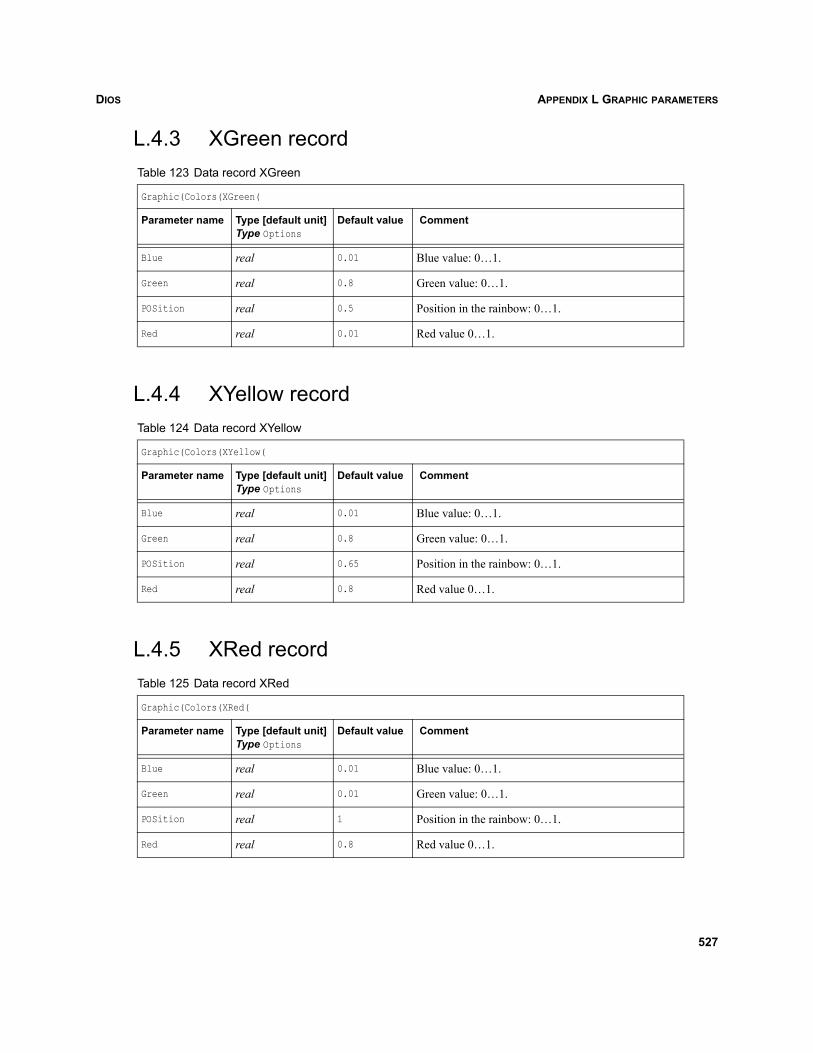
DIOS APPENDIX L GRAPHIC PARAMETERS
L.4.3 XGreen record
L.4.4 XYellow record
L.4.5 XRed record
Table 123 Data record XGreen
Graphic(Colors(XGreen(
Parameter name Type [default unit]Type Options
Default value Comment
Blue real 0.01 Blue value: 0…1.
Green real 0.8 Green value: 0…1.
POSition real 0.5 Position in the rainbow: 0…1.
Red real 0.01 Red value 0…1.
Table 124 Data record XYellow
Graphic(Colors(XYellow(
Parameter name Type [default unit]Type Options
Default value Comment
Blue real 0.01 Blue value: 0…1.
Green real 0.8 Green value: 0…1.
POSition real 0.65 Position in the rainbow: 0…1.
Red real 0.8 Red value 0…1.
Table 125 Data record XRed
Graphic(Colors(XRed(
Parameter name Type [default unit]Type Options
Default value Comment
Blue real 0.01 Blue value: 0…1.
Green real 0.01 Green value: 0…1.
POSition real 1 Position in the rainbow: 0…1.
Red real 0.8 Red value 0…1.
527
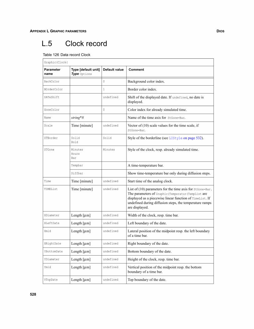
DIOSAPPENDIX L GRAPHIC PARAMETERS
L.5 Clock recordTable 126 Data record Clock
Graphic(Clock(
Parameter name
Type [default unit]Type Options
Default value Comment
BackColor 0 Background color index.
BOrderColor 1 Border color index.
DATeShift undefined Shift of the displayed date. If undefined, no date is displayed.
GoneColor 0 Color index for already simulated time.
Name string*8 Name of the time axis for StGone=Bar.
Scale Time [minute] undefined Vector of (10) scale values for the time scale, if StGone=Bar.
STBorder SolidBold
Solid Style of the borderline (see LIStyle on page 532).
STGone MinutesHoursBar
Minutes Style of the clock, resp. already simulated time.
Tempbar A time-temperature bar.
Diffbar Show time-temperature bar only during diffusion steps.
Time Time [minute] undefined Start time of the analog clock.
TIMEList Time [minute] undefined List of (10) parameters for the time axis for StGone=Bar.The parameters of Graphic(Temperatur(TempList are displayed as a piecewise linear function of TimeList. If undefined during diffusion steps, the temperature ramps are displayed.
XDiameter Length [μm] undefined Width of the clock, resp. time bar.
XLeftDate Length [μm] undefined Left boundary of the date.
Xmid Length [μm] undefined Lateral position of the midpoint resp. the left boundary of a time bar.
XRightDate Length [μm] undefined Right boundary of the date.
YBottomDate Length [μm] undefined Bottom boundary of the date.
YDiameter Length [μm] undefined Height of the clock, resp. time bar.
Ymid Length [μm] undefined Vertical position of the midpoint resp. the bottom boundary of a time bar.
YTopDate Length [μm] undefined Top boundary of the date.
528
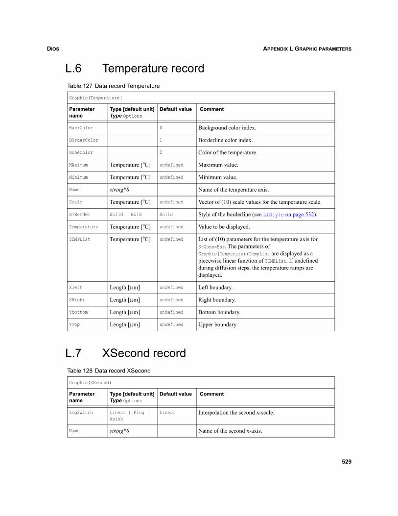
DIOS APPENDIX L GRAPHIC PARAMETERS
L.6 Temperature record
L.7 XSecond record
Table 127 Data record Temperature
Graphic(Temperature(
Parameter name
Type [default unit]Type Options
Default value Comment
BackColor 0 Background color index.
BOrderColor 1 Borderline color index.
GoneColor 2 Color of the temperature.
MAximum Temperature [oC] undefined Maximum value.
Minimum Temperature [oC] undefined Minimum value.
Name string*8 Name of the temperature axis.
Scale Temperature [oC] undefined Vector of (10) scale values for the temperature scale.
STBorder Solid | Bold Solid Style of the borderline (see LIStyle on page 532).
Temperature Temperature [oC] undefined Value to be displayed.
TEMPList Temperature [oC] undefined List of (10) parameters for the temperature axis for StGone=Bar. The parameters of Graphic(Temperatur(TempList are displayed as a piecewise linear function of TIMEList. If undefined during diffusion steps, the temperature ramps are displayed.
Xleft Length [μm] undefined Left boundary.
XRight Length [μm] undefined Right boundary.
Ybottom Length [μm] undefined Bottom boundary.
YTop Length [μm] undefined Upper boundary.
Table 128 Data record XSecond
Graphic(XSecond(
Parameter name
Type [default unit]Type Options
Default value Comment
LogSwitch Linear | Flog |Asinh
Linear Interpolation the second x-scale.
Name string*8 Name of the second x-axis.
529
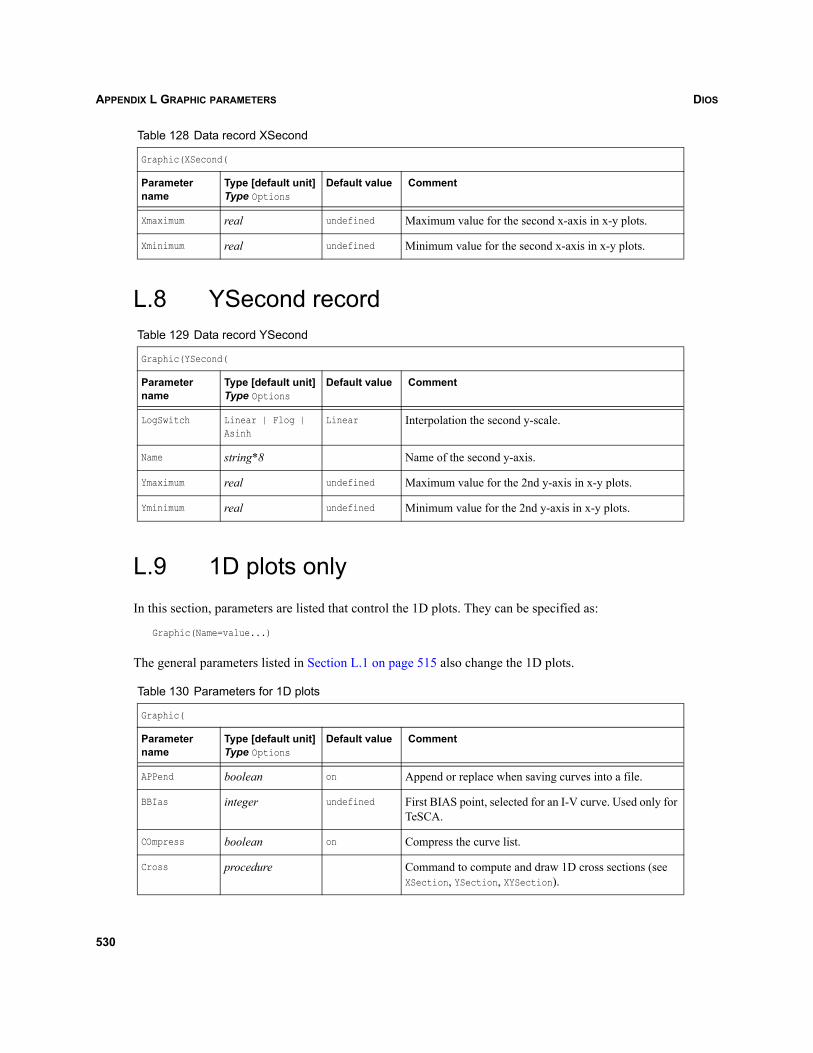
DIOSAPPENDIX L GRAPHIC PARAMETERS
L.8 YSecond record
L.9 1D plots onlyIn this section, parameters are listed that control the 1D plots. They can be specified as:
Graphic(Name=value...)
The general parameters listed in Section L.1 on page 515 also change the 1D plots.
Xmaximum real undefined Maximum value for the second x-axis in x-y plots.
Xminimum real undefined Minimum value for the second x-axis in x-y plots.
Table 129 Data record YSecond
Graphic(YSecond(
Parameter name
Type [default unit]Type Options
Default value Comment
LogSwitch Linear | Flog |Asinh
Linear Interpolation the second y-scale.
Name string*8 Name of the second y-axis.
Ymaximum real undefined Maximum value for the 2nd y-axis in x-y plots.
Yminimum real undefined Minimum value for the 2nd y-axis in x-y plots.
Table 130 Parameters for 1D plots
Graphic(
Parameter name
Type [default unit]Type Options
Default value Comment
APPend boolean on Append or replace when saving curves into a file.
BBIas integer undefined First BIAS point, selected for an I-V curve. Used only for TeSCA.
COmpress boolean on Compress the curve list.
Cross procedure Command to compute and draw 1D cross sections (see XSection, YSection, XYSection).
Table 128 Data record XSecond
Graphic(XSecond(
Parameter name
Type [default unit]Type Options
Default value Comment
530
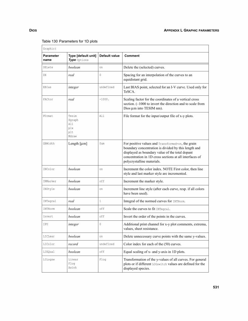
DIOS APPENDIX L GRAPHIC PARAMETERS
DELete boolean on Delete the (selected) curves.
DX real 0 Spacing for an interpolation of the curves to an equidistant grid.
EBIas integer undefined Last BIAS point, selected for an I-V curve. Used only for TeSCA.
FACtor real -1000. Scaling factor for the coordinates of a vertical cross section. (–1000 to invert the direction and to scale from Dios μm into TESIM nm).
FOrmat TesimXgraphAllplxpltMdraw
All File format for the input/output file of x-y plots.
GBWidth Length [μm] 0um For positive values and Transformed=on, the grain boundary concentration is divided by this length and displayed as boundary value of the total dopant concentration in 1D cross sections at all interfaces of polycrystalline materials.
INColor boolean on Increment the color index. NOTE First color, then line style and last marker style are incremented.
INMarker boolean off Increment the marker style.
INStyle boolean on Increment line style (after each curve, resp. if all colors have been used).
INTegral real 1 Integral of the normed curves for INTNorm.
INTNorm boolean off Scale the curves to fit INTegral.
Invert boolean off Invert the order of the points in the curves.
IPU integer 0 Additional print channel for x-y plot comments, extrema, values, sheet resistance.
LICLear boolean on Delete unnecessary curve points with the same y-values.
LIColor record undefined Color index for each of the (50) curves.
LIEQual boolean off Equal scaling of x- and y-axis in 1D plots.
LILogsw LinearFlogAsinh
Flog Transformation of the y-values of all curves. For general plots or if different LOGswitch values are defined for the displayed species.
Table 130 Parameters for 1D plots
Graphic(
Parameter name
Type [default unit]Type Options
Default value Comment
531
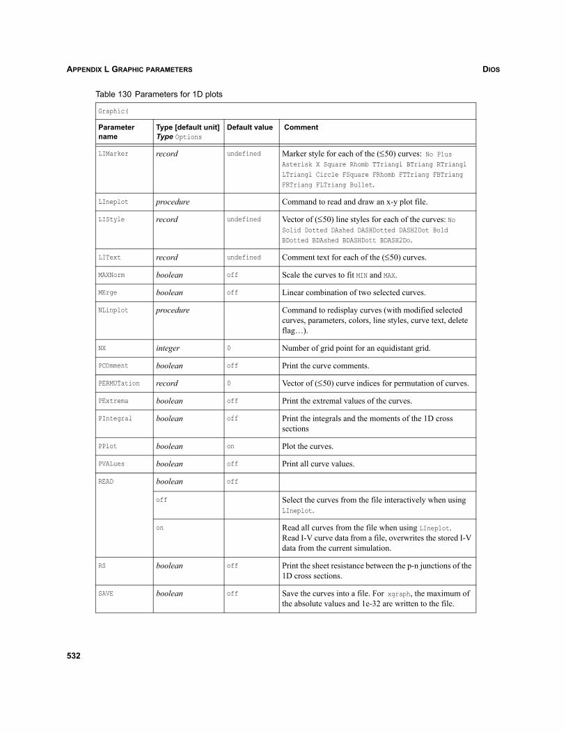
DIOSAPPENDIX L GRAPHIC PARAMETERS
LIMarker record undefined Marker style for each of the (≤50) curves: No Plus Asterisk X Square Rhomb TTriangl BTriang RTriangl LTriangl Circle FSquare FRhomb FTTriang FBTriang FRTriang FLTriang Bullet.
LIneplot procedure Command to read and draw an x-y plot file.
LIStyle record undefined Vector of (≤50) line styles for each of the curves: No Solid Dotted DAshed DASHDotted DASH2Dot Bold BDotted BDAshed BDASHDott BDASH2Do.
LIText record undefined Comment text for each of the (≤50) curves.
MAXNorm boolean off Scale the curves to fit MIN and MAX.
MErge boolean off Linear combination of two selected curves.
NLinplot procedure Command to redisplay curves (with modified selected curves, parameters, colors, line styles, curve text, delete flag…).
NX integer 0 Number of grid point for an equidistant grid.
PCOmment boolean off Print the curve comments.
PERMUTation record 0 Vector of (≤50) curve indices for permutation of curves.
PExtrema boolean off Print the extremal values of the curves.
PIntegral boolean off Print the integrals and the moments of the 1D cross sections
PPlot boolean on Plot the curves.
PVALues boolean off Print all curve values.
READ boolean off
off Select the curves from the file interactively when using LIneplot.
on Read all curves from the file when using LIneplot. Read I-V curve data from a file, overwrites the stored I-V data from the current simulation.
RS boolean off Print the sheet resistance between the p-n junctions of the 1D cross sections.
SAVE boolean off Save the curves into a file. For xgraph, the maximum of the absolute values and 1e-32 are written to the file.
Table 130 Parameters for 1D plots
Graphic(
Parameter name
Type [default unit]Type Options
Default value Comment
532
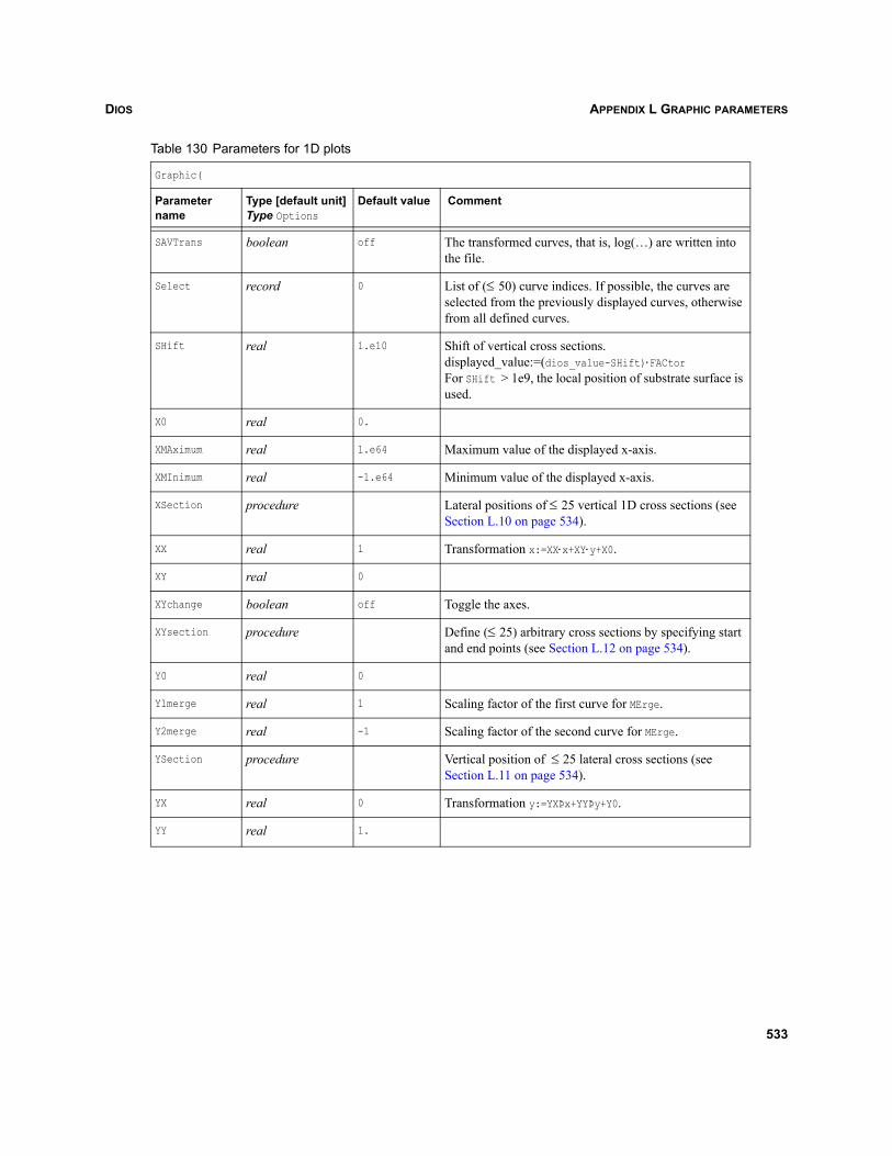
DIOS APPENDIX L GRAPHIC PARAMETERS
SAVTrans boolean off The transformed curves, that is, log(…) are written into the file.
Select record 0 List of (≤ 50) curve indices. If possible, the curves are selected from the previously displayed curves, otherwise from all defined curves.
SHift real 1.e10 Shift of vertical cross sections.displayed_value:=(dios_value-SHift)⋅FACtorFor SHift > 1e9, the local position of substrate surface is used.
X0 real 0.
XMAximum real 1.e64 Maximum value of the displayed x-axis.
XMInimum real -1.e64 Minimum value of the displayed x-axis.
XSection procedure Lateral positions of ≤ 25 vertical 1D cross sections (see Section L.10 on page 534).
XX real 1 Transformation x:=XX⋅x+XY⋅y+X0.
XY real 0
XYchange boolean off Toggle the axes.
XYsection procedure Define (≤ 25) arbitrary cross sections by specifying start and end points (see Section L.12 on page 534).
Y0 real 0
Y1merge real 1 Scaling factor of the first curve for MErge.
Y2merge real -1 Scaling factor of the second curve for MErge.
YSection procedure Vertical position of ≤ 25 lateral cross sections (see Section L.11 on page 534).
YX real 0 Transformation y:=YXÞx+YYÞy+Y0.
YY real 1.
Table 130 Parameters for 1D plots
Graphic(
Parameter name
Type [default unit]Type Options
Default value Comment
533
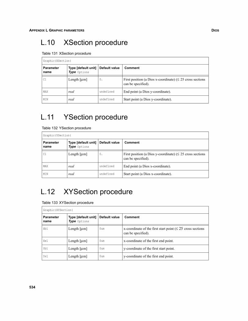
DIOSAPPENDIX L GRAPHIC PARAMETERS
L.10 XSection procedure
L.11 YSection procedure
L.12 XYSection procedure
Table 131 XSection procedure
Graphic(XSection(
Parameter name
Type [default unit]Type Options
Default value Comment
C1 Length [μm] 0. First position (a Dios x-coordinate) (≤ 25 cross sections can be specified).
MAX real undefined End point (a Dios y-coordinate).
MIN real undefined Start point (a Dios y-coordinate).
Table 132 YSection procedure
Graphic(YSection(
Parameter name
Type [default unit]Type Options
Default value Comment
C1 Length [μm] 0. First position (a Dios y-coordinate) (≤ 25 cross sections can be specified).
MAX real undefined End point (a Dios x-coordinate).
MIN real undefined Start point (a Dios x-coordinate).
Table 133 XYSection procedure
Graphic(XYSection(
Parameter name
Type [default unit]Type Options
Default value Comment
Xb1 Length [μm] 0um x-coordinate of the first start point (≤ 25 cross sections can be specified).
Xe1 Length [μm] 0um x-coordinate of the first end point.
Yb1 Length [μm] 0um y-coordinate of the first start point.
Ye1 Length [μm] 0um y-coordinate of the first end point.
534
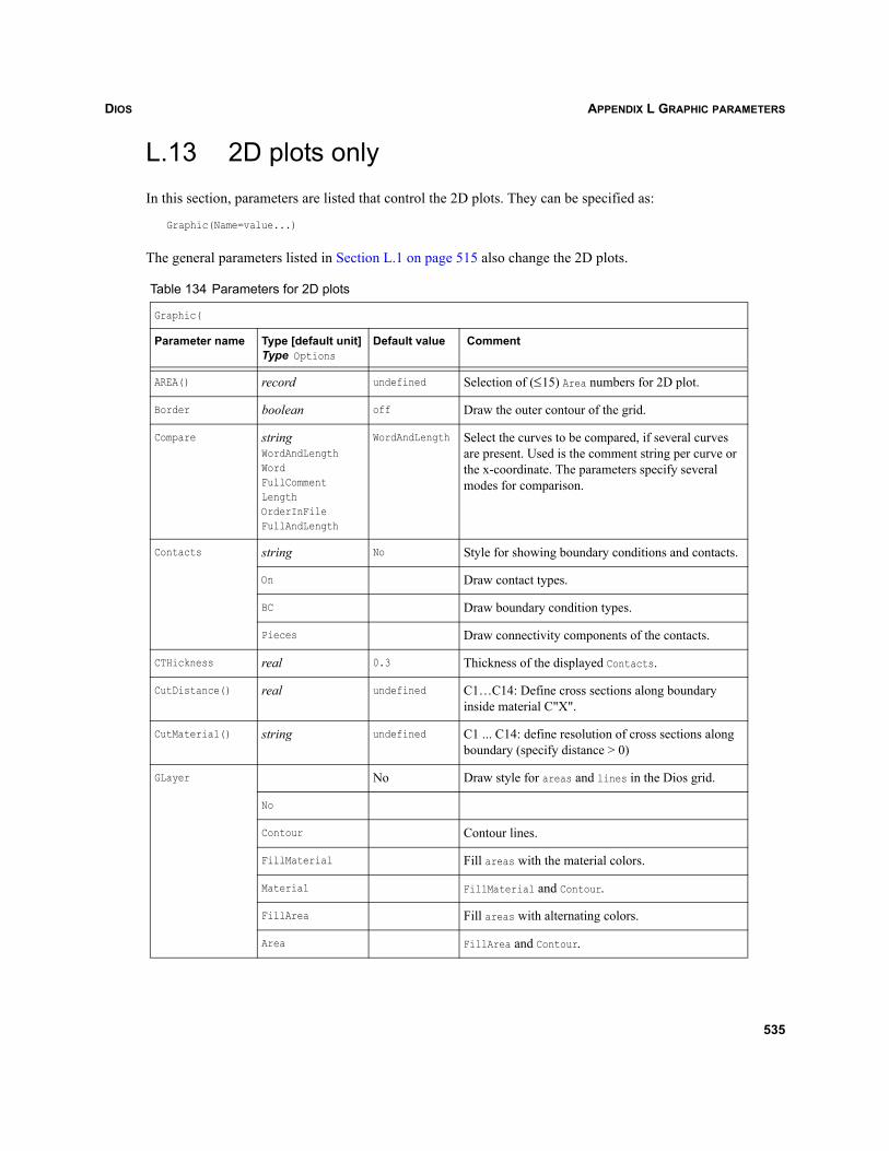
DIOS APPENDIX L GRAPHIC PARAMETERS
L.13 2D plots onlyIn this section, parameters are listed that control the 2D plots. They can be specified as:
Graphic(Name=value...)
The general parameters listed in Section L.1 on page 515 also change the 2D plots.
Table 134 Parameters for 2D plots
Graphic(
Parameter name Type [default unit]Type Options
Default value Comment
AREA() record undefined Selection of (≤15) Area numbers for 2D plot.
Border boolean off Draw the outer contour of the grid.
Compare stringWordAndLengthWordFullCommentLengthOrderInFileFullAndLength
WordAndLength Select the curves to be compared, if several curves are present. Used is the comment string per curve or the x-coordinate. The parameters specify several modes for comparison.
Contacts string No Style for showing boundary conditions and contacts.
On Draw contact types.
BC Draw boundary condition types.
Pieces Draw connectivity components of the contacts.
CTHickness real 0.3 Thickness of the displayed Contacts.
CutDistance() real undefined C1…C14: Define cross sections along boundary inside material C"X".
CutMaterial() string undefined C1 ... C14: define resolution of cross sections along boundary (specify distance > 0)
GLayer No Draw style for areas and lines in the Dios grid.
No
Contour Contour lines.
FillMaterial Fill areas with the material colors.
Material FillMaterial and Contour.
FillArea Fill areas with alternating colors.
Area FillArea and Contour.
535
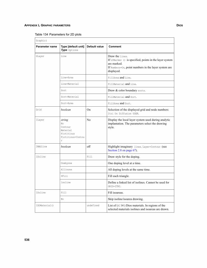
DIOSAPPENDIX L GRAPHIC PARAMETERS
GLayer Line Draw the lines.If LIMarker () is specified, points in the layer system are marked.If Numbers=On, point numbers in the layer system are displayed.
Line+Area FillArea and Line.
Line+Material FillMaterial and Line.
Sort Draw & color boundary sorts.
Sort+Material FillMaterial and Sort.
Sort+Area FillArea and Sort.
Grid boolean On Selection of the displayed grid and node numbers: Itri On Diffusion USER.
ILayer stringNoContourMaterialFictitiousFictitious+Contour
No Display the local layer system used during analytic implantation. The parameters select the drawing style.
IMAGline boolean off Highlight imaginary lines. Layer=Contour (see Section 2.8 on page 67).
ISoline Fill Draw style for the doping.
Onebyone One doping level at a time.
Allinone All doping levels at the same time.
SFill Fill each triangle.
Isoline Define a linked list of isolines. Cannot be used for GRID=ITRI.
ISoline Fill Fill isoareas.
No Skip isoline/isoarea drawing.
ISOMaterial() undefined List of ( ) Dios materials. In regions of the selected materials isolines and isoareas are drawn.
Table 134 Parameters for 2D plots
Graphic(
Parameter name Type [default unit]Type Options
Default value Comment
14≤
536
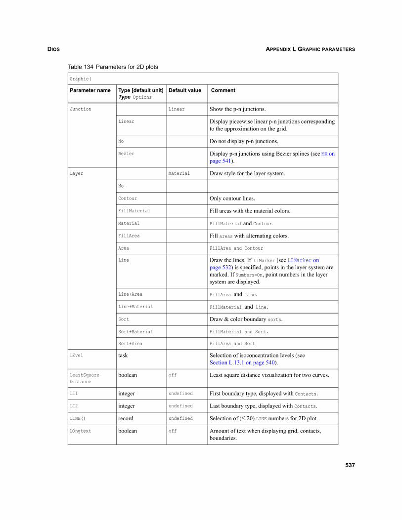
DIOS APPENDIX L GRAPHIC PARAMETERS
Junction Linear Show the p-n junctions.
Linear Display piecewise linear p-n junctions corresponding to the approximation on the grid.
No Do not display p-n junctions.
Bezier Display p-n junctions using Bezier splines (see MX on page 541).
Layer Material Draw style for the layer system.
No
Contour Only contour lines.
FillMaterial Fill areas with the material colors.
Material FillMaterial and Contour.
FillArea Fill areas with alternating colors.
Area FillArea and Contour
Line Draw the lines. If LIMarker (see LIMarker on page 532) is specified, points in the layer system are marked. If Numbers=On, point numbers in the layer system are displayed.
Line+Area FillArea and Line.
Line+Material FillMaterial and Line.
Sort Draw & color boundary sorts.
Sort+Material FillMaterial and Sort.
Sort+Area FillArea and Sort
LEvel task Selection of isoconcentration levels (see Section L.13.1 on page 540).
LeastSquare-Distance
boolean off Least square distance vizualization for two curves.
LI1 integer undefined First boundary type, displayed with Contacts.
LI2 integer undefined Last boundary type, displayed with Contacts.
LINE() record undefined Selection of (≤ 20) LINE numbers for 2D plot.
LOngtext boolean off Amount of text when displaying grid, contacts, boundaries.
Table 134 Parameters for 2D plots
Graphic(
Parameter name Type [default unit]Type Options
Default value Comment
537
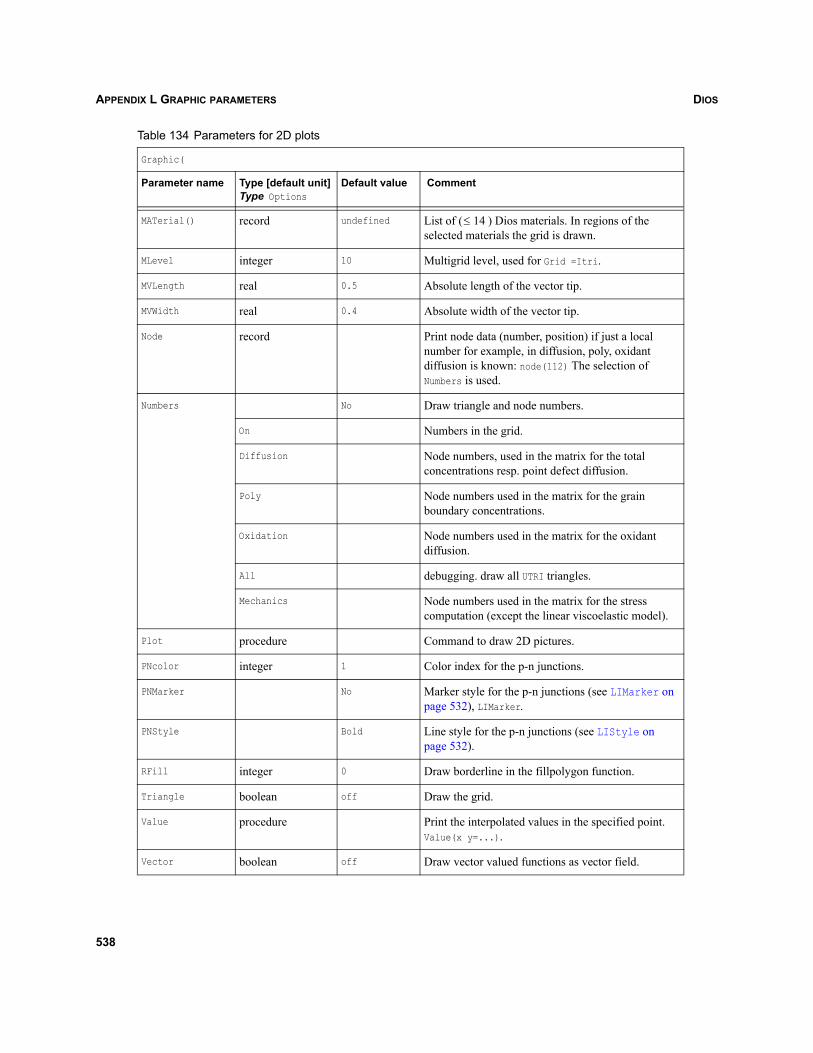
DIOSAPPENDIX L GRAPHIC PARAMETERS
MATerial() record undefined List of ( ) Dios materials. In regions of the selected materials the grid is drawn.
MLevel integer 10 Multigrid level, used for Grid =Itri.
MVLength real 0.5 Absolute length of the vector tip.
MVWidth real 0.4 Absolute width of the vector tip.
Node record Print node data (number, position) if just a local number for example, in diffusion, poly, oxidant diffusion is known: node(112) The selection of Numbers is used.
Numbers No Draw triangle and node numbers.
On Numbers in the grid.
Diffusion Node numbers, used in the matrix for the total concentrations resp. point defect diffusion.
Poly Node numbers used in the matrix for the grain boundary concentrations.
Oxidation Node numbers used in the matrix for the oxidant diffusion.
All debugging. draw all UTRI triangles.
Mechanics Node numbers used in the matrix for the stress computation (except the linear viscoelastic model).
Plot procedure Command to draw 2D pictures.
PNcolor integer 1 Color index for the p-n junctions.
PNMarker No Marker style for the p-n junctions (see LIMarker on page 532), LIMarker.
PNStyle Bold Line style for the p-n junctions (see LIStyle on page 532).
RFill integer 0 Draw borderline in the fillpolygon function.
Triangle boolean off Draw the grid.
Value procedure Print the interpolated values in the specified point. Value(x y=...).
Vector boolean off Draw vector valued functions as vector field.
Table 134 Parameters for 2D plots
Graphic(
Parameter name Type [default unit]Type Options
Default value Comment
14≤
538
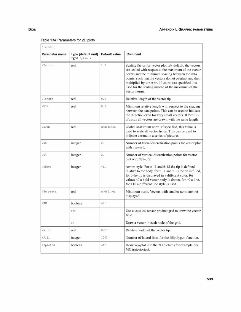
DIOS APPENDIX L GRAPHIC PARAMETERS
VFactor real 1.5 Scaling factor for vector plot. By default, the vectors are scaled with respect to the maximum of the vector norms and the minimum spacing between the data points, such that the vectors do not overlap, and then multiplied by VFactor. If VNOrm was specified it is used for the scaling instead of the maximum of the vector norms.
VLength real 0.4 Relative length of the vector tip.
VMIN real 0.3 Minimum relative length with respect to the spacing between the data points. This can be used to indicate the direction even for very small vectors. If VMIN >= VFactor all vectors are drawn with the same length.
VNOrm real undefined Global Maximum norm. If specified, this value is used to scale all vector fields. This can be used to indicate a trend in a series of pictures.
VNX integer 20 Number of lateral discretization points for vector plot with VSW=off.
VNY integer 20 Number of vertical discretization points for vector plot with VSW=off.
VSHape integer -11 Arrow style. For ± 11 and ± 12 the tip is defined relative to the body, for ± 11 and ± 13 the tip is filled, for 0 the tip is displayed in a different color, for values <0 a bold vector body is drawn, for >0 a line, for >10 a different line style is used.
VSuppress real undefined Minimum norm. Vectors with smaller norm are not displayed.
VSW boolean off
off Use a VNX×VNY tensor product grid to draw the vector field.
on Draw a vector in each node of the grid.
VWidth real 0.23 Relative width of the vector tip.
XFill integer 1000 Number of lateral lines for the fillpolygon function.
XYplot2d boolean off Draw x-y-plot into the 2D picture (for example, for MC trajectories).
Table 134 Parameters for 2D plots
Graphic(
Parameter name Type [default unit]Type Options
Default value Comment
539
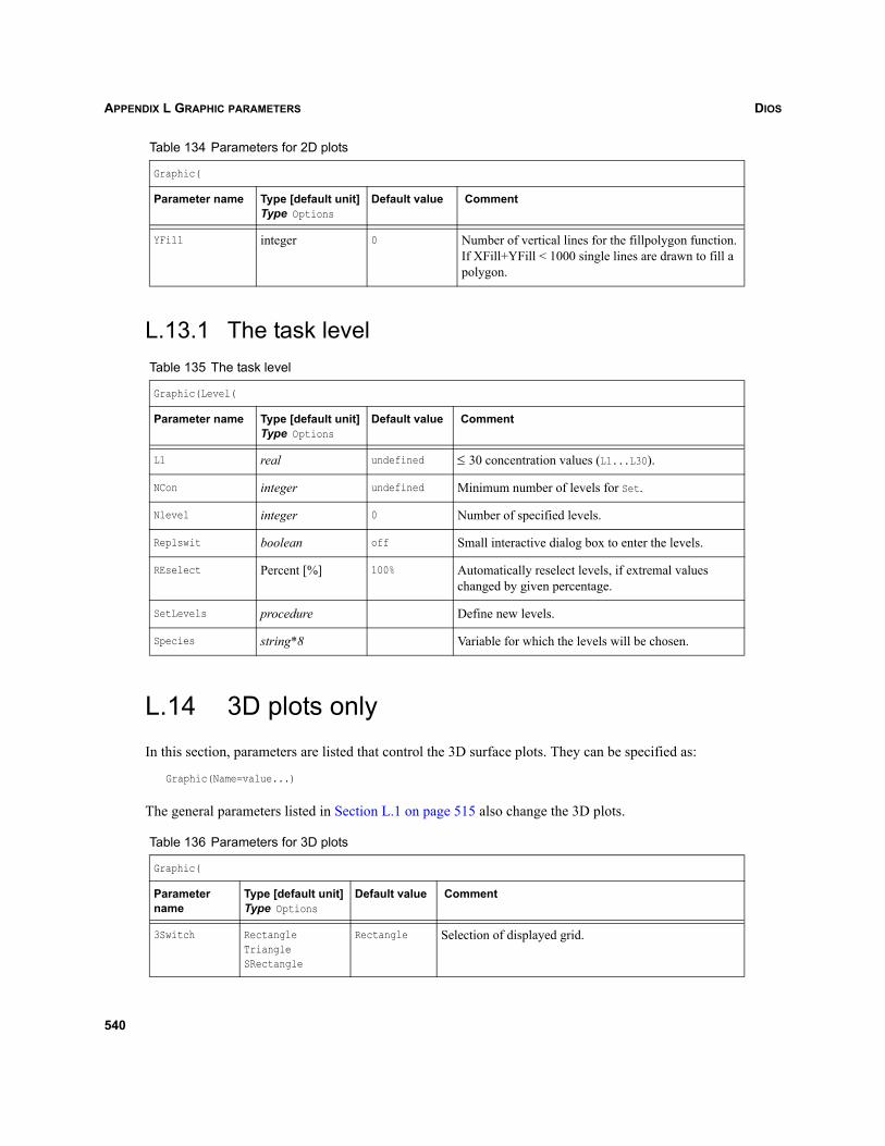
DIOSAPPENDIX L GRAPHIC PARAMETERS
L.13.1 The task level
L.14 3D plots onlyIn this section, parameters are listed that control the 3D surface plots. They can be specified as:
Graphic(Name=value...)
The general parameters listed in Section L.1 on page 515 also change the 3D plots.
YFill integer 0 Number of vertical lines for the fillpolygon function. If XFill+YFill < 1000 single lines are drawn to fill a polygon.
Table 135 The task level
Graphic(Level(
Parameter name Type [default unit]Type Options
Default value Comment
L1 real undefined ≤ 30 concentration values (L1...L30).
NCon integer undefined Minimum number of levels for Set.
Nlevel integer 0 Number of specified levels.
Replswit boolean off Small interactive dialog box to enter the levels.
REselect Percent [%] 100% Automatically reselect levels, if extremal values changed by given percentage.
SetLevels procedure Define new levels.
Species string*8 Variable for which the levels will be chosen.
Table 136 Parameters for 3D plots
Graphic(
Parameter name
Type [default unit]Type Options
Default value Comment
3Switch RectangleTriangleSRectangle
Rectangle Selection of displayed grid.
Table 134 Parameters for 2D plots
Graphic(
Parameter name Type [default unit]Type Options
Default value Comment
540
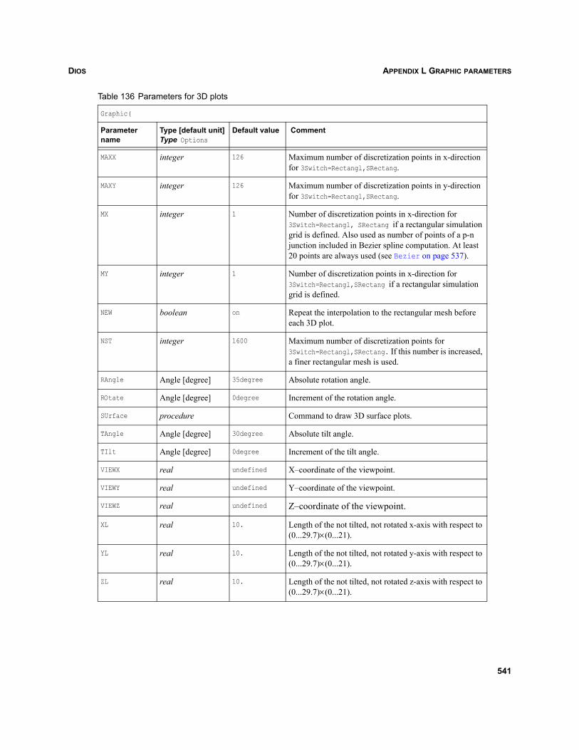
DIOS APPENDIX L GRAPHIC PARAMETERS
MAXX integer 126 Maximum number of discretization points in x-direction for 3Switch=Rectangl,SRectang.
MAXY integer 126 Maximum number of discretization points in y-direction for 3Switch=Rectangl,SRectang.
MX integer 1 Number of discretization points in x-direction for 3Switch=Rectangl, SRectang if a rectangular simulation grid is defined. Also used as number of points of a p-n junction included in Bezier spline computation. At least 20 points are always used (see Bezier on page 537).
MY integer 1 Number of discretization points in x-direction for 3Switch=Rectangl,SRectang if a rectangular simulation grid is defined.
NEW boolean on Repeat the interpolation to the rectangular mesh before each 3D plot.
NST integer 1600 Maximum number of discretization points for 3Switch=Rectangl,SRectang. If this number is increased, a finer rectangular mesh is used.
RAngle Angle [degree] 35degree Absolute rotation angle.
ROtate Angle [degree] 0degree Increment of the rotation angle.
SUrface procedure Command to draw 3D surface plots.
TAngle Angle [degree] 30degree Absolute tilt angle.
TIlt Angle [degree] 0degree Increment of the tilt angle.
VIEWX real undefined X–coordinate of the viewpoint.
VIEWY real undefined Y–coordinate of the viewpoint.
VIEWZ real undefined Z–coordinate of the viewpoint.
XL real 10. Length of the not tilted, not rotated x-axis with respect to (0...29.7)×(0...21).
YL real 10. Length of the not tilted, not rotated y-axis with respect to (0...29.7)×(0...21).
ZL real 10. Length of the not tilted, not rotated z-axis with respect to (0...29.7)×(0...21).
Table 136 Parameters for 3D plots
Graphic(
Parameter name
Type [default unit]Type Options
Default value Comment
541

DIOSAPPENDIX L GRAPHIC PARAMETERS
542
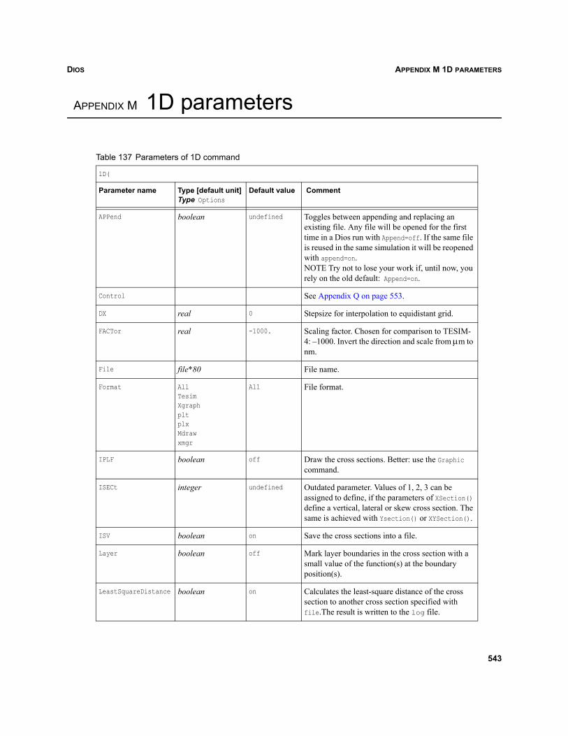
DIOS APPENDIX M 1D PARAMETERS
Dios
APPENDIX M 1D parameters
Table 137 Parameters of 1D command
1D(
Parameter name Type [default unit]Type Options
Default value Comment
APPend boolean undefined Toggles between appending and replacing an existing file. Any file will be opened for the first time in a Dios run with Append=off. If the same file is reused in the same simulation it will be reopened with append=on.NOTE Try not to lose your work if, until now, you rely on the old default: Append=on.
Control See Appendix Q on page 553.
DX real 0 Stepsize for interpolation to equidistant grid.
FACTor real -1000. Scaling factor. Chosen for comparison to TESIM-4: –1000. Invert the direction and scale from μm to nm.
File file*80 File name.
Format AllTesimXgraphpltplxMdrawxmgr
All File format.
IPLF boolean off Draw the cross sections. Better: use the Graphic command.
ISECt integer undefined Outdated parameter. Values of 1, 2, 3 can be assigned to define, if the parameters of XSection() define a vertical, lateral or skew cross section. The same is achieved with Ysection() or XYSection().
ISV boolean on Save the cross sections into a file.
Layer boolean off Mark layer boundaries in the cross section with a small value of the function(s) at the boundary position(s).
LeastSquareDistance boolean on Calculates the least-square distance of the cross section to another cross section specified with file.The result is written to the log file.
543
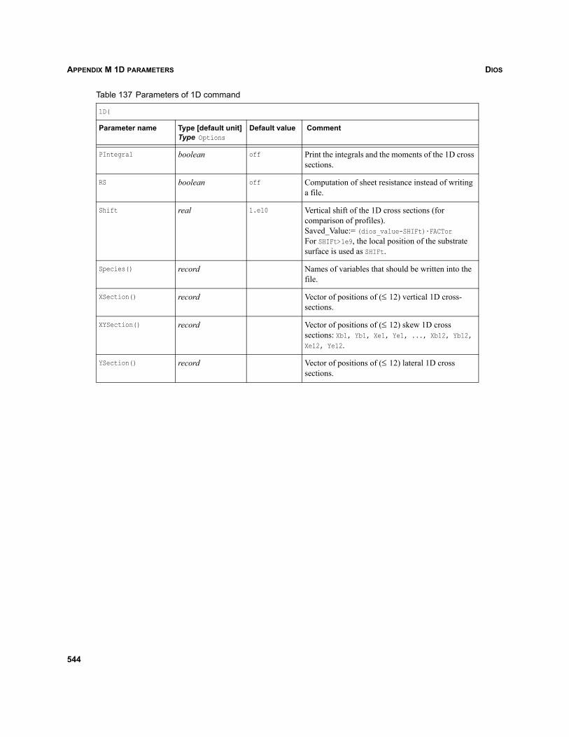
DIOSAPPENDIX M 1D PARAMETERS
PIntegral boolean off Print the integrals and the moments of the 1D cross sections.
RS boolean off Computation of sheet resistance instead of writing a file.
Shift real 1.e10 Vertical shift of the 1D cross sections (for comparison of profiles).Saved_Value:= (dios_value-SHIFt)·FACTorFor SHIFt>1e9, the local position of the substrate surface is used as SHIFt.
Species() record Names of variables that should be written into the file.
XSection() record Vector of positions of (≤ 12) vertical 1D cross- sections.
XYSection() record Vector of positions of (≤ 12) skew 1D cross sections: Xb1, Yb1, Xe1, Ye1, ..., Xb12, Yb12, Xe12, Ye12.
YSection() record Vector of positions of (≤ 12) lateral 1D cross sections.
Table 137 Parameters of 1D command
1D(
Parameter name Type [default unit]Type Options
Default value Comment
544
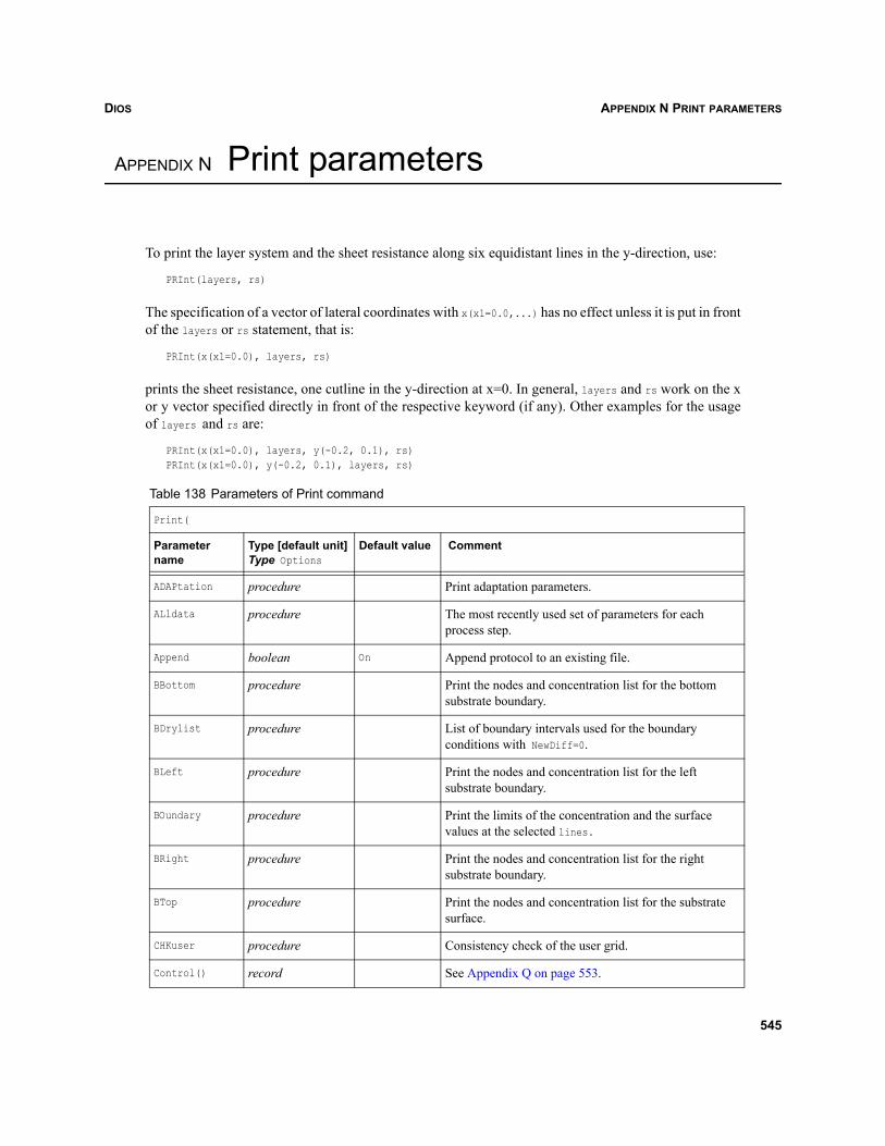
DIOS APPENDIX N PRINT PARAMETERS
Dios
APPENDIX N Print parameters
To print the layer system and the sheet resistance along six equidistant lines in the y-direction, use:
PRInt(layers, rs)
The specification of a vector of lateral coordinates with x(x1=0.0,...) has no effect unless it is put in frontof the layers or rs statement, that is:
PRInt(x(x1=0.0), layers, rs)
prints the sheet resistance, one cutline in the y-direction at x=0. In general, layers and rs work on the xor y vector specified directly in front of the respective keyword (if any). Other examples for the usageof layers and rs are:
PRInt(x(x1=0.0), layers, y(-0.2, 0.1), rs)PRInt(x(x1=0.0), y(-0.2, 0.1), layers, rs)
Table 138 Parameters of Print command
Print(
Parameter name
Type [default unit]Type Options
Default value Comment
ADAPtation procedure Print adaptation parameters.
ALldata procedure The most recently used set of parameters for each process step.
Append boolean On Append protocol to an existing file.
BBottom procedure Print the nodes and concentration list for the bottom substrate boundary.
BDrylist procedure List of boundary intervals used for the boundary conditions with NewDiff=0.
BLeft procedure Print the nodes and concentration list for the left substrate boundary.
BOundary procedure Print the limits of the concentration and the surface values at the selected lines.
BRight procedure Print the nodes and concentration list for the right substrate boundary.
BTop procedure Print the nodes and concentration list for the substrate surface.
CHKuser procedure Consistency check of the user grid.
Control() record See Appendix Q on page 553.
545
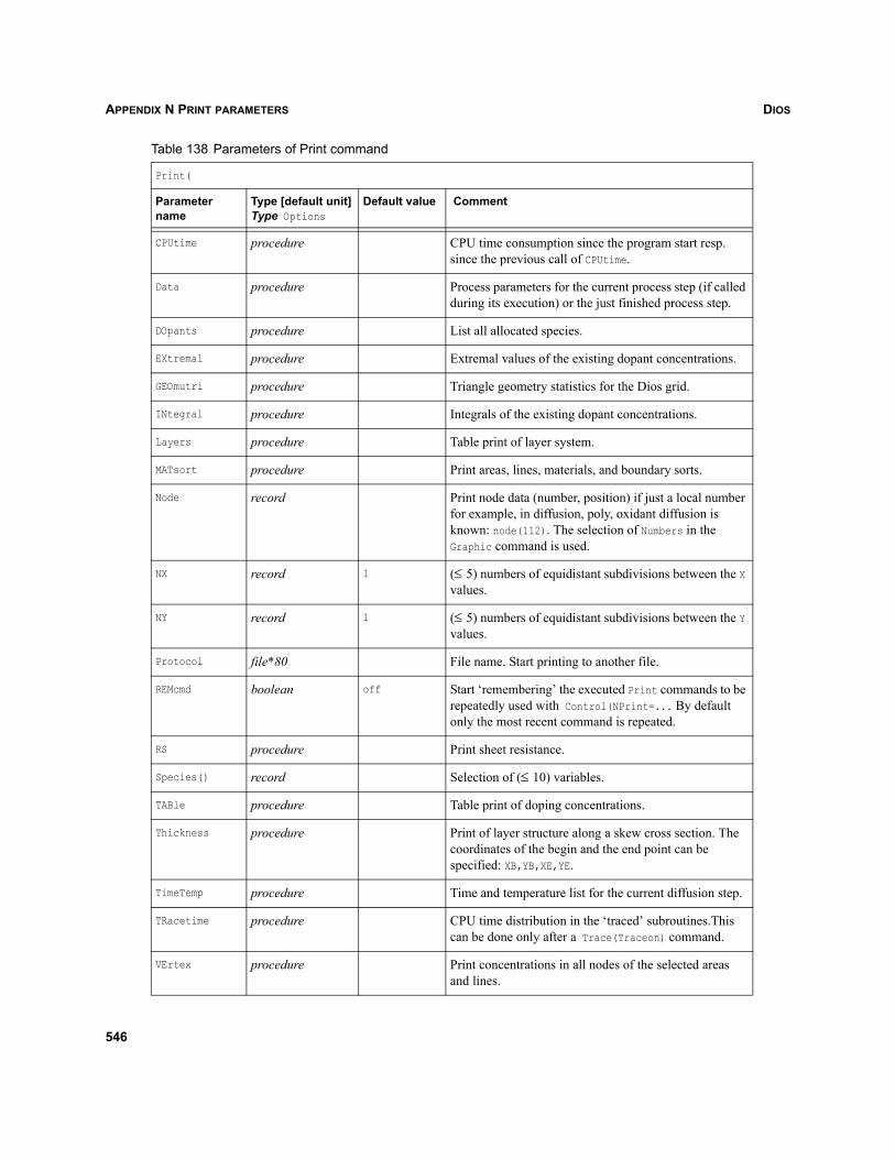
DIOSAPPENDIX N PRINT PARAMETERS
CPUtime procedure CPU time consumption since the program start resp. since the previous call of CPUtime.
Data procedure Process parameters for the current process step (if called during its execution) or the just finished process step.
DOpants procedure List all allocated species.
EXtremal procedure Extremal values of the existing dopant concentrations.
GEOmutri procedure Triangle geometry statistics for the Dios grid.
INtegral procedure Integrals of the existing dopant concentrations.
Layers procedure Table print of layer system.
MATsort procedure Print areas, lines, materials, and boundary sorts.
Node record Print node data (number, position) if just a local number for example, in diffusion, poly, oxidant diffusion is known: node(112). The selection of Numbers in the Graphic command is used.
NX record 1 (≤ 5) numbers of equidistant subdivisions between the X values.
NY record 1 (≤ 5) numbers of equidistant subdivisions between the Y values.
Protocol file*80 File name. Start printing to another file.
REMcmd boolean off Start ‘remembering’ the executed Print commands to be repeatedly used with Control(NPrint=... By default only the most recent command is repeated.
RS procedure Print sheet resistance.
Species() record Selection of (≤ 10) variables.
TABle procedure Table print of doping concentrations.
Thickness procedure Print of layer structure along a skew cross section. The coordinates of the begin and the end point can be specified: XB,YB,XE,YE.
TimeTemp procedure Time and temperature list for the current diffusion step.
TRacetime procedure CPU time distribution in the ‘traced’ subroutines.This can be done only after a Trace(Traceon) command.
VErtex procedure Print concentrations in all nodes of the selected areas and lines.
Table 138 Parameters of Print command
Print(
Parameter name
Type [default unit]Type Options
Default value Comment
546

DIOS APPENDIX N PRINT PARAMETERS
WAit integer -1 Waiting time in 1/100 s. If 0 each print has to be confirmed by pressing the Return key.
X record Vector of (≤6) lateral coordinates for the layer system and table print.
Y record Vector of (≤6) vertical coordinates for the layer system and table print.
Table 138 Parameters of Print command
Print(
Parameter name
Type [default unit]Type Options
Default value Comment
547

DIOSAPPENDIX N PRINT PARAMETERS
548
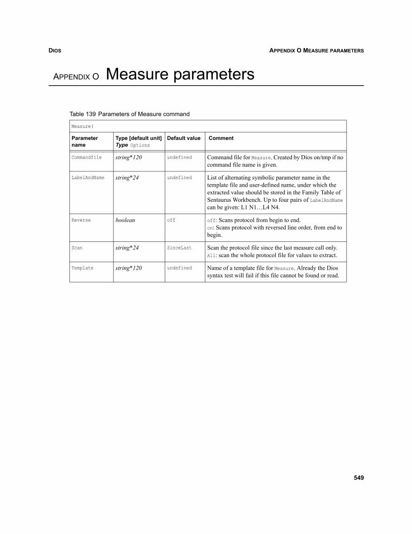
DIOS APPENDIX O MEASURE PARAMETERS
Dios
APPENDIX O Measure parameters
Table 139 Parameters of Measure command
Measure(
Parameter name
Type [default unit]Type Options
Default value Comment
Commandfile string*120 undefined Command file for Measure. Created by Dios on/tmp if no command file name is given.
LabelAndName string*24 undefined List of alternating symbolic parameter name in the template file and user-defined name, under which the extracted value should be stored in the Family Table of Sentaurus Workbench. Up to four pairs of LabelAndName can be given: L1 N1…L4 N4.
Reverse boolean off off: Scans protocol from begin to end.on: Scans protocol with reversed line order, from end to begin.
Scan string*24 SinceLast Scan the protocol file since the last measure call only. All: scan the whole protocol file for values to extract.
Template string*120 undefined Name of a template file for Measure. Already the Dios syntax test will fail if this file cannot be found or read.
549

DIOSAPPENDIX O MEASURE PARAMETERS
550
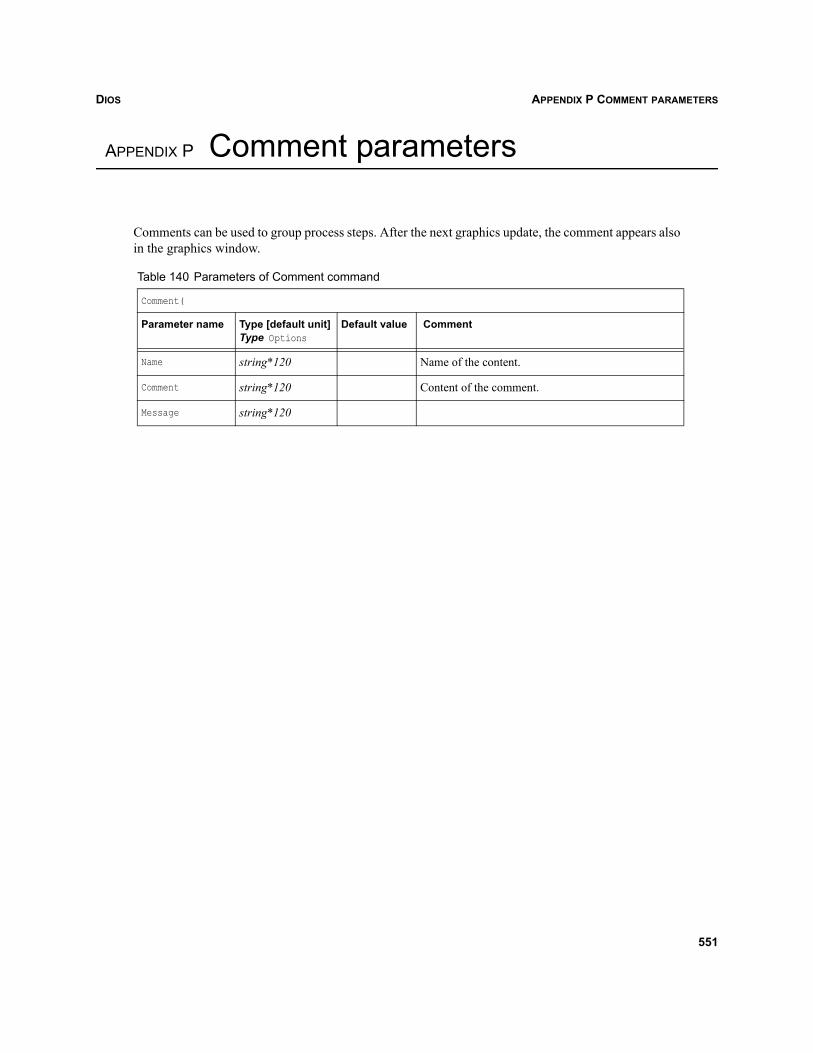
DIOS APPENDIX P COMMENT PARAMETERS
Dios
APPENDIX P Comment parameters
Comments can be used to group process steps. After the next graphics update, the comment appears alsoin the graphics window.
Table 140 Parameters of Comment command
Comment(
Parameter name Type [default unit]Type Options
Default value Comment
Name string*120 Name of the content.
Comment string*120 Content of the comment.
Message string*120
551

DIOSAPPENDIX P COMMENT PARAMETERS
552
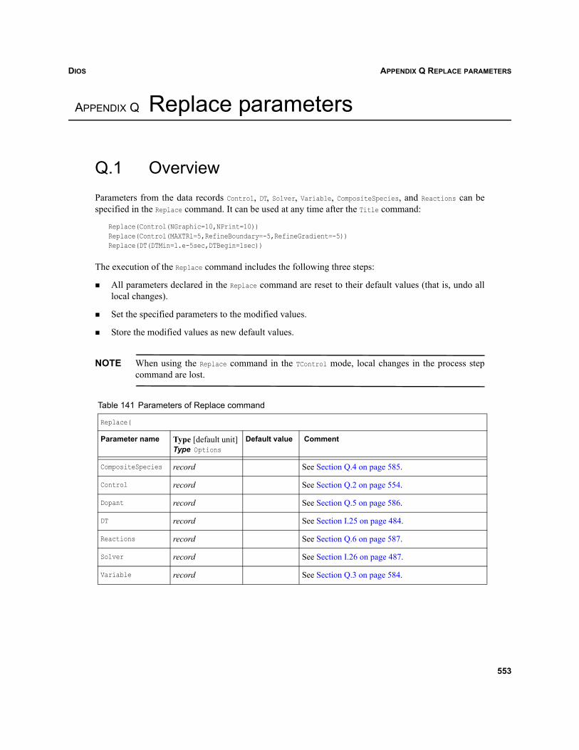
DIOS APPENDIX Q REPLACE PARAMETERS
Dios
APPENDIX Q Replace parameters
Q.1 OverviewParameters from the data records Control, DT, Solver, Variable, CompositeSpecies, and Reactions can bespecified in the Replace command. It can be used at any time after the Title command:
Replace(Control(NGraphic=10,NPrint=10))Replace(Control(MAXTRl=5,RefineBoundary=-5,RefineGradient=-5))Replace(DT(DTMin=1.e-5sec,DTBegin=1sec))
The execution of the Replace command includes the following three steps:
All parameters declared in the Replace command are reset to their default values (that is, undo alllocal changes).
Set the specified parameters to the modified values.
Store the modified values as new default values.
NOTE When using the Replace command in the TControl mode, local changes in the process stepcommand are lost.
Table 141 Parameters of Replace command
Replace(
Parameter name Type [default unit]Type Options
Default value Comment
CompositeSpecies record See Section Q.4 on page 585.
Control record See Section Q.2 on page 554.
Dopant record See Section Q.5 on page 586.
DT record See Section I.25 on page 484.
Reactions record See Section Q.6 on page 587.
Solver record See Section I.26 on page 487.
Variable record See Section Q.3 on page 584.
553
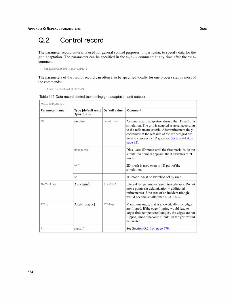
DIOSAPPENDIX Q REPLACE PARAMETERS
Q.2 Control recordThe parameter record Control is used for general control purposes, in particular, to specify data for thegrid adaptation. The parameters can be specified in the Replace command at any time after the Titlecommand:
Replace(Control(name=value))
The parameters of the Control record can often also be specified locally for one process step in most ofthe commands:
Diffusion(Control(LPRot=2))
Table 142 Data record control (controlling grid adaptation and output)
Replace(Control(
Parameter name Type [default unit]Type Options
Default value Comment
1D boolean undefined Automatic grid adaptation during the 1D part of a simulation. The grid is adapted as usual according to the refinement criteria. After refinement the y-coordinate at the left side of the refined grid are used to construct a 1D grid (see Section 4.4.4 on page 92).
undefined Dios uses 1D mode until the first mask inside the simulation domain appears. the it switches to 2D mode.
off 2D-mesh is used even in 1D part of the simulation.
on 1D mode. Must be switched off by user.
AbsTriArea Area [μm2] 1.e-8um2 Internal test parameter. Small triangle area. Do not move points (in delaunization + additional refinements) if the area of an incident triangle would become smaller than AbsTriArea.
AFLip Angle [degree] 178degr Maximum angle, that is allowed, after the edges are flipped. If the edge flipping would lead to larger (but compensated) angles, the edges are not flipped, since otherwise a ‘hole’ in the grid would be created.
Al record See Section Q.2.1 on page 579.
554
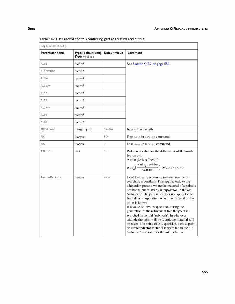
DIOS APPENDIX Q REPLACE PARAMETERS
AlAl record See Section Q.2.2 on page 581.
AlCeramic record
AlGas record
AlIsoX record
AlMe record
AlMS record
AlOxyN record
AlPo record
AlSG record
ANGstroem Length [μm] 1e-4um Internal test length.
AR1 integer 500 First area in a Print command.
AR2 integer 1 Last area in a Print command.
ASHdiff real 1. Reference value for the differences of the asinh for MASS=6.A triangle is refined if:
AssumeMaterial integer -999 Used to specify a dummy material number in searching algorithms. This applies only to the adaptation process where the material of a point is not know, but found by interpolation in the old ‘submesh.’ The parameter does not apply to the final data interpolation, when the material of the point is known.If a value of –999 is specified, during the generation of the refinement tree the point is searched in the old ‘submesh’. In whatever triangle the point will be found, the material will be taken. If a value of 0 is specified, a close point of semiconductor material is searched in the old ‘submesh’ and used for the interpolation.
Table 142 Data record control (controlling grid adaptation and output)
Replace(Control(
Parameter name Type [default unit]Type Options
Default value Comment
maxijciasinh cjasinh–
ASHdiff------------------------------------------⎝ ⎠
⎛ ⎞ 100% IVER 0>>
555
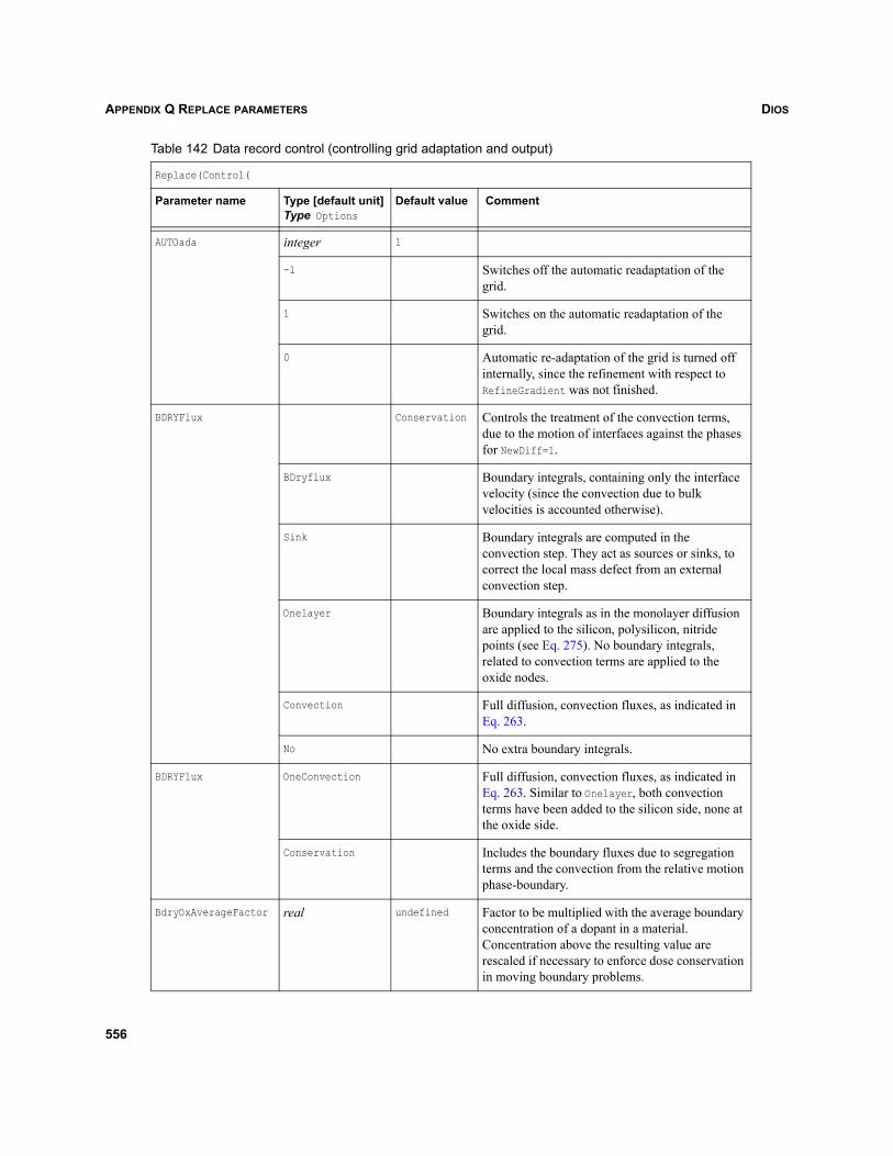
DIOSAPPENDIX Q REPLACE PARAMETERS
AUTOada integer 1
-1 Switches off the automatic readaptation of the grid.
1 Switches on the automatic readaptation of the grid.
0 Automatic re-adaptation of the grid is turned off internally, since the refinement with respect to RefineGradient was not finished.
BDRYFlux Conservation Controls the treatment of the convection terms, due to the motion of interfaces against the phases for NewDiff=1.
BDryflux Boundary integrals, containing only the interface velocity (since the convection due to bulk velocities is accounted otherwise).
Sink Boundary integrals are computed in the convection step. They act as sources or sinks, to correct the local mass defect from an external convection step.
Onelayer Boundary integrals as in the monolayer diffusion are applied to the silicon, polysilicon, nitride points (see Eq. 275). No boundary integrals, related to convection terms are applied to the oxide nodes.
Convection Full diffusion, convection fluxes, as indicated in Eq. 263.
No No extra boundary integrals.
BDRYFlux OneConvection Full diffusion, convection fluxes, as indicated in Eq. 263. Similar to Onelayer, both convection terms have been added to the silicon side, none at the oxide side.
Conservation Includes the boundary fluxes due to segregation terms and the convection from the relative motion phase-boundary.
BdryOxAverageFactor real undefined Factor to be multiplied with the average boundary concentration of a dopant in a material. Concentration above the resulting value are rescaled if necessary to enforce dose conservation in moving boundary problems.
Table 142 Data record control (controlling grid adaptation and output)
Replace(Control(
Parameter name Type [default unit]Type Options
Default value Comment
556
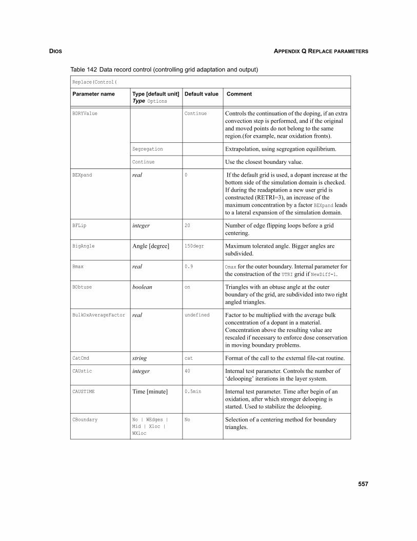
DIOS APPENDIX Q REPLACE PARAMETERS
BDRYValue Continue Controls the continuation of the doping, if an extra convection step is performed, and if the original and moved points do not belong to the same region.(for example, near oxidation fronts).
Segregation Extrapolation, using segregation equilibrium.
Continue Use the closest boundary value.
BEXpand real 0 If the default grid is used, a dopant increase at the bottom side of the simulation domain is checked. If during the readaptation a new user grid is constructed (RETRI=3), an increase of the maximum concentration by a factor BEXpand leads to a lateral expansion of the simulation domain.
BFLip integer 20 Number of edge flipping loops before a grid centering.
BigAngle Angle [degree] 150degr Maximum tolerated angle. Bigger angles are subdivided.
Bmax real 0.9 Omax for the outer boundary. Internal parameter for the construction of the UTRI grid if NewDiff=1.
BObtuse boolean on Triangles with an obtuse angle at the outer boundary of the grid, are subdivided into two right angled triangles.
BulkOxAverageFactor real undefined Factor to be multiplied with the average bulk concentration of a dopant in a material. Concentration above the resulting value are rescaled if necessary to enforce dose conservation in moving boundary problems.
CatCmd string cat Format of the call to the external file-cat routine.
CAUstic integer 40 Internal test parameter. Controls the number of ‘delooping’ iterations in the layer system.
CAUSTIME Time [minute] 0.5min Internal test parameter. Time after begin of an oxidation, after which stronger delooping is started. Used to stabilize the delooping.
CBoundary No | WEdges |Mid | Xloc | WXloc
No Selection of a centering method for boundary triangles.
Table 142 Data record control (controlling grid adaptation and output)
Replace(Control(
Parameter name Type [default unit]Type Options
Default value Comment
557
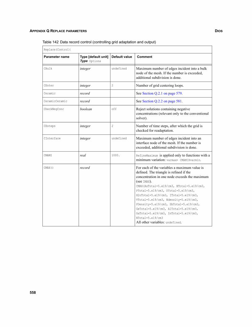
DIOSAPPENDIX Q REPLACE PARAMETERS
CBulk integer undefined Maximum number of edges incident into a bulk node of the mesh. If the number is exceeded, additional subdivision is done.
CEnter integer 2 Number of grid centering loops.
Ceramic record See Section Q.2.1 on page 579.
CeramicCeramic record See Section Q.2.2 on page 581.
CheckNegConc boolean off Reject solutions containing negative concentrations (relevant only to the conventional solver).
CHsteps integer 2 Number of time steps, after which the grid is checked for readaptation.
CInterface integer undefined Maximum number of edges incident into an interface node of the mesh. If the number is exceeded, additional subdivision is done.
CMAMI real 1000. RefineMaximum is applied only to functions with a minimum variation: varmax> CMAMIÞvarmin.
CMAX() record For each of the variables a maximum value is defined. The triangle is refined if the concentration in one node exceeds the maximum (see IMAX).CMAX(AsTotal=5.e19/cm3, BTotal=5.e19/cm3, PTotal=5.e19/cm3, OTotal=5.e19/cm3, H2oTotal=5.e19/cm3, ITotal=5.e19/cm3, VTotal=5.e19/cm3, Ndensity=5.e19/cm3, PDensity=5.e19/cm3, SbTotal=5.e19/cm3, GeTotal=5.e19/cm3, AlTotal=5.e19/cm3, GaTotal=5.e19/cm3, InTotal=5.e19/cm3, NTotal=5.e19/cm3 All other variables: undefined.
Table 142 Data record control (controlling grid adaptation and output)
Replace(Control(
Parameter name Type [default unit]Type Options
Default value Comment
558
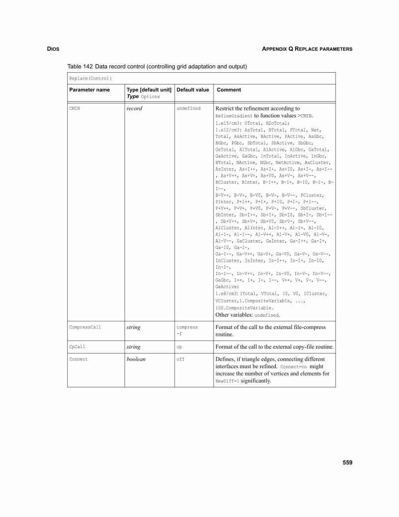
DIOS APPENDIX Q REPLACE PARAMETERS
CMIN record undefined Restrict the refinement according to RefineGradient to function values >CMIN. 1.e15/cm3: OTotal, H2oTotal;1.e12/cm3: AsTotal, BTotal, PTotal, Net, Total, AsActive, BActive, PActive, AsGbc, BGbc, PGbc, SbTotal, SbActive, SbGbc, GeTotal, AlTotal, AlActive, AlGbc, GaTotal, GaActive, GaGbc, InTotal, InActive, InGbc, NTotal, NActive, NGbc, NetActive, AsCluster, AsInter, As+I++, As+I+, As+I0, As+I-, As+I--, As+V++, As+V+, As+V0, As+V-, As+V--, BCluster, BInter, B-I++, B-I+, B-I0, B-I-, B-I--, B-V++, B-V+, B-V0, B-V-, B-V--, PCluster, PInter, P+I++, P+I+, P+I0, P+I-, P+I--, P+V++, P+V+, P+V0, P+V-, P+V--, SbCluster, SbInter, Sb+I++, Sb+I+, Sb+I0, Sb+I-, Sb+I--, Sb+V++, Sb+V+, Sb+V0, Sb+V-, Sb+V--, AlCluster, AlInter, Al-I++, Al-I+, Al-I0, Al-I-, Al-I--, Al-V++, Al-V+, Al-V0, Al-V-, Al-V--, GaCluster, GaInter, Ga-I++, Ga-I+, Ga-I0, Ga-I-, Ga-I--, Ga-V++, Ga-V+, Ga-V0, Ga-V-, Ga-V--, InCluster, InInter, In-I++, In-I+, In-I0, In-I-, In-I--, In-V++, In-V+, In-V0, In-V-, In-V--, GeGbc, I++, I+, I-, I--, V++, V+, V-, V--, GeActive;1.e8/cm3: ITotal, VTotal, I0, V0, ICluster, VCluster,1.CompositeVariable, ..., 100.CompositeVariable.Other variables: undefined.
CompressCall string compress-f
Format of the call to the external file-compress routine.
CpCall string cp Format of the call to the external copy-file routine.
Connect boolean off Defines, if triangle edges, connecting different interfaces must be refined. Connect=on might increase the number of vertices and elements for NewDiff=1 significantly.
Table 142 Data record control (controlling grid adaptation and output)
Replace(Control(
Parameter name Type [default unit]Type Options
Default value Comment
559
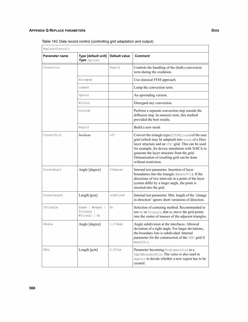
DIOSAPPENDIX Q REPLACE PARAMETERS
Convection Regrid Controls the handling of the (bulk) convection term during the oxidation.
Nolumped Use classical FEM approach.
Lumped Lump the convection term.
Upwind An upwinding version.
Without Disregard any convection.
Outside Perform a separate convection step outside the diffusion step. In numeric tests, this method provided the best results.
Regrid Build a new mesh
ConvertGrid boolean off Convert the triangle type (ITYPET, zone) of the user grid (which may be adapted) into areas of a Dios layer structure and an UTRI grid. This can be used for example, for device simulation with TeSCA to generate the layer structure from the grid. Delaunization of resulting grid can be done without restriction.
CornerAngle Angle [degree] 15degree Internal test parameter. Insertion of layer boundaries into the triangle. (NewDiff=1). If the directions of two intervals in a point of the layer system differ by a larger angle, the point is inserted into the grid.
CornerLength Length [μm] undefined Internal test parameter. Min. length of the ‘change in direction’ ignore short variations of direction.
CTriangle Edges | Wedges | Triangle | WTriangl | No
No Selection of centering method. Recommended to use No or Triangle, that is, move the grid points into the center of masses of the adjacent triangles.
DAlpha Angle [degree] 1.57degr Angle subdivision at the interfaces. Allowed deviation of a right angle. For larger deviations, the boundary line is subdivided. Internal parameter for the construction of the UTRI grid if NewDiff=1.
DMin Length [μm] 0.015um Parameter becoming MinElementSize in a Imp3DBoundaryFile. The value is also used in deposit to decide whether a new region has to be created.
Table 142 Data record control (controlling grid adaptation and output)
Replace(Control(
Parameter name Type [default unit]Type Options
Default value Comment
560
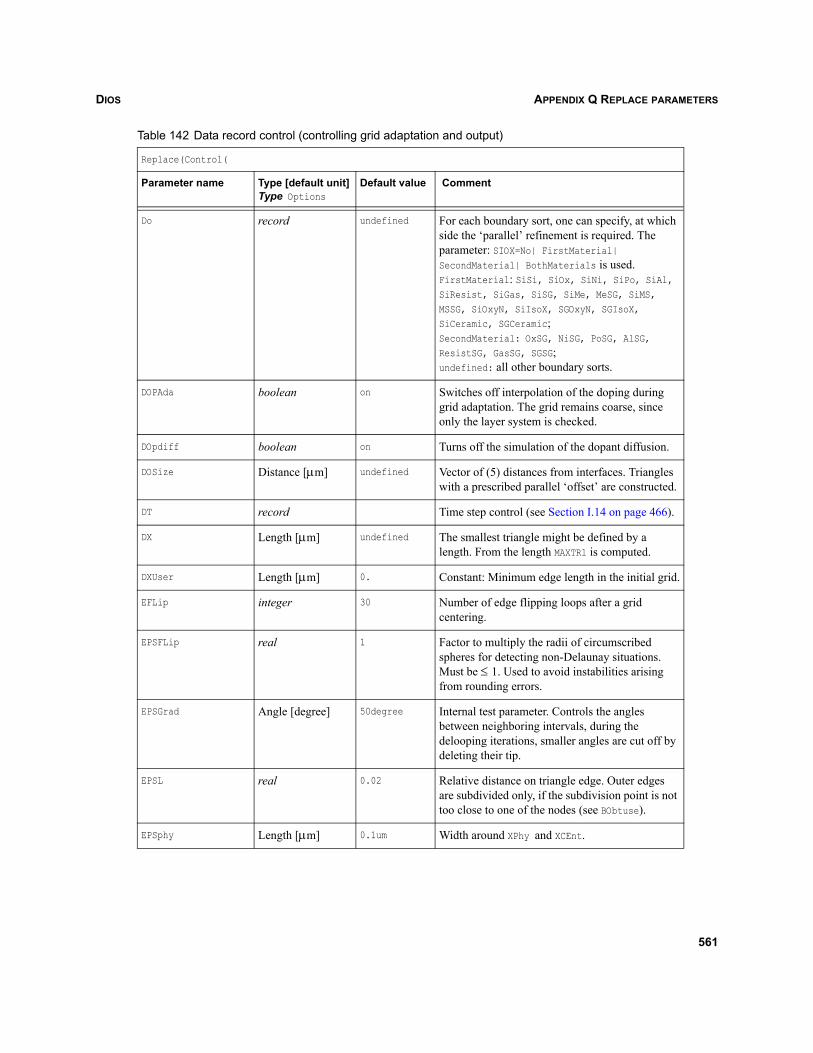
DIOS APPENDIX Q REPLACE PARAMETERS
Do record undefined For each boundary sort, one can specify, at which side the ‘parallel’ refinement is required. The parameter: SIOX=No| FirstMaterial| SecondMaterial| BothMaterials is used.FirstMaterial: SiSi, SiOx, SiNi, SiPo, SiAl, SiResist, SiGas, SiSG, SiMe, MeSG, SiMS, MSSG, SiOxyN, SiIsoX, SGOxyN, SGIsoX, SiCeramic, SGCeramic;SecondMaterial: OxSG, NiSG, PoSG, AlSG, ResistSG, GasSG, SGSG;undefined: all other boundary sorts.
DOPAda boolean on Switches off interpolation of the doping during grid adaptation. The grid remains coarse, since only the layer system is checked.
DOpdiff boolean on Turns off the simulation of the dopant diffusion.
DOSize Distance [μm] undefined Vector of (5) distances from interfaces. Triangles with a prescribed parallel ‘offset’ are constructed.
DT record Time step control (see Section I.14 on page 466).
DX Length [μm] undefined The smallest triangle might be defined by a length. From the length MAXTRl is computed.
DXUser Length [μm] 0. Constant: Minimum edge length in the initial grid.
EFLip integer 30 Number of edge flipping loops after a grid centering.
EPSFLip real 1 Factor to multiply the radii of circumscribed spheres for detecting non-Delaunay situations. Must be ≤ 1. Used to avoid instabilities arising from rounding errors.
EPSGrad Angle [degree] 50degree Internal test parameter. Controls the angles between neighboring intervals, during the delooping iterations, smaller angles are cut off by deleting their tip.
EPSL real 0.02 Relative distance on triangle edge. Outer edges are subdivided only, if the subdivision point is not too close to one of the nodes (see BObtuse).
EPSphy Length [μm] 0.1um Width around XPhy and XCEnt.
Table 142 Data record control (controlling grid adaptation and output)
Replace(Control(
Parameter name Type [default unit]Type Options
Default value Comment
561
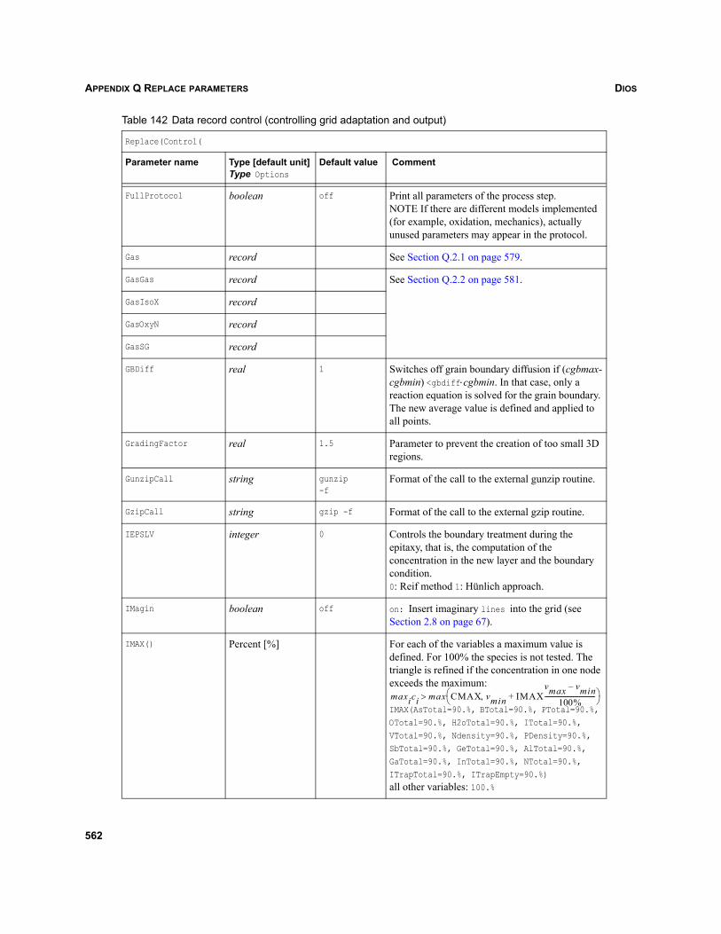
DIOSAPPENDIX Q REPLACE PARAMETERS
FullProtocol boolean off Print all parameters of the process step. NOTE If there are different models implemented (for example, oxidation, mechanics), actually unused parameters may appear in the protocol.
Gas record See Section Q.2.1 on page 579.
GasGas record See Section Q.2.2 on page 581.
GasIsoX record
GasOxyN record
GasSG record
GBDiff real 1 Switches off grain boundary diffusion if (cgbmax-cgbmin) <gbdiff⋅cgbmin. In that case, only a reaction equation is solved for the grain boundary. The new average value is defined and applied to all points.
GradingFactor real 1.5 Parameter to prevent the creation of too small 3D regions.
GunzipCall string gunzip-f
Format of the call to the external gunzip routine.
GzipCall string gzip -f Format of the call to the external gzip routine.
IEPSLV integer 0 Controls the boundary treatment during the epitaxy, that is, the computation of the concentration in the new layer and the boundary condition. 0: Reif method 1: Hünlich approach.
IMagin boolean off on: Insert imaginary lines into the grid (see Section 2.8 on page 67).
IMAX() Percent [%] For each of the variables a maximum value is defined. For 100% the species is not tested. The triangle is refined if the concentration in one node exceeds the maximum:
IMAX(AsTotal=90.%, BTotal=90.%, PTotal=90.%, OTotal=90.%, H2oTotal=90.%, ITotal=90.%, VTotal=90.%, Ndensity=90.%, PDensity=90.%, SbTotal=90.%, GeTotal=90.%, AlTotal=90.%, GaTotal=90.%, InTotal=90.%, NTotal=90.%, ITrapTotal=90.%, ITrapEmpty=90.%)all other variables: 100.%
Table 142 Data record control (controlling grid adaptation and output)
Replace(Control(
Parameter name Type [default unit]Type Options
Default value Comment
maxici max CMAX v, min IMAXvmax vmin–
100%--------------------------------+⎝ ⎠
⎛ ⎞>
562
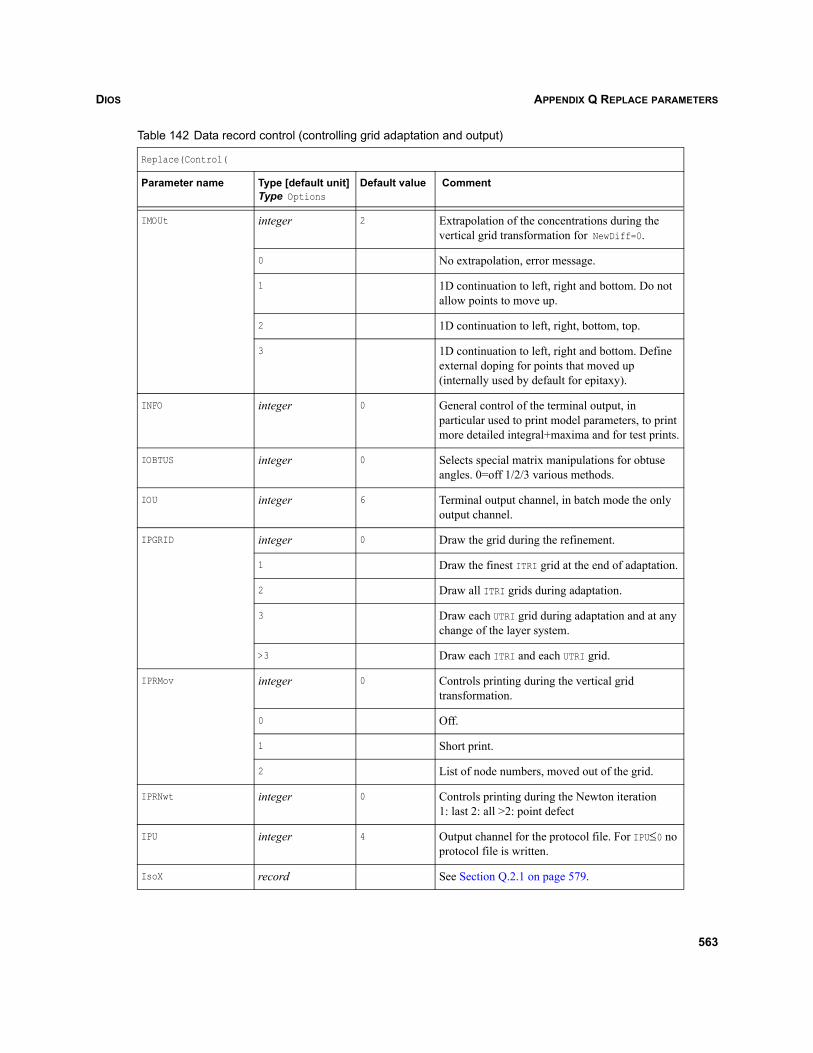
DIOS APPENDIX Q REPLACE PARAMETERS
IMOUt integer 2 Extrapolation of the concentrations during the vertical grid transformation for NewDiff=0.
0 No extrapolation, error message.
1 1D continuation to left, right and bottom. Do not allow points to move up.
2 1D continuation to left, right, bottom, top.
3 1D continuation to left, right and bottom. Define external doping for points that moved up (internally used by default for epitaxy).
INFO integer 0 General control of the terminal output, in particular used to print model parameters, to print more detailed integral+maxima and for test prints.
IOBTUS integer 0 Selects special matrix manipulations for obtuse angles. 0=off 1/2/3 various methods.
IOU integer 6 Terminal output channel, in batch mode the only output channel.
IPGRID integer 0 Draw the grid during the refinement.
1 Draw the finest ITRI grid at the end of adaptation.
2 Draw all ITRI grids during adaptation.
3 Draw each UTRI grid during adaptation and at any change of the layer system.
>3 Draw each ITRI and each UTRI grid.
IPRMov integer 0 Controls printing during the vertical grid transformation.
0 Off.
1 Short print.
2 List of node numbers, moved out of the grid.
IPRNwt integer 0 Controls printing during the Newton iteration 1: last 2: all >2: point defect
IPU integer 4 Output channel for the protocol file. For IPU≤0 no protocol file is written.
IsoX record See Section Q.2.1 on page 579.
Table 142 Data record control (controlling grid adaptation and output)
Replace(Control(
Parameter name Type [default unit]Type Options
Default value Comment
563
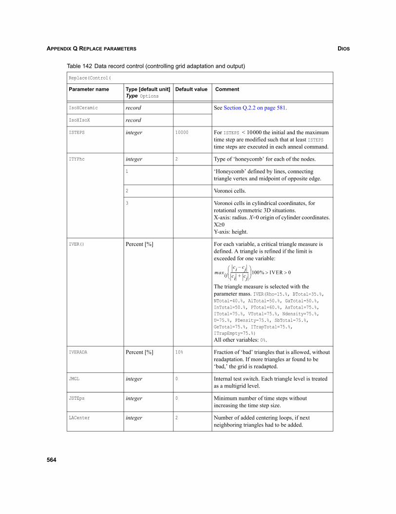
DIOSAPPENDIX Q REPLACE PARAMETERS
IsoXCeramic record See Section Q.2.2 on page 581.
IsoXIsoX record
ISTEPS integer 10000 For ISTEPS < 10000 the initial and the maximum time step are modified such that at least ISTEPS time steps are executed in each anneal command.
ITYPhc integer 2 Type of ‘honeycomb’ for each of the nodes.
1 ‘Honeycomb’ defined by lines, connecting triangle vertex and midpoint of opposite edge.
2 Voronoi cells.
3 Voronoi cells in cylindrical coordinates, for rotational symmetric 3D situations.X-axis: radius. X=0 origin of cylinder coordinates. X≥0Y-axis: height.
IVER() Percent [%] For each variable, a critical triangle measure is defined. A triangle is refined if the limit is exceeded for one variable:
The triangle measure is selected with the parameter mass. IVER(Rho=15.%, BTotal=35.%, NTotal=40.%, AlTotal=50.%, GaTotal=50.%, InTotal=50.%, PTotal=60.%, AsTotal=75.%, ITotal=75.%, VTotal=75.%, Ndensity=75.%, U=75.%, PDensity=75.%, SbTotal=75.%, GeTotal=75.%, ITrapTotal=75.%, ITrapEmpty=75.%)All other variables: 0%.
IVERADA Percent [%] 10% Fraction of ‘bad’ triangles that is allowed, without readaptation. If more triangles ar found to be ‘bad,’ the grid is readapted.
JMGL integer 0 Internal test switch. Each triangle level is treated as a multigrid level.
JSTEps integer 0 Minimum number of time steps without increasing the time step size.
LACenter integer 2 Number of added centering loops, if next neighboring triangles had to be added.
Table 142 Data record control (controlling grid adaptation and output)
Replace(Control(
Parameter name Type [default unit]Type Options
Default value Comment
maxijci cj–
ci cj+---------------------
⎝ ⎠⎜ ⎟⎛ ⎞
100% IVER 0>>
564
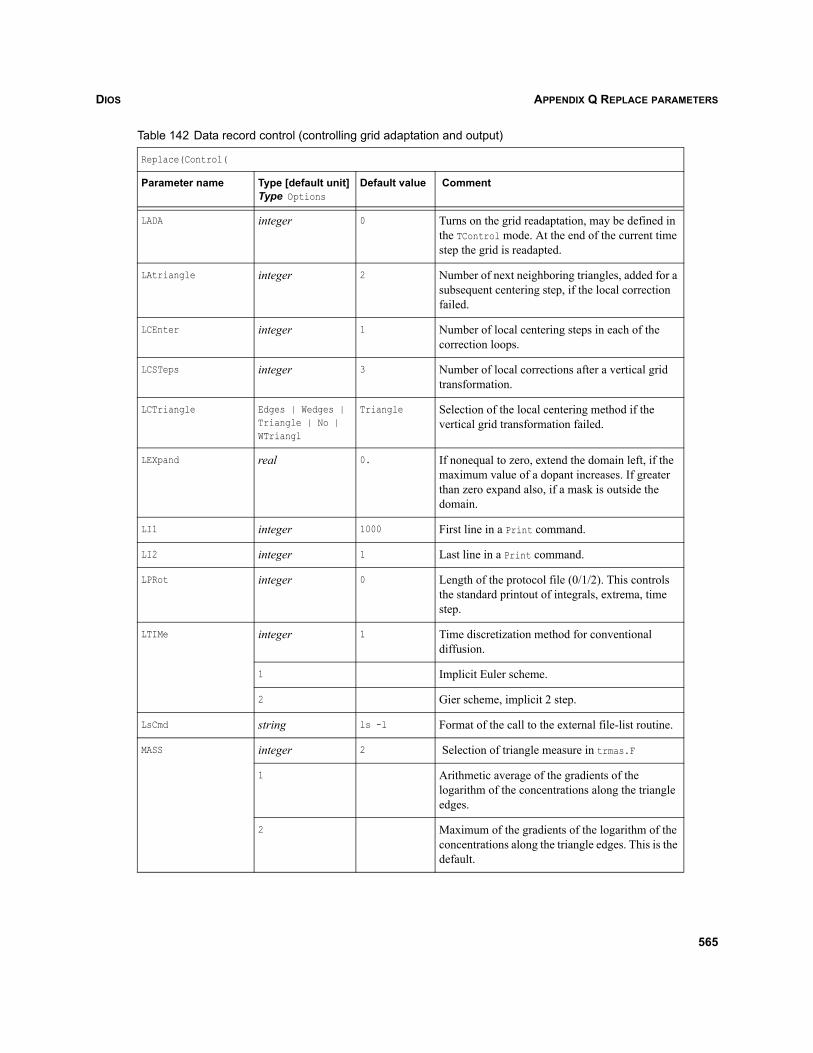
DIOS APPENDIX Q REPLACE PARAMETERS
LADA integer 0 Turns on the grid readaptation, may be defined in the TControl mode. At the end of the current time step the grid is readapted.
LAtriangle integer 2 Number of next neighboring triangles, added for a subsequent centering step, if the local correction failed.
LCEnter integer 1 Number of local centering steps in each of the correction loops.
LCSTeps integer 3 Number of local corrections after a vertical grid transformation.
LCTriangle Edges | Wedges | Triangle | No | WTriangl
Triangle Selection of the local centering method if the vertical grid transformation failed.
LEXpand real 0. If nonequal to zero, extend the domain left, if the maximum value of a dopant increases. If greater than zero expand also, if a mask is outside the domain.
LI1 integer 1000 First line in a Print command.
LI2 integer 1 Last line in a Print command.
LPRot integer 0 Length of the protocol file (0/1/2). This controls the standard printout of integrals, extrema, time step.
LTIMe integer 1 Time discretization method for conventional diffusion.
1 Implicit Euler scheme.
2 Gier scheme, implicit 2 step.
LsCmd string ls -l Format of the call to the external file-list routine.
MASS integer 2 Selection of triangle measure in trmas.F
1 Arithmetic average of the gradients of the logarithm of the concentrations along the triangle edges.
2 Maximum of the gradients of the logarithm of the concentrations along the triangle edges. This is the default.
Table 142 Data record control (controlling grid adaptation and output)
Replace(Control(
Parameter name Type [default unit]Type Options
Default value Comment
565
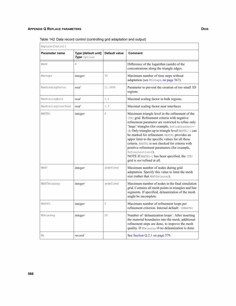
DIOSAPPENDIX Q REPLACE PARAMETERS
MASS 6 Difference of the logarithm (asinh) of the concentrations along the triangle edges.
MAsteps integer 30 Maximum number of time steps without adaptation (see MIsteps on page 567).
MaxGradingFactor real 11.3906 Parameter to prevent the creation of too small 3D regions
MaxScalingBulk real 1.1 Maximal scaling factor in bulk regions.
MaxScalingInterface real 1.3 Maximal scaling factor near interfaces
MAXTRl integer 4 Maximum triangle level in the refinement of the ITRI grid. Refinement criteria with negative refinement parameter are restricted to refine only ‘large’ triangles (for example, RefineGradient=-4). Only triangles up to triangle level MAXTRl-1 can be marked for refinement. MAXTRL provides an upper limit to the specific values for all these criteria. MAXTRL is not checked for criteria with positive refinement parameters (for example, RefineJunction=2).NOTE If MAXTRl=1 has been specified, the ITRI grid is not refined at all.
MAXV integer undefined Maximum number of nodes during grid adaptation. Specify this value to limit the mesh size (rather that MAXVDelaunay).
MAXVDelaunay integer undefined Maximum number of nodes in the final simulation grid. Contains all mesh points in triangles and line segments. If specified, delaunization of the mesh might be incomplete.
MAXVFL integer 0 Maximum number of refinement loops per refinement criterion. Internal default: 2ÞMAXTRl
MDelaunay integer 20 Number of ‘delaunization loops’. After inserting the material boundaries into the mesh, additional refinement steps are done, to improve the mesh quality. If MDelaunay=0 no delaunization is done.
Me record See Section Q.2.1 on page 579.
Table 142 Data record control (controlling grid adaptation and output)
Replace(Control(
Parameter name Type [default unit]Type Options
Default value Comment
566
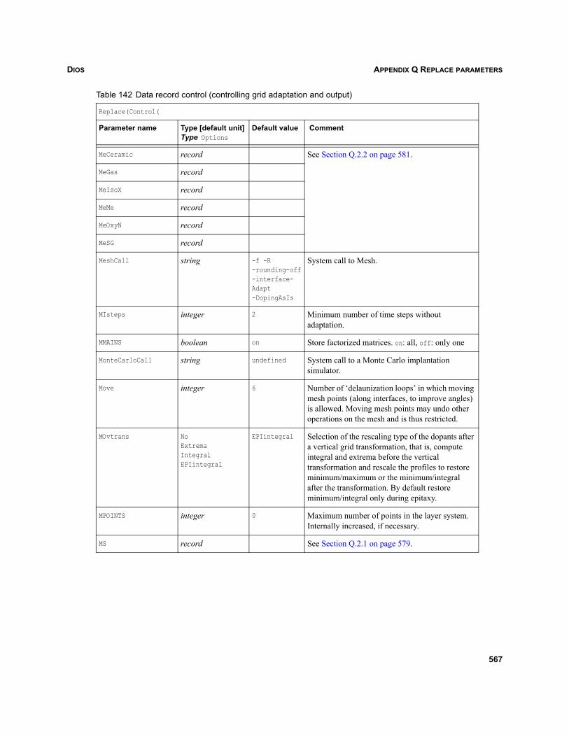
DIOS APPENDIX Q REPLACE PARAMETERS
MeCeramic record See Section Q.2.2 on page 581.
MeGas record
MeIsoX record
MeMe record
MeOxyN record
MeSG record
MeshCall string -f -R-rounding-off-interface-Adapt-DopingAsIs
System call to Mesh.
MIsteps integer 2 Minimum number of time steps without adaptation.
MMAINS boolean on Store factorized matrices. on: all, off: only one
MonteCarloCall string undefined System call to a Monte Carlo implantation simulator.
Move integer 6 Number of ‘delaunization loops’ in which moving mesh points (along interfaces, to improve angles) is allowed. Moving mesh points may undo other operations on the mesh and is thus restricted.
MOvtrans NoExtremaIntegralEPIintegral
EPIintegral Selection of the rescaling type of the dopants after a vertical grid transformation, that is, compute integral and extrema before the vertical transformation and rescale the profiles to restore minimum/maximum or the minimum/integral after the transformation. By default restore minimum/integral only during epitaxy.
MPOINTS integer 0 Maximum number of points in the layer system. Internally increased, if necessary.
MS record See Section Q.2.1 on page 579.
Table 142 Data record control (controlling grid adaptation and output)
Replace(Control(
Parameter name Type [default unit]Type Options
Default value Comment
567
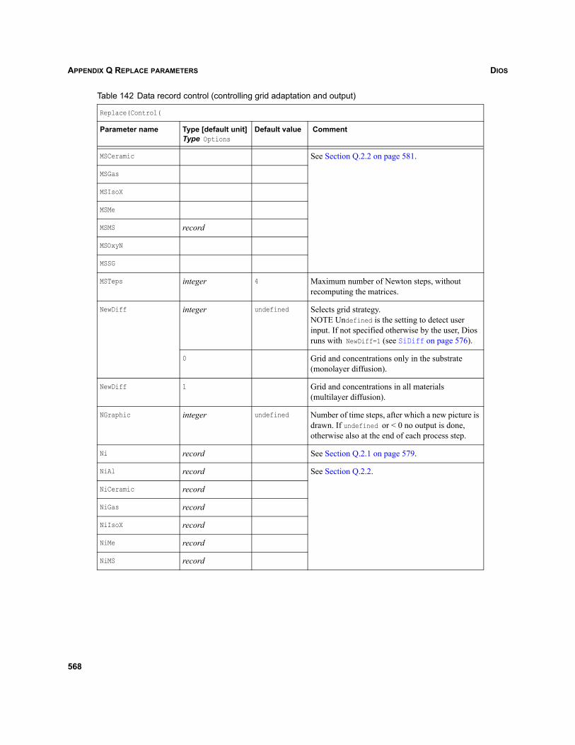
DIOSAPPENDIX Q REPLACE PARAMETERS
MSCeramic See Section Q.2.2 on page 581.
MSGas
MSIsoX
MSMe
MSMS record
MSOxyN
MSSG
MSTeps integer 4 Maximum number of Newton steps, without recomputing the matrices.
NewDiff integer undefined Selects grid strategy. NOTE Undefined is the setting to detect user input. If not specified otherwise by the user, Dios runs with NewDiff=1 (see SiDiff on page 576).
0 Grid and concentrations only in the substrate (monolayer diffusion).
NewDiff 1 Grid and concentrations in all materials (multilayer diffusion).
NGraphic integer undefined Number of time steps, after which a new picture is drawn. If undefined or < 0 no output is done, otherwise also at the end of each process step.
Ni record See Section Q.2.1 on page 579.
NiAl record See Section Q.2.2.
NiCeramic record
NiGas record
NiIsoX record
NiMe record
NiMS record
Table 142 Data record control (controlling grid adaptation and output)
Replace(Control(
Parameter name Type [default unit]Type Options
Default value Comment
568
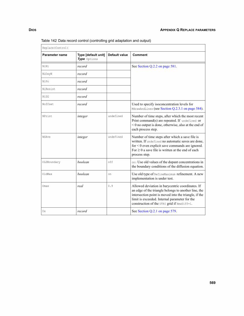
DIOS APPENDIX Q REPLACE PARAMETERS
NiNi record See Section Q.2.2 on page 581.
NiOxyN record
NiPo record
NiResist record
NiSG record
Noffset record Used to specify isoconcentration levels for MdrawAndLines (see Section Q.2.3.1 on page 584).
NPrint integer undefined Number of time steps, after which the most recent Print command(s) are repeated. If undefined or < 0 no output is done, otherwise, also at the end of each process step.
NSAve integer undefined Number of time steps after which a save file is written. If undefined no automatic saves are done, for < 0 even explicit save commands are ignored. For ≥ 0 a save file is written at the end of each process step.
OLDBoundary boolean off on: Use old values of the dopant concentrations in the boundary conditions of the diffusion equation.
OldMax boolean on Use old type of RefineMaximum refinement. A new implementation is under test.
Omax real 0.9 Allowed deviation in barycentric coordinates. If an edge of the triangle belongs to another line, the intersection point is moved into the triangle, if the limit is exceeded. Internal parameter for the construction of the UTRI grid if NewDiff=1.
Ox record See Section Q.2.1 on page 579.
Table 142 Data record control (controlling grid adaptation and output)
Replace(Control(
Parameter name Type [default unit]Type Options
Default value Comment
569
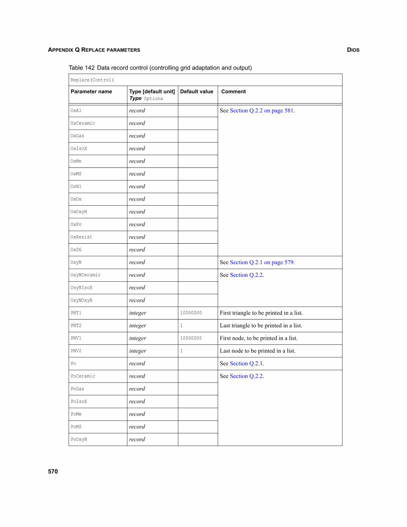
DIOSAPPENDIX Q REPLACE PARAMETERS
OxAl record See Section Q.2.2 on page 581.
OxCeramic record
OxGas record
OxIsoX record
OxMe record
OxMS record
OxNi record
OxOx record
OxOxyN record
OxPo record
OxResist record
OxSG record
OxyN record See Section Q.2.1 on page 579.
OxyNCeramic record See Section Q.2.2.
OxyNIsoX record
OxyNOxyN record
PNT1 integer 10000000 First triangle to be printed in a list.
PNT2 integer 1 Last triangle to be printed in a list.
PNV1 integer 10000000 First node, to be printed in a list.
PNV2 integer 1 Last node to be printed in a list.
Po record See Section Q.2.1.
PoCeramic record See Section Q.2.2.
PoGas record
PoIsoX record
PoMe record
PoMS record
PoOxyN record
Table 142 Data record control (controlling grid adaptation and output)
Replace(Control(
Parameter name Type [default unit]Type Options
Default value Comment
570
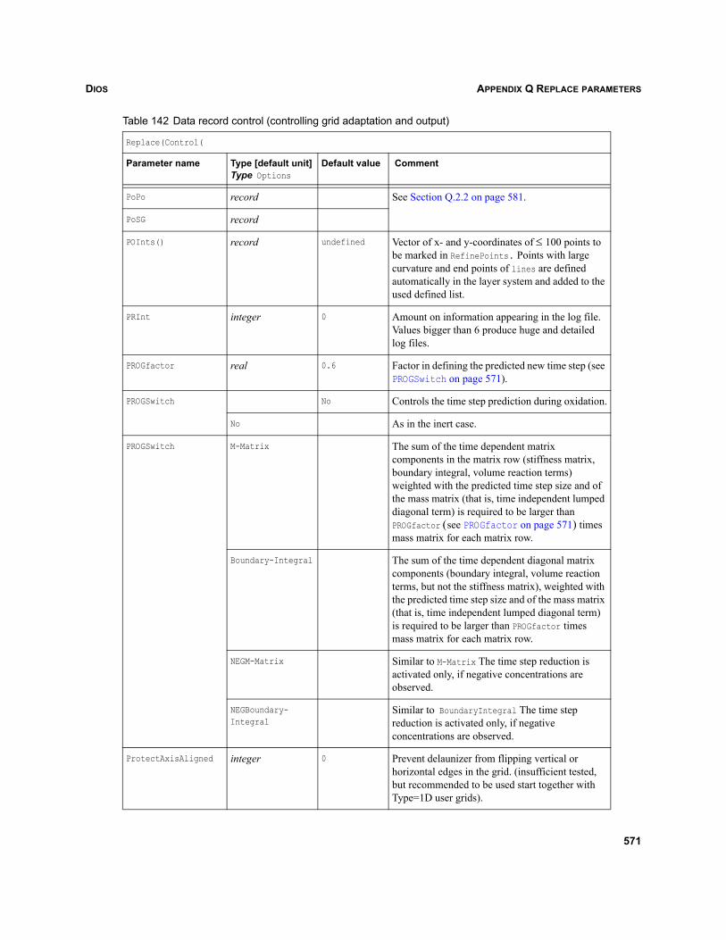
DIOS APPENDIX Q REPLACE PARAMETERS
PoPo record See Section Q.2.2 on page 581.
PoSG record
POInts() record undefined Vector of x- and y-coordinates of ≤ 100 points to be marked in RefinePoints. Points with large curvature and end points of lines are defined automatically in the layer system and added to the used defined list.
PRInt integer 0 Amount on information appearing in the log file. Values bigger than 6 produce huge and detailed log files.
PROGfactor real 0.6 Factor in defining the predicted new time step (see PROGSwitch on page 571).
PROGSwitch No Controls the time step prediction during oxidation.
No As in the inert case.
PROGSwitch M-Matrix The sum of the time dependent matrix components in the matrix row (stiffness matrix, boundary integral, volume reaction terms) weighted with the predicted time step size and of the mass matrix (that is, time independent lumped diagonal term) is required to be larger than PROGfactor (see PROGfactor on page 571) times mass matrix for each matrix row.
Boundary-Integral The sum of the time dependent diagonal matrix components (boundary integral, volume reaction terms, but not the stiffness matrix), weighted with the predicted time step size and of the mass matrix (that is, time independent lumped diagonal term) is required to be larger than PROGfactor times mass matrix for each matrix row.
NEGM-Matrix Similar to M-Matrix The time step reduction is activated only, if negative concentrations are observed.
NEGBoundary-Integral
Similar to BoundaryIntegral The time step reduction is activated only, if negative concentrations are observed.
ProtectAxisAligned integer 0 Prevent delaunizer from flipping vertical or horizontal edges in the grid. (insufficient tested, but recommended to be used start together with Type=1D user grids).
Table 142 Data record control (controlling grid adaptation and output)
Replace(Control(
Parameter name Type [default unit]Type Options
Default value Comment
571
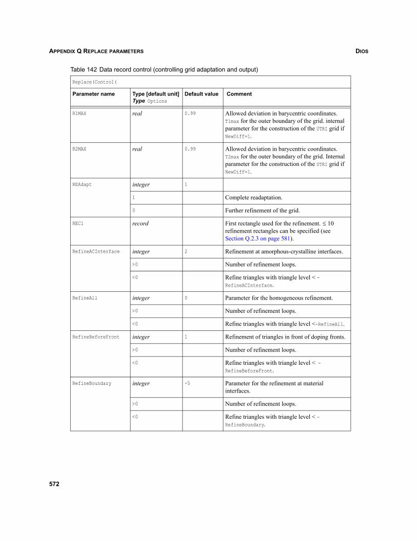
DIOSAPPENDIX Q REPLACE PARAMETERS
R1MAX real 0.99 Allowed deviation in barycentric coordinates. T1max for the outer boundary of the grid. internal parameter for the construction of the UTRI grid if NewDiff=1.
R2MAX real 0.99 Allowed deviation in barycentric coordinates. T2max for the outer boundary of the grid. Internal parameter for the construction of the UTRI grid if NewDiff=1.
REAdapt integer 1
1 Complete readaptation.
0 Further refinement of the grid.
REC1 record First rectangle used for the refinement. refinement rectangles can be specified (see Section Q.2.3 on page 581).
RefineACInterface integer 2 Refinement at amorphous-crystalline interfaces.
>0 Number of refinement loops.
<0 Refine triangles with triangle level < -RefineACInterface.
RefineAll integer 0 Parameter for the homogeneous refinement.
>0 Number of refinement loops.
<0 Refine triangles with triangle level <-RefineAll.
RefineBeforeFront integer 1 Refinement of triangles in front of doping fronts.
>0 Number of refinement loops.
<0 Refine triangles with triangle level < -RefineBeforeFront.
RefineBoundary integer -5 Parameter for the refinement at material interfaces.
>0 Number of refinement loops.
<0 Refine triangles with triangle level < -RefineBoundary.
Table 142 Data record control (controlling grid adaptation and output)
Replace(Control(
Parameter name Type [default unit]Type Options
Default value Comment
10≤
572
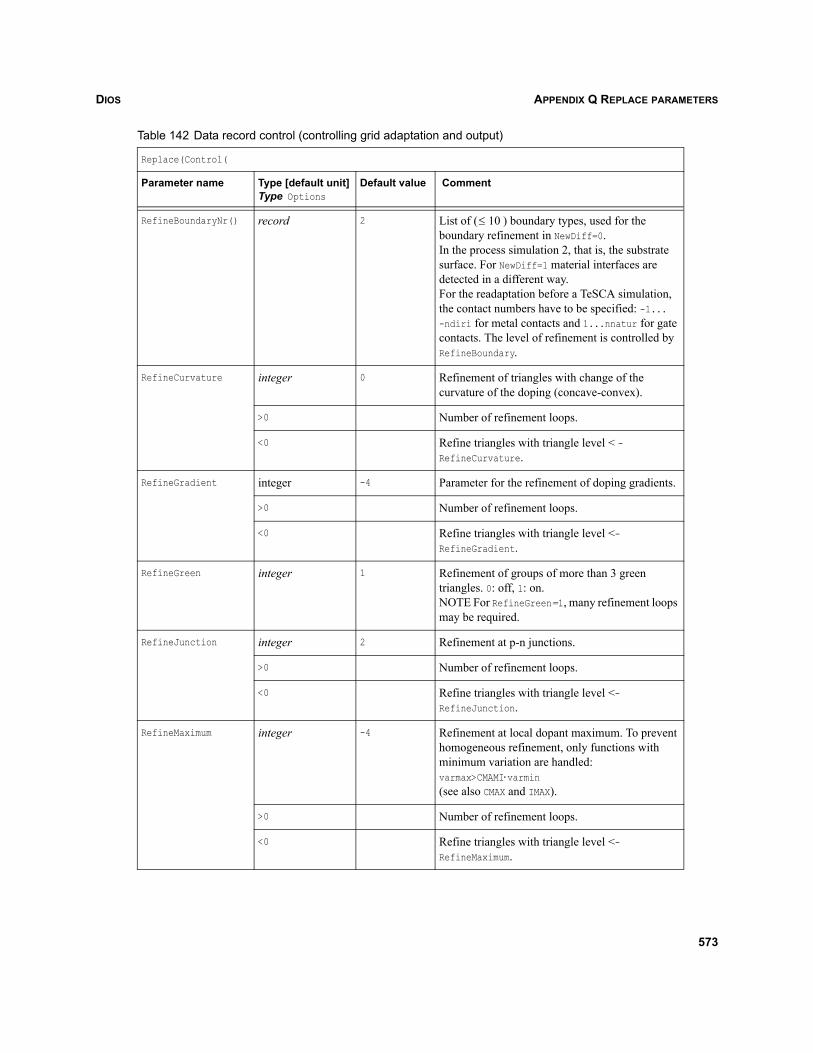
DIOS APPENDIX Q REPLACE PARAMETERS
RefineBoundaryNr() record 2 List of ( ) boundary types, used for the boundary refinement in NewDiff=0.In the process simulation 2, that is, the substrate surface. For NewDiff=1 material interfaces are detected in a different way. For the readaptation before a TeSCA simulation, the contact numbers have to be specified: -1...-ndiri for metal contacts and 1...nnatur for gate contacts. The level of refinement is controlled by RefineBoundary.
RefineCurvature integer 0 Refinement of triangles with change of the curvature of the doping (concave-convex).
>0 Number of refinement loops.
<0 Refine triangles with triangle level < -RefineCurvature.
RefineGradient integer -4 Parameter for the refinement of doping gradients.
>0 Number of refinement loops.
<0 Refine triangles with triangle level <-RefineGradient.
RefineGreen integer 1 Refinement of groups of more than 3 green triangles. 0: off, 1: on. NOTE For RefineGreen=1, many refinement loops may be required.
RefineJunction integer 2 Refinement at p-n junctions.
>0 Number of refinement loops.
<0 Refine triangles with triangle level <-RefineJunction.
RefineMaximum integer -4 Refinement at local dopant maximum. To prevent homogeneous refinement, only functions with minimum variation are handled: varmax>CMAMI⋅varmin(see also CMAX and IMAX).
>0 Number of refinement loops.
<0 Refine triangles with triangle level <-RefineMaximum.
Table 142 Data record control (controlling grid adaptation and output)
Replace(Control(
Parameter name Type [default unit]Type Options
Default value Comment
10≤
573
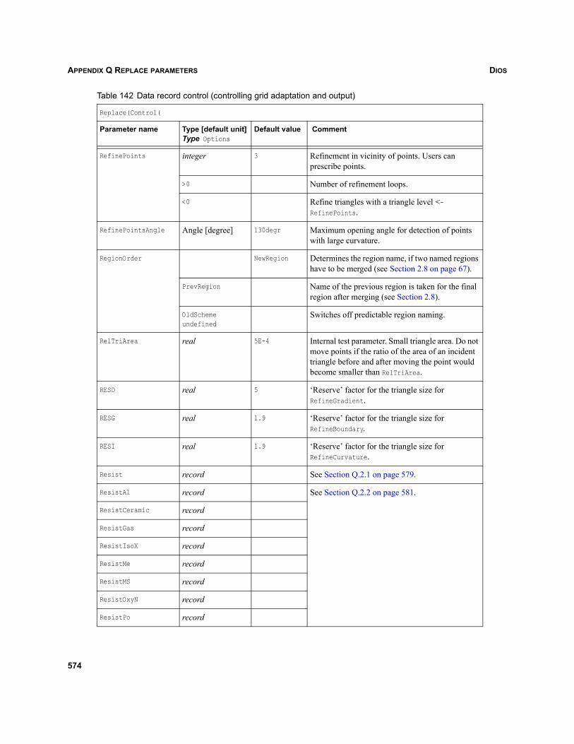
DIOSAPPENDIX Q REPLACE PARAMETERS
RefinePoints integer 3 Refinement in vicinity of points. Users can prescribe points.
>0 Number of refinement loops.
<0 Refine triangles with a triangle level <-RefinePoints.
RefinePointsAngle Angle [degree] 130degr Maximum opening angle for detection of points with large curvature.
RegionOrder NewRegion Determines the region name, if two named regions have to be merged (see Section 2.8 on page 67).
PrevRegion Name of the previous region is taken for the final region after merging (see Section 2.8).
OldSchemeundefined
Switches off predictable region naming.
RelTriArea real 5E-4 Internal test parameter. Small triangle area. Do not move points if the ratio of the area of an incident triangle before and after moving the point would become smaller than RelTriArea.
RESD real 5 ‘Reserve’ factor for the triangle size for RefineGradient.
RESG real 1.9 ‘Reserve’ factor for the triangle size for RefineBoundary.
RESI real 1.9 ‘Reserve’ factor for the triangle size for RefineCurvature.
Resist record See Section Q.2.1 on page 579.
ResistAl record See Section Q.2.2 on page 581.
ResistCeramic record
ResistGas record
ResistIsoX record
ResistMe record
ResistMS record
ResistOxyN record
ResistPo record
Table 142 Data record control (controlling grid adaptation and output)
Replace(Control(
Parameter name Type [default unit]Type Options
Default value Comment
574
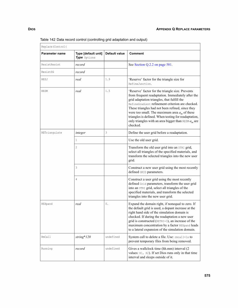
DIOS APPENDIX Q REPLACE PARAMETERS
ResistResist record See Section Q.2.2 on page 581.
ResistSG record
RESJ real 1.9 ‘Reserve’ factor for the triangle size for RefineJunction.
RESM real 1.5 ‘Reserve’ factor for the triangle size. Prevents from frequent readaptation. Immediately after the grid adaptation triangles, that fulfill the RefineGradient refinement criterion are checked. These triangles had not been refined, since they were too small. The maximum area am of these triangles is defined. When testing for readaptation, only triangles with an area bigger than RESM⋅am are checked.
RETriangulate integer 3 Define the user grid before a readaptation.
1 Use the old user grid.
2 Transform the old user grid into an UTRI grid, select all triangles of the specified materials, and transform the selected triangles into the new user grid.
3 Construct a new user grid using the most recently defined GRID parameters.
4 Construct a user grid using the most recently defined Grid parameters, transform the user grid into an UTRI grid, select all triangles of the specified materials, and transform the selected triangles into the new user grid.
REXpand real 0. Expand the domain right, if nonequal to zero. If the default grid is used, a dopant increase at the right hand side of the simulation domain is checked. If during the readaptation a new user grid is constructed (RETRI=3), an increase of the maximum concentration by a factor REXpand leads to a lateral expansion of the simulation domain.
RmCall string*120 undefined System call to delete a file. Use: rmcall=ls to prevent temporary files from being removed.
Running record undefined Gives a wallclock time (hh.mm) interval (2 values: R1, R2). If set Dios runs only in that time interval and sleeps outside of it.
Table 142 Data record control (controlling grid adaptation and output)
Replace(Control(
Parameter name Type [default unit]Type Options
Default value Comment
575
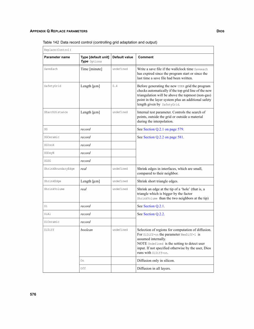
DIOSAPPENDIX Q REPLACE PARAMETERS
SaveEach Time [minute] undefined Write a save file if the wallclock time Saveeach has expired since the program start or since the last time a save file had been written.
SafetyGrid Length [μm] 0.4 Before generating the new USER grid the program checks automatically if the top grid line of the new triangulation will be above the topmost (non-gas) point in the layer system plus an additional safety length given by SafetyGrid.
SEarchDistance Length [μm] undefined Internal test parameter. Controls the search of points, outside the grid or outside a material during the interpolation.
SG record See Section Q.2.1 on page 579.
SGCeramic record See Section Q.2.2 on page 581.
SGIsoX record
SGOxyN record
SGSG record
ShrinkBoundaryEdge real undefined Shrink edges in interfaces, which are small, compared to their neighbor.
ShrinkEdge Length [μm] undefined Shrink short triangle edges.
ShrinkVolume real undefined Shrink an edge at the tip of a ‘hole’ (that is, a triangle which is bigger by the factor ShrinkVolume than the two neighbors at the tip)
Si record See Section Q.2.1.
SiAl record See Section Q.2.2.
SiCeramic record
SiDiff boolean undefined Selection of regions for computation of diffusion. For SiDiff=on the parameter NewDiff=1 is assumed internally.NOTE Undefined is the setting to detect user input. If not specified otherwise by the user, Dios runs with SiDiff=on.
On Diffusion only in silicon.
Off Diffusion in all layers.
Table 142 Data record control (controlling grid adaptation and output)
Replace(Control(
Parameter name Type [default unit]Type Options
Default value Comment
576
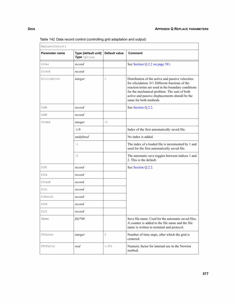
DIOS APPENDIX Q REPLACE PARAMETERS
SiGas record See Section Q.2.2 on page 581.
SiIsoX record
Silicidation integer 1 Distribution of the active and passive velocities for silicidation. 0/1 Different fractions of the reaction terms are used in the boundary conditions for the mechanical problem. The sum of both active and passive displacements should be the same for both methods.
SiMe record See Section Q.2.2.
SiMS record
SIndex integer -2
Index of the first automatically saved file.
undefined No index is added.
–1 The index of a loaded file is incremented by 1 and used for the first automatically saved file.
–2 The automatic save toggles between indices 1 and 2. This is the default.
SiNi record See Section Q.2.2.
SiOx record
SiOxyN record
SiPo record
SiResist record
SiSG record
SiSi record
SName file*80 Save file name. Used for the automatic saved files. A counter is added to the file name and the file name is written to terminal and protocol.
STCenter integer 5 Number of time steps, after which the grid is centered.
STCFactor real 1.001 Numeric factor for internal use in the Newton method.
Table 142 Data record control (controlling grid adaptation and output)
Replace(Control(
Parameter name Type [default unit]Type Options
Default value Comment
0≥
577
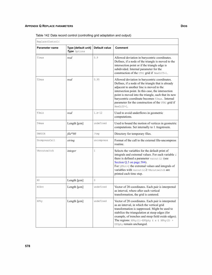
DIOSAPPENDIX Q REPLACE PARAMETERS
T1max real 0.9 Allowed deviation in barycentric coordinates. Defines, if a node of the triangle is moved to the intersection point or if the triangle edge is subdivided. Internal parameter for the construction of the UTRI grid if NewDiff=1.
T2max real 0.95 Allowed deviation in barycentric coordinates. Defines, if a node of the triangle that is already adjacent to another line is moved to the intersection point. In this case, the intersection point is moved into the triangle, such that its new barycentric coordinate becomes T2max. Internal parameter for the construction of the UTRI grid if NewDiff=1.
T3min real 1.e-12 Used to avoid underflows in geometric computations.
T4max Length [μm] undefined Used to bound the motion of vertices in geometric computations. Set internally to 1 Angstroem.
TMPDIR file*80 /tmp Directory for temporary files.
UnompressCall string uncompress Format of the call to the external file-uncompress routine.
VAroutswitch integer 1 Selects the variables for the default print of integrals and extremal values. For each variable i there is defined a parameter varout(i) (see Section Q.3 on page 584).For LPRot=2 the extremal values and integrals of variables with varout(i)≥ VAroutswitch are printed each time step.
X0 Length [μm] 0
XCEnt Length [μm] undefined Vector of 20 coordinates. Each pair is interpreted as interval, where after each vertical transformation, the grid is centered.
XPhy Length [μm] undefined Vector of 20 coordinates. Each pair is interpreted as an interval, in which the vertical grid transformation is suppressed. Might be used to stabilize the triangulation at steep edges (for example, of trenches and steep field oxide edges). The regions: XPhy(1)-EPSphy £ x £ XPhy(2) + EPSphy remain unchanged.
Table 142 Data record control (controlling grid adaptation and output)
Replace(Control(
Parameter name Type [default unit]Type Options
Default value Comment
578
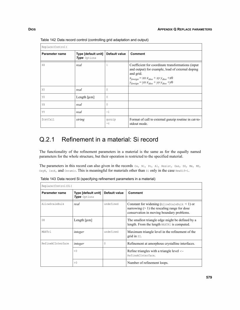
DIOS APPENDIX Q REPLACE PARAMETERS
Q.2.1 Refinement in a material: Si record
The functionality of the refinement parameters in a material is the same as for the equally namedparameters for the whole structure, but their operation is restricted to the specified material.
The parameters in this record can also given in the records Ox, Ni, Po, Al, Resist, Gas, SG, Me, MS,OxyN, IsoX, and Ceramic. This is meaningful for materials other than Si only in the case NewDif=1.
XX real 1 Coefficient for coordinate transformations (input and output) for example, load of external doping and grid.xforeign = xx⋅xdios + xy⋅ydios +x0yforeign = yx⋅xdios + yy⋅ydios +y0
XY real 0
Y0 Length [μm] 0
YX real 0
YY real -1
ZcatCall string gunzip-c
Format of call to external gunzip routine in cat-to-stdout mode.
Table 143 Data record Si (specifying refinement parameters in a material)
Replace(Control(Si(
Parameter name Type [default unit]Type Options
Default value Comment
AllowScaleBulk real undefined Constant for widening (AllowScaleBulk < 1) or narrowing (> 1) the rescaling range for dose conservation in moving boundary problems.
DX Length [μm] The smallest triangle edge might be defined by a length. From the length MAXTRl is computed.
MAXTrl integer undefined Maximum triangle level in the refinement of the grid in SI.
RefineACInterface integer 0 Refinement at amorphous crystalline interfaces.
<0 Refine triangles with a triangle level <-RefineACInterface.
>0 Number of refinement loops.
Table 142 Data record control (controlling grid adaptation and output)
Replace(Control(
Parameter name Type [default unit]Type Options
Default value Comment
579
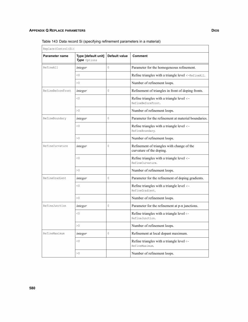
DIOSAPPENDIX Q REPLACE PARAMETERS
RefineAll integer 0 Parameter for the homogeneous refinement.
<0 Refine triangles with a triangle level <-RefineAll.
>0 Number of refinement loops.
RefineBeforeFront integer 0 Refinement of triangles in front of doping fronts.
<0 Refine triangles with a triangle level <-RefineBeforeFront.
>0 Number of refinement loops.
RefineBoundary integer 0 Parameter for the refinement at material boundaries.
<0 Refine triangles with a triangle level <-RefineBoundary.
>0 Number of refinement loops.
RefineCurvature integer 0 Refinement of triangles with change of the curvature of the doping.
<0 Refine triangles with a triangle level <-RefineCurvature.
>0 Number of refinement loops.
RefineGradient integer 0 Parameter for the refinement of doping gradients.
<0 Refine triangles with a triangle level <-RefineGradient.
>0 Number of refinement loops.
RefineJunction integer 0 Parameter for the refinement at p-n junctions.
<0 Refine triangles with a triangle level <-RefineJunction.
>0 Number of refinement loops.
RefineMaximum integer 0 Refinement at local dopant maximum.
<0 Refine triangles with a triangle level <-RefineMaximum.
>0 Number of refinement loops.
Table 143 Data record Si (specifying refinement parameters in a material)
Replace(Control(Si(
Parameter name Type [default unit]Type Options
Default value Comment
580
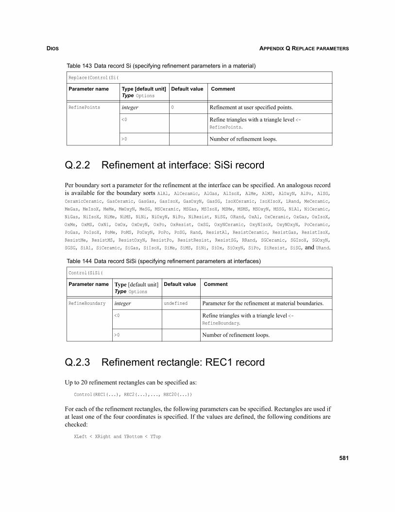
DIOS APPENDIX Q REPLACE PARAMETERS
Q.2.2 Refinement at interface: SiSi record
Per boundary sort a parameter for the refinement at the interface can be specified. An analogous recordis available for the boundary sorts AlAl, AlCeramic, AlGas, AlIsoX, AlMe, AlMS, AlOxyN, AlPo, AlSG,CeramicCeramic, GasCeramic, GasGas, GasIsoX, GasOxyN, GasSG, IsoXCeramic, IsoXIsoX, LRand, MeCeramic,
MeGas, MeIsoX, MeMe, MeOxyN, MeSG, MSCeramic, MSGas, MSIsoX, MSMe, MSMS, MSOxyN, MSSG, NiAl, NiCeramic,
NiGas, NiIsoX, NiMe, NiMS, NiNi, NiOxyN, NiPo, NiResist, NiSG, ORand, OxAl, OxCeramic, OxGas, OxIsoX,
OxMe, OxMS, OxNi, OxOx, OxOxyN, OxPo, OxResist, OxSG, OxyNCeramic, OxyNIsoX, OxyNOxyN, PoCeramic,
PoGas, PoIsoX, PoMe, PoMS, PoOxyN, PoPo, PoSG, Rand, ResistAl, ResistCeramic, ResistGas, ResistIsoX,
ResistMe, ResistMS, ResistOxyN, ResistPo, ResistResist, ResistSG, RRand, SGCeramic, SGIsoX, SGOxyN,
SGSG, SiAl, SiCeramic, SiGas, SiIsoX, SiMe, SiMS, SiNi, SiOx, SiOxyN, SiPo, SiResist, SiSG, and URand.
Q.2.3 Refinement rectangle: REC1 record
Up to 20 refinement rectangles can be specified as:
Control(REC1(...), REC2(...),..., REC20(...))
For each of the refinement rectangles, the following parameters can be specified. Rectangles are used ifat least one of the four coordinates is specified. If the values are defined, the following conditions arechecked:
XLeft < XRight and YBottom < YTop
RefinePoints integer 0 Refinement at user specified points.
<0 Refine triangles with a triangle level <-RefinePoints.
>0 Number of refinement loops.
Table 144 Data record SiSi (specifying refinement parameters at interfaces)
Control(SiSi(
Parameter name Type [default unit]Type Options
Default value Comment
RefineBoundary integer undefined Parameter for the refinement at material boundaries.
<0 Refine triangles with a triangle level <-RefineBoundary.
>0 Number of refinement loops.
Table 143 Data record Si (specifying refinement parameters in a material)
Replace(Control(Si(
Parameter name Type [default unit]Type Options
Default value Comment
581
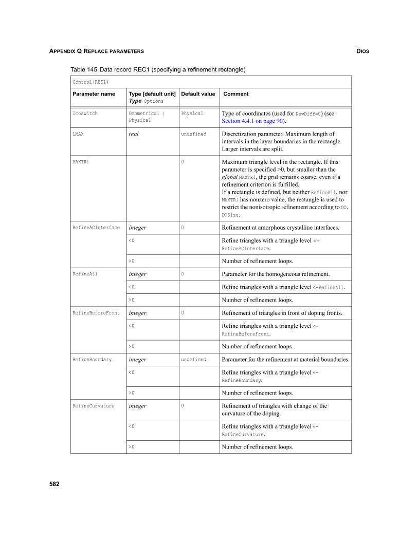
DIOSAPPENDIX Q REPLACE PARAMETERS
Table 145 Data record REC1 (specifying a refinement rectangle)
Control(REC1(
Parameter name Type [default unit]Type Options
Default value Comment
Icoswitch Geometrical | Physical
Physical Type of coordinates (used for NewDiff=0) (see Section 4.4.1 on page 90).
LMAX real undefined Discretization parameter. Maximum length of intervals in the layer boundaries in the rectangle. Larger intervals are split.
MAXTRl 0 Maximum triangle level in the rectangle. If this parameter is specified >0, but smaller than the global MAXTRl, the grid remains coarse, even if a refinement criterion is fulfilled.If a rectangle is defined, but neither RefineAll, nor MAXTRl has nonzero value, the rectangle is used to restrict the nonisotropic refinement according to DO, DOSize.
RefineACInterface integer 0 Refinement at amorphous crystalline interfaces.
<0 Refine triangles with a triangle level <-RefineACInterface.
>0 Number of refinement loops.
RefineAll integer 0 Parameter for the homogeneous refinement.
<0 Refine triangles with a triangle level <-RefineAll.
>0 Number of refinement loops.
RefineBeforeFront integer 0 Refinement of triangles in front of doping fronts.
<0 Refine triangles with a triangle level <-RefineBeforeFront.
>0 Number of refinement loops.
RefineBoundary integer undefined Parameter for the refinement at material boundaries.
<0 Refine triangles with a triangle level <-RefineBoundary.
>0 Number of refinement loops.
RefineCurvature integer 0 Refinement of triangles with change of the curvature of the doping.
<0 Refine triangles with a triangle level <-RefineCurvature.
>0 Number of refinement loops.
582
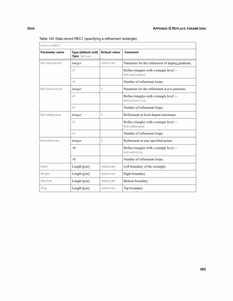
DIOS APPENDIX Q REPLACE PARAMETERS
RefineGradient integer undefined Parameter for the refinement of doping gradients.
<0 Refine triangles with a triangle level <-RefineGradient.
>0 Number of refinement loops.
RefineJunction integer 0 Parameter for the refinement at p-n junctions.
<0 Refine triangles with a triangle level <-RefineJunction.
>0 Number of refinement loops.
RefineMaximum integer 0 Refinement at local dopant maximum.
<0 Refine triangles with a triangle level <-RefineMaximum.
>0 Number of refinement loops.
RefinePoints integer 0 Refinement at user specified points.
<0 Refine triangles with a triangle level <-RefinePoints.
>0 Number of refinement loops.
XLeft Length [μm] undefined Left boundary of the rectangle.
XRight Length [μm] undefined Right boundary.
YBottom Length [μm] undefined Bottom boundary.
YTop Length [μm] undefined Top boundary.
Table 145 Data record REC1 (specifying a refinement rectangle)
Control(REC1(
Parameter name Type [default unit]Type Options
Default value Comment
583
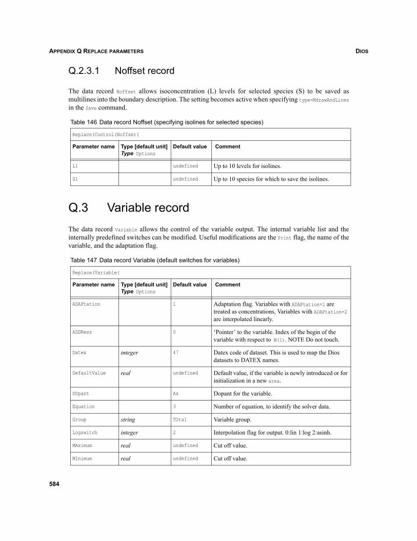
DIOSAPPENDIX Q REPLACE PARAMETERS
Q.2.3.1 Noffset record
The data record Noffset allows isoconcentration (L) levels for selected species (S) to be saved asmultilines into the boundary description. The setting becomes active when specifying type=MdrawAndLinesin the Save command.
Q.3 Variable recordThe data record Variable allows the control of the variable output. The internal variable list and theinternally predefined switches can be modified. Useful modifications are the Print flag, the name of thevariable, and the adaptation flag.
Table 146 Data record Noffset (specifying isolines for selected species)
Replace(Control(Noffset(
Parameter name Type [default unit]Type Options
Default value Comment
L1 undefined Up to 10 levels for isolines.
S1 undefined Up to 10 species for which to save the isolines.
Table 147 Data record Variable (default switches for variables)
Replace(Variable(
Parameter name Type [default unit]Type Options
Default value Comment
ADAPtation 1 Adaptation flag. Variables with ADAPtation=1 are treated as concentrations, Variables with ADAPtation=2 are interpolated linearly.
ADDRess 0 ‘Pointer’ to the variable. Index of the begin of the variable with respect to W(1). NOTE Do not touch.
Datex integer 47 Datex code of dataset. This is used to map the Dios datasets to DATEX names.
DefaultValue real undefined Default value, if the variable is newly introduced or for initialization in a new area.
DOpant As Dopant for the variable.
Equation 3 Number of equation, to identify the solver data.
Group string TOtal Variable group.
Logswitch integer 2 Interpolation flag for output. 0:lin 1:log 2:asinh.
MAximum real undefined Cut off value.
MInimum real undefined Cut off value.
584
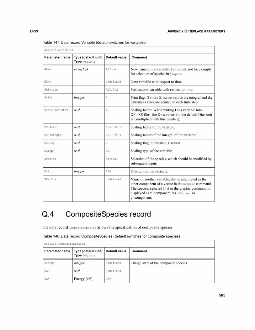
DIOS APPENDIX Q REPLACE PARAMETERS
Q.4 CompositeSpecies recordThe data record CompositeSpecies allows the specification of composite species.
NAme string*24 AsTotal New name of the variable. For output, not for example, for selection of species in graphic.
NExt undefined Next variable with respect to time.
PREvious AsToOld Predecessor variable with respect to time.
Print integer 2 Print flag. If PRInt ≥ VAroutswitch the integral and the extremal values are printed in each time step.
ScaleDiosDatex real 1. Scaling factor. When writing Dios variable into DF–ISE files, the Dios values (in the default Dios unit are multiplied with this number).
SCFActor real 6.43045E17 Scaling factor of the variable.
SCFIntegral real 6.43045E9 Scaling factor of the integral of the variable.
SCFLag real 0 Scaling flag 0:unscaled, 1:scaled.
SCType real 2NI Scaling type of the variable.
SPecies AsTotal Selection of the species, which should be modified by subsequent input.
Unit integer 196 Dios unit of the variable.
VPartner undefined Name of another variable, that is interpreted as the other component of a vector in the Graphic command. The species, selected first in the graphic command is displayed as x–component, its VPartner as y–component.
Table 148 Data record CompositeSpecies (default switches for composite species)
Replace(CompositeSpecies(
Parameter name Type [default unit]Type Options
Default value Comment
Charge integer undefined Charge state of the composite species.
CL0 real undefined
CLW Energy [eV] 0eV
Table 147 Data record Variable (default switches for variables)
Replace(Variable(
Parameter name Type [default unit]Type Options
Default value Comment
585

DIOSAPPENDIX Q REPLACE PARAMETERS
Q.5 Dopant recordThe data record Dopant allows the renaming of dopants. All species belonging to the old element arerenamed to the new name. The atomic numbers and masses, the names of the elements, and the commonabbreviations for all stable elements are available. The existing names I, V, O2, H2O are still maintained.All dopant-specific parameters remain unchanged. The charge number for all group III elements is –1(boron-like) and the charge number of all group V elements is +1 (arsenic-like). Since the internalanalytic implantation tables do not have entries for most elements, the closed in mass number is chosen.
Initial Concentration [cm–3]
undefined Initial concentration of the composite species.
SPecies string 1.CompositeVariable
Selection of the composite species, which should be modified by subsequent input.
Stoichiometry integer 0 Composition of the modified species. As,B,P, O2,H2O,I,V,Sb,Ge,Al,Ga,In,N,14.dopant,15.dopant all 0
Where string Si Host material for the composite species.
Table 149 Data record Dopant (renaming of dopants)
Replace(Dopant(
Parameter name Type [default unit]Type Options
Default value Comment
Old string 15.dopant Old dopant name.
New string 15.dopant New dopant name.
Table 148 Data record CompositeSpecies (default switches for composite species)
Replace(CompositeSpecies(
Parameter name Type [default unit]Type Options
Default value Comment
586
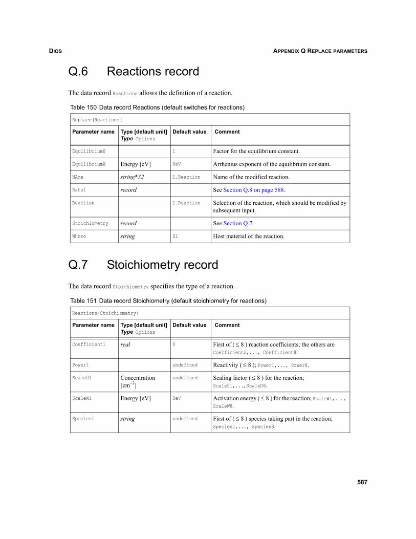
DIOS APPENDIX Q REPLACE PARAMETERS
Q.6 Reactions recordThe data record Reactions allows the definition of a reaction.
Q.7 Stoichiometry recordThe data record Stoichiometry specifies the type of a reaction.
Table 150 Data record Reactions (default switches for reactions)
Replace(Reactions(
Parameter name Type [default unit]Type Options
Default value Comment
Equilibrium0 1 Factor for the equilibrium constant.
EquilibriumW Energy [eV] 0eV Arrhenius exponent of the equilibrium constant.
NAme string*32 1.Reaction Name of the modified reaction.
Rate1 record See Section Q.8 on page 588.
Reaction 1.Reaction Selection of the reaction, which should be modified by subsequent input.
Stoichiometry record See Section Q.7.
Where string Si Host material of the reaction.
Table 151 Data record Stoichiometry (default stoichiometry for reactions)
Reactions(Stoichiometry(
Parameter name Type [default unit]Type Options
Default value Comment
Coefficient1 real 0 First of ( ) reaction coefficients; the others are Coefficient2,..., Coefficient8.
Power1 undefined Reactivity ( ); Power1,..., Power8.
Scale01 Concentration [cm–3]
undefined Scaling factor ( ) for the reaction; Scale01,...,ScaleO8.
ScaleW1 Energy [eV] 0eV Activation energy ( ) for the reaction; ScaleW1,..., ScaleW8.
Species1 string undefined First of ( ) species taking part in the reaction; Species1,..., Species8.
8≤
8≤
8≤
8≤
8≤
587

DIOSAPPENDIX Q REPLACE PARAMETERS
Q.8 Rate1 recordThe data record Rate1 specifies the rates of a reaction, compare Section 10.2.13 on page 198 and Eq. 202.Similar data records are Rate2...Rate4
Table 152 Data record Rate1 (default rates for reactions)
Reactions(Rate1(
Parameter name Type [default unit]Type Options
Default value Comment
Location string Numerator
Power1 real 0
Power2 real 0
Power3 real 0
Rate0 ReactionCoefficient [cm–3/s] undefined
RateW Energy [eV] 0eV
Scale01 Concentration [cm–3] undefined
Scale02 Concentration [cm–3] undefined
Scale03 Concentration [cm–3] undefined
ScaleW1 Energy [eV] 0eV
ScaleW2 Energy [eV] 0eV
ScaleW3 Energy [eV] 0eV
Species1 string undefined
Species2 string undefined
Species3 string undefined
588
DIOS APPENDIX R REFLECT PARAMETERS
Dios
APPENDIX R Reflect parameters
R.1 OverviewWith Dios, only half of a symmetric structure can be simulated. The Reflect command is used to expand,shrink, shift, or reflect the layer structure, the grid, the functions defined on the grid and, if possible, therefinement rectangles. The symmetry line must be at the left or right boundary or outside of the structure,resp. the chosen window. If the reflect line is outside of the existing structure, an 1D part is inserted, forexample, the gate length is ‘stretched.’
The Reflect command can be used repeatedly, but only one reflection at either the left or right side isallowed per Reflect command. It may be necessary to apply the command several times in order to avoidambiguous situations. Lateral and vertical 1D continuation, resp. reflection is applied to the profiles, noextrapolation is performed.
Besides reflecting, a structure can be stretched at a certain x-location (Xloc) to the right by use of theparameters in the Reflect(stretch( record. Here, Xloc determines where the structure is cut and Lengthdetermines how far the structure must be ‘stretched’ to the right. Profiles in the newly generated regionare given by the profile at the cutline:
Reflect(Stretch(Xloc=1um Length=0.5um))
The above command extends a given structure at position x=1 μm by 0.5 μm to the right. Xloc must beinside of the initial structure.
A ‘combination’ of several Dios layer structures is not foreseen in the reflect command, this must bedone in Mdraw, or using the LControl command (see Appendix U on page 597) (but, of course, analyticprofiles can be loaded after using the Reflect command to expand the Dios structure and grid).
Reflect(Window(Left Right Top Bottom=...),Reflect Shift VShift=...
)
During the Reflect command, the layer structure is reflected exactly. The user-defined refinement boxesare ‘reflected’ and the grid parameters are adjusted. Usually, a new grid is generated, starting with anadjusted user grid and performing a complete mesh adaptation.
NOTE A nonsymmetry in the final mesh after the reflection may be caused by the intersection of thefinal mesh adaptation tree with the (original plus reflected) material boundaries. Thisoperation does not respect any symmetry or periodicity of the structure. Due to round-offerrors, in rare cases, even the interpolated data may become nonsymmetric. The reason forthis is mostly a poor mesh quality in the mesh just before the reflection. This can be adjustedby the user.
589
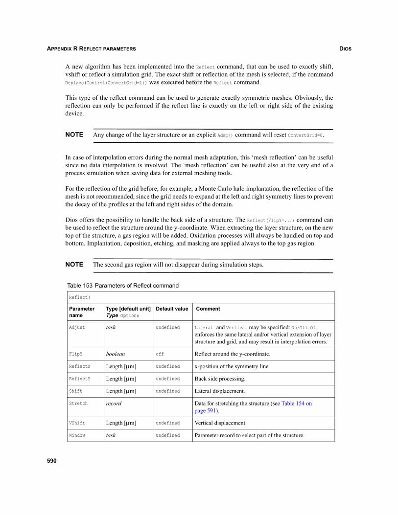
DIOSAPPENDIX R REFLECT PARAMETERS
A new algorithm has been implemented into the Reflect command, that can be used to exactly shift,vshift or reflect a simulation grid. The exact shift or reflection of the mesh is selected, if the commandReplace(Control(ConvertGrid=1)) was executed before the Reflect command.
This type of the reflect command can be used to generate exactly symmetric meshes. Obviously, thereflection can only be performed if the reflect line is exactly on the left or right side of the existingdevice.
NOTE Any change of the layer structure or an explicit Adap() command will reset ConvertGrid=0.
In case of interpolation errors during the normal mesh adaptation, this ‘mesh reflection’ can be usefulsince no data interpolation is involved. The ‘mesh reflection’ can be useful also at the very end of aprocess simulation when saving data for external meshing tools.
For the reflection of the grid before, for example, a Monte Carlo halo implantation, the reflection of themesh is not recommended, since the grid needs to expand at the left and right symmetry lines to preventthe decay of the profiles at the left and right sides of the domain.
Dios offers the possibility to handle the back side of a structure. The Reflect(FlipY=...) command canbe used to reflect the structure around the y-coordinate. When extracting the layer structure, on the newtop of the structure, a gas region will be added. Oxidation processes will always be handled on top andbottom. Implantation, deposition, etching, and masking are applied always to the top gas region.
NOTE The second gas region will not disappear during simulation steps.
Table 153 Parameters of Reflect command
Reflect(
Parameter name
Type [default unit]Type Options
Default value Comment
Adjust task undefined Lateral and Vertical may be specified: On/Off. Off enforces the same lateral and/or vertical extension of layer structure and grid, and may result in interpolation errors.
FlipY boolean off Reflect around the y-coordinate.
ReflectX Length [μm] undefined x-position of the symmetry line.
ReflectY Length [μm] undefined Back side processing.
Shift Length [μm] undefined Lateral displacement.
Stretch record Data for stretching the structure (see Table 154 on page 591).
VShift Length [μm] undefined Vertical displacement.
Window task undefined Parameter record to select part of the structure.
590
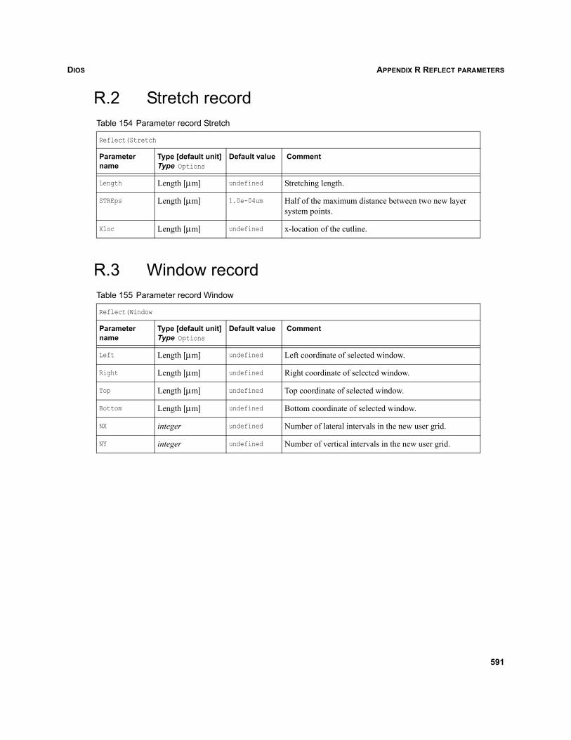
DIOS APPENDIX R REFLECT PARAMETERS
R.2 Stretch record
R.3 Window record
Table 154 Parameter record Stretch
Reflect(Stretch
Parameter name
Type [default unit]Type Options
Default value Comment
Length Length [μm] undefined Stretching length.
STREps Length [μm] 1.0e-04um Half of the maximum distance between two new layer system points.
Xloc Length [μm] undefined x-location of the cutline.
Table 155 Parameter record Window
Reflect(Window
Parameter name
Type [default unit]Type Options
Default value Comment
Left Length [μm] undefined Left coordinate of selected window.
Right Length [μm] undefined Right coordinate of selected window.
Top Length [μm] undefined Top coordinate of selected window.
Bottom Length [μm] undefined Bottom coordinate of selected window.
NX integer undefined Number of lateral intervals in the new user grid.
NY integer undefined Number of vertical intervals in the new user grid.
591

DIOSAPPENDIX R REFLECT PARAMETERS
592
DIOS APPENDIX S TCONTROL PARAMETERS
Dios
APPENDIX S TControl parameters
S.1 OverviewAfter using Ctrl+C in the command input window or clicking the break button in the X11 window, Diosenters the TControl mode. The program execution is continued if a closing parenthesis is entered or ifthe go button is clicked in the X11 window. The TControl mode can be used for interactive checks ofthe simulation result during the simulation of processing steps. The Graphic, Print, Save, 1D, LControl, andReplace commands can be used in this mode. The Adaptation command cannot be used in the TControlmode, but users can specify Replace(Control(Lada=1)) to enforce readaptation at the end of the currenttime step.
In addition, the parameters break, EBreak, Test, and After can be specified. To stop in the TControl modeagain, after the next time step, Test=on must be specified. You can also specify Test:=on as a new defaultvalue. Test=off or Test:=off return to the default mode. The TControl mode can be re-entered after acertain number of time steps: After=5.
If break is specified, the interpretation of the command file is stopped and the interactive mode is enteredwhen the running process step is finished. This has the same effect as if the break command were in thecommand file after the currently executed command. If EBreak is specified, the program enters theinteractive mode at the end of each process step.
The TControl mode is left usually with a closing parenthesis. When leaving TControl with quit, thecurrent process step is cancelled.
When leaving TControl with exit, stop, or end, the entire simulation is aborted (the same as double-clicking the exit button in the graphics window).
NOTE During a process step with no internal time loop or if only the last time step is running, theprogram may not stop in the TControl mode, but in the main command interpreter mode, asif a break command were in the command file. This is indicated only by the different prompt:TControl> or dios>.
593
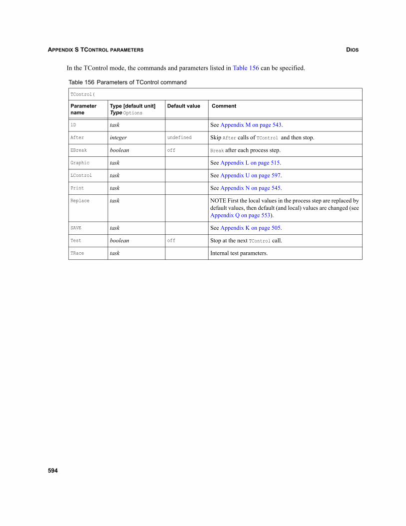
DIOSAPPENDIX S TCONTROL PARAMETERS
In the TControl mode, the commands and parameters listed in Table 156 can be specified.
Table 156 Parameters of TControl command
TControl(
Parameter name
Type [default unit]Type Options
Default value Comment
1D task See Appendix M on page 543.
After integer undefined Skip After calls of TControl and then stop.
EBreak boolean off Break after each process step.
Graphic task See Appendix L on page 515.
LControl task See Appendix U on page 597.
Print task See Appendix N on page 545.
Replace task NOTE First the local values in the process step are replaced by default values, then default (and local) values are changed (see Appendix Q on page 553).
SAVE task See Appendix K on page 505.
Test boolean off Stop at the next TControl call.
TRace task Internal test parameters.
594
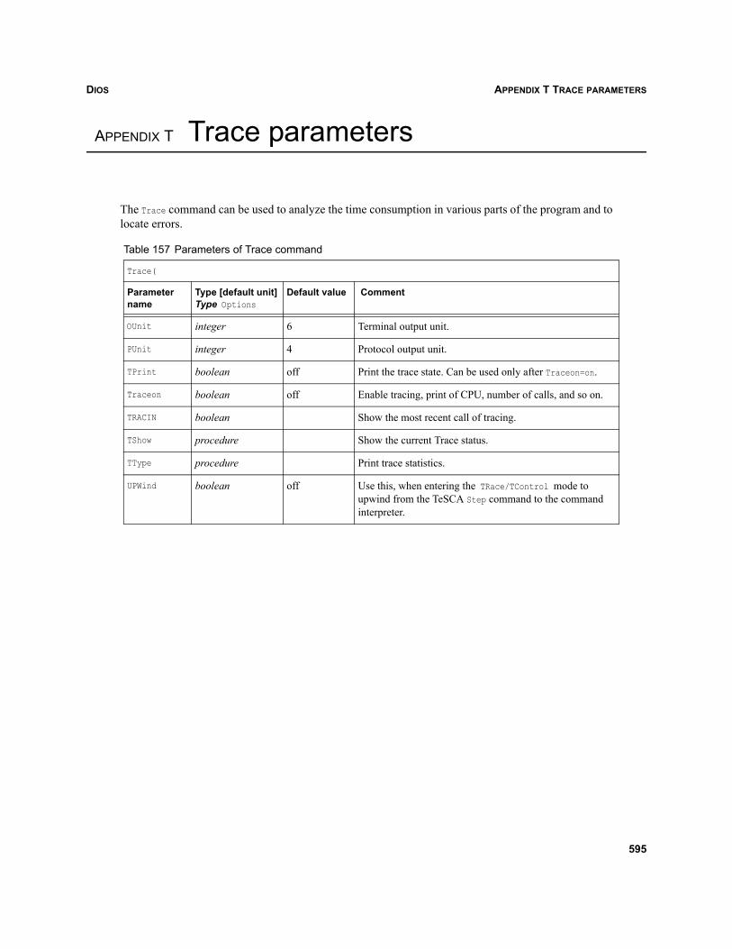
DIOS APPENDIX T TRACE PARAMETERS
Dios
APPENDIX T Trace parameters
The Trace command can be used to analyze the time consumption in various parts of the program and tolocate errors.
Table 157 Parameters of Trace command
Trace(
Parameter name
Type [default unit]Type Options
Default value Comment
OUnit integer 6 Terminal output unit.
PUnit integer 4 Protocol output unit.
TPrint boolean off Print the trace state. Can be used only after Traceon=on.
Traceon boolean off Enable tracing, print of CPU, number of calls, and so on.
TRACIN boolean Show the most recent call of tracing.
TShow procedure Show the current Trace status.
TType procedure Print trace statistics.
UPWind boolean off Use this, when entering the TRace/TControl mode to upwind from the TeSCA Step command to the command interpreter.
595

DIOSAPPENDIX T TRACE PARAMETERS
596
DIOS APPENDIX U LCONTROL PARAMETERS
Dios
APPENDIX U LControl parameters
U.1 OverviewThis command is used to check, draw, and manipulate the layer system. It should be used only in veryspecial situations, for example, if the commonly used commands fail and the user wants to analyze orsave the simulation. Some of the output and renaming operations may be useful to the user. It is notrecommended to use the command by default, since the concentrations are treated inconsistently andsome of the operations are not sufficiently robust.
Most of the subcommands work with ‘current’ values. New values can be specified explicitly or the=previous and =next commands can be used to modify the current values. The *set commands are usedto rename a material or boundary sort or the point coordinates. The *new and *del commands create ordelete various objects. Load and Save are used to save and load all existing complexes in binary form; Readand Write are used to save and load the current complex as an ASCII file. The complex can be modifiedusing the commands:
Copy Duplicates the current layer system.
Cut Cuts the specified material with a polygon, and replaces part of the materialwith a new one.
Shift Shifts and reflects the current complex.
Window Selects a window from the current complex.
Glue Merges two complexes with approximately the same left and right boundariesinto a new complex.
To manipulate an entire device, save the doping profiles: Save(File=xxx,Type=exp). Then, execute the Copy,Shift, Load, or Glue operations. To save the result, use one of the following commands:
SAVE(TYPe=lay,file=...)SAVE(TYPe=lai, file=...)LControl(SAVE(...)) LControl(WRITE(...))
Next, create a new mesh Grid and, in the last step, load and interpolate the doping profiles withappropriate symmetry and window specifications. The saved complex can also be loaded in the Substratecommand of a new next simulation run.
597
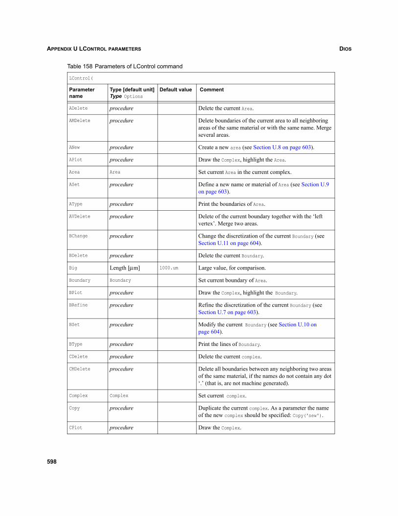
DIOSAPPENDIX U LCONTROL PARAMETERS
Table 158 Parameters of LControl command
LControl(
Parameter name
Type [default unit]Type Options
Default value Comment
ADelete procedure Delete the current Area.
AMDelete procedure Delete boundaries of the current area to all neighboring areas of the same material or with the same name. Merge several areas.
ANew procedure Create a new area (see Section U.8 on page 603).
APlot procedure Draw the Complex, highlight the Area.
Area Area Set current Area in the current complex.
ASet procedure Define a new name or material of Area (see Section U.9 on page 603).
AType procedure Print the boundaries of Area.
AVDelete procedure Delete of the current boundary together with the ‘left vertex’. Merge two areas.
BChange procedure Change the discretization of the current Boundary (see Section U.11 on page 604).
BDelete procedure Delete the current Boundary.
Big Length [μm] 1000.um Large value, for comparison.
Boundary Boundary Set current boundary of Area.
BPlot procedure Draw the Complex, highlight the Boundary.
BRefine procedure Refine the discretization of the current Boundary (see Section U.7 on page 603).
BSet procedure Modify the current Boundary (see Section U.10 on page 604).
BType procedure Print the lines of Boundary.
CDelete procedure Delete the current complex.
CMDelete procedure Delete all boundaries between any neighboring two areas of the same material, if the names do not contain any dot ‘.’ (that is, are not machine generated).
Complex Complex Set current complex.
Copy procedure Duplicate the current complex. As a parameter the name of the new complex should be specified: Copy('new').
CPlot procedure Draw the Complex.
598
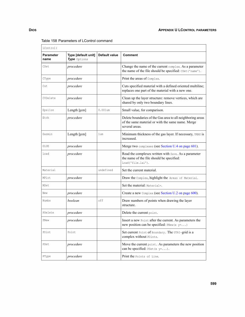
DIOS APPENDIX U LCONTROL PARAMETERS
CSet procedure Change the name of the current complex. As a parameter the name of the file should be specified: CSet('name').
CType procedure Print the areas of Complex.
Cut procedure Cuts specified material with a defined oriented multiline; replaces one part of the material with a new one.
CVDelete procedure Clean up the layer structure: remove vertices, which are shared by only two boundary lines.
Epsilon Length [μm] 0.001um Small value, for comparison.
Etch procedure Delete boundaries of the Gas area to all neighboring areas of the same material or with the same name. Merge several areas.
Gasmin Length [μm] 1um Minimum thickness of the gas layer. If necessary, YMAX is increased.
GLUE procedure Merge two complexes (see Section U.4 on page 601).
Load procedure Read the complexes written with Save. As a parameter the name of the file should be specified: Load('file.lai').
Material undefined Set the current material.
MPlot procedure Draw the Complex, highlight the Areas of Material.
MSet Set the material: Material=.
New procedure Create a new Complex (see Section U.2 on page 600).
Numbs boolean off Draw numbers of points when drawing the layer structure.
PDelete procedure Delete the current point.
PNew procedure Insert a new Point after the current. As parameters the new position can be specified: PNew(x y=...)
POint Point Set current Point of Boundary. The UTRI-grid is a complex without POints.
PSet procedure Move the current point. As parameters the new position can be specified: PSet(x y=...).
PType procedure Print the Points of Line.
Table 158 Parameters of LControl command
LControl(
Parameter name
Type [default unit]Type Options
Default value Comment
599
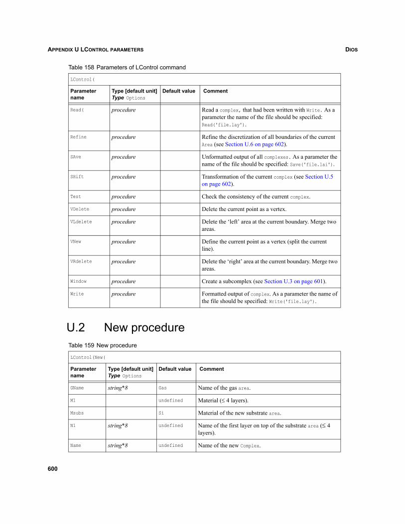
DIOSAPPENDIX U LCONTROL PARAMETERS
U.2 New procedure
Read( procedure Read a complex, that had been written with Write. As a parameter the name of the file should be specified: Read('file.lay').
Refine procedure Refine the discretization of all boundaries of the current Area (see Section U.6 on page 602).
SAve procedure Unformatted output of all complexes. As a parameter the name of the file should be specified: Save('file.lai').
SHift procedure Transformation of the current complex (see Section U.5 on page 602).
Test procedure Check the consistency of the current complex.
VDelete procedure Delete the current point as a vertex.
VLdelete procedure Delete the ‘left’ area at the current boundary. Merge two areas.
VNew procedure Define the current point as a vertex (split the current line).
VRdelete procedure Delete the ‘right’ area at the current boundary. Merge two areas.
Window procedure Create a subcomplex (see Section U.3 on page 601).
Write procedure Formatted output of complex. As a parameter the name of the file should be specified: Write('file.lay').
Table 159 New procedure
LControl(New(
Parameter name
Type [default unit]Type Options
Default value Comment
GName string*8 Gas Name of the gas area.
M1 undefined Material (≤ 4 layers).
Msubs Si Material of the new substrate area.
N1 string*8 undefined Name of the first layer on top of the substrate area (≤ 4 layers).
Name string*8 undefined Name of the new Complex.
Table 158 Parameters of LControl command
LControl(
Parameter name
Type [default unit]Type Options
Default value Comment
600
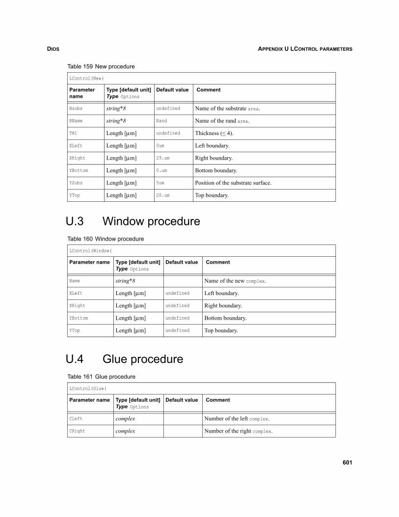
DIOS APPENDIX U LCONTROL PARAMETERS
U.3 Window procedure
U.4 Glue procedure
Nsubs string*8 undefined Name of the substrate area.
RName string*8 Rand Name of the rand area.
TH1 Length [μm] undefined Thickness (< 4).
XLeft Length [μm] 0um Left boundary.
XRight Length [μm] 29.um Right boundary.
YBottom Length [μm] 0.um Bottom boundary.
YSubs Length [μm] 5um Position of the substrate surface.
YTop Length [μm] 20.um Top boundary.
Table 160 Window procedure
LControl(Window(
Parameter name Type [default unit]Type Options
Default value Comment
Name string*8 Name of the new complex.
XLeft Length [μm] undefined Left boundary.
XRight Length [μm] undefined Right boundary.
YBottom Length [μm] undefined Bottom boundary.
YTop Length [μm] undefined Top boundary.
Table 161 Glue procedure
LControl(Glue(
Parameter name Type [default unit]Type Options
Default value Comment
CLeft complex Number of the left complex.
CRight complex Number of the right complex.
Table 159 New procedure
LControl(New(
Parameter name
Type [default unit]Type Options
Default value Comment
601
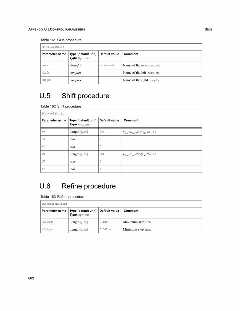
DIOSAPPENDIX U LCONTROL PARAMETERS
U.5 Shift procedure
U.6 Refine procedure
NAme string*8 undefined Name of the new complex.
NLeft complex Name of the left complex.
NRight complex Name of the right complex.
Table 162 Shift procedure
LControl(Shift(
Parameter name Type [default unit]Type Options
Default value Comment
X0 Length [μm] 0um xnew=xold XX+yold XY +X0
XX real 1
XY real 0
Y0 Length [μm] 0um ynew=xold YX+yold YY +Y0
YX real 0
YY real 1
Table 163 Refine procedure
LControl(Refine(
Parameter name Type [default unit]Type Options
Default value Comment
MAximum Length [μm] 0.1um Maximum step size.
MInimum Length [μm] 0.001um Minimum step size.
Table 161 Glue procedure
LControl(Glue(
Parameter name Type [default unit]Type Options
Default value Comment
602
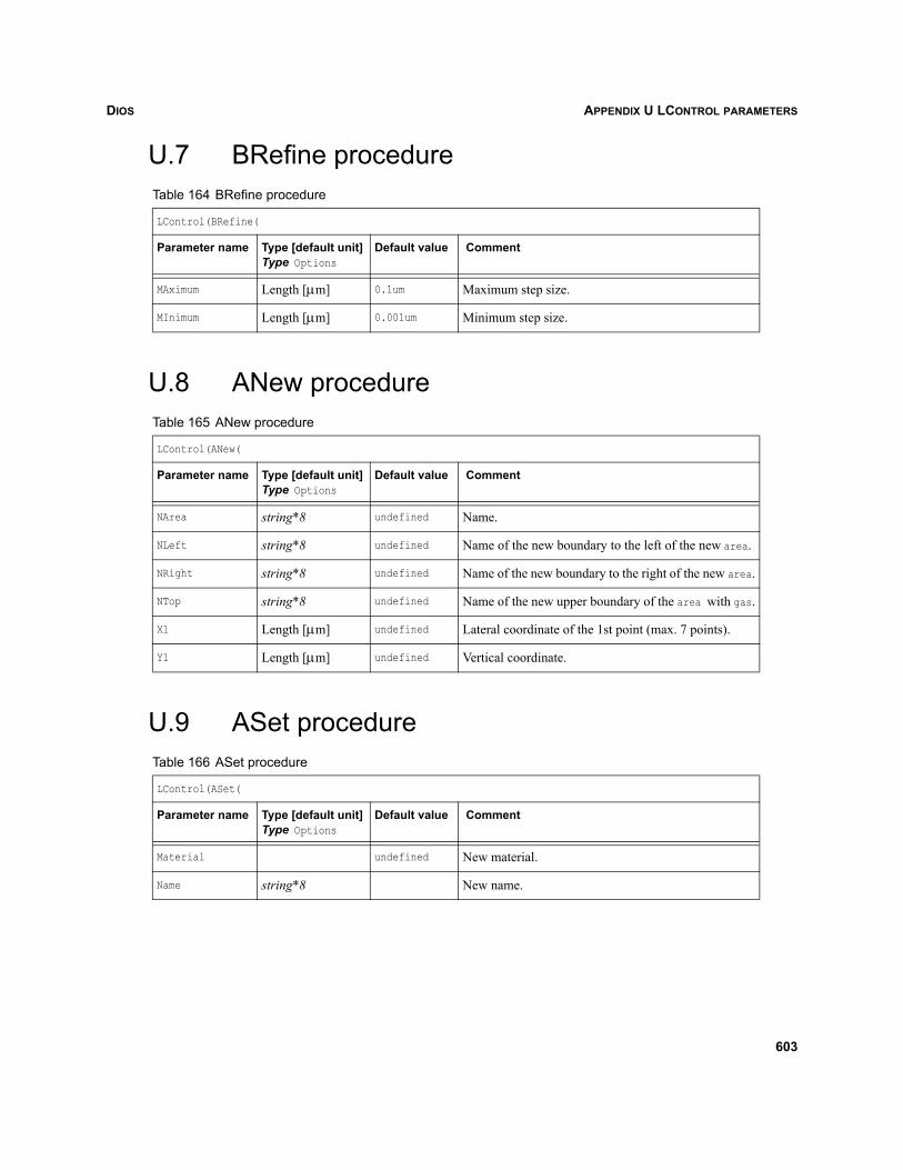
DIOS APPENDIX U LCONTROL PARAMETERS
U.7 BRefine procedure
U.8 ANew procedure
U.9 ASet procedure
Table 164 BRefine procedure
LControl(BRefine(
Parameter name Type [default unit]Type Options
Default value Comment
MAximum Length [μm] 0.1um Maximum step size.
MInimum Length [μm] 0.001um Minimum step size.
Table 165 ANew procedure
LControl(ANew(
Parameter name Type [default unit]Type Options
Default value Comment
NArea string*8 undefined Name.
NLeft string*8 undefined Name of the new boundary to the left of the new area.
NRight string*8 undefined Name of the new boundary to the right of the new area.
NTop string*8 undefined Name of the new upper boundary of the area with gas.
X1 Length [μm] undefined Lateral coordinate of the 1st point (max. 7 points).
Y1 Length [μm] undefined Vertical coordinate.
Table 166 ASet procedure
LControl(ASet(
Parameter name Type [default unit]Type Options
Default value Comment
Material undefined New material.
Name string*8 New name.
603
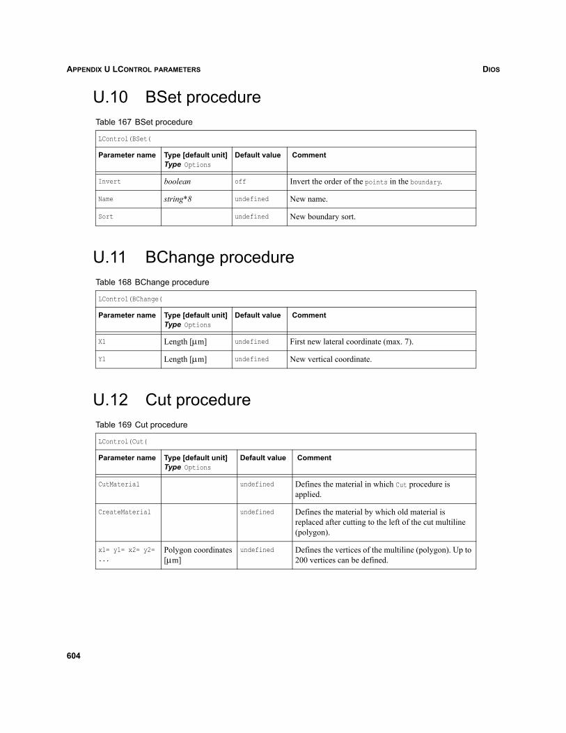
DIOSAPPENDIX U LCONTROL PARAMETERS
U.10 BSet procedure
U.11 BChange procedure
U.12 Cut procedure
Table 167 BSet procedure
LControl(BSet(
Parameter name Type [default unit]Type Options
Default value Comment
Invert boolean off Invert the order of the points in the boundary.
Name string*8 undefined New name.
Sort undefined New boundary sort.
Table 168 BChange procedure
LControl(BChange(
Parameter name Type [default unit]Type Options
Default value Comment
X1 Length [μm] undefined First new lateral coordinate (max. 7).
Y1 Length [μm] undefined New vertical coordinate.
Table 169 Cut procedure
LControl(Cut(
Parameter name Type [default unit]Type Options
Default value Comment
CutMaterial undefined Defines the material in which Cut procedure is applied.
CreateMaterial undefined Defines the material by which old material is replaced after cutting to the left of the cut multiline (polygon).
x1= y1= x2= y2=...
Polygon coordinates [μm]
undefined Defines the vertices of the multiline (polygon). Up to 200 vertices can be defined.
604
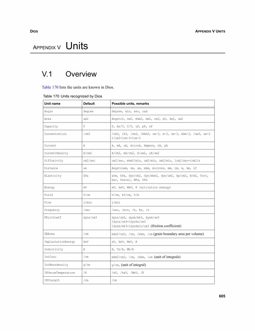
DIOS APPENDIX V UNITS
Dios
APPENDIX V Units
V.1 OverviewTable 170 lists the units are known in Dios.
Table 170 Units recognized by Dios
Unit name Default Possible units, remarks
Angle degree degree, min, sec, rad
Area um2 Angstr2, nm2, mkm2, mm2, cm2, m2, km2, um2
Capacity F F, As/V, C/V, uF, pF, nF
Concentration /cm3 /cm3, /m3, /nm3, /mkm3, cm-3, m-3, nm-3, mkm-3, /um3, um-31/cm3=1cm-3=1cm-3
Current A A, mA, uA, microA, Ampere, nA, pA
CurrentDensity A/cm2 A/cm2, mA/cm2, A/um2, uA/um2
Diffusivity cm2/sec cm2/sec, mkm2/min, um2/min, nm2/min, 1cm2/sec=1cm2/s
Distance um Angstroem, nm, um, mkm, microns, mm, cm, m, km, LY
ELasticity GPa atm, hPa, dyn/cm2, dyn/mkm2, dyn/um2, kp/cm2, N/m2, Torr, bar, Pascal, MPa, GPa
Energy eV eV, keV, MeV, K (activation energy)
Field V/cm V/cm, kV/cm, V/m
Flow l/min l/min
Frequency /sec /sec, /min, /h, Hz, /s
FRictCoeff dyns/cm3 dyns/cm3, dynm/mk3, dynm/um31dyns/cm3=1dynÞs/cm31dynm/mk3=1dynÞmin/um3 (friction coefficient)
GBArea /um mkm2/cm3, /cm, /mkm, /um (grain boundary area per volume)
ImplantationEnergy keV eV, keV, MeV, K
Inductivity H H, Vs/A, Wb/A
IntConc /cm mkm2/cm3, /cm, /mkm, /um (unit of integrals)
IntMassdensity g/cm g/cm, (unit of integral)
INVerseTemperature /K /eV, /keV, /MeV, /K
INVLength /cm /cm
605
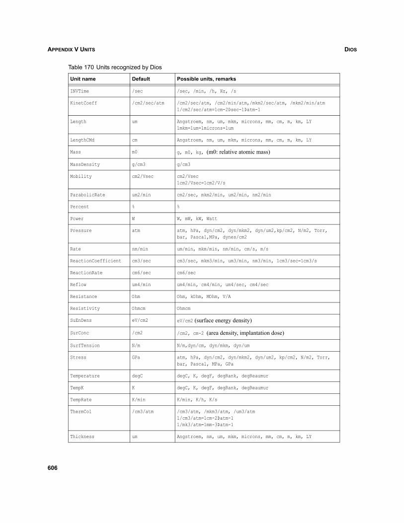
DIOSAPPENDIX V UNITS
INVTime /sec /sec, /min, /h, Hz, /s
KinetCoeff /cm2/sec/atm /cm2/sec/atm, /cm2/min/atm,/mkm2/sec/atm, /mkm2/min/atm1/cm2/sec/atm=1cm-2Þsec-1Þatm-1
Length um Angstroem, nm, um, mkm, microns, mm, cm, m, km, LY1mkm=1um=1microns=1um
LengthCMd cm Angstroem, nm, um, mkm, microns, mm, cm, m, km, LY
Mass m0 g, m0, kg, (m0: relative atomic mass)
MassDensity g/cm3 g/cm3
Mobility cm2/Vsec cm2/Vsec1cm2/Vsec=1cm2/V/s
ParabolicRate um2/min cm2/sec, mkm2/min, um2/min, nm2/min
Percent % %
Power W W, mW, kW, Watt
Pressure atm atm, hPa, dyn/cm2, dyn/mkm2, dyn/um2,kp/cm2, N/m2, Torr, bar, Pascal,MPa, dynes/cm2
Rate nm/min um/min, mkm/min, nm/min, cm/s, m/s
ReactionCoefficient cm3/sec cm3/sec, mkm3/min, um3/min, nm3/min, 1cm3/sec=1cm3/s
ReactionRate cm6/sec cm6/sec
Reflow um4/min um4/min, cm4/min, um4/sec, cm4/sec
Resistance Ohm Ohm, kOhm, MOhm, V/A
Resistivity Ohmcm Ohmcm
SuEnDens eV/cm2 eV/cm2 (surface energy density)
SurConc /cm2 /cm2, cm-2 (area density, implantation dose)
SurfTension N/m N/m,dyn/cm, dyn/mkm, dyn/um
Stress GPa atm, hPa, dyn/cm2, dyn/mkm2, dyn/um2, kp/cm2, N/m2, Torr, bar, Pascal, MPa, GPa
Temperature degC degC, K, degF, degRank, degReaumur
TempK K degC, K, degF, degRank, degReaumur
TempRate K/min K/min, K/h, K/s
ThermCo1 /cm3/atm /cm3/atm, /mkm3/atm, /um3/atm1/cm3/atm=1cm-2Þatm-11/mk3/atm=1mm-3Þatm-1
Thickness um Angstroem, nm, um, mkm, microns, mm, cm, m, km, LY
Table 170 Units recognized by Dios
Unit name Default Possible units, remarks
606
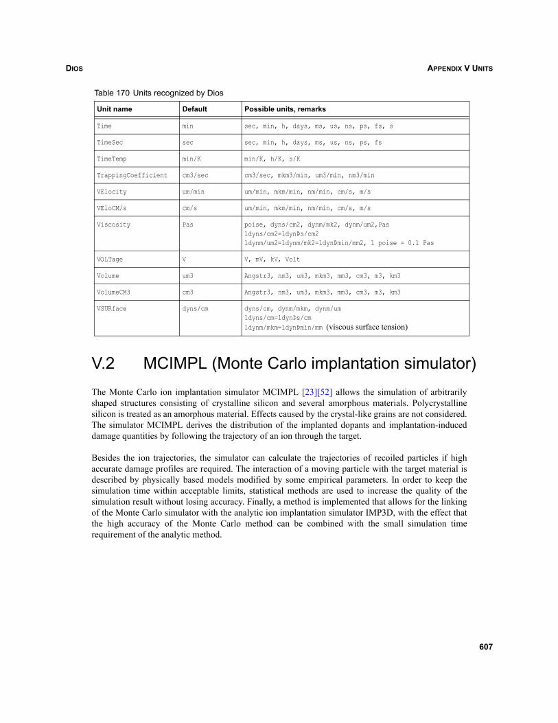
DIOS APPENDIX V UNITS
V.2 MCIMPL (Monte Carlo implantation simulator)The Monte Carlo ion implantation simulator MCIMPL [23][52] allows the simulation of arbitrarilyshaped structures consisting of crystalline silicon and several amorphous materials. Polycrystallinesilicon is treated as an amorphous material. Effects caused by the crystal-like grains are not considered.The simulator MCIMPL derives the distribution of the implanted dopants and implantation-induceddamage quantities by following the trajectory of an ion through the target.
Besides the ion trajectories, the simulator can calculate the trajectories of recoiled particles if highaccurate damage profiles are required. The interaction of a moving particle with the target material isdescribed by physically based models modified by some empirical parameters. In order to keep thesimulation time within acceptable limits, statistical methods are used to increase the quality of thesimulation result without losing accuracy. Finally, a method is implemented that allows for the linkingof the Monte Carlo simulator with the analytic ion implantation simulator IMP3D, with the effect thatthe high accuracy of the Monte Carlo method can be combined with the small simulation timerequirement of the analytic method.
Time min sec, min, h, days, ms, us, ns, ps, fs, s
TimeSec sec sec, min, h, days, ms, us, ns, ps, fs
TimeTemp min/K min/K, h/K, s/K
TrappingCoefficient cm3/sec cm3/sec, mkm3/min, um3/min, nm3/min
VElocity um/min um/min, mkm/min, nm/min, cm/s, m/s
VEloCM/s cm/s um/min, mkm/min, nm/min, cm/s, m/s
Viscosity Pas poise, dyns/cm2, dynm/mk2, dynm/um2,Pas1dyns/cm2=1dynÞs/cm21dynm/um2=1dynm/mk2=1dynÞmin/mm2, 1 poise = 0.1 Pas
VOLTage V V, mV, kV, Volt
Volume um3 Angstr3, nm3, um3, mkm3, mm3, cm3, m3, km3
VolumeCM3 cm3 Angstr3, nm3, um3, mkm3, mm3, cm3, m3, km3
VSURface dyns/cm dyns/cm, dynm/mkm, dynm/um1dyns/cm=1dynÞs/cm1dynm/mkm=1dynÞmin/mm (viscous surface tension)
Table 170 Units recognized by Dios
Unit name Default Possible units, remarks
607
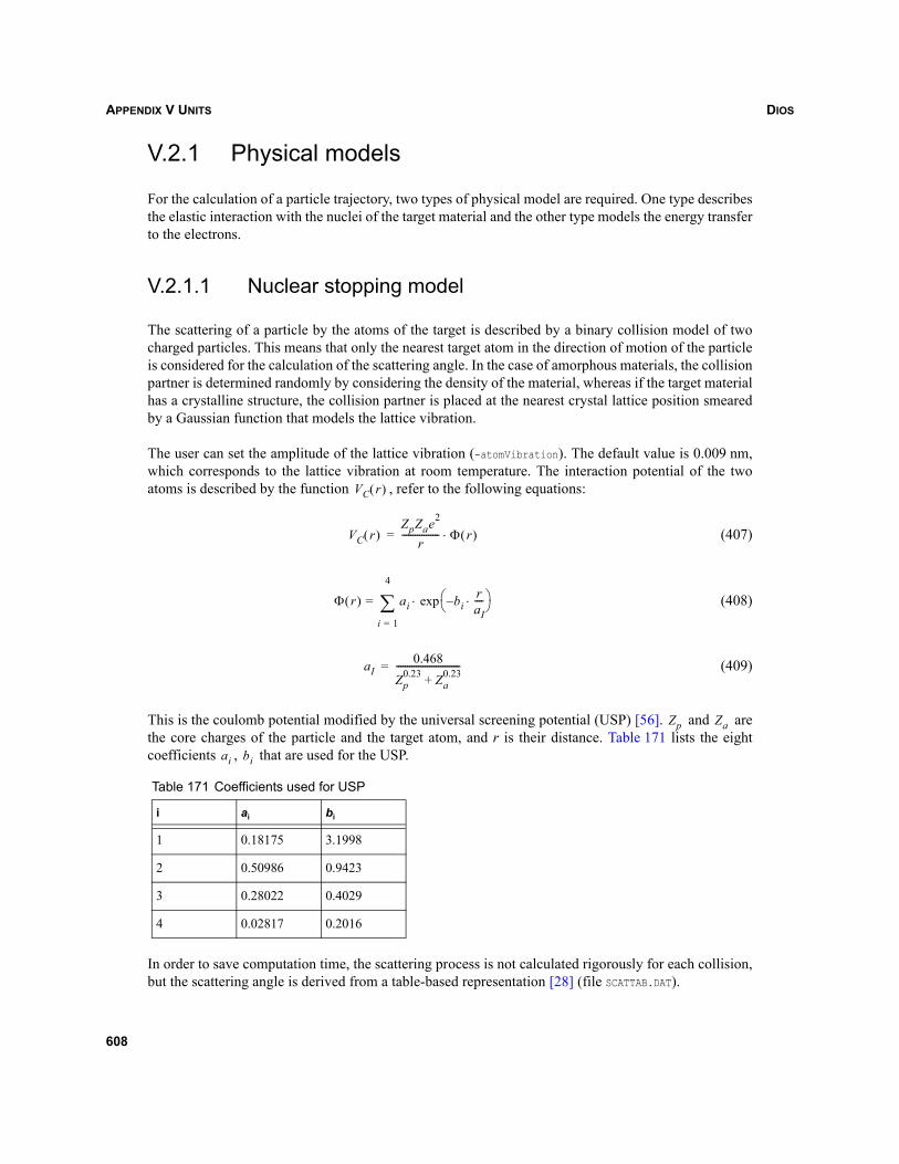
DIOSAPPENDIX V UNITS
V.2.1 Physical models
For the calculation of a particle trajectory, two types of physical model are required. One type describesthe elastic interaction with the nuclei of the target material and the other type models the energy transferto the electrons.
V.2.1.1 Nuclear stopping model
The scattering of a particle by the atoms of the target is described by a binary collision model of twocharged particles. This means that only the nearest target atom in the direction of motion of the particleis considered for the calculation of the scattering angle. In the case of amorphous materials, the collisionpartner is determined randomly by considering the density of the material, whereas if the target materialhas a crystalline structure, the collision partner is placed at the nearest crystal lattice position smearedby a Gaussian function that models the lattice vibration.
The user can set the amplitude of the lattice vibration (-atomVibration). The default value is 0.009 nm,which corresponds to the lattice vibration at room temperature. The interaction potential of the twoatoms is described by the function , refer to the following equations:
(407)
(408)
(409)
This is the coulomb potential modified by the universal screening potential (USP) [56]. and arethe core charges of the particle and the target atom, and r is their distance. Table 171 lists the eightcoefficients , that are used for the USP.
In order to save computation time, the scattering process is not calculated rigorously for each collision,but the scattering angle is derived from a table-based representation [28] (file SCATTAB.DAT).
Table 171 Coefficients used for USP
i ai bi
1 0.18175 3.1998
2 0.50986 0.9423
3 0.28022 0.4029
4 0.02817 0.2016
VC r( )
VC r( )ZpZae2
r----------------- Φ r( )⋅=
Φ r( ) ai biraI----⋅–⎝ ⎠
⎛ ⎞exp⋅
i 1=
4
∑=
aI0.468
Zp0.23 Za
0.23+-----------------------------=
Zp Za
ai bi
608
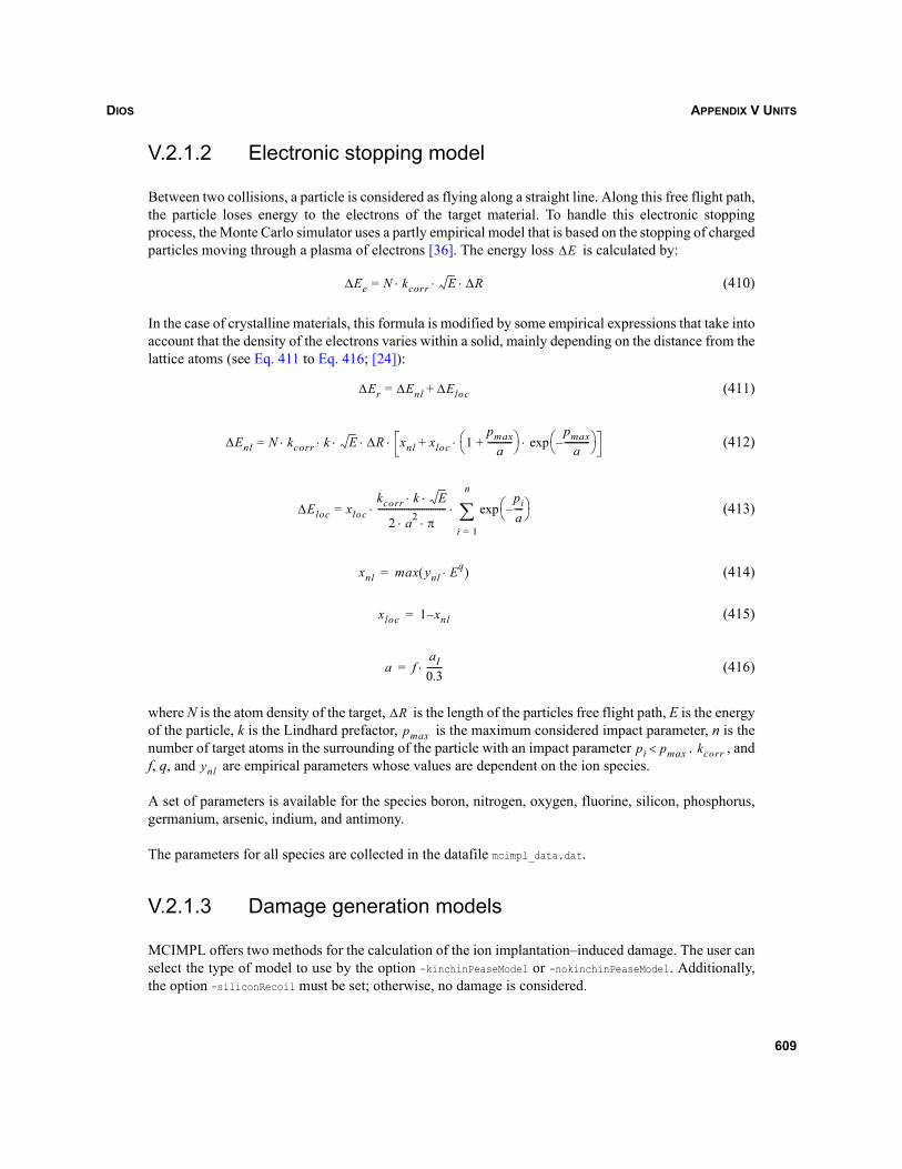
DIOS APPENDIX V UNITS
V.2.1.2 Electronic stopping model
Between two collisions, a particle is considered as flying along a straight line. Along this free flight path,the particle loses energy to the electrons of the target material. To handle this electronic stoppingprocess, the Monte Carlo simulator uses a partly empirical model that is based on the stopping of chargedparticles moving through a plasma of electrons [36]. The energy loss is calculated by:
(410)
In the case of crystalline materials, this formula is modified by some empirical expressions that take intoaccount that the density of the electrons varies within a solid, mainly depending on the distance from thelattice atoms (see Eq. 411 to Eq. 416; [24]):
(411)
(412)
(413)
(414)
(415)
(416)
where N is the atom density of the target, is the length of the particles free flight path, E is the energyof the particle, k is the Lindhard prefactor, is the maximum considered impact parameter, n is thenumber of target atoms in the surrounding of the particle with an impact parameter . , andf, q, and are empirical parameters whose values are dependent on the ion species.
A set of parameters is available for the species boron, nitrogen, oxygen, fluorine, silicon, phosphorus,germanium, arsenic, indium, and antimony.
The parameters for all species are collected in the datafile mcimpl_data.dat.
V.2.1.3 Damage generation models
MCIMPL offers two methods for the calculation of the ion implantation–induced damage. The user canselect the type of model to use by the option -kinchinPeaseModel or -nokinchinPeaseModel. Additionally,the option -siliconRecoil must be set; otherwise, no damage is considered.
ΔE
ΔEe N kcorr E ΔR⋅ ⋅ ⋅=
ΔEr ΔEnl ΔEloc+=
ΔEnl N kcorr k E ΔR xnl xloc 1pmax
a-----------+⎝ ⎠
⎛ ⎞ pmaxa
-----------–⎝ ⎠⎛ ⎞exp⋅ ⋅+⋅⋅ ⋅ ⋅ ⋅=
ΔEloc xlockcorr k E⋅ ⋅
2 a2 π⋅ ⋅-------------------------------
pia----–⎝ ⎠
⎛ ⎞expi 1=
n
∑⋅ ⋅=
xnl max ynl Eq⋅( )=
xloc 1 x– nl=
a faI0.3-------⋅=
ΔRpmax
pi pmax< kcorrynl
609
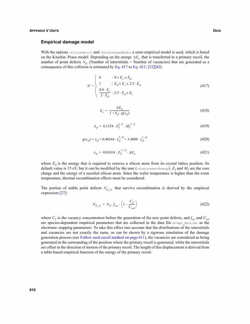
DIOSAPPENDIX V UNITS
Empirical damage model
With the options -siliconRecoil and -kinchinPeaseModel, a semi-empirical model is used, which is basedon the Kinchin–Pease model. Depending on the energy that is transferred to a primary recoil, thenumber of point defects (Number of interstitials = Number of vacancies) that are generated as aconsequence of this collision is estimated by Eq. 417 to Eq. 421; [32][42]:
(417)
(418)
(419)
(420)
(421)
where Ed is the energy that is required to remove a silicon atom from its crystal lattice position. Itsdefault value is 15 eV, but it can be modified by the user (-displacementEnergy). ZT and MT are the corecharge and the energy of a recoiled silicon atom. Since the wafer temperature is higher than the roomtemperature, thermal recombination effects must be considered.
The portion of stable point defects that survive recombination is derived by the empiricalexpression [27]:
(422)
where CV is the vacancy concentration before the generation of the new point defects, and frec and Csatare species-dependent empirical parameters that are collected in the data file mcimpl_data.dat as theelectronic stopping parameters. To take this effect into account that the distributions of the interstitialsand vacancies are not exactly the same, as can be shown by a rigorous simulation of the damagegeneration process (see Follow each recoil method on page 611), the vacancies are considered as beinggenerated in the surrounding of the position where the primary recoil is generated, while the interstitialsare offset in the direction of motion of the primary recoil. The length of this displacement is derived froma table-based empirical function of the energy of the primary recoil.
ΔEnNd
N
0 : 0 Ev Ed≤ ≤
1 : Ed Ev 2.5 Ed⋅≤ ≤
0.8 Ev⋅2 Ed⋅
----------------- : 2.5 Ed Ev≤⋅⎩⎪⎪⎨⎪⎪⎧
=
EvΔEn
1 kd g εd( )⋅+--------------------------------=
kd 0.1334 ZT2 3⁄ MT
1 2⁄–⋅ ⋅=
g εd( ) εd 0.40244 εd3 4⁄ 3.4008 εd
1 6⁄⋅+⋅+=
εd 0.01014 ZT7– 3⁄ ΔEn⋅ ⋅=
Nd_st
Nd_st Nd frec 1CV
Csat----------–⎝ ⎠
⎛ ⎞⋅ ⋅=
610
DIOS APPENDIX V UNITS
Follow each recoil method
Apart from the empirical damage model, a ‘follow each recoil’ method [28] can be used (-siliconRecoiland -nokinchinPeaseModel) to calculate more accurate vacancy and interstitial distributions. By using thismethod, the trajectories of the implanted ions and the trajectories of all recoiled silicon atoms arecalculated. A recoil is generated if the energy transferred during an elastic collision of a moving particle(implanted ion species or silicon atom) with a silicon atom is above the displacement energy Ed (seeEmpirical damage model on page 610).
In the case of crystalline materials, the recoiled atom can be either a lattice atom, which results in thegeneration of a vacancy and an interstitial, or a previously generated interstitial. The recoil type isselected randomly, where Eq. 423 sets the probability for using an interstitial:
(423)
where CI is the interstitial concentration and CM is the particle density of the target material. If a recoiledatom comes to rest, a statistical recombination model is applied to consider thermal effects. Theprobability prec for a recombination of the recoil with a previously generated vacancy is determined by:
(424)
where CV is the vacancy concentration and rrec is an empirical parameter (-capturingFactor), whichdescribes the recombination range of an interstitial before it comes to rest.
De-channeling and amorphization
The point defects generated during the ion implantation process influence the trajectories of theimplanted ions and the recoiled particles, because they modify or even destroy the crystalline structureof the material. This de-channeling effect is handled by randomly placing silicon atoms instead ofplacing them at a crystal lattice position. Eq. 425 gives the probability pran for a random placement:
(425)
If the point defect concentration exceeds the amorphization concentration , the target material istreated as being amorphous with the consequence that only randomly placed silicon atoms are used forthe trajectory calculation. Up to now, the amorphization concentration is an empirical parameter that theuser can set (-amorphizationLevel).
pRI
pRI
CICM--------=
prec rrecCVCM--------⋅=
pran
CI CV+CM
------------------- : CI CV Cα<+
1 : CI CV+ Cα>⎩⎪⎨⎪⎧
=
Cα
611
DIOSAPPENDIX V UNITS
V.2.2 Special features
V.2.2.1 Molecular ions
MCIMPL offers two methods for the simulation of the implantation of molecular ions [29]. With theoption -simpleMolecule respective to -nosimpleMolecule, either a simple method or a rigorous method canbe selected. By using the rigorous method, the distributions of all species in the molecule are calculated.For each species, the same empirical parameters (from the file mcimpl_data.dat) as for single atomic ionimplantations are used.
If the simple method is applied, only the distribution of one significant atom species of the molecule (forexample, boron in BF2) is calculated. For this method, an additional entry in the parameter filemcimpl_data.dat is required for the molecular species, because the influence of all other atoms in themolecule on the simulation result is considered by a modified damage generation property of thecalculated species. The simple method can only be used in combination with the Kinchin–Pease damagemodel. Two types of molecular ions are supported: BF2 and N2.
It is not possible to add new types of molecular ions by simply adding appropriate empirical parametersto the file mcimpl_data.dat, because the composition of the molecule and the type of the significantspecies are hard coded for all molecules.
V.2.2.2 Point-response interface
In order to combine the advantages of the Monte Carlo and the analytic ion implantation simulationmethod, MCIMPL offers the opportunity (-pointResponse) to calculate a point-response function for asignificant point (center of -implantationWindow) of the simulation domain. This point-response functionis stored in a file (*.RESP) and can be used by the analytic ion implantation simulator IMP3D to derivethe doping concentration for the complete simulation domain.
The size of the implantation window around the significant point should be at least as large as the verticalrange of the implanted ions; otherwise, an underestimation of the implantation-induced damage resultsin an incorrect doping profile. Even if the implantation window is quite large, the point-responsefunction is not blurred, because the simulation result is compressed to a single point when calculatingthe point-response function.
V.2.3 Speedup methods
In order to increase the speed of the simulation, two statistical methods are implemented that improvethe quality of the simulation result without significantly increasing the simulation time. Theconsequence is that the actual number of trajectories that must be calculated can be decreased withoutlosing statistical accuracy. Since the simulation time is proportional to the number of calculatedtrajectories, a speedup of the simulation is possible.
612
DIOS APPENDIX V UNITS
V.2.3.1 Trajectory split method
The statistical noise is all the higher the lower the concentration. The effect of the trajectory split methodis that a part of a trajectory leading through a region of high concentration is used for several effectivetrajectories. Thereby, the number of calculated collisions for one effective trajectory is significantlyreduced with the consequence of a decrease in the simulation time per effective trajectory. Moreover,the statistical noise of the simulation result is improved, because the effective trajectories mainly end inregions of low concentration.
By the trajectory split method [6], a physical particle is split into two virtual particles when it moves toa region of a lower concentration. These virtual particles physically behave like the original particle, butthe number of point defects that are produced by a virtual particle and their contribution to the finaldistribution of the particle species are weighted according to the number of virtual particles originatingfrom the same physical particle. This number can be larger than two because a virtual particle can alsobe split.
In order to work properly, the trajectory split method needs some information about the particledistribution. The user can define the number of primary trajectories (-nbPrimaryIons) that are used togenerate a rough distribution, before the trajectory split method is initiated. The number of primarytrajectories should be less than 10% of the total number of trajectories (-nbIons).
V.2.3.2 Trajectory reuse method
While the trajectory split method is applied within crystalline materials, a more efficient method isapplied within amorphous materials. Due to the isotropy and to the fact that the particles are notinfluenced by damage effects, a trajectory that is calculated once for a certain material type can be usedat several locations in the simulation domain.
This property is made use of by splitting the simulation domain into several subdomains. If a trajectorythrough a certain material is calculated for one subdomain, it can be reused for other subdomains on thecondition that the particle energy interval of the precalculated trajectory contains the entrance energy ofthe particle into the same material in the new subdomain. At best, only one trajectory for each subdomainhas to be calculated. The gain in simulation time is proportional to the number of subdomains and,thereby, to the size of the simulation domain, because the size of one subdomain is of the order of thevertical range of the implanted particles.
613

DIOSAPPENDIX V UNITS
614
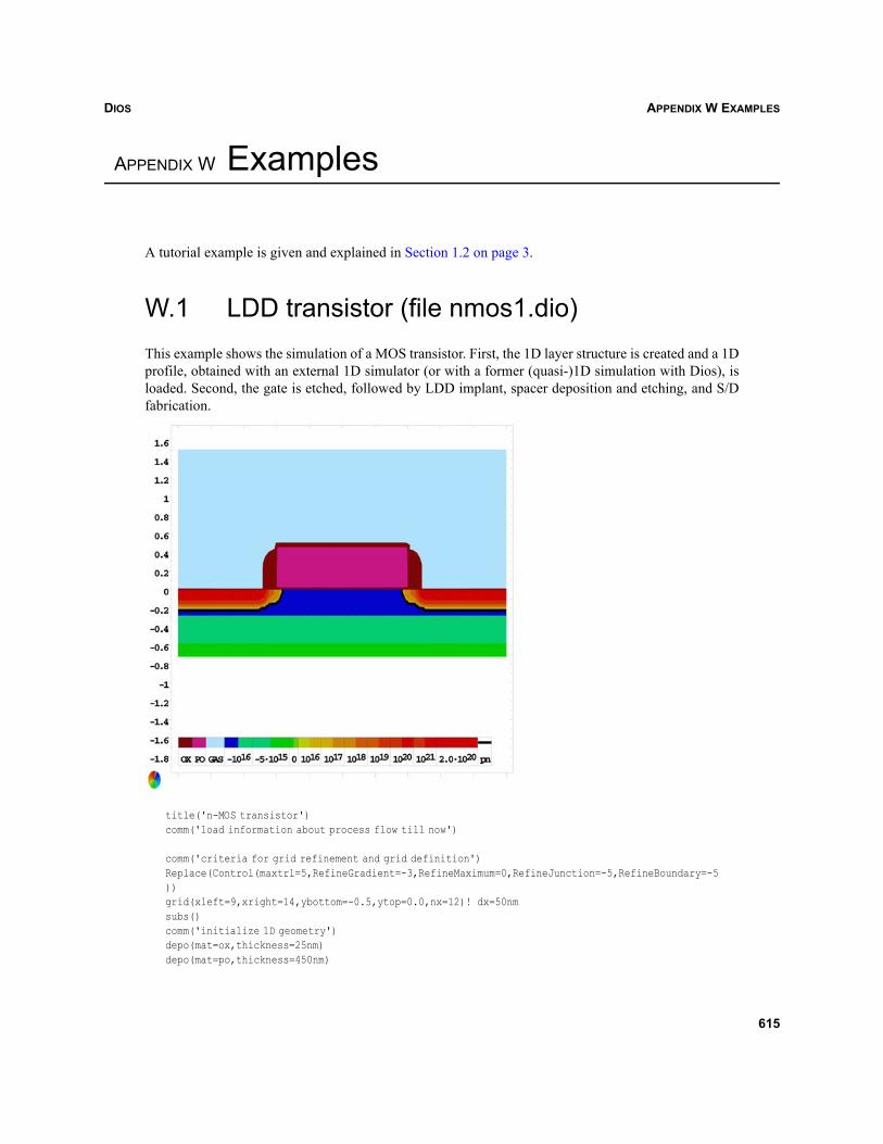
DIOS APPENDIX W EXAMPLES
Dios
APPENDIX W Examples
A tutorial example is given and explained in Section 1.2 on page 3.
W.1 LDD transistor (file nmos1.dio)This example shows the simulation of a MOS transistor. First, the 1D layer structure is created and a 1Dprofile, obtained with an external 1D simulator (or with a former (quasi-)1D simulation with Dios), isloaded. Second, the gate is etched, followed by LDD implant, spacer deposition and etching, and S/Dfabrication.
title('n-MOS transistor')comm('load information about process flow till now')
comm('criteria for grid refinement and grid definition')Replace(Control(maxtrl=5,RefineGradient=-3,RefineMaximum=0,RefineJunction=-5,RefineBoundary=-5))grid(xleft=9,xright=14,ybottom=-0.5,ytop=0.0,nx=12)! dx=50nmsubs()comm('initialize 1D geometry')depo(mat=ox,thickness=25nm)depo(mat=po,thickness=450nm)
615
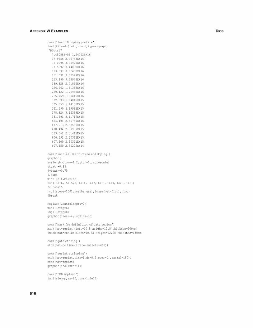
DIOSAPPENDIX W EXAMPLES
comm('load 1D doping profile')load(file=dc$init,noadd,type=xgraph) "BTotal" 7.45058E-06 1.24742E+16 37.9656 2.46743E+167 75.0995 3.39975E+16 77.5592 3.44030E+16 113.897 3.82438E+16 151.031 3.53599E+16 153.490 3.48948E+16 189.828 2.71856E+16 226.962 1.81358E+16 229.422 1.75968E+16 265.759 1.09415E+16 302.893 6.64015E+15 305.353 6.44130E+15 341.690 4.19992E+15 378.824 3.16369E+15 381.691 3.11717E+15 424.494 2.60759E+15 477.913 2.38589E+15 480.494 2.37937E+15 539.062 2.31412E+15 606.692 2.30362E+15 607.400 2.30351E+15 607.450 2.30272E+14
comm('initial 1D structure and doping')graphic(scale(ybottom=-1.2,ytop=1.,norescale)ytext=-0.85#ytext=-0.75!,nopnmin=-1e18,max=1e21zsc(-1e16,-5e15,0, 1e16, 1e17, 1e18, 1e19, 1e20, 1e21)!cut=1e15,col(steps=1001,nosubs,gas),logsw(net=flog),plot)!break
Replace(Control(ngra=2))mask:(step=6)impl:(step=8)graphic(clear=4,isoline=no)
comm('mask for definition of gate region')mask(mat=resist xleft=10.5 xright=12.5 thicknes=200nm)!mask(mat=resist xleft=10.75 xright=12.25 thicknes=130nm)
comm('gate etching')etch(mat=po time=1 rate(anisotr=460))
comm('resist stripping')etch(mat=resist,time=1,dt=0.2,over=0.,rat(a0=150))etch(mat=resist)graphic(isoline=fill)
comm('LDD implant')impl(elem=p,en=60,dose=1.3e13)
616
DIOS APPENDIX W EXAMPLES
graphic(isoline=no)
comm('deposition of spacer oxide')depo(mat=ox,thickness=200nm,amax=30)comm('spacer etching')etch(time=1 ra(mat=ox,aniso=230))graphic(isoline=fill)
comm('formation of protection oxide')diff( TEmperature=800 time=6 atmo=h2o2 vh2=1.67 cc(po=-3e20) Control(lprot=1))depo(ox,th=10nm)
comm('source/drain implant')impl(elem=as energy=80 dose=6e15)
comm('integral high temperature treatment')diff(TEmperature=950 time=15 Control(lprot=1))
! draw 2D picture comm()graphic(wait=0,plot,wait=1)
! draw 2D picture and 1D cross sectiongraph(win(top=10,lsh=3),xar(9,14),yar(-0.1,-0.1),star=boldtext(A B) xtext(9,13.85),ytext(-0.15,-0.15),clear=3,plot,next()xarr=default,ysect(-0.05),wait=0,cross,era(),wait=1)save(file=nmos1,type=mdraw)quit
617
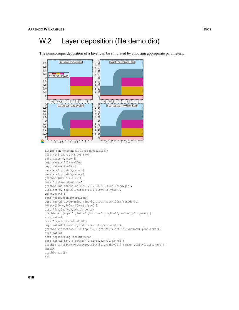
DIOSAPPENDIX W EXAMPLES
W.2 Layer deposition (file demo.dio)The nonisotropic deposition of a layer can be simulated by choosing appropriate parameters.
title('non homogeneous layer deposition')grid(x(-2.,2.),y(-2.,0),nx=4)subs(ysubs=0,ytop=3)depo:(amax=15,lmax=50nm)depo(mat=ox,th=40nm)mask(xl=0.,th=0.5,mat=ni)mask(xl=0.,th=0.5,mat=po)graphic:(win(zli=0.45))comm('initial structure')graphic(isoline=no,sc(xl=-1.,1.,-0.2,2.),col(subs,gas),win(left=0.,top=21.,bottom=10.1,right=15,ybox=1.),plot,next())comm('diffusion controlled')depo(mat=al,dtype=aniso,time=5.,growthrate=100nm/min,dt=0.1!dist=(100nm,200nm,500nm),fac=0.3)dist=70nm,fac=0.3,search=begin)graphic(win(top=10.,left=0.,bottom=0.,right=15,nombox),plot,next())etch(mat=al)comm('reaction controlled')depo(mat=al,time=5.,growthrate=100nm/min,dt=0.1)graphic(win(bottom=10.1,top=21.,right=29.7,left=15.1,nombox),plot,next())etch(mat=al)comm('sputtering, medium BIAS')depo(mat=al,th=0.6,rat(a0=70,a1=55,a2=-10,a3=-85))graphic(win(bottom=0,top=10,left=15.1,right=29.7,nombox),wait=0,plot,next())!breakgraphic(era())end
618
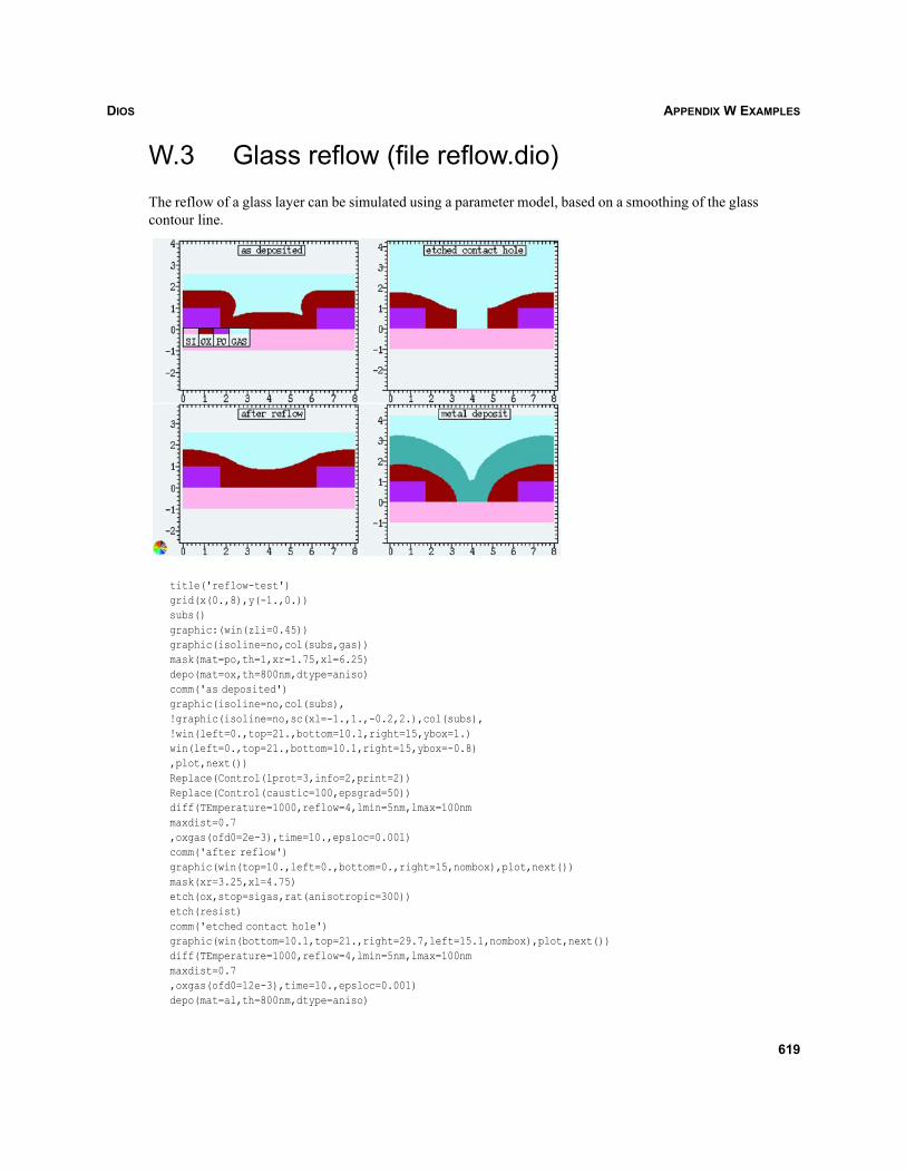
DIOS APPENDIX W EXAMPLES
W.3 Glass reflow (file reflow.dio)The reflow of a glass layer can be simulated using a parameter model, based on a smoothing of the glasscontour line.
title('reflow-test')grid(x(0.,8),y(-1.,0.))subs()graphic:(win(zli=0.45))graphic(isoline=no,col(subs,gas))mask(mat=po,th=1,xr=1.75,xl=6.25)depo(mat=ox,th=800nm,dtype=aniso)comm('as deposited')graphic(isoline=no,col(subs),!graphic(isoline=no,sc(xl=-1.,1.,-0.2,2.),col(subs),!win(left=0.,top=21.,bottom=10.1,right=15,ybox=1.)win(left=0.,top=21.,bottom=10.1,right=15,ybox=-0.8),plot,next())Replace(Control(lprot=3,info=2,print=2))Replace(Control(caustic=100,epsgrad=50))diff(TEmperature=1000,reflow=4,lmin=5nm,lmax=100nmmaxdist=0.7,oxgas(ofd0=2e-3),time=10.,epsloc=0.001)comm('after reflow')graphic(win(top=10.,left=0.,bottom=0.,right=15,nombox),plot,next())mask(xr=3.25,xl=4.75)etch(ox,stop=sigas,rat(anisotropic=300))etch(resist)comm('etched contact hole')graphic(win(bottom=10.1,top=21.,right=29.7,left=15.1,nombox),plot,next())diff(TEmperature=1000,reflow=4,lmin=5nm,lmax=100nmmaxdist=0.7,oxgas(ofd0=12e-3),time=10.,epsloc=0.001)depo(mat=al,th=800nm,dtype=aniso)
619

DIOSAPPENDIX W EXAMPLES
comm('metal deposit')depo(mat=al,th=0.6,rat(a0=70,a1=55,a2=-10,a3=-85))graphic(win(bottom=0,top=10,left=15.1,right=29.7,nombox),wait=0,plot,next())!breakgraphic(era())end
W.4 Layer system operations (file show.dio)This example demonstrates the complex interaction of deposition, mask, and etching operations for thesimulation of a contact structure.
title('contact')Replace(Control(maxtrl=2,autoada=-1))grid(xleft=-3,3,ybottom=-1,3.5,dx=.8)subs(ybottom=-1,ysubs=0,concentr=-1)depo:(lmin=1nm,lmax=50nm,amin=2,amax=10,dthick=10nm)etch:(lmin=1nm,lmax=50nm,amin=2,amax=10)#graphic(isoline=no,colors(subs=on),clear=4,col(mat(gas=7)))graphic(isoline=no,colors(subs=on,mat(gas=7)))Replace(Control(ngraphic=10,nsave=-1))
depo(mat=ox,thicknes=20nm)
mask(mat=ni,thicknes=0.15,xleft=-1) !.15 .015 .19 .25!diff:(lmax=20nm,lmin=5nm)
etch(time=10,ra(mat=si,a1=10),alpha(-55))diff(TEmperature=1000,time=165,
620
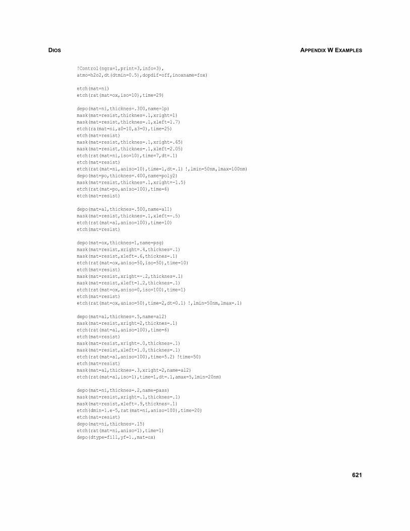
DIOS APPENDIX W EXAMPLES
!Control(ngra=1,print=3,info=3),atmo=h2o2,dt(dtmin=0.5),dopdif=off,inoxname=fox)
etch(mat=ni)etch(rat(mat=ox,iso=10),time=29)
depo(mat=ni,thicknes=.300,name=lp)mask(mat=resist,thicknes=.1,xright=1)mask(mat=resist,thicknes=.1,xleft=1.7)etch(ra(mat=ni,a0=10,a3=0),time=25)etch(mat=resist)mask(mat=resist,thicknes=.1,xright=.65)mask(mat=resist,thicknes=.1,xleft=2.05)etch(rat(mat=ni,iso=10),time=7,dt=.1)etch(mat=resist)etch(rat(mat=ni,aniso=10),time=1,dt=.1) !,lmin=50nm,lmax=100nm)depo(mat=po,thicknes=.400,name=poly2)mask(mat=resist,thicknes=.1,xright=-1.5)etch(rat(mat=po,aniso=100),time=6)etch(mat=resist)
depo(mat=al,thicknes=.500,name=al1)mask(mat=resist,thicknes=.1,xleft=-.5)etch(rat(mat=al,aniso=100),time=10)etch(mat=resist)
depo(mat=ox,thicknes=1,name=psg)mask(mat=resist,xright=.4,thicknes=.1)mask(mat=resist,xleft=.6,thicknes=.1)etch(rat(mat=ox,aniso=50,iso=50),time=10)etch(mat=resist)mask(mat=resist,xright=-.2,thicknes=.1)mask(mat=resist,xleft=1.2,thicknes=.1)etch(rat(mat=ox,aniso=0,iso=100),time=1)etch(mat=resist)etch(rat(mat=ox,aniso=50),time=2,dt=0.1) !,lmin=50nm,lmax=.1)
depo(mat=al,thicknes=.5,name=al2)mask(mat=resist,xright=2,thicknes=.1)etch(rat(mat=al,aniso=100),time=6)etch(mat=resist)mask(mat=resist,xright=.0,thicknes=.1)mask(mat=resist,xleft=1.0,thicknes=.1)etch(rat(mat=al,aniso=100),time=5.2) !time=50)etch(mat=resist)mask(mat=al,thicknes=.3,xright=2,name=al2)etch(rat(mat=al,iso=1),time=1,dt=.1,amax=5,lmin=20nm)
depo(mat=ni,thicknes=.2,name=pass)mask(mat=resist,xright=.1,thicknes=.1)mask(mat=resist,xleft=.9,thicknes=.1)etch(dmin=1.e-5,rat(mat=ni,aniso=100),time=20)etch(mat=resist)depo(mat=ni,thicknes=.15)etch(rat(mat=ni,aniso=1),time=1)depo(dtype=fill,yf=1.,mat=ox)
621
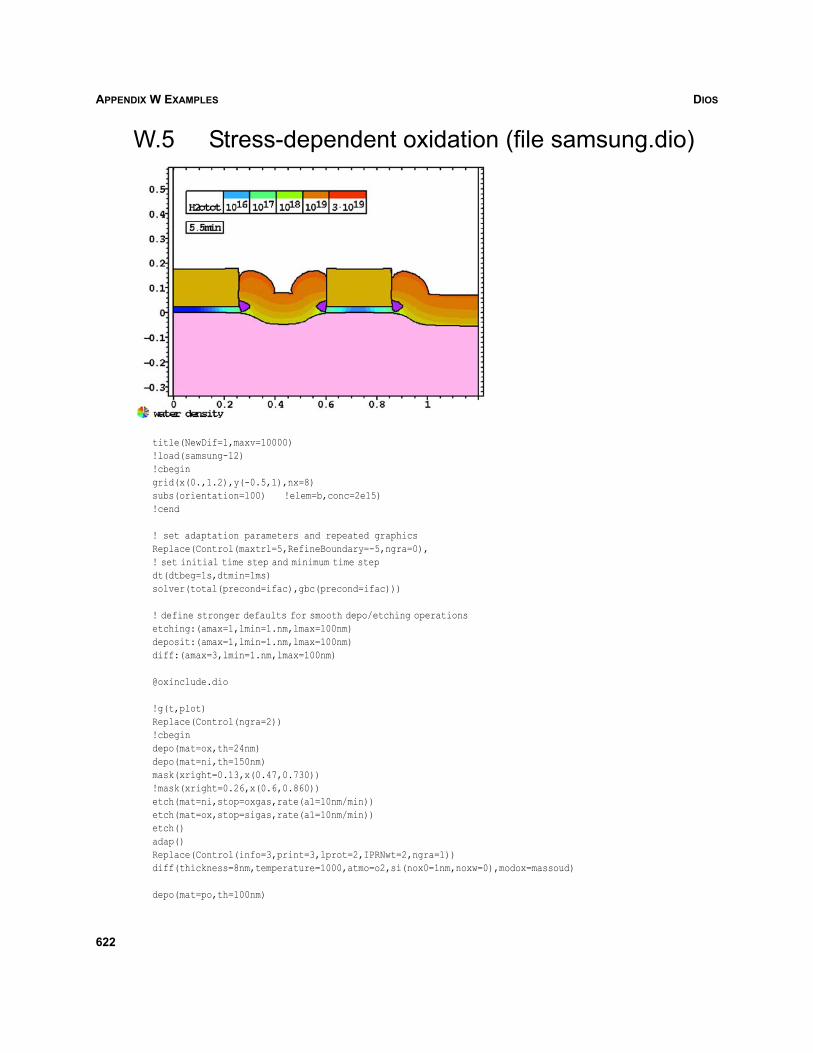
DIOSAPPENDIX W EXAMPLES
W.5 Stress-dependent oxidation (file samsung.dio)
title(NewDif=1,maxv=10000)!load(samsung-12)!cbegingrid(x(0.,1.2),y(-0.5,1),nx=8)subs(orientation=100) !elem=b,conc=2e15)!cend
! set adaptation parameters and repeated graphics Replace(Control(maxtrl=5,RefineBoundary=-5,ngra=0),! set initial time step and minimum time stepdt(dtbeg=1s,dtmin=1ms)solver(total(precond=ifac),gbc(precond=ifac)))
! define stronger defaults for smooth depo/etching operationsetching:(amax=1,lmin=1.nm,lmax=100nm)deposit:(amax=1,lmin=1.nm,lmax=100nm)diff:(amax=3,lmin=1.nm,lmax=100nm)
@oxinclude.dio
!g(t,plot)Replace(Control(ngra=2))!cbegindepo(mat=ox,th=24nm)depo(mat=ni,th=150nm)mask(xright=0.13,x(0.47,0.730))!mask(xright=0.26,x(0.6,0.860))etch(mat=ni,stop=oxgas,rate(a1=10nm/min))etch(mat=ox,stop=sigas,rate(a1=10nm/min))etch()adap()Replace(Control(info=3,print=3,lprot=2,IPRNwt=2,ngra=1))diff(thickness=8nm,temperature=1000,atmo=o2,si(nox0=1nm,noxw=0),modox=massoud)
depo(mat=po,th=100nm)
622
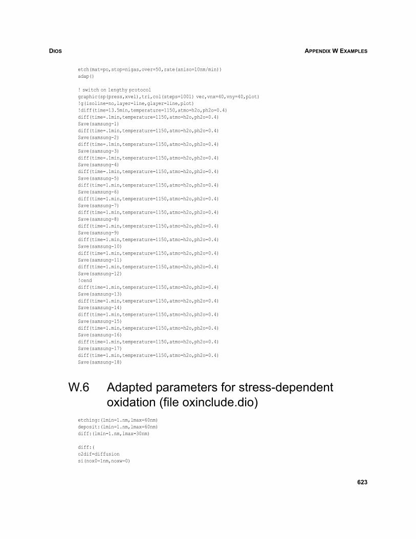
DIOS APPENDIX W EXAMPLES
etch(mat=po,stop=nigas,over=50,rate(aniso=10nm/min))adap()
! switch on lengthy protocolgraphic(sp(press,xvel),tri,col(steps=1001) vec,vnx=40,vny=40,plot)!g(isoline=no,layer=line,glayer=line,plot)!diff(time=13.5min,temperature=1150,atmo=h2o,ph2o=0.4)diff(time=.1min,temperature=1150,atmo=h2o,ph2o=0.4)Save(samsung-1)diff(time=.1min,temperature=1150,atmo=h2o,ph2o=0.4)Save(samsung-2)diff(time=.1min,temperature=1150,atmo=h2o,ph2o=0.4)Save(samsung-3)diff(time=.1min,temperature=1150,atmo=h2o,ph2o=0.4)Save(samsung-4)diff(time=.1min,temperature=1150,atmo=h2o,ph2o=0.4)Save(samsung-5)diff(time=1.min,temperature=1150,atmo=h2o,ph2o=0.4)Save(samsung-6)diff(time=1.min,temperature=1150,atmo=h2o,ph2o=0.4)Save(samsung-7)diff(time=1.min,temperature=1150,atmo=h2o,ph2o=0.4)Save(samsung-8)diff(time=1.min,temperature=1150,atmo=h2o,ph2o=0.4)Save(samsung-9)diff(time=1.min,temperature=1150,atmo=h2o,ph2o=0.4)Save(samsung-10)diff(time=1.min,temperature=1150,atmo=h2o,ph2o=0.4)Save(samsung-11)diff(time=1.min,temperature=1150,atmo=h2o,ph2o=0.4)Save(samsung-12)!cenddiff(time=1.min,temperature=1150,atmo=h2o,ph2o=0.4)Save(samsung-13)diff(time=1.min,temperature=1150,atmo=h2o,ph2o=0.4)Save(samsung-14)diff(time=1.min,temperature=1150,atmo=h2o,ph2o=0.4)Save(samsung-15)diff(time=1.min,temperature=1150,atmo=h2o,ph2o=0.4)Save(samsung-16)diff(time=1.min,temperature=1150,atmo=h2o,ph2o=0.4)Save(samsung-17)diff(time=1.min,temperature=1150,atmo=h2o,ph2o=0.4)Save(samsung-18)
W.6 Adapted parameters for stress-dependent oxidation (file oxinclude.dio)
etching:(lmin=1.nm,lmax=60nm)deposit:(lmin=1.nm,lmax=60nm)diff:(lmin=1.nm,lmax=30nm)
diff:(o2dif=diffusionsi(nox0=1nm,noxw=0)
623
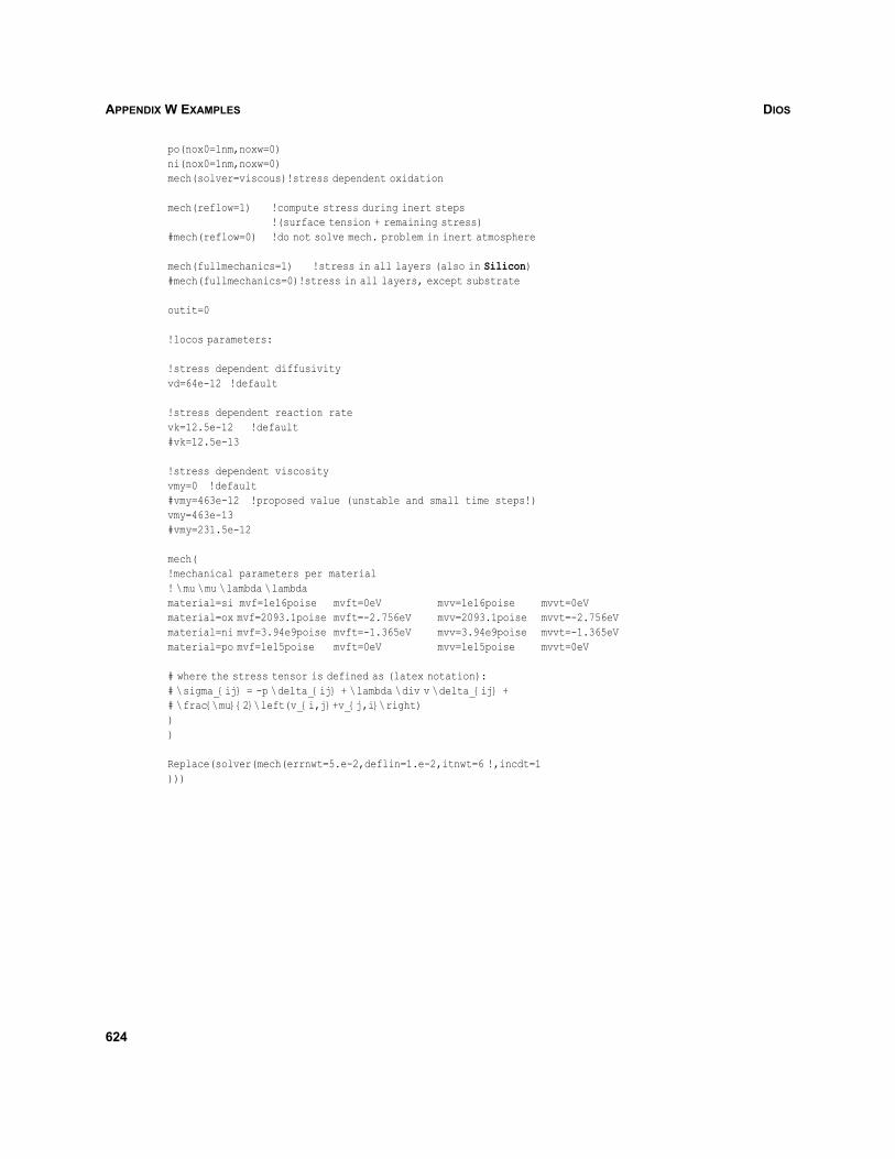
DIOSAPPENDIX W EXAMPLES
po(nox0=1nm,noxw=0)ni(nox0=1nm,noxw=0)mech(solver=viscous)!stress dependent oxidation
mech(reflow=1) !compute stress during inert steps !(surface tension + remaining stress)#mech(reflow=0) !do not solve mech. problem in inert atmosphere
mech(fullmechanics=1) !stress in all layers (also in Silicon)#mech(fullmechanics=0)!stress in all layers, except substrate
outit=0
!locos parameters:
!stress dependent diffusivity vd=64e-12 !default
!stress dependent reaction rate vk=12.5e-12 !default#vk=12.5e-13
!stress dependent viscosity vmy=0 !default#vmy=463e-12 !proposed value (unstable and small time steps!)vmy=463e-13#vmy=231.5e-12
mech(!mechanical parameters per material ! \mu \mu \lambda \lambdamaterial=si mvf=1e16poise mvft=0eV mvv=1e16poise mvvt=0eVmaterial=ox mvf=2093.1poise mvft=-2.756eV mvv=2093.1poise mvvt=-2.756eVmaterial=ni mvf=3.94e9poise mvft=-1.365eV mvv=3.94e9poise mvvt=-1.365eVmaterial=po mvf=1e15poise mvft=0eV mvv=1e15poise mvvt=0eV
# where the stress tensor is defined as (latex notation):# \sigma_{ij} = -p \delta_{ij} + \lambda \div v \delta_{ij} +# \frac{\mu}{2}\left(v_{i,j}+v_{j,i}\right)))
Replace(solver(mech(errnwt=5.e-2,deflin=1.e-2,itnwt=6 !,incdt=1)))
624
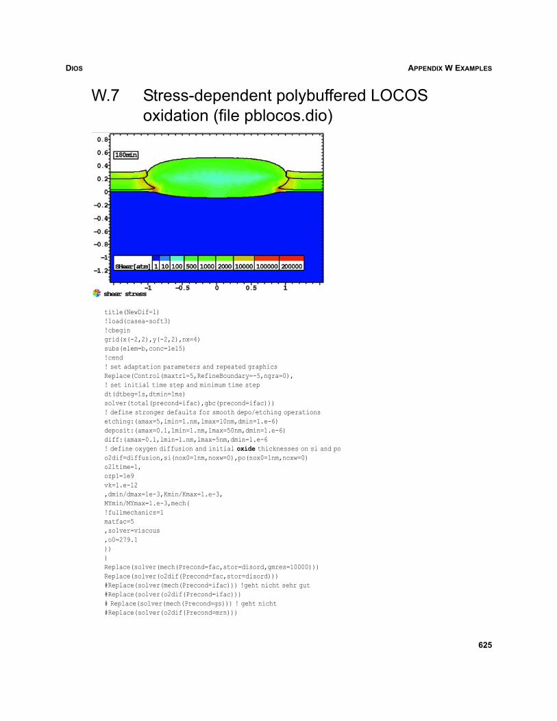
DIOS APPENDIX W EXAMPLES
W.7 Stress-dependent polybuffered LOCOS oxidation (file pblocos.dio)
title(NewDif=1)!load(casea-soft3)!cbegingrid(x(-2,2),y(-2,2),nx=4)subs(elem=b,conc=1e15)!cend! set adaptation parameters and repeated graphicsReplace(Control(maxtrl=5,RefineBoundary=-5,ngra=0),! set initial time step and minimum time stepdt(dtbeg=1s,dtmin=1ms)solver(total(precond=ifac),gbc(precond=ifac)))! define stronger defaults for smooth depo/etching operationsetching:(amax=5,lmin=1.nm,lmax=10nm,dmin=1.e-6)deposit:(amax=0.1,lmin=1.nm,lmax=50nm,dmin=1.e-6)diff:(amax=0.1,lmin=1.nm,lmax=5nm,dmin=1.e-6! define oxygen diffusion and initial oxide thicknesses on si and poo2dif=diffusion,si(nox0=1nm,noxw=0),po(nox0=1nm,noxw=0)o2ltime=1,ozp1=1e9vk=1.e-12,dmin/dmax=1e-3,Kmin/Kmax=1.e-3,MYmin/MYmax=1.e-3,mech(!fullmechanics=1matfac=5,solver=viscous,o0=279.1)))Replace(solver(mech(Precond=fac,stor=disord,gmres=10000)))Replace(solver(o2dif(Precond=fac,stor=disord)))#Replace(solver(mech(Precond=ifac))) !geht nicht sehr gut#Replace(solver(o2dif(Precond=ifac)))# Replace(solver(mech(Precond=gs))) ! geht nicht#Replace(solver(o2dif(Precond=mrn)))
625
DIOSAPPENDIX W EXAMPLES
!cbegindepo(ox,th=270A)!depo(ox,th=700A)depo(po,th=1700A)!depo(po,th=2300A)mask(ni,th=1000A,x(,-1,1))!cend
graphic(sp(h2o,xvel),col(steps=1001),tri,vec,vnx=40,vny=40,plot)Replace(Control(lprot=2,IPRNwt=2,ngra=2))!cbegin!trace(traceon,tp)Replace(var(spec=h2o,print=2,spec=pres,print=2,spec=rho,print=2))!diff(temperature=950,atmo=h2o2,thickness=8200A)!cbegin! time=313Replace(Control(nsave=10000))diff(temperature=950,atmo=h2o2,time=1)diff(temperature=950,atmo=h2o2,time=4) !5diff(temperature=950,atmo=h2o2,time=5) !10diff(temperature=950,atmo=h2o2,time=10) !20diff(temperature=950,atmo=h2o2,time=10) !30diff(temperature=950,atmo=h2o2,time=10) !40diff(temperature=950,atmo=h2o2,time=10) !50diff(temperature=950,atmo=h2o2,time=10) !60diff(temperature=950,atmo=h2o2,time=10) !70diff(temperature=950,atmo=h2o2,time=10) !80diff(temperature=950,atmo=h2o2,time=10) !90diff(temperature=950,atmo=h2o2,time=10) !100diff(temperature=950,atmo=h2o2,time=20) !120diff(temperature=950,atmo=h2o2,time=20) !140diff(temperature=950,atmo=h2o2,time=20) !160diff(temperature=950,atmo=h2o2,time=20) !180diff(temperature=950,atmo=h2o2,time=20) !200diff(temperature=950,atmo=h2o2,time=20) !220diff(temperature=950,atmo=h2o2,time=20) !240diff(temperature=950,atmo=h2o2,time=20) !260diff(temperature=950,atmo=h2o2,time=20) !280diff(temperature=950,atmo=h2o2,time=20) !300diff(temperature=950,atmo=h2o2,time=13) !313
W.8 Variety of oxidation structures using the parameter model (file oxidall.dio)
! Examples file for simulation of (some) oxidation structures !!!title('oxidation of n+ doped si') Replace(Control(maxtrl=4,ngra=1))grid(x(-2.,2),y(-2.,0),nx=4)subs()graphic(
626
DIOS APPENDIX W EXAMPLES
!scale(ybottom=-4,ytop=3,norescale)colors(mat(gas=7)),clear=3,plot,clear=4)depo(ox,th=20nm)mask(xleft=0.)impl(elem=as,dose=6e15,en=80)etch(resist)diff(temperature=1000,atmo=o2,time=40contr(ngra=1))graphic(wait=0,plot,wait=1)!!!!!reset()title('poly spacer')Replace(Control(maxtrl=2,dopada=0,ngra=1))grid(x(-2.,3),y(-2.,0),nx=4)subs()graphic(isoline=no,colors(subs),!scale(ybottom=-4,ytop=3,norescale),colors(mat(gas=7)),clear=3,plot,clear=4)depo(ox,th=16nm)depo(mat=po,thicknes=500nm,conc(pTotal=3e20))diff(TEmperature=975 time=53 atmo=o2 po2=1)mask(xright=1)etch(time=1 rate(mat=ox aniso=70))etch(time=1 rate(mat=po aniso=500))etch(mat=resist)
etch(time=1 rate(mat=ox aniso=70))etch(time=1 rate(mat=ox aniso=70))diff(TEmperature=950 time=63 atmo=o2 po2=1contr(ngra=1))depo(mat=po,thicknes=500nm)mask(xright=-1)etch(time=1 rate(mat=po aniso=510)) ! mit Fadenstopetch(mat=resist)etch(time=1 rate(mat=ox aniso=60))diff(TEmperature=950 time=14 atmo=h2o2 vh2=1.6contr(lprot=2,info=2,print=2)contr(ngra=1))graphic(wait=0,plot,wait=1)!!reset()title('birds head')Replace(Control(maxtrl=4,dopada=0,ngra=1))grid(x(-2.,2),y(-2.,0),nx=4)subs()graphic(isoline=no,colors(subs),!scale(ybottom=-4,ytop=3,norescale),colors(mat(gas=7)),clear=3,plot,clear=4)depo(ox,th=20nm)
627
DIOSAPPENDIX W EXAMPLES
depo(ni,th=130nm)mask(xleft=0.)etch(ni,stop=oxgas,rat(a0=100))etch(resist)etch(ox,stop=sigas,rat(a0=100))etch(si,remove=60nm,rat(a1=100,a3=-80))diff(temperature=1000,atmo=h2o2,time=150contr(ngra=1))graphic(wait=0,plot,wait=1)!!etch(mat=ni)etch(mat=ox,remove=100nm)comm('sacrificial oxide')diff(TEmperature=1000,time=95,atmo=hcl,cl=3contr(ngra=1))graphic(wait=0,plot,wait=1)!!!reset()title('planar oxide')Replace(Control(maxtrl=2,dopada=0,ngra=1))grid(x(-2.,2),y(-2.,0),nx=4)subs()graphic(isoline=no,colors(subs),!scale(ybottom=-4,ytop=3,norescale),colors(mat(gas=7)),clear=3,plot,clear=4)mask(ni,xleft=-1.,xright=1)etch(si,remo=200nm)!g(scale(-0.8,0.,4,eq))diff(TEmperature=1000,time=100,atmo=h2o2,vh2=1.67contr(lprot=2,info=2,print=2)contr(ngra=1))etch(ni)graphic(wait=0,plot,wait=1)!!!reset()title('mesa structure')Replace(Control(maxtrl=2,dopada=0,ngra=1))grid(x(-2.,2),y(-2.,0),nx=4)subs()graphic(isoline=no,colors(subs),!scale(ybottom=-4,ytop=3,norescale),colors(mat(gas=7)),clear=3,plot,clear=4)mask(ni,xleft=-1.,xright=1)etch(si,remo=500nm)diff(TEmperature=1000,time=100,atmo=h2o2,vh2=1.67contr(lprot=2,info=2,print=2)contr(ngra=1))etch(ni)graphic(wait=0,plot,wait=1)
628
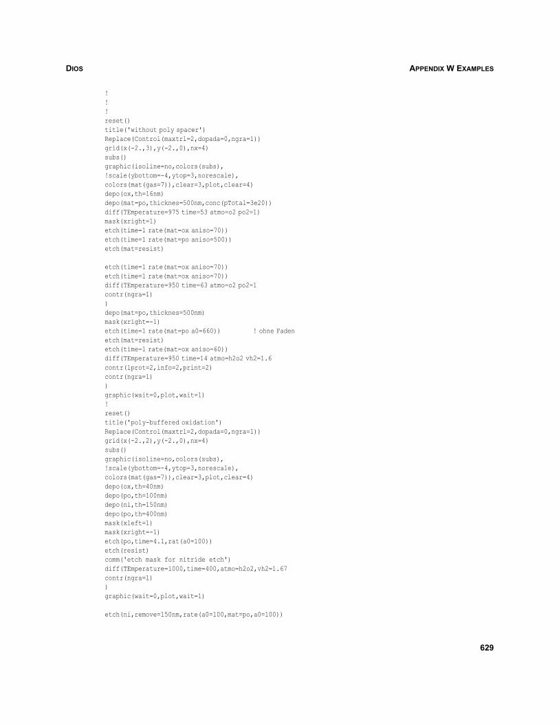
DIOS APPENDIX W EXAMPLES
!!!reset()title('without poly spacer')Replace(Control(maxtrl=2,dopada=0,ngra=1))grid(x(-2.,3),y(-2.,0),nx=4)subs()graphic(isoline=no,colors(subs),!scale(ybottom=-4,ytop=3,norescale),colors(mat(gas=7)),clear=3,plot,clear=4)depo(ox,th=16nm)depo(mat=po,thicknes=500nm,conc(pTotal=3e20))diff(TEmperature=975 time=53 atmo=o2 po2=1)mask(xright=1)etch(time=1 rate(mat=ox aniso=70))etch(time=1 rate(mat=po aniso=500))etch(mat=resist)
etch(time=1 rate(mat=ox aniso=70))etch(time=1 rate(mat=ox aniso=70))diff(TEmperature=950 time=63 atmo=o2 po2=1contr(ngra=1))depo(mat=po,thicknes=500nm)mask(xright=-1)etch(time=1 rate(mat=po a0=660)) ! ohne Fadenetch(mat=resist)etch(time=1 rate(mat=ox aniso=60))diff(TEmperature=950 time=14 atmo=h2o2 vh2=1.6contr(lprot=2,info=2,print=2)contr(ngra=1))graphic(wait=0,plot,wait=1)!reset()title('poly-buffered oxidation')Replace(Control(maxtrl=2,dopada=0,ngra=1))grid(x(-2.,2),y(-2.,0),nx=4)subs()graphic(isoline=no,colors(subs),!scale(ybottom=-4,ytop=3,norescale),colors(mat(gas=7)),clear=3,plot,clear=4)depo(ox,th=40nm)depo(po,th=100nm)depo(ni,th=150nm)depo(po,th=400nm)mask(xleft=1)mask(xright=-1)etch(po,time=4.1,rat(a0=100))etch(resist)comm('etch mask for nitride etch') diff(TEmperature=1000,time=400,atmo=h2o2,vh2=1.67contr(ngra=1))graphic(wait=0,plot,wait=1)
etch(ni,remove=150nm,rate(a0=100,mat=po,a0=100))
629
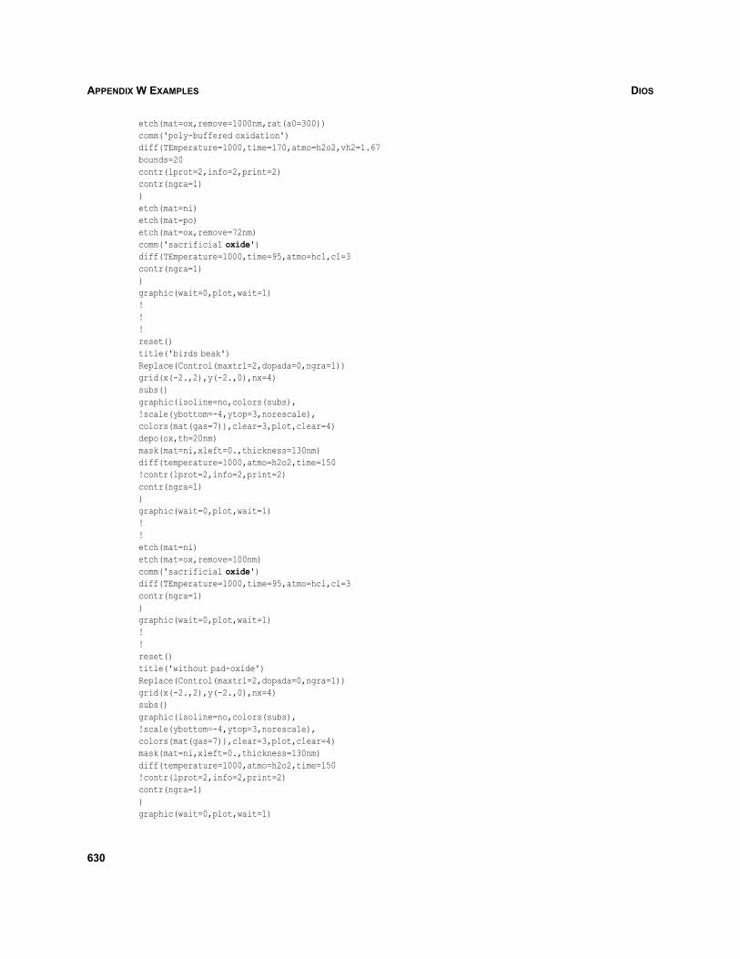
DIOSAPPENDIX W EXAMPLES
etch(mat=ox,remove=1000nm,rat(a0=300))comm('poly-buffered oxidation')diff(TEmperature=1000,time=170,atmo=h2o2,vh2=1.67bounds=20contr(lprot=2,info=2,print=2)contr(ngra=1))etch(mat=ni)etch(mat=po)etch(mat=ox,remove=72nm)comm('sacrificial oxide')diff(TEmperature=1000,time=95,atmo=hcl,cl=3contr(ngra=1))graphic(wait=0,plot,wait=1)!!!reset()title('birds beak')Replace(Control(maxtrl=2,dopada=0,ngra=1))grid(x(-2.,2),y(-2.,0),nx=4)subs()graphic(isoline=no,colors(subs),!scale(ybottom=-4,ytop=3,norescale),colors(mat(gas=7)),clear=3,plot,clear=4)depo(ox,th=20nm)mask(mat=ni,xleft=0.,thickness=130nm)diff(temperature=1000,atmo=h2o2,time=150!contr(lprot=2,info=2,print=2)contr(ngra=1))graphic(wait=0,plot,wait=1)!!etch(mat=ni)etch(mat=ox,remove=100nm)comm('sacrificial oxide')diff(TEmperature=1000,time=95,atmo=hcl,cl=3contr(ngra=1))graphic(wait=0,plot,wait=1)!!reset()title('without pad-oxide')Replace(Control(maxtrl=2,dopada=0,ngra=1))grid(x(-2.,2),y(-2.,0),nx=4)subs()graphic(isoline=no,colors(subs),!scale(ybottom=-4,ytop=3,norescale),colors(mat(gas=7)),clear=3,plot,clear=4)mask(mat=ni,xleft=0.,thickness=130nm)diff(temperature=1000,atmo=h2o2,time=150!contr(lprot=2,info=2,print=2)contr(ngra=1))graphic(wait=0,plot,wait=1)
630
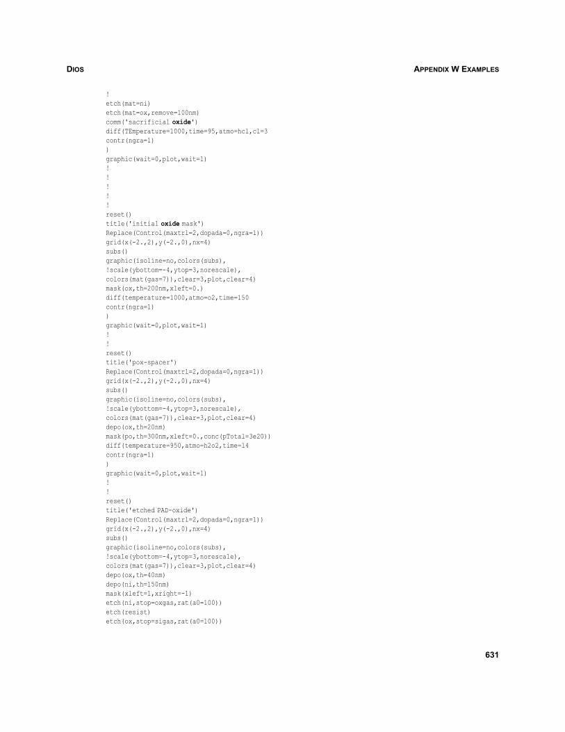
DIOS APPENDIX W EXAMPLES
!etch(mat=ni)etch(mat=ox,remove=100nm)comm('sacrificial oxide')diff(TEmperature=1000,time=95,atmo=hcl,cl=3contr(ngra=1))graphic(wait=0,plot,wait=1)!!!!!reset()title('initial oxide mask')Replace(Control(maxtrl=2,dopada=0,ngra=1))grid(x(-2.,2),y(-2.,0),nx=4)subs()graphic(isoline=no,colors(subs),!scale(ybottom=-4,ytop=3,norescale),colors(mat(gas=7)),clear=3,plot,clear=4)mask(ox,th=200nm,xleft=0.)diff(temperature=1000,atmo=o2,time=150contr(ngra=1))graphic(wait=0,plot,wait=1)!!reset()title('pox-spacer')Replace(Control(maxtrl=2,dopada=0,ngra=1))grid(x(-2.,2),y(-2.,0),nx=4)subs()graphic(isoline=no,colors(subs),!scale(ybottom=-4,ytop=3,norescale),colors(mat(gas=7)),clear=3,plot,clear=4)depo(ox,th=20nm)mask(po,th=300nm,xleft=0.,conc(pTotal=3e20))diff(temperature=950,atmo=h2o2,time=14contr(ngra=1))graphic(wait=0,plot,wait=1)!!reset()title('etched PAD-oxide')Replace(Control(maxtrl=2,dopada=0,ngra=1))grid(x(-2.,2),y(-2.,0),nx=4)subs()graphic(isoline=no,colors(subs),!scale(ybottom=-4,ytop=3,norescale),colors(mat(gas=7)),clear=3,plot,clear=4)depo(ox,th=40nm)depo(ni,th=150nm)mask(xleft=1,xright=-1)etch(ni,stop=oxgas,rat(a0=100))etch(resist)etch(ox,stop=sigas,rat(a0=100))
631
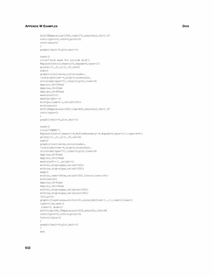
DIOSAPPENDIX W EXAMPLES
diff(TEmperature=1000,time=170,atmo=h2o2,vh2=1.67contr(lprot=2,info=2,print=2)contr(ngra=1))graphic(wait=0,plot,wait=1)
reset()title('etch mask for nitride etch') Replace(Control(maxtrl=2,dopada=0,ngra=1))grid(x(-2.,2),y(-2.,0),nx=4)subs()graphic(isoline=no,colors(subs),!scale(ybottom=-4,ytop=3,norescale),colors(mat(gas=7)),clear=3,plot,clear=4)depo(ni,th=150nm)depo(ox,th=20nm)depo(po,th=400nm)mask(xleft=1)mask(xright=-1)etch(po,time=4.1,rat(a0=100))etch(resist)diff(TEmperature=1000,time=400,atmo=h2o2,vh2=1.67contr(ngra=1))graphic(wait=0,plot,wait=1)
reset()title('SWAMI')Replace(Control(maxtrl=4,RefineBoundary=-4,dopada=0,ngra=1))!,ipgrid=4))grid(x(-2.,2),y(-2.,0),nx=16)subs()graphic(isoline=no,colors(subs),!scale(ybottom=-4,ytop=3,norescale),colors(mat(gas=7)),clear=3,plot,clear=4)depo(ox,th=45nm)depo(ni,th=150nm)mask(xleft=-1.,xright=1)etch(ni,stop=oxgas,rat(a0=100))etch(ox,stop=sigas,rat(a0=100))adap()etch(si,remo=300nm,rat(a0=100),Control(retri=4))etch(resist)depo(ox,th=45nm)depo(ni,th=150nm)etch(ni,stop=oxgas,rat(aniso=100))etch(ox,stop=sigas,rat(aniso=100))!g(t,plot)graphic(layer=area,win(to=10),scale(ybottom=-1.,1.),next()clear=1 layer=line,next() clear=3, draw())diff(time=260,TEmperature=1024,atmo=h2o,th2o=80contr(lprot=2,info=2,print=2)Control(ngra=1))graphic(wait=0,plot,wait=1)!end
632
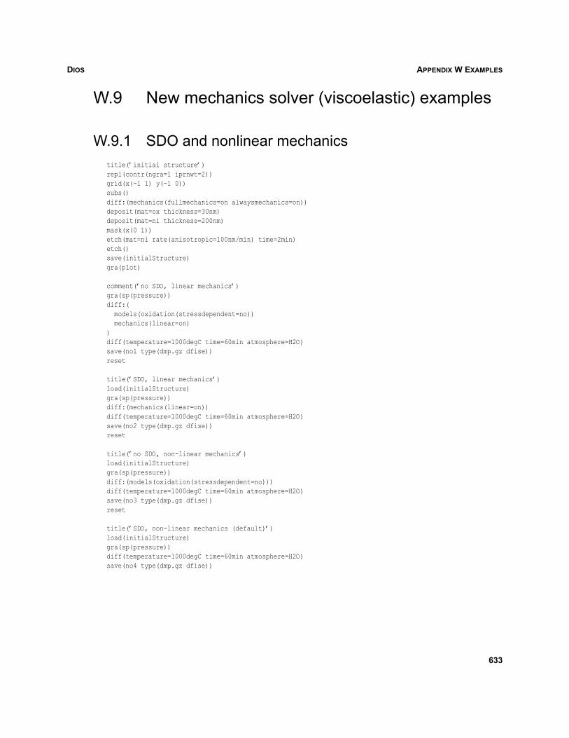
DIOS APPENDIX W EXAMPLES
W.9 New mechanics solver (viscoelastic) examples
W.9.1 SDO and nonlinear mechanicstitle(’initial structure’)repl(contr(ngra=1 iprnwt=2))grid(x(-1 1) y(-1 0))subs()diff:(mechanics(fullmechanics=on alwaysmechanics=on))deposit(mat=ox thickness=30nm)deposit(mat=ni thickness=200nm)mask(x(0 1))etch(mat=ni rate(anisotropic=100nm/min) time=2min)etch()save(initialStructure)gra(plot)
comment(’no SDO, linear mechanics’)gra(sp(pressure))diff:( models(oxidation(stressdependent=no)) mechanics(linear=on))diff(temperature=1000degC time=60min atmosphere=H2O)save(no1 type(dmp.gz dfise))reset
title(’SDO, linear mechanics’)load(initialStructure)gra(sp(pressure))diff:(mechanics(linear=on))diff(temperature=1000degC time=60min atmosphere=H2O)save(no2 type(dmp.gz dfise))reset
title(’no SDO, non-linear mechanics’)load(initialStructure)gra(sp(pressure))diff:(models(oxidation(stressdependent=no)))diff(temperature=1000degC time=60min atmosphere=H2O)save(no3 type(dmp.gz dfise))reset
title(’SDO, non-linear mechanics (default)’)load(initialStructure)gra(sp(pressure))diff(temperature=1000degC time=60min atmosphere=H2O)save(no4 type(dmp.gz dfise))
633
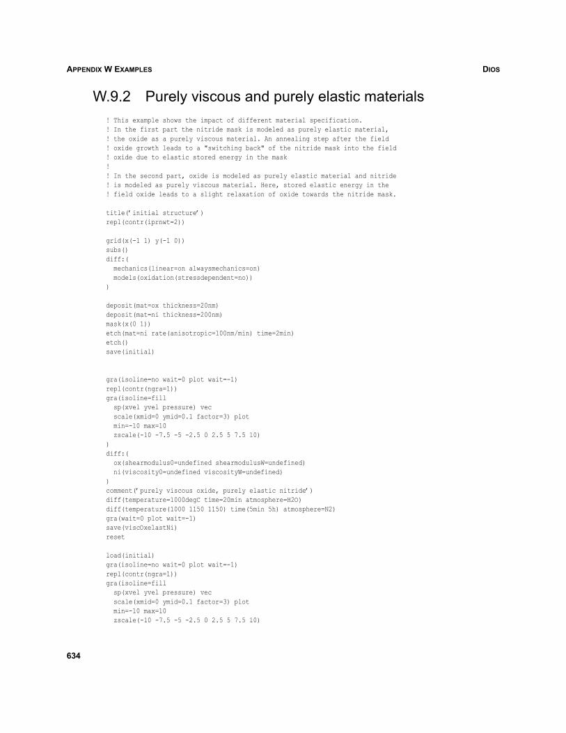
DIOSAPPENDIX W EXAMPLES
W.9.2 Purely viscous and purely elastic materials! This example shows the impact of different material specification.! In the first part the nitride mask is modeled as purely elastic material,! the oxide as a purely viscous material. An annealing step after the field! oxide growth leads to a "switching back" of the nitride mask into the field! oxide due to elastic stored energy in the mask!! In the second part, oxide is modeled as purely elastic material and nitride! is modeled as purely viscous material. Here, stored elastic energy in the ! field oxide leads to a slight relaxation of oxide towards the nitride mask.
title(’initial structure’)repl(contr(iprnwt=2))
grid(x(-1 1) y(-1 0))subs()diff:( mechanics(linear=on alwaysmechanics=on) models(oxidation(stressdependent=no)))
deposit(mat=ox thickness=20nm)deposit(mat=ni thickness=200nm)mask(x(0 1))etch(mat=ni rate(anisotropic=100nm/min) time=2min)etch()save(initial)
gra(isoline=no wait=0 plot wait=-1)repl(contr(ngra=1))gra(isoline=fill sp(xvel yvel pressure) vec scale(xmid=0 ymid=0.1 factor=3) plot min=-10 max=10 zscale(-10 -7.5 -5 -2.5 0 2.5 5 7.5 10))diff:( ox(shearmodulus0=undefined shearmodulusW=undefined) ni(viscosity0=undefined viscosityW=undefined))comment(’purely viscous oxide, purely elastic nitride’)diff(temperature=1000degC time=20min atmosphere=H2O)diff(temperature(1000 1150 1150) time(5min 5h) atmosphere=N2)gra(wait=0 plot wait=-1)save(viscOxelastNi)reset
load(initial)gra(isoline=no wait=0 plot wait=-1)repl(contr(ngra=1))gra(isoline=fill sp(xvel yvel pressure) vec scale(xmid=0 ymid=0.1 factor=3) plot min=-10 max=10 zscale(-10 -7.5 -5 -2.5 0 2.5 5 7.5 10)
634
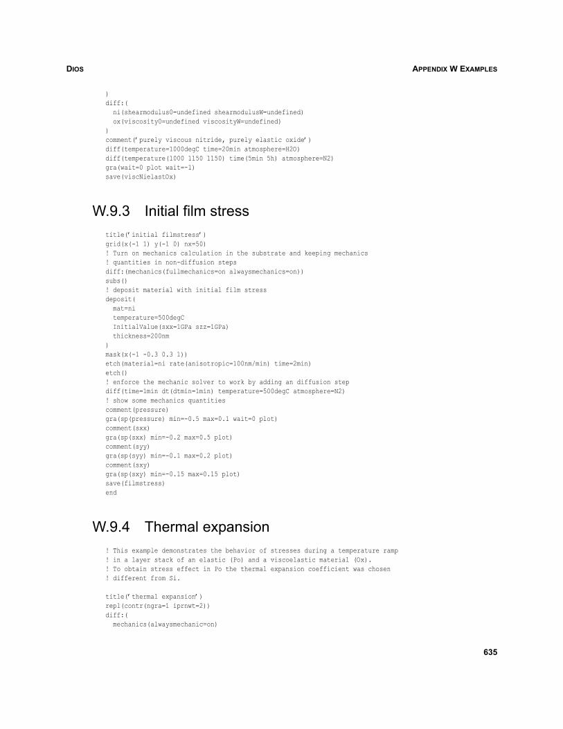
DIOS APPENDIX W EXAMPLES
)diff:( ni(shearmodulus0=undefined shearmodulusW=undefined) ox(viscosity0=undefined viscosityW=undefined))comment(’purely viscous nitride, purely elastic oxide’)diff(temperature=1000degC time=20min atmosphere=H2O)diff(temperature(1000 1150 1150) time(5min 5h) atmosphere=N2)gra(wait=0 plot wait=-1)save(viscNielastOx)
W.9.3 Initial film stresstitle(’initial filmstress’)grid(x(-1 1) y(-1 0) nx=50)! Turn on mechanics calculation in the substrate and keeping mechanics! quantities in non-diffusion stepsdiff:(mechanics(fullmechanics=on alwaysmechanics=on))subs()! deposit material with initial film stressdeposit( mat=ni temperature=500degC InitialValue(sxx=1GPa szz=1GPa) thickness=200nm)mask(x(-1 -0.3 0.3 1))etch(material=ni rate(anisotropic=100nm/min) time=2min)etch()! enforce the mechanic solver to work by adding an diffusion stepdiff(time=1min dt(dtmin=1min) temperature=500degC atmosphere=N2)! show some mechanics quantitiescomment(pressure)gra(sp(pressure) min=-0.5 max=0.1 wait=0 plot)comment(sxx)gra(sp(sxx) min=-0.2 max=0.5 plot)comment(syy)gra(sp(syy) min=-0.1 max=0.2 plot)comment(sxy)gra(sp(sxy) min=-0.15 max=0.15 plot)save(filmstress)end
W.9.4 Thermal expansion! This example demonstrates the behavior of stresses during a temperature ramp! in a layer stack of an elastic (Po) and a viscoelastic material (Ox).! To obtain stress effect in Po the thermal expansion coefficient was chosen! different from Si.
title(’thermal expansion’)repl(contr(ngra=1 iprnwt=2))diff:( mechanics(alwaysmechanic=on)
635
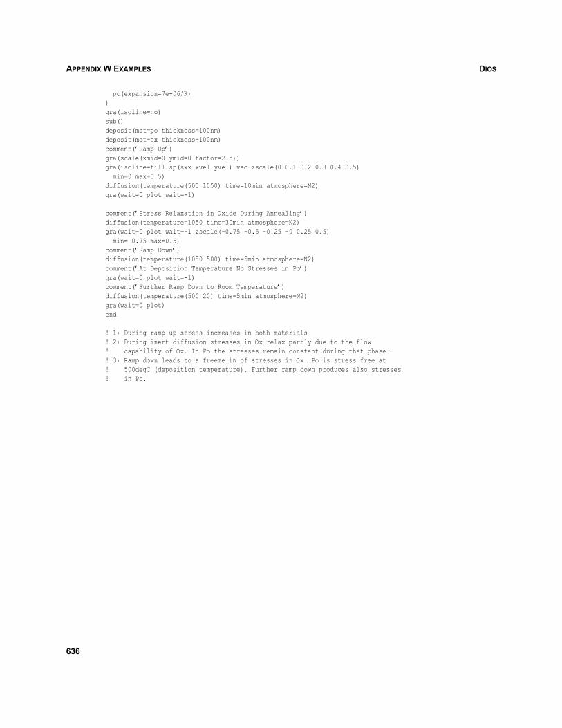
DIOSAPPENDIX W EXAMPLES
po(expansion=7e-06/K))gra(isoline=no)sub()deposit(mat=po thickness=100nm)deposit(mat=ox thickness=100nm)comment(’Ramp Up’)gra(scale(xmid=0 ymid=0 factor=2.5))gra(isoline=fill sp(sxx xvel yvel) vec zscale(0 0.1 0.2 0.3 0.4 0.5) min=0 max=0.5)diffusion(temperature(500 1050) time=10min atmosphere=N2)gra(wait=0 plot wait=-1)
comment(’Stress Relaxation in Oxide During Annealing’)diffusion(temperature=1050 time=30min atmosphere=N2)gra(wait=0 plot wait=-1 zscale(-0.75 -0.5 -0.25 -0 0.25 0.5) min=-0.75 max=0.5)comment(’Ramp Down’)diffusion(temperature(1050 500) time=5min atmosphere=N2)comment(’At Deposition Temperature No Stresses in Po’)gra(wait=0 plot wait=-1)comment(’Further Ramp Down to Room Temperature’)diffusion(temperature(500 20) time=5min atmosphere=N2)gra(wait=0 plot)end
! 1) During ramp up stress increases in both materials! 2) During inert diffusion stresses in Ox relax partly due to the flow! capability of Ox. In Po the stresses remain constant during that phase.! 3) Ramp down leads to a freeze in of stresses in Ox. Po is stress free at! 500degC (deposition temperature). Further ramp down produces also stresses! in Po.
636
DIOS BIBLIOGRAPHY
Dios
Bibliography
[1] G. K. Ackermann and E. Ebert, “Autodoping Phenomena in Epitaxial Silicon,” Journal of theElectrochemical Society, vol. 130, no. 9, pp. 1910–1915, 1983.
[2] D. H. Ahn et al., “A Highly Practical Modified LOCOS Isolation Technology for the 256 MbitDRAM,” in IEDM Technical Digest, San Francisco, CA, USA, pp. 679–682, December 1994.
[3] D. A. Antoniadis, A. G. Gonzalez, and R. W. Dutton, “Boron in Near-Intrinsic <100> and <111>Silicon under Inert and Oxidizing Ambients—Diffusion and Segregation,” Journal of theElectrochemical Society, vol. 125, no. 5, pp. 813–819, 1978.
[4] R. E. Bank, PLTMG: A Software Package for Solving Elliptic Partial Differential Equations, Users’Guide 6.0, Philadelphia: Society for Industrial and Applied Mathematics, 1990.
[5] J. P. Biersack, “Basic Physical Aspects of High Energy Implantation,” Nuclear Instruments andMethods in Physics Research, vol. B35, no. 2, pp. 205–214, 1988.
[6] W. Bohmayr et al., “Trajectory Split Method for Monte Carlo Simulation of Ion Implantation,” IEEETransactions on Semiconductor Manufacturing, vol. 8, no. 4, pp. 402–407, 1995.
[7] W. M. Bullis, “Silicon Material Properties,” in Handbook of Semiconductor Silicon Technology,chapter 6, Park Ridge, New Jersey: Noyes Publications, 1990.
[8] N. E. B. Cowern et al., “Diffusion in Strained Si(Ge),” Physical Review Letters, vol. 72, no. 16,pp. 2585–2588, 1994.
[9] B. E. Deal and A. S. Grove, “General Relationship for the Thermal Oxidation of Silicon,” Journalof Applied Physics, vol. 36, no. 12, pp. 3770–3778, 1965.
[10] M. Delfino et al., “Polycrystalline Silicon Emitter Contacts Formed by Rapid Thermal Annealing,”Journal of the Electrochemical Society, vol. 136, no. 1, pp. 215–224, 1989.
[11] S. T. Dunham, “Modeling of Phosphorus Diffusion in Silicon,” in Proceedings of the ThirdInternational Symposium on Process Physics and Modeling in Semiconductor Technology,Honolulu, HI, USA, vol. 93-6, pp. 54–65, May 1993.
[12] T. Feudel et al., TESIM-4 Anwenderbeschreibung, Fraunhofer Institute for Microelectronic Circuitsand Systems, Dresden, Germany, 1993.
[13] H. Gajewski et al., Der 2D–Bauelementesimulator TeSCA, Berlin: Nutzerhandbuch, 1986.
[14] J. F. Gibbons, W. S. Johnson, and S. W. Mylroie, Projected Range Statistics: Semiconductors andRelated Materials, Pennsylvania: Dowden, Hutchinson & Ross, 2nd ed., 1975.
[15] K. Gröger and N. Strecker, “A Free Boundary Value Problem Modeling Thermal Oxidation ofSilicon,” Zeitschrift für Analysis und ihre Anwendungen, vol. 7, no. 1, pp. 57–66, 1988.
[16] N. Guillemot, G. Pananakakis, and P. Chenevier, “A New Analytical Model of the ‘Bird’s Beak’,”IEEE Transactions on Electron Devices, vol. ED-34, no. 5, pp. 1033–1038, 1987.
[17] K. Hirabayashi and J. Iwamura, “Kinetics of Thermal Growth of HCl-O2 Oxides on Silicon,” Journalof the Electrochemical Society, vol. 120, no. 11, pp. 1595–1601, 1973.
637
DIOSBIBLIOGRAPHY
[18] C. P. Ho and J. D. Plummer, “Si/SiO2 Interface Oxidation Kinetics: A Physical Model for theInfluence of High Substrate Doping Levels,” Journal of the Electrochemical Society, vol. 126, no. 9,pp. 1516–1522, 1979.
[19] C. P. Ho, S. E. Hansen, and P. M. Fahey, “SUPREM III: A program for integrated circuit processmodeling and simulation,” Technical Report SEL84-001, Integrated Circuits Laboratory, StanfordUniversity, Stanford, CA, USA, July 1984.
[20] D. K. Brice, “Ion Implantation Distributions in Inhomogeneous Materials,” Nuclear Instruments andMethods in Physics Research, vol. B17, pp. 289–299, 1986.
[21] H. Ryssel, W. Krüger, and J. Lorenz, “Comparison of Monte Carlo Simulations and AnalyticalModels for the Calculation of Implantation Profiles in Multilayer Targets,” Nuclear Instruments andMethods in Physics Research, vol. B19/20, no. 20, pp. 40–44, 1987.
[22] G. Hobler and S. Selberherr, “Two-Dimensional Modeling of Ion Implantation Induced PointDefects,” IEEE Transactions on Computer-Aided Design, vol. 7, no. 2, pp. 174–180, 1988.
[23] G. Hobler and S. Selberherr, “Monte Carlo Simulation of Ion Implantation into Two- and Three-Dimensional Structures,” IEEE Transactions on Computer-Aided Design, vol. 8, no. 5, pp. 450–459,1989.
[24] G. Hobler and H. W. Pötzl, “Electronic Stopping of Channeled Ions in Silicon,” in MRS SymposiumProceedings, Beam-Solid Interactions: Fundamentals and Applications, vol. 279, Boston, MA,USA, pp. 165–170, November 1992.
[25] M. Posselt, “Crystal-TRIM and Its Application to Investigations on Channeling Effects During IonImplantation,” Radiation Effects and Defects in Solids, vol. 130–131, pp. 87–119, 1994.
[26] M. Posselt et al., “Modeling of Damage Accumulation during Ion Implantation into Single-Crystalline Silicon,” Journal of the Electrochemical Society, vol. 144, no. 4, pp. 1495–1504, 1997.
[27] G. Hobler et al., “Boron channeling implantations in silicon: Modeling of electronic stopping anddamage accumulation,” Journal of Applied Physics, vol. 77, no. 8, pp. 3697–3703, 1995.
[28] A. Hössinger and S. Selberherr, “Accurate Three-Dimensional Simulation of Damage Caused by IonImplantation,” in Second International Conference on Modeling and Simulation of Microsystems(MSM), San Juan, Puerto Rico, USA, pp. 363–366, April 1999.
[29] A. Hössinger et al., “Three-Dimensional Monte-Carlo Ion Implantation Simulation for MolecularIons,” in Proceedings of the Fifth International Symposium on Process Physics and Modeling inSemiconductor Technology, Seattle, WA, USA, vol. 99-2, pp. 18–25, May 1999.
[30] A. Höfler and N. Strecker, “On the Coupled Diffusion of Dopants and Silicon Point Defects,”Technical Report 94/11, Integrated Systems Laboratory, ETH, Zurich, Switzerland, 1994.
[31] A. Höfler, Development and Application of a Model Hierarchy for Silicon Process Simulation,Series in Microelectronics, vol. 69, Konstanz: Hartung-Gorre, 1997.
[32] G. H. Kinchin and R. S. Pease, “The Displacement of Atoms in Solids by Radiation,” Reports onProgress in Physics, vol. 18, pp. 1–51, 1955.
[33] P. H. Langer and J. I. Goldstein, “Boron Autodoping during Silane Epitaxy,” Journal of theElectrochemical Society, vol. 124, no. 4, pp. 591–598, 1977.
[34] F. A. Leon, “Numerical Modeling of Glass Flow and Spin-on Planarization,” IEEE Transactions onComputer-Aided Design, vol. 7, no. 2, pp. 168–173, 1988.
638
DIOS BIBLIOGRAPHY
[35] S.-Y. Lin, Y.-S. Chin, and T.-M. Wu, “A Modified Penalty Method for Stokes Equations and ItsApplications to Navier–Stokes Equations,” SIAM Journal on Scientific Computing, vol. 16, no. 1,pp. 1–19, 1995.
[36] J. Lindhard, On the Properties of a Gas of Charged Particles, Matematisk-fysiske Meddelelser,vol. 28, no. 8, Kobenhavn: Det Kongelige Danske Videnskabernes Selskab, 1954.
[37] G. Masetti, M. Severi, and S. Solmi, “Modeling of Carrier Mobility Against Carrier Concentrationin Arsenic-, Phosphorus-, and Boron-Doped Silicon,” IEEE Transactions on Electron Devices,vol. ED-30, no. 7, pp. 764–769, 1983.
[38] H. Z. Massoud, J. D. Plummer, and E. A. Irene, “Thermal Oxidation of Silicon in Dry OxygenGrowth-Rate Enhancement in the Thin Regime I. Experimental Results,” Journal of theElectrochemical Society, vol. 132, no. 11, pp. 2685–2693, 1985.
[39] W. Merz, Analytische und numerische Behandlung des Oxidationsprozesses von Silizium, Ph.D.thesis, Universität Augsburg, Augsburg, Germany, 1992.
[40] W. Merz and N. Strecker, “The Oxidation Process of Silicon: Modelling and MathematicalTreatment,” Mathematical Methods in the Applied Sciences, vol. 17, no. 15, pp. 1165–1191, 1994.
[41] S. P. Murarka, Silicides for VLSI Applications, New York: Academic Press, 1983.
[42] M. J. Norgett, M. T. Robinson, and I. M. Torrens, “A Proposed Method of Calculating DisplacementDose Rates,” Nuclear Engineering and Design, vol. 33, pp. 50–54, 1975.
[43] A. G. O’Neill et al., “A new model for the diffusion of arsenic in polycrystalline silicon,” Journal ofApplied Physics, vol. 64, no. 1, pp. 167–174, 1988.
[44] V. Probst et al., “Analysis of Polysilicon Diffusion Sources,” Journal of the ElectrochemicalSociety, vol. 135, no. 3, pp. 671–676, 1988.
[45] P. Sutardja, W. G. Oldham, and D. B. Kao, “Modeling of Stress-Effects in Silicon OxidationIncluding the Non-Linear Viscosity of Oxide,” in IEDM Technical Digest, Washington, DC, USA,pp. 264–267, December 1987.
[46] R. Reif and R. W. Dutton, “Computer Simulation in Silicon Epitaxy,” Journal of theElectrochemical Society, vol. 128, no. 4, pp. 909–918, 1981.
[47] R. Reif, “Phosphorus Incorporation during Silicon Epitaxial Growth in a CVD Reactor,” Journal ofthe Electrochemical Society, vol. 129, no. 5, pp. 1122–1128, 1982.
[48] W. Roepke, priv. comm., 1989.
[49] H. Schlichting, Boundary-Layer Theory, Series in mechanical engineering, New York: McGraw-Hill Book Company, 7th ed., 1979.
[50] S. Solmi, F. Baruffaldi, and R. Canteri, “Diffusion of boron in silicon during post-implantationannealing,” Journal of Applied Physics, vol. 69, no. 4, pp. 2135–2142, 1991.
[51] G. R. Srinivasan, “Autodoping Effects in Silicon Epitaxy,” Journal of the Electrochemical Society,vol. 127, no. 6, pp. 1334–1342, 1980.
[52] H. Stippel and S. Selberherr, “Monte Carlo Simulation of Ion Implantation for Three-DimensionalStructures Using an Octree,” IEICE Transactions on Electronics, vol. E77-C, no. 2, pp. 118–123,1994.
[53] A. Stolmeijer et al., “General Expressions for the Impurity Distributions of B and P Implanted inSiO2,” Journal of the Electrochemical Society, vol. 135, no. 9, pp. 2309–2311, 1988.
639
DIOSBIBLIOGRAPHY
[54] K. Suzuki et al., “Comprehensive Analytical Expression for Dose Dependent Ion-ImplantedImpurity Concentration Profiles,” Solid-State Electronics, vol. 42, no. 9, pp. 1671–1678, 1998.
[55] K. Taniguchi, M. Kashiwagi, and H. Iwai, “Two-Dimensional Computer Simulation Models forMOSLSI Fabrication Processes,” IEEE Transactions on Electron Devices, vol. ED-28, no. 5,pp. 574–580, 1981.
[56] J. F. Ziegler, J. P. Biersack, and U. Littmark, “The Stopping and Range of Ions in Solids,” TheStopping and Ranges of Ions in Matter, vol. 1, New York: Pergamon Press, 1985.
[57] J.-P. Zöllner, Untersuchungen zur 2D-Berechnung von Feldoxidschichten der LOCOS-Technologiefür die Verwendung im Prozeßsimulator DIOS, Zwischenbericht, Ilmenau, 1989.
[58] Fraunhofer-Institut fuer Integrierte Schaltungen, Bereich Bauelementetechnologie, IIS-B (79),Schottkystrasse 10, D-91058 Erlangen, Germany, email: [email protected].
[59] Research Center Rossendorf Inc., Institute for Ion Beam Physics and Materials Research, P. O.Box 510119, D-01314 Dresden, Germany, email: [email protected].
[60] Fakultät für Elektrotechnik, Technische Universität Wien, Gusshausstrasse 27-29/360, A-1040Wien, Austria, email: [email protected].
[61] F. Lau et al., “A Model for Phosphorus Segregation at the Silicon–Silicon Dioxide Interface,”Applied Physics A, vol. 49, pp. 671–675, 1989.
[62] Y.-S. Oh and D. E. Ward, “A Calibrated Model for Trapping of Implanted Dopants at MaterialInterface During Thermal Annealing,” in IEDM Technical Digest, San Francisco, CA, USA,pp. 509–512, December 1998.
640