digital integrated circuits - michigan state university integrated circuits a design perspective ......
TRANSCRIPT
EE141© Digital Integrated Circuits2nd Introduction1
Digital Integrated
CircuitsA Design Perspective
Introduction
Jan M. RabaeyAnantha ChandrakasanBorivoje Nikolic
Edited by
Fathi Salem

EE141© Digital Integrated Circuits2nd Introduction2
What is this Course all about?
� Introduction to digital integrated circuits.� CMOS devices and manufacturing technology.
CMOS inverters and gates. Dynamics, Speed, Propagation delay, noise margins, and Energy-power dissipation. Sequential circuits. Arithmetic, interconnect, and Memories. Programmable logic arrays. Design methodologies.
� What will you learn?� Understanding, designing, and optimizing digital
circuits with respect to different quality metrics: cost, speed, power dissipation, and reliability

EE141© Digital Integrated Circuits2nd Introduction3
Digital Integrated CircuitsSample Topics:� Introduction: Issues in integrated design� The CMOS inverter– Basic (building) gate� Combinational logic structures� Sequential logic gates� Design methodologies� Interconnect: R, L and C� Timing� Arithmetic building blocks� Memories and array structures
EE141© Digital Integrated Circuits2nd Introduction4
Introduction
� Why is designing digital ICs different today than it was before? reaching the quantum wall
� Will it change in future? YES

EE141© Digital Integrated Circuits2nd Introduction5
The First Computer
The BabbageDifference Engine(1832)
25,000 parts
cost: £17,470
EE141© Digital Integrated Circuits2nd Introduction6
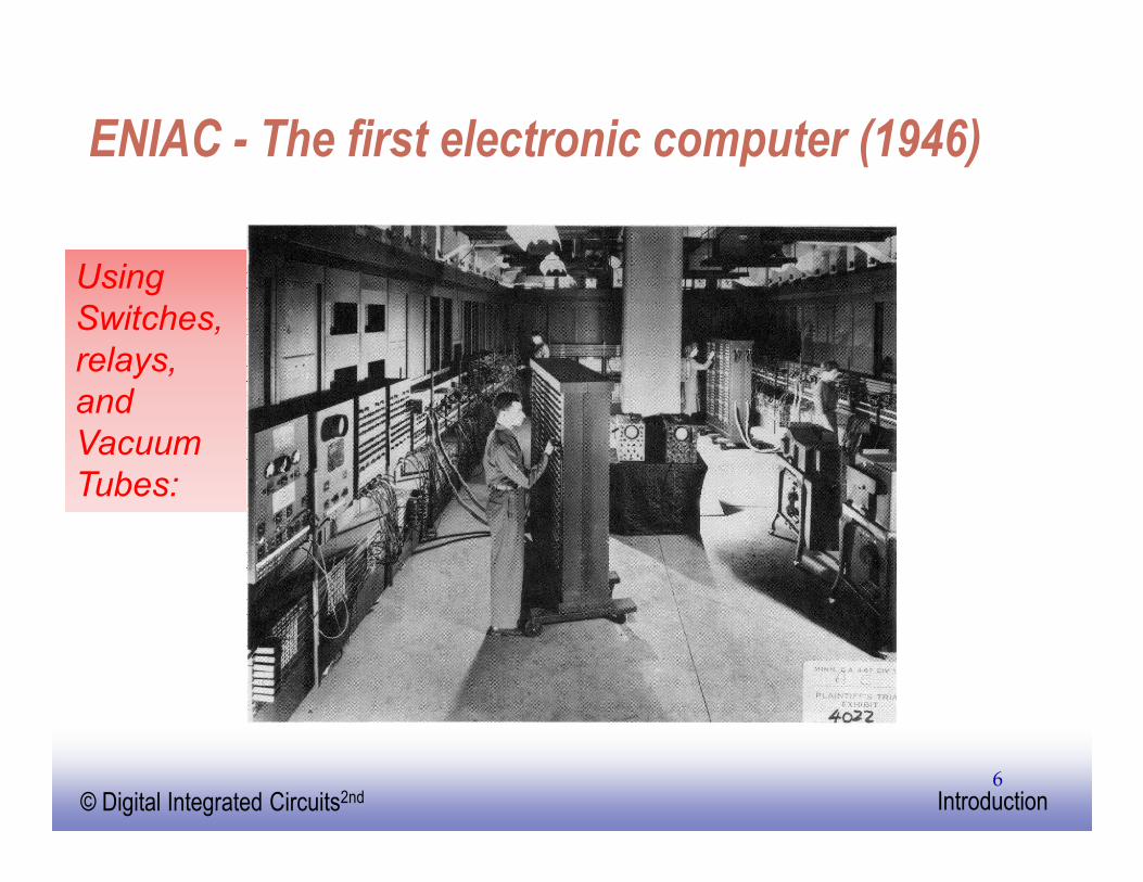
ENIAC - The first electronic computer (1946)
Using
Switches,
relays,
and
Vacuum
Tubes:
EE141© Digital Integrated Circuits2nd Introduction7
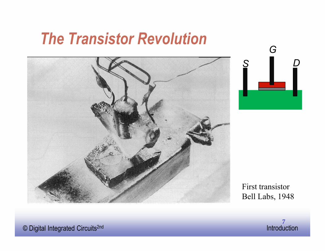
The Transistor Revolution
First transistor
Bell Labs, 1948
G
S D

EE141© Digital Integrated Circuits2nd Introduction8
The First Integrated Circuits
Bipolar logic
1960’s
ECL 3-input Gate
Motorola 1966
EE141© Digital Integrated Circuits2nd Introduction9
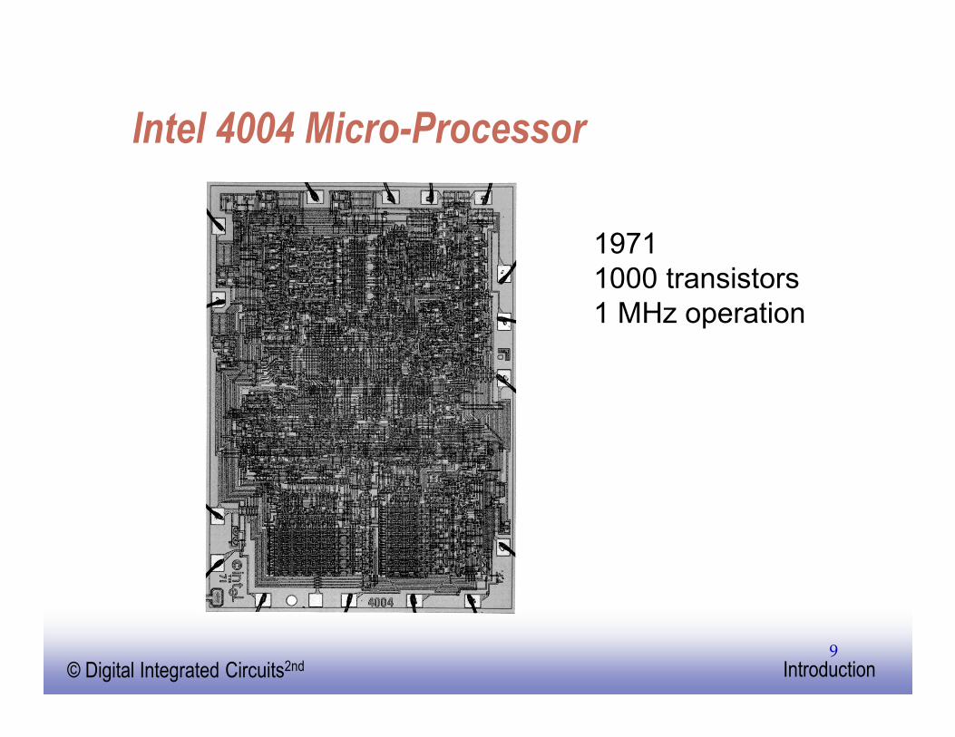
Intel 4004 Micro-Processor
19711000 transistors1 MHz operation

EE141© Digital Integrated Circuits2nd Introduction10
Intel Pentium (IV) microprocessor
EE141© Digital Integrated Circuits2nd Introduction11
Moore’s Law
�In 1965, Gordon Moore noted that the number of transistors on a chip doubled every 18 to 24 months. �He made a prediction that semiconductor technology will double its effectiveness every 18 months

EE141© Digital Integrated Circuits2nd Introduction12
Moore’s Law
16
15
14
13
12
11
10
9
8
7
6
5
4
3
2
1
0
195
9
196
0
196
1
196
2
196
3
196
4
196
5
196
6
196
7
196
8
196
9
197
0
197
1
197
2
197
3
197
4
197
5
LO
G2 O
F T
HE
NU
MB
ER
OF
CO
MP
ON
EN
TS
PE
R I
NT
EG
RA
TE
D F
UN
CT
ION
Electronics, April 19, 1965.
EE141© Digital Integrated Circuits2nd Introduction13
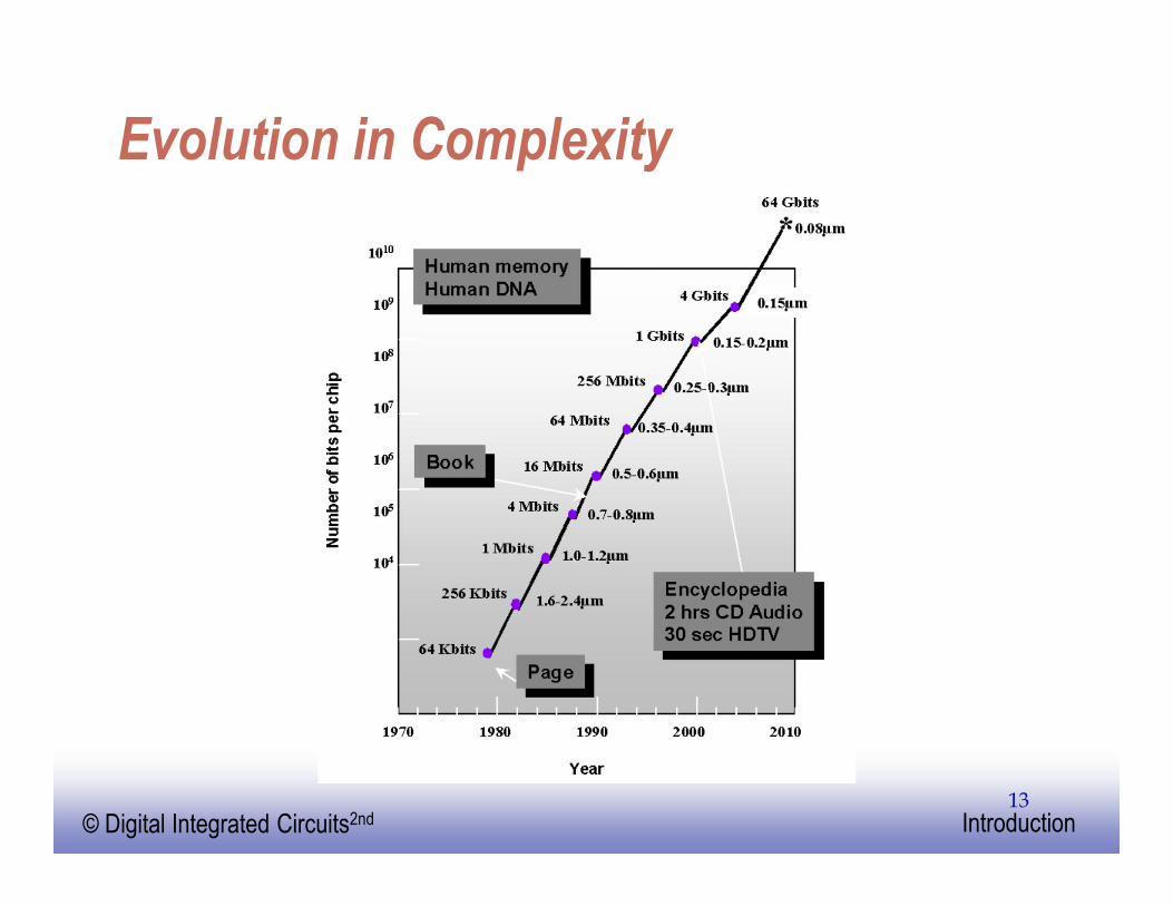
Evolution in Complexity

EE141© Digital Integrated Circuits2nd Introduction14
Transistor Counts
1,000,000
100,000
10,000
1,000
10
100
1
1975 1980 1985 1990 1995 2000 2005 2010
8086
80286i386
i486Pentium®
Pentium® Pro
K1 Billion
Transistors
Source: Intel
Projected
Pentium® II
Pentium® III
Courtesy, Intel
EE141© Digital Integrated Circuits2nd Introduction15
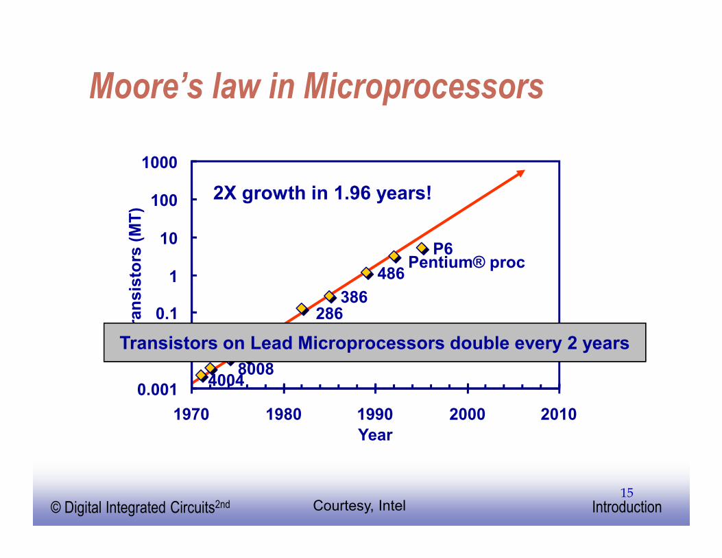
Moore’s law in Microprocessors
40048008
80808085 8086
286386
486Pentium® proc
P6
0.001
0.01
0.1
1
10
100
1000
1970 1980 1990 2000 2010
Year
Tra
nsis
tors
(M
T)
2X growth in 1.96 years!
Transistors on Lead Microprocessors double every 2 years
Courtesy, Intel
EE141© Digital Integrated Circuits2nd Introduction16
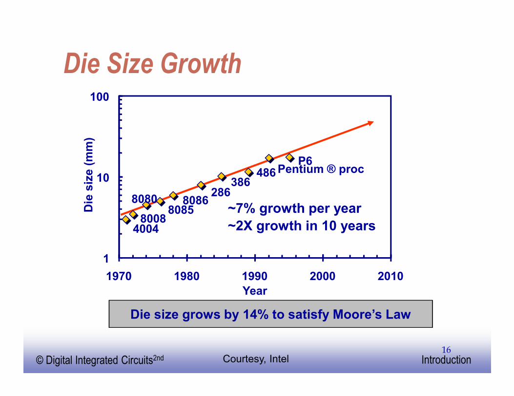
Die Size Growth
40048008
80808085
8086286
386486 Pentium ® proc
P6
1
10
100
1970 1980 1990 2000 2010
Year
Die
siz
e (
mm
)
~7% growth per year
~2X growth in 10 years
Die size grows by 14% to satisfy Moore’s Law
Courtesy, Intel

EE141© Digital Integrated Circuits2nd Introduction17
Frequency
P6
Pentium ® proc486
38628680868085
8080
80084004
0.1
1
10
100
1000
10000
1970 1980 1990 2000 2010
Year
Fre
qu
en
cy (
Mh
z)
Lead Microprocessors frequency doubles every 2 years
Doubles every2 years
Courtesy, Intel
EE141© Digital Integrated Circuits2nd Introduction18
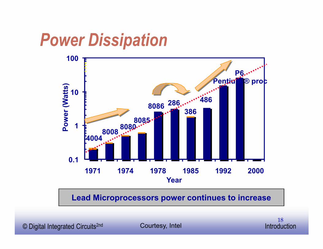
Power Dissipation
P6Pentium ® proc
486
386
2868086
80858080
80084004
0.1
1
10
100
1971 1974 1978 1985 1992 2000
Year
Po
wer
(Watt
s)
Lead Microprocessors power continues to increase
Courtesy, Intel

EE141© Digital Integrated Circuits2nd Introduction19
Power will be a major problem
5KW 18KW
1.5KW
500W
40048008
80808085
8086286
386486
Pentium® proc
0.1
1
10
100
1000
10000
100000
1971 1974 1978 1985 1992 2000 2004 2008
Year
Po
wer
(Watt
s)
Power delivery and dissipation may become prohibitive
No so-- smart designers have always found a way!!!
Power delivery and dissipation may become prohibitive
No so-- smart designers have always found a way!!!
Courtesy, Intel
EE141© Digital Integrated Circuits2nd Introduction20
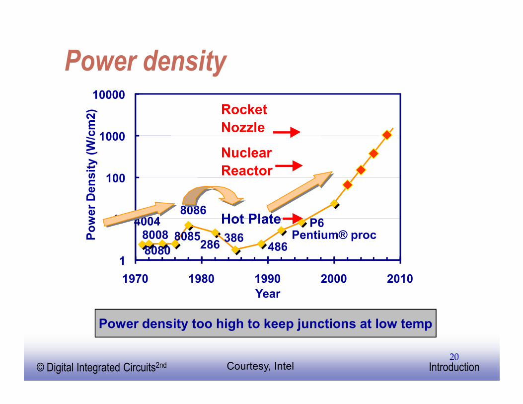
Power density
40048008
8080
8085
8086
286386
486Pentium® proc
P6
1
10
100
1000
10000
1970 1980 1990 2000 2010
Year
Po
wer
Den
sit
y (
W/c
m2)
Hot Plate
Nuclear
Reactor
Rocket
Nozzle
Power density too high to keep junctions at low temp
Courtesy, Intel
EE141© Digital Integrated Circuits2nd Introduction21
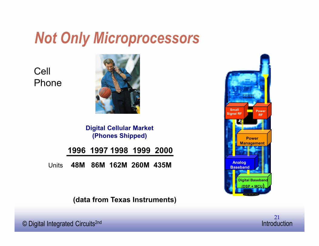
Not Only Microprocessors
Digital Cellular Market
(Phones Shipped)
1996 1997 1998 1999 2000
Units 48M 86M 162M 260M 435MAnalog
Baseband
Digital Baseband
(DSP + MCU)
Power
Management
Small
Signal RFPower
RF
(data from Texas Instruments)
CellPhone

EE141© Digital Integrated Circuits2nd Introduction22
Challenges in Digital Design
“Microscopic Problems”• Ultra-high speed design
• Interconnect
• Noise, Crosstalk
• Reliability, Manufacturability
• Power Dissipation
• Clock distribution.
Everything Looks a Little Different
“Macroscopic Issues”• Time-to-Market
• Millions of Gates
• High-Level Abstractions
• Reuse & IP: Portability
• Predictability
• etc.
Nand There’s a Lot of Them!
∝∝∝∝ 1/DSM
?
EE141© Digital Integrated Circuits2nd Introduction23
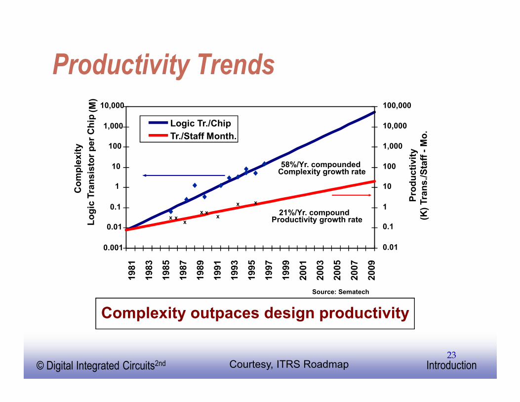
Productivity Trends
1
10
100
1,000
10,000
100,000
1,000,000
10,000,000
2003
1981
1983
1985
1987
1989
1991
1993
1995
1997
1999
2001
2005
2007
2009
10
100
1,000
10,000
100,000
1,000,000
10,000,000
100,000,000
Logic Tr./Chip
Tr./Staff Month.
xxx
xxx
x
21%/Yr. compoundProductivity growth rate
x
58%/Yr. compoundedComplexity growth rate
10,000
1,000
100
10
1
0.1
0.01
0.001
Lo
gic
Tra
nsis
tor
per
Ch
ip(M
)
0.01
0.1
1
10
100
1,000
10,000
100,000
Pro
du
cti
vit
y
(K)
Tra
ns./
Sta
ff -
Mo
.
Source: Sematech
Complexity outpaces design productivity
Co
mp
lexit
y
Courtesy, ITRS Roadmap

EE141© Digital Integrated Circuits2nd Introduction24
Why Scaling?
� Technology shrinks by ~0.7/generation
� With every generation can integrate 2x more functions per chip; chip cost does not increase significantly
� Cost of a function decreases by 2x
� But E� How to design chips with more and more functions?
� Design engineering population does not double every two yearsE
� Hence, a need for more efficient design methods� Exploit different levels of abstraction
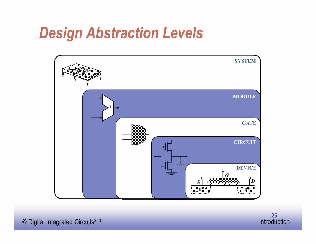
EE141© Digital Integrated Circuits2nd Introduction25
Design Abstraction Levels
n+n+
S
G
D
+
DEVICE
CIRCUIT
GATE
MODULE
SYSTEM
EE141© Digital Integrated Circuits2nd Introduction26
Design Metrics
� How to evaluate performance of a digital circuit (gate, block, E)?� Cost
� Reliability
� Scalability
� Speed (delay, operating frequency)
� Power dissipation
� Energy to perform a function

EE141© Digital Integrated Circuits2nd Introduction27
Cost of Integrated Circuits
� NRE (non-recurrent engineering) costs
� design time and effort, mask generation
� one-time cost factor
� Recurrent costs
� silicon processing, packaging, test
� proportional to volume
� proportional to chip area

EE141© Digital Integrated Circuits2nd Introduction28
NRE Cost is Increasing
EE141© Digital Integrated Circuits2nd Introduction29
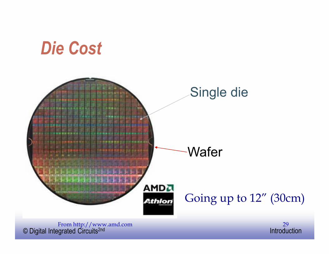
Die Cost
Single die
Wafer
From http://www.amd.com
Going up to 12” (30cm)
EE141© Digital Integrated Circuits2nd Introduction30
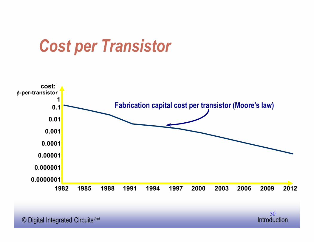
Cost per Transistor
0.0000001
0.000001
0.00001
0.0001
0.001
0.01
0.1
1
1982 1985 1988 1991 1994 1997 2000 2003 2006 2009 2012
cost: ¢-per-transistor
Fabrication capital cost per transistor (Moore’s law)

EE141© Digital Integrated Circuits2nd Introduction31
Yield
%100per wafer chips ofnumber Total
per wafer chips good of No.×=Y
yield Dieper wafer Dies
costWafer cost Die
×=
( )area die2
diameterwafer
area die
diameter/2wafer per wafer Dies
2
×
×π−
×π=

EE141© Digital Integrated Circuits2nd Introduction32
Defects
α−
α
×+=
area dieareaunit per defects1yield die
α is approximately 3
4area) (die cost die f=
EE141© Digital Integrated Circuits2nd Introduction33
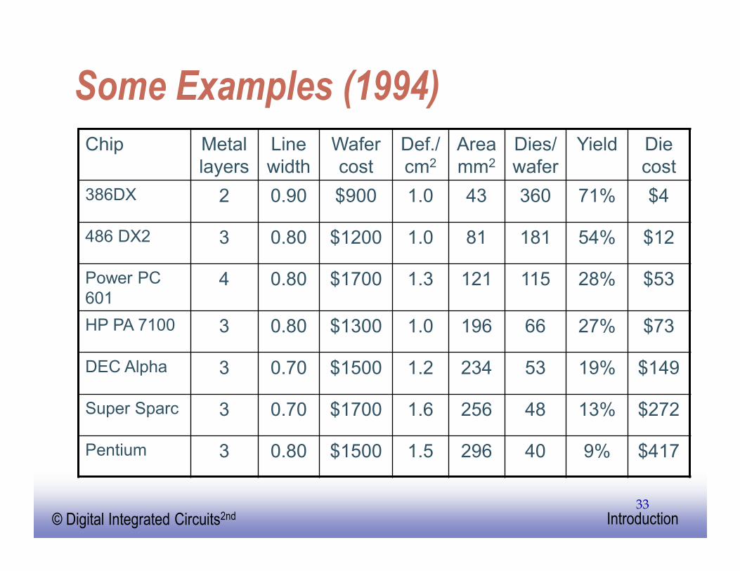
Some Examples (1994)
Chip Metal layers
Line width
Wafer cost
Def./ cm2
Area mm2
Dies/wafer
Yield Die cost
386DX 2 0.90 $900 1.0 43 360 71% $4
486 DX2 3 0.80 $1200 1.0 81 181 54% $12
Power PC 601
4 0.80 $1700 1.3 121 115 28% $53
HP PA 7100 3 0.80 $1300 1.0 196 66 27% $73
DEC Alpha 3 0.70 $1500 1.2 234 53 19% $149
Super Sparc 3 0.70 $1700 1.6 256 48 13% $272
Pentium 3 0.80 $1500 1.5 296 40 9% $417

EE141© Digital Integrated Circuits2nd Introduction34
Reliability―
Noise in Digital Integrated Circuits
i(t)
Inductive coupling Capacitive coupling Power and groundnoise
v(t) VDD

EE141© Digital Integrated Circuits2nd Introduction35
DC Operation
Voltage Transfer Characteristic
V(x)
V(y)
VOH
VOL
VM
VOH
VOL
f
V(y)=V(x)
Switching Threshold
Nominal Voltage Levels
VOH = f(VOL)VOL = f(VOH)VM = f(VM)
Will be discussed
later

EE141© Digital Integrated Circuits2nd Introduction36
Mapping between analog and digital signals
VIL
VIH
Vin
Slope = -1
Slope = -1
VOL
VOH
Vout
“ 0” VOL
VIL
VIH
VOH
Undefined
Region
“ 1”

EE141© Digital Integrated Circuits2nd Introduction37
Definition of Noise Margins
Noise margin high
Noise margin low
VIH
VIL
Undefined
Region
"1"
"0"
VOH
VOL
NMH
NML
Gate Output Gate Input
EE141© Digital Integrated Circuits2nd Introduction38
Noise Budget
� Allocates gross noise margin to expected sources of noise
� Sources: supply noise, cross talk, interference, offset
� Differentiate between fixed and proportional noise sources

EE141© Digital Integrated Circuits2nd Introduction39
Key Reliability Properties
� Absolute noise margin values are deceptive
� a floating node is more easily disturbed than a node driven by a low impedance (in terms of voltage)
� Noise immunity is the more important metric –the capability to suppress noise sources
� Key metrics: Noise transfer functions, Output
impedance of the driver and input impedance of the receiver;

EE141© Digital Integrated Circuits2nd Introduction40
Regenerative Property
v0
v1
v3
finv(v)
f (v)
v3
out
v2 in
Regenerative Non-Regenerative
v2
v1
f (v)
finv(v)
v3
out
v0 in
Will be discussed
later

EE141© Digital Integrated Circuits2nd Introduction41
Regenerative Property
A chain of inverters
v0 v1 v2 v3 v4 v5 v6
2
V (
Volt)
4
v0
v1v2
t (nsec)
02 1
1
3
5
6 8 10Simulated response
EE141© Digital Integrated Circuits2nd Introduction42
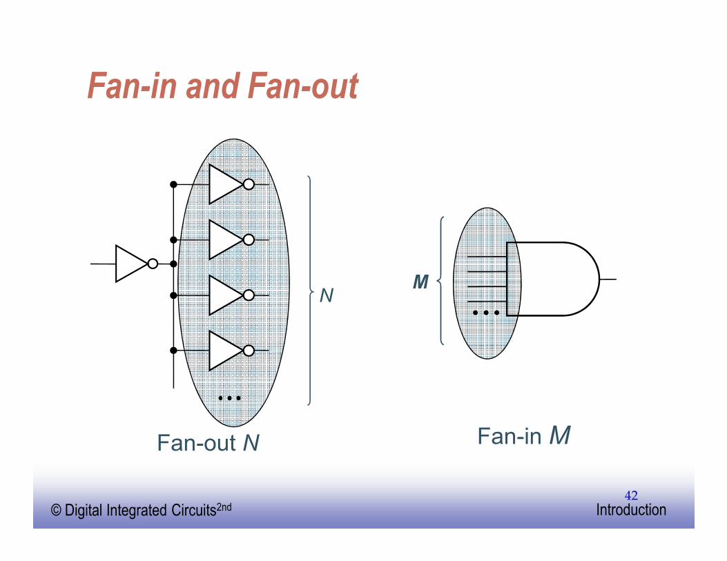
Fan-in and Fan-out
N
Fan-out N Fan-in M
M
EE141© Digital Integrated Circuits2nd Introduction43
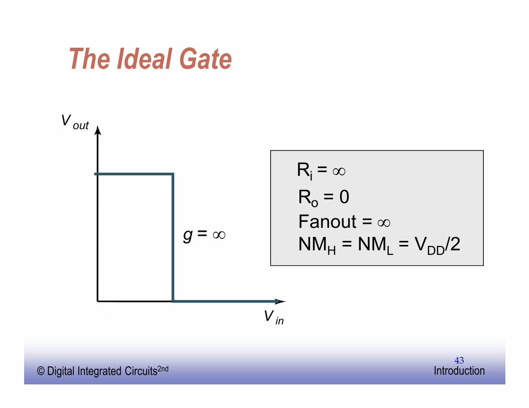
The Ideal Gate
Ri = ∞
Ro = 0
Fanout = ∞NMH = NML = VDD/2
g = ∞
V in
V out

EE141© Digital Integrated Circuits2nd Introduction44
An Old-time Inverter
NM H
V in (V)
Vout(V)
NM L
VM
0.0
1.0
2.0
3.0
4.0
5.0
1.0 2.0 3.0 4.0 5.0

EE141© Digital Integrated Circuits2nd Introduction45
Delay Definitions
Vout
tf
tpHL tpLH
tr
t
V in
t
90%
10%
50%
50%
EE141© Digital Integrated Circuits2nd Introduction46
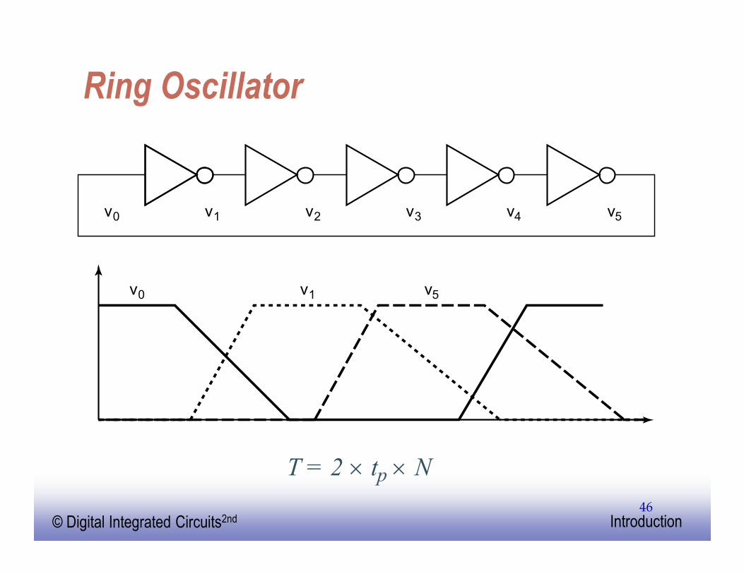
Ring Oscillator
v0 v1 v5
v1 v2v0 v3 v4 v5
T = 2 × tp × N
EE141© Digital Integrated Circuits2nd Introduction47
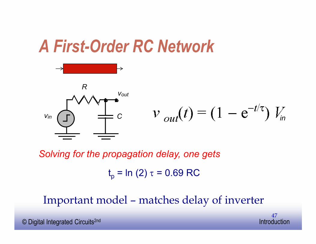
A First-Order RC Network
vout
vin C
R
tp = ln (2) τ = 0.69 RC
Important model – matches delay of inverter
in
Solving for the propagation delay, one gets

EE141© Digital Integrated Circuits2nd Introduction48
Power Dissipation
Instantaneous power:
p(t) = v(t)i(t) = Vsupplyi(t)
Peak power:
Ppeak = Vsupplyipeak
Average power:
( )∫ ∫+ +
==Tt
t
Tt
t supplysupply
ave dttiT
Vdttp
TP )(
1
t
i(t)
EE141© Digital Integrated Circuits2nd Introduction49
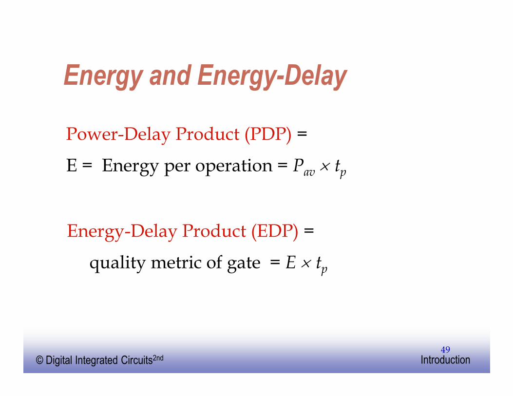
Energy and Energy-Delay
Power-Delay Product (PDP) =
E = Energy per operation = Pav × tp
Energy-Delay Product (EDP) =
quality metric of gate = E × tp

EE141© Digital Integrated Circuits2nd Introduction50
A First-Order RC Network
E0 1→ P t( )dt
0
T
∫ Vdd
isupply
t( )dt
0
T
∫ Vdd
CLdVout
0
Vdd
∫ CL
Vdd
• 2= = = =
Ecap
Pcap
t( )dt
0
T
∫ Vout
icap
t( )dt
0
T
∫ CLVout
dVout
0
Vdd
∫1
2---CL
Vdd
•2
= = = =
vout
vin CL
R

EE141© Digital Integrated Circuits2nd Introduction51
Summary
� Digital integrated circuits have come a long way and still have quite some potential left for the coming decades
� Some interesting challenges ahead� Getting a clear perspective on the challenges and
potential solutions is the purpose of this Class
� Understanding the design metrics that govern digital design is crucial� Cost, reliability, speed, power and energy
dissipation