digital image processing lectures 7 & 8 - walter scott, … quantization image transforms...
TRANSCRIPT

Image Quantization Image Transforms
Digital Image ProcessingLectures 7 & 8
M.R. Azimi, Professor
Department of Electrical and Computer EngineeringColorado State University
Spring 2015
M.R. Azimi Digital Image Processing

Image Quantization Image Transforms
Minimum Mean Squared or Lloyd-Max Quantizer
This quantizer minimizes the mean squared error (MSE) for a givennumber of quantization levels. Let the intensity of pixels in the sampledimage, x(m,n) be represented by a real, scalar, and continuous randomvariable, 0 ≤ X ≤ A, with PDF pX(x).
If the quantization error is e = x− xq, it is desired to find optimumdecision levels, tk, and reconstruction levels, rk, for an L-level quantizersuch that the MSE (or quantization distortion)
ε = E[E2] = E[(X −Xq)2] =
∫ tL+1
t1
(x− xq)2pX(x)dx
is minimized. The MSE can be rewritten as
ε =
L∑i=1
∫ ti+1
ti
(x− ri)2pX(x)dx
since xq = ri when ti ≤ x ≤ ti+1.
M.R. Azimi Digital Image Processing

Image Quantization Image Transforms
To minimize ε w.r.t. tk and rk
∂ε
∂tk= 0 ⇒ (tk − rk−1)2pX(tk)− (tk − rk)2pX(tk) = 0
∂ε
∂rk= 0 ⇒ 2
∫ tk+1
tk
(x− rk)pX(x)dx = 0, k ∈ [1, L]
where the first derivative is obtained using the fact thattk ≤ x < tk+1 ⇒ xq = rk, simplification of the above equationsgives
tk =rk + rk−1
2(1)
rk =
∫ tk+1
tkxpX(x)dx∫ tk+1
tkpX(x)dx
(2)
i.e. the optimum transition levels lie halfway between the optimumreconstruction levels, which in turn lie at the center of mass of thePDF in between the optimum transition levels.
M.R. Azimi Digital Image Processing

Image Quantization Image Transforms
These non-linear equations must be solved simultaneously giventhe bounding values t1 and tL+1. In practice, these equations canbe solved by an iterative scheme such as the Newton method.
When number of quantization levels is large, an approximatesolution can be obtained by modeling the PDF pX(x) as apiecewise constant function i.e.,
pX(x) ' pX(tj), tj∆=tj + tj+1
2, tj ≤ x ≤ tj+1
M.R. Azimi Digital Image Processing

Image Quantization Image Transforms
Using this approximation and performing the requiredminimization, the equation for optimum transition level becomes
tk+1 ≈(tL+1 − t1)
∫ akt1
[pX(x)]−1/3dx∫ tL+1
t1[pX(x)]−1/3dx
+ t1
with
ak =k(tL+1 − t1)
L+ t1, k ∈ [0, L]
Thus, this together with optimum reconstruction level in (2) i.e.rk =
tk+tk+1
2 are now de-coupled.
The quantizer MSE distortion is
ε ≈ 1
12L2∫ tL+1
t1
[pX(x)]13dx3
M.R. Azimi Digital Image Processing

Image Quantization Image Transforms
Properties of Lloyd-Max Quantizers
1 Unbiased in the mean i.e. E[X] = E[Xq].
Proof: Since Xq is a discrete r.v. with values rk, k ∈ [1, L] we have
E[Xq] =
L∑k=1
rk pXq(Xq = rk)
Using the staircase mapping of quantizer, the PMF at rk is
pXq(Xq = rk) =
∫ tk+1
tk
pX(x)dx
Thus, using Eq. (2) of Llyod-Max quantizer we get
E[Xq] =
L∑k=1
rk
∫ tk+1
tk
pX(x)dx =
L∑k=1
∫ tk+1
tk
x pX(x)dx
which can be reduced to
E[Xq] =
∫ tL+1
t1
x pX(x)dx = E[X]
M.R. Azimi Digital Image Processing
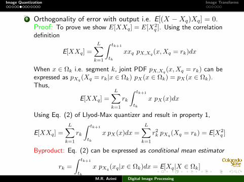
Image Quantization Image Transforms
2 Orthogonality of error with output i.e. E[(X −Xq)Xq] = 0.Proof: To prove we show E[XXq] = E[X2
q ]. Using the correlationdefinition
E[XXq] =
L∑k=1
∫ tk+1
tk
xxq pX,Xq(x,Xq = rk)dx
When x ∈ Ωk i.e. segment k, joint PDF pX,Xq (x,Xq = rk) can beexpressed as pXq
(Xq = rk|x ∈ Ωk) pX(x ∈ Ωk) = pX(x ∈ Ωk).Thus,
E[XXq] =
L∑k=1
rk
∫ tk+1
tk
x pX(x)dx
Using Eq. (2) of Llyod-Max quantizer and result in property 1,
E[XXq] =
L∑k=1
rk
∫ tk+1
tk
x pX(x)dx =
L∑k=1
r2k pXq (Xq = rk) = E[X2
q ]
Byproduct: Eq. (2) can be expressed as conditional mean estimator
rk =
∫ tk+1
tk
x pXq (xq|x ∈ Ωk)dx = E[Xq|X ∈ Ωk]
M.R. Azimi Digital Image Processing

Image Quantization Image Transforms
Remarks
1 Two commonly used PDF’s for quantization of image related dataare:
pX(x) =1√
2πσ2x
exp(− (x− µ)2
2σ2x
) Gaussian
pX(x) =α
2exp(−α|x− µ|) Laplacian
where µ is the mean, σ2x is the variance (variance of the Laplacian
PDF is σ2x = 2
α ).
2 For uniform distribution, the Lloyd-Max quantizer becomes auniform quantizer. Let
pX(x) =
1tL+1−t1 t1 ≤ x ≤ tL+1
0 otherwise
Then from (2) we get rk =(t2k+1−t
2k)
2(tk+1−tk) = tk+1+tk2 . Now combining
this result with (1) yields tk = tk+1+tk−1
2 . Thus,
tk − tk−1 = tk+1 − tk = constant∆= q.
M.R. Azimi Digital Image Processing

Image Quantization Image Transforms
Also
q =tL+1 − t1
L, tk = tk−1 + q, rk = tk + q/2
and we have rk − rk−1 = tk − tk−1 = q.i.e. all transition and reconstruction levels are equally spaced. The
quantization error e∆= x− xq is uniformly distributed over the
interval (−q/2, q/2); hence MSE is
ε =1
q
∫ q/2
−q/2α2dα =
q2
12
The variance σ2x of a uniform random variable (original image)
whose range is A is A2/12. For a uniform quantizer having B bitsL = 2B, we have q = A/2B. This gives
σ2x
ε= 22B ⇒ SNRdB = 10log1022B = 6B dB
i.e. in this special case the SNR achieved is 6dB/bit.M.R. Azimi Digital Image Processing
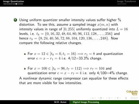
Image Quantization Image Transforms
3 Using uniform quantizer smaller intensity values suffer higher %distortion. To see this, assume a sampled image x(m,n) withintensity values in range of [0, 255] uniformly quantized into L = 16levels, i.e. tk = 0, 16, 32, 48, 64, 80, 96, 112, 128, . . . , 256 andhence rk = 8, 24, 40, 56, 72, 88, 104, 120, 136, . . . , 248. Nowcompare the following relative changes.
For x = 12 ∈ [t0 = 0, t1 = 16) =⇒ r1 = 8 and quantizationerror e = x− r1 = 4 i.e. 4/12=33.3% change.
For x = 100 ∈ [t6 = 96, t7 = 112) =⇒ r7 = 104 andquantization error e = x− r7 = 4 i.e. only 4/100=4% change.
A nonlinear dynamic range compressor can equalize for these effectsthat are more visible for low intensities.
M.R. Azimi Digital Image Processing

Image Quantization Image Transforms
Compandor Design
A compandor (compressor-expander) is a uniform quantizer proceededand succeeded by nonlinear transformations (see Fig. below-Jain’s book).
The overall system mimics a nonuniform quantizer. The decision andreconstruction levels of the compandor (nonuniform quantizer) for an even PDF,i.e. pX(x) = pX(−x), are,
tk = f−1(kq), t−k = −tk, k = 0, . . . , L/2
rk = g((k −1
2)q), r−k = −rk, k = 1, . . . , L/2
Functions f(.) (compressor) and g(.) (expander) can be found to approximateLloyd-Max quantizer without iterative process for finding tk and rk.
M.R. Azimi Digital Image Processing

Image Quantization Image Transforms
f(x) = 2a
∫ xt1
[pX(u)]1/3du∫ tL+1t1
[pX(u)]1/3du− a
g(x) = f−1(x)
where [−a, a] is the range of w = f(x) over which the uniform quantizer operates. IfpX(x) = pX(−x) i.e. even function then,
f(x) = a
∫ x0 [pX(u)]1/3du∫ tL+1
0 [pX(u)]1/3du, x ≥ 0
andf(x) = −f(−x), x < 0.
For large L, the MSE distortion of the compandor can be approximated as,
ε ≈1
12L2∫ tL+1
t1
[pX(x)]13 dx3
i.e. the same as that of the Lloyd-Max quantizer.
Note that the compandor design doesn’t generally cause the compressor outputw to be uniformly distributed.
M.R. Azimi Digital Image Processing
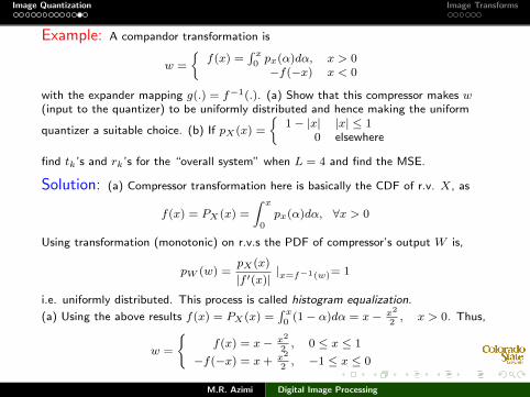
Image Quantization Image Transforms
Example: A compandor transformation is
w =
f(x) =
∫ x0 px(α)dα, x > 0−f(−x) x < 0
with the expander mapping g(.) = f−1(.). (a) Show that this compressor makes w(input to the quantizer) to be uniformly distributed and hence making the uniform
quantizer a suitable choice. (b) If pX(x) =
1− |x| |x| ≤ 1
0 elsewhere
find tk’s and rk’s for the “overall system” when L = 4 and find the MSE.
Solution: (a) Compressor transformation here is basically the CDF of r.v. X, as
f(x) = PX(x) =
∫ x
0px(α)dα, ∀x > 0
Using transformation (monotonic) on r.v.s the PDF of compressor’s output W is,
pW (w) =pX(x)
|f ′(x)||x=f−1(w)= 1
i.e. uniformly distributed. This process is called histogram equalization.
(a) Using the above results f(x) = PX(x) =∫ x0 (1− α)dα = x− x2
2, x > 0. Thus,
w =
f(x) = x− x2
2, 0 ≤ x ≤ 1
−f(−x) = x+ x2
2, −1 ≤ x ≤ 0
M.R. Azimi Digital Image Processing

Image Quantization Image Transforms
Additionally,
x = f−1(w) =
1−√
1− 2w, 0 ≤ w ≤ 1/2−1 +
√1 + 2w, −1/2 ≤ w ≤ 0
Thus, w ∼ unif [−1/2, 1/2]. Now, using a uniform quantizer with L = 4 and q = 1/4,we get quantizer’s transition and reconstruction levels,
twk = −1/2,−1/4, 0, 1/4, 1/2 ⇒ ryk = −3/8,−1/8, 1/8, 3/8
But output of the uniform quantizer y is mapped using expander transformation,
x′ = g(y) = f−1(y) =
1−√
1− 2y, 0 ≤ y ≤ 1/2−1 +
√1 + 2y, −1/2 ≤ y ≤ 0
Now, for the overall system we need to find transition levels at input x andreconstruction levels at the output of expander x′. Using the inverse functions
txk = −1,−0.293, 0, 0.293, 1 and rx′
k = −1/2,−0.134, 0.134, 1/2. Using thesevalues we can calculate MSE
ε = E[(X −X′)2] =4∑
i=1
∫ txi+1
txi
(x− rx′
i )2pX(x)dx
ε =
∫ −0.293
−1(x+0.5)2(1+x)dx+
∫ 0
−0.293(x+0.134)2(1+x)dx+
∫ 0.293
0(x−0.134)2(1−x)dx
+
∫ 1
0.293(x− 0.5)2(1− x)dx = 0.0178
M.R. Azimi Digital Image Processing

Image Quantization Image Transforms
Image Transforms
2-D unitary transforms have found numerous applications in DIP. Thefollowings are some examples.
1 Data compression using transform coding: reduce the bandwidth bydiscarding or grossly quantizing low magnitude transformcoefficients.
2 Feature extraction: extract salient features of a pattern e.g. in FThigh frequency components correspond to the edge information inthe image.
3 Dimensionality reduction to principal components: reduce thedimensionality of the image space by discarding the smallcomponents.
4 Image filtering: Wiener filter and standard 2-D filters.
M.R. Azimi Digital Image Processing

Image Quantization Image Transforms
Discrete Space Fourier Transform
The discovery of FFT for computing the DFT of sampled signals made itpossible for the Fourier analysis of signals to be performed efficientlyusing digital computers. The computational saving made possible by FFTis even more significant in the 2-D case when a large amount of data isinvolved. In what follows we start with 2-D DSFT and then show therelation between 2-D DSFT and 2-D DFT.
Spatial Sampling of Band-limited Images and DSFTWe saw that the 2-D FT of a continuous image x(u, v) is
X(ω1, ω2) =
∫ ∫ ∞−∞
x(u, v)e−jω1ue−jω2vdudv
and the inverse FT is
x(u, v) =1
4π2
∫ ∫ ∞−∞
X(ω1, ω2)ej(ω1u+ω2v)dω1dω2
M.R. Azimi Digital Image Processing
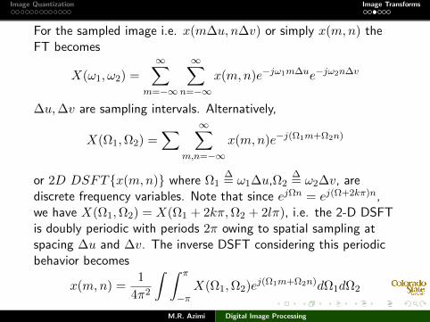
Image Quantization Image Transforms
For the sampled image i.e. x(m∆u, n∆v) or simply x(m,n) theFT becomes
X(ω1, ω2) =
∞∑m=−∞
∞∑n=−∞
x(m,n)e−jω1m∆ue−jω2n∆v
∆u,∆v are sampling intervals. Alternatively,
X(Ω1,Ω2) =∑ ∞∑
m,n=−∞x(m,n)e−j(Ω1m+Ω2n)
or 2D DSFTx(m,n) where Ω1∆= ω1∆u,Ω2
∆= ω2∆v, are
discrete frequency variables. Note that since ejΩn = ej(Ω+2kπ)n,we have X(Ω1,Ω2) = X(Ω1 + 2kπ,Ω2 + 2lπ), i.e. the 2-D DSFTis doubly periodic with periods 2π owing to spatial sampling atspacing ∆u and ∆v. The inverse DSFT considering this periodicbehavior becomes
x(m,n) =1
4π2
∫ ∫ π
−πX(Ω1,Ω2)ej(Ω1m+Ω2n)dΩ1dΩ2
M.R. Azimi Digital Image Processing

Image Quantization Image Transforms
Example 1:Determine frequency response of a 2-D system with PSF
h(m,n) =
1 |m| < M, |n| < N0 otherwise
H(Ω1,Ω2) =∑ ∞∑
m,n=−∞h(m,n)e−j(Ω1m+Ω2n)
=
M−1∑m=−M+1
N−1∑n=−N+1
e−jΩ1me−jΩ2n
Now, using∑M2
m=−M1αm = α−M1−αM2+1
1−α , |α| < 1, we get
H(Ω1,Ω2) = (e−jΩ1(−M+1) − e−jΩ1M
1− e−jΩ1)
×(e−jΩ2(−N+1) − e−jΩ2N
1− e−jΩ2)
ThenM.R. Azimi Digital Image Processing

Image Quantization Image Transforms
H(Ω1,Ω2) = (ejΩ1(M− 1
2) − e−jΩ1(M− 1
2)
ejΩ1/2 − e−jΩ1/2)
×(ejΩ2(N− 1
2) − e−jΩ2(N− 1
2)
ejΩ2/2 − e−jΩ2/2)
=sin(Ω1(M − 1/2))
sin(Ω1/2)× sin(Ω2(N − 1/2))
sin(Ω2/2)
Note that this is the aliased version of the 2-D sinc function due tothe sampling in the spatial domain (see Fig. M = 4 and N = 8).
M.R. Azimi Digital Image Processing

Image Quantization Image Transforms
Example 2:Determine the 2D DSFT of image x(m,n) = amu(m)v(n), |a| < 1where u(m) is 1-D unit step function and
v(n) =
1 0 ≤ n ≤ N − 10 elsewhere
X(Ω1,Ω2) =∑ ∞∑
m,n=−∞x(m,n)e−j(Ω1m+Ω2n)
=
∞∑m=−∞
amu(m)e−jΩ1m∞∑
n=−∞e−jΩ2nv(n)
=
∞∑m=0
ame−jΩ1mN−1∑n=0
e−jΩ2n
= (1
1− ae−jΩ1)× e−jΩ2( N−1
2 ) sin(NΩ2/2)
sin(Ω2/2)
M.R. Azimi Digital Image Processing