differential equations for chemical kinetics · differential equations for chemical kinetics...

Differential equations forchemical kinetics

Atmospheric Modelling course

Sampo [email protected]

15.11.2010

Sampo Smolander Chemical kinetics 15.11.2010 1 / 24

Chemical equation

reactants → products : rate coefficient

SO3 +H2O → H2SO4 : 5.0−15

∂[H2SO4]

∂t= k1[SO3][H2O]

∂[SO3]

∂t= −k1[SO3][H2O]

∂[H2O]

∂t= −k1[SO3][H2O]

k1 = 5.0−15 mol/s


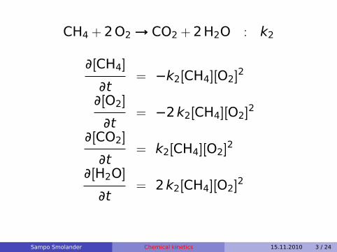
CH4 + 2O2→ CO2 + 2H2O : k2

∂[CH4]

∂t= −k2[CH4][O2]

2

∂[O2]

∂t= −2k2[CH4][O2]

2

∂[CO2]

∂t= k2[CH4][O2]

2

∂[H2O]

∂t= 2k2[CH4][O2]

2


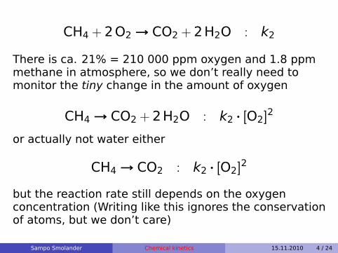
CH4 + 2O2→ CO2 + 2H2O : k2

There is ca. 21% = 210 000 ppm oxygen and 1.8 ppmmethane in atmosphere, so we don’t really need tomonitor the tiny change in the amount of oxygen

CH4→ CO2 + 2H2O : k2 · [O2]2

or actually not water either

CH4→ CO2 : k2 · [O2]2

but the reaction rate still depends on the oxygenconcentration (Writing like this ignores the conservationof atoms, but we don’t care)


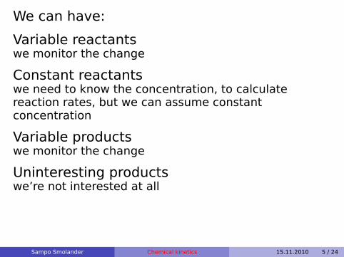
We can have:

Variable reactantswe monitor the change

Constant reactantswe need to know the concentration, to calculatereaction rates, but we can assume constantconcentration

Variable productswe monitor the change

Uninteresting productswe’re not interested at all


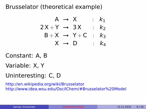
Brusselator (theoretical example)

A → X : k1

2X+ Y → 3X : k2

B+X → Y+C : k3

X → D : k4

Constant: A, B

Variable: X, Y

Uninteresting: C, Dhttp://en.wikipedia.org/wiki/Brusselatorhttp://www.idea.wsu.edu/OscilChem/#Brusselator%20Model


http://en.wikipedia.org/wiki/Brusselator

http://www.idea.wsu.edu/OscilChem/#Brusselator%20Model

A→ X ∂[X]∂t

= −k1[A]

2X+ Y→ 3X∂[X]∂t

= k2[X]2[Y]∂[Y]∂t

= −k2[X]2[Y]

B+X→ Y+C∂[X]∂t

= −k3[X][B]∂[Y]∂t

= k3[X][B]

X→ D ∂[X]∂t

= −k4[X]

We don’t need to write equations for A, B because theystay constant

And C, D we are not interested in


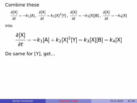
Combine these

∂[X]

∂t= −k1[A] ,

∂[X]

∂t= k2[X]2[Y] ,

∂[X]

∂t= −k3[X][B] ,

∂[X]

∂t= −k4[X]

into

∂[X]

∂t= −k1[A] + k2[X]2[Y]− k3[X][B]− k4[X]

Do same for [Y], get...


∂[X]

∂t= −k1[A] + k2[X]2[Y]− k3[X][B]− k4[X]

∂[Y]

∂t= −k2[X]2[Y] + k3[X][B]

Or with more chemicals and reactions, you’lljust get a larger system of coupled differentialequations. But the principle is easy?

Next: numerics


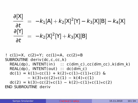
∂[X]

∂t= −k1[A] + k2[X]2[Y]− k3[X][B]− k4[X]

∂[Y]

∂t= −k2[X]2[Y] + k3[X][B]

! c(1)=X, c(2)=Y; cc(1)=A, cc(2)=BSUBROUTINE deriv (dc , c , cc , k)

REAL(dp) , INTENT( in ) : : c (dim_c) , cc (dim_cc) ,k(dim_k)REAL(dp) , INTENT(out ) : : dc(dim_c)dc(1) = k(1)*cc(1) + k(2)*c(1)*c(1)*c(2) &

− k(3)*cc(2)*c(1) − k(4)*c(1)dc(2) = k(3)*cc(2)*c(1) − k(2)*c(1)*c(1)*c(2)

END SUBROUTINE deriv


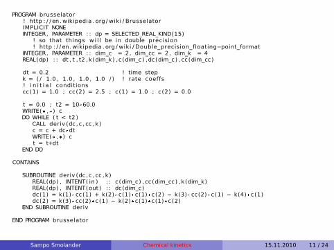
PROGRAM brusselator! http : / / en. wikipedia . org / wiki / BrusselatorIMPLICIT NONEINTEGER, PARAMETER : : dp = SELECTED_REAL_KIND(15)

! so that things w i l l be in double precision! http : / / en. wikipedia . org / wiki / Double_precision_floating−point_format

INTEGER, PARAMETER : : dim_c = 2, dim_cc = 2, dim_k = 4REAL(dp) : : dt , t , t2 , k(dim_k) , c (dim_c) ,dc(dim_c) , cc (dim_cc)

dt = 0.2 ! time stepk = ( / 1.0 , 1.0 , 1.0 , 1.0 / ) ! rate coeffs! i n i t i a l conditionscc(1) = 1.0 ; cc(2) = 2.5 ; c(1) = 1.0 ; c(2) = 0.0

t = 0.0 ; t2 = 10*60.0WRITE(* ,*) cDO WHILE ( t < t2 )

CALL deriv (dc , c , cc , k)c = c + dc*dtWRITE(* ,*) ct = t+dt

END DO

CONTAINS

SUBROUTINE deriv (dc , c , cc , k)REAL(dp) , INTENT( in ) : : c (dim_c) , cc (dim_cc) ,k(dim_k)REAL(dp) , INTENT(out ) : : dc(dim_c)dc(1) = k(1)*cc(1) + k(2)*c(1)*c(1)*c(2) − k(3)*cc(2)*c(1) − k(4)*c(1)dc(2) = k(3)*cc(2)*c(1) − k(2)*c(1)*c(1)*c(2)

END SUBROUTINE deriv

END PROGRAM brusselator


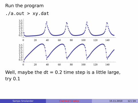
Run the program

./a.out > xy.dat

0 20 40 60 80 100 120 140

0.51.01.52.02.53.03.5

0 20 40 60 80 100 120 140

0.51.01.52.02.53.03.5

Well, maybe the dt = 0.2 time step is a little large,try 0.1


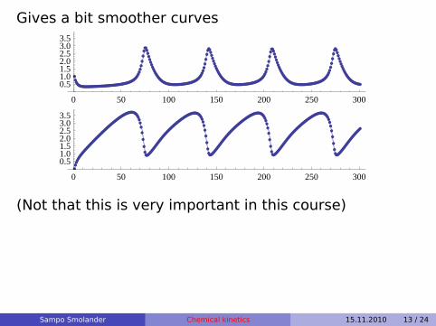
Gives a bit smoother curves

0 50 100 150 200 250 300

0.51.01.52.02.53.03.5

0 50 100 150 200 250 300

0.51.01.52.02.53.03.5

(Not that this is very important in this course)


A system of differential equations can be expressed asone vector-valued equation

∂C

∂t= f(C, t)

C = (c1,c2, . . .) are the chemical concentrationsand f gives the derivatives

�

∂c1∂t ,

∂c2∂t , . . .�

f may or may not depentd on t


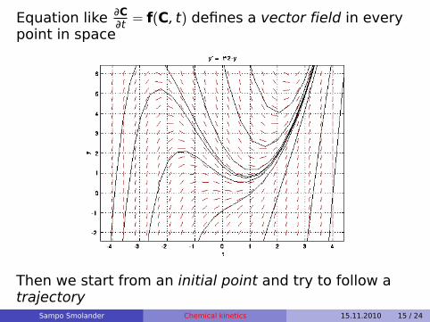
Equation like ∂C∂t = f(C, t) defines a vector field in every

point in space

Then we start from an initial point and try to follow atrajectory


In the previous code, we are at some stateC(t), then we evaluate the derivative at thisstate, and take a step to that direction

This is called the Euler methodhttp://en.wikipedia.org/wiki/Euler_method

It is the simplest, but also most imprecisemethod for solving differential equationsnumerically

It is good enough for this course, but I justwant to mention one another method


http://en.wikipedia.org/wiki/Euler_method

Maybe the derivative changes during thestep?

With stepsize dt = h we step from C(t) toC(t + h) just following the direction ∂C(t)

∂tbut at

C(t + h) we should already be going todirection ∂C(t+h)

∂t

Next: Runge-Kutta method


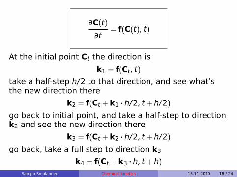
∂C(t)

∂t= f(C(t), t)

At the initial point Ct the direction is

k1 = f(Ct, t)

take a half-step h/2 to that direction, and see what’sthe new direction there

k2 = f(Ct +k1 · h/2, t + h/2)

go back to initial point, and take a half-step to directionk2 and see the new direction there

k3 = f(Ct +k2 · h/2, t + h/2)

go back, take a full step to direction k3

k4 = f(Ct +k3 · h, t + h)Sampo Smolander Chemical kinetics 15.11.2010 18 / 24

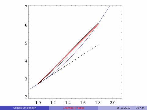
1.0 1.2 1.4 1.6 1.8 2.02

3

4

5

6

7


Now, Ct +k3 · h would already be a good step, but we’renot done yet. We have 4 different candidates for the“right” direction to go

k1,k2,k3,k4

Take a weighted average

k = 1/6 (k1 + 2k2 + 2k3 +k4)

and go thereCt+1h = Ct +k · h

This is the Runge-Kutta method

http://en.wikipedia.org/wiki/Runge-Kutta_methods


http://en.wikipedia.org/wiki/Runge-Kutta_methods

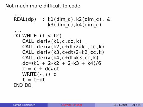
Not much more difficult to code

. . .REAL(dp) : : k1(dim_c) ,k2(dim_c) , &

k3(dim_c) ,k4(dim_c). . .

DO WHILE ( t < t2 )CALL deriv (k1 , c , cc , k)CALL deriv (k2 , c+dt /2*k1, cc , k)CALL deriv (k3 , c+dt /2*k2, cc , k)CALL deriv (k4 , c+dt*k3, cc , k)dc=(k1 + 2*k2 + 2*k3 + k4)/6c = c + dc*dtWRITE(* ,* ) ct = t+dt

END DO


0 5 10 15 20 25 30

0.51.01.52.02.53.03.5

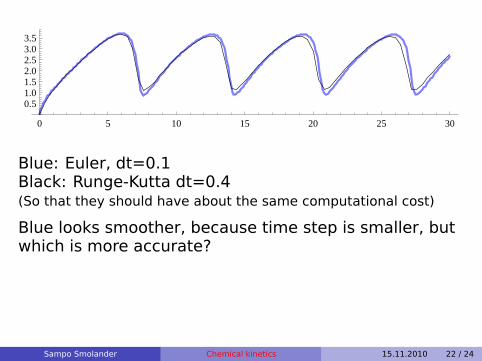
Blue: Euler, dt=0.1Black: Runge-Kutta dt=0.4(So that they should have about the same computational cost)

Blue looks smoother, because time step is smaller, butwhich is more accurate?


0 5 10 15 20 25 30

0.51.01.52.02.53.03.5

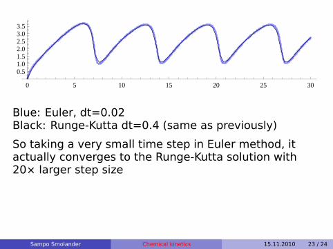
Blue: Euler, dt=0.02Black: Runge-Kutta dt=0.4 (same as previously)

So taking a very small time step in Euler method, itactually converges to the Runge-Kutta solution with20× larger step size


Now you should be able to:

– read chemical equations

– write the corresponding system ofdifferential equations

– code numerical solution to the DE’sRunge-Kutta is by no means very advanced algorithmeither. In real work, we use algorithms with adaptivestep size, and we use existing libraries and don’t codethe solvers ourselves

More information: “numerical analysis” / “numericalmethods” / “differential equations” textbooks.Google: ’ODE solvers’, ’Stiff equations’


differential equations for chemical kinetics · differential equations for chemical kinetics...

Documents