development of real time data visualization and analysis … · acquisition, analysis, simulation,...
TRANSCRIPT

Development of Real Time Data Visualization and Analysis Software for the
National Synchrotron Light Source II (NSLS-II) X-ray Powder Diffraction (XPD)
Beam Line
By
Caleb Duff
A senior thesis submitted to the faculty of Brigham Young University- Idaho in partial
fulfillment of the requirements for the degree of
Bachelor of Science
Department of Physics and Astronomy
Brigham Young University – Idaho
December 2016

Copyright © 2016 Caleb Duff
All Rights Reserved

Brigham Young University-Idaho
DEPARTMENT APPROVAL
Of a Senior Thesis submitted by
Caleb Duff
This thesis has been reviewed by the research advisor, research committee, and the department
chair and has been found to be satisfactory.
___________________ ____________________________________________________
Date Stephen McNeil, Department Chair and Advisor
___________________ ____________________________________________________
Date Lance Nelson, Committee Member
___________________ ____________________________________________________
Date David Oliphant, Committee Member
___________________ ____________________________________________________
Date Evan Hansen, Committee Member


Abstract
X-ray powder diffraction is an x-ray beam technique that allows scientists to gain
information about the underlying crystal structure of materials. In one year of operation, the
NSLS-II XPD beam line has already enabled a great diversity of experiments in areas such as
next generation batteries, catalysis, ultra-high temperature ceramics, structural nuclear materials,
pharmaceutical drugs and high-temperature superconductor flux growth. A long term software
development plan is underway to make software that supplies the beam line’s needs for data
acquisition, analysis, simulation, and visualization.
My project focused on creating software that enables beam line users to interact with
their data acquired at the beam line in real time. The data can be presented in many ways,
allowing the users to be confident in measurement that they are taking while working here at
Brookhaven National Laboratory.

Acknowledgements
I want to say thank you to all XPD beam line staff who helped me to make software for
them. Chia-Hao Liu deserves special thanks for working with me on this project. Tom Caswell
and Chris Wright as well for their computer savvy and advice. I want to especially thank my
mentor for his patience and help in making a platform that will be useful to the beam line.
This project was supported in part by the U.S. Department of Energy, Office of Science,
Office of Workforce Development for Teachers and Scientists (WDTS) under the Science
Undergraduate Laboratory Internships Program (SULI).

Table of Contents
1. Introduction
1.1. Crystal Structures
1.2. Bragg’s Law
1.3. X-ray Powder Diffraction
1.4. The Author’s Role
2. Methods
2.1. Software Workflow
2.2. Data Acquisition
2.2.1. From File
2.2.2. Detector Live Streaming
2.3. Interactive Visualization
2.3.1. Direct Diffraction Data
2.3.2. Displaying One Dimensional Reduced Data
2.3.3. Two Dimensional Waterfall Plot of Reduced Data
2.3.4. Three Dimensional Modeling of Reduced Data
2.3.5. Peak Searching
2.3.6. Common Statistical Parameters
2.4. Analysis
2.4.1. One Dimensional Integrated Data Reduction
2.4.2. Peak Searching
2.4.3. Statistical Parameter Calculation
3. Results

3.1. Brief Overview
3.2. Current Software Capabilities
3.2.1. Data Acquisition
3.2.2. Direct Diffraction Data Implementation
3.2.3. One Dimensional Reduced Data Display Results
3.2.4. Two Dimensional Waterfall Plot of One Dimensional Reduced Data Results
3.2.5. Three Dimensional Modeling of Reduced Data Results
3.2.6. Peak Searching Results
3.2.7. Common Statistical Parameters
3.2.8. One Dimensional Integrated Data Results
3.3. Software Specifications
4. Conclusion
5. References

List of Figures
Figure 1 Example of crystal lattice structures and arrangement of atoms. (Materials, 2016) .. - 11 -
Figure 2 Visualization of the way that x-rays scatter off of some sample being analyzed. (Why,
2016) ................................................................................................................................. - 12 -
Figure 3 Example of diffraction data obtained from the machinery at the beam line. This is a
Cerium Oxide sample. The units in the graph are pixel numbers and are unitless. Please note
as well, that all data shown to demonstrate the software is using this Cerium Oxide sample.
Cerium Oxide is a Fluorite Cubic in crystal structure. ..................................................... - 13 -
Figure 4 1D integrated pattern of the previous 2D diffraction data. Radius refers to distance from
center of the detector image. This is obtained through Bragg's law and various geometrical
properties of the machinery setup. The actual units will be discussed further in the results
section. .............................................................................................................................. - 14 -
Figure 5 This figure is an overall description of what the software design goals were, and how
they were to interact with each other to achieve software design goals. ................................ 2
Figure 6 This picture is the current look of the software. This image was taken on my computer. 9
Figure 7 Toolbox for changing two dimensional plot window. .................................................... 11
Figure 8 Peak searching plot in current version. Units were asked to be omitted by the scientists,
as they correspond exactly to those on the 1D reduced representation of the data, and were
seen as unnecessary for repetition. ........................................................................................ 12
Figure 9 Dialog window for creating statistical parameters plot. ................................................. 13

Figure 10 This dialog window controls the parameters used by the PyFAI library during the
integration process. ............................................................................................................... 14

1 Introduction and Background
At the X-ray Powder Diffraction (XPD) beam line a variety of different environments can be
simulated. The staff can increase the pressure and/or temperature a beam line user’s sample is
under. Changes to the sample’s gas environment are also available. Data can be recorded over
time in all of these situations to see what happens to the crystal structure of the materials and
details how and when a phase change occurs, or checking the structural changes during chemical
reactions, are important to know. This information can lead us to better understand the chemical
reactions happening on an atomic level, teaches us under what conditions a material has a stable
structure, and leads to improvements in battery materials (L. Wangoh, 2016), nuclear reactor
structural materials (D. Sprouster, 2015), and a growth of knowledge in many other fields that
would otherwise not be possible. (K Wang, 2015), (B Fradsen, 2016), (J Arinez-Soriano, 2016)
1.1 Crystal Structures
There are many materials around us that are formed by crystal structures. A crystal is simply any
atomic pattern that repeats itself in building blocks to create a structure. Some great examples of
this are salt, sugar, metals, etc. Understanding how the structure of a material affects its
properties is one of the driving reasons for pursuing research with X-ray Powder Diffraction
(XPD).
1.2 Bragg’s Law
Light when it enters some crystal structure is prone to diffract, or scatter, based off of the spacing
of the atoms. This relationship can be expressed with the following equation 2𝑑 sin 𝜃 = 𝑛𝜆.
We define the angle theta, 𝜃, to be the angle that the x-rays diffract at that leads to constructive

interference. Lambda, 𝜆, is the wavelength of the x-rays involved in the process. The letter d
simply refers to the spacing of the atoms in the crystal. (Girolami, 2016) This relationship simply
shows where the x-rays will constructively interfere to produce the patterns that will be discussed
later. The variety of peaks that appear come from the fact that not all atoms are spaced the same
amount in crystal lattices. Different crystal structures have different shapes, and this causes the
patterns to appear different.
Figure 1 Example of crystal lattice structures and arrangement of atoms. (Materials, 2016)
1.3 X-ray Powder Diffraction.
By sending in a beam of x-rays into some sample, light will come off in cone shapes that can be
captured by a detector placed a specific distance away. The following figure gives a visualization
of this idea. The reason powders are used is to create these circular patterns, if a single crystal
were to be used, all that would be seen are bands of light going up the wall.

Figure 2 Visualization of the way that x-rays scatter off of some sample being analyzed. (Why, 2016)

The detector can then capture these light patterns in an image like the following.
Figure 3 Example of diffraction data obtained from the machinery at the beam line. This is a Cerium Oxide sample. The units in the graph are pixel numbers and are unitless. Please note as well, that all data shown to demonstrate the software is using this Cerium Oxide sample. Cerium Oxide is a Fluorite Cubic in crystal structure.
It is important to note in the previous figure that this is a false color image. X-rays are not visible
to the human eye, so this image has been given color. Darker regions show areas where light is
not strongly diffracted to and brighter areas show regions where light is strongly diffracted to.
The pattern of rings can tell us what is the crystal structure of the material.
X-ray powder diffraction uses this idea to find out the structural features at the atomic
scale of some sample material. From this information we can learn about any symmetries found
in the crystal, the coordinates of each atom within its crystal lattice, and how well organized the

atoms are in their structure. The location of the atoms relative to each other can be found, the
charge distribution, and all symmetries in the crystal. Comparing the measured diffraction image
with data collected from structure databases makes it possible to identify the structural phase of
the material.
Normally the rings are integrated azimuthally to create some 1D image that can display
this information more clearly. These 1D integration patterns can look like the following.
Figure 4 1D integrated pattern of the previous 2D diffraction data. Radius refers to distance from center of the detector image. This is obtained through Bragg's law and various geometrical properties of the machinery setup. The actual units will be discussed further in the results section.
This is easier to obtain than information from the rings, in that we can model the measured 1D
profile of the rings. Through some mathematics based on this profile information we can find the
crystal symmetry of the system, the lattice dimensions, and the position of the atoms.

The great thing about XPD is that the environment the sample is placed in does not need
to be static to gain information about the sample’s crystal structure. We can obtain this
information in a variety of situations as mentioned previously. This is where the beam line comes
in, along with the need for this software.
1.4 The Author’s Role
The software that was worked on this summer by the author allows all of this information to be
gathered in one place and viewed by scientists while the measurements are occurring. The
software allows them to see all of these diffracted image patterns together and manipulate these
images to assess the quality and readability of the measurement.


2 Methods Section
Figure 5 This figure is an overall description of what the software design goals were, and how they were to interact with each other to achieve software design goals.
A long term software development plan is underway to provide software that can access
the detector to save diffraction pattern images, process these images into integrable data, display
the data, and provide live analysis of the data. The hope is that this software will become
sophisticated enough to do complex analysis of data during live experiments at the beam line.
Much of the software is already developed that captures the images, but visualization has
been tricky to do. This is because the detectors used to capture the X-ray powder diffraction
patterns are of high resolution. This means that they contain a lot of data that is difficult to read
in quickly by a computer. The software developed needed to synchronize well with what on-site

groups had already accomplished and also work quicker than what had been previously
implemented. Previous software was only able to measure images at a rate of about one image
per minute, but the detectors have the potential to take images at a rate of about ten images per
second. This leaves a backlog that can accrue very quickly and slow down experiments being
performed by scientists at the beam line.
Python is the coding language that is officially used at NSLS-II, so this software was
tailored to fit laboratory standards and was created in Python. It relies heavily on the pyQT,
Matplotlib, and PyFAI libraries found in the python language. pyQT is a python library that
focuses on user interfacing to allow live software to be interacted with in a live setting. (Page,
2016) Matplotlib is software devoted to data display in a clean, sensible format. (Introduction,
2016) PyFAI is software that focuses on azimuthal integration of large images that takes many
factors into account, such as image rotation and beam deviation, to give the quickest and most
accurate azimuthal integration of the diffraction data. (PyFAI, 2016)
Through various meetings with the beam line staff, a work plan to develop this software
was created. The work plan contained data capture, interactive visualization, and analysis. Data
capture is the process where the computer obtains the data. Interactive visualization refers to the
ability of the software to handle image rendering and also allow the user to manipulate the data
to assess the quality. Analysis is the software’s ability to print out useful information about the
data so that the user can obtain useful information about their data.
2.2 Data Acquisition
As mentioned previously the diffraction data is saved in the form of .tif files that are 16
megabytes in size. The rate at which these files are produced is extremely high. It is important
that the software have the ability to read a large number of files quickly, without taking up too
much space in the RAM of the computer to allow for easy displaying and data analysis. There
are two methods that were asked for by beam line staff to read in data from file and live
streaming from the detectors.
2.2.1 From File
To read from file means simply that the diffraction pattern is taken by the machine,
operated on and put into a file format, and then saved to the computer to be accessed later. Beam
line staff were hoping that there would be a quick and easy way to take the diffraction patterns
already stored on beam line computers and then read them into the software for later
visualization and analysis. The staff decided that it would be best if the software had a dialog
option or button press, that would allow software users to pull up a window that allows them to
select files directly. The software would then take these files and then read them in to be used
later. The files follow the basic format of a two dimensional array and contain the intensity of
light found at the point on the detector. The file simply records this in an easy to read format.
(Tifffile, 2016)
2.2.2 Detector Live Streaming
Live streaming data is the process by which instead of saving data into some file format,
the detector just sends data directly from its components to the computer. It is possible to save
the data as a background process while doing this, but the major benefit of using this method is
that there is significantly less computer power and memory being expended to read or write files.
This would speed up software performance greatly and take up fewer computer resources since
we are simply sending the two dimensional intensity array into the computer for analysis and

visualization. This is quicker than having the computer use various algorithms to prep the data
for storage and then store the data, followed by reopening the data for viewing.
2.3 Interactive Visualization
It is great that we have the ability to take data and save it, or send it into the computer.
But what do we do with it after that? This is where interactive visualization becomes important.
After obtaining the data the software needs to be able to take that data and display it
meaningfully to users. The following sections will discuss what beam line staff requested.
2.3.1 Direct Diffraction Data
One of the most important things to know about the diffraction patterns is what they look
like. As shown in the introduction, when a sample is bombarded with x-rays, the x-rays are
reflected off and create ring like patterns. Due to the high levels of radiation provided by NSLS-
II the area where the sample is kept must be shut off from the surrounding environment.
Scientists need to make sure that while conducting their experiments, that quality data is being
collected. Scientists must also be assured that the equipment is working properly. By seeing the
original diffraction patterns we can know if the sample is improperly mounted, if the x-rays from
the synchrotron source are coming in at regular amounts, and that the detector is observing
patterns with the shutter open.
Also with this comes the need to be able to change the way the direct diffraction data is
viewed. This means changing the intensity scaling on the image and color map. X-rays are a kind
of light that do not fall in the visible part of the light spectrum. In order observe the diffraction
patterns directly, false color images are used to see where the highest number of x-rays were
found. Higher intensities are associated with certain colors on the color map and lower intensities

are associated with other colors. This allows the ring like patterns to be seen. It is important to be
able to change the intensity scaling to allow scientists to see rings of various intensities. They
might have their own reasons for this and so the option is left for them. The users should also be
able to skim through images quickly, zoom in on certain regions of the image, and be able to
save the current view and format of the image they have created.
2.3.2 Displaying One Dimensional Reduced Data
A plot must also be available for the one dimensional reduced data. It should contain
relevant information about which diffraction pattern is being observed. The plot must also clearly
display the relative intensities between atomic spacings and fit a line to the data. The process for
getting this data will be discussed in analysis under one dimensional integrated data reduction.
2.3.3 Two Dimensional Waterfall Plot of Reduced Data
It is helpful to see how a sample is changing its atomic spacing over time. To allow
scientists to observe this, it was requested that the software give the option to stack the one
dimensional reduced patterns on top of each other for quick comparison. A toolbox should also
be added to allow the option of normalizing the reduced data patterns and change the spacing on
the waterfall between the patterns in the horizontal and vertical direction.
2.3.4 Three Dimensional Modeling of Reduced Data
This style of plot is similar to waterfall plot of reduced data. The major difference is that
the peaks and flow of the atomic spacing is more pronounced on a three dimensional graph,
whereas on the two dimensional graph it easier to see the patterns in overall shape of the graphs.

2.3.5 Peak Searching
The software should also include the ability to track peaks on the one dimensional data
reduction over time. This chart should only show the file location and the location of the peaks
on that file. This chart should also have the option of clicking on a certain peak. This should lead
to the corresponding diffraction pattern and reduced data plot being pulled up to be viewed by
the user.
2.3.6 Common Statistical Parameters
The software user should be able to zoom in on a region of the diffraction data and then
find some statistical parameter associated with that region. These parameters include, but are not
limited to: standard deviation of x-ray intensity in that region, mean intensity of x-ray intensity in
region, the minimum intensity of the region, and the maximum intensity found in that region.
The plot should have properties similar to the peak searching plot, in that clicking on a specific
data point should pull up the corresponding diffraction pattern and one dimensional reduced data
of that pattern.
2.4 Analysis
2.4.1 One Dimensional Integrated Data Reduction
The next step common step to use in analyzing diffraction data is to process the data
using azimuthal integration. This entails summing the ring’s intensities to find the intensity of
that ring at a certain distance from the center of the detector. Through Bragg’s law and various
geometry principles, the atomic spacing can then be found. The intensity relative to that ring can
then inform the scientists as to how often you find atoms of a certain spacing relative to other

atoms. This then gives information that scientists seek to know about the materials they bring in
as discussed in the introduction.
A box should appear before the integration process begins to allow scientists to input
certain parameters for their analysis. These parameters should include: x-ray wavelength used in
experiment, distance from detector to sample, rotation of detector along XY and YZ plane, and
the center of the detector relative to the images recorded.
2.4.2 Peak Searching
The easiest thing to do for peak searching is to find the relative maxima of the peaks in
some region. An algorithm was created to set certain parameters for what counted as a peak and
what did not. The main requirement for a peak to be considered, is that it must be a higher value
than any other part of the plot within so many spaces. If this requirement is meant, it would then
be recorded as a peak.
2.4.3 Statistical Parameter Calculation
Another algorithm was developed to compute basic values as mentioned previously. The
software uses the basic equation for calculating mean, maximum, minimum, standard deviation,
and total intensity in the region selected by the user. The region is determined using the zoom
option found with the direct diffraction data plot.

3 Results
This section will discuss current software capabilities and how the software was tested to
ensure quality standards were met. This section will mostly follow the format of the methods
section and be followed by testing results. Please note as well that the title of the software was
decided to be XPD View and from hence forth will be referred to as such.
3.2 Current Software Capabilities
Figure 6 This picture is the current look of the software. This image was taken on my computer.
The image above shows XPD View in its current version. As can be seen many of the
functionalities requested by beam line staff have been implemented. These features will be
discussed in the following sections. It should be noted that all images, graphs, and plots are
updated dynamically with the refresh button.

3.2.1 Data Acquisition
Currently the software only supports file based data acquisition. This means that the file
for the software must be read in from the .tif files discussed in the method section. It was found
that the complications of introducing real time streaming were outside of the abilities of those
working on this project. Real time data streaming will be added in the future by more advance
programmers than the author.
A refresh button was implemented to dynamically search in the file directory set as the
source for new files. If new files are found all pieces of the software are updated dynamically to
account for any changes.
Data was read into dictionaries to allow for efficient storage and data saving. A
dictionary in python allows for some temporary data to be stored with a key word, to be retrieved
later. This allows for quick access of the data as long as the software knows the name of the
dictionary and the name of the temporary data file to be used in some process.
3.2.2 Direct Diffraction Data Implementation
In the bottom left of Figure 5 we see the direct diffraction data. The center square is the
diffraction image with the rings clearly visible due to the intensity scaling being changed along
with the color map. (these options are seen along the bottom of the main viewing window, the
portion containing the three plots) The bar on the right of the center square can be thought of as a
thermometer. It shows which color corresponds to which intensity on the image. In this case
regions of high intensity are shaded with dark purple, and low intensity is shaded with light
orange. The plots on top of the square and to the left of the square give a cross section view of
the data. This means that they are showing what a one dimensional plot of the intensities along

the red cross hair look like. This piece of the software was taken from a previous attempt to
develop this software by Tom Caswell and the DAMA group. (XpdView, 2016)
3.2.3 One Dimensional Reduced Data Display Results
The main window of XPD View is found on the right side of the screen. In the bottom
left corner of this screen is the plot of the integrated one dimensional reduced data. The y axis of
this plot is the intensity of the integrated rings as a function of the atom spacing. The x-axis is the
atom spacing of the units as some geometrical quantity. The specific calculations were omitted to
increase speed of this integration process. The option was also added to allow the plot to be
pulled out and resized according to user preference.
3.2.4 Two Dimensional Waterfall Plot of One Dimensional Reduced Data Results
The bottom right of the main XPD View window contains the two dimensional stack of
all the one dimensional integrated patterns. The toolbox request for changing spacing and
normalizing / unnormalizing this chart is included in this toolbox found in the main menu bar.
Figure 7 Toolbox for changing two dimensional plot window.

3.2.5 Three Dimensional Modeling of Reduced Data Results
This plot can be seen back in Figure 7 in the top left corner. The image can be saved,
zoomed in on, and changed between two styles. The two styles are wire and surface. The plot
used in the figure is a surface plot, in that it fills in the contours between the one dimensional
integrated data sets to show changes over time. The other option is wire. This allows one to see
just the plot lines stacked against each other as blue lines.
3.2.6 Peak Searching Results
Figure 8 Peak searching plot in current version. Units were asked to be omitted by the scientists, as they correspond exactly to those on the 1D reduced representation of the data, and were seen as unnecessary for repetition.

This plot is the result of applying the peak searching algorithm to the one dimensional
reduced data. (SciPy.org, 2016) The blue dots represent where the peaks were found. The x-axis
shows file index and the y-axis shows the peak position on it’s one dimensional reduced data
graph. Clicking on any of these blue dots, will pull up the corresponding one dimensional
diffraction pattern.
3.2.7 Common Statistical Parameters
Figure 9 Dialog window for creating statistical parameters plot.
The top of the main XPD View window, back in Figure 5, shows where the graph of
common statistical parameters is kept. The y-axis is the value of that parameter, with the x-axis
being the file index. The graph can be clicked on at any specific data point to pull up the
corresponding diffraction image and region from which the statistical parameter was pulled.
The figure for this section shows the dialog window in which the user decides on which
statistical parameter to use. The user also makes sure that the region of interest specified by the
four values talking about which chunk of the original intensity array will be observed. The plot
button overwrites the main plot that shows these parameters, with the plot in new window option
allowing for more windows to be generated if desired. All of these plots update dynamically with
new data.
The Numpy library is used to calculate the average intensity (avg in dialog window),
standard deviation of intensity (std in window), the minimum intensity within the region (amin),
the maximum intensity in the region (amax), and the total intensity of some region (total).
Numpy is a python library which comes with Matplotlib and performs these calculations quickly
using advance algorithms.
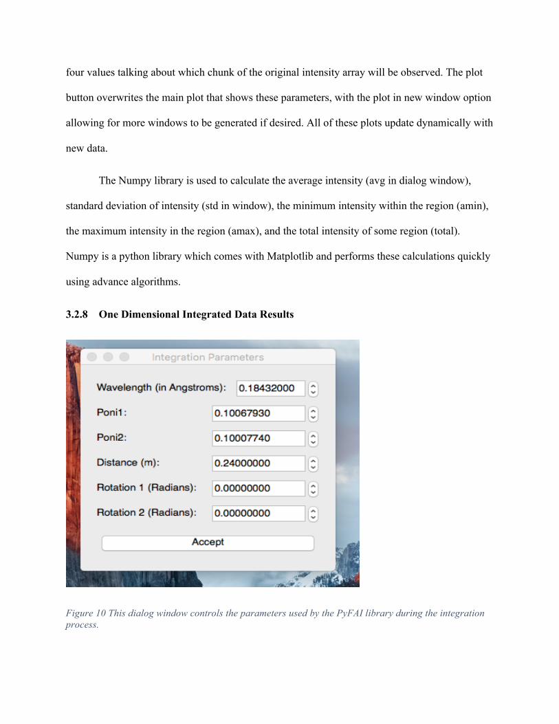
3.2.8 One Dimensional Integrated Data Results
Figure 10 This dialog window controls the parameters used by the PyFAI library during the integration process.

The integration used to create the one dimensional integrated reduced data plots comes
from the PyFAI library. The actual codes contain the specifics for how it is done, but the dialog
window shown in Figure 9 is where the user enters values to ensure that the integration takes all
factors into account desired by user.
The wavelength of the x-rays needs to be given in angstroms. Poni1 and Poni2 refer to
the point on the detector where the center of the patterns can be found. The distance, refers to the
distance from the detector to the sample. The two rotation values refer to how much the detector
is rotated in the XY plane and YZ plane directions.
3.3 Software Specifications
The software has been installed on the beam line and we have obtained optimal results.
Since there was no previous version of the software it is difficult to draw comparisons. One of
the main ways that success has been defined for this project has been the incorporation of the
features desired by the scientists. Many of the fundamental features such as viewing 2D
diffraction patterns and their corresponding 1D integrated patterns are now implemented. A
variety of other options are also now available to users of the software as are discussed in section
3.2.
The software was tested on a computer with an i7 processor at 2.9 Ghz that also had 8
GB of RAM. Images were read into the XPD View at a rate of three 2048x2048 pixel images
every second. Refreshing took the same amount of time. Redrawing the image, when diffracted
and integrated data are changed, took less than one tenth of a second. It took approximately half
of a second to draw the reduced representation, the top right quadrant, for when we looked at a
400x400 pixel area on the 2D diffracted data.

On beam line computers speed are even higher due to higher quality processors and
amount of RAM available to be used. No precise calculations were made, but the reading rate
was about five images every second or so.

4. Conclusion
As mentioned in the previous section, many of the original features have been implemented as
asked by beam line staff. The software was successfully installed on beam line computers and is
running at optimal speeds. The only thing that remains is to add more useful features.
Currently under development is the ability to stream live data from all the detectors and
meaningfully interpret the data to the many situations needed. The DAMA group has taken over
management of the software and will continue to lead the development to best help all the
scientists involved with these kinds of software. The beam line staff are in initial testing phases
to understand their needs and what else will be needed with the software to streamline the
experimenting and data analysis processes.

5. References
B Frandsen, Z Gong, M Terban, S Banerjee, B Chen, C Jin, M Feygenson, Y Uemura, S
Billinge, Local atomic and magnetic structure of dilute magnetic semiconductor (Ba,
K)(Zn, Mn)2As2, Phys. Rev. B: Condens. Matter, Early (2016).
D Sprouster, J Sinsheimer, E Dooryhee, S Ghose, P Wells, T Stan, N Almirall, G Odette, L
Ecker, Structural Characterization of Nanoscale Intermetallic Precipitates in Highly
Neutron Irradiated Reactor Pressure Vessel Steels, Scripta Mater., 113(1), 18-22 (2015).
Girolami, G. S. (2016). X-ray crystallography (1st ed.). Mill
Introduction to Matplotlib. (n.d.). Retrieved October 08, 2016, from http://matplotlib.org/
J Arinez-Soriano, J Jorge Albalad, A Carne-Sanchez, C Bonnet, F Busque, J Lorenzo, J
Juanhuix, M Terban, I Imaz, et al., pH-Responsive Relaxometric Behaviour of
Coordination Polymer Nanoparticles Made of a Gadolinium Macrocyclic Chelate, Chem.
Eur. J., 22(37), 13162-13170 (2016).
K Wang, A Wang, A Tomic, L Wang, A Abeykoon, E Dooryhee, S Billinge, C Petrovic,
Enhanced Thermoelectric Power and Electronic Correlations in RuSe2, APL Mater., 3(4),
041513 (2015). [107539]
L Wangoh, Y Huang, R Jezorek, A Kehoe, G Watson, F Omenya, N Quackenbush, N Chernova,
M Whittingham, L Piper, Correlating Lithium Hydroxyl Accumulation with Capacity
Retention in V2O5 aerogel cathodes, ACS Appl. Mater. Interfaces, 8(18), 11532-11538
(2016)

Materials Engineering. (n.d.). Retrieved December 04, 2016, from
http://www.substech.com/dokuwiki/doku.php?id=metals_crystal_structure
NumPy¶. (n.d.). Retrieved October 08, 2016, from http://www.numpy.org/
Page. (n.d.). Retrieved October 08, 2016, from https://wiki.python.org/moin/PyQt
PyFAI 0.8.8 : Python Package Index. (n.d.). Retrieved October 08, 2016, from
https://pypi.python.org/pypi/pyFAI/0.8.8
SciPy.org¶. (n.d.). Retrieved October 08, 2016, from http://www.scipy.org/
Tifffile 0.9.2 : Python Package Index. (n.d.). Retrieved October 08, 2016, from
https://pypi.python.org/pypi/tifffile
XpdView: Final Summer Release. (2016). Retrieved October 08, 2016, from
http://zenodo.org/record/60924
Why does the Debye-Scherrer procedure work (powder diffractometer). (n.d.). Retrieved
December 04, 2016, from http://physics.stackexchange.com/questions/92761/why-does-
the-debye-scherrer-procedure-work-powder-diffractometer