development of an extended exterior differential calculus · development of an extended exterior...
TRANSCRIPT
DEVELOPMENT OF AN EXTENDED EXTERIORDIFFERENTIAL CALCULUS
BY
HARLEY FLANDERS
Introduction
The purpose of this paper is to set up an algebraic machinery for the
theory of affine connections on differentiable manifolds and to demonstrate by
means of several applications the scope and convenience of this mechanism.
We shall associate with a manifold a series of spaces, best described as
spaces of multivectors with exterior differential form coefficients, and shall
exhibit the algebraic relations between these spaces. It is possible to consider,
in a more general fashion, spaces of tensors with differential form coefficients;
this is done, in fact, in Cartan [3, Chap. VIII, Sec. IlJC), where their use is
justified by means of geometrical considerations.
We shall define an affine connection as a certain kind of operator on the
space of ordinary vector fields to the space of vector fields with differential
one-form coefficients. It will be seen that this is simply another formulation
of the classical definition. One of our basic results (Theorem 7.1) is that an
affine connection induces an operator on each of the series of spaces just men-
tioned.
In Chapter I, we shall summarize the facts that we need about differenti-
able manifolds and introduce some notation. Chapter II is devoted to the
algebraic structure of the series of spaces Tpj that we introduce. In Chapter
III, we give the calculus associated with an affine connection and applications
to a number of identities. In the final chapter, we discuss some applications
of our calculus to Riemannian geometry, in particular to the "curvatura
integra" of S. Chern.
We hope in the future to give applications of this theory to other parts of
differential geometry, possibly to the theory of harmonic integrals and to the
theory of Lie groups.
Chapter I. Differentiable manifolds
1. Basic definitions. Let 2JÎ denote an M-dimensional differentiable mani-
fold. Usually we shall assume that 30Î is of class C°°, i.e., 592 bears an infinitely
differentiable structure; however, we shall have occasion for a few remarks
on the C" case, i.e., when 90? bears an analytic structure (Chevalley [9]).
The definitions and results we shall now state for Cx structures carry over
Presented to the Society, December 29, 1952; received by the editors August 25, 1952.
(') Numbers in brackets refer to the bibliography at the end of this paper.
311License or copyright restrictions may apply to redistribution; see http://www.ams.org/journal-terms-of-use
312 HARLEY FLANDERS [September
with slight modifications to the analytic case. The reader may consult
Chevalley, loc. cit., for details.
The Cx structure of 59? carries along with it a space C(90?) of all infinitely
differentiable real-valued functions on SO?. Let P be a point of 90?. A tangent
vector at P is a real-valued function v on C(Af) satisfying
(1) v(f+g) = v(f) + vig),
(2) v(af) = avif),
(3) vifg) = v(f)g(P) + f(P)v(g).
Here/, g£C(59?) and a is real. The set of all tangent vectors at P forms a
linear space which we shall denote by Xp. It is known that Xp is an «-dimen-
sional space and that a basis of Xp may be obtained as follows(2). Let U be a
local coordinate neighborhood on 59?, containing P, and with coordinate func-
tions x1, ■ ■ • , xn. Define vectors e, at P by e,(/) = (df/dxi)P. Then ei, • • • , e„
is a basis of Xp. The dual space %p of Xp is usually called the space of one-
Jorms at P. The basis of j$p which is dual to the basis ei, • ■ • , e„ is denoted
dxl, ■ ■ ■ , dxn. Thus if [v, w'] denotes the application of a one-form w'
to a vector v, then [e,-, dx1'] — 5}f, the Kronecker ô.
If v is any tangent vector at P, then v = 22aiei, with unique constants ai.
A mapping X which sends each point P of 59? into a tangent vector XiP) in
Xp is called a vector field (or infinitesmal transformation) provided that in each
local coordinate neighborhood IX the expression XiP) = 22ai(xl< ' ' ' > *n)e¿
defines C°° functions a'(x) on a region of euclidean space E„. When there is
no danger of confusion, we shall refer to such a vector field simply as a
vector on 59? and denote it by the same symbol v as we used for a vector at a
point. In the same manner we define a form field or differential form of degree
one, w= 22aidx'.The following notation will be useful. Let 70 = 70(90?) denote the ring of
all Cx functions on SO?. We have previously called this C(90?), but now wish
to include it in the hierarchy of ç-forms. Let 13 = 15(90?) be the space of all
vectors (i.e., vector fields) on 90?. This space may be considered as a linear
space over the ring of operators Jo (see Bourbaki [l]).
In much of this paper we shall work locally. Let U be a local coordinate
neighborhood of 59?. Then U is an open connected subset of 90? so that U itself
is an «-dimensional manifold. Thus all that has been said may be applied to
U. However the fact that U may be coordinatized implies the special prop-
erty that 13 is an «-dimensional space over the ring Jo.
2. Two important bundles. Consider the space $8i = Up£i>. This is a fiber
bundle (Steenrod [12]), called the tangent bundle of the manifold 90?, and it
again carries a C°° structure; in fact, from the expression v= ^a*e,- we ex-
(2) This result is given in Chevalley, loc. cit., for C" structures. Since it is not readily ac-
cessible as we have stated it, we shall include a short proof in the appendix to this chapter.
License or copyright restrictions may apply to redistribution; see http://www.ams.org/journal-terms-of-use
1953] AN EXTENDED EXTERIOR DIFFERENTIAL CALCULUS 313
tract the local coordinate system x1, • • ■ , xn, a1, • ■ • , an on the neighbor-
hood of 93i consisting of Upeuïp. A vector field on 59? is the same thing as a
C°° cross section of S8i.
Next, by a frame at P we mean any basis ei, • ■ ■ , e„ of the linear space
Xp. The set of all frames at all points P of 90? forms a new bundle 93„ called
the frame bundle of 90?. Since one passes from one frame to another in Xp by
the most general nonsingular linear transformation on an «-dimensional
linear space, it follows that Sß„ has dimension n+n2. A cross section of 33„ is
called a moving frame on 90?. The application of such frames to Riemannian
geometry has been given in Flanders [ll].
3. Multivectors and forms. Over the vector space Xp associated with a
point P of 59?, one may form the space /\pXp of /»-vectors at P. (See Cartan
[3, 4] and Bourbaki [2].) In the same way one may form the space /\9%p of
ç-forms at P. Each of these gives rise to a corresponding bundle (on which,
again, the full linear group acts), whose C°° cross sections are called p-vector
fields and differential form fields of degree q respectively.
It is important to note that the ring C(90?) acts both on the linear space
13p(90?) of all /»-vector fields and on the linear space 7,(90?) of all g-forms
(ç-form fields) on 59?. This remark helps to clarify the following assertion. Let
us restrict attention to a local coordinate neighborhood U on 90?, Jo = C(U) as
above, 15P = 13Î'(U), 7« = 7s(U). The space 13' = 15 is then an «-dimensional
space over 7o and it is true that 13p = A p13 formed over this coefficient domain
7o. In the same way Jq = A"Ji-4. Appendix. In this section we shall sketch a proof of the assertions in
§1 about the structure of the space Xp. The crux of the proof is contained in
the following lemma, whose proof was communicated to the author by Pro-
fessor H. F. Bohnenblust.
Lemma 4.1. Let fix) be a CM function defined in a neighborhood of 0 on the
real axis. Assume/(0) =0. Then there is a Cx function g(x) defined in the same
neighborhood such that g(x) =/(x)/x for x¿¿0 and g(0) =/'(0).
It should be noted that this is trivial for/(x) analytic, and it is this fact
which is used in Chevalley [9, p. 78] to prove the corresponding facts about
Xp in the case of analytic manifolds. To prove our lemma, we simply write
down the answer. Set
(4.1) gix) = f f'itx)dt.J o
This function is easily seen to have the required properties.
Corollary. Let Fix1, ■ ■ ■ , xn) be a C°° function in a star-shaped neighbor-
hood U of a point a = (a1, ■ • • , a") of En. Then there exist C°° j'unctions
G,(x) (t = l, • • • , «, x=(x1, • • • , xn)) on the same neighborhood such that
License or copyright restrictions may apply to redistribution; see http://www.ams.org/journal-terms-of-use
314 HARLEY FLANDERS [September
F(*) = ÜGiWtr-fl') and C(a) = (dF/dx*)«.
This is proved by applying the lemma to the function f(u)
= F(a+u(x — a)).
The proof of our assertions about Xp is now almost identical with that in
Chevalley, loc. cit., so we shall omit further details.
Chapter II. Vectors with form coefficients
5. Algebraic properties. In this section we shall consider the tensor prod-
ucts
(5.1) tfq = Jq®KP.
These spaces may be considered from two points of view: either as tensor
products of the spaces 7« and 15" over the ring 7o, or as cross sections of the
bundle of all elements of all (A q%p) <8> (A pXp) ; there the latter tensor product is
taken over the field of reals. At any rate, the ring 7o acts as a coefficient ring
for the spaces 13£.
Let us set 7= S®7a> e& = 22®^p- Each of these spaces is an algebra
over 7o, where multiplication is the Grassmann product. This implies, passing
to homogeneous components, the existence of an operation on 13jX13j' to
13¡+p given by linearity and
(5.2) (cov)(r,w) = (íoV)vw, where <o E Jq, n G J,', vG^.h-G 15"'.
This operation is associative and distributive, and obeys the following com-
mutation rule
(5.3) vw = (— 1) wv for v GE 13s and w Ç.15q'.
6. The displacement vector. Let ei, • • • , e„ be a moving frame on a local
coordinate neighborhood U of 90?. I.etcr1, • • • , <rn be a dual basis of one-forms.
We set
(6.1) dP = a1ei+ ■ ■ • + anen
so that dP£13l. It is clear that dP is intrinsic, i.e., it is independent of the
particular moving frame which is used to define it, and we shall call it the
displacement vector of 90?. The geometric meaning of dP is easily seen as fol-
lows (Cartan [3]). Let P = P(t) be a moving particle on 59?, where the real
variable t denotes time. Then along the trajectory c of P the ai contract to
one-forms in / and the velocity vector of P is given by
dP a1 an(6.2) —- = — ei +•••+— en.
dt dt dt
As examples of our multiplication we have
License or copyright restrictions may apply to redistribution; see http://www.ams.org/journal-terms-of-use
1953] AN EXTENDED EXTERIOR DIFFERENTIAL CALCULUS 315
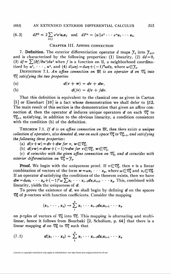
(6.3) dP2 = 2 22 o-^'eiej and dP" = (n?)al - ■ ■ «•"«, • • • e„.i<i
Chapter III. Affine connection
7. Definition. The exterior differentiation operator d maps Jq into 7«+i
and is characterized by the following properties: (1) linearity, (2) dd = 0,
(3) d/= 5Z(d//âM*)dM* when / is a function on U, a neighborhood coordina-
tized by ul, ■ ■ ■ , un, and (4) d(wrf) =dur) + ( — l)qœdr}, where wG7«-
Definition 7.1. An affine connection on 59? is an operator d on T5¿ into
13] satisfying the two properties
(a) d(v + w) = d v + dw,
(b) difv) = dfv + fdv.
That this definition is equivalent to the classical one as given in Cartan
[5] or Eisenhart [10] is a fact whose demonstration we shall defer to §12.
The main result of this section is the demonstration that given an affine con-
nection d, then the operator d induces unique operators d on each 13' to
13j+1 satisfying, in addition to the obvious linearity, a condition consistent
with the condition (b) of the definition.
Theorem 7.1. If d is an affine connection on 59?, then there exists a unique
collection of operators, also denoted d, one on each space 13£ to 13j+1, and satisfying
the following three properties:
(a) d(v + w) =dv + dwfor v, w£13j,
(b) d(vw) = dvw+(-l)"vdwfor v£13J, w£13sr,
(c) d coincides with the given affine connection on 15j, and d coincides with
exterior differentiation on ^5q=Jq-
Proof. We begin with the uniqueness proof. If v£13j, then v is a linear
combination of vectors of the form w=coxi • • • xp, where wG:13° and x¿GE 13o-
If an operator d satisfying the conditions of the theorem exists, then we have
dw = dwxi • • • xp + ( — l)*w ¿2xi ' ' ' xi-idx,Xi+i ■ ■ ■ xp. This, combined with
linearity, yields the uniqueness of d.
To prove the existence of d, we shall begin by defining d on the spaces
13J of /»-vectors with function coefficients. Consider the mapping
V
(xi, • ■ • , Xp) —» 22 xi " - - Xi-idx¿x,+i • • • xpi
on /»-tples of vectors of 13j into 13f. This mapping is alternating and multi-
linear, hence it follows from Bourbaki [2, Scholium, p. 64] that there is a
linear mapping d on 13o to 13Ï such that
(7.1) d(xi ■ ■ ■ xp) = 22 xi • • ■ Xi-iCiXiXi+i • • • Xpi
License or copyright restrictions may apply to redistribution; see http://www.ams.org/journal-terms-of-use

316 HARLEY FLANDERS [September
for any vectors xi, • • • , xp in 13j. To show that (b) is satisfied for v£13o,
w£13á, we observe that by linearity it suffices to consider the case v = xi ■ ■ •
Xp, w = yi ■ ■ ■ yr where the x,-and y,- are in 15¿. But property (b) is immediate
in view of the last formula.
We complete the proof by defining d on 13j. To do this, we consider the
mapping
(<o, v) —* dbiv + (— l)"wdv
which is on 13°X13S into 13J+1. This mapping is bilinear and so we may apply
the result in Bourbaki [2, Scholium, p. 7] to prove that there is a linear map-
ping d on T3J = 13J®13S into 13J+1 such that
(7.2) d(uv) = duv+ (- l)Wv
for any «£13° and any v£13o.
It now remains to verify property (b). By linearity, it suffices to do this
in the following special case: v=cou, w = r¡z, where w£13j, t?£13j, uGE15o,
*£135. In this case we have
d(vw) = d[(wu)(r¡z)] = d [(un) (uz)]
= d(ar,)(uz) + (- iy+>(m)d(uz)
= (dwr) + (- l)«wdij)(uz) + (- l)q+s(o>r\)(duz + udz)
= (dwu)(ijz) + (-l)»(wu)(dijz) + (-l)»(wdu)(ijz) + i-l)«+'iwu)iridz)
= (dcou + (- l)"o>du)(Vz) + (- l)"(ùiu)(dvz + i- l)'r¡dz)
= dvw + (— l)qvdw.
In this computation we have used the relation r]du = i — l)'dur]. This is a
consequence of the commutation rule (5.3).
We may now simplify our notation by using the same symbol d to denote
exterior differentiation d, the (given) affine connection d, and all of the
derived operators d of the last theorem.
8. Curvature and torsion. The following matrix notation will greatly
simplify our work. If ei, • ■ • , e„ is a moving frame with the dual basis of
forms a1, ■ • • , a", we shall set
(8.1) e = i '• J, a = (y • • • er»)
\e/
and we make the convention of identifying a 1X1 matrix with its single
element. Thus the equation (6.1) becomes
(8.2) dP = ae.
Henceforth let us assume that 59? is a manifold with an affine connection d.
License or copyright restrictions may apply to redistribution; see http://www.ams.org/journal-terms-of-use
1953] AN EXTENDED EXTERIOR DIFFERENTIAL CALCULUS 317
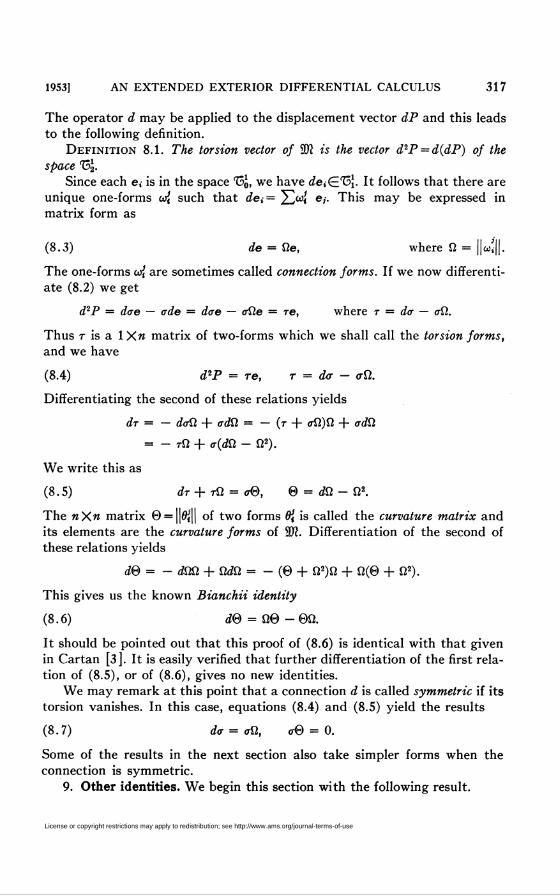
The operator d may be applied to the displacement vector dP and this leads
to the following definition.
Definition 8.1. The torsion vector of 90? is the vector d2P = d(dP) of the
space ^d\.
Since each e¿ is in the space 13j, we have deiG;13}. It follows that there are
unique one-forms co{ such that de,= 22œi ei- This may be expressed in
matrix form as
(8.3) de = Í2e, where Í2 = ||co¿||.
The one-forms co| are sometimes called connection forms. If we now differenti-
ate (8.2) we get
d2P = dae — ade — dae — aüe = re, where t = do — aü.
Thus t is a IX« matrix of two-forms which we shall call the torsion forms,
and we have
(8.4) d2P = re, r = der - <rfi.
Differentiating the second of these relations yields
dr = - daU + odti = — (r + ati)ti + odti
= - tO + <r(dü - Q2).
We write this as
(8.5) dr+TÜ = a&, 6 = dO - Ü2.
The «X« matrix © = ||ff{|| of two forms 0< is called the curvature matrix and
its elements are the curvature forms of 90?. Differentiation of the second of
these relations yields
d® = - dm + OdO = - (9 + tl2)Q + ß(0 + Ü2).
This gives us the known Bianchii identity
(8.6) d© = i20-0O.
It should be pointed out that this proof of (8.6) is identical with that given
in Cartan [3]. It is easily verified that further differentiation of the first rela-
tion of (8.5), or of (8.6), gives no new identities.
We may remark at this point that a connection d is called symmetric if its
torsion vanishes. In this case, equations (8.4) and (8.5) yield the results
(8.7) da = o-O, 0-9 = 0.
Some of the results in the next section also take simpler forms when the
connection is symmetric.
9. Other identities. We begin this section with the following result.
License or copyright restrictions may apply to redistribution; see http://www.ams.org/journal-terms-of-use
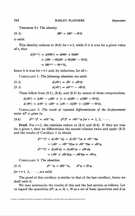
318 H ARLE Y FLANDERS [September
Theorem 9.1 The identity
(9.1) d9r = 09r - 9rO
is valid.
This identity reduces to (8.6) for r = 1, while if it is true for a given value
of r, then
d(9'+1) = d(99r) = d99' + 9d9'
= (09 - 90)9r + 9(09r - 9r0)
hence it is true for r + l and, by induction, for all r.
Corollary 1. The following identities are valid.
(9.2) d(o-9r) = r9r + 09--0.
(9.3) d(r9r) = o-9r+1 - r®rti.
These follow from (9.1), (8.4), and (8.5) by means of these computations.
d(o9r) = do®r - ad®' = (t + oti)®* - o(ti®r - ®'ti).
d(r9r) = dr®r + rd9r = (<r9 - t0)9' + t(09-- - 9r0).
Corollary 2. The result of repeated differentiation of the displacement
vector dP is given by
(9.4) d2r~lP = o®'-le, d2'P = r®'-lefor r = 1, 2, • • • .
Proof. For r = l, the relations reduce to (8.2) and (8.4). If they are true
for a given r, then we differentiate the second relation twice and apply (8.3)
and the results of Corollary 1 to obtain
d2r+ip = d(r®r-le) = d(r9'-1)e + r9'"1de
= (o®r - r9'~10)e + rQ^tie = o9re,
d2*+2P = d(o®re) = d(o®r)e - o®'de
= (r9r + <r9r0)e - a®rtie = r9re.
Corollary 3. The identities
(9.5) d2'~xe = 09r-1e, d2re = ®'e,
for r — \, 2, • • • , are valid.
The proof of this corollary is similar to that of the last corollary, hence we
shall omit it.
We may summarize the results of this and the last section as follows. Let
us regard the quantities dP, e, a, fl, r, 9 as a set of basic quantities and d as
License or copyright restrictions may apply to redistribution; see http://www.ams.org/journal-terms-of-use
1953] AN EXTENDED EXTERIOR DIFFERENTIAL CALCULUS 319
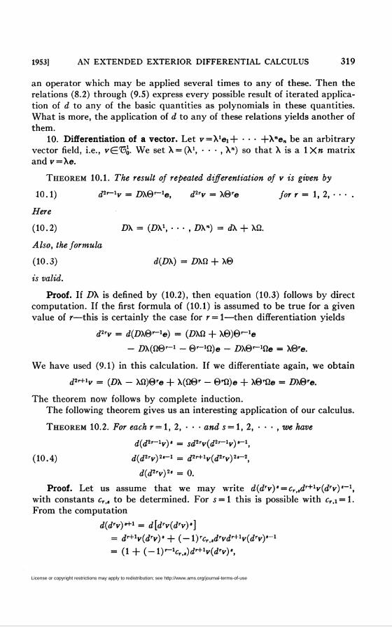
an operator which may be applied several times to any of these. Then the
relations (8.2) through (9.5) express every possible result of iterated applica-
tion of d to any of the basic quantities as polynomials in these quantities.
What is more, the application of d to any of these relations yields another of
them.
10. Differentiation of a vector. Let v=X1ei + • • • +X"e„ be an arbitrary
vector field, i.e., v£13¿. We set X=(XS • • • , X") so that X is a IX« matrix
and v = Xe.
Theorem 10.1. The result of repeated differentiation of v is given by
10.1) d2,-V = £>X9'-1e, d2rv = X9re for r = 1, 2, • • • .
Here
(10.2) D\ = (DX\ ■ ■ ■ , DX") = d\ + XO.
Also, the formula
(10.3) d(D\) = DX0 + X9
is valid.
Proof. If DX is defined by (10.2), then equation (10.3) follows by direct
computation. If the first formula of (10.1) is assumed to be true for a given
value of r—this is certainly the case for r = 1—then differentiation yields
d2rv = d(Z)X9r"1e) = (DXO + X9)9r-'e
- D\(ti®r~l - 9'-10)e - £»X9r-10e = X9re.
We have used (9.1) in this calculation. If we differentiate again, we obtain
¿2H-V = (£>x - X0)9re + X(09r - 9r0)e + X9r0e = Z?X9re.
The theorem now follows by complete induction.
The following theorem gives us an interesting application of our calculus.
Theorem 10.2. For each r= 1, 2, • • • and s = 1, 2, • • • , we have
d(d2*-lv)° = sd2rv(d2r-1v)a-\
(10.4) d(d2'v)2'-1 = d2*+lv(d2w)2*-2,
d(d2W)2> = 0.
Proof. Let us assume that we may write d(drv)s = cr,sdr+1v(drv)ä_1,
with constants cT,, to be determined. For 5=1 this is possible with cr,i=l.
From the computation
d(drv)'+1 = d[dwidrvY]
- dr+V(drv)9+ i-l)rCr,.drvdr+1vidrv)>-1
= ii + i-iy-hrjd^vid'vY,
License or copyright restrictions may apply to redistribution; see http://www.ams.org/journal-terms-of-use
320 HARLEY FLANDERS [September
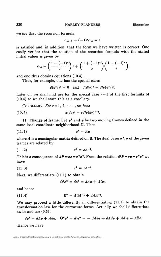
we see that the recursion formula
Cr,«+1 + (-l)rCr,„ = 1
is satisfied and, in addition, that the form we have written is correct. One
easily verifies that the solution of the recursion formula with the stated
initial values is given by
/l-(-l)'\ /l + (-l)'\/l-(-l)*\
*" = V-2-) S + v-2-) {—¥—) '
and one thus obtains equations (10.4).
Thus, for example, one has the special cases
did2v)2 = 0 and did2v)3 = d3v(dV)2.
Later on we shall find use for the special case r — 1 of the first formula of
(10.4) so we shall state this as a corollary.
Corollary. For r=l, 2, • • • , we have
(10.5) didvY = rd2vidvY-\
11. Change of frame. Let e* and e be two moving frames defined in the
same local coordinate neighborhood U. Then
(11.1) e* = Ae
where A is a nonsingular matrix defined on U. The dual bases a*, a of the given
frames are related by
(11.2) a* = oA-\
This is a consequence of dP = ae = a*e*. From the relation d2P = re = T*e* we
have
(11.3) r* = tA~K
Next, we differentiate (11.1) to obtain
0*e* = de* = dAe + Atie,
and hence
(11.4) ti* = AtiA-1 + dAA-1.
We may proceed a little differently in differentiating (11.1) to obtain the
transformation law for the curvature forms. Actually we shall differentiate
twice and use (9.5) :
de* - dAe + Ade, ®*e* = d2e* = - dAde + dAde + Ad2e = A®e.
Hence we have
License or copyright restrictions may apply to redistribution; see http://www.ams.org/journal-terms-of-use

1953] AN EXTENDED EXTERIOR DIFFERENTIAL CALCULUS 321
(11.5) 9* = A®A-\
Next, let v = Xe be a vector field. Then dv = Z)Xe = Z)X*e*, hence
(11.6) D\* = D\A-\
12. Classical formulation. For the sake of completeness, we shall indicate
here how the quantities we have introduced may be expressed in the language
of the tensor calculus. In this section we shall use the Einstein summation
convention whereby common upper and lower indices are summed.
The one-forms otf may be expressed in terms of the basis ok of one-forms
according to
(12.1) «,' = VihoK
This defines the connection coefficients T,'* relative to the given moving frame
e. Similarly we may write
(12.2) 6i' = 2-1Ri>kiohol with JKi'm + Ri'u = 0,
(12.3) r* = 2-lTijko'ok with ¡T'ji + T<kj = 0,
(12.4) D\< = XV.
These equations define the Riemann tensor Ri'ki, the torsion tensor T{¡k,
and the covariant derivative X',y of X'. That each of these quantities actually
satisfies the tensor transformation law is a consequence of the equations of
the last section. Each of our identities may be expressed as an identity in-
volving the tensors defined in the last four equations.
It is now easy to show that our Definition 7.1 of an affine connection is
equivalent to the usual one. We first of all specialize our formulas to the case
in which the vectors ei, ■ • • , e„ of the moving frame are directional differen-
tiations with respect to coordinate functions. Thus let x1, • • • , x" be a local
coordinate system and let
d d(12.5) d =-j • • • j e„ = -•
dx1 dxn
Then by (6.1) we have
(12.6) dP = dx'ei + • • • + dxne„,
which is to say that ai = dxi, and so to¿J'= IYidx*. It follows that
(12.7) dei = Ti>\dxkej.
Corresponding to each frame (12.5) we thus have functions IV*. To find their
transformation law, we let x*, • • ■ , x* be another local coordinate system
and e* the corresponding frame. Then (11.1) is valid, where A is the Jacobian
matrix
License or copyright restrictions may apply to redistribution; see http://www.ams.org/journal-terms-of-use
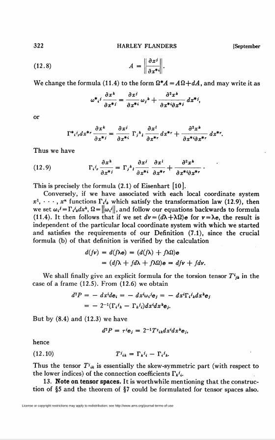
322 HARLEY FLANDERS [September
(12.8)dx'
dx*1
We change the formula (11.4) to the form tl*A =AQ,+dA, and may write it as
dxk dx'
dx*' dx*i<*ik +
d2xk
dx*idx*>- dx*>;
or
T*i'rdx*r ■dxk
dx*'
dx' dx1Yikl—-dx*r +
d2xk
dx
Thus we have
(12.9)dxk
dx*'
dx*
dx' dx1
dx*idx*rdx*
1 » r _ ... . í l I . ^, . ^
d2Xk
dx** dx*r dx^dx**
This is precisely the formula (2.1) of Eisenhart [lO].
Conversely, if we have associated with each local coordinate system
x1, • • • , x" functions l'A which satisfy the transformation law (12.9), then
we set Ui' = Ti'kdxk, Í2 = ||w¿'||, and follow our equations backwards to formula
(11.4). It then follows that if we set dv=(dX+Xß)e for v=Xe, the result is
independent of the particular local coordinate system with which we started
and satisfies the requirements of our Definition (7.1), since the crucial
formula (b) of that definition is verified by the calculation
difv) = d(/Xe) = (d(/X) + /XO)e
= (d/X + fd\ + /XO)e = dfv + fdv.
We shall finally give an explicit formula for the torsion tensor T'jk in the
case of a frame (12.5). From (12.6) we obtain
d2P = — dx^ei = — dx'ui'ej = — dxiYi'kdxkej
= - 2~liYJk - Yk'i)dxidxkei.
But by (8.4) and (12.3) we have
d2P = r'ej = 2~1T'ikdxidxkej,
hence
(12.10) T'ik = iVi - iy*.
Thus the tensor T'ik is essentially the skew-symmetric part (with respect to
the lower indices) of the connection coefficients IV,-.
13. Note on tensor spaces. It is worthwhile mentioning that the construc-
tion of §5 and the theorem of §7 could be formulated for tensor spaces also.
License or copyright restrictions may apply to redistribution; see http://www.ams.org/journal-terms-of-use
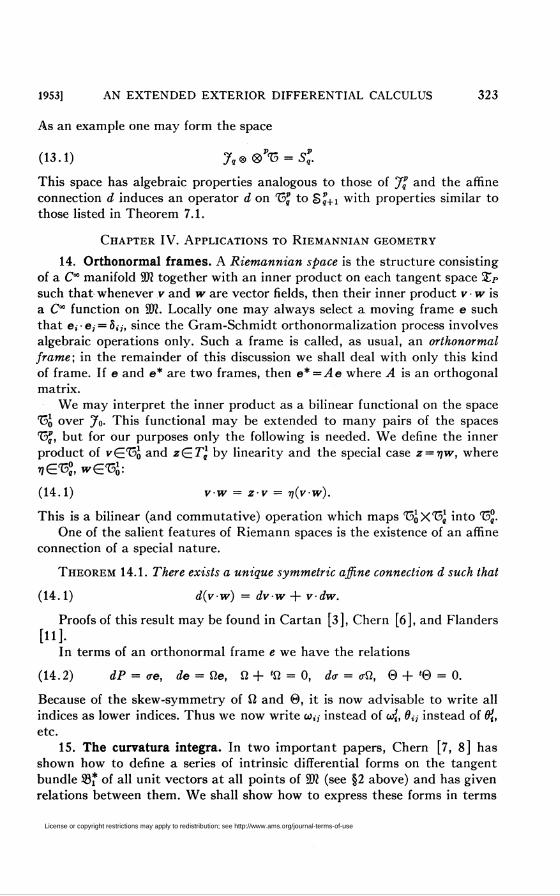
1953] AN EXTENDED EXTERIOR DIFFERENTIAL CALCULUS 323
As an example one may form the space
(13.1) Jq®®PK = SPq.
This space has algebraic properties analogous to those of 7« and the affine
connection d induces an operator d on 13^ to S^+i with properties similar to
those listed in Theorem 7.1.
Chapter IV. Applications to Riemannian geometry
14. Orthonormal frames. A Riemannian space is the structure consisting
of a Cx manifold 90? together with an inner product on each tangent space Xp
such that whenever v and w are vector fields, then their inner product v ■ w is
a Cx function on 90?. Locally one may always select a moving frame e such
that e¿-e, = 5,„ since the Gram-Schmidt orthonormalization process involves
algebraic operations only. Such a frame is called, as usual, an orthonormal
frame; in the remainder of this discussion we shall deal with only this kind
of frame. If e and e* are two frames, then e*=Ae where A is an orthogonal
matrix.
We may interpret the inner product as a bilinear functional on the space
13j over 7o- This functional may be extended to many pairs of the spaces
13j, but for our purposes only the following is needed. We define the inner
product of v£13¿ and z£7^ by linearity and the special case z = r)w, where
n £13?, w£13j:
(14.1) vw = zv = riiv-w).
This is a bilinear (and commutative) operation which maps 13¿X13J into 13°.
One of the salient features of Riemann spaces is the existence of an affine
connection of a special nature.
Theorem 14.1. There exists a unique symmetric affine connection d such that
(14.1) divw) = dvw + vdw.
Proofs of this result may be found in Cartan [3], Chern [6], and Flanders
[11].In terms of an orthonormal frame e we have the relations
(14.2) dP = ae, de = tie, 0 + <0 = 0, da = ati, 9 + '9 = 0.
Because of the skew-symmetry of ß and 9, it is now advisable to write all
indices as lower indices. Thus we now write co¿¡ instead of cojt, da instead of 6{,
etc.
15. The curvatura integra. In two important papers, Chern [7, 8] has
shown how to define a series of intrinsic differential forms on the tangent
bundle 93* of all unit vectors at all points of 59? (see §2 above) and has given
relations between them. We shall show how to express these forms in terms
License or copyright restrictions may apply to redistribution; see http://www.ams.org/journal-terms-of-use
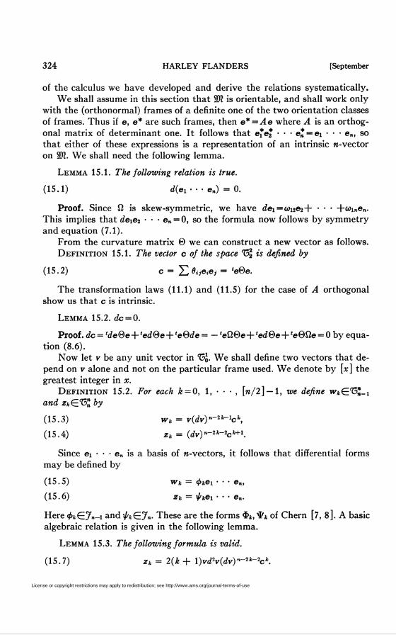
324 HARLEY FLANDERS [September
of the calculus we have developed and derive the relations systematically.
We shall assume in this section that 59? is orientable, and shall work only
with the (orthonormal) frames of a definite one of the two orientation classes
of frames. Thus if e, e* are such frames, then e*=^4e where A is an orthog-
onal matrix of determinant one. It follows that e*e* • • • e* = ei • ■ • e„, so
that either of these expressions is a representation of an intrinsic «-vector
on 90?. We shall need the following lemma.
Lemma 15.1. The following relation is true.
(15.1) d(ei- • • e„) = 0.
Proof. Since ß is skew-symmetric, we have dei=wi2e2+ ' • ■ +Wi„en.
This implies that deie2 ■ • • e„ = 0, so the formula now follows by symmetry
and equation (7.1).
From the curvature matrix 9 we can construct a new vector as follows.
Definition 15.1. The vector c of the space 13^ is defined by
(15.2) c = 22 9ii*i6j = 'e9e.
The transformation laws (11.1) and (11.5) for the case of A orthogonal
show us that c is intrinsic.
Lemma 15.2. dc = 0.
Proof. dc=íde9e + 'ed9e + íe9de= -ieß9e + 'ed9e + 'e9ße = 0 by equa-
tion (8.6).
Now let v be any unit vector in 13j. We shall define two vectors that de-
pend on v alone and not on the particular frame used. We denote by [x] the
greatest integer in x.
Definition 15.2. For each k = 0, 1, • • • , [n/2] — 1, we define w*£13"_1
and zkÇ.T5" by
(15.3) wk = vidv)n-2k-1ck,
(15.4) zk = idv)"-2k-2ck+1.
Since ei • • • e„ is a basis of «-vectors, it follows that differential forms
may be defined by
(15.5) wk = «Hei • ■ • e„,
(15.6) zk = ^ei • ■ • e„.
Here <pk(E.Jn~i and ^¿£7»- These are the forms €>*, ̂k of Chern [7, 8]. A basic
algebraic relation is given in the following lemma.
Lemma 15.3. The following formula is valid.
(15.7) Zk = 2(¿ + l)vdV(dv)''-2*-2cfc.
License or copyright restrictions may apply to redistribution; see http://www.ams.org/journal-terms-of-use
1953] AN EXTENDED EXTERIOR DIFFERENTIAL CALCULUS 325
Proof. Since v is a unit vector field, we may select a moving frame e in
such a way that ei = v. Since both members of (15.7) are intrinsic, we may
use this particular frame in the proof. By the second equation (9.5) with
r=l, we have d2e=9e, hence dV = d2ei= ¿2ßu ei< where the sum is taken
over j = 2, 3, • • • , «, since 9 is skew-symmetric. On the other hand, we have
c = 2-j Oiidej = 2-1 9ijeie¡ + ¿^ 0»ie,-ei + 2-, Oije,ej¡JÏ2
= 2ex 2_-0ij'eJ + 22^aeiei'
hence c = 2vd2v+h, where h is a vector of 132 which involves only e2, • • • , e„.
Since v2 = 0 and h commutes with every vector, we have
c* = 2kvd2vhk~1 + hk and ck+1 = 2<* + l)vd2vh* + hk+1
by the binomial expansion. Next, we assert that
idv)"-2k-2hk+1 = 0.
This is the case because dv = dei = 22iä2 Wi/«íi and so the vector on the left-
hand side is an «-vector in the (« — 1) vectors e2, • • • , e„, and hence vanishes.
Noting that vd2v is in "T^, and so commutes with every vector, we have
zk = (dv)"-2*-2c*+1
= 2(* + l)vd2vidv)n~2k-2hk
= 2(4 + l)vd2v(dv)"-2*-2c*.
The last equality is a consequence of the formula above for ck and the fact
thatv2 = 0.
The following result can be read out of the last proof.
Lemma 15.4. // v is a unit vector field, then (dv)n = 0.
For if v = ei, then dv=o)i2e2 + • • • -f-wi„e„, hence (dv)n is an «-vector in
e2, ■ ■ ■ , en.
It is convenient to set \p-i = 0 and z_i = 0. We now have our main result.
Theorem 15.1. For each k = 0, 1, • • • , [n/2] — l, we have
n — 2k — 1(15.8) dwk = Zfc_i H-Zk.
2ik+ 1)
Proof. We compute dwk from the formula (15.3), making use of equation
(10.5) and Lemma 15.2.
dwk = idv)"-2kck + in - 2k - l)vd2vidv)n-2k-2ck.
The first term is z*_i. This is the case by virtue of (15.4) when &>0, and by
Lemma 15.4 when £ = 0. The second term is equal to the last term of (15.8)
License or copyright restrictions may apply to redistribution; see http://www.ams.org/journal-terms-of-use

326 HARLEY FLANDERS
by Lemma 15.3.
Corollary 15.1. For k = 0, 1, • • ■ , [w/2] — 1, we have
« — 2k — 1(15.9) dft = ft-i + ft.
2(* + 1)
This result now follows from (15.5), (15.6), and Lemma 15.4.
Bibliography
1. N. Bourbaki, Algebre linéaire, Paris, 1947.
2. -, Algèbre multilinêaire, Paris, 1948.
3. E. Cartan, Leçons sur la géométrie des espaces de Riemann, Paris, 1928 (2d éd. 1946).
4. -, Les systèmes différentiels extérieurs et leurs applications géométriques, Paris, 1945.
5. -, Sur les variétés d connexion affine et la théorie de la relativité généralisée, Ann.
École Norm. (3) vol. 40 (1923) pp. 325-412.6. S. S. Chern, Some new viewpoints in differential geometry in the large, Bull. Amer. Math.
Soc. vol. 52 (1946) pp. 1-30.7. -, A simple intrinsic proof of the Gauss-Bonnet formula for closed Riemannian
manifolds, Ann. of Math. vol. 45 (1944) pp. 747-752.8. -, On the curvatura integra in a Riemannian manifold, Ann. of Math. vol. 46 (1945)
pp. 647-684.9. C. Chevalley, Theory of Lie groups, Princeton, 1946.
10. L. P. Eisenhart, Non-Riemannian geometry, New York, 1927.
11. H. Flanders, A method of general linear frames in Riemannian geometry, I, to appear
in the Pacific Journal of Mathematics.
12. N. Steenrod, The topology of fibre bundles, Princeton, 1951.
The University of California,
Berkeley, Calif.
License or copyright restrictions may apply to redistribution; see http://www.ams.org/journal-terms-of-use