development and evaluation of system restoration ... · of system restoration strategies from a...

Development and Evaluationof System Restoration Strategies

from a Blackout

Final Project Report

Power Systems Engineering Research Center

A National Science FoundationIndustry/University Cooperative Research Center

since 1996

PSERC

Development and Evaluation of System Restoration Strategies from a Blackout

Final Project Report

Project Team

Faculty: Chen-Ching Liu, Project Leader, University College Dublin

and Iowa State University Vijay Vittal, Gerald T. Heydt

Arizona State University Kevin Tomsovic, University of Tennessee

and Washington State University

Students: Wei Sun, Iowa State University

Chong Wang, Raul Perez, Torrey Graf, Benjamin Wells Arizona State University Benyamin Moradzadeh University of Tennessee

Hui Yuan Washington State University

PSERC Publication 09-08

September 2009

Information about this project For information about this project contact: Professor Chen-Ching Liu School of Electrical, Electronic and Mechanical Engineering University College Dublin National University of Ireland, Dublin Belfield Dublin 4, Ireland Phone: 353-1-716-1676 Email: [email protected] Power Systems Engineering Research Center The Power Systems Engineering Research Center (PSERC) is a multi-university Center conducting research on challenges facing the electric power industry and educating the next generation of power engineers. More information about PSERC can be found at the Center’s website: http://www.pserc.org. For additional information, contact: Power Systems Engineering Research Center Arizona State University 577 Engineering Research Center Tempe, Arizona 85287-5706 Phone: 480-965-1643 Fax: 480-965-0745 Notice Concerning Copyright Material PSERC members are given permission to copy without fee all or part of this publication for internal use if appropriate attribution is given to this document as the source material. This report is available for downloading from the PSERC website.

2009 Iowa State University, Arizona State University, and University of Tennessee. All rights reserved.

Acknowledgements

This is the final report for the Power Systems Engineering Research Center (PSERC) research project S-30 titled “Development and Evaluation of System Restoration Strategies from a Blackout”. We express our appreciation for the support provided by PSERC’s industrial members and by the National Science Foundation under grant NSF EEC-0001880 received under the Industry / University Cooperative Research Center program.

We wish to thank the industry advisors for their technical advice on this project: Larry Anderson (AEP), Frank Zhang (AEP), Jiangzhong Tong (PJM), Jinan Huang (Hydro Quebec), Thiru Venganti (ITC), Randy Ezzell (ITC), Achisman Gupta (ITC), Brian Keel (SRP), Armindo Castelhano (SRP), and Nevida Jack (SRP). We thank Floyd Galvan, Sharma Kolluri and Sujit Mandal from Entergy Corp. for their assistance during the research progress, especially for the Entergy system data and technical support. We are also grateful to Mike Adibi and Dr. Ron Chu, PECO-Energy for their valuable suggestions and contributions to this work.

This project involved the participation of some PSERC member companies: American Electric Power (AEP) Corporation, PJM Interconnection LLC, Entergy Corporation, Hydro-Québec Corporation, and ITC, who provided supplemental funding for the project and the associated data, and participated as an industry advisor to the project.

ii

Executive Summary

System restoration following a blackout is one of the most important tasks for power system operators. However, few on-line computer tools are available to help operators complete that task in real-time. Indeed, most power system operators rely on off-line restoration plans developed for selected scenarios of contingencies, equipment outages, and available resources. Since the details of an actual blackout are hard to predict in the planning stage, a restoration plan can only serve as a guide in an actual system restoration situation.

In this research, we used novel approaches to transmission and distribution system restoration to design modules that can be used in an on-line decision support tool. Using such a tool, once fully developed and tested, operators will be better able to adapt to changing system conditions that occur during an actual restoration. The research-grade modules include:

• Generation Capability Optimization Module

• Transmission Path Search Module

• Constraint Checking Module

• Distribution System Restoration Module. With additional development work, these modules could be linked and coordinated by a Strategy Module. Testing demonstrated the viability of these modules in identifying restoration decisions that we believe will reduce restoration time while maintaining system integrity. Ultimately, this will lead to lower outage costs for blackout events.

The four developed modules provide an automated and “best adaptive strategy” procedure for power system restoration. Future work will be needed for extensive testing, implementation planning, and actual implementation in a real-time operational environment.

Part I. Optimal Generator Start-up Strategies for Power System Restoration (work done at Iowa State University)

During system restoration, generation availability is fundamental for all stages of system restoration: stabilizing the system, establishing the transmission path, and picking up load. The generator start-up strategy is intended to provide an initial starting sequence of all black start or non-black start units. Available black start units must provide cranking power to non-black start units in such a way that the overall available generation capability is maximized. The corresponding generation optimization problem is combinatorial with complex practical constraints that vary with time. Two methods were developed and demonstrated for a Generation Capability Optimization Module.

First, by taking advantage of the quasiconcave property of generation ramping curves, a two-step algorithm was used for the generator start-up sequencing problem. The optimization problem was formulated as a Mixed Integer Quadratically Constrained Program (MIQCP). The solution method breaks the restoration horizon into intervals and develops the restoration plan by finding the status of each generator during each time

iii

interval. Optimality is achieved for each step individually. The algorithm was tested using PECO data.

Second, we derived a new formulation of the generator start-up sequencing problem as a Mixed Integer Linear Programming (MILP). The linear formulation leads to a global optimal solution that outperforms other heuristic or enumerative techniques in both quality of solution and computational speed. The IEEE 39-Bus system was used for validation of the generation capability optimization. The simulation results demonstrated the high efficiency of the MILP-based generator start-up sequencing algorithm.

Part II. Transmission System Restoration with Constraints Checking (work done at Arizona State University)

A Constraint Checking Module is needed for a restoration computer tool. After a system blackout, parallel restoration of subsections of the system is an efficient way to speed up restoration. The system sectionalizing strategy determines the proper splitting point to sectionalize the entire blackout area into several subsystems. Parallel restoration can be carried out in each subsystem. For a large scale power system, this system sectionalizing problem is complicated due to black start and generation/load balance constraints. For system sectionalizing, we used an ordered binary decision diagram method that quickly finds the splitting points. Simulation results on the IEEE 39-Bus system showed that the method successfully sectionalized the system in a way that satisfied the two constraints. The method was implemented in the Constraint Checking Module.

A Transmission Path Search Module enabled optimization of the restoration sequence for linking the subsystems into a larger system, thereby gradually reducing the number of subsystems to zero. An objective transmission restoration path selection procedure, with the option to check constraints, may be better able to handle unexpected system changes during restoration and still provide the information needed by system operators for completing the restoration process. We developed a path selection approach that used power transfer distribution factors (PTDFs) for large-scale power systems. Two types of restoration performance indices were computed. They included all possible restoration paths. The computed indices were ranked, then PTDFs and weighting factors were used to determine the ordered list of restoration paths. This method enabled load to be picked up by lightly-loaded lines or by relieving stress on heavily-loaded lines. Successful test results of the Transmission Path Search and Constraint Checking Modules were obtained by using the IEEE 39-Bus system and by doing a realistic restoration exercise for the western region of Entergy’s transmission system.

Part III. Automated Restoration of Power Distribution Systems (work done at Arizona State University and University of Tennessee)

During a system-wide restoration process, distribution system restoration is a critical task to help reduce economic losses and public dissatisfaction brought by a service interruption, especially in restructured competitive electricity markets. In this project we showed that fast, practical computational tools can be used to provide guidance for a distribution system restoration process that adapts to real-time system conditions. The tool can support decisions by operators during the restoration process by providing

iv

customized plans for specific system conditions. This form of automated (or, alternatively, semi-automated) tool is expected to run in parallel with the restoration process, with each run using updated values for loads and expected generation in order for the tool to use the best available information during the entire process.

The computer tool for the operator permissive distribution system automation approach used optimization algorithms, in particular, the Lagrangian relaxation method and Binary Integer Programming. Using the tool, restoration plans are developed using the objective of minimizing outage cost and restoration time for a specified percentage of system load restoration. Other objectives that consider a weighted priority ranking or system security may also be adopted by replacing the cost function with the pertinent objective function. Due to the dual characteristics of the Lagrangian relaxation method, global convergence is not guaranteed as some constraints may be ignored during the optimization problem. In addition, the total accuracy of the solution will also depend on the estimates used for load and expected available generation. Matlab codes for the Distribution System Restoration Module are given in the report.

The developed algorithms were tested on 4-feeder and 100-feeder test systems under several blackout scenarios. The results showed that automated restoration is practical for small and modest size systems (e.g., to at least 100 feeders and 25 substations). The tool is expected to reduce restoration times significantly. The number of hours per year required for restoration depends on the specific nature of the given distribution system. However, a system with system average interruption duration of three hours per year, for example, could be reduced to two hours per year. Networked distribution systems have the potential for dramatic reduction in system average interruption duration per year (e.g., by an order of magnitude).

Future work related to the distribution system restoration problem will enhance the models used in the tool to fully represent a practical restoration plan for a distribution system. Some needs for future development include:

• Further modeling of the cold load pick up phenomena

• Evaluation of the impact of phase sequence in capacitor switching

• Evaluation of the effect of system transmission and system voltage profile constraints in the distribution system restoration problem

• Determination of the role and candidacy of this tool as part of smart grid initiatives

• Development of demonstration projects for automated restoration

• Additional system configurations and various system constraints.

v

Part IV. Automated Optimal Transmission System Restoration (work done at Washington State University and University of Tennessee)

Transmission system restoration is critical to the integrated power system restoration process. It builds the transmission line skeleton to facilitate the restoration of generation and the distribution system. Generation units rely on this skeleton to pick up appropriate amount of loads to maintain a viable balance during restoration. Distribution substations rely on this skeleton to restore lost loads. The corresponding optimization problem is of combinatorial nature. The restoration algorithms assist system operators during restoration by determining the order and time at which transmission lines should be energized.

The optimal transmission path search is formulated into a Mixed Integer Quadratically Constrained Programming (MIQCP) problem under the assumption that the transmission network is lossless. Since the quadratic terms in the MIQCP problem are all pseudo (i.e., they are multiplication between a binary variable and a real number), a general rule is derived and proved to linearize these pseudo-quadratic terms. With the linearization of these pseudo-quadratic constraints, the MIQCP problem is converted to a Mixed Integer Linear Programming (MILP) problem. With the assistance of other more detailed analysis programs, the feasibility of a transmission line restoration plan can be checked. Any necessary adjustments can then be performed to satisfy all system constraints, static or dynamic.

The main contributions of this research are:

• Novel approaches for determining proper transmission system restoration strategies. • Formulation of the optimal transmission path search as an MILP problem. • Formulation and proof of a standard rule to linearize a pseudo-quadratic term.

This work constitutes an extension to transmission system restoration that was described in Part II. The viability of this approach was demonstrated on a 6-bus system.

vi

Table of Contents Part I. Optimal Generator Start-Up Strategy for Power System Restoration ....... 1

1.1 Introduction ................................................................................................................. 2

1.1.1 Background ........................................................................................................ 2

1.1.2 Restoration Procedure ........................................................................................ 3

1.1.3 Generator Start-up Sequencing Problem ............................................................ 4

1.1.4 Report Organization ........................................................................................... 5

1.2 "Two-Step" Generator Start-up Algorithm ................................................................. 6

1.2.1 Quasiconcavity ................................................................................................... 6

1.2.1.1 Definition of Quasiconcavity ...................................................................... 6

1.2.1.2 Lemma 1 ..................................................................................................... 6

1.2.2 “Two-Step” Generation Capability Curve ......................................................... 6

1.2.3 Algorithm ........................................................................................................... 7

1.2.4 Problem Formulation .......................................................................................... 7

1.2.4.1 Objective Function ...................................................................................... 7

1.2.4.2 Constraints .................................................................................................. 8

1.2.5 Flow Chart of the Algorithm ............................................................................ 10

1.3 MILP Based Generator Start-up Strategy ................................................................. 11

1.3.1 Problem Formulation ........................................................................................ 11

1.3.1.1 Objective Function .................................................................................... 11

1.3.1.2 Constraints ................................................................................................ 11

1.3.2 Algorithm ......................................................................................................... 15

1.3.3 Flow Chart of the Algorithm ............................................................................ 16

1.3.4 Illustration of Other Modules ........................................................................... 17

1.3.4.1 Transmission Path Search ......................................................................... 17

1.3.4.1.1 Correlation Matrix of Circuit Breaker (CB) and Busbar/line ............... 17 1.3.4.1.2 Shortest Path Solver ............................................................................. 17 1.3.4.1.3 Algorithm ............................................................................................. 19 1.3.4.1.4 Flow Chart ............................................................................................ 20

1.3.4.2 Constraint Checking.................................................................................. 20

1.3.4.3 Strategy Module ........................................................................................ 21

1.4 Numerical Results ..................................................................................................... 23

1.4.1 Case of Four-generator System ........................................................................ 23

1.4.2 Case of PECO System ...................................................................................... 25

1.4.3 Case of IEEE 39-Bus System ........................................................................... 28

1.4.4 Case of Western Entergy Region ..................................................................... 36

1.4.5 Performance Analysis of MILP Method .......................................................... 37

1.4.6 Comparison with Other Methods ..................................................................... 37

1.5 Conclusions ............................................................................................................... 38

vii

Table of Contents (continued)

Part II. Transmission System Restoration with Constraints Checking ................ 39

2.1 Introduction ............................................................................................................... 40

2.1.1 Background ...................................................................................................... 40

2.1.2 Overview of the Problem ................................................................................. 40

2.1.3 Report Organization ......................................................................................... 41

2.2 OBDD-Based System Sectionalizing Strategy .......................................................... 42

2.2.1 Ordered Binary Decision Diagram Model in Power System ........................... 42

2.2.2 Ordering of Branches and NP-Complete Solution ........................................... 45

2.2.3 Operating Condition and Simulation Result .................................................... 46

2.3 PTDF-Based Automatic Restoration Path Selection ................................................. 49

2.3.1 Introduction ...................................................................................................... 49

2.3.2 PTDF-Based Restoration Path Selection .......................................................... 49

2.3.2.1 Radial Lines Restoration Performance Index ........................................... 49

2.3.2.2 Loop Closure Lines Restoration Performance Index ................................ 51

2.3.2.3 N-1 Criterion and Area Determination Algorithm .................................... 52

2.3.2.4 Line Switching Issues ............................................................................... 54

2.4 Simulation Results ..................................................................................................... 55

2.4.1 June 15, 2005 Storm Case in Entergy System .................................................. 55

2.4.1.1 Introduction ............................................................................................... 55

2.4.1.2 Proposed System Restoration ................................................................... 57

2.4.2 Illustrations of Intermediate Steps .................................................................... 63

2.4.2.1 Example I: Radial Line Ranking with Type 1 RPI ................................... 63

2.4.2.2 Example II: Loop Closure Line Ranking with Type II RPI ...................... 65

2.4.2.3 Example III: Sustained Overvoltage Checking and Control ..................... 66

2.4.2.4 Example IV: Load Level Determination after Area I is Fully Restored ... 68

2.4.3 IEEE-39 Bus System Case ............................................................................... 68

2.5 Conclusions ............................................................................................................... 71

Part III. Automated Restoration of Power Distribution Systems .......................... 72

3.1 An Introduction to Power System Restoration .......................................................... 73

3.1.1 The Restoration Process ................................................................................... 73

3.1.2 This PSerc Project ............................................................................................ 73

3.1.3 An Introduction to Power System Restoration ................................................. 73

3.1.4 Objectives ......................................................................................................... 74

3.1.5 Literature Review ............................................................................................. 75

viii


3.1.5.1 Bulk Power System Restoration Issues..................................................... 75

3.1.5.2 Distribution System Restoration ............................................................... 78

3.1.6 Report Organization ......................................................................................... 78

3.2 Distribution System Restoration ............................................................................... 80

3.2.1 Load Restoration as Seen from the Primary of Distribution Systems .............. 80

3.2.2 The Distribution System Restoration Problem Formulation ............................ 81

3.2.2.1 The DSR Objective ................................................................................... 81

3.2.2.2 Constraints ................................................................................................ 84

3.2.3 DSR Formulation for Integer Programming .................................................... 85

3.2.4 Cold Load Pickup in Distribution System Restoration .................................... 87

3.2.4.1 Loss of Load Diversity .............................................................................. 88

3.2.4.2 Inherent Transient Behavior ..................................................................... 89

3.2.4.3 Load Uncertainty ...................................................................................... 90

3.2.4.4 CLPU Modeling ........................................................................................ 91

3.2.5 Unit Commitment and Distribution Restoration Duality ................................. 93

3.2.5.1 Key Parameters in the UC and DSR Problems ......................................... 94

3.2.5.2 Solution Methods ...................................................................................... 95

3.3 Lagrangian Relaxation Based Distribution Restoration ............................................ 97

3.3.1 Relaxations, Duality and Lagrangian Relaxation ............................................. 97

3.3.2 LR Based Distribution System Restoration ...................................................... 99

3.3.2.1 The Outer Problem and the Subgradient Iteration Method ..................... 100

3.3.2.2 The Inner Problem and the Restoration Index ........................................ 102

3.3.3 Distribution Restoration Infrastructure .......................................................... 103

3.3.4 An Evolutionary Computation Heuristic for the Outer Problem ................... 105

3.3.4.1 The Differential Evolution Optimization Algorithm .............................. 106

3.3.4.2 The Differential Evolution Optimization Process ................................... 106

3.3.5 Summary ........................................................................................................ 109

3.4 Binary Integer Programming Based Distribution Restoration ................................ 110

3.4.1 Problem Formulation ...................................................................................... 110

3.4.1.1 Maximize the Total Restored Weighted Energy ..................................... 110

3.4.1.2 Restore a Specified Percentage of System Load in the Shortest Time ... 112

3.4.2 Summary ........................................................................................................ 116

3.5 Illustrative Examples and Results ........................................................................... 117

3.5.1 Overview of Examples and Test Beds ........................................................... 117

3.5.2 Test System Data ............................................................................................ 119

ix


3.5.3 Illustrative Distribution Restoration Examples .............................................. 122

3.5.3.1 Example I: Four Feeder System ............................................................. 122

3.5.3.2 Example II: One Hundred Feeder System .............................................. 126

3.5.3.3 Example III: One Hundred Feeder System - BIP ................................... 126

3.5.4 Additional Computational Results and Observations .................................... 127

3.5.5 Summary of Examples ................................................................................... 130

3.6 Conclusions, Recommendations and Future Work ................................................. 131

3.6.1 Conclusions .................................................................................................... 131

3.6.2 Future Work ................................................................................................... 132

3.6.2.1 Networked Systems ................................................................................ 132

Part IV. Automated Optimal Transmission System Restoration ........................ 134

4.1 Introduction ............................................................................................................. 135

4.1.1 Background .................................................................................................... 135

4.1.2 Report Organization ....................................................................................... 136

4.2 Optimal Transmission System Restoration ............................................................. 137

4.2.1 Review ............................................................................................................ 137

4.2.2 MILP Based Optimal Transmission System Restoration ............................... 138

4.2.2.1 Modeling Optimal Transmission Path Search as an MIQCP Problem ... 138

4.2.2.2 Linearizing the Pseudo-quadratic Term .................................................. 141

4.2.2.3 Modeling Optimal Transmission Path Search as an MILP Problem ...... 143

4.2.2.4 Formulating Optimal Transmission System Restoration Problem ......... 145

4.3 Illustrative Examples ............................................................................................... 146

4.3.1 6-Bus Test System .......................................................................................... 146

4.3.1.1 System Data ............................................................................................ 146

4.3.1.2 Simulation Results .................................................................................. 147

4.4 Conclusion ............................................................................................................... 152

4.4.1 Conclusions .................................................................................................... 152

References ...................................................................................................................... 153

Project Publications ...................................................................................................... 162

Appendix A: Proof of Lemma 1 ................................................................................... 163

Appendix B: Lagrangian Relaxation Matlab Codes ................................................. 165

B.1 Lagrangian Relaxation with Subgradient Iterations ............................................ 165

B.1.1 The Modelv2 Function ................................................................................ 166

B.1.2 The Subgradient Iterations Function (Outer Problem) ................................ 167

x


B.1.3 The Int_max Function ................................................................................. 168

B.2 Lagrangian Relaxation with the Differential Evolution Heuristic ....................... 168

B.2.1 The Devec3 Function ................................................................................... 170

B.2.2 The Objective Function .............................................................................. 177

B.2.3 The Bound Function .................................................................................... 178

Appendix C: Dynamic Programming and Distribution Restoration ....................... 179

C.1 Dynamic Programming and Restoration of Distribution Systems ...................... 179

C.2 Dynamic Programming Formulation ................................................................... 180

C.2.1 Objective Function ...................................................................................... 182

C.2.2 Constraint Modeling .................................................................................... 183

C.3 Dynamic Programming Based Distribution Restoration Algorithm ................... 183

C.4 State Reduction in Dynamic Programming ......................................................... 183

C.5 Dynamic Programming Restoration Example ..................................................... 185

C.5.1 Test System Data ......................................................................................... 186

C.5.2 Illustrative Distribution Restoration Examples: Unserved Energy Minimization ........................................................................................... 187

Appendix D: Dynamic Programming Based Matlab Codes ..................................... 191

D.1 Main Code Structure............................................................................................ 191

D.2 First Stage Subroutine ......................................................................................... 192

D.2.1 Unserved Energy ......................................................................................... 192

D.2.2 Cost 192

D.3 New States Subroutine ........................................................................................ 193

D.3.1 Unserved Energy ......................................................................................... 193

D.3.2 Cost 194

D.4 Minimizer2 Subroutine ........................................................................................ 195

D.5 Clustering Subroutine .......................................................................................... 195

D.6 Optimal Path Subroutine ..................................................................................... 196

xi

List of Figures

Figure 1 Power System Restoration Strategy ..................................................................... 3

Figure 2 Generation Capability Curve ................................................................................ 5

Figure 3 Generation Capability Curve ................................................................................ 7

Figure 4 Flow Chart of “Two-Step” Algorithm ................................................................ 10

Figure 5 Flow Chart of Generation Capability Optimization Module .............................. 16

Figure 6 Flow Chart of Transmission Path Search Module .............................................. 20

Figure 7 Flow Chart of Constraint Checking Module ...................................................... 21

Figure 8 Flow Chart of Strategy Module .......................................................................... 22

Figure 9 Two Steps of Generation Capability Curve ........................................................ 24

Figure 10 Two Steps of Generation Capability Curve ...................................................... 27

Figure 11 IEEE 39-Bus System Topology........................................................................ 28

Figure 12 Optimal Transmission Path .............................................................................. 30

Figure 13 Comparison of Generation Capability Curves by Using Different Modules ... 34

Figure 14 Progress of Restoring Power System ............................................................... 35

Figure 15 Generation Capability Curve ............................................................................ 36

Figure 16 OBDD of 654321 xxxxxx ⊕⊕ Respect to Different Ordering .......................... 42

Figure 17 Relationship between P, NP, NP-complete and NP-hard Problem .................. 43

Figure 18 Eliminating Duplicate and Redundant Nodes .................................................. 43

Figure 19 Steps of Reducing Irrelevant Nodes and Edges .............................................. 44

Figure 20 Using OBDD in BP Problem ............................................................................ 45

Figure 21 Sectionalizing Strategy on IEEE-39 Bus System ............................................. 47

Figure 22 Restoration Path Selection Algorithm Flow Chart ........................................... 53

Figure 23 The Western Region of the Entergy System .................................................... 55

Figure 24 Single Line Diagram Connecting Power Source China and Generator Bus Lewis Creek through Jacinto ............................................................................................ 57

Figure 25 Loads Areas Boundary in Western Region ...................................................... 58

Figure 26 Single Line Diagram before Connecting the Loop Closure Line Security (97456) – Jayhawk (97542) .............................................................................................. 59

Figure 27 Single Line Diagram with All Lines Restored in Area I .................................. 60

Figure 28 Single Line Diagram with Partial Area II Restored ......................................... 61

Figure 29 Single Line Diagram after the Whole Area Is Restored ................................... 62

xii

List of Figures (continued)

Figure 30 Comparison of the Load Curve Based on Proposed Method and the Actual System Operations ............................................................................................................ 63

Figure 31 Single Line Diagram Showing the Radial Line Candidates and the Optimal Line in RPI Table after Generator Buses are Energized, Example I ................................ 64

Figure 32 Comparison of the Actual Power Flow and PTDF Predicted Power Flow ...... 64

Figure 33 Comparison of the Actual Power Flow after Adding Lines in Table 26 .......... 64

Figure 34 Single Line Diagram Showing the Loop Closure Line Security (97456) – Jayhawk (97542) is Energized due to Line Thermal Limit on Another Line, Example II 65

Figure 35 Comparison of the Power Flow before and after Adding Loop Closure Line . 66

Figure 36 Single Line Diagram Showing the Transmission Line 97461 – 97458 (the Dashed Line) to be Energized ........................................................................................... 66

Figure 37 Generator Terminal Voltage after Restoring the Line 97458-97461 ............... 67

Figure 38 Generator Terminal Voltages are Reduced to 0.95 p.u. before Closing the Line ................................................................................................................................... 67

Figure 39 Generator Terminal Voltages with Shunt Reactive Source Connected ............ 68

Figure 40 IEEE-39 Bus System ........................................................................................ 69

Figure 41 Restoration Process Stages ............................................................................... 73

Figure 42 Example of Cold Load Pick-up Transient as a Function of Time (From [60]) 76

Figure 43 Restoration of Primary Feeders in Distribution Systems ................................. 81

Figure 44 Cost Curves for Different Types of Loads ....................................................... 83

Figure 45 Unserved Energy of a System (Shaded Area) .................................................. 84

Figure 46 Cost Function for the ith Feeder Based on a Four-Period Horizon ................... 86

Figure 47 Power Balance Equations Based on a Four-Period Horizon ............................ 87

Figure 48 An Example of Power Demand Illustrating Loss of Load Diversity ............... 89

Figure 49 Example of Cold Load Pick-up Transient as a Function of Time .................... 90

Figure 50 Pictorial of Uncertainty in Feeders ................................................................... 91

Figure 51 Common Types of CLPU Transients (After [60], [88]) ................................... 91

Figure 52 Cold Load Pickup Model through Load Decomposition ................................. 92

Figure 53 A Model for Cold Load Pick-Up in Distribution Restoration .......................... 93

Figure 54 UC and DSR Similarities.................................................................................. 95

Figure 55 Illustrative Concept of Relaxation .................................................................... 97

xiii

List of Figures (continued)

Figure 56 LR Algorithm with Subgradient Iterations ..................................................... 101

Figure 57 General Overview of the Restoration Process ................................................ 103

Figure 58 Guided Restoration of Distribution Systems .................................................. 104

Figure 59 Power System Time Frames ........................................................................... 105

Figure 60 A Two-Dimensional Representation of the Mutation Operator ..................... 107

Figure 61 Crossover Operator ......................................................................................... 107

Figure 62 Flowchart of BIP Based DSR with a Moving Time Horizon ......................... 114

Figure 63 An Operator Permissive Restoration Strategy Utilized for N Distribution Feeders from K Substations ............................................................................................ 117

Figure 64 Suggested Restoration Plan through Visualization ........................................ 123

Figure 65 Graphic Representation of the Restoration Plan for Example II. ................... 129

Figure 66 Computational Time as a Function of the Number of Variables for a Subgradient Based LR Solution ...................................................................................... 130

Figure 67 Example of Networked System with Transfer Switches ................................ 133

Figure 68 Power System Restoration Strategy ............................................................... 136

Figure 69 Iterative Optimal Transmission System Restoration ...................................... 145

Figure 70 One-Line Diagram of the 6-Bus Test System ................................................ 146

Figure 71 System Configuration after First Step ............................................................ 149

Figure 72 System Configuration after Second Step ........................................................ 150

Figure 73 System Configuration after Third Step ........................................................... 151

Figure 74 Dynamic Programming Components ............................................................. 180

Figure 75 Relation between States, Stages and Arcs within Dynamic Programming .... 181

Figure 76 Optimization of the Optimal Subpolicy ......................................................... 181

Figure 77 Optimal Path in Dynamic Programming ........................................................ 182

Figure 78 Dynamic Programming Based Distribution System Restoration ................... 184

Figure 79 State Reduction Flow Diagram for Basic Functions ...................................... 186

Figure 80 Average Computational Time as a Function of Group Size for Example I ... 189

Figure 81 Estimated Computational Time for Example I as a Function of the Number of Variables. ........................................................................................................................ 190

xiv

List of Tables

Table 1 Data of Generator Characteristic ......................................................................... 23

Table 2 Generator Starting Time ...................................................................................... 23

Table 3 Generator Status for the Optimal Solution .......................................................... 24

Table 4 Data of Generator Characteristic ......................................................................... 25


Table 6 Generator Status for the Optimal Solution .......................................................... 26

Table 7 Data of IEEE 39-Bus System ............................................................................... 29


Table 9 Time to Complete GRAs ..................................................................................... 29

Table 10 Transmission Path .............................................................................................. 30

Table 11 Updated Generator Starting Time - I ................................................................. 31

Table 12 Updated Generator Starting Time - II ................................................................ 31

Table 13 Updated Generator Starting Time - III .............................................................. 31

Table 14 Actions Provided by Constraint Checking Module ........................................... 32

Table 15 Actions to Restore Whole Power System .......................................................... 33

Table 16 Data of Four Generators .................................................................................... 36

Table 17 Generator Starting Time .................................................................................... 36

Table 18 Performance Analysis ........................................................................................ 37

Table 19 Comparison with Other Methods ....................................................................... 37

Table 20 Result of OBDD Simplification ......................................................................... 45

Table 21 Generator Data ................................................................................................... 46

Table 22 Sectionalizing Result ......................................................................................... 46

Table 23 Lines That Separated the Western Region from the System ............................. 56

Table 24 System Restoration Time Log ........................................................................... 56

Table 25 Boundary Lines between Area I and Area II ..................................................... 58

Table 26 Type I RPI Result in Example I ......................................................................... 63

Table 27 Type II RPI Result in Example II ...................................................................... 65

Table 28 Solutions in Example IV .................................................................................... 68

Table 29 Load Areas in IEEE-39 Bus System .................................................................. 69

Table 30 N-1 Contingency Checking Result .................................................................... 70

Table 31 IEEE-39 Bus System Restoration Path .............................................................. 70

xv

List of Tables (continued)

Table 32 Basic UC and DSR Dual Parameters ................................................................. 95

Table 33 General Steps of the DE Algorithm ................................................................. 109

Table 34 Case Study Summary ....................................................................................... 118

Table 35 Load Data for Example I ................................................................................. 119

Table 36 Load Data for Example II ................................................................................ 120

Table 37 Generation Data for Example I ........................................................................ 121

Table 38 Generation Data for Example II ....................................................................... 121

Table 39 Substation Definition ....................................................................................... 122

Table 40 Restoration Plan for Example I ........................................................................ 122

Table 41 Restoration Index for Example I ...................................................................... 123

Table 42 Restoration Plan for Example I ........................................................................ 124

Table 43 Restoration Plan for Four Feeder System ........................................................ 125

Table 44 Restoration Plan for Four Feeder System ........................................................ 125

Table 45 Simulation Results under Different Ntf ............................................................ 126

Table 46 Simulation Results from LR-Subgradient Algorithm ...................................... 127

Table 47 Simulation Results under Different System Load Percentage k% ................... 127

Table 48 Possible Values of Variables ........................................................................... 143

Table 49 Generators Data ............................................................................................... 146

Table 50 Load Data ......................................................................................................... 147

Table 51 Branch Data ..................................................................................................... 147

Table 52 Transmission Line Status ................................................................................. 148

Table 53 Load Picked Up ............................................................................................... 148

Table 54 Generators Reactive Power Output .................................................................. 148



Table 57 Generator Power Output .................................................................................. 150



Table 60 Generators Power Output ................................................................................. 151

Table 61 Load Data for 32-Load Test Bed ..................................................................... 187

xvi

List of Tables (continued)

Table 62 Expected Generation Data for 32-Load Test Bed ............................................ 187

Table 63 Results for Example I: Unserved Energy Minimization .................................. 188

xvii

NOMENCLATURE

ia Unserved energy cost rate for the ith feeder

ASG Set of all already started generators

0ib Initial cost for the ith feeder

1ib Maximum attainable cost for the ith feeder

BP Balanced partition

BS Black start generating units

BSG Set of all BS generators

( )tCi Unserved energy cost function for the ith feeder

Ci,t Cost coefficient for the ith feeder at time interval t

CLPU Cold load pickup

RC Crossover constant in differential evolution

CUE Cost of unserved energy

D Number of decision variables in differential evolution

DE Differential evolution

DP Dynamic programming

DSR Distribution system restoration

Eigen MW capability of generator i

Ejstart start-up requirement of NBS generator j

f System frequency

fmin Minimum frequency permitted by the system

fmax Maximum frequency permitted by the system

xviii

F Objective function of the restoration problem

Fi ith feeder

G Set of equality constraints of the system

g Generations in differential evolution

H Set of inequality constraints of the system

Hz Hertz

iter Maximum number of iterations without improvement to the

bound for the subgradient method

K Number of substations

KF Scaling constant in differential evolution

L Lagrangian

LR Lagrangian relaxation

tL Status of line “l” at time interval t, { }0,1tL ∈

,t

kiL The status of line “l” ending at bus “i” at time interval t,

{ }, 0,1tkiL ∈

,t

ijL The status of line “l” starting at bus “i” at time interval t,

{ }, 0,1tijL ∈

M the number of NBS generators

Max QTR Estimated reactive power peak of the transient

MVAR Megavar

MW Megawatt

N the number of total generation units

xix

NBS Non black start generating units

NBSG Set of all NBS generators

NBSGMIN Set of NBS generators with constraint of Tcmin

NBSGMAX Set of NBS generators with constraint of Tcmax

NB Number of blocks selected for CLPU modeling

NF Total number of feeders or substations

PN Population size in differential evolution

NT Number of time intervals

NP Non-deterministic polynomial time

NPc NP-complete

NERC North American Electric Reliability Corporation

TN The # of time interval looking into the future

LN The # of transmission lines

gN The # of on-line generators

bN The # of buses

iN The # of lines connected to bus “i”

fiN The # of lines starting from bus “i”

tiN The # of lines ending at bus “i”

tSN The max # of line switching operation at time interval t

OD Operator discretion

On Energized feeder

xx

Off Deenergized feeder

OBDD Ordered binary decision diagram

Pmax Maximum generator active power output

Pstart Generator start-up power requirement;

( )tPi Expected load function for the ith feeder

Pi,t Estimated load for the ith feeder at time interval t

PFi The power factor of load at bus i

PG Available active power

PL Active power demand

PSerc Power Systems Engineering Research Center

PSS Steady state load value of the ith feeder

PTRk Transient load peak value of block k

,t

g iP Active power output of generator “i” at the time interval t

tiP The active load on bus “i” at time interval t

, ,/t tki kiP Q The active/reactive line flow on line “l” ending at bus “i” at

time interval t

, ,/t tij ijP Q The active/reactive line flow on line “l” starting at bus “i”

at time interval t

QG Reactive power available in the proximity of the feeder to

be energized

QL Reactive power demand

xxi

,,

t ming iQ Minimum reactive power capability of generator “i” at time

interval t, ,, 0t min

g iQ ≤

chQ Line “l” ending side’s no-load reactive power charging,

0chQ >

reQ Line “l” ending side’s reactor capacity, if no reactor, this

value is “0”, 0reQ ≥

,ch

kiQ Line “l” ending side i’s no-load reactive power charging

,re iQ The reactor capacity on bus “i”

Rr Generator ramping rate

RPI Restoration performance index

kS Injected complex power on bus k (i.e., MVAs)

ijS Complex power flow in the line from bus i to bus j

Tctp Cranking time for NBS generators to begin to ramp up and

parallel with system

Tcmin Critical minimum time interval, which after a blackout, a

NBS unit cannot receive any cranking power to be restarted

until this time interval ends

Tcmax Critical maximum time interval, during which if a NBS unit

was not started, the unit will become unavailable for a

considerable time delay

Tstart Generator starting time

xxii

T Total restoration time

TSI Transient Stability Index

ti Restoration time of the ith load

tR Total restoration time for the system

T Number of time intervals

Tx Time interval x

UC Unit commitment problem

iV Magnitude of the voltage at bus i

minV Minimum voltage magnitude

maxV Maximum voltage magnitude

x Set of decision variables of the problem / status of the

feeder

xi,t Status of the ith feeder at time interval t

minjX Lower bound of the jth decision parameter in DE

maxjX Upper bound of the jth decision parameter in DE

( )GbestX Best decision parameter found in generation G

yk Control variable for the kth transient block

Zlb Lower bound for the subgradient method

Zub Upper bound for the subgradient method

busZ Bus impedance matrix referenced to the swing bus

oldbusZ Bus impedance matrix referenced to the swing bus before

system topology changes

xxiii

newbusZ Bus impedance matrix referenced to the swing bus after

system topology changes

maxδ Maximum generator relative angle difference

η Transient stability index

kij ,ρ Power transfer distribution factor relating the loading in the line from bus i to bus j with respect to injected complex power on bus k

ijadd

nlm_

,ρ Power transfer distribution factor relating the loading in the line from bus l to bus m with respect to injected complex power on bus n with addition of line from bus i to bus j

kω Weighting factor of branch k

α Convergence factor for the subgradient method

λ Total set of Lagrange multipliers

λP Set of Lagrange multipliers for the P inequality constraints

λQ Set of Lagrange multipliers for the Q inequality constraints

µ Step length for the subgradient method

τk Time constant of block k

ωi Cost of turning off the ith feeder after being energized

,i tw Weighting factor of the ith feeder at time interval t

Nct Number of crews constraint at time interval t

N κ t Number of feeder operations constraint in substation κ at

time interval t

xκ,t Status of the feeders in substation κ at time interval t

tω The weighting factor of line “l” at time interval t

1

Part I. Optimal Generator Start-Up Strategy for Power System

Restoration

2

1.1 Introduction

1.1.1 Background Power system restoration following a blackout is one of the most important tasks for power system operators in the control center. It is a complex process that restores the system back to normal operation after an extensive outage of the system. The process involves a large number of generation, transmission and distribution, and load constraints [1-2]. Dispatchers rely on off-line restoration plans to assess system conditions, restart the generating units, establish transmission skeleton to crank other non-black-start (NBS) generating units, pick up the necessary loads to stabilize the power system and synchronize the islands.

A common approach to simplify this task is to divide the restoration process into stages (e.g. preparation, system restoration and load restoration stages) [3]. Nevertheless, one common thread linking each of these stages is the generation availability at each restorative stage for stabilizing the system, establishing the transmission path and restoring load. Following a system blackout, some fossil units may require “cranking” power from outside in order to start the unit. Some units may have time constraints within which the unit can be started up successfully or else they have to be off line for an extended period of time before they can be restarted and re-synchronized to the grid. As a result, it is important that, during system restoration, the available system generation capability is maximized. Given limited black start resources and different system constraints on different generating units, the maximum available generation can be determined by finding the optimal start-up sequence of all generating units in the system.

The North American Electric Reliability Corporation (NERC) has been revising the System Restoration and Blackstart standards to provide enhanced reliability for the North American bulk power systems. The revised standards EOP-005-2 [4] and EOP-006-2 [5] proposed a new definition of blackstart resource and required Generator Operators (GOP) must have a blackstart procedure, training for their blackstart unit operators and meet the blackstart testing requirements of their Transmission Operators (TOP) [6]. Therefore, dispatchers must be able to identify the available blackstart capabilities and use the blackstart power strategically so that the generation capability can be maximized during the system restoration period.

Power system operators are likely to face extreme emergencies threatening the stability of the system [7]. They need to be aware of the situation and adapt to the changing system conditions during system restoration. Therefore, utilities in the NERC regions conduct system restoration drills to train operators in restoring the system following a possible major disturbance.

The Electric Power Research Institute (EPRI) provides a simulation-based training tool, Operator Training Simulator (OTS), for system operators and dispatchers. As a database and integration product for the EPRI-OTS, Incremental Systems and the PowerData Corporation developed the PowerSimulator tool, which is able to demonstrate and test

3

the restoration plan, show the consequences of actions, and provide a medium for system operators to communicate. Decision Systems International maintained the EPRI-OTS Service Center, and offers training for control center dispatchers. Although these resources are available, few computer tools have been developed and implemented for the on-line operational environment.

A restoration problem can be formulated as a multi-objective and multi-stage nonlinear constrained optimization problem [8]. To develop restoration plans to better assist the operator in making decision during system restoration, several approaches and strategies have been applied. Heuristic methods [9-10] have been used to solve this combinatorial optimization problem, but the computational complexity requires more time than practically available during the restoration process. Knowledge based system [11-19] approaches tend to require special software tools of which the maintenance and support are impractical for the power industry. Petri net [20], artificial neural networks [21], fuzzy logic [22] and genetic algorithm [23] are novel approaches that mimic the system operator actions. However, their lack of precision might not yield precise solution at a crucial time.

Some conventional optimization tools have been proposed to provide more accurate solutions. Among these are based on: mathematical programming [24], dynamic programming [25], restoration index [26], mixed-integer programming technique [27], Lagrangian relaxation [28] and Benders decomposition [29]. These optimization technologies require adequate and precise models to achieve the global optimality.

1.1.2 Restoration Procedure A practical strategy to facilitate automated system restoration is to develop individual module for generation system, transmission system and distribution system. These modules are linked and coordinated through the Strategy module for the restoration of power systems. See Figure 1.

Figure 1 Power System Restoration Strategy

Power System Restoration

Generation System

Transmission System

Distribution System

Customer/ Load

Strategy Module

Generation Capability

Optimization

Transmission Path Search

Constraint Checking

Distribution Restoration

4

After a blackout in a power system, it is important to maximize the generation capability in order to quickly restore the entire system. However, it is a complex combinatorial problem to optimize the utilization of available black start units in order to maximize the generation capability.

1.1.3 Generator Start-up Sequencing Problem There are two groups of generating units: Black Start (BS) generators and Non Black Start (NBS) generators. BS generators, e.g., hydro or combustion turbine units, can be started up by itself, while NBS generators, such as steam turbine units, require cranking power from outside.

Objective function: The same objective as the goal driven restoration process in the KBS methodology in [1] is adopted. It is to maximize the overall system generation capability that can be used to restart other NBS units during the restoration period. System generation capability is defined as the total system MW capability minus the start-up requirements.

Constraints

: NBS generators have different physical characteristics and requirements, i.e. critical minimum & maximum time intervals constraints. If a NBS unit does not start within a critical maximum time interval Tcmax, the unit will not be available until after a considerable time delay. On the other hand, a NBS unit with a critical minimum time interval constraint Tcmin, cannot be restarted until this time interval expires. Moreover, all NBS generators are subjected to start-up power requirement constraints, which they can only be started when the system can supply sufficient cranking power Pstart. Instead of setting these constraints as heuristic rules, the generator start-up sequencing problem is formulated as the following optimization problem:

Max Overall System Generation Capability subject to Critical Minimum & Maximum Time Intervals

Start-up Power Requirement The MW capability of each BS or NBS generator Pigen can be expressed by the area between its generation capability curve and the time horizon, as shown in Figure 2.

5

istartt istart ictpt T+

maxiP

(MW)igenP

tmaxiistart ictp

ri

Pt TR

+ + T

Figure 2 Generation Capability Curve

1.1.4 Report Organization This part of the report is organized into four sections. Section 2 presents the “Two-Step” generator start-up algorithm. Section 3 introduces an MILP based generator start-up strategy. Section 4 describes the numerical results of applying these two strategies to restart generators in the PECO system, IEEE-39 bus system and Western Region of the Entergy System for an outage scenario in June 2005. Section 5 gives the conclusion.

6

1.2 "Two-Step" Generator Start-up Algorithm

1.2.1 Quasiconcavity

1.2.1.1 Definition of Quasiconcavity A function f is quasiconcave if and only if for any x, y ∈dom f and 0≤θ≤1,

( )( ) ( ) ( ){ }1 min ,f x y f x f yθ θ+ − ≥ 1

In other words, the value of f over the interval between x and y is not smaller than max {f(x), f(y)}.

1.2.1.2 Lemma 1 With the above definition, the following lemma can be established.

Lemma 1

Proof: See Appendix A.

: The generation capability function is quasiconcave.

1.2.2 “Two-Step” Generation Capability Curve Convex optimization is concerned with minimizing convex functions or maximizing concave functions. Optimality cannot be guaranteed without the property of convexity or concavity. Due to the quasiconcavity property, one cannot directly use the general convexity-based or concavity-based optimization method for developing solutions. Therefore, a “Two-Step” method is proposed to solve the quasiconcave optimization problem. For each generator, the generation capability curve is divided into two segments. One segment Pigen1 is from the origin to the “corner” point where the generator begins to ramp up, as shown by the red line in Figure 3. The other segment Pigen2 is from the corner point to point when all generators have been started, as shown by the blue line in Figure 3. The quasiconcave function is converted into two concave functions. Then time horizon is divided into several time periods, and in each time period, generators using either first or second segment of generation capability curves. The quasiconcave optimization problem is converted into concave optimization problem, which optimality is guaranteed in each time period.

7

istartt istart ictpt T+

maxiP

(MW)igenP

tmaxi

istart ictpri

Pt TR

+ + T

1igenP 2igenP


1.2.3 Algorithm Start solving the optimization problem with all generators using the first segment of generation capability function Pigen1(t). The restoration time T at which all NBS generators (excluding nuclear generators that usually requires restart time greater than the largest critical minimum time of all generators) have been restored, is discretized into NT equal time slots. Beginning at t = 1, the optimization problem is solved and the solution is recorded. Then at t = 2, the problem is solved again to update the solution. This iteration continues until t = NT by advancing the time interval according to the following criteria:

1. If generation capability function of every generator∈ASG has been updated from Pigen1(t) to Pigen2(t), set t = t + 1;

2. If every generator∈NBSGMAX have been started, set t = min {Ticmin, i∈NBSMIN};

3. If all generators have been started up, set t = T;

4. Otherwise, set t = min {tistart+Tictp, i∈ASG}.

Then in the next iteration, if any generator reaches its maximum capability, update the generation capability function from Pigen1(t) to Pigen2(t). At this time, some generators are in their first segments of the capability curves and others are in the second segments. During the process, if any new generator was started up, add it to the set ASG. Then the problem can be solved each time period by time period until all generators have been started. The number of total time periods is different in each individual case.

1.2.4 Problem Formulation

1.2.4.1 Objective Function The objective function can be written as

8

( ) ( ) ( )1

1 1max 1

TN Nt t

igen i i istartt i

P t u u P t−

= =

− − ∑∑ 2

where N is the number of total generation units, binary decision variable tiu is the status of

NBS generator at each time slot, which tiu =1 means ith generator is on at time t, and t

iu =0 means ith generator is off. It is assumed that all BS generators are started up at the beginning of restoration.

1.2.4.2 Constraints Critical Time Constraints

: Generators with constraints of Tcmax or Tcmin should satisfy following equations:

min

max

,,

istart ic

istart ic

t T i NBSGMINt T i NBSGMAX

≥ ∈ ≤ ∈

3

Start-up MW Requirements Constraints:

NBS generators can only be started when the system can supply sufficient cranking power:

( ) ( ) ( )1

11 0, 1, ,

Nt t

igen i i istart Ti

P t u u P t t N−

=

− − ≥ = ∑ 4

Generator capability function Pigen(t) can be expressed as:

( ) ( ) ( )1 2igen igen igenP t P t P t= + 5

where,

( )1 0 0igen istart ictpP t t t T= ≤ < + 6

( ) ( )2igen ri istart ictpP t R t t T= − − 7

( )2igen imaxP t P≤ 8

Generator Status Constraints:

It is assumed that once generator was restarted, it will stay available, which is guaranteed by the following inequality:

1 , 1, , , 2, ,t ti i Tu u i N t N− ≤ = = 9

Then the generator start-up sequencing problem can be formulated as a Mixed Integer Quadratically Constrained Program (MIQCP):

9

( ) ( )( ) ( )

( ) ( )( ) ( )( )( ) ( )

11 2

1 1

min

max

11 2

1

1

2

max 1

. . ,,

1 0

0 0

TN Nt t

igen igen i i istartt i

istart ic

istart icN

t tigen igen i i istart

i

igen istart ictp

igen ri istart ictp

P t P t u u P

s t t T i NBSGMINt T i NBSGMAX

P t P t u u P

P t t t T

P t R t t T

P

−

= =

−

=

+ − −

≥ ∈≤ ∈

+ − − ≥

= ≤ < +

= − −

∑∑

∑

( )

{ }

2

1 , 2, ,1, , , 1, ,

0,1 , integer

igen imax

t ti i T

Tti istart

t P

u u t Ni N t Nu t

−

≤

≤ == =

∈

10

10

1.2.5 Flow Chart of the Algorithm Generator Data

Set t = 0

ASG=BSG

All generators have been started up

N

Y

t=T, solve MIQCP

ASG = ∅

Y

{ }min ,istart ictpt t t T i ASG= + + ∈

NAll generators in NBSMAX have been started up

Nt=t+1

Y{ }minmin ,ict t T i NBSGMIN= + ∈

Solve MIQCP

Any new generator has been start up

N

YAdd to ASG

,istart ictpt t T i ASG≤ + ∈

Y

N

{ }min ,istart ictpt t T i ASG= + ∈

ASG = ∅Y

N,istart ictpt t T i ASG= + ∈

N

Y( )

{ }update

\igenP t

ASG ASG i=

Stop

Figure 4 Flow Chart of “Two-Step” Algorithm

11

1.3 MILP Based Generator Start-up Strategy

The “Two-Step” algorithm breaks the restoration horizon into intervals and develops the restoration plan by finding the status of each generator at each time interval. The optimality is achieved at each step. To achieve global optimal solution of the generator starting sequence problem, this section introduces the Mixed Integer Linear Programming (MILP) formulation, which the linear formulation leads to global optimality.


1.3.1.1 Objective Function The objective is to maximize the generation capability that can be served during the restoration period. System generation capability Esys is the total system MW capability minus the start-up requirements [1], expressed as:

1 1

N M

sys igen jstarti j

E E E= =

= −∑ ∑ 11

1.3.1.2 Constraints Critical minimum and maximum intervals

:

max

min

istart ic

istart ic

t Tt T

≤ ≥

12

Start-up power requirement constraints

:

( ) ( )1 1

0 , , 1, 2,N M

igen istart jstarti j

P t P t t t j M= =

− ≥ = =∑ ∑ 13

Technique 1: Introduce binary decision variables 1 2,t ti iw w and linear decision

variables 1 2 3, ,t t ti i it t t to define generator capability function Pigen(t) (piecewise linear function)

in the linear and quadratic forms.

12

starttistart ictpt T+

maxiP

(MW)genP

tmax /

istart ictp

i ri

t TP R

+

+T

1tit 2

tit 3

tit

( )

( )

{ }( )

2

1 2 3

1 1

max max2 2 1

max3 2

2 1

1 2

1 2 3

0

, 0,1

, , 0,1, 2, ,

tigen ri i

t t ti i i

t ti istart ictp i istart ictp

t t ti ii i i

i i

t t ii i ictp istart

i

t ti it ti i

t t ti i i

P t R t

t t t t

w t T t t T

P Pw t wRr Rr

Pt w T T tRr

w ww w

t t t T

= ∗

= + +

+ ≤ ≤ + ≤ ≤

≤ ≤ − − −

≤ ∈

∈

The point (tistart+tictp, 0), where generator begins to ramp up, and point (tistart+tictp+Pimax/Rri, Pimax), where generator reaches its maximum generation capability, separate the curve to three segments. 1 2 3, ,t t t

i i it t t define each segment and 1 2,t ti iw w restrict these

three variables within the corresponding range.

The MW capability of each generator Eigen, which the shaded area in the above figure, can be expressed as:

max maxmax max

12

i iigen i i istart ictp

i i

P PE P P T t TRr Rr

= + − + +

14

Technique 2: Introduce binary decision variables 3tiw and linear decision variables 4 5,t t

i it t to define generator start-up power function Pistart(t) (step function) in linear and quadratic forms.

istartt

istartP

(MW)genP

tT

4tit 5

tit

( )

( )( )

{ }( )

3

4 5

3 4

3 5 3

3

4 5

1 1

1

0,1

, 0,1,2, ,

tistart i istart

t ti i

t ti istart i istart

t t ti i i istart

ti

t ti i

P t w P

t t tw t t t

w t w T t

w

t t T

=

= +

− ≤ ≤ − ≤ ≤ − + ∈ ∈

The point (tistart, 0), where NBS generator receives the cranking power to be started up, separate the curve to two segments. 4 5,t t

i it t define each segment and 3tiw restrict these two

variables within the corresponding range.

13

The start-up requirements for each NBS generators Ejstart, which the shaded area in the above figure, can be expressed as:

( )jstart jstart jstartE P T t= − 15

Then (15) can be simplified as follows:

( )2max max

max1 1

max1 1

2*

*

N Mi i

sys i ictp jstarti ji i

N M

i istart jstart jstarti j

P PE P T T P TRr Rr

P t P t

= =

= =

= + − − −

− −

∑ ∑

∑ ∑ 16

The above equation shows that system generation capability is divided into two components. The first component (in braces) is constant, and the second component is the function of decision variable tistart. Then the objective function can be expressed as:

( )max1

max min *M

sys i istart istarti

E P P t=

⇔ −∑ 17

In the equations derived by Technique 1 and 2, the quadratic component has the same structure, i.e., a product of one binary decision variable and one integer decision variable.

Technique 3: Introduce new binary variables uit to transform the quadratic component into the product of two binary variables.

( )1

1 1 1,2,3T

t tji istart ji jt

tw t w u i

=

× ⇒ × − + =∑ 18

where uit is the status of NBS generator at each time slot, which uit =1 means ith generator is on at time t, and uit =0 means ith generator is off. The symbol uit satisfies the following constraints:

( )

( )

1

1

1 1T

jstart jtt

jt j t

t u

u u=

+

= − +

≤

∑ 19

It is assumed that once a generator has been restarted, it will not go off line again, which is represented by the inequality above.

Technique 4: Introduce new binary variables 1tj tv , 2

tj tv and 3

tj tv to transform the product

of two binary variables into one binary variable.

1, 2,3t tjit ji jtv w u i= × = 20

14

It can be seen that 1 2 3, andt t tj t j t j tv v v satisfy the following constraints:

1

1,2,3

t tjit ji jt

t tjit ji

tjit jt

v w u

v w i

v u

≥ + − ≤ =

≤

21

By applying these four techniques, the following five sets of equations are established for the constraints:

Eq. 1: Constraints of critical time intervals

max

min

istart ic

istart ic

t Tt T

≤ ≥

22

Eq. 2: Constraints of MW start-up requirement

( )1 2 31 1

0kstart kstart kstart

N Mt t t

ri i i j jstarti j

R t t t w P= =

− − − ≥∑ ∑ 23

Eq. 3: Constraints of generator capability function

( )1 1

1 1 11

max max2 1 2 1

max2 2

1

kstart kstart

kstart kstart kstart

kstart kstart kstart kstart

kstart kstart

t tl lctp l lctp

Tt t t

jctp j j t j jstart jctpt

t t t ti ii kstart i i i

i i

t t ll l lctp

l

w T t T

T T w v t t T

P Pw t t t wRr Rr

Pt w T TRr

=

≤ ≤

+ + − ≤ ≤ +

≤ − − ≤

≤ − −

∑

max2 2 2

1

2 1

1jstart kstart kstart

kstart kstart

Tt jt tj j t jctp j

t j

t ti i

Pt v T w

Rr

w w

=

≤ − + −

≤

∑

24

Eq. 4: Constraints of generator start-up power function

3 3 31

3 3 31

1kstart kstart kstart

kstart kstart kstart

Tt t tj j t j jstart

tT

t t tj kstart j j t

t

Tw v t t

w t t v

=

=

− ≤ ≤ − ≤ − ≤

∑

∑ 25

15

Eq. 5: Constraints of decision variables

( )

( )

{ }{ }

( )

1

1

1 1

1, , 1

1

0,1, ,

, , 0,1

0,1, ,

1, 2, , 1, 2, , 1, 2,31,2, ,

kstart kstart

kstart kstart

kstart

kstart

kstart kstart

T

jstart jtt

jt j t

t tjht jh jt

t tjht jh

tjht jt

tih

t tih jt jht

jstart

t u

u u t T

v w u

v w

v u

t T

w u v

t Ti N j M hk M

=

+

= − +

≤ = −

≥ + −

≤

≤

∈

∈

∈

= = ==

∑

1,2, ,l N M

= −

26

Finally, the problem is transformed into a Mixed Integer Linear Programming (MILP) problem. The global optimal starting sequence for all generators will be obtained by solving this MILP problem:

( )max1

min *

Eq. 1 constraints of critical time intervalsEq. 2 constraints of MW start-up requirement

. . Eq. 3 constraints of generator capability functionEq. 4 constraints of

M

j jstart jstartj

P P t

s t

=

−

⇐⇐⇐⇐

∑

generator start-up power functionEq. 5 constraints of decision variables

⇐

1.3.2 Algorithm In the above formulation, it is assumed that the scenario is a complete shutdown and each generator can be started to provide a feasible solution. To relieve these assumptions, the following modifications can be added to incorporate the actual system conditions.

Critical Generators

: If there is a critical generator that has to be started first, then a constraint is added as follows:

{ }min , 1, ,istart jstartt t j M= = 27

16

Generator-Cut algorithm

1MC

: If a generator cannot be started, the algorithm will remove one generator and calculate the new start up sequence. If there is a feasible solution, the one that brings maximum generation capability from all possibilities will be chosen. Otherwise, the algorithm will remove more generators, until feasible solutions can be

found. The number of total iterations is 1

cutNiM

iC

=∑ , where Ncut is the number of NBS

generators that cannot be started.

No available transmission lines

: In this case, there are no available transmission lines to provide cranking power to start some NBS generator Gi, but after another unit Gj is started, the system can deliver cranking power to start Gi. The following constraint is added and then the problem is solved again to find a new optimal starting sequence.

istart jstartt t> 28

Partial blackstart

Generation Capability Optimization Module provides an initial starting sequence of all BS and NBS units. If there is any violations while other restoration actions are taken, such as transmission path search or constraint checking, add the corresponding constraint and go back to calculate the new start-up sequence. The module is able to update system MW generation capability as the restoration process progresses.

: If at the beginning of restoration, the system still has some power sources available, then this part of already existed power Psource can be added to the constraint of MW Startup requirement as the cranking power source.

1.3.3 Flow Chart of the Algorithm Generator Data

Set i = 0

MILP Solver

N

YOptimal Solution

i = i +1

Cut number i of generator

Next Step of Restoration Violation?

Add corresponding constraints

Stopi > MY

N

Y

N

Figure 5 Flow Chart of Generation Capability Optimization Module

17

1.3.4 Illustration of Other Modules To demonstrate the capability of Generation Capability Optimization Module, the modules of Transmission Path Search, Constraint Checking and Strategy are developed for verification.

1.3.4.1 Transmission Path Search

1.3.4.1.1 Correlation Matrix of Circuit Breaker (CB) and Busbar/line The correlation matrix is created according to the following two criteria:

• Each row represents one CB, and each column represents one busbar/line

• For each CB, it connects two busbars/lines.

If there is a connection, the correlation coefficient is 1; otherwise, it is 0. In each row, only two numbers are nonzero. It is a highly sparse matrix.

1.3.4.1.2 Shortest Path Solver

Find the shortest path between two busbars with minimum number of CB operation.

Objective:

• Input: Correlation matrix, Starting busbar, Ending busbar

Function:

• Output: Sequence path of busbar, Operation sequence of CB

Through the CB connected to the energized busbar, find the de-energized busbar, continue iterations until the target busbar is found. It is a breadth-first search.

Algorithm:

Step 1: Initializing matrix Sequence path of busbar with the starting busbar, and matrix Operation sequence of CB with the CB connected to starting busbar.

Step 2: For last CB j in matrix Operation sequence of CB, find the other busbar i connected to CB j, and add busbar i to matrix Sequence path of busbar.

Step 3: If the ending busbar is found, stop and save the path; otherwise, go to Step 4.

Step 4: For last busbar i in matrix Sequence path of busbar, find other CBs that are connected to busbar i, and add the new CBs to the matrix Sequence path of busbar.

Step 5: Go back to Step 2 and continue iteration.

Example: Given the correlation matrix of CB and bus, find the shortest path from bs2 to bs4:

18

1 1 0 0 0 00 1 1 0 0 00 0 1 1 0 0

_0 0 0 1 1 00 0 0 0 1 11 0 0 0 0 1

CB Bus

=

1 2 3 4 5 61 1 1 0 0 0 02 0 1 1 0 0 03 0 0 1 1 0 04 0 0 0 1 1 05 0 0 0 0 1 16 1 0 0 0 0 1

bs bs bs bs bs bsCBCBCBCBCBCB

[ ][ ]2 2

1:1 2

Sequence Path of BusbarStep

Operation Sequence of CB

=

= [ ]

2 21 32 :1 2



=

=

2 21 3

3:1 26 3



=

=

2 21 36 44 :1 26 3



= =

2 21 36 4

5 :1 26 35 4

Sequence Path of Busbar

Step


=

=

2 21 36 45 56 :1 26 35 4

Sequence Path of Busbar

Step


=

=

The designed transmission path module is able to fulfill the following Generic Restoration Actions (GRAs):

• start_black_start_unit(X)

• find_path(X,Y)

• energize_line(X)

• synchronize(X,Y)

19

• connect_tie_line(X)

• crank_unit(X)

• energize_busbar(X)

Beginning from the energized busbar, find the connected CB that has an open status. Through the availability check, find the available bus connected to the same CB as energized busbar. By feasibility check, decide whether to close this CB to energize new bus from energized bus or synchronize new bus with energized bus. Repeat these two checks until all buses are energized.

1.3.4.1.3 Algorithm Step 1: Record the energized bus number to matrix E_Bus and the closed CB to matrix C_CB.

Step 2: Adjust the correlation matrix, which 0 means no connection, 1 means the bus is energized and -1 means the bus is de-energized.

Step 3: Utilize availability check and feasibility check to decide close which CB to energize new bus.

Availability check:

Step (1): For each bus i in matrix E_Bus, find all the open CBs (not in matrix C_CB) connected to bus i and save to matrix I_CB.

find the available bus k that can be energized by bus i, which connected by CB j.

Step (2): For each CB j in matrix I_CB, find the bus k connected to CB j, and go to Feasibility Check.

Feasibility check

Step (1): Find all CBs connected to bus k, and save to matrix K_CB.

: decide whether close CB j to energize bus k from bus i or synchronize bus k with bus i

Step (2): For each CB h in matrix K_CB, check whether it is in matrix New_CB, which record the CB that will be closed in this time slot from former iterations,

- If it is not, go to step (3);

- Otherwise, do not close CB j. Go back to Availability Check.

Step (3): Close CB j and add it to matrix New_CB and C_CB.

Check the correlation coefficient between CB h and bus k,

- If the value is -1, SYNCHRONIZE bus k with bus i;

- If the value is 1, ENERGIZE bus k from bus i, change the correlation coefficient between CB h and bus k to -1, and add bus k to matrix E_Bus.

Step (4): Go back to Availability Check until all CBs connected to the bus i have been checked.

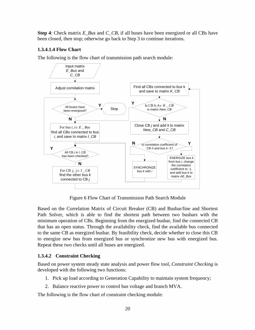
20

Step 4: Check matrix E_Bus and C_CB, if all buses have been energized or all CBs have been closed, then stop; otherwise go back to Step 3 to continue iterations.

1.3.4.1.4 Flow Chart The following is the flow chart of transmission path search module:

Input matrix E_Bus and

C_CB

Adjust correlation matrix

Stop

All CB j in I_CB has been checked?

All buses have been energized?

N

Y

Find all CBs connected to bus k and save to matrix K_CB

N

Is correlation coefficient of CB h and bus k -1?

SYNCHRONIZE bus k with i

Y

N

ENERGIZE bus k from bus i, change

the correlation coefficient to -1, and add bus k to matrix AE_Bus

find all CBs connected to bus i, and save to matrix I_CB

For bus , _i i E Bus∈

find the other bus k connected to CB j

For CB , _j j I CB∈

in matrix New_CBIs CB , _h h K CB∈

Y

Close CB j and add it to matrix New_CB and C_CB

YN

Figure 6 Flow Chart of Transmission Path Search Module

Based on the Correlation Matrix of Circuit Breaker (CB) and Busbar/line and Shortest Path Solver, which is able to find the shortest path between two busbars with the minimum operation of CBs. Beginning from the energized busbar, find the connected CB that has an open status. Through the availability check, find the available bus connected to the same CB as energized busbar. By feasibility check, decide whether to close this CB to energize new bus from energized bus or synchronize new bus with energized bus. Repeat these two checks until all buses are energized.

1.3.4.2 Constraint Checking Based on power system steady state analysis and power flow tool, Constraint Checking is developed with the following two functions:

1. Pick up load according to Generation Capability to maintain system frequency;

2. Balance reactive power to control bus voltage and branch MVA.

The following is the flow chart of constraint checking module:

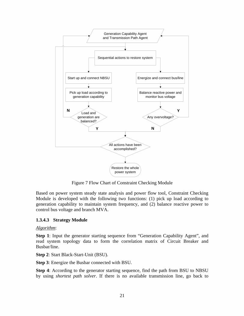
21

Generation Capability Agent and Transmission Path Agent

Sequential actions to restore system

Restore the whole power system

Load and generation are

balanced?

N

Y

Start up and connect NBSU

Pick up load according to generation capability

Energize and connect bus/line

Balance reactive power and monitor bus voltage

Any overvoltage?

N

Y

All actions have been accomplished?

Figure 7 Flow Chart of Constraint Checking Module

Based on power system steady state analysis and power flow tool, Constraint Checking Module is developed with the following two functions: (1) pick up load according to generation capability to maintain system frequency, and (2) balance reactive power to control bus voltage and branch MVA.

1.3.4.3 Strategy Module AlgorithmStep 1: Input the generator starting sequence from “Generation Capability Agent”, and read system topology data to form the correlation matrix of Circuit Breaker and Busbar/line.

:

Step 2: Start Black-Start-Unit (BSU).

Step 3: Energize the Busbar connected with BSU.

Step 4: According to the generator starting sequence, find the path from BSU to NBSU by using shortest path solver. If there is no available transmission line, go back to

22

“Generation Capability Agent” and find new generator starting sequence. Save the sequence to Busbar_Path and CircuitBreaker_Path.

Step 5: Provide cranking power along the path to start Non-Black-Start-Unit (NBSU) and synchronize NBSU with its connected busbar. If any violation reported from “Constraint Checking Agent”, go back to “Generation Capability Agent” and find new sequence, and then go to shortest path solver to get a new path.

Step 6: Build the entire transmission system by “Transmission Path Agent”. If any violation reported from “Constraint Checking Agent”, go back to shortest path solver to get a new path.

Step 7: Distribution Agent to restore distribution system and restore the whole power system.

The following is the flow chart of strategy module:

System data and Generator data

Generation Capability Agent to provide optimal starting sequence

Any violation from Constraint Checking Agent?

Restore the whole power system

Y

Form correlation coefficient matrix of CB and Busbar

Start BSU, energize connected bus and pick up substation load

Shortest Path Solver to provide path from BSU to NBSU

N

Y

Transmission Path Agent to build the transmission system and pick up load

Distribution System AgentN

Provide cranking power to start NBSU, synchronize the connected

bus and pick up load



N

Y

Figure 8 Flow Chart of Strategy Module

The Transmission Path Search Module, Constraint Checking Module and Strategy Module developed in this section are used to illustrate how Generation Capability Optimization module provide solutions and cooperate with other modules. More detailed and advanced models are developed in Part II and Part III in this report.

23

1.4 Numerical Results

In this research, the software tool of ILOG CPLEX is used to solve the proposed MIQCP. CPLEX provides Simplex Optimizer and Barrier Optimizer to solve the problem with continuous variables, and Mixed Integer Optimizer to solve the problem with discrete variables. ILOG CPLEX Mixed Integer Optimizer includes sophisticated mixed integer preprocessing routines, cutting-plane strategies and feasibility heuristics. The default settings of MIP models are used with a general and robust branch & cut algorithm.

1.4.1 Case of Four-generator System A four-generator system with fictitious data is studied to illustrate the “Two-Step” algorithm. Table 1 gives the generator characteristic data.

Table 1 Data of Generator Characteristic

i Tctp Tcmin Tcmax Rr (MW/ per unit time)

Pstart (MW)

Pmax (MW)

1 2 N/A 5 2 1 8 2 1 5 N/A 4 1 12 3 2 N/A 4 4 2 20 4 1 N/A N/A 1 N/A 3

In this system, there are 3 NBS generators and 1 BS generator. Among the 3 NBS generators, 2 units have Tcmax and 1 unit have Tcmin. The total restoration time is set to be 12 time unit. The optimal starting time for all generating units is obtained after 5 iterations by applying proposed method, as shown in Table 2.

Table 2 Generator Starting Time

Unit tstart (per unit time)

1 2 2 5 3 4 4 0

Table 3 gives the generator status for the optimal solution:

24

Table 3 Generator Status for the Optimal Solution

NBS Generator System Generation Capability (MW) i=1 i=2 i=3 i=4

t=0 0 0 0 1 0 t=1 0 0 0 1 0 t=2 1 0 0 1 0 t=4 1 0 1 1 0 t=6 1 1 1 1 3 t=12 1 1 1 1 39

Figure 9 shows the time instants where generators change to the respective second segment of the capability function. The red line is system total generation capability curve.

(MW)genP

t

G1G2

G3

G40

1 2 4 5

Start G4

Start G1Start G3

Start G2

T3

Figure 9 Two Steps of Generation Capability Curve

The following stages summarize how the restoration process progresses:

1. In the beginning, BS generator G4 is started up t=0, and add it to ASG.

2. In time period 1, according to criterion (4), set t=t4start+t4ctp=1, and solve the problem. Update generation capability function of G4 to P4gen2(t).

3. In time period 2, by criterion (1), set t=1+1=2, and solve the problem. It is shown that NBS generator G1 is started, and add it to ASG.

4. Then in time period 3, set t=t1start+t1ctp=4 by criterion (4), and solve the problem again. It is shown NBS generator G3 is started, and add it to ASG. Update generation capability function of G1 to P1gen2(t).

25

5. In time period 4, set t=t3start+t3ctp=6 according to criterion (4) and solve the problem. NBS generator G2 is started, and adds it to ASG. Update generation capability function of G3 to P3gen2(t).

6. In time period 4, according criterion (3), set t=T=12, and solve the problem.

As shown in Fig. 4, there are a total of five time periods to calculate the optimal solution for four-generator system.

1.4.2 Case of PECO System The proposed “Two-Step” algorithm is applied to the generation in the PECO system. For simplicity, units at the same station with similar characteristics are aggregated into one [1]. Table 4 gives the generator characteristic data.

Table 4 Data of Generator Characteristic

Unit Type Tctp (hr)

Tcmin (hr)

Tcmax (hr)

Rr (MW/hr)

Pstart (MW)

Pmax (MW)

Chester_4-6 CT N/A N/A N/A 120 N/A 39 Conowingo_1-11 Hydro N/A N/A N/A 384 N/A 560 Cromby_1-2 Steam 1:40 N/A N/A 148 8 345 Croydon_1 CT 0:30 5:00 N/A 120 6 384 Delaware_9-12 CT N/A N/A N/A 162 N/A 56 Eddystone_1-4 Steam 1:40 3:20 N/A 157 12 1341 Eddystone_10-40 CT N/A N/A N/A 168 N/A 60 Falls_1-3 CT N/A N/A N/A 135 N/A 51 Moser_1 CT N/A N/A N/A 90 N/A 51 Muddy Run_1-8 Hydro 0:30 N/A N/A 246 13.2 1072 Richmond_91_92 CT N/A N/A N/A 288 N/A 96 Schuylkill_1 Steam 2:00 N/A 2:30 135 2.7 166 Schuylkill_10-11 CT N/A N/A N/A 84 N/A 30 Southwark_3-6 CT N/A N/A N/A 156 N/A 52 CCU1 CC 2:40 N/A 3:20 108 5 500 CCU2 CC 2:00 2:30 N/A 162 7.5 500 In this system, there are 7 NBS generators and 9 BS generators. Among 7 NBS generator, there are 2 units have Tcmax and 3 other units have Tcmin. The total restoration time is set to be 15 hrs, which is divided into 90 time slots with the 10 min length of each time slot.

After blackout, the optimal starting time for all generating units is obtained after 9 iterations by applying the proposed algorithm, as shown in Table 5.

26


i Unit tstart (hr) 3 Cromby_1-2 0:10 4 Croydon_1 5:00 6 Eddystone_1-4 3:20 10 Muddy Run_1-8 0:10 12 Schuylkill_1 0:10 15 CCU1 0:10 16 CCU2 2:30

Table 6 gives the generator status for the optimal solution:

Table 6 Generator Status for the Optimal Solution

NBS Generator System

Generation Capability (MW) i=3 i=4 I=6 i=10 i=12 i=15 i=16

t=0 0 0 0 0 0 0 0 0 t=1 1 0 0 1 1 1 0 264.5 t=4 1 0 0 1 1 1 0 623.1 t=11 1 0 0 1 1 1 0 1166.1 t=13 1 0 0 1 1 1 0 1297.4 t=17 1 0 0 1 1 1 1 1642.6 t=27 1 0 1 1 1 1 1 2460.8 t=30 1 1 1 1 1 1 1 2718.8 t=33 1 1 1 1 1 1 1 2926.3 t=90 1 1 1 1 1 1 1 5084.3

Figure 10 shows the time instants where generators change to the respective second segment of the capability function. The red line is system total generation capability curve.

27

(MW)genP

t0 T

G5,7,8,9,14

G6

G11G1,G13

G15,G16

G12G3

G10G2G4

1 2 3 4 6 7 9

Start G1,G2,G5,G7,G8,G9,G11,G13,G14

Start G3,G10,G12,G15

Start G16Start G6

5 8Start G4

Figure 10 Two Steps of Generation Capability Curve

The following is a summary of the restoration process:

1. In the beginning, BS generator G1, G2, G5, G7, G8, G9, G11, G13 and G14 are started at t=0, and add them to ASG.

2. In time period 1, since none of BS generators have characteristic of Tctp, according to criterion (1), set t=0+1=1, and solve the problem. It is shown that NBS generator G3, G10, G12 and G15 are started, and add them to ASG.

3. In time period 2, by criterion (4), set t= t10start+t10ctp=4, and solve the problem. Update generation capability curve of G10 to P10gen2(t).

4. Then in time period 3, set t= t3start+t3ctp=11 by criterion (4), and solve the problem again. Update generation capability curve of G3 to P3gen2(t).

5. In time period 4, set t= t12start+t12ctp=13 according to criterion (4), and solve the problem again. Update generation capability curve of G12 to P12gen2(t).

6. In time period 5, according to criterion (4), set t= t15start+t15ctp=17, and solve the problem again. It is shown that NBS generator G16 is started at t=15, and add it to ASG. Update generation capability curve of G15 to P15gen2(t).

7. In time period 6, by criterion (4), set t= t16start+t16ctp=27, and solve the problem again. It is shown that NBS generator G6 is started at t=20, and add it to ASG. Update generation capability curve of G16 to P16gen2(t).

28

8. In time period 7, set t= t6start+t6ctp=30 by criterion (4), and solve the problem again. It is shown that NBS generator G4 is started at t=30, and add it to ASG. Update generation capability curve of G6 to P6gen2(t).

9. In time period 8, by criterion (4), set t= t4start+t4ctp=33, and solve the problem. Update generation capability curve of G4 to P4gen2(t).

10. In time period 9, according criterion (3), set t=T=90, and solve the problem.

There are a total of nine time periods, as shown in Figure 10, to solve the optimization problem for the PECO-Energy system.

1.4.3 Case of IEEE 39-Bus System The IEEE 39-Bus system is used for illustration of the Generation Capability Optimization Module and the integration of the software modules. Figure 11 shows the system topology.

G1

30

39

1

2

25

3729

17

26

9

3

38

16

5

4

18

27

28

3624

35

22

21

20

34

23

19

33

10

11

13

14

15

8 31

126

32

7

G10 G8

G1

G2 G3 G5 G4 G6

G9

G7

Figure 11 IEEE 39-Bus System Topology

There are 10 generators and 39 buses. It is assumed that the scenario is a total blackout. G10 is a black start unit (BSU) and G1 – G9 were all non black start units (NBSUs). Generator data are shown in Table 7.

29

Table 7 Data of IEEE 39-Bus System

Gen. Tctp (hr)

Tcmin (hr)

Tcmax (hr)

Rr (MW/hr)

Pstart (MW)

Pmax (MW)

G1 0:35 0:40 N/A 215 5.5 572.9 G2 0:35 N/A N/A 246 8 650 G3 0:35 N/A 2:00 236 7 632 G4 0:35 1:10 N/A 198 5 508 G5 0:35 N/A 1:00 244 8 650 G6 0:35 N/A N/A 214 6 560 G7 0:35 N/A N/A 210 6 540 G8 0:35 N/A N/A 346 13.2 830 G9 0:35 N/A N/A 384 15 1000 G10 0:15 N/A N/A 162 0 250

Step 1

By utilizing Generation Capability Optimization Module to get the optimal starting time for all NBS generation units:

:


Gen. 1 2 3 4 5 6 7 8 9 Tstart (hr) 0:50 0:30 0:20 1:10 0:40 0:20 0:30 0:30 0:40

Step 2

The following times to complete GRAs are considered in searching for the transmission path [12]:

:

Table 9 Time to Complete GRAs

Generic Restoration Action (GRA) Time (min.) Restart BSU 15 Energize Busbar from BSU/busbar/line 5 Connect Tie Line 25 Crank a NBSU from a Busbar 15 Synchronize between Busbar/Lines 20 Pick up Load 10

BSU G10 is connected to system at t=0:15 (hr).

Step 2.1: Start BSU

Table 10

Step 2.2: Provide cranking power to start NBSU

and Figure 12 show the transmission path for already started generators to provide cranking power to NBSU.

30

Table 10 Transmission Path

NBS Gen.

Gen. provide cranking power Transmission Path

G1 G10 Bus: 30→2→1→39 G2 G10 Bus: 30→2→3→4→5→6→31 G3 G10 Bus: 30→2→3→4→14→13→10→32 G4 G10 Bus: 30→2→3→18→17→16→19→33 G5 G10 Bus: 30→2→3→18→17→16→19→20→34 G6 G10 Bus: 30→2→3→18→17→16→21→22→25 G7 G10 Bus: 30→2→3→18→17→16→21→22→23→36 G8 G10 Bus: 30→2→25→37 G9 G10 Bus: 30→2→25→26→29→38

G1

30

39

1

2

25

3729

17

26

9

3

38

16

5

4

18

27

28

3624

35

22

21

20

34

23

19

33

10

11

13

14

15

8 31

126

32

7

G10 G8

G1

G2 G3 G5 G4 G6

G9

G7

Figure 12 Optimal Transmission Path

If there is not enough cranking power at the planned starting time, add the corresponding constraint and go back to Generation Capability Optimization Module to calculate the new start-up sequence.

(1) At t=0:20 (hr) G3 and G6 are planned to be started up. However, there is not enough cranking power since it takes some time to energize buses to transfer cranking power. Then, the shortest path for BSU to provide cranking power to start NBSU is from G10 to G8, which need 15 more minutes to energize buses along the transmission path. Therefore, there will not be available cranking power for any NBSU before t=0:35 (hr). Add the following constraint:

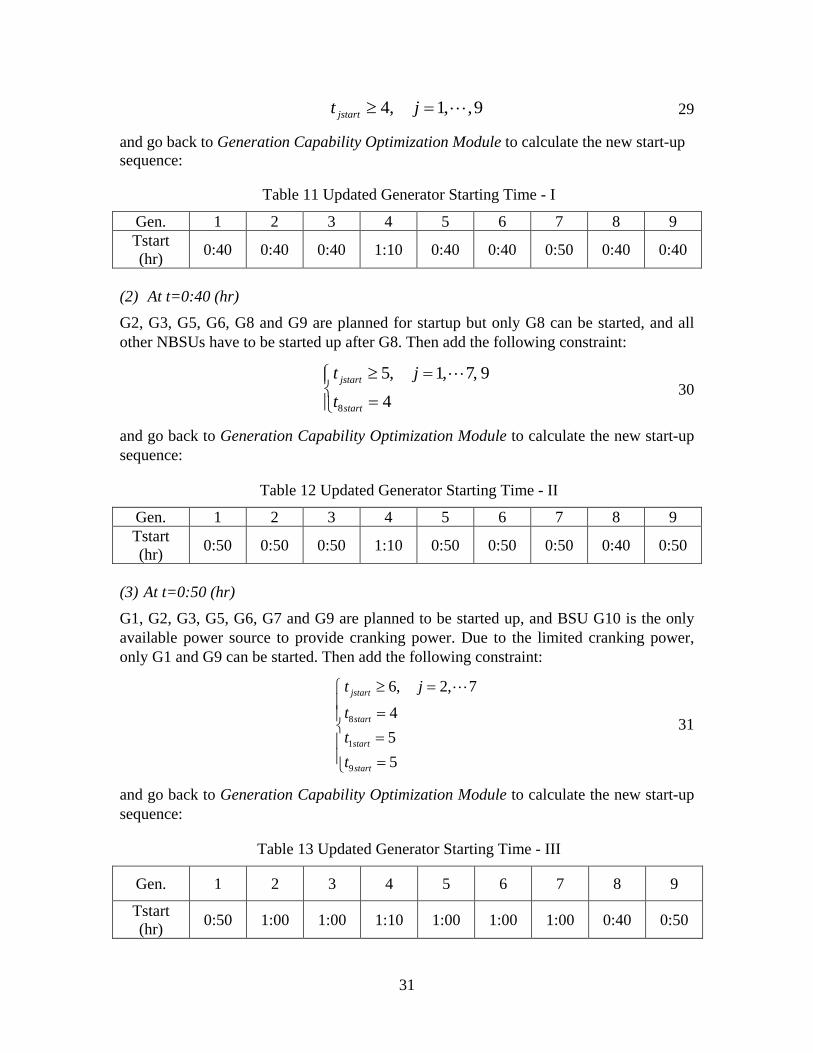
31

4, 1, ,9jstartt j≥ = 29

and go back to Generation Capability Optimization Module to calculate the new start-up sequence:

Table 11 Updated Generator Starting Time - I

Gen. 1 2 3 4 5 6 7 8 9 Tstart (hr) 0:40 0:40 0:40 1:10 0:40 0:40 0:50 0:40 0:40

(2) At t=0:40 (hr) G2, G3, G5, G6, G8 and G9 are planned for startup but only G8 can be started, and all other NBSUs have to be started up after G8. Then add the following constraint:

8

5, 1, 7, 9

4jstart

start

t jt

≥ =

=

30


Table 12 Updated Generator Starting Time - II

Gen. 1 2 3 4 5 6 7 8 9 Tstart (hr) 0:50 0:50 0:50 1:10 0:50 0:50 0:50 0:40 0:50

(3) At t=0:50 (hr) G1, G2, G3, G5, G6, G7 and G9 are planned to be started up, and BSU G10 is the only available power source to provide cranking power. Due to the limited cranking power, only G1 and G9 can be started. Then add the following constraint:

8

1

9

6, 2, 7

455

jstart

start

start

start

t jttt

≥ =

=

= =

31


Table 13 Updated Generator Starting Time - III

Gen. 1 2 3 4 5 6 7 8 9

Tstart (hr) 0:50 1:00 1:00 1:10 1:00 1:00 1:00 0:40 0:50

32

(4) At t=1:00 (hr) G2, G3, G5, G6 and G7 are planned for start up, and BSU G10 is able to provide enough cranking power. They can all be started, and finally, G4 will be started at t=1:10 (hr).

Step 2.3: Build system skeleton by utilizing Transmission Path Search Module. Step 3

Table 14

:

provides the updated actions by Constraint Checking Module:

Table 14 Actions Provided by Constraint Checking Module

Time (hr) Bus Violation Action 0:20 2 Overvoltage Postpone connecting G10 0:25 1,2,3,25 Overvoltage Postpone connecting G10

0:30 N/A N/A Pick up load at Bus 2,4,18, 25,26,29 and connect G10

0:35 26,29 Overvoltage Energize Bus 27 0:40 29,38 Overvoltage Postpone connecting G8 0:45 28,39 Overvoltage Pick up load at bus 28,29 0:50 N/A N/A Energize Bus 38 0:55 N/A N/A Start G9

In the above table, actions at t=0:35 (hr) are provided by applying several modules together. First, Constraint Checking Module provided that Bus 26 and 29 have overvoltage of 1.120 p.u. and Bus 29 cannot be energized. Then go back to Transmission Path Search Module to find a new path. However, the alternative path by energizing Bus 28 and 27 still caused an overvoltage. Therefore, only bus 27 can be energized by calculating with Constraint Checking Module.

By the cooperation of three modules, the whole system was successfully restored.

Table 15 shows all the actions to restore the whole power system to a normal state at each time slot.

33

Table 15 Actions to Restore Whole Power System

Time (hr) Action Target t=0:15 Energize Bus 30 t=0:20 Energize Bus 2 Branch 30-2 t=0:25 Energize Bus 25,1,3 Branch 2-25,2-1,2-3 t=0:30 Energize Bus 37,39,26,4,18 Energize Branch 25-37,1-39,25-26,3-4,3-18 Connect G10 t=0:35 Energize Bus 27,5,14,17 Branch 26-27,4-5,4-14,18-17 t=0:40 Energize Bus 6,13,16 Branch 5-6,14-13,17-16 t=0:45 Energize Bus 10,19,21,24,28,29,31 Branch13-10,16-19,16-21,16-24,26-28,26-29, 6-31 t=0:50 Energize Bus 20,22,23,32,33,38 Branch 19-20,21-22,24-23,10-32,19-33,29-38 Crank G8,G1 t=0:55 Energize Bus 34,35,36 Branch 20-34,22-35,23-36 Crank G9 t=1:00 Crank G2,G3,G5,G6,G7 t=1:10 Crank G4 t=1:25 Connect G1,G8 t=1:30 Connect G9 t=1:35 Connect G2,G3,G5,G6,G7 t=1:45 Energize Bus 9,8,7,11,15,12 Branch 39-9,5-8,6-7,6-11,14-15,13-12,22-23 t=1:40 Connect G4 t=1:50 Energize Branch 29-28,10-11,17-27,16-15,9-8,8-7,11-12

34

Figure 13 shows the comparison of system generation capability curves by using different modules:

0 5 10 15 20 25 30 35 400

1000

2000

3000

4000

5000

6000

time T (pu)

Gen

erat

ion

Cap

abili

ty P

(MW

)Generation Capability Curve

Using Generation CapabilityOptimization ModuleUsing Generation CapabilityOptimization and TransmissionPath Search ModulesUsing Generation CapabilityOptimization, Transmission PathSearch and Constraint Checking Modules

Figure 13 Comparison of Generation Capability Curves by Using Different Modules

Figure 14 shows the restoration progress at each major time slot:

35

30

1

2

25

3

G1

30

39

1

2

25

3726

3

4

18

G10

G1

30

39

1

2

25

37

17

26

3

5

4

18

27

14

G10

t=0:25 t=0:30

t=0:35

G1

30

39

1

2

25

37

17

26

3

16

5

4

18

27

13

14

6

G10

G1

30

39

1

2

25

3729

17

26

3

16

5

4

18

27

28

24

21

19

10

13

14

31

6

G10

G1

30

39

1

2

25

3729

17

26

3

38

16

5

4

18

27

28

24

22

21

20

23

19

33

10

13

14

31

6

32

G10 G8

G1

t=0:40 t=0:45

t=0:50

G1

30

39

1

2

25

3729

17

26

3

38

16

5

4

18

27

28

3624

35

22

21

20

34

23

19

33

10

13

14

31

6

32

G10 G8

G1

G1

30

39

1

2

25

3729

17

26

9

3

38

16

5

4

18

27

28

3624

35

22

21

20

34

23

19

33

10

11

13

14

15

8 31

126

32

7

G10 G8

G1

G2 G3 G5 G4 G6

G9

G7

t=0:55

t=1:45

Figure 14 Progress of Restoring Power System

36

1.4.4 Case of Western Entergy Region After the disturbance in Western Region of the Entergy System in June 2005, two 260 MW generating units at Lewis Creek and the Frontier generator were tripped offline. Western Region was separated from the rest of the Entergy System. It is assumed that these 4 generators were ready to be started and synchronized, and there was black start power from outside to start 1 generator. Table 16 provides four generators’ characteristics:

Table 16 Data of Four Generators

Generator Tctp (hr)

Tcmin (hr)

Tcmax (hr)

Rr (MW/hr)

Pstart (MW)

Pmax (MW)

G1 2:40 N/A 3:00 108 5 260 G2 2:40 N/A 3:00 120 6 260 G3 2:00 N/A 2:30 165 3.3 165 G4 1:40 N/A 3:20 148 8 310

After 1.32 second of computational time, Generation Capability Optimization Module provides the optimal solution as following:


Generator G1 G2 G3 G4 Tstart (hr) 3:00 2:50 3:10 2:40

The characteristic of fast response is able to assist operators during the whole restoration progress. Figure 15 provides the system generation capability curve:

0 10 20 30 40 50 600

100

200

300

400

500

600

700

800

900

1000

time T (pu)

Gen

erat

ion

Out

put (

MW

)

Generation Capability Curve


37

1.4.5 Performance Analysis of MILP Method

Table 18 Performance Analysis

System Four-Gen. PECO IEEE 39-Bus Number of NBS generators 3 6 9 Number of all generators 4 15 10 Total restoration time (hr) 2 5 7

Number of decision variables 429 4998 6327 Number of constraints 1119 13842 17847

Max Generation Capability 167.5 60683 167403 Computational time (sec.) 1.41 8.63 13.71

From the simulation results, it is concluded that the computational time can be kept within the practically feasible time.

1.4.6 Comparison with Other Methods Table 19 gives the computational time by using each of these developed methods to provide initial generator starting time in IEEE 39-Bus system. The MILP method proposed in this paper can provide an accurate and global optimal solution with satisfactory computational performance.

Table 19 Comparison with Other Methods

Algorithm Global Optimality Computational Time 1. Enumeration Yes 1 hour and 53 minutes 2. Dynamic Programming No 55 minutes 3. Two-Step No 4 minutes 4. MIQCP No 35 minutes 5. MILP Yes 8 seconds

38

1.5 Conclusions

In this research, the generator start-up sequencing problem is formulated as a MIQCP optimization problem for determining an optimal generator start-up strategy for power system restoration following a blackout. Incorporating the proposed “Two-Step” algorithm to take advantage of the quasiconcave property of generation capability curve, the optimization problem can be solved with available convexity-based optimization tools. The numerical results demonstrate the effectiveness of the algorithm. While the solution provides system operators an optimal start-up sequence of the generators at the start of the system restoration, system operators need to identify transmission paths and pick up critical loads as the restoration effort continues.

An MILP-based optimal generator start-up strategy for bulk power system restoration following a total blackout is proposed. By applying four techniques to nonlinear generation capability curve, a MILP model of generation capability optimization is formulated and an algorithm incorporating the actual system conditions is proposed. The numerical results demonstrate the effectiveness of the algorithm. Global optimality is obtained and guaranteed by the proposed strategy. Collaborating with transmission path finding, constraint checking and strategy coordination, the proposed model provide system operators with the start-up sequence of the generators.

The contribution of this research is in the formulation of the generator starting sequence problem into a rigorous mathematical programming problem. Compared to the empirical solutions based on heuristic methods or other knowledge-based approaches, true optimal solutions are ascertained. This formulation does not depend on specific software tools or computer languages.

39

Part II. Transmission System Restoration with Constraints

Checking

40

2.1 Introduction

2.1.1 Background Power system restoration following a blackout is one of the critical tasks for system operators in the control center. After the system is subjected to a blackout, and the whole system has more than one black start generator, parallel restoration is an efficient way to speed up the restoration process. It is commonly used by utilities in system restoration plans [2]. A common parallel restoration guideline is:

1. Sectionalizing of power system into subsystems

2. Restoration of each island

3. Synchronization of islands.

Most utility companies and reliability regions rely on an off-line restoration plan and the experience of dispatchers to select and implement scenarios for the black start path [2], [30] and procedures to restore the system. Using a restoration plan, designed based on past experience and off line analysis may not be the most reliable approach to come up with a black start plan as it is difficult to predict changing network configurations and loading levels. To address this need, computer tools have been developed and implemented in [31-32] for the on-line operational environment. Since actual outages are hard to predict in the planning stages, the restoration plan only serves as a guide to the operator. When performing system restoration, operators need near real-time system information in order to make decisions under changing system conditions.

The restoration procedure following a power system outage spans three time periods or is a three step process:

1. Sending cranking power to non-black start generators or to the critical loads from the black start generators, or relying on assistance from outside the system

2. Integration of generation and transmission to recreate a skeleton of the bulk power system

3. Minimization of the unserved load [33]

2.1.2 Overview of the Problem The primary constraint to determine whether the parallel restoration of separate islands or subsystems is feasible is dependent on the availability of black start capacity and its geographic distribution across the system. Once it is determined that parallel restoration is feasible with sufficient black start capability being available, finding a systematic approach to define the boundaries of the subsystems can result in a more efficient and accelerated restoration process. Parallel restoration of subsystems requires that sufficient black start capability be available within each subsystem to energize critical equipment and to send power to other non-black start generators. Each subsystem should also have the ability to match generation and load to maintain frequency within prescribed limits [34]. Furthermore, transmission lines and other transmission components must not be loaded above their capacity limits (e.g., thermal capacity limits and steady state stability

41

limits). When the parallel restoration method is used in a given system, the splitting strategy must satisfy three constraints:

1. Each subsystem must have at least one black start generator. All the generators within a subsystem are divided into groups based on their black start sequence and cranking power capability.

2. In each island, generation and load are balanced approximately.

3. No transmission capacity limits are violated.

During restoration of the bulk transmission network the following constraints should be systematically verified and applied to determine the sequence in which the transmission lines should be energized while satisfying the reliability criteria. These criteria include [35]:

• Real and reactive power balance

• Thermal constraints on transmission lines

• Sustained overvoltages during early restoration

• Switching surges

• Unstable phenomenon of self-excitation

• Maintaining steady-state and transient stability during restoration

This report examines the restoration path selection for blacked-out transmission systems based on efficient checking of the thermal, transient stability and voltage constraints on the transmission system after the affected area has sufficient power supply/generation available. It should be emphasized that the algorithm determines the optimum path selection to restore the area, however, the lines identified for restoration may not be energized simultaneously, and each transmission switching operation should be checked and verified carefully for safety constraints prior to energizing the lines.

2.1.3 Report Organization The report is organized into four sections. Section 2 presents an overview of the OBDD-based system sectionalizing strategy. Section 3 presents the PTDF-based restoration path selection algorithm. Section 4 describes the sectionalizing result to restore IEEE-39 bus system and to recreate the system conditions that existed on June 15, 2005, that led to the storm-related outages in the Western region of the Entergy System. Several illustrative examples of the application of the proposed technique for restoring systems are also presented in Section 4. Conclusions drawn from the application are presented in Section 5.

42

2.2 OBDD-Based System Sectionalizing Strategy

2.2.1 Ordered Binary Decision Diagram Model in Power System To create an OBDD for a power system, every branch in the system can be seen as a Boolean variable, with respect to 0 or 1. The branch with number 0 means this branch is open in the final sectionalizing strategy and number 1 means it is closed in the final sectionalizing strategy. So each root node in the binary decision diagram represents one binary combination of all the branch states, which can be tracked by a bottom-up process. All branches are then included in the binary decision diagram. For the different system constraint, if one binary combination of all the branch states satisfies all the constraints, that root node will connect to node “1”. If any constraint violation happens, that root node will connect to node “0”. Then the binary decision diagram can be constructed with any branch order. For a specific power system, there are more than one OBDD diagrams with respect to different branch orders in the binary decision diagram, but there is only one set of solutions. For example, Figure 16 depicts 2 binary decision diagrams with different branch orders on a 6 buses system [36-38]. The branch being open is shown by the dashed line and the branch being closed is depicted by the solid line. The constraint to decide the root node connection is a simple algorithm that the root node will connect to node “1” if line x1 and x2 are both closed, or line x3 and x4 are both closed, or line x5 and x6 are both closed, which is presented as the logic expression 654321 xxxxxx ⊕⊕ . The

results show that the simplest binary decision diagram possible based on different variable ordering.

Figure 16 OBDD of 654321 xxxxxx ⊕⊕ Respect to Different Ordering

To verify that conditions 1) each subsystem must have at least one black start generator and 2) in each subsystem, generation and load mismatch is less than a certain value are satisfied, a graph-theoretic approach called balanced partition (BP) is used. The BP approach has been proven to be NP-complete. NP ("Non-deterministic Polynomial time")

43

is the set of problems whose solutions can be verified by a deterministic Turing machine in polynomial time. The simplest NP problems could be solved in polynomial time, the so called P problems. The NP-complete problems are the most difficult problems among NP problems in the sense that no polynomial time algorithms have been found to solve them. Problems that are at least as hard as NP-complete problems are classified as NP-hard problems. Figure 17 shows the relationship between P, NP, NP-complete and NP-hard problems.

Figure 17 Relationship between P, NP, NP-complete and NP-hard Problem

OBDD is an algorithm widely used to solve a certain type of NP-complete problem, which can be expressed in the form of a binary decision diagram (BDD). After the BDD is built up, OBDD deletes all the duplicate and redundant nodes in the basic BDD, to efficiently simplify the BDD. An example is shown in Figure 18. The simplification changes the original large scale BDD into a much smaller one, from which conclusions can be easily drawn.

Figure 18 Eliminating Duplicate and Redundant Nodes

The whole binary diagram has NL levels. By reducing irrelevant nodes and edges, the original power network is simplified and facilitates an efficient solution. The steps of this approach are depicted in Figure 19 below.

P NP

NP - c

NP - hard

44

(a) Converge root node “0” and “1”

(b) Delete the duplicate nodes

(c) Delete the redundant nodes

Figure 19 Steps of Reducing Irrelevant Nodes and Edges

45

From the OBDD simplification, it is straight forward to get the solution to the BP problem depicted in Figure 19. There are 3 paths, associated with 7 solutions, and the result is shown in Table 20. In the table, “1” means the branch it represents is closed. “X” means the branch can be closed or open, the OBDD constraint checking result will remain the same.

Table 20 Result of OBDD Simplification

X1 X2 X3 X4 1 1 1 X X 2 0 X 1 1 3 1 0 1 1

2.2.2 Ordering of Branches and NP-Complete Solution Actually the OBDD procedure does not convert the NP-complete problem to a P problem, because the problems of determining how to order the variables in the diagram are still a NP-complete problem. Figure 20 depicts the relationship between OBDD and NP-completeness.

Balanced Partition (NPc)

Variable Ordering (NPc) OBDD Solution (P)

Figure 20 Using OBDD in BP Problem

If there are NL branches in the power system, there are 2NL possible branch state combinations to check the sectionalizing constraints. The BP problem of a large-scale power system is quite complicated because a combinatorial explosion of its strategy space is unavoidable. Moreover, it is necessary to guarantee both correctness and speed in determining the final splitting strategy to speed up restoration. A strategy based on OBDDs) [39], to search for proper sectionalizing strategies for not-too-large power systems is proposed in [38]. The study of splitting strategies for islanding operation of large-scale power systems using OBDD-based methods shows a correct and efficient way to split power systems into islands to avoid system collapse [37]. Since the BP problem is NP-complete with a large number of decision variables corresponding to transmission lines in a power system, it is reasonable to believe that a good representation (or data structure) for the BP problem can effectively improve solution efficiency. OBDD is just one of such good representations, whose powers have been shown by large industry examples [40-41].

46

2.2.3 Operating Condition and Simulation Result An adaptation of the standard IEEE 39-bus is used to demonstrate the performance of the method. We select BuDDy package (v2.0) [42], which supports all standard OBDD operations and especially many highly efficient OBDD vector operations, to program by C++ language on a PC (Core2 6700-2.66G CPU and 2.0GB DDRAM).

Several assumptions are made before we solve the BP problem. There are 10 generator buses in the system, two of them are assumed to be the black start units. They are bus 30 and bus 36, which are shown in the first row of Table 21. To find all the possible solution among 234≈1.718×1010 possible choices, it is assumed that bus 30 will send cranking power to bus {31, 32, 37 and 39}, bus 36 will send cranking power to bus {33, 34, 35 and 38}. The total generation in the system is 6192.9 MW and the total load is 6150.1 MW. The total generation/load mismatch is smaller than 100 MW inside each subsystem.

Table 21 Generator Data

Bus No. PG (MW) Bus No. PG (MW) 30 250.00 36 560.00 31 572.87 33 632.00 32 650.00 34 508.00 37 540.00 35 650.00 39 1000.00 38 830.00

The Buddy package was developed as part of a Ph.D. project on model checking of finite state machines by Rune M. Jensen. The package has evolved from a simple introduction to BDDs to all the standard BDD operations. With the black start constraint and generation/load constraint checking, the total search time on 34 branches system is less than 4.77 seconds. Only two splitting strategies without any constraint violations are found. The results are shown in Table 22 and Figure 21.

Table 22 Sectionalizing Result

Number Cut-set lines between two subsystems

Generation and load mismatch (MW)

1 3-18, 14-15, 25-26 89.4, -46.6 2 3-18, 4-14, 13-14, 25-26 89.4, -46.6

47

(a) Sectionalizing Strategy No.1

(b) Sectionalizing Strategy No.2

Figure 21 Sectionalizing Strategy on IEEE-39 Bus System

48

In this case, the checking module found 2 solutions for the BP problem. In the real case, once it is determined that parallel restoration is feasible in the system, the dispatchers only need to consider the two selected candidate strategies instead of all 234 strategies. This is a very big saving in time. The operator’s final decision will be made with consideration of the current state of system and availability of alternative generators and lines. The two strategies have the same generation and load value, because bus 14 has no generation or load on it.

49

2.3 PTDF-Based Automatic Restoration Path Selection

2.3.1 Introduction This section examines the restoration path selection for the blacked-out transmission systems based on efficient checking of the thermal, transient stability and voltage constraints on the transmission system after the affected area has sufficient power supply/generation available. The algorithm determines the optimum path selection to restore the area, however, the lines identified for restoration may not to be energized simultaneously, and each transmission switching operation should be checked and verified carefully for safety constraints prior to energizing the lines.

In an effort to reduce the time duration and cost related to service interruption, and to check some of these constraints, several analytical tools have been proposed, such as: expert systems [14, 43] and heuristic approaches [44]. These methods integrate knowledge from the operators and computational algorithms such as power flow and transient stability software to optimize the restoration process and to verify that constraints are not violated. In this report, a computational tool is proposed that can be used to provide guidance to the dispatchers in the operational environment so that system restoration can adapt to the changing system conditions.

2.3.2 PTDF-Based Restoration Path Selection To determine the correct sequence for energizing the lines, the concept of PTDF [45, pg. 421] and weighting factors are used. This idea was originally developed in contingency analysis and evaluated for the removal of branches or the loss of generators at specific nodes. In this paper the novelty of the approach is to plan restoration by calculating the PTDFs for candidate lines to be closed. Even though the concept of PTDF is well established, the use of this idea in system restoration is unique and has not been attempted before. In the approach developed, restoration performance indices (RPIs) will be calculated for ranking two types of branch closures.

During the transmission restoration process, all the newly added lines can be divided into two categories:

1. Radial lines – which will create a branch between an existing node and a new node.

2. Loop closure lines – which will complete paths between two existing nodes.

The restoration time period, in which the transmission system is restored, usually takes 3 to 4 hours [45]. In order to speed up system restoration in the absence of system constraint violations, it is assumed that the radial lines will be candidates to be restored first, rather than loop closure lines.

2.3.2.1 Radial Lines Restoration Performance Index If a line is a radial line between buses i and j, the power flow on the radial line can be considered as a complex bus power injection into the existing system [46, pp. 199-203].

50

The PTDF relating the loading in the line from bus i to bus j with respect to the injected complex bus power Sk on bus k, is denoted as ρij,k.

**

*

, ))()(

(*)(

ij

jkbusikbus

kk

jij

ji

kij zZZ

IV

Vz

VV−

=∂

−∂

=ρ

32

The Zbus elements in the equation above are obtained from the bus impedance matrix referenced to the swing bus. Vi is the bus voltage at bus i. zij is the primitive impedance of the line connecting bus i to bus j. If the distribution factors are arranged in a rectangular array, the power transfer distribution factor matrix can be formed as

NBNBNBNLNLNBNLNL

NB

NB

NLNL S

SS

S

SS

∆

∆∆

=

∆

∆∆

.

.

..........

..

..

.

.2

1

*21

22221

11211

2

1

ρρρ

ρρρρρρ

33

where,

NL is the number of lines in current system

NB is the number of buses in current system

pS∆ is the power flow change on line number p

qS∆ is the power injection change on bus number q

After a new radial line with load at the end of the line is restored in the system, the power flow on the lines that have already been restored will change. The capability of different restored transmission lines to sustain this power flow change will also be different. For example, a lightly loaded line will be able to withstand a higher power flow increase than a moderately loaded line when a radial line with load is restored in the system. The change in power flow with each possible line addition can be estimated using the PTDF calculation with respect to the existing system topology.

If all the restored lines are not close to their thermal limit, the existing power flow expressed as a percentage of the thermal limit on each restored line will be used as a weighting factor ω on the change in power flow (obtained from PTDFs) to evaluate each candidate radial line path restoration. A restoration performance index (RPI) is then evaluated for each candidate radial line considered. The RPI is the sum of the products of the weighting factor and power flow change in each existing transmission line. For each candidate radial line, its RPI is the sum of elements in an NL×1 vector. Then, the candidate radial line with the lowest value of its RPI vector element is restored first. This index is referred to as a Type 1 RPI:

pp

NL

pSRPI ω×∆= ∑

=11 34

51

2.3.2.2 Loop Closure Lines Restoration Performance Index If a line with primitive impedance zij is a loop closure between buses i and j, a new intermediate matrix denoted as Ztemp is considered:

+−+−−

=

ijijoldbusjj

oldbusii

oldbus

oldbusj

oldbusi

oldbusj

oldbusi

old

temp

zZZZZrowZrowZcolZcolZ

Z

)(2)()( 35

To get the new bus impedance matrix, Kron reduction is performed:

Tijloopij

oldbus

newbus ZZZ ∆∆−= 36

)( oldbusj

oldbusiij ZcolZcol −=∆ 37

ijijoldbusjj

oldbusii

oldbusloop zZZZZ +−+= )(2)()( 38

To calculate the updated PTDF ijaddnlm

_,ρ relating the loading in the line from bus l to bus m

with respect to the injected complex bus power Sn on bus n, after adding a line from bus i to bus j, substitute the new bus impedance matrix values obtained from 36 into 38. The PTDF is then given by:

)(])()[(

]})()[(])(){[(])()[(

])()[(

,,*

*

,

*

*

*

*

,

*

*_

,

jlmilmloop

jnoldbusin

oldbus

nlm

lm

jmoldbusim

oldbusjl

oldbusil

oldbus

loop

jnoldbusin

oldbus

nlm

lm

mnnewbusln

newbusijadd

nlm

ZZZ

zZZZZ

ZZZ

zZZ

ρρρ

ρ

ρ

−−

−=

−−−−−=

−=

39

Then, the power transfer distribution factor matrix with the addition of the line from bus i to bus j is obtained as:

ijaddNLNB

ijaddNL

ijaddNL

ijaddNB

ijaddijadd

ijaddNB

ijaddijadd

__2

_1

_2

_22

_21

_1

_12

_11

............

...

...

ρρρ

ρρρρρρ

For each possible loop closure line, a specific matrix Δρadd_line is evaluated.

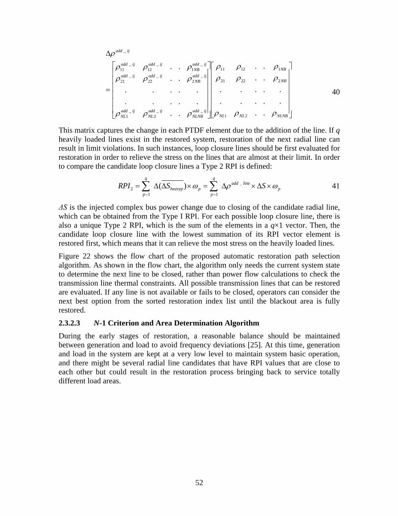
52

=

∆

NLNBNLNL

NB

NB

ijaddNLNB

ijaddNL

ijaddNL

ijaddNB

ijaddijadd

ijaddNB

ijaddijadd

ijadd

ρρρ

ρρρρρρ

ρρρ

ρρρρρρ

ρ

............

..

..

............

..

..

21

22221

11211

__2

_1

_2

_22

_21

_1

_12

_11

_

40

This matrix captures the change in each PTDF element due to the addition of the line. If q heavily loaded lines exist in the restored system, restoration of the next radial line can result in limit violations. In such instances, loop closure lines should be first evaluated for restoration in order to relieve the stress on the lines that are almost at their limit. In order to compare the candidate loop closure lines a Type 2 RPI is defined:

plineadd

q

ppheavyp

q

pSSRPI ωρω ×∆×∆=×∆∆= ∑∑

==

_

112 )( 41

ΔS is the injected complex bus power change due to closing of the candidate radial line, which can be obtained from the Type I RPI. For each possible loop closure line, there is also a unique Type 2 RPI, which is the sum of the elements in a q×1 vector. Then, the candidate loop closure line with the lowest summation of its RPI vector element is restored first, which means that it can relieve the most stress on the heavily loaded lines.

Figure 22 shows the flow chart of the proposed automatic restoration path selection algorithm. As shown in the flow chart, the algorithm only needs the current system state to determine the next line to be closed, rather than power flow calculations to check the transmission line thermal constraints. All possible transmission lines that can be restored are evaluated. If any line is not available or fails to be closed, operators can consider the next best option from the sorted restoration index list until the blackout area is fully restored.

2.3.2.3 N-1 Criterion and Area Determination Algorithm During the early stages of restoration, a reasonable balance should be maintained between generation and load to avoid frequency deviations [25]. At this time, generation and load in the system are kept at a very low level to maintain system basic operation, and there might be several radial line candidates that have RPI values that are close to each other but could result in the restoration process bringing back to service totally different load areas.

53

Obtain system status

Line flow close to limit

Compute the PTDFs

No

Yes

Connect the optimal path

All buses have been connected

Evaluate loop closure paths

Restore rest of the lines

Yes

No

Figure 22 Restoration Path Selection Algorithm Flow Chart

The load areas to be restored should be defined by system operators based on system configuration or load priorities. In the proposed approach if there are more than one load areas, the sequence in which to restore the load areas is determined based on the NERC N-1 criterion [47] and system transient security analysis. The area with the largest transient stability margin and least number of insecure contingencies will be restored first.

N-1 contingency analysis is performed on all candidate load areas to be restored using the software package TSAT (DSATools [48]). The severity of a contingency can be assessed using the transient stability index (TSI). The TSI is calculated as follows [49],

100100100max360max360

<<−×+

−= TSITSI

δ

δ 42

δmax is the maximum angle separation of any two generators in the system at the same time in the post-fault response. TSI > 0 and TSI ≤ 0 correspond to stable and unstable conditions respectively. The area with the largest stability margin and least percent insecure contingencies should be restored first. This ensures that the restored load area would be least susceptible to further degradation due to transient instabilities.

54

2.3.2.4 Line Switching Issues When energizing lightly loaded transmission lines or underground cables, the excessive VArs generated by the undercompensated high voltage lines can increase voltages to unacceptable high levels which are referred to as sustained power frequency overvoltages. If not controlled, these voltages could cause serious reactive power imbalance resulting in generator self-excitation, transformer overexcitation and harmonic distortions.

Basically, sustained overvoltages can be controlled by absorbing the reactive power generated by the lightly loaded transmission lines. This can be done in several ways [33]:

• having sufficient under-excitation capability on the generators

• picking up loads with low power factor

• switching on shunt reactors

• adjusting transformer taps

Due to the fact that adjustments of the control variables are subject to the constraints imposed by plant and system operating conditions, the total effect of these control variables will determine whether the long transmission line can be energized successfully or not.

55

2.4 Simulation Results

2.4.1 June 15, 2005 Storm Case in Entergy System 2.4.1.1 Introduction In June 2005, severe thunderstorms precipitated and forced the interruption of three critical lines in the Western region of the Entergy system. The loss of these lines impacted the ability of the electrical system to serve the Western region load because these lines were tie-lines into the Western region. Within seconds, the generation and other critical lines in the area tripped, and over several minutes the Western region separated from the rest of the system [49]. The system was restored back to normal within four hours after the disturbance. The Western region of the Entergy network is shown in Figure 23. The proposed power transfer distribution factor (PTDF) - based restoration path selection method is applied to the Western region storm scenario and IEEE -39 bus system. Moreover, a novel optimal approach to restore the Western region is discussed in this section.

Figure 23 The Western Region of the Entergy System

In the planning case representing summer peak conditions, the Western region load was approximately 1900 MW. Following the storm event a total of 11 lines were tripped separating the Western region from the rest of the Entergy system [49]. The lines that were tripped are shown in Table 23.

56

Table 23 Lines That Separated the Western Region from the System

No. From To 1 Fork Creek (97695) Sam Rayburn (97704) 2 Cheek (97692) Dayton (97632) 3 China (97714) Sabine (97716) 4 China (97714) Amelia (97689) 5 Hightower (97474) Jacinto (97476) 6 Stowell (97707) Shiloh (97725) 7 Cypress (97690) Poco (97494) 8 Kountze (97700) Doucette (97694) 9 Pee Dee (97512) Rivtrin (97536) 10 Grimes (97514) Huntsville (97484) 11 Grimes (97514) Conroe bulk (97459)

Shortly after the disturbance event, the transmission operation center (TOC) operators started to take manual actions to switch the outaged lines back into service. The first manual action recorded in the events summary relating to the outages and the restoration activities is the restoration of the China (97714) - Amelia (97689) line at 19:04:44, approximately 8 minutes after the initial event. The restoration failed because of sustained phase B to ground fault. The first successfully restored line was Kountze (97700) – Doucett (97694) at 19:22:28, approximately 26 minutes after the initial event. The actual restoration process that was followed by the system operators is detailed in Table 24.

Table 24 System Restoration Time Log

No. Time Index 1 19:22:56.000 2955 KTB To DCT 2 19:24:26.000 5295 STW TO SHILOH 3 19:25:47.893 6970 POCO TO CYP 4 20:06:28.000 16515 JAC TO HIGHTOWER 5 21:01:03.000 16250 CNB TO GRI 6 21:12:25.000 6460 RVT TO PEEDEE 7 21:44:03.000 22820 CHEEK TO DAYTON 8 21:57:54.000 13260 SAB TO CHINA

From the details provided in [49], the Lewis Creek units which are the major generating units in the affected area could not meet the immediate load demand because they sustained minor damage during the event. Therefore, the entire power supply for the affected area had to be obtained from outside the affected area. Given this premise it was imperative that critical tie lines be restored first in order to provide an outside source for black start. The application of the proposed path selection algorithm with constraint checking is detailed below.

57

2.4.1.2 Proposed System Restoration The steps taken by the automatic restoration path selection algorithm is as follows:

Step 1: China (97714) is chosen as the power source bus sending cranking power to the generators inside the affected area. China (97714) Substation is one of the four bulk power sources into the region. China (97714) – Jacinto (97476) and China (97714) – Porter (97567) are the only two 230 kV lines in the Western region. There is a total of 1587 MVA power injection capability into the Western region through these two lines. The transmission line China (97714) - Amelia (97689) experienced a sustained fault during the outage and is one of two 230 kV paths to the China Substation. The other line China (97714) – Sabine (97716) is the first line that the TOC operators tried to restore at 19:04:44 [49].

The first step in the proposed approach is to provide power/voltage to the critical generator buses inside the affected area. The goal in this study is to restore voltage to the Lewis Creek (97451, 97452) generating bus/station, if the station is available and not damaged. The single line diagram is shown in Figure 24.

2

9772

10.

9469

2

9772

10.

9469397

478

0.96

20

39747

80.

9620

49754

10.

9489

49754

10.

9489

59747

61.

0135

48.8

012

.20

10.

0082

.17

59747

61.

0135

9754

31.

0037

7.00

1.30

1

9754

31.

0037

9747

11.

0029

8.70

1.00

1

9747

11.

0029

9746

11.

0037

0.00

40.2

91

9746

11.

0037

99745

21.

0000

40.0

0-2

.86

1

99745

21.

0000

10

9745

11.

0000

40.0

0-6

.92

1

10

9745

11.

0000

454.50

81.57

-0.090.77

-450.95182.37

11

454.50

81.57

-0.090.77

-450.95182.37

148

.80

12.2

0

17.

001.

30

0.00

82.1

7

18.

701.

0010.

0040

.29

140

.00

-2.8

6

140

.00

-6.9

2

20.00-3.46

-20.003.87

22

20.00-3.46

-20.003.87

40.00-2.86

-40.004.47

11

40.00-2.86

-40.004.47

Figure 24 Single Line Diagram Connecting Power Source China and Generator Bus

Lewis Creek through Jacinto

Step 2: The Woodlands area is located in the Southwest portion of the Western region, and it has a high concentration of residential and commercial loads. This area includes Conroe (97459), Alden (97544), Goslin (97468) and some other heavily loaded buses. This area is defined as Area I, and the remaining portion of the Western region as Area II. The transmission lines at the boundary between Area I and Area II are shown in Figure 25 and Table 25.

N-1 contingency analysis is then simulated on both areas using TSAT software as described in Section 2.3.2.3. The results show that if Area I is restored first, 4 out of the 68 possible contingencies are insecure and all secure contingencies have an average TSI value of 89.85. However, if Area II is restored first, 16 out of the possible 184 contingencies are insecure and the average TSI for all secure contingencies is 87.98. Hence, based on the relative severity of the dynamic security assessment it is determined that load Area I should be restored before load Area II. Once this has been ascertained the

58

algorithm progresses systematically to determine the transmission paths to restore in order to supply the load in Area I based on the procedure described above.

Figure 25 Loads Areas Boundary in Western Region

Table 25 Boundary Lines between Area I and Area II

No. From To 1 97475 (Cleveland) 97476 (Jacinto) 2 97461 (Lewis Creek) 97471 3 97461 (Lewis Creek) 97466 4 97461 (Lewis Creek) 97458 (Conair) 5 97461 (Lewis Creek) 97544 (Alden) 6 97567 (Porter) 97463 7 97567 (Porter) 97566 8 97459 (Conroe) 97539

Step 3: The transmission lines and loads in Area I are restored based on the RPI values of all possible transmission lines to be restored. The assumption is that the same amount of load at each end of the new radial lines will be energized. The algorithm will choose the line that is closer to the generator buses or power source buses. The system topology is quite similar to that of a tree. When one or more transmission lines are close to their transmission limit, the algorithm will force the tree to create some loops to relieve the

Area I

Area II

59

stress on the branches. This happens to be the line shown below.

• 97461(Lewis Creek)- 97466- 97520 (Fort pipe)

• 97520 (Fort pipe)- 97460- 97456- 97542- 97475 (Cleveland)

• 97476 (Jacinto)-97475 (Cleveland)- 97542

In this step, both types of RPI value calculation are utilized to perform thermal constraint checking. The calculation illustration will be shown in the following section. The system one line diagram after these lines are restored is shown in Figure 26.

19771

41.

0000

11087.36250.73

19771

41.

0000

2

97721 0.9469

2

97721 0.9469

39747

80.

9620

39747

80.

9620

49754

10.

9489

49754

10.

9489

59747

61.

0135

148

.80

12.2

00.

0082

.17

59747

61.

0135

69754

31.

0037

17.

001.

30

69754

31.

0037

79747

11.

0029

18.

701.

00

79747

11.

0029

89746

11.

0037

10.

0040

.29

89746

11.

0037

99745

21.

0000

140

.00

-2.8

6

99745

21.

0000

10

9745

11.

0000

140

.00

-6.9

2

10

9745

11.

0000

11

9746

61.

0002

10.

000.

00

11

9746

61.

0002

12

9745

80.

9987

186

.20

22.0

0

12

9745

80.

9987

13

9752

01.

0024

17.

006.

30

13

9752

01.

0024

14

9746

01.

0026

128

.50

5.60

14

9746

01.

0026

15

9745

61.

0062

114

.50

2.80

15

9745

61.

0062

16

9754

21.

0141

16.

200.

80

16

9754

21.

0141

11087.36250.73

1

454.50

81.57

-0.090.77

-450.95182.37

1

454.50

81.57

-0.090.77

-450.95182.37

148

.80

12.2

0

17.

001.

30

0.00

82.1

7

18.

701.

0010.

0040

.29

140

.00

-2.8

6

140

.00

-6.9

2

2

20.00-3.46

-20.003.87

2

20.00-3.46

-20.003.87

1

40.00-2.86

-40.004.47

1

40.00-2.86

-40.004.47

10.

000.

00

186

.20

22.0

0

17.

006.

30

128

.50

5.60

114

.50

2.80

16.

200.

80

9747

5

1.02

041.

0204

9747

5

Figure 26 Single Line Diagram before Connecting the Loop Closure Line Security

(97456) – Jayhawk (97542)

Then, the remaining lines in Area I are then restored. These include

• 97459 (Conroe)- 97465- 97511- 97566

• 97468 (Goslin)- 97455- 97463

The single line diagram with these lines restored is shown in Figure 27.

60

19771

4

1.0000

19771

4

1.00002

9772

1

0.9469

2

9772

1

0.946939747

8

0.9620

39747

8

0.9620

49754

1

0.9489

49754

1

0.9489

59747

6

1.0135

59747

6

1.0135

69754

3

1.0037

69754

3

1.0037

79747

1

1.0029

79747

1

1.0029

897

461

1.0037

897

461

1.0037

99745

2

1.0000

99745

2

1.0000

10

9745

1

1.0000

10

9745

1

1.0000

119746

61.0002

119746

61.0002

12

9745

8

0.9987

12

9745

8

0.9987

139752

0

1.0024

139752

0

1.0024

149746

0

1.0026

149746

0

1.0026

15

9745

6

1.0062

15

9745

6

1.0062

16

9754

2

1.0141

16

9754

2

1.0141

18

9747

5

1.0204

18

9747

5

1.0204

19

9746

2

0.9999

19

9746

2

0.9999

20

9745

9

1.0011

20

9745

9

1.0011

2197

468

0.9937

2197

468

0.9937

22

9754

4

0.9951

22

9754

4

0.995197

455

9745

525

9746

5

0.9952

25

9746

5

0.9952

9746397463

Figure 27 Single Line Diagram with All Lines Restored in Area I

Step 4: After the transmission lines supplying the load area are fully restored, N-1 contingency analysis is simulated on restored buses as described in Section 2.3.2.3. The maximum load level that can be supplied in order to guarantee that all N-1 contingencies will be secure is determined.

According to the RPI calculation, transmission lines in Area II can be picked up in sequence. After picking up the following lines, the single line diagram is shown in Figure 28 and Figure 29.

• 97566 -97467 (Porter) -97567

• 97467 (Porter) -97533 -97532 (Hickory) -97627 -97754

• 97627 -97723 -97726

• 97723 -97632 (Dayton)

• 97693 (138 kV, China) -97593 -97626 (Raywood) -97724 -97632 (Dayton)

• 97626(Raywood) -97750 -97725(Shiloh)

• 97750 -97748 -97749

• 97461(Lewis) -97483 -97536 (Rivtrin)

• 97461(Lewis) -97545 -97538 -97488 -97519 -97484(Huntsvl)

• 97461 (Lewis) -97464 -97457 -97453

61

• 97459 (Conroe) -97539 -97470 -97469 -97454 -97514

• 97476 (Jacinto) -97479 -97495 -97489 -97494(Poco)

• 97536 (Rivtrin) -97537 -97529 -97499 -97497 -97496 -97518 -97685 -97694(Doucett)

• 97484 (Huntsvl) -97480 -97486 -97485 -97536 (Rivtrin)

• 97484(Huntsvl) -97480 -97487 -97514 (Grimes)

• 97536 (Rivtrin) -97528 -97535 -97552 -97492 -97553 -97494

19771

4

1.0000

19771

4

1.00002

9772

1

0.9469

2

9772

1

0.946939747

8

0.9620397

478

0.9620

49754

1

0.9489

49754

1

0.9489

59747

6

1.0135

59747

6

1.0135

69754

3

1.0037

69754

3

1.0037

79747

1

1.0029

79747

1

1.0029

897

461

1.0037

897

461

1.0037

99745

2

1.0000

99745

2

1.0000

10

9745

1

1.0000

10

9745

1

1.0000

119746

6

1.0002

119746

6

1.0002

12

9745

8

0.9987

12

9745

8

0.9987

139752

0

1.0024

139752

0

1.0024

149746

0

1.0026

149746

0

1.0026

15

9745

6

1.0062

15

9745

6

1.0062

16

9754

2

1.0141

16

9754

2

1.0141

18

9747

5

1.0204

18

9747

5

1.0204

19

9746

2

0.9999

19

9746

2

0.9999

20

9745

9

1.0011

20

9745

9

1.0011

2197

468

0.9937

2197

468

0.9937

22

9754

4

0.9951

22

9754

4

0.9951

23

9745

5

0.9889

23

9745

5

0.9889

24

9746

3

0.9847

24

9746

3

0.9847

25

9746

5

0.9952

25

9746

5

0.9952

26

9755

1

0.9909

26

9755

1

0.9909

27

9756

6

0.9836

27

9756

6

0.9836

28

9746

7

0.9833

28

9746

7

0.9833

29

9753

3

0.9943

29

9753

3

0.9943

30

9753

2

0.9922

30

9753

2

0.9922

31

9772

3

0.9907

31

9772

3

0.9907

32

9762

7

0.9906

32

9762

7

0.9906

33

9775

4

0.9889

33

9775

4

0.9889

34

9756

7

0.9009

34

9756

7

0.9009

35

9769

3

1.0328

35

9769

3

1.0328

36

9759

3

1.0449

36

9759

3

1.0449

37

9762

61.0566

37

9762

61.0566

38

9772

4

1.0659

38

9772

4

1.0659

39

9763

2

1.0732

39

9763

2

1.0732

40

9754

5

1.0037

40

9754

5

1.0037

41

9748

3

1.0365

41

9748

3

1.0365

42

9753

6

1.0622

42

9753

6

1.0622

43

9748

5

1.0623

43

9748

5

1.0623

44

9752

8

1.0621

44

9752

8

1.0621

45

9753

7

1.0597

45

9753

7

1.0597

Figure 28 Single Line Diagram with Partial Area II Restored

62

Figure 29 Single Line Diagram after the Whole Area Is Restored

The resulting load pick up curve obtained by the proposed method is then compared to the actual load pick up curve that was obtained when the Western system was restored by system operators following the storm-related outages. The plot is shown in Figure 30.

From the plot it is observed that the new restoration path strategy generated by the program provides a more efficient approach to restore the unserved load in the system than the actual restoration operation. In addition, the transmission thermal limit and transient stability constraints are also satisfied. It is to be noted that in reality, there may be practical limitations in energizing some of the lines due to damages. Such factors were not considered in the analysis but can be easily implemented by taking the specific lines out of the list of candidate lines for potential energization.

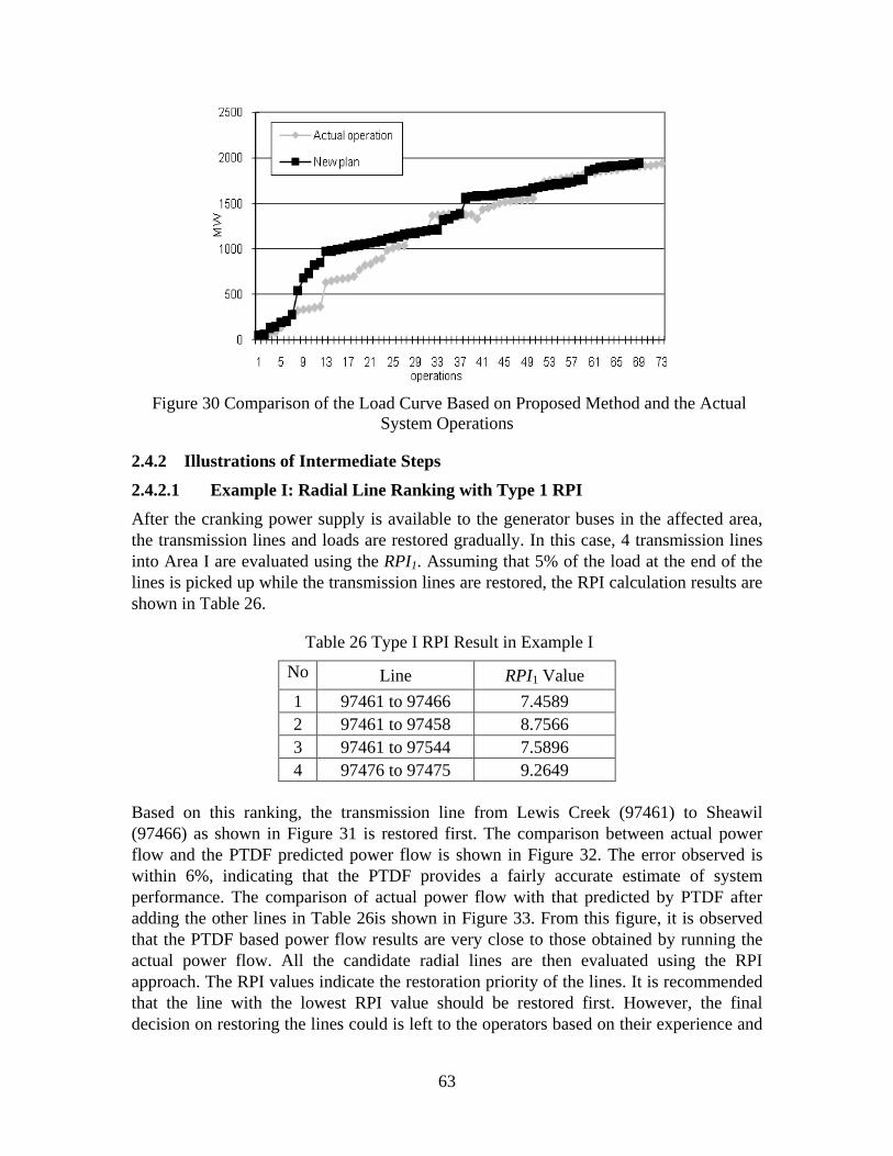
63

Figure 30 Comparison of the Load Curve Based on Proposed Method and the Actual

System Operations

2.4.2 Illustrations of Intermediate Steps 2.4.2.1 Example I: Radial Line Ranking with Type 1 RPI After the cranking power supply is available to the generator buses in the affected area, the transmission lines and loads are restored gradually. In this case, 4 transmission lines into Area I are evaluated using the RPI1. Assuming that 5% of the load at the end of the lines is picked up while the transmission lines are restored, the RPI calculation results are shown in Table 26.

Table 26 Type I RPI Result in Example I

No

Line RPI1 Value 1 97461 to 97466 7.4589 2 97461 to 97458 8.7566 3 97461 to 97544 7.5896 4 97476 to 97475 9.2649

Based on this ranking, the transmission line from Lewis Creek (97461) to Sheawil (97466) as shown in Figure 31 is restored first. The comparison between actual power flow and the PTDF predicted power flow is shown in Figure 32. The error observed is within 6%, indicating that the PTDF provides a fairly accurate estimate of system performance. The comparison of actual power flow with that predicted by PTDF after adding the other lines in Table 26is shown in Figure 33. From this figure, it is observed that the PTDF based power flow results are very close to those obtained by running the actual power flow. All the candidate radial lines are then evaluated using the RPI approach. The RPI values indicate the restoration priority of the lines. It is recommended that the line with the lowest RPI value should be restored first. However, the final decision on restoring the lines could is left to the operators based on their experience and

64

safety considerations.

Figure 31 Single Line Diagram Showing the Radial Line Candidates and the Optimal

Line in RPI Table after Generator Buses are Energized, Example I

Figure 32 Comparison of the Actual Power Flow and PTDF Predicted Power Flow

Figure 33 Comparison of the Actual Power Flow after Adding Lines in Table 26

65

2.4.2.2 Example II: Loop Closure Line Ranking with Type II RPI Since the power flow analysis indicates that the line 97476 – 97543 is within its rated limit, the algorithm developed to determine the sequence in which transmission lines are restored is then applied to determine the next transmission line to be restored. PTDFs and RPI2 are utilized to choose the next line to be energized. Figure 34 shows that when line Lewis Creek (97461) – Sheawil (97466) is close to its thermal limit, the algorithm chooses line Security (97456) – Jayhawk (97542) which connects two buses that have already been energized to be restored next,. The power flow change after closing this line is shown in Table 27 and Figure 35.

Figure 34 Single Line Diagram Showing the Loop Closure Line Security (97456) –

Jayhawk (97542) is Energized due to Line Thermal Limit on Another Line, Example II

Table 27 Type II RPI Result in Example II

No. Line Power Flow Before Closing New Line (MW)

Power Flow After Closing New Line (MW)

1 97456-97542 140.8 102.4 2 97543-97471 132.1 93.6 3 97475-97476 72.9 108.3

66

Figure 35 Comparison of the Power Flow before and after Adding Loop Closure Line

These results reveal that the power flow on the heavily loaded line 97456-97542 reduces from 140.8 MW to 102.4 MW (thermal limit of this line is 206 MVA), and some of the power flow is picked up by the line 97475-97476 (thermal limit of this line is 287 MVA). This relieves the stress on the heavily loaded line and fully utilizes all restored lines to speed up the system restoration.

2.4.2.3 Example III: Sustained Overvoltage Checking and Control Before energizing the transmission lines selected using the RPI approach, sustained overvoltages should be evaluated to make sure no voltage violations occur. A generator terminal voltage violation example in the process of restoring line 97458-97461 is depicted in Figure 36. The generator terminal voltages are shown in Figure 37. Buses 97451 and 97452 are the generator buses inside the area being restored, bus 97714 is the outside black start source, which has a large generation capability.

Figure 36 Single Line Diagram Showing the Transmission Line 97461 – 97458 (the

Dashed Line) to be Energized

67

Figure 37 Generator Terminal Voltage after Restoring the Line 97458-97461

If the generator terminal voltages are reduced to 0.95 p.u. before closing the line, or a shunt reactive source is connected, the generator voltages are within the acceptable limits as shown in Figure 38and Figure 39.

The results show that the sustained overvoltages can be efficiently controlled by methods described in Section 2.2.3.2.4. It is important to note that the extent of the generator's voltage reduction is usually constrained by underexcitation of generators brought about by a number of limiting factors, including generator terminal low voltage limit, reactive ampere limit relay and minimum excitation limit relay. It may be necessary that more than one voltage control method needs to be applied in a given system.

Figure 38 Generator Terminal Voltages are Reduced to 0.95 p.u. before Closing the Line

Generator terminal voltage (pu)

0.00 1.00 2.00 3.00 4.00 5.00 0.95

0.96

0.98

0.99

1.01

1.02

Bus Name 97451 97452 97714

Time (sec)


Time (sec) 0.00 1.00 2.00 3.00 4.00 5.00 0.99

1.01

1.03

1.04

1.06

1.0

Bus Name 97451 97452 97714

68

Figure 39 Generator Terminal Voltages with Shunt Reactive Source Connected

2.4.2.4 Example IV: Load Level Determination after Area I is Fully Restored After the restoration of Area I is complete, the security of the restored transmission lines in Area I have to be maintained before restoring Area II. If the system is vulnerable to line tripping during the restoration process, this security check should be done more frequently. After restoring Area I based on the dynamic analysis, several possible solutions to satisfy N-1 reliability criterion are satisfied by reducing the load level on certain buses as shown in Table 28. The first column in parenthesis shows the MW value of the load, and the percentage value represents the load after reduction as a percentage of the load prior to the outage.

Table 28 Solutions in Example IV

No. Bus Load Level 1 97468(106.24 MW, 40%) 2 97468(185.92 MW, 70%), 97455(102.3 MW, 60%) 3 97468(185.92 MW, 70%), 97463 (60.4 MW, 50%)

4 97468(185.92 MW, 70%), 97544 (70 MW, 50.3%) This analysis determines the upper bound of the load level on these buses during the restoration process of Area I. If the actual system has a particular load requirement, operators can consider the option of reducing other loads.

2.4.3 IEEE-39 Bus System Case In IEEE-39 bus system, which is shown in Figure 40, bus 30 is assumed to be the only black start generator in the system. Two load areas are defined in Table 29. It should be emphasized that the system can be split into more than 2 areas if the system scale is huge.


Time (sec) 0.00 1.00 2.00 3.00 4.00 5.00 0.99

1.00

1.00

1.01

1.01

1.02

Bus Name 97451 97452 97714

69

But the stability constraint checking algorithm will remain the same as described in Section 2.2.3.2.3.

Figure 40 IEEE-39 Bus System

Table 29 Load Areas in IEEE-39 Bus System

Area Bus Number 1 1,3,4,5,6,7,8,9,10,11,12,13,14,17,18,27,31,32,39 2 15,16,19,20,21,22,23,24,25,26,27,28,29,33,34,35,36,37,38

According to the N-1 contingency checking result, which is shown in Table 30, and area determination algorithm, load Area I should be restored first. The whole system will be cranked up by PTDF-based automatic restoration path selection algorithm.

70

Table 30 N-1 Contingency Checking Result

Area Insecure N-1 contingencies

1 0

2 4 It should be noticed that there are totally 12 buses without any generation or load on them. Based on Type I RPI algorithm, this kind of buses will have higher priority compared with generator/load bus. If both of the generator bus and this kind of “empty bus” are ready to be energized, the generator bus will have the priority. The system restoration sequence and the RPI algorithm utilized are shown in Table 31.

Table 31 IEEE-39 Bus System Restoration Path Steps 1 2 3 4 5 6 7 8 9 10

Lines 2-30 1-2 1-39 9-39 8-9 5-8 5-6 6-31 6-7 7-8

Actions RPI1 RPI1 Cranking RPI1 RPI1 RPI1 RPI1 Cranking RPI1 RPI2

Steps 11 12 13 14 15 16 17 18 19 20

Lines 6-31 6-11 10-11 10-32 10-13 13-14 4-5 3-4 12-13 3-18

Actions Cranking RPI1 RPI1 Cranking RPI1 RPI1 RPI1 RPI1 RPI1 RPI1

Steps 21 22 23 24 25 26 27 28 29 30

Lines 17-18 17-27 11-12 2-3 2-25 25-37 25-26 26-28 28-29 29-38

Actions RPI1 RPI1 RPI2 RPI2 Area2 Cranking RPI1 RPI1 RPI1 Cranking

Steps 31 32 33 34 35 36 37 38 39 40

Lines 14-15 15-16 16-19 19-33 19-20 20-34 16-21 21-22 22-35 22-23

Actions RPI1 RPI1 RPI1 Cranking RPI1 Cranking RPI1 RPI1 Cranking RPI1

Steps 41 42 43 44 45 46

Lines 16-24 23-24 16-12 4-14 26-29 26-27

Actions RPI1 RPI2 RPI2 RPI2 RPI2 RPI2

71

2.5 Conclusions

This report provides a method using OBDD to split the system into suitable islands or subsystems that would facilitate restoration. The proposed strategy decomposes the spitting process into two parts: 1) determination of branches order in OBDD, 2) finding the boundary of the islands under the constraints of minimizing the generation-load imbalance.

A systematic method is presented for developing an automatic restoration path selection procedure after a blackout/island occurs. The suggested approach uses the power transfer distribution factor algorithm and weighting factors to determine the optimal restoration sequence for the transmission system. This path selection procedure is performed by checking system thermal constraints, transient stability constraints and voltage constraints. The restoration path selection algorithm is intended to assist the system operator during restoration, by providing a restoration index. Two kinds of restoration performance indices (RPI) are shown. The restoration indices are effective during the restoration of the transmission system as they provide guidance to the operators on how transmission lines should be restored. The algorithm was tested on the Western Region of the Entergy system. The restoration sequence for the transmission lines ensures that the thermal constraint is satisfied during the restoration and can adapt to the changing system conditions. The transient stability constraint is also checked before and after each load area is restored to make sure that the system is secure and stable.

72

Part III. Automated Restoration of Power Distribution Systems

73

3.1 An Introduction to Power System Restoration

3.1.1 The Restoration Process System restoration following a blackout is one of the most important tasks of the dispatchers in the control center. However, few computer tools have been developed and implemented for the on-line operational environment. Indeed, most power systems rely on off-line restoration plans that are developed for selected scenarios of contingencies, equipment outages, and the available resources. Since the actual scenario is hard to predict in the planning stage, the restoration plan can only serve as a guide. Dispatchers need to be aware of the situation and adapt to the changing system conditions during system restoration. In this report, we develop a computational tool that can be used to provide guidance to the dispatchers in the operational environment so that system restoration can adapt to the changing system conditions.

3.1.2 This PSERC Project This project of the Power Systems Engineering Research Center (PSERC) relates to restoration of generation, transmission, and distribution systems. The generation and transmission systems portions are discussed in detail in a separate volume of this report. The main thrust of this report is distribution restoration – as an operator permissive approach to the restoration of the distribution system after a total blackout.

Note that reference [28, 50] resulted from this research work.

3.1.3 An Introduction to Power System Restoration An essential task in the operation of power systems is restoration after a blackout. The restoration process returns the system back to normal operation after any combination of system components have been lost as a result of an outage. In general, restoration is a decision making process in which the system operator executes a set of actions that progressively mitigate the outage. These actions aim at minimizing the impact of the outage on the final user without compromising the security and operability of the system.

Traditionally, guidelines have been developed by utilities to aid the operator in this decision making process [2]. In addition, a common approach used to simplify the restoration task is to divide the restoration process into stages. Fink, Liou and Liu in [3] suggest three stages based on the current operator objective. These are termed: preparation, system restoration and load restoration. The preparation stage evaluates the system configuration after the perturbation and suggests a restoration strategy for the power system, mainly generation and transmission. System restoration focuses on rebuilding the transmission grid, stabilizing the system frequency and the voltage profile, and enhancing the system security. Load restoration follows the other two stages and takes place after some load, generation and transmission have been restored. The governing objective of this stage is to minimize the impact of the outage by gradually reenergizing the distribution system, most notably the system loads.

Due to the nature of the system, there may be some overlap between these stages as the restoration process is performed. Figure 41 Restoration Process Stages illustrates this

73

concept. Dashed ovals represent the stages suggested in [3] while the rectangle shows the end of the restoration process. The solid line circles show the different elements of the power system that must be restored to reach a normal operating state. The overlapping of these circles results from the need of generation, transmission and load to restore each element successfully. The overlapping of the dashed ovals shows how the operator goal changes as the system is restored. In addition, the dashed ovals also show the importance of each of the system elements in each restoration stage. The system perturbation that originates the restorative state plays an important role in defining the extent of the transition and the duration of each stage.

Figure 41 Restoration Process Stages

In spite of the suggested guidelines and stages, restoration remains a very challenging problem for the operator mainly due to the very large number of decision variables present in a power system. In addition, many of these variables are linked to nonlinear models or may have complex interactions with other system elements. This makes the restoration problem very difficult to solve, as it requires very detailed modeling and extensive knowledge of the system to perform this task ‘efficiently’. In fact, the measure of restoration ‘efficiency’ is controversial since it may include any combination of restoration speed, load interrupted, impact on customers, among other factors.

Developing beforehand a set of standard plans that may be used to efficiently restore the system is also complex. Standard plans may not be capable of emulating adequately all the system conditions and in many cases lead to sub-optimal restoration plans. This results from the multiple configurations and different operating conditions that can be attained by a system. In addition, the status or availability of many of the system components after a perturbation may not be readily available to the operator.

In an effort to enhance the restoration process in power systems, a lot of attention has been placed on computational tools and other forms of system automation. Many of these tools seek to reduce the amount of information that operators are exposed to during a restoration process. In some cases these tools interact with the operator and present a set

74

of options that may improve the restoration process, and thus assisting the restoration process. In other cases, automation may be used to execute particular actions that will improve the system based on predefined criteria.

Load restoration, also known as distribution system restoration, has garnered a high level of interest recently. Part of this interest can be attributed to recent practices in power systems related to marketing, deregulation and also technological advances in related fields. The main concern of distribution system restoration becomes the minimization of the outage impact by finding the optimal set (and sequence) of feeders that need to be restored. This may be viewed in a way similar to the unit commitment problem that finds the optimal set of generators that minimize production cost [50]. In fact, the similarities in structure and nature may suggest both problems are duals of each other.

The distribution restoration problem presents several challenges:

• Large system dimension

• Multiple operational objectives

• Desired near simultaneous restoration

• Potential of suboptimal solutions

• Combinatorial nature of the problem.

Some of these challenges have been addressed through proposed analytical tools and several forms of automation. Examples of these include novel approaches that develop restoration plans such as: expert systems [33] and [51], genetic algorithm [52], Monte Carlo approach [53] and heuristics [9] and [10]; and more conventional approaches based on: dynamic programming [25], restoration index [26], interior point technology [54], ranking based methods [55] and a mixed-integer programming technique [56].

3.1.4 Objectives The main objective of this thesis is to enhance the restoration of distribution systems by means of optimization algorithms, in particular, the Lagrangian relaxation method for combinatorial optimization problems. This study seeks to show the applicability characteristics of this analytical tool to the distribution restoration problem. In addition, evaluation of the algorithm performance and total effect of this technique on the distribution system restoration process are particular areas of interest.

Additional specific objectives are:

• To analyze and solve the optimal restoration problem via the Lagrangian relaxation method.

• To develop an appropriate formulation and adequate models for the distribution system restoration problem.

• To test different optimal restoration problem formulations that may result in an improved optimization process in terms of type of solution, algorithm performance and computational requirements.

75

• To compare and contrast the results obtained by the Lagrangian relaxation based subgradient approach with other optimization algorithms used in the industry, if possible.

• To present recommendations regarding the implementation of the algorithm in the distribution restoration problem.

• To test the Lagrangian algorithm potential to obtain optimal solutions, and when possible, estimate the duality gap.

• To use further innovative mathematical tools to solve the distribution system restoration problem.

3.1.5 Literature Review The following section provides a review on some of the literature available on power systems restoration. The subjects reviewed in this section include common issues present in the restoration of the power system and the distribution system restoration problem.

3.1.5.1 Bulk Power System Restoration IssuesBulk power system restoration following a partial or total outage has been a cause of concern since the beginning of power systems. Over the years, restoration has been performed aided by a set of guides and common practices developed by utilities. One of the first efforts to document the different operating practices and procedures related to bulk power system restoration was headed by Adibi in the power system restoration task force report [2]. A second task force report [57] soon followed describing common problems in network restoration and alternatives ways of enhancing the restoration process. In general, most of the problems in restoration can be classified into several fields. These are: reactive power balance, load and generation balance and coordination, monitoring, control, protective systems, energy storage, planning and training [57].

Restoration plans are designed based on the characteristics of the system. Strategies differ depending on the system generation mix (hydro, steam, combined cycles and gas turbines), and also the level of interconnection of the transmission network. In addition the common issues that arise during restoration as well as the initial conditions of the system need to be considered when designing a viable restoration plan.

A critical parameter during restoration is system electrical frequency. Frequency is an indicator of the balance between the power injected to the grid by the generators and the load being served. If the load and the generation are perfectly balanced then the frequency of the system should be the nominal frequency. If there is more load than generation connected to the grid, frequency decreases from the nominal value. In the same context, more generation than load results in a system frequency increase.

Adequate operation is obtained by controlling the electrical frequency near the nominal value and limiting it to a specified range. However, due to the nature of the restoration process, a perfect balance between load and generation at all times may not be possible. In addition, the amount of load that can be picked up at any point during restoration is limited. This is a result of many factors including the turbine-governor characteristics of power plants, and the present system configuration. Accounting for the dynamics of the

76

mechanical and electrical systems is a tedious computation to be performed in a restorative system. Several rules of thumb have been developed from experience to simplify this computation. Operating practices have shown that a single load increment of 5 percent of the synchronized generation results in a frequency decay of not more than 0.5 Hz from its previous value [2]. An approximate method that evaluates the frequency response rate of power plants for maximum load pickup is discussed in [44]. However, these approximations may not be adequate for all systems and more strict rules may be needed to produce a viable restoration plan.

Another important electrical consideration during restoration is voltage profile. In order to obtain satisfactory system operation, voltages must be kept within certain values. Adequate voltage profile is generally achieved by having sufficient reactive power sources capable of fulfilling the system needs. Reactive power is generally supplied and/or controlled by generators, shunt capacitors, synchronous condensers, among others. However, satisfying the reactive power balance condition is not trivial due to its nonlinear behavior and the difficulty this has to travel long distances. In addition, energization of transmission lines results in a sudden change in the reactive power due to the charging phenomena observed in them. These sudden changes, also known as switching transient voltages, generally increase the voltage magnitude to dangerous values depending on the characteristics of the transmission line. These and other issues show the need for adequate allocation of the reactive power sources and also the control capability needed to implement a good restoration plan. Problems in transmission line energization are discussed in [58].

Another critical issue within restoration is load pickup. After experiencing a failure and being out-of-service for some time, many of the loads experience a transient state when reenergized. This transient is commonly known as cold load pickup (CLPU) and is a result of the loss of diversity in loads and also other phenomena such as inrush current. Cold load pickup is dependent on many factors such as length of the outage and weather [59]. On residential feeders, a typical behavior for the cold load pickup is that of an exponentially decaying function similar to the one shown in Figure 42 [60].

Figure 42 Example of Cold Load Pick-up Transient as a Function of Time (From [60])

77

Cold load pickup may present several problems to system operators. As an example, forecasting is very difficult due to the generally unknown composition of loads at the moment of service restoration. General considerations for load modeling during restoration are shown by Adibi in [59]. In addition, this paper suggests a classification for loads. This classification is as follows: thermostatically-controlled loads, manually-restarted loads and fixed loads. Several efforts have been made to understand the cold load pickup phenomenon in restoration systems. A physically based cold load pickup model was developed by Ihara and Schweppe in [61]. McDonald, Bruning, and Mahieu also provided a quantitative method for cold load estimation in cold weather [62].

In addition to frequency, voltage profile and load pickup there are many other issues that arise during restoration that require the full attention of operators. Some of these issues are due to the particular characteristics of a system, while others stem from the strong interaction between many of the variables involved in the operation of a power system.

Most of the typical problems regarding bulk restoration are summarized in [31]. This paper provides a brief description of the main power issues such as real power balance, reactive power balance and load pickup coordination. This paper also points out other interesting issues present in restoration including standing phase angles, remote cranking power, local load shedding and intentional islanding. References [63] and [64] address other issues in power system restoration such as switching, sequencing of generating units and excessive alarms during restoration.

More specific restoration issues have also received attention. These include a wide variety of areas within restoration including generation, transmission, distribution, operations, and computational issues. Power plants should be handled differently under normal conditions and abnormal conditions such as the case of restoration. Some of the issues related to operation and control of steam, nuclear and combustion turbines are discussed in [65-68]. Other issues related to operation and transmission such as standing phase angle reduction [69], protection systems [70], overvoltage control [71] and limitations of reactive power in synchronous machines [72] are discussed with a great amount of detail in the references provided.

In addition to the operational problems observed when restoring a power system, analyzing the restoration problem for off-line planning or on-line operation is also a major issue. Analysis of the bulk power systems restoration problem requires precise modeling of the system and the use of several analytical tools. These tools must account for static, transient and dynamics of the power system in order to produce an adequate plan. A good description of the analytical tools needed to meet the restoration requirements are presented in [73]. In addition, the general bulk power system restoration problem is described in [74]. This paper discusses the restoration problem along with its goals, objectives and the techniques used to mitigate failures and react to abnormal conditions. References [75] and [76] provide complementary information regarding the conceptual framework of computer aided restoration along with the control characteristics of the restoration problem.

78

3.1.5.2 Distribution System Restoration The distribution system restoration focuses on reestablishing the electric service and minimizing the impact of the outage. This task is performed after a substantial part of the transmission system has been restored and a certain degree of stability has been reached. In this case, since some generation and load have been connected to the system, control of fluctuations in frequency and voltage do not represent the primary goal of the operator.

Distribution system restoration problem presents several challenges to the operator. Many of these derive from the large dimension of the system as well as the multiple operational decision variables that are involved. As an example, a distribution system operator addressing the restoration of a large system may face the nearly simultaneous restoration of many distribution circuits. In many cases, the guidelines of the restoration process may be difficult to apply system-wide, or they lead to suboptimal results due to the large solution space of the restoration problem. This is the result of the combinatorial nature of the restoration problem and the high level of detail often required in the models used.

Distribution system restoration, also called service restoration, has received considerable attention by researchers in the past. A great amount of this effort has been placed on incorporating analytical tools that will present distribution restoration plans to the operator. Restoration plans should assist the operator in the decision making process, and improve the restoration task. To achieve this, several knowledge based approaches have been suggested. Among these are the use of expert systems [14, 51, 77-78] artificial neural networks [79] and heuristics [9, 41-42, 53]. These methods are potentially appealing due to their capacity to emulate the system operator. However, a potential disadvantage of these techniques may be the amount of information needed to perform tasks optimally, especially in large-scale systems [8]. There is also the disadvantage that the training set used may not capture all the salient phenomena needed for an accurate solution.

Tools powered by more conventional optimization tools have also been proposed. The most notable include the use of interior points [53], ranking based methods [55] and a mixed-integer programming combined with a hybrid fuzzy-set technique [10]. These techniques optimize the restoration process relying on adequate models and approximations. However, inaccurate models may not lead to a global optimal solution of the problem. In addition, precision in models is linked to algorithm performance which may be critical in the restoration process.

Aside from the analytical tools used in distribution system restoration, other areas of interest within this subject are cold load pickup [82], loss reduction [14], distribution system reconfiguration [83], and load estimation [84], among others.

3.1.6 Report Organization Chapter 2 reviews the distribution system restoration problem under consideration. Modeling and the general formulation used are also presented. Chapter 3 describes the Lagrangian relaxation decomposition, the subgradient iteration method and an alternative evolutionary computation heuristic in the solution of the distribution system restoration algorithm. In Chapter 4, test systems and the results obtained by the algorithm are presented along with a pertinent discussion of each case study. Chapter 5 presents

79

conclusions, suggestions and lines of future work regarding the optimal distribution system restoration problem and the tested algorithms. Appendix B shows the corresponding Matlab algorithms for the Lagrangian relaxation method and Appendix C shows an application of the dynamic programming algorithm to the solution of the restoration problem. Appendix D contains salient program codes in Matlab for the dynamic programming approach.

80

3.2 Distribution System Restoration

3.2.1 Load Restoration as Seen from the Primary of Distribution Systems The distribution system restoration addresses the problem of load restoration following a system failure. The general distribution restoration problem has a broad definition since it may involve restoration of load as seen from the primary of the distribution feeder or may also refer to service restoration by system reconfiguration or alternative techniques. For example, a system experiencing a significant loss of load due to a major disturbance may be treated in a different way than service interruption as a result of a loss of a transformer or tripping of a distribution line. This thesis focuses on the first problem that is related to a total or partial blackout and consequently the loss of a major part of the distribution system.

Load restoration as seen from the primary of the distribution feeder seeks to reduce the impact of the outage on the final user. This is achieved by developing a restoration plan that looks at the expected available generation, load estimation along with other considerations and decides the feeder sequence that is the more suitable. Several criteria may be applied to obtain this optimal sequence including system outage cost and unserved energy. In addition to finding a proper energization sequence, a distribution restoration algorithm also intends to reduce the information operators are exposed to during a restoration process.

The concept of restoration of primary feeders is illustrated in Figure 43. In Figure 43, consider a disturbance leading to the loss of the substations B, C, D and E. For the affected area the desire is to determine how to restore the substations and feeders in an effort to optimize the restoration process. For example, a few choices might be to energize the primary feeders F1 then F8 then F9 and then F4 and so on or, alternatively, energize the primary feeders in the following sequence: F3 then F4 then F11, then F5 and so on. In the end, the solution to this distribution restoration process shows the status of each feeder throughout the desired time horizon and when it is properly restored. Note that the external transmission system is represented at A.

81

Figure 43 Restoration of Primary Feeders in Distribution Systems

3.2.2 The Distribution System Restoration Problem Formulation Distribution system restoration (DSR) can be defined as the process by which the primary distribution system is reenergized following an outage. The general optimal distribution restoration problem can be stated as,

( )xFmin 43

subject to,

( ) mixGi ,...,1,0 == 44

( ) njxH j ,...,1,0 =≤ 45

where F(x) represents the objective function of the restoration problem, while G(x) and H(x) are respectively, the set of equality and inequality constraints of the system and x is the set of decision variables of the problem.

3.2.2.1 The DSR Objective There are potentially many different objectives to the distribution system restoration problem. Examples include the time to restore a given percentage of the system loads; restoration with minimum switching operations; or the time to restore key loads. For purposes of this development, the system is restored by minimizing a weighted function that represents the cost of unserved energy of the system.

Cost of unserved energy: The cost of unserved energy is a measure of the financial impact of the outage. This objective relates the cost associated with failing to service a

82

feeder and the time this feeder has been out of service due to an outage. The cost of unserved energy can be expressed in general terms by,

( ) ( )∑=

=FN

iiiiUE ttPtCC

1

46

where ( )tCi is the unserved energy cost function of the ith feeder, ( )tPi is the expected load of the ith feeder, ti the restoration time of the ith load and NF the total number of feeders or substations. The solution to the DSR problem is a restoration plan which shows the switching times of the several feeders being restored, namely [t1 , t2 ,…, tNF].

The unserved energy cost takes into account, among other factors, the socio-economic effects of the outage, specific characteristics of the user and characteristics of the interruption [85]. Several methods have been used to assess the cost of unserved energy [85], [86]. These methods can be grouped into three categories according to their nature, namely: analytical evaluations, blackout quantification and customer surveys [85]. Although all of these are common practices used to determine the unserved energy cost, none of these represent an accepted standardized calculation method. The general consensus among utilities is to determine this cost based on consumer surveys and experience [85].

In order to simplify analysis of systems during planning stages, a single unserved energy cost is generally adopted for the entire system. However, a single outage cost may fail to represent adequately all the types of loads that are present in a power system. This is attributable to the different sensitivities that exist among users. In this context, unserved energy sensitivity and consequently price may not be the same for industrial, commercial and residential customers.

In addition, a fixed unserved energy cost may not capture correctly the sensitivity of users to power outages. More accuracy may be obtained by using linear, piecewise linear or quadratic functions. Figure 44 illustrates several of the outage cost functions used. For purposes of this thesis, two types of cost functions for unserved energy have been considered: fixed price throughout the complete time interval and a linearly increasing cost function.

83

Figure 44 Cost Curves for Different Types of Loads

The linear unserved energy cost function is represented by

( )

≥<≤+

= 11

100

,,

ii

iiiii ttb

tttbtatC 47

where Ci(t) is the unserved energy cost function of the ith feeder while ia and 0ib are

respectively, the unserved energy cost rate and the initial cost for the ith feeder. Note that the function is capped at a value of 1

ib when the time to restore the feeder exceeds 1it . In

addition, it may also be desired to represent each feeder by using a different unserved energy cost function.

Similarly, the fixed unserved energy cost is represented by

( ) 1iii btC = 48

where Ci(t) is the unserved energy cost function of the ith feeder, and 1ib is the unserved

energy cost for the ith feeder.

Unserved energy and adjusted unserved energy

A special case of the outage cost problem occurs when all the cost functions are exactly the same. In this case, the problem becomes to determine the timing sequence in which each feeder should be energized in an effort to minimize the unserved energy of the

: The cost of unserved energy may be interpreted in a more general way as the adjusted unserved energy. The adjusted unserved energy, in addition to economics, may be a measure of feeder importance, uncertainty or other factors depending on the utility needs. That is, the adjusted unserved energy is an index that captures not only the dollar cost of unserved energy but also additional information relating to the importance of feeders. The adjusted unserved energy may be measured in dollars or arbitrary units.

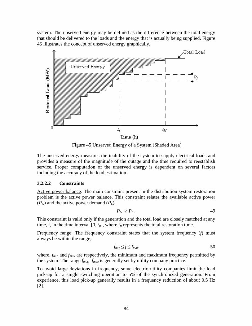
84

system. The unserved energy may be defined as the difference between the total energy that should be delivered to the loads and the energy that is actually being supplied. Figure 45 illustrates the concept of unserved energy graphically.

Figure 45 Unserved Energy of a System (Shaded Area)

The unserved energy measures the inability of the system to supply electrical loads and provides a measure of the magnitude of the outage and the time required to reestablish service. Proper computation of the unserved energy is dependent on several factors including the accuracy of the load estimation.

3.2.2.2 Constraints Active power balance

PG ≥ PL . 49

: The main constraint present in the distribution system restoration problem is the active power balance. This constraint relates the available active power (PG) and the active power demand (PL),

This constraint is valid only if the generation and the total load are closely matched at any time, t, in the time interval [0, tR], where tR represents the total restoration time.

Frequency range

fmin ≤ f ≤ fmax 50

: The frequency constraint states that the system frequency (f) must always be within the range,

where, fmin and fmax are respectively, the minimum and maximum frequency permitted by the system. The range fmin, fmax is generally set by utility company practice.

To avoid large deviations in frequency, some electric utility companies limit the load pick-up for a single switching operation to 5% of the synchronized generation. From experience, this load pick-up generally results in a frequency reduction of about 0.5 Hz [2].

85

Single switching constraint

: It is of general interest to prevent feeders from being energized and de-energized at multiple occasions during the restoration process. In this regard, the single switching constraint establishes that once a feeder is online it must remain online for the remainder of the restoration process. This constraint can be stated as

( ) ( )+− ≤ tutu ii 51

where, u is the status of the ith feeder. The status of the feeder is a binary variable where 1 represents energized feeders and 0 de-energized feeders. t- and t+ represent respectively the time before energization and after energization of the feeder. It is conjectured that there may be cases in which Equation ( ) ( )+− ≤ tutu ii 51 might be relaxed allowing de-energization of feeders after being restored.

Reactive power balance

QG ≥ QL . 52

: The reactive power balance may be implemented to guarantee an acceptable system operation. This constraint establishes that the reactive power (QG) available in the proximity of the feeder to be energized must be equal to the reactive power demand (QL) under adverse conditions. This constraint is critical when energizing feeders with induction motors as high levels of reactive power may be required. A perfect balance should produce an adequate voltage profile. The typical reactive power balance constraint may be defined as,

Voltage profile limits

: The voltage profile constraint makes sure that voltages throughout the distribution system will remain within the desired range as a result of load restoration. This ensures that the load to be energized will not result in an undesired temporary or permanent voltage profile. An unacceptable temporary voltage profile may be a result of inrush current due to motor starting, loss of diversity in loads, or capacitor switching. The voltage range is generally defined as,

maxminVVV i ≤≤ 53

where iV is the magnitude of the voltage at bus i, min

V and max

V are respectively, the minimum and maximum voltage magnitudes needed to guarantee acceptable system operation.

3.2.3 DSR Formulation for Integer Programming

The DSR problem described in Equation ( ) ( )∑=

=FN

iiiiUE ttPtCC

1

46 through

Equation maxmin

VVV i ≤≤ 53 is not in standard form for integer programming implementation. To convert the DSR problem into integer programming form, one

necessary step is to replace the decision variable t of Equation ( ) ( )∑=

=FN

iiiiUE ttPtCC

1

46 with another decision variable x, of binary nature, that represents the status of the feeder. The conversion is possible by breaking the time horizon into several time intervals NT. At each interval, there will be a binary variable for that feeder and the

86

purpose is to determine the corresponding feeder status. The equivalent to Equation

( ) ( )∑=

=FN

iiiiUE ttPtCC

1

46 in its integer programming form is as follows,

( ) ∑∑= =

=T FN

t

N

itititi xPCxF

1 1,,, . 54

Note that this conversion increases the number of variables from NF to NF × NT as the status is indicative of both the feeder and the time interval. Note that { }1,0, ∈tix . To reduce the problem dimension, it is generally desired to limit the number of time intervals used. However, limiting the number of time intervals, compromises the quality of the solution as the more time intervals generally lead to a more detailed restoration plan.

In addition to the variable replacement, the feeder cost function C and load function P that are present in the objective function are also modified to remove their time dependency. In this regard, the values of C and P are replaced by a set of coefficients that are indicative of the corresponding value in each interval and for each feeder. These coefficients, when possible, are computed prior to the optimization process in an effort to speed up execution time. Figure 46 illustrates how the cost coefficients are obtained for the integer programming form. Note that the selected cost coefficient is the average of the extreme points of the interval.

Figure 46 Cost Function for the ith Feeder Based on a Four-Period Horizon

In some cases, computation of the P function for the integer programming formulation may be done in a similar way to Figure 46. However there are cases, such as the cold load pickup transient, where the computed coefficients may not represent adequately all system conditions. For these conditions, artificial variables may be required to model the time varying characteristics of feeders. This will be discussed later in Section 3.2.4.4.

87

Time dependent constraints such as the power balance are treated in a similar way as the cost function conversion shown in Figure 46. When the horizon is broken down in time intervals, a power balance constraint is assigned to each time interval based on the expected available generation curve that serves as an input to the algorithm (Figure 47).

Figure 47 Power Balance Equations Based on a Four-Period Horizon

For the single switching constraint, once a feeder has been energized at some time interval T, the status of the feeder must remain the same for the following time intervals. This is formulated as follows,

TNiTiTi xxx ,1,, ... ≤≤≤ + . 55

Other approximations to the single switching constraint may also be used. An alternative that considers this constraint as part of the objective function will be presented in Section 3.3.2.

3.2.4 Cold Load Pickup in Distribution System Restoration When dealing with a restorative state, the typical pattern followed by loads during normal operation is disrupted. Understanding how feeders will behave after a blackout and predicting how much load will be present at a feeder at the moment of restoration may be very complex. This is a result of the number of factors that play a part in the feeder load. As examples:

• A number of loads within a feeder may trip due to the interruption requiring manual restoration.

• A large amount of reactive power may be drawn from the grid temporarily due to motor starting.

• Thermostatically controlled loads may operate at once in an effort to comply with the desired control settings.

• Typical user pattern may be altered prompting a non-standard behavior.

88

The set of issues that affect load estimation and behavior during restoration are generally referred to as cold load pickup (CLPU). Several industry practices are generally used to estimate the CLPU characteristics of feeders. Common approaches include:

• Relating a feeder to other feeders that are similar in nature.

• Estimating the CLPU characteristic by analyzing the behavior of the feeder in previous outages [18].

The CLPU issues that affect load estimation may be classified further based on their nature. For example, some loads are sensitive to external factors such as weather and outage duration while other loads react transiently based on their intrinsic nature. In some cases, the service interruption may affect some loads inconsistently, making their presence in the feeder uncertain. Based on these characteristics, a classification within CLPU may be extended to: loss of diversity, inherent transient behavior and uncertainty. Note that, for each feeder, all three groups may be present at the same time in a composition that may be unique to that feeder, leading to a specific CLPU characteristic.

3.2.4.1 Loss of Load Diversity During normal operation, not all of the loads connected to a feeder may operate at the same time. Due to this, the maximum demand registered at a feeder is generally less than the sum of the maximum demands of each individual load. This concept is known as diversified demand or maximum coincident demand [87].

During outages, the load composition of some feeders may affect the diversified demand. For some loads, such as thermostatically controlled loads, the probability of a load operating, once the feeder is restored, is dependent on the outage duration and other external factors. A common pattern shown by feeders dominated by loads such as thermostatically controlled loads is to register an increase in their diversified demand as the outage duration increases. Once the feeder is restored, diversity is slowly regained, lowering the diversified demand. An example of this concept is illustrated in Figure 48.

Three regions are shown in Figure 48: pre-interruption, interrupted service and restored service [82]. During the interruption, the load supplied to the feeder drops to zero due to the absence of the electrical service. However, the estimated load value at the feeder increases as the diversity in the loads is lost. When the service is restored, diversity is progressively regained resulting in a reduction of the load being supplied by the feeder. Note that the maximum load due to loss of diversity is dependent on the duration of the interruption and may be as much as the sum of their maximum demands. Also, the shorter the interruption duration, the smaller the load peak registered at the feeder.

89

Figure 48 An Example of Power Demand Illustrating Loss of Load Diversity

3.2.4.2 Inherent Transient Behavior Inherent transient behavior relates to how loads will react once they are energized. The transient behavior of loads is predominantly governed by internal factors rather than external factors as in the case of loss of load diversity. A well known case is the inrush current phenomena seen in magnetic devices such as motors and transformers [31]. For example, when starting an induction motor, the current drawn by this load may be several times the full load current. In addition, at motor starting, the reactive power is the dominant component decaying to its nominal value as the motor accelerates towards rated speed (Figure 49). Predominantly resistive loads show relatively constant values and may be modeled adequately by step functions of real and reactive power.

90

Figure 49 Example of Cold Load Pick-up Transient as a Function of Time

When energizing a feeder, it is necessary to account for the inherent transients of loads. As an example, energizing one or more feeders with a large component of induction motors may result in an undesired voltage drop in the system due to the reactive power requirement.

3.2.4.3 Load Uncertainty Load uncertainty is closely related to loss of load diversity and transient behavior. It takes into account variations in load estimation due to other factors such as: involuntary tripping of loads, disrupted patterns in user behavior or manual motor starting plans. Feeders whose load is easier to predict, that is, have historically exhibit a low deviation from the estimated value, are more favorable for early restoration. Feeders that have a large deviation from the estimated value may be restored at a later stage in an effort to prevent undesired system operation. In this context, historical data may be used to calculate a probability index or other sort of measure that captures the uncertainty of a feeder. Figure 50 is an illustrative example of this concept. The better the estimation (e.g. smaller deviation) the more favorable it is for early restoration.

91

Figure 50 Pictorial of Uncertainty in Feeders

3.2.4.4 CLPU Modeling As stated earlier in Section 3.2.4 the CLPU characteristic of each feeder may be specific to that feeder as a result of load composition. In residential feeders, a typical behavior for the cold load pickup is that of an exponentially decaying function similar to the one shown in Figure 51 [60]. Industrial and to certain extent commercial feeders show a different behavior. Some studies [88] suggest a steadily increasing CLPU characteristic for predominantly industrial feeders. This may be attributed to the load restoration plans performed within an industry. This case is also illustrated in Figure 51.

Figure 51 Common Types of CLPU Transients (After [60], [88])

The most common CLPU model used is a time varying function of the form [89],

( ) ( ) ( )[ ] ( ) ( )[ ] ( )122 12 ττττα −−−+−−+= −− tutuPtuePPPtP Ut

DUD 56

92

where PD is the diversified load, PU the undiversified load, τ1 the time at which the restoration begins, τ2 time at which the load diversification begins, α is the rate of decay of the load and u(t) a unit step function.

The nonlinearity associated with this CLPU formulation restricts the optimization methods that may be used. Some approaches such as analytic methods [90], genetic algorithms [82] and ant colony [91] have been suggested for developing restoration plans with CLPU. However, for large scale systems, the application of these methods may be limited due to computational requirements.

Modeling the CLPU phenomena as a linear combination of variables may be achieved by partitioning the function into power levels and time intervals. The most relevant blocks along with their time constants may be selected to model an approximation of the CLPU phenomena. This will be referred from this point forward as block decomposition and an illustration of it is shown in Figure 52.

Figure 52 Cold Load Pickup Model through Load Decomposition

By decomposing the load into several blocks, the block decomposition converts the nonlinear function into a summation of the form,

∑=

+=B

k

N

ktkTRtSSt yPxPP

1, 57

where PSS is the steady state load value of the ith feeder, PTRk is the transient load peak value of block k and NB represents the number of blocks selected for modeling.

The presence of the block in the time interval t, is controlled by the variables x and y. The variable x is the status of the feeder and determines the instant in which the load should be restored. The yk variable controls the kth block that is used to model the transient. This variable is dependent on the value of x and a time constant that establishes the duration of the kth block. The dependent variable yk is active (e.g. yk = 1) if the steady state block has not been energized for longer than the corresponding transient time constant. The variable becomes inactive (e.g. yk = 0), when the steady state block has been energized

93

for a time that is longer than the transient time constant. The complete set of rules that govern the dependent variable y are shown as follows,

( )( )

≤−=>−=

==

kti

kti

ti

ti

ttxttx

xy

ττ

0,

0,

,

,

and1,1and1,0

0,0 58

where, τk is the time constant of block k and t0 is the restoration time of the load (e.g. the time when the variable x goes from deenergized to restored).

For purposes of this development, a two block load is used to represent the CLPU model. The first block represents the steady state load of the feeder while the second block is used to represent the transient characteristics of the CLPU phenomena. Although the use of more blocks emulates better the CLPU transient, there is a computational advantage of modeling loads with the least amount of blocks. In addition, two blocks may be desired by utilities during restoration as it may lead to a more conservative scenario. Figure 53 illustrate the CLPU model used in this development.

Figure 53 A Model for Cold Load Pick-Up in Distribution Restoration

3.2.5 Unit Commitment and Distribution Restoration Duality The generation unit commitment problem (UC) and the distribution system restoration problem (DSR) have, for many years, occupied the attention of electric power engineers. While these two power engineering problems are very diverse, spanning the spectrum of power engineering from sources to loads, they do share some common attributes. The UC and DSR are constrained optimization problems which may, in fact, be considered as duals of each other [50]. The term dual refers to problems in which key parameters in one problem have a cognate in the other problem. In addition, the models within each problem are virtually identical in form to the other problem. A discussion of duals in electric circuit theory is presented in DeCarlo and Lin [92].

One value of duality is that the computational methods developed for a given problem, and efforts expended on solving that given problem, may be applied to the dual of that problem. In this case, the extensive effort and engineering that have gone into the

94

efficient solution of the unit commitment problem, including solutions of large systems, might be applicable to the solution of the distribution system restoration problem.

3.2.5.1 Key Parameters in the UC and DSR Problems The power systems unit commitment finds the set of generators that must be online, with the goal of serving the system load optimally over a given time horizon. The basic UC problem minimizes the production cost (e.g. running, start up, and shut down costs) associated with power plant operation. This production cost is optimized by determining the adequate unit status (online or offline) for the time horizon under study. Typical constraints of the UC problem include: the system power balance, system requirements such as spinning reserve and physical limitations of the generating units including ramp rate limits, minimum running time and start up / shut down characteristics.

The solution of the DSR problem is less clear even for the simple case of only radial distribution feeders. There have been a large number of conceptual studies suggested in the solution of this problem. A common approach used is to restore the system by minimizing the system outage cost or alternatively the system unserved energy. This approach requires the operators to decide which feeders to energize and when to perform this action. The DSR problem finds the status of each feeder (energized or deenergized) over the desired time horizon. Common constraints used in this problem are: power balance, frequency deviation limits, reactive power requirement, and transient behavior, among others.

From both problems, it can be seen that the goal is to determine the appropriate status for each decision variable (generators or feeders) while meeting the system requirements (e.g. load or generation) and other constraints. Furthermore, the selection of the decision variable is done by minimization of the related cost over a given time horizon (e.g. production cost in UC or outage cost in DSR). Figure 54 illustrates the basic connection between the UC and the DSR problem.

To show the corresponding similarities between both objectives functions, a general formulation of the problem is also included in Figure 54. SU and SD are the startup and shutdown costs of generators or feeders while OC represents the operating costs in UC or outage costs in the DSR problem. The superscript/subscript F, G stands for feeder or generator respectively. Although listed, the startup cost of the DSR problem is generally neglected or used as a negative cost when dealing with loads of high priority. A list of the basic parameters present in the UC and DSR problems is shown in Table 32.

95

Figure 54 UC and DSR Similarities

Table 32 Basic UC and DSR Dual Parameters

UC PROBLEM DSR PROBLEM General

operating states

Time Time Generation Load Unit status* Feeder status*

Solution parameters

Time to commit or decommit* Time to energize or deenergize*

System load at time t Available generation from grid at time t Operating cost over time

horizon Cost of unserved energy over restoration

process Generation committed Total connected feeder ratings

*Control variable

3.2.5.2 Solution Methods Over the years, the UC problem has received a lot of attention due to its importance to system operation. Many solution methods have been proposed for the solution of the UC problem in an effort to enhance solution quality and algorithm performance. Two in particular, have been used extensively in the industry, these being: dynamic programming and Lagrangian relaxation.

96

Dynamic programming (DP) is a robust tool for global optimization developed by Richard Bellman in the 1950s [93]. DP decomposes the problem into several stages (or subproblems) and optimizes the solution of these subproblems. The optimal solution to the problem is the best combination of these optimal subpolicies. DP provides several advantages over other optimization techniques, being the most noteworthy the ability to find global optimal solutions to problems. In addition, since DP is not based on differentiation, it is capable of solving problems with a non-continuous solution space such as the case of integer or discrete variables [90]. The main drawback of DP is that it becomes computationally intensive when the number of decision variables is high. For example, a UC study for a large number of generating units over a long time horizon may be unsolvable when using DP. This issue is known as the curse of dimensionality [93].

This limitation has been addressed in part by the use of Lagrangian relaxation (LR). The LR technique finds the solution to a relaxation of the original (primal) problem by adding Lagrange multipliers along with the complicating constraints to the original objective function, f(x). The resulting problem is generally referred to as the Lagrangian dual and its solution consists of a decomposition of the original problem into two subproblems which are easy to solve. One subproblem finds the optimum set of Lagrange multipliers while the other deals with finding the optimum set of decision variables. Due to its capability of handling large scale systems, the LR method has been the preferred method in recent years, for the solution of the UC problem.

The suggested duality between UC and DSR should allow solution of both problems by nearly identical mathematical and computational approaches. An important characteristic of the DSR problem is that it may become very large due to the large number of feeders and time intervals that may be required to represent the problem adequately. The large-scale capabilities of LR indicate this technique may be well suited for solving the DSR problem. For example, the LR technique provides good computational performance with a nearly linear execution time as the problem dimension increases. This computational advantage is shown in [95] by comparing LR to a state of the art branch and cut algorithm, both used for solving the UC problem.

97

3.3 Lagrangian Relaxation Based Distribution Restoration

3.3.1 Relaxations, Duality and Lagrangian Relaxation In optimization theory, especially for large scale problems, solution to some problems may be very difficult to obtain in their standard form. A common approach used to solve these problems is to deal with alternative formulations that are easier to solve, obtaining a feasible bound to the original problem and, if possible, refining the solution towards the global optimum. These easier problems are generally referred to as relaxations.

A problem is said to be relaxed when the original and by definition, difficult problem, is replaced by a simpler problem which will give a solution that is close to or the same as that of the original problem. One type of relaxation may be performed by changing the set of constraints that define the feasible solution space, allowing optimization over a larger set and resulting in a potentially easier problem. These types of relaxations that are performed by changing the set of constraints are referred to as primal relaxations or primal bounds. However, in some cases, finding feasible solutions of good quality for the primal bound relaxations may be as difficult as in the original problem.

Another approach used is based on the duality properties of optimization problems. When good dual formulations are possible, the problem may be transformed into a simpler problem by replacing its objective function or other characteristics with other ones. This new formulation will lead to results that are optimal or near optimal when compared to the original problem. Dual problem relaxations provide a clear advantage over primal problem relaxations in that any dual feasible solution is an upper bound to the primal problem [96]. For relaxations not based on dual formulations, the relaxation may need to be solved to optimality to provide a feasible bound [96].

Figure 55 Illustrative Concept of Relaxation

98

A well known dual formulation is the Lagrangian dual also known as Lagrangian relaxation (LR). The LR technique finds a lower (or an upper) bound to a combinatorial optimization problem by incorporating the complicating constraints into the objective function and relaxing them with the help of Lagrange multipliers. The concept of Lagrange multiplier theory was originally developed by Lagrange in the XVIII century. Perhaps one of the first applications of the LR method in combinatorial optimization was conducted by Held and Karp in the 1970s in an effort to solve the traveling salesman problem [97].

For a combinatorial optimization problem of the form,

min ctx 59

subject to the set of constraints

Ax ≥ b 60

{ }1,0∈x 61

where x is the set of decision variables of the problem, c is the vector of coefficients of the objective function, A is the matrix of coefficients for the problem constraints and b is the vector of right hand side terms of the constraints, the concept of Lagrange relaxation is to bring the set of constraints Ax ≥ b 60 into the objective function. In this case, this means the formulation of a new function L(x,λ),

( ) ( )AxbxcxL tt −+= λλ, . 62

The function L is now viewed much like a Lagrangian as in the optimization method of Lagrange multipliers.

The LR method decomposes the given problem into two smaller optimization problems. One problem (the outer problem) deals with optimizing the set of Lagrange multipliers λ, while the other (the inner problem) optimizes the decision variables x of the original problem. In this context, the resulting structure of the Lagrangian dual problem is as follows,

( )λλ

,minmax xLx

63

where the Lagrangian dual problem is a function of the set of binary variables x in constraint { }1,0∈x 61and the Lagrange multipliers. Proper implementation of the method requires the Lagrange multipliers to be non-negative values, that is, 0≥λ . In some cases, it may be useful to consider some constraints as part of the inner problem optimization block instead of being included as part of the Lagrangian [98]. References [98–100] provide more detail related to this technique and its implementation. Alternatively, a min max formulation may also be used depending on the problem characteristics.

The solution to the Lagrangian dual is computationally easier to obtain than the original problem and for this reason is a popular method when dealing with large scale systems. Due to the nature of dual formulations, there may be a difference between the primal and the dual problem objective values. This difference is commonly referred to as the duality gap. The duality gap and its existence are dependent on the characteristics of the

99

problem. In some cases, the dual solution may equal the solution of the primal problem, this being called strong duality. In the same context, a weak duality condition happens when the solution (bound) obtained by the dual problem is worse than the solution of the primal problem. This is a consequence of the constraints that are neglected during the solution of the dual [101]. To address the issue of a weak duality condition, augmented Lagrangian functions have been suggested [99] that reduce the duality gap through the use of penalty functions. Note that the inclusion of a penalty function has attendant problems, for example, heuristic selection of the function. In addition, some approaches to estimate the duality gap have been proposed [102].

3.3.2 LR Based Distribution System Restoration Solution to the distribution restoration problem via Lagrangian relaxation requires the time horizon to be broken into several time intervals as indicated in Section 3.2.3. At each time interval, the purpose is to determine the status (either online or offline) of all the feeders present in the restoration process. In this context, the total number of decision variables is dependent on the number of feeders times the number of time intervals.

One way to formulate the Lagrangian dual of the distribution restoration problem is to include the active and reactive power balance constraints into the objective function

through Lagrange multipliers ( ( )

++ ∑∑

==

TT N

ttBtQ

N

ttBtPx

QPxF11

minmax λλλ

. 64),

( )

++ ∑∑

==

TT N

ttBtQ

N

ttBtPx

QPxF11

minmax λλλ

. 64

In this development, the single switching constraint shown in Equation ( ) ( )+− ≤ tutu ii

51 is replaced with a shutdown cost added to the objective function

( ( ) ( )( )( )∑∑= =

+−+=T FN

t

N

itititiitititi xxxxPCxF

1 11,,,,,, ω . 65). This corresponds to the

second term shown in ( ( ) ( )( )( )∑∑= =

+−+=T FN

t

N


1 11,,,,,, ω . 65),

( ) ( )( )( )∑∑= =

+−+=T FN

t

N


1 11,,,,,, ω . 65

The frequency constraint is neglected by assuming that sufficient generation has been synchronized to the system prior to the distribution restoration stage. The constraints present in the LR based distribution restoration formulation are as follows,

Tti

N

iitGtB NtxPPP

F

,...,1,,1

=−= ∑=

66

Tti

N

iitGtB NtxQQQ

F

,...,1,,1

=−= ∑=

67

{ } TFti NtNix ,...,1,,...,1,1,0, ==∈ 68

100

0≥Pλ , 0≥Qλ , { }QP λλλ ,= 69

where NT is the number of time intervals of the discretized restoration problem, Ci,t and Pi,t are respectively the cost and estimated load for the ith feeder at time interval t, ωi represents the cost of turning off the ith feeder after being energized, λP and λQ are respectively, the set of Lagrange multipliers for the P and Q inequality constraints, λ is the total set of Lagrange multipliers and xi,t is the status of the ith feeder at time interval t. The feeder status is a binary variable with a value of 0 for de-energized feeders or 1 for

energized feeders. Note that in ( ( )

++ ∑∑

==

TT N

ttBtQ

N

ttBtPx

QPxF11

minmax λλλ

. 64) a max min

approach is used instead of a min max formulation because of the adopted 0, 1 feeder status convention. PBt and QBt are the power balance constraints at interval t. In Equations

Tti

N

iitGtB NtxPPP

F

,...,1,,1

=−= ∑=

66 and Tti

N

iitGtB NtxQQQ

F

,...,1,,1

=−= ∑=

67, the equality sign is used for simplicity of notation in Equation

( )

++ ∑∑

==

TT N

ttBtQ

N

ttBtPx

QPxF11

minmax λλλ

. 64 and does not represent an equality

constraint.

Figure 56 illustrates the Lagrangian relaxation algorithm with subgradient iterations for load restoration. The algorithm parameters µ (step length), α (convergence factor), iter (maximum number of iterations without improvement to the bound) and Zub (upper bound) control the convergence characteristics of the algorithm. Typical values for µ and α in distribution system restoration problems are 2 and 0.5 respectively.

3.3.2.1 The Outer Problem and the Subgradient Iteration Method Part of the LR solution is the search for the parameters λ. This may be done by a brute force search allowing λ values to span a reasonable range – and simply search for the solution to ( ( ) ( )AxbxcxL tt −+= λλ, . 62) – ( ( )λ

λ,minmax xL

x 63). Note that

when the constraint Ax ≤ b is of dimension m, λ is also of dimension m. Therefore, the brute force scan of values of λ is not computationally efficient for large m. For this reason it is expedient to study the use of a gradient of the function L with respect to λ. This technique is called a subgradient iterative technique. The subgradient iterative technique is an optimization method used mainly for non-differentiable functions developed by Shor in the 1970s [100]. The method is a generalization of other gradient based methods and it is often applied in conjunction to primal / dual formulations to obtain a relatively simple iterative optimization algorithm.

101

Set k = k + 1

Compute λ(k) via subgradient iterationsInput: x(k-1), λ(k-1), Zlb

(k-1)

Output: λ(k-1)

Solve inner problemInput: λ(k)

Outputs: x(k), Zlb(k)

Set k = 0 and j = 0Set Zbb = - inf

Estimate initial λ(k)

System data: A, b, fAlgorithm: µ, α, Zub, Iter

Zlb(k) > Zbb

xopt = x(k)

λopt = λ(k)

Zbb = Zlb(k)

Convergence/Termination criteria

reachedEnd

Yes

No

Yes

j = Iter

µ = µ*αj = 0

j = j + 1

Yes

No

No

Figure 56 LR Algorithm with Subgradient Iterations

In the Lagrangian relaxation method, the subgradient iterative technique is commonly used to update the set of Lagrange multipliers λ. The general procedure, at iteration k is,

102

( ) ( )1−−= kk Axbg 70

( )( )

( )2

1

k

klbubk

gZZ −−

= µγ 71

( ) ( ) ( ) ( )( )kkkk g γλλ += −1,0max 72

where A is a m x n matrix; λ, g and b are m dimensional column vectors; x is an n dimensional column vector and γ, μ, Zub, Zlb are scalars. This computation requires an estimate of the Lagrange multipliers at the initial iteration, λ(0), along with the calculated bound, ( )0

lbZ , and decision variables, x(0), that result from the solution of the inner problem. The updated set of Lagrange multipliers obtained through ( ( ) ( )1−−= kk Axbg 70) – ( ( ) ( ) ( ) ( )( )kkkk g γλλ += −1,0max 72) is used to compute a new bound and the corresponding values of the decision variables. The advantages of the subgradient search include high speed and no large requirements for storage of data. In contrast, the subgradient may have convergence issues for certain problems.

3.3.2.2 The Inner Problem and the Restoration Index

By rearranging Equation ( ( ) ( )AxbxcxL tt −+= λλ, . 62), it can be seen that the Lagrangian dual can be reformulated as

( ) ( ) bxAcxL tt λλλ +−=, . 73

Solution to the inner problem is obtained by optimizing the problem

( )( )k

xAc t

x λλλ

=−min 74

subject to { }1,0∈x .

Due to the binary nature of the decision variable, solution to the inner problem can easily be obtained by computation of the coefficient ( )Ac tλ− . If the coefficient has a negative sign the function is maximized when the decision variable adopts a value of 0. For coefficients with a positive sign, a value of one maximizes the function. When a coefficient has a value of zero, the value of the variable is undetermined as it can be either 0 or 1. Heuristics are commonly used to solve these states and determine the feasible solution of the problem. For purposes of the proposed operator-permissive algorithm, this status is labeled as operator discretion. The operator discretion status is for feeders that are near restoration. In this case, the operator may elect to restore or delay restoration of those feeders, based on the actual state of the system or personal experience making sure that all the system requirements are satisfied. This is shown in

(( )( )( )( )

( )( )

=−<−>−

=0,

0,10,0

AcODAcAc

xk

k

k

λλλ

. 75)

103

( )( )( )( )

( )( )

=−<−>−

=0,

0,10,0

AcODAcAc

xk

k

k

λλλ

. 75

For the optimal solution of the Lagrangian dual, the coefficient ( )Ac tλ− serves as a measure of how favorable it is to energize a feeder. The closer this coefficient is to zero the more likely it is for that feeder to change status (from OFF to ON or vice-versa if allowed by the operator). The farther it is from zero, the more likely it is to remain at its current status. This coefficient can be referred to as the restoration index. An important note is that computation of the restoration index in this development does not consider

the shutdown cost term shown in ( ( ) ( )( )( )∑∑= =

+−+=T FN

t

N


1 11,,,,,, ω 65).

3.3.3 Distribution Restoration Infrastructure During system operation, a system perturbation may cause an outage forcing the system to move away from its original state called the normal operation state to a new state which may be referred to as the restorative state. Some of these states are illustrated in [103]. The magnitude of the perturbation will determine the combination of system components that are affected (e.g. generators, transmission lines and loads) and consequently the severity of the outage. The restoration process works to restore these components. During the first stages of the restoration process, the operator goal is to stabilize the system parameters and restore the main transmission grid. Once the objective has moved from providing suitable conditions for load restoration to minimizing the outage impact, then the proposed restoration algorithm may be applied. For illustration, the suggested states of the system during restoration are depicted in Figure 57.

Figure 57 General Overview of the Restoration Process

104

The suggested Lagrangian relaxation restoration algorithm is devised to be executed every few minutes in parallel to the distribution restoration process obtaining a solution that should be valid for a given time horizon. This simultaneous computation should present the operator with a set of options that may be used to restore the system. This algorithm is of the permissive type, intended to constantly interact with the operator in the restoration process. However, decision-making is still performed by the operator based on several criteria and personal experience.

Interaction is carried out by first creating a master plan based on initial estimates of the system. As the distribution system is restored and adjustments to the master plan are required, the algorithm should update the plan based on the remaining part of the system to be restored. This concept is illustrated in Figure 58.

Figure 58 Guided Restoration of Distribution Systems

The solid line represents the original restoration plan returned by the restoration algorithm. The lines marked with black rhombus and white circles represent the alternative restoration plans that are needed at t1 and t3 respectively to account for deviations from the original restoration plan. The impact of available generation changing in real time is illustrated by three characteristics: an original plan, an adjusted plan on the basis of changed generation availability, and a second adjusted plan.

Algorithm performance varies with the system (or island) dimension. However, general computational times should lie in what is called operational real time. Common time frames for operational real time are in the order of seconds to a few minutes. Figure 59 shows a diagram that illustrates the concept of operational real time within power systems. It is of importance to note, that the restoration plan and its accuracy is a function of the load and generation estimation that serve as input data.

105

Figure 59 Power System Time Frames

3.3.4 An Evolutionary Computation Heuristic for the Outer Problem For validation purposes, and also in the solution of some restoration problems in which the subgradient iteration method may present convergence problems, the use of heuristics may be useful for obtaining the set of Lagrange multipliers. Families of heuristics that may be used when involving non-differentiable problems such as the case of distribution restoration are evolutionary algorithms. Evolutionary algorithms are optimization techniques that solve problems using a simplified model of the evolution process. These algorithms are based on the concept of a population of individuals that evolve and improve their fitness through probabilistic operators like recombination and mutation. These individuals are evaluated in each generation and those that perform better are selected to compose the population in the next generation. After several generations these individuals evolve improving their fitness as they explore the solution space for the optimal value.

Several algorithms have been developed within the field of evolutionary computation being the most studied genetic algorithms, evolutionary programming and evolution strategies. These algorithms were first conceived in the 1960s when evolutionary computation started to get attention. Recently, the success achieved by evolutionary algorithms in the solution of complex problems and the improvements made in computation, such as parallel computation, have stimulated the development of new algorithms like differential evolution, particle swarm optimization, ant colony search and scatter search that present great convergence characteristics and capability of determining global optima. Evolutionary algorithms have been successfully applied to many optimization problems within the power systems with references [104] and [105] providing a good overview of the available literature.

106

3.3.4.1 The Differential Evolution Optimization Algorithm Differential Evolution (DE) is an optimization algorithm that solves real-valued problems based on the principles of natural evolution [106-107]. It uses a population of PN floating point encoded individuals (candidate solutions) that evolve over G generations to reach an optimal solution. Each individual, or candidate solution, is a vector that contains as many parameters ( ( ) ( ) ( ) ( )( ) P

Gc

Gb

Ga

Gi NiXXFXX ,...,1, =−+=′ 77) as the

problem decision variables D.

DE creates new offsprings by generating a noisy replica of each individual of the population. The individual that performs better from the parent vector (target vector) and the replica (trial vector) advances to the next generation. This optimization process is carried out with three basic operations: Mutation, crossover and selection. First, the mutation operation creates mutant vectors by perturbing each target vector with the weighted difference of two other individuals selected randomly. Then, the crossover operation generates trial vectors by mixing the parameters of the mutant vectors with the target vectors, according to a selected probability distribution. Finally, the selection operator forms the next generation population by selecting between the trial vector and the corresponding target vector those that fit better the objective function.

3.3.4.2 The Differential Evolution Optimization Process The first step in the DE optimization process is to create an initial population of candidate solutions by assigning random values to each decision parameter of each individual of the population. Such values must lie inside the feasible bounds of the decision variable, and can be generated by using

( ) ( )min max min, , 1,..., ; 1,...,j i j j j j PX X X X i N j Dη= + − = =0 76

where minjX and max

jX are respectively, the lower and upper bound of the jth decision parameter (in this case the Lagrange multiplier) and jη is a uniformly distributed random variable within [0, 1] generated anew for each value of j. After the population is initialized, it evolves through the operators of mutation, crossover and selection. The mutation operator is in charge of introducing new parameters into the population. To achieve this, the mutation operator creates mutant vectors by perturbing a randomly selected vector (Xa) with the difference of two other randomly selected vectors (Xb and Xc). All of these vectors ( ( ) ( ) ( ) ( )( ) P

Gc

Gb

Ga

Gi NiXXFXX ,...,1, =−+=′

77) must be different from each other, requiring the population to be of at least four individuals (accounting also the trial vector i) to satisfy this condition. To control the perturbation and improve convergence, the difference vector is scaled by a user defined constant in the range [0, 1.2]. This constant is commonly known as the scaling constant (F). An illustration of the mutation operator is shown in Figure 60 A Two-Dimensional Representation of the Mutation Operator.

( ) ( ) ( ) ( )( ) PG

cG

bG

aG

i NiXXFXX ,...,1, =−+=′ 77

107

where Xa, Xb, Xc, are randomly chosen vectors ∈ {1,…, PN } and a ≠ b ≠ c ≠ i . Xa, Xb and Xc, are generated anew for each parent vector. F is the scaling constant.

Figure 60 A Two-Dimensional Representation of the Mutation Operator

The crossover operator creates the trial vectors, which are used in the selection process. A trial vector is a combination of a mutant vector and a parent (target) vector performed based on probability distributions. For each parameter, a random value based on binomial distribution (preferred approach) is generated in the range [0, 1] and compared against a user defined constant referred to as the crossover constant. If the value of the random number is less or equal than the value of the crossover constant the parameter will come from the mutant vector, otherwise the parameter comes from the parent vector (3.20). This allows parameters from parents to be part of future generations. Figure 61 shows how the crossover operation is performed.

Figure 61 Crossover Operator

108

The crossover operation maintains diversity in the population, preventing local minima convergence. The crossover constant ( RC ) must be in the range of [0, 1]. A crossover constant of one means the trial vector will be composed entirely of mutant vector parameters. A crossover constant near zero results in more probability of having parameters from the target vector in the trial vector. A randomly chosen parameter from the mutant vector is always selected to ensure that the trial vector gets at least one parameter from the mutant vector even if the crossover constant is set to zero.

( )( )

( )

===≤′′

=′′ DjNiX

qjCXX PG

ij

RjGijG

ij ,...,1,,...,1,otherwise

orif

,

,,

η 78

where q is a randomly chosen index ∈{1,…,D} that guarantees that the trial vector gets at least one parameter from the mutant vector; jη′ is a uniformly distributed random

number within [0, 1) generated anew for each value of j. ( )GijX , is the parent (target)

vector, ( )GijX ,′ the mutant vector and ( )G

ijX ,′′ the trial vector.

The selection operator chooses the vectors that are going to compose the population in the next generation (iteration). This operator compares the fitness of the trial vector and the fitness of the corresponding target vector, and selects the one that performs better

( ( )( ) ( )( ) ( )( )

( ) PGi

Gi

Gi

GiG

i NiX

XfXfXX ,...,1,

otherwiseif1 =

≤′′′′

=+ 79). The selection process is

repeated for each pair of target/trial vector until the population for the next generation is complete.

( )( ) ( )( ) ( )( )

( ) PGi

Gi

Gi

GiG

i NiX

XfXfXX ,...,1,

otherwiseif1 =

≤′′′′

=+ 79

Variations to the canonical form of the DE algorithm are also available. This variation differs in how the operators of mutation, crossover and selection are implemented. A particular efficient one, which was used for validation purposes in this development, finds the difference of two pair of vectors rather than one. In addition, the best solution found so far, is used to create the subsequent generations. The aforementioned variation is shown in ( ( ) ( ) ( ) ( ) ( ) ( )( ) P

Gd

Gc

Gb

Ga

Gbest

Gi NiXXXXFXX ,...,1, =−+−+=′ 80)

( ) ( ) ( ) ( ) ( ) ( )( ) PG

dG

cG

bG

aG

bestG

i NiXXXXFXX ,...,1, =−+−+=′ 80

where Xa, Xb, Xc and Xd are randomly chosen vectors from the NP population and a ≠ b ≠ c ≠ d ≠ i Xa, Xb, Xc and Xd are generated anew for each parent vector. Xbest is the best solution found so far. This variation Equation

( ) ( ) ( ) ( ) ( ) ( )( ) PG

dG

cG

bG

aG

bestG

i NiXXXXFXX ,...,1, =−+−+=′ 80 replaces Equation ( ) ( ) ( ) ( )( ) P

Gc

Gb

Ga

Gi NiXXFXX ,...,1, =−+=′ 77 in the algorithm. The general steps of the

DE algorithm are shown in Table 33 General Steps of the DE Algorithm.

109

Table 33 General Steps of the DE Algorithm

DE Algorithm 1. Initialize population (76) 2. While convergence criteria are not satisfied 3. Create mutant vectors with the difference vector and the scaling constant (80) 4. Generate trial vectors applying the selected crossover scheme (78) 5. Select next generation members according to competition performance. (79)

3.3.5 Summary This chapter discusses a Lagrangian relaxation approach to the solution of the suggested restoration problem. The main points raised in this chapter are:

• The Lagrangian dual relaxation as a way to simplify difficult problems from combinatorial optimization and obtain optimal or near optimal solutions.

• The subgradient iterations approach as a fast and computationally efficient method for determining the Lagrange multipliers.

• The restoration index as a measure of the feeder restoration status that result from the solution to the inner problem in the Lagrangian decomposition.

• Alternative methods for the solution of the outer problem, when the subgradient iterations method presents convergence problems.

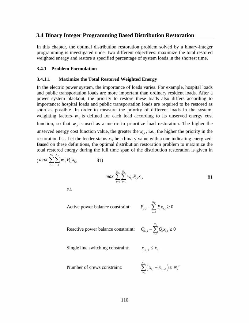
110

3.4 Binary Integer Programming Based Distribution Restoration

In this chapter, the optimal distribution restoration problem solved by a binary-integer programming is investigated under two different objectives: maximize the total restored weighted energy and restore a specified percentage of system loads in the shortest time.


3.4.1.1 Maximize the Total Restored Weighted Energy In the electric power system, the importance of loads varies. For example, hospital loads and public transportation loads are more important than ordinary resident loads. After a power system blackout, the priority to restore these loads also differs according to importance: hospital loads and public transportation loads are required to be restored as soon as possible. In order to measure the priority of different loads in the system, weighting factors- ,i tw is defined for each load according to its unserved energy cost function, so that ,i tw is used as a metric to prioritize load restoration. The higher the unserved energy cost function value, the greater the ,i tw , i.e., the higher the priority in the restoration list. Let the feeder status xi,t be a binary value with a one indicating energized. Based on these definitions, the optimal distribution restoration problem to maximize the total restored energy during the full time span of the distribution restoration is given in

( , , ,1 1

T FN N

i t i t i tt i

max w P x= =∑∑ 81)

, , ,1 1

T FN N

i t i t i tt i

max w P x= =∑∑ 81

. .s t

, ,1

Active power balance constraint: 0FN

G t i i ti

P Px=

− ≥∑

, ,1

Reactive power balance constraint: 0FN

G t i i ti

Q Q x=

− ≥∑

, 1 ,Single line switching constraint: i t i tx x− ≤

( ), , 11

Number of crews constraint: FN

ti t i t c

ix x N−

=

− ≤∑

111

( ), , 1

Number of feeder operations in the

same substation constraint: tt tx x Nκ κ κ

κ−− ≤∑

, 'Specified load restoration constraint: 1j tx ≥

,Binary variable constraint: {0,1}i tx ∈

Compared to the constraints formulated in the previous chapters, there are three new

constraints in ( , , ,1 1

T FN N

i t i t i tt i

max w P x= =∑∑ 81):

• Number of crews constraint: during the distribution system restoration, the number of feeder operations in a given time interval is limited by the number of crews who can execute these operations.

• Number of feeder operations in the same substation constraint: during the distribution system restoration, the number of feeder operations in the same distribution substation will be limited by protection settings.

• Specified load restoration constraint: during the distribution system restoration, some loads may be required to be restored no later than some specified time point. For these loads, their status at the specified time interval should be “1”.

The BIP problem ( , , ,1 1

T FN N

i t i t i tt i

max w P x= =∑∑ 81) is solved by Branch-and-Cut method,

which is a hybrid of Branch-and-Cut and Cutting Plane methods. The factors affecting the algorithm efficiency include the number of variables NV and the number of constraints Nc as well as the variability of the objective function (i.e., this allows the possibility of early pruning of the tree and can improve average performance). The number of variables NV will decide the number of possible binary variable status and hence the number of nodes (subproblems) to be solved. Let Ns be the number of binary variable status, then

2 2V T FN N NsN ×= = 82

The number of constraints Nc will decide the number of branches that can be cut off for the Branch-and-Cut method.

Based on the above analysis, it is known that key factors affecting the BIP efficiency are the number of time intervals NT, the number of feeders NF and the number of constraints Nc. Thus, we want to increase Nc and decrease NT for a given system where NF is fixed. For a given optimal distribution restoration problem, the parameter can be adjusted in the

optimization problem ( , , ,1 1

T FN N

i t i t i tt i

max w P x= =∑∑ 81) is simply NT. For a BIP problem with

NT time interval and NF feeders, decreasing one time interval will decrease the total number of binary variable status by ΔNs, where it equals

112

( )( 1) ( 1)2 2 2 2 1T F T F T F FN N N N N N NsN × − × − ×∆ = − = − 83

For any practical system, a decrease in the time interval will tremendously decrease the total number of binary variable states in a BIP problem. For example, for a system with NT =20 and NF =100, if NT is decreased by 1, then the number of binary variable states will decrease 22000 as in ( ( )(20 1) 100 100 (20 1) 100 100 20 100 20002 2 1 2 2 2 2sN − × − × ×∆ = − ≈ × = =

84).

( )(20 1) 100 100 (20 1) 100 100 20 100 20002 2 1 2 2 2 2sN − × − × ×∆ = − ≈ × = = 84

The tradeoff of this kind of treatment is the solution may be suboptimal compared to the full problem specification. One is effectively placing a time horizon at each of step of the restoration process in order to improve the computation speed, which is probably the more important concern in the distribution system restoration. The flowchart for this methodology is given in Figure 62 Flowchart of BIP Based DSR with a Moving Time Horizon.

3.4.1.2 Restore a Specified Percentage of System Load in the Shortest Time In 3.4.1.1, the object of optimal distribution system restoration (DSR) problem is formulated to maximize the total restored weighted energy, i.e., minimize the total unserved energy cost, during the full time span of the distribution restoration, which is solved by BIP. In this part, a different objective, restoring a specified percentage k% (0<k≤100) of system load in the shortest time for the DSR problem, is investigated.

The problem to restore k% system load in the shortest time can be described as an “If-

Then-Else” problem as in (

,1

%

1 0

FN

i i t Si

t

t

If Px k P

Then yElse y

=

≥

= =

∑ 85). First, we derive how to

convert the If-Then-Else to equivalent inequality constraints, and then formulate a BIP problem subject to these kinds of constraints.

,1

%

1 0

FN

i i t Si

t

t

If Px k P

Then yElse y

=

≥

= =

∑ 85

113

The “If-Then-Else” problem (

,1

%

1 0

FN

i i t Si

t

t

If Px k P

Then yElse y

=

≥

= =

∑ 85) is equivalent to an

“Either-Or” problem (Either ,1

% 0

1

FN

S i i ti

t

k P Px

y=

− ≤

=

∑ Or ,1

% 0

0

FN

S i i ti

t

k P Px

y=

− >

=

∑

86)

Either ,1

% 0

1

FN

S i i ti

t

k P Px

y=

− ≤

=

∑ Or ,1

% 0

0

FN

S i i ti

t

k P Px

y=

− >

=

∑ 86

114

Figure 62 Flowchart of BIP Based DSR with a Moving Time Horizon

N

N

N

Y

Y

Y

Start

Set number of time point Ntf looking into the future

Current time point t=1

Formulate the BIP problem from t to t+ Ntf -1

Take the results at last time point as the lower bound t>1

Solve the BIP problem

Converged

STOP

t=t+1

Save the solution at t

Last time point

115

If an arbitrary large positive number M is defined compared to Ps, problem (Either

,1

% 0

1

FN

S i i ti

t

k P Px

y=

− ≤

=

∑ Or ,1

% 0

0

FN

S i i ti

t

k P Px

y=

− >

=

∑ 86) can be converted to the

equivalent constraints in (,

1

,1

% (1 )

%

F

F

N

S i i t tiN

S i i t ti

k P Px M y

k P Px My

=

=

− ≤ −

− > −

∑

∑ 87).

,

1

,1

% (1 )

%

F

F

N

S i i t tiN

S i i t ti

k P Px M y

k P Px My

=

=

− ≤ −

− > −

∑

∑ 87

In order to assure that the system restores as many loads as possible when there is not enough generation capacity to restore k% system loads, the objective function is

formulated as (6

T F ,1 1 1

N N 10T T FN N N

t i tt t i

max y x= = =

⋅ ⋅ ⋅ +

∑ ∑∑ 88)

6

T F ,1 1 1

N N 10T T FN N N

t i tt t i

max y x= = =

⋅ ⋅ ⋅ +

∑ ∑∑ 88

In the end, the optimization problem is formulated to restore a given percentage of

system loads in the shortest time as in (6

T F ,1 1 1

N N 10T T FN N N

t i tt t i

max y x= = =

⋅ ⋅ ⋅ +

∑ ∑∑ 89)

6

T F ,1 1 1

N N 10T T FN N N

t i tt t i

max y x= = =

⋅ ⋅ ⋅ +

∑ ∑∑ 89

. .s t

, ,1

Active power balance constraint: 0FN

G t i i ti

P Px=

− ≥∑

, ,1

Reactive power balance constraint: 0FN

G t i i ti

Q Q x=

− ≥∑

, 1 ,Single line switching constraint: i t i tx x− ≤

116

( ), , 11

Number of crews constraint: FN

ti t i t c

ix x N−

=

− ≤∑

( ), , 1

Number of feeder operations in the

same substation constraint: tt tx x Nκ κ κ

κ−− ≤∑

, 'Specified load restoration constraint: 1j tx ≥

“If-Then-Else” constraint:

,1

% (1 )FN

S i i t ti

k P Px M y=

− ≤ −∑

,1

%FN

S i i t ti

k P Px My=

− > −∑

k% system load restoration status

constraint: 1t ty y− ≤

,Binary variable constraint: {0,1}, {0,1}i t tx y∈ ∈

3.4.2 Summary This chapter discusses a Binary Integer Programming approach to the solution of the optimal distribution restoration problem. The main points raised in this chapter are:

• Formulate the BIP based optimal distribution restoration problem under two different objective functions: one is to maximize the total restored weighted energy; the other is to restore a specified percentage of system loads in the shortest time.

• In order to coordinate the computation speed and optimal solutions, a moving time horizon based iteration methodology is proposed to improve the computation efficiency and optimal solutions.

• In order to formulate a better feasible region so as to improve computation efficiency, we add some more constraints in the BIP based optimal distribution restoration problem: number of crews constraint, number of feeder operations in the same substation constraint, specified load restoration constraint, “If-Then-Else” constraint, and k% system load restoration status constraint.

117

3.5 Illustrative Examples and Results

3.5.1 Overview of Examples and Test Beds This chapter evaluates the results of several illustrative examples used to assess the proposed restoration algorithm. The system under study follows a configuration similar to that in Figure 63. The restoration strategy is performed over K substations. The group of K substations is selected so that considerations of transmission system restoration can be neglected. All of the examples to be discussed develop a restoration plan by minimizing a weighted function that captures the system unserved energy cost, maximizing the total restored weighted energy, and restoring k% (0<k≤100) system loads in the shortest time.

Figure 63 An Operator Permissive Restoration Strategy Utilized for N Distribution

Feeders from K Substations

The LR-subgradient based restoration algorithm was tested on several test beds, and two examples are produced for illustration: a 4 feeder system (Example I) and a 100 feeder system (Example II). In Example I, a complete restoration plan for a 4-feeder system is developed using the LR technique. A particular interest of Example I is to evaluate the performance and characteristics of the Lagrangian relaxation technique. In addition, the proposed restoration index and sensitivities of the algorithm to factors such as cold load pickup and cost functions are analyzed. Example II extends the analysis to a larger system (100 feeders). This illustration has a different objective than Example I as not all of the 100 feeders will be restored in the selected restoration horizon (given the expected available generation). In Example II, the algorithm is required to select from the pool of system feeders those feeders to be restored and when they will be restored. The BIP based restoration algorithms were tested over several test beds on a 100 feeder system (Example III).

The case studies have been designed with the objective of evaluating the performance of the algorithm. The main considerations are related to system dimension, sensitivity to different generation curves, cost functions and cold load pickup. Also, quality of the

118

solution (e.g. duality gap) is examined when possible. Each example requires as input data the expected generation data (i.e., available generation at the substation versus time) along with the feeder information (e.g. ID, estimated active power, CLPU characteristics, etc.). The data are considered known during the optimization process and serve as a fixed input at the start of the algorithm. Modifications to the data may be performed before subsequent runs of the restoration algorithm according to adjustments in available generation and new load estimations. Observations related to algorithm performance are pointed out in Section 4.4. All simulations for LR-subgradient based restoration algorithm were performed in MATLAB 7.0.1, on a 3.4 GHz Pentium IV processor with 1.0 GB of RAM, and simulations for BIP based restoration algorithm were performed in MATLAB 7.6.0 calling CPLEX 11.1 under Windows 64-bit Vista operation system, on a 2.66 GHz Core2 Quad CPU with 4.0 GB of RAM. A summary of the examples is shown in Table 5.1.

Table 34 Case Study Summary

EXAMPLE TEST BED

COST FUNCTIONS CLPU CONSTRAINTS OBJECTIVE

I 4 Feeder Constant No P Balance

Q Balance Outage cost plus Shutdown cost

I (b) 4 Feeder Linear No P Balance


I (c) 4 Feeder Constant Yes P Balance


II 100 Feeder Constant No P Balance


III (a) 100 Feeder Constant No

P Balance Q Balance

Number of crews Number of feeder

operations in the same substation

Specified load restoration

Total restored weighted energy

III (b) 100 Feeder Constant No

P Balance Q Balance

Number of crews Number of feeder

operations in the same substation

Specified load restoration

If-Then-Else judgment k% system load

restoration status

Total weighted k% system load restoration status plus total feeder

status

119

3.5.2 Test System Data Table 35 and Table 36 show respectively the load data (e.g. ID, load, cost functions and CLPU characteristics) for the 4 feeder and 100 feeder test systems used in the examples discussed in Section 3.5.3. In both tables, the values P and Q represent the estimated load at each feeder. In Table 35, the cost function is described by the parameters weight and slope. If a feeder has a fixed cost throughout the restoration process, the cost function is represented only by using the weight. For linear cost functions the slope indicates the increase in cost per time interval seen at the feeder. For example, at some time interval of Feeder 1, the cost will be 8% more than the previous time interval (Table 35). In the event of linear cost functions, the weights are used as the values of the initial interval. Max QTR and time delay are the parameters corresponding to the CLPU characteristics. Max QTR represents the estimated peak that will be reached by the reactive power during the transient. Time delay indicates the time (in this case, number of time intervals) that the CLPU transient is expected to last. In Table Table 36, W stands for the weight of the feeder and this represents a measure of unserved energy cost in arbitrary units.

Table 35 Load Data for Example I

F1 F2 F3 F4 Active power, P

(MW) 5.1 7.3 4 6.4

Reactive power, Q (MVAR) 3.8 7.4 1.9 5.6

Weight (Arbitrary units) 0.9 1 1 1.1

Slope 8% 5% 2% 0.5%

Max QTR (MVAR) 0 0 4.0 0

Time delay (Intervals) 0 0 2 0

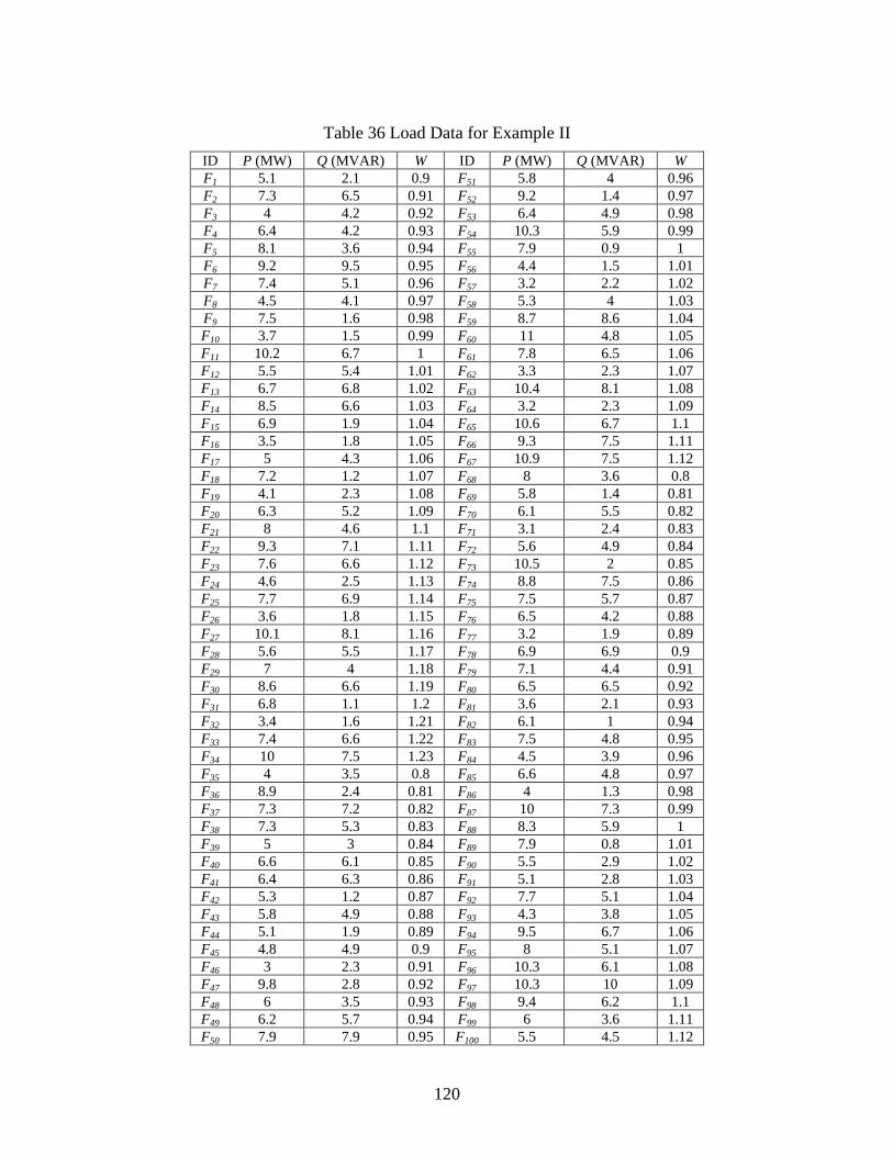
120

Table 36 Load Data for Example II ID P (MW) Q (MVAR) W ID P (MW) Q (MVAR) W F1 5.1 2.1 0.9 F51 5.8 4 0.96 F2 7.3 6.5 0.91 F52 9.2 1.4 0.97 F3 4 4.2 0.92 F53 6.4 4.9 0.98 F4 6.4 4.2 0.93 F54 10.3 5.9 0.99 F5 8.1 3.6 0.94 F55 7.9 0.9 1 F6 9.2 9.5 0.95 F56 4.4 1.5 1.01 F7 7.4 5.1 0.96 F57 3.2 2.2 1.02 F8 4.5 4.1 0.97 F58 5.3 4 1.03 F9 7.5 1.6 0.98 F59 8.7 8.6 1.04 F10 3.7 1.5 0.99 F60 11 4.8 1.05 F11 10.2 6.7 1 F61 7.8 6.5 1.06 F12 5.5 5.4 1.01 F62 3.3 2.3 1.07 F13 6.7 6.8 1.02 F63 10.4 8.1 1.08 F14 8.5 6.6 1.03 F64 3.2 2.3 1.09 F15 6.9 1.9 1.04 F65 10.6 6.7 1.1 F16 3.5 1.8 1.05 F66 9.3 7.5 1.11 F17 5 4.3 1.06 F67 10.9 7.5 1.12 F18 7.2 1.2 1.07 F68 8 3.6 0.8 F19 4.1 2.3 1.08 F69 5.8 1.4 0.81 F20 6.3 5.2 1.09 F70 6.1 5.5 0.82 F21 8 4.6 1.1 F71 3.1 2.4 0.83 F22 9.3 7.1 1.11 F72 5.6 4.9 0.84 F23 7.6 6.6 1.12 F73 10.5 2 0.85 F24 4.6 2.5 1.13 F74 8.8 7.5 0.86 F25 7.7 6.9 1.14 F75 7.5 5.7 0.87 F26 3.6 1.8 1.15 F76 6.5 4.2 0.88 F27 10.1 8.1 1.16 F77 3.2 1.9 0.89 F28 5.6 5.5 1.17 F78 6.9 6.9 0.9 F29 7 4 1.18 F79 7.1 4.4 0.91 F30 8.6 6.6 1.19 F80 6.5 6.5 0.92 F31 6.8 1.1 1.2 F81 3.6 2.1 0.93 F32 3.4 1.6 1.21 F82 6.1 1 0.94 F33 7.4 6.6 1.22 F83 7.5 4.8 0.95 F34 10 7.5 1.23 F84 4.5 3.9 0.96 F35 4 3.5 0.8 F85 6.6 4.8 0.97 F36 8.9 2.4 0.81 F86 4 1.3 0.98 F37 7.3 7.2 0.82 F87 10 7.3 0.99 F38 7.3 5.3 0.83 F88 8.3 5.9 1 F39 5 3 0.84 F89 7.9 0.8 1.01 F40 6.6 6.1 0.85 F90 5.5 2.9 1.02 F41 6.4 6.3 0.86 F91 5.1 2.8 1.03 F42 5.3 1.2 0.87 F92 7.7 5.1 1.04 F43 5.8 4.9 0.88 F93 4.3 3.8 1.05 F44 5.1 1.9 0.89 F94 9.5 6.7 1.06 F45 4.8 4.9 0.9 F95 8 5.1 1.07 F46 3 2.3 0.91 F96 10.3 6.1 1.08 F47 9.8 2.8 0.92 F97 10.3 10 1.09 F48 6 3.5 0.93 F98 9.4 6.2 1.1 F49 6.2 5.7 0.94 F99 6 3.6 1.11 F50 7.9 7.9 0.95 F100 5.5 4.5 1.12

121

Table 37 and Table 38 show the expected available generation data. The generation restoration time is the time at which the indicated generation becomes available at distribution system substations.

Table 37 Generation Data for Example I

P (MW) Q (MVAR) T0 0 0 T1 5 3.10 T2 7.5 4.65 T3 9 5.58 T4 10 6.20 T5 13 8.05 T6 20 12.40 T7 25 15.49 T8 37 22.93

Table 38 Generation Data for Example II

P (MW) Q (MVAR) T0 0 0 T1 4 2.5 T2 12 7.4 T3 28 17.4 T4 48 29.7 T5 84 52.1 T6 100 62.0 T7 120 74.4 T8 124 76.8 T9 128 79.3 T10 140 86.8 T11 160 99.2 T12 200 124.0 T13 228 141.3 T14 240 148.7 T15 260 161.1 T16 284 176.0 T17 292 181.0 T18 296 183.4 T19 308 190.9 T20 316 195.8

Table 39 shows the correspondences between substations and feeders in the 100 feeder system.

122

Table 39 Substation Definition

Substation Feeder 1 1 ~ 10 2 11 ~ 20 3 21 ~ 30 4 31 ~ 40 5 41 ~ 50 6 51 ~ 60 7 61 ~ 70 8 71 ~ 80 9 81 ~ 90 10 91 ~ 95, 97, 98, 100 11 96, 99

3.5.3 Illustrative Distribution Restoration Examples

3.5.3.1 Example I: Four Feeder System Example I develops the complete restoration plan for a four feeder area by using Lagrangian relaxation with subgradient iterations. The number of time intervals selected was 8, all with the same time value. Note that the estimated time horizon of the restoration process is obtained by determining, from the available generation, the time when the total load is expected to be restored.

Solution to the four feeder example using the proposed LR algorithm is shown in Table 40. Feeder status transitions (change in restoration index sign) take place at T1, T3, T6 and T7. Note that at the restoration index zero crossing, due to the proximity between OFF status and ON status, additional considerations (e.g., operator permissive action) may be needed to determine the appropriate restoration instant. As an example, due to the discrete nature of the problem, it may be desired to delay the restoration of a particular feeder. This operator discretion (OD) status is shown in Table 40.

Table 40 Restoration Plan for Example I Dual Solution

F1 F2 F3 F4 T1 Off Off On Off T2 Off Off On Off T3 Off Off On OD T4 Off Off On OD T5 Off Off On On T6 On Off On On T7 On OD On On T8 On On On On OD = OPERATOR DISCRETION

123

Table 41 shows the restoration index for each time interval of Example I. The restoration index varies with time reflecting the feeder restoration status. This index may be used instead of the corresponding restoration plan (Table 40) during restoration. For example, visualization of the restoration process can be developed from the restoration index of each feeder. This may be useful to the operator in the decision making as operator situational awareness is often improved by a visual representation of calculated strategies. This point is discussed further below.

Table 41 Restoration Index for Example I Positive Values are Associated with On Status

Negative Values are Associated with Off Status

F1 F2 F3 F4 T1 -0.55 -1.44 0.73 -9.9e-14 T2 -0.19 -2.00 1.61 -8.9e-16 T3 -0.19 -2.00 1.61 8.9e-15 T4 -0.19 -2.00 1.61 4.0e-14 T5 -8.9e-15 -1.64 1.71 0.28 T6 0.84 -5.3e-15 2.13 1.52 T7 0.84 1.7e-15 2.13 1.52 T8 4.59 7.30 4.00 7.04

Figure 64 illustrates the concept of visualization. In Example I, the evolution of the restoration index of each feeder is rendered in a visual format for the eight time intervals. Light colors indicate feeders recommended for restoration while dark colors indicate feeders that are not recommended. Note that the intensity of the shading is indicative of the restoration index value.

Figure 64 Suggested Restoration Plan through Visualization

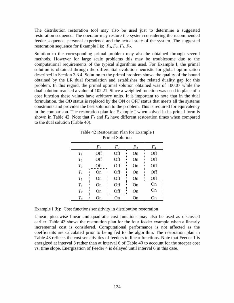
124

The distribution restoration tool may also be used just to determine a suggested restoration sequence. The operator may restore the system considering the recommended feeder sequence, personal experience and the actual state of the system. The suggested restoration sequence for Example I is: F3, F4, F1, F2.

Solution to the corresponding primal problem may also be obtained through several methods. However for large scale problems this may be troublesome due to the computational requirements of the typical algorithms used. For Example I, the primal solution is obtained through the differential evolution heuristic for global optimization described in Section 3.3.4. Solution to the primal problem shows the quality of the bound obtained by the LR dual formulation and establishes the related duality gap for this problem. In this regard, the primal optimal solution obtained was of 100.07 while the dual solution reached a value of 102.21. Since a weighted function was used in place of a cost function these values have arbitrary units. It is important to note that in the dual formulation, the OD status is replaced by the ON or OFF status that meets all the systems constraints and provides the best solution to the problem. This is required for equivalency in the comparison. The restoration plan for Example I when solved in its primal form is shown in Table 42. Note that F1 and F4 have different restoration times when compared to the dual solution (Table 40).

Table 42 Restoration Plan for Example I Primal Solution

F1 F2 F3 F4 T1 Off Off On Off T2 Off Off On Off T3 Off Off On Off T4 On Off On Off T5 On Off On Off T6 On Off On On T7 On Off On On

T8 On On On On

Example I (b)

Linear, piecewise linear and quadratic cost functions may also be used as discussed earlier.

: Cost functions sensitivity in distribution restoration

Table 43 shows the restoration plan for the four feeder example when a linearly incremental cost is considered. Computational performance is not affected as the coefficients are calculated prior to being fed to the algorithm. The restoration plan in Table 43 reflects the cost sensitivities of feeders to linear functions. Note that Feeder 1 is energized at interval 3 rather than at interval 6 of Table 40 to account for the steeper cost vs. time slope. Energization of Feeder 4 is delayed until interval 6 in this case.

125

Table 43 Restoration Plan for Four Feeder System Linear Cost Functions

F1 F2 F3 F4 T1 Off Off On Off T2 Off Off On Off T3 On Off On Off T4 On Off On Off T5 On Off On Off T6 On Off On On T7 On On On On T8 On On On On

Example I (c)

Cold load pickup considerations are also very important during restoration. For Example I, Feeder 3 shows an adverse condition that increases its reactive power demand to 4.9 MVAR (from 1.9 MVAR). This demand requires 2 time intervals before reducing back to the estimated steady state value of 1.9 MVAR. For purposes of this development, the 4.9 MVAR condition is left for the 2 time intervals as shown in

: Cold load pickup

Figure 53. This modifies the restoration plan by energizing Feeder 3 at T3 rather than at T1 as shown in Table 40. For the first two time intervals, energizing Feeder 3 has an operator discretion status. The full restoration plan for the CLPU variation is shown in Table 44.

Solution to the cold load pickup variation was very difficult to solve using the subgradient iteration method even for the four feeder case study. However, the proposed model shown in Section 3.2.4.4 may be applied in LR by replacing the algorithm used to solve the outer problem. In this regard, solution to the previous example was found to have better convergence characteristics by using the differential evolution heuristic explained in Section 3.3.4 rather than the subgradient iterations approach. As a tradeoff, this heuristic is potentially slower as it does a randomly guided search of the solution space. In addition, the probabilistic nature of the algorithm does not guarantee that the best solution (or the same solution) will be found every time. Convergence of the heuristic generally takes place in around 600 iterations. Out of 10 independent runs the algorithm reached the best solution found (shown in Table 44) four times while obtaining two other bounds in the other runs.

Table 44 Restoration Plan for Four Feeder System Cold Load Pickup

F1 F2 F3 F4 T1 Off Off OD Off T2 Off Off OD Off T3 Off Off On Off T4 Off Off On OD T5 Off Off On On T6 On Off On On T7 On Off On On T8 On On On On

126

3.5.3.2 Example II: One Hundred Feeder System The Lagrangian relaxation restoration algorithm was also tested on a 100 feeder system with 20 equally spaced time intervals for a total of 2000 decision variables. Since the total available generation is less than the total amount of estimated load, the algorithm is required to select which feeders to energize as well as the proper time interval for this action. Only fixed cost functions are considered in this example. One point to be made relating to this LR problem formulation and solution is that the solution speed is fast and can accommodate high dimension of decision variables without excessive storage.

In Example II, 44 out of the 100 available feeders were selected for restoration. The restoration plan for Example II is shown in Figure 65. The feeders omitted from the figure are those that are not restored in that time horizon.

3.5.3.3 Example III: One Hundred Feeder System - BIP In the following two examples, the number of crews constraints is set to 20 for each time interval; the number of feeder operations in the same substation is set to 10; and the specified load restoration requires load 57 to be restored no later than time interval 15, load 66 to be restored no later than time interval 12, and load 97 to be restored no later than time interval 15.

Example III (a)

In order to test the effects of moving time horizon Ntf on computation speed and objective function values, the BIP based optimal distribution restoration problem is tested under different moving time horizon values. The simulation results are given in

: Maximize the total restored weighted energy

Table 45.

Table 45 Simulation Results under Different Ntf

Ntf Obj. Value (Maximization)

Actual Restored system load

Number of Resotered Feeders (Loads)

Computation Speed

1 3729.134 46.498% 48 0.191 sec 2 3748.133 46.454% 46 1.766 sec 3 3748.441 46.469% 47 25.089 sec 4 3746.862 46.498% 47 4 min 21 sec 5 3748.177 46.410% 45 20 min 36 sec

From this table, it shows that the computation time increases with the increase of Ntf but the optimal solution does not necessarily increase by increasing Ntf. This is because the absolute or relative optimality tolerance gap has been reached for the optimal solution. For this example, from both the objective function and computation time point of view, the best time horizon was two steps.

The simulation results are also compared with LR-subgradient based restoration algorithm. Table 46 shows the simulation results from LR-subgradient based restoration algorithm.

127

Table 46 Simulation Results from LR-Subgradient Algorithm

Objective value (Maximization)

Number of Resotered Feeders (Loads)

Computation Speed

3626.3 43 Around 23 sec

Comparing the simulation results in Table 46 with the simulation results in Table 45 when Ntf=2, we can see that from the number of restored feeders and objective value point of view, the BIP based optimal distribution algorithm has better performance than the LR-subgradient based optimal restoration algorithm. The computational speed appears comparable between the two approaches but the systems were not tested on identical computers.

Example III (b)

In order to test the algorithm efficiency under different circumstances, the BIP based optimal distribution restoration problem is tested under different system load percentage. The simulation results are given in

: Restore k% system load in the shortest time

Table 47.

Table 47 Simulation Results under Different System Load Percentage k%

Restore k% System load

in the shortest

time

First time interval restoring k% system load

Actual Restored

system load

Restored Weighted Energy

(Maximization)

Number of Restored Feeders (Loads)

Computation Time (sec)

k% = 100% N/A 46.38% 3285.919 58 25.883 k% = 90% N/A 46.38% 3286.615 58 18.588 k% = 80% N/A 46.38% 3279.339 58 49.918 k% = 70% N/A 46.38% 3288.731 58 14.301 k% = 60% N/A 46.263% 3282.089 58 25.928 k% = 50% N/A 46.263% 3283.022 58 19.662 k% = 40% 16 46.277% 3271.401 58 0.149 k% = 30% 13 46.277% 3271.401 58 0.153 k% = 20% 10 46.277% 3271.401 58 0.162 k% = 10% 5 46.277% 3269.945 58 0.238

From this table we can see that when the system generation capacity is sufficient, the first time interval restoring k% system load can be found quickly and the computation speed is much faster than the case when system generation capacity is not enough to restore k% system load.

3.5.4 Additional Computational Results and Observations The Lagrangian relaxation algorithm discussed in this thesis shows a nearly linear execution time as the problem dimension increases. Figure 66 shows the algorithm execution time plotted against the number of variables. A trend line shows the expected computation time based on a linear estimation.

128

Control parameters play an important role in algorithm convergence. There are three main control parameters in the subgradient iterations approach: step length μ, convergence factor α and maximum iterations without improvement iter. The algorithm had good convergence characteristics with μ and α set to the typical values of 2.0 and 0.5 respectively. For the examples under consideration, a value of iter of 500 showed good convergence characteristics. Examples I and II discussed in this research use these values of μ, α and iter as control parameters.

129

Figure 65 Graphic Representation of the Restoration Plan for Example II.

130

1000 1200 1400 1600 1800 2000 2200 2400 2600 2800 3000 10

15

20

25

30

35

40

45

Number of variables

Experimental Values Trend Line

Feeders: 75 Intervals: 15






Exec

utio

n tim

e (s

)

Figure 66 Computational Time as a Function of the Number of Variables for a

Subgradient Based LR Solution

In the event of no convergence, the value of iter may be increased to allow more evaluations with the same step length to be performed. A small value of iter (e.g. 10, 20, 50) speeds up convergence but is more susceptible to not obtain any solution as the step length quickly approaches zero. A larger value of iter (e.g. 1000, 2000) is more likely to obtain a solution although convergence is only guaranteed when the number of iterations (iter) tends to infinity which is not practical. Convergence characteristics of the subgradient iterations method are discussed in further in [96], [99] and [108].

3.5.5 Summary of Examples The previous examples show the applicability of the Lagrangian relaxation algorithm and Binary Integer Programming algorithm to the distribution systems restoration problem. The restoration plans developed here optimize the system by minimizing the outage cost, maximizing restored weighted energy, and minimizing the time to restore k% system load. Critical loads in the system are taken into account through cost sensitivities and other characteristics such as cold load pickup. Solution of the CLPU modeling is difficult by using the faster subgradient iterations method, however, heuristics show that it may be possible to obtain a good bound to this problem using the LR dual formulation.

Application of the problem to a larger test system is also shown. This system is of 2000 variables and its solution was obtained in the operational real time frame suggested. Solution of a 3000 system was also obtained and its execution time is shown in Figure 66. It is important to note, that the algorithm is performed in Matlab which is generally a slower programming language. Execution time for data processing, that is, time to obtain expected generation curve, load information and other estimations is not accounted for.

131

3.6 Conclusions, Recommendations and Future Work

3.6.1 Conclusions This work provides an alternative procedure for developing a step-by-step restoration plan for radial distribution systems after a blackout. The suggested approaches use a Lagrangian relaxation algorithm and a Binary Integer Programming algorithm to determine the optimal restoration feeder sequence for the distribution system. These optimal restoration plans are performed by minimizing the system outage cost, maximizing system total weighted energy, and minimizing time spent to restore k% system load. A subgradient method used to calculate λ in the LR formulation is found to render the approach suitable for large problems. A moving time horizon method is introduced to coordinate the computation efficiency and optimal solutions. The restoration algorithms are intended to assist the operator during restoration, by determining the order and time in which feeders should be energized. A restoration index and a visualization approach for restoration are also shown. The restoration index may be very useful in restoring the system as it gives a rapid indication of the feeder status during restoration. The subgradient based LR solution and BIP with a suitable moving time horizon algorithm of the distribution restoration problem are found to have favorably fast computation speed and low storage requirements. In contrast, the subgradient may present convergence problems in some cases.

The algorithm was tested on several test beds with a 4-feeder test system and a 100-feeder test system being discussed. The 4-feeder system provides a simple example suitable for showing the main remarks of the method and its solution. The 100 feeder extends the discussion to a larger system. This 100 feeder test system is similar to those that are being targeted in this work. The restoration plans for these examples are developed considering a minimum outage cost objective and a minimum restoration time for k% system load restoration. Other objectives that consider a weighted priority ranking or system security may also be adopted by replacing the cost function with the pertinent model.

The results show the applicability of the proposed algorithms in the restoration problem under consideration. The algorithms successfully obtain the optimal restoration sequence for the systems under study guided by the several objectives and the algorithm inputs. Due to the dual characteristics of the LR method, global convergence is not guaranteed as some constraints may be ignored during the optimization problem. In addition, the total accuracy of the solution will also depend on the estimates used for load and expected available generation. The algorithm represents an effort to reduce the burden operators have during the restoration process by providing customized plans for specific conditions. This form of automated (or alternatively semi-automation) tool is expected to run in parallel with the restoration process with each run using updated values for loads and expected generation providing a better estimation.


• Novel approaches for determining proper strategies for restoration of the distribution system.

132

• Formulation of the distribution restoration problem as the dual of the unit commitment problem.

• Formulation of the distribution as a binary-integer programming problem with two different objectives and expanded practical constraints.

• Modeling of the distribution restoration problem and related phenomena such as cold load pickup.

• Restoration infrastructure and suggested implementation of the proposed operator-permissive tool.

3.6.2 Future Work The work previously presented shows an alternative approach to the distribution system restoration problem. It mainly focuses in the decision-making process of the load restoration stage and addresses a common concern of operators. This problem was solved using the Lagrangian relaxation method and BIP method. Several questions should be addressed in the future in relation to the work presented in this thesis. These lines of future work can be classified within two main groups: Improvements to the distribution system restoration problem formulation and improvements to the solution method.

Future work related to the distribution system restoration problem should enhance the models used within the problem in order to obtain a better restoration plan. Some alternatives to future work within this group include:

• Further modeling of the CLPU phenomena

• Evaluation of the impact of phase sequence in capacitor switching

• Evaluation of the effect of system transmission and system voltage profile constraints in the distribution system restoration problem

• Determine the role and candidacy of this tool as part of the modern grid initiatives recently being suggested

• Additional system configurations

• Additional system constraints.

Improvements to the solution method should aim at solving systems of a larger scale and more complex in nature while retaining the accuracy of the solution. As lines of future work within the solution method can be mentioned:

• Convergence studies for common distribution system restoration examples.

• Hybrid formulations and other state of the art algorithms that improve performance of the algorithm without major loss of accuracy.

3.6.2.1 Networked Systems A future work topic within this subject is the consideration of networked systems. Networked systems add the complexity that distribution loads may be energized from several paths. Even in the case of systems that are mainly radial, but contain transfer

133

switches, the analysis and modeling methods required are different from that shown in this thesis (see Figure 67 for example). In addition, several constraints that incorporate all the possible paths and the utility considerations when operating distribution systems may be required in order to account for the different system topologies.

Figure 67 Example of Networked System with Transfer Switches

A potential alternative for the analysis of this problem is through the use of the incidence matrix [46]. The use of the incidence matrix provides a general description of the system by showing, in a similar way to the admittance matrix, how buses are connected. Through the use of some of the Boolean properties of the incidence matrix, the configuration that leads to a fully restored system may be obtained. This may be coupled with the method proposed in this thesis in either a sequential or simultaneous arrangement to obtain the optimal sequence for restoration.

Some of the unknowns to the analysis of the networked problem include:

• Problem dimension and execution time for heavily networked systems

• Assessing system reconfiguration

• Type and how to include the constraints

• Modeling requirements

• The implementation infrastructure required for networked systems.

134

Part IV. Automated Optimal Transmission System

Restoration

135

4.1 Introduction

4.1.1 Background Restructuring of the electric power industry unbundled the originally integrated and centralized industry: the electric power generation, transmission and distribution no longer reside in a same utility [109]. These functions are now performed by independent generation companies, transmission companies, and distribution companies. The advent of competitive electricity markets stimulates more frequent electric power transactions along the transmission networks. This causes bulk power systems to operate close to their design limits, and hence makes the power systems more vulnerable to potential blackouts. All these changes pose more challenges to an already complex problem – power system restoration.

Power system restoration following a blackout, complete or partial, is one of the most important tasks for power system operators in the control center. Restoring the power system to normal operation is a centralized complex process: the internal integration of electric power system requires an integrated restoration process to coordinate the restoration of different sub-systems: generation, transmission, and distribution; the non-integrated and decentralized industry structure after liberalization makes the coordination harder. The process must observe component constraints and power system steady-state and stability constraints [1-2]. Most power systems rely on off-line restoration plans that are developed for selected scenarios of contingencies, equipment outages, and the available resources. Since the actual scenario is hard to predict in the planning stage, the restoration plan can only serve as a guide for real-time on-line restoration. Dispatchers need to be aware of the system real-time operation conditions, so that they can adapt to the changing system conditions during restoration process.

A practical strategy to facilitate automated system restoration is to develop an individual module for generation system, transmission system and distribution system. These modules are then linked and coordinated through the strategy module to provide best strategy procedure for the restoration of power systems, as shown in Figure 68. The transmission system restoration after a blackout is a critical process for a quick and safe system restoration: it builds up the skeleton to facilitate the restoration of generation and distribution system. However, it is a complex combinatorial problem to maximize the restored transmission lines by observing all system constraints, static or dynamic. In this section, an MILP-based computational tool is proposed that can be used to provide guidance to the dispatchers in the operational environment so that transmission system restoration can adapt to the changing system conditions.

136

Figure 68 Power System Restoration Strategy

4.1.2 Report Organization The report is organized into four sections. Section 1 introduces the project background. Section 2 presents MILP-based optimal transmission system restoration. Section 3 describes the illustrative examples and results of applying the developed methodology developed for a 6 bus test system. Section 4 concludes the optimal transmission restoration from application of the proposed methodology.

Power System Restoration

Generation System

Transmission System

Distribution System

Customer/ Load

Strategy Module

Generation Capability

Optimization

Transmission Path Search

Constraint Checking

Distribution Restoration

137

4.2 Optimal Transmission System Restoration

4.2.1 Review Transmission system restoration is a critical part of the integrated power system restoration process. It builds the skeleton to facilitate the restoration of generation and the distribution system: generation units rely on this skeleton to pick up appropriate amount of loads to maintain a viable balance during restoration and distribution substations rely on this skeleton to restore lost loads. The corresponding optimization problem is of combinatorial nature.

Transmission system restoration involves time-consuming switching operations to energize tripped high voltage transmission lines. Overvoltage is a major concern during energization of high voltage transmission lines [31, 110]. Energizing unloaded transmission lines, especially long EHV transmission lines, or underground cables (oil-filled or high pressure pipe) will incur sustained power frequency over-voltages. Sustained overvoltage may over-excite transformers, generating harmonic distortions and overheating, and may cause generator under-excitation, or even self-excitation and instability. The operation of breakers will incur switching transients. Switching transients on long HV lines, although of short duration, may cause arrestor failures, particularly if coupled with sustained overvoltage conditions. Energizing transmission lines may also cause harmonic resonance. Harmonic resonance on lightly loaded lines may result in very high voltage that may be amplified by transformer over-excitation [35]. In any event, during the transmission system restoration, the reactive absorption (under-excitation) capability of generator units in the system is of considerable importance to maintain a safe and stable transmission line re-energization. Systematic procedures dealing with the control of sustained overvoltage by means of optimal power flow programs can be found in [111-114]. Methods that deal with harmonic overvoltage are discussed in [114-117]. Some simple and approximate methods to deal with the evaluation of transient and sustained overvoltage and asymmetry issues for transmission line energization can be found in [118-119]. A discussion about preparation of the network for re-energization and energization of HV transmission lines can be found in [30-31, 120], and the special treatment of restoring underground cables is discussed in [63]. For EHV transmission lines, there are often shunt reactors connecting the end buses. During the transmission restoration process, the restored system is often lightly loaded. Under this circumstance, the EHV capacitor line charging is much greater than the normal or heavy load operation conditions, and hence incurs sustained overvoltage. The shunt reactors can be used for overvoltage control through counter-balancing the EHV lines’ capacitor line charging [113-114, 120, 121-123]. Another important issue during the transmission restoration process is the lead and lag reactive power capability limits of synchronous machines in the restored system. These limits are important to maintain system voltage under allowed span for high charging current requirements of lightly loaded transmission lines, or for the high reactive currents drawn by the start-up of power plant auxiliary motors [68, 72, 110, 124-125].

138

Transmission system restoration is of a mixed variable nature: the status of transmission lines is binary, and the phase angle, voltage magnitude, transmission line flow, generation output and load are real numbers. The restoration of transmission lines can be formulated as optimization problems with different objectives subject to system constraints. In order to develop better restoration strategies, researchers have investigated various approaches. Expert systems [113, 126, 143] were applied to develop restoration strategies through integrating operators’ knowledge and experience and transferring them into heuristic rules. Intelligent algorithms such as Artificial Neural Networks (ANN) [21], Fuzzy logic [115], and Genetic Algorithm (GA) [144-145] are also used to solve this problem. Pertri Nets (PNs) are also used to model the power system restoration process [20, 146-147]. Some researchers also investigated modeling the transmission restoration process as optimization problems, including: mathematical programming [24, 135], Mixed-Integer Programming (MIP) [148], and Discrete Particle Swarm Optimization (DPSO) [149].

4.2.2 MILP Based Optimal Transmission System Restoration Transmission System Restoration (TSR) is of a mixed nature: the status of transmission line is a binary variable, with 1 representing “Closed” and 0 representing “Open”; the other variables, such as voltage magnitude, phase angle, generation output, load level, and line flow, are continuous real numbers. The objective of TSR is to recover a skeletal network and provide enough transmission capacity for next stage’s load recovery. Based on the Mixed Integer Linear Programming (MILP) algorithm, a methodology is proposed to develop optimal TSR strategies.

4.2.2.1 Modeling Optimal Transmission Path Search as an MIQCP Problem In order to meet the objective of TSR, the transmission path search is modeled as an optimization problem. The objective is to restore as many transmission lines as possible during the restoration process. By restoring as many transmission lines as possible, this will energize a skeletal transmission path and prepare for the next stage of power system restoration – restoring distribution system feeders. At this stage of TSR, it is assumed there is a series of time intervals and during each time interval the available generation output is known (from the generation restoration plan). The objective function is to maximize the total number of transmission lines energized and at the same time look NT time intervals into future. Consider

( )1 1

T LN Nt t

tmax Lω

= =

⋅∑∑

90

In the optimal transmission path search problem, at each time interval, the following variables are known:

• Shunt reactor capacity and location

• Generator reactive power lower/upper limits

• Active load lower/upper limits

• Reactive load lower/upper limits

139

• Line reactive power charging

• Maximum number of operation limits.

While conversely, the following variables are unknown:

• Generator active power output

• Generator reactive power output

• Bus voltage magnitude and phase angle

• Transmission line status

• Active load values

• Reactive load values

• Line flow values

The constraints should include:

• Voltage limits

• Line flow limits

• Generator real and reactive limits

• Loads

• Switching constraints – single line or other switching transient considerations

• Frequency variation limits

Among these constraints voltage limits are the most critical during TSR since most loads are not restored and the objective is to recover a skeletal network and provide enough transmission capacity for next stage's load recovery. In this situation, the overvoltage caused by lighted loaded EHV/HV transmission line's charging current is a primary concern while line flow limits (mainly active power) are generally not a problem.

For the EHV transmission lines (500KV and above), there are often reactors that are designed to balance the line charging. So during the TSR whenever an EHV line is switched ON, the reactors at the ending side of this line are switched ON with the line to counter-balance the line reactive power charging. Generator reactive power output is adjusted (typically underexcited) to maintain bus voltages between lower and upper limits.

Specifically, the optimal transmission path search can be formulated as follows:

( ) ( )1 1 1

NN N iT Lt t t t

i it= = i=

maxωLωP

+

∑ ∑ ∑

91

140

( )

( )

, , ,1

, , , ,1

. .

power flow equations :m

t t t t t t tg i load i i j ij ij i j ij

j

mt t t t t t t

g i load i reactor i i j ij ij i j ijj

s t

P P V V y L cos

Q Q Q V V y L sin

δ δ θ

δ δ θ

=

=

= + − −

= + + − −

∑

∑

( ) ( )( ) ( )

, , ,

, , ,

Line flow limits: t t t t t t t maxij ij ij i ij i j i j ij ij

t t t t t t t maxij ij ij i ij i j i j ij ij

P y L V cos V V cos P

Q y L V sin V V sin Q

θ δ δ θ

θ δ δ θ

= − − − ≤ = − − − − ≤

Voltage magnitude limits:

Voltage phase angle limits:

min t maxi i imin t max min t t max

i i i ij i j ij

V V Vδ δ δ δ δ δ δ

≤ ≤

≤ ≤ , ∆ ≤ − ≤ ∆

, , ,

, , ,

Gen. active power limits:

Gen. reactive power limits:

min t maxg i g i g i

min t maxg i g i g i

P P P

Q Q Q

≤ ≤

≤ ≤

, , ,

, , ,

Active load limits:

Reactive load limits:

min t maxload i load i load i

min t maxload i load i load i

P P P

Q Q Q

≤ ≤

≤ ≤

{ }1Single line switching constraint: , 0,1t t tL L L− ≤ ∈

( )1

1Max # of line switching constraint :

LNt t t

SL L N−

=

− ≤∑

The power flow constraints can be modeled as nearly linear at this stage and voltage constraints can be modeled as linear or quadratic functions. A simplified formulation is listed below:

( ) ( )1 1 1

NN N iT Lt t t t

i it= = i=

maxωLωP

+

∑ ∑ ∑

92

( )

( ) ( )

, ,, ,

1 1

, , , , ,1 1

. .

Gen. reactive power constraint : , 0

Active power constraint(KCL) :

g L

t fi i

N Nt min t ch re t min

g i g ii

N Nt t t t t t

g i ki ki i ij iji i

s t

Q L Q Q Q

P P L P P L

= =

= =

≥ − ∀ ≤

+ ⋅ = + ⋅

∑ ∑

∑ ∑

( ) ( ), , , , , , ,1 1

Reactive power constraint(KCL) : ( )t f

i iN Nt t ch t t t

g i ki ki ki re i ij iji i

Q Q Q L Q Q L= =

+ + ⋅ = + ⋅∑ ∑

, ,, , ,Gen. active power limits : t min t t max

g i g i g iP P P ≤ ≤

, ,, , ,Gen. reactive power limits : t min t t max

g i g i g iQ Q Q ≤ ≤

141

, ,Active load limits : t min t t maxi i iP P P ≤ ≤

, ,Reactive load limits : t min t t maxi i iQ Q Q ≤ ≤

Active line flow limits : min t maxP P P ≤ ≤

{ }

( )

1

1

1

Reactive line flow limits :

Single line switching constraint : , 0,1 , ,

Max # of line switching constraint :L

min t max

t t t

Nt t t

S

Q Q QL L L t

L L N

−

−

=

≤ ≤

≤ ∈ ∀ ∀

− ≤∑

The unknown variables in this formulation are:

Line status: tL

Generator active/reactive power: tigP , / ,

tg iQ

Active/reactive load: tiP / t

iQ

Line active/reactive flow: tP /

tQ

There are multiplication terms between the unknown variables line status and line flow. So this formulation is a Mixed-Integer Quadratic Constrained Programming (MIQCP). In this MIQCP formulation (3), the system is assumed to be lossless. Under this assumption, the calculated total active load should be greater than the total active generation at time t. Also, the line charging is assumed to be at the no-load value. In the following iterative optimal TSR, the solution feasibility will be checked with a constraint checking module, as with appropriate power system tools and then adjust the line ON/OFF status accordingly. If there is any violation, the corresponding line switch that causes this violation will be blocked. Generators are assumed to operate under power factor control rather than using AVRs to maintain specific terminal voltages.

4.2.2.2 Linearizing the Pseudo-quadratic Term In the equation set (3), the product between unknown variables line status and line flow brings quadratic constraints to the problem. Still, it is known that the line status

tL takes two possible values: 0 or 1. Thus, the multiplication of line flow tP / tQ with this binary

variable can only be 0 or tP /

tQ and this quadratic term is only a “Pseudo-quadratic”. These Pseudo-quadratic terms can be converted into linear ones. For the purpose of simple expression and easy to follow, equation (4) is used to represent the pseudo-quadratic term that is a multiplication between a binary variable and a real variable. And ℜ represents the real space.

{ }1 1 1 1, 0,1 ,x p x p∈ ∈ℜ 93

142

Two new variables: M and 3x are introduced to help linearize equation (4). Define M as an arbitrarily large positive number, M +∈ℜ ( +ℜ represents positive real space), if

1maxp and 1

maxp +∈ℜ are known, then 1maxM p= . Now define 3 1 1 3,x x p x= ∈ℜ to represent

the multiplication term 1 1x p . Then Equation 93 can be converted to this system of linear constraints:

3 1

3 1

3 1 1

3 1 1

1

(1 )(1 )

x Mxx Mx

x p M xx p M x

p M

≤− ≤ ≤ + −− ≤ − + − ≤

94

Notice that the last constraint 1p M≤ comes from the assumption on M and the reality that variable 1p is always a limited real number in our problem. This constraint helps formulate a simpler feasible region and hence improve computation efficiency. The equivalence between Equation 93and Equation set 94 is proved as following:

♦ Proof: It does not need to consider the constraint 1p M≤ in the proof since this is the assumption for the definition of M. 3 1 1x x p= will be proved based on the following conditions:

1. { }1 10,1 ,x p∈ ∈ℜ 2. M is an arbitrarily large positive number, M +∈ℜ 3. Constraint set 94.

If 1 1x = , Equation 94 is equivalent to Equation 95:

3

3

3 1

3 1

x Mx M

x px p

≤− ≤ ≤− ≤ −

95

Because M is an arbitrarily large positive number, the first two inequality constraints in Equation 95 always hold. So Equation 95 can be simplified to be:

3 1

3 1

x px p≤

− ≤ − 96

Obviously, Equation 96 is equivalent to:

3 1x p= 97

143

If 01 =x , Equation 94 is equivalent to:

3

3

3 1

3 1

00

xx

x p Mx p M

≤− ≤ ≤ +− ≤ − +

98

Because M is an arbitrarily large positive number, the last two inequality constraints in Equation 98 always hold. So Equation 98 can be simplified to be:

3

3

00

xx≤

− ≤ 99

Obviously, Equation 99 is equivalent to:

3 0x = 100

From the above two possibilities, it is known that Equation 94 is equivalent to the following “either-or” problem:

1 1

3 1 3

1 0

0x x

either orx p x

= = = =

101

So Equation 101 includes all the possibilities as listed in Table 48 below. That is to say 3 1 1x x p= .

Table 48 Possible Values of Variables

Variable 1x 1p 3x

Values 0 1p 0 1 1p 1p

. . .Q E D

4.2.2.3 Modeling Optimal Transmission Path Search as an MILP Problem Based on the standard rule to linearize a pseudo-quadratic term which is derived in the previous, the MIQCP problem 92 can be easily converted to the MILP problem 102 .

( ) ( )1 1 1

NN N iT Lt t t tl l i i

t= l= i=maxωLωP

+

∑ ∑ ∑ 103

s.t.

Gen. reactive power constraint: ∑ ∑= =

−≥g LN

i

N

l

rel

chl

tl

tig QQLQ

1 1

min,, )(

144

Active power constraint (KCL): 0,1

2,1

1, =+−− ∑∑ tig

ti

fiN

=ii

tiN

=ii PPXX

Reactive power constraint (KCL): ire,t

iit

ig,t

kil,

tiN

=i

chkil,

fiN

=ii

tiN

=ii Q=PPFQLQ+XX ..

114,

13, −+− ∑∑∑

Additional constraints due to the X1,i - Pmax,ki .Ll,ki 0≤ simplification for X1,i = Pl,ki . Ll,ki: - X1,i - Pmax,ki.Ll,ki 0≤ X1,i - Pl,ki + Pmax,ki.Ll,ki kiPmax,≤

-X1,i+Pl,ki+Pmax,ki.Ll,ki kiPmax,≤

Additional constraints due to the X2,i - Pmax,ij .Ll,ij 0≤ simplification for X2,i = Pl, ji . Ll,ij: - X2,i - Pmax,ij.Ll,ij 0≤ X2,i - Pl,ij + Pmax,ij.Ll,ij ijPmax,≤

-X2,i+Pl,ij + Pmax,ij.Ll,ij ijPmax,≤ Additional constraints due to the X3,i - Qmax,ki .Ll,ki 0≤ simplification for X3,i = Ql,ki . Ll,ki: - X3,i - Qmax,ki.Ll,ki 0≤ X3,i - Ql,ki + Qmax,ki.Ll,ki kiQmax,≤

-X3,i+Ql,ki+Qmax,ki.Ll,ki kiQmax,≤

Additional constraints due to the X4,i - Qmax,ij .Ll,ij 0≤ simplification for X4,i = Ql,ij . Ll,ij: - X4,i - Qmax,ij.Ll,ij 0≤ X4,i - Ql,ij + Qmax,ij.Ll,ij ijQmax,≤ -X4,i+Ql,ij+Qmax,ij.Ll,ij ijQmax,≤ Gen. reactive power limits: max,min, t

ig,t

ig,t

ig, QQQ ≤≤ Gen. active power limits: max,min, t

ig,tig,

tig, PPP ≤≤

Load active power limits: max,min, t

it

it

i PPP ≤≤ Active line flow limits: maxmax

lt

ll PPP ≤≤− Reactive line flow limits: maxmax

ltll QQQ ≤≤−

X1,i = Pl,ki . Ll,ki : iii PXP max,1,max, ≤≤− X2,i = Pl, ji . Ll,ij: iii PXP max,2,max, ≤≤−

145

X3,i = Ql,ki . Ll,ki: iii QXQ max,3,max, ≤≤− X4,i = Ql,ij . Ll,ij: iii QXQ max,4,max, ≤≤−

The optimal transmission line restoration strategy for all tripped lines will be obtained by solving this MILP problem.

4.2.2.4 Formulating Optimal Transmission System Restoration Problem Based on the ideal lossless power network, the MILP based optimal transmission path search problem alone is not sufficient to produce an optimal transmission system restoration strategy that satisfies all system constraints. In order to develop a practical optimal TSR strategy, the assistance of other programs is indispensable. These programs include SCADA/EMS, EMTP, Power Flow, and the Constraint Checking Module developed in this Pserc project. The flowchart for such an iterative optimal TSR process is shown in Figure 69.

Figure 69 Iterative Optimal Transmission System Restoration

Get system variable status/values for next iteration

Read data from SCADA/EMS or other software

MIQCP Problem Formulation and Solution

Check solution feasibility with constraint checking module, EMTP, PF, etc.

Any violation? Change infeasible lines' status from

ON to OFF during this time interval.

All Line Closed or Max time interval

STOP

Y

Y

N

N

Any infeasible lines? Y

N

• Sustained power frequency overvoltage

• Switching transient

• Harmonic resonance overcoltage

• Line flow

146

4.3 Illustrative Examples

In these examples, the software tools used to solve the MILP problems are MATLAB 7.6.0 and ILOG CPLEX 11.1 under the Windows 64-bit Vista operation system. The MILP problem is formulated in MATLAB, which calls the CPLEX Mixed Integer Optimizer engine through a DLL (Dynamic Link Library) to solve the formulated problem. ILOG CPLEX Mixed Integer Optimizer includes sophisticated mixed integer preprocessing routines, cutting-plane strategies and feasibility heuristics. The default settings of MIP models are used with a general and robust branch-and-cut algorithm.

4.3.1 6-Bus Test System

4.3.1.1 System Data The 6-Bus test system includes 6 bus and 11 transmission lines. System data is provided in Table 49 - Table 51. Figure 70 One-Line Diagram of the 6-Bus Test System depicts the single-line model of the system.

Figure 70 One-Line Diagram of the 6-Bus Test System

Table 49 Generators Data Bus

Number Power Rating (MVA)

Voltage Rating (kV)

Active Power (p.u.)

Voltage Magnitude

(p.u.)

Maximum Reactive Power (p.u.)

Minimum Reactive Power (p.u.)

Maximum Voltage (p.u.)

Maximum Voltage (p.u.)

1 100 400 0.9 1.05 1.5 -0.5 1.1 0.9

2 200 400 1.4 1.05 1.5 -0.5 1.1 0.9

3 100 400 0.6 1.05 1.5 -0.5 1.1 0.9

G1

G2

G3

1

2

3

4

5

6

147

Table 50 Load Data Bus Number Power Rating

(MVA) Voltage Rating (KV) Active Power (p.u.) Reactive Power

(p.u.) 4 100 400 0.9 0.2957

5 100 400 1.0 0.3286

6 100 400 0.9 0.2957

Table 51 Branch Data Line

Number From Bus

To Bus

Power Rating (MVA)

Voltage Rating (kV)

Resistance (Ω/km) (p.u.)

Reactance (H/km) (p.u.)

Suseptance (F/km) (p.u.)

Current Limit (p.u.)

Active Power Limit (p.u.)

Reactive Power Limit (p.u.)

1 2 3 100 400 0 0.2500 0.1260 0.3082 1.5 0.75

2 3 6 100 400 0 0.1000 0.0420 1.3973 1.5 0.75

3 4 5 100 400 0 0.4000 0.1680 0.1796 1.5 0.75

4 3 5 100 400 0 0.2600 0.1050 0.6585 1.5 0.75

5 5 6 100 400 0 0.3000 0.1260 0.2000 1.5 0.75

6 2 4 100 400 0 0.1000 0.0420 1.3740 1.5 0.75

7 1 2 100 400 0 0.2000 0.0840 0.2591 1.5 0.75

8 1 4 100 400 0 0.2000 0.0840 0.9193 1.5 0.75

9 1 5 100 400 0 0.3000 0.1260 0.8478 1.5 0.75

10 2 6 100 400 0 0.2000 0.1050 0.9147 1.5 0.75

11 2 5 100 400 0 0.3000 0.0840 0.7114 1.5 0.75

4.3.1.2 Simulation Results In this simulation, it is assumed that the transmission restoration is being done in 3 steps considering the available generation units. In the first step, the generator 1 is available and two other generators are not restored yet. In the second step, generator 1 and generator 2 are available. All units are available in the last step. Simulation results for each step are described in the following. It is assumed power factor at each bus to be fixed at 0.95.

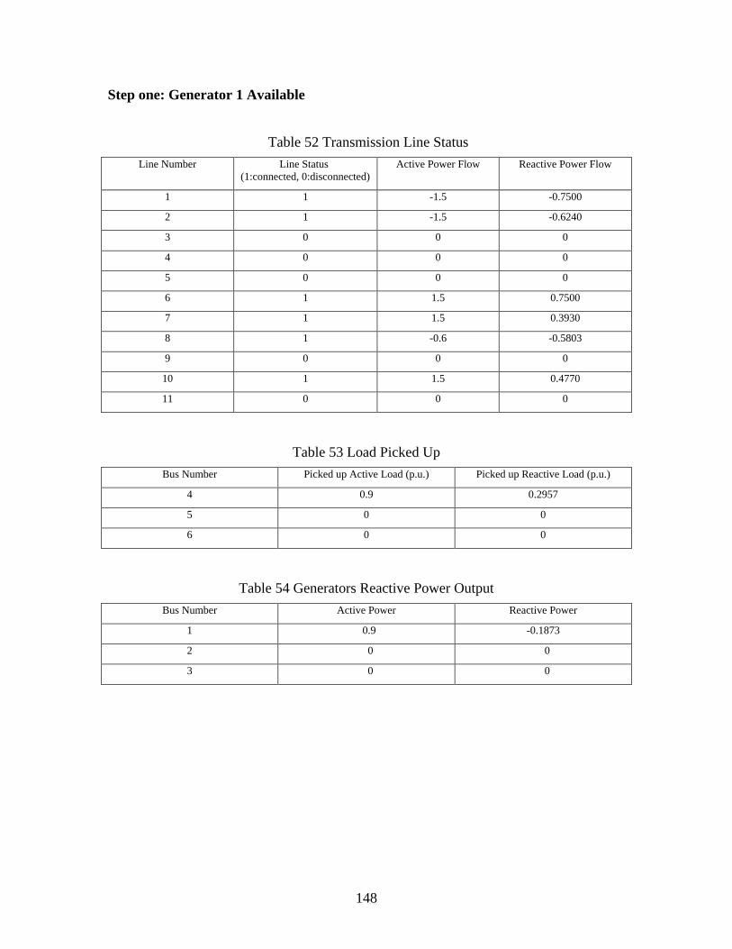
148

Step one: Generator 1 Available

Table 52 Transmission Line Status Line Number Line Status

(1:connected, 0:disconnected) Active Power Flow Reactive Power Flow

1 1 -1.5 -0.7500

2 1 -1.5 -0.6240

3 0 0 0

4 0 0 0

5 0 0 0

6 1 1.5 0.7500

7 1 1.5 0.3930

8 1 -0.6 -0.5803

9 0 0 0

10 1 1.5 0.4770

11 0 0 0

Table 53 Load Picked Up Bus Number Picked up Active Load (p.u.) Picked up Reactive Load (p.u.)

4 0.9 0.2957

5 0 0

6 0 0

Table 54 Generators Reactive Power Output Bus Number Active Power Reactive Power

1 0.9 -0.1873

2 0 0

3 0 0

149

Figure 71 System Configuration after First Step

Step 2: Generators 1 and 2 Available



1 1 1.5000 0.7500

2 1 0.9000 0.2767

3 0 0 0

4 1 0.6000 0.5993

5 1 -1.5000 -0.7500

6 1 -0.6000 0.6697

7 1 -0.5000 0.7500

8 1 1.5000 -0.5000

9 1 -0.1000 -0.7500

10 1 1.5000 0.4960

11 1 -1.5000 -0.7500


4 0.9 0.2957

5 0.5 0.1643

6 0.9 0.2957

G1

G2

G3

1

2

3

4

5

6

150

Table 57 Generator Power Output Bus Number Active Power Reactive Power

1 0.9 -0.5000

2 1.4 0.3318

3 0 0

Figure 72 System Configuration after Second Step

Step 3: All units available



1 1 -1.5000 -0.7500

2 1 -1.5000 0.7500

3 1 -1.5000 -0.7500

4 1 0.6000 -0.5459

5 1 1.1000 0.0227

6 1 -1.4000 -0.4160

7 1 -1.5000 -0.7500

8 1 0.8000 -0.1643

9 1 1.5000 0.4143

10 1 1.3000 -0.7500

11 1 1.5000 0.7500

G1

G2

G3

1

2

3

4

5

6

151


4 0.9 0.2957

5 1.0 0.3286

6 0.9 0.2957

Table 60 Generators Power Output Bus Number Active Power Reactive Power

1 0.8000 -0.5000

2 1.4000 -0.5000

3 0.6000 0.8281

Figure 73 System Configuration after Third Step

G1

G2

G3

1

2

3

4

5

6

152

4.4 Conclusion

4.4.1 Conclusions This work provides an iterative procedure for developing a step-by-step restoration plan for power transmission network after a blackout. The suggested approaches use a Mixed Integer Linear Programming (MILP) algorithm to determine the optimal transmission line restoration sequence for the blackout system. The optimal restoration plan is performed by maximizing summary of weighted system lines. A standard rule is introduced and proved to linearize a pseudo-quadratic term, which is a multiplication between a binary variable and a real variable. Based on this rule, MIQCP problem, where the quadratic constraints are in the form of pseudo-quadratic terms, can be linearized to MILP problem. With the assistance of some other programs, the feasibility of transmission line restoration will be checked and necessary adjustments will be performed accordingly to satisfy all system constraints, static or dynamic. The restoration algorithms are intended to assist the operator during restoration, by determining the order and time in which transmission lines should be energized.

The algorithm was tested on a 6-bus system. Tests on a 39 bus system and the Entergy restoration discussed elsewhere in this report are on-going. The simulation results show the validity of the proposed algorithm.


• Formulated a novel optimization approach for determining a transmission system restoration strategy that includes appropriate systems constraints;

• Formulation of the optimal transmission path search as an MILP problem;

• Formulation and proof of a standard rule to linearize a pseudo-quadratic term.

• Testing of approach on example power system models.

153

References

[1] C. C. Liu, K. L. Liou, R. F. Chu, and A. T. Holen, “Generation capability dispatch for bulk power system restoration: a knowledge-based approach,” IEEE Trans. Power Systems, vol. 8, no. 1, pp. 316-325, Feb. 1993. [2] M. M. Adibi et al., “Power system restoration – A task force report,” IEEE Trans. Power Systems, vol. 2, no. 2, pp. 271-277, May 1987. [3] L. H. Fink, K. L. Liou, and C. C. Liu, “From generic restoration actions to specific restoration strategies,” IEEE Trans. Power Systems, vol. 10, no. 2, pp. 745-751, May 1995. [4] NERC Standard EOP-005-2, System Restoration from Blackstart Resources, http://www.nerc.com/docs/standards/sar/SRBSDT_EOP-005-2_Preballot_Review_Clean_2009March03.pdf [5] NERC Standard EOP-006-2, System Restoration Coordination, http://www.nerc.com/docs/standards/sar/SRBSDT_EOP-006-2_Preballot_Review_Clean_2009March03.pdf [6] R. J. Kafka, “Review of PJM Restoration Practices and NERC Restoration Standards,” IEEE PES General Meeting, 2008, pp. 1-5 [7] N. A. Fountas, N. D. Hatziargyriou, C. Orfanogiannis, A. Tasoulis, “Interactive Long-Term Simulation for Power System Restoration Planning,” IEEE Trans. Power Systems, vol. 12, no. 1, pp. 61-68, Feb. 1997. [8] T. Nagata, S. Hatakeyama, M. Yasuoka, and H. Sasaki, “An efficient method for power distribution system restoration based on mathematical programming and operation strategy,” Proc. Intl. Conf. Power System Technology, vol. 3, pp. 1545-1550, Dec. 2000. [9] T. D. Sudhakar, N. S. Vadivoo, and S. M. Slochanal, “Heuristic based strategy for the restoration problem in electric power distribution systems,” Proc. Power Systems Technology, pp. 635-639, Nov. 2004. [10] S. Toune, et al., “Comparative study of modern heuristic algorithms to service restoration in distribution systems,” IEEE Trans. Power Delivery, vol. 17, no. 1, pp. 173-181, Jan. 2002. [11] T. Sakaguchi and K. Matsumoto, “Development of a knowledge based system for power system restoration,” IEEE Trans. Power Apparatus and Systems, vol. PAS-102, no. 2, pp. 320-329, Feb. 1983. [12] Y. Kojima, S. Warashina, M. Kato, and H. Watanabe, “The development of power system restoration method for a bulk power system by applying knowledge engineering techniques,” IEEE Trans. Power Systems, vol. 4, no. 3, pp. 1228-1235, Aug. 1989. [13] K. Shimakura, et al., “A knowledge-based method for making restoration plan of bulk power system,” IEEE Trans. Power Systems, vol. 7, no. 2, pp. 914-920, May 1992. [14] C. C. Liu, S. J. Lee, and S. S. Venkata, “An expert system operational aid for restoration and loss reduction of distribution systems,” IEEE Trans. Power Systems, vol. 3, no. 2, pp. 619-626, May 1988. [15] T. K. Ma, C. C. Liu, M. S. Tsai, and R. Rogers, “Operational experience and maintenance of an on-line expert system for customer restoration and fault testing,” IEEE Trans. Power Systems, vol. 7, no. 2, pp. 835-842, May 1992. [16] K. L. Liou, C. C. Liu, and R. F. Chu, “Tie line utilization during power system restoration,” IEEE Trans. Power Systems, vol. 10, no. 1, pp. 192-199, Feb. 1995.

http://www.nerc.com/docs/standards/sar/SRBSDT_EOP-005-2_Preballot_Review_Clean_2009March03.pdf�




154

[17] K. Hotta, et al., “Implementation of a real-time expert system for a restoration guide in a dispatching center,” IEEE Trans. Power Systems, vol. 5, no. 3, pp. 1032-1038, Aug. 1990. [18] D. S. Kirschen and T. L. Volkmann, “Guiding a power system restoration with an expert system,” IEEE Trans. Power Systems, vol. 6, no. 2, pp. 558-566, May 1991. [19] K. Matsumoto, T. Sakaguchi, R. J. Kafka, and M. M. Adibi, “Knowledge-based systems as operational aids in power system restoration,” Proc. IEEE, vol. 80, no. 5, pp. 689-697, May 1992. [20] J. S. Wu, C. C. Liu, K. L. Liou, and R. F. Chu, “A Petri Net algorithm for scheduling of generic restoration actions,” IEEE Trans. Power Systems, vol. 12, no. 1, pp. 69-76, Feb. 1997. [21] A. S. Bretas and A. G. Phadke, “Artificial neural networks in power system restoration,” IEEE Trans. Power Delivery, vol. 18, no. 4, pp. 1181-1186, Oct. 2003. [22] K. Prasad, R. Ranjan, N. C. Shahoo, and A. Chaturvedi, “Optimal reconfiguration of radial distribution systems using a fuzzy mutated genetic algorithm,” IEEE Trans. Power Delivery, vol. 20, no. 2, pp. 1211-1213, Apr. 2005. [23] Y. T. Hsiao and C. Y. Chien, “Enhancement of restoration service in distribution systems using a combination fuzzy-GA method,” IEEE Trans. Power Systems, vol. 15, no. 4, pp. 1394-1340, Nov. 2000. [24] T. Nagata, H. Sasaki, and R. Yokoyama, “Power system restoration by joint usage of expert system and mathematical programming approach,” IEEE Trans. Power Systems, vol. 10, no. 3, pp. 1473-1479, Aug. 1995. [25] R. E. Pérez-Guerrero, et al., “Optimal restoration of distribution systems using dynamic programming,” IEEE Trans. Power Delivery, vol. 23, no. 3, 1589-1596, July 2007. [26] S. Lim, et al., “Restoration index in distribution systems and its application to system operation,” IEEE Trans. Power Systems, vol. 21, no. 4, pp. 1966-1971, Nov. 2006. [27] C. T. Su and C. S. Lee, “Network reconfiguration of distribution systems using improved mixed-integer hybrid differential evolution,” IEEE Trans. Power Delivery, vol. 18, no. 3, pp. 1022-1027, July 2003. [28] R. E. Pérez-Guerrero and G. T. Heydt, “Distribution system restoration via subgradient based Lagrangian relaxation,” IEEE Trans. Power Systems, vol. 23, no. 3, pp. 1162-1169, Aug. 2008. [29] S. Binato, M. V. F. Pereira, and S. Granville, “A new Benders decomposition approach to solve power transmission network design problems,” IEEE Trans. Power Systems, vol. 16, no. 2, pp. 235-240, May 2001. [30] M. M. Adibi and L.H. Fink, "Power system restoration planning," IEEE/PES Winter Meeting Paper, no. 93 WM 204-8-PWRS, 1993. [31] M. M. Adibi and L.R. Kafka, “Power system restoration issues,” Computer Applications in Power, vol. 4, no. 2, pp. 19–24, Apr 1991. [32] R. J. Kafka, D.R. Penders, S.H. Bouchey, and M.M. Adibi, “Role of Interactive and Control Computers in the Development of a System Restoration Plan,” IEEE Trans. Power Apparatus and System, vol. 101, no. 1, pp. 19–24, Jan 1982.

155

[33] M. M. Adibi, L.R. Kafka, and D.P. Milanicz, “Expert system requirements for power system restoration,” IEEE Trans. Power Systems, vol. 9, no. 3, pp. 1994–1600, Aug 1994. [34] M. M. Adibi, P. Clelland, L. H. Fink, H. Happ, R. J. Kafka, J. G. Raine, D. Scheurer, and F. Trefny, "Power system restoration - a task force report," IEEE Trans. Power Systems, vol. PWRS-2, pp. 271-277, May 1987. [35] M. M. Adibi, R. W. Alexande,r and B. Avramovic, "Overvoltage control during restoration," IEEE Trans. Power Systems, vol. 7, pp. 43-52, Nov. 1992. [36] K. Sun, D. Zheng, and Q. Lu, “Searching for feasible splitting strategies of controlled system islanding,” IEE Proceedings Generation, Transmission & Distribution, Vol. 153, No. 1, pp, 89-98, 2006. [37] K. Sun, D. Zheng, and Q. Lu, “Splitting strategies for islanding operation of large-scale power systems using OBDD-based methods,” IEEE Trans. Power Systems, Vol. 18, No. 2, pp. 912-923, May 2003. [38] Q. Zhao, K. Sun, D. Zhang, J. Ma, and Q. Lu, “A study of system splitting strate¬gies for island operation of power system: a two-phase method on OBDDs,” IEEE Trans. Power Systems, vol. 18, No. 4, pp. 1556-1565, 2003. [39] R. E. Bryant, “Graph-based algorithms for Boolean function manipulation,” IEEE Trans. Comput., vol. C-35, pp. 677–691, Aug. 1986. [40] V. Raman and A. N. Zamfirescu, “OBDD extraction from vhdl gate level descriptions at design elaboration,” in Proc. Fall VHDL Int. Users Forum Workshop, 1999, pp. 30–39. [41] F.-M. Yeh and S.-Y. Kuo, “OBDD-based network reliability calculation,” Electronics Letters, vol. 33, pp. 759–760, Apr. 1997. [42] Jørn Lind-Nielsen’s BuDDy Package. [Online]. Available: http://www.itu.dk/research/buddy/index.html [43] Y. Fukuyama, H. Endo, and Y. Nakanishi, “A hybrid system for service restoration using expert system and genetic algorithm,” Intelligent Systems Applications Power Systems, Jan. 1996. [44] M.M. Adibi, J.N. Borkoski, and L.R. Kafka, “Frequency response of prime movers during restoration,” IEEE Trans. Power Systems, vol. 14, no. 2, pp. 751–756, May 1999. [45] A. J. Wood, and B. F. Wollenberg, Power Generation, Operation, and Control, 2nd ed. New York: Wiley-Interscience, 1984. [46] G. T. Heydt, Computer Analysis Methods for Power Systems. Stars in a Circle Publications, 1996. [47] M. Zima and G. Andersson, “On security criteria in power systems operation,” IEEE Power Engineering Society General Meeting, vol. 3 pp.3089-3093 Jun 2005. [48] Powertech Labs Inc., DSA Tools model manual, Version 7.1. [49] V.S. Kolluri and S. Mandal, “Simulation and analysis of a major disturbance in Entergy system that resulted in voltage collapse,” IEEE Power Engineering Society General Meeting, pp. 6, 2003. [50] R. Perez – Guerrero and G. Heydt, “Viewing the distribution restoration problem as the dual of the unit commitment problem,” IEEE Tran. Power Systems, vol. 23, no. 2, pp. 807-808, 2008.

156

[51] C. S. Chen, C. H. Lin, and H. Y. Tsai, “A rule-based expert system with colored Petri net models for distribution system service restoration,” IEEE Trans. Power Systems, vol. 17, no. 4, pp. 1073-1080, Nov 2002. [52] Y. Kumar, B. Das, and J. Sharma, “Genetic algorithm for supply restoration in distribution system with priority customers,” Intl. Conf. Probabilistic Methods Applied to Power Systems, pp. 1-7, Sweden, 11-15 June, 2006. [53]D. Sljivac, S. Nikolovski, and Z. Kovac, “Distribution system restoration using sequential Monte Carlo approach,” Intl. Conf. Probabilistic Methods Applied to Power Systems, pp. 1-6, Sweden, 11-15 June, 2006. [54]J. A. Momoh and A. C. Caven, “Distribution system reconfiguration scheme using integer interior point programming technique,” Proc. Transmission and Distribution Conference and Exposition, vol. 1, pp. 234-241, Sep. 2003. [55] K. N. Miu, H. D. Chiang, B. Yuan, and G. Darling, “Fast service restoration for large-scale distribution systems with priority customers and constraints,” IEEE Trans. Power Systems, vol. 13, no. 3, pp. 789-795, Aug. 1998. [56] J. A. Momoh and A. C. Caven, “Distribution network restoration using fuzzy set approach and mix integer programming,” Proc. Intl. Conference Electric Power Engineering, pp. 177, Aug. - Sep. 1999. [57] M. Adibi, J. Borkoski, and R. Kafka., "Power system restoration – The second task force report," IEEE Trans. Power Systems, vol. 2, no. 4, pp. 927-933, Nov 1987. [58] M. Adibi, R. Alexander, and D. Milanicz, "Energizing high and extra-high voltage lines during restoration," IEEE Trans. Power Systems, vol. 14, no. 3, pp. 1121-1126, Aug 1999. [59] M. Adibi et al., "Special consideration in power system restoration – The second working group report," IEEE Trans. Power Systems, vol. 9, no. 1, pp. 15-21, Feb 1994. [60] E. Agneholm, J. Daalder, “Cold load pickup of residential load,” IEE Proc. Generation, Transmission and Distribution, vol. 147, no. 1, Jan. 2000. [61] S. Ihara and F. Schweppe., "Physically based modeling of cold load pickup," IEEE Trans. Power Apparatus and Systems, vol. 100, no. 9, pp. 4142-4150, Sep 1981. [62] J. McDonald, A. Bruning, and W. Mahieu, "Cold load pickup," IEEE Trans. Power Apparatus and Systems, vol. 98, no. 4, pp. 1384-1386, Jul-Aug 1979. [63] M. Adibi, et al., “Special considerations in power system restoration,” IEEE Trans. Power Systems, vol. 7, no. 4, pp. 1419-1427, Nov. 1992. [64] K. Nielsen, et al., “System operations challenges,” IEEE Trans. Power Systems, vol. 3, no. 1, pp. 118-124, Feb. 1988. [65] F. de Mello and J. Westcott, “Steam plant startup and control in system restoration,” IEEE Trans. Power Systems, vol. 9, no. 1, pp. 93-101, Feb. 1994. [66] M. Adibi, G. Adamski, R. Jenkins, and P Gill, “Nuclear plant requirements during power system restoration,” IEEE Trans. Power Systems, vol. 10, no. 3, pp. 1486-1491, Aug. 1995. [67] R.D. Shultz, et al., “Black start utilization of remote combustion turbines, analytical analysis, and field test” IEEE Trans. Power Apparatus and Systems, vol. 103, no. 8, pp. 2186-2191, Aug. 1984. [68] M. Adibi, D. Milanicz, and T. Volkmann, “Remote cranking of steam electric stations,” IEEE Trans. Power Systems, vol. 11, no. 3, pp. 1613-1618, Aug. 1996.

157

[69] S. Wunderlich, M. Adibi, R. Fischl, and C. Nwankpa, “An approach to standing phase angle reduction,” IEEE Trans. Power Systems, vol. 9, no. 1, pp. 470-478, Feb. 1994. [70] M. Adibi and D. Milanicz, “Protective system issues during restoration,” IEEE Trans. Power Systems, vol. 10, no. 3, pp. 1492-1497, Aug. 1995. [71] M. Adibi, R. Alexander, and B. Avramovic, “Overvoltage control during restoration,” IEEE Trans. Power Systems, vol. 7, no. 4, pp. 1464-1470, Nov. 1992. [72] M. Adibi and D. Milanicz, “Reactive capability limitation of synchronous machines,” IEEE Trans. Power Systems, vol. 9, no. 1, pp. 29-40, Feb. 1994. [73] M. Adibi, J. Borkoski, and R. Kafka, “Analytical tool requirements for power system restoration,” IEEE Trans. Power Systems, vol. 9, no. 3, pp. 1582-1591, Aug. 1994. [74] J. Ancona, “A framework for power system restoration following a major power failure,” IEEE Trans. Power Systems, vol. 10, no. 3, pp. 1480-1485, Aug. 1995. [75] F. Wu and A. Monticelli, “Analytical tools for power system restoration – conceptual design,” IEEE Trans. Power Systems, vol. 3, no. 1, pp. 10-16, Feb. 1988. [76] R. Nadira, T. Dy Liacco, and K. Loparo “A hierarchical interactive approach to electric power system restoration,” IEEE Trans. Power Systems, vol. 7, no. 3, pp. 1123-1131, Aug. 1992. [77] Y. Fukuyama, H. Endo, and Y. Nakanishi, "A hybrid system for service restoration using expert system and genetic algorithm," Proc. Intelligent Systems Applications Power Systems, Jan. – Feb. 1996. [78] S. Siqing, S. Youjiang, L. Yan, Z. Wenqin, and Y. Yihan, "Integrating genetic algorithm with expert system for service restoration in distribution systems," Proc. Power Systems Technology, Aug. 1998. [79] Y.Y. Hsu and H. M. Huang, "Distribution system service restoration using the artificial neural network approach and pattern recognition method," IEE Proceedings Generation, Transmission & Distribution, vol. 142, no. 3, pp. 251-256, May 1995. [80] Y. Y. Hsu and H. C. Kuo., "A heuristic based fuzzy reasoning approach for distribution system service restoration," IEEE Trans. Power Delivery, vol. 9, no. 2, pp. 948-953, Apr. 1994. [81] Y. Y. Hsu and H. C. Kuo., "Distribution system service restoration using a heuristic search approach," IEEE Trans. Power Delivery, vol. 7, no. 2, pp. 734-740, Apr. 1992. [82] S. Chavali, A. Pahwa, and S. Das, "A genetic algorithm for optimal distribution feeder restoration during cold load pickup," Proc. of the 2002 Congress on Evolutionary Computation, 1816-1819, 2002. [83] D. Shirmohammadi, "Service restoration in distribution networks via network reconfiguration," IEEE Trans. Power Delivery, vol. 7, no. 2, pp. 952-958, Apr 1992. [84] H.-C. Kuo and Y.-Y Hsu, "Distribution system load estimation and service restoration using a fuzzy set approach," IEEE Trans. Power Delivery, vol. 8, no. 4, pp. 1950-1957, Oct. 1993. [85] G.Wacker and R. Billinton, "Customer cost of electric service interruption," IEEE Proceedings, vol. 77, no. 6, pp. 919-930, Jun. 1989. [86] E. Neudor et al., "Cost-benefit analysis of power system reliability: Two utility case studies," IEEE Trans. Power Systems, vol. 10, no. 2, pp. 1667-1675, Aug. 1995. [87] A. J. Pansini, Electrical Distribution Engineering, New York: McGraw Hill, 1983.

158

[88] R. C. Leou et al., "Distribution system feeder cold load pickup model," Electric Power Systems Research, no. 36, pp. 163-168, Aug. 1996. [89] V. Kumar, I. Gupta, and H. Gupta, "An overview of cold load pickup issues in distribution systems," Electric Power Components and Systems, no. 34, pp. 639-651, 2006. [90] C. Ucak and A. Pahwa, "An analytical approach for step-by-step restoration of distribution systems following extended outages," IEEE Trans. Power Delivery, vol. 9, no. 3, pp. 1717-1723, Jul. 1994. [91] I. Mohanty et al, "Ant algorithms for the optimal restoration of distribution feeders during cold load pickup," Proc. Swarm Intelligence Symposium, pp. 132-137, Apr. 2003. [92] R. DeCarlo and P. M. Lin, Linear Domain, Phasor, and Laplace Transform Approaches, Oxford University Press, 2003. [93] R. E. Bellman, Dynamic Programming, Princeton University Press, Princeton, 1957. [94] L. Cooper and M. Cooper, Introduction to Dynamic Programming, vol. I. New York: Pergamon Press, 1981, pp. 289 [95] T. Li and M. Shahidehpour, "Price-based unit commitment: A case of Lagrangian relaxation versus mixed integer programming," IEEE Trans. Power Systems, vol. 20, no. 4, pp. 2015-2025, Nov 2005. [96] L. Wolsey, Integer Programming, New York: Wiley InterScience, 1998, pp. 167-180. [97] M. Held and R. Karp, “The traveling-salesman problem and minimum spanning trees,” Operations Research, 18, pp. 1138-1162, 1970. [98] C Reeves, Modern Heuristic Techniques for Combinatorial Problems. Oxford: Blackwell Scientific, 1993, pp. 243-299. [99] I. Nowak, Relaxation and decomposition methods for mixed integer nonlinear programming, Basel: Birkhäuser, 2005, pp. 213. [100] N. Shor, Nondifferentiable Optimization and Polynomial Problems, Boston: Kluwer Academic, 1998, pp. 35-68. [101] N. Shor, Nondifferentiable Minimization methods for Non-differentiable functions, Berlin: Springer-Verlag, 1979, pp. 162. [102] M. Dur, "Duality in optimization: From convex to nonconvex problems," Available online at: http://www.iam.metu.edu.tr/contopt04/duer.pdf [103] L. H. Fink and K. Carlsen, “Operating under stress and strain,” IEEE Spectrum, pp. 48-53, March 1978. [104] A. Alves da Silva and P. Abrao, "Applications of Evolutionary Computation in Electric Power Systems," 2002 Congress on Evolutionary Computation, Vol. 2, pp. 1057-1062, 12-17 May 2002. [105] V. Miranda, D. Srinivasan, and L. Proença, "Evolutionary Computation in Power Systems," Electric Power & Energy Systems, Vol. 20, No. 2, pp. 89-98, 1998. [106] K. Price, "Differential Evolution: A Fast and Simple Numerical Optimizer," Biennial Conference of the North American Fuzzy Information Processing Society, NAFIPS. 19-22 Jun 1996, pp. 524-527. [107] R. Storm, "On the Usage of Differential Evolution for Function Optimization," Biennial Conference of the North American Fuzzy Information Processing Society, NAFIPS. 19-22 Jun 1996, pp. 519-523.

159

[108] D. Bertsekas, Nonlinear Programming, Massachusetts: Athena Scientific, 1999, pp. 275-645. [109] P. L. Joskow, “Restructuring, Competition and Regulatory Reform in the U.S. Electricity Sector,” The Journal of Economic Perspectives, vol. 11, no. 3, pp. 119-138, Summer 1997. [110] D. Lindenmeyera, H.W. Dommela, and M.M. Adibi, “Power System Restoration – a Bibliographical Survey,” Electrical Power and Energy Systems, vol. 23, pp. 219-227, 2001. [111] Huang J, Galiana FD, and Vuong GT, “Power system restoration incorporating interactive graphics and optimization,” Proceedings of the 1991 IEEE Power Industry Computer Application Conference, Baltimore, MD, USA. pp. 216-222, Nov. 1992. [112] Huang JA, Audette L, and Harrison S, “A systematic method for power system restoration planning,” IEEE Trans. on Power Systems, vol. 10, no. 2, pp.869-875, 1995. [113] Kakimoto N, Lin B, and Sugihara H, “Expert System for voltage control in restoration of EHV power system following complete blackout,” Electrical Engineering in Japan, vol. 115, no. 1, pp. 35-50, 1995. [114] Morin G. “Service restoration following a major failure on the Hydro Québec power system’” IEEE Trans. Power Delivery, vol. 2, no. 2,pp. 454-462, 1987. [115] Lindenmeyer D, Dommel HW, Moshref A, Kundur P. “Analysis and control of harmonic overvoltages during system restoration,” Proceedings of the International Conference on Power Systems Transients, Budapest, Hungary, June 1999. [116] Lindenmeyer D, Dommel HW, Moshref A, Kundur P. “Prony analysis of electromagnetic transients for automated system restoration planning,” Proceedings of the International Power Engineering Conference, Singapore, pp. 804-809, May 1999. [117] Nishida S, et al. “Analysis of overvoltages caused by self-excitation in a separated power system with heavy load and large shunt capacitance,” IEEE Trans. Power Apparatus and Systems vol. 102, no. 7, pp. 1970-1978, 1983. [118] Adibi MM, Alexander RW, and Milanicz DP, “Energizing high and extrahigh voltage lines during restoration,” IEEE Trans. Power Systems, vol. 14, no. 3, pp.1121-1126, 1999. [119] Adibi MM, Milanicz DP, and Volkmann TL, “Asymmetry issues in power system restoration,” IEEE Trans. on Power Systems, vol. 14, no. 3, pp.1085-1091, 1999. [120] Hayden MC, and Kennedy JG, “Use of soft energization in power system restoration,” Proceedings of the Universities Power Engineering Conference, London, UK, 1995. [121] Agneholm E, “The restoration process following a major breakdown in a power system technical report,” Department of Electric Power Engineering, Chalmers University of Technology, Goteborg, Sweden, 1996. Licentiate thesis, no. 230L. [122] Agneholm E, “Cold Load Pick-up,” PhD thesis, Department of Electric Power Engineering, Chalmers University of Technology, Goteborg, Sweden, 1999. [123] Agneholm E, and Daalder JE, “Shunt reactor behavior during power system restoration,” International Symposium on Modern Electric Power Systems, Wroclaw, Poland, pp. 154-161, 1996. [124] Adibi MM, Milanicz DP, and Volkmann TL, “Simulating transformer taps for remote cranking operations,” IEEE Computer Applications in Power; vol.9, no. 3, pp.24-29, 1996.

160

[125] Dickers K, and Rumpel D, “Modeling for grid restoration studies,” Electric Power and Energy Systems, pp.45-55, 1987. [126] Blessing LR, Bush CK, and Yak SJ, “Automated power system restoration planning incorporating expert system techniques,” Proceedings of the Second Symposium on Expert System Applications to Power Systems, Seattle, WA, USA, pp. 133-139, 1989. [127] Darnault PH et al., “An expert system as a guide for information synthesis and decision making in the restoration of a power system after a blackout,” Proceedings of the Second Symposium on Expert System Applications to Power Systems, Seattle, WA, USA, 1989. [128] Dijk HE et al., “An expert system for power system restoration strategies,” Proceedings of the Symposium on Expert System Applications to Power Systems, Stockholm, Sweden-Helsinki, Finland. pp. 8.9-8.16, August 1988. [129] Hotta K, Nomura H, Takemoto H, Suzuki K, Nakamura S, Fukui S, “Implementation of a real-time expert system for a restoration guide in a dispatching center,” IEEE Trans. on Power Systems, vol. 5, no. 3, pp.1032-1038, 1990. [130] KaÂdaÂr P, Mergl AK. CORES Ð, “the continuous restoration expert system,” Proceedings of the 1996 International Conference on Intelligent Systems Applications to Power Systems, Orlando, FL, USA. pp. 390-393, 1996. [131] Kakimoto N, Emoto M, Hayashi M, “Expert system for restoring trunk power systems from complete system collapse,” Memoirs Faculty of Engineering Kyoto University, vol. 51, no. 1, pp.39-58, 1989. [132] Kato M, “The development of power system restoration method for a bulk power system by applying knowledge engineering technique,” IEEE Trans. on Systems, vol. 7, no. 2, 1992. [133] Khaparde SA, Jadid S, “Expert system for fault diagnosis and restoration of Iran's 400 kV network,” International Journal of Engineering Intelligent Systems for Electrical Engineering and Communications, vol. 5, no. 2, pp.107-114, 1997. [134] King AG, McDonald JR, Spiller J, Brooke D, Samwell R., “Power system restoration using expert systems,” Proceedings of the 29th Universities Power Engineering Conference, pp. 224-227, 1994. [135] Komai K, Matsumoto K, Sakaguchi T, “Analysis and evaluation of expert's knowledge for power system restoration by mathematical programming method,” Proceedings of the IEEE International Symposium on Circuits and Systems, pp. 1895-1898, June 1988. [136] Krost G, Rumpel D, N'Guessan E, “Design of a network restoration expert system with training facilities,” Proceedings of the Second Symposium on Expert System Applications to Power Systems, Seattle, WA, USA, July 1989. [137] Krost G, Rumpel D, Spanel U, Mueller C, Ju K, “Autonomous expert system operation in electric energy systems,” International Journal of Engineering Intelligent Systems for Electrical Engineering and Communications, vol. 6, no. 1, pp.19-27, 1998. [138] Krost G et al., “Network restoration expert system,” Proceedings of the Second Symposium on Expert System Applications to Power Systems, Seattle, WA, USA, July 1989. [139] Park Y-M, Lee K-H, “Application of expert system to power system restoration in local control center,” International Journal of Electrical Power and Energy System, vol. 17, no. 6, pp.407-415, 1995.

161

[140] Qiu X, Tang H, Li X, Wang G, Liu J, Liu W, “Power system restoration based on expert system and numerical computation,” Proceedings of the Chinese Society of Electrical Engineering, vol. 16, no. 6, pp. 413-416, 1996. [141] Takeyasu I et al., “An expert system for fault analysis and restoration of trunk line power systems,” Proceedings of the Symposium on Expert System Applications to Power Systems, Stockholm, Sweden, Helsinki, Finland. pp 8.24-8.31, August 1988. [142] Wang S-M, “An expert system for bulk power system restoration,” Proceedings of the Second Symposium on Expert System Applications to Power Systems, Seattle, WA, USA, July 1989. [143] Wang S-M, Dong Z, Sun Q, Xia D, “Decision-support expert system for bulk power system restoration,” Proceedings of the Chinese Society of Electrical Engineering, no.11, pp.92-98, 199. [144] KovaÁcs A, Mergl AK, “Generating switching sequences-a genetic algorithm approach,” Proceedings of the International Conference on Intelligent Systems Applications to Power Systems, Orlando, FL, USA. pp. 380-384, 1996. [145] Oyama T, “Restoration planning of power system using genetic algorithm with branch exchange method,” Proceedings of the International Conference on Intelligent Systems Applications to Power Systems, Orlando, FL, USA. pp. 175-179, 1996. [146] Fountas NA, Hatziargyriou ND, “Hierarchical time-extended Petri nets as a generic tool for power system restoration,” IEEE/PES SM, Denver, Colorado, August 1996. [147] Hatziargyriou ND, Fountas NA, Valavanis KP, “Systematic Petri net based methodology for power system restoration,” International Journal of Engineering Intelligent Systems for Electrical Engineering and Communications, vol. 5, no. 3, pp.167-176, 1997. [148] Nagata T, Sasaki H, Kitagawa M, “Method of determining target configurations for power restoration using a mixed integer programming approach,” Electrical Engineering in Japan, vol. 115, no. 2, pp.67-77, 1995. [149] Yan Liu and Xueping Gu, “Skeleton-Network Reconfiguration Based on Topological Characteristics of Scale-Free Networks and Discrete Particle Swarm Optimization,” IEEE Trans. on Power Systems, vol. 22, no. 3, pp. 1267-1274, Aug. 2007.

162

Project Publications

W. Sun, C. C. Liu and R. F. Chu, "Optimal Generator Start-up Strategy for Power System Restoration," The 15th International Conference on Intelligent System Application on Power Systems, submitted. W. Sun, C. C. Liu, "Optimal Generator Start-up Strategy for Bulk Power System Restoration," IEEE Trans. Power Systems, to be submitted. C. Wang, V. Vittal, S. Kolluri and S. Mandal, "PTDF-based Automatic Restoration Path Selection," IEEE Trans. Power Systems, submitted. R. E. Pérez-Guerrero, et al., “Optimal restoration of distribution systems using dynamic programming,” IEEE Trans. Power Delivery, vol. 23, no. 3, 1589-1596, July 2007. R. E. Pérez-Guerrero, G. T. Heydt, “Distribution system restoration via subgradient based lagrangian relaxation,” IEEE Trans. Power Systems, vol. 23, no. 3, pp. 1162-1169, Aug. 2008. R. Perez – Guerrero, G. Heydt, “Viewing the distribution restoration problem as the dual of the unit commitment problem,” IEEE Tran. Power Systems, vol. 23, no. 2, pp. 807-808, 2008.

163

Appendix A: Proof of Lemma 1

First, divide dom f to three consecutive sets, and 1 2 3dom f S S S= :

{ }{ }{ }

1

2 max

3 max

: 0 ,

: / ,

: / ,

start ctp

start ctp start ctp r

start ctp r

S t t t t

S t t t t t t P R

S t t t P R t T

= ≤ < +

= + ≤ < + +

= + + ≤ ≤

Then, consider all possible cases:

1. If for any 1,x y S∈ and 0 1θ≤ ≤ ,

( )( ) ( ) ( ) ( ) ( ){ }1 min ,f x y f x f y f x f yθ θ+ − = = ≥

2. If for any 1 2,x S y S∈ ∈ and 0 1θ≤ ≤ ,

( )( ) ( )1f x y f xθ θ+ − ≥

Since ( ) ( )f x f y≤ ,

( )( ) ( ) ( ){ }1 min ,f x y f x f yθ θ+ − ≥


( )( ) ( )1f x y f xθ θ+ − ≥

Since ( ) ( )f x f y≤ ,

( )( ) ( ) ( ){ }1 min ,f x y f x f yθ θ+ − ≥


( )( ) ( )1f x y f yθ θ+ − ≥

Since ( ) ( )f y f x≤ ,

( )( ) ( ) ( ){ }1 min ,f x y f x f yθ θ+ − ≥




( )( ) ( )1f x y f xθ θ+ − ≥

164

Since ( ) ( )f x f y≤ ,

( )( ) ( ) ( ){ }1 min ,f x y f x f yθ θ+ − ≥


( )( ) ( )1f x y f yθ θ+ − ≥

Since ( ) ( )f y f x≤ ,

( )( ) ( ) ( ){ }1 min ,f x y f x f yθ θ+ − ≥


( )( ) ( )1f x y f yθ θ+ − ≥

Since ( ) ( )f y f x≤ ,

( )( ) ( ) ( ){ }1 min ,f x y f x f yθ θ+ − ≥



From all above, for any , domx y f∈ and 0 1θ≤ ≤ ,

( )( ) ( ) ( ){ }1 min ,f x y f x f yθ θ+ − ≥

Therefore, the generation capability function is quasicave.

165

Appendix B: Lagrangian Relaxation Matlab Codes

B.1 Lagrangian Relaxation with Subgradient Iterations This section contains the main structure of the Lagrangian relaxation based distribution restoration algorithm. The algorithm is composed of several subroutines for ease of modification.

% Initialization Four_Feeder3; % System Data Zub = 1000; % Initialize Zub (upper bound) [c,A,b,nL,m1] = modelv2(Load,G,dt); % Converts system data to A, b, c model c = c'; c = -c; A = -A; b = -b; A = sparse(A); c = sparse(c); y = T(2,:); % Vector for CLPU time constant [m,n] = size (b); L = ones(n,m); % Initial Lagrangian Estimates alpha = 0.5; % miu reduction step miu = 2; % User defined parameter satisfying 0<miu<=2 maxiter = 80e3; % Maximum number of iterations allowed Kiter = 500; % Maximum number of iterations without improvement on norm i = 1; % Main Loop 'Subgradient Iteration' Counter Initialization k = 0; % Inner Loop 'No Progress' Counter Initialization Zbb = -1e6; % Best Value Initialization Conv = []; R = 0; [C,X,Zlb] = int_max(c,b,A,L,m1,nL,y); % Solves LLBP with the current set of multipliers (Lambda) % End Initialization

% Subgradient optimization block % while ((i<maxiter) & (Zbb < R)) L = subgradient_iterations(b,A,X,L,miu,Zub,Zlb); if Zlb > Zbb Zbb = Zlb Xopt = X;

166

Lopt = L; Copt = C; else k = k+1; if k == Kiter miu = miu*alpha; k = 0; end end i = i+1; [C,X,Zlb] = int_max(c,b,A,L,m1,nL,y); end % End subgradient optimization block % Output solution block F = []; C = []; for i=1:nL C = [C, Copt((i-1)*m1+1:i*m1)]; F = [F, Xopt((i-1)*m1+1:i*m1)]; % Reorders solution end P = [F*Load(1,:)', -b(1:m1), -(F*Load(1,:)' + b(1:m1))]; Q = [F*Load(2,:)', -b(m1+1:m), -(F*Load(2,:)' + b(m1+1:m))];

B.1.1 The Modelv2 Function The modelv2 function converts the system data into the standard form in matrix notation. This is performed as follows:

function [f,A,b,nL,m1] = modelv2(L,G,dt) % Creates f, A, b matrices/vectors % % Input data (See read me for standard input format) % L = Feeder information (MW, $/MW) % G = Available Generation (t, MW) % dt = time interval resolution (scalar) % % Output data % f = objective function coefficients % A = Constraints matrix coefficents % b = Right hand side values % Load information processing block %

167

P = L(1,:); % Active Power of the Load Q = L(2,:); % Reactive Power of the Load cost = L(3,:); % Cost of the Load in $/MW % End load information block % % Data interpolation block % [mG,nG]=size(G); % Dimension of generation data [mL,nL]=size(P); % Dimension of load data (nL = number of feeders) mI = G(1,1); % Initial time interval of optimization process mF = G(mG,1); % Final time interval of optimization process t = mI:dt:mF; t = t'; % Creates a more precise generation function PB = interp1(G(:,1),G(:,2),t); % Uses linear interpolation to find additional P points to match desire time QB = interp1(G(:,1),G(:,3),t); % Uses linear interpolation to find additional Q points to match desire time % End data interpolation block % [m1,n1]=size(t); % m1 = number of time intervals of the problem % Objective function and power balance constraint coefficients block % f = []; % Initializes objective function coefficients A1 = []; %zeros(m1,m1*nL); % Initializes Active Power Balance matrix A2 = []; %zeros(m1,m1*nL); % Initializes Reactive Power Balance matrix for i=1:nL f = [f, P(i)*cost(i)*ones(1,m1)]; A1 = [A1, eye(m1).*P(i)]; A2 = [A2, eye(m1).*Q(i)]; end f = f'; %cost vector A = [A1; A2]; % A matrix b = [PB; QB]; % b vector % End objective function and power balance constr. coefficients block %

B.1.2 The Subgradient Iterations Function (Outer Problem) The subgradient iterations function determines the correct set of Lagrange multipliers as part of the outer problem. This is performed as follows:

168

function L = subgradient_iterations(b,A,X,L,miu,Zub,Zlb) G = b - A*X; % Define subgradients Gi for the relaxed constraints at current solution T = miu*(Zub - Zlb)/norm(G); % Define a scalar step size T L = max(0,L + G'.*T); % Update Lambdas

B.1.3 The Int_max Function The int_max function solves the inner problem. This is performed as follows:

function [C,Z,Zlb] = int_max(c,b,A,L,m1,nL,y); C = c'-A'*L'; [m,n] = size(C); Z = zeros(m,n); a = C < 0; Z = Z + a; F = []; for i=1:nL F = [F, Z((i-1)*m1+1:i*m1)]; % Reorders solution end SD = shutdown_const(F,m1); %Shutdown feeder contraint [Z,F] = int_var2(F,y); % Peak transient Zlb = C'*Z + L*b - SD*3000;

B.2 Lagrangian Relaxation with the Differential Evolution Heuristic This section contains the main structure of the Lagrangian relaxation/differential evolution restoration algorithm. The algorithm is composed of several subroutines for ease of modification. The differential evolution algorithm is courtesy of Price and Storn and can be found online at:http://www.icsi.berkeley.edu/~storn/code.html#matl

clear,clc % Input data block % Four_Feeder3; % System Data [c,A,b,nL,m1] = modelv2(Load,G,dt); % Converts system data to A,b,c model [m,n] = size(b); A = sparse(A); c = sparse(c);

http://www.icsi.berkeley.edu/~storn/code.html#matl�

169

% End of input data block % % Differential Evolution % VTR = -10000; % VTR: "Value To Reach" (stop when ofunc < VTR) D = m; % D: number of parameters of the objective function XVmin = zeros(1,D); % Lagrangian Multipliers Min Bound XVmax = ones(1,D).*20; % Lagrangian Multiplier Max Bound y = T(2,:); % Vector for CLPU delay NP = 60; % NP: number of population members %NP = D*10; itermax = 2500; % itermax: maximum number of iterations (generations) F1 = .5; % F: DE-stepsize F ex [0, 2] CR = .60; % CR: crossover probabililty constant ex [0, 1] % strategy 1 --> DE/best/1/exp 6 --> DE/best/1/bin % 2 --> DE/rand/1/exp 7 --> DE/rand/1/bin % 3 --> DE/rand-to-best/1/exp 8 --> DE/rand-to-best/1/bin % 4 --> DE/best/2/exp 9 --> DE/best/2/bin % 5 --> DE/rand/2/exp else DE/rand/2/bin strategy = 9; refresh = 1; % 0 -> do not display results tic [x,f,nf] = devec3('objfun2',VTR,D,XVmin,XVmax,y,A,b,c,m1,nL,NP,itermax,F1,CR,strategy,refresh); toc % End of Differential Evolution block % % Output solution block % [result, C, F] = objfun2(x,y,A,b,c,m1,nL); F for i=1:m1 Power(i,:) = F(i,:).*Load(1,:); end Power P = [F*Load(1,:)', b(1:m1), -(F*Load(1,:)' - b(1:m1))]; Q = [F*Load(2,:)', b(m1+1:m), -(F*Load(2,:)' - b(m1+1:m))]; % End output solution block %

170

B.2.1 The Devec3 Function The differential evolution algorithm (courtesy of Price and Storn) is as follows:

function [bestmem,bestval,nfeval] = devec3(fname,VTR,D,XVmin,XVmax,y,A,b,c,L,G,NP,itermax,F,CR,strategy,refresh); % Minimization of a user-supplied function with respect to x(1:D), % using the differential evolution (DE) algorithm of Rainer Storn % (http://www.icsi.berkeley.edu/~storn/code.html) % % Special thanks go to Ken Price ([email protected]) and % Arnold Neumaier (http://solon.cma.univie.ac.at/~neum/) for their % valuable contributions to improve the code. % % Strategies with exponential crossover, further input variable % tests, and arbitrary function name implemented by Jim Van Zandt % <[email protected]>, 12/97. % % Output arguments: % ---------------- % bestmem parameter vector with best solution % bestval best objective function value % nfeval number of function evaluations % % Input arguments: % --------------- % % fname string naming a function f(x,y) to minimize % VTR "Value To Reach". devec3 will stop its minimization % if either the maximum number of iterations "itermax" % is reached or the best parameter vector "bestmem" % has found a value f(bestmem,y) <= VTR. % D number of parameters of the objective function % XVmin vector of lower bounds XVmin(1) ... XVmin(D) % of initial population % *** note: these are not bound constraints!! *** % XVmax vector of upper bounds XVmax(1) ... XVmax(D) % of initial population % y problem data vector (must remain fixed during the % minimization) % NP number of population members % itermax maximum number of iterations (generations) % F DE-stepsize F from interval [0, 2] % CR crossover probability constant from interval [0, 1] % strategy 1 --> DE/best/1/exp 6 --> DE/best/1/bin % 2 --> DE/rand/1/exp 7 --> DE/rand/1/bin % 3 --> DE/rand-to-best/1/exp 8 --> DE/rand-to-best/1/bin

171

% 4 --> DE/best/2/exp 9 --> DE/best/2/bin % 5 --> DE/rand/2/exp else DE/rand/2/bin % Experiments suggest that /bin likes to have a slightly % larger CR than /exp. % refresh intermediate output will be produced after "refresh" % iterations. No intermediate output will be produced % if refresh is < 1 % % The first four arguments are essential (though they have % default values, too). In particular, the algorithm seems to % work well only if [XVmin,XVmax] covers the region where the % global minimum is expected. DE is also somewhat sensitive to % the choice of the stepsize F. A good initial guess is to % choose F from interval [0.5, 1], e.g. 0.8. CR, the crossover % probability constant from interval [0, 1] helps to maintain % the diversity of the population and is rather uncritical. The % number of population members NP is also not very critical. A % good initial guess is 10*D. Depending on the difficulty of the % problem NP can be lower than 10*D or must be higher than 10*D % to achieve convergence. % If the parameters are correlated, high values of CR work better. % The reverse is true for no correlation. % % default values in case of missing input arguments: % VTR = 1.e-6; % D = 2; % XVmin = [-2 -2]; % XVmax = [2 2]; % y=[]; % NP = 10*D; % itermax = 200; % F = 0.8; % CR = 0.5; % strategy = 7; % refresh = 10; % % Cost function: function result = f(x,y); % has to be defined by the user and is minimized % w.r. to x(1:D). % % Example to find the minimum of the Rosenbrock saddle: % ---------------------------------------------------- % Define f.m as: % function result = f(x,y); % result = 100*(x(2)-x(1)^2)^2+(1-x(1))^2; % end

172

% Then type: % % VTR = 1.e-6; % D = 2; % XVmin = [-2 -2]; % XVmax = [2 2]; % [bestmem,bestval,nfeval] = devec3("f",VTR,D,XVmin,XVmax); % % The same example with a more complete argument list is handled in % run1.m % % About devec3.m % -------------- % Differential Evolution for MATLAB % Copyright (C) 1996, 1997 R. Storn % International Computer Science Institute (ICSI) % 1947 Center Street, Suite 600 % Berkeley, CA 94704 % E-mail: [email protected] % WWW: http://http.icsi.berkeley.edu/~storn % % devec is a vectorized variant of DE which, however, has a % propertiy which differs from the original version of DE: % 1) The random selection of vectors is performed by shuffling the % population array. Hence a certain vector can't be chosen twice % in the same term of the perturbation expression. % % Due to the vectorized expressions devec3 executes fairly fast % in MATLAB's interpreter environment. % % This program is free software; you can redistribute it and/or modify % it under the terms of the GNU General Public License as published by % the Free Software Foundation; either version 1, or (at your option) % any later version. % % This program is distributed in the hope that it will be useful, % but WITHOUT ANY WARRANTY; without even the implied warranty of % MERCHANTABILITY or FITNESS FOR A PARTICULAR PURPOSE. See the % GNU General Public License for more details. A copy of the GNU % General Public License can be obtained from the % Free Software Foundation, Inc., 675 Mass Ave, Cambridge, MA 02139, USA. %-----Check input variables--------------------------------------------- err=[]; if nargin<1, error('devec3 1st argument must be function name'); else if exist(fname)<1; err(1,length(err)+1)=1; end; end;

173

if nargin<2, VTR = 1.e-6; else if length(VTR)~=1; err(1,length(err)+1)=2; end; end; if nargin<3, D = 2; else if length(D)~=1; err(1,length(err)+1)=3; end; end; if nargin<4, XVmin = [-2 -2];else if length(XVmin)~=D; err(1,length(err)+1)=4; end; end; if nargin<5, XVmax = [2 2]; else if length(XVmax)~=D; err(1,length(err)+1)=5; end; end; if nargin<6, y=[]; end; if nargin<7, NP = 10*D; else if length(NP)~=1; err(1,length(err)+1)=7; end; end; if nargin<8, itermax = 200; else if length(itermax)~=1; err(1,length(err)+1)=8; end; end; if nargin<9, F = 0.8; else if length(F)~=1; err(1,length(err)+1)=9; end; end; if nargin<10, CR = 0.5; else if length(CR)~=1; err(1,length(err)+1)=10; end; end; if nargin<11, strategy = 7; else if length(strategy)~=1; err(1,length(err)+1)=11; end; end; if nargin<12, refresh = 10; else if length(refresh)~=1; err(1,length(err)+1)=12; end; end; if length(err)>0 fprintf(stdout,'error in parameter %d\n', err); usage('devec3 (string,scalar,scalar,vector,vector,any,integer,integer,scalar,scalar,integer,integer)'); end if (NP < 5) NP=5; fprintf(1,' NP increased to minimal value 5\n'); end if ((CR < 0) | (CR > 1)) CR=0.5; fprintf(1,'CR should be from interval [0,1]; set to default value 0.5\n'); end if (itermax <= 0) itermax = 200; fprintf(1,'itermax should be > 0; set to default value 200\n'); end refresh = floor(refresh); %-----Initialize population and some arrays------------------------------- pop = zeros(NP,D); %initialize pop to gain speed %----pop is a matrix of size NPxD. It will be initialized-------------

174

%----with random values between the min and max values of the--------- %----parameters------------------------------------------------------- for i=1:NP pop(i,:) = XVmin + rand(1,D).*(XVmax - XVmin); end popold = zeros(size(pop)); % toggle population val = zeros(1,NP); % create and reset the "cost array" bestmem = zeros(1,D); % best population member ever bestmemit = zeros(1,D); % best population member in iteration nfeval = 0; % number of function evaluations %------Evaluate the best member after initialization---------------------- ibest = 1; % start with first population member val(1) = feval(fname,pop(ibest,:),y,A,b,c,L,G); bestval = val(1); % best objective function value so far nfeval = nfeval + 1; for i=2:NP % check the remaining members val(i) = feval(fname,pop(i,:),y,A,b,c,L,G); nfeval = nfeval + 1; if (val(i) < bestval) % if member is better ibest = i; % save its location bestval = val(i); end end bestmemit = pop(ibest,:); % best member of current iteration bestvalit = bestval; % best value of current iteration bestmem = bestmemit; % best member ever %------DE-Minimization--------------------------------------------- %------popold is the population which has to compete. It is-------- %------static through one iteration. pop is the newly-------------- %------emerging population.---------------------------------------- pm1 = zeros(NP,D); % initialize population matrix 1 pm2 = zeros(NP,D); % initialize population matrix 2 pm3 = zeros(NP,D); % initialize population matrix 3 pm4 = zeros(NP,D); % initialize population matrix 4 pm5 = zeros(NP,D); % initialize population matrix 5 bm = zeros(NP,D); % initialize bestmember matrix ui = zeros(NP,D); % intermediate population of perturbed vectors mui = zeros(NP,D); % mask for intermediate population mpo = zeros(NP,D); % mask for old population rot = (0:1:NP-1); % rotating index array (size NP)

175

rotd= (0:1:D-1); % rotating index array (size D) rt = zeros(NP); % another rotating index array rtd = zeros(D); % rotating index array for exponential crossover a1 = zeros(NP); % index array a2 = zeros(NP); % index array a3 = zeros(NP); % index array a4 = zeros(NP); % index array a5 = zeros(NP); % index array ind = zeros(4); iter = 1; while ((iter < itermax) & (bestval > VTR)) popold = pop; % save the old population ind = randperm(4); % index pointer array a1 = randperm(NP); % shuffle locations of vectors rt = rem(rot+ind(1),NP); % rotate indices by ind(1) positions a2 = a1(rt+1); % rotate vector locations rt = rem(rot+ind(2),NP); a3 = a2(rt+1); rt = rem(rot+ind(3),NP); a4 = a3(rt+1); rt = rem(rot+ind(4),NP); a5 = a4(rt+1); pm1 = popold(a1,:); % shuffled population 1 pm2 = popold(a2,:); % shuffled population 2 pm3 = popold(a3,:); % shuffled population 3 pm4 = popold(a4,:); % shuffled population 4 pm5 = popold(a5,:); % shuffled population 5 for i=1:NP % population filled with the best member bm(i,:) = bestmemit; % of the last iteration end mui = rand(NP,D) < CR; % all random numbers < CR are 1, 0 otherwise if (strategy > 5) st = strategy-5; % binomial crossover else st = strategy; % exponential crossover mui=sort(mui'); % transpose, collect 1's in each column for i=1:NP n=floor(rand*D); if n > 0

176

rtd = rem(rotd+n,D); mui(:,i) = mui(rtd+1,i); %rotate column i by n end end mui = mui'; % transpose back end mpo = mui < 0.5; % inverse mask to mui if (st == 1) % DE/best/1 ui = bm + F*(pm1 - pm2); % differential variation ui = popold.*mpo + ui.*mui; % crossover elseif (st == 2) % DE/rand/1 ui = pm3 + F*(pm1 - pm2); % differential variation ui = popold.*mpo + ui.*mui; % crossover elseif (st == 3) % DE/rand-to-best/1 ui = popold + F*(bm-popold) + F*(pm1 - pm2); ui = popold.*mpo + ui.*mui; % crossover elseif (st == 4) % DE/best/2 ui = bm + F*(pm1 - pm2 + pm3 - pm4); % differential variation ui = popold.*mpo + ui.*mui; % crossover elseif (st == 5) % DE/rand/2 ui = pm5 + F*(pm1 - pm2 + pm3 - pm4); % differential variation ui = popold.*mpo + ui.*mui; % crossover end ui=bound(ui,XVmin,XVmax,D,NP); % Checks variable bounds % %-----Select which vectors are allowed to enter the new population------------ for i=1:NP tempval = feval(fname,ui(i,:),y,A,b,c,L,G); % check cost of competitor nfeval = nfeval + 1; if (tempval <= val(i)) % if competitor is better than value in "cost array" pop(i,:) = ui(i,:); % replace old vector with new one (for new iteration) val(i) = tempval; % save value in "cost array" %----we update bestval only in case of success to save time----------- if (tempval < bestval) % if competitor better than the best one ever bestval = tempval; % new best value bestmem = ui(i,:); % new best parameter vector ever end end end %---end for imember=1:NP bestmemit = bestmem; % freeze the best member of this iteration for the coming % iteration. This is needed for some of the strategies.

177

%----Output section---------------------------------------------------------- if (refresh > 0) if (rem(iter,refresh) == 0) fprintf(1,'Iteration: %d, Best: %f, F: %f, CR: %f, NP: %d\n',iter,bestval,F,CR,NP); % for n=1:D % fprintf(1,'best(%d) = %f\n',n,bestmem(n)); % end end end iter = iter + 1; end %---end while ((iter < itermax) ...

B.2.2 The Objective Function The objective function for the proposed algorithm is as follows: function [result, C1, F] = objfun2(x,y,A,b,c,m1,nL); % Objective function % % Input Arguments: % --------------- % x : Lambdas of the lagrangian % y : Interval T % A : data vector (A matrix) % b : data vector (b vector) % c : data vector (cost coefficients) % % Output Arguments: % ---------------- % result : objective function value C = c' - x*A; [m,n] = size(C); Z = zeros(n,m); a = C > 0; Z = Z + a'; Copt = C'; F = []; C1 = []; for i=1:nL C1 = [C1, Copt((i-1)*m1+1:i*m1)]; F = [F, Z((i-1)*m1+1:i*m1)]; % Reorders solution end SD = shutdown_const(F,m1); % Shutdown feeder contraint [Z,F] = int_var2(F,y); % Initial load inrush

178

result = C*Z + ... Cost of the dual x*b + ... Lagrangian multipliers SD*5000;% One-Switch

B.2.3 The Bound Function This function accounts for the feasibility of the decision variables. This determined as follows: function ui=bound(ui,XVmin,XVmax,D,NP) % Places a lower and upper bound on the control variables. % % Inputs % ui = Candidate solution % XVmin = Lower bound % XVmax = Upper bound % D = Number of control variables % NP = Number of candidate solutions % % Output % ui = checked candidate solution and modified if necessary %--------- Variable Bounds --------- for i=1:D for ii=1:NP if ui(ii,i)<XVmin(i) ui(ii,i)=XVmin(i); elseif ui(ii,i)>XVmax(i) ui(ii,i)=XVmax(i); end end end %------ Added by Raul Perez --------

179

Appendix C: Dynamic Programming and Distribution Restoration

C.1 Dynamic Programming and Restoration of Distribution Systems A dynamic programming (DP) restoration algorithm may be adjusted to find the optimal sequence that minimizes the unserved energy (or cost) of the distribution system being restored. In comparison to the LR formulation that finds the status of feeders, DP finds the optimal sequence. This sequence is an n-dimensional vector which contains the time that each load should be energized. In this case, n represents the number of feeders that need to be restored. The main drawback of this algorithm is its computational requirements preventing in most cases its application in large scale systems.

Dynamic programming solves the restoration problem by decomposing it into stages where each stage represents an action. Since the only action considered thus far in this problem is the energization of feeders (or alternatively, load restoration) there will be as many actions (or stages) as feeders needed to be restored. Each stage is in turn composed of states. These states represent the possible combinations of feeders that are feasible at each particular stage. As an example, at stage 2, since only two actions have been taken, the states at this stage will be defined by the possible combinations that result from selecting 2 feeders among the group of n feeders. Due to the combinatorial nature of this problem, the number of states per stage will be, at the most, defined by

)!(!

!mnm

nstates−

= 104

where n is the number of feeders (or loads) and m the stage.

Since the feeders are characterized by an amount of load in MW, each state will represent some restored power. The MW value of the state will depend on the combinations of feeders that have been energized at that state. It is important to note that each state is defined by its MW value. If multiple feeder combinations result in the same MW value, these are treated as a unique state with several possible ways to reach that solution.

Another key component in dynamic programming is the arc. Arcs connect states between stages and symbolize the possible paths available to reach a new state. In the dynamic programming based restoration, an arc represents the feeder that is needed to be energized to reach a particular state of stage k from another state of stage k – 1. The general layout of a dynamic programming optimization process is illustrated in Figure 74 Dynamic Programming Components.

180

Figure 74 Dynamic Programming Components

In this figure the dashed lines represent the stages of the dynamic programming process. The solid blue circles represent the states related to each of the stages. The arcs are shown by solid arrows.

Dynamic programming performs two main functions when optimizing a problem. One is to determine the optimal path to reach a state from all the possible paths available, or alternatively speaking, the best way to restore a certain amount of load within each action. In addition, DP scans through the entire optimization process until it determines the combination of actions that lead to the optimal restoration plan.

C.2 Dynamic Programming Formulation Implementation of a dynamic programming algorithm differs from the LR formulation presented in Chapter III, requiring in some cases particular models for its solution. For this implementation, the objective and constraints are treated different from LR as they are not expressed in the standard integer programming form. The cost of any of the states of the optimization process has two main components: (a) The cost to transition from any of the states in stage k – 1 to a new state in stage k, and (b) the cumulative cost of the system of the state in stage k – 1. For the example under consideration, cost can be related to unserved energy. Figure 75 Relation between States, Stages and Arcs within Dynamic Programming shows this concept without loss of generality.

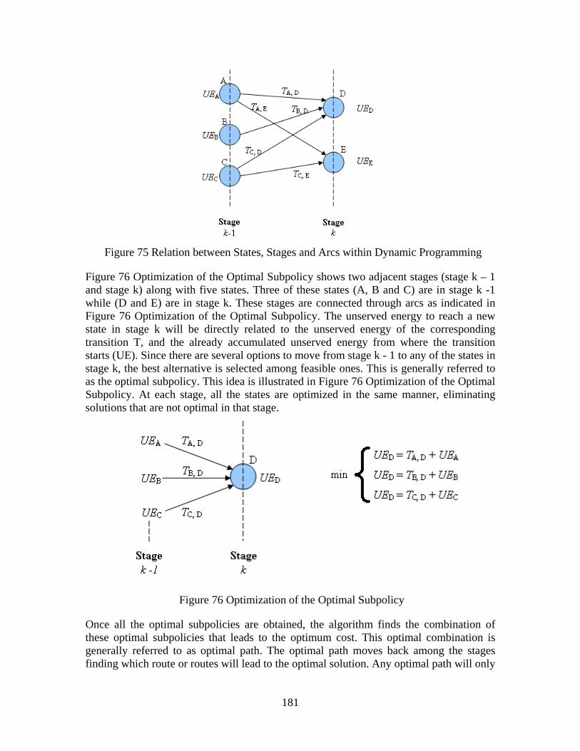
181

Figure 75 Relation between States, Stages and Arcs within Dynamic Programming

Figure 76 Optimization of the Optimal Subpolicy shows two adjacent stages (stage k – 1 and stage k) along with five states. Three of these states (A, B and C) are in stage k -1 while (D and E) are in stage k. These stages are connected through arcs as indicated in Figure 76 Optimization of the Optimal Subpolicy. The unserved energy to reach a new state in stage k will be directly related to the unserved energy of the corresponding transition T, and the already accumulated unserved energy from where the transition starts (UE). Since there are several options to move from stage k - 1 to any of the states in stage k, the best alternative is selected among feasible ones. This is generally referred to as the optimal subpolicy. This idea is illustrated in Figure 76 Optimization of the Optimal Subpolicy. At each stage, all the states are optimized in the same manner, eliminating solutions that are not optimal in that stage.

Figure 76 Optimization of the Optimal Subpolicy

Once all the optimal subpolicies are obtained, the algorithm finds the combination of these optimal subpolicies that leads to the optimum cost. This optimal combination is generally referred to as optimal path. The optimal path moves back among the stages finding which route or routes will lead to the optimal solution. Any optimal path will only

182

be composed of optimal subpolicies. Figure 77 Optimal Path in Dynamic Programming illustrates this.

Figure 77 Optimal Path in Dynamic Programming

C.2.1 Objective Function The objective function of the distribution restoration algorithm minimizes either the unserved energy of the system (UE) or the outage cost (CUE). This is performed by examining the feeders and determining when it is appropriate to energize them in order to obtain an optimal restoration plan. The general objective of distribution restoration can be expressed as

∑=

×N

iii tP

1min 105

when minimizing unserved energy or

( )∑=

××FN

iiiii tPtC

1min 106

when minimizing the outage cost. In both cases, Pi is the expected load of the ith feeder, ti the restoration time of the ith load and N the total number of feeders or substations. In addition, Ci represents the unserved energy cost function of the ith feeder. The above expressions account for the optimal path minimization process.

In addition, each stage solves a minimization problem that guarantees that all the paths of every stage are optimal. This minimization problem may be stated as

183

{ }kiii SSS ,,,min 21 107

where kiS represents the ith state and k is the number of transitions that lead to that state.

This minimization process is repeated for all states of a stage, and all stages obtaining only optimal subpolicies.

C.2.2 Constraint Modeling Power balance constraint: The power balance constraint is met by determining the instant at which a feeder combination (or state) will match the expected available generation curve. This load-generation match returns the time at which the equality constraint is satisfied. This is taken to be the optimal restoration time of the state. This ensures that all tested combinations will satisfy the power balance equality constraint. The restoration time obtained from the power balance constraint is used to calculate the unserved energy of the arc, that is, the unserved energy of the feeder in queue to be energized.

Frequency deviation: Since DSR takes place after some generation has been synchronized to the system, the complete set of loads can be screened for compliance before proceeding with the optimization process. The states that are not able to meet such criteria are removed from consideration.

C.3 Dynamic Programming Based Distribution Restoration Algorithm The dynamic programming based distribution restoration algorithm is composed of several key functions that complement the standard dynamic programming formulation. It mainly consists of a continuous computation of unserved energy or cost once the power balance equality constraint is satisfied. Although the relaxed version of the power balance constraint may be used, this results in a less optimal solution.

As previously mentioned, the number of stages is determined by the total number of feeders to be energized. State and arcs computation is performed by first determining the number of different feeders (i.e. different load levels) available in the optimization process, obtaining the optimal combination for stage 1, and then adding the matrix of different feeders to each of the optimal combinations of stage 1. The resulting data matrix of stage 2 is sorted based on the states or load levels created. If there are one or more alternatives for any load level, the combination that results in a minimum value is selected obtaining what is called the optimal subpolicy. The process is repeated until all stages have been carried out.

In the event that 2 or more feeders have the same load level, this is specified as one transition that may happen several times depending on the number of feeders that share the same load level. Figure 78 Dynamic Programming Based Distribution System Restoration illustrates the general algorithm.

C.4 State Reduction in Dynamic Programming During an optimization process, some of the states of a particular stage may be ‘close’ to each other. This proximity allows some of these states to be removed from the optimization process, thus speeding up the computation. The clustering strategy identifies

184

and groups these states and selects the one with the best performance. The states that are redundant due to proximity are discarded from the optimization process.

State reduction, also known as aggregation, improves the performance of dynamic programming by solving a relaxation of the original problem. Since the problem solved is an approximation a global optimal solution to the problem is not guaranteed.

Input data

LoadGeneration

Rank

Set i to 1Compute states for stage i

Determine rest. timeCompute obj. Function

i > NS

i = i + 1

END

No

Yes

Compute states for stage iDetermine rest. time

Compute obj. function

Determine number of stages (NS)

Find optimal path through backward DP

Figure 78 Dynamic Programming Based Distribution System Restoration

State reduction is an additional procedure added to the basic dynamic programming algorithm. This procedure is performed at each stage after the corresponding states are computed. State reduction groups those states that can be considered ‘close’ to each other with the purpose of speeding up the optimization process. The algorithm for the state reduction subroutine is illustrated in Figure 78 Dynamic Programming Based Distribution System Restoration.

185

In the state reduction process, groups are constructed using a user-defined parameter. After the states of a stage are generated, these are sorted from minimum to maximum in relation to the corresponding amount of restored power. The algorithm then proceeds to create the groups by adding to the first state (minimum power restored) the user defined parameter. All states that are within the group range are clustered and the one that has better performance is selected to represent the group in the remaining of the optimization process. The algorithm selects the next state that does not lie within the group and repeats the clustering and selection process. Each of these steps is illustrated in Figure 79 State Reduction Flow Diagram for Basic Functions.

The effectiveness of clustering is dependent on the size of the group. A large group size will eliminate a large number of the states resulting in faster algorithm performance. A small group size produces a more accurate solution.

C.5 Dynamic Programming Restoration Example This section shows the results of the dynamic programming restoration algorithm when tested on an illustrative example that minimizes system unserved energy. An outage cost minimization and feeder prioritization were also performed however are not shown in this appendix. The example is similar to that shown in Chapter 4, however reactive power considerations are neglected. Restoration plans are developed for a 32-feeder system similar in an arrangement similar to that of Figure 62. Observations related to the algorithm performance are shown in Section C.6.

186

Input data

Sort states (total states = N)Set k to 1

Compute cluster range (CR)

k ≤ N

State k Є CR

Store in clusterk = k + 1

Select best stateReset cluster

Compute new CRk = k + 1

ENDN

Y

N

Y

Figure 79 State Reduction Flow Diagram for Basic Functions

C.5.1 Test System Data The load data for the 32-load test system used in the example of this section is shown in Table 61 Load Data for 32-Load Test Bed. Load data such as ID and MW value are provided in Table 61 Load Data for 32-Load Test Bed. Table 62 Expected Generation Data for 32-Load Test Bed shows one expected available generation data. The generation restoration time is the time at which the indicated generation becomes available at distribution system substations.

187

Table 61 Load Data for 32-Load Test Bed

Load ID MW Load ID MW L1 5.1 L17 5 L2 7.3 L18 7.2 L3 4 L19 4.1 L4 6.4 L20 6.3 L5 8.1 L21 8 L6 9.2 L22 9.3 L7 7.4 L23 7.6 L8 4.5 L24 4.6 L9 7.5 L25 7.7 L10 3.7 L26 3.6 L11 10.2 L27 10.1 L12 5.5 L28 5.6 L13 6.7 L29 7 L14 8.5 L30 8.6 L15 6.9 L31 6.8 L16 3.5 L32 3.4

Table 62 Expected Generation Data for 32-Load Test Bed

Time (min)

Generation (MW)

Time (min)

Generation (MW)

Time (min)

Generation (MW)

0 0 40 45 199 110 5 5 51 50 239 130 8 7 56 65 290 132 12 9 64 67 305 138 15 10 76 70 340 155 20 11 91 75 370 180 25 20 111 85 390 200 28 25 136 100 400 210 35 40 164 105

C.5.2 Illustrative Distribution Restoration Examples: Unserved Energy Minimization

This example evaluates the restoration plan when the corresponding goal is to minimize the system unserved energy. The optimal restoration plan obtained from this objective function looks to improve the system operation regardless of the type of customer. This is equivalent to a fixed unserved energy cost for all the users and no priorities within the

188

system. Under these considerations, the restoration plan will be affected mainly by the system available generation and the load estimates.

In this example, the optimal solution is shown to have a strong dependency on the expected available generation of the system. The slowly increasing generation shown reaches an unserved energy value of 680.0 MWh. For comparison purposes, a random sequence that meets the desired constraints was selected. This random restoration sequence corresponds to [L12, L4, L9, L15, L10, L1, L14, L25, L20, L2, L3, L31, L17, L6, L21, L13, L16, L28, L5, L26, L7, L19, L23, L8, L29, L27, L11, L18, L30, L22, L32, L24] (Refer to table B.1 for numerical values) and results in a value of 686.2 MWh. Table 63 summarizes the results of this example.

Application of the state reduction function returned similar values to the full dynamic programming algorithm. These results depend on the group size selected and correspond to a solution that approaches the global optimal solution but may not be this solution. Since larger groups generally discard a greater amount of states, then it is more likely that the solution will worsen as the group size is increased. Nevertheless, any group may lead to the global optimal depending on the problem characteristics. As an example of solution degrading, a group size of 0.5 MW resulted in an increase of 0.3 MWh over the group size of 0.2 MW. In terms of overall solution quality, the objective function increases by 0.4% at the most for the example under study. This may be considered an adequate solution to the restoration problem.

Table 63 Results for Example I: Unserved Energy Minimization All Values in MWh

Solution method

Generation

Type

Slow

DP

Met

hods

Full DP – no grouping 680.0

Group size of 0.2 MW 680.1




Oth

ers

Random restoration 686.2

Energize small loads first 683.9

Energize large loads first 685.3

Computational time may be the most important contribution of state reduction. The results show that state reduction improves substantially the computational time. The full DP algorithm requires 1199 seconds to solve. DP with state reduction using 0.5 MW

189

groups obtains the solution in around 40 seconds which is approximately 30 times faster. A computational time comparison is shown in Figure 80 Average Computational Time as a Function of Group Size for Example I. Due to resolution of the load data, group sizes of 0.1 MW (and smaller) were not computed.

Figure 80 Average Computational Time as a Function of Group Size for Example I

C.6 Additional Computational Results

The general concern in dynamic programming is its capability to handle large systems. This problem derives from the popular curse of dimensionality. Figure 81 shows this in terms of how the computational time is affected by an increase in variable. The state reduction technique applied in this thesis reduces the computational time at the expense of some solution precision. However, this reduction is sufficient to allow the implementation of this technique up to some number of variables.

0 0.1 0.2 0.3 0.4 0.5

200

400

600

800

1000

1200

Group Size (MW)

Com

puta

tiona

l Tim

e (s

econ

ds) Trend line

190

Figure 81 Estimated Computational Time for Example I as a Function of the Number of Variables.

The modified DP stands for the dynamic programming with state reduction algorithm using a group size of 0.5 MW.

0 5 10 15 20 25 30 35

200

400

600

800

1000

1200

Com

puta

tiona

l Tim

e (s

econ

ds)

Full DP Approx. DP

Number of Variables

191

Appendix D: Dynamic Programming Based Matlab Codes

D.1 Main Code Structure This section contains the main structure of the dynamic programming based distribution restoration algorithm. The algorithm is composed of several subroutines for ease of modification.

clear clc GC [L,L1,L2,L3,G] = Input_Data(GC); % System input data R = 0.198; % Determines the group size when state reduction is considered; clg = 1; % Performs clustering 1 = yes, else = no; tic mq = sum(L1); % Determine total number of stages [T,UE,m] = firststage(G,L,L3); % Computes initial stage values IS = T; % Initial stage OP = []; loc = []; % Initializes variables that store optimal path for k=1:(mq-1) [F2,UE] = newstates(UE,IS,T,G,L1,L3,m); % Generates new states and

% arcs

W = minimizer2(F2,UE); % Determines optimal policy to reach state N if clg == 1 W = clustering(W,R); % Performes state reduction end [m1,n1]=size(W); OP = [W;OP]; loc = [m1,n1;loc];

192

IS = []; IS = [W(:,2) W(:,8:n1)]; UE = []; UE = [W(:,2) W(:,3) W(:,4)]; end B = optimalpath(OP,loc,W,G) % Determines the solution to the problem

D.2 First Stage Subroutine This section contains the code for the first stage computation. Two codes are provided one for unserved energy and one for cost minimization (example not shown).

D.2.1 Unserved Energy function [T,UE,m] = firststage(G,L,L3) % Computes initial stage % % UE = [states, UE, restoration time] states = duplicates(L); [m,n]=size(states); T = [states eye(m)]; % Transition block matrix G1 = interp1(G(:,2),G(:,1),T(:,1),'linear'); % Time calculation G2x = interp1(L3(:,1),L3(:,2),T(:,1),'linear'); % Transition rate (Price) UEx = T(:,1).*G1; %% Unserved energy matrix UE = [T(:,1) UEx.*G2x G1]; % Unserved energy matrix of initial stage

D.2.2 Cost function [T,UE,m] = firststage(G,L,TR,L4) % Computes initial stage % states = duplicates(L); [m,n]=size(states); T = [states eye(m)]; % Transition block matrix G1 = interp1(G(:,2),G(:,1),T(:,1),'linear'); % Time calculation CENS = interp1(L4(:,1),L4(:,2),T(:,1),'linear');%; % Time calculation H = [T(:,1) CENS]; P2 = interp1(TR(:,1),TR(:,2),G1,'nearest'); % Price calculation 1 P3 = interp1(TR(:,1),TR(:,3),G1,'nearest'); % Price calculation 2 AUX1 = H(:,2)==1; AUX2 = H(:,2)==2; P1 = P2.*AUX1 + P3.*AUX2; UE = [T(:,1) T(:,1).*G1.*P1 G1]; % Unserved energy matrix of initial stage

193

% End %

D.3 New States Subroutine This section contains the code for the new states and arcs computation. Two codes are provided one for unserved energy and one for cost minimization (example not shown).

D.3.1 Unserved Energy function [F2,UE] = newstates(UE,IS,T,G,L1,L3,m1) F = []; % Calculates all possible states + arcs % [mx,nx]=size(IS); for i1=1:mx for i2=1:m1 PS(i2,:) = IS(i1,:); end F1 = [PS(:,1) T(:,1) PS+T]; F = [F; F1]; end % End % % Removes infeasible arcs % [m2,n2] = size(F); for i3=m2:-1:1 if sum(F(i3,4:n2)>L1)>0 F(i3,:)=[]; end end F2 = sortrows(F,3); % End % % Calculates 'price' of arc (unserved energy) % G2 = interp1(G(:,2),G(:,1),F2(:,3),'linear'); % Transition cost (Time) G2x = interp1(L3(:,1),L3(:,2),F2(:,2),'linear'); % Transition rate (Price) G3 = interp1(UE(:,1),UE(:,2),F2(:,1),'linear'); % Cumulative value (Energy) G4 = G3 + G2.*F2(:,2).*G2x; % Total % End %

194

UE = [F2(:,3) G4 G2];

D.3.2 Cost function [F2,UE] = newstates(UE,IS,T,G,L1,m1,TR,L4) F = []; % Calculates all possible states + arcs % [mx,nx]=size(IS); for i1=1:mx for i2=1:m1 PS(i2,:) = IS(i1,:); end F1 = [PS(:,1) T(:,1) PS+T]; F = [F; F1]; end % End % % Removes infeasible arcs % [m2,n2] = size(F); for i3=m2:-1:1 if sum(F(i3,4:n2)>L1)>0 F(i3,:)=[]; end end F2 = sortrows(F,3); % End % % Calculates 'price' of arc (unserved energy) % CENS = interp1(L4(:,1),L4(:,2),F2(:,2),'linear');%; % Time calculation H = [F2(:,2) CENS]; G2 = interp1(G(:,2),G(:,1),F2(:,3),'linear'); % Transition cost (Time) G3 = interp1(UE(:,1),UE(:,2),F2(:,1),'linear'); % Cumulative value (Energy) P2 = interp1(TR(:,1),TR(:,2),G2,'nearest'); % Price calculation 1 P3 = interp1(TR(:,1),TR(:,3),G2,'nearest'); % Price calculation 2 AUX1 = H(:,2)==1; AUX2 = H(:,2)==2; P1 = P2.*AUX1 + P3.*AUX2;

195

G4 = G3 + G2.*F2(:,2).*P1; % Total % End % UE = [F2(:,3) G4 G2];

D.4 Minimizer2 Subroutine This section contains the code that optimizes each stage within dynamic programming.

function A = minimizer2(F2,UE) % Finds the optimal path when moving from stage N-1 to stage N. % % Input variables: % F2 % UE % % Output variables % A DP = 100; % Decimal point: 10 = 1 decimal point, 100 = 2 decimal points, 1000 = 3 decimal points UE(:,1) = round(UE(:,1)*DP)/DP; [m,n] = size(UE); k=1; a1 = UE(1,1); a2=UE(1,2); A(k,:) = [k UE(1,:) F2(1,:)]; for i=2:m if UE(i,1) == a1 if UE(i,2)<a2 A(k,:) = [k UE(i,:) F2(i,:)]; a2=UE(i,2); end else k = k+1; a1 = UE(i,1); a2=UE(i,2); A(k,:) = [k UE(i,:) F2(i,:)]; end end

D.5 Clustering Subroutine This section contains the code that forms the clusters and discards states according to a ‘greedy’ criterion up to that stage. Greedy criterion selects the best state of the group.

196

function B = clustering(A,R) % Finds the optimal path when moving from stage N-1 to stage N. % % Input variables: % F2 = A % UE = R % % Output variables % A = B [m,n] = size(A); A(:,2) = round(A(:,2).*10)/10; a1 = A(1,2); a2 = A(1,3); a3 = a1 + R; a4 = A(1,5); k=1; B(k,:) = [k A(1,2:n)]; for i=2:m if ((A(i,2)>=a1) & (A(i,2)<a3)) if A(i,3)<a2 B(k,:) = [k A(i,2:n)]; a2 = A(i,3); end else a1 = A(i,2); a2=A(i,3); a3 = a1 + R; a4 = A(i,5); k = k+1; B(k,:) = [k A(i,2:n)]; end end

D.6 Optimal Path Subroutine This section contains the code that finds the optimal path for the dynamic programming algorithm.

function B = optimalpath(OP,loc,W,G) B=[]; a = cumsum(loc); [m,n]=size(loc); d = W(5); e = W(6); f= W(4); B=[B;m+2-1,e,f,d]; for i=2:m

197

b=a(i-1,1)+1; c=a(i,1); A = OP(b:c,:); A(:,7)=round(A(:,7).*10)/10; e = interp1(A(:,7),A(:,6),d,'nearest'); f = interp1(A(:,7),A(:,4),d,'nearest'); d = interp1(A(:,7),A(:,5),d,'nearest'); B = [B;m+2-i,e,f,d]; end d = 0; e = B(m,4); f = interp1(G(:,2),G(:,1),e,'linear'); B=[B;1,e,f,d];

development and evaluation of system restoration ... · of system restoration strategies from a...

Documents