developing pavement distress deterioration...

Research ArticleDeveloping Pavement Distress Deterioration Models for PavementManagement System Using Markovian Probabilistic Process

Promothes Saha,1 Khaled Ksaibati,1 and Rebecca Atadero2

1Department of Civil and Architectural Engineering, University of Wyoming, Dept. 3295, 1000 E. University Ave, Laramie,WY 82071, USA

2Department of Civil and Environmental Engineering, Colorado State University, Fort Collins, CO 80523-1372, USA

Correspondence should be addressed to Promothes Saha; [email protected]

Received 1 August 2017; Revised 25 September 2017; Accepted 1 October 2017; Published 19 November 2017

Academic Editor: Ghassan Chehab

Copyright © 2017 Promothes Saha et al. 'is is an open access article distributed under the Creative Commons Attribution License,which permits unrestricted use, distribution, and reproduction in any medium, provided the original work is properly cited.

In the state of Colorado, the Colorado Department of Transportation (CDOT) utilizes their pavement management system(PMS) to manage approximately 9,100 miles of interstate, highways, and low-volume roads. 'ree types of deteriorationmodels are currently being used in the existing PMS: site-speci6c, family, and expert opinion curves. 'ese curves are de-veloped using deterministic techniques. In the deterministic technique, the uncertainties of pavement deterioration related totra8c and weather are not considered. Probabilistic models that take into account the uncertainties result in more accuratecurves. In this study, probabilistic models using the discrete-time Markov process were developed for 6ve distress indices:transverse, longitudinal, fatigue, rut, and ride indices, as a case study on low-volume roads. Regression techniques were used todevelop the deterioration paths using the predicted distribution of indices estimated from the Markov process. Resultsindicated that longitudinal, fatigue, and rut indices had very slow deterioration over time, whereas transverse and ride indicesshowed faster deterioration. 'e developed deterioration models had the coe8cient of determination (R2) above 0.84. Asprobabilistic models provide more accurate results, it is recommended that these models be used as the family curves in theCDOT PMS for low-volume roads.

1. Introduction

'e Colorado Department of Transportation (CDOT) isresponsible for maintaining a highway system that en-compasses more than 9,100 centerline miles (about 23,000total lane miles) and includes 3,437 bridges [1]. Every year,approximately $740 million is allocated to maintain thissystem. In order to maintain this system most e8ciently, theCDOTuses a pavement management system (PMS). A PMSis a strategic and systematic process to maintain and upgradethe road network. When funding is limited, the PMSidenti6es the best mix of road preservation projects thatprovides the most bene6t to society in terms of overall life-cycle cost of the road network. In the CDOT PMS, a com-posite index, known as the overall pavement index (OPI), isused as the reporting criterion for the condition of the statehighway system [2]. 'e OPI comprised a weighted com-bination of ride quality, rutting, and cracking. 'ere are

three diAerent types of cracking: transverse, longitudinal,and fatigue. 'e CDOT highway maintenance system isdivided into four categories: interstate and national highwaysystem (NHS) high volume, medium volume, and lowvolume based on the annual average daily tra8c (AADT)and annual average daily truck tra8c (AADTT) [3].'e low-volume roads consist of 2,022 centerline miles (about total5,614 lane miles).

As the performance of each roadway segment is dif-ferent, the CDOT develops a segment-speci6c deteriorationcurve. 'ese curves are generated to satisfy certain condi-tions, including at least 6ve years of historical pavementdistress data after last rehabilitation, the standard deviationof the data cannot exceed 10, and the minimum coe8cient ofregression (R2) is considered as 0.5. When these conditionsare not met, a segment-speci6c curve cannot be generated,and the family or expert opinion curves can be used. Familyor expert opinion curves are generated for some roadway

HindawiAdvances in Civil EngineeringVolume 2017, Article ID 8292056, 9 pageshttps://doi.org/10.1155/2017/8292056

mailto:[email protected]

https://doi.org/10.1155/2017/8292056

segments with similar tra8c, pavement type, and pavementthickness in a same climate area.

All these deterioration curves are generated using a de-terministic technique [3, 4]. 'e segment-speci6c perfor-mance curves can be generated for a smaller number ofsegments satisfying the required conditions [4]. Speci6cally,continuous 6ve-year distress data without any maintenancetreatment could be found for some roadway segments.Moreover, the evaluation of distress indices exceeds thestandard deviation of 10 for a signi6cant number of roadwaysegments [4]. However, as the deterministic technique doesnot take into account the uncertainties in pavement behaviorunder variable tra8c load and weather conditions [5–7],modeling uncertainty requires the use of probabilisticoperation research techniques [5, 6]. Key summaries fromthe study Butt [8] conducted about implementing a proba-bilistic technique in the pavement management system (PMS)are as follows:

(i) Predicted maintenance treatments are not 6xed,rather depend on how the pavement actuallydeteriorates.

(ii) Because of the uncertainty in selecting maintenancetreatments, the treatments should be selected witha high degree of probability.

(iii) 'e success of maintenance decisions can be eval-uated by comparing the expected and actual pro-portions of the miles in a given condition state.

(iv) 'is model has the potential for signi6cant costsaving in selecting projects satisfying the targetnetwork performance.

(v) 'is model can also be incorporated into dynamicprogramming to produce optimal solutions.

In a probabilistic technique, only two years of historicaldata are needed to develop a deterioration model. Cur-rently, the Markov process is popular among probabilistictechniques to develop a deterioration model. MichiganDOT already improved their PMS using the Markovprocess [5, 9]. In this paper, the Markov process was ap-plied to the low-volume roads of Colorado to developdeterioration models. 'ese deterioration models can beused to replace the family curves CDOT currently uses fortheir PMS.

2. CDOT Pavement Deterioration Model

'e CDOT pavement management software uses 6ve dis-tress indices to model pavement deterioration: threecracking indices (transverse, longitudinal, and fatigue),roughness, and rutting indices. When all the values areloaded into the software, it generates deterioration curves forall roadway segments. For each segment, 6ve performancecurves are generated for each of the distress indices. 'eseperformance curves are named as the site-speci6c curves.'ere are two other types of performance curves: pavementfamily and expert opinion. 'e most desirable of these is thesite-speci6c curve. When site-speci6c curves are not avail-able, family or expert opinion curves can be used.

2.1. Site-Speci+c Curves. 'e length of the CDOT roadwaysegments ranges from 0.5 mile to 5 miles. For each segment,a site-speci6c performance curve is generated using his-torical distress data as discussed earlier.

2.2. Family of Curves. 'e CDOTuses the following criteriato de6ne the family curve:

(i) Pavement types: asphalt, asphalt over concrete,concrete, and concrete over asphalt

(ii) Tra8c: low, medium, high, very high, and very veryhigh

(iii) Climate: very cold, cold, moderate, and hot(iv) Pavement thickness (asphalt: 0 to 4 inches, 4 to 6

inches, and greater than 6 inches; concrete: pave-ments less than 8 inches and greater than 8 inches)

'ese categories allow for 200 pavement families. Atleast 9 points are needed to generate a family curve.

2.3. Expert Opinion Curves. When neither site-speci6c norfamily curves are available, an expert opinion curve isassigned. 'e expert opinion curves are generated for eachpavement family. As there were 200 pavement families, 200curves were generated. 'ese curves were not developedfrom regression analysis of data, rather are derived fromexpert opinion. 'ese curves are least desirable for anypavement segment [4].

3. Literature Review

In the PMS, the pavement deterioration model (PDM) is thekey to making maintenance strategies and allocating fundingfor the future. An accurate and reliable PDM is essential forthe optimization model of the PMS [10]. Many researchershave attempted to develop a PDM using diAerent techniques[5, 6, 8, 9, 11, 12]. 'ese techniques can be divided intotwo main types—namely, deterministic and probabilisticmodels.

3.1.DeterministicPavementDeteriorationModel. Deterministicmodeling techniques are the most common because of theirrelative simplicity, ease of use, and familiarity [5, 6]. 'esetechniques include straight-line extrapolation, S-shapedcurves, polynomial constrained least squares, and logisticgrowth models [13]. Silva et al. [5] discussed the advantagesand disadvantages of the deterministic models. 'e disad-vantages are as follows:

(i) Models do not take into account the uncertainties inpavement behavior under variable tra8c load andweather conditions.

(ii) Developing models require an accurate and abun-dant dataset. Accuracy of datasets can be greatlyaAected by regular maintenance or minor re-habilitation activities.

(iii) It is necessary to include all confounding variablesthat aAect pavement deterioration.

2 Advances in Civil Engineering

�e critical disadvantage of deterministic models is thatit does not take into account the uncertainties [5–7].Modeling uncertainty requires the use of probabilistic op-eration research techniques [5, 6].

3.2. Probabilistic Pavement DeteriorationModel. In the early1970s, the applications of probabilistic models for modelingpavement performance were �rst discussed [5]. Among theprobabilistic models, the Markov model is currently beingimplemented in modeling pavement performance. Manyresearch attempted to develop the pavement performancemodel using the Markov process [5, 6, 8, 14–17]. Sure-ndrakumar et al. [6] used the Markov process to developa decision support system for pavement maintenancemanagement. In this study, a Poisson distribution has beenused in developing state transition matrices. Butt [8] studiedthe advantages of using a Markov process in the pavementmanagement system (PMS). A critical component of theMarkov model is the transition probability matrix (TPM).Generally, the TPM is calculated based on the historicalpavement condition data [15]. �e Markov process can bede�ned in a discrete or continuous time with a countablestate space. In order to explain a discrete-time Markovprocess, consider a road for which the condition is observedat year 0, 1, 2, . . ., n. Let Xn be the condition at year n forn� 0, 1, 2, . . ..Xn can be denoted as the state of the process attime n, withX0 denoting the initial state. IfXn takes values ina discrete space such as Z � {1, 2, . . . , 100}, then the processis said to be discrete-valued.

3.3. Formulation of the Distress Indices. According to theCDOT, the distress indices are scaled from 0 to 100,where 100 represents a �awless pavement with no dis-tresses and 0 represents the worst condition. Transverse,longitudinal, and fatigue cracking indices can be calcu-lated for each roadway segment using (1), while roughnessand rut indices can be calculated with (2) and (3),respectively.

Distress index � 100 1−DistressLOWMaxLOW

−DistressMID

MaxMID(

−DistressHIGH

MaxHIGH), (1)

Ride index � 100∗ 1−IRIavg −Amin

Bmax( ), (2)

Rut index � 100∗ 1−Rutavg −Bmin

Bmax −Bmin( ), (3)

where (i) DistressLOW,DistressMID, and DistressHIGH arelow, median, and high values of fatigue, transverse, andlongitudinal cracking, respectively, and (ii) IRIavg and Rutavgare average IRI and rut depth, respectively.

�e values of all other parameters in (1)–(3) can be foundin Table 1.

4. Methodology

�e Markov model provides a prediction of pavementperformance. Pavement performance can be determined byeach distress index or a combined index representing theoverall pavement condition. Most commonly used pave-ment distress indices are transverse, fatigue, longitudinalcracking, roughness, and ride. Usually, these indices rangefrom 0 to 100, where 100 represents the best condition and0 is for the worst condition. A pavement section begins itslife in a near-perfect condition. Over the years, the pave-ment condition deteriorates due to many factors such astra�c loading and weather conditions. Most states evaluatetheir pavement condition once a year. In order to developa capital improvement plan (usually a �ve-year plan), stateagencies need to predict their pavement condition forthe next �ve years. In this section, how to predict thepavement condition for the future using the Markov modelis discussed.

Markov models start with developing a transition prob-ability matrix (TPM). A TPM represents the probability thata segment will stay in a speci�c condition for a speci�c year.For example, Table 2 represents a TPM of a roadway network[6, 7, 18]. It was assumed that the pavement condition rangesfrom 1 to 5, where 5 represents the best condition and 1 is forthe worst. In this table, p(j) is the probability that a segmentwill stay in condition j(j � 1, 2, . . . , 5). p(j) is calculated bythe number ofmiles at condition j divided by the total numberof miles at conditions j and j− 1.�e entry 1 in the last row ofthe table indicates a reconstruction state. �e pavementcondition cannot transit from this state at all. In this table, itwas assumed that a segment cannot degrade by more thana single condition in one year. �e reason is, from the pre-vious experience it was found that pavement does not degradethat fast.

�e next year’s pavement condition can be determinedby multiplying the initial state vector v(0) by the TPM

Table 1: �e values of parameters for calculating distress indicesfor asphalt pavement.

Fatigueindex

Transverseindex

Longitudinalindex

Rideindex

Rutindex

MaxLOW 6230 160 3802 — —MaxMID 3375 111 2492 — —MaxHIGH 2014 49 1478 — —Amin — — — 0 —Bmin — — — — 0.15Bmax — — — 26 0.95

Table 2: Transition probability matrix with �ve states [7].

To condition 5 4 3 2 1

From condition

5 p(1) 1− p(1) 0 0 04 0 p(2) 1− p(2) 0 03 0 0 p(3) 1− p(3) 02 0 0 0 p(4) 1− p(4)1 0 0 0 0 1

Advances in Civil Engineering 3

raised to the power of t, where t represents the number ofyears in the future for which the pavement condition will bedetermined.is initial state vector v(0) considers that all thesegments stay at the best condition (condition 5). In thisstudy, as the Markov chain is reserved for a process witha discrete set of times, it can be considered as a discrete-timeMarkov model. For this example, the initial vector is statedbelow:

5 4 3 2 15 1 0 0 0 0

e next year’s pavement condition can be determinedusing the following equation:

[v(1)] � [v(0)]∗[TPM],

[v(2)] � [v(0)]∗[TPM]2,⋮

[v(t)] � [v(0)]∗[TPM]t.

(4)

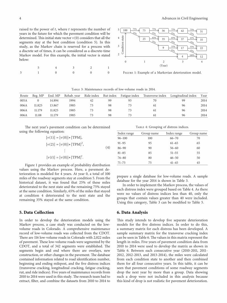
Figure 1 provides an example of probability distributionvalues using the Markov process. Here, a pavement de-terioration is modeled for 4 years. At year 0, a total of 100miles of the roadway segments stay at condition 5. From thehistorical dataset, it was found that 25% of these milesdeteriorated to the next state and the remaining 75% stayedat the same condition. Similarly, 65% of the miles that stayedat condition 4 deteriorated to the next state and theremaining 35% stayed at the same condition.

5. Data Collection

In order to develop the deterioration models using theMarkov process, a case study was conducted on the low-volume roads in Colorado. A comprehensive maintenancerecord of low-volume roads was collected from the CDOT.ere are 116 low-volume roads in Colorado with 2,022 milesof pavement. ese low-volume roads were segmented by theCDOT, and a total of 342 segments were established. esegments begin and end where there are overlays, newconstruction, or other changes in the pavement. e databasecontained information related to road identi�cation number,beginning and ending milepost, and the �ve distress indices(transverse cracking, longitudinal cracking, fatigue cracking,rut, and ride indices). Five years of maintenance records from2010 to 2014 were used in this study.e research team had toextract, �lter, and combine the datasets from 2010 to 2014 to

prepare a single database for low-volume roads. A sampledatabase for the year 2014 is shown in Table 3.

In order to implement the Markov process, the values ofeach distress index were grouped based on Table 4. As therewere no values of distress indices less than 40, only thegroups that contain values greater than 40 were included.Using this category, Table 3 can be modi�ed to Table 5.

6. Data Analysis

is study intends to develop �ve separate deteriorationmodels for the �ve distress indices. In order to do this,a summary matrix for each distress has been developed. Asample summary matrix for the transverse cracking indexcan be seen in Table 6.e values in this matrix represent thelength in miles. Five years of pavement condition data from2010 to 2014 were used to develop the matrix as shown inTable 6. Between each consecutive year (2010-2011, 2011-2012, 2012-2013, and 2013-2014), the miles were calculatedfrom each condition state to another and then combinedthem for all four consecutive years. In this table, it can beseen that pavement conditions of some roadway segmentsdrop the next year by more than a group. Data showingsuch a drop were not included in this analysis becausethis kind of drop is not realistic for pavement deterioration.

(Year)

100 75

25

75% 25% 25% 25% 25%

35% 35% 35%

45% 45%

65%

56

35

75%

65%

42

37

75%

65%

31

35

75%

22

12

55% 17

4

55%9

0 1 2 3 4

Cond

ition

stat

e

2

3

4

5

100%

Figure 1: Example of a Markovian deterioration model.

Table 3: Maintenance records of low-volume roads in 2014.

Route Beg. MP End. MP Rehab. year Ride index Rut index Fatigue index Transverse index Longitudinal index Year005A 0 14.894 1994 42 99 93 70 99 2014006A 11.825 13.867 1985 73 98 73 61 96 2014006A 11.179 11.825 1985 73 98 73 61 96 2014006A 11.08 11.179 1985 73 98 73 61 96 2014

Table 4: Grouping of distress indices.

Index range Group name Index range Group name96–100 100 66–70 7091–95 95 61–65 6586–90 90 56–60 6081–85 85 51–55 5576–80 80 46–50 5071–75 75 41–45 45


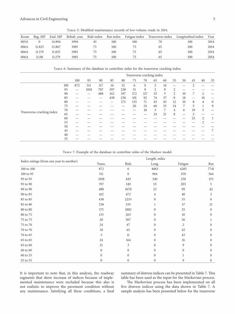
It is important to note that, in this analysis, the roadwaysegments that show increase of indices because of imple-mented maintenance were excluded because this also isnot realistic to improve the pavement condition withoutany maintenance. Satisfying all these conditions, a 6nal

summary of distress indices can be presented in Table 7.'istable has been used as the input for the Markovian process.

'e Markovian process has been implemented on all6ve distress indices using the data shown in Table 7. Asample analysis has been presented below for the transverse

Table 5: Modi6ed maintenance records of low-volume roads in 2014.

Route Beg. MP End. MP Rehab. year Ride index Rut index Fatigue index Transverse index Longitudinal index Year005A 0 14.894 1994 45 100 100 70 100 2014006A 11.825 13.867 1985 75 100 75 65 100 2014006A 11.179 11.825 1985 75 100 75 65 100 2014006A 11.08 11.179 1985 75 100 75 65 100 2014

Table 6: Summary of the database in centerline miles for the transverse cracking index.

Transverse cracking index100 95 90 85 80 75 70 65 60 55 50 45 40 35

Transverse cracking index

100 872 511 117 16 52 6 0 3 16 — — 2 — —95 — 1018 707 397 238 51 0 2 9 2 — — — —90 — — 488 412 197 172 117 33 5 2 10 7 2 —85 — — — 438 238 101 92 74 37 8 18 — 10 —80 — — — — 175 135 71 43 45 12 10 8 4 075 — — — — — 20 24 66 35 14 7 5 1 970 — — — — — — 18 3 7 4 6 19 5 —65 — — — — — — — 24 21 8 — 2 — —60 — — — — — — — — — — — 25 2 155 — — — — — — — — — — — — 2 —50 — — — — — — — — — — — — — —45 — — — — — — — — — — — — — 740 — — — — — — — — — — — — — —35 — — — — — — — — — — — — — —

Table 7: Example of the database in centerline miles of the Markov model.

Index ratings (from one year to another)Length, miles

Trans. Ride Long. Fatigue Rut100 to 100 872 0 4063 4285 7741100 to 95 511 0 964 559 56495 to 95 1018 443 340 250 15395 to 90 707 149 55 203 590 to 90 488 1670 23 99 4290 to 85 412 472 4 40 385 to 85 438 2255 8 55 085 to 80 238 535 1 37 2180 to 80 175 1882 0 25 080 to 75 135 263 0 10 075 to 75 20 307 0 56 175 to 70 24 47 0 2 070 to 70 18 65 0 42 070 to 65 3 11 0 43 065 to 65 24 164 0 16 065 to 60 21 3 0 9 060 to 60 0 0 0 0 060 to 55 0 0 0 1 055 to 55 0 0 0 9 0


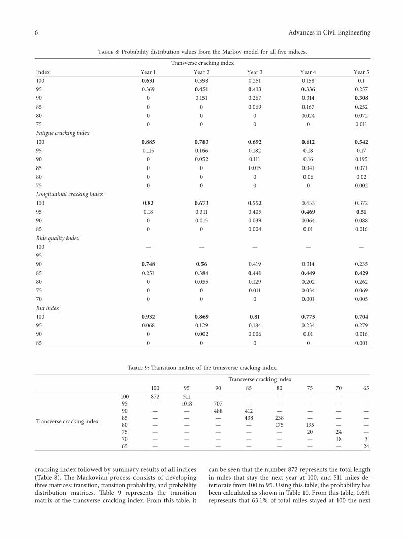
cracking index followed by summary results of all indices(Table 8). 'e Markovian process consists of developingthree matrices: transition, transition probability, and probabilitydistribution matrices. Table 9 represents the transitionmatrix of the transverse cracking index. From this table, it

can be seen that the number 872 represents the total lengthin miles that stay the next year at 100, and 511 miles de-teriorate from 100 to 95. Using this table, the probability hasbeen calculated as shown in Table 10. From this table, 0.631represents that 63.1% of total miles stayed at 100 the next

Table 8: Probability distribution values from the Markov model for all 6ve indices.

Transverse cracking indexIndex Year 1 Year 2 Year 3 Year 4 Year 5100 0.631 0.398 0.251 0.158 0.195 0.369 0.451 0.413 0.336 0.25790 0 0.151 0.267 0.314 0.30885 0 0 0.069 0.167 0.25280 0 0 0 0.024 0.07275 0 0 0 0 0.011Fatigue cracking index100 0.885 0.783 0.692 0.612 0.54295 0.115 0.166 0.182 0.18 0.1790 0 0.052 0.111 0.16 0.19585 0 0 0.015 0.041 0.07180 0 0 0 0.06 0.0275 0 0 0 0 0.002Longitudinal cracking index100 0.82 0.673 0.552 0.453 0.37295 0.18 0.311 0.405 0.469 0.5190 0 0.015 0.039 0.064 0.08885 0 0 0.004 0.01 0.016Ride quality index100 — — — — —95 — — — — —90 0.748 0.56 0.419 0.314 0.23585 0.251 0.384 0.441 0.449 0.42980 0 0.055 0.129 0.202 0.26275 0 0 0.011 0.034 0.06970 0 0 0 0.001 0.005Rut index100 0.932 0.869 0.81 0.775 0.70495 0.068 0.129 0.184 0.234 0.27990 0 0.002 0.006 0.01 0.01685 0 0 0 0 0.001

Table 9: Transition matrix of the transverse cracking index.

Transverse cracking index100 95 90 85 80 75 70 65


100 872 511 — — — — — —95 — 1018 707 — — — — —90 — — 488 412 — — — —85 — — — 438 238 — — —80 — — — — 175 135 — —75 — — — — — 20 24 —70 — — — — — — 18 365 — — — — — — — 24


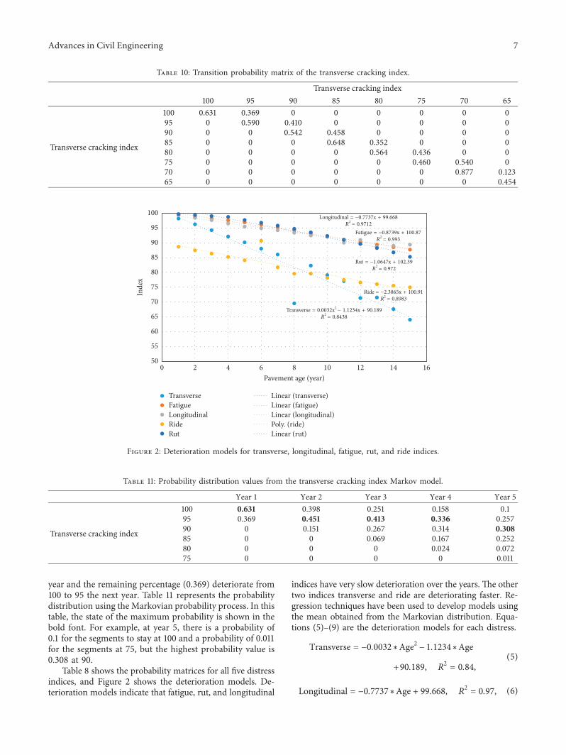
year and the remaining percentage (0.369) deteriorate from100 to 95 the next year. Table 11 represents the probabilitydistribution using the Markovian probability process. In thistable, the state of the maximum probability is shown in thebold font. For example, at year 5, there is a probability of0.1 for the segments to stay at 100 and a probability of 0.011for the segments at 75, but the highest probability value is0.308 at 90.

Table 8 shows the probability matrices for all �ve distressindices, and Figure 2 shows the deterioration models. De-terioration models indicate that fatigue, rut, and longitudinal

indices have very slow deterioration over the years. e othertwo indices transverse and ride are deteriorating faster. Re-gression techniques have been used to develop models usingthe mean obtained from the Markovian distribution. Equa-tions (5)–(9) are the deterioration models for each distress.

Transverse � −0.0032∗Age2 − 1.1234∗Age

+90.189, R2 � 0.84,

(5)

Longitudinal � −0.7737∗Age + 99.668, R2 � 0.97, (6)

Table 10: Transition probability matrix of the transverse cracking index.

Transverse cracking index100 95 90 85 80 75 70 65


100 0.631 0.369 0 0 0 0 0 095 0 0.590 0.410 0 0 0 0 090 0 0 0.542 0.458 0 0 0 085 0 0 0 0.648 0.352 0 0 080 0 0 0 0 0.564 0.436 0 075 0 0 0 0 0 0.460 0.540 070 0 0 0 0 0 0 0.877 0.12365 0 0 0 0 0 0 0 0.454

Inde

x

100

95

90

85

80

75

70

65

60

55

500 2 4 6 8 10 12 14 16

Pavement age (year)

Transverse

Ride

Fatigue

Rut

LongitudinalLinear (fatigue)Linear (longitudinal)

Linear (transverse)

Linear (rut)Poly. (ride)

Rut = 1.0647x + 102.39R

2= 0.972

Longitudinal = 0.7737x + 99.668R

2= 0.9712

Ride = 2.3865x + 100.91R

2= 0.8983

Transverse = 0.0032x2 1.1234x + 90.189R

2= 0.8438

Fatigue = 0.8739x + 100.87R

2= 0.993

Figure 2: Deterioration models for transverse, longitudinal, fatigue, rut, and ride indices.

Table 11: Probability distribution values from the transverse cracking index Markov model.

Year 1 Year 2 Year 3 Year 4 Year 5


100 0.631 0.398 0.251 0.158 0.195 0.369 0.451 0.413 0.336 0.25790 0 0.151 0.267 0.314 0.30885 0 0 0.069 0.167 0.25280 0 0 0 0.024 0.07275 0 0 0 0 0.011


Ride � −2.3865∗Age + 100.91, R2 � 0.90, (7)

Rut � −0.7737∗Age + 99.67, R2 � 0.97, (8)

Fatigue � −1.0647∗Age + 102.39, R2 � 0.97, (9)

where age indicates the age of the pavement after lastrehabilitation.

7. Conclusions

In the state of Colorado, the CDOT utilizes their PMS tokeep track of approximately 9,100 miles of interstate,highways, and low-volume roads. 'ree types of de-terioration curves are used in their PMS: site-speci6c, family,and expert opinion curves. 'ese curves are developed usingdeterministic techniques. Within the deterministic tech-nique, the uncertainties of pavement deterioration relatedto tra8c and weather are not considered. Probabilisticmodels that take into account the uncertainties resultin more accurate curves. In this research, probabilisticmodels have been developed for 6ve distress indices:transverse, longitudinal, fatigue, rut, and ride indices, asa case study on low-volume roads. Deterioration modelswere developed for 15 years to investigate the deteriorationin long-term durations. As probabilistic models providemore accurate results, it is recommended that these modelsbe used as the family curves in the CDOT PMS after minormodi6cations.

'e developed models can be highlighted as follows:

(1) Tailored speci6cally to low-volume roads.(2) As this methodology incorporates uncertainties, the

developed models’ results are more accurate thanthose currently used by the deterministic technique.

(3) 'is methodology can also be implemented on otherfunctional classes of roadways in Colorado and forother states with minor changes that reJect localconditions.

8. Recommendations

DOTs are always shifting practices to better optimize limitedresources. It was demonstrated in this paper that the de-terioration models using the Markovian probability processcan help DOTs better manage their pavements. It is rec-ommended that a comprehensive study be conducted todetermine the long-term implications of replacing de-terministic models with Markov models in the state ofColorado. It is also recommended that other DOTs considerMarkov probability processes when it comes to allocatingresources or comparing maintenance and rehabilitationstrategies within their jurisdictions.

Conflicts of Interest

'e authors declare that there are no conJicts of interestregarding the publication of this paper.

Acknowledgments

'e authors would like to thank the CDOT for supportingthis research study.

References

[1] CDOT, “Proposed budget allocation plan,” 2015, https://www.codot.gov/business/budget/cdot-budget/draft-budget-documents/fy-2015-2016-cdot-proposed-narrative-budget/view.

[2] M. Keleman, S. Henry, A. Farrokhyar, and C. Stewart,Pavement Management Manual, Colorado Department ofTransportation, Denver, CO, USA, 2005.

[3] L. Redd, CDOT’s Risk-Based Asset Management Plan,Colorado Department of Transportation, Denver, CO, USA,2013.

[4] CDOT, “Pavement management manual,” 2008, https://www.codot.gov/content/projects/I-70-East-Draft-4/Schedule%2029/Schedule%2011%20-%20Operations%20and%20Maintenance/29.11.04%20CDOT%20Pavement%20Management%20Manual.pdf.

[5] F. Silva, T. Van Dam, W. Bulleit, and R. Ylitalo, “Proposedpavement performance models for local governmentagencies in Michigan,” Transportation Research Record:Journal of the Transportation Research Board, vol. 1699,pp. 81–86, 2000.

[6] K. Surendrakumar, N. Prashant, and P. Mayuresh, “Applicationof Markovian probabilistic process to develop a decisionsupport system for pavement maintenance management,”International Journal of Scienti+c and Technology Research,vol. 2, no. 8, pp. 225–303, 2013.

[7] A. A. Butt, M. Y. Shahin, S. H. Carpenter, andJ. V. Carnahan, “Application of Markov process to pave-ment management at network level,” in Proceedings of 3rdInternational Conference on Managing Pavements, SanAntonio, TX, USA, 1994.

[8] A. A. Butt, “Application of Markov process to pavementmanagement systems at the network level,” Ph.D. thesis,University of Illinois at Urbana-Champaign, Champaign, IL,USA, 1991.

[9] W. H. Kuo, Pavement Performance Models for PavementManagement System of Michigan Department of Trans-portation, Michigan Department of Transportation, Lansing,MI, USA, 1995.

[10] S. Akyildiz, “Development of new network-level optimizationmodel for Salem district pavement management pro-gramming,” M.S. thesis, Virginia Tech, Blacksburg, VA, USA,2008.

[11] M. Y. Shahin, Pavement Management for Airports, Roadsand Parking Lots, Chapman & Hall, New York, NY, USA,1994.

[12] N. Li, R. Haas, and W. C. Xie, “Investigation of relationshipsbetween deterministic and probabilistic prediction models inpavement management,” Transportation Research Record: AJournal of Transportation Research Board, vol. 1592, pp. 70–79,1997.

[13] J. M. de la Garza, S. Akyildiz, D. R. Bish, and D. A. Krueger,“Development of network-level linear programmingoptimization for pavement maintenance programming,” inProceedings of the International Conference on Computingin Civil and Building Engineering, Nottingham, UK, 2010.

[14] K. A. Abaza, “Expected performance of pavement repairworks in a global network optimization model,” Journal ofInfrastructure Systems, vol. 13, no. 2, pp. 124–134, 2007.


https://www.codot.gov/business/budget/cdot-budget/draft-budget-documents/fy-2015-2016-cdot-proposed-narrative-budget/view



https://www.codot.gov/content/projects/I-70-East-Draft-4/Schedule%2029/Schedule%2011%20-%20Operations%20and%20Maintenance/29.11.04%20CDOT%20Pavement%20Management%20Manual.pdf




[15] A. Bako, E. Klafszky, T. Szantai, and L. Gaspar, “Optimi-zation techniques for planning highway pavementimprovements,” Annals of Operations Research, vol. 58, no. 1,pp. 55–66, 1995.

[16] X. Chen, S. Hudson, M. Pajoh, and W. Dickinson, “Devel-opment of new network optimization model for OklahomaDepartment of Transportation,” Transportation Research Re-cord: Journal of the Transportation Research Board, vol. 1524,pp. 103–108, 1996.

[17] K. Golabi, R. B. Kulkarni, and G. B. Way, “A statewidepavement management system,” Interfaces, vol. 12, no. 6,pp. 5–21, 1982.

[18] K. A. Abaza, “Back-calculation of transition probabilities forMarkovian-based pavement performance prediction models,”International Journal of Pavement Engineering, vol. 17, no. 3,pp. 253–264, 2016.


RoboticsJournal of

Hindawi Publishing Corporationhttp://www.hindawi.com Volume 2014


Active and Passive Electronic Components

Control Scienceand Engineering

Journal of


International Journal of

RotatingMachinery


Hindawi Publishing Corporation http://www.hindawi.com

Journal of

Volume 201

Submit your manuscripts athttps://www.hindawi.com

VLSI Design



Shock and Vibration


Civil EngineeringAdvances in

Acoustics and VibrationAdvances in



Electrical and Computer Engineering

Journal of

Advances inOptoElectronics

Hindawi Publishing Corporation http://www.hindawi.com

Volume 2014

The Scientific World JournalHindawi Publishing Corporation http://www.hindawi.com Volume 2014

SensorsJournal of


Modelling & Simulation in EngineeringHindawi Publishing Corporation http://www.hindawi.com Volume 2014


Chemical EngineeringInternational Journal of Antennas and

Propagation




Navigation and Observation



DistributedSensor Networks


developing pavement distress deterioration...

Documents