www.senergyworld.com

Deterministic Petrophysics

2

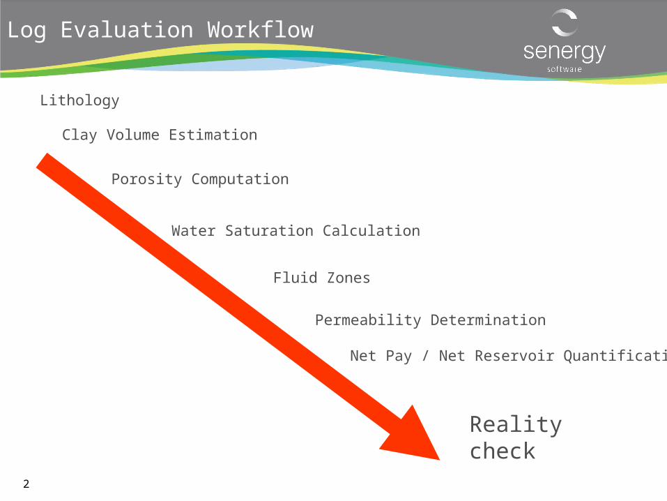
Log Evaluation Workflow

Lithology

Clay Volume Estimation

Porosity Computation

Water Saturation Calculation

Fluid Zones

Permeability Determination

Net Pay / Net Reservoir Quantification

Reality check

3

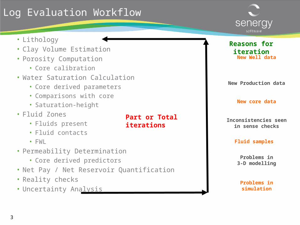
Log Evaluation Workflow

• Lithology• Clay Volume Estimation• Porosity Computation

• Core calibration

• Water Saturation Calculation• Core derived parameters• Comparisons with core• Saturation-height

• Fluid Zones• Fluids present• Fluid contacts• FWL

• Permeability Determination• Core derived predictors

• Net Pay / Net Reservoir Quantification• Reality checks• Uncertainty Analysis

Part or Total iterations

New Well data

New Production data

New core data

Inconsistencies seen in sense checks

Fluid samples

Problems in 3-D modelling

Problems in simulation

Reasons for iteration

4

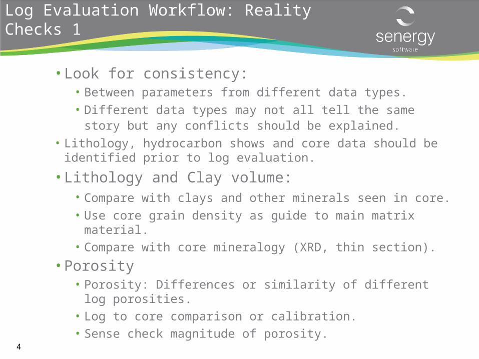
• Look for consistency: • Between parameters from different data types.

• Different data types may not all tell the same story but any conflicts should be explained.

• Lithology, hydrocarbon shows and core data should be identified prior to log evaluation.

• Lithology and Clay volume:• Compare with clays and other minerals seen in core. • Use core grain density as guide to main matrix material.

• Compare with core mineralogy (XRD, thin section).

• Porosity

• Porosity: Differences or similarity of different log porosities.

• Log to core comparison or calibration.

• Sense check magnitude of porosity.

Log Evaluation Workflow: Reality Checks 1

5

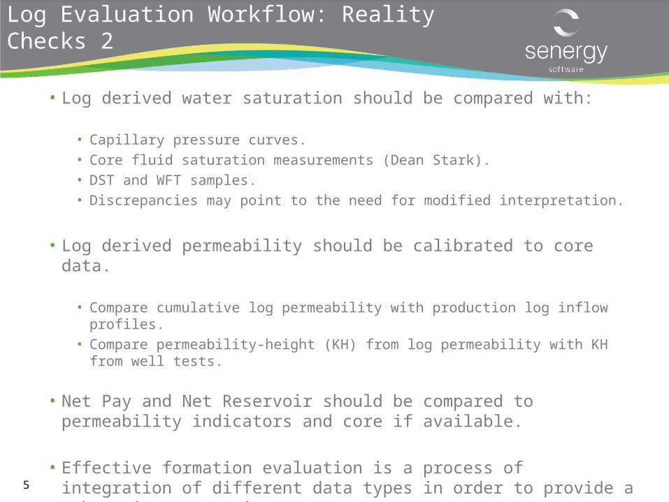
• Log derived water saturation should be compared with:

• Capillary pressure curves.• Core fluid saturation measurements (Dean Stark). • DST and WFT samples.• Discrepancies may point to the need for modified interpretation.

• Log derived permeability should be calibrated to core data.

• Compare cumulative log permeability with production log inflow profiles.• Compare permeability-height (KH) from log permeability with KH from well tests.

• Net Pay and Net Reservoir should be compared to permeability indicators and core if available.

• Effective formation evaluation is a process of integration of different data types in order to provide a robust interpretation.

Log Evaluation Workflow: Reality Checks 2

www.senergyworld.com

Deterministic Petrophysics: Lithology & Clay Volume

7

Basic Interpretation Workflow Lithology Interpretation

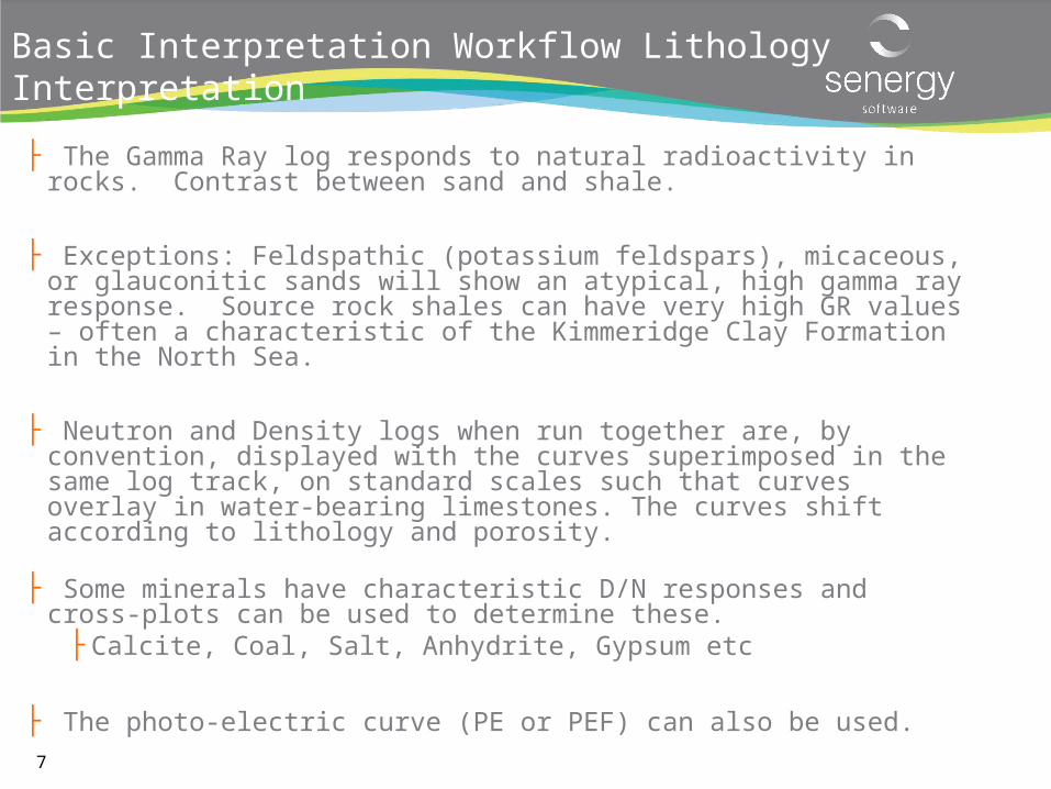
├ The Gamma Ray log responds to natural radioactivity in rocks. Contrast between sand and shale.

├ Exceptions: Feldspathic (potassium feldspars), micaceous, or glauconitic sands will show an atypical, high gamma ray response. Source rock shales can have very high GR values – often a characteristic of the Kimmeridge Clay Formation in the North Sea.

├ Neutron and Density logs when run together are, by convention, displayed with the curves superimposed in the same log track, on standard scales such that curves overlay in water-bearing limestones. The curves shift according to lithology and porosity.

├ Some minerals have characteristic D/N responses and cross-plots can be used to determine these.

├Calcite, Coal, Salt, Anhydrite, Gypsum etc

├ The photo-electric curve (PE or PEF) can also be used.

8

Shale

Sandstone

Limestone(Reference)

Dolomite

Anhydrite

Gypsum

Salt

Gas Effect

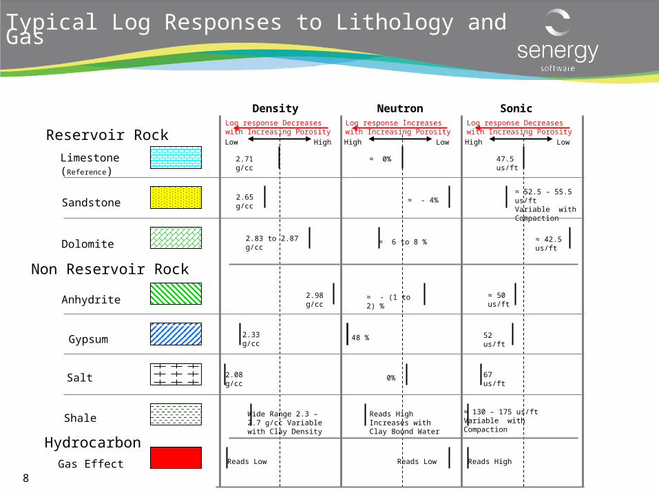
Density Neutron SonicLog response Decreaseswith Increasing Porosity

2.65g/cc

≈ - 4%≈ 52.5 – 55.5us/ftVariable with Compaction

2.71g/cc

≈ 0% 47.5us/ft

2.98g/cc

≈ - (1 to 2) %

Log response Increases with Increasing Porosity

Log response Decreaseswith Increasing Porosity

≈ 50us/ft

≈ 42.5us/ft

≈ 6 to 8 %2.83 to 2.87g/cc

2.33g/cc

48 % 52us/ft

2.08g/cc

0% 67us/ft

Wide Range 2.3 – 2.7 g/cc Variable with Clay Density

Reads HighIncreases with Clay Bound Water

≈ 130 – 175 us/ftVariable with Compaction

Reads Low Reads HighReads Low

Reservoir Rock

Non Reservoir Rock

Hydrocarbon

Low High High Low High Low

Typical Log Responses to Lithology and Gas

9

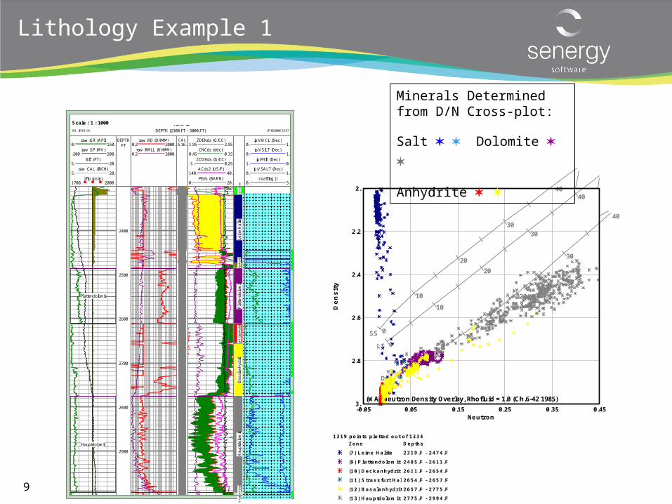
Lithology Example 1

3.

2.8

2.6

2.4

2.2

2.

Density

-0.05 0.05 0.15 0.25 0.35 0.45Neutron

SS 0

10

20

30

40

LS 0

10

20

30

40

DOL 0

10

20

30

40

(WA) Neutron Density Overlay, Rhofluid = 1.0 (Ch.6-42 1985)

1319 points plotted out of 1334Zone Depths

(7) Leine Halite 2319.F - 2474.F

(9) Plattendolomit 2485.F - 2611.F

(10) Deckanhydrit 2611.F - 2654.F

(11) Strassfurt Halite2654.F - 2657.F

(12) Basalanhydrit 2657.F - 2775.F

(13) Hauptdolomit 2775.F - 2994.F

41/8-2Scale : 1 : 1000

DEPTH (2300.FT - 3000.FT) 07/03/2006 15:47DB : IPDB (4)

raw :GR (API)0. 150.

raw :SP (MV)-200. 200.

BIT (FT)5. 20.

raw :CAL (INCH)5. 20.

rftp (psia)1700. 2000.

DEPTHFT

raw :RD (OHMM)0.2 2000.

raw :RMLL (OHMM)0.2 2000.

CAL6.16.

ZDENds (G/CC)1.95 2.95

CNCds (dec)0.45 -0.15

ZCORds (G/CC)-1. 0.25

ACds2 (US/F)140. 40.

PEds (BARN)0. 20.

ip:VWCL (Dec)0. 1.

ip:VSILT (Dec)0. 1.

ip:PHIE (Dec)1. 0.

ip:VSALT (Dec)0. 1.

coalf lag ()0. 3.

Plattendolomit

Hauptdolomit

2400

2500

2600

2700

2800

2900

Rot

er S

altz

onLe

ine

Hal

iteH

aupt

anhy

drit

Pla

ttend

olom

itD

ecka

nhyd

rit

Stra

ssfu

rt H

alite

Bas

alan

hydr

itH

aupt

dolo

mit

Wer

raan

hydr

it

Sea Bed

Minerals Determined from D/N Cross-plot:

Salt Dolomite

Anhydrite

10

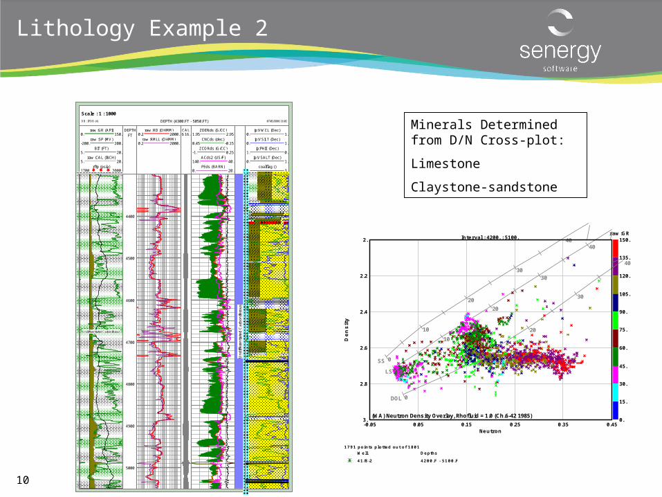
Lithology Example 2

Interval : 4200. : 5100.

3.

2.8

2.6

2.4

2.2

2.

Density

-0.05 0.05 0.15 0.25 0.35 0.45Neutron

0.

15.

30.

45.

60.

75.

90.

105.

120.

135.

150.raw:GR

SS 0

10

20

30

40

LS 0

10

20

30

40

DOL 0

10

20

30

40

(WA) Neutron Density Overlay, Rhofluid = 1.0 (Ch.6-42 1985)

1791 points plotted out of 1801Well Depths

41/8-2 4200.F - 5100.F

41/8-2Scale : 1 : 1000

DEPTH (4300.FT - 5050.FT) 07/03/2006 16:02DB : IPDB (4)

raw :GR (API)0. 150.

raw :SP (MV)-200. 200.

BIT (FT)5. 20.

raw :CAL (INCH)5. 20.

rftp (psia)1700. 2000.

DEPTHFT

raw :RD (OHMM)0.2 2000.

raw :RMLL (OHMM)0.2 2000.

CAL6.16.

ZDENds (G/CC)1.95 2.95

CNCds (dec)0.45 -0.15

ZCORds (G/CC)-1. 0.25

ACds2 (US/F)140. 40.

PEds (BARN)0. 20.

ip:VWCL (Dec)0. 1.

ip:VSILT (Dec)0. 1.

ip:PHIE (Dec)1. 0.

ip:VSALT (Dec)0. 1.

coalf lag ()0. 3.

Undifferentiated Carboniferous

4400

4500

4600

4700

4800

4900

5000

Und

iffer

entia

ted

Car

boni

fero

us

Sea Bed

9 5/8" Csg Shoe @ 3390 ft

FMT Gradient = 0.474 psia/ft . Sample results similar to mud filtrate.

Minerals Determined from D/N Cross-plot:

Limestone

Claystone-sandstone

11

Clay Volume Determination from Wire-line Logs

• Clay Volume (Vclay)

• The clay content reflects the amount of clay minerals present in a rock. The term ‘SHALE’ normally denotes assemblages of ‘clay grade’ particle sizes which include clay minerals as well as other minerals such as quartz, mica etc. The proportion of clay in ‘shale’ can range from 50 to 100%.

• Clay volume is estimated to determine:

• Shale / Sand ratios.• Shale corrections in porosity determination.• Shale corrections to Sw .• Log facies.• Reservoir Delineation.

12

Clay Volume Determination from Wire-line Logs

• Commonly used Clay Indicators are:• GR.• SP.• Resistivity (in hydrocarbon-bearing reservoir).• Neutron-Density log Cross Plot.

• Typically determine Vclay using several alternative methods and use either the minimum or average value of them

• Care required:• If radioactive minerals (other than clays) occur in sands VclayGR is an overestimate. • If hydrocarbon type is gas VclayDN is an underestimate.

• The Vclay from logs should be calibrated or compared with core data where possible:

• Shale count observed in core.• Thin section point count data.• XRD data.

13

Clay Volume from Gamma Ray VclayGR

• Normally shales contain radioactive minerals and sands do not.

• Sands may contain radioactive minerals e.g. Biotite, Potassium feldspars or Glauconite. Need corroboration with other clay indicators.

• Select ‘clay’ and ‘clean sand’ lines.

• A linear relationship is normally assumed (non-linear versions Larinov or Clavier used in FSU for older rocks).

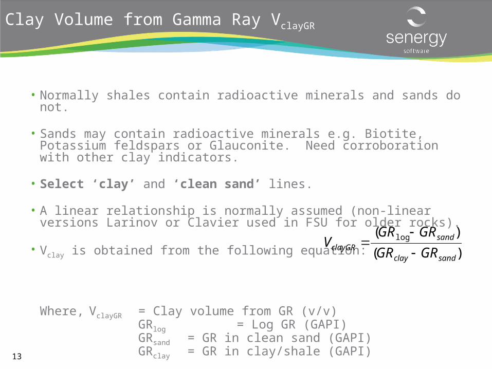
• Vclay is obtained from the following equation:

Where, VclayGR = Clay volume from GR (v/v)GRlog = Log GR (GAPI)GRsand = GR in clean sand (GAPI)GRclay = GR in clay/shale (GAPI)

)(

)( log

sandclay

sandclayGR GRGR

GRGRV

14

Clay Volume from Gamma Ray: Thin Beds

• Heterogeneity – Thin Bed Problem

In rock beds less than 2 feet thick, log resolution starts to have an impact by being strongly influenced by adjacent beds.

Thinly laminated sand-shale sequences can have clean sands, which are not resolved and are interpreted as ‘shaley’ sands or shales.

Note: This problem is not limited to shale volume detection and the GR log. Similar effects with respect to non-resolution of thin beds also occur with porosity and resistivity tools.

15

Clay Volume from Gamma Ray – Plot illustrating picking sand and clay GR

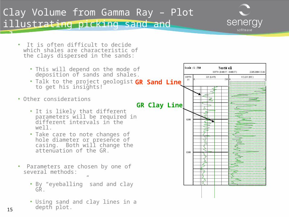
• It is often difficult to decide which shales are characteristic of the clays dispersed in the sands:

• This will depend on the mode of deposition of sands and shales.

• Talk to the project geologist to get his insights!

• Other considerations

• It is likely that different parameters will be required in different intervals in the well.

• Take care to note changes of hole diameter or presence of casing. Both will change the attenuation of the GR.

• Parameters are chosen by one of several methods:

• By “eyeballing” sand and clay GR.

• Using sand and clay lines in a depth plot.

• Note: GRsand <= the smallest Log GRlog and GRclay< largest GRlog .

Test WellScale : 1 : 750

22/05/2004 15:02DEPTH (8100.FT - 8400.FT)

DEPTHFT

GR (GAPI)0. 150.

VCLGR (DEC)0. 1.

8200

8300

GR Sand Line

GR Clay Line

16

Clay Volume from Gamma Ray – Histogram illustrating picking sand and clay GR

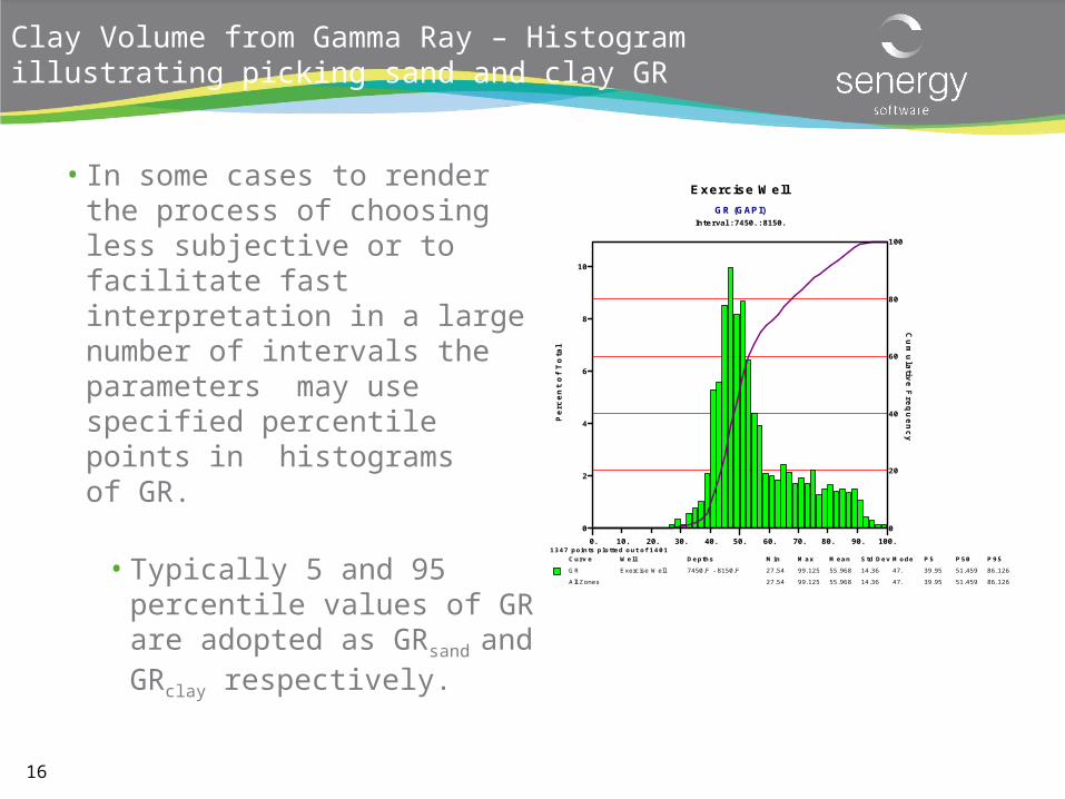
• In some cases to render the process of choosing less subjective or to facilitate fast interpretation in a large number of intervals the parameters may use specified percentile points in histogramsof GR.

• Typically 5 and 95 percentile values of GR are adopted as GRsand and GRclay respectively.

Exercise WellGR (GAPI)

Interval : 7450. : 8150.

0

20

40

60

80

100

Cum

ula

tive F

requency

0. 10. 20. 30. 40. 50. 60. 70. 80. 90. 100.0

2

4

6

8

10

Perc

ent of Tota

l1347 points plotted out of 1401

Curve Well Depths Min Max Mean Std DevMode P5 P50 P95

GR Exercise Well 7450.F - 8150.F 27.54 99.125 55.968 14.36 47. 39.95 51.459 86.126

All Zones 27.54 99.125 55.968 14.36 47. 39.95 51.459 86.126

17

Clay Volume from SP VclaySP

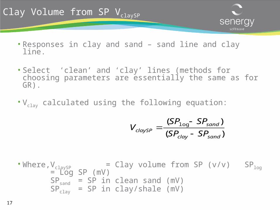
• Responses in clay and sand – sand line and clay line.

• Select ‘clean’ and ‘clay’ lines (methods for choosing parameters are essentially the same as for GR).

• Vclay calculated using the following equation:

• Where, VclaySP = Clay volume from SP (v/v) SPlog = Log SP (mV)

SPsand = SP in clean sand (mV)SPclay = SP in clay/shale (mV)

)(

)( log

sandclay

sandclaySP SPSP

SPSPV

18

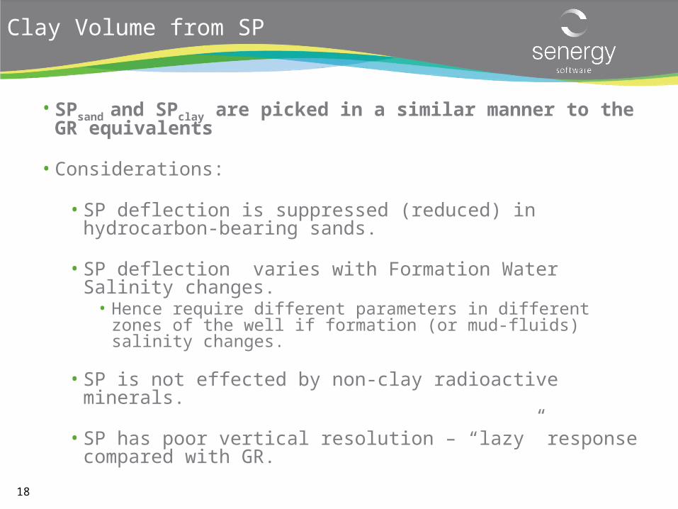
Clay Volume from SP

• SPsand and SPclay are picked in a similar manner to the GR equivalents

• Considerations:

• SP deflection is suppressed (reduced) in hydrocarbon-bearing sands.

• SP deflection varies with Formation Water Salinity changes.• Hence require different parameters in different zones of the well if

formation (or mud-fluids) salinity changes.

• SP is not effected by non-clay radioactive minerals.

• SP has poor vertical resolution – “lazy” response compared with GR.

19

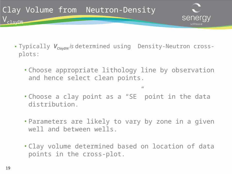
Clay Volume from Neutron-Density VclayDN

• Typically VClayDN is determined using Density-Neutron cross-plots:

• Choose appropriate lithology line by observation and hence select clean points.

• Choose a clay point as a “SE” point in the data distribution.

• Parameters are likely to vary by zone in a given well and between wells.

• Clay volume determined based on location of data points in the cross-plot.

20

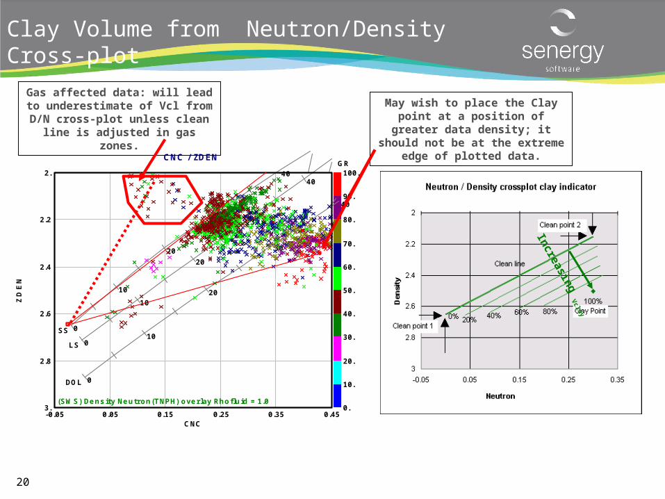
Clay Volume from Neutron/Density Cross-plot

Clay Point

Increasing V

clay

Callenish 1CNC / ZDEN

3.

2.8

2.6

2.4

2.2

2.

ZD

EN

-0.05 0.05 0.15 0.25 0.35 0.45CNC

0.

10.

20.

30.

40.

50.

60.

70.

80.

90.

100.GR

SS 0

10

20

30

40

LS 0

10

20

30

40

DOL 0

10

20

30

40

(SWS) Density Neutron(TNPH) overlay Rhofluid = 1.0

Gas affected data: will lead to underestimate of Vcl from D/N cross-plot unless clean line is

adjusted in gas zones.

May wish to place the Clay point at a position of greater data density; it should not be at the extreme edge

of plotted data.

21

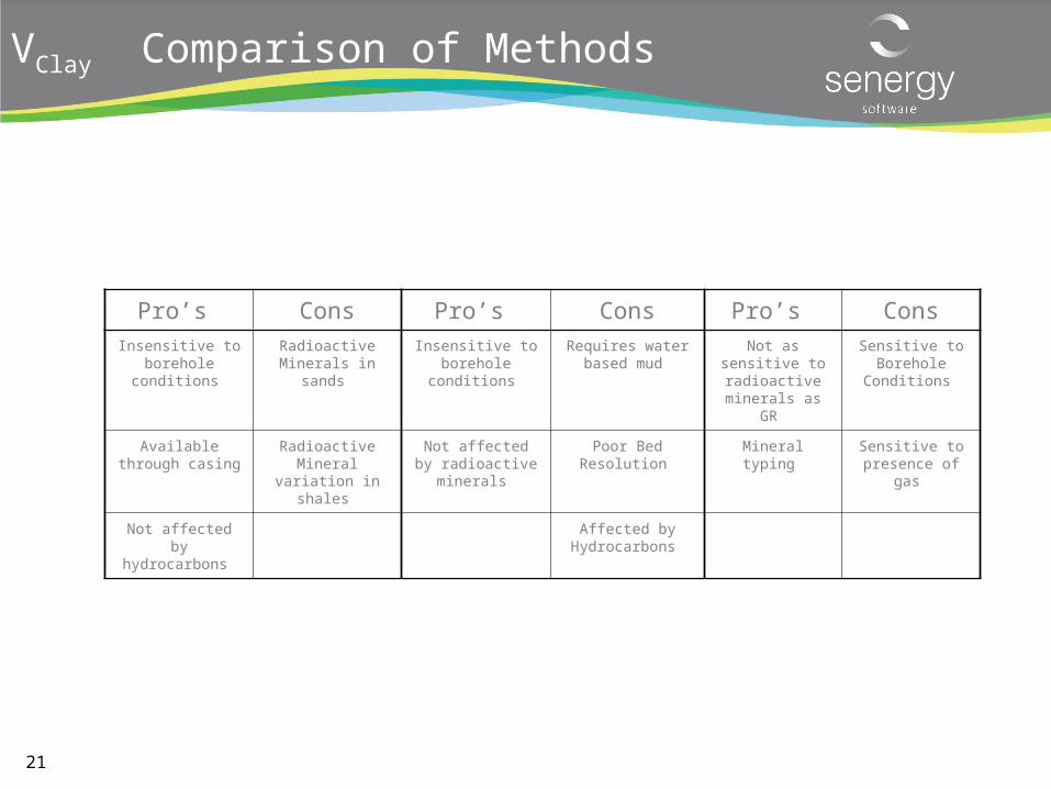
VClay Comparison of Methods

Pro’s Cons Pro’s Cons Pro’s ConsInsensitive to

borehole conditions

Radioactive Minerals in sands

Insensitive to borehole

conditions

Requires water based mud

Not as sensitive to radioactive

minerals as GR

Sensitive to Borehole

Conditions

Available through casing

Radioactive Mineral variation in

shales

Not affected by radioactive minerals

Poor Bed Resolution

Mineral typing Sensitive to presence of gas

Not affected by hydrocarbons

Affected by Hydrocarbons

www.senergyworld.com

Clay Volume Calculation in IP

23

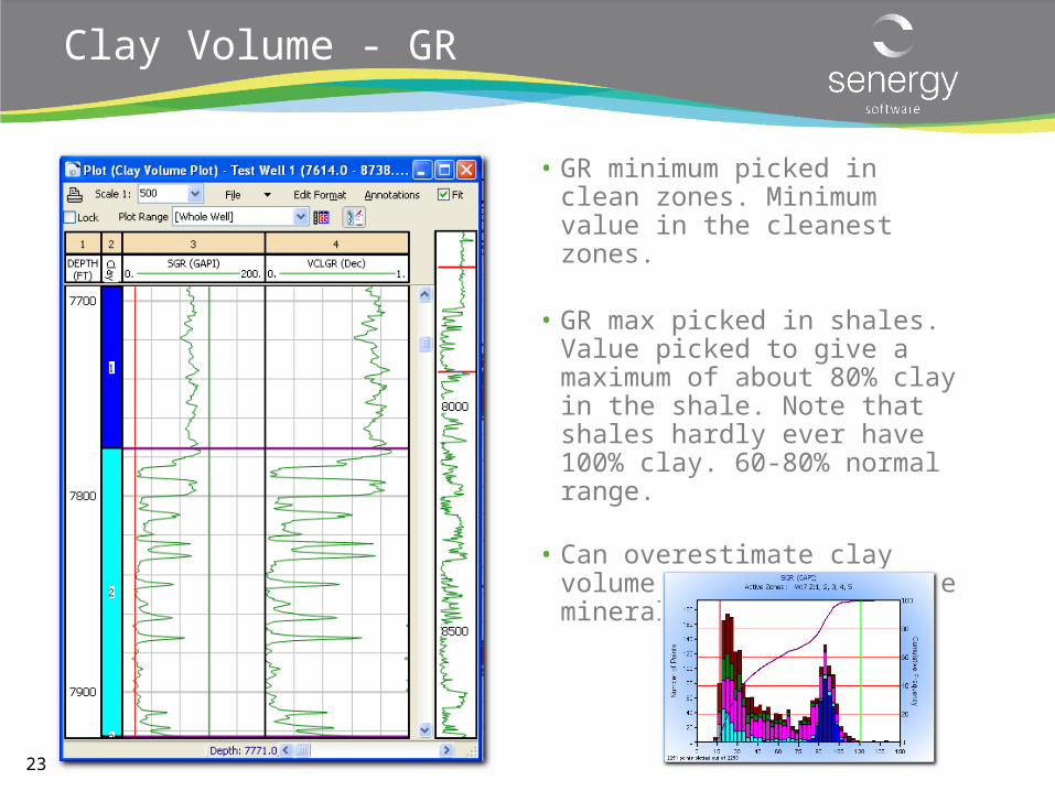
Clay Volume - GR

• GR minimum picked in clean zones. Minimum value in the cleanest zones.

• GR max picked in shales. Value picked to give a maximum of about 80% clay in the shale. Note that shales hardly ever have 100% clay. 60-80% normal range.

• Can overestimate clay volume due to radioactive minerals in the sands

24

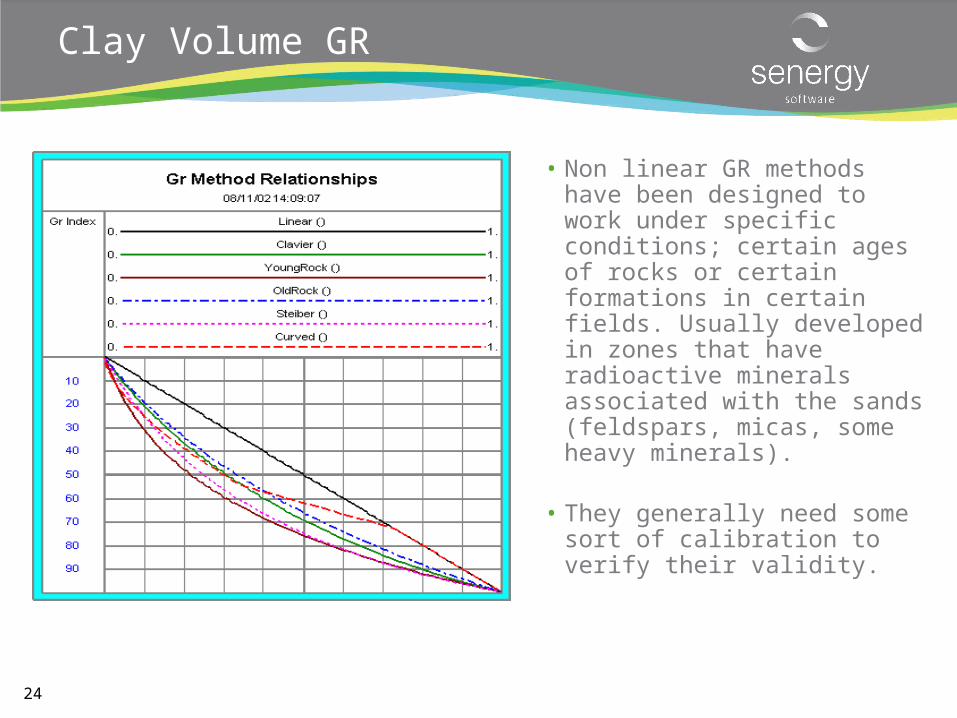
Clay Volume GR

• Non linear GR methods have been designed to work under specific conditions; certain ages of rocks or certain formations in certain fields. Usually developed in zones that have radioactive minerals associated with the sands (feldspars, micas, some heavy minerals).

• They generally need some sort of calibration to verify their validity.

25

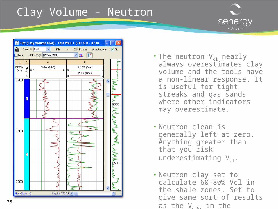
Clay Volume - Neutron

• The neutron Vcl nearly always overestimates clay volume and the tools have a non-linear response. It is useful for tight streaks and gas sands where other indicators may overestimate.

• Neutron clean is generally left at zero. Anything greater than that you risk underestimating Vcl.

• Neutron clay set to calculate 60-80% Vcl in the shale zones. Set to give same sort of results as the VclGR in the shales.

26

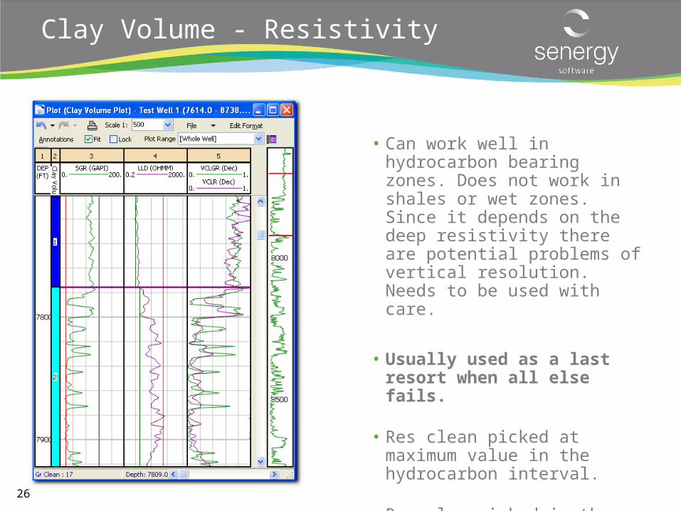
Clay Volume - Resistivity

• Can work well in hydrocarbon bearing zones. Does not work in shales or wet zones. Since it depends on the deep resistivity there are potential problems of vertical resolution. Needs to be used with care.

• Usually used as a last resort when all else fails.

• Res clean picked at maximum value in the hydrocarbon interval.

• Res clay picked in the shale zones.

27

Clay Volume - SP

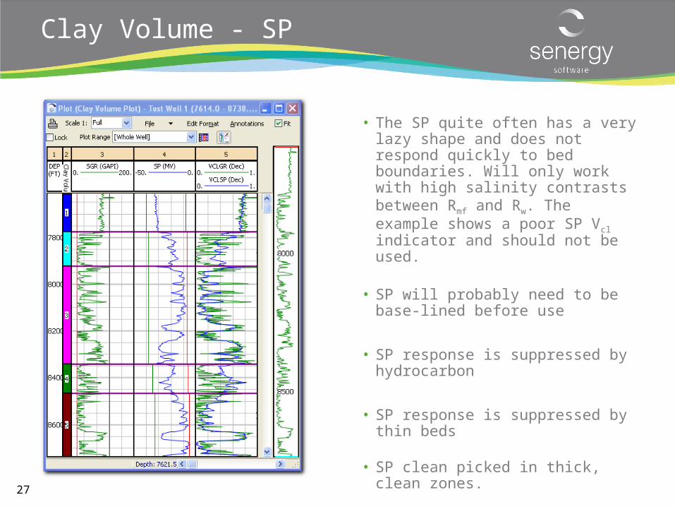
• The SP quite often has a very lazy shape and does not respond quickly to bed boundaries. Will only work with high salinity contrasts between Rmf and Rw. The example shows a poor SP Vcl indicator and should not be used.

• SP will probably need to be base-lined before use

• SP response is suppressed by hydrocarbon

• SP response is suppressed by thin beds

• SP clean picked in thick, clean zones.

• SP shale picked in the shales.

• Use with great care.

28

Clay Volume - Neutron Density

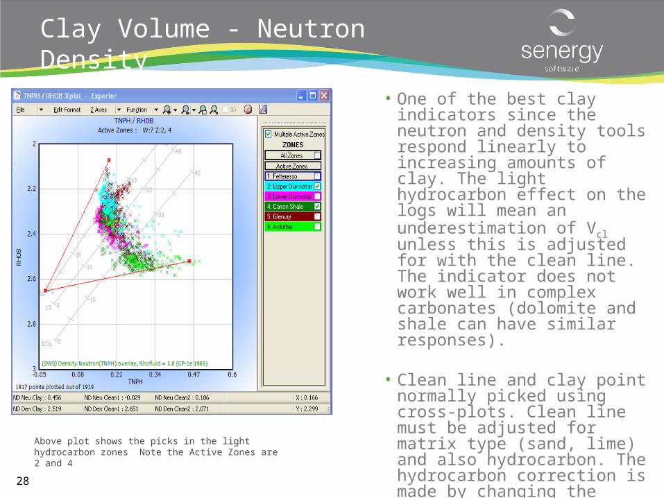
• One of the best clay indicators since the neutron and density tools respond linearly to increasing amounts of clay. The light hydrocarbon effect on the logs will mean an underestimation of Vcl unless this is adjusted for with the clean line. The indicator does not work well in complex carbonates (dolomite and shale can have similar responses).

• Clean line and clay point normally picked using cross-plots. Clean line must be adjusted for matrix type (sand, lime) and also hydrocarbon. The hydrocarbon correction is made by changing the slope on the clean matrix line.

• The Clay point is normally picked so that the N/D Vcl gives about 60-80% clay in the shales.

Above plot shows the picks in the light hydrocarbon zones Note the Active Zones are 2 and 4

29

Clay Volume - Sonic Density

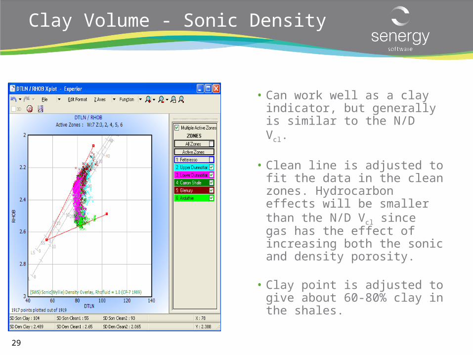
• Can work well as a clay indicator, but generally is similar to the N/D Vcl.

• Clean line is adjusted to fit the data in the clean zones. Hydrocarbon effects will be smaller than the N/D Vcl since gas has the effect of increasing both the sonic and density porosity.

• Clay point is adjusted to give about 60-80% clay in the shales.

30

Clay Volume - Sonic Neutron

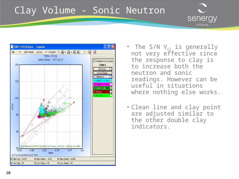
• The S/N Vcl is generally not very effective since the response to clay is to increase both the neutron and sonic readings. However can be useful in situations where nothing else works.

• Clean line and clay point are adjusted similar to the other double clay indicators.

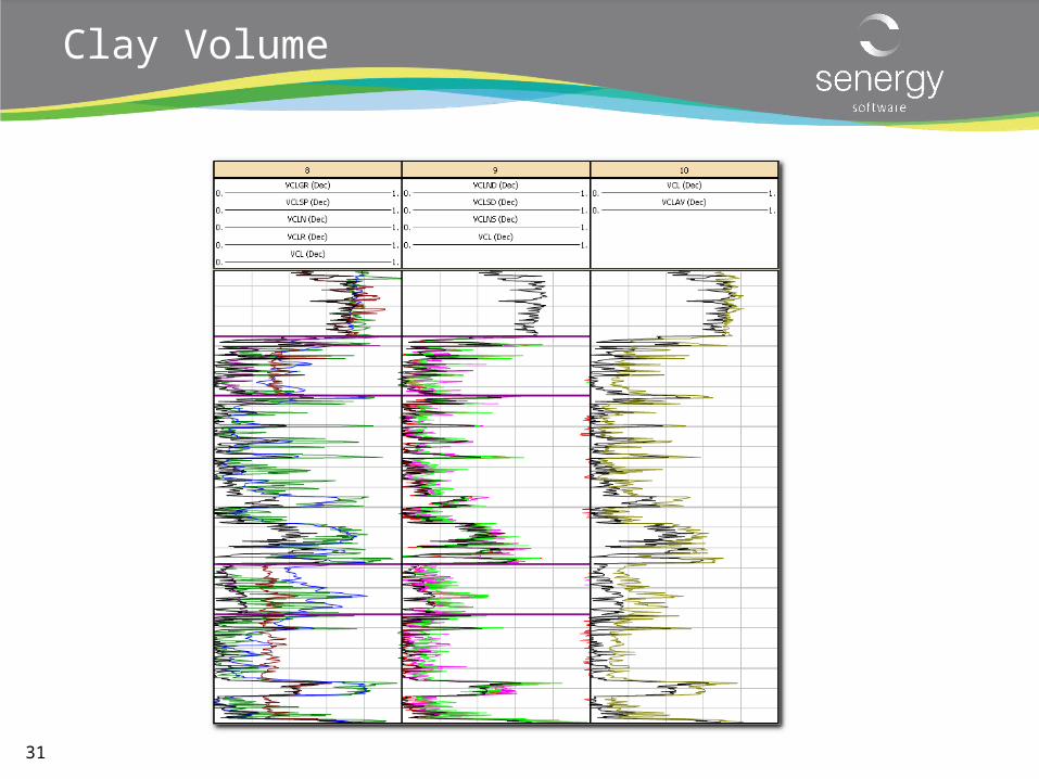
31

Clay Volume

www.senergyworld.com

Deterministic Petrophysics:Porosity

33

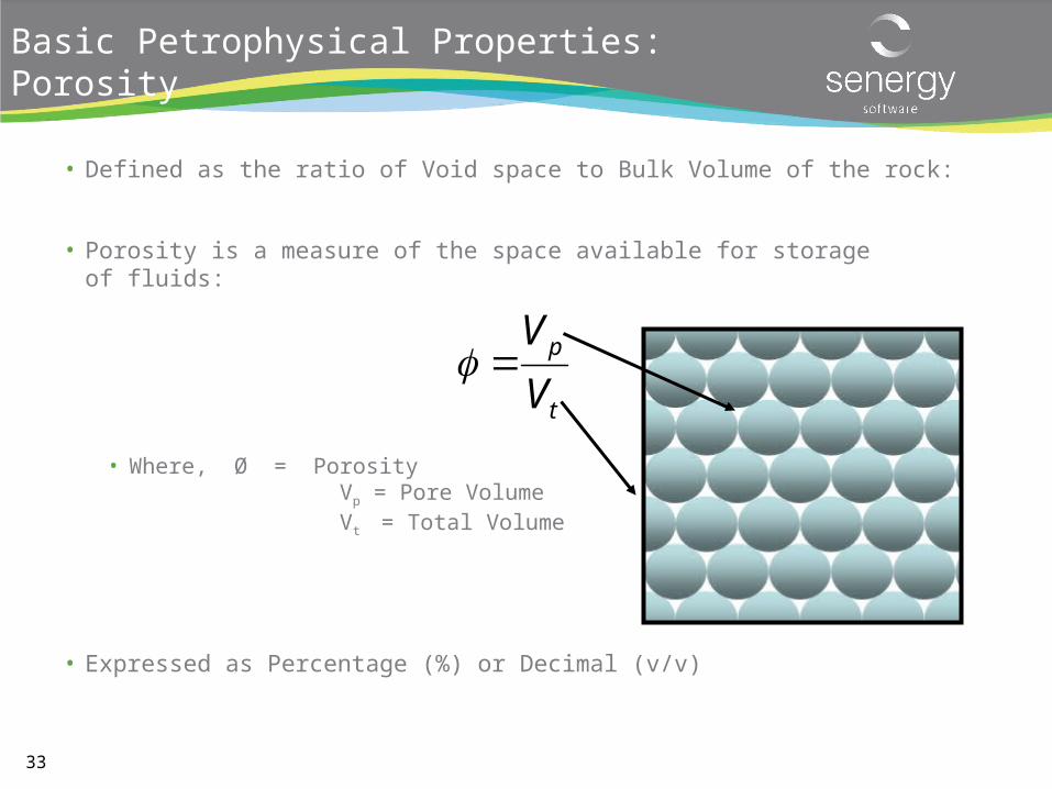
Basic Petrophysical Properties: Porosity

• Defined as the ratio of Void space to Bulk Volume of the rock:

• Porosity is a measure of the space available for storageof fluids:

• Where, Ø = PorosityVp = Pore VolumeVt = Total Volume

• Expressed as Percentage (%) or Decimal (v/v)

t

p

V

V

34

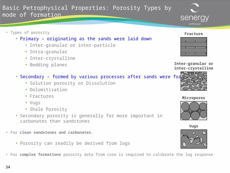
Basic Petrophysical Properties: Porosity Types by mode of formation

• Types of porosity

• Primary – originating as the sands were laid down

• Inter-granular or inter-particle

• Intra-granular

• Inter-crystalline

• Bedding planes

• Secondary – formed by various processes after sands were formed

• Solution porosity or Dissolution

• Dolomitisation

• Fractures

• Vugs

• Shale Porosity

• Secondary porosity is generally far more important in carbonates than sandstones

• For clean sandstones and carbonates,

• Porosity can readily be derived from logs

• For complex formations porosity data from core is required to calibrate the log response

Fracture

Vugs

Micropores

Inter-granular or inter-crystalline pores

35

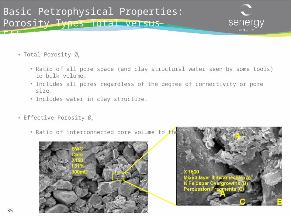
Basic Petrophysical Properties: Porosity Types Total versus Effective

• Total Porosity Øt

• Ratio of all pore space (and clay structural water seen by some tools) to bulk volume.

• Includes all pores regardless of the degree of connectivity or pore size.

• Includes water in clay structure.

• Effective Porosity Øe

• Ratio of interconnected pore volume to the bulk volume.

36

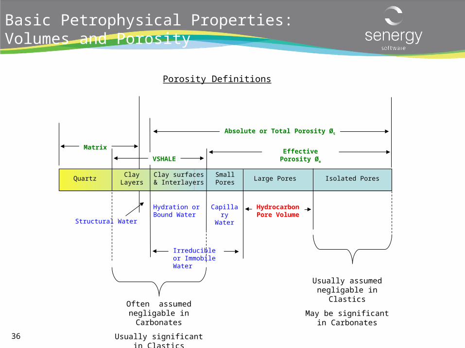
Basic Petrophysical Properties: Volumes and Porosity

Often assumed negligable in Carbonates

Usually significant in Clastics

Porosity Definitions

QuartzClay

LayersClay surfaces &

InterlayersSmall Pores

Large Pores Isolated Pores

Irreducible or Immobile Water

Structural Water

Hydrocarbon Pore Volume

Capillary Water

Hydration or Bound Water

Absolute or Total Porosity Øt

VSHALE

MatrixEffective Porosity Øe

Usually assumed negligable in Clastics

May be significant in Carbonates

37

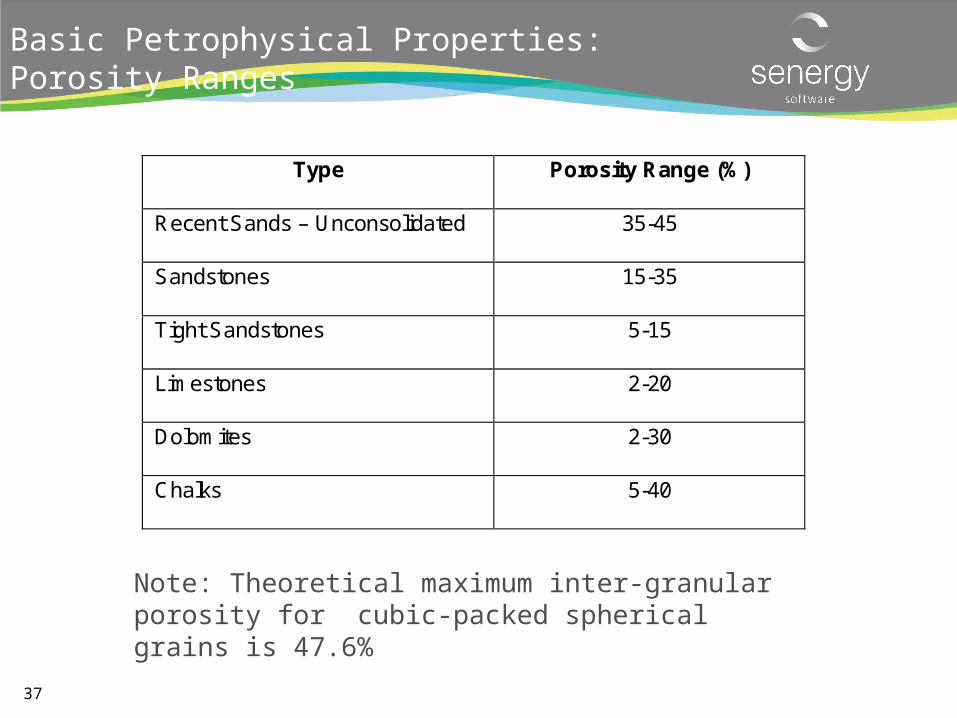
Basic Petrophysical Properties: Porosity Ranges

Type Porosity Range (%)

Recent Sands – Unconsolidated 35-45

Sandstones 15-35

Tight Sandstones 5-15

Limestones 2-20

Dolomites 2-30

Chalks 5-40

Note: Theoretical maximum inter-granular porosity for cubic-packed spherical grains is 47.6%

38

Basic Petrophysical Properties: Porosity measurements

• Core porosity

• Measure two of: pore volume, grain volume and bulk volume of core plug and ratio them.

• Direct measurement but:• Measure Øt or Øe (or something in between) depending on pore types present,

clay content and method of cleaning and drying.

• Measured under laboratory conditions rather than reservoir stress. Require correction to reservoir conditions for comparison with or calibration of log porosity.

• Log Porosity

• Sonic, Density, Density/Neutron, NMR.• Porosities measured differ.• No log measures porosity directly.• Calibrate to core when possible.

39

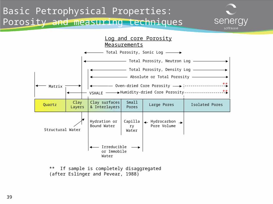
Basic Petrophysical Properties: Porosity and measuring techniques

Log and core Porosity Measurements

** If sample is completely disaggregated(after Eslinger and Pevear, 1988)

QuartzClay

LayersClay surfaces &

InterlayersSmall Pores

Large Pores Isolated Pores

Irreducible or Immobile Water

Structural Water

Hydrocarbon Pore Volume

Capillary Water

Hydration or Bound Water

Total Porosity, Neutron Log

Total Porosity, Density Log

Oven-dried Core Porosity

Humidity-dried Core Porosity

Absolute or Total Porosity

VSHALE

Matrix **

**

Total Porosity, Sonic Log

40

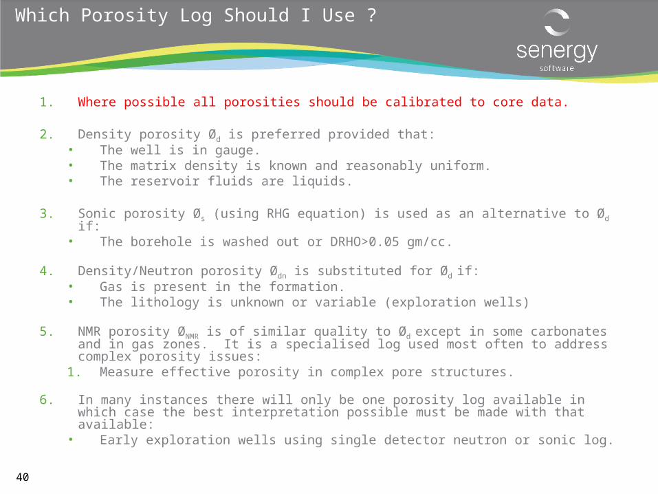
Which Porosity Log Should I Use ?

1. Where possible all porosities should be calibrated to core data.

2. Density porosity Ød is preferred provided that:• The well is in gauge. • The matrix density is known and reasonably uniform. • The reservoir fluids are liquids.

3. Sonic porosity Øs (using RHG equation) is used as an alternative to Ød if:• The borehole is washed out or DRHO>0.05 gm/cc.

4. Density/Neutron porosity Ødn is substituted for Ød if:• Gas is present in the formation.• The lithology is unknown or variable (exploration wells)

5. NMR porosity ØNMR is of similar quality to Ød except in some carbonates and in gas zones. It is a specialised log used most often to address complex porosity issues:

1. Measure effective porosity in complex pore structures.

6. In many instances there will only be one porosity log available in which case the best interpretation possible must be made with that available:

• Early exploration wells using single detector neutron or sonic log.

41

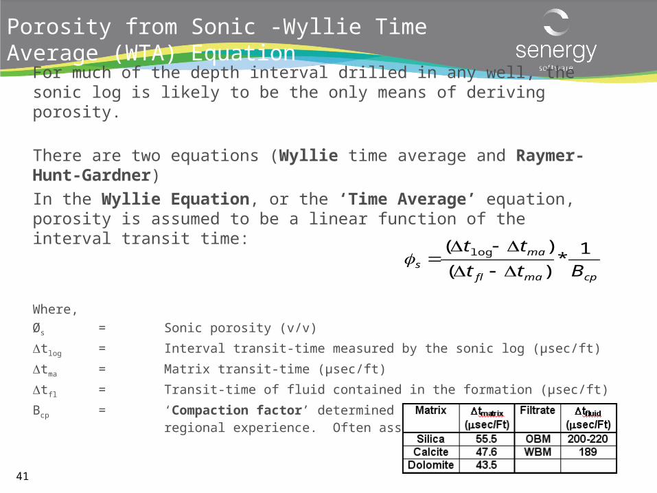
Porosity from Sonic -Wyllie Time Average (WTA) Equation

41

For much of the depth interval drilled in any well, the sonic log is likely to be the only means of deriving porosity.

There are two equations (Wyllie time average and Raymer-Hunt-Gardner) In the Wyllie Equation, or the ‘Time Average’ equation, porosity is assumed to be a linear function of the interval transit time:

Where,Øs = Sonic porosity (v/v)

tlog = Interval transit-time measured by the sonic log (μsec/ft)

tma = Matrix transit-time (μsec/ft)

tfl = Transit-time of fluid contained in the formation (μsec/ft)

Bcp = ‘Compaction factor’ determined by comparison with core or regional experience. Often assumed to be 1.

cpmafl

mas Btt

tt 1*

)(

)( log

42

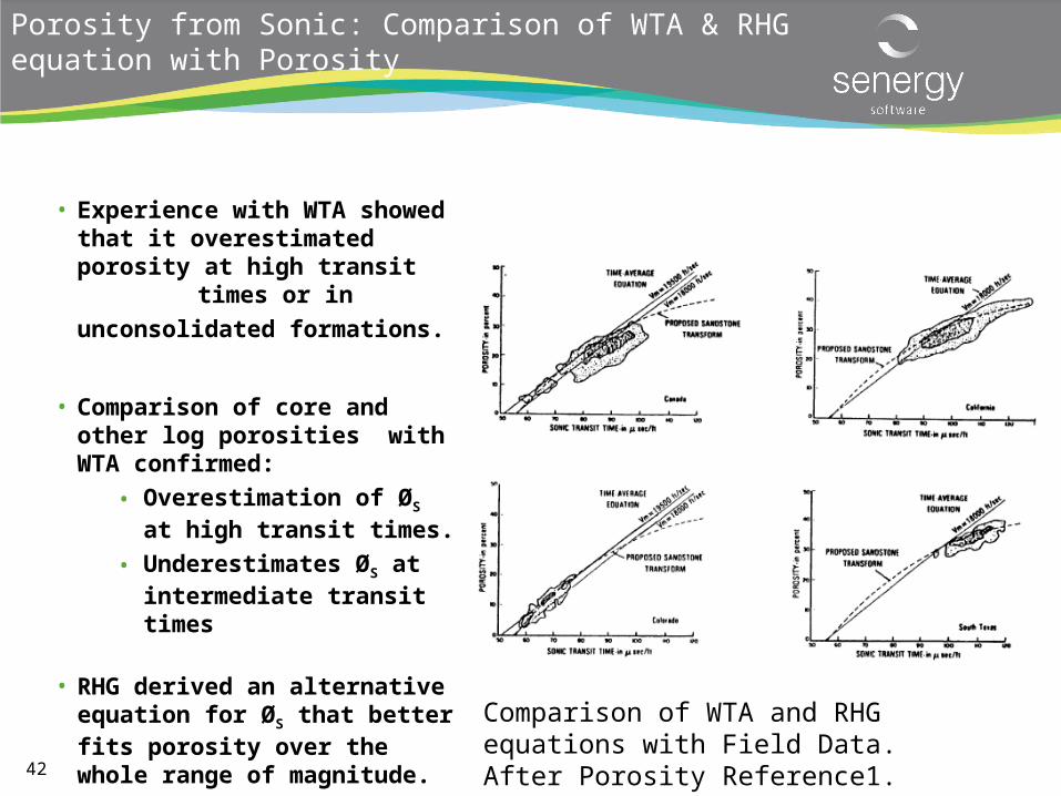
Comparison of WTA and RHG equations with Field Data. After Porosity Reference1.

Porosity from Sonic: Comparison of WTA & RHG equation with Porosity

• Experience with WTA showed that it overestimated porosity at high transit times or in

unconsolidated formations.

• Comparison of core and other log porosities with WTA confirmed:

• Overestimation of ØS at high transit times.

• Underestimates ØS at intermediate transit times

• RHG derived an alternative equation for ØS that better fits porosity over the whole range of magnitude.

43

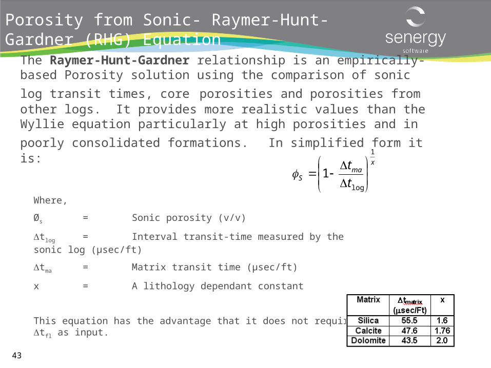
Porosity from Sonic- Raymer-Hunt-Gardner (RHG) Equation

The Raymer-Hunt-Gardner relationship is an empirically-based Porosity solution using the comparison of sonic log transit times,

core porosities and porosities from other logs. It provides more realistic values than the Wyllie equation particularly at high

porosities and in poorly consolidated formations. In simplified form it is:

Where,

Øs = Sonic porosity (v/v)

tlog = Interval transit-time measured by the sonic log (μsec/ft)

tma = Matrix transit time (μsec/ft)

x = A lithology dependant constant

This equation has the advantage that it does not require tfl as input.

xma

S t

t1

log

1

44

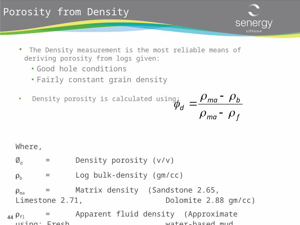
Porosity from Density

• The Density measurement is the most reliable means of deriving porosity from logs given:

• Good hole conditions

• Fairly constant grain density

• Density porosity is calculated using:

Where,

Ød = Density porosity (v/v)

b = Log bulk-density (gm/cc)

ma = Matrix density (Sandstone 2.65, Limestone 2.71, Dolomite 2.88 gm/cc)

fl = Apparent fluid density (Approximate using: Fresh water-based mud 1gm/cc, oil-based mud 0.85 gm/cc)

fma

bmad

45

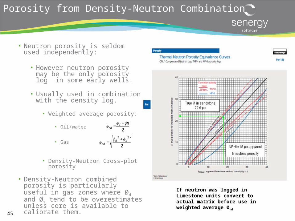
• Neutron porosity is seldom used independently:

• However neutron porosity may be the only porosity log in some early wells.

• Usually used in combination with the density log.

• Weighted average porosity:

• Oil/water

• Gas

• Density-Neutron Cross-plot porosity

• Density-Neutron combined porosity is particularly useful in gas zones where Ød and Øs tend to be overestimates unless core is available to calibrate them.

Porosity from Density-Neutron Combination

2

ndnd

2

`22nd

nd

If neutron was logged in Limestone units convert to actual matrix before use in weighted average Ønd

46

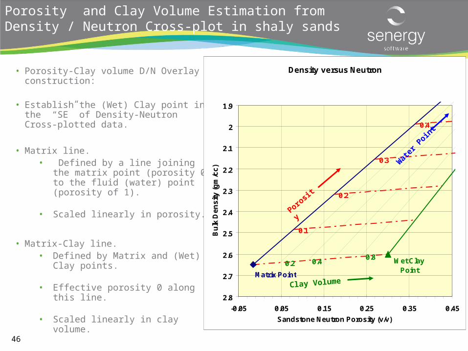
Porosity and Clay Volume Estimation from Density / Neutron Cross-plot in shaly sands

• Porosity-Clay volume D/N Overlay construction:

• Establish the (Wet) Clay point in the “SE” of Density-Neutron Cross-plotted data.

• Matrix line.• Defined by a line joining the matrix

point (porosity 0) to the fluid (water) point (porosity of 1).

• Scaled linearly in porosity.

• Matrix-Clay line.

• Defined by Matrix and (Wet) Clay points.

• Effective porosity 0 along this line.

• Scaled linearly in clay volume.

46

Density versus Neutron

0.2

0.3

0.4

0.2 0.40.8

Matrix Point

Wet Clay Point

0.1

1.9

2

2.1

2.2

2.3

2.4

2.5

2.6

2.7

2.8

-0.05 0.05 0.15 0.25 0.35 0.45

Sandstone Neutron Porosity (v/v)

Bu

lk D

en

sit

y (

gm

/cc

)

Clay Volume

Porosity

Wat

er P

oint

47

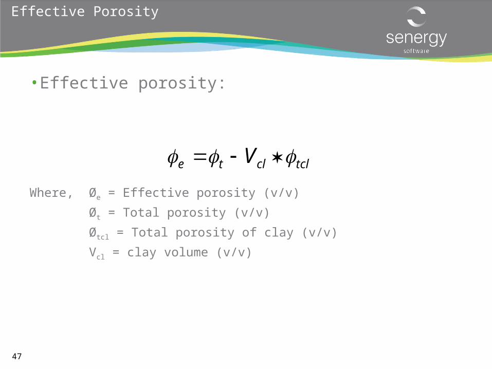
Effective Porosity

• Effective porosity:

Where, Øe = Effective porosity (v/v)

Øt = Total porosity (v/v)

Øtcl = Total porosity of clay (v/v)

Vcl = clay volume (v/v)

tclclte V

48

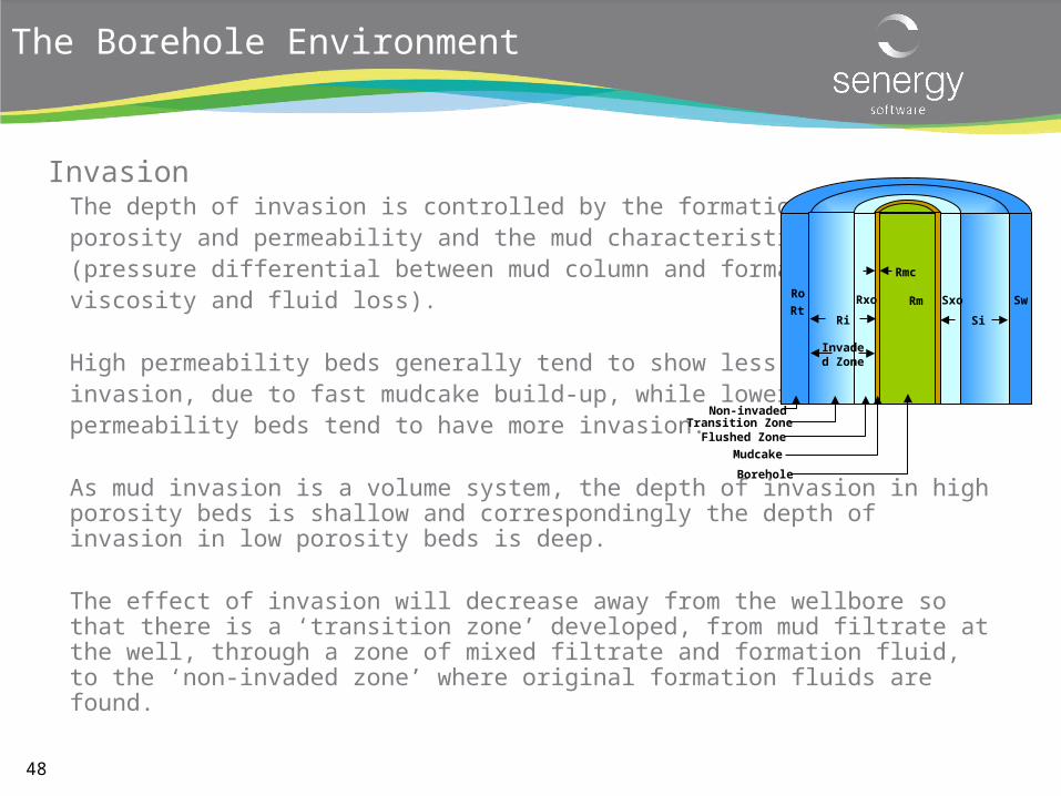
The Borehole Environment

InvasionThe depth of invasion is controlled by the formation porosity and permeability and the mud characteristics (pressure differential between mud column and formation, viscosity and fluid loss).

High permeability beds generally tend to show less invasion, due to fast mudcake build-up, while lower permeability beds tend to have more invasion.

As mud invasion is a volume system, the depth of invasion in high porosity beds is shallow and correspondingly the depth of invasion in low porosity beds is deep.

The effect of invasion will decrease away from the wellbore so that there is a ‘transition zone’ developed, from mud filtrate at the well, through a zone of mixed filtrate and formation fluid, to the ‘non-invaded zone’ where original formation fluids are found.

Ro

Rmc

RtRm Sw

Invaded Zone

Ri Si

Transition Zone

Mudcake

Flushed Zone

Non-invaded

Borehole

SxoRxo

49

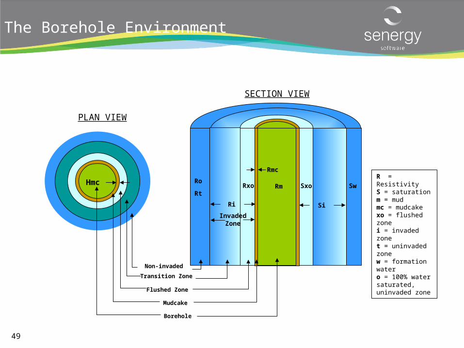
The Borehole Environment

R = ResistivityS = saturationm = mudmc = mudcakexo = flushed zonei = invaded zonet = uninvaded zonew = formation watero = 100% water saturated, uninvaded zone

Hmc RoRxo

Rmc

RtRm Sxo Sw

Invaded Zone

Ri Si

Transition Zone

Mudcake

Flushed Zone

Non-invaded

Borehole

PLAN VIEW

SECTION VIEW

50

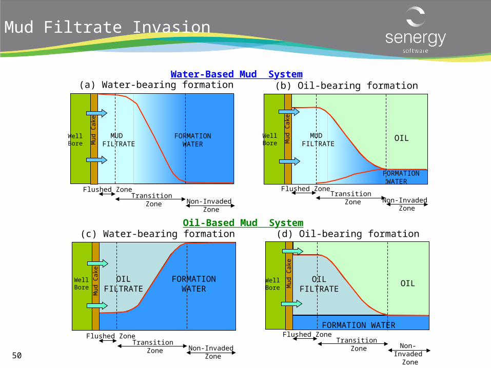
Mud Filtrate Invasion

Oil-Based Mud System(c) Water-bearing formation (d) Oil-bearing formation

FORMATIONWATER

OILFILTRATE

Well Bore

Mu

d C

ake

Flushed ZoneTransition

Zone Non-Invaded Zone

Water-Based Mud System

FORMATION WATER

MUD FILTRATE

(a) Water-bearing formation

MUD FILTRATE

FORMATIONWATER

Well Bore M

ud

Cak

e

Flushed ZoneTransition

Zone Non-Invaded Zone

OIL

FORMATION WATER

MUD FILTRATE

(b) Oil-bearing formation

Well Bore M

ud

Cak

e

Flushed ZoneTransition

Zone Non-Invaded Zone

OIL

FORMATION WATER

OILFILTRATE

Well Bore M

ud

Cak

e

Flushed ZoneTransition

Zone Non-Invaded Zone

51

Fluid Parameter Determination for Porosity Calculation

• All porosity calculations require a fluid parameter• Ød fluid density f

• Øs fluid transit time tf

• Øn fluid hydrogen index HIf

• It can be assumed that the porosity logs measure predominantly in the in the flushed zone.

• Hence the fluid parameter will be a weighted average of mud-filtrate, formation water and where present hydrocarbon properties dependent on the saturations of those fluids in the invaded zone.

• For this reason porosity and saturation calculations are linked in IP.

52

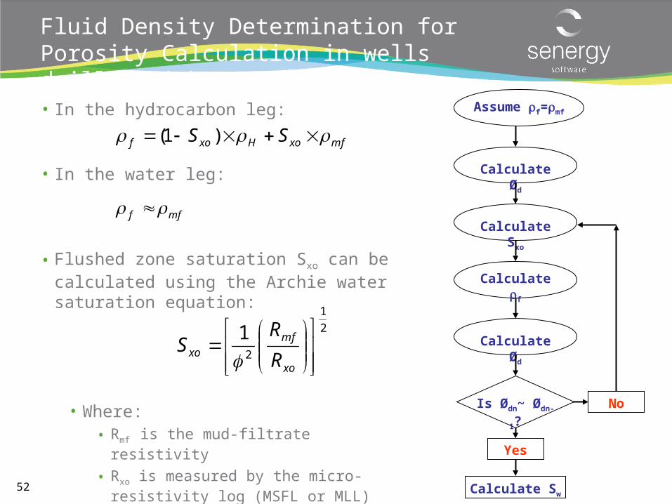
• In the hydrocarbon leg:

• In the water leg:

• Flushed zone saturation Sxo can be calculated using the Archie water saturation equation:

• Where:• Rmf is the mud-filtrate resistivity

• Rxo is measured by the micro-resistivity log (MSFL or MLL)

• Ø is the porosity

Fluid Density Determination for Porosity Calculation in wells drilled with WBM

mfxoHxof SS )1(

mff

2

1

2

1

xo

mfxo R

RS

Assume f=mf

Calculate Ød

Calculate Sxo

Calculate f

Calculate Ød

Is Ødn~ Ødn-1?

Yes

No

Calculate Sw

53

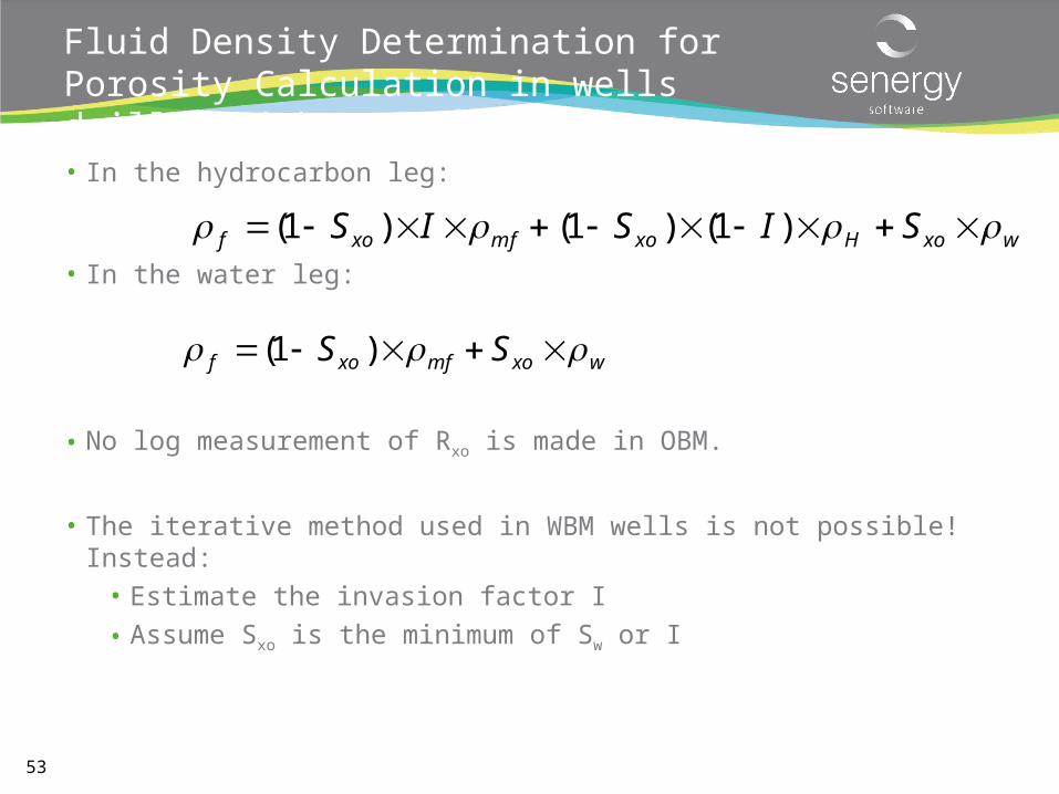
Fluid Density Determination for Porosity Calculation in wells drilled with OBM

• In the hydrocarbon leg:

• In the water leg:

• No log measurement of Rxo is made in OBM.

• The iterative method used in WBM wells is not possible!Instead:

• Estimate the invasion factor I

• Assume Sxo is the minimum of Sw or I

wxomfxof SS )1(

wxoHxomfxof SISIS )1()1()1(

www.senergyworld.com

Porosity Calculation in IP

55

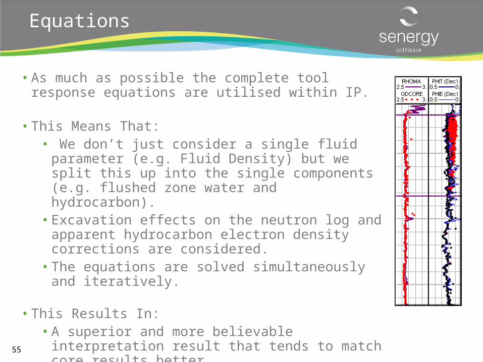
Equations

• As much as possible the complete tool response equations are utilised within IP.

• This Means That:• We don’t just consider a single fluid parameter (e.g.

Fluid Density) but we split this up into the single components (e.g. flushed zone water and hydrocarbon).

• Excavation effects on the neutron log and apparent hydrocarbon electron density corrections are considered.

• The equations are solved simultaneously and iteratively.

• This Results In:• A superior and more believable interpretation result that

tends to match core results better.

56

Equations

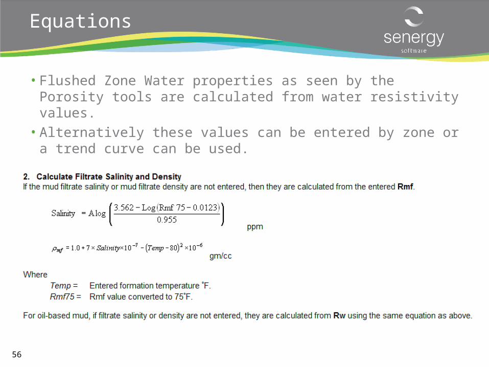
• Flushed Zone Water properties as seen by the Porosity tools are calculated from water resistivity values.

• Alternatively these values can be entered by zone or a trend curve can be used.

57

Equations

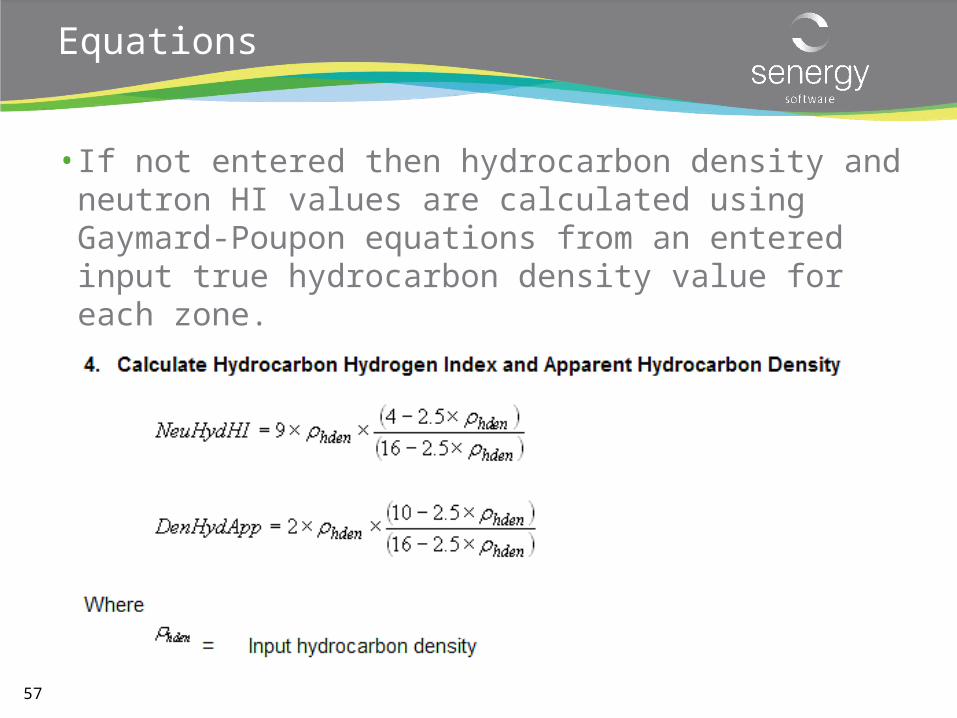
• If not entered then hydrocarbon density and neutron HI values are calculated using Gaymard-Poupon equations from an entered input true hydrocarbon density value for each zone.

58

Porosity Models - Density

59

Porosity Models - Density

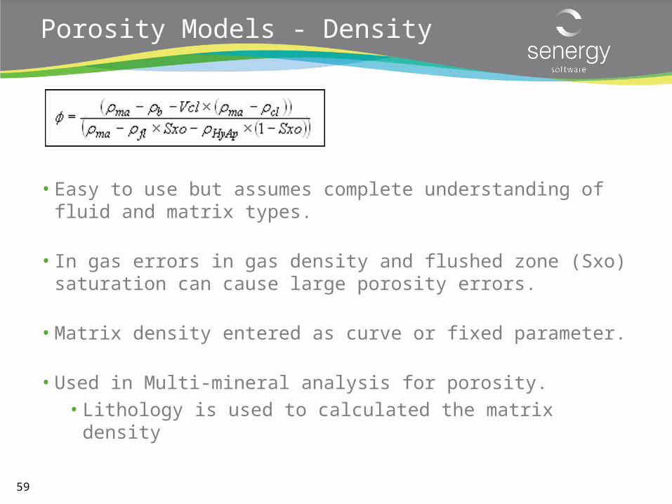
• Easy to use but assumes complete understanding of fluid and matrix types.

• In gas errors in gas density and flushed zone (Sxo) saturation can cause large porosity errors.

• Matrix density entered as curve or fixed parameter.

• Used in Multi-mineral analysis for porosity.• Lithology is used to calculated the matrix density

60

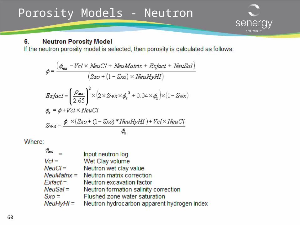
Porosity Models - Neutron

61

Porosity Models - Neutron

• Non linear response equation to minerals and hydrocarbons• Equations are tool specific• IP allows the selection of the tool type

• Tools are very sensitive to borehole corrections.

• Large gas correction required• Gas correction reverse of the density

• The neutron is rarely used by itself. Normal used in conjunction with the density to calculate a neutron / density porosity.

• To use non linear matrix enter Rho matrix for required mineral (2.65 for sand) otherwise enter the matrix neutron porosity

62

Porosity Models - Sonic

• Two empirical relationships in IP• Wyllie• Raymer Hunt

• Input parameters are hard to pin down and best set by calibrating to another porosity

• Gas effects can be large in high porosity• Hard to correct for

• Sonic used when• No density available• Density effected by hole washout• Unusual lithology where density matrix is not known

• Volcanics

63

Porosity Models – Neutron / Density

64

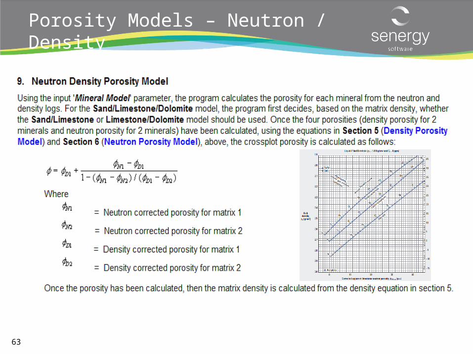
Porosity Models – Neutron / Density

• Preferred method in IP

• Two input equations so can calculated two outputs• Porosity + Hydrocarbon Density• Porosity + Matrix Density• Porosity + Clay Volume

• Three methods for controlling the logic• Calculate hydrocarbon density using a fixed matrix density• Calculate matrix density using a fixed hydrocarbon density• Calculate clay volume using a fixed hydrocarbon and matrix

density

65

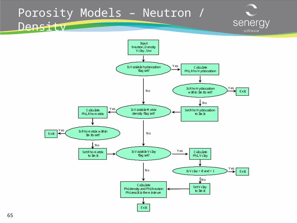
Porosity Models – Neutron / Density

Input Neutron, Density

Vclay, Sxo

Calculate Phi, Rho matrix

Is Variable hydrocarbon flag set?

Is Rho Hydrocarbon within limits set?

Is Variable Vclay flag set?

Calculate Phi, Rho Hydrocarbon

Is Rho matrix within limits set?

Is Variable Matrix density flag set?

Calculate Phi, Vclay

Is Vclay > 0 and < 1

Set Rho Hydrocarbon to limit

Set Rho matrix to limit

Exit

Exit

Exit

Set Vclay to limit

Calculate Phi density and Phi Neutron Phi result is the minimum

Exit

Yes

Yes

Yes

Yes

Yes

Yes

No

No

No

No

No

No

66

Porosity Models – Neutron / Sonic

• Used similar logic to Neutron / Density

• Rarely used since the N / D is more accurate and easier to understand and control

• Sonic parameter selection

67

Porosity and Water Saturation

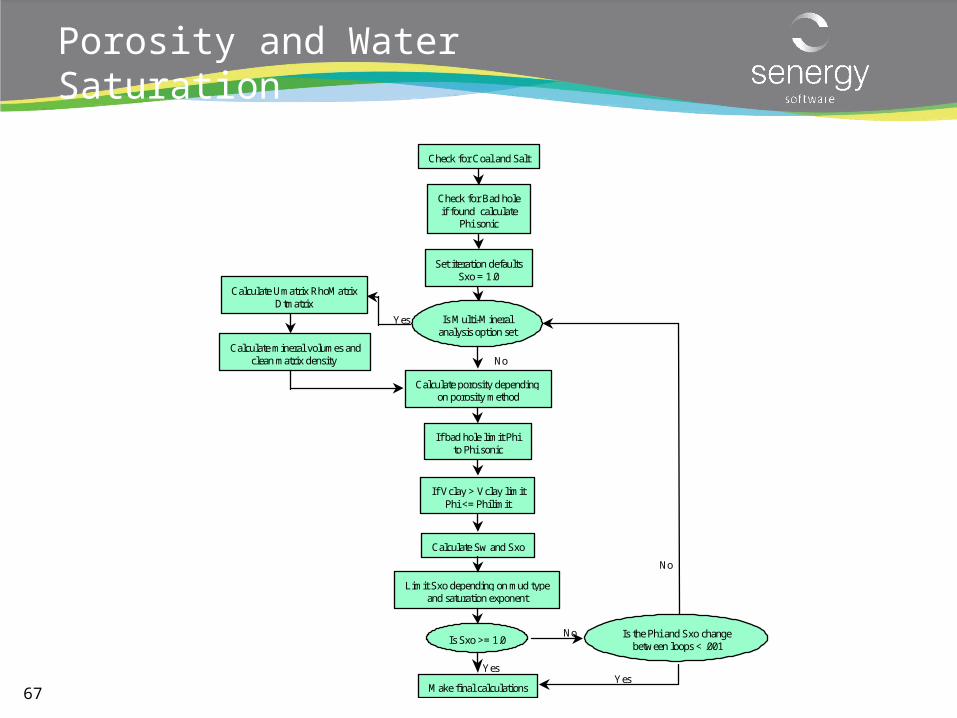
Check for Coal and Salt

Check for Bad holeif found calculate

Phi sonic

Set iteration defaultsSxo = 1.0

Calculate porosity dependingon porosity method

If bad hole limit Phito Phi sonic

Limit Sxo depending on mud typeand saturation exponent

Calculate Sw and Sxo

If Vclay > Vclay limitPhi <= Philimit

Is Sxo >= 1.0Is the Phi and Sxo change

between loops < .001

Make final calculations

No

YesYes

No

Is Multi-Mineralanalysis option set

Yes

Calculate Umatrix RhoMatrixDtmatrix

Calculate mineral volumes andclean matrix density No

68

Porosity Models – Pass through Porosity

• For users who want to calculated Phi outside the normal routine

• Regression against core data• NMR porosity

• Program needs to know if input porosity is a total or effective porosity

• All normal logic is applied• Sw calculations• Bad hole logic

www.senergyworld.com

Deterministic Petrophysics:Water Saturation

70

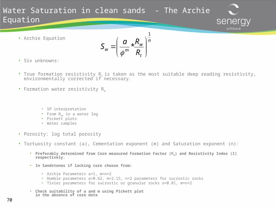
Water Saturation in clean sands - The Archie Equation

• Archie Equation

• Six unknowns:

• True formation resistivity Rt is taken as the most suitable deep reading resistivity, environmentally corrected if necessary.

• Formation water resistivity Rw

• SP interpretation• From Rwa in a water leg• Pickett plots• Water samples

• Porosity: log total porosity

• Tortuosity constant (a), Cementation exponent (m) and Saturation exponent (n):

• Preferably determined from Core measured Formation Factor (FR) and Resistivity Index (I) respectively.

• In Sandstones if lacking core choose from:

• Archie Parameters a=1, m=n=2• Humble parameters a=0.62, m=2.15, n=2 parameters for sucrostic rocks• Tixier parameters for sucrostic or granular rocks a=0.81, m=n=2

• Check suitability of a and m using Pickett plotin the absence of core data

n

t

wmw R

RaS

1

*

71

a.Rw

Slope m = 2

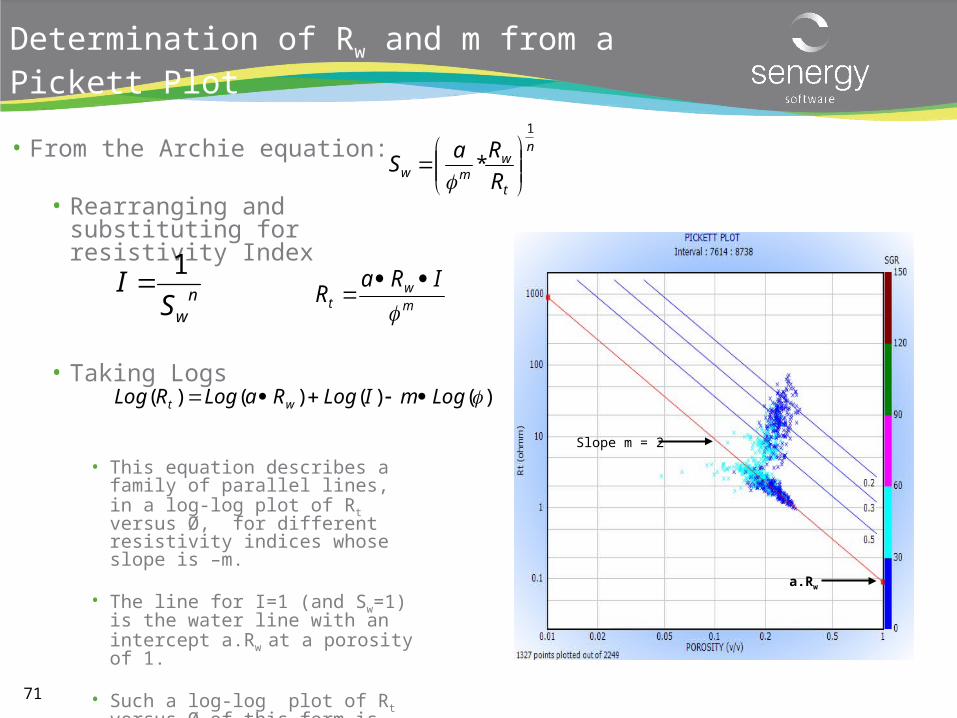
Determination of Rw and m from a Pickett Plot

• From the Archie equation:

• Rearranging and substituting for resistivity Index

• Taking Logs

• This equation describes a family of parallel lines, in a log-log plot of Rt versus Ø, for different resistivity indices whose slope is –m.

• The line for I=1 (and Sw=1) is the water line with an intercept a.Rw at a porosity of 1.

• Such a log-log plot of Rt versus Ø of this form is called a Pickett Plot.

n

t

wmw R

RaS

1

*

mw

t

IRaR

)()()()( LogmILogRaLogRLog wt

nwS

I1

72

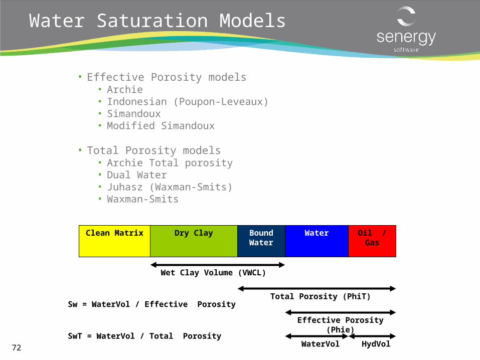
Water Saturation Models

• Effective Porosity models• Archie• Indonesian (Poupon-Leveaux)• Simandoux• Modified Simandoux

• Total Porosity models• Archie Total porosity• Dual Water• Juhasz (Waxman-Smits)• Waxman-Smits

Clean Matrix Dry Clay Bound Water

Water Oil / Gas

Total Porosity (PhiT)

Effective Porosity (Phie)

HydVolWaterVol

Sw = WaterVol / Effective Porosity

SwT = WaterVol / Total Porosity

Wet Clay Volume (VWCL)

73

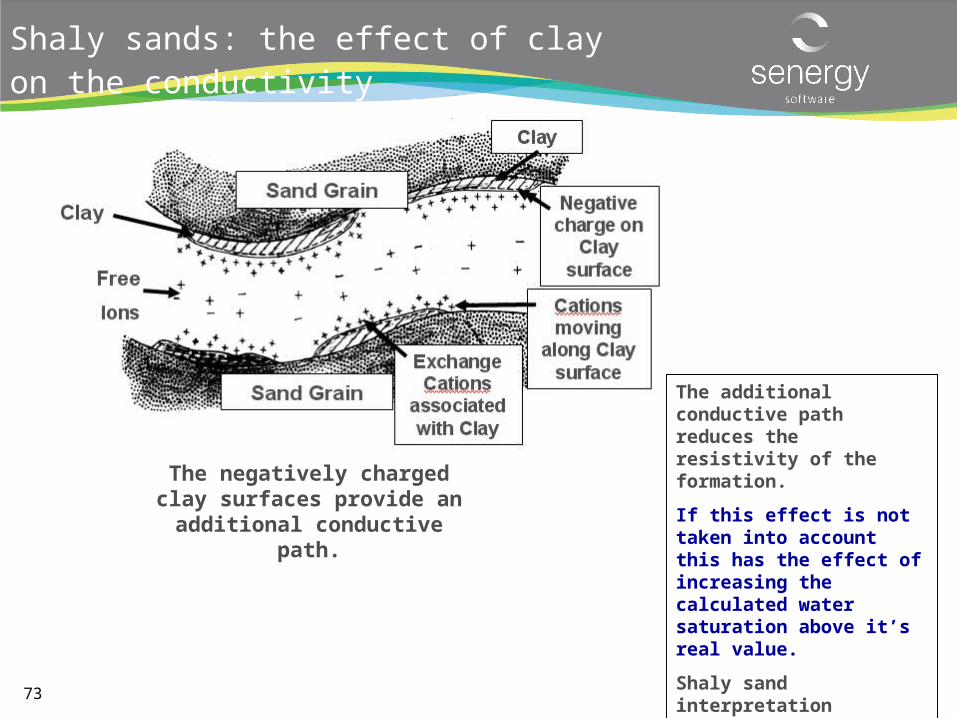
Shaly sands: the effect of clay on the conductivity

The negatively charged clay surfaces provide an additional

conductive path.

The additional conductive path reduces the resistivity of the formation.

If this effect is not taken into account this has the effect of increasing the calculated water saturation above it’s real value.

Shaly sand interpretation corrects for this effect to calculate Sw.

74

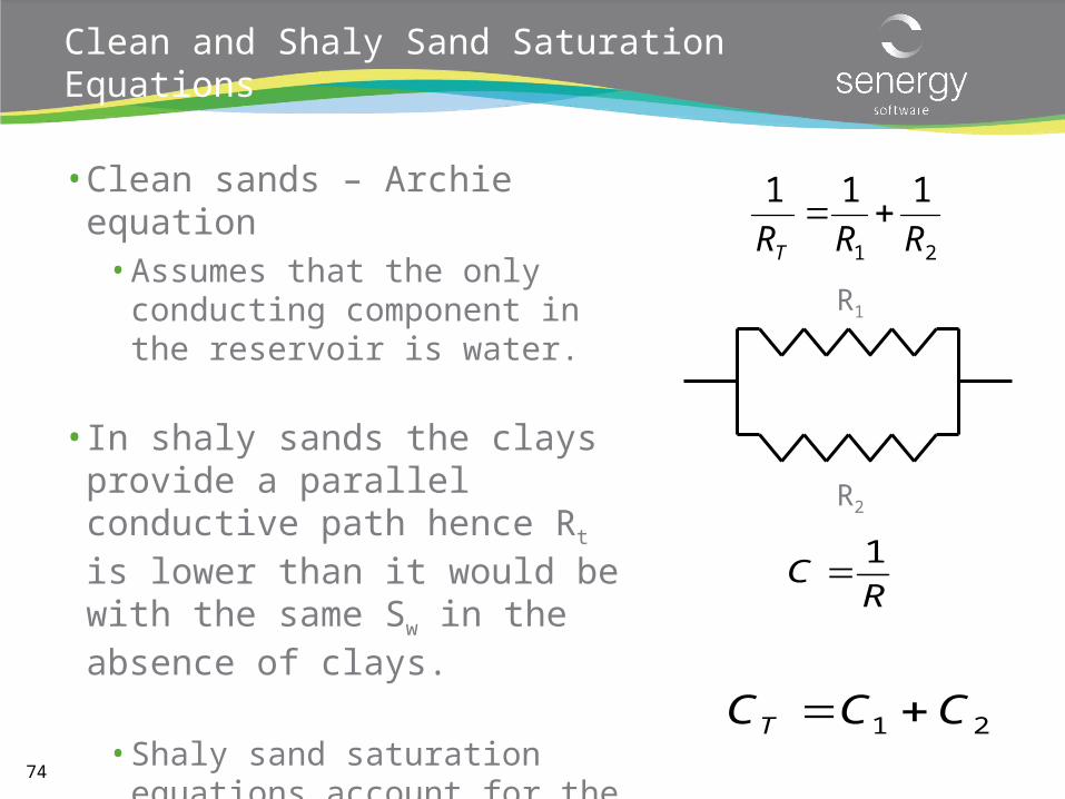
Clean and Shaly Sand Saturation Equations

• Clean sands – Archie equation• Assumes that the only conducting

component in the reservoir is water.

• In shaly sands the clays provide a parallel conductive path hence Rt is lower than it would be with the same Sw in the absence of clays.

• Shaly sand saturation equations account for the extra conductivity provided by the shales.

R1

R2

21

111

RRRT

RC

1

21 CCCT

75

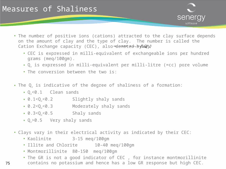
Measures of Shaliness

• The number of positive ions (cations) attracted to the clay surface depends on the amount of clay and the type of clay. The number is called the Cation Exchange capacity (CEC), also denoted by Qv.

• CEC is expressed in milli-equivalent of exchangeable ions per hundred grams (meq/100gm).

• Qv is expressed in milli-equivalent per milli-litre (=cc) pore volume

• The conversion between the two is:

• The Qv is indicative of the degree of shaliness of a formation:

• Qv<0.1 Clean sands

• 0.1<Qv<0.2Slightly shaly sands

• 0.2<Qv<0.3Moderately shaly sands

• 0.3<Qv<0.5Shaly sands

• Qv>0.5 Very shaly sands

• Clays vary in their electrical activity as indicated by their CEC:

• Kaolinite 3-15 meq/100gm

• Illite and Chlorite 10-40 meq/100gm

• Montmorillinite 80-150 meq/100gm

• The GR is not a good indicator of CEC , for instance montmorillinite contains no potassium and hence has a low GR response but high CEC.

t

tgv CECQ

100

)1(

76

Shaly sands

• The Archie equation assumes that the matrix is non-conducting.

• In shaly sands the resistivity is lower than in clean sands for the same Ø and Sw. This is caused by the additional electrical conductivity of the clay.

• Hence use of the Archie equation in shaly sands will result in too low a hydrocarbon saturation.

• There are a large number of shaly-sand Sw equations.

• All have the basic Archie form with an additional term to account for the extra conductivity of the clay.

• The clay-distributions for which the equations are intended are not always clear.

• Two equations will be described here:

• The Indonesia Equation – well adapted for application without supporting core analysis data.

• The Waxman-Smits equation – which is intended for application where the clays coat the matrix grains (dispersed shale). This equation performs well when core measurements of the clay properties are available.

77

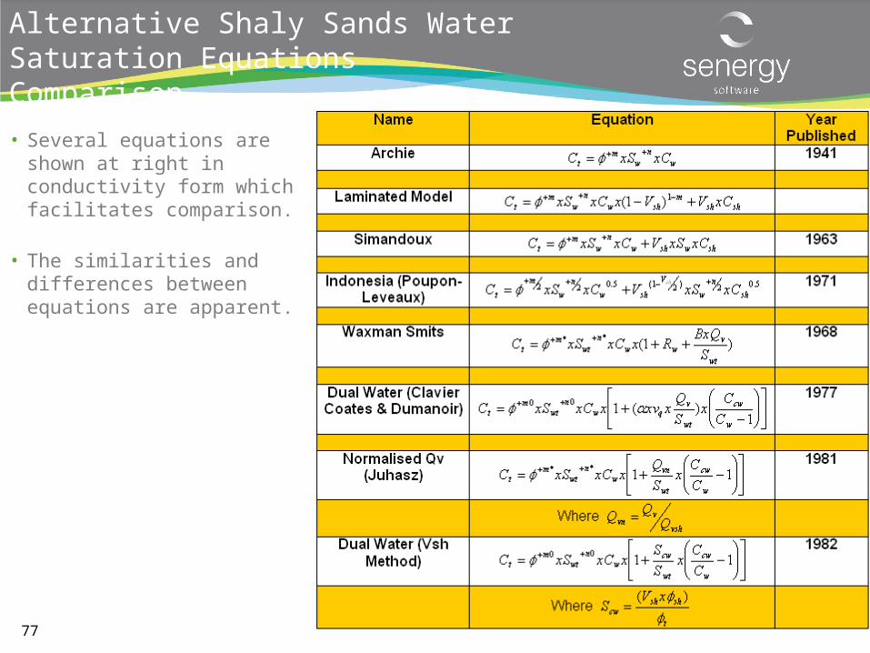
Alternative Shaly Sands Water Saturation EquationsComparison

• Several equations are shown at right in conductivity form which facilitates comparison.

• The similarities and differences between equations are apparent.

7777

78

When do I Need to use a Shaly Sand Interpretation?

• If possible treat sands as “clean” – non-shaly because it is much simpler to do so!• In that case Øt = Øe and the Archie equation can be used to determine Sw.

• How can you tell if you need to use a shaly sand approach or not?

• If the formation has high shale volumes as seen in core.

• If CEC or Qv measurements on core indicate high values.

• Compare wetting phase saturations from air-mercury and air-brine Pc data. If the latter are significantly larger than the former then the difference is due to clays (which do not influence air/mercury saturations) and the need for shaly sand interpretation is indicated.

• The fresher the formation water the more significant will be the effect of shale content. At high salinity (100’s of kppm) shale effects become negligible even with substantial clay content.

• Examine the formation resistivity in sands; if it shows a dependence on shale volume you need to use Shaly sand interpretation.

• If in doubt as to the significance of shales calculate Sw using the Archie equation and a simple shaly sand equation (suggest the Indonesia equation) and see how much difference the two approaches make to Sw (and Sh)

79

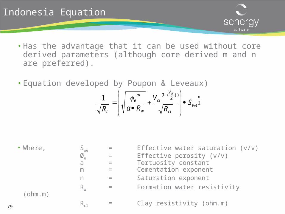
Indonesia Equation

• Has the advantage that it can be used without core derived parameters (although core derived m and n are preferred).

• Equation developed by Poupon & Leveaux)

• Where, Swe = Effective water saturation (v/v)Øe = Effective porosity (v/v)a = Tortuosity constantm = Cementation exponentn = Saturation exponent

Rw = Formation water resistivity (ohm.m)

Rcl = Clay resistivity (ohm.m)

2

))2

(1(1 n

we

cl

V

cl

w

me

t

SR

V

RaR

cl

80

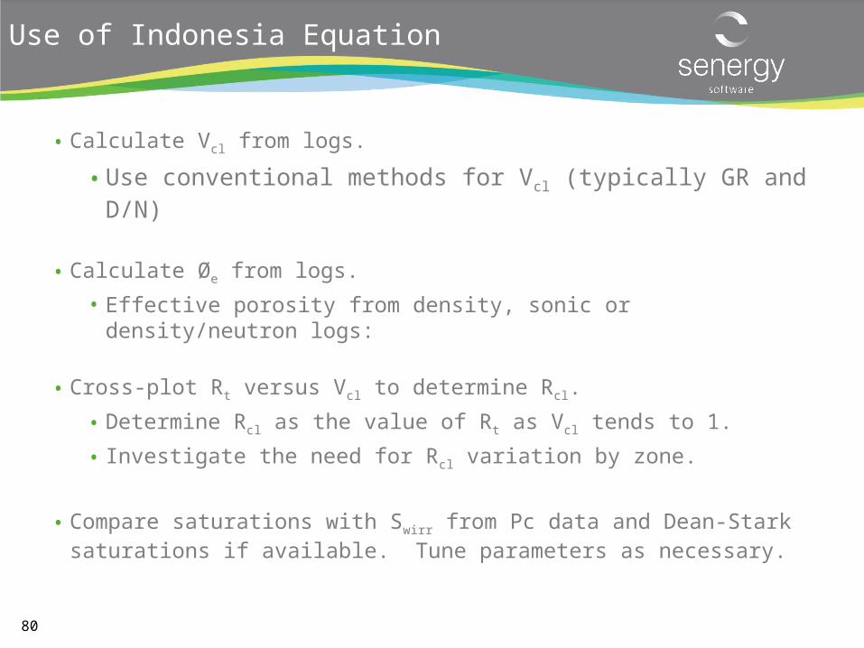
Use of Indonesia Equation

• Calculate Vcl from logs.

• Use conventional methods for Vcl (typically GR and D/N)

• Calculate Øe from logs.

• Effective porosity from density, sonic or density/neutron logs:

• Cross-plot Rt versus Vcl to determine Rcl.

• Determine Rcl as the value of Rt as Vcl tends to 1.

• Investigate the need for Rcl variation by zone.

• Compare saturations with Swirr from Pc data and Dean-Stark saturations if available. Tune parameters as necessary.

81

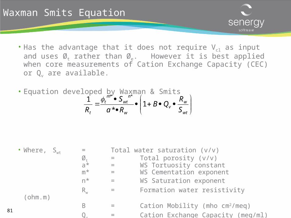
Waxman Smits Equation

• Has the advantage that it does not require Vcl as input and uses Øt rather than Øe. However it is best applied when core measurements of Cation Exchange Capacity (CEC) or Qv are available.

• Equation developed by Waxman & Smits

• Where, Swt = Total water saturation (v/v)Øt = Total porosity (v/v)a* = WS Tortuosity constantm* = WS Cementation exponentn* = WS Saturation exponent

Rw = Formation water resistivity (ohm.m)B = Cation Mobility (mho cm2/meq)

Qv = Cation Exchange Capacity (meq/ml)

wt

wv

w

nwt

mt

t S

RQB

Ra

S

R1

*

1**

82

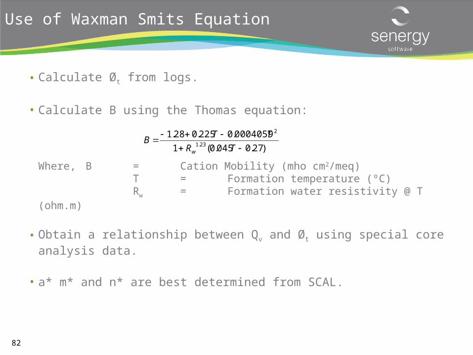
Use of Waxman Smits Equation

• Calculate Øt from logs.

• Calculate B using the Thomas equation:

Where, B = Cation Mobility (mho cm2/meq)T = Formation temperature (ºC)Rw = Formation water resistivity @ T (ohm.m)

• Obtain a relationship between Qv and Øt using special core analysis data.

• a* m* and n* are best determined from SCAL.

)27.0045.0(1

0004059.0225.028.123.1

2

TR

TTB

w

83

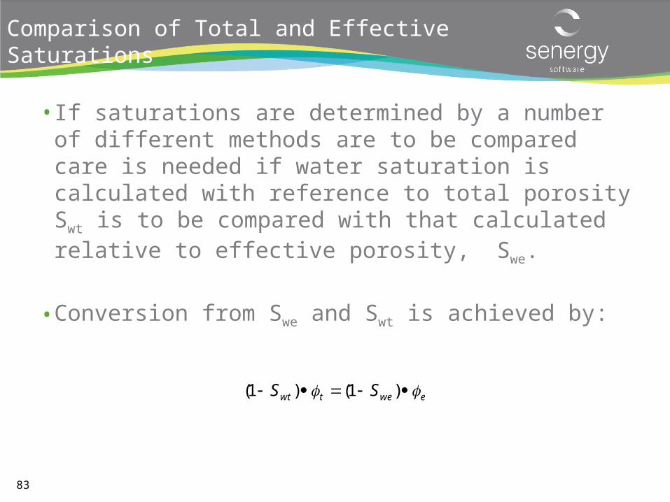
Comparison of Total and Effective Saturations

• If saturations are determined by a number of different methods are to be compared care is needed if water saturation is calculated with reference to total porosity Swt is to be compared with that calculated relative to effective porosity, Swe.

• Conversion from Swe and Swt is achieved by:

ewetwt SS )1()1(

84

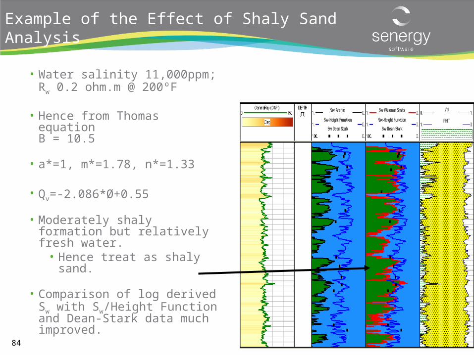
Example of the Effect of Shaly Sand Analysis

• Water salinity 11,000ppm; Rw 0.2 ohm.m @ 200ºF

• Hence from Thomas equation B = 10.5

• a*=1, m*=1.78, n*=1.33

• Qv=-2.086*Ø+0.55

• Moderately shaly formation but relatively fresh water.

• Hence treat as shaly sand.

• Comparison of log derived Sw with Sw/Height Function and Dean-Stark data much improved.

www.senergyworld.com

Water Saturation Calculation in IP

86

Water Saturation Models

• Selecting the default Sw equation on the Phi/Sw setup window changes the default plot.

• The interactive default plot has special interactive parameter lines and crossplot depending on the setup.

• Changing the default Sw equation will not change the Sw equation for any already created zones.

87

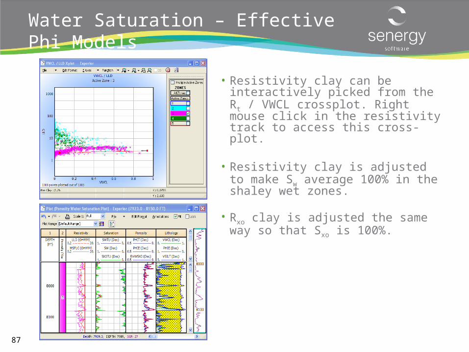
Water Saturation – Effective Phi Models

• Resistivity clay can be interactively picked from the Rt / VWCL crossplot. Right mouse click in the resistivity track to access this cross-plot.

• Resistivity clay is adjusted to make Sw average 100% in the shaley wet zones.

• Rxo clay is adjusted the same way so that Sxo is 100%.

88

Water Saturation – Total Phi Models

• Total porosity• øt = øe + Vcl x øtclay

• Clay porosity Øtclay

• Entered as a fixed parameter

• Calculated from density dry and wet clay parameters

• Best method of obtaining this is from core analysis data

89

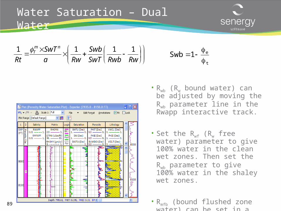
Water Saturation – Dual Water

• Rwb (Rw bound water) can be adjusted by moving the Rwb parameter line in the Rwapp interactive track.

• Set the Rwf (Rw free water) parameter to give 100% water in the clean wet zones. Then set the Rwb parameter to give 100% water in the shaley wet zones.

• Rmfb (bound flushed zone water) can be set in a similar fashion.

RwRwbSwT

Swb

Rwa

SwT

Rt

nmT 1111

t

e1Swb

90

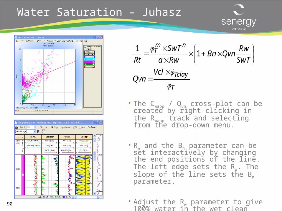
Water Saturation – Juhasz

• The Cwapp / Qvn cross-plot can be created by right clicking in the Rwapp track and selecting from the drop-down menu.

• Rw and the Bn parameter can be set interactively by changing the end positions of the line. The left edge sets the Rw. The slope of the line sets the Bn parameter.

• Adjust the Rw parameter to give 100% water in the wet clean zones. Adjust the Bn parameter on the crossplot to give 100% water in the shaley wet zones.

T

Tclay

nmT

VclQvn

SwT

RwQvnBn

Rwa

SwT

Rt

11

91

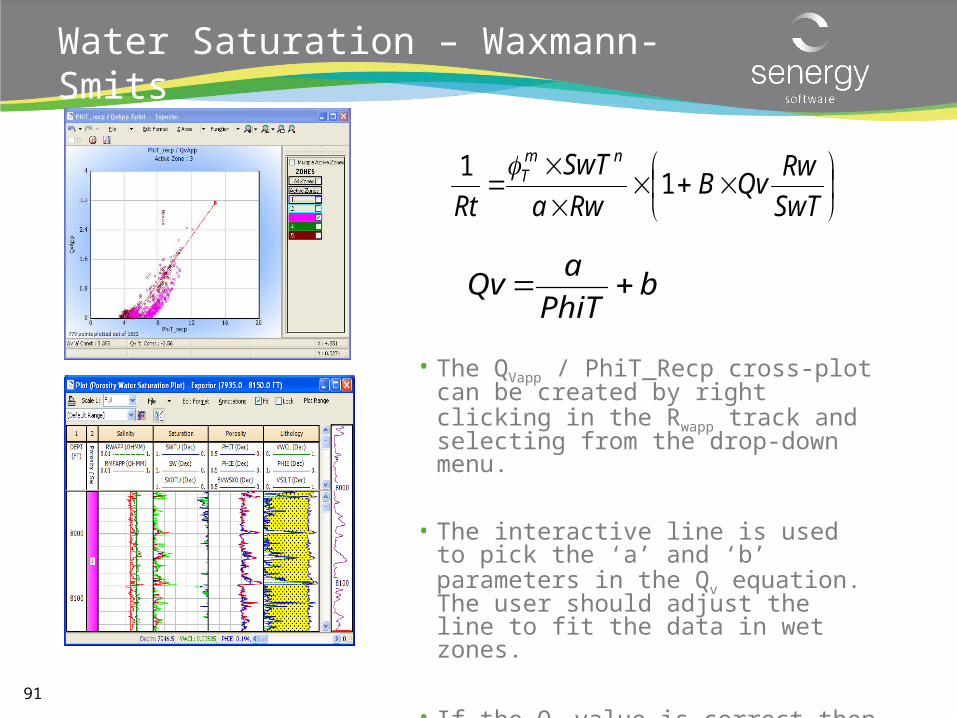
Water Saturation – Waxmann-Smits

• The QVapp / PhiT_Recp cross-plot can be created by right clicking in the Rwapp track and selecting from the drop-down menu.

• The interactive line is used to pick the ‘a’ and ‘b’ parameters in the Qv equation. The user should adjust the line to fit the data in wet zones.

• If the Qv value is correct then SwT should read 100% in the shaley wet zones.

SwT

RwQvB

Rwa

SwT

Rt

nmT 1

1

bPhiT

aQv

92

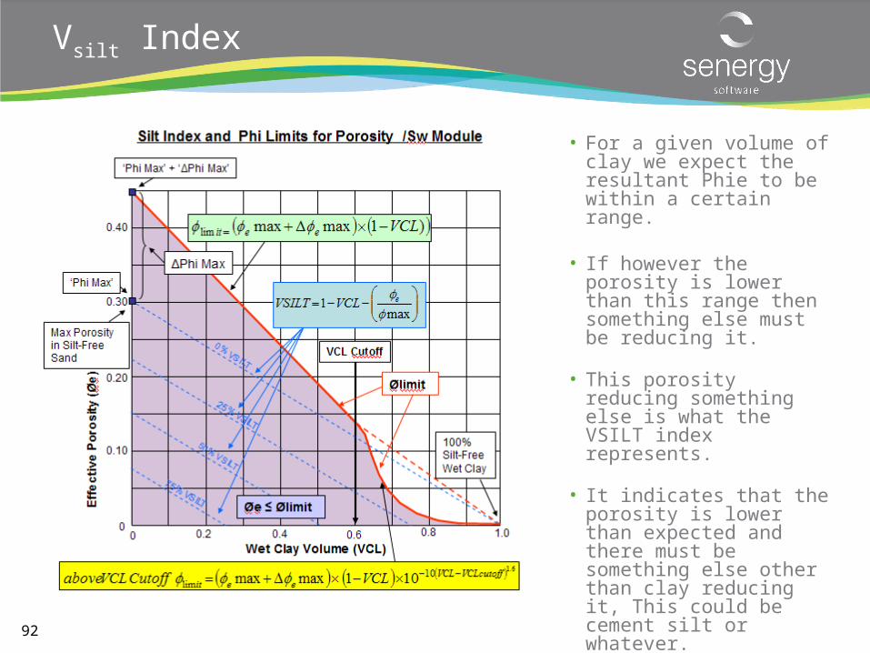
Vsilt Index

• For a given volume of clay we expect the resultant Phie to be within a certain range.

• If however the porosity is lower than this range then something else must be reducing it.

• This porosity reducing something else is what the VSILT index represents.

• It indicates that the porosity is lower than expected and there must be something else other than clay reducing it, This could be cement silt or whatever.

• It is purely for display purposes and does not impact on porosity or Sw calculations.

93

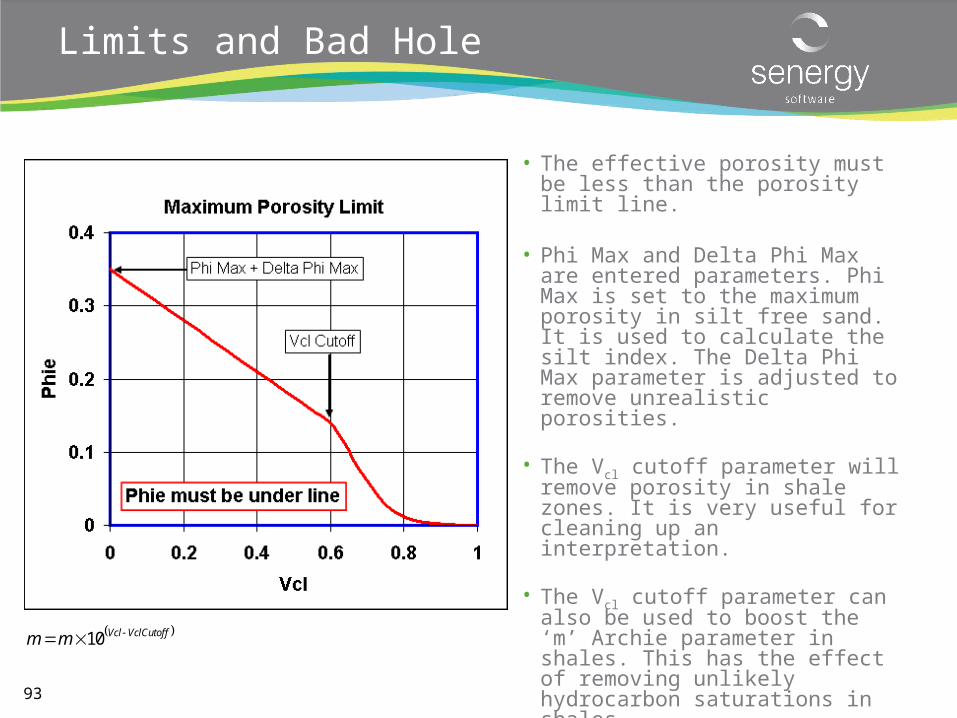
Limits and Bad Hole

• The effective porosity must be less than the porosity limit line.

• Phi Max and Delta Phi Max are entered parameters. Phi Max is set to the maximum porosity in silt free sand. It is used to calculate the silt index. The Delta Phi Max parameter is adjusted to remove unrealistic porosities.

• The Vcl cutoff parameter will remove porosity in shale zones. It is very useful for cleaning up an interpretation.

• The Vcl cutoff parameter can also be used to boost the ‘m’ Archie parameter in shales. This has the effect of removing unlikely hydrocarbon saturations in shales.

m m Vcl VclCutoff 10

94

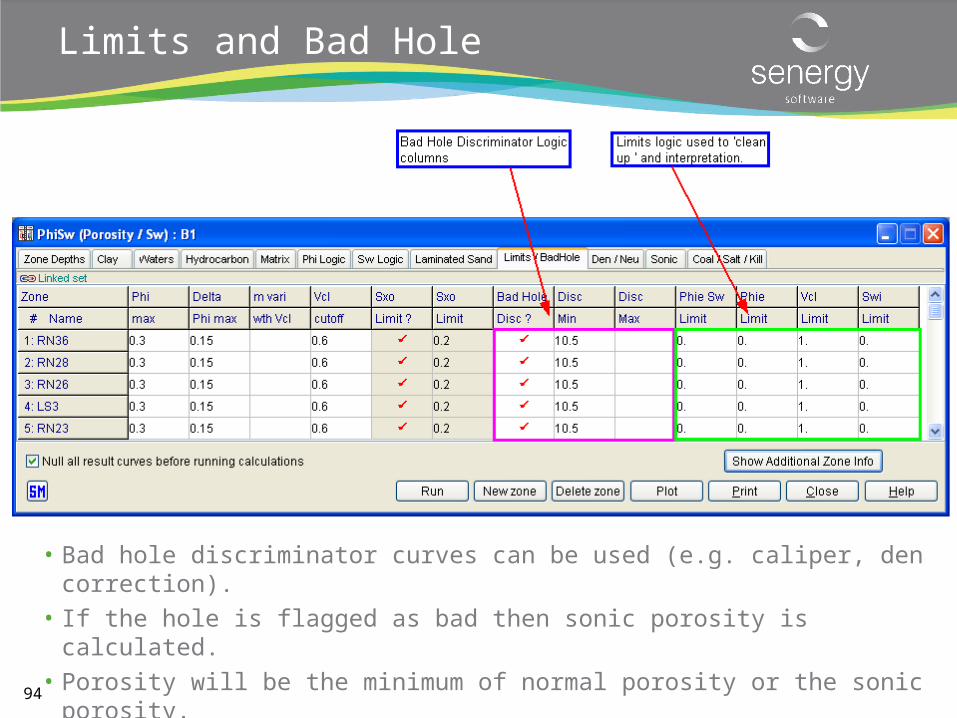
Limits and Bad Hole

• Bad hole discriminator curves can be used (e.g. caliper, den correction).

• If the hole is flagged as bad then sonic porosity is calculated.

• Porosity will be the minimum of normal porosity or the sonic porosity.

• Normal porosity limits are still applied.

95

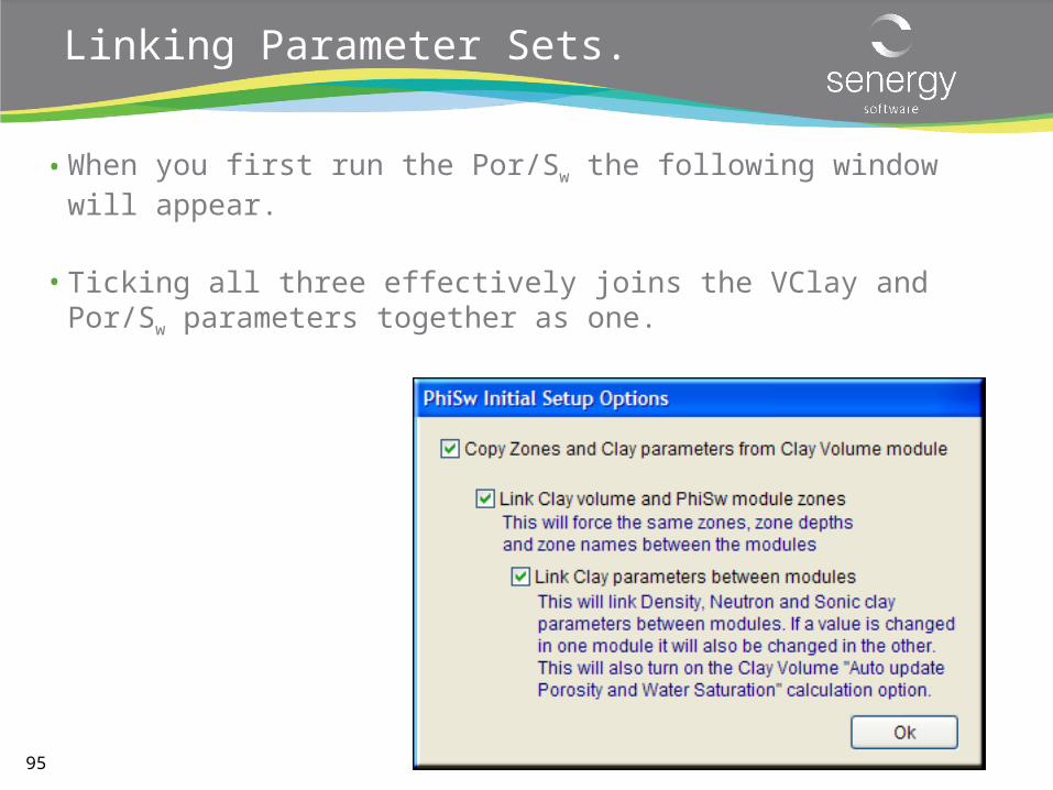
Linking Parameter Sets.

• When you first run the Por/Sw the following window will appear.

• Ticking all three effectively joins the VClay and Por/Sw parameters together as one.

96

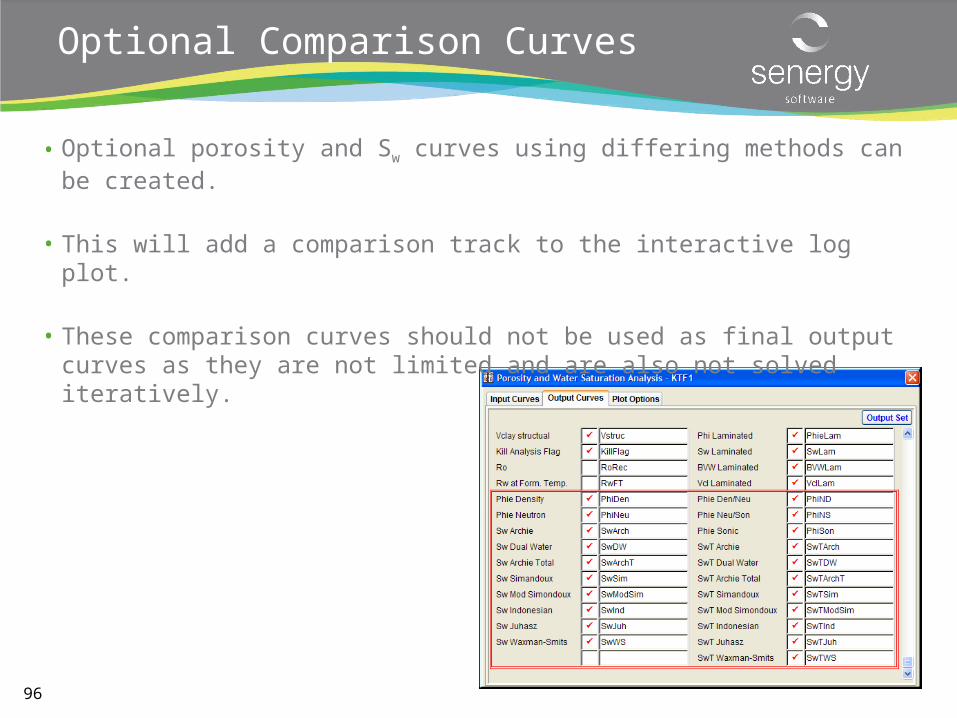
Optional Comparison Curves

• Optional porosity and Sw curves using differing methods can be created.

• This will add a comparison track to the interactive log plot.

• These comparison curves should not be used as final output curves as they are not limited and are also not solved iteratively.

www.senergyworld.com

Deterministic Petrophysics: Net and Pay

98

Basic Interpretation Workflow Net and Pay Definition

• Gross Rock: • Comprises all rock in the evaluation interval.

• Net Sand:• Comprises those rocks which may have useful reservoir

properties.• Sand is a generic oilfield term for lithologically clean sedimentary

rock.• Determined using a Vclay cut-off.

• Net Reservoir• Comprises those rocks which do have useful reservoir properties.• Determined using a porosity cut-off on Net sand.

• Net Pay:• Comprises the net sands that contain hydrocarbon.• Determined using a water saturation cut-off on Net Reservoir

99

Net Reservoir Determination

• Western Petroleum Industry Practice• Traditionally adopts rule of thumb cut-offs for the evaluation of net

pay.• The arbitrary nature of the cut-offs is recognised.• Usually the cut-offs have been selected to correspond to fixed

permeability values:• 0.1 mD for gas reservoirs• 1.0 mD for oil reservoirs

• These nominal cut-offs are still commonly used.

• Because permeability is not measured by logs the normal practice is to relate core permeability to porosity and/or other log-derivable parameters.

• The precise type of permeability used to specify the cut-off is not defined.

100

Determining Net Sand cut-offs

• Determine using a Vcl cut off.

• The cut off is generally arbitrary and of the form Vcl<= Cut-off.

• The sensitivity of Net Sand count to the cut-off is generally examined by determining the net-sand for a range of cut-offs. The cut off should be determined in an insensitive region of the sensitivity plot if possible.

• Cut-offs should be validated by comparison of resulting Net sand with that observed in core.

• If sands with laminations below log resolution are encountered it is possible no net reservoir will be resolved. In these cases cut-offs may not be appropriate

101

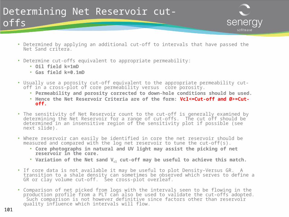
Determining Net Reservoir cut-offs

• Determined by applying an additional cut-off to intervals that have passed the Net Sand critera.

• Determine cut-offs equivalent to appropriate permeability:• Oil field k=1mD • Gas field k=0.1mD

• Usually use a porosity cut-off equivalent to the appropriate permeability cut-off in a cross-plot of core permeability versus core porosity.

• Permeability and porosity corrected to down-hole conditions should be used.• Hence the Net Reservoir Criteria are of the form: Vcl<=Cut-off and Ø>=Cut-off.

• The sensitivity of Net Reservoir count to the cut-off is generally examined by determining the Net Reservoir for a range of cut-offs. The cut off should be determined in an insensitive region of the sensitivity plot if possible (see next slide).

• Where reservoir can easily be identified in core the net reservoir should be measured and compared with the log net reservoir to tune the cut-off(s).

• Core photographs in natural and UV light may assist the picking of net reservoir in the core.• Variation of the Net sand Vcl cut-off may be useful to achieve this match.

• If core data is not available it may be useful to plot Density–Versus GR. A transition to a shale density can sometimes be observed which serves to define a GR or clay volume cut-off. See cross-plot overleaf.

• Comparison of net picked from logs with the intervals seen to be flowing in the production profile from a PLT can also be used to validate the cut-offs adopted. Such comparison is not however definitive since factors other than reservoir quality influence which intervals will flow.

102

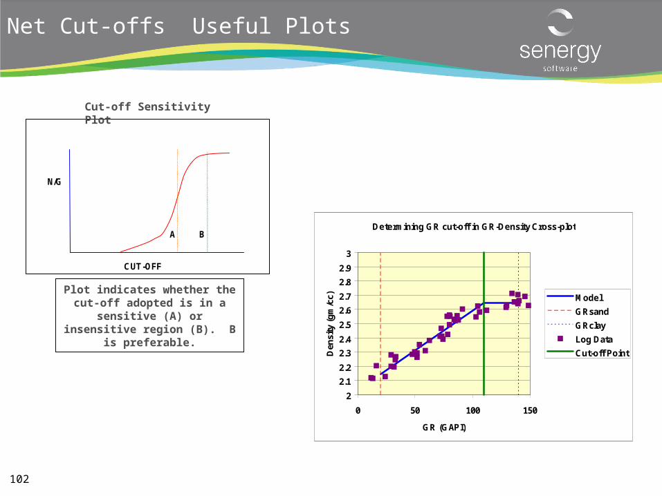
Net Cut-offs Useful Plots

Determining GR cut-off in GR-Density Cross-plot

2

2.1

2.2

2.3

2.4

2.5

2.6

2.7

2.8

2.9

3

0 50 100 150

GR (GAPI)

Den

sity

(g

m/c

c) Model

GRsand

GRclay

Log Data

Cut-off Point

N/G

A B

CUT-OFF

Plot indicates whether the cut-off adopted is in a sensitive (A) or

insensitive region (B). B is preferable.

Cut-off Sensitivity Plot

103

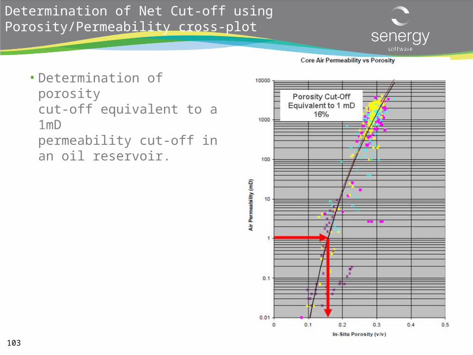
Determination of Net Cut-off using Porosity/Permeability cross-plot

• Determination of porositycut-off equivalent to a 1mDpermeability cut-off in an oil reservoir.

103

104

• Net Pay is determined by the addition of a water saturation cut off to the Net Reservoir Criteria: Vcl<=Cut-off and Ø>=Cut-off.

• Net Pay defines the potentially productive portion of the reservoir.

• The cut off Sw is in most cases largely arbitrary (typically 50% - 60%).

• Relative permeability curves can be used to inform the choice of Sw cut-off ~ Sw Critical.

• Net Reservoir and Net Pay are used to determine Reservoir summary zonal averages.

• Versions of the log interpreted curves, set to null outside the net sands, are often generated.

• Numerical Flags are usually created for Net Sand, Net Reservoir and Net Pay.

Determination of Net Pay

www.senergyworld.com

Reservoir Summaries in IP

106

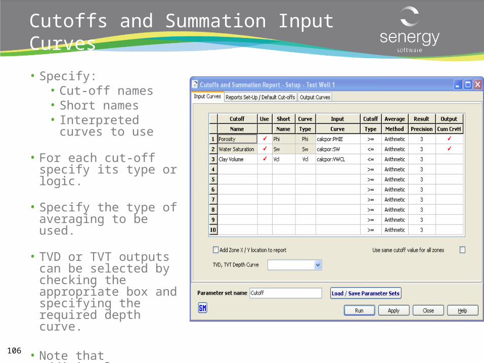
Cutoffs and Summation Input Curves

• Specify:• Cut-off names• Short names• Interpreted curves to

use

• For each cut-off specify its type or logic.

• Specify the type of averaging to be used.

• TVD or TVT outputs can be selected by checking the appropriate box and specifying the required depth curve.

• Note that additional curves can be selected for averaging without being used as cut-offs.

107

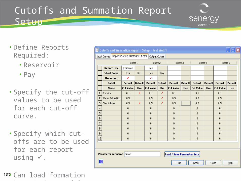
Cutoffs and Summation Report Setup

• Define Reports Required:• Reservoir• Pay

• Specify the cut-off values to be used for each cut-off curve.

• Specify which cut-offs are to be used for each report using .

• Can load formation tops to be used in averaging via Load/Save ParameterSets

108

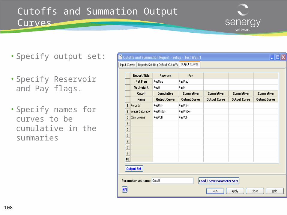
Cutoffs and Summation Output Curves

• Specify output set:

• Specify Reservoir and Pay flags.

• Specify names for curves to be cumulative in the summaries

109

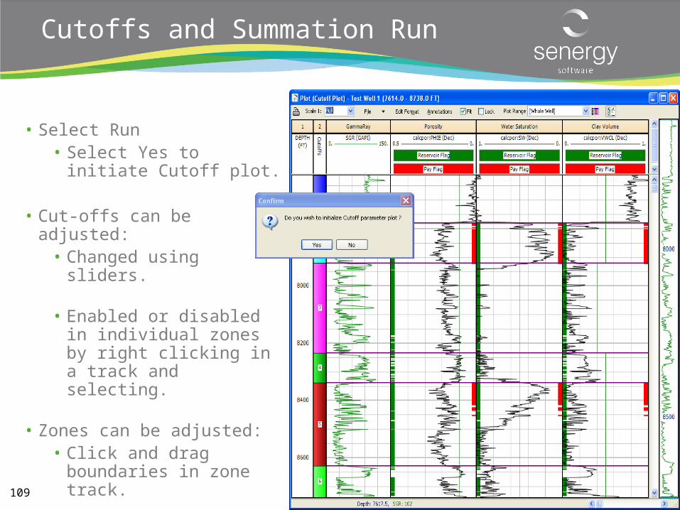
Cutoffs and Summation Run

• Select Run• Select Yes to initiate Cutoff

plot.

• Cut-offs can be adjusted:• Changed using sliders.

• Enabled or disabled in individual zones by right clicking in a track and selecting.

• Zones can be adjusted:• Click and drag boundaries in

zone track.

• Zones can be deleted if required.

110

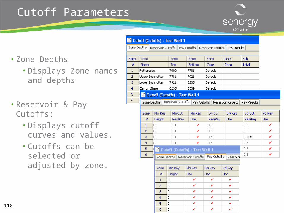
Cutoff Parameters

• Zone Depths• Displays Zone names and

depths

• Reservoir & Pay Cutoffs:• Displays cutoff curves and

values.• Cutoffs can be selected or

adjusted by zone.

111

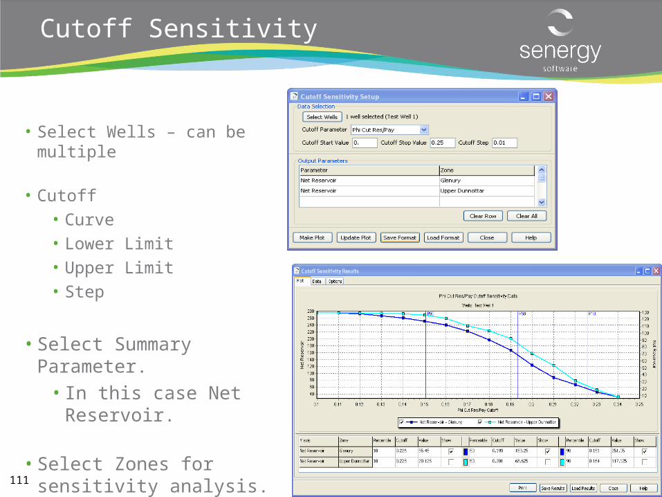
Cutoff Sensitivity

• Select Wells – can be multiple

• Cutoff

• Curve

• Lower Limit

• Upper Limit

• Step

• Select Summary Parameter.• In this case Net Reservoir.

• Select Zones for sensitivity analysis.

• Make Plot.

www.senergyworld.com

Parameter Sets

113

Parameter Sets

• Parameter Sets are created when any of the zonable interpretation modules are run.

• Clay Volume• Porosity and Water Saturation• Cutoffs and Summation• Mineral Solver• Basic Log Analysis• NMR Interpretation• TDT Standalone• TDT Time Lapse• Pore Pressure Gradient• User Programs

114

Parameter Sets

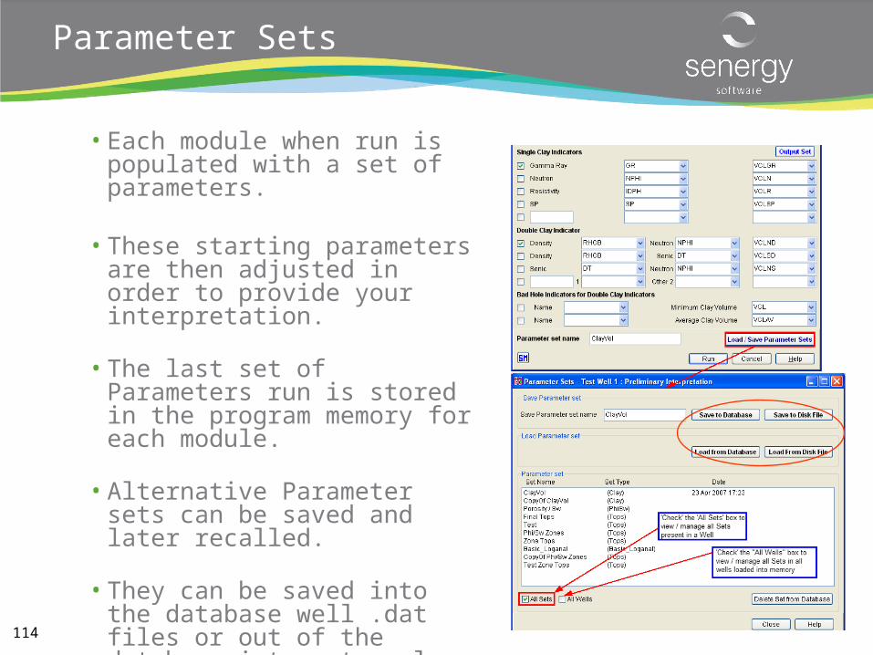
• Each module when run is populated with a set of parameters.

• These starting parameters are then adjusted in order to provide your interpretation.

• The last set of Parameters run is stored in the program memory for each module.

• Alternative Parameter sets can be saved and later recalled.

• They can be saved into the database well .dat files or out of the database into external ASCII disk files.

115

Parameter Sets

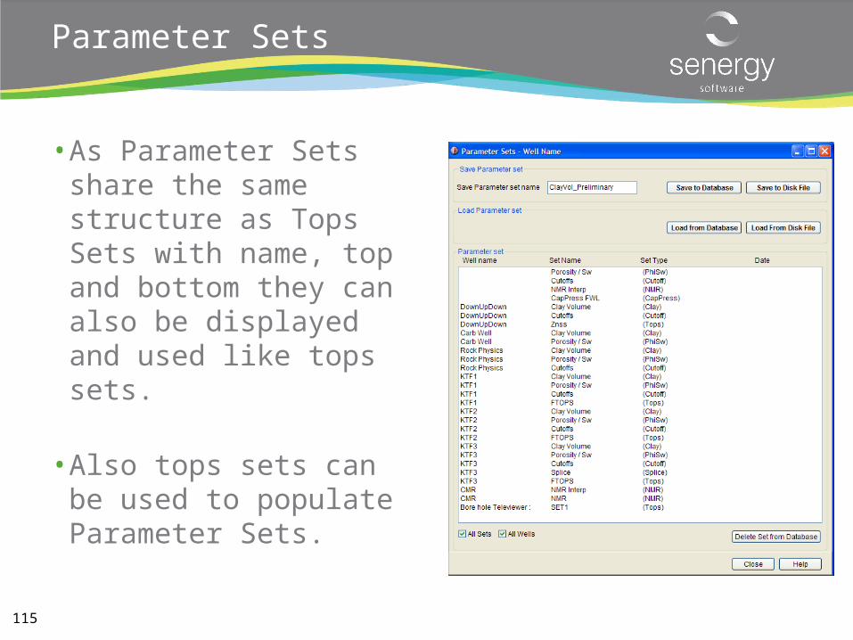
• As Parameter Sets share the same structure as Tops Sets with name, top and bottom they can also be displayed and used like tops sets.

• Also tops sets can be used to populate Parameter Sets.

116

Delete Parameter Sets [Well]

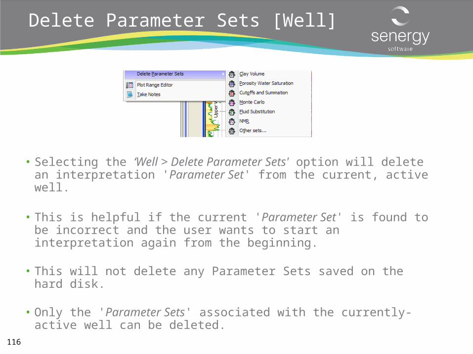
• Selecting the ‘Well > Delete Parameter Sets' option will delete an interpretation 'Parameter Set' from the current, active well.

• This is helpful if the current 'Parameter Set' is found to be incorrect and the user wants to start an interpretation again from the beginning.

• This will not delete any Parameter Sets saved on the hard disk.

• Only the 'Parameter Sets' associated with the currently-active well can be deleted.

117

Multi-well Parameter Distribution [Multi-Well]

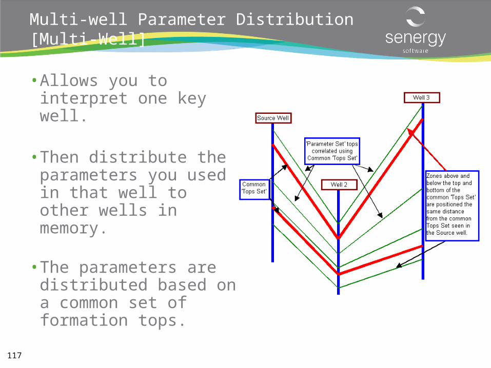
• Allows you to interpret one key well.

• Then distribute the parameters you used in that well to other wells in memory.

• The parameters are distributed based on a common set of formation tops.

118

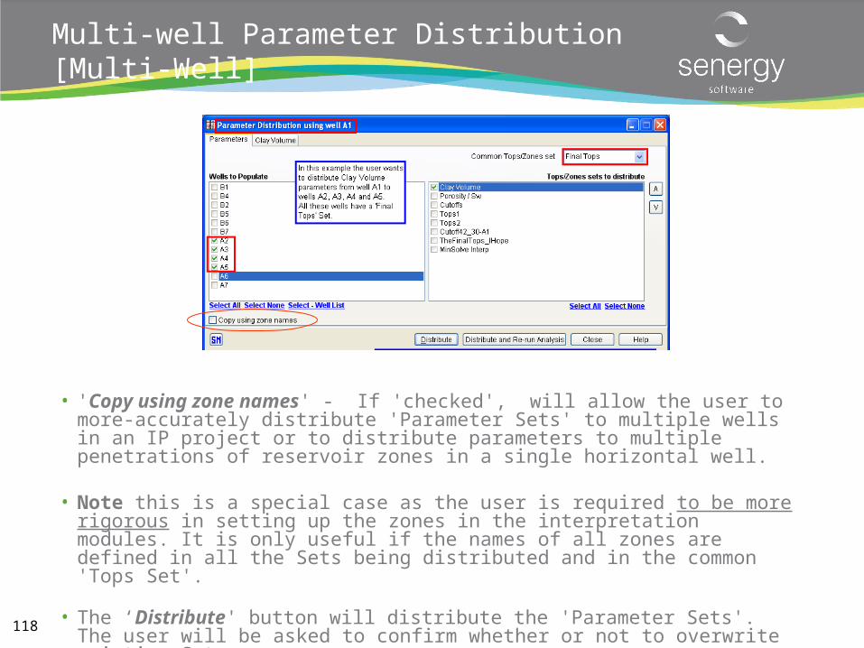
Multi-well Parameter Distribution [Multi-Well]

• 'Copy using zone names' -  If 'checked',  will allow the user to more-accurately distribute 'Parameter Sets' to multiple wells in an IP project or to distribute parameters to multiple penetrations of reservoir zones in a single horizontal well.

• Note this is a special case as the user is required to be more rigorous in setting up the zones in the interpretation modules. It is only useful if the names of all zones are defined in all the Sets being distributed and in the common 'Tops Set'.

• The ‘Distribute' button will distribute the 'Parameter Sets'. The user will be asked to confirm whether or not to overwrite existing Sets.

119

Multi-well 3-D Parameter viewer

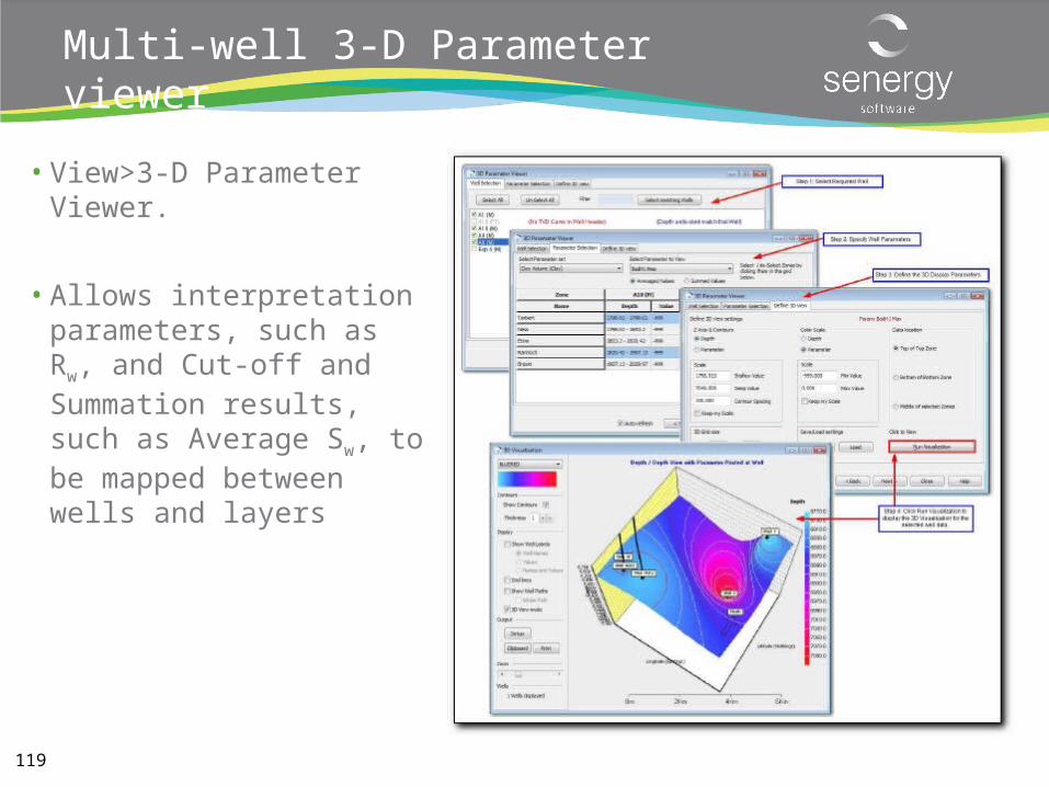
• View>3-D Parameter Viewer.

• Allows interpretation parameters, such as Rw, and Cut-off and Summation results, such as Average Sw, to be mapped between wells and layers

120

Curve History

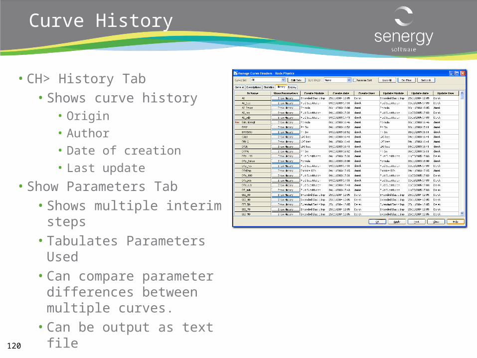
• CH> History Tab• Shows curve history

• Origin

• Author

• Date of creation

• Last update

• Show Parameters Tab• Shows multiple interim steps• Tabulates Parameters Used• Can compare parameter

differences between multiple curves.

• Can be output as text file

121

Movie

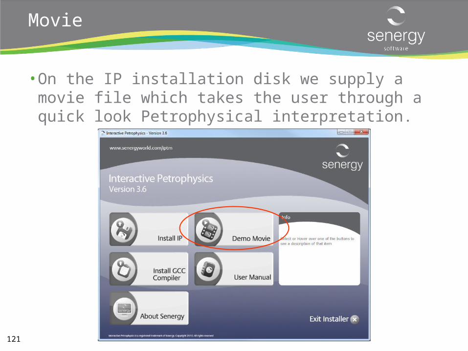
• On the IP installation disk we supply a movie file which takes the user through a quick look Petrophysical interpretation.

122

Summary

• Over the past few days you should have learnt:• How IP’s Database is structured• Loading data in from external files (LAS etc)• Presenting Data (Logplots, Crossplots, Histograms)• Editing Data (Depth shifting, splicing etc)• How to Run calculations (single or multi-line formulas etc)• Use the clay volume, Por/Sw and Cutoff deterministic petrophysics

modules to derive Vclay, Porosity, Sw and N/G • Understand parameter sets (how to save and recall them)• Use Multi-Well workflows

• We hope you have enjoyed this insight into the basic functionality of IP.

Thank You

123

Interactive Petrophysics (IP4)Advanced

124

Interactive Petrophysics Advanced: Contents

• Statistical Curve and Facies Analysis: Fuzzy Logic in IP

• Statistical Curve Prediction: Multi-linear Regression in IP

• Statistical Curve Prediction: Neural Nets in IP

• Facies Prediction: Cluster Analysis in IP

• Monte Carlo Analysis in IP

• Capillary Pressure and Saturation-Height• Principals• Execution in IP

• Pore Pressure Calculations in IP

125

Fuzzy Logic

Statistical Curve & Facies Prediction

126

Fuzzy Logic

• Fuzzy logic is the logic of partial truths• The statement, today is sunny

• 100% true if there are no clouds • 80% true if there are a few clouds • 50% true if it's hazy • 0% true if it rains all day

• This is mathematics of probabilities• If we can work out the probability of each event outcome then

we can predict the most likely result

• More details read ‘The Application of the Mathematics of Fuzzy Logic to Petrophysics’ - Steve Cuddy

127

Fuzzy Logic

• Used for predicting petrophysical properties from any combination of data.

• Predict: Facies, Permeability, Density, Sonic etc.• Use: Raw logs, Petrophysical results, Core results

• Two basic modes of prediction depending on input data.• Fixed value input data: Facies• Continuous value data: Log curves, Core permeability

128

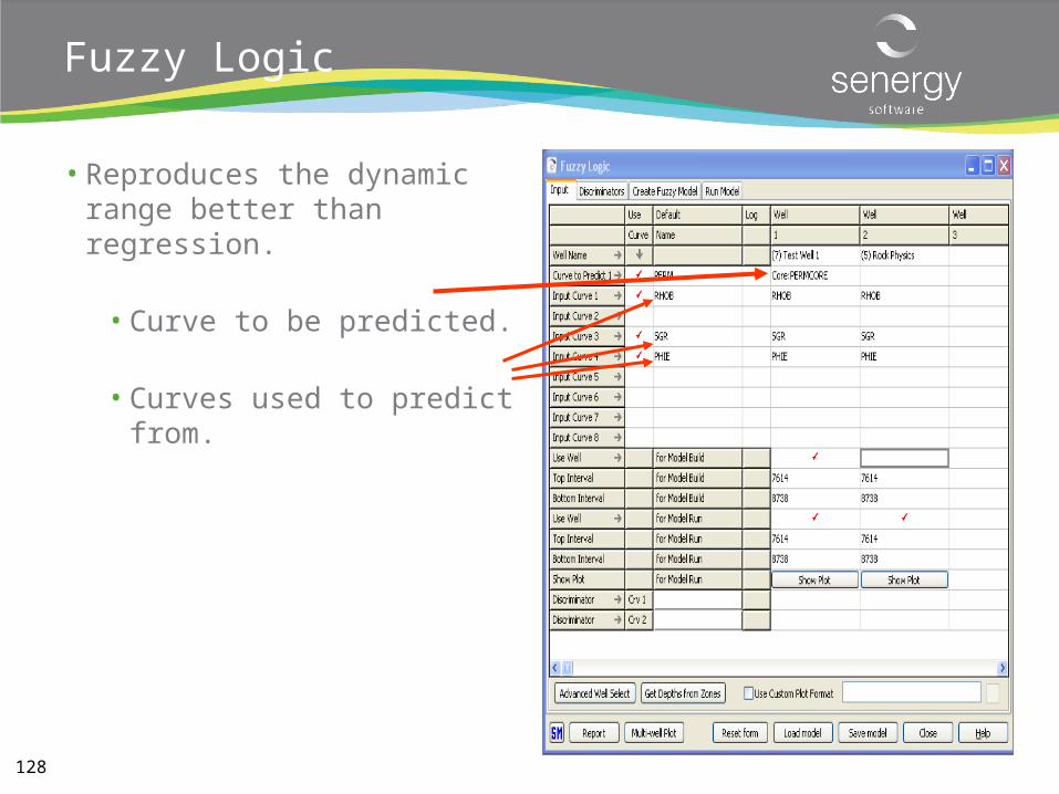
Fuzzy Logic

• Reproduces the dynamic range better than regression.

• Curve to be predicted.

• Curves used to predict from.

128