DETERMINANTS OF REDISTRIBUTIVEPOLITICS:

An Empirical Analysis of Land Reforms in WestBengal, India1

Pranab Bardhan2 and Dilip Mookherjee3

Revised version: June 28, 2009

Abstract

We investigate political determinants of land reform implementation in the

Indian state of West Bengal. Using a village panel spanning 1974–98, we do not

find evidence supporting the hypothesis that land reforms were positively and

monotonically related to control of local governments by a Left-front coalition

vis-a-vis the right-centrist Congress party, combined with lack of commitment

to policy platforms. Instead, the evidence is consistent with a quasi-Downsian

1We thank the MacArthur Foundation Inequality Network for funding the data collection. We are

grateful to various officials of the West Bengal government for giving us access to the data; to Sankar

Bhaumik and Sukanta Bhattacharya of the Department of Economics, Calcutta University who led

the village survey teams, and Indrajit Mallick for helping us collect the election data. For useful

comments and suggestions we thank Debu Bandyopadhyay, Abhijit Banerjee, Partha Chatterjee,

Asim Dasgupta, Esther Duflo, Andy Foster, Penny Goldberg, Saumitra Jha, Michael Kremer, Kevin

Lang, Nolan McCarty, Kaivan Munshi and two anonymous referees. Alfredo Cuecuecha, Nobuo

Yoshida, Amaresh Tiwari, Satadru Bhattacharya helped with the preliminary data work. Mon-

ica Parra Torrado and Ramiro de Elejalde subsequently provided invaluable research assistance.

Mookherjee thanks the John Henry Simon Guggenheim Foundation for funding a sabbatical year

when part of this research was conducted. The paper has benefited from the comments of seminar

participants at Jadavpur, MIT, PennState, Princeton, Stanford, Toulouse, World Bank, MacArthur

Inequality network, and the Center for Studies in Social Science, Calcutta.2Department of Economics, University of California, Berkeley; bardhan@econ.berkeley.edu3Department of Economics, Boston University; dilipm@bu.edu

1

theory stressing the role of opportunism (re-election concerns) and electoral

competition.

2

DETERMINANTS OF REDISTRIBUTIVEPOLITICS:

An Empirical Analysis of Land Reforms in WestBengal, India

June 28 2009

Abstract

We investigate political determinants of land reform implementation in the

Indian state of West Bengal. Using a village panel spanning 1974–98, we do not

find evidence supporting the hypothesis that land reforms were positively and

monotonically related to control of local governments by a Left-front coalition

vis-a-vis the right-centrist Congress party, combined with lack of commitment

to policy platforms. Instead, the evidence is consistent with a quasi-Downsian

theory stressing the role of opportunism (re-election concerns) and electoral

competition.

Keywords: land reform, electoral competition, political ideology, Downsian the-

ory, West Bengal

1

1 Introduction

In this paper we investigate political determinants of land reform implementation in

the Indian state of West Bengal since the late 1970s. There is now considerable evi-

dence that land reforms have significant potential for simultaneously reducing poverty

and promoting agricultural growth in many developing countries, including India.1

Despite this, the extent of land reforms enacted typically remains small in most de-

veloping countries relative to what could potentially be achieved. The causes are

rooted mainly in lack of political will, the power of landed interests, and formidable

legal and administrative barriers (see, for example, the review of the land reform ex-

perience of different Indian states by Appu (1996)).2 It can be argued, however, that

persistence of legal and administrative barriers owe ultimately to lack of political will:

when governments really do intend to carry out land reforms they can improve the

land records, push through legislative reforms to close loopholes, and pursue neces-

sary litigation. From this standpoint political will is the fundamental sine qua non.

Accordingly there is an urgent need to understand better the determinants of political

will of elected governments to implement land reforms.

Theoretical models of political economy are frequently classified (see, e.g., Roe-

mer (2001)) according to the motivation of competing parties or candidates, as either

1For instance, there is evidence that small farms are more productive than large farms (e.g.,

Bardhan (1973), Berry and Cline (1979), Binswanger and Rosenzweig (1986, 1993), Binswanger,

Deininger and Feder (1993)), that owner-cultivated farms are more productive than tenant farms

(Bell (1977), Sen (1981), Shaban (1987)), both of which imply agricultural output would rise fol-

lowing redistribution of land. Moreover, Banerjee, Gertler and Ghatak (2002) argue that protection

of sharecroppers against eviction and regulating sharecropping contracts in West Bengal during the

period we study caused significant growth in agricultural yields. Besley and Burgess (2000) find

that implementation of land reforms (particularly with respect to tenancy protection legislation) in

Indian states between 1958 and 1992 led to significant reductions in rates of rural poverty.2The latter stem from poor state of land records, pervasiveness of legal loopholes and legal systems

ill-equipped to deal with large volumes of litigation.

2

purely opportunistic (where they care only about the probability of winning elec-

tions), or where they have intrinsic policy preferences derived from their ideology

(defined broadly to include interests of constituents they represent). Accordingly,

these respective approaches differ in their emphasis on the importance of electoral

competition relative to the political ideology of elected officials in explaining policy

choices observed in democracies. Models in the tradition of Downs (1957) which are

based on the former assumption stress the role of competition and electoral oppor-

tunism.3 The Downsian view emphasizes the role of competitive electoral incentives:

that political will is driven ultimately by policy preferences of voters and special

interest groups, not elected officials.

In contrast, ideology-based theories of politics which trace their origin to Lipset

(1960) and Wittman (1973) have recently received prominence in citizen-candidate

models of Osborne and Slivinski (1996) and Besley and Coate (1997). These are

based on the assumption that candidates cannot commit to their policy platforms in

advance of elections, and are myopic in that they ignore implications of current policy

choices for future re-election prospects. These theories predict that policy choices of

elected candidates are entirely determined by their ‘ideology’ or policy preferences.

Accordingly predicting policy choices translates into predicting electoral success of

parties or candidates with heterogenous policy preferences, rather than the intensity

of political competition or preferences of median voters.

3These include models of electoral competition extended to include probabilistic voting

(Lindbeck-Weibull (1987)) and special interest groups (Baron (1994), Grossman-Helpman (1996)).

Standard formulations of this model assume that candidates have no intrinsic policy preferences,

and that they commit to policy platforms in advance of elections. In a two candidate setting the

outcome is policy convergence: both candidates select the same policy owing to their common vote-

maximization objective. In the presence of interest groups such convergence does not obtain. But

as indicated later in the paper, the predictions of such an extension with interest groups is similar to

the quasi-Downsian model developed in this paper: increased competition makes both parties more

responsive to voter preferences.

3

Not much is known, however, about the relative importance of electoral compe-

tition and heterogenous policy preferences of elected officials, in determining redis-

tributive effort of governments. This is important in terms of understanding the way

that democracies promote responsiveness of government to voter needs and prefer-

ences. The nature of land reform and political competition in West Bengal over the

past quarter century provides an opportunity to test the two competing theories in

a simple and compelling way. There have been two principal competing parties in

West Bengal with distinct political ideologies and constituencies: a coalition of Leftist

parties led by the Communist Party of India (Marxist) (CPIM) with a strong polit-

ical commitment to land reform, and a centrist Indian National Congress (INC) (or

offshoots such as the Trinamul Congress) that has traditionally represented interests

of big landowners in rural areas. Given the nature of these traditional ideologies and

key constituencies of the two parties, the ideology hypothesis predicts that the extent

of land reform should rise as the composition of local governments (key implementing

agencies in West Bengal villages) swings in favor of the Left Front coalition. In con-

trast, the Downsian theory predicts these should have no effect. If the latter approach

is extended to incorporate policy-nonconvergence across competing parties owing to

moral hazard (or special interest influence), we show in Section 3 of the paper that

the resulting quasi-Downsian approach predicts an inverted-U relationship between

Left control of local governments and land reform implementation. In other words,

variations in land reform implementation are explained, if at all, by the extent of

electoral competition.

Simple regressions or plots between land reform implementation and the Left

share of local governments (shown in Section 2) fail to show any significant positive

relationship, in either cross-village data or a village panel. Instead, the raw pattern

in the data resembles an inverted-U, suggesting the role of political competition.

Section 3 presents a theoretical model which nests the principal hypotheses as

special cases. The model is characterized by probabilistic voting, co-existence of

4

heterogenous redistributive preferences of two competing parties, and a mixture of

opportunism (i.e., re-election concerns) and (current) rent-seeking motives of their

candidates. In particular, elected officials may be subject to rent-seeking or other

forms of political moral hazard (e.g., land reforms require costly administrative effort

on the part of the officials).4 Under specific parameter values (reflecting low hetero-

geneity of redistributive preferences, relative to opportunistic motives), interactions

between moral hazard and electoral competition generate an inverted-U relationship:

a more lop-sided electoral contest (arising from more skewed preferences amongst

voters in favor of one party) translates into lower redistributive effort by the dom-

inant party. With greater heterogeneity of policy preferences, there is a monotone

relationship between redistributive effort and party composition, as predicted by a

pure citizen-candidate model.

The theoretical model is thereafter used to guide the empirical specification. The

impact of rising Left share of local government seats on land reform reflects rising

competitive strength of the Left Front coalition vis-a-vis the Congress, as represented

by the realization of voter loyalty shocks. The latter can be proxied by differences

in vote shares between the two parties in preceding elections to the state Assembly

(rather than the local government elections), averaging across different constituencies

in a district. In other words, the relative popularity of the two parties in the region in

which the village happens to be located, is reflected in this difference in vote shares

in Assembly elections (typically held two years prior to local government elections).

The competition effect generated by the hybrid quasi-Downsian model is represented

by a negative interaction effect between this measure of voter loyalty shocks and the

Left share of local government seats, after controlling for the Left share per se, village

4This model can be viewed as an extension of hybrid ideology-competition models of Lindbeck-

Weibull (1993) and Dixit-Londregan (1998) to accommodate moral hazard. Similar predictions

would also result from the special interest models of Baron (1994) and Grossman-Helpman (1996),

as shown in an earlier version of this paper.

5

demographic and land characteristics, village and year dummies. The direct effect of

control is represented by the effect of the Left share alone, which the citizen candidate

or ‘ideology’ model would predict to be positive, the Downsian model predicts to be

zero, and the quasi-Downsian model predicts to be inverse-U-shaped.

We apply this regression to panel dataset for land reform implementation in a

sample of 89 villages in West Bengal, spanning the period 1974–98. The econometric

analysis additionally incorporates endogenous censoring (as many villages do not

implement any reforms in various years), and endogeneity of the Left share. For the

latter, we use as instrument the presence of the Congress Party in national Parliament,

interacted with incumbency patterns in local government.

The empirical results continue to find no evidence in favor of an increasing rela-

tionship between Left share of local government and land reforms implemented. The

effect of Left share continues to follow an inverted-U, the statistical significance of

which varies with the exact regression and time period used. For land titling over

the entire 1974-98 period we find evidence of a significant negative interaction pre-

dicted by the theory between voter loyalty swings in favor of the Left, and Left share.

Significant spikes in the titling program during pre-election years and in the tenancy

registration program in election years are also found, consistent with the role of elec-

toral competition. However, the precision of these results drops markedly for the time

period 1978-98. We thus have some, but not entirely robust, evidence that permits

us to discriminate between the quasi-Downsian and the pure Downsian theory. But

there is no evidence in favor of the role of ideological differences between the two

contesting parties.

Section 2 describes the institutional background, the data sources, and the raw

correlations between Left share and land reform. Section 3 presents the theoretical

model, and Section 4 the empirical tests. Details of data sources are described in the

Appendix.

6

2 Historical Background

Following Independence in 1947, land reforms were an important priority for newly

elected governments at both the central and state levels in India. These included abo-

lition of intermediary landlords (zamindars), redistribution of lands above mandated

ceilings, and regulation of tenancy. Responsibility for agricultural policy was vested

in state governments under the Indian Constitution. Respective states proceeded to

enact suitable legislation in the early 1950s, with encouragement and assistance from

the central government.

2.1 Programs

Legislation governing land reform in West Bengal for the period under study is defined

by the second West Bengal Land Reforms Act, passed in 1971. This Act imposed a

limit of 5 ‘standard’ hectares of irrigated land (equal to 7 hectares of unirrigated land)

for a family of up to five members, plus 12 hectares per additional family member, up

to a maximum of 7 hectares for each family.5 Landowners were required to submit

a return (Form 7A) providing details of the lands in their possession, their family

size, and the surplus lands that they would consequently surrender. Problems of

implementation of the new Act however soon became evident, arising out of the need

to identify the genuine family members of any given landholder (Appu (1996, p.176)),

and nonfiling of returns by an estimated one half of all landholders.

In 1977, the Left Front came into power in the state government with an absolute

majority in the state legislature, displacing the Indian National Congress which had

dominated the state government for all but three years since Independence. The Left

Front thereafter set about implementing the 1971 West Bengal Land Reforms Act,

5One hectare equals two and a half acres.Orchards were allowed 2 standard hectares, and religious

and charitable organizations up to 7 standard hectares (except in suitably deserving cases).

7

which had been amended in 1972. The government did not succeed in appropriating

(or vesting, as it is commonly referred to in West Bengal) significantly more land

from large landholders owing to the legal problems described above. So the principal

initiatives in which they did achieve considerable success involved (a) distribution

of vested lands in the form of land titles or pattas to landless households, and (b)

the tenancy registration program called Operation Barga. Registration made tenancy

rights hereditary, rendered eviction by landlords a punishable offense, and shifted the

onus of proof concerning identity of the actual tiller on the landlord. Shares accruing

to landlords were capped (at 25%, or 50% if the landlord provided all material inputs).

In what follows we will refer to the issuing of pattas or land titles simply as the

titling program. In the empirical analysis we will use the proportion of cultivable

area or households receiving these as the key measures of implementation of the

titling program, and refer to them simply as the percent area and percent households

titled.6 We shall refer to the other program as the tenancy registration program or

Operation Barga. Corresponding measures of the implementation of this program

will be the proportion of cultivable area or households registered.7

A massive mass-mobilization campaign involving party leaders, local activists and

the administrators was mounted to identify landowners owning more land than the

ceiling, or leasing to sharecroppers. Election to local governments (panchayats) were

mandated from 1978 onwards, and the active cooperation of the newly elected bodies

was sought in this process. Most commentators have reviewed the outcomes of this

process favorably. P.S. Appu (1996, Appendix IV.3) estimated the extent of land

distributed in West Bengal until 1992 at 6.72% of its operated area, against a national

average of 1.34%.

6Of course, other landowners will hold titles to land they have purchased or inherited. These will

not be included in our measures of titling.7We discuss further below the rationale for choice of these particular measures.

8

2.2 Data

Our sample consists of 89 villages covered by 57 different gram panchayats (GPs) or

local governments located in fifteen districts of the state.8 The selected villages are

those for which we could obtain farm-level production records from cost of cultivation

surveys carried out by the state’s agriculture department using a stratified random

sampling frame.9

For each of these villages, we visited the concerned local Block Land Records Office

(BLRO) which vest land, issue land titles and register tenants. We collected data for

all land titles distributed and all tenants registered for these in each sample village for

every year between 1971 and 1998. The records provide details of the number of these,

as well as characteristics of the concerned plot (i.e., whether it is homestead land,

and of the remainder, the proportion that is cultivable). We therefore have precise

estimates of annual land reform implementation in each of the sample villages.10

Inspection of records of the concerned local governments generated details of all

elected officials in every GP between 1978 and 1998. Each GP administers ten to

fifteen mouzas or villages, and elects ten to twenty officials from election constituen-

cies defined by population size. Each GP is elected to a five year term. Prior to

1977, the chief implementing agency was the land reforms department of the state

government, which was dominated by the Congress. From 1978 onwards elected GP

administrations played a key role in the process of identifying beneficiaries of land

reforms, in collaboration with farmer unions and the land reforms department. Prior

8Calcutta and Darjeeling were excluded owing to the paucity of agriculture in those districts:

Calcutta is primarily urban while Darjeeling is a mountainous region dominated by tea plantations.

District boundaries within Dinajpur have changed within the period being studied so we aggregate

all the data for Dinajpur villages.9Two blocks were randomly selected (from approximately twenty) within each district, and two

villages within each chosen block.10Since the unit of observation is the village in question, there are no problems of attrition.

9

to 1977, thus, we set the Left share to zero, while from 1978 onwards we use the Left

share seats in the concerned GP to represent the involvement of the Left Front in

the implementation of the reforms. Additional data concerning vote shares in state

assembly and national parliament elections were collected from official statistics of

the government.

We collected data concerning relevant voter characteristics in each village for

two specific years, 1978 and 1998, based on an (indirect) household survey of land,

occupation, literacy and caste. We subsequently interpolate these to form a yearly

series. The rationale for this is that village-specific time trends in the distribution

of voter characteristics serves as a control for the regressions. Moreover, no other

comparable yearly series is available. Data on the distribution of land for individual

villages in our sample is not available from any existing source. We made efforts to

compile these from land records in the local Block Land Records Offices, but these

did not prove practical on account of the fact that the records are kept on a plot-

by-plot basis in a way that makes it impossible to identify the aggregate landholding

of any given household. The most disaggregated information available concerns the

distribution of operational holdings at the district level from the state Agricultural

Censuses (once every five years), and at the state level from the National Sample

Survey (once every ten years, the most recent one available pertaining to 1991-92).

To overcome these problems, we conducted an indirect household survey, on the

basis of voter lists for the 1998 and 1978 elections.11 Detailed interviews with three

or four village elders in each village helped identify voters belonging to the same

household, and provided details of each household’s demographic, occupational and

land status (the latter including landownership, tenancy, by area and irrigation status,

mode of acquisition for owned land, barga registration status for tenants).12

11In about 20 GPs the 1978 voter lists were not available so we used the 1983 lists instead for

those, and then interpolated (or extrapolated for years prior to 1983) on this basis.12The information provided was cross-checked across different elders, and adjusted thereby until

10

This ‘indirect’ household survey procedure has the advantage of eliciting rich

community information concerning the distribution of land, and avoiding problems

stemming from reluctance of individual households from declaring their assets to

outside surveyors.13 It could however suffer from lapses of knowledge or memory

of third-party informers. We compared the size distribution of holdings compiled

in this manner aggregated to the district level for 1978 and 1998 against the state

Agricultural Censuses for 1980 and 1995, and the National Sample Survey for 1981-

82 and 1991-92. These estimates are provided in Table 3, which shows that the

information from the three different sources for the state as a whole match quite

closely.

2.3 Descriptive Statistics

Table 1 provides the district-wise breakdown of the sample, as well as the percent

seats in the GPs secured by the Left front alliance party. The Left secured a majority

in most districts. The mean proportion of GP seats secured by the Left was 69%, with

the median slightly higher, and with the first quartile at approximately 50%. In three

quarters of the GP administrations, thus, the Left obtained an absolute majority.

Table 2 provides economic and demographic characteristics of the sample villages

on the basis of the household survey, and how these changed between 1978 and 1998.

There was a sharp increase in the number of households within villages, owing to

population growth, migration, and splits of joint households. Statistics concerning the

land distribution pertain to ownership of cultivable land (excluding those distributed

in the titling program). The proportion of landless households rose from 47 to 52%,

so landless households comprised a majority in the population by 1998. Among

a consensus was reached among them.13Several land experts in West Bengal, including Debu Bandyopadhyay, the state Land Reform

Commissioner during the late 1970s and the early 1980s, advised us to carry out an indirect rather

than direct survey for this reason.

11

landowners the land distribution became more equal, with a significant rise in area

share of small holdings below 5 acres from 57% to 74%. Since these pertain to non-

titled land, these reflect the effect of land market transactions and intra-household

transfers. Table 3 shows that our land distribution data aggregated for the state as

a whole matches closely corresponding estimates of the distribution of operational

holdings from the state Agricultural Censuses, as well as from the National Sample

Survey.

Tables 4 and 5 provide details of the land reform program. 16% of operational land

area had been vested, or secured from surplus owners by 1998. This is consistent with

the estimate reported by Appu (1992). However most of the vesting occurred prior to

1978, confirming accounts that the Left Front did not achieve much progress on this

dimension since coming to power in 1977. Their achievement was much greater with

regard to distribution of land titles to the landless. Approximately 70–75% all land

titles distributed until 1998 had been distributed after 1978. Most of the distributed

land was cultivable (ranging between 70 and 90%). We shall therefore focus on

land titling rather than vesting operations when examining the land redistribution

program.

Distributed land in our sample constituted about 3.7% of operational land area

in the Gangetic part of West Bengal, and 5.7% for the state as a whole, somewhat

below the state government’s own statistics or the estimate of Appu already cited.

The proportion of households receiving land titles was 14.6%, higher than the pro-

portion of operational land area distributed. Title holders constituted about 30% of

all landless households, consistent with the statistics quoted by Lieten (1992). The

land distribution program was therefore far more significant in terms of the number of

households that benefited from the program, rather than actual land area distributed.

Most recipients received plots below 1 acre in size, substantially below average holding

sizes in the village.

The fact that land area distributed (5-6%) was substantially less than the total

12

amount of land vested (16%) is somewhat surprising. One typically expects appro-

priation rather than distribution to be the difficult component of land reform imple-

mentation, from either political, legal or administrative standpoints. Why wasn’t the

government distributing all the lands it had already vested? One can only surmise

the reasons for this, based on anecdotes and opinions expressed by various people

associated with the reforms. One possibility is that lands officially listed as vested

were still under litigation, and the process of identifying suitable beneficiaries and

granting them official land titles was lengthy and cumbersome. Another is that local

landed elites exercise influence over local governments to prevent distribution of land

titles to the poor, for fear that this will raise wage rates of hired labor, and reduce

dependence of the poor on them for credit and marketing facilities. The most com-

mon account is that elected officials have been exploiting undistributed vested lands

for their personal benefit in various ways.14 Irrespective of which is the correct story,

it is evident that the availability of vested land did not constrain the distribution of

land titles; instead political will did. In particular, popular accounts indicate that

personal rent-seeking motives of local government officials played a role.

Equally surprising is how small the titling program was in comparison to the

changes in land distribution occurring through market sales and/or household subdi-

vision. Recall from Table 2 that the proportion of non-titled land (i.e., by which we

mean non-patta land) in medium and big holdings declined by about 20%, through

land sales or subdivision, and fragmentation of landholdings resulting from splitting

of households. This ‘market’ process was thus almost four to six times as large as the

redistribution achieved by the patta program, and thus unlikely to have been ‘caused’

14For instance, informal accounts allege that undistributed vested lands are used by GP officials

to allocate to select beneficiaries to cultivate on a temporary basis, as instruments of extending

their political patronage. There may also be outright corruption whereby GP officials extract rents

from the assigned cultivators. We have been informed of this by Debu Bandyopadhyaya, the Land

Reforms Commissioner during the late 1970s and early 1980s. We have also recently heard such

accounts in the course of our currently ongoing surveys of these villages.

13

by the latter. Accordingly we use the distribution of non-titled (i.e., non-patta) land

as an independent determinant of voter demand for land reform.

Turning now to the tenancy registration program, we confront the problem that

the maximum feasible scope of the program, i.e., the extent of land under tenancy

in any given village, is likely to be measured with considerable error owing to the

reluctance of landlords and tenants to disclose their relationship to third parties.15 We

use as a measure of tenancy the total extent of leasing reported in the indirect survey.

That this results in an underestimate of the true extent of tenancy is indicated by the

fact that more land appears to have been registered under Operation Barga than was

reported in the survey. Table 4 shows that the proportion of cultivable land registered

was 5.0%, whereas the proportion of cultivable area reported under tenancy in the

indirect survey was 4.2%.16 Since the data on the number of households and cultivable

land area is likely to be far more reliable, we use these as bases to assess the extent

of land reforms implemented rather than reported tenancy. Our empirical analysis

thus uses the proportion of village cultivated area and of number of households that

were registered, as measures of tenancy registration effort.

Table 4 also provides an indication of the relative significance of the titling and

tenancy registration programs. The latter tenancy registration program represented

15This is especially true in a context where the Left parties dominate local politics, in which

landlords are viewed as ‘class enemies’ and exploiters of the poor. Those leasing lands therefore seek

to do so on condition that their tenants not disclose the lease to others in the village.16Comparisons with other data sources concerning the extent of tenancy provide another way

of gauging the extent of underreporting of tenancy in the indirect survey. For West Bengal as a

whole, the Operational Holdings survey of the National Sample Survey (NSS) for the year 1991-92

indicates that 14% of all operational holdings (and 10.4% of the area) was leased in. Of these 3.7%

were fixed rent tenants, while 8.8% were sharecroppers. Of the total area leased in, about 48%

was on sharecropped contracts, and 19% on fixed rent contracts. Hence on the basis of the NSS

estimates the extent of sharecropping tenancy in the state seems to have been of the order of 5% of

operational area. In light of this, our estimates of the coverage of the tenancy registration program

do not seem unreasonably low.

14

approximately the same land area (between 5–6%), but benefited a far lower propor-

tion of households (3.7% rather than 14.6%). The titling program benefited one in

every seven households in the village by 1998, in contrast to one in twenty-five for the

tenancy registration program. The reason is that the area of plots distributed was far

smaller on average than the plots registered for tenancy. Hence the titling program

was politically more significant in this sense.

Regarding the timing of the reforms, Table 4 shows that very little had been

implemented prior to 1974. The bulk of the reforms occurred between 1974 and

1988. Contrary to general impressions, a significant amount were implemented prior

to 1977, when the Congress controlled the process. Hence it makes sense to use the

time-span 1974-98 for our analysis, with possibly a structural break in 1978 when

elected local governments came into being. We shall thus present results for both

1974-98 and 1978-98 periods. Table 5 also shows that more than half the villages

experienced no land reforms at all in any given GP administration. This indicates

the need to incorporate endogenous censoring in the empirical analysis.

2.4 Preliminary Regressions of Land Reform on Left Share

To obtain a preliminary feel for the relationship between land reform implementation

and Left control of GPs, Table 6 presents simple regressions of different measures

of land reforms implemented with respect to the Left share of GP seats. The dif-

ferent measures include proportion of non-titled (i.e., non-patta) cultivable land and

proportion of households covered by either titling and tenancy registration programs.

Owing to the significant censoring in the data, we report results of tobit regres-

sions. The cross-section tobits aggregate across the entire twenty year period 1978–98,

while the panel tobits aggregate within each five year period spanning a single GP ad-

15

ministration17, and use dummies for districts as well as for the four time blocks.18 The

cross-section titling tobits controls for the proportion of land vested by 1978 which

represented the land available for distribution, and the population density in 1978

which represents a measure of the demographic pressure for land distribution. The

cross-section tenancy registration regressions control for the extent of unregistered

land or households in 1978, which represented the potential for registration.

In no case do we see evidence of a statistically significant relationship of land

reforms implemented with Left control of the local GP. The point estimates of the

regression coefficients imply that this relationship takes the form of an inverted-U,

with a turning point at or below the mean (and median) Left share. This implies

that for the majority of the sample, higher Left control was associated, if at all, with

less land reform. This is contrary to both the pure ‘ideology’ model and the pure

Downsian model. Of course, the absence of a statistically significant relationship may

be viewed as consistent with the Downsian model. But one cannot rely entirely on

these simple regressions: a more careful empirical analysis is needed to assess the

relationship between party composition and policy outcomes, involving appropriate

specification of the regressions, choice of controls, treatment for endogenous censoring

and possible endogeneity of the Left share. For this one needs a theoretical framework

first, to which we now turn.

17Election years are treated as part of the time block of the outgoing administration, given the

existence of lags arising from legal delays and the fact that a new administration usually assumes

office in the second half of the year.18We do not use village fixed effects because of the well known inconsistency of tobit estimators

with village fixed effects. The number of fixed effects to be estimated declines substantially when

they are at the level of the district: consistency of the estimator refers to limiting properties as the

number of villages per district grows large, assuming that all the unobserved heterogeneity arises at

the district rather than village level.

16

3 Theoretical Model

In this section we develop a model which generalizes the Downsian theory of two-

party competition to accommodate heterogenous policy preferences of candidates, and

moral hazard or rent-seeking among elected officials. The model nests Downsian and

‘ideology’ theories as special cases, and is shown to be consistent with an inverted-

U relationship suggested by the preliminary regressions above. We use this model

thereafter to formulate the regression specifications in the following Section.

We extend the Grossman-Helpman (1996) model of two party electoral competi-

tion with probabilistic voting to accommodate differing policy preferences across the

two parties, as well as rent-seeking or moral hazard among elected officials. Consider

any village v with total voter population normalized to unity, where voters belong

to different landowning classes c = l, g, s, m, b consisting respectively of the landless,

marginal, small, medium and big landowners. The last category consists of those

holding land above the legislated ceiling, from whom the government may seek to

vest lands and distribute to the landless. The demographic weight of class c is αc.

Elected governments select a policy π from some policy space P . Preferences of a

voter in class c are represented by utility Uc(π). It will be convenient to represent the

policy space by some one-dimensional measure of the extent of land reform, though

most of the theory applies to higher dimensional policy spaces as well.

There are two parties denoted L and R. Let the policy of a party p candidate

or elected official be denoted πp. These represent either the policy platform of the

candidate prior to the election, which the candidate is committed to in the event of

being elected. Or it represents the policy actually carried out by the candidate while

currently in office. In this case, we shall assume that voters project the current policies

into their future expectations, so voting behavior in the next election is determined

by these policies.

A fraction τc of class c voters turn out to vote in the election. Of these, a further

17

fraction βc are aware voters, who vote partly on the basis of personal policy pref-

erences over policy platforms (or current policies pursued), and partly according to

predetermined party loyalties. The remaining voters vote purely on the basis of party

loyalties, which are influenced by election campaign mobilization efforts of the two

parties: we call them impressionable voters.19

Within village v, predetermined voter loyalty to the party L candidate is assumed

to be distributed uniformly with density fc (which may be specific to the class c the

voter belongs to) and mean εdct. An aware voter in class c with loyalty ε votes for the

L party candidate if Uc(πL) + ε > Uc(πR). Given campaign sizes ML, MR of the two

parties, an impressionable voter with relative loyalty ε to the Left party votes for that

party as long as ε + h[ML − MR] > 0, where h > 0 is a given parameter.

The resulting vote share of the Left party is then

12

+1

∑c αcτc

[∑

c

αcτc

fc

εdct +

∑

c

αcτcβc

fc

{Uc(πL) − Uc(πR)}

+ h∑

c

αcτc(1 − βc)

fc

(ML − MR)]. (1)

Denote by χ ≡ h∑

c′ αc′τc′(1 − βc′)fc′ a parameter which represents the value of

electoral campaigns in mobilizing voters, which is proportional to the fraction of

impressionable voters. Then the vote share expression can be simplified to

VL =12

+1

∑c αcτc

[∑

c

τc

fc

εdct +

∑

c

αcτcβc

fc

{Uc(πL) − Uc(πR)} + χ(ML − MR)]. (2)

In contrast to the Grossman-Helpman (1996) theory, we assume that campaigns are

financed by parties themselves, rather than from contributions raised from special

interest groups. It can, however, be shown that similar results obtain in the presence

of campaigns financed by special interests, as shown in an earlier version of this paper.

Vote shares determine the probability φL of the Left party winning the election,

according to φL = φ(VL), a strictly increasing, continuously differentiable function.

19Grossman and Helpman refer to them as ‘informed’ and ‘uninformed’ in their 1996 article, and

as ‘strategic’ and ‘impressionable’ in their 2001 book.

18

The presence of randomness in election turnout, and errors in vote counting cause

this function to be smooth rather than a 0 − 1 discontinuous function.

Turn now to the objectives of parties. In the pure Downsian model, each party

has no intrinsic policy preferences, seeking only to maximize the probability of being

elected. In the ideology model, parties have intrinsic preferences over policy choices.

For expositional convenience, however, we shall refer to these as ‘ideology’, and rep-

resent it by a set of welfare weights wic assigned by party i to the interests of class c.

It is natural to suppose that the Left party assigns greater weight to classes owning

less land, with the opposite true for the Right party, so the ideologically desired poli-

cies by the two parties are ordered, with the Left party desiring greater land reform:

π∗L > π∗

R where π∗i maximizes

∑c αcw

icUc(π).

Besides ideology, elected officials are also subject to moral hazard, arising from

private costs to elected officials (either effort or foregone rents) that depend upon

the extent of land reform: e = e(π). Party objectives thus represent a mixture of

opportunism, ideology and moral hazard. The opportunistic component arises from

the opportunity to earn rents while in office. Part of these rents are exogenously

fixed, and denoted Ei for party i. These could represent ‘ego-rents’, or pecuniary

rents arising from the power of officials over other areas of policy apart from land

reform. The remaining variable rent component is represented by −ei(π), and hence

the total rent is Ei − ei(π).

Finally, the two parties may differ with respect to their respective costs of election

campaigns: we assume a campaign of size Mi costs party i an amount θiMi, where θi

is a given parameter representing the party’s skill (or lack thereof) in raising funds

and organizing campaigns. The ex ante payoff of party i (with j �= i) denoting the

other party, and φi, φj ≡ 1 − φi their respective win probabilities is then

Oi(πi, Mi; πj, Mj) = φi[∑

c

αcwicUc(πi) − ei(πi) + Ei]

+(1 − φi)∑

c

αcwicUc(πj) − θiMi. (3)

19

This formulation presumes that parties commit to policy platforms in advance of

the election. The same characterization of equilibrium policy choices holds when such

commitment is not possible, but with voters forecasting future policies from current

ones, so the vote shares in the next election are given by the same function (2) of

current policy choices. Let Di denote the expected rents from future office, and δi

the discount factor of a party i incumbent. Then this incumbent will select πi, Mi to

maximize∑

c

αcwicUc(πi) − ei(πi) + Ei − θiMi + δiφi(Vi)Di. (4)

This model nests different polar theories of political competition. The Downsian

model obtains when we assume that candidates have no ideological preferences (wic ≡

0), nor any policy-related sources of personal rents (ei(πi) ≡ 0).20 The pure ideology

model obtains when incumbents cannot commit to their future policies, earn no rents

(Ei = ei ≡ 0), and discount the future at a high enough rate that they ignore

implications of current policy choices on future re-election prospects (δi ≡ 0).

The more general version presented here admits a hybrid of electoral opportunism,

rent-seeking, and party-specific policy preferences. The ingredients we add to the

model can all be justified by an appeal to the reality of the West Bengal political

context, besides the need to accommodate the facts. It is well known that the Left

parties have been subject to internal debate concerning the need to strike a balance

between its traditional ideology and opportunism.21 As a reading of Lindbeck-Weibull

20Then with commitment the payoff of i reduces to maximization of φiEi − θiMi, and with no

commitment reduces to maximization of δiφiEi − θiMi. Hence the policy πi chosen by i must

maximize the probability of winning φi. Expression (2) shows that both parties will select the same

policy π∗ which maximizes∑

c αcγcUc(π), where γc ≡ τcβcfc.21See, e.g., Franda (1971), Chatterjee (1984), Nossiter (1988), Lieten (1992, pp.128-133) and

Bhattacharya (1999)). The transition of the CPI(M) from a revolutionary party in the 1940s to

subsequent capture and consolidation of the state government is generally attributed to the pragma-

tism of its leaders Jyoti Basu and Promode Dasgupta who consciously chose an approach that would

secure widespread political support with voters, at the cost of disenchantment of some of the party’s

20

(1993) and Dixit-Londregan (1998) indicates, such a model is quite complex, and it

is not evident from their results whether such a model can account for the empirical

findings reported in the previous Section. That is the question we now pose. The

following proposition represents the main prediction of the hybrid model concerning

equilibrium policy choices.

Proposition 1 Consider any equilibrium of the hybrid ideology-competition model

(either with or without policy commitment) in which both parties select positive cam-

paign levels, voter utilities are differentiable, and the policy space is an open interval

of a Euclidean space. The policy choice π∗i of party i will maximize

∑

c

αcμicUc(π) − ei(π) (5)

where the welfare weights are given by

μic = wi

c +θi

χ.φ∗i

τcβc

fc

(6)

and φ∗i denotes the equilibrium probability of party i winning.

Proof of Proposition 1: Consider the version with policy commitment, where

the payoffs are given by (3); an analogous argument applies in the no-commitment

case (with payoffs (4)). Note that the payoff of party i can be written as φ(Vi)Di +∑

c αcwicUc(πj) − θiMi, where Di ≡ ∑

c αcwic{Uc(π∗

i ) − Uc(π∗j )} − ei(π∗

i ) + Ei denotes

the winning stakes for party i. The first order condition with respect to choice of

campaign level Mi yields φ′iDiχ = θi. The first order condition for policy choice

yields

φ′iDi∑

c αcτc

∑

c

αcτcβc

fc

∂Uc

∂πi

+ φ∗i [

∑

c

αcwic

∂Uc

∂πi

− e′i(πi)] = 0 (7)

ideologues. Lieten provides some of the internal critiques of the Left Front government’s performance

from those disillusioned with its compromise with traditional ideology. Bhattacharya describes the

political transition of the CPI(M) in West Bengal as pursuing the ‘politics of middleness’.

21

Using the property that φ′iDi = θi

χ, the first order condition for the policy choice can

be written as∑

c

αc[wicφ

∗i +

θi

χ

τcβc

fc

]∂Uc

∂πi

= φ∗i e

′i(πi) (8)

from which the result follows.

Equilibrium winning probabilities φ∗i will depend in turn on chosen policies, elec-

tion campaigns and patterns of voter loyalties, as represented by the expression for

vote shares (2). These are jointly determined along with equilibrium policies and

campaign sizes. Nevertheless, equilibrium policy choices π∗i have the property that

they maximize∑

c

αcμicUc(πi) − ei(πi), (9)

a mixture of ideological, opportunistic and rent-seeking motives. Expression (6) shows

the implicit welfare weight μic on interests of class c voters equals the sum of an

ideological component wic and an opportunistic component τcβc

fcrepresenting voter

awareness, turnout and swing factors. The opportunistic component is weighted

relative to the ideology or rent-seeking components by the factor θi

χφ∗i, which declines

as the probability of winning φ∗i rises. A ceteris paribus shift in voter loyalty to party i

will raise its equilibrium win probability, inducing a lower weight on the opportunistic

component. This will result in greater focus on ideology and rent-seeking.

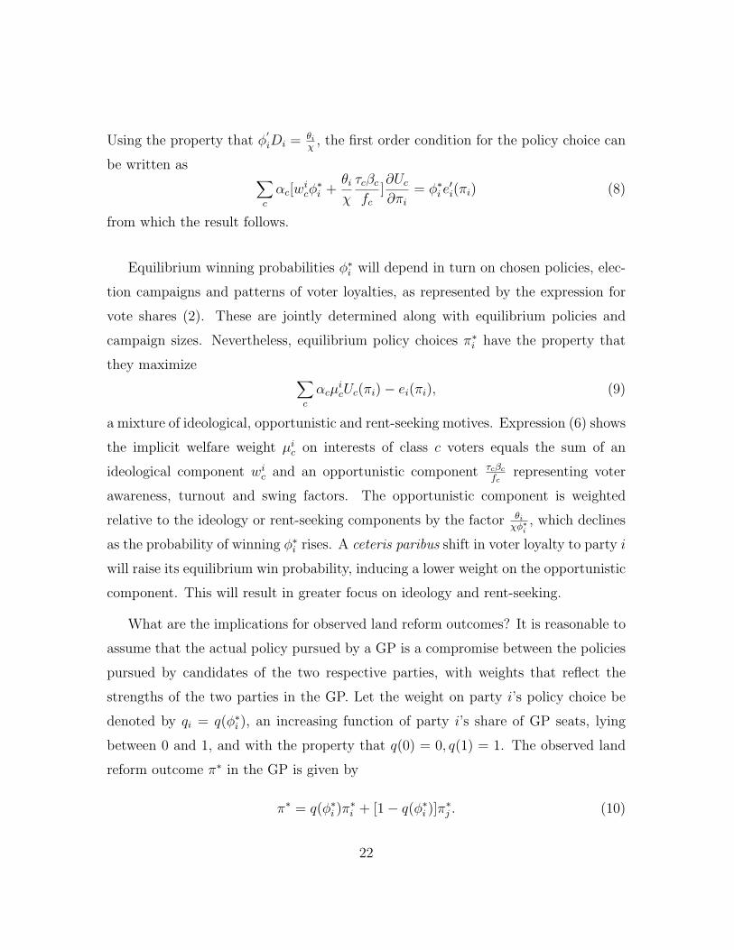
What are the implications for observed land reform outcomes? It is reasonable to

assume that the actual policy pursued by a GP is a compromise between the policies

pursued by candidates of the two respective parties, with weights that reflect the

strengths of the two parties in the GP. Let the weight on party i’s policy choice be

denoted by qi = q(φ∗i ), an increasing function of party i’s share of GP seats, lying

between 0 and 1, and with the property that q(0) = 0, q(1) = 1. The observed land

reform outcome π∗ in the GP is given by

π∗ = q(φ∗i )π

∗i + [1 − q(φ∗

i )]π∗j . (10)

22

Let πIi denote the ideal policy for party i which it would pursue in the absence

of any opportunistic motive, i.e., which maximizes∑

c αcwicUc(π) − e(π). And let

πD denote the Downsian equilibrium policy outcome, which maximizes∑

c αcτc

fcUc(π).

Note that the Downsian policy does not incorporate the personal rents of elected

officials. If the extent of land reform π is a one dimensional variable then for reasons

explained above one would expect e(π) to be an increasing function. Then the extent

of land reform will tend to be underprovided as a result of the political moral hazard

problem. This will be mitigated only if party i has a sufficient ideological preference

for the reform.

Consider the case where the political moral hazard problem dominates ideological

considerations, in the sense that the Downsian policy πD strictly exceeds the ideal

policy πIi of both parties i = L, R. This is illustrated in Figure 1. Call this Case 1

from now on. Here a rise in its win probability causes the equilibrium policy of the

Left to move closer to its own desired policy πIL, i.e., it carries out less land reform.

At the same time the Right party will implement more land reform in order to recover

ground with voters. If the Left party was carrying out more land reform initially, the

gap between the two parties will narrow. As voters continue to shift loyalty to the

Left party, eventually the gap will vanish and then get reversed, with the Right party

carrying out more land reform than the Left.22

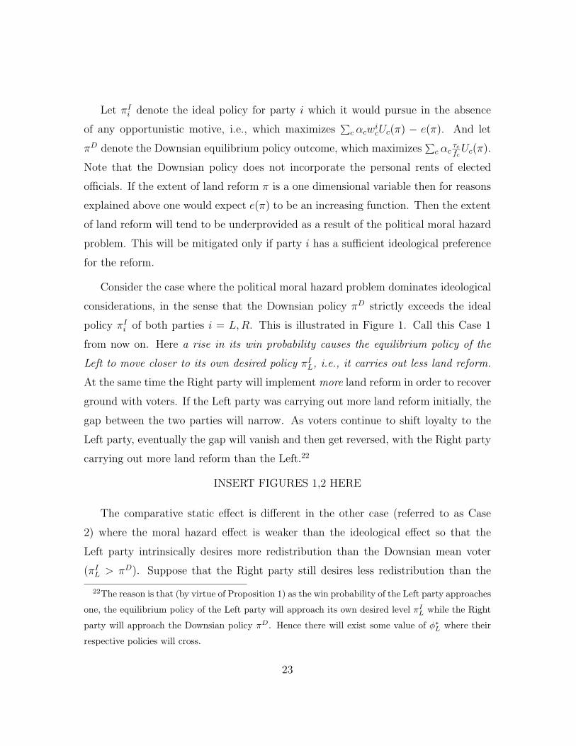
INSERT FIGURES 1,2 HERE

The comparative static effect is different in the other case (referred to as Case

2) where the moral hazard effect is weaker than the ideological effect so that the

Left party intrinsically desires more redistribution than the Downsian mean voter

(πIL > πD). Suppose that the Right party still desires less redistribution than the

22The reason is that (by virtue of Proposition 1) as the win probability of the Left party approaches

one, the equilibrium policy of the Left party will approach its own desired level πIL while the Right

party will approach the Downsian policy πD. Hence there will exist some value of φ∗L where their

respective policies will cross.

23

Downsian outcome. Then an increase in its win probability motivates the Left party

to carry out more redistribution. The Right party also wishes to carry out more

redistribution. In this case both parties carry out more land reform with a shift in

voter loyalty to the Left, as illustrated in Figure 2. Moreover here the Left party will

always carry out more redistribution than the Right party (since the Left will always

want to carry out more than the Downsian policy, and the Right party less than the

Downsian policy). In this case the results will be akin to the pure ideology model:

there will be a monotone, increasing relationship between Left share of GP seats and

the extent of land reform.

4 Testing the Model

The first step in empirical testing is to incorporate possible endogeneity of the Left

share. Unobserved determinants of citizen preferences for land reform could be corre-

lated with loyalties to the Left Front alliance. Normally one would expect that these

would be positively correlated, in which case the bias in estimating the coefficient is

positive. The absence of a positive observed relation of land reform with Left share

would be consistent with the pure ideology hypothesis only if unobserved preferences

for land reform were negatively correlated with the success of the Left Front. This

seems rather far-fetched, given the stated ideology and constituencies represented by

the two parties. Nevertheless, just to be sure, we need to obtain instruments for the

Left share.

4.1 Predicting Success of the Left in Local Elections

Probabilistic voting models allow voting behavior to reflect both loyalties of voters to

different parties for various exogenous reasons (such as historical factors, incumbency,

the specific characteristics of candidates etc.), as well as their policy preferences. We

24

can therefore search for determinants of voter loyalty to the Left that reflect factors

external to the village, or historical circumstances orthogonal to issues affecting the

current election. The Left and Congress contest elections at various different levels

above the GP, such as the state and federal legislatures (which we shall henceforth

refer to as the Assembly and Parliament respectively). These elections are staggered

across different years: the Assembly elections are typically held one or two years

before the GP elections (they were held in 1977, 1982, 1987, 1991 and 1996). The

Left and the Congress were the principal adversaries in the state assembly elections,

as well as elections for seats representing West Bengal constituencies in the national

Parliament (Lok Sabha).

Given that local government elections were introduced for the first time in 1978,

and that most voters in India tend to view politics in terms of state or national rather

than local issues, it is plausible to suppose that voter loyalties to the two rival parties

in local elections were determined to a considerable extent by regional or national

issues. These are proxied by the relative strength of the two parties in the national

Parliament. The Congress formed the national government between 1980 and 1984,

and reinforced its position between 1984 and 1989 following the assassination of Indira

Gandhi in 1984. Between 1989 and 1991 a non-Congress government prevailed at the

national level, representing a coalition of different regional parties supported by the

West Bengal Left Front. Then again from 1991 until 1996 the Congress formed a

government at the national level, with the Left in the opposition.

The fluctuating strength of the two parties in Parliament had considerable impli-

cations for relations between the central and the state government over fiscal trans-

fers, execution of central government projects in the state, and other matters likely

to have significant spillovers into inflation, employment and public services. The

Congress party can obtain an advantage in local elections from shifts in voter loyalty

towards the Congress in general owing to national events. Conversely, Left candidates

can blame a Congress-inclusive coalition central government for starving the state of

25

fiscal transfers or public investments, and use this in their election rhetoric in order

to mobilize voters against the Congress party.

Table 7 presents regressions predicting Left control of local GPs, on the basis of a

variety of factors both external and internal to the villages in question. The external

factors include the proportion of seats secured by the Congress in the currently elected

(national) Parliament. We also include the average vote share difference (AVSD,

hereafter) between Left and Congress candidates in the immediately preceding state

Assembly elections, averaged at the district level, as a proxy for prevailing voter

loyalty to the two parties on the basis of district, state or national issues. State

assembly elections are held every five years but interspersed with elections to local

governments. There is typically a two or three year period separating Assembly

elections and GP elections. The AVSD from the last state Assembly election usually

provides a signal of the competitive strength of the two parties in the nearest Assembly

constituency. To remove the influence of issues concerning the local area in which a

GP is located, we average the AVSD across all constituencies in the district.23

Local factors that may affect electoral success of the Left in GP elections include

incumbency patterns in the GP, besides land distribution, literacy and caste in the

village. The regressions interact local incumbency with the share of the Congress

in national Parliament seats, since (as argued above) voters reaction to changes in

national politics are likely to depend on which party dominates the local area.

Table 7 shows results of the GP Left share regression applied to five successive

GP elections (1978, 1983, 1988, 1993 and 1998). The regressions control for village

land distribution, illiteracy rate among landless, marginal and small landowners, and

proportion of households in scheduled castes and tribes. The first column shows cross-

section least squares results, while the remaining three show the panel estimates

(which include village dummies). In the panel we use the Arellano-Bond (1991)

23There are approximately twenty assembly constituencies (and 200 GPs) per district.

26

estimator to avoid the bias that arises from a lagged dependent variable (incumbency,

i.e., Left share in the previous GP election) as a regressor. The hypothesis of lack of

first-order serial correlation in the time-varying errors (equivalently lack of second-

order correlation in the differenced residuals) is not rejected (the p-value of the test

is 0.77).

The cross-section regression shows that the assembly vote share difference at the

district level was a strong predictor of local GP outcomes. The panel regressions

in the remaining columns of Table 7 replace or augment the district voter loyalty

variable with its underlying determinants. The second and third columns show that

changing fortunes of the Left in GP elections (conditional on incumbency patterns)

were predicted by changes in national politics — the presence of Congress in national

Parliament — rather than changes in village characteristics.24 The nature of this

dependence is intuitively plausible: rising Congress fortunes at the national level

helped the Congress in GP elections in constituencies where they were already strong.

A rise in the presence of the Congress at the national level also benefited the Left

party in areas where the Left was traditionally powerful. This probably reflects ability

of the Left to gain mileage with voters by blaming a Congress-dominated national

government for local problems. The last column of Table 7 shows that even after

controlling for these factors, the district level vote share difference in the previous

Assembly elections remains significant as a determinant of Left share in the GP

election. Conversely, controlling for the state assembly vote share difference, the

presence of the Congress in national Parliament interacted with local incumbency

patterns continue to be a significant predictor of GP election outcomes

24Inclusion of lagged land reform in the village concerned on the right hand side did not yield a

significant coefficient either, irrespective of whether it was included by itself or in interaction with

incumbency.

27

4.2 Instrumental Variable Estimates of the Land Reform-

Left GP share relationship

The preceding results suggest that external and historical factors driving the fluctua-

tions in Left control of local GPs could be used as instruments to correct for potential

endogeneity of the Left share variable in the land reform regression. This requires the

assumption that these factors were unrelated to village-specific time-varying factors

affecting land reforms, after controlling for their effects on GP election outcomes.

This assumption seems credible for the presence of Congress in the national Par-

liament. This variable reflects the growing importance of coalition politics at the

national level, and other events in the rest of the country.25 Added to this the fact

that West Bengal accounts for only 42 out of 540 seats in the national Parliament,

and that most seats secured by the Congress in Parliament were from other states,

the likelihood of reverse causality is quite remote.

The exclusion restriction requires that the instruments: changes in Congress pres-

ence in national Parliament in conjunction with lagged Left share of GP seats, were

uncorrelated with unobserved determinants of year-to-year changes in land reform

implemented in villages, after controlling for village and time dummies and local dis-

tribution of land, caste and literacy. Congress presence in national Parliament could

of course affect macroeconomic variables such as inflation and unemployment which

in turn could affect poverty and income distribution in villages, and hence the po-

litical demand for land reform. They could also affect fiscal transfers to the state of

West Bengal and investment projects funded by the Central government. But these

would affect all villages within West Bengal in the same way, and would therefore be

picked up by the time dummies.26

25These include seccessionist movements in Punjab and Kashmir, the assassinations of Indira

Gandhi and Rajiv Gandhi which subsequently created a pro-Congress wave, rising power of regional

parties and the Bharatiya Janata Party in other parts of India, and border tensions with Pakistan.26Transfers to local governments are made by the state government, and central government

28

Moreover, Table 7 shows we cannot reject the hypothesis of absence of serial corre-

lation in the Left share regression after controlling for village fixed effects. Combined

with the assumption of zero serial correlation in unobservables in both land reform

Left share regressions after controlling for village and time dummies, incumbency

(lagged Left share) also satisfies the exclusion restriction.27

Accordingly, we use the second column of Table 7 to predict the Left share in

each GP, and then use these in a second-stage instrumental variable land reform-Left

share regression.28

4.3 Regression Specification

We now describe the regression specification implied by the theory. Recall equation

(10) which generates the land reform outcome in any village as a function of the Left

share of the GP, and the policies pursued by the two parties. For village v in year t:

πvt = q(LSvt)(πLvt − πR

vt) + πRvt (11)

where we use a quadratic formulation q(l) ≡ al + bl2, l ∈ [0, 1] for Left control.

The Left share of GP seats is jointly determined along with the policies chosen

by the two parties, besides determinants of voter loyalties. Shifting voter loyalties

also affect equilibrium policy choices in the model, by affecting relative competitive

transfers are routed through the state government. The national government thus has little discretion

to alter allocation of transfers across local governments within any given state. It is therefore unlikely

that changes in the role of Congress in the national government would affect resource transfers or

investment projects to different villages within West Bengal differently.27In other words, the assumption is that the village fixed effects soak up all the serial correlation in

unobserved factors, in both the Left share and land reform regressions. This was empirically verified

in the case of the Left share regression. Note that no restriction is needed for contemporaneous

correlation of time-varying unobservables across the two equations.28The correlation between the predicted and observed changes was .32.

29

strength of the two parties. Recall that policies are chosen by elected officials in

a given administration partly with an eye to their re-election prospects in the next

election. Hence the implicit welfare weights in (6) are based on the best estimate

available to the officials of their win probability in the next election. Let LDvt denote a

signal available to parties concerning voter loyalty to the Left relative to the Congress.

Also let Svt denote a vector of distributional characteristics pertaining to land, literacy

and caste in village v in year t. The policy of the Right party can then be represented

by

πRvt = λ0 + λ1LDvt + λ2Svt + ηR

vt (12)

and the divergence in policies between the two parties by

πLvt − πR

vt = μ0 + μ1LDvt + μ2Svt + ηdvt, (13)

where ηRvt, η

dvt denote regression residuals.

Combining the policy equations with (11), we obtain the following prediction for

land reform:

πvt = λ0 + λ1LDvt + λ2Svt +

+ μ0q(LSvt) + μ1LDvt ∗ q(LSvt) + μ2Svt ∗ q(LSvt) + ηvt (14)

The coefficient μ1 represents the interaction between moral hazard and competition

missing in the pure Downsian and ideology models. The Downsian model predicts no

policy divergence (μ0 = μ1 = μ2 = 0) and irrelevance of voter loyalties (λ1 = 0). The

pure ideology model also implies irrelevance of voter loyalties (μ1 = λ1 = 0), while

policy divergence is predicted (μ0 �= 0, μ2 �= 0). The hybrid model predicts that voter

loyalties matter for policy. If political moral hazard is severe enough in the sense

explained in the previous section, λ1 > 0, μ1 < 0.

Note that in the presence of significant interactions between moral hazard and

competition, the land reform regression estimated previously was misspecified. The

interaction effects are correlated with the Left share variable, causing the estimated

30

coefficient of q(LSvt) to be biased. The sign of this bias depends on the sign of the

interaction effect. If Case 1 applies, the moral hazard-competition interaction causes

policy divergence to narrow and get reversed when voters shift loyalty to the Left,

causing a downward bias in the estimated coefficient μ0.

4.4 Empirical Results

To operationalize this approach, we need a variable representing LDvt, a measure of

relative voter loyalties to the Left available to elected officials prior to the election.

One possible proxy is AV SDvt, the average vote share difference between the two

parties in the preceding state Assembly elections in the local area. Another is LSvt,

the proportion of seats secured by the Left in the local GP in the preceding panchayat

election. Either or both of these could be used. We prefer to use the former, the

Assembly vote share difference, for a number of reasons. First, with state Assembly

elections held halfway between panchayat elections, the most recent Assembly results

provide a more up-to-date signal of voter loyalties for at least the second half of

the current GP administration. In addition, the interaction term can be simply

interpreted: as the extent to which rising competitive strength within a broader area

and context (the district assembly elections) motivates a slackening of land reform

effort. Second, using LSvt would imply that the key interaction between q(LSvt)

would reduce to a higher-order term involving LSvt. This interaction would then be

difficult to distinguish from (a higher-order term in a polynomial approximation to)

the effect of Left control of the local GP represented by q(LSvt).29

One useful indication of pressures of electoral competition is the presence of spikes

29It is difficult to know for sure the exact nature of non-linearity of q(.), i.e., the way that the

control of the GP varies with the Left share of seats. Moreover, if q(.) is represented by a quadratic,

the interaction term would reduce to a cubic term in LSvt, which would also raise multicollinearity

problems and reduce statistical precision.

31

of reform effort in periods immediately preceding elections. Such spikes are difficult

to reconcile with the intrinsic policy preferences or ideological concerns. We shall

therefore run the regression on data at the village-year level, adding dummies for

election and pre-election years. In order to identify these, we cannot use year dum-

mies. We therefore use timeblock dummies (each corresponding to a five year GP

administration) in conjunction with election-year and pre-election year dummies, in

order to capture macroeconomic effects and those associated with a given elected GP

administration.30

This compounds the problem of censoring in the data. Table 5 indicated that

in most five-year timeblocks, upwards of two-thirds of all villages did not carry out

any titling or tenancy registration at all. The extent of censoring is even higher

when the data is organized at the yearly level: upwards of 1500 village years out of

a total of 1740 witnessed no patta distribution or tenancy registration. Accordingly,

the regression ought to incorporate endogenous censoring, which is challenging in

the context of panel data (since the resulting nonlinearity of the model implies that

village dummies cannot be ‘washed out’ by taking inter-year deviations for any given

village).

In what follows we deal with the censoring problem as follows. First we esti-

mate the tobit version of the regression, using the semiparametric trimmed LAD

estimator with village fixed effects proposed by Honore (1992). Besides controlling

for inter-village heterogeneity and censoring, the latter estimator avoids the normality

assumption on residuals, replacing it with only a symmetry (i.i.d.) restriction on the

distribution of time-varying residuals.

Tables 8 through 11 present the linear-IV and censored TLAD land reform regres-

sions with and without instrumental variables. The TLAD specification takes the

30Alternatively, year dummies can be used but then election timing effects cannot be estimated.

We have also run the regressions with year dummies and obtained similar results. The results for

these regressions are available on request.

32

form 31

πvt = max[0, μ0q(LSvt)+μ1AV SDvt∗q(LSvt)+λ1AV SDvt+λ2Svt+λv+δT (t)+θ1DPt+θ2DEt+ηvt]

(15)

with the linear specification being the corresponding uncensored version, where DPt, DEt

denote pre-election and election year dummies, T (t) denotes the time-block corre-

sponding to a given GP administration, and ηvt is an i.i.d. error term. Both versions

with observed and predicted (i.e., instrumented) Left shares are shown for the TLAD

estimates. As explained previously, the instruments for Left share include local in-

cumbency (lagged Left share of GP seats), the presence of Congress in the national

Parliament, and interactions between these. The predicted Left shares are generated

from column 2 in Table 7. We also instrument the interactions between AVSD and

Left share and its square, by the interactions between AVSD and predicted values

and squares of the Left share.

Standard errors are clustered at the district level, and in the IV regressions are

reported both with and without bootstrapping. To correct for possible serial correla-

tion in the residuals for any given village not captured by village fixed effects, we use

a block bootstrap as recommended by Bertrand, Duflo and Mullainathan (2004).32

Controls included in Svt include interpolated (i.e., village-specific time trends in) area

and population shares in different landownership size-classes, illiteracy rates among

households owning less than 5 acres of non-patta land, the proportion of households

belonging to scheduled castes and tribes. In addition the regression includes dummies

31For the sake of parsimony and limiting multicollinearity, we drop interactions between q(LSvt)

and Svt.32Specifically, all the data for a given district is kept as a single block, and 200 samples are

generated by sampling with replacement from the blocks in a way that yields between 90 and 100

villages in each sample. (There are 15 districts, each containing between two to eight villages, as

shown in Table 1). Both first stage and second stage regressions are run for each sample, so that the

bootstrapped standard errors incorporate first stage prediction errors as well as serial correlation

and clustering of residuals.

33

for different timeblocks, villages and election/pre-election years.33

We report the regression results for two different time spans. Tables 8 and 9

pertain to titling and sharecropped registration over the 1978-98 period, spanning

four successive elected GP administrations. Tables 10 and 11 pertain to the period

1974-98, adding the period 1974-78 when GPs had not yet been created and land

reforms were implemented at the behest of the state government which was dominated

by the Congress. We accordingly put the Left share during the pre-1978 period at

zero. This longer time span enables us to add observations from a period when the

implementing agency was controlled by the Congress rather than the Left Front. As

it turns out, this adds considerably to the statistical precision of the results.

Tables 8 through 11 show that the signs and magnitudes of the TLAD coefficients

of Left share, its square and interactions of these with average vote share difference

(AVSD) in preceding Assembly elections are consistent with the predictions of the

theory for Case 1, where the competition-moral hazard interaction effect outweighs

the idelology effect.34 For this case the theory predicts the coefficient of Left share to

be positive and its square to be negative, with an opposite pattern for the respective

interactions with AVSD. Implied turning points for the quadratic in the Left-share

itself and implicit in the interaction of this with average voter loyalty are reported at

the bottom of each column. The theory predicts these two turning points will be the

same, which is seen to borne out reasonably well in the TLAD regressions.

33It could be argued that the regression should additionally include measures of land reform

implemented in the past, as this affects the residual capacity for further reform. We avoid this

owing to the well-known econometric problems associated with lagged dependent variables, apart

from the fact that in the case of the titling program there seems to continue to be a large surplus of

vested land that still remains to be distributed, which implies that ‘capacity constraints’ ought not

to matter.34The single exception is the 1978-98 TLAD IV regression for proportion of land titled, in which

implementation is decreasing in Left share. Even in this case, the evidence is unfavorable for the

ideology hypothesis.

34

However, when the sample is restricted to the 1978-98 period, most of the relevant

coefficients are imprecisely estimated, as the standard errors are large. The precisions

are higher in Tables 10 and 11 which are based on the 1974-78 period. This is

particularly so in case of the land titling program, where interaction effects of Left

share and its square with AVSD remain significant at the 5% level after adjusting

for censoring, endogeneity and bootstrapping standard errors to control for clustering

and serial correlation of residuals. In addition, we see significant spikes in pre-election

years for the propotion of land titled in all three regressions in Table 10. The results

are less precise for tenancy registration, with the exception of significant election

year spikes in proportion of households registered, and a significant (at 10%) increase

in implementation in Congress-dominated villages when voter loyalties (indicated by

vote shares in the preceding Assembly election) swung in favor of the Left.

The corresponding coefficients of other village characteristics in the regressions in

Tables 8-9 are shown in Table 12. The proportion of households receiving land titles

was higher when there were more marginal landowners, fewer medium landowners, a

smaller fraction of non-patta land was in small holdings below 5 acres, and the poor

(landless or marginal landowners) were less illiterate. This is consistent with the

notion that the titling program was responsive to voter preferences and awareness, as

postulated by the Downsian theory. Medium landowners are likely to have been the

most politically active groups opposing the land reform, as giving land to the poor

would raise the self-sufficiency of the latter, reducing their willingness to work for low

wages on the farms of landowners, and their dependence on the latter for informal

credit. Large landowners would have the same (or greater) interest in blocking the

reforms, but they lost most of their political clout after the Left coalition gained

power at both the state and local levels since 1978.35 The group most likely to be

active in pushing for the reforms would be marginal landowners, and they would be

35See Bhattacharya (1999) for ground-level evidence of the Left Front being captured by medium

farmers.

35

politically more effective if they were more literate. And they would be able to make

a stronger case for the reforms if the local land distribution was more skewed against

small holdings. An increase in the proportion of low caste households (who tend to

be poorer than the average household) also reduced the proportion of land reformed,

but this is significant only when standard errors are not bootstrapped.

5 Concluding Comments

In summary, we find no evidence supporting the hypothesis that land reform im-

plementation in West Bengal since the 1970s was driven simply by the extent of

control exercised by the Left-front coalition over local governments. Instead it is

consistent with Downsian or quasi-Downsian theories which stress the importance of

electoral opportunism and competition. The point estimates are consistent with the

quasi-Downsian theory predicting an inverted-U pattern between land reform and

Left share of seats in the local government, and a negative interaction between Left

share and voter loyalty towards the Left. In other words, the Left was less inclined

to implement the reforms when its control over local governments increased beyond

an absolute majority (which was mostly the case). This was accentuated when the

Left was in a stronger competitive position, as indicated by an increase in their vote

share in preceding state assembly elections in the district in question.

However, the statistical precision of these estimates are unreliable and depend on

the exact dependent variable, specification and time-period studied. If on this basis

we were to conclude that the evidence for the inverted-U pattern is not robust, we

would be inclined to view the evidence as indicating the absence of any significant re-

lationship between land reform implementation and Left control of local governments.

In other words, we would see this as evidence in favor of the pure Downsian theory

vis-a-vis the quasi-Downsian theory. We find no evidence of a monotonic positive

association between Left share of local governments and land reforms implemented,

36

as the ideology model predicts. The role of electoral competition is further indicated

by the significant spikes observed in election or pre-election years.

A number of caveats are in order. The Left Front undoubtedly played a significant

role at the level of the state government by putting land reform on the forefront

of their agenda for agrarian reform in the state. There is no doubt West Bengal

achieved significantly more compared with most other Indian states with regard to

implementing land reforms. Our results pertain only to the role of officials elected

to local governments, and may therefore reflect problems of agency between the Left

Front and the candidates they nominated to elections to local governments.

Alternative explanations to moral hazard or rent-seeking on the part of elected

officials may be provided for their reluctance to implement much land reform when

they are in a strong competitive position.36 For instance, it is possible that they per-

ceive a given stock of land reform that can be implemented between the current and

future, defined by the amount of vested land or the extent of land under tenancy yet

to be registered. They may want to hold back on the amount currently implemented,

so as to leave more available for the future when they are in a weaker competitive po-

sition compared to the current period. We have no way of discriminating empirically

between this theory and the one we have offered in the paper.

The results of this paper indicate the relative importance of electoral competition

and ideology or policy preferences of elected officials. Our results pertain to the

context of land reforms implemented in West Bengal in a specific time period. Studies

pertaining to other countries, regions or programs are needed before we can draw any

general inferences.

36We thank Saumitra Jha for this observation.

37

References

Arellano M. and S. Bond (1991), ‘Some Tests of Specification for Panel Data:

Monte Carlo Evidence and an Application to Employment Equations’, Review

of Economic Studies 58, 277-297.

Appu P.S. (1996), Land Reforms in India, Delhi: Vikas Publishing House.

Bandyopadhyay D. (1986), ‘Land Reforms in India: An Analysis,” Economic and

Political Weekly, XXI, 25/26: A50-A56.

Banerjee A., P. Gertler, and M. Ghatak (2002), Empowerment and Efficiency:

Tenancy Reform in West Bengal, Journal of Political Economy, 110(2), 239-

280.

Bardhan P. (1973), “Size, Productivity and Returns to Scale: An Analysis of

Farm-Level Data in Indian Agriculture,” Journal of Political Economy, 81(6),

1370–86.

Bardhan P. and D. Mookherjee (2004), “Pro-Poor Targeting and Accountabil-

ity of Local Elections in West Bengal,” forthcoming, Journal of Development

Economics.

Basu S.K. and S.K. Bhattacharya (1963), Land Reforms in West Bengal: A Study

on Implementation, Calcutta: Oxford Book Company.

Bell C. (1977), “Alternative Theories of Sharecropping: Some Tests Using Evidence

from Northeast India,” Journal of Development Studies, 13(4), 317–346.

Bergmann T. (1984), Agrarian Reform in India, with Special Reference to Kerala,

Karnataka, Andhra Pradesh and West Bengal. New Delhi: Agricole.

Berry A. and Cline W. (1979), Agrarian Structure and Productivity in Developing

Countries, Baltimore: Johns Hopkins University Press.

38

Bertrand M., E. Duflo and S. Mullainathan (2004), “How Much Should We Trust

Differences-in-Differences Estimates?” Quarterly Journal of Economics, Febru-

ary 2004, 249–275.

Besley T. and Burgess R. (2000) “Land Reform, Poverty Reduction and Growth:

Evidence from India,” Quarterly Journal of Economics 115, no. 2, 389-430.

Binswanger H., Deininger K., and Feder G. (1993), “Power, Distortions, Revolt

and Reform in Agricultural Land Relations,” in J. Behrman and T.N. Srinivasan

(Ed.), Handbook of Development Economics, vol. III, Amsterdam: Elsevier.

Binswanger H. and M. Rosenzweig (1993), “Wealth, Weather Risk and the Compo-

sition and Profitability of Agricultural Investments,” Economic Journal, 56-78.

Bhattacharya, D. (1999), ‘Politics of Middleness: The Changing Character of the

Communist Party of India (Marxist) in Rural Bengal (1977-90),’ in B. Ro-

galy, B. Harriss-White and S. Bose (Ed.), Sonar Bangla? Agricultural Growth

and Agrarian Change in West Bengal and Bangladesh, Sage Publications., New

Delhi and Thousand Oaks, London.

Case A. (2001), “Election Goals and Income Redistribution: Recent Evidence From

Albania,” European Economic Review, 45, 405-423.

Chatterjee P. (1984), Bengal 1920-47: The Land Question, Calcutta: K.P. Bagchi.

Cooper A. (1988), Sharecropping and Sharecroppers’ Struggles in Bengal, Calcutta:

K.P. Bagchi and Co.

Dixit A. and J. Londregan (1998), “Ideology, Tactics and Efficiency in Redistribu-

tive Politics,” Quarterly Journal of Economics, May 1998, 497–529.

Donald S. and K. Lang (2004), “Inference with Difference in Differences and Other

Panel Data,” mimeo, Department of Economics, Boston University.

39

Downs A. (1957), An Economic Theory of Democracy, New York: HarperCollins.

Franda M. (1971), Radical Politics in West Bengal, Cambridge, MA: MIT Press.

Grossman G. and Elhanan Helpman, “Electoral Competition and Special Interest

Politics,” Review of Economic Studies, 63, 265-286, 1996.

Honore B. (1992), ‘Trimmed LAD and Least Squares Estimation of Truncated and

Censored Regression Models with Fixed Effects,’ Econometrica, 60, 533-565.

Kohli A. (1987), State of Poverty in India, Cambridge: Cambridge University

Press.

Lieten G.K. (1992), Continuity and Change in Rural West Bengal, New Delhi:

Sage Publications.

Lindbeck A. and J. Weibull (1993), “A Model of Political Equilibrium in a Repre-

sentative Democracy,” Journal of Public Economics, 51, 195–209.

Lipset S.M. (1960), Political Man. Baltimore: Johns Hopkins University Press.

Nossiter T.J. (1988), Marxist State Governments in India, London: Pinter Pub-

lishers.

Rogaly B., B. Harriss-White and S. Bose (Ed.) (1999), Sonar Bangla? Agri-

cultural Growth and Agrarian Change in West Bengal and Bangladesh, Sage

Publications, New Delhi and Thousand Oaks, London.

Sengupta S. (1981), ‘West Bengal Land Reforms and the Agrarian Scene,” Eco-

nomic and Political Weekly, XVI, 25/26: A26-A75.

Webster N. (1992), Panchayati Raj and the Decentralisation of Development Plan-

ning in West Bengal, Calcutta: K.P. Bagchi and Co.

40

Wittman D. (1973), ‘Parties as Utility Maximizers,” American Political Science

Review, 67, 490–498.

41

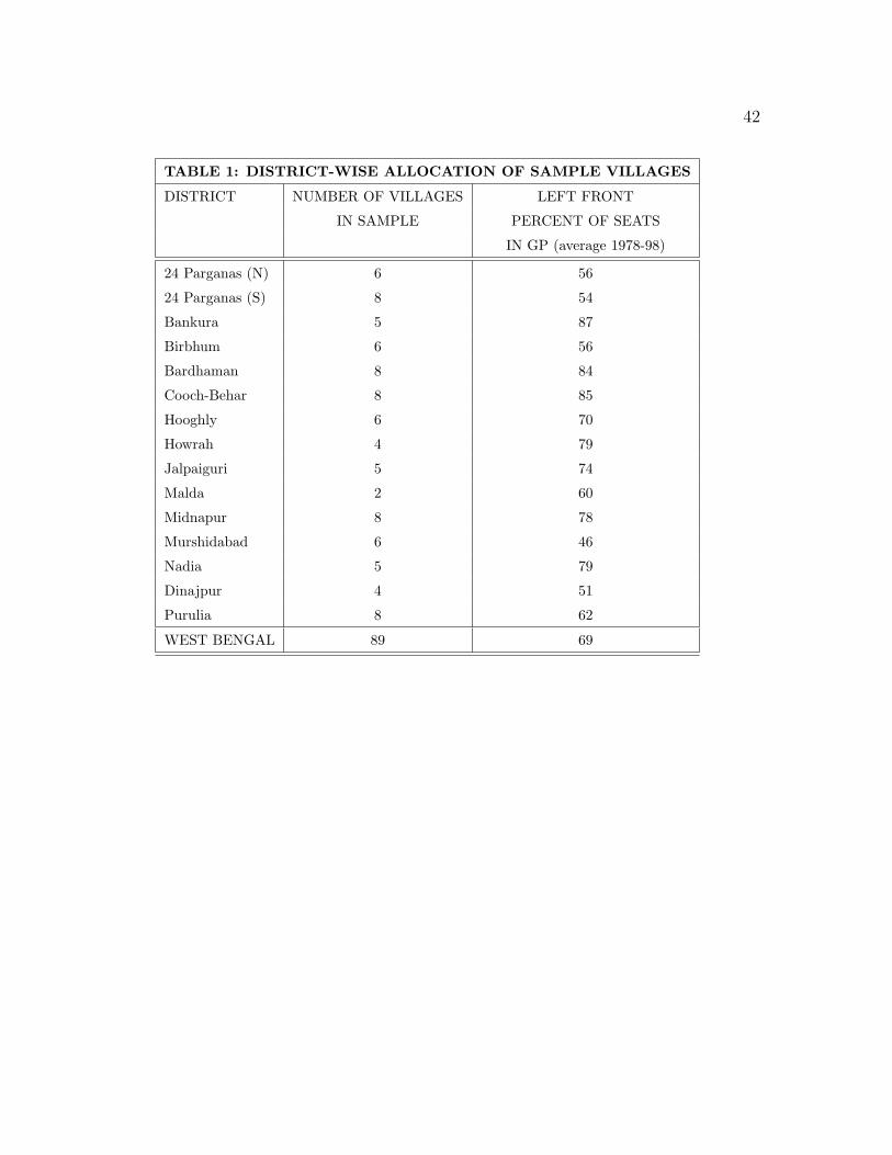
42

TABLE 1: DISTRICT-WISE ALLOCATION OF SAMPLE VILLAGES

DISTRICT NUMBER OF VILLAGES LEFT FRONT

IN SAMPLE PERCENT OF SEATS

IN GP (average 1978-98)

24 Parganas (N) 6 56

24 Parganas (S) 8 54

Bankura 5 87

Birbhum 6 56

Bardhaman 8 84

Cooch-Behar 8 85

Hooghly 6 70

Howrah 4 79

Jalpaiguri 5 74

Malda 2 60

Midnapur 8 78

Murshidabad 6 46

Nadia 5 79

Dinajpur 4 51

Purulia 8 62

WEST BENGAL 89 69

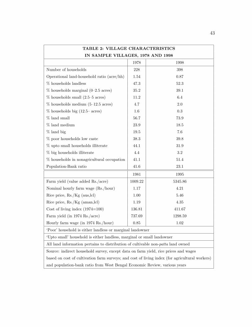
43

TABLE 2: VILLAGE CHARACTERISTICS

IN SAMPLE VILLAGES, 1978 AND 1998

1978 1998

Number of households 228 398

Operational land-household ratio (acre/hh) 1.54 0.87

% households landless 47.3 52.3

% households marginal (0–2.5 acres) 35.2 39.1

% households small (2.5–5 acres) 11.2 6.4

% households medium (5–12.5 acres) 4.7 2.0

% households big (12.5– acres) 1.6 0.3

% land small 56.7 73.9

% land medium 23.9 18.5

% land big 19.5 7.6

% poor households low caste 38.3 39.8

% upto small households illiterate 44.1 31.9

% big households illiterate 4.4 3.2

% households in nonagricultural occupation 41.1 51.4

Population-Bank ratio 41.6 23.1

1981 1995

Farm yield (value added Rs./acre) 1009.22 5345.86

Nominal hourly farm wage (Rs./hour) 1.17 4.21

Rice price, Rs./Kg (aus,lcl) 1.00 5.46

Rice price, Rs./Kg (aman,lcl) 1.19 4.35

Cost of living index (1974=100) 136.81 411.67

Farm yield (in 1974 Rs./acre) 737.69 1298.59

Hourly farm wage (in 1974 Rs./hour) 0.85 1.02

‘Poor’ household is either landless or marginal landowner

‘Upto small’ household is either landless, marginal or small landowner

All land information pertains to distribution of cultivable non-patta land owned

Source: indirect household survey, except data on farm yield, rice prices and wages

based on cost of cultivation farm surveys; and cost of living index (for agricultural workers)

and population-bank ratio from West Bengal Economic Review, various years

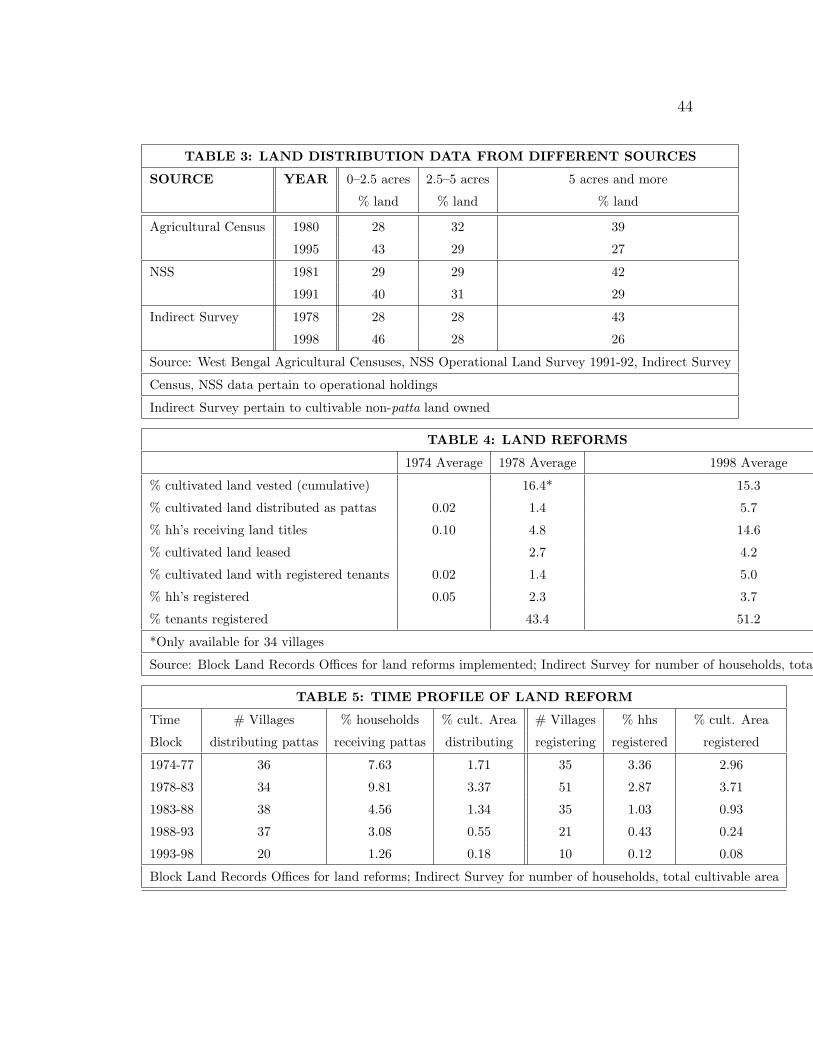
44

TABLE 3: LAND DISTRIBUTION DATA FROM DIFFERENT SOURCES

SOURCE YEAR 0–2.5 acres 2.5–5 acres 5 acres and more

% land % land % land

Agricultural Census 1980 28 32 39

1995 43 29 27

NSS 1981 29 29 42

1991 40 31 29

Indirect Survey 1978 28 28 43

1998 46 28 26

Source: West Bengal Agricultural Censuses, NSS Operational Land Survey 1991-92, Indirect Survey

Census, NSS data pertain to operational holdings

Indirect Survey pertain to cultivable non-patta land owned

TABLE 4: LAND REFORMS

1974 Average 1978 Average 1998 Average

% cultivated land vested (cumulative) 16.4* 15.3

% cultivated land distributed as pattas 0.02 1.4 5.7

% hh’s receiving land titles 0.10 4.8 14.6

% cultivated land leased 2.7 4.2

% cultivated land with registered tenants 0.02 1.4 5.0

% hh’s registered 0.05 2.3 3.7

% tenants registered 43.4 51.2

*Only available for 34 villages

Source: Block Land Records Offices for land reforms implemented; Indirect Survey for number of households, total

TABLE 5: TIME PROFILE OF LAND REFORM

Time # Villages % households % cult. Area # Villages % hhs % cult. Area

Block distributing pattas receiving pattas distributing registering registered registered

1974-77 36 7.63 1.71 35 3.36 2.96

1978-83 34 9.81 3.37 51 2.87 3.71

1983-88 38 4.56 1.34 35 1.03 0.93

1988-93 37 3.08 0.55 21 0.43 0.24

1993-98 20 1.26 0.18 10 0.12 0.08

Block Land Records Offices for land reforms; Indirect Survey for number of households, total cultivable area

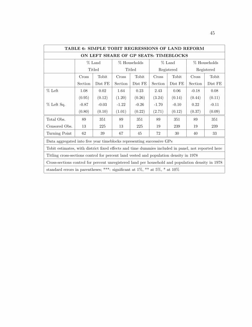
45

TABLE 6: SIMPLE TOBIT REGRESSIONS OF LAND REFORM

ON LEFT SHARE OF GP SEATS: TIMEBLOCKS

% Land % Households % Land % Households

Titled Titled Registered Registered

Cross Tobit Cross Tobit Cross Tobit Cross Tobit

Section Dist FE Section Dist FE Section Dist FE Section Dist FE

% Left 1.08 0.02 1.64 0.23 2.43 0.06 -0.18 0.08

(0.95) (0.12) (1.20) (0.26) (3.24) (0.14) (0.44) (0.11)

% Left Sq. -0.87 -0.03 -1.22 -0.26 -1.70 -0.10 0.22 -0.11

(0.80) (0.10) (1.01) (0.22) (2.71) (0.12) (0.37) (0.09)

Total Obs. 89 351 89 351 89 351 89 351

Censored Obs. 13 225 13 225 19 239 19 239

Turning Point 62 39 67 45 72 30 40 33

Data aggregated into five year timeblocks representing successive GPs

Tobit estimates, with district fixed effects and time dummies included in panel, not reported here

Titling cross-sections control for percent land vested and population density in 1978

Cross-sections control for percent unregistered land per household and population density in 1978

standard errors in parentheses; ***: significant at 1%, ** at 5%, * at 10%

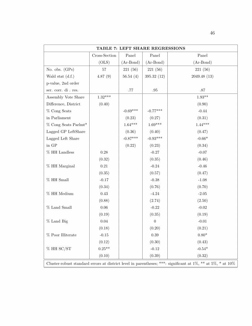
46

TABLE 7: LEFT SHARE REGRESSIONS

Cross-Section Panel Panel Panel

(OLS) (Ar-Bond) (Ar-Bond) (Ar-Bond)

No. obs. (GPs) 57 221 (56) 221 (56) 221 (56)

Wald stat (d.f.) 4.87 (9) 56.54 (4) 395.32 (12) 2049.48 (13)

p-value, 2nd order

ser. corr. di . res. .77 .95 .87

Assembly Vote Share 1.32*** 1.93**

Difference, District (0.40) (0.90)

% Cong Seats -0.69*** -0.77*** -0.44

in Parliament (0.23) (0.27) (0.31)

% Cong Seats Parlmt* 1.64*** 1.69*** 1.44***

Lagged GP LeftShare (0.36) (0.40) (0.47)

Lagged Left Share -0.87*** -0.93*** -0.66*

in GP (0.22) (0.23) (0.34)

% HH Landless 0.28 -0.27 -0.07

(0.32) (0.35) (0.46)

% HH Marginal 0.21 -0.24 -0.46

(0.35) (0.57) (0.47)

% HH Small -0.17 -0.38 -1.08

(0.34) (0.76) (0.70)

% HH Medium 0.43 -4.24 -2.05

(0.88) (2.74) (2.50)

% Land Small 0.06 -0.22 -0.02

(0.19) (0.35) (0.19)

% Land Big 0.04 0 -0.01

(0.18) (0.20) (0.21)

% Poor Illiterate -0.15 0.39 0.80*

(0.12) (0.30) (0.43)

% HH SC/ST 0.25** -0.12 -0.54*

(0.10) (0.39) (0.32)

Cluster-robust standard errors at district level in parentheses; ***: significant at 1%, ** at 5%, * at 10%

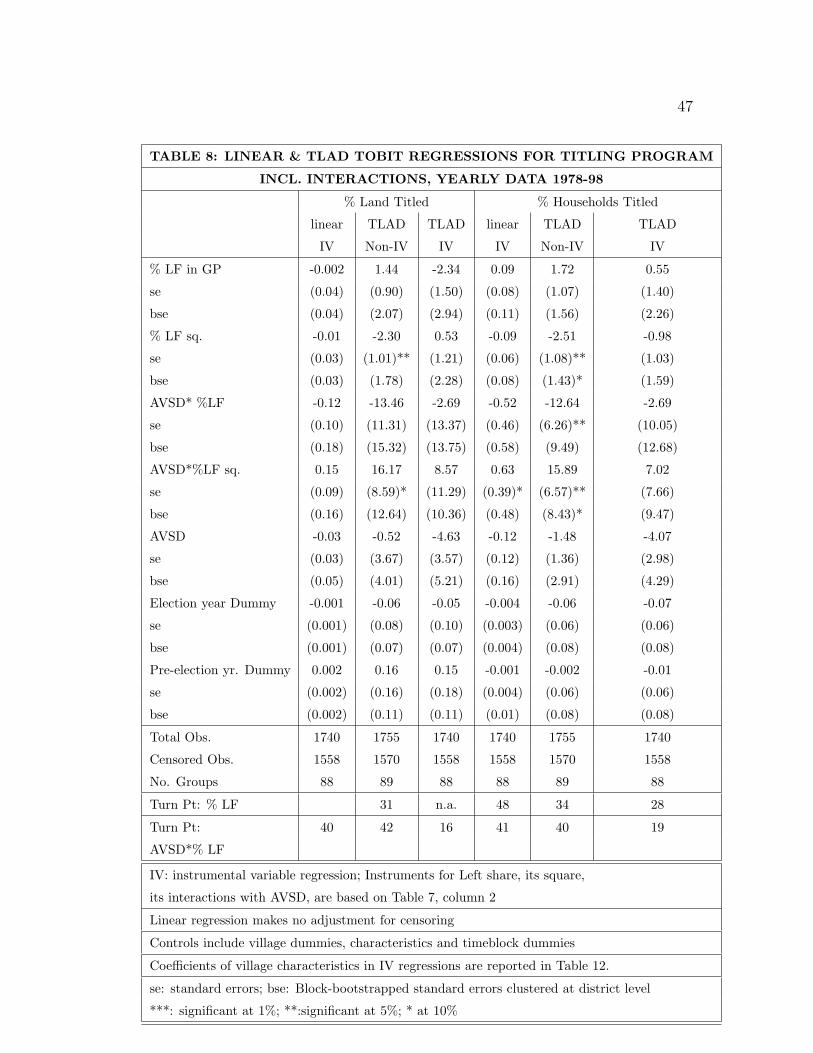
47

TABLE 8: LINEAR & TLAD TOBIT REGRESSIONS FOR TITLING PROGRAM

INCL. INTERACTIONS, YEARLY DATA 1978-98

% Land Titled % Households Titled

linear TLAD TLAD linear TLAD TLAD

IV Non-IV IV IV Non-IV IV

% LF in GP -0.002 1.44 -2.34 0.09 1.72 0.55

se (0.04) (0.90) (1.50) (0.08) (1.07) (1.40)

bse (0.04) (2.07) (2.94) (0.11) (1.56) (2.26)

% LF sq. -0.01 -2.30 0.53 -0.09 -2.51 -0.98

se (0.03) (1.01)** (1.21) (0.06) (1.08)** (1.03)

bse (0.03) (1.78) (2.28) (0.08) (1.43)* (1.59)

AVSD* %LF -0.12 -13.46 -2.69 -0.52 -12.64 -2.69

se (0.10) (11.31) (13.37) (0.46) (6.26)** (10.05)

bse (0.18) (15.32) (13.75) (0.58) (9.49) (12.68)

AVSD*%LF sq. 0.15 16.17 8.57 0.63 15.89 7.02

se (0.09) (8.59)* (11.29) (0.39)* (6.57)** (7.66)

bse (0.16) (12.64) (10.36) (0.48) (8.43)* (9.47)

AVSD -0.03 -0.52 -4.63 -0.12 -1.48 -4.07

se (0.03) (3.67) (3.57) (0.12) (1.36) (2.98)

bse (0.05) (4.01) (5.21) (0.16) (2.91) (4.29)

Election year Dummy -0.001 -0.06 -0.05 -0.004 -0.06 -0.07

se (0.001) (0.08) (0.10) (0.003) (0.06) (0.06)

bse (0.001) (0.07) (0.07) (0.004) (0.08) (0.08)

Pre-election yr. Dummy 0.002 0.16 0.15 -0.001 -0.002 -0.01

se (0.002) (0.16) (0.18) (0.004) (0.06) (0.06)

bse (0.002) (0.11) (0.11) (0.01) (0.08) (0.08)

Total Obs. 1740 1755 1740 1740 1755 1740

Censored Obs. 1558 1570 1558 1558 1570 1558

No. Groups 88 89 88 88 89 88

Turn Pt: % LF 31 n.a. 48 34 28

Turn Pt: 40 42 16 41 40 19

AVSD*% LF

IV: instrumental variable regression; Instruments for Left share, its square,

its interactions with AVSD, are based on Table 7, column 2

Linear regression makes no adjustment for censoring

Controls include village dummies, characteristics and timeblock dummies

Coefficients of village characteristics in IV regressions are reported in Table 12.

se: standard errors; bse: Block-bootstrapped standard errors clustered at district level

***: significant at 1%; **:significant at 5%; * at 10%

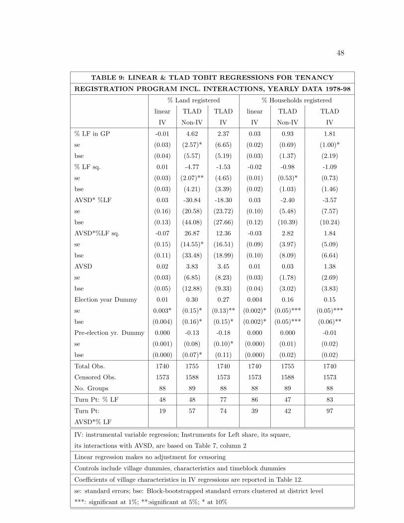
48

TABLE 9: LINEAR & TLAD TOBIT REGRESSIONS FOR TENANCY

REGISTRATION PROGRAM INCL. INTERACTIONS, YEARLY DATA 1978-98

% Land registered % Households registered

linear TLAD TLAD linear TLAD TLAD

IV Non-IV IV IV Non-IV IV

% LF in GP -0.01 4.62 2.37 0.03 0.93 1.81

se (0.03) (2.57)* (6.65) (0.02) (0.69) (1.00)*

bse (0.04) (5.57) (5.19) (0.03) (1.37) (2.19)

% LF sq. 0.01 -4.77 -1.53 -0.02 -0.98 -1.09

se (0.03) (2.07)** (4.65) (0.01) (0.53)* (0.73)

bse (0.03) (4.21) (3.39) (0.02) (1.03) (1.46)

AVSD* %LF 0.03 -30.84 -18.30 0.03 -2.40 -3.57

se (0.16) (20.58) (23.72) (0.10) (5.48) (7.57)

bse (0.13) (44.08) (27.66) (0.12) (10.39) (10.24)

AVSD*%LF sq. -0.07 26.87 12.36 -0.03 2.82 1.84

se (0.15) (14.55)* (16.51) (0.09) (3.97) (5.09)

bse (0.11) (33.48) (18.99) (0.10) (8.09) (6.64)

AVSD 0.02 3.83 3.45 0.01 0.03 1.38

se (0.03) (6.85) (8.23) (0.03) (1.78) (2.69)

bse (0.05) (12.88) (9.33) (0.04) (3.02) (3.83)

Election year Dummy 0.01 0.30 0.27 0.004 0.16 0.15

se 0.003* (0.15)* (0.13)** (0.002)* (0.05)*** (0.05)***

bse (0.004) (0.16)* (0.15)* (0.002)* (0.05)*** (0.06)**

Pre-election yr. Dummy 0.000 -0.13 -0.18 0.000 0.000 -0.01

se (0.001) (0.08) (0.10)* (0.000) (0.01) (0.02)

bse (0.000) (0.07)* (0.11) (0.000) (0.02) (0.02)

Total Obs. 1740 1755 1740 1740 1755 1740

Censored Obs. 1573 1588 1573 1573 1588 1573

No. Groups 88 89 88 88 89 88

Turn Pt: % LF 48 48 77 86 47 83

Turn Pt: 19 57 74 39 42 97

AVSD*% LF

IV: instrumental variable regression; Instruments for Left share, its square,

its interactions with AVSD, are based on Table 7, column 2

Linear regression makes no adjustment for censoring

Controls include village dummies, characteristics and timeblock dummies

Coefficients of village characteristics in IV regressions are reported in Table 12.

se: standard errors; bse: Block-bootstrapped standard errors clustered at district level

***: significant at 1%; **:significant at 5%; * at 10%

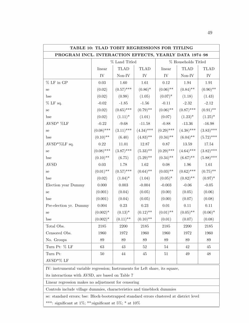
49

TABLE 10: TLAD TOBIT REGRESSIONS FOR TITLING

PROGRAM INCL. INTERACTION EFFECTS, YEARLY DATA 1974–98

% Land Titled % Households Titled

linear TLAD TLAD linear TLAD TLAD

IV Non-IV IV IV Non-IV IV

% LF in GP 0.03 1.60 1.61 0.12 1.94 1.91

se (0.02) (0.57)*** (0.86)* (0.06)** (0.84)** (0.90)**

bse (0.02) (0.98) (1.05) (0.07)* (1.18) (1.43)

% LF sq. -0.02 -1.85 -1.56 -0.11 -2.32 -2.12

se (0.02) (0.65)*** (0.79)** (0.06)** (0.87)*** (0.91)**

bse (0.02) (1.11)* (1.01) (0.07) (1.23)* (1.25)*

AVSD* %LF -0.22 -9.68 -11.58 -0.88 -13.36 -16.98

se (0.08)*** (3.11)*** (4.34)*** (0.29)*** (4.38)*** (3.83)***

bse (0.10)** (6.40) (4.83)** (0.34)** (6.04)** (5.72)***

AVSD*%LF sq. 0.22 11.01 12.87 0.87 13.59 17.54

se (0.08)*** (3.87)*** (5.33)** (0.29)*** (4.64)*** (3.82)***

bse (0.10)** (6.75) (5.29)** (0.34)** (6.67)** (5.88)***

AVSD 0.03 1.78 1.62 0.08 1.96 1.61

se (0.01)** (0.57)*** (0.64)** (0.03)** (0.62)*** (0.75)**

bse (0.02) (1.04)* (1.04) (0.05)* (0.82)** (0.97)*

Election year Dummy 0.000 0.003 -0.004 -0.003 -0.06 -0.05

se (0.001) (0.04) (0.05) (0.00) (0.05) (0.06)

bse (0.001) (0.04) (0.05) (0.00) (0.07) (0.08)

Pre-election yr. Dummy 0.004 0.23 0.23 0.01 0.11 0.11

se (0.002)* (0.13)* (0.12)** (0.01)** (0.05)** (0.06)*

bse (0.002)* (0.11)** (0.10)** (0.01) (0.07) (0.08)

Total Obs. 2185 2200 2185 2185 2200 2185

Censored Obs. 1960 1972 1960 1960 1972 1960

No. Groups 89 89 89 89 89 89

Turn Pt: % LF 63 43 52 54 42 45

Turn Pt: 50 44 45 51 49 48

AVSD*% LF

IV: instrumental variable regression; Instruments for Left share, its square,

its interactions with AVSD, are based on Table 7

Linear regression makes no adjustment for censoring

Controls include village dummies, characteristics and timeblock dummies

se: standard errors; bse: Block-bootstrapped standard errors clustered at district level

***: significant at 1%; **:significant at 5%; * at 10%

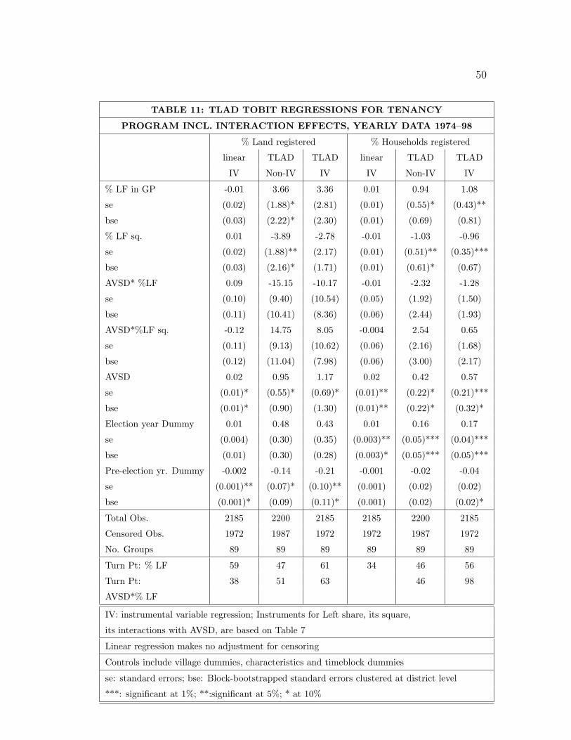
50

TABLE 11: TLAD TOBIT REGRESSIONS FOR TENANCY

PROGRAM INCL. INTERACTION EFFECTS, YEARLY DATA 1974–98

% Land registered % Households registered

linear TLAD TLAD linear TLAD TLAD

IV Non-IV IV IV Non-IV IV

% LF in GP -0.01 3.66 3.36 0.01 0.94 1.08

se (0.02) (1.88)* (2.81) (0.01) (0.55)* (0.43)**

bse (0.03) (2.22)* (2.30) (0.01) (0.69) (0.81)

% LF sq. 0.01 -3.89 -2.78 -0.01 -1.03 -0.96

se (0.02) (1.88)** (2.17) (0.01) (0.51)** (0.35)***

bse (0.03) (2.16)* (1.71) (0.01) (0.61)* (0.67)

AVSD* %LF 0.09 -15.15 -10.17 -0.01 -2.32 -1.28

se (0.10) (9.40) (10.54) (0.05) (1.92) (1.50)

bse (0.11) (10.41) (8.36) (0.06) (2.44) (1.93)

AVSD*%LF sq. -0.12 14.75 8.05 -0.004 2.54 0.65

se (0.11) (9.13) (10.62) (0.06) (2.16) (1.68)

bse (0.12) (11.04) (7.98) (0.06) (3.00) (2.17)

AVSD 0.02 0.95 1.17 0.02 0.42 0.57

se (0.01)* (0.55)* (0.69)* (0.01)** (0.22)* (0.21)***

bse (0.01)* (0.90) (1.30) (0.01)** (0.22)* (0.32)*

Election year Dummy 0.01 0.48 0.43 0.01 0.16 0.17

se (0.004) (0.30) (0.35) (0.003)** (0.05)*** (0.04)***

bse (0.01) (0.30) (0.28) (0.003)* (0.05)*** (0.05)***

Pre-election yr. Dummy -0.002 -0.14 -0.21 -0.001 -0.02 -0.04

se (0.001)** (0.07)* (0.10)** (0.001) (0.02) (0.02)

bse (0.001)* (0.09) (0.11)* (0.001) (0.02) (0.02)*

Total Obs. 2185 2200 2185 2185 2200 2185

Censored Obs. 1972 1987 1972 1972 1987 1972

No. Groups 89 89 89 89 89 89

Turn Pt: % LF 59 47 61 34 46 56

Turn Pt: 38 51 63 46 98

AVSD*% LF

IV: instrumental variable regression; Instruments for Left share, its square,

its interactions with AVSD, are based on Table 7

Linear regression makes no adjustment for censoring

Controls include village dummies, characteristics and timeblock dummies

se: standard errors; bse: Block-bootstrapped standard errors clustered at district level

***: significant at 1%; **:significant at 5%; * at 10%

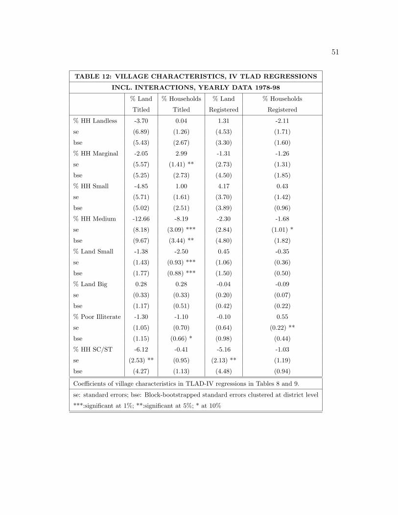
51

TABLE 12: VILLAGE CHARACTERISTICS, IV TLAD REGRESSIONS

INCL. INTERACTIONS, YEARLY DATA 1978-98

% Land % Households % Land % Households

Titled Titled Registered Registered

% HH Landless -3.70 0.04 1.31 -2.11

se (6.89) (1.26) (4.53) (1.71)

bse (5.43) (2.67) (3.30) (1.60)

% HH Marginal -2.05 2.99 -1.31 -1.26

se (5.57) (1.41) ** (2.73) (1.31)

bse (5.25) (2.73) (4.50) (1.85)

% HH Small -4.85 1.00 4.17 0.43

se (5.71) (1.61) (3.70) (1.42)

bse (5.02) (2.51) (3.89) (0.96)

% HH Medium -12.66 -8.19 -2.30 -1.68

se (8.18) (3.09) *** (2.84) (1.01) *

bse (9.67) (3.44) ** (4.80) (1.82)

% Land Small -1.38 -2.50 0.45 -0.35

se (1.43) (0.93) *** (1.06) (0.36)

bse (1.77) (0.88) *** (1.50) (0.50)

% Land Big 0.28 0.28 -0.04 -0.09

se (0.33) (0.33) (0.20) (0.07)

bse (1.17) (0.51) (0.42) (0.22)

% Poor Illiterate -1.30 -1.10 -0.10 0.55

se (1.05) (0.70) (0.64) (0.22) **

bse (1.15) (0.66) * (0.98) (0.44)

% HH SC/ST -6.12 -0.41 -5.16 -1.03

se (2.53) ** (0.95) (2.13) ** (1.19)

bse (4.27) (1.13) (4.48) (0.94)

Coefficients of village characteristics in TLAD-IV regressions in Tables 8 and 9.

se: standard errors; bse: Block-bootstrapped standard errors clustered at district level

***:significant at 1%; **:significant at 5%; * at 10%

LEFT’S WINPROBABILITY

LANDREFORM

RIGHT PARTY’S POLICY

LEFT PARTY’S POLICY

Figure 1: Case 1: Political Moral Hazard Effect Dominates

LEFT’S POLICY

RIGHT’S POLICY

LEFT’S WINPROBABILITY

LANDREFORM

Figure 2: Case 2: Ideology Dominates

48