EDUCATION AND EXAMINATION COMMITTEE

OF THE

SOCIETY OF ACTUARIES

FINANCIAL MATHEMATICS STUDY NOTE

DETERMINANTS OF INTEREST RATES

by

Michael A. Bean, FSA, CERA FCIA, FCAS, PhD

Copyright 2017 by the Society of Actuaries The Education and Examination Committee provides study notes to persons preparing for the examinations of the Society of Actuaries. They are intended to acquaint candidates with some of the theoretical and practical considerations involved in the various subjects. While varying opinions are presented where appropriate, limits on the length of the material and other considerations sometimes prevent the inclusion of all possible opinions. These study notes do not, however, represent any official opinion, interpretations or endorsement of the Society of Actuaries or its Education and Examination Committee. The Society is grateful to the authors for their contributions in preparing the study notes.

FM-26-17

1

Determinants of Interest Rates Michael A. Bean, FSA, CERA, FCIA, FCAS, PhD

May, 2017

Contents 1 Introduction ............................................................................................................................. 3

2 Background ............................................................................................................................. 3

2.1 What is interest? ............................................................................................................... 3

2.2 Quotation bases for interest rates ..................................................................................... 6

2.2.1 Rates on U.S. Treasury Bills ..................................................................................... 6

2.2.2 Rates on Government of Canada Treasury Bills ....................................................... 7

2.2.3 Effective and Continuously Compounded Rates ...................................................... 7

3 Understanding the Components of the Interest Rate .............................................................. 8

3.1 Interest rates in a world of no inflation or default risk ..................................................... 9

3.1.1 Interest Rates by Term .............................................................................................. 9

3.1.2 Yield Curves ........................................................................................................... 11

3.2 Interest rates in a world of no inflation but in which defaults can occur ....................... 12

3.2.1 Default with No Recovery ...................................................................................... 13

3.2.2 Default with Partial Recovery ................................................................................. 15

3.2.3 Compensation for Default Risk .............................................................................. 16

3.3 Interest rates in a world of known inflation ................................................................... 16

3.4 Interest rates in a world of uncertain inflation ............................................................... 19

3.4.1 Loans with Inflation Protection .............................................................................. 19

3.4.2 Loans without Inflation Protection ......................................................................... 21

3.4.3 Real and Nominal Interest Rates............................................................................. 21

3.4.4 Decomposition of the Interest Rate When Defaults are Possible ........................... 22

4 Retail Savings and Lending Interest Rates ........................................................................... 23

4.1 Banks as intermediaries between borrowers and savers ................................................ 23

4.2 Savings Interest rates ...................................................................................................... 24

4.3 Lending Interest rates ..................................................................................................... 25

5 Bonds Issued by Governments and Corporations ................................................................. 26

5.1 Zero-coupon bonds ......................................................................................................... 27

2

5.2 U.S. Treasury securities ................................................................................................. 28

5.3 State and local government bonds in the United States ................................................. 32

5.4 Government bonds in Canada ........................................................................................ 32

5.5 Corporate bonds ............................................................................................................. 34

6 The Role of Central Banks .................................................................................................... 37

6.1 Operation of the payment system ................................................................................... 37

6.2 Lender of last resort........................................................................................................ 38

6.3 The United States Federal Reserve Bank System .......................................................... 39

3

1 Introduction Interest rates arise in some form in virtually every calculation in actuarial science and finance. This study note is intended to provide an overview of what interest rates represent, how they arise in practice, and the factors that determine their value.

We begin by considering what interest represents from an economic perspective and how interest rates are expressed in practice. We next consider the effect that defaults, inflation, and other factors can have on the value of interest rates, and show how an interest rate can be decomposed into component parts with each component viewed as compensation for a particular risk. We then consider some situations where interest rates arise in practice, including retail savings and lending products and bonds issued by governments or corporations; key takeaways from this discussion are that interest rates can differ greatly from one product or borrower to another and can fluctuate by material amounts over time. We end with a discussion of the role of central banks and how their actions can influence the general level of interest rates.

2 Background

2.1 WHAT IS INTEREST? From an economic perspective, interest can be viewed as either the compensation received for deferring consumption, e.g., putting money in a savings account rather than spending it, or the cost of consuming when resources are not available, e.g., using a credit card to make a purchase rather than first saving the money. At any given time, a person with money has two choices. One is to spend the money today and the second is to save it for the future. Likewise, a person without money has two choices. One is to borrow money from someone to buy something and the second is to decide to postpone the purchase. The decision whether to spend, save, borrow, or refrain from spending can be a complex one. Some people require a greater incentive to save, i.e., the reward for deferring consumption needs to be greater, while others require a greater incentive to borrow, i.e., the cost of borrowing needs to be lower.

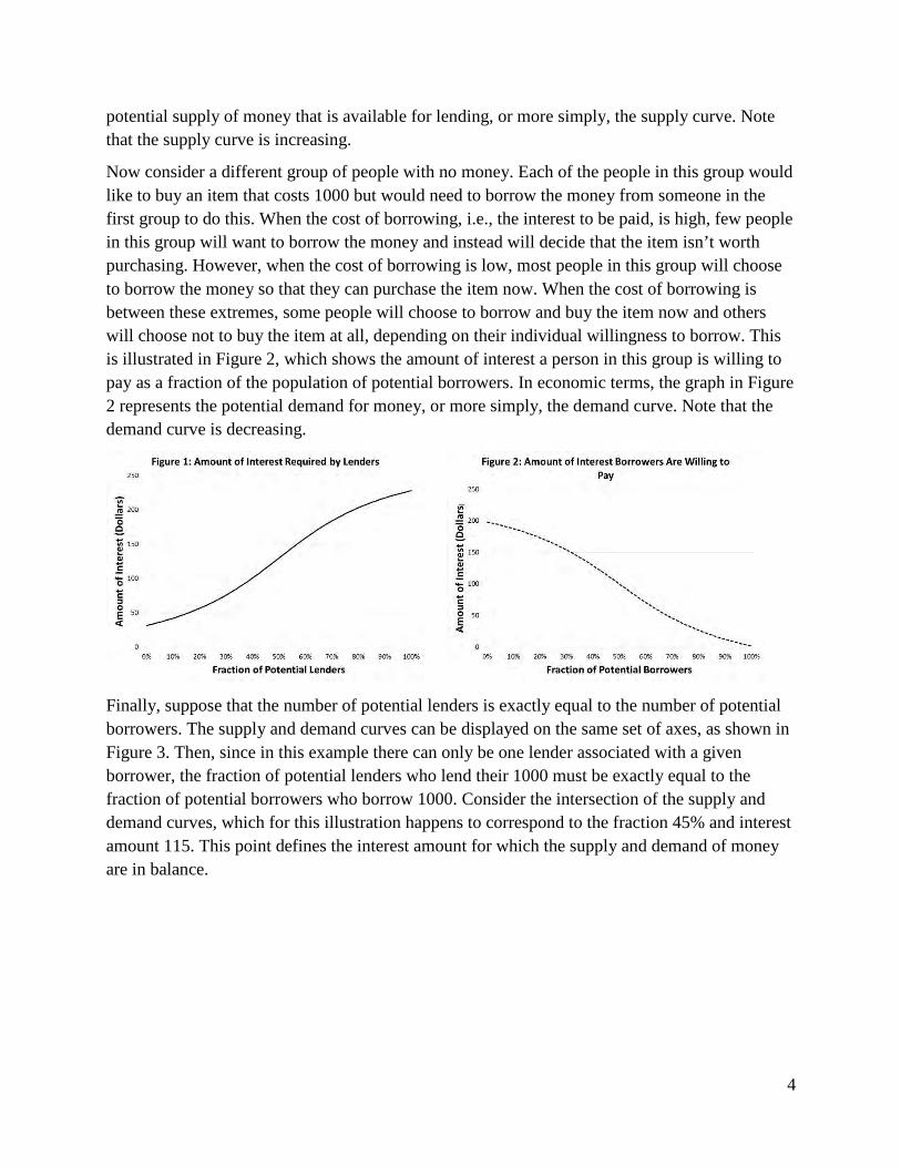
Consider a group of people, each with 10001 that can either be spent today or lent to someone who will repay the loan with interest in two years. When the compensation for lending, i.e., the interest received, is low, few people in the group will want to lend their 1000 and instead will choose to spend it on themselves. However, when the compensation for lending is high, most people in the group will choose to lend their 1000 and defer their own spending. When the compensation for lending is between these extremes, some people will choose to spend and others will choose to lend, depending on their individual preferences to save versus spend. This is illustrated graphically in Figure 1, which shows the amount of interest required as a fraction of the population of potential lenders. In economic terms, the graph in Figure 1 represents the

1 The currency being used (dollars, euros, etc.) is not relevant to the discussions in this note. Hence, no currency symbols will be attached to monetary amounts.

4

potential supply of money that is available for lending, or more simply, the supply curve. Note that the supply curve is increasing.

Now consider a different group of people with no money. Each of the people in this group would like to buy an item that costs 1000 but would need to borrow the money from someone in the first group to do this. When the cost of borrowing, i.e., the interest to be paid, is high, few people in this group will want to borrow the money and instead will decide that the item isn’t worth purchasing. However, when the cost of borrowing is low, most people in this group will choose to borrow the money so that they can purchase the item now. When the cost of borrowing is between these extremes, some people will choose to borrow and buy the item now and others will choose not to buy the item at all, depending on their individual willingness to borrow. This is illustrated in Figure 2, which shows the amount of interest a person in this group is willing to pay as a fraction of the population of potential borrowers. In economic terms, the graph in Figure 2 represents the potential demand for money, or more simply, the demand curve. Note that the demand curve is decreasing.

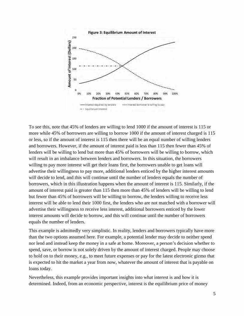
Finally, suppose that the number of potential lenders is exactly equal to the number of potential borrowers. The supply and demand curves can be displayed on the same set of axes, as shown in Figure 3. Then, since in this example there can only be one lender associated with a given borrower, the fraction of potential lenders who lend their 1000 must be exactly equal to the fraction of potential borrowers who borrow 1000. Consider the intersection of the supply and demand curves, which for this illustration happens to correspond to the fraction 45% and interest amount 115. This point defines the interest amount for which the supply and demand of money are in balance.

5

To see this, note that 45% of lenders are willing to lend 1000 if the amount of interest is 115 or more while 45% of borrowers are willing to borrow 1000 if the amount of interest charged is 115 or less, so if the amount of interest is 115 then there will be an equal number of willing lenders and borrowers. However, if the amount of interest paid is less than 115 then fewer than 45% of lenders will be willing to lend but more than 45% of borrowers will be willing to borrow, which will result in an imbalance between lenders and borrowers. In this situation, the borrowers willing to pay more interest will get their loans first, the borrowers unable to get loans will advertise their willingness to pay more, additional lenders enticed by the higher interest amounts will decide to lend, and this will continue until the number of lenders equals the number of borrowers, which in this illustration happens when the amount of interest is 115. Similarly, if the amount of interest paid is greater than 115 then more than 45% of lenders will be willing to lend but fewer than 45% of borrowers will be willing to borrow, the lenders willing to receive less interest will be able to lend their 1000 first, the lenders who are not matched with a borrower will advertise their willingness to receive less interest, additional borrowers enticed by the lower interest amounts will decide to borrow, and this will continue until the number of borrowers equals the number of lenders.

This example is admittedly very simplistic. In reality, lenders and borrowers typically have more than the two options assumed here. For example, a potential lender may decide to neither spend nor lend and instead keep the money in a safe at home. Moreover, a person’s decision whether to spend, save, or borrow is not solely driven by the amount of interest charged. People may choose to hold on to their money, e.g., to meet future expenses or pay for the latest electronic gizmo that is expected to hit the market a year from now, whatever the amount of interest that is payable on loans today.

Nevertheless, this example provides important insights into what interest is and how it is determined. Indeed, from an economic perspective, interest is the equilibrium price of money

6

and is defined by the intersection of the supply and demand curves for money. Moreover, this equilibrium price is not static. When there are shifts in the supply or demand curves for money as may occur, for example, when a new product is introduced or expected to be introduced to the market, the equilibrium amount of interest and number of loans will also change.

2.2 QUOTATION BASES FOR INTEREST RATES There are many different ways in which interest rates can be quoted. Some quotation conventions are primarily historical, dating from a time when interest calculations had to be done mentally or using pencil and paper; others may be the result of legal statutes designed to protect consumers against unscrupulous advertising practices. Because there are many different ways in which interest rates can be quoted, it is important to be aware of the particular quotation basis that is used in a given application so that the inferences one makes are meaningful.

Here we highlight a few important quotation bases that frequently arise in practice and show that for a given loan or investment, the interest rates determined using different quotation bases can be materially different.

2.2.1 RATES ON U.S. TREASURY BILLS As an example, consider a government Treasury bill, which is a short-term debt security issued by a government for the purpose of meeting short-term cash flow obligations. It is essentially a loan to the government. By convention, government Treasury bills have a term less than one year, typically three months or six months, at issue, and a maturity value that is a fixed, round number such as 10,000, 100,000, 1 million, etc.

A U.S. Treasury bill, commonly referred to as a U.S. T-bill, is quoted using the following formula:

360 Dollar amount of interestQuoted rateDays to maturity Maturity value of the Treasury bill

= ×

where “Days to maturity” is the remaining number of days until maturity. For example, a 90-day T-bill with maturity value 10,000 and price 9800 would have a quoted rate at issue of 8% (= 360/90 × 200/10,000).

The quoted rate on a U.S. T-bill can be quite different from the interest rate defined by the usual compound interest formula 0 (1 )t

tP P i= ⋅ + . Substituting 0 9800P = , 10,000tP = , and t = 90/365 into the compound interest formula and solving for 𝑖𝑖 we find that i = 8.54% (rounded to two decimal places). The interest rate defined by the compound interest formula is a more accurate representation of the rate of growth than the quoted rate, but it can be difficult to calculate quickly without the assistance of a calculator or computer. By contrast, the quoted rate is very simple to calculate, particularly when the maturity value is a multiple of 10,000; in fact, the calculation can be done mentally, which was undoubtedly an attractive feature in the 1930s, 1940s and 1950s.

7

2.2.2 RATES ON GOVERNMENT OF CANADA TREASURY BILLS Not all government Treasury bills follow the same quotation convention as U.S. T-bills. For example, Treasury bills issued by the Government of Canada are quoted using the following formula:

365 Dollar amount of interestQuoted rate .Days to maturity Current price of Treasury bill

= ×

In particular, the quoted rate is calculated with respect to the current price of the T-bill rather than its maturity value and the number of days in a year is assumed to be 365 rather than 360. With this convention, a Government of Canada T-bill with maturity value 10,000, current price 9800 and 90 days to maturity would have a quoted rate of approximately 8.28% (=365/90 × 200/9800). Note that this is materially different from the 8% rate that would be quoted using the U.S. T-bill convention or the 8.54% rate that would be determined using the compound interest formula.

This example nicely illustrates why it is important to be aware of the quotation basis used in a given application, particularly when the application involves working with historical data. Indeed, we see that if one blindly compares the rates on U.S. and Government of Canada T-bills with identical terms without adjusting for differences in quotation basis, one might conclude that Government of Canada T-bills pay more interest when in fact the interest paid on both T-bills is the same.

2.2.3 EFFECTIVE AND CONTINUOUSLY COMPOUNDED RATES To minimize the possibility of error due to the mixing of quotation bases, it is good practice to convert all the interest rates in a given problem to a common basis. For this purpose, two quotation bases are particularly noteworthy. The first defines rates by the compound interest formula mentioned earlier:

0 (1 ) .ttP P i= ⋅ +

The interest rate 𝑖𝑖 defined by this formula is referred to as the effective interest rate; when 𝑡𝑡 is measured in years, it is the effective per annum interest rate. The second defines rates by the alternative compound interest formula:

0 .rttP P e= ⋅

The interest rate 𝑟𝑟 defined by this latter formula is referred to as the continuously compounded rate or the force of interest; when 𝑡𝑡 is measured in years, it is the continuously compounded per annum interest rate.

When comparing quoted interest rates it is important to know the definition used. For example, in advertisements for car loans, phrases such as “annual percentage yield (APY)” or “annual percentage rate (APR)” often accompany a quoted rate. The APR is typically a nominal rate,

8

while the APY is typically an effective per annum rate. U.S. government regulations require that the APR be disclosed to borrowers; however, reading the fine print is always a good idea.

Continuously compounded rates are easier to work with from a mathematical perspective and for this reason are most often used in economic and actuarial modeling applications. Continuously compounded rates are additive, whereas effective rates are not. For example, consider an investment that earns a different rate each year. If the rates are quoted in continuously compounded form, then the accumulation after 𝑛𝑛 years is

1 21 20 0 ,n nr r r rr rP e e e P e + + +⋅ ⋅ = ⋅

where 1 2, , , nr r r are the continuously compounded rates for the respective years. If 𝑟𝑟 is the

equivalent continuously compounded rate for the entire 𝑛𝑛-year period then 1 20 0

nr r rrnP e P e + + +⋅ = ⋅ ,

which implies that 1 2( ) /nr r r r n= + + + . Similarly, if the rates are quoted in effective form then the equivalent per annum rate for the n year period is easily seen to be

1/1 2[(1 ) (1 ) (1 )] 1n

ni i i i= + ⋅ + + − . Clearly, the mathematics of compounding is much simpler when rates are quoted in continuous form.

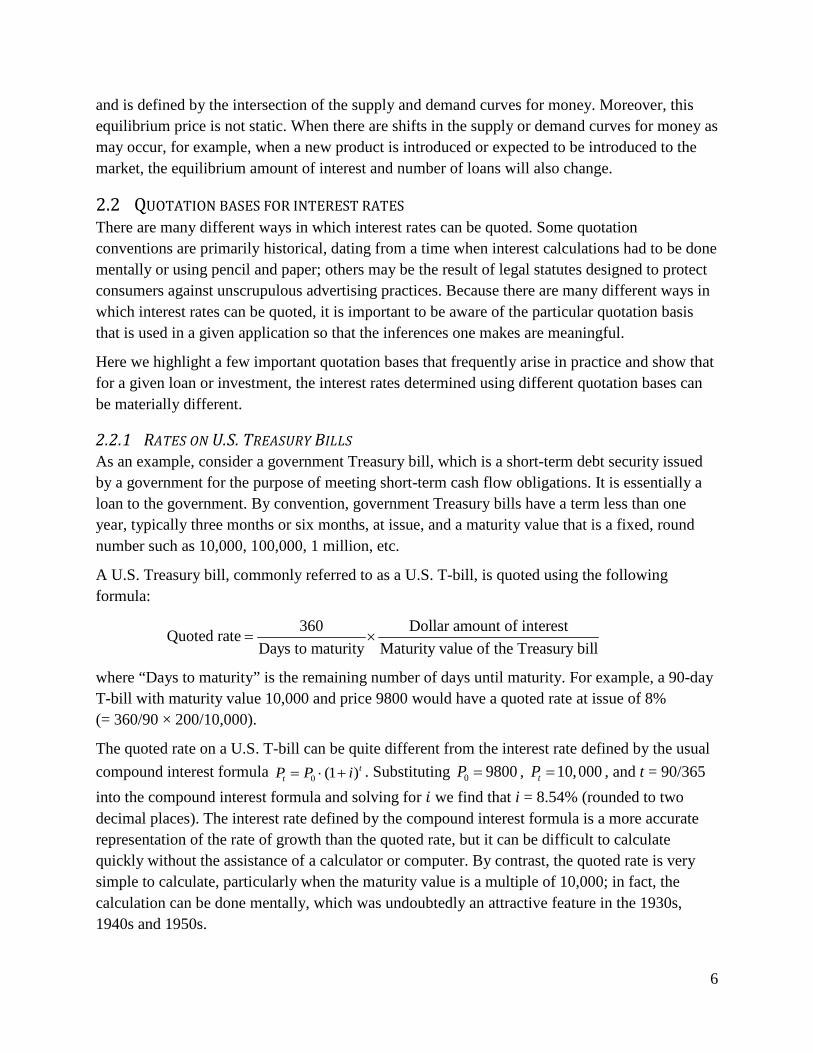
Returning to the example of the 90-day T-bill with maturity value 10,000 and current price 9800, we see from the formula for compound interest in continuous terms that the interest rate on this T-bill expressed in continuous per annum form is approximately 8.19%. This rate is lower than the rate in effective per annum form but higher than the rate using the standard quotation convention for U.S. Treasury bills. These observations are summarized in Table 1.

Table 1: Quoted Rates for a 90-day T-bill with Price 9800 per 10,000 of Maturity Value

U.S. T-bill convention

Government of Canada T-bill

convention

Continuously compounded per

annum Effective per

annum 8.00% 8.28% 8.19% 8.54%

3 Understanding the Components of the Interest Rate In the previous chapter, we saw that from an economic perspective interest is the compensation received for deferring consumption, or equivalently, the cost of consuming before acquiring the necessary assets, and interest rates can be viewed as the equilibrium price of money. Hence, an important determinant of interest rates is the supply and demand of money. In this chapter, we consider additional determinants of interest rates including the length of time money is lent, the extent to which there is a risk that lent money is not fully repaid, and the extent to which money loses its purchasing power over time. We will see that when interest rates are expressed in continuous form, they can be decomposed into a sum with one term representing compensation for deferring consumption, another compensation for lost purchasing power, another compensation for the risk of default, and so on.

9

3.1 INTEREST RATES IN A WORLD OF NO INFLATION OR DEFAULT RISK Let’s begin by considering interest rates in a world in which the prices of goods and services do not change over time and all loans are fully repaid on time according to the terms originally agreed upon, i.e., there is no monetary inflation and no risk of default. Such a world does not exist, of course; prices of goods and services do change, generally increasing over time, and people do not always repay loans in full or on time. However, for the purposes of discovering additional determinants of interest rates, this is a useful starting point.

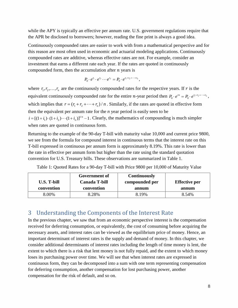
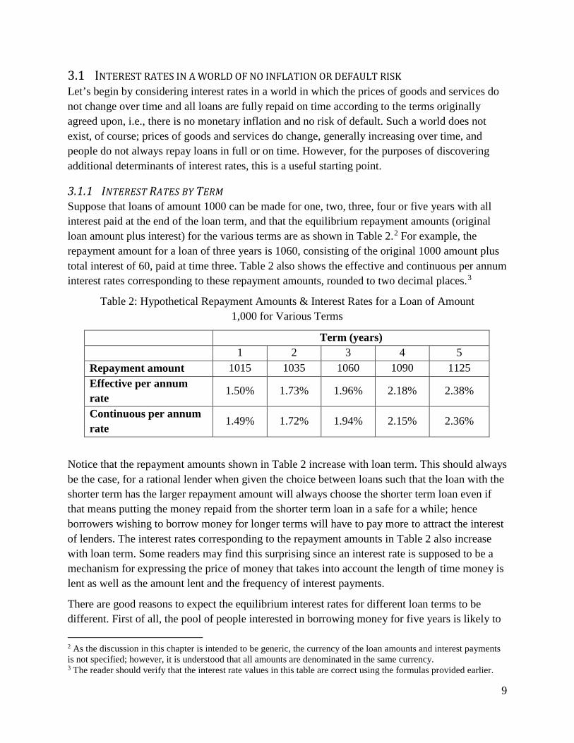
3.1.1 INTEREST RATES BY TERM Suppose that loans of amount 1000 can be made for one, two, three, four or five years with all interest paid at the end of the loan term, and that the equilibrium repayment amounts (original loan amount plus interest) for the various terms are as shown in Table 2.2 For example, the repayment amount for a loan of three years is 1060, consisting of the original 1000 amount plus total interest of 60, paid at time three. Table 2 also shows the effective and continuous per annum interest rates corresponding to these repayment amounts, rounded to two decimal places.3

Table 2: Hypothetical Repayment Amounts & Interest Rates for a Loan of Amount 1,000 for Various Terms

Term (years) 1 2 3 4 5 Repayment amount 1015 1035 1060 1090 1125 Effective per annum rate

1.50% 1.73% 1.96% 2.18% 2.38%

Continuous per annum rate

1.49% 1.72% 1.94% 2.15% 2.36%

Notice that the repayment amounts shown in Table 2 increase with loan term. This should always be the case, for a rational lender when given the choice between loans such that the loan with the shorter term has the larger repayment amount will always choose the shorter term loan even if that means putting the money repaid from the shorter term loan in a safe for a while; hence borrowers wishing to borrow money for longer terms will have to pay more to attract the interest of lenders. The interest rates corresponding to the repayment amounts in Table 2 also increase with loan term. Some readers may find this surprising since an interest rate is supposed to be a mechanism for expressing the price of money that takes into account the length of time money is lent as well as the amount lent and the frequency of interest payments.

There are good reasons to expect the equilibrium interest rates for different loan terms to be different. First of all, the pool of people interested in borrowing money for five years is likely to 2 As the discussion in this chapter is intended to be generic, the currency of the loan amounts and interest payments is not specified; however, it is understood that all amounts are denominated in the same currency. 3 The reader should verify that the interest rate values in this table are correct using the formulas provided earlier.

10

be different from the pool of people interested in borrowing money for just one year. A person who borrows money for just one year usually does so to cover a short-term cash flow shortfall and expects to be able to earn enough money during the year to repay the loan with interest by year’s end. However, a person who borrows money for five years generally needs the money for that length of time, e.g., to fund the start up of a new business venture or purchase some durable good, and expects it will take several years to earn enough money to repay the loan. Likewise, the pool of people interested in lending money for five years is likely to be different from the pool of people interested in lending money for just one year. People who lend money for five years or more are generally saving for some long-term goal such as retirement and don’t mind having their money tied up for an extended period of time whereas people who lend money for just one year are generally saving for some shorter term goal and want to be able to access their money within that shorter timeframe. Since the pools of borrowers and lenders are generally different for different loan terms, it follows that the supply and demand dynamics of money are also different, and hence the equilibrium interest rates will differ. This explanation for the difference in interest rates by term is called the market segmentation theory.

Secondly, even if the pool of lenders is not strictly differentiated by term and some lenders who might otherwise prefer one term could be persuaded to lend for another, there must be some incentive for them to do so. All things being equal, lenders tend to prefer to lend money for shorter terms because this gives them the flexibility to take advantage of alternative investment opportunities that may arise during the course of a longer term. Hence, to persuade lenders to lend money for the longer term, borrowers generally have to pay a higher rate of interest, not just higher compensation. This explanation is called the liquidity preference theory or the opportunity cost theory.

There are two additional theories that have been postulated to explain why interest rates differ by term. One is the expectations theory. According to this theory, the interest rate on a longer term loan provides information on the interest rates that shorter term loans are expected to have in the future; for example, if the interest rate on a three-year loan is currently greater than the interest rate on a one-year loan then two years from now, the rate on a one-year loan will be higher than it is now. The final one is the preferred habitat theory. Similar to the market segmentation theory, this theory asserts that differences in interest rates are attributable to differences in the pools of lenders and borrowers; however, lenders and borrowers are not rigidly segmented by term. Given sufficient incentive to do so, market participants are willing to move to a term that is different from their preferred one.

Although not a frequent occurrence, interest rates can decrease with term. There are several reasons this could happen. There could be a decrease in the pool of people interested in lending money for shorter terms because they need the money themselves, e.g., to buy the latest electronic gizmo or to pay bills during a period of unemployment. In this case, the supply curve for short-term money shifts upwards and to the left, and the equilibrium interest rate increases (see Figures 1 and 3 in the previous chapter). At the same time, there could be an increase in the

11

pool of people interested in borrowing money for shorter terms, e.g., to pay expenses during a period of reduced cash flow; in this case, the demand curve for short term money shift upwards and to the right, and the equilibrium interest rate increases once again (see Figures 2 and 3 in the previous chapter). There could also be a decrease in the pool of people interested in borrowing money for longer terms. This could happen, for example, if the economy is weaker than normal, the rate of return on long-term investments is not sufficiently high to justify the cost of borrowing, and/or the risk of entering into a long-term venture is higher than normal. In this case, the demand curve for long term money shifts downwards and to the left, and the equilibrium long term interest rate declines.

Interest rates can also increase and then decrease with term. In this case, the cost of medium-term money is greater than the cost of either short-term or long-term money. The reader is invited to contemplate situations where this could occur.

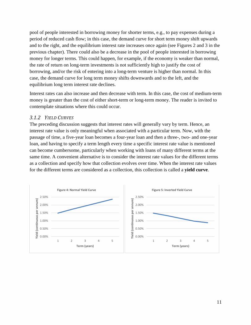
3.1.2 YIELD CURVES The preceding discussion suggests that interest rates will generally vary by term. Hence, an interest rate value is only meaningful when associated with a particular term. Now, with the passage of time, a five-year loan becomes a four-year loan and then a three-, two- and one-year loan, and having to specify a term length every time a specific interest rate value is mentioned can become cumbersome, particularly when working with loans of many different terms at the same time. A convenient alternative is to consider the interest rate values for the different terms as a collection and specify how that collection evolves over time. When the interest rate values for the different terms are considered as a collection, this collection is called a yield curve.

0.00%

0.50%

1.00%

1.50%

2.00%

2.50%

1 2 3 4 5

Yiel

d (c

ontin

uous

per

ann

um)

Term (years)

Figure 4: Normal Yield Curve

0.00%

0.50%

1.00%

1.50%

2.00%

2.50%

1 2 3 4 5

Yiel

d (c

ontin

uous

per

ann

um)

Term (years)

Figure 5: Inverted Yield Curve

12

The yield curve corresponding to Table 2 is shown in Figure 4. Note that the curve in this case slopes upwards. This is the expected shape because, as noted earlier, lenders tend to prefer to lend money for shorter terms and hence generally must be provided an incentive to lend for a longer term. Figure 5 shows a yield curve when interest rates decrease with term and Figure 6 shows one when interest rates increase and then decrease. Note that the yield curve in Figure 5 slopes downwards and the one in Figure 6 has the shape of a bow, sloping upwards and then downwards.

With these observations in mind, we can define the following terms. A yield curve is said to be normal or upward-sloping if the interest rate values increase with term; it is said to be inverted or downward-sloping if the interest rate values decrease with term; and it is said to be bowed if the interest rate values increase and then decrease with term, or decrease and then increase with term. A yield curve is said to be flat if the interest rate values are the same for all terms. Figure 7 provides an illustration of a flat yield curve.

Flat yield curves rarely arise in practice. However, many simple models of interest rates and interest rate movements nevertheless assume that yield curves are flat. For example, the concept of duration, which is widely used in the management of bond portfolios is based on this assumption. The traditional formulas for mortgage and annuity mathematics, are also based on this assumption. As long as the user is aware that it is an approximation, the assumption that yield curves are flat can help to simplify a problem and allow general insights to be gained. However, it is important to remember that this is an idealized assumption and that in general yield curves are not flat.

3.2 INTEREST RATES IN A WORLD OF NO INFLATION BUT IN WHICH DEFAULTS CAN OCCUR Now consider a world in which defaults can occur, i.e., there is a risk that some borrowers will not fully repay the amount lent on time and with interest at the agreed upon terms. For simplicity, continue to assume that the prices of goods and services do not change over time, i.e., there is no monetary inflation.

0.00%

0.50%

1.00%

1.50%

2.00%

2.50%

1 2 3 4 5

Yiel

d (c

ontin

uous

per

ann

um)

Term (years)

Figure 6: Bow-Shaped Yield Curve

0.00%

0.50%

1.00%

1.50%

2.00%

2.50%

1 2 3 4 5

Yiel

d (c

ontin

uous

per

ann

um)

Term (years)

Figure 7: Flat Yield Curve

13

3.2.1 DEFAULT WITH NO RECOVERY Suppose that there are two types of borrowers, those who always repay loans in full and on time and those for whom defaults though rare are possible. Suppose further that for borrowers who are certain to repay their loans in full and on time, the equilibrium repayment amounts and interest rates for a loan of 1000 are the same as given in Table 2 earlier, and for borrowers for whom defaults are possible, the number of defaults per 1000 borrowers are as given in Table 3. For example, for a loan with a term of three years, ten out of 1000 borrowers will pay nothing at the end of three years. What can be said about the repayment amount and interest rate for a loan of 1000 of a specified term to a borrower for whom default is possible?

Table 3: Assumed Number of Defaults Over Loan Term per 1000 Loans

Term (years) 1 2 3 4 5

Number of defaults 2 5 10 16 25

To answer this question, consider a group of 1000 borrowers each of whom seeks to borrow the amount 1000 for a term of three years and suppose that out of this group of 1000 borrowers it is known in advance that precisely ten will default, but not which ten. Let x be the contractual repayment amount at time three. Then, the total amount received by the lender at time three is (990 · x) + (10 · 0) = 990 · x.

Suppose that a lender has the amount one million to lend for three years and is considering providing a loan of 1000 to each of these 1000 borrowers but also has the option of lending the money to a group of 1000 borrowers, each of whom is certain to repay the loan amount on time with interest. From Table 2, we know that the equilibrium repayment amount for a three-year loan for which repayment is certain is 1060, so if the lender chooses to lend the one million amount to the 1,000 borrowers who are certain to repay, the lender is certain to receive the amount 1000 · 1060 = 1,060,000 at the end of three years. On the other hand, if the lender chooses to lend the one million amount to the 1000 borrowers for whom repayment is not certain, the lender will receive the amount 990 · x at the end of three years. Consequently, for the lender to be willing to provide loans to the 1000 borrowers for whom repayment is not certain, the following inequality must be true:

990 1,060,000,x⋅ ≥ i.e.,

1070.71.x ≥

Hence, when repayment is not certain, the repayment amount on a three-year loan of 1000 must be at least 1070.71 (rounded to two decimal places). This corresponds to an effective per annum interest rate of 2.30% and a continuous per annum rate of 2.28%.

14

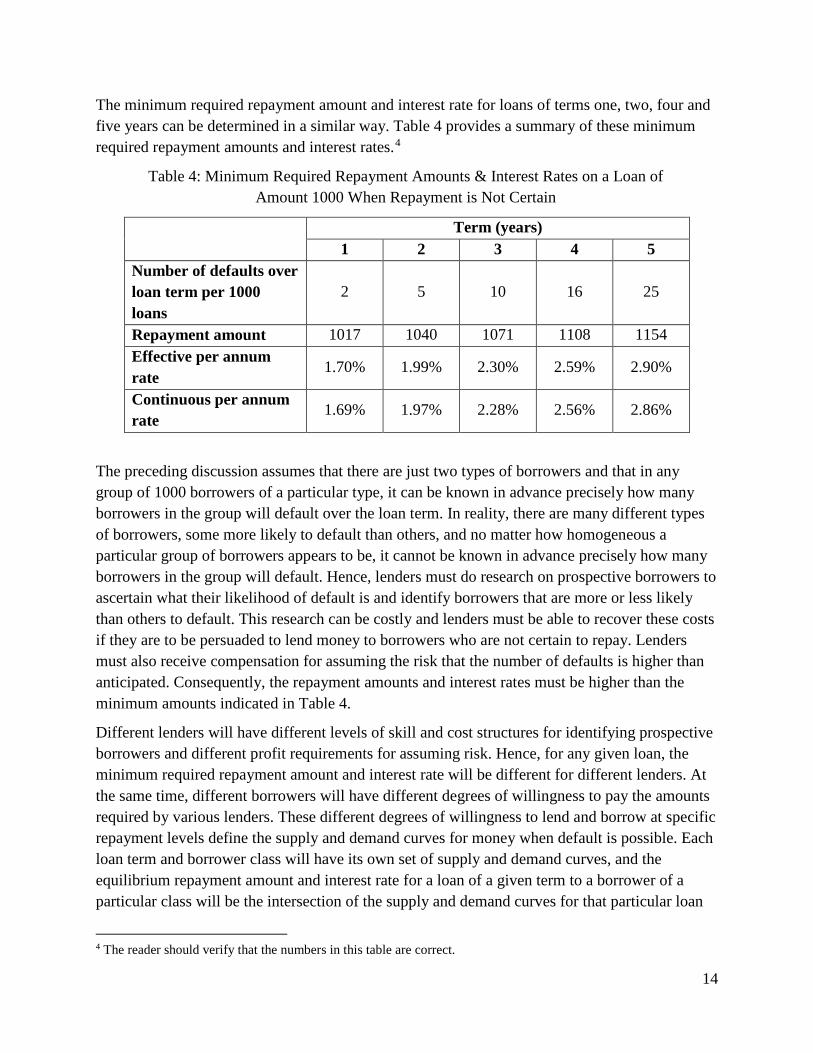
The minimum required repayment amount and interest rate for loans of terms one, two, four and five years can be determined in a similar way. Table 4 provides a summary of these minimum required repayment amounts and interest rates.4

Table 4: Minimum Required Repayment Amounts & Interest Rates on a Loan of Amount 1000 When Repayment is Not Certain

Term (years)

1 2 3 4 5 Number of defaults over loan term per 1000 loans

2 5 10 16 25

Repayment amount 1017 1040 1071 1108 1154 Effective per annum rate

1.70% 1.99% 2.30% 2.59% 2.90%

Continuous per annum rate

1.69% 1.97% 2.28% 2.56% 2.86%

The preceding discussion assumes that there are just two types of borrowers and that in any group of 1000 borrowers of a particular type, it can be known in advance precisely how many borrowers in the group will default over the loan term. In reality, there are many different types of borrowers, some more likely to default than others, and no matter how homogeneous a particular group of borrowers appears to be, it cannot be known in advance precisely how many borrowers in the group will default. Hence, lenders must do research on prospective borrowers to ascertain what their likelihood of default is and identify borrowers that are more or less likely than others to default. This research can be costly and lenders must be able to recover these costs if they are to be persuaded to lend money to borrowers who are not certain to repay. Lenders must also receive compensation for assuming the risk that the number of defaults is higher than anticipated. Consequently, the repayment amounts and interest rates must be higher than the minimum amounts indicated in Table 4.

Different lenders will have different levels of skill and cost structures for identifying prospective borrowers and different profit requirements for assuming risk. Hence, for any given loan, the minimum required repayment amount and interest rate will be different for different lenders. At the same time, different borrowers will have different degrees of willingness to pay the amounts required by various lenders. These different degrees of willingness to lend and borrow at specific repayment levels define the supply and demand curves for money when default is possible. Each loan term and borrower class will have its own set of supply and demand curves, and the equilibrium repayment amount and interest rate for a loan of a given term to a borrower of a particular class will be the intersection of the supply and demand curves for that particular loan

4 The reader should verify that the numbers in this table are correct.

15

term and borrower class. The equilibrium repayment amounts and interest rates cannot be calculated directly; they can only be observed. Moreover, they depend on market conditions and can vary from one market to another. We will have more to say about this later.

3.2.2 DEFAULT WITH PARTIAL RECOVERY In the previous example, it was assumed that when default occurs, the loss to the lender is total, i.e., there is no partial repayment of the original loan amount or interest owed. However, in reality, lenders usually recover at least part of the original amount lent. This is certainly true for loans such as car loans or home equity loans that are secured by property that can be seized by the lender and sold in the event of default, but it is also true on loans that are not secured by property or other collateral. Indeed, borrowers who default and are unable to repay the full amount of an unsecured loan will often agree to provide partial repayment as part of a resolution arrangement.

Let’s consider the previous example again but now assume that when default occurs, the lender is able to recover 25% of the amount owed. As before, let 𝑥𝑥 be the contractual repayment amount for a loan of term three years. It follows that the amount repaid by the 1000 borrowers in total, assuming precisely ten of them default but pay 25% of the balance due at time three, is

990 10 (0.25 ) 992.5 .x x x⋅ + ⋅ = ⋅ Arguing as before, 992.5 1,060,000 or 1068.01.x x⋅ ≥ ≥

Comparing this to the earlier case of no recovery, we see that when the lender is able to recover 25% on defaulted loans, the minimum repayment amount on a three-year loan of 1000 is 1068 versus the 1071 amount determined previously. This corresponds to an effective per annum rate of 2.22% versus the previously determined rate of 2.30% and a continuous per annum rate of 2.19% versus the previously determined 2.28% rate. Table 5 provides a summary of the minimum required repayment amounts and interest rates under the assumption of a 25% recovery at the end of the loan term.

Now, as noted in the previous example, a lender has considerable uncertainty with regard to the number of defaults or the propensity of an individual borrower to default. When partial recoveries are possible, there will also be uncertainty in the amount that can be recovered. Even if a lender is fairly certain of the amount that can be recovered, the lender will still generally incur costs realizing the value in these recoveries such as the costs involved in repossessing property or negotiating modified loan terms or resolution arrangements, etc. These costs are generally passed through to borrowers in the form of higher required repayment amounts and interest rates.

16

Table 5: Minimum Required Repayment Amounts & Interest Rates on a Loan of Amount 1000 When There is 25% Recovery on Defaults

Term (years)

1 2 3 4 5 Number of defaults over loan term per 1000 loans

2 5 10 16 25

Repayment amount 1017 1039 1068 1103 1146 Effective per annum rate

1.65% 1.93% 2.22% 2.49% 2.77%

Continuous per annum rate

1.64% 1.91% 2.19% 2.46% 2.73%

3.2.3 COMPENSATION FOR DEFAULT RISK From the preceding discussion, it should be clear that, all else being equal, the interest rate on a loan with default risk will be greater than the interest rate on an otherwise identical loan without default risk. The amount by which the rate on a loan with default risk exceeds the rate on the loan without default risk represents the compensation for default risk.

When interest rates are expressed in continuous per annum form, the interest rate on a loan with default risk can be decomposed into a sum of the form

R = r + s,

where R is the rate on the loan with default risk, r is the rate on a loan of the same term without default risk, and s is the difference between these two rates.

When interest rates are expressed in effective per annum form, the analogous relationship is

R = (1 + r) · (1 + s) – 1

where R and r are as before but expressed in effective rather than continuous per annum form and s represents the compensation for default risk. Since (1 + r) · (1 + s) – 1 = r + s + r ·s and r · s is generally quite small, the quantity R is sometimes decomposed into the approximate sum R r s≅ + in this case. The reader is invited to construct examples where the error in the approximation R r s≅ + cannot necessarily be ignored.

3.3 INTEREST RATES IN A WORLD OF KNOWN INFLATION From everyday experience, we know that the prices of goods and services do not stay the same but generally change over time. Some prices, such as those for computer hardware tend to fall over time as newer, faster and more powerful machines become available while others, such as those for dental services, seem to invariably rise. However, on balance prices tend to rise most of

17

the time. The tendency of prices to increase in aggregate over time is referred to as monetary inflation or simply inflation.

Inflation is usually measured by tracking the prices of a specific basket of goods and services over time, taking improvements in product quality into consideration as appropriate.5 There are a number of different indexes used to measure inflation, the most well-known being the consumer price index and the producer price index. A consumer price index (CPI) tracks the prices of a basket of goods and services that a typical consumer in a particular population or geographic area is assumed to buy while a producer price index (PPI) tracks the selling prices received by domestic producers for their output. The change in the level of a price-level index is referred to as the inflation rate for that index. Inflation rates are generally expressed in compounded per annum form, e.g., an inflation rate of 2% means that after three years, the price-level index is approximately 3[(1.02) 1] 100% 6.12%− ⋅ = higher. However, in some circumstances, it may be more convenient to work with inflation rates in continuous per annum form.

An inflation rate of 2% does not mean that all prices increase by exactly 2% per annum, nor does it mean that all consumers will pay 2% more each year for the items they buy; some consumers may pay more than 2%, others less, depending on how the basket of items they buy compares to the basket of items used to construct the particular price index. Inflation rates only provide information on the general tendency for prices to increase.

Inflation is an important consideration in virtually all investment decisions. To see why, consider a person with an amount 1000, which the person can either use today to buy an item costing 1000 or lend to someone else with repayment of 1035 including interest in two years. Moreover, suppose that the person will eventually need to buy the item. If the person is confident that the price in two years will still be 1000, then the decision is effectively whether to buy the item now or wait two years and earn interest of 35 for waiting. On the other hand, if the person believes prices will increase at 2% per year, then the item will cost 1040.04 in two years, so rather than pocket 35 for waiting, there will be an extra cost of 5.04. The person is better off buying the item today. If inflation is 1% per year, there is money to be made by waiting, but it may be insufficient compensation for the delay.

Inflation also affects a borrower’s ability and willingness to borrow money at specific rates. Indeed, when inflation is present, wages as well as prices tend to increase over time and so the amount that a borrower can afford to repay on a loan is greater than when there is no inflation. Continuing with the illustration of the previous paragraph, consider a person whose current wages are 10,350 and suppose that 10% of the person’s wages are available for discretionary spending each year. Suppose that the person plans to spend all available discretionary income this year and next and, in addition, would like to borrow an amount 1000 today with repayment in two years. If the person’s wages remain unchanged for the next two years then the maximum

5 For example, if the price of an entry-level computer is the same this year as last but its speed is twice as fast, there would an adjustment to this year’s observed price to account for the improved quality.

18

the person can afford to repay on a loan of 1000 is 1035 (=10% of 10,350), which implies a maximum loan rate of 1.73% effective per annum. However, if wage rates are increasing at the rate of 2% per year then the person’s available discretionary income in two years will be 1076.81 (=10% of 210,350 1.02⋅ and the person will be able afford to repay as much as 1076.81 (rounded to two decimal places) on a loan of 1000, which is equivalent to an effective per annum interest rate of 3.77%.6

This illustration shows that when inflation is present, lenders will generally require borrowers to pay them more interest than they otherwise would to compensate for the loss in purchasing power over the term of the loan, but at the same time borrowers will generally have the ability to pay more interest because their future incomes are likely to be higher than when there is no inflation. Consequently, when inflation is present, interest rates are likely to be higher. The question is how much higher. In general, the answer to this question is quite complicated. However, by making some idealized assumptions, we can get an idea what the answer should be in some very simple situations.

Suppose that all wages and the prices of all goods and services in an economy increase at exactly the same rate, that rate is known in advance with certainty by all participants in the economy, and all participants in the economy make borrowing, lending and consumption decisions based on that information. Consider a loan with term 𝑡𝑡 years in which all interest is paid at the end of the loan term. From the earlier discussion, the repayment amount on this loan in a world of no inflation is

0Rt

tP P e= ⋅ . Note that R is the equilibrium interest rate (in continuous per annum form) with deferred spending and the uncertainty of repayment taken into account. Suppose that the certain rate of inflation (in both wages and prices) is 𝑖𝑖 per year, expressed in continuous form. Then since the borrower was willing (and presumably had the ability) to repay 0

RtP e⋅ in a world of no inflation,

the borrower will have the ability and willingness to repay 0Rt itP e e⋅ ⋅ due to increased wages.

Moreover, the lender will require the same adjustment to account for the loss of purchasing power of the money lent. The equilibrium repayment amount is therefore

** ( )

0 0R i t R t

tP P e P e+= ⋅ = ⋅ . Now from the earlier discussion, we have R = r + s where r represents compensation for deferred consumption and s represents the compensation for default risk. It follows that when rates are expressed in continuous per annum form, the interest rate in a world of certain inflation is R* = r + s +i. When rates are expressed in effective per annum form, the analogous relationship

6 1/2(1.07681 1) 100% 3.77%− ⋅ =

19

is * (1 ) (1 ) (1 ) 1R r s i= + ⋅ + ⋅ + − where the rates are as before but expressed in effective rather than continuous per annum form.

3.4 INTEREST RATES IN A WORLD OF UNCERTAIN INFLATION The preceding discussion considered interest rates in a world of known inflation. In particular, it was assumed that all wages and the prices of all goods and services in an economy increase at exactly the same rate, that rate is known in advance with certainty by all participants in the economy, and all participants in the economy make borrowing, lending and consumption decisions based on that information. In reality, prices do not increase by identical amounts and inflation rates can only be observed after the fact, so borrowing, lending and consumption decisions must be made without complete information.

Uncertainty in inflation affects lenders and borrowers differently. Inflation is always detrimental for lenders because it erodes the purchasing power of amounts that are repaid in the future; so when there is increased uncertainty in inflation, lenders generally require additional compensation and the supply curve for money shifts upward. However, borrowers may not be willing to pay the additional amounts that lenders desire even if their wages are expected to increase, so the demand curve need not move in the same way as the supply curve. As a result, when inflation is uncertain, the equilibrium repayment amounts and interest rates can move in ways that are difficult to predict. This can make the decomposition of interest rates into component parts more challenging.

3.4.1 LOANS WITH INFLATION PROTECTION One way that a lender can deal with uncertainty in inflation is to structure a loan so that the amounts repaid by the borrower depend on the actual inflation experienced over the loan term, where the inflation experienced is defined by a particular reference index of monetary inflation such as the consumer price index. The loan contract for such a loan specifies a quoted rate that determines the amounts to be repaid assuming no inflation and defines the reference index that is to be used to adjust these repayment amounts. The amount that the borrower actually repays is calculated as the repayment amount assuming no inflation multiplied by the ratio of the reference index values observed at the beginning and ending of the loan term.

To see how this works, consider the repayment amounts before inflation adjustment indicated in Table 6. As in previous illustrations, assume that the amount lent is 1000 and all interest is paid at the end of the loan term. For simplicity, assume that defaults are not possible.

20

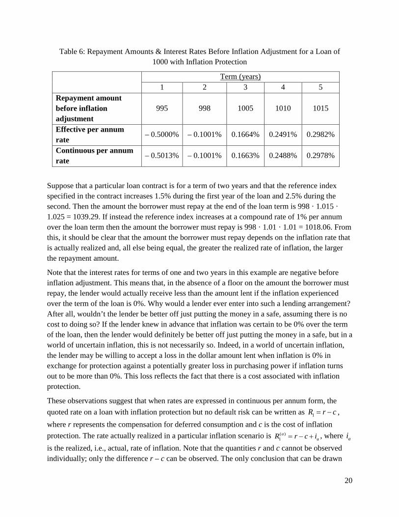
Table 6: Repayment Amounts & Interest Rates Before Inflation Adjustment for a Loan of 1000 with Inflation Protection

Term (years)

1 2 3 4 5 Repayment amount before inflation adjustment

995 998 1005 1010 1015

Effective per annum rate

– 0.5000% – 0.1001% 0.1664% 0.2491% 0.2982%

Continuous per annum rate

– 0.5013% – 0.1001% 0.1663% 0.2488% 0.2978%

Suppose that a particular loan contract is for a term of two years and that the reference index specified in the contract increases 1.5% during the first year of the loan and 2.5% during the second. Then the amount the borrower must repay at the end of the loan term is 998 · 1.015 · 1.025 = 1039.29. If instead the reference index increases at a compound rate of 1% per annum over the loan term then the amount the borrower must repay is 998 · 1.01 · 1.01 = 1018.06. From this, it should be clear that the amount the borrower must repay depends on the inflation rate that is actually realized and, all else being equal, the greater the realized rate of inflation, the larger the repayment amount.

Note that the interest rates for terms of one and two years in this example are negative before inflation adjustment. This means that, in the absence of a floor on the amount the borrower must repay, the lender would actually receive less than the amount lent if the inflation experienced over the term of the loan is 0%. Why would a lender ever enter into such a lending arrangement? After all, wouldn’t the lender be better off just putting the money in a safe, assuming there is no cost to doing so? If the lender knew in advance that inflation was certain to be 0% over the term of the loan, then the lender would definitely be better off just putting the money in a safe, but in a world of uncertain inflation, this is not necessarily so. Indeed, in a world of uncertain inflation, the lender may be willing to accept a loss in the dollar amount lent when inflation is 0% in exchange for protection against a potentially greater loss in purchasing power if inflation turns out to be more than 0%. This loss reflects the fact that there is a cost associated with inflation protection.

These observations suggest that when rates are expressed in continuous per annum form, the quoted rate on a loan with inflation protection but no default risk can be written as 1R r c= − , where r represents the compensation for deferred consumption and c is the cost of inflation protection. The rate actually realized in a particular inflation scenario is ( )

1a

aR r c i= − + , where ai is the realized, i.e., actual, rate of inflation. Note that the quantities r and c cannot be observed individually; only the difference r – c can be observed. The only conclusion that can be drawn

21

from observing that the quoted rate on a loan with inflation protection is negative is that the cost of inflation protection exceeds the compensation for deferred consumption.

3.4.2 LOANS WITHOUT INFLATION PROTECTION Loans of the type just discussed preserve the lender’s purchasing power but introduce uncertainty into the amount the borrower must ultimately repay. A borrower on a fixed income may not wish to take on this uncertainty and accordingly may be willing to pay the lender additional interest for the privilege of knowing with certainty what the repayment amount will be. In this case, the lender assumes the risk that the purchasing power of the amount lent will not be preserved and sets the repayment amounts at higher levels.

The compensation that the lender receives for assuming the risk of lost purchasing power takes two forms:

• Compensation for the loss in purchasing power that is expected over the term of the loan at the time the contract is entered into; and

• Compensation for the risk that the loss in purchasing power actually realized is greater than what was expected.

This suggests that when rates are expressed in continuous per annum form, the rate on a loan without inflation protection and with no risk of default can be written as 2 ,e uR r i i= + + where r

represents the compensation for deferred consumption, ei represents the compensation for

expected inflation, and ui represents the compensation for unexpected inflation. Comparing this formula to the formula *R r s i= + + in the case of an economy with certain inflation and noting that s = 0 when there is no risk of default, it is clear that the compensation for expected inflation 𝑖𝑖𝑒𝑒 is simply the expected rate of inflation. Moreover, it appears that when inflation rates are stable, i.e., prices in the economy increase at a steady pace, ui will be fairly small but when they

are volatile, ui could be quite large.

3.4.3 REAL AND NOMINAL INTEREST RATES The quoted interest rate on a loan with inflation protection is known as the real interest rate. The corresponding interest rate for a loan without inflation protection is known as the nominal interest rate. From the preceding discussion, we see that when rates are expressed in continuous per annum form and there is no risk of default, the real interest rate for a loan of a given term is

1R r c= − and the nominal interest rate is 2 e uR r i i= + + . The actual rate of interest earned on a

loan with inflation protection is ( )1

aaR r c i= − + .

None of the quantities r, c, ei , or ui can be observed directly. However, the difference between

the nominal and real interest rates, which is equal to 2 1 e uR R i i c− = + + , can be observed. This difference depends on the expected rate of inflation, the cost of inflation protection and the

22

compensation for unexpected inflation. Financial commentators often say that the difference between nominal and real interest rates provides an indication of the inflation rate expected by the financial market. However, from this equation, we see that this is only true when ui c+ is

small relative to ei , which can only happen when inflation rates are relatively stable and not too

close to zero. In general, the difference 2 1R R− overestimates the market’s expectation of future inflation.

As noted earlier, real rates can be negative and when this happens, it means that the cost of inflation protection is greater than the compensation for deferred consumption. Nominal rates can also be negative, at least in theory, but the circumstances under which this can occur are somewhat different. From the formula 2 e uR r i i= + + and assuming that the compensation for

unexpected inflation ui can never be negative, at least one of r or ei must be negative for the

nominal rate to be negative. Now 0ei < means that inflation is expected to be negative, i.e., prices are expected to fall over the term of the loan. When this happens, the purchasing power of money increases over time, which means that the money a borrower repays at the end of the loan term is worth more than it was at the beginning of the term. In theory, the repayment amount under such circumstances should be adjusted to account for the increased purchasing power; however, this assumes that the person with money to lend has no other alternative but to lend it to someone. In reality, the lender could just as easily put the money in safekeeping. Provided that the costs of safekeeping are not too high, this might be a better alternative. In this situation, there is no compensation for deferred consumption and the negative nominal interest rate simply represents the cost of safekeeping.

3.4.4 DECOMPOSITION OF THE INTEREST RATE WHEN DEFAULTS ARE POSSIBLE The preceding discussion assumed no risk of default. In reality, most loans have some default risk associated with them. In this situation, the interest rate on a loan of a given term can be written as *

e uR r s i i= + + + where all rates are expressed in continuous per annum form and depend on the loan term. The quantity s is known as the credit spread or alternatively the spread for credit risk. Note that *

2.s R R= − In practice, credit spreads are determined using this formula, i.e., by calculating the difference between the observed rate on the loan with default risk and the observed rate on a loan of the same term without default risk.

Credit spreads vary with loan term and the collection of spreads by loan term is known as the spread curve. Similar to yield curves, spread curves can have a variety of shapes; however, most of the time, they are upward-sloping, reflecting the fact that the longer the term of the loan, the greater the risk of default.

Unlike the situation in a world of certain inflation, credit spreads can vary with the inflation environment. When the compensation for inflation is higher than average, credit spreads are

23

often lower. All else being equal, higher inflation makes it easier for borrowers to repay debts, which in turn means that default is less likely.

4 Retail Savings and Lending Interest Rates The previous two chapters of this study note considered interest rates from a conceptual perspective and identified important determinants of interest rates including the supply and demand of money and the extent to which the purchasing power of money changes over time. In this chapter and the two that follow, we consider how interest rates arise in practice. The focus of this chapter is on interest rates associated with retail savings and lending products; rates associated with government and corporate bonds are considered in the chapter that follows. Our discussion will reveal additional factors that influence the level of interest rates including the overhead costs associated with financial intermediation, the presence or absence of embedded options or guarantees, and the liquidity of financial markets. As we will soon see, interest rates can vary greatly from one product or borrower to another and can fluctuate by material amounts over time.

4.1 BANKS AS INTERMEDIARIES BETWEEN BORROWERS AND SAVERS When the concepts of interest and supply and demand curves for money were introduced, it was implicitly assumed that borrowers and lenders are able to identify each other and enter into transactions on their own. In reality, it is very difficult for borrowers and lenders to do this without the assistance of some third party whose business it is to identify potential borrowers and lenders and match them up. The third parties who perform this function are known as financial intermediaries.

In the retail market, the most important financial intermediaries are banks and savings and loan companies. Banks and savings and loan companies accept deposits from the general public and in turn extend loans to individuals, small businesses, and corporations. For banking to work, the interest rates charged on loans must be greater than the interest rates paid on deposits; further, the difference between these rates must be sufficient to cover overhead costs and the losses on loans that go into default, as well as provide a reasonable amount of profit for owners.

In most jurisdictions, entities that accept deposits from the general public are heavily regulated at either the federal or state level to ensure that depositors’ money remains safe and is ultimately returned when promised. Banks are also regulated because of the important role they play in the payments system. In developed economies, the vast majority of payments for goods and services are made by check or using a debit or credit card, and virtually all such payments pass through one or more banks. Hence, the failure of a bank not only affects depositors of that bank but can also impede others in the economy from conducting business, particularly if the bank is large and responsible for processing a significant number of payments.

Banks and savings and loan companies are not the only financial intermediaries operating in the retail market. In recent years, alternative lenders have emerged. These lenders, many of which

24

operate online platforms only, do not accept deposits from the general public but instead raise the funds needed for lending directly from investors. Because they do not accept deposits from the general public, these companies are not regulated as banks; however, the business in which they are engaged is very similar to banking and, as a result, sometimes referred to as “shadow banking.” The growing importance of shadow banking and the risks associated with it became apparent during the financial crisis of 2008-09 when a number of alternative lenders collapsed. Without the support that comes from being part of the regulated financial system, these lenders found it difficult to raise the funds needed to continue operations; their collapse reverberated throughout the credit markets and had a negative impact on the overall economy.

Alternative payment providers that operate outside the traditional banking system have also become more prominent in recent years. Examples include PayPal, Apple Pay and Bitcoin. Most of these alternative payment providers use smartphones or the internet to process payments and rely on sophisticated encryption technology to protect a user’s identity and financial information. These companies are part of a growing number of companies, known collectively as financial technology companies or “fintech” companies for short, that use new technology to offer traditional banking services, albeit in a non-traditional way. Whether any of these financial technology companies will pose an existential threat to traditional banks remains to be seen. However, whatever form banking takes in the future, the basics of the business model are likely to stay the same: charge more interest for the loans one extends than it costs to fund them.

4.2 SAVINGS INTEREST RATES Banks and savings and loan companies offer two basic types of savings products: savings accounts, which give the customer the flexibility to withdraw any amount up to the full account balance at any time without penalty, and certificates of deposit or CDs, which require the customer to keep the money on deposit for a defined period of time (usually with a penalty for early withdrawal). Banks also offer transaction or checking accounts; however, such accounts typically pay little or no interest and hence are not considered further.

In addition to the general economic factors such as inflation discussed in the previous chapter, there are additional factors that determine the interest rate that a bank pays on savings deposits. By far, one of the most significant is the overhead cost of the bank. Full service banks that operate in many lines of business and have large networks of physical branches have much higher overhead costs than banks that operate online only and have only one or two lines of business. These higher costs must be recouped by paying savers less, charging borrowers more, or both. The difference in interest rates paid by online versus traditional banks can be substantial.

The business environment in which a bank operates also affects the interest it is willing to pay on savings products. When the demand for loans is high in a particular region of the country, banks operating in that region may be willing to pay more interest to depositors to attract the additional deposits necessary to fund the loans. This explains why the interest rates in different regions of a country, e.g., Michigan versus Texas, can sometimes be different.

25

The business strategy pursued by a bank may also affect the amount of interest it is willing to pay on savings products. For example, banks seeking to grow the size of their loan book may need to pay more interest than other banks operating in the same market to attract the deposits necessary to fund the desired growth.

Finally, the credit rating or perceived creditworthiness of a bank can affect the interest rate it must offer to attract deposits. Although most banks operating in the U.S. are insured under the FDIC7, the failure of a bank can still be costly for depositors. For example, depositors may have limited access to their funds during a wind-up of operations or may have to arrange for their accounts to be transferred to another bank. Banks that are perceived to be at greater risk of failure generally have to provide depositors some incentive to keep their money on deposit. That incentive often comes in the form of a higher rate on deposits, particularly ones that are locked in for a longer term, but could take other forms as well, such as a free checking account or discounts on selected bank services.

This is by no means a complete list of the factors that determine the interest rates that a bank pays on deposits, but it captures most of the key ones.

4.3 LENDING INTEREST RATES Banks and savings and loan companies offer lending products such as credit cards, personal loans, auto loans, and mortgages. There are three basic types of lending products:

• Those such as mortgages, auto loans, or home equity loans that are secured by property that can be seized by the lender in the event that the borrower fails to repay the full amount of the loan;

• Those such as credit cards that are not secured by any property; and • Those such as student loans or high-ratio mortgages (mortgages for which the size of the

loan is almost as large as the value of the property and there is little equity in the underlying property) that are guaranteed by a third party such as the federal government or a mortgage guaranty insurance company that agrees to cover the lender’s losses up to defined limits in the event that the borrower defaults.

These three types of lending products are known respectively as secured loans, unsecured loans, and guaranteed loans (or, more descriptively, loans with guaranteed repayment). The property that is designated as security for a secured loan is known as collateral.

In the previous chapter, we saw that the component of the interest rate that provides compensation for default risk depends on the likelihood that a borrower defaults and the extent to which recovery is possible in the event of default. In practical terms, this suggests that, in addition to the economic factors noted in that chapter, the interest rate on a loan provided by a

7 Federal Deposit Insurance Corporation, the agency of the U.S. government that insures the deposits of savers against failure of a bank. At the time of writing, the amount of coverage was 250,000 per person or legal entity per covered bank.

26

bank or savings and loan company is determined by the creditworthiness of the borrower, whether the loan is secured, unsecured or has a guarantee, and the quality and extent of any security or guarantee. All else being equal, the rate on a loan to a higher risk borrower should be higher, and the rate on an unsecured loan such as a credit card should be greater than the rate on a secured loan such as a mortgage. Similarly, the rate on a loan without a guarantee should be greater than the rate on a loan with one.

Unlike the situation for deposit products where all customers generally receive the posted rate,8 the loan rates posted by a bank are only indicative. The actual rate that a borrower pays on a loan of a given type depends on the creditworthiness of the borrower as indicated by factors such as borrower income and credit history. All else being equal, a borrower with a steady paycheck and a history of making payments on time will pay a lower rate than a borrower whose income is primarily derived from sales commissions and who has been late paying bills.

The exception to this is the rate charged on credit cards. Regulations generally prohibit credit card companies from charging different customers different rates unless a customer misses a payment on the credit card account itself, in which case the credit card company is permitted to raise the interest rate that it charges that particular customer. Of course, credit card companies are still permitted to charge different rates on different cards and will often design their cards so that higher risk borrowers prefer one type of card while lower risk ones prefer another; for example, some banks have found that cards offering cash back rewards are especially attractive to customers who pay their balance in full each month.

A bank’s prime rate is the rate it charges its best and most creditworthy customers. Very few customers are eligible to borrow money at a bank’s prime rate. However, the prime rate is generally a benchmark for the bank’s other loan rates and is useful for comparing the rates charged by one bank versus another. Banks with higher prime rates tend to have higher rates for all lending products, but not always.

By contrast, the mortgage rates posted by banks are typically higher than what a customer with good credit history and an established relationship with the bank can expect to pay. Most full service banks are willing to provide their customers discounts on posted mortgage rates in recognition of the fact that the bank that holds a customer’s mortgage is typically the bank where most of the customer’s other business is conducted and any discount provided on the mortgage rate can generally be recovered by selling the customer other high-margin products such as mutual funds or retirement savings accounts.

5 Bonds Issued by Governments and Corporations Like individuals and small businesses, governments and large corporations borrow money for a variety of reasons, from managing short-term cash flow shortfalls, e.g., when there is a mismatch 8 Some banks may offer better savings rates to customers with larger amounts on deposit or as an incentive to transfer new money into the bank. Depending on the regulatory environment in which it operates, the bank may be required to publicly disclose the offer and make it available to all customers as well as the general public.

27

in the timing of receipts and disbursements, to investing in longer-term assets such as roads and bridges, schools and hospitals, or manufacturing plants. However, the borrowing needs of governments and large corporations are much greater than those of individuals or small businesses, and can range from hundreds of millions to billions of dollars. Few if any banks have the capacity or desire to lend amounts of this size to a single borrower. Hence, governments and large corporations seeking to raise large amounts of money must generally turn to the public financial markets.

The usual way to raise money in the public financial markets is by issuing securities. There are two basic types of securities: bonds and stocks (also known as shares). Bonds are similar to the certificates of deposit issued by banks in that interest is paid to the holder of the bond at regular intervals and the face amount of the bond is repaid on a specific date, known as the maturity date; however, unlike CDs, bonds can be sold to third parties after issue and there is no guarantee that the holder of the bond will be fully repaid. By contrast, stocks represent an ownership position in the entity that issued the security and entitle the holder to a share of the entity’s profits. By issuing securities, governments and large corporations are able to raise large amounts of money in a fairly efficient way while spreading the risks associated with providing this money over a large group of investors. For obvious reasons, governments and non-profit corporations can only issue bonds, whereas profit-seeking corporations can issue either bonds or stocks.

After a bond is issued, it can be purchased or sold through an investment broker until such time that the bond matures or is redeemed by the issuer. The prices of bonds change from day to day or more frequently and depend on factors that include the creditworthiness of the issuer, the liquidity of the market, the currency in which the bond is denominated, the time until the bond matures, the expected rate of inflation, the tax treatment of interest payments, and in the case of corporate bonds, the seniority of the bond issue in a company’s capital structure. These price changes along with the natural tendency of bonds to age and hence bond terms to shorten as bonds approach maturity result in changes to bond yields.

In this chapter, we discuss the factors that affect bond prices and yields, with a particular focus on the bonds of the U.S. Treasury, state and local governments, the Government of Canada, and large multinational corporations.

5.1 ZERO-COUPON BONDS Most bonds with term greater than one year at the time of issue pay interest at regular intervals prior to maturity. In the U.S. and Canada, the usual convention is to pay interest (known as a coupon payment or just coupon) once every six months, and accordingly calculate yields based on semi-annual compounding. However, some bonds with term greater than one year pay no interest prior to maturity, i.e., the coupon rate is 0% and the holder receives the face amount of the bond at maturity. These are effectively compound interest bonds with the difference between the face amount and the price of the bond representing the amount of interest that the bondholder receives at maturity. Because they have no interest coupons, such bonds are known as zero-coupon bonds.

28

Zero-coupon bonds are typically created by an investment bank in the following way. The bank will buy a large quantity of bonds of a particular issue, remove the interest coupons from these bonds, and then sell each of the interest coupons as well as the original face amount as a separate bond. This process for creating zero-coupon bonds is sometimes referred to as stripping the coupons from a bond. For this reason, zero-coupon bonds are also known as strip bonds. Once they are created, the strip bonds associated with a particular bond issue trade separately. Hence, the yields on strip bonds of different maturities are generally different from one another; they are also generally different from the yield on the coupon bond that was used to create them in the first place.

Stripping the interest coupons from a coupon bond and trading each of the resulting strip bonds separately is a straightforward way to determine the yield curve for an entity that issues bonds infrequently and may only have a few issues outstanding. Provided that there is sufficient trading in the resulting strip bonds, the observed yields should provide a good indication of the interest rates that an issuer would have to offer on new bonds of various terms. For a given issuer, the collection of strip bond yields by term is known as the zero-coupon yield curve for that issuer.

Strip bonds are the most fundamental type of bond there is and zero-coupon yield curves the most natural type of yield curve to consider. Indeed, after a little reflection, it should be clear that every coupon bond is really just a portfolio of zero-coupon bonds with each interest coupon and the maturity amount of the bond representing a different zero-coupon bond. Hence, given the prices of a particular issuer’s strip bonds, one should be able to determine the price of any bond of this issuer, at least in theory.

With this perspective, one sees that the yield on a coupon bond is a complex weighted average of the yields on various zero-coupon bonds with the weights determined in part by the relative size of the interest coupons. When the coupon rate on an interest-paying bond is high, the interest coupons will represent more of the bond’s total cash flow and receive more weight than the maturity amount; when the coupon rate is low, the interest coupons will represent less of the bond’s total cash flow and receive less weight than the maturity amount. Since yields normally increase with term, this means that, all else being equal, the yield on a bond with a high coupon rate will generally be lower than the yield on a bond with a low coupon rate.

The fact that two coupon-bearing bonds of the same issuer with the same maturity date can have different yields presents a bit of a challenge when it comes to defining the notion of yield curve for coupon-bearing bonds. The usual convention is to define the yield for a given term to be the yield on a bond of this term that is trading at par.

5.2 U.S. TREASURY SECURITIES The most widely held and traded bonds in the world are the bonds of the federal government of the U.S. These bonds, which are issued by the Treasury Department of the U.S. government at regular intervals and collectively known as U.S. Treasury securities, are considered to be among the safest bonds in the world and are virtually free of default risk.

29

The U.S. Treasury issues two basic types of bonds: Treasury bills, which have term one year or less at issue, have no interest coupons, and are sold at a discount to maturity value; and Treasury notes/bonds, which have terms ranging from two to 30 years at issue,9 have semi-annual interest coupons, and are typically issued at or near par. Treasury bills and notes/bonds are initially sold by auction with designated banks and brokers as participants in the auction; this ensures that the initial rates offered are reasonably indicative of prevailing market conditions. They are then traded in the secondary market with the prices and yields at any given time determined by the market conditions prevailing at the time. Yields on U.S. Treasury bills are quoted using the convention described in Chapter 2 (simple discount with actual/360 day count), while yields on U.S. Treasury notes/bonds are quoted based on semi-annual compounding.

There are two types of Treasury notes, those in which the interest payments and maturity amount are fixed at issue and those in which the interest payments and maturity amount are indexed to inflation. The first type, known as nominal return bonds, are more common and have a longer history; the second type, known variously as real return bonds or inflation-indexed bonds, are less common and have only been issued by the U.S. Treasury since the 1990s. Interest payments and maturity amounts on real return bonds are calculated in a way similar to that described in the section of Chapter 3 on loans with inflation protection; the precise details of the calculation of course depend on the particulars of the bond issue. Real return bonds issued by the U.S. Treasury are known as Treasury Inflation-Protected Securities or TIPS for short.

Real return bonds are important because they provide sponsors of pension plans that have benefits indexed to inflation a mechanism for managing the risk that long-term inflation turns out to be greater than expected. The U.S. government is well positioned to assume this risk because its tax receipts are directly linked to inflation rates; indeed, as wages and prices increase, so too do the income and excise taxes it receives. However, pension plans are less well positioned to take on this risk. By purchasing real return bonds, pension plans can transfer this risk to the U.S. Treasury.

Real return bonds are also important for individual investors and retirees who are not members of a pension plan. By investing a portion of their savings in real return bonds, income-seeking investors or retirees can protect at least some of their income against the ravages of inflation, which can be substantial over time. Indeed, with only a 2% per annum inflation rate, an item that costs 100 today will cost almost 150 in 20 years, a 50% increase or equivalently a one-third loss in the purchasing power of money.

Yield information on U.S. Treasury bonds traded in the secondary market is published each business day by the U.S. Federal Reserve and is available at the website http://www.federalreserve.gov/releases/h15/. Yields are published for specified terms. Table 7 shows the actual yields published for May 10, 2016. Note that the one-year T-bill yield is slightly lower than the one-year Treasury constant maturity nominal yield; this is due to the differences 9 Those with maturities from two to 10 years are called notes, those with longer maturities are called bonds. In this note the two terms are used interchangeably as the only relevant distinction is the length.

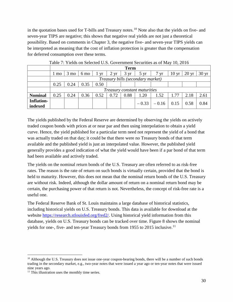
30

in the quotation bases used for T-bills and Treasury notes.10 Note also that the yields on five- and seven-year TIPS are negative; this shows that negative real yields are not just a theoretical possibility. Based on comments in Chapter 3, the negative five- and seven-year TIPS yields can be interpreted as meaning that the cost of inflation protection is greater than the compensation for deferred consumption over these terms.

Table 7: Yields on Selected U.S. Government Securities as of May 10, 2016 Term 1 mo 3 mo 6 mo 1 yr 2 yr 3 yr 5 yr 7 yr 10 yr 20 yr 30 yr Treasury bills (secondary market) 0.25 0.24 0.35 0.50 Treasury constant maturities

Nominal 0.25 0.24 0.36 0.52 0.72 0.88 1.20 1.52 1.77 2.18 2.61 Inflation-indexed – 0.33 – 0.16 0.15 0.58 0.84

The yields published by the Federal Reserve are determined by observing the yields on actively traded coupon bonds with prices at or near par and then using interpolation to obtain a yield curve. Hence, the yield published for a particular term need not represent the yield of a bond that was actually traded on that day; it could be that there were no Treasury bonds of that term available and the published yield is just an interpolated value. However, the published yield generally provides a good indication of what the yield would have been if a par bond of that term had been available and actively traded.

The yields on the nominal return bonds of the U.S. Treasury are often referred to as risk-free rates. The reason is the rate of return on such bonds is virtually certain, provided that the bond is held to maturity. However, this does not mean that the nominal return bonds of the U.S. Treasury are without risk. Indeed, although the dollar amount of return on a nominal return bond may be certain, the purchasing power of that return is not. Nevertheless, the concept of risk-free rate is a useful one.

The Federal Reserve Bank of St. Louis maintains a large database of historical statistics, including historical yields on U.S. Treasury bonds. This data is available for download at the website https://research.stlouisfed.org/fred2/. Using historical yield information from this database, yields on U.S. Treasury bonds can be tracked over time. Figure 8 shows the nominal yields for one-, five- and ten-year Treasury bonds from 1955 to 2015 inclusive.11

10 Although the U.S. Treasury does not issue one-year coupon-bearing bonds, there will be a number of such bonds trading in the secondary market, e.g., two-year notes that were issued a year ago or ten-year notes that were issued nine years ago. 11 This illustration uses the monthly time series.

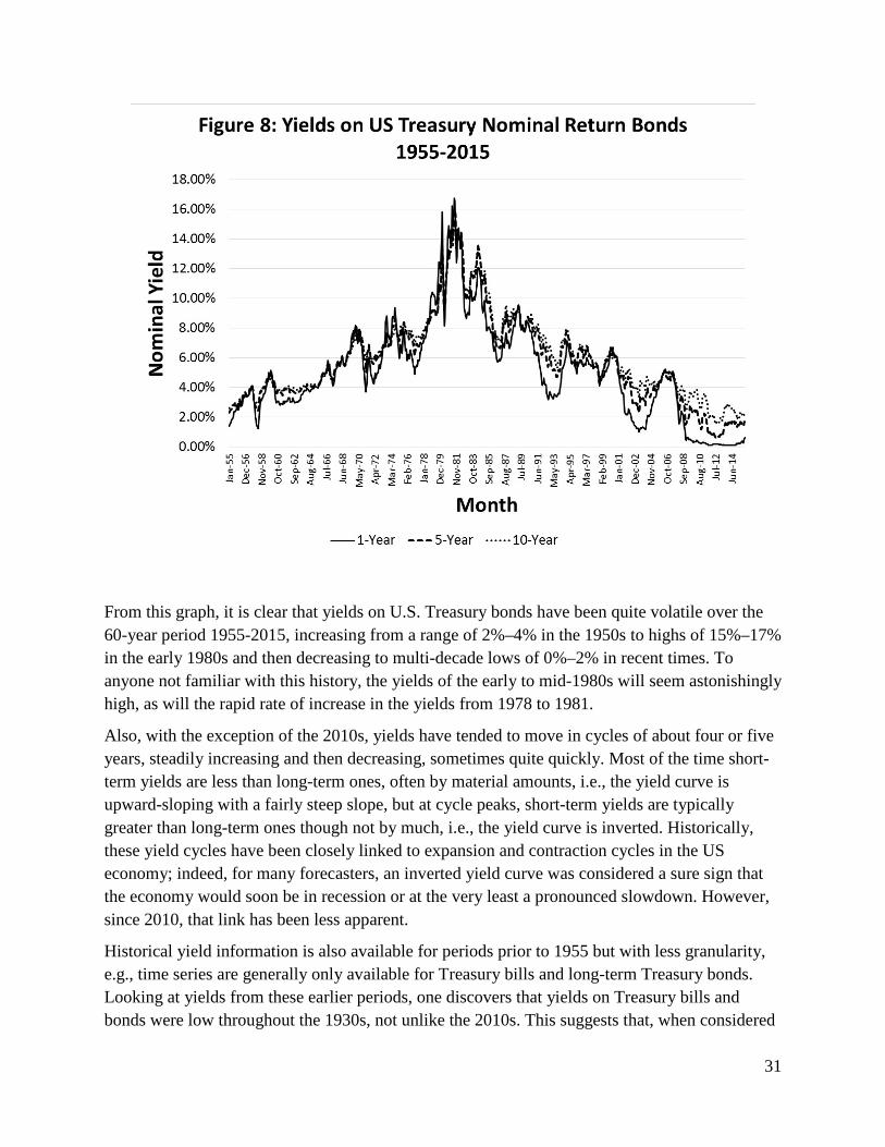
31

From this graph, it is clear that yields on U.S. Treasury bonds have been quite volatile over the 60-year period 1955-2015, increasing from a range of 2%–4% in the 1950s to highs of 15%–17% in the early 1980s and then decreasing to multi-decade lows of 0%–2% in recent times. To anyone not familiar with this history, the yields of the early to mid-1980s will seem astonishingly high, as will the rapid rate of increase in the yields from 1978 to 1981.

Also, with the exception of the 2010s, yields have tended to move in cycles of about four or five years, steadily increasing and then decreasing, sometimes quite quickly. Most of the time short-term yields are less than long-term ones, often by material amounts, i.e., the yield curve is upward-sloping with a fairly steep slope, but at cycle peaks, short-term yields are typically greater than long-term ones though not by much, i.e., the yield curve is inverted. Historically, these yield cycles have been closely linked to expansion and contraction cycles in the US economy; indeed, for many forecasters, an inverted yield curve was considered a sure sign that the economy would soon be in recession or at the very least a pronounced slowdown. However, since 2010, that link has been less apparent.

Historical yield information is also available for periods prior to 1955 but with less granularity, e.g., time series are generally only available for Treasury bills and long-term Treasury bonds. Looking at yields from these earlier periods, one discovers that yields on Treasury bills and bonds were low throughout the 1930s, not unlike the 2010s. This suggests that, when considered

32

in the context of a longer historical period, the yield environment of the 2010s may not be as unusual as it at first appears from the graph in Figure 8.

5.3 STATE AND LOCAL GOVERNMENT BONDS IN THE UNITED STATES The federal government of the U.S. is not the only level of government that issues bonds in the U.S. State and local governments also issue bonds, although the extent to which a particular state or municipality may do so is sometimes limited by the state’s constitution or laws; for example, a state may have in place a balanced budget law, which is a type of law that requires the state government to balance its budget each fiscal year and severely limits its ability to borrow money to meet current expenditures. One of the main reasons that state and local governments issue bonds is to finance the construction and maintenance of long-term infrastructure such as municipal water systems, schools and hospitals, and roads and bridges.

There are two basic types of bonds issued by state and local governments: revenue bonds and general obligation bonds. Revenue bonds are bonds that are backed by revenues generated from a dedicated source such as the tolls levied on drivers using a particular road or bridge, or the charges levied on homeowners for municipal water service. General obligation bonds are bonds that are backed by the general taxing authority of the state or local government.

Unlike the bonds of the U.S. Treasury, the bonds of state and local governments are not free of default risk. Indeed, the governments of some states and municipalities have gotten into financial difficulty in the past and in some cases even gone bankrupt; notable examples include New York City in the 1970s, Orange County, California in the 1990s, and more recently, the city of Detroit. Hence, all else being equal, the yields on state and local government bonds should be higher than the yields on US Treasury bonds of the same term, with the yield premium being greater for less creditworthy issuers.

However, state and local government bonds have a feature that can result in their yields being lower than they otherwise would be. Provided that a number of conditions are met, the interest paid on certain types of bonds issued by state or local governments in the U.S. can be tax free or taxable at a preferred rate. In this context, tax free means that the person or entity receiving the interest payments does not have to pay income tax on the interest received, while taxable at a preferred rate means that the tax rate is lower than it would be for other types of income such as wages.

The tax-free or tax-preferred status of these bonds make them attractive for income-seeking investors such as retirees. State and local governments are aware of this and typically set the coupon rate for these bonds at a level that is lower than would otherwise be required by investors.

5.4 GOVERNMENT BONDS IN CANADA Up until now, we have considered interest rates without reference to the currency in which the particular savings or lending product or bond is denominated, or as in the discussion of U.S.

33

Treasury securities, tacitly assumed that the underlying currency is U.S. dollars. However, as we broaden the scope of our discussion to include bonds issued outside the U.S., it becomes necessary to consider currency more explicitly. Outside the U.S., financial transactions including transactions involving the borrowing or lending of money are typically conducted in the currency of the country where the transaction takes place. For example, transactions that take place in Great Britain are typically conducted in British pounds (also known as pound sterling) and transactions that take place in Canada are typically conducted in Canadian dollars.

Like the U.S. government, the Government of Canada issues bonds of various terms, ranging from Treasury bills with a duration of 91 days at issue to long-term Treasury bonds with a maturity of 30 years at issue. Most of these bonds are issued in Canadian dollars, but some are issued in U.S. dollars, mainly to meet the needs of U.S. and other international investors who are interested in buying the bonds of the Government of Canada but do not wish to be exposed to fluctuation in the value of the Canadian dollar.

The Canadian dollar, like the currencies of most other industrialized nations with well-developed economies, is a floating currency, which means that its value against the U.S. dollar and other currencies continually changes based on the supply and demand for Canadian dollars in international currency markets. When demand for Canadian dollars is high as generally occurs when there is a lot of demand for Canadian assets or the goods and services produced by companies located in Canada, the Canadian dollar increases in value. When demand is low, the Canadian dollar decreases in value. Currency fluctuation is an important consideration for international investors because their return on an investment depends not only on the return in the local currency but also on the extent to which the value of the local currency changes over the life of the investment compared to the investor’s own currency.

The Government of Canada has issued bonds for over a century and has an unbroken record of repayment. To U.S. investors, Government of Canada bonds are almost as safe as U.S. Treasuries. Hence, the yields on Government of Canada bonds that are denominated in U.S. dollars tend to be very similar to the yields on U.S. Treasury bonds; the slight differences that do exist are attributable to the fact that bonds issued by the Government of Canada trade less frequently and in lower volumes than U.S. Treasuries. However, the yields on Government of Canada bonds denominated in Canadian dollars can be quite different. The reason is that the yields on bonds denominated in Canadian dollars are primarily determined by the level of economic activity in Canada, including the overall supply and demand for Canadian dollars, while the yields on bonds denominated in U.S. dollars are primarily determined by the state of the U.S. economy.

For an investor based in Canada, the yields on the (nominal return) bonds of the Government of Canada are considered to be the risk-free rates, in the same way that the yields on the nominal return bonds of the U.S. Treasury are considered the risk-free rates for U.S.-based investors. Provided that the bonds of the Government of Canada are held to maturity, the rates of return on

34

these bonds, measured in local currency, are virtually certain. Hence, the notion of risk-free rate depends on both the term of the investment and the currency in which it is denominated.

Similar to the U.S., the governments of Canadian provinces and municipalities also issue bonds; however, these bonds are not free of default risk. Hence, the yields on the bonds of Canadian provinces and municipalities are higher than the yields on bonds of the Government of Canada.

5.5 CORPORATE BONDS Corporations issue bonds for reasons similar to governments, e.g., from managing short-term cash flow shortfalls to investing in longer term assets such as manufacturing plants, mines and oil wells. However, the frequency with which corporations issue bonds and the extent to which these bonds are traded in the secondary market is much different than it is for governments. In general, the bonds of corporations trade much less frequently than the bonds of governments. In fact, for some issues of corporate bonds, there may be little or no trading at all.

Investment brokers maintain inventories of the more actively traded corporate issues for purchase or sale. An example of the type of information that an investment broker would make available to clients is provided in Table 8.

Table 8: Selected Corporate Bond Offerings as of May 17, 2016

Coupon Maturity

Offer Quantity (1000s)

Bid Yield

Bid Price

per 100

Ask Price

per 100 Ask

Yield Type Rating ABC Grocery

6.65% 11/08/2027 44 3.7073% 127.285 129.882 3.4691% Corp BBBm 6.45% 02/09/2028 1000 3.7571% 125.337 127.943 3.5195% Corp BBBm 6.50% 01/22/2029 1000 3.9047% 125.743 128.445 3.6720% Corp BBBm 6.54% 02/17/2033 1000 4.3327% 126.083 129.142 4.1140% Corp BBBm

BCD Telecom 0.00% 02/26/2028 430 63.956 3.8330% Corp Al 6.55% 05/01/2029 88 3.8535% 127.284 130.035 3.6231% Corp Al 4.35% 12/18/2045 1000 4.4275% 98.725 102.183 4.2199% Corp Al

EFG Pipeline 0.00% 07/24/2029 260 52.756 4.9120% Corp BBBh 7.20% 06/18/2032 393 4.9254% 125.056 127.965 4.7014% Corp BBBh 5.75% 09/02/2039 17 4.9203% 111.417 115.424 4.6572% Corp BBBh

PIP Pipeline 4.75% 04/30/2043 107 5.3239% 91.834 94.848 5.1038% Corp BBBl

ZAP Electric 6.93% 06/01/2032 305 3.5192% 141.519 144.800 3.3071% Corp Ah 6.59% 04/22/2043 1000 3.7093% 148.786 153.185 3.5174% Corp Ah 4.00% 12/22/2051 785 3.7618% 104.648 108.719 3.5655% Corp Ah

35

Note that the bid price of a bond is the price that the investment broker is willing to pay to buy the bond from the customer while the ask price is the price at which the investment broker is willing to sell the bond to the customer; for obvious reasons, the bid price should always be lower than the ask price. The bid yield is the yield that corresponds to the bid price and the ask yield is the yield that corresponds to the ask price. Since the bid price is always lower than the ask price, the bid yield will always be greater than the ask yield.

The difference between the bid and ask yields for a particular bond issue is known as the bid-ask spread and is a measure of the liquidity of the issue. Liquidity refers to the ease with which it is possible to buy or sell a particular bond and the costs associated with doing so. When a bond is purchased and sold less frequently, brokers who maintain an inventory of the bond issue generally require customers to pay more to purchase it and they offer less to buy it back from them. Doing so protects the broker against sudden changes in the overall market, in particular, a sudden drop in the prices of all bonds. Hence, when a bond is purchased and sold less frequently, the bid yield is generally higher, the offer yield lower, and the bid-ask spread greater. From Table 8, note that the bid-ask spread for the ZAP Electric bond maturing on April 22, 2043 is 0.19% while for the PIP Pipeline bond maturing on April 30, 2043 (eight days later), it is 0.22%, which suggests that the ZAP Electric bond is slightly more liquid than the PIP Pipeline bond. The bid-ask spread for a typical U.S. Treasury or Government of Canada bond would be even lower.

The rating associated with a bond issue provides an indication of the likelihood of issuer default and the recovery one can expect in the event of default. All else being equal, the higher the rating, the lower the likelihood of default and the higher the likely recovery in the event of default; hence, higher rated bonds typically have lower yields. Ratings are generally assigned using letters of the alphabet, where A represents a higher rating than B, AA a higher rating than A, and so on; these rating classes are often subdivided by affixing a suffix such as l, m, h (low, medium, high) or simply +/-. The ratings provided by investment brokers generally come from an independent credit rating agency that specializes in rating bond issues. Different rating agencies use different rating criteria and alphabetical schemes, but the ratings assigned by different agencies tend to be quite similar.

Recovery on a bond in the event of default is determined in part by the seniority of the bond in the issuer’s capital structure. Seniority refers to the order in which the holders of a corporation’s securities would be paid in the event of liquidation; holders of the more senior issues are paid first while holders of common equity are paid last. Corporations frequently issue bonds with different seniorities. Some bond issues will be secured by specific assets; others will be unsecured but senior to all other unsecured debt; and still others will be subordinated, i.e., lower than other debt but still higher than common equity or preferred shares. All else being equal, the price of a corporation’s more senior debt should be higher and the yield lower than the corporation’s less senior debt. A bond’s seniority is often taken into consideration when a credit

36

rating is assigned to a bond issue, but not always; the issuer’s overall creditworthiness is still usually the dominant factor.

Finally, many corporate bonds have provisions that give the issuer or the holder the right to redeem the bond before maturity subject to particular conditions being met. These provisions can be quite valuable to either the issuer or the holder of the bond and accordingly will affect the bond’s price and yield. There are two basic types of early redemption provisions: calls and puts. A call provision is a provision that allows the bond’s issuer to redeem (“call”) the bond before maturity at a particular price, usually above par, that is defined at the time of issue. A put provision is a provision that allows the bond’s holder to sell (“put”) the bond back to the issuer before maturity at a particular price, usually below par, that is defined at the time of issue.

Call provisions are valuable to bond issuers because they enable issuers to redeem their outstanding bonds when interest rates drop below particular levels and then issue new bonds at the lower rates prevailing at that time. Indeed, as interest rates drop, bond prices generally rise, all else being equal, and so when interest rates drop to the level where a bond’s price reaches the price at which it can be redeemed by the issuer, the issuer is generally better off redeeming the bond and issuing a new one than continuing to make interest payments on the existing bond. Early redemption enables the issuer to save on future interest costs but has an adverse effect on the bondholder, who will not receive the higher interest payments that would have otherwise been made. Bond purchasers must be compensated for this possibility by paying a lower price or, equivalently, receiving a higher yield. Hence, all else being equal, a bond with a call provision should have a higher yield than a bond without the call provision.

Put provisions are valuable to bondholders but potentially costly to issuers. Indeed, when interest rates are rising and bond prices falling, a put provision enables the bondholder to redeem the bond and purchase a new bond at a higher rate; however, if the bondholder elects to do this, the issuer must have the funds available to repay the bondholder or else issue a new bond and pay higher interest costs going forward. Hence, all else being equal, a bond with a put provision should have a lower yield and higher price than a bond without the put provision.

In addition to liquidity, issuer creditworthiness, seniority, and the presence or absence of call or put provisions, the prices and yields on corporate bonds are determined by the same factors that affect the prices and yields of risk-free government bonds, e.g., currency, term and inflation. Like governments, corporations frequently issue bonds in more than one currency. Although corporations that are based in a single country generally issue bonds in the currency of that country, corporations whose revenues are linked to the currency of a specific country will often issue bonds in that currency instead; examples include multinational corporations and commodity producers such as oil and gas exploration and refining companies and mining companies whose products are priced in U.S. dollars regardless of where the company’s operations happen to be located.

Finally, it is worth noting that in spite of what was suggested in Chapter 3, the spread between a corporate bond and a risk-free government bond of the same term and currency may or may not

37

provide a good indication of the incremental compensation for credit risk for that term and currency. For a bond without any embedded options, e.g., put or call provisions, the spread probably provides a reasonable estimate of the compensation for credit risk; however, for a bond with one or more embedded options or one that is denominated in a currency that is different from the investor’s preferred currency, this need not be so. In the latter case, the spread is a combination of the compensation for credit risk, the compensation or cost of embedded options, and if appropriate, the compensation for assuming currency risk.

6 The Role of Central Banks We conclude this study note with a brief discussion of the role of central banks and how their actions can influence the general level of a country’s interest rates.

A central bank is a special type of bank that acts as a banker to the commercial banks that are authorized to conduct business in a given country and facilitates the movement of money throughout that country’s financial system. Today, virtually all industrialized countries with well-developed economies have a central bank; however, this was not always the case.

The form, mandate and activities of a country’s central bank vary from one country to another. In some countries, the central bank has broad responsibilities, including management of the economy, control of the currency and supervision of the banks; in other countries, the central bank’s role is more limited and may not even include issuance of the country’s currency. The two core functions of any central bank are to facilitate the operation of a country’s payment system and act as a lender of last resort for banks that are authorized to do business in the country.

6.1 OPERATION OF THE PAYMENT SYSTEM In modern well-developed economies, the payment system works so well that most people take it for granted and in fact may not even be aware that it is there. One goes to the grocery store, uses one’s debit card to make payment, and automatically assumes that the payment will be accepted as long as there are sufficient funds in the bank account linked to the card. One hires a landscaper, writes the landscaper a check, and automatically assumes that the landscaper’s bank will deposit the check to the landscaper’s bank account even if the landscaper deals with a different bank. One goes to work, does one’s job, and automatically assumes that come payday, one’s paycheck will be deposited to one’s bank account even if the bank one deals with is different from one’s employer.

Each of these seemingly simple transactions involves a number of different and unrelated parties. For example, in the case of the grocery store transaction, there is your bank, the grocery store’s bank, the bank that operates the debit terminals used by the grocery store, a national credit card issuer like Visa or MasterCard if the credit card issuer’s logo appears on the debit card, and possibly a number of other intermediaries. For the transaction to be successful and completed in real time, each of the parties involved needs some assurance that the parties they happen to be

38

dealing with will be able to fulfill their obligations when all accounts are settled at the end of the day (or whenever the accounts are ultimately settled). The central bank provides this assurance by being available to step in and make good on the obligations of the banks acting as intermediaries in the transaction in the unlikely event that one or more of them is unable to do so.

The central bank is able to do this because, as part of the privilege of being granted the authority to operate a bank, banks must maintain a specified amount of money on deposit with the central bank at all times. The amount of money that a given bank must maintain on deposit at the central bank is known as the bank’s reserve requirement. In general, each bank has a different reserve requirement and this reserve requirement changes from one day to the next depending on factors such as the amount of money customers have on deposit at the bank, the volume of transactions processed by the bank in a typical day, and the importance of the bank in the overall payment system. The actual amount of money that a bank has on deposit at the central bank, which necessarily will be greater than the bank’s reserve requirement, is known simply as the reserve.

The reserve amounts on deposit at the central bank provide the central bank the means to make good on a bank’s obligation. In the unlikely event that a bank is unable to fulfill its obligations under a particular transaction, the central bank can simply withdraw the money from the bank’s reserve account and complete the transaction in place of the bank. The reserve accounts also provide an efficient way of moving money from one bank to another. Rather than each bank having to maintain an account with every other bank operating in the country, banks can simply transfer money back and forth between reserve accounts at the central bank.

The actual functioning of the payment system is more complicated than what this suggests. However, this description should still give one an appreciation of the important role central banks play in facilitating payments.

6.2 LENDER OF LAST RESORT The other core function of a central bank is to act as a lender of last resort for banks that are authorized to do business in the particular jurisdiction. This function is critical to maintaining confidence in the financial system.

The public has become accustomed to thinking that the money they have on deposit in checking and savings accounts can be withdrawn at any time and, in the ordinary course of business, a bank should have little difficulty fulfilling a customer’s wishes in this regard. However, if every customer of the bank decided to withdraw the money they had on deposit at the bank and if all these requests came at the same time, the bank would be unable to honor them all for the simple reason that, at any given time, most of the money on deposit with the bank is lent to other customers and hence not immediately available. If all the money deposited with the bank were available all of the time, the bank would have no way of generating the income needed to pay interest on savings accounts or even cover the overhead associated with operating a bank, and would then have to charge customers for the privilege of keeping their money on deposit.

39

The central bank provides a backstop to banks that are experiencing higher than normal withdrawals and in so doing ensures that the public’s confidence in the bank’s ability to honor withdrawal requests from its customers is maintained. The central bank does this by lending the bank whatever it needs to meet customer withdrawal requests and using the loans on the bank’s balance sheet as security. Provided that the loans on the bank’s balance sheet are of good quality, the central bank will be reasonably confident in the bank’s ability to repay the amounts lent when the period of higher than normal withdrawals passes and should have no hesitation lending the bank the funds it needs.

Of course, a bank experiencing higher than normal withdrawals could turn to its peers for assistance rather than the central bank and, in practice, this is what often happens. However, the difference between the central bank and the bank’s peers is that the central bank is always willing and able to perform this function, even when the bank’s peers are not. It is for this reason that the central bank is referred to as the lender of last resort.

One may wonder where the central bank gets the money to lend to banks that are experiencing higher than normal withdrawals. There are two main sources. The first is the reserve accounts that all banks are required to maintain with the central bank. The money in these accounts is effectively cash. All the money in all the reserve accounts is available to support a bank that is experiencing higher than normal withdrawals. The second is currency that the central bank issues itself. Provided that the central bank has the authority to issue currency, it can issue whatever amount of cash is needed to support a bank that is experiencing higher than normal withdrawals. Of course, if the central bank does not have the authority to issue currency and a large number of banks experience higher than normal withdrawals at the same time, then the central bank may only be able to provide limited support. In such circumstances, limits are likely to be imposed on the amount each customer can withdraw over a given period of time.

6.3 THE UNITED STATES FEDERAL RESERVE BANK SYSTEM12 The central bank of the U.S. has a tripartite structure, which consists of a Board of Governors, 12 regional reserve banks, and a committee, known as the Federal Open Market Committee, that sets policy with respect to the central bank’s capital market activities such as the purchase or sale of bonds issued by the U.S. Treasury. Hence, the central bank of the U.S. is really a system of banks and accordingly is called the Federal Reserve System.

The Federal Open Market Committee, also known as the FOMC, is responsible for setting policy with respect to the central bank’s capital market activities. The most visible way it does this is through setting a target for what is known as the federal funds rate.

The federal funds rate is the interest rate at which banks with excess reserve funds at their District’s Federal Reserve Bank lend these funds to other banks. In the normal course of conducting business, a bank may find that at the end of a given day, the funds it has on deposit at 12 The information on the structure and mandate of the Federal Reserve provided in this section was obtained from the Federal Reserve’s website (http://www.federalreserve.gov/aboutthefed/structure-federal-reserve-banks.htm).

40

its reserve bank are insufficient to meet its reserve requirements for that day; borrowing the necessary funds overnight from a bank that has more funds in its reserve account than it needs is a simple and efficient way for the bank to meet its reserve requirements. Through the buying and selling of Treasury bills in the secondary market, the 12 reserve banks are able to influence the level of the federal funds rate and ensure that on any given day the federal funds rate is close to the target set by the Federal Open Market Committee.

The federal funds rate is not the same as the rate at which banks can borrow directly from the Federal Reserve, e.g., to manage higher than normal withdrawals from customers. The rate at which banks can borrow money directly from the Federal Reserve is known as the discount rate. Banks typically prefer to borrow from their peers rather than directly from the Federal Reserve because doing so sends a signal to the market that the bank is creditworthy and recognized as such by its peers.

Through its setting of the federal funds rate and other capital market activities, the FOMC is able to influence the general level of interest rates in the economy and the overall level of economic activity. For example, when the FOMC increases the target level of the federal funds rate, it makes it more expensive for banks to run a shortfall in their reserve accounts. As a result, banks have an incentive to keep more money on deposit at their reserve bank and underwrite fewer loans. This has the effect of shifting the supply curve for money. Absent a corresponding shift in the demand curve, the price of money, i.e., interest rates, will increase.

Conversely, when the FOMC decreases the target level of the federal funds rate, it makes it cheaper for banks to run a shortfall in their reserve accounts and provides them an incentive to underwrite a greater number of loans. This has the effect of shifting the supply curve for money in the opposite direction and, all else being equal, decreasing the level of interest rates charged on loans.

The FOMC’s activities, which include setting the target level for the federal funds rate, are generically referred to as setting monetary policy. Under the current provisions of the Federal Reserve Act, the Federal Reserve is to conduct monetary policy in a way that promotes maximum employment, stable prices, and moderate long-term interest rates. These goals are not mutually exclusive but at times they may conflict with one another. For example, in order to promote maximum employment, it may at times be necessary to set interest rates at levels that are lower than the level needed to keep prices stable over the long term. However, when prices are increasing at a faster rate than is consistent with stable prices, it may be necessary to set interest rates at levels that are higher than the long-term equilibrium value even if that means accepting a temporarily higher level of unemployment.

The actual workings of the Federal Reserve System are considerably more complex than discussed here and include additional activities such as the supervision of member banks and the issuance of U.S. dollars. However, the discussion presented here should still give one an appreciation of the important role that the Federal Reserve System plays in the U.S. economy and the determination of interest rates.