This article was downloaded by: [The University of British Columbia]On: 10 October 2014, At: 22:54Publisher: RoutledgeInforma Ltd Registered in England and Wales Registered Number: 1072954Registered office: Mortimer House, 37-41 Mortimer Street, London W1T 3JH,UK

The Journal of North AfricanStudiesPublication details, including instructions for authorsand subscription information:http://www.tandfonline.com/loi/fnas20

Determinants of foreign directinvestment in Sudan: aneconometric perspectiveOmer Ali Ibrahim a & Hisham Mohamed Hassan aa Department of Econometrics and Social Statistics,Faculty of Economic and Social Studies , University ofKhartoum , P.O. Box 321 , Khartoum , SudanPublished online: 16 Jul 2012.

To cite this article: Omer Ali Ibrahim & Hisham Mohamed Hassan (2013) Determinantsof foreign direct investment in Sudan: an econometric perspective, The Journal of NorthAfrican Studies, 18:1, 1-15, DOI: 10.1080/13629387.2012.702013

To link to this article: http://dx.doi.org/10.1080/13629387.2012.702013

PLEASE SCROLL DOWN FOR ARTICLE

Taylor & Francis makes every effort to ensure the accuracy of all theinformation (the “Content”) contained in the publications on our platform.However, Taylor & Francis, our agents, and our licensors make norepresentations or warranties whatsoever as to the accuracy, completeness, orsuitability for any purpose of the Content. Any opinions and views expressedin this publication are the opinions and views of the authors, and are not theviews of or endorsed by Taylor & Francis. The accuracy of the Content shouldnot be relied upon and should be independently verified with primary sourcesof information. Taylor and Francis shall not be liable for any losses, actions,claims, proceedings, demands, costs, expenses, damages, and other liabilitieswhatsoever or howsoever caused arising directly or indirectly in connectionwith, in relation to or arising out of the use of the Content.

This article may be used for research, teaching, and private study purposes.Any substantial or systematic reproduction, redistribution, reselling, loan, sub-

licensing, systematic supply, or distribution in any form to anyone is expresslyforbidden. Terms & Conditions of access and use can be found at http://www.tandfonline.com/page/terms-and-conditions

Dow

nloa

ded

by [

The

Uni

vers

ity o

f B

ritis

h C

olum

bia]

at 2

2:54

10

Oct

ober

201

4

Determinants of foreign direct investmentin Sudan: an econometric perspective

Omer Ali Ibrahim∗ and Hisham Mohamed Hassan

Department of Econometrics and Social Statistics, Faculty of Economic and Social Studies, University of Khartoum,

P.O. Box 321, Khartoum, Sudan

The paper explores the determinants of foreign direct investment (FDI) in Sudan over the period(1970–2010). The study considers the market size, inflation rate, exchange rate, indirect taxes,trade openness, and investment incentive policy as factors influencing FDI. The study uses thecointegration and error-correction techniques to identify the short- and long-run dynamics ofthe FDI determinants. The Johansen cointegration test statistics indentify four cointegratingrelations among the series, which implies an existence of long-run relationship among the FDIdeterminants. The results of the long-run FDI equation indicate that FDI flows in Sudan areinfluenced by the market size, inflation rate, exchange rate, and investment incentive policy.The error-correction term suggests that approximately 17% of total disequilibrium in FDIflows was being corrected each year. Moreover, Granger causality results show that there is aunidirectional causality running from each of the exchange rate, investment incentive policy,and the market size to FDI.

Keywords: FDI; cointegration; Granger causality; error correction; Sudan

1. Introduction

There is a growing awareness of the importance of foreign direct investment (FDI) to the devel-

oping countries and emerging economies. The FDI is not only supplementing their low saving

rates but also has the potential for providing a package of resources, including technology, man-

agement practices and assured markets (Romer 1993; World Bank 1999; Crespo and Fontoura

2007). It has also been widely documented that there is a correlation between good macroeco-

nomic policies and political stability and attraction of FDI (Mwilima 2003; Ok 2004; Baniak,

Cukrowski, and Herczynski 2005; Dupasquier and Osakwe 2005).

In their efforts to make benefits of the FDI spillovers, most developing countries have under-

taken economic reforms in early 1980s, and designated incentives policies to attract FDI. As a

result, the annual inflow of FDI to the developing countries has increased substantially from $24

billion (24% of total foreign investment) in 1990 to almost $178 billion (61% of total foreign

investment) in 2000 and amounted to $574 billion in 2010 (UNCTAD 2011).

∗ Corresponding author. Department of Econometrics and Social Statistics, Faculty of Economic and Social Studies, Uni-

versity of Khartoum, B.O Box 321, Sudan. Email: omerai@hotmail.com

# 2013 Taylor & Francis

The Journal of North African Studies, 2013

Vol. 18, No. 1, 1–15, http://dx.doi.org/10.1080/13629387.2012.702013

Dow

nloa

ded

by [

The

Uni

vers

ity o

f B

ritis

h C

olum

bia]

at 2

2:54

10

Oct

ober

201

4

Sudan represents one of the successful stories among the developing countries that managed

to attract substantial FDI (Khondoker and Kalirajan 2010). The strategic location of the country

in the horn of Africa, linking both Arab and Africa countries, the huge oil and mining reserves,

and the great animal resources and agricultural potential,1 played as pulling factors. Moreover,

the economic reforms that Sudan has introduced in early 1990s, the amendments of the Invest-

ment Encouragement Act of 1995, the exploration of the oil in 1999, and the signing of the Com-

prehensive Peace Agreement in 2005 that ended one of the longest civil war in Africa, all have

created a conducive environment for attracting FDI. Accordingly, the inflows of FDI to Sudan

have increased from US$119 million in the period 1990–2000 to US$ 2.31 billion in 2005 and

US$2.53 billion in 2008, while FDI stock stands as US$16.3 billion in 2008, representing 28.1%

of the GDP (UNCTAD 2009). Also, according to the Arab Investment and Export Credit Guar-

antee Corporation statistics in 2010, the total inter-Arab investment to Sudan during the period

1995–2010 has amounted to US$ 23.3 billion, with Sudan occupying the second recipient

country following Saudi Arabia. Most of the FDI flows to Sudan originated from the Asian

countries mainly China, Malaysia, and India in addition to Arab countries such as Saudi

Arabia, United Arab Emirates, Qatar, and Kuwait. Due to these flows, Sudan has achieved a

high and sustained growth of 9% during the period 2005–2007, being described as one of the

fastest growing economies on the Continent (World Bank, Sudan CMU 2008); despite the

American economic sanction imposed on Sudan since 1997.

There are many challenges facing the FDI in Sudan, investors always expressed their concern

about instability in macroeconomic polices, and the bureaucratic investment procedures related

to investment licensing, granting land, etc. (Ministry of Cabinet Affairs 2010). Another chal-

lenge is related to the political instability resulting from the internal conflicts in Darfur and

Southern Kordofan, which remained as a major concern to the international community as

well. It is generally believed that had Sudan strengthened macroeconomic management,

resolved its internal conflicts, and improved relationships with the international community;

it could have attracted more FDI particularly from the Western countries and sustained more

growth.

Hence, the main questions of this paper are why Sudan has managed to attract substantial FDI

despite its political instability and the tense relationship with the international community. What

factors explain the good performance of the FDI inflow in Sudan? Is it due to the economic

endowments of the country, or is it due to the incentives provided in the Investment Encourage-

ment Act of the country.

The objective of this paper is to empirically explore the determinants of FDI in Sudan, over

the period (1970–2010) by identifying the fundamental factors that drive FDI behaviour. The

study will develop an econometric model that will assess the environment for the FDI in

Sudan and examine causal links between the different determinants.

The paper is organised as follows. Section 2I presents a review of the empirical literature on

the FDI determinants; Section 3 describes the methodology; Section 4 provides empirical results

and discussion, and Section 5 is a conclusion and policy recommendations.

2. Empirical literature on FDI determinants

There is abundant literature on empirical FDI determinants. Khondoker and Kalirajan (2010)

studied the determinant of FDI in 68 low-income and lower-middle income developing

countries using panel data. Their study concluded that countries with larger GDP and high

GDP growth rate, higher proportion of international trade, and with more business friendly

O.A. Ibrahim and H.M. Hassan2

Dow

nloa

ded

by [

The

Uni

vers

ity o

f B

ritis

h C

olum

bia]

at 2

2:54

10

Oct

ober

201

4

environment are more successful in attracting FDI. The study highlighted a few countries,

such as China, India, Nigeria, and Sudan are the major FDI recipient countries. In contrast,

Edwards (1990) and Jaspersen, Aylward, and Knox (2000) found that real GDP per capita to

have a negative effect on FDI.

China, being the second largest FDI recipient in the last years, has been of interest for research

for many studies. Using primary data of 22 firms operating in China, Ali and Guo (2005) show

that market size is a major factor for attracting FDI in China, especially for US firms, while low

labor costs is the main factor for local, export-orientated, Asian firms. Others attribute the

success of China in attracting FDI to the location advantages, Zhang (2000) and Wei and Liu

(2001). Yunshi and Jing (2005) identified factors such as preferential foreign investment pol-

icies, inexpensive labour, increasing purchasing power, and improving investment environment,

especially after entry into the World Trade Organization (WTO) in 2001, as the main factors

behind China being the favourite destination for global investment.

Kinda (2010), Swain and Wang (1997) and Liu et al. (1997) found that there was a posi-

tive relationship between the relatively cheap labour in China and inward FDI. Contrary to

these findings, Schneider and Frey (1985) found the opposite. Quazi and Mahmud (2004)

used a model with a panel data for the period 1995–2000 for investigating the factors

driving FDI in five countries in South Asia: Bangladesh, India, Nepal, Pakistan, and Sri

Lanka. The study emphasised the positive role of the economic freedom, economic openness,

economic prosperity, human capital, and incremental lagged changes in attracting FDI to

South Asia, while political instability contributes negatively to FDI attraction. Also, Swain

and Wang (1997) and Liu et al. (1997) confirmed the negative role of the political instability

in the case of China.

Naeem and Azam (2005) used time series data for the period 1970–2000 for Pakistan and

found the main economic factors to be market size, domestic investment, trade openness, indir-

ect taxes, inflation, and external debt. Azam and Lukman (2008) investigated the economic

factors affecting FDI inflow into Pakistan, India, and Indonesia using secondary data from

1971 to 2005. The study used a regression model and revealed that market size, external debt,

domestic investment, trade openness, and physical infrastructure are the important economic

determinants of FDI in these countries.

Regarding the role of real exchange rate on FDI, the evidence is mixed. Blonigen and Feenstra

(1996) and Ang (2008) demonstrated a negative correlation between a country’s exchange

(EXC) rate and FDI, while Edwards (1990) and Hasan (2007) observed a positive correlation.

Similarly, Ricci (2006) argued that for small countries or currency areas, EXC rate volatility

has a long-run negative effect on FDI flows. Kozo and Urata (2004) and Liu, Chow, and Li

(2006) also claimed that a depreciation of the currency of the host country attracts FDI while

high volatility of the EXC rate discourages it. Other studies of Sader (1993) and Tuman and

Emmert (1999) found no significant effect for EXC rate on FDI.

As can be seen from the FDI literature discussed above, the studies have identified a number of

economic and political factors, such as GDP per capita, trade openness, return on capital, labour

cost, quality of infrastructure, real EXC rates, political stability, domestic macro policies, etc., as

factors that influence the flow of FDI in the developing and emerging economies. However, there

is no general consensus regarding the direction of influence of some of these factors. One reason

might be due to the fact that some of these studies have relied on time series data without explor-

ing spurious relations associated with non-stationary economic variables. Others are based on

cross-sectional and paned data without investigating parameter heterogeneity and autocorrela-

tion inherent in such types of data.

The Journal of North African Studies 3

Dow

nloa

ded

by [

The

Uni

vers

ity o

f B

ritis

h C

olum

bia]

at 2

2:54

10

Oct

ober

201

4

To fill the gap of the conflicting results, this paper makes two contributions to the empirical

FDI literature. First, it used advanced econometric techniques of unit root analysis which is very

useful for ruling any possibility of spurious relationships. Second, it investigated the issue of

causality to determine the direction of relationship of the FDI with its determinants.

3. Methodology

3.1 Cointegration and causality

In order to avoid spurious relationship and to account for short- and long-run dynamics of FDI

determinants, cointegration and causality analysis will be used.

According to Johansen’s (1988) technique, we need to proceed as follows: first, to deter-

mine the order of integration of the series. Second, to identify the possible long-term

relationships among the integrated variables included in the system. With cointegration vari-

ables, Granger causality will further require inclusion of an error term in the stationary

model in order to capture the short-term deviations of series from their long-term equili-

brium path.

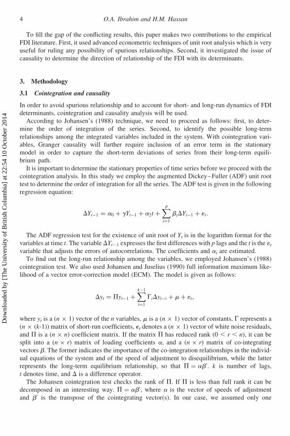
It is important to determine the stationary properties of time series before we proceed with the

cointegration analysis. In this study we employ the augmented Dickey–Fuller (ADF) unit root

test to determine the order of integration for all the series. The ADF test is given in the following

regression equation:

DYt−1 = a0 + gYt−1 + a2t +∑r

i=1

biDYt−1 + 1t.

The ADF regression test for the existence of unit root of Yt is in the logarithm format for the

variables at time t. The variable DYt21 expresses the first differences with p lags and the t is the 1t

variable that adjusts the errors of autocorrelations. The coefficients and ai are estimated.

To find out the long-run relationship among the variables, we employed Johansen’s (1988)

cointegration test. We also used Johansen and Juselius (1990) full information maximum like-

lihood of a vector error-correction model (ECM). The model is given as follows:

Dyt = Pyt−1 +∑k−1

i=1

GiDyt−i + m+ 1t,

where yt is a (n × 1) vector of the n variables, m is a (n × 1) vector of constants, G represents a

(n × (k-1)) matrix of short-run coefficients, e t denotes a (n × 1) vector of white noise residuals,

and P is a (n × n) coefficient matrix. If the matrix P has reduced rank (0 , r , n), it can be

split into a (n × r) matrix of loading coefficients a, and a (n × r) matrix of co-integrating

vectors b. The former indicates the importance of the co-integration relationships in the individ-

ual equations of the system and of the speed of adjustment to disequilibrium, while the latter

represents the long-term equilibrium relationship, so that P = ab′. k is number of lags,

t denotes time, and D is a difference operator.

The Johansen cointegration test checks the rank of P. If P is less than full rank it can be

decomposed in an interesting way. P = ab′, where a is the vector of speeds of adjustment

and b′ is the transpose of the cointegrating vector(s). In our case, we assumed only one

O.A. Ibrahim and H.M. Hassan4

Dow

nloa

ded

by [

The

Uni

vers

ity o

f B

ritis

h C

olum

bia]

at 2

2:54

10

Oct

ober

201

4

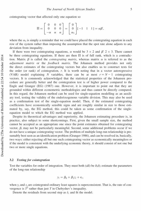
cointegrating vector that affected only one equation so

P =0 0 0

0 0 0

−a a a

⎡⎣

⎤⎦ =

0

0

a3

⎡⎣

⎤⎦[−1 1 1 ] = ab′,

where the a3 is simply a reminder that we could have placed the cointegrating equation in each

row of the system rather than imposing the assumption that the spot rate alone adjusts to any

deviation from inequality.

If there were two cointegrating equations, a would be 3 × 2 and b′ 2 × 3. There cannot

be three cointegrating equations. If there are then P is of full rank, which is a contradic-

tion. Matrix b is called the cointegrating matrix, whereas matrix a is referred to as the

adjustment matrix or the feedback matrix. The Johansen method provides not only

the direct estimates of the cointegrating vectors but also enables us to construct tests for

the order (or rank) of cointegration, r. It is worth noting that in a vector autoregressive

(VAR) model explaining N variables, there can be at most r ¼ N 2 1 cointegrating

vectors. It is commonly acknowledged that the statistical properties of the Johansen pro-

cedure are generally better and the cointegration test is of higher power compared to the

Engle and Granger (EG) (1987) one. However, it is important to point out that they are

grounded within different econometric methodologies and thus cannot be directly compared.

In this regard, the Johansen method can be used for single-equation modelling as an auxili-

ary tool, testing the validity of the endo/exogenous variable division. This may also be used

as a confirmation test of the single-equation model. Then, if the estimated cointegrating

coefficients have economically sensible signs and are roughly similar in size to those esti-

mated by, say, the EG method, this could be taken as some confirmation of the single-

equation model to which the EG method was applied.

Despite its theoretical advantages and superiority, the Johansen estimating procedure is, in

practice, also subject to some shortcomings. First, given the small sample size, the method

cannot be accepted as an appropriate one since the point estimates obtained for cointegrating

vector, b, may not be particularly meaningful. Second, some additional problems occur if we

do not have a unique cointegrating vector. The problem of multiple long-run relationship is pre-

sumably best seen as an identification problem (Granger 1986), and can be resolved in, basically,

two ways: either rejecting all but one such cointegrating vector as economically meaningless or

if the model is consistent with the underlying economic theory, it should consist of not one but

two or more single equations.

3.2 Testing for cointegration

Test the variables for order of integration. They must both (all) be I(d); estimate the parameters

of the long-run relationship

yt = b0 + b1zt + 1t,

when yt and zt are cointegrated ordinary least squares is superconsistent. That is, the rate of con-

vergence is T2 rather than just T in Chebyshev’s inequality.

Denote the residuals from second step as et and fit the model.

The Journal of North African Studies 5

Dow

nloa

ded

by [

The

Uni

vers

ity o

f B

ritis

h C

olum

bia]

at 2

2:54

10

Oct

ober

201

4

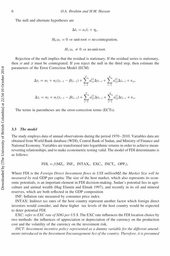
The null and alternate hypotheses are

Det = a1et + ht,

H0:a1 = 0 ⇒ unit root = no cointegration,

H1:a1 = 0 ⇒ no unit root.

Rejection of the null implies that the residual is stationary. If the residual series is stationary,

then yt and zt must be cointegrated. If you reject the null in the third step, then estimate the

parameters of the Error Correction Model (ECM)

Dyt = a1 + ay(yt−1 − bzt−1) +∑p

i−1

a(i)11Dyt−i +

∑q

i−1

a(i)12Dzt−i + 1yt,

Dzt = a2 + az(yt−1 − bzt−1) +∑p

i−1

a(i)21Dyt−i +

∑q

i−1

a(i)22Dzt−i + 1zt.

The terms in parentheses are the error-correction terms (ECTs).

3.3 The model

The study employs data of annual observations during the period 1970–2010. Variables data are

obtained from World Bank database (WDI), Central Bank of Sudan, and Ministry of Finance and

National Economy. Variables are transformed into logarithmic returns in order to achieve mean-

reverting relationships, and to make econometric testing valid. The model of FDI determinants is

as follows:

FDIt = f (MZt, INFt, INTAXt, EXCt, INCTt, OPPt),

Where FDI is the Foreign Direct Investment flows in US$ millionMZ the Market Size will be

measured by real GDP per capita: The size of the host market, which also represents its econ-

omic potentials, is an important element in FDI decision-making. Sudan’s potential lies in agri-

culture and animal wealth (Hag Elamin and Elmak 1997), and recently in its oil and mineral

reserves, which are both reflected in the GDP composition

INF: Inflation rate measured by consumer price index.

INTAX: Indirect tax rates of the host country represent another factor which foreign direct

investors would consider, and these higher tax levels of the host country would be expected

to deter potential FDI.

EXC: refer to EXC rate of SDG per US $. The EXC rate influences the FDI location choice by

two methods: the influences of appreciation or depreciation of the currency on the production

cost and the volatility of the currency on the investment risk.

INCT: Investment incentive policy represented as a dummy variable for the different amend-

ments introduced in the Investment Encouragement Act of the country. Therefore, it is presumed

O.A. Ibrahim and H.M. Hassan6

Dow

nloa

ded

by [

The

Uni

vers

ity o

f B

ritis

h C

olum

bia]

at 2

2:54

10

Oct

ober

201

4

that any amendments are a step forward to overcome the drawbacks in the previous Act. For

more details refer to http://www.sudaninvest.org/English/Default.htm

OPP: It is a standard hypothesis that openness promotes FDI.

Applying logs on both sides of Equation (1) (for ease of interpretation) and denoting the lower

case variables as the natural log of the respective uppercase variable and t for time result in the

econometric version, we obtain

fdit = a+ b1mzt + b2 inft+b3 intaxt +t +b4 exct + b5 inctt + b6 oppt + 1t.

4. Empirical results and discussion

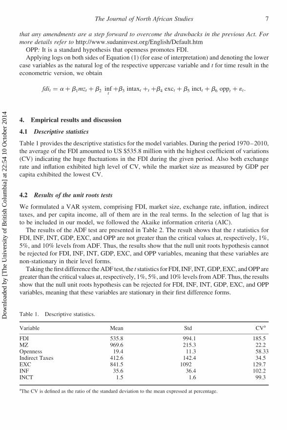
4.1 Descriptive statistics

Table 1 provides the descriptive statistics for the model variables. During the period 1970–2010,

the average of the FDI amounted to US $535.8 million with the highest coefficient of variations

(CV) indicating the huge fluctuations in the FDI during the given period. Also both exchange

rate and inflation exhibited high level of CV, while the market size as measured by GDP per

capita exhibited the lowest CV.

4.2 Results of the unit roots tests

We formulated a VAR system, comprising FDI, market size, exchange rate, inflation, indirect

taxes, and per capita income, all of them are in the real terms. In the selection of lag that is

to be included in our model, we followed the Akaike information criteria (AIC).

The results of the ADF test are presented in Table 2. The result shows that the t statistics for

FDI, INF, INT, GDP, EXC, and OPP are not greater than the critical values at, respectively, 1%,

5%, and 10% levels from ADF. Thus, the results show that the null unit roots hypothesis cannot

be rejected for FDI, INF, INT, GDP, EXC, and OPP variables, meaning that these variables are

non-stationary in their level forms.

Taking the first difference the ADF test, the t statistics for FDI, INF, INT, GDP, EXC, and OPP are

greater than the critical values at, respectively, 1%, 5%, and 10% levels from ADF. Thus, the results

show that the null unit roots hypothesis can be rejected for FDI, INF, INT, GDP, EXC, and OPP

variables, meaning that these variables are stationary in their first difference forms.

Table 1. Descriptive statistics.

Variable Mean Std CVa

FDI 535.8 994.1 185.5MZ 969.6 215.3 22.2Openness 19.4 11.3 58.33Indirect Taxes 412.6 142.4 34.5EXC 841.5 1092 129.7INF 35.6 36.4 102.2INCT 1.5 1.6 99.3

aThe CV is defined as the ratio of the standard deviation to the mean expressed at percentage.

The Journal of North African Studies 7

Dow

nloa

ded

by [

The

Uni

vers

ity o

f B

ritis

h C

olum

bia]

at 2

2:54

10

Oct

ober

201

4

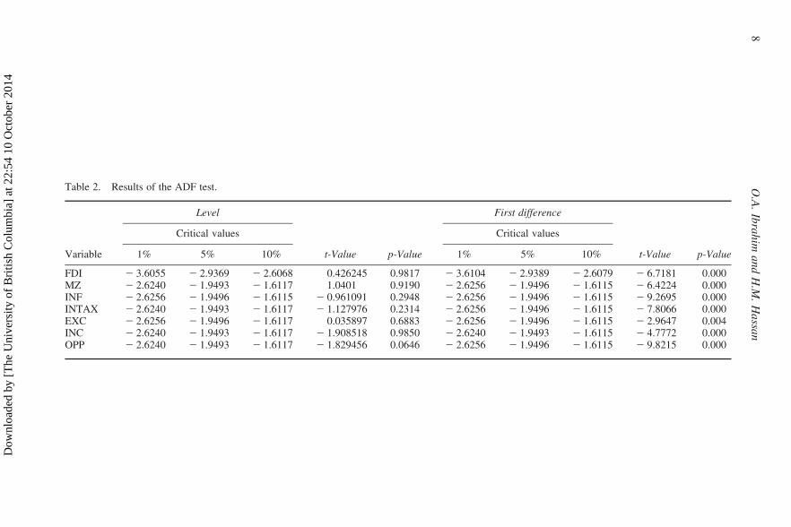
Table 2. Results of the ADF test.

Variable

Level

t-Value p-Value

First difference

t-Value p-Value

Critical values Critical values

1% 5% 10% 1% 5% 10%

FDI 2 3.6055 2 2.9369 2 2.6068 0.426245 0.9817 2 3.6104 2 2.9389 2 2.6079 2 6.7181 0.000MZ 2 2.6240 2 1.9493 2 1.6117 1.0401 0.9190 2 2.6256 2 1.9496 2 1.6115 2 6.4224 0.000INF 2 2.6256 2 1.9496 2 1.6115 2 0.961091 0.2948 2 2.6256 2 1.9496 2 1.6115 2 9.2695 0.000INTAX 2 2.6240 2 1.9493 2 1.6117 2 1.127976 0.2314 2 2.6256 2 1.9496 2 1.6115 2 7.8066 0.000EXC 2 2.6256 2 1.9496 2 1.6117 0.035897 0.6883 2 2.6256 2 1.9496 2 1.6115 2 2.9647 0.004INC 2 2.6240 2 1.9493 2 1.6117 2 1.908518 0.9850 2 2.6240 2 1.9493 2 1.6115 2 4.7772 0.000OPP 2 2.6240 2 1.9493 2 1.6117 2 1.829456 0.0646 2 2.6256 2 1.9496 2 1.6115 2 9.8215 0.000

O.A

.Ib

rah

ima

nd

H.M

.H

assa

n8

Dow

nloa

ded

by [

The

Uni

vers

ity o

f B

ritis

h C

olum

bia]

at 2

2:54

10

Oct

ober

201

4

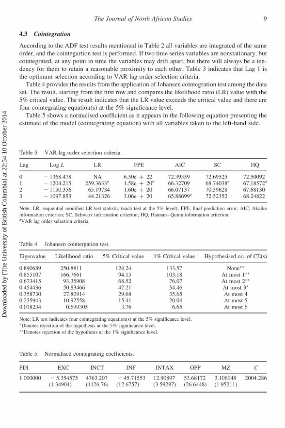
4.3 Cointegration

According to the ADF test results mentioned in Table 2 all variables are integrated of the same

order, and the cointegartion test is performed. If two time series variables are nonstationary, but

cointegrated, at any point in time the variables may drift apart, but there will always be a ten-

dency for them to retain a reasonable proximity to each other. Table 3 indicates that Lag 1 is

the optimum selection according to VAR lag order selection criteria.

Table 4 provides the results from the application of Johansen cointegration test among the data

set. The result, starting from the first row and compares the likelihood ratio (LR) value with the

5% critical value. The result indicates that the LR value exceeds the critical value and there are

four cointegrating equation(s) at the 5% significance level.

Table 5 shows a normalised coefficient as it appears in the following equation presenting the

estimate of the model (cointegrating equation) with all variables taken to the left-hand side.

Table 3. VAR lag order selection criteria.

Lag Log L LR FPE AIC SC HQ

0 2 1368.478 NA 6.50e + 22 72.39359 72.69525 72.500921 2 1204.215 259.3633a 1.58e + 20a 66.32709 68.74038a 67.18572a

2 2 1150.356 65.19734 1.60e + 20 66.07137 70.59628 67.681303 2 1097.853 44.21326 3.06e + 20 65.88699a 72.52352 68.24822

Note: LR, sequential modified LR test statistic (each test at the 5% level); FPE, final prediction error; AIC, Akaike

information criterion; SC, Schwarz information criterion; HQ, Hannan–Quinn information criterion.aVAR lag order selection criteria.

Table 4. Johansen cointergation test.

Eigenvalue Likelihood ratio 5% Critical value 1% Critical value Hypothesised no. of CE(s)

0.890689 250.8811 124.24 133.57 None∗∗

0.855107 166.7661 94.15 103.18 At most 1∗∗

0.673415 93.35908 68.52 76.07 At most 2∗∗

0.454436 50.83466 47.21 54.46 At most 3∗

0.358730 27.80914 29.68 35.65 At most 40.235943 10.92558 15.41 20.04 At most 50.018234 0.699305 3.76 6.65 At most 6

Note: LR test indicates four cointegrating equation(s) at the 5% significance level.∗Denotes rejection of the hypothesis at the 5% significance level.∗∗Denotes rejection of the hypothesis at the 1% significance level.

Table 5. Normalised cointegrating coefficients.

FDI EXC INCT INF INTAX OPP MZ C

1.000000 2 5.354575 4763.207 2 45.71553 12.90897 53.68172 3.106048 2004.286(1.34904) (1126.76) (12.6757) (3.59287) (26.6448) (1.95211)

The Journal of North African Studies 9

Dow

nloa

ded

by [

The

Uni

vers

ity o

f B

ritis

h C

olum

bia]

at 2

2:54

10

Oct

ober

201

4

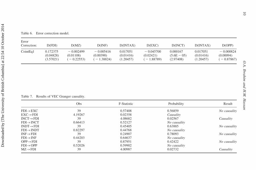
Table 6. Error correction model.

ErrorCorrection: D(FDI) D(MZ) D(INF) D(INTAX) D(EXC) D(INCT) D(INTAX) D(OPP)

CointEq1 0.172375 2 0.002499 2 0.005416 0.017051 2 0.045700 0.000167 0.017051 2 0.000824(0.04828) (0.01108) (0.00390) (0.01416) (0.02421) (5.6E 2 05) (0.01416) (0.00094)(3.57021) ( 2 0.22553) ( 2 1.38824) (1.20457) ( 2 1.88789) (2.97408) (1.20457) ( 2 0.87867)

Table 7. Results of VEC Granger causality.

Obs F-Statistic Probability Result

FDI�EXC 39 0.57408 0.56859 No causalityEXC�FDI 4.19267 0.02358 CausalityINCT�FDI 39 4.08682 0.02567 CausalityFDI�INCT 0.66413 0.52127 No causalityINDT�FDI 39 0.45405 0.63885 No causalityFDI�INDT 0.82297 0.44768 No causalityINF�FDI 39 0.24907 0.78093 No causalityFDI�INF 0.44203 0.64637 No causalityOPP�FDI 39 0.87951 0.42422 No causalityFDI�OPP 0.52026 0.59902 No causalityMZ�FDI 39 4.00987 0.02732 Causality

O.A

.Ib

rah

ima

nd

H.M

.H

assa

n1

0

Dow

nloa

ded

by [

The

Uni

vers

ity o

f B

ritis

h C

olum

bia]

at 2

2:54

10

Oct

ober

201

4

4.4 Error-correction mechanism method with short-run dynamics

Table 6 shows that ECT in all the equations has the negative and positive sign. However, the

ECT in the FDI equation is found statistically significant at the 5% and 1% level. This

implies that FDI is a function of disequilibrium in the cointegrating relationship. The ECT coef-

ficient of 0.1723 for FDI indicates that adjustment towards the equilibrium takes place by

17.23% per annum. On the other hand, the ECT for EXC, INF, OPP and GDP shows a non-sig-

nificant result.

4.5 Granger causality

After determining that the FDI, INF, INCT, MZ, EXC are cointegarted, we proceed wiht the

Grangar causality analysis in order to examine the casual links between the variables under con-

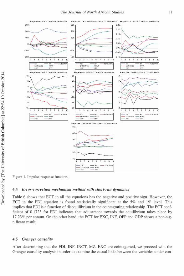
Figure 1. Impulse response function.

The Journal of North African Studies 11

Dow

nloa

ded

by [

The

Uni

vers

ity o

f B

ritis

h C

olum

bia]

at 2

2:54

10

Oct

ober

201

4

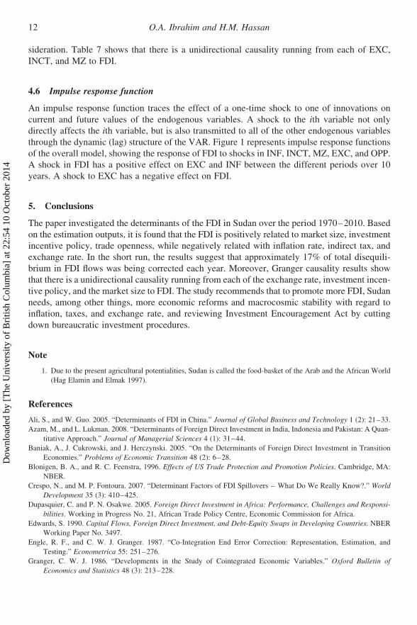
sideration. Table 7 shows that there is a unidirectional causality running from each of EXC,

INCT, and MZ to FDI.

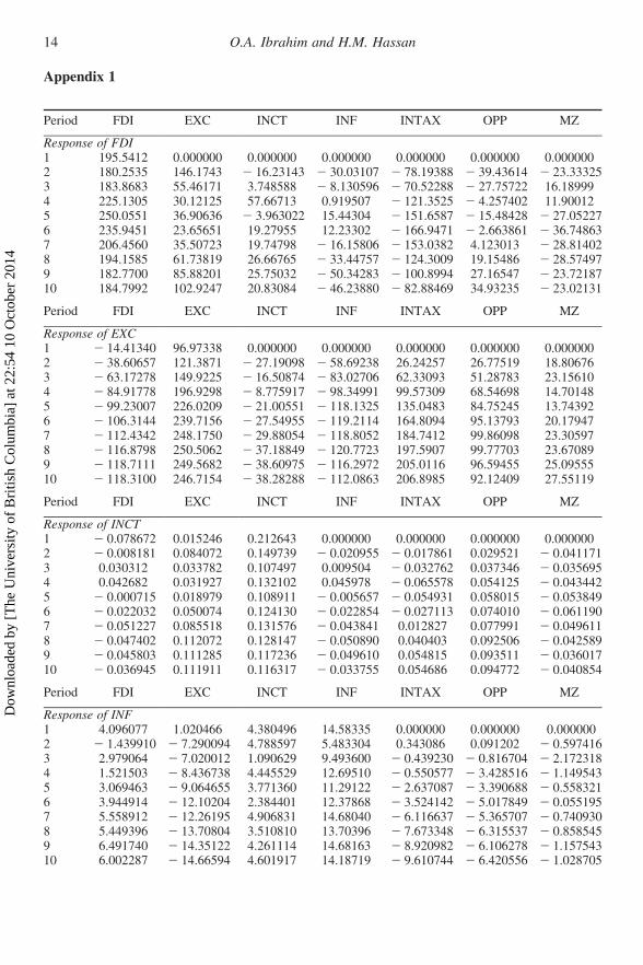
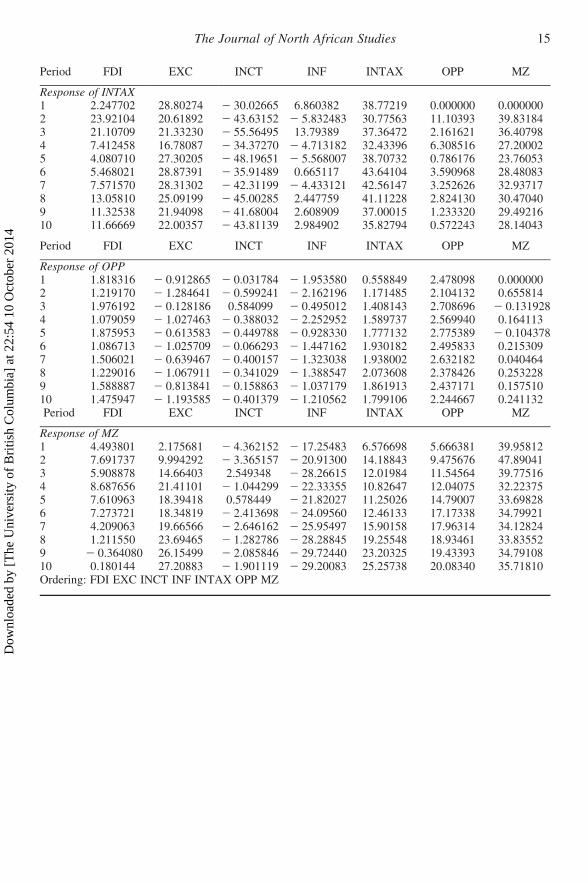
4.6 Impulse response function

An impulse response function traces the effect of a one-time shock to one of innovations on

current and future values of the endogenous variables. A shock to the ith variable not only

directly affects the ith variable, but is also transmitted to all of the other endogenous variables

through the dynamic (lag) structure of the VAR. Figure 1 represents impulse response functions

of the overall model, showing the response of FDI to shocks in INF, INCT, MZ, EXC, and OPP.

A shock in FDI has a positive effect on EXC and INF between the different periods over 10

years. A shock to EXC has a negative effect on FDI.

5. Conclusions

The paper investigated the determinants of the FDI in Sudan over the period 1970–2010. Based

on the estimation outputs, it is found that the FDI is positively related to market size, investment

incentive policy, trade openness, while negatively related with inflation rate, indirect tax, and

exchange rate. In the short run, the results suggest that approximately 17% of total disequili-

brium in FDI flows was being corrected each year. Moreover, Granger causality results show

that there is a unidirectional causality running from each of the exchange rate, investment incen-

tive policy, and the market size to FDI. The study recommends that to promote more FDI, Sudan

needs, among other things, more economic reforms and macrocosmic stability with regard to

inflation, taxes, and exchange rate, and reviewing Investment Encouragement Act by cutting

down bureaucratic investment procedures.

Note

1. Due to the present agricultural potentialities, Sudan is called the food-basket of the Arab and the African World

(Hag Elamin and Elmak 1997).

References

Ali, S., and W. Guo. 2005. “Determinants of FDI in China.” Journal of Global Business and Technology 1 (2): 21–33.

Azam, M., and L. Lukman. 2008. “Determinants of Foreign Direct Investment in India, Indonesia and Pakistan: A Quan-

titative Approach.” Journal of Managerial Sciences 4 (1): 31–44.

Baniak, A., J. Cukrowski, and J. Herczynski. 2005. “On the Determinants of Foreign Direct Investment in Transition

Economies.” Problems of Economic Transition 48 (2): 6–28.

Blonigen, B. A., and R. C. Feenstra, 1996. Effects of US Trade Protection and Promotion Policies. Cambridge, MA:

NBER.

Crespo, N., and M. P. Fontoura. 2007. “Determinant Factors of FDI Spillovers – What Do We Really Know?.” World

Development 35 (3): 410–425.

Dupasquier, C. and P. N. Osakwe. 2005. Foreign Direct Investment in Africa: Performance, Challenges and Responsi-

bilities. Working in Progress No. 21, African Trade Policy Centre, Economic Commission for Africa.

Edwards, S. 1990. Capital Flows, Foreign Direct Investment, and Debt-Equity Swaps in Developing Countries. NBER

Working Paper No. 3497.

Engle, R. F., and C. W. J. Granger. 1987. “Co-Integration End Error Correction: Representation, Estimation, and

Testing.” Econometrica 55: 251–276.

Granger, C. W. J. 1986. “Developments in the Study of Cointegrated Economic Variables.” Oxford Bulletin of

Economics and Statistics 48 (3): 213–228.

O.A. Ibrahim and H.M. Hassan12

Dow

nloa

ded

by [

The

Uni

vers

ity o

f B

ritis

h C

olum

bia]

at 2

2:54

10

Oct

ober

201

4

Hag Elamin, N. A., and E. M. Elmak. 1997. Adjustment Programs and Agricultural Incentives: A Comparative Study.

AERC Research Paper no. 63, Nairobi.

Hasan, Z. 2007. Determinants of Foreign Direct Investment to Developing Countries: Evidence From Malaysia. MPRA,

Paper No. 2822. Accessed December 25, 2011. http//mpra.ub.uni-muenchen.de/2822/

Jaspersen, F., A. Aylward, and A. Knox. 2000. “The Effects of Risk on Private Investment: Africa Compared with Other

Developing Areas.” In Investment and Risk in Africa, edited by P. Collier and C. Pattillo, 71–95. New York:

St Martin’s Press.

Johansen, S. 1988. “Statistical Analysis of Cointegrating Vectors.” Journal of Economic Dynamics and Control 12

(2–3): 231–254.

Johansen, S., and K. Juselius. 1990. “Maximum Likelihood Estimation and Inference on Cointegration – with

Applications to the Demand for Money.” Oxford Bulletin of Economics and Statistics 52 (2): 169–210.

Khondoker, A. M., and K. Kalirajan. 2010. Determinants of Foreign Direct Investment in Developing Countries: A

Comparative Analysis. ASARC WP 2010/13. Accessed February 10, 2012. http://www.crawford.anu.edu.au/

acde/asarc/pdf/papers/2010/WP2010_13.pdf

Kinda, T. 2010. “Investment Climate and FDI in Developing Countries: Firm Level Evidence.” World Development 38

(4): 498–513.

Kozo, K., and S. Urata. 2004. “Exchange Rate, Exchange Rate Volatility, and Foreign Direct Investment.” The World

Economy 27 (10): 1501–1536.

Liu, X., P. Romily, H. Y. Song, and Y. O. Wei. 1997. “Country Characteristics and Foreign Direct Investment in

China: A Panel Data Analysis.” Weltwirschaftliches Archives 133 (2): 313–329.

Lui, L. G., K. Chow, and U. Li. 2006. Determinants of Foreign Direct Investment in East Asia: Did China Crowd Out

FDI From Her Developing East ASEAN Neighbors? Hong Kong Monetary Authority.

Ministry of Cabinet Affairs. 2010. Impediments of Investment in Sudan’ Consultancy Board. Khartoum – Sudan (in

Arabic).

Mwilima, N. 2003. Foreign Direct Investment in Africa. Africa Labour Research Network. Accessed January 4, 2012.

//www.sarpn.org/documents/d0000883/P994

Naeem, K. I., and M. Azam. 2005. “Determinants of Foreign Direct Investment in Pakistan (1970–2000): An Econo-

metrics Approach.” Sarhad Journal of Agriculture 21 (4): 761–764.

Ok, S. T. 2004. “What Drives Foreign Direct Investment into Emerging Markets? Evidence From Turkey.” Emerging

Markets Finance and Trade 40 (4): 101–114.

Quazi, M. R., and M. Mahmud. 2004. Determinants of Foreign Direct Investment in South Asia. Accessed February 13,

2012. http://cob.pvamu.edu/business/WorkingPapers/FDI-MVEA.pdf

Ricci, L. A. 2006. “Uncertainty, Flexible Exchange Rates, and Agglomeration.” Open Economic Review 172 (2):

197–219.

Romer, P. 1993. “Idea Gaps and Object Gaps in Economic Development.” Journal of Monetary Economics 32 (3):

543–573.

Sader, E. 1993. Privatization and Foreign Investment in Developing World. World Bank Working Paper No. 1202.

Schneider, F., and B. Frey. 1985. “Economic and Political Determinants of Foreign Direct Investment.” World

Development 13 (2): 161–175.

Swain, N. J., and Z. Wang. 1997. “Determinants of Inflow of Foreign Direct Investment in Hungary and China: Time-

Series Approach.” Journal of International Development 9 (5): 695–726.

The Arab Investment and Export Credit Guarantee Corporation (Dhaman) Report. 2010. Shuwaikh, Kuwait.

Tuman, J. P., and C. F. Emmert. 1999. “Explaining Japanese Foreign Direct Investment in Latin America, 1979–1992.”

Social Science Quarterly 80: 539–555.

UNCTAD. 2009. World Investment Report 2009: ‘Transnational Corporations, Agricultural Production and Develop-

ment’. New York: United Nations Centre on Transnational Corporations.

UNCTAD. 2011. World Investment Report 2011: Non-Equity Modes of International Production and Development. New

York: United Nations Centre on Transnational Corporations.

Wei, Y., and X. Liu. 2001. Foreign Direct Investment in China: Determinants and Impact. Cheltenham, UK: Edward

Elgar.

World Bank. 1999. Foreign Direct Investment in Bangladesh: Issues of Long-Run Sustainability. Dhaka, Bangladesh:

World Bank, Bangladesh Country Office.

World Bank, Sudan CMU. 2008. Interim Strategy Note. Washington, DC: World Bank.

Yunshi, M., and Y. Jing. 2005. “Overseas Investment Trends Change with times.” China Daily, 11 October.

Zhang, K. H. 2000. “Why is U.S. Direct Investment in China so Cmall?” Contemporary Economic Policy 18 (1): 82–94.

The Journal of North African Studies 13

Dow

nloa

ded

by [

The

Uni

vers

ity o

f B

ritis

h C

olum

bia]

at 2

2:54

10

Oct

ober

201

4

Appendix 1

Period FDI EXC INCT INF INTAX OPP MZ

Response of FDI1 195.5412 0.000000 0.000000 0.000000 0.000000 0.000000 0.0000002 180.2535 146.1743 2 16.23143 2 30.03107 2 78.19388 2 39.43614 2 23.333253 183.8683 55.46171 3.748588 2 8.130596 2 70.52288 2 27.75722 16.189994 225.1305 30.12125 57.66713 0.919507 2 121.3525 2 4.257402 11.900125 250.0551 36.90636 2 3.963022 15.44304 2 151.6587 2 15.48428 2 27.052276 235.9451 23.65651 19.27955 12.23302 2 166.9471 2 2.663861 2 36.748637 206.4560 35.50723 19.74798 2 16.15806 2 153.0382 4.123013 2 28.814028 194.1585 61.73819 26.66765 2 33.44757 2 124.3009 19.15486 2 28.574979 182.7700 85.88201 25.75032 2 50.34283 2 100.8994 27.16547 2 23.7218710 184.7992 102.9247 20.83084 2 46.23880 2 82.88469 34.93235 2 23.02131

Period FDI EXC INCT INF INTAX OPP MZ

Response of EXC1 2 14.41340 96.97338 0.000000 0.000000 0.000000 0.000000 0.0000002 2 38.60657 121.3871 2 27.19098 2 58.69238 26.24257 26.77519 18.806763 2 63.17278 149.9225 2 16.50874 2 83.02706 62.33093 51.28783 23.156104 2 84.91778 196.9298 2 8.775917 2 98.34991 99.57309 68.54698 14.701485 2 99.23007 226.0209 2 21.00551 2 118.1325 135.0483 84.75245 13.743926 2 106.3144 239.7156 2 27.54955 2 119.2114 164.8094 95.13793 20.179477 2 112.4342 248.1750 2 29.88054 2 118.8052 184.7412 99.86098 23.305978 2 116.8798 250.5062 2 37.18849 2 120.7723 197.5907 99.77703 23.670899 2 118.7111 249.5682 2 38.60975 2 116.2972 205.0116 96.59455 25.0955510 2 118.3100 246.7154 2 38.28288 2 112.0863 206.8985 92.12409 27.55119

Period FDI EXC INCT INF INTAX OPP MZ

Response of INCT1 2 0.078672 0.015246 0.212643 0.000000 0.000000 0.000000 0.0000002 2 0.008181 0.084072 0.149739 2 0.020955 2 0.017861 0.029521 2 0.0411713 0.030312 0.033782 0.107497 0.009504 2 0.032762 0.037346 2 0.0356954 0.042682 0.031927 0.132102 0.045978 2 0.065578 0.054125 2 0.0434425 2 0.000715 0.018979 0.108911 2 0.005657 2 0.054931 0.058015 2 0.0538496 2 0.022032 0.050074 0.124130 2 0.022854 2 0.027113 0.074010 2 0.0611907 2 0.051227 0.085518 0.131576 2 0.043841 0.012827 0.077991 2 0.0496118 2 0.047402 0.112072 0.128147 2 0.050890 0.040403 0.092506 2 0.0425899 2 0.045803 0.111285 0.117236 2 0.049610 0.054815 0.093511 2 0.03601710 2 0.036945 0.111911 0.116317 2 0.033755 0.054686 0.094772 2 0.040854

Period FDI EXC INCT INF INTAX OPP MZ

Response of INF1 4.096077 1.020466 4.380496 14.58335 0.000000 0.000000 0.0000002 2 1.439910 2 7.290094 4.788597 5.483304 0.343086 0.091202 2 0.5974163 2.979064 2 7.020012 1.090629 9.493600 2 0.439230 2 0.816704 2 2.1723184 1.521503 2 8.436738 4.445529 12.69510 2 0.550577 2 3.428516 2 1.1495435 3.069463 2 9.064655 3.771360 11.29122 2 2.637087 2 3.390688 2 0.5583216 3.944914 2 12.10204 2.384401 12.37868 2 3.524142 2 5.017849 2 0.0551957 5.558912 2 12.26195 4.906831 14.68040 2 6.116637 2 5.365707 2 0.7409308 5.449396 2 13.70804 3.510810 13.70396 2 7.673348 2 6.315537 2 0.8585459 6.491740 2 14.35122 4.261114 14.68163 2 8.920982 2 6.106278 2 1.15754310 6.002287 2 14.66594 4.601917 14.18719 2 9.610744 2 6.420556 2 1.028705

O.A. Ibrahim and H.M. Hassan14

Dow

nloa

ded

by [

The

Uni

vers

ity o

f B

ritis

h C

olum

bia]

at 2

2:54

10

Oct

ober

201

4

Period FDI EXC INCT INF INTAX OPP MZ

Response of INTAX1 2.247702 28.80274 2 30.02665 6.860382 38.77219 0.000000 0.0000002 23.92104 20.61892 2 43.63152 2 5.832483 30.77563 11.10393 39.831843 21.10709 21.33230 2 55.56495 13.79389 37.36472 2.161621 36.407984 7.412458 16.78087 2 34.37270 2 4.713182 32.43396 6.308516 27.200025 4.080710 27.30205 2 48.19651 2 5.568007 38.70732 0.786176 23.760536 5.468021 28.87391 2 35.91489 0.665117 43.64104 3.590968 28.480837 7.571570 28.31302 2 42.31199 2 4.433121 42.56147 3.252626 32.937178 13.05810 25.09199 2 45.00285 2.447759 41.11228 2.824130 30.470409 11.32538 21.94098 2 41.68004 2.608909 37.00015 1.233320 29.4921610 11.66669 22.00357 2 43.81139 2.984902 35.82794 0.572243 28.14043

Period FDI EXC INCT INF INTAX OPP MZ

Response of OPP1 1.818316 2 0.912865 2 0.031784 2 1.953580 0.558849 2.478098 0.0000002 1.219170 2 1.284641 2 0.599241 2 2.162196 1.171485 2.104132 0.6558143 1.976192 2 0.128186 0.584099 2 0.495012 1.408143 2.708696 2 0.1319284 1.079059 2 1.027463 2 0.388032 2 2.252952 1.589737 2.569940 0.1641135 1.875953 2 0.613583 2 0.449788 2 0.928330 1.777132 2.775389 2 0.1043786 1.086713 2 1.025709 2 0.066293 2 1.447162 1.930182 2.495833 0.2153097 1.506021 2 0.639467 2 0.400157 2 1.323038 1.938002 2.632182 0.0404648 1.229016 2 1.067911 2 0.341029 2 1.388547 2.073608 2.378426 0.2532289 1.588887 2 0.813841 2 0.158863 2 1.037179 1.861913 2.437171 0.15751010 1.475947 2 1.193585 2 0.401379 2 1.210562 1.799106 2.244667 0.241132Period FDI EXC INCT INF INTAX OPP MZ

Response of MZ1 4.493801 2.175681 2 4.362152 2 17.25483 6.576698 5.666381 39.958122 7.691737 9.994292 2 3.365157 2 20.91300 14.18843 9.475676 47.890413 5.908878 14.66403 2.549348 2 28.26615 12.01984 11.54564 39.775164 8.687656 21.41101 2 1.044299 2 22.33355 10.82647 12.04075 32.223755 7.610963 18.39418 0.578449 2 21.82027 11.25026 14.79007 33.698286 7.273721 18.34819 2 2.413698 2 24.09560 12.46133 17.17338 34.799217 4.209063 19.66566 2 2.646162 2 25.95497 15.90158 17.96314 34.128248 1.211550 23.69465 2 1.282786 2 28.28845 19.25548 18.93461 33.835529 2 0.364080 26.15499 2 2.085846 2 29.72440 23.20325 19.43393 34.7910810 0.180144 27.20883 2 1.901119 2 29.20083 25.25738 20.08340 35.71810Ordering: FDI EXC INCT INF INTAX OPP MZ

The Journal of North African Studies 15

Dow

nloa

ded

by [

The

Uni

vers

ity o

f B

ritis

h C

olum

bia]

at 2

2:54

10

Oct

ober

201

4