Detecting Hidden Messages Using Higher-Order

Statistics and Support Vector Machines

Siwei Lyu and Hany Farid

Dartmouth College, Hanover NH 03755, USA,{lsw,farid}@cs.dartmouth.edu,

www.cs.dartmouth.edu/~{lsw,farid}

Abstract. Techniques for information hiding have become increasinglymore sophisticated and widespread. With high-resolution digital imagesas carriers, detecting hidden messages has become considerably moredifficult. This paper describes an approach to detecting hidden messagesin images that uses a wavelet-like decomposition to build higher-orderstatistical models of natural images. Support vector machines are thenused to discriminate between untouched and adulterated images.

1 Introduction

Information hiding techniques (e.g., steganography and watermarking) have re-cently received quite a bit of attention (see [12, 1, 10, 15] for general reviews).With digital images as carriers, detecting the presence of hidden messages posessignificant challenges. Although the presence of embedded messages is often im-perceptible to the human eye, it may nevertheless disturb the statistics of animage. Previous approaches to detecting such deviations [11, 28, 17] typicallyexamine first-order statistical distributions of intensity or transform coefficients(e.g., discrete cosine transform, DCT). The drawback of this analysis is that sim-ple counter-measures that match first-order statistics are likely to foil detection.In contrast, the approach taken here relies on building higher-order statisti-cal models for natural images [13, 19,29, 14, 21] and looking for deviations fromthese models. We show that, across a large number of natural images, there existstrong higher-order statistical regularities within a wavelet-like decomposition,see also [9]. The embedding of a message significantly alters these statistics andthus becomes detectable. Support vector machines (linear and non-linear) areemployed to detect these statistical deviations.

2 Image Statistics

In: 5th International Workshop on Information Hiding, Noordwijkerhout, The Nether-lands, 2002.

ωx

ωy

Fig. 1. An idealized multi-scale and orientation decomposition of frequency space.Shown, from top to bottom, are levels 0, 1, and 2, and from left to right, are thelowpass, vertical, horizontal, and diagonal subbands.

The decomposition of images using basis functions that are localized in spatialposition, orientation, and scale (e.g., wavelets) has proven extremely useful in arange of applications (e.g., image compression, image coding, noise removal, andtexture synthesis). One reason is that such decompositions exhibit statisticalregularities that can be exploited (e.g., [20,18, 2]). Described below is one suchdecomposition, and a set of statistics collected from this decomposition.

The decomposition employed here is based on separable quadrature mirrorfilters (QMFs) [23, 26, 22]. As illustrated in Fig. 1, this decomposition splits thefrequency space into multiple scales and orientations. This is accomplished byapplying separable lowpass and highpass filters along the image axes generat-ing a vertical, horizontal, diagonal and lowpass subband. Subsequent scales arecreated by recursively filtering the lowpass subband. The vertical, horizontal,and diagonal subbands at scale i = 1, ..., n are denoted as Vi(x, y), Hi(x, y), andDi(x, y), respectively. Shown in Fig. 2 is a three-level decomposition of a “disc”image.

Given this image decomposition, the statistical model is composed of themean, variance, skewness and kurtosis of the subband coefficients at each ori-entation and at scales i = 1, ..., n − 1. These statistics characterize the basiccoefficient distributions. The second set of statistics is based on the errors in anoptimal linear predictor of coefficient magnitude. As described in [2], the sub-band coefficients are correlated to their spatial, orientation and scale neighbors.For purposes of illustration, consider first a vertical band, Vi(x, y), at scale i. A

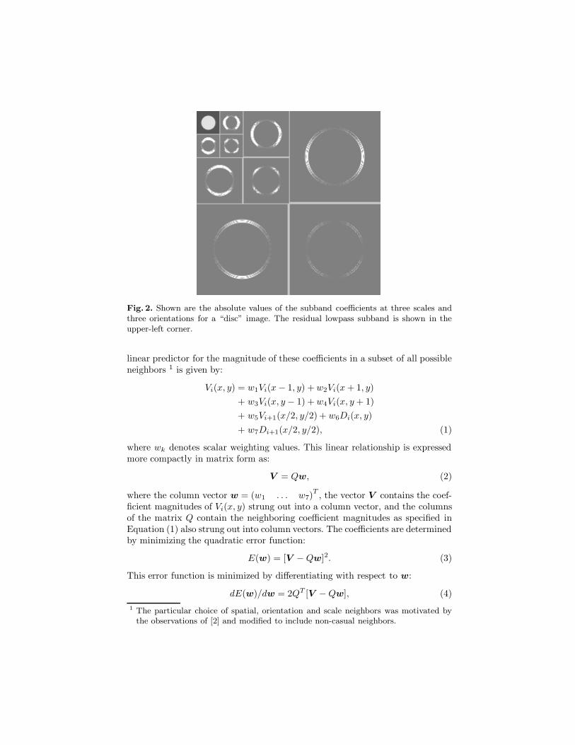
Fig. 2. Shown are the absolute values of the subband coefficients at three scales andthree orientations for a “disc” image. The residual lowpass subband is shown in theupper-left corner.

linear predictor for the magnitude of these coefficients in a subset of all possibleneighbors 1 is given by:

Vi(x, y) = w1Vi(x− 1, y) + w2Vi(x + 1, y)

+ w3Vi(x, y − 1) + w4Vi(x, y + 1)

+ w5Vi+1(x/2, y/2) + w6Di(x, y)

+ w7Di+1(x/2, y/2), (1)

where wk denotes scalar weighting values. This linear relationship is expressedmore compactly in matrix form as:

V = Qw, (2)

where the column vector w = (w1 . . . w7)T, the vector V contains the coef-

ficient magnitudes of Vi(x, y) strung out into a column vector, and the columnsof the matrix Q contain the neighboring coefficient magnitudes as specified inEquation (1) also strung out into column vectors. The coefficients are determinedby minimizing the quadratic error function:

E(w) = [V − Qw]2. (3)

This error function is minimized by differentiating with respect to w:

dE(w)/dw = 2QT [V − Qw], (4)

1 The particular choice of spatial, orientation and scale neighbors was motivated bythe observations of [2] and modified to include non-casual neighbors.

setting the result equal to zero, and solving for w to yield:

w = (QT Q)−1QTV . (5)

The log error in the linear predictor is then given by:

E = log2(V )− log2(|Qw|). (6)

It is from this error that additional statistics are collected, namely the mean,variance, skewness, and kurtosis. This process is repeated for each vertical sub-band at scales i = 1, ..., n− 1, where at each scale a new linear predictor isestimated. A similar process is repeated for the horizontal and diagonal sub-bands. The linear predictor for the horizontal subbands is of the form:

Hi(x, y) = w1Hi(x− 1, y) + w2Hi(x + 1, y)

+ w3Hi(x, y − 1) + w4Hi(x, y + 1)

+ w5Hi+1(x/2, y/2) + w6Di(x, y)

+ w7Di+1(x/2, y/2), (7)

and for the diagonal subbands:

Di(x, y) = w1Di(x− 1, y) + w2Di(x + 1, y)

+ w3Di(x, y − 1) + w4Di(x, y + 1)

+ w5Di+1(x/2, y/2) + w6Hi(x, y)

+ w7Vi(x, y). (8)

The same error metric, Equation (6), and error statistics computed for the verti-cal subbands, are computed for the horizontal and diagonal bands, for a total of12(n−1) error statistics. Combining these statistics with the 12(n−1) coefficientstatistics yields a total of 24(n − 1) statistics that form a feature vector whichis used to discriminate between images that contain hidden messages and thosethat do not.

3 Classification

From the measured statistics of a training set of images with and without hiddenmessages, the goal is to determine whether a test image contains a message. Inearlier work [6], we performed this classification using a Fisher linear discrimi-nant (FLD) analysis [7, 5]. Here a more flexible support vector machine (SVM)classifier is employed [24,25, 3]. We briefly describe, in increasing complexity,three classes of SVMs. The first, linear separable case is mathematically themost straight-forward. The second, linear non-separable case, contends with sit-uations in which a solution cannot be found in the former case, and is mostsimilar to a FLD. The third, non-linear case, affords the most flexible classifi-cation scheme and, in and our application, the best classification accuracy. Forsimplicity a two-class SVM is described throughout.

margin

}

w

b/||w||

(a) (b)

Fig. 3. Linear (a) separable and (b) non-separable support vector machines. Shown isa toy example of a two-class discriminator (white and black dots) for data in R2.

3.1 Linear Separable SVM

Denote the tuple (xi, yi) , i = 1, ..., N as exemplars from a training set of imageswith and without hidden messages. The column vector xi contains the measuredimage statistics as outlined in the previous section, and yi = −1 for images witha hidden message, and yi = 1 for images without a hidden message. The linearseparable SVM classifier amounts to a hyperplane that separates the positiveand negative exemplars, Fig. 3(a). Points which lie on the hyperplane satisfy theconstraint:

wtxi + b = 0, (9)

where w is normal to the hyperplane, |b|/||w|| is the perpendicular distancefrom the origin to the hyperplane, and || · || denotes the Euclidean norm. Definenow the margin for any given hyperplane to be the sum of the distances fromthe hyperplane to the nearest positive and negative exemplar, Fig. 3(a). Theseparating hyperplane is chosen so as to maximize the margin. If a hyperplaneexists that separates all the data then, within a scale factor:

wtxi + b ≥ 1, if yi = 1 (10)

wtxi + b ≤ −1, if yi = −1. (11)

These pair of constraints can be combined into a single set of inequalities:

(wtxi + b) yi − 1 ≥ 0, i = 1, ..., N. (12)

For any given hyperplane that satisfies this constraint, the margin is 2/||w||. Weseek, therefore, to minimize ||w||2 subject to the constraints in Equation (12).

For largely computational reasons, this optimization problem is reformulatedusing Lagrange multipliers, yielding the following Lagrangian:

L(w, b, α1, ..., αN) =1

2||w||2 −

N∑

i=1

αi (wtxi + b) yi +

N∑

i=1

αi, (13)

where αi are the positive Lagrange multipliers. This error function should beminimized with respect to w and b, while requiring that the derivatives of L(·)with respect to each αi is zero and constraining αi ≥ 0, for all i. Because thisis a convex quadratic programming problem, a solution to the dual problemyields the same solution for w, b, and α1, ..., αN. In the dual problem, the sameerror function L(·) is maximized with respect to αi, while requiring that thederivatives of L(·) with respect to w and b are zero and the constraint thatαi ≥ 0. Differentiating with respect to w and b, and setting the results equal tozero yields:

w =

N∑

i=1

αixiyi (14)

N∑

i=1

αiyi = 0. (15)

Substituting these equalities back into Equation (13) yields:

LD =

N∑

i=1

αi −1

2

N∑

i=1

N∑

j=1

αiαjxtixjyiyj. (16)

Maximization of this error function may be realized using any of a number ofgeneral purpose optimization packages that solve linearly constrained convexquadratic problems (see e.g., [8]).

A solution to the linear separable classifier, if it exists, yields values of αi,from which the normal to the hyperplane can be calculated as in Equation (14),and from the Karush-Kuhn-Tucker [8] (KKT) condition:

b =1

N

N∑

i=1

(

yi −wtxi

)

, (17)

for all i, such that αi 6= 0. From the separating hyperplane, w and b, a novelexemplar, z, can be classified by simply determining on which side of the hyper-plane it lies. If the quantity w

tz + b is greater than or equal to zero, then the

exemplar is classified as not having a hidden message, otherwise the exemplar isclassified as containing a hidden message.

3.2 Linear Non-Separable SVM

It is possible, and even likely, that the linear separable SVM will not yield asolution when, for example, the training data do not uniformly lie on eitherside of a separating hyperplane, as illustrated in Fig. 3(b). Such a situationcan be handled by softening the initial constraints of Equation (10) and (11).Specifically, these constraints are modified with “slack” variables, ξi, as follows:

wtxi + b ≥ 1− ξi, if yi = 1 (18)

wtxi + b ≤ −1 + ξi, if yi = −1, (19)

Fig. 4. Non-linear support vector machine, as compared with the linear support vectormachine of Fig. 3.

with ξi ≥ 0, i = 1, ..., N . A training exemplar which lies on the “wrong” side ofthe separating hyperplane will have a value of ξi greater than unity. We seek ahyperplane that minimizes the total training error,

∑

i ξi, while still maximizingthe margin. A simple error function to be minimized is ||w||2/2+C

∑

i ξi, whereC is a user selected scalar value, whose chosen value controls the relative penaltyfor training errors. Minimization of this error is still a quadratic programmingproblem. Following the same procedure as the previous section, the dual problemis expressed as maximizing the error function:

LD =

N∑

i=1

αi −1

2

N∑

i=1

N∑

j=1

αiαjxtixjyiyj, (20)

with the constraint that 0 ≤ αi ≤ C. Note that this is the same error functionas before, Equation (16) with the slightly different constraint that αi is boundedabove by C. Maximization of this error function and computation of the hyper-plane parameters are accomplished as described in the previous section.

3.3 Non-Linear SVM

Fundamental to the SVMs outlined in the previous two sections is the limitationthat the classifier is constrained to a linear hyperplane. Shown in Fig. 4 is anexample of where a non-linear separating surface would greatly improve theclassification accuracy. Non-linear SVMs afford such a classifier by first mappingthe training exemplars into a higher (possibly infinite) dimensional Euclideanspace in which a linear SVM is then employed. Denote this mapping as:

Φ : L → H, (21)

which maps the original training data from L into H. Replacing xi with Φ(xi)everywhere in the training portion of the linear separable or non-separable SVMsof the previous sections yields an SVM in the higher-dimensional space H.

It can, unfortunately, be quite inconvenient to work in the space H as thisspace can be considerably larger than the original L, or even infinite. Note,however, that the error function of Equation (20) to be maximized depends onlyon the inner products of the training exemplars, x

tixj. Given a “kernel” function

such that:

K(xi, xj) = Φ(xi)tΦ(xj), (22)

an explicit computation of Φ can be completely avoided. There are several choicesfor the form of the kernel function, for example, radial basis functions or poly-nomials. Replacing the inner products Φ(xi)

tΦ(xj) with the kernel functionK(xi, xj) yields an SVM in the space H with minimal computational impactover working in the original space L.

With the training stage complete, recall that a novel exemplar, z, is classifiedby determining on which side of the separating hyperplane (specified by w and b)it lies. Specifically, if the quantity w

tΦ(z)+b is greater than or equal to zero, thenthe exemplar is classified as not having a hidden message, otherwise the exemplaris classified as containing a hidden message. The normal to the hyperplane, w,of course now lives in the space H, making this testing impractical. As in thetraining stage, the classification can again be performed via inner products. FromEquation (14):

wtΦ(z) + b =

N∑

i=1

αiΦ(xi)tΦ(z)yi + b

=

N∑

i=1

αiK(xi, z)yi + b. (23)

Thus both the training and classification can be performed in the higher-dimensionalspace, affording a more flexible separating hyperplane and hence better classi-fication accuracy. We next show the performance of a linear non-separable andnon-linear SVM in the detection of hidden messages. The SVMs classify imagesbased on the 72-dimensional feature vector as described in Section 2.

4 Results

Shown in Fig. 5 are several examples taken from a database of natural images 2.These images span decades of digital and traditional photography and consist ofa broad range of intdoor and outdoor scenes. Each 8-bit per channel RGB imageis cropped to a central 640×480 pixel area. Statistics from 1,800 such images arecollected as follows. Each image is first converted from RGB to gray-scale (gray= 0.299R + 0.587G + 0.114B). A four-level, three-orientation QMF pyramid isconstructed for each image, from which a 72-length feature vector of coefficient

2 Images were downloaded from: philip.greenspun.com and reproduced here withpermission from Philip Greeenspun.

Fig. 5. Sample images.

and error statistics is collected, Section 2. To reduce sensitivity to noise in thelinear predictor, only coefficient magnitudes greater than 1.0 are considered.The training set of “no-steg” statistics comes from either 1,800 JPEG images(quality ≈ 75), 1,800 GIF images (LZW compression), or 1,800 TIFF images(no compression). The GIF and TIFF images are converted from their originalJPEG format.

Messages are embedded into JPEG images using either Jsteg3 or OutGuess4

(run with (+) and without (−) statistical correction). Jsteg and OutGuess aretransform-based systems that embed messages by modulating the DCT coef-ficients. Unique to OutGuess is a technique for embedding into only one-halfof the redundant bits and then using the remaining redundant bits to preservethe first-order distribution of DCT coefficients [16]. Messages are embedded intoGIF images using EzStego5 which modulates the least significant bits of thesorted color palette index. Messages are embedded into the TIFF images usinga generic LSB embedding that modulates the least-significant bit of a randomsubset of the pixel intensities. In each case, a message consists of a n× n pixel(n ∈ [32, 256]) central portion of a random image chosen from the same im-age database. After the message is embedded into the cover image, the sametransformation, decomposition, and collection of statistics as described aboveis performed. In all cases the embedded message consists of only the raw pixelintensities (i.e., no image headers).

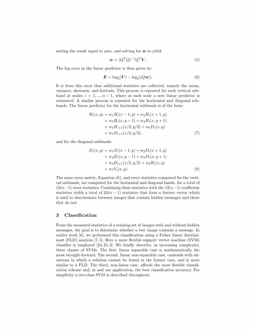
Shown in Fig. 6 is an example cover and message image, and the result ofembedding the message into the cover image. In this example, the mean of theabsolute value of the difference between the cover and steg image is 3.1 intensityvalues with a standard deviation of 3.2. For display purposes the difference imageis renormalized into the range [0, 255].

In the first set of results linear non-separable SVMs, implemented using thefreely available package LIBSVM [4], were separately trained to classify the

3 Jsteg V4, by Derek Upham, is available at ftp.funet.fi4 OutGuess, by Niels Provos, is available at www.outguess.org5 EZStego, by Romana Machado, is available at www.stego.com

cover message steg=cover+message |cover - steg|

Fig. 6. Shown is a cover image and a steg image containing an embedded message.Also shown is the the 256 × 256 message (at scale), and the absolute value of thedifference between the cover and steg image (renormalized into the range [0,255] fordisplay purposes).

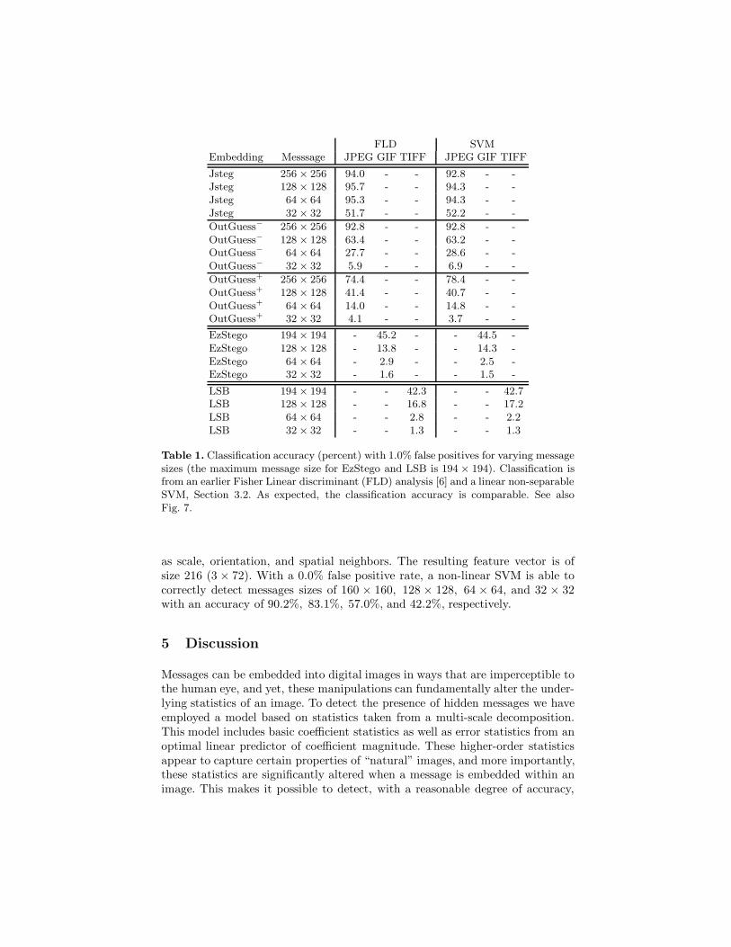
JPEG, GIF and TIFF embeddings. In each case, the training set consists of the1,800 “no-steg” images, and a random subset of 1,800 “steg” images embeddedeither with OutGuess+ , EzStego or LSB, and with varying message sizes. 6 TheSVM parameters were chosen to yield a 1.0% false-positive rate. The trainedSVM is then used to classify all of the remaining previously unseen steg imagesof the same format, Table 1. In this table, the columns correspond to separateclassification results for JPEG, GIF and TIFF format images. Note that theJPEG classifier generalizes to the different embedding programs not previouslyseen by the classifier. Also shown in this table are results from classification em-ploying a Fisher linear discriminant analysis used in our earlier work [6]. Both theFLD and SVM classifiers employ a linear separating hyperplane for classificationso, as expected, performance is similar across these different classifiers.

Shown in Table 2 are classification results for a non-linear SVM (using aradial basis kernel function), also implemented using LIBSVM [4]. In this tableresults are shown for a 1.0% and 0.0% false positive rate. Note the significantimprovement over the linear classifiers of Table 1. Shown in Fig. 7 is a graphicalcomparison of all of these results.

Lastly, we also tested detection accuracy under the F5 embedding algo-rithm [27]. Detection, as described above, was just slightly above chance. Signif-icantly better detection rates were achieved by collecting statistics from withinand across all three color channels (as opposed to analyzing only a grayscaleconverted image). In this case basic coefficient statistics are collected from allthree RGB color channels, and the linear predictor incorporates color as well

6 OutGuess is run with unlimited iterations to find the best embedding. OutGuessimposes limits on the message size, so not all images were able to be used for cover.This is significant only for message sizes of 256×256, where less than 300 steg imageswere generated.

FLD SVMEmbedding Messsage JPEG GIF TIFF JPEG GIF TIFF

Jsteg 256 × 256 94.0 - - 92.8 - -Jsteg 128 × 128 95.7 - - 94.3 - -Jsteg 64 × 64 95.3 - - 94.3 - -Jsteg 32 × 32 51.7 - - 52.2 - -

OutGuess− 256 × 256 92.8 - - 92.8 - -OutGuess− 128 × 128 63.4 - - 63.2 - -OutGuess− 64 × 64 27.7 - - 28.6 - -OutGuess− 32 × 32 5.9 - - 6.9 - -

OutGuess+ 256 × 256 74.4 - - 78.4 - -OutGuess+ 128 × 128 41.4 - - 40.7 - -OutGuess+ 64 × 64 14.0 - - 14.8 - -OutGuess+ 32 × 32 4.1 - - 3.7 - -

EzStego 194 × 194 - 45.2 - - 44.5 -EzStego 128 × 128 - 13.8 - - 14.3 -EzStego 64 × 64 - 2.9 - - 2.5 -EzStego 32 × 32 - 1.6 - - 1.5 -

LSB 194 × 194 - - 42.3 - - 42.7LSB 128 × 128 - - 16.8 - - 17.2LSB 64 × 64 - - 2.8 - - 2.2LSB 32 × 32 - - 1.3 - - 1.3

Table 1. Classification accuracy (percent) with 1.0% false positives for varying messagesizes (the maximum message size for EzStego and LSB is 194 × 194). Classification isfrom an earlier Fisher Linear discriminant (FLD) analysis [6] and a linear non-separableSVM, Section 3.2. As expected, the classification accuracy is comparable. See alsoFig. 7.

as scale, orientation, and spatial neighbors. The resulting feature vector is ofsize 216 (3 × 72). With a 0.0% false positive rate, a non-linear SVM is able tocorrectly detect messages sizes of 160 × 160, 128 × 128, 64 × 64, and 32 × 32with an accuracy of 90.2%, 83.1%, 57.0%, and 42.2%, respectively.

5 Discussion

Messages can be embedded into digital images in ways that are imperceptible tothe human eye, and yet, these manipulations can fundamentally alter the under-lying statistics of an image. To detect the presence of hidden messages we haveemployed a model based on statistics taken from a multi-scale decomposition.This model includes basic coefficient statistics as well as error statistics from anoptimal linear predictor of coefficient magnitude. These higher-order statisticsappear to capture certain properties of “natural” images, and more importantly,these statistics are significantly altered when a message is embedded within animage. This makes it possible to detect, with a reasonable degree of accuracy,

SVM(1.0%) SVM(0.0%)Embedding Messsage JPEG GIF TIFF JPEG GIF TIFF

Jsteg 256 × 256 99.0 - - 98.5 - -Jsteg 128 × 128 99.3 - - 99.0 - -Jsteg 64 × 64 99.1 - - 98.7 - -Jsteg 32 × 32 86.0 - - 74.5 - -

OutGuess− 256 × 256 98.9 - - 97.1 - -OutGuess− 128 × 128 93.8 - - 85.8 - -OutGuess− 64 × 64 72.6 - - 53.1 - -OutGuess− 32 × 32 33.2 - - 14.4 - -

OutGuess+ 256 × 256 95.6 - - 89.5 - -OutGuess+ 128 × 128 82.2 - - 63.7 - -OutGuess+ 64 × 64 54.7 - - 32.1 - -OutGuess+ 32 × 32 21.4 - - 7.2 - -

EzStego 194 × 194 - 77.2 - - 76.9 -EzStego 128 × 128 - 39.2 - - 36.6 -EzStego 64 × 64 - 6.5 - - 4.6 -EzStego 32 × 32 - 2.7 - - 1.5 -

LSB 194 × 194 - - 78.0 - - 77.0LSB 128 × 128 - - 44.7 - - 40.5LSB 64 × 64 - - 6.2 - - 4.2LSB 32 × 32 - - 1.9 - - 1.3

Table 2. Classification accuracy (percent) with 1.0% or 0.0% false positives and forvarying message sizes (the maximum message size for EzStego and LSB is 194× 194).Classification is from a non-linear SVM, Section 3.3. Note the significant improvementin accuracy as compared to a linear classifier, Table 1. See also Fig. 7.

the presence of hidden messages in digital images. This detection is achievedwith either linear or non-linear pattern classification techniques, with the latterproviding significantly better performance. To avoid detection, of course, oneneed only embed a small enough message that does not significantly disturb theimage statistics.

Although not tested here, it is likely that the presence of digital watermarkscould also be detected. Since one of the goals of watermarking is robustness toattack and not necessarily concealment, watermarks typically alter the imagein a more substantial way. As such, it is likely that the underlying statisticswill be more significantly disrupted. Although only tested on images, there isno inherent reason why the approaches described here would not work for audiosignals or video sequences.

The techniques described here would almost certainly benefit from severalextensions: (1) the higher-order statistical model should incorporate correlationswithin and between all three color channels; (2) the classifier should be trainedseparately on different classes of images (e.g., indoor vs. outdoor); and (3) theclassifier should be trained separately on images with varying compression rates.

0

25

50

75

100Jsteg Out− Out+ Ez LSB

256

128

64

32

256

128

64

32

256

128

64

32

194

128

64

32

194

128

64

32 0

25

50

75

100Jsteg Out− Out+ Ez LSB

256

128

64

32

256

128

64

32

256

128

64

32

194

128

64

32

194

128

64

32

(a) (b)

0

25

50

75

100Jsteg Out− Out+ Ez LSB

256

128

64

32

256

128

64

32

256

128

64

32

194

128

64

32

194

128

64

32 0

25

50

75

100Jsteg Out− Out+ Ez LSB

256

128

64

32

256

128

64

32

256

128

64

32

194

128

64

32

194

128

64

32

(c) (d)

Fig. 7. Classification accuracy for (a) Fisher linear discriminant with 1.0% false posi-tives; (b) linear non-separable SVM with 1.0% false positives; (c) non-linear SVM with1.0% false positives; and (d) non-linear SVM with 0.0% false positive rates. The valuesalong the horizontal axis denote the size of the embedded message. See also Tables 1and 2.

One benefit of the higher-order models employed here is that they are notas vulnerable to counter-attacks that match first-order statistical distributionsof pixel intensity or transform coefficients. It is possible, however, that counter-measures will be developed that can foil the detection scheme outlined here. Thedevelopment of such techniques will in turn lead to better detection schemes, andso on.

Acknowledgments

This work is supported by an Alfred P. Sloan Fellowship, a National ScienceFoundation CAREER Award (IIS-99-83806), a Department of Justice Grant(2000-DT-CS-K001), and a departmental National Science Foundation Infras-tructure Grant (EIA-98-02068).

References

1. R.J. Anderson and F.A.P. Petitcolas. On the limits of steganography. IEEE Journal

on Selected Areas in Communications, 16(4):474–481, 1998.2. R.W. Buccigrossi and E.P. Simoncelli. Image compression via joint statistical

characterization in the wavelet domain. IEEE Transactions on Image Processing,8(12):1688–1701, 1999.

3. C.J.C. Burges. A tutorial on support vector machines for pattern recognition. Data

Mining and Knowledge Discovery, 2:121–167, 1998.4. Chih-Chung Chang and Chih-Jen Lin. LIBSVM: a library for support vector ma-

chines, 2001. Software available at http://www.csie.ntu.edu.tw/~cjlin/libsvm.5. R. Duda and P. Hart. Pattern Classification and Scene Analysis. John Wiley and

Sons, 1973.6. H. Farid. Detecting hidden messages using higher-order statistical models. In

International Conference on Image Processing, page (to appear), Rochester, NewYork, 2002.

7. R. Fisher. The use of multiple measures in taxonomic problems. Annals of Eugen-

ics, 7:179–188, 1936.8. R. Fletcher. Practical Methods of Optimization. John Wiley and Sons, 2nd edition,

1987.9. J. Fridrich and M. Goljan. Practical steganalysis: State of the art. In SPIE

Photonics West, Electronic Imaging, San Jose, CA, 2002.10. N. Johnson and S. Jajodia. Exploring steganography: seeing the unseen. IEEE

Computer, pages 26–34, 1998.11. N. Johnson and S. Jajodia. Steganalysis of images created using current steganog-

raphy software. Lecture notes in Computer Science, pages 273–289, 1998.12. D. Kahn. The history of steganography. In Proceedings of Information Hiding,

First International Workshop, Cambridge, UK, 1996.13. D. Kersten. Predictability and redundancy of natural images. Journal of the

Optical Society of America A, 4(12):2395–2400, 1987.14. G. Krieger, C. Zetzsche, and E. Barth. Higher-order statistics of natural images and

their exploitation by operators selective to intrinsic dimensionality. In Proceedings

of the IEEE Signal Processing Workshop on Higher-Order Statistics, pages 147–151, Banff, Alta., Canada, 1997.

15. E.A.P. Petitcolas, R.J. Anderson, and M.G. Kuhn. Information hiding - a survey.Proceedings of the IEEE, 87(7):1062–1078, 1999.

16. N. Provos. Defending against statistical steganalysis. In 10th USENIX Security

Symposium, Washington, DC, 2001.17. N. Provos and P. Honeyman. Detecting steganographic content on the internet.

Technical Report CITI 01-1a, University of Michigan, 2001.18. R. Rinaldo and G. Calvagno. Image coding by block prediction of multiresolution

subimages. IEEE Transactions on Image Processing, 4(7):909–920, 1995.19. D.L. Ruderman and W. Bialek. Statistics of natural image: Scaling in the woods.

Phys. Rev. Letters, 73(6):814–817, 1994.20. J. Shapiro. Embedded image coding using zerotrees of wavelet coefficients. IEEE

Transactions on Signal Processing, 41(12):3445–3462, 1993.21. E.P. Simoncelli. Modeling the joint statistics of images in the wavelet domain. In

Proceedings of the 44th Annual Meeting, volume 3813, Denver, CO, USA, 1999.22. E.P. Simoncelli and E.H. Adelson. Subband image coding, chapter Subband trans-

forms, pages 143–192. Kluwer Academic Publishers, 1990.

23. P.P. Vaidyanathan. Quadrature mirror filter banks, M-band extensions and perfectreconstruction techniques. IEEE ASSP Magazine, pages 4–20, 1987.

24. V. Vapnik. The nature of statistical learning theory. Spring Verlag, 1995.25. V. Vapnik. Statistical learning theory. John Wiley and Sons, 1998.26. M. Vetterli. A theory of multirate filter banks. IEEE Transactions on ASSP,

35(3):356–372, 1987.27. A. Westfeld. High capacity depsite better steganalysis: F5- a steganographic algo-

rithm. In Fourth Information Hiding Workshop, pages 301–315, Pittsburgh, PA,USA, 2001.

28. A. Westfeld and A. Pfitzmann. Attacks on steganographic systems. In Proceedings

of Information Hiding, Third International Workshop, Dresden, Germany, 1999.29. S.C. Zhu, Y. Wu, and D. Mumford. Filters, random fields and maximum entropy

(frame) - towards the unified theory for texture modeling. In IEEE Conference

Computer Vision and Pattern Recognition, pages 686–693, 1996.