Design of an Active 1-DOF Lower-Limb Exoskeleton with Inertia

Compensation

Gabriel Aguirre-Ollinger, J. Edward Colgate, Michael A. Peshkin and Ambarish Goswami

September 2, 2010

Abstract

Limited research has been done on exoskeletons to enable faster movements of the lower extremities.

An exoskeleton’s mechanism can actually hinder agility by adding weight, inertia and friction to the legs;

compensating inertia through control is particularly difficult due to instability issues. The added inertia

will reduce the natural frequency of the legs, probably leading to lower step frequency during walking.

We present a control method that produces an approximate compensation of an exoskeleton’s inertia.

The aim is making the natural frequency of the exoskeleton-assisted leg larger than that of the unaided

leg. The method uses admittance control to compensate the weight and friction of the exoskeleton.

Inertia compensation is emulated by adding a feedback loop consisting of low-pass filtered acceleration

multiplied by a negative gain. This gain simulates negative inertia in the low-frequency range. We tested

the controller on a statically supported, single-DOF exoskeleton that assists swing movements of the leg.

Subjects performed movement sequences, first unassisted and then using the exoskeleton, in the context

of a computer-based task resembling a race. With zero inertia compensation, the steady-state frequency

of leg swing was consistently reduced. Adding inertia compensation enabled subjects to recover their

normal frequency of swing.

Keywords: Exoskeleton, rehabilitation robotics, lower-limb assistance, admittance control

1 Nomenclature

1.1 Symbols Ih, bh, kh = Moment of inertia (kg-m2), damping (N-m-s/rad) and stiffness (N-m/rad) of the humanlimb. Ide , bd

e , kde = Virtual moment of inertia, damping and stiffness of the exoskeleton’s drive mechanism in

the controller’s admittance model. Im = Moment of inertia of the exoskeleton’s servo motor, reflected on the output shaft. bc, kc = Exoskeleton cable drive’s damping and stiffness. Is = Exoskeleton’s output drive inertia (moment of inertia of the mechanical components between thecable and the torque sensor). Iarm, barm, karm = Moment of inertia, damping and stiffness of the exoskeleton’s arm. Ic = Emulated inertia compensator’s gain (kg-m2). ωlo = Cutoff frequency (rad/s) of the inertia compensator’s low-pass filter. ωn,e = Natural frequency of the exoskeleton drive. τh = Net muscle torque (N-m) acting on the human limb’s joint. τm = Torque exerted by the exoskeleton’s actuator.

1

τs = Torque measured by the exoskeleton’s torque sensor. wm = Angular velocity (rad/s) of the servo motor reflected on the output shaft. ws = Angular velocity of the exoskeleton’s drive output shaft. Ωh = RMS angular velocity (rad/s) of swing of the human limb. fc = Frequency of leg swing (Hz). Ac = Amplitude of leg swing (rad). xref = Horizontal position (dimensionless) of the target cursor on the graphic user interface. xh = Horizontal position of the subject’s cursor on the graphic user interface.

1.2 Transfer functions Ye(s) = Two-port admittance of the physical exoskeleton’s drive. Y de (s) = Virtual admittance model followed by the admittance controller. It represents the desired

admittance of the torque sensor port. Y se (s) = Actual closed-loop admittance at the torque sensor port. Y pe (s) = Closed-loop admittance at the exoskeleton’s port of interaction with the user (ankle brace). Y he (s) = Admittance of the human leg when coupled to the exoskeleton (defined as the ratio of ws(s)

to τh(s)). Zarm(s) = Impedance of the exoskeleton’s arm. Zh(s) = Impedance of the human limb.

2 Introduction

In recent years, different types of exoskeletons and orthotic devices have been developed to assist lower-limbmotion. Applications for these devices usually fall into either of two broad categories: (1) augmenting themuscular force of healthy subjects, and (2) rehabilitation of people with motion impairments. Most of the ex-isting implementations in the former group are designed to either enhance the user’s capability to carry heavyloads [Lee and Sankai, 2003, Kawamoto and Sankai, 2005, Kazerooni et al., 2005, Walsh et al., 2006] or re-duce muscle activation during walking [Banala et al., 2006, Sawicki and Ferris, 2009, Lee and Sankai, 2002].Rehabilitation-oriented applications include training devices for gait correction [Jezernik et al., 2004, Banala et al., 2009]and devices that apply controlled forces to the extremities in substitution of a therapist [Veneman et al., 2007].

Although significant advances have been made in the engineering aspects of exoskeleton design (mecha-tronics, computer control, actuators), the physiological aspects of wearing an exoskeleton are less well under-stood. A common observation in recent reviews on exoskeleton research [Ferris et al., 2005, Ferris et al., 2007,Dollar and Herr, 2008] has been the absence of reports of exoskeletons reducing the metabolic cost of walking.Another little-researched topic has been the effect of an exoskeleton on the agility of the user’s movements.At this point we are not aware of any studies addressing how an exoskeleton can affect the user’s selectedspeed of walking, or the ability to accelerate the legs when quick movements are needed.

The present study constitutes a first step towards enabling an exoskeleton to increase the agility of thelower extremities. At preferred walking speeds, the swing leg behaves as a pendulum oscillating close toits natural frequency [Kuo, 2001]. The swing phase of walking takes advantage of this pendular motion inorder to reduce the metabolic cost of walking. Thus we theorize that a wearable exoskeleton could be usedto increase the natural frequency of the legs, and in doing so enable users to walk comfortably at higherspeeds. Although a few studies have been conducted on the modulation of leg swing frequency by means of

2

an exoskeleton [Uemura et al., 2006, Lee and Sankai, 2005], to the best of our knowledge this effect has notyet been linked experimentally to the kinematics and energetics of walking.

The main difficulty in using an exoskeleton to increase the agility of leg movements is that the exoskele-ton’s mechanism adds extra impedance to the legs. Therefore the mechanism by itself can be expected tomake the legs’ movements slower, not faster. And while it is quite feasible to mask the weight and thefriction of the mechanism using control, compensating the mechanism’s inertia is considerably more difficultdue to stability issues [Newman, 1992, Buerger and Hogan, 2007]. All other things being equal, the inertiaadded by the exoskeleton will probably reduce the pendulum frequency of the legs, which can have importantconsequences on the metabolic cost and the speed of walking. A study by Browning [Browning et al., 2007]found that adding masses to the leg increases the metabolic cost of walking. This cost was strongly corre-lated to the moment of inertia of the loaded leg. A similar study by Royer [Royer and Martin, 2005] showedthat loading the legs increases the swing time and the stride time during walking. The findings from bothstudies may be explained by the metabolic cost of swinging the leg. In an experiment reported by Doke[Doke et al., 2005], subjects swung one leg freely at different frequencies with fixed amplitude. It was foundthat the metabolic cost of swinging the leg has a minimum near the natural frequency of the leg, and in-creases with the fourth power of frequency. Thus if the exoskeleton’s inertia reduces the natural frequencyof the leg it is very likely that users will reduce their chosen frequency of leg swing accordingly.

The notion of compensating the inertia of the exoskeleton through control leads to an interesting prospect:to not only compensate the drop in the natural frequency of the legs caused by the exoskeleton’s mechanism,but to actually make the natural frequency of the exoskeleton-assisted leg higher than that of the unaided leg.This in turn raises two possible research questions. First, if the exoskeleton modifies the natural frequencyof the leg, will people modify their frequency of leg swing accordingly? Second, how does the behavior ofmetabolic cost change when the natural frequency is modified, i.e. does the new natural frequency accuratelypredict the minimum metabolic cost?

In this paper we address the first question. We present a control method that produces an approximatecompensation of an exoskeleton’s inertia. We tested our method on a statically mounted, single-DOF ex-oskeleton [Aguirre-Ollinger et al., 2007b, Aguirre-Ollinger et al., 2007a] that assists the user in performingknee flexions and extensions. The exoskeleton has a “baseline” mode of operation in which an admittancecontroller masks the the weight and the dissipative effects (friction, damping) of the exoskeleton’s mecha-nism, thereby making the exoskeleton behave as a pure inertia. An acceleration feedback loop is then addedto compensate the exoskeleton’s inertia at low frequencies. We conducted an experiment in which subjectsperformed multiple series of leg-swing movements in the context of a computer-based pursuit task. Subjectsmoved their leg under three different experimental conditions: (1) leg unaided, (2) wearing the exoskeleton in“baseline” state and (3) wearing the exoskeleton with inertia compensation on. The effects of the exoskeletonon the frequency of leg swing are analyzed and discussed.

3 Exoskeleton design and construction

We designed and built a stationary 1-DOF exoskeleton for assisting knee flexion and extension exercises(Figure 1). Our aim was to use the pendular motion of the leg’s shank as a scaled-down model of the swingmotion of the entire leg when walking, and to investigate the effects of an active exoskeleton dynamics onthe kinematics and energetics of leg-swing motion.

In order to specify the torque requirements for our 1-DOF exoskeleton, we surveyed reported values ofknee torque during normal walking. Kerrigan [Kerrigan et al., 2000] reported an extensive study on the kneejoint torques of barefoot walking. The peak knee torques reported there were 0.34±0.15 N-m/kg-m for womenand 0.32±0.15 N-m/kg-m for men. Thus for a male subject with body mass of 80 kg and height of 1.80 m, thepeak knee torque during normal walking should be about 45 N-m. DeVita [DeVita and Hortobagyi, 2003]reported peak knee torques ranging from 0.39 N-m/kg for obese subjects to 0.97 N-m/kg for lean subjects.From these data, we concluded that an actuator-transmission combination capable of delivering about 20N-m of continuous torque would be sufficient to produce significantly large assistive torques.

Figure 2 shows a CAD model of the exoskeleton’s main assembly, consisting of a servo motor, a cable-drivetransmission and a pivoting arm. The motor is a Kollmorgen (Radford, VA, USA) brushless direct-drive ACmotor with a power rating of 0.99 kW and a continuous torque rating of 2.0 N-m. The motor features a

3

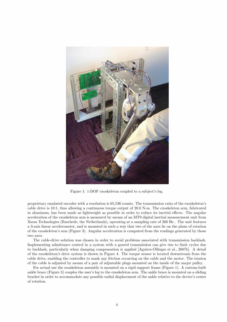
Figure 1: 1-DOF exoskeleton coupled to a subject’s leg.

proprietary emulated encoder with a resolution is 65,536 counts. The transmission ratio of the exoskeleton’scable drive is 10:1, thus allowing a continuous torque output of 20.0 N-m. The exoskeleton arm, fabricatedin aluminum, has been made as lightweight as possible in order to reduce its inertial effects. The angularacceleration of the exoskeleton arm is measured by means of an MT9 digital inertial measurement unit fromXsens Technologies (Enschede, the Netherlands), operating at a sampling rate of 200 Hz . The unit featuresa 3-axis linear accelerometer, and is mounted in such a way that two of the axes lie on the plane of rotationof the exoskeleton’s arm (Figure 3). Angular acceleration is computed from the readings generated by thosetwo axes.

The cable-drive solution was chosen in order to avoid problems associated with transmission backlash.Implementing admittance control in a system with a geared transmission can give rise to limit cycles dueto backlash, particularly when damping compensation is applied [Aguirre-Ollinger et al., 2007b]. A detailof the exoskeleton’s drive system is shown in Figure 4. The torque sensor is located downstream from thecable drive, enabling the controller to mask any friction occurring on the cable and the motor. The tensionof the cable is adjusted by means of a pair of adjustable plugs mounted on the inside of the major pulley.

For actual use the exoskeleton assembly is mounted on a rigid support frame (Figure 1). A custom-builtankle brace (Figure 3) couples the user’s leg to the exoskeleton arm. The ankle brace is mounted on a slidingbracket in order to accommodate any possible radial displacement of the ankle relative to the device’s centerof rotation.

4

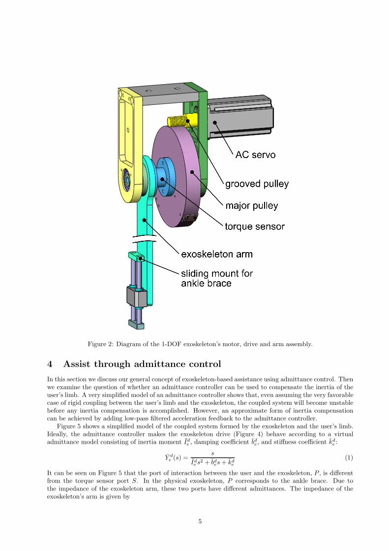
Figure 2: Diagram of the 1-DOF exoskeleton’s motor, drive and arm assembly.

4 Assist through admittance control

In this section we discuss our general concept of exoskeleton-based assistance using admittance control. Thenwe examine the question of whether an admittance controller can be used to compensate the inertia of theuser’s limb. A very simplified model of an admittance controller shows that, even assuming the very favorablecase of rigid coupling between the user’s limb and the exoskeleton, the coupled system will become unstablebefore any inertia compensation is accomplished. However, an approximate form of inertia compensationcan be achieved by adding low-pass filtered acceleration feedback to the admittance controller.

Figure 5 shows a simplified model of the coupled system formed by the exoskeleton and the user’s limb.Ideally, the admittance controller makes the exoskeleton drive (Figure 4) behave according to a virtualadmittance model consisting of inertia moment Id

e , damping coefficient bde, and stiffness coefficient kd

e :

Y de (s) =

s

Ide s2 + bd

es + kde

(1)

It can be seen on Figure 5 that the port of interaction between the user and the exoskeleton, P , is differentfrom the torque sensor port S. In the physical exoskeleton, P corresponds to the ankle brace. Due tothe impedance of the exoskeleton arm, these two ports have different admittances. The impedance of theexoskeleton’s arm is given by

5

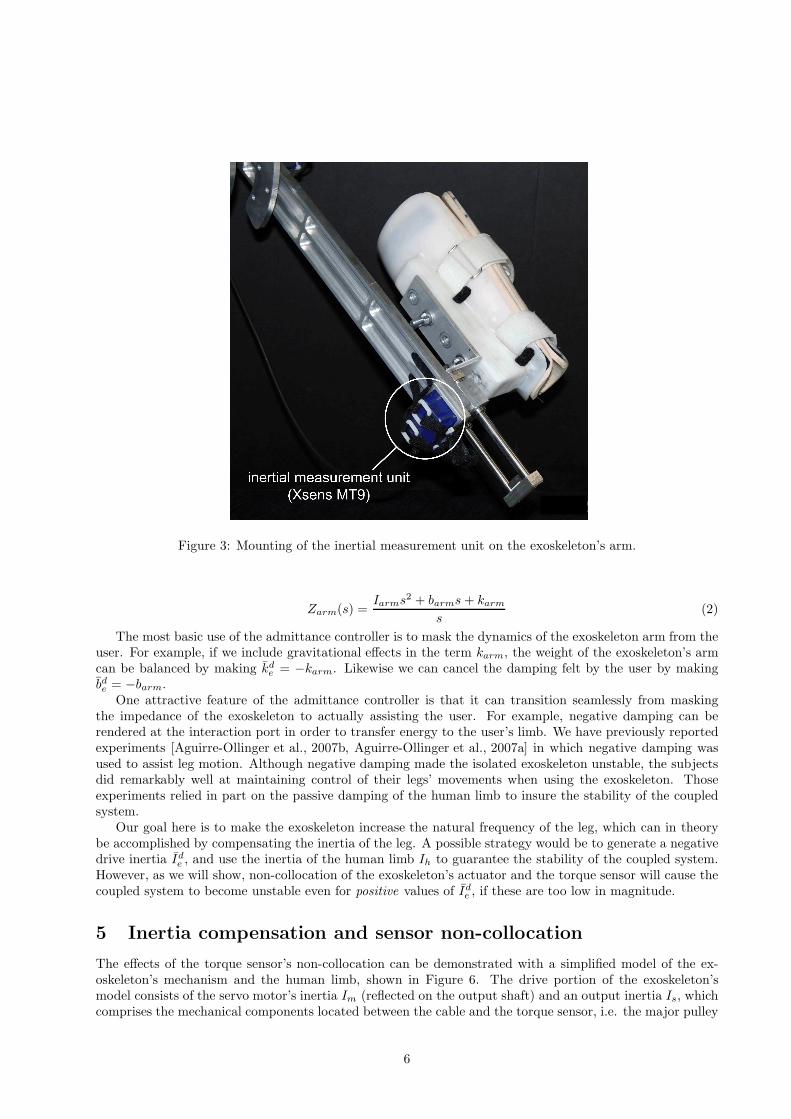
Figure 3: Mounting of the inertial measurement unit on the exoskeleton’s arm.

Zarm(s) =Iarms2 + barms + karm

s(2)

The most basic use of the admittance controller is to mask the dynamics of the exoskeleton arm from theuser. For example, if we include gravitational effects in the term karm, the weight of the exoskeleton’s armcan be balanced by making kd

e = −karm. Likewise we can cancel the damping felt by the user by makingbde = −barm.

One attractive feature of the admittance controller is that it can transition seamlessly from maskingthe impedance of the exoskeleton to actually assisting the user. For example, negative damping can berendered at the interaction port in order to transfer energy to the user’s limb. We have previously reportedexperiments [Aguirre-Ollinger et al., 2007b, Aguirre-Ollinger et al., 2007a] in which negative damping wasused to assist leg motion. Although negative damping made the isolated exoskeleton unstable, the subjectsdid remarkably well at maintaining control of their legs’ movements when using the exoskeleton. Thoseexperiments relied in part on the passive damping of the human limb to insure the stability of the coupledsystem.

Our goal here is to make the exoskeleton increase the natural frequency of the leg, which can in theorybe accomplished by compensating the inertia of the leg. A possible strategy would be to generate a negativedrive inertia Id

e , and use the inertia of the human limb Ih to guarantee the stability of the coupled system.However, as we will show, non-collocation of the exoskeleton’s actuator and the torque sensor will cause thecoupled system to become unstable even for positive values of Id

e , if these are too low in magnitude.

5 Inertia compensation and sensor non-collocation

The effects of the torque sensor’s non-collocation can be demonstrated with a simplified model of the ex-oskeleton’s mechanism and the human limb, shown in Figure 6. The drive portion of the exoskeleton’smodel consists of the servo motor’s inertia Im (reflected on the output shaft) and an output inertia Is, whichcomprises the mechanical components located between the cable and the torque sensor, i.e. the major pulley

6

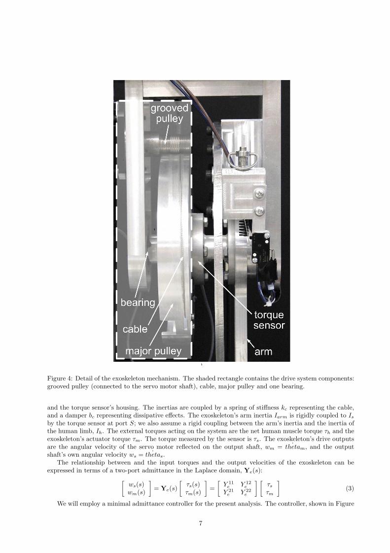
Figure 4: Detail of the exoskeleton mechanism. The shaded rectangle contains the drive system components:grooved pulley (connected to the servo motor shaft), cable, major pulley and one bearing.

and the torque sensor’s housing. The inertias are coupled by a spring of stiffness kc representing the cable,and a damper bc representing dissipative effects. The exoskeleton’s arm inertia Iarm is rigidly coupled to Is

by the torque sensor at port S; we also assume a rigid coupling between the arm’s inertia and the inertia ofthe human limb, Ih. The external torques acting on the system are the net human muscle torque τh and theexoskeleton’s actuator torque τm. The torque measured by the sensor is τs. The exoskeleton’s drive outputsare the angular velocity of the servo motor reflected on the output shaft, wm = ˙thetam, and the outputshaft’s own angular velocity ws = ˙thetas.

The relationship between and the input torques and the output velocities of the exoskeleton can beexpressed in terms of a two-port admittance in the Laplace domain, Ye(s):

[

ws(s)wm(s)

]

= Ye(s)

[

τs(s)τm(s)

]

=

[

Y 11e Y 12

e

Y 21e Y 22

e

] [

τs

τm

]

(3)

We will employ a minimal admittance controller for the present analysis. The controller, shown in Figure

7

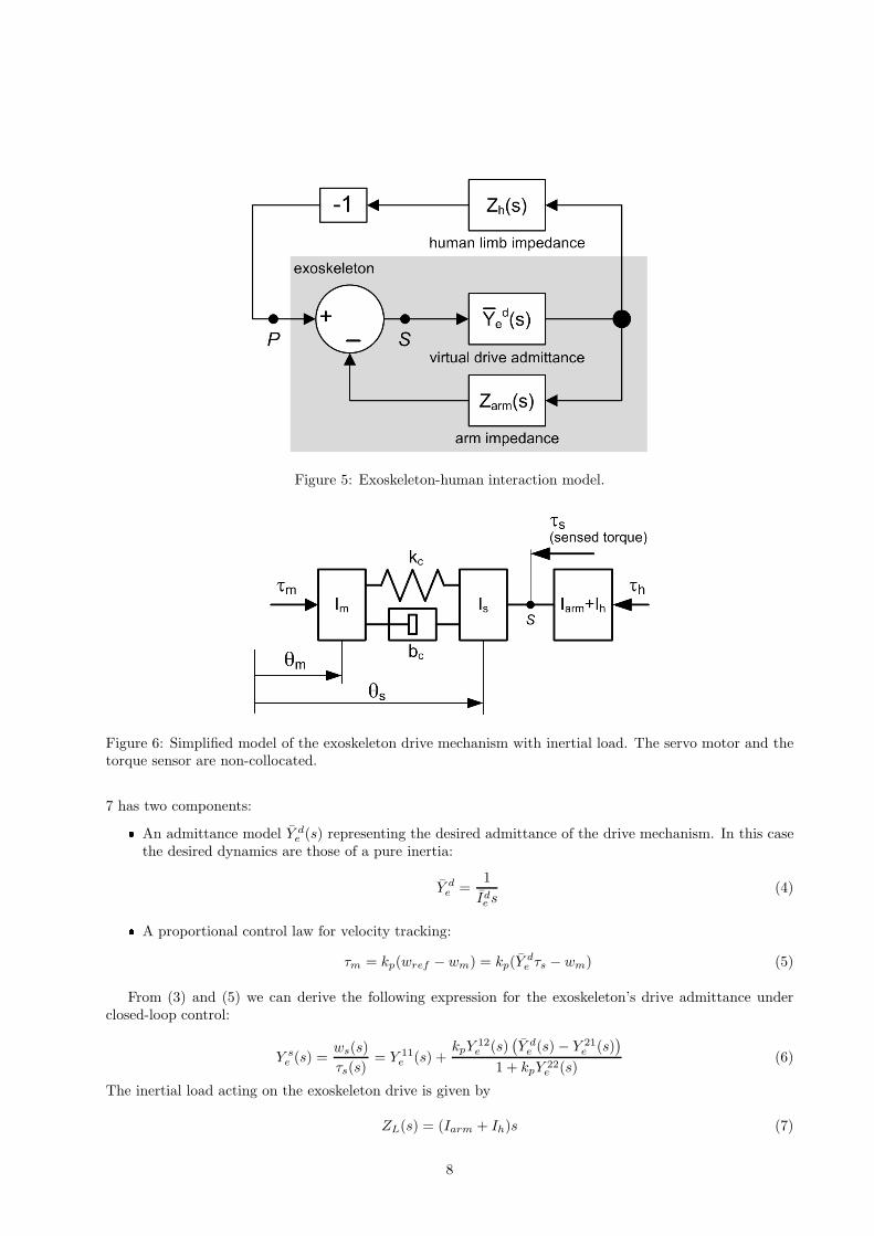
Figure 5: Exoskeleton-human interaction model.

Figure 6: Simplified model of the exoskeleton drive mechanism with inertial load. The servo motor and thetorque sensor are non-collocated.

7 has two components: An admittance model Y de (s) representing the desired admittance of the drive mechanism. In this case

the desired dynamics are those of a pure inertia:

Y de =

1

Ide s

(4) A proportional control law for velocity tracking:

τm = kp(wref − wm) = kp(Yde τs − wm) (5)

From (3) and (5) we can derive the following expression for the exoskeleton’s drive admittance underclosed-loop control:

Y se (s) =

ws(s)

τs(s)= Y 11

e (s) +kpY

12e (s)

(

Y de (s) − Y 21

e (s))

1 + kpY 22e (s)

(6)

The inertial load acting on the exoskeleton drive is given by

ZL(s) = (Iarm + Ih)s (7)

8

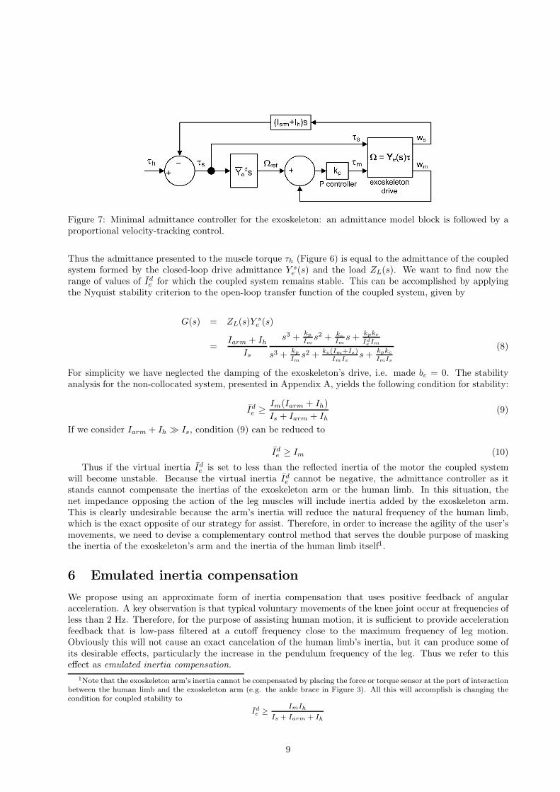
Figure 7: Minimal admittance controller for the exoskeleton: an admittance model block is followed by aproportional velocity-tracking control.

Thus the admittance presented to the muscle torque τh (Figure 6) is equal to the admittance of the coupledsystem formed by the closed-loop drive admittance Y s

e (s) and the load ZL(s). We want to find now therange of values of Id

e for which the coupled system remains stable. This can be accomplished by applyingthe Nyquist stability criterion to the open-loop transfer function of the coupled system, given by

G(s) = ZL(s)Y se (s)

=Iarm + Ih

Is

s3 +kp

Ims2 + kc

Ims +

kpkc

Ide Im

s3 +kp

Ims2 + kc(Im+Is)

ImIss +

kpkc

ImIs

(8)

For simplicity we have neglected the damping of the exoskeleton’s drive, i.e. made bc = 0. The stabilityanalysis for the non-collocated system, presented in Appendix A, yields the following condition for stability:

Ide ≥ Im(Iarm + Ih)

Is + Iarm + Ih

(9)

If we consider Iarm + Ih ≫ Is, condition (9) can be reduced to

Ide ≥ Im (10)

Thus if the virtual inertia Ide is set to less than the reflected inertia of the motor the coupled system

will become unstable. Because the virtual inertia Ide cannot be negative, the admittance controller as it

stands cannot compensate the inertias of the exoskeleton arm or the human limb. In this situation, thenet impedance opposing the action of the leg muscles will include inertia added by the exoskeleton arm.This is clearly undesirable because the arm’s inertia will reduce the natural frequency of the human limb,which is the exact opposite of our strategy for assist. Therefore, in order to increase the agility of the user’smovements, we need to devise a complementary control method that serves the double purpose of maskingthe inertia of the exoskeleton’s arm and the inertia of the human limb itself1.

6 Emulated inertia compensation

We propose using an approximate form of inertia compensation that uses positive feedback of angularacceleration. A key observation is that typical voluntary movements of the knee joint occur at frequencies ofless than 2 Hz. Therefore, for the purpose of assisting human motion, it is sufficient to provide accelerationfeedback that is low-pass filtered at a cutoff frequency close to the maximum frequency of leg motion.Obviously this will not cause an exact cancelation of the human limb’s inertia, but it can produce some ofits desirable effects, particularly the increase in the pendulum frequency of the leg. Thus we refer to thiseffect as emulated inertia compensation.

1Note that the exoskeleton arm’s inertia cannot be compensated by placing the force or torque sensor at the port of interactionbetween the human limb and the exoskeleton arm (e.g. the ankle brace in Figure 3). All this will accomplish is changing thecondition for coupled stability to

Ide ≥

ImIh

Is + Iarm + Ih

9

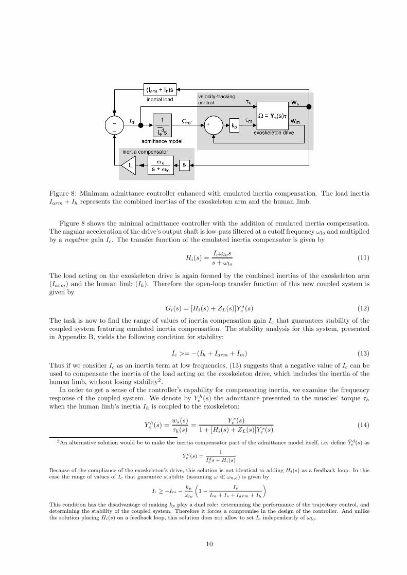
Figure 8: Minimum admittance controller enhanced with emulated inertia compensation. The load inertiaIarm + Ih represents the combined inertias of the exoskeleton arm and the human limb.

Figure 8 shows the minimal admittance controller with the addition of emulated inertia compensation.The angular acceleration of the drive’s output shaft is low-pass filtered at a cutoff frequency ωlo and multipliedby a negative gain Ic. The transfer function of the emulated inertia compensator is given by

Hi(s) =Icωlos

s + ωlo

(11)

The load acting on the exoskeleton drive is again formed by the combined inertias of the exoskeleton arm(Iarm) and the human limb (Ih). Therefore the open-loop transfer function of this new coupled system isgiven by

Gi(s) = [Hi(s) + ZL(s)]Y se (s) (12)

The task is now to find the range of values of inertia compensation gain Ic that guarantees stability of thecoupled system featuring emulated inertia compensation. The stability analysis for this system, presentedin Appendix B, yields the following condition for stability:

Ic >= −(Ih + Iarm + Im) (13)

Thus if we consider Ic as an inertia term at low frequencies, (13) suggests that a negative value of Ic can beused to compensate the inertia of the load acting on the exoskeleton drive, which includes the inertia of thehuman limb, without losing stability2.

In order to get a sense of the controller’s capability for compensating inertia, we examine the frequencyresponse of the coupled system. We denote by Y h

e (s) the admittance presented to the muscles’ torque τh

when the human limb’s inertia Ih is coupled to the exoskeleton:

Y he (s) =

ws(s)

τh(s)=

Y se (s)

1 + [Hi(s) + ZL(s)]Y se (s)

(14)

2An alternative solution would be to make the inertia compensator part of the admittance model itself, i.e. define Y de (s) as

Yde (s) =

1

Ide s + Hi(s)

Because of the compliance of the exoskeleton’s drive, this solution is not identical to adding Hi(s) as a feedback loop. In thiscase the range of values of Ic that guarantee stability (assuming ω ≪ ωn,e) is given by

Ic ≥ −Im −kp

ωlo

(

1 −Is

Im + Is + Iarm + Ih

)

This condition has the disadvantage of making kp play a dual role: determining the performance of the trajectory control, anddetermining the stability of the coupled system. Therefore it forces a compromise in the design of the controller. And unlikethe solution placing Hi(s) on a feedback loop, this solution does not allow to set Ic independently of ωlo.

10

10−1

100

101−20

−10

0

10

20

Mag

nitu

de g

ain

(dB

)

Ic = 0

Ic = −0.4(I

arm+I

h)

Ic = −0.8(I

arm+I

h)

10−1

100

101−180

−90

0

Pha

se (

° )

Frequency (Hz)

10 dB

Figure 9: Frequency-response plots of the closed-loop admittance Y he (s) of the coupled system formed by

the exoskeleton drive with inertia compensation and the load inertia.

Figure 9 shows exemplary frequency-response plots of Y he (s) for different values of Ic. At low frequencies

(i.e. frequencies in the range of human motion), the inertia compensator clearly increases the admittanceof the system. As the frequency increases, all admittances converge to the value corresponding to Ic = 0.Figure 9 shows that for Ic = −0.8(Iarm + Ih) the increase in admittance is about 10 dB at 1 Hz, whichcorresponds to a virtual reduction in load inertia of about 68%. With the values of Iarm and Ih employed,the virtual inertia opposing the muscles will be about 0.54Ih. In other words, wearing the exoskeleton atthat value of Ic should feel similar to reducing the leg segment’s inertia by about half.

Clearly, the model in Figure 8 is a considerable simplification of the physical exoskeleton, but it showsthat the proposed control approach has the potential not only to compensate the inertia of the exoskeleton’sarm, but the inertia of the user’s limb as well.

7 Admittance controller and emulated inertia compensator of the

1-DOF exoskeleton

7.1 Detailed implementation of the admittance controller

The controller implemented for the physical 1-DOF exoskeleton is shown in Figure 10. Its major componentsare an admittance controller and a feedback loop forming the inertia compensator. The admittance controllerconsists of an admittance model followed by a trajectory-tracking LQ controller with an error-integral term[Stengel, 1994]. The admittance model in (1) was converted to the following state space model:

θ

θ

ξ

=

0 1 0

− kde

Ide

− bde

Ide

0

1 0 0

θ

θ

ξ

+

01Id

e

0

τnet (15)

where θ is the angular position of the exoskeleton arm and ξ =∫

θdt. The integral term ξ is employed tominimize tracking error. The input to the admittance model, τnet, is the sum of the torque measured by thetorque sensor, τs, plus the feedback torque from the inertia compensator. The above system can be expressedin compact form as

q = Fd

eq + Gd

eτnet (16)

where q represents the state-space vector

11

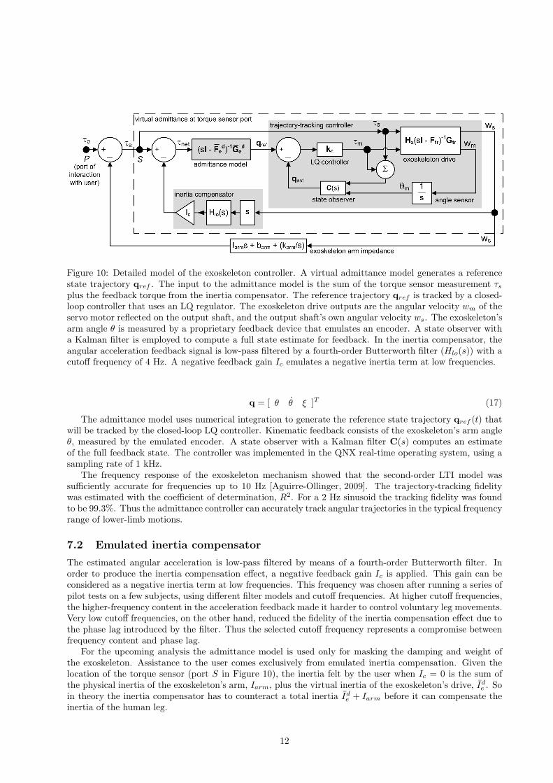
Figure 10: Detailed model of the exoskeleton controller. A virtual admittance model generates a referencestate trajectory qref . The input to the admittance model is the sum of the torque sensor measurement τs

plus the feedback torque from the inertia compensator. The reference trajectory qref is tracked by a closed-loop controller that uses an LQ regulator. The exoskeleton drive outputs are the angular velocity wm of theservo motor reflected on the output shaft, and the output shaft’s own angular velocity ws. The exoskeleton’sarm angle θ is measured by a proprietary feedback device that emulates an encoder. A state observer witha Kalman filter is employed to compute a full state estimate for feedback. In the inertia compensator, theangular acceleration feedback signal is low-pass filtered by a fourth-order Butterworth filter (Hlo(s)) with acutoff frequency of 4 Hz. A negative feedback gain Ic emulates a negative inertia term at low frequencies.

q = [ θ θ ξ ]T (17)

The admittance model uses numerical integration to generate the reference state trajectory qref (t) thatwill be tracked by the closed-loop LQ controller. Kinematic feedback consists of the exoskeleton’s arm angleθ, measured by the emulated encoder. A state observer with a Kalman filter C(s) computes an estimateof the full feedback state. The controller was implemented in the QNX real-time operating system, using asampling rate of 1 kHz.

The frequency response of the exoskeleton mechanism showed that the second-order LTI model wassufficiently accurate for frequencies up to 10 Hz [Aguirre-Ollinger, 2009]. The trajectory-tracking fidelitywas estimated with the coefficient of determination, R2. For a 2 Hz sinusoid the tracking fidelity was foundto be 99.3%. Thus the admittance controller can accurately track angular trajectories in the typical frequencyrange of lower-limb motions.

7.2 Emulated inertia compensator

The estimated angular acceleration is low-pass filtered by means of a fourth-order Butterworth filter. Inorder to produce the inertia compensation effect, a negative feedback gain Ic is applied. This gain can beconsidered as a negative inertia term at low frequencies. This frequency was chosen after running a series ofpilot tests on a few subjects, using different filter models and cutoff frequencies. At higher cutoff frequencies,the higher-frequency content in the acceleration feedback made it harder to control voluntary leg movements.Very low cutoff frequencies, on the other hand, reduced the fidelity of the inertia compensation effect due tothe phase lag introduced by the filter. Thus the selected cutoff frequency represents a compromise betweenfrequency content and phase lag.

For the upcoming analysis the admittance model is used only for masking the damping and weight ofthe exoskeleton. Assistance to the user comes exclusively from emulated inertia compensation. Given thelocation of the torque sensor (port S in Figure 10), the inertia felt by the user when Ic = 0 is the sum ofthe physical inertia of the exoskeleton’s arm, Iarm, plus the virtual inertia of the exoskeleton’s drive, Id

e . Soin theory the inertia compensator has to counteract a total inertia Id

e + Iarm before it can compensate theinertia of the human leg.

12

0.5 1 1.5 2−20

0

20

40

Mag

nitu

de g

ain

(dB

)

αi = [0.7]

αi = [0.6]

αi = [0.53]

0.5 1 1.5 2−90

0

90

180

270

Pha

se (

° )

Frequency (Hz)

gain margin < 0

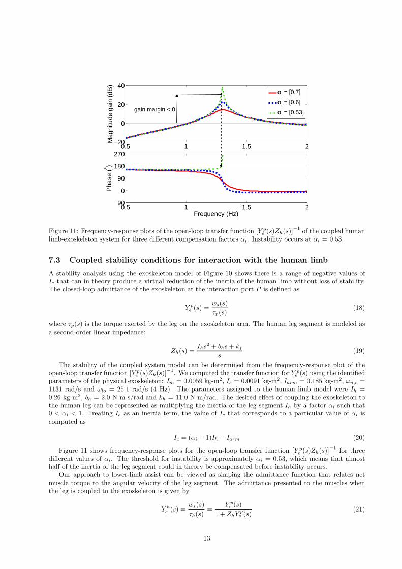
Figure 11: Frequency-response plots of the open-loop transfer function [Y pe (s)Zh(s)]

−1of the coupled human

limb-exoskeleton system for three different compensation factors αi. Instability occurs at αi = 0.53.

7.3 Coupled stability conditions for interaction with the human limb

A stability analysis using the exoskeleton model of Figure 10 shows there is a range of negative values ofIc that can in theory produce a virtual reduction of the inertia of the human limb without loss of stability.The closed-loop admittance of the exoskeleton at the interaction port P is defined as

Y pe (s) =

ws(s)

τp(s)(18)

where τp(s) is the torque exerted by the leg on the exoskeleton arm. The human leg segment is modeled asa second-order linear impedance:

Zh(s) =Ihs2 + bhs + kj

s(19)

The stability of the coupled system model can be determined from the frequency-response plot of theopen-loop transfer function [Y p

e (s)Zh(s)]−1

. We computed the transfer function for Y pe (s) using the identified

parameters of the physical exoskeleton: Im = 0.0059 kg-m2, Is = 0.0091 kg-m2, Iarm = 0.185 kg-m2, ωn,e =1131 rad/s and ωlo = 25.1 rad/s (4 Hz). The parameters assigned to the human limb model were Ih =0.26 kg-m2, bh = 2.0 N-m-s/rad and kh = 11.0 N-m/rad. The desired effect of coupling the exoskeleton tothe human leg can be represented as multiplying the inertia of the leg segment Ih by a factor αi such that0 < αi < 1. Treating Ic as an inertia term, the value of Ic that corresponds to a particular value of αi iscomputed as

Ic = (αi − 1)Ih − Iarm (20)

Figure 11 shows frequency-response plots for the open-loop transfer function [Y pe (s)Zh(s)]

−1for three

different values of αi. The threshold for instability is approximately αi = 0.53, which means that almosthalf of the inertia of the leg segment could in theory be compensated before instability occurs.

Our approach to lower-limb assist can be viewed as shaping the admittance function that relates netmuscle torque to the angular velocity of the leg segment. The admittance presented to the muscles whenthe leg is coupled to the exoskeleton is given by

Y he (s) =

ws(s)

τh(s)=

Y pe (s)

1 + ZhYpe (s)

(21)

13

0.5 1 1.5 2−15

−10

−5

0

5

10

Mag

nitu

de g

ain

(dB

)

0.5 1 1.5 2

90

0

−90

Pha

se (

° )

Frequency (Hz)

αi = [0.7]

αi = [0.6]

αi = [0.53]

Zh−1(s)

~11 dB

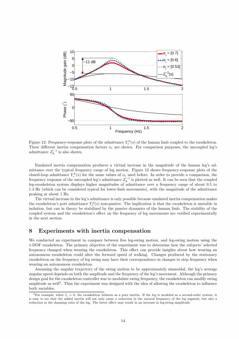
Figure 12: Frequency-response plots of the admittance Y he (s) of the human limb coupled to the exoskeleton.

Three different inertia compensation factors αi are shown. For comparison purposes, the uncoupled leg’sadmittance Z−1

h is also shown.

Emulated inertia compensation produces a virtual increase in the magnitude of the human leg’s ad-mittance over the typical frequency range of leg motion. Figure 12 shows frequency-response plots of theclosed-loop admittance Y h

e (s) for the same values of αi used before. In order to provide a comparison, thefrequency response of the uncoupled leg’s admittance Z−1

h is plotted as well. It can be seen that the coupledleg-exoskeleton system displays higher magnitudes of admittance over a frequency range of about 0.5 to1.4 Hz (which can be considered typical for lower-limb movements), with the magnitude of the admittancepeaking at about 1 Hz.

The virtual increase in the leg’s admittance is only possible because emulated inertia compensation makesthe exoskeleton’s port admittance Y p

e (s) non-passive. The implication is that the exoskeleton is unstable inisolation, but can in theory be stabilized by the passive dynamics of the human limb. The stability of thecoupled system and the exoskeleton’s effect on the frequency of leg movements are verified experimentallyin the next section.

8 Experiments with inertia compensation

We conducted an experiment to compare between free leg-swing motion, and leg-swing motion using the1-DOF exoskeleton. The primary objective of the experiment was to determine how the subjects’ selectedfrequency changed when wearing the exoskeleton. This effect can provide insights about how wearing anautonomous exoskeleton could alter the forward speed of walking. Changes produced by the stationaryexoskeleton on the frequency of leg swing may have their correspondence in changes to step frequency whenwearing an autonomous exoskeleton.

Assuming the angular trajectory of the swing motion to be approximately sinusoidal, the leg’s averageangular speed depends on both the amplitude and the frequency of the leg’s movement. Although the primarydesign goal for the exoskeleton controller was to modulate swing frequency, the exoskeleton can modify swingamplitude as well3. Thus the experiment was designed with the idea of allowing the exoskeleton to influenceboth variables.

3For example, when Ic = 0, the exoskeleton behaves as a pure inertia. If the leg is modeled as a second-order system, itis easy to see that the added inertia will ont only cause a reduction in the natural frequency of the leg segment, but also areduction in the damping ratio of the leg. The latter effect may result in an increase in leg-swing amplitude.

14

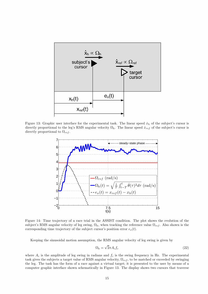
Figure 13: Graphic user interface for the experimental task. The linear speed xh of the subject’s cursor isdirectly proportional to the leg’s RMS angular velocity Ωh. The linear speed xref of the subject’s cursor isdirectly proportional to Ωref .

0 7.5 15−2

−1

0

1

2

3

4

5

6

7

t(s)

Ωref (rad/s)

Ωh(t) =√

1T

∫ t

t−Tθ(τ)2dτ (rad/s)

ex(t) = xref (t) − xh(t)

steady−state phase

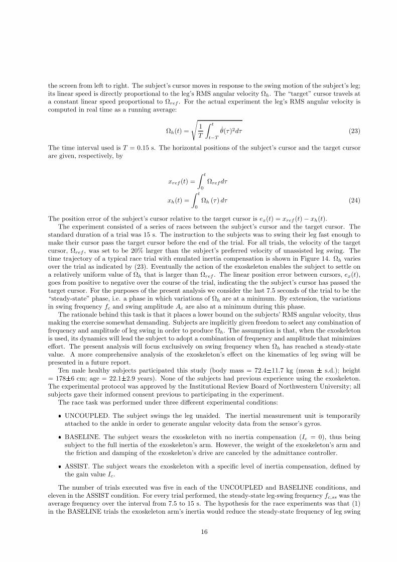
Figure 14: Time trajectory of a race trial in the ASSIST condition. The plot shows the evolution of thesubject’s RMS angular velocity of leg swing, Ωh, when tracking the reference value Ωref . Also shown is thecorresponding time trajectory of the subject cursor’s position error ex(t).

Keeping the sinusoidal motion assumption, the RMS angular velocity of leg swing is given by

Ωh =√

2πAcfc (22)

where Ac is the amplitude of leg swing in radians and fc is the swing frequency in Hz. The experimentaltask gives the subjects a target value of RMS angular velocity, Ωref , to be matched or exceeded by swingingthe leg. The task has the form of a race against a virtual target; it is presented to the user by means of acomputer graphic interface shown schematically in Figure 13. The display shows two cursors that traverse

15

the screen from left to right. The subject’s cursor moves in response to the swing motion of the subject’s leg;its linear speed is directly proportional to the leg’s RMS angular velocity Ωh. The “target” cursor travels ata constant linear speed proportional to Ωref . For the actual experiment the leg’s RMS angular velocity iscomputed in real time as a running average:

Ωh(t) =

√

1

T

∫ t

t−T

θ(τ)2dτ (23)

The time interval used is T = 0.15 s. The horizontal positions of the subject’s cursor and the target cursorare given, respectively, by

xref (t) =

∫ t

0

Ωrefdτ

xh(t) =

∫ t

0

Ωh (τ) dτ (24)

The position error of the subject’s cursor relative to the target cursor is ex(t) = xref (t) − xh(t).The experiment consisted of a series of races between the subject’s cursor and the target cursor. The

standard duration of a trial was 15 s. The instruction to the subjects was to swing their leg fast enough tomake their cursor pass the target cursor before the end of the trial. For all trials, the velocity of the targetcursor, Ωref , was set to be 20% larger than the subject’s preferred velocity of unassisted leg swing. Thetime trajectory of a typical race trial with emulated inertia compensation is shown in Figure 14. Ωh variesover the trial as indicated by (23). Eventually the action of the exoskeleton enables the subject to settle ona relatively uniform value of Ωh that is larger than Ωref . The linear position error between cursors, ex(t),goes from positive to negative over the course of the trial, indicating the the subject’s cursor has passed thetarget cursor. For the purposes of the present analysis we consider the last 7.5 seconds of the trial to be the“steady-state” phase, i.e. a phase in which variations of Ωh are at a minimum. By extension, the variationsin swing frequency fc and swing amplitude Ac are also at a minimum during this phase.

The rationale behind this task is that it places a lower bound on the subjects’ RMS angular velocity, thusmaking the exercise somewhat demanding. Subjects are implicitly given freedom to select any combination offrequency and amplitude of leg swing in order to produce Ωh. The assumption is that, when the exoskeletonis used, its dynamics will lead the subject to adopt a combination of frequency and amplitude that minimizeseffort. The present analysis will focus exclusively on swing frequency when Ωh has reached a steady-statevalue. A more comprehensive analysis of the exoskeleton’s effect on the kinematics of leg swing will bepresented in a future report.

Ten male healthy subjects participated this study (body mass = 72.4±11.7 kg (mean ± s.d.); height= 178±6 cm; age = 22.1±2.9 years). None of the subjects had previous experience using the exoskeleton.The experimental protocol was approved by the Institutional Review Board of Northwestern University; allsubjects gave their informed consent previous to participating in the experiment.

The race task was performed under three different experimental conditions: UNCOUPLED. The subject swings the leg unaided. The inertial measurement unit is temporarilyattached to the ankle in order to generate angular velocity data from the sensor’s gyros. BASELINE. The subject wears the exoskeleton with no inertia compensation (Ic = 0), thus beingsubject to the full inertia of the exoskeleton’s arm. However, the weight of the exoskeleton’s arm andthe friction and damping of the exoskeleton’s drive are canceled by the admittance controller. ASSIST. The subject wears the exoskeleton with a specific level of inertia compensation, defined bythe gain value Ic.

The number of trials executed was five in each of the UNCOUPLED and BASELINE conditions, andeleven in the ASSIST condition. For every trial performed, the steady-state leg-swing frequency fc,ss was theaverage frequency over the interval from 7.5 to 15 s. The hypothesis for the race experiments was that (1)in the BASELINE trials the exoskeleton arm’s inertia would reduce the steady-state frequency of leg swing

16

(a) BAS vs. UNC (b) ASST vs. BAS (c) ASST vs. UNC−0.2

−0.15

−0.1

−0.05

0

0.05

0.1

0.15

0.2

−0.133 ± 0.041 Hz(−12.99 ± 4.08 %)

0.135 ± 0.027 Hz(13.87 ± 2.99 %)

0.002 ± 0.060 Hz(0.88 ± 6.34 %)

∆fc,

ss (

Hz)

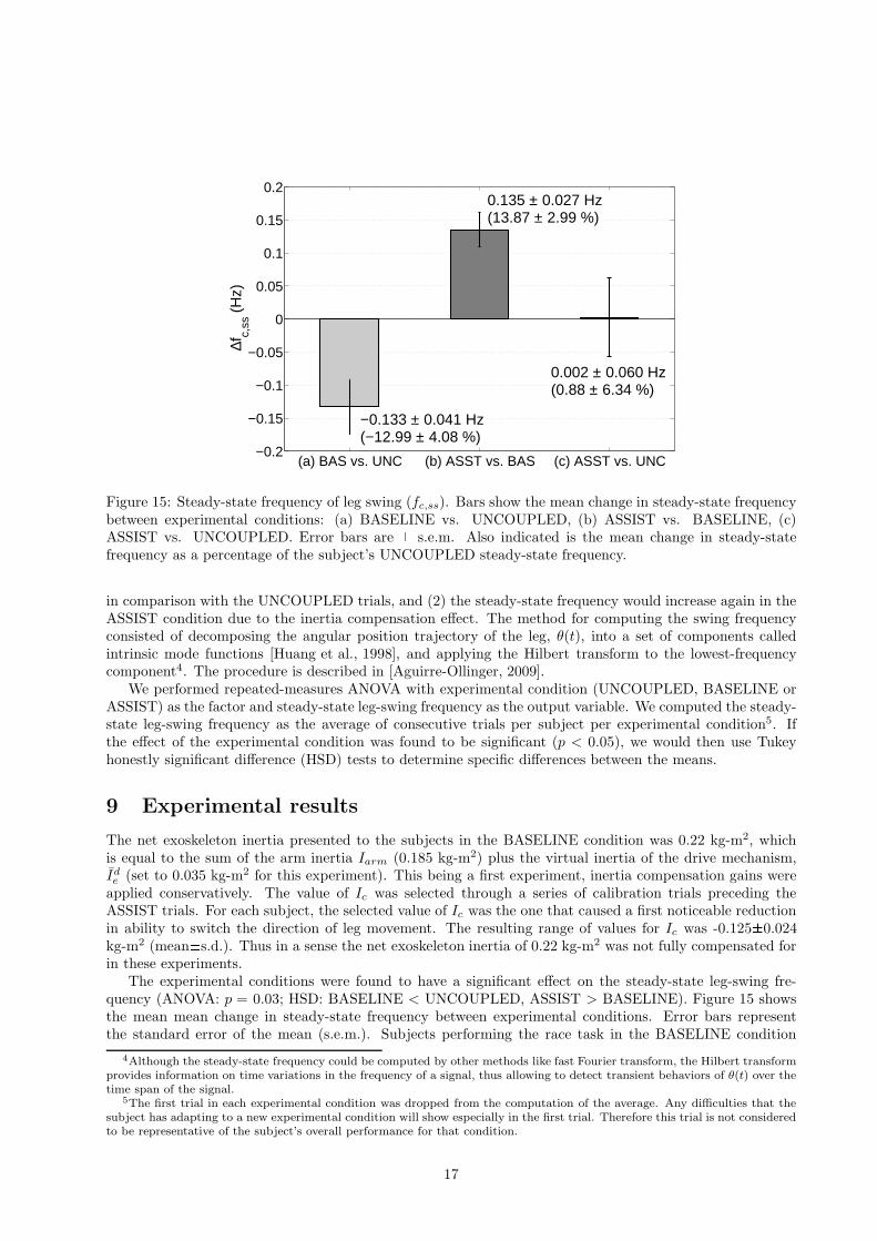
Figure 15: Steady-state frequency of leg swing (fc,ss). Bars show the mean change in steady-state frequencybetween experimental conditions: (a) BASELINE vs. UNCOUPLED, (b) ASSIST vs. BASELINE, (c)ASSIST vs. UNCOUPLED. Error bars are ± s.e.m. Also indicated is the mean change in steady-statefrequency as a percentage of the subject’s UNCOUPLED steady-state frequency.

in comparison with the UNCOUPLED trials, and (2) the steady-state frequency would increase again in theASSIST condition due to the inertia compensation effect. The method for computing the swing frequencyconsisted of decomposing the angular position trajectory of the leg, θ(t), into a set of components calledintrinsic mode functions [Huang et al., 1998], and applying the Hilbert transform to the lowest-frequencycomponent4. The procedure is described in [Aguirre-Ollinger, 2009].

We performed repeated-measures ANOVA with experimental condition (UNCOUPLED, BASELINE orASSIST) as the factor and steady-state leg-swing frequency as the output variable. We computed the steady-state leg-swing frequency as the average of consecutive trials per subject per experimental condition5. Ifthe effect of the experimental condition was found to be significant (p < 0.05), we would then use Tukeyhonestly significant difference (HSD) tests to determine specific differences between the means.

9 Experimental results

The net exoskeleton inertia presented to the subjects in the BASELINE condition was 0.22 kg-m2, whichis equal to the sum of the arm inertia Iarm (0.185 kg-m2) plus the virtual inertia of the drive mechanism,Ide (set to 0.035 kg-m2 for this experiment). This being a first experiment, inertia compensation gains were

applied conservatively. The value of Ic was selected through a series of calibration trials preceding theASSIST trials. For each subject, the selected value of Ic was the one that caused a first noticeable reductionin ability to switch the direction of leg movement. The resulting range of values for Ic was -0.125±0.024kg-m2 (mean±s.d.). Thus in a sense the net exoskeleton inertia of 0.22 kg-m2 was not fully compensated forin these experiments.

The experimental conditions were found to have a significant effect on the steady-state leg-swing fre-quency (ANOVA: p = 0.03; HSD: BASELINE < UNCOUPLED, ASSIST > BASELINE). Figure 15 showsthe mean mean change in steady-state frequency between experimental conditions. Error bars representthe standard error of the mean (s.e.m.). Subjects performing the race task in the BASELINE condition

4Although the steady-state frequency could be computed by other methods like fast Fourier transform, the Hilbert transformprovides information on time variations in the frequency of a signal, thus allowing to detect transient behaviors of θ(t) over thetime span of the signal.

5The first trial in each experimental condition was dropped from the computation of the average. Any difficulties that thesubject has adapting to a new experimental condition will show especially in the first trial. Therefore this trial is not consideredto be representative of the subject’s overall performance for that condition.

17

showed a considerable reduction in swing frequency with respect to the UNCOUPLED case (-12.99±4.08%).This reduction is consistent with the exoskeleton arm’s inertia reducing the natural frequency of the leg.The ASSIST condition in turn increased the steady-state frequency with respect to the BASELINE case(13.87±2.99%), suggesting that emulated inertia compensation effectively counteracts the arm’s inertia.There was no significant difference between steady-state frequencies for the ASSIST and UNCOUPLEDconditions (0.88±6.34%). Thus for practical purposes inertia compensation brought the natural frequencyof the leg back to levels corresponding to those of unassisted leg. Interestingly, this result was achieved withinertia compensation gains Ic that in theory was not large enough in magnitude to fully compensate theinertia of the exoskeleton, let alone compensate the inertia of the human limb.

It is instructive to examine the differences in the exoskeleton’s measured impedance between the BASE-LINE and ASSIST conditions. We computed the impedance at the torque sensor port at the mean steady-state frequency of leg swing. The impedance was obtained from the fast Fourier transforms of the measuredtorque, τs, and the measured angular velocity, ws. The mean impedance value was -0.257 + 1.031i N-m-s/rad for the BASELINE condition6. The mean impedance value for the ASSIST condition was -0.667 +0.450i N-m-s/rad. Thus the real part of the impedance becomes more negative when inertia compensation ispresent. In other words, the emulated inertia compensator, besides modulating the frequency of swing, alsoadds negative damping. As a consequence the exoskeleton in the ASSIST condition produces a net transferof energy to the user’s leg.

10 Discussion

We have developed a control method that, in a sense, goes against conventional thinking about human-robotinteraction. Impedance and admittance control methods for human-robot interaction typically emphasizecoupled stability. Robot passivity has been long established as a condition for guaranteed coupled stabil-ity between the robot and any passive environment [Colgate and Hogan, 1989, Colgate and Hogan, 1988].However, our strategy for lower-limb assist is based on making the exoskeleton produce a virtual increase inthe leg’s admittance. This can only be accomplished if the exoskeleton exhibits non-passive behavior, withthe implication that the exoskeleton is unstable in isolation. Stable interaction between the exoskeleton andthe lower extremities is possible due in part to the passive dynamics of the leg. However, the role of humansensorimotor control needs to be considered as well. Burdet [Burdet et al., 2001] has reported that humansadapt well to unstable manual tasks when perturbation forces are normal to the direction of the intendedmotion. In the case of an active exoskeleton, destabilizing forces act on the direction of the desired motion.The human’s mechanism for adapting to such forces is a potential area of research.

In the experiments reported here, user safety was given preeminence over performance. Thus the iner-tia compensation gains (Ic) were applied conservatively. We found that subjects consistently reduced thefrequency of leg swing in the exoskeleton’s BASELINE condition, but were able to recover their normalfrequency of leg swing when inertia compensation was applied. Surprisingly, this effect was accomplishedwith inertia compensation gains that on average were 43% smaller than the theoretical value needed to fullycompensate the inertia of the exoskeleton. This larger-than-expected increase in frequency may be explainedby an attendant increase in the level of co-contraction of the muscles controlling flexion and extension ofthe knee joint. A high level of co-contraction would increase the stiffness of the leg joint, thus making anadditional contribution to raising the natural frequency of the limb segment. Using EMG measurements infuture experiments may clarify whether an increase in co-contraction actually occurs.

While in general the swing frequencies achieved by the subjects in the ASSIST condition were not largerthan in the UNCOUPLED case, we did not find anything to suggest that larger negative values of Ic cannotbe employed in future experiments. The key is probably to run longer series of trials, giving the subjectsmore time to adapt to the exoskeleton’s dynamics. In a few separate trials we have had subjects interactcomfortably with the exoskeleton at Ic gains as large as -0.24 kg-m2.

The implementation discussed here was restricted to single-joint control, but it can in principle be trans-ferred to multi-joint control. Emulated inertia compensation is expected to have an effect on the swing phase

6Although the exoskeleton in the BASELINE condition (Ic = 0) is theoretically passive at the interaction port P (see Figure10), a negative value of virtual damping b

de is necessary to mask the physical damping of the arm. Hence the negative real part

(-0.257 N-m-s/rad) of the measured impedance.

18

of walking. Therefore, the design we envision for a wearable exoskeleton is a hip-mounted device with actu-ators assisting leg motion on the sagittal plane. Hip abduction/adduction may be allowed by an unactuateddegree of freedom of the mechanism. Such a design avoids placing distal masses on the leg, thereby reducingthe handicap on agility associated with loading the leg [Browning et al., 2007, Royer and Martin, 2005].

The cable drive transmission performed remarkably well in producing an active admittance behaviorwithout the issue of limit cycles. However, there is a limit to the transmission ratio that can be achievedby a cable drive, which in turn may require the use of a relatively large actuator in order to assist walking.However, this might offset the expected reduction in metabolic cost during leg swing. The mass added bythe exoskeleton at the subject’s center of mass (COM) can increase the metabolic cost of redirecting theCOM at each step [Donelan et al., 2002]. A highly geared transmission could allow the use of less massivemotors, however at the cost of having to solve the limit-cycle issue in control rather than hardware.

11 Conclusions

Our approach to exoskeleton control is based on making the exoskeleton shape the dynamics of the humanlimb. This paper focused on one particular strategy for lower-limb assist: compensating the inertia of thelegs in order to increase their natural frequency. To achieve this effect, the controller has to first overcome thehandicap introduced by the exoskeleton’s own inertia, which tends to actually reduce the natural frequencyof the legs.

Admittance control is a well-established method for masking the stiffness and the damping of a me-chanical system [Newman, 1992]. However, non-collocation of the torque sensor makes it unfeasible for theexoskeleton to follow an admittance model with a negative inertia term. Instead, we have emulated inertiacompensation through positive feedback of the low-pass filtered angular acceleration. The effect resemblesinertia compensation in that it produces a virtual increase in the magnitude of the human leg’s admittanceat typical frequencies of leg motion. Emulated inertia compensation makes the exoskeleton exhibit activeadmittance, and thus behave as a source of mechanical energy to the human limbs. Although active ad-mittance makes the exoskeleton unstable in isolation, subjects in our experiment were able to adapt to thedestabilizing effects of the exoskeleton, and increase their frequency of leg swing in the process. However, theeffects of wearing the exoskeleton on muscle activation and metabolic consumption have yet to be studied.

The main application we envision for our active-admittance control is assisting the swing phase of walking.For our future research we plan to develop a wearable exoskeleton to test the effects of inertia compensationon actual walking. Specific research objectives include determining how the exoskeleton affects the user’sselected combination of step frequency and step length, and determining whether inertia compensation canenable walking at higher speeds with a metabolic cost lower than that corresponding to unassisted walking.

Funding

This work was supported by the Honda Research Institute (Mountain View, CA).

A Stability of a simple con-collocated system under admittance

control

We begin by testing G(s) in (8) for right half-plane poles. The characteristic polynomial of G(s) yields thefollowing Routh array:

[

1,kp

Im, kc

Im,

kpkc

ImIs

]

(25)

Because all the coefficients involved are positive, no changes of sign occur in the Routh array. In consequencethe open-loop transfer function G(s) has no right half-plane poles. Therefore, a sufficient condition for thestability of the closed-loop system is that G(s) produces no encirclements of -1. The task is therefore to findthe range of values of of Id

e that simultaneously satisfy

19

ReG(jω) > −1

ImG(jω) = 0 (26)

G(jω) is given by

G(jω) =a(ω) + jb(ω)

c(ω) + jd(ω)(27)

where

a(ω) = Ide Im(Iarm + Ih)ω4 − kcI

de (Iarm + Ih)ω2

b(ω) = −Ide kp(Iarm + Ih)ω3 + kpkc(Iarm + Ih)ω

c(ω) = Ide ImIsω

4 − Ide kc(Im + Is)ω

2

d(ω) = −kpIsIde ω3 + kpkcI

de ω (28)

From (26) we can derive the following system of equations:

a(ω)c(ω) + b(ω)d(ω)

c(ω)2 + d(ω)2> −1

b(ω)c(ω) − a(ω)d(ω)

c(ω)2 + d(ω)2= 0 (29)

After solving (29) for Ide and ω we arrive at the following stability condition:

Ide ≥ Im(Iarm + Ih)

Is + Iarm + Ih

(30)

B Stability of a simple con-collocated system with emulated iner-

tia compensation

We will restrict the analysis to the limit case Ide = Im. Substituting terms in (12) yields the following

expression for the open-loop transfer function:

Gi(s) = Ki

Ni(s)

Di(s)(31)

where

20

Ki =Iarm + Ih

Is

Ni(s) = s4

+kp(Ih + Iarm) + ωloIm(Iarm + Ih + Ic))

Im(Iarm + Ih)s3

+ω2

n,eImIs(Iarm + Ih) + ωlokp(Im + Is)(Iarm + Ih + Ic)

Im(Im + Is)(Iarm + Ih)s2

+ω2

n,eIs(kp(Iarm + Ih) + ωloIm(Iarm + Ih + Ic))

Im(Im + Is)(Iarm + Ih)s

+ωloω

2n,ekpIs(Iarm + Ih + Ic)

Im(Im + Is)(Iarm + Ih)

Di(s) = s4 +kp + ωloIm

Im

s3 +ωlokp + ω2

n,eIm

Im

s2

+ω2

n,e(kp + ωlo(Im + Is))

Im + Is

s +ωlokpω

2n,e

Im + Is

(32)

In the above equations ωn,e is the natural frequency of the exoskeleton drive, given by

ωn,e =

√

kc(Im + Is)

ImIs

(33)

The Routh array of Di(s) in (32) is

[

1,ωloIm+kp

Im,

kpωlo+ω2

n,eIm

Im,

ω2

n,e(kp+ωlo(Im+Is))

Im+Is,

ωloω2

n,ekp

Im+Is

]

(34)

Because no changes of sign occur in the Routh array, it follows that Gi(s) has no right half-plane poles.Therefore, as in the previous analysis, a sufficient condition for stability is that the open-loop transferfunction produces no encirclements of -1. The analysis can be simplified considerably by limiting it to thecase ω ≪ ωn,e, which yields the following expression for Gi(jω):

Gi(jω) =ai(ω) + jbi(ω)

ci(ω) + jdi(ω)(35)

where

ai(ω) = −ImIs[Iarm(kp + ωloIm) + Ihkp + ωloIm(Ih + Ic)]ω2

bi(ω) = −I2mIs(Iarm + Ih)ω3 + ImIsωlokp(Iarm + Ih + Ic)ω

ci(ω) = −I2mIs[kp + ωlo(Im + Is)]ω

2

di(ω) = −I2mIs(Im + Is)ω

3 + ωlokpI2mIsω (36)

Solving for ReGi(jω) > −1 and ImGi(jω) = 0 yields the following condition:

Ic >= −(Ih + Iarm + Im) (37)

References

[Aguirre-Ollinger, 2009] Aguirre-Ollinger, G. (2009). Active Impedance Control of a Lower-Limb AssistiveExoskeleton. dissertation, Northwestern University, Evanston, IL.

21

[Aguirre-Ollinger et al., 2007a] Aguirre-Ollinger, G., Colgate, J., Peshkin, M., and Goswami, A. (2007a). A1-dof assistive exoskeleton with virtual negative damping: effects on the kinematic response of the lowerlimbs. In Intelligent Robots and Systems, 2007. IROS 2007. IEEE/RSJ International Conference on,pages 1938 –1944.

[Aguirre-Ollinger et al., 2007b] Aguirre-Ollinger, G., Colgate, J., Peshkin, M., and Goswami, A. (2007b).Active-impedance control of a lower-limb assistive exoskeleton. In Rehabilitation Robotics, 2007. ICORR2007. IEEE 10th International Conference on, pages 188 –195.

[Banala et al., 2006] Banala, S., Agrawal, S. K., Fattah, A., Krishnamoorthy, V., Hsu, W.-L., Scholz, J., andRudolph, K. (2006). Gravity-balancing leg orthosis and its performance evaluation. IEEE Transactionson Robotics, 22(6):1228–1239.

[Banala et al., 2009] Banala, S., Kim, S., Agrawal, S., and Scholz, J. (2009). Robot assisted gait trainingwith active leg exoskeleton (ALEX). Neural Systems and Rehabilitation Engineering, IEEE Transactionson, 17(1):2–8.

[Browning et al., 2007] Browning, R. C., Modica, J. R., Kram, R., and Goswami, A. (2007). The effects ofadding mass to the legs on the energetics and biomechanics of walking. Medicine and Science in Sportsand Exercise, 39(3):515–525.

[Buerger and Hogan, 2007] Buerger, S. and Hogan, N. (2007). Complementary stability and loop shapingfor improved human-robot interaction. Robotics, IEEE Transactions on, 23(2):232–244.

[Burdet et al., 2001] Burdet, E., Osu, R., Franklin, D., Milner, T., and Kawato, M. (2001). The centralnervous system stabilizes unstable dynamics by learning optimal impedance. Nature, 414:446–449.

[Colgate and Hogan, 1989] Colgate, E. and Hogan, N. (1989). The interaction of robots with passive envi-ronments: Application to force feedback control. Fourth International Conference on Advanced Robotics.

[Colgate and Hogan, 1988] Colgate, J. and Hogan, N. (1988). Robust control of dynamically interactingsystems. International Journal of Control, 48(1):65–88.

[DeVita and Hortobagyi, 2003] DeVita, P. and Hortobagyi, T. (2003). Obesity is not associated with in-creased knee joint torque and power during level walking. Journal of Biomechanics, 36:1355–1362.

[Doke et al., 2005] Doke, J., Donelan, J. M., and Kuo, A. D. (2005). Mechanics and energetics of swingingthe human leg. Journal of Experimental Biology, 208:439–445.

[Dollar and Herr, 2008] Dollar, A. and Herr, H. (2008). Lower extremity exoskeletons and active orthoses:Challenges and state of the art. IEEE Transactions on Robotics, 24(1):144–158.

[Donelan et al., 2002] Donelan, J., Kram, R., and Kuo, A. (2002). Mechanical work for step-to-step transi-tions is a major determinant of the metabolic cost of human walking. Journal of Experimental Biology,205:3717–3727.

[Ferris et al., 2007] Ferris, D., Sawicki, G., and Daley, M. (2007). A physiologist’s perspective on roboticexoskeletons for human locomotion. International Journal of Humanoid Robotics, 4:507–528.

[Ferris et al., 2005] Ferris, D., Sawicki, G., and Domingo, A. (2005). Powered lower limb orthoses for gaitrehabilitation. Top Spinal Cord Inj Rehabil, 11(2):34–49.

[Huang et al., 1998] Huang, N., Shen, Z., Long, S., Wu, M., Shih, H., Zheng, Q., Yen, N., Tung, C., and Liu,H. (1998). The empirical mode decomposition and the Hilbert spectrum for nonlinear and non-stationarytime series analysis. Proc. R. Soc. Lond. A, 454:903–995.

[Jezernik et al., 2004] Jezernik, S., Colombo, G., and Morari, M. (2004). Automatic gait-pattern adaptationalgorithms for rehabilitation with a 4-dof robotic orthosis. IEEE Transactions on Robotics and Automation,20(3):574–582.

22

[Kawamoto and Sankai, 2005] Kawamoto, H. and Sankai, Y. (2005). Power assist method based on phasesequence and muscle force condition for HAL. Advanced Robotics, 19(7):717–734.

[Kazerooni et al., 2005] Kazerooni, H., Racine, J.-L., Huang, L., and Steger, R. (2005). On the controlof the berkeley lower extremity exoskeleton (BLEEX). In Robotics and Automation, 2005. ICRA 2005.Proceedings of the 2005 IEEE International Conference on, pages 4353 – 4360.

[Kerrigan et al., 2000] Kerrigan, D., Riley, P., Nieto, T. J., and Della Croce, U. (2000). Knee joint torques:A comparison between women and men during barefoot walking. Arch. Phys. Med. Rehabil, 81:1162–1165.

[Kuo, 2001] Kuo, A. D. (2001). A simple model of bipedal walking predicts the preferred speed–step lengthrelationship. Journal of Biomechanical Engineering, 123(3):264–269.

[Lee and Sankai, 2002] Lee, S. and Sankai, Y. (2002). Power assist control for walking aid with HAL-3based on EMG and impedance adjustment around knee joint. In Intelligent Robots and Systems, 2002.IEEE/RSJ International Conference on, volume 2, pages 1499 – 1504 vol.2.

[Lee and Sankai, 2003] Lee, S. and Sankai, Y. (2003). The natural frequency-based power assist control forlower body with HAL-3. IEEE International Conference on Systems, Man and Cybernetics, 2:1642–1647.

[Lee and Sankai, 2005] Lee, S. and Sankai, Y. (2005). Virtual impedance adjustment in unconstrained mo-tion for an exoskeletal robot assisting the lower limb. Advanced Robotics, 19(7):773–795.

[Newman, 1992] Newman, W. (1992). Stability and performance limits of interaction controllers. Journalof Dynamic Systems, Measurement, and Control, 114(4):563–570.

[Royer and Martin, 2005] Royer, T. D. and Martin, P. E. (2005). Manipulations of leg mass and moment ofinertia: Effects on energy cost of walking. Medicine and Science in Sports and Exercise, 37(4):649–656.

[Sawicki and Ferris, 2009] Sawicki, G. and Ferris, D. (2009). Powered ankle exoskeletons reveal the metaboliccost of plantar flexor mechanical work during walking with longer steps at constant step frequency. Journalof Experimental Biology, 212:21–31.

[Stengel, 1994] Stengel, R. (1994). Optimal Control and Estimation. Dover Publications, Inc., New York,NY.

[Uemura et al., 2006] Uemura, M., Kanaoka, K., and Kawamura, S. (2006). Power assist systems based onresonance of passive elements. In Intelligent Robots and Systems, 2006 IEEE/RSJ International Confer-ence on, pages 4316 –4321.

[Veneman et al., 2007] Veneman, J., Kruidhof, R., Hekman, E., Ekkelenkamp, R., Van Asseldonk, E., andvan der Kooij, H. (2007). Design and evaluation of the lopes exoskeleton robot for interactive gait reha-bilitation. Neural Systems and Rehabilitation Engineering, IEEE Transactions on, 15(3):379–386.

[Walsh et al., 2006] Walsh, C., Paluska, D., Pasch, K., Grand, W., Valiente, A., and Herr, H. (2006). De-velopment of a lightweight, underactuated exoskeleton for load-carrying augmentation. In Robotics andAutomation, 2006. ICRA 2006. Proceedings 2006 IEEE International Conference on, pages 3485 –3491.

23