design and analysis of delivery ‘pipelines’ in truckload trucking

Transportation Research Part E 45 (2009) 255–269

Contents lists available at ScienceDirect

Transportation Research Part E

journal homepage: www.elsevier .com/locate / t re

Design and analysis of delivery ‘pipelines’ in truckload trucking

G. Don Taylor a,*, Gary L. Whicker b, W. Grant DuCote b

a Department of Industrial and Systems Engineering, Virginia Polytechnic Institute and State University, Blacksburg, VA 24061, USAb J.B. Hunt Transport, Inc., P.O. Box 130, 615 J.B. Hunt Corporate Drive, Lowell, AR 72745, USA

a r t i c l e i n f o a b s t r a c t

Article history:Received 24 June 2005Received in revised form 3 November 2005Accepted 10 January 2006

Keywords:DispatchingDriver managementTruckload trucking

1366-5545/$ - see front matter � 2008 Elsevier Ltddoi:10.1016/j.tre.2006.01.006

* Corresponding author.E-mail address: [email protected] (G. Don Taylo

This paper examines a new dispatching alternative for the truckload trucking industryinvolving the use of delivery ‘pipelines’ with dense flow volumes. Drivers and loads arepartitioned into two sets; those that utilize pipelines via a series of ‘dray’ moves andline-hauls, and the remaining set of random over-the-road (OTR) drivers that are dis-patched by traditional methods. Alternative methods are presented to determine wheredelivery pipelines should be located and how they should be operated. The effects of thepipelines on the remaining OTR fleet are also examined. Results indicate that the new dis-patching alternative is feasible.

� 2008 Elsevier Ltd. All rights reserved.

1. Introduction and motivation

In the United States, the truckload trucking industry is highly competitive. With more than 600,000 registered motor car-riers (United States Department of Transportation, 2005), profit margins are low and shippers often wait until the last minuteto secure a carrier. This customer behavior results in a seemingly random set of dispatching needs and a general lack ofadvance information that might be exploited by dispatching systems. This operating environment adds considerably tothe difficulty of the already daunting dispatching problem in support of random over-the-road (OTR) operations.

To complicate the dispatching task further, carriers must consider their own needs while they concurrently consider theneeds of customers and drivers. The desire for cost effective dispatching decisions often leads carriers to dispatch drivers bymethods that focus heavily on the minimization of empty relocation miles between loads. This methodology, however, canlead to excessively long tour lengths for drivers. This affects the quality of driver life and is a leading cause of driver turnoverin an industry that considers one of its most difficult challenges to be that of retaining drivers (see, for example, Schwartz,1992 or Richardson, 1994). The driver shortage is so acute that some researchers such as Min and Emam (2003) performresearch to find which driver characteristics make them more likely to stay on the job. They then use data mining techniquesto develop ways to recruit and retain drivers with those characteristics. Griffin et al. (2000) list a number of important factorsin retaining drivers. Key among these factors is the location of the carrier home base, the amount of time at home, and thequality of routes that they drive. To better support driver needs for more frequent domicile returns, a great deal of recentresearch has focused on finding better ways to dispatch drivers. Sabnani and Hall (2002) designate specific driving routesthat remain in effect for weeks or even months. This work is in the less-than-truckload environment, but the idea is soundin truckload trucking as well. Another possible way to defeat the challenges associated with driver retention would be to findalternative means of dispatching that could be used for all or part of existing OTR driving fleets.

In this paper, the authors consider the development of a dispatching alternative using driving ‘pipelines’ that would bethe trucking equivalent of the railway portion of an intermodal shipment. These pipelines would utilize existing highway

. All rights reserved.

r).

mailto:[email protected]

http://www.sciencedirect.com/science/journal/13665545

http://www.elsevier.com/locate/tre

Pipeline

DrayMoves

DrayMoves

Domicile and Drop/Swap Points

C

B

A

Fig. 1. Graphical example of ‘pipeline’ operations.

256 G. Don Taylor et al. / Transportation Research Part E 45 (2009) 255–269

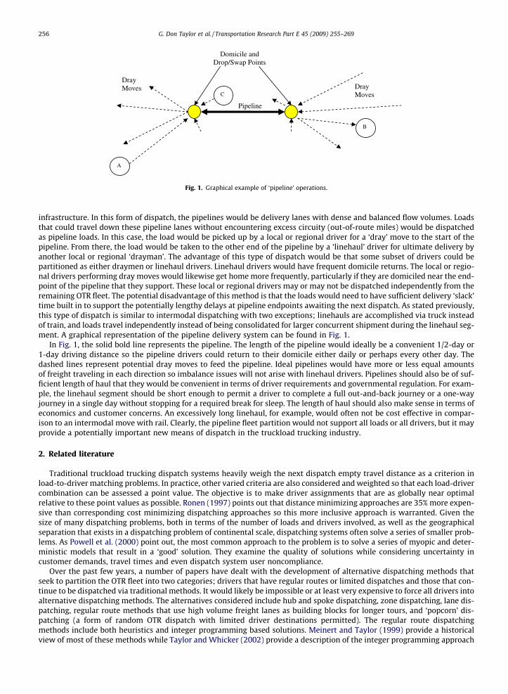
infrastructure. In this form of dispatch, the pipelines would be delivery lanes with dense and balanced flow volumes. Loadsthat could travel down these pipeline lanes without encountering excess circuity (out-of-route miles) would be dispatchedas pipeline loads. In this case, the load would be picked up by a local or regional driver for a ‘dray’ move to the start of thepipeline. From there, the load would be taken to the other end of the pipeline by a ‘linehaul’ driver for ultimate delivery byanother local or regional ‘drayman’. The advantage of this type of dispatch would be that some subset of drivers could bepartitioned as either draymen or linehaul drivers. Linehaul drivers would have frequent domicile returns. The local or regio-nal drivers performing dray moves would likewise get home more frequently, particularly if they are domiciled near the end-point of the pipeline that they support. These local or regional drivers may or may not be dispatched independently from theremaining OTR fleet. The potential disadvantage of this method is that the loads would need to have sufficient delivery ‘slack’time built in to support the potentially lengthy delays at pipeline endpoints awaiting the next dispatch. As stated previously,this type of dispatch is similar to intermodal dispatching with two exceptions; linehauls are accomplished via truck insteadof train, and loads travel independently instead of being consolidated for larger concurrent shipment during the linehaul seg-ment. A graphical representation of the pipeline delivery system can be found in Fig. 1.

In Fig. 1, the solid bold line represents the pipeline. The length of the pipeline would ideally be a convenient 1/2-day or1-day driving distance so the pipeline drivers could return to their domicile either daily or perhaps every other day. Thedashed lines represent potential dray moves to feed the pipeline. Ideal pipelines would have more or less equal amountsof freight traveling in each direction so imbalance issues will not arise with linehaul drivers. Pipelines should also be of suf-ficient length of haul that they would be convenient in terms of driver requirements and governmental regulation. For exam-ple, the linehaul segment should be short enough to permit a driver to complete a full out-and-back journey or a one-wayjourney in a single day without stopping for a required break for sleep. The length of haul should also make sense in terms ofeconomics and customer concerns. An excessively long linehaul, for example, would often not be cost effective in compar-ison to an intermodal move with rail. Clearly, the pipeline fleet partition would not support all loads or all drivers, but it mayprovide a potentially important new means of dispatch in the truckload trucking industry.

2. Related literature

Traditional truckload trucking dispatch systems heavily weigh the next dispatch empty travel distance as a criterion inload-to-driver matching problems. In practice, other varied criteria are also considered and weighted so that each load-drivercombination can be assessed a point value. The objective is to make driver assignments that are as globally near optimalrelative to these point values as possible. Ronen (1997) points out that distance minimizing approaches are 35% more expen-sive than corresponding cost minimizing dispatching approaches so this more inclusive approach is warranted. Given thesize of many dispatching problems, both in terms of the number of loads and drivers involved, as well as the geographicalseparation that exists in a dispatching problem of continental scale, dispatching systems often solve a series of smaller prob-lems. As Powell et al. (2000) point out, the most common approach to the problem is to solve a series of myopic and deter-ministic models that result in a ‘good’ solution. They examine the quality of solutions while considering uncertainty incustomer demands, travel times and even dispatch system user noncompliance.

Over the past few years, a number of papers have dealt with the development of alternative dispatching methods thatseek to partition the OTR fleet into two categories; drivers that have regular routes or limited dispatches and those that con-tinue to be dispatched via traditional methods. It would likely be impossible or at least very expensive to force all drivers intoalternative dispatching methods. The alternatives considered include hub and spoke dispatching, zone dispatching, lane dis-patching, regular route methods that use high volume freight lanes as building blocks for longer tours, and ‘popcorn’ dis-patching (a form of random OTR dispatch with limited driver destinations permitted). The regular route dispatchingmethods include both heuristics and integer programming based solutions. Meinert and Taylor (1999) provide a historicalview of most of these methods while Taylor and Whicker (2002) provide a description of the integer programming approach

G. Don Taylor et al. / Transportation Research Part E 45 (2009) 255–269 257

and present the results of comparing the various methods of dispatch. Liu et al. (2003) provide an excellent example of par-titioned fleets with a mixed truck delivery system utilizing both hub and spoke and direct shipment delivery methods.

Most closely related to the current work is that of ‘lane’ dispatching as presented in Taylor (1998) and Taylor et al. (1999).In these papers, it is demonstrated that performance is closely tied to length of haul, that the best lane candidates are thosewith high volume, and that freight imbalance on the lane can destroy the operational effectiveness of the lane. This infor-mation is used to assist in the development of pipelines in this paper, but two key differences exist between lanes and pipes.Lanes serve only a small service area on each side, and more significantly, only one driver is used for each load. As pointedout in Taylor (1998), when one driver is used in lane dispatching, the effective service area size on each side of the laneshould be restricted to approximately 50 miles. The pipeline dispatching system utilizes three drivers for each pipeline load;the linehaul driver and two draymen. The effective service area size on each end of the pipeline is effectively limited only bythe size of the continent served.

Clearly, effective management of delivery pipelines would require the development of new information systems similarto those used in intermodal transport with truck and rail. Fleischmann et al. (2004) discuss the growing availability of real-time information and how it might be exploited for new routing strategies. Golob and Regan (2002) discuss the usefulness ofvarious sources of traffic information in supporting decisions.

3. Experimental plan, supporting data, and evaluative models

The experiments used in this paper to examine pipeline dispatching methods fall into three broad categories; initialexperimentation to determine the general configuration of desirable lanes, secondary research to find truck-only pipelinesfor practical implementation, and simulation experiments to determine the efficacy of the pipeline dispatching methodswhile concurrently considering the effects of pipeline dispatching on the remaining OTR driving fleet.

3.1. Preliminary experiments – pipelines with full freight set

In an effort to determine whether or not pipeline dispatching is a viable alternative in the truckload trucking industry, wemust first determine where the pipelines should be located. We have set up a simple factorial design to examine this issue.Two factors are considered; the method of ‘seeding’ the solution with potential endpoints and the maximum allowable draylengths permitted.

We learned in Taylor (1998) that effective dispatching lanes should be of appropriate distance such that drivers couldtravel either one-way or round-trip within a single day so they would not be required to sleep on the road. We also learnedthat effective lanes must have high and relatively balanced two-way volume. We use this knowledge to select only a fewhigh volume, balanced pipelines between 200 and 250 miles (half-day drive) and 450–500 miles (full-day drive). Since pipe-line drivers would move only on one pathway, they would be assured of returning home frequently (every day or perhapsevery other day). The next issue is how to ‘seed’ solution alternatives with potential endpoints in the study area of the con-tinental United States. Although no direct help exists in the literature to assist in endpoint selection for pipelines, some re-lated literature provides interesting background information. See, for example, ideas about terminal location for intermodalenvironments in Arnold et al. (2004), domicile terminal location in the less-than-truckload (LTL) industry in Hall (2004), anda discussion of shared freight consolidation terminals in urban areas in Regan and Golob (2005).

Our factorial design uses two methods for seeding the solution with endpoints. First, we utilize major inter-state highwayintersections. The rationale for this is that trucks would need to pass through many of these locations anyway and that theywould therefore not add very much excess circuity if pipeline endpoints were located there. We subjectively identified 96candidate locations in the continental United States. Many more candidate intersections exist, but this set provides coverageof major highway intersections that service large population centers and also provides comprehensive geographical coveragein rural areas.

The second method is to select locations that make sense from a business infrastructure viewpoint. The industrial partnerin this research, J.B. Hunt Transport, Inc. (JBHT) is one of the largest truckload trucking companies in the world. They have agreat deal of infrastructure in place that would make convenient pipeline endpoints. This infrastructure includes mainte-nance terminals and intermodal ramp groups, as well as more ‘conceptual’ infrastructure elements such as pricing ‘hubs’,locations with high-profit outbound rates, and the locations of dedicated fleets supporting large individual customers. Fora direct comparison with the 96 highway intersections, 96 of the JBHT ‘infrastructure’ points were selected as potential end-point locations.

The issue of maximum permissible dray lengths is the second primary experimental parameter in the preliminary exper-iments. If pick-up and delivery drays are greatly restricted in length, they can be handled fully by linehaul drivers and theresult is a delivery lane of the type previously presented in Taylor et al. (1999). With longer drays, they can be handled bylocal or regional drivers domiciled at the pipeline endpoints. This helps to further reap the benefits of driver route regular-ization (by creating a set of regional draymen that have frequent domicile returns). If dray moves can be unlimited in length,more pipeline participation can be obtained. This participation is obtained at the expense of maintaining a large OTR drivingpool because the drays would often be too long for local or regional drivers. The two levels of permissible dray length exam-ined in this paper are 250 miles and infinity. Two hundred and fifty miles is the maximum distance that could be reached if it


is desirable for drivers to return to the pipeline endpoint (likely the driver domicile) daily. Infinite drays are in effect limitedonly by continental boundaries.

Fig. 1 illustrates another issue of experimental interest, load circuity. Loads carried on the pipeline must not exhibit ex-cess circuity (out-of-route miles). The figure indicates that long dray moves (for example, point A to point B in the figure) canbe made when the direction of travel for a given load is in the same general direction as the pipeline. Loads that would re-quire back-tracking to get onto the pipeline require shorter drays because such moves would add to circuity (for example,point C to point B in Fig. 1). For purposes of this study, out-of-route miles are defined as the sum of miles traveled on the drayand pipeline moves minus the direct point-to-point delivery miles. The maximum allowable out-of-route miles for pipelineparticipation are fixed at 50 miles. Loads with more than 50 out-of-route miles are not permitted to travel on the pipeline.There is simply not enough profit margins in individual loads to account for the cost of additional out-of-route miles.

In total, we examine four methods for selecting pipelines. We consider two levels of our two primary experimental fac-tors; the seeding method for pipeline endpoints and the maximum permissible dray length. The four scenarios include:

1. (HIWY/1) Endpoints based on highway intersections with infinite drays.2. (HIWY/250) Endpoints based on highway intersections with 250-mile drays.3. (JBHT/1) Endpoints based on J.B. Hunt infrastructure with infinite drays.4. (JBHT/250) Endpoints based on J.B. Hunt infrastructure with 250-mile drays.

Two computer programs have been written to support this research. The first is a coded heuristic (called Pipe Finder) tofind pipeline locations as described in this section and also in Section 3.2. The second program is a discrete-event systemsimulation model to evaluate the performance of pipelines imbedded into an OTR dispatch and delivery network as de-scribed subsequently in Section 3.3. The Pipe Finder heuristic could be easily implemented in almost any general purposelanguage but a powerful simulation platform is required for the evaluative model. For convenience, both programs have beenwritten in the SIMNET II simulation language which also has general purpose constructs.

The most similar related work is in modeling intermodal networks, especially those related to truck and rail. Some of thiswork advocates the use of traditional network analysis while other research is more simulation based. D’Este (1996) treatsintermodal transit as a sequence of linked events that can take advantage of traditional network models. Rizzoli et al. (2002)provide a simulation model that examines a terminal network connected by rail corridors. In both cases, the resulting net-works are similar to those presented herein, but neither addresses the ‘full’ network that includes a residual OTR fleet thatcannot be fully integrated. In fact, no previous published work was found to directly support a joint intermodal/OTR network.

The program used to find the best pipeline locations first locates all feasible ‘pairs’ of node locations from either the listsof highway intersections or JBHT infrastructure locations that meets the desired pipeline distance criteria. Then, each record,representing point-to-point delivery lanes as described subsequently, is read and considers each of the feasible pipelines todetermine whether or not the lane loads could travel on that pipeline without excessive circuity. After all freight is consid-ered, the pipelines are ranked according to the highest volume of ‘balanced’ miles first. In this case, balanced miles are cal-culated for pipeline candidate A–B as Min(Loads A–B, Loads B–A) � (2 � pipeline length in miles). The highest rankedpipeline and information about its load volume is then written to the results and all freight associated with that pipelineis removed from further consideration (the freight cannot be used to support dispatching on more than one pipeline). Sincewe know that pipeline drivers will return to their domicile frequently, it is our goal to maximize the number of pipeline driv-ers by maximizing the miles driven on the pipelines. Clearly, this ranking system favors longer pipelines. Because the pipe-lines are designed to utilize only that freight that would travel along this general path anyway, and because each pipelineaccounts for only a very small fraction of total freight volume, there is effectively no real capacity issues associated with tak-ing as much freight as possible along the pipelines. As described later, overall driver limits effectively constrain the numberof loads that can be carried.

The process is then repeated to find the second ranked pipeline, etc. This continues until the desired number of pipelinesis found. Based on the observed pipeline freight volumes, a subjective analysis of the data indicates that the desired numberof lanes is likely around 10. Additional lanes start to have diminishing returns in terms of having sufficient freight volume tosupport the ‘timing’ issues associated with matching drivers with freight.

The four preliminary experiments are completed using a single, aggregate annual data set supplied by JBHT. This data setholds freight volume information for a full year. Because it is also desirable to know whether or not the best pipelines remainviable during seasonal variability, the four experimental scenarios are again examined using replicates of 12 one-month datasets instead of a single annual data set. These 12 one-month load density files contain records holding load density informa-tion for more than 10,000 point-to-point delivery lanes between JBHT pricing hubs in the continental United States. Eachrecord provides the latitude and longitude of the origin–destination pair that defines the delivery lane and includes the num-ber of loads that travel in each direction on the lane within the month. The data supporting the preliminary research dis-cussed in this section includes intermodal, OTR truck, and dedicated contract service loads. The research discussed inSection 3.2 excludes intermodal freight. One could argue that drivers operating on the dray portion of intermodal movesshould still be considered, but under normal intermodal operations, this sub-set of drivers would perform the same draywork regardless of whether or not truck only pipelines were utilized.

Because loads that travel on the pipeline will need three separate dispatches, loads with a time-critical designation can-not be considered for pipeline delivery. All time-critical loads have therefore been removed from the data sets ultimately


used for experimentation. The actual delays encountered at the load exchange locations at the ends of pipelines are deter-mined by simulation and quantified by changes to mean load lateness (or earliness). Also, because the computationalrequirements for this study are considerable, lanes with less than 2 loads per month have been eliminated from the datasets. These lanes add computational burden but are unlikely to have a strong effect on the ultimate selection of pipelinelocations.

3.2. Secondary experiments – pipelines with truck-only freight set

The experiments presented in Section 3.1 are of great interest because they utilize a full freight set that includes all loadsin a historical database. This is useful for two reasons. First, because carriers are familiar with current intermodal lanes asso-ciated with their full freight base, examination of pipelines found using full freight sets can provide some measure of vali-dation for the methods used. Secondly, full freight experiments can assist a carrier by finding truck-only alternatives that canbenefit from combined OTR and intermodal freight availability. This might be particularly useful in periods of time in whichrail service may be disrupted. Generally speaking, however, pipelines will likely have their greatest utility in supportingtruck-only freight. For this reason, some of the experiments deemed most promising in the preliminary research are re-peated with truck-only data sets. Because it will be shown that the 250-mile dray scenarios do not perform well, only the(HIWY/1) and (JBHT/1) scenarios are repeated in secondary experimentation. Also, because it will be shown that the pipe-lines appear to be fairly robust in terms of seasonality, only the annual data sets are examined with the truck-only freight set.These scenarios are labeled (HIWY/1/No IM) and (JBHT/1/No IM).

The full annual data set supplied by JBHT is huge, with approximately 1.4 million loads. The truck-only data set includes68.2% of these loads and accounts for 39.3% of the total miles in the full data set.

3.3. Experiments to determine the effects of pipelines on the full driving fleet

Finally, experiments are performed to determine the effects of the pipelines on the remaining OTR fleet. If sufficient loadsare partitioned for pipeline delivery, it may exacerbate the problems normally associated with OTR driving. Particularly, itmay affect the ability of OTR dispatchers to obtain adequate daily driving miles without excessive dwell periods betweenloads and it may exacerbate the problem of getting drivers home in a timely manner. The simulation requires drivers to waituntil they can move loaded. Therefore, the issue is the potential loss of OTR loads to pipelines that could otherwise be usedby OTR drivers to return to their domicile.

A detailed simulation model has been prepared to model and examine a total of 5 scenarios, each using the truck-onlyfreight set:

1. Baseline Scenario: This scenario assumes that all loads are carried by the OTR driving fleet.2. (HIWY-Limited): This scenario makes use of the top 10 pipelines in the (HIWY/1) scenario. The ‘limited’ designation

implies that strict controls are in place regarding how many total drivers can be in the system and how many driverscan be made available for each pipeline linehaul. Pipeline limits are based on the number of balanced miles availableon the pipeline under the assumption that drivers are limited to 500 miles/driver/day. The total number of drivers avail-able for all types of dispatching is also limited.

3. (HIWY-Unlimited): This scenario also makes use of the top 10 pipelines in the (HIWY/1) scenario, but only limits thetotal number of drivers in the system, not the number of pipeline drivers on each pipeline. The number of linehaul driversis determined by actual driver needs as determined on a real-time basis by the simulation model. If one pipeline exhibitsa demand spike, additional drivers can be provided at the expense of other less highly utilized pipelines. This permitsbetter performance in the presence of slight freight seasonality.

4. (JBHT-Limited): This scenario makes use of the top 10 pipelines in the (JBHT/1) scenario with pipeline linehaul driverlimits in place.

5. (JBHT-Unlimited): This scenario makes use of the top 10 pipelines in the (JBHT/1) scenario with no specific pipeline line-haul driver limits.

The simulation model used to evaluate the pipelines is much more complex than the Pipe Finder heuristic. Even so, theauthors have been able to significantly reduce coding time by building upon the simulation code developed, verified and val-idated in Taylor (1998). Because model basics are discussed in that paper, we will focus here only on the changes made to themodel to examine pipelines and will refer the reader to Taylor (1998) for additional detail about the intricacies of the sim-ulation model.

Actually, the model presented in Taylor (1998) also examines a partitioned driving fleet, but with regional fleets andremaining OTR. The required changes for the current research involve replacing the regional dispatch code with pipeline dis-patch code. Instead of identifying whether or not a particular load meets the criteria for regional dispatch, the load is iden-tified as either a pipeline load or an OTR load. If it is to be dispatched as a pipeline load, it is picked up by a drayman from theOTR fleet, carried in a linehaul move by a pipeline driver, and delivered by another OTR drayman. Although the pipeline loca-tions are determined by the Pipe Finder heuristic, the actual assignment of loads to pipelines is accomplished dynamicallywithin the simulation.


The pipeline dispatch and load matching problem is much more complicated than in the original regional model pre-sented in Taylor (1998). The regional model made use of the exact same load/driver matching algorithm used for OTR drivers,but with partitions to identify drivers in the various defined regions. The pipeline dispatch system uses OTR dispatchingmethods for the dray moves, but must also match specific drays with a specific pipeline movement. Ultimately, three differ-ent drivers are used for each load. This means that additional validation and verification are required. Verification of codewas achieved by forcing one or more entities through each line of code and by examining detailed trace reports for each path,entity and attribute. Larger scenarios were then examined to find and eliminate latent errors. Validation was accomplishedby expert industry evaluators from JBHT to ensure that results are reasonable in comparison with previous work and actualresults in related situations.

Initialization of the simulation model involves starting with no drivers in the system. Drivers are then ‘created’ as loadsrequest them until the maximum number of permissible drivers in the system is achieved. Test scenarios reveal that oneweek of simulated operation is sufficient to ‘seed’ the simulation with appropriately dispersed drivers, but a 2-week tran-sient period is used to ensure that steady-state operation is fully achieved and that drivers are truly dispersed as they wouldbe in practice. Statistics are collected for the third week of each simulated month of operation.

A number of summary statistics are collected for all drivers and for OTR drivers and pipeline linehaul drivers indepen-dently. The performance statistics include the following:

DRIVERS: The maximum number of drivers created in each dispatch category during the simulation. Dispatch categoriesinclude over-the-road (OTR) drivers, linehaul (PIPE) drivers by pipeline, and the sum of both of these categories (TOTAL).MILES/DAY: The total miles driven per driver per day, again partitioned according to driver type (OTR, PIPE, AND TOTAL).High values are desirable because this is a key measure of efficiency for the carrier and because driver wages are generallybased on miles driven.EMPTY: The average empty miles per dispatch by driver type.LOADED: The average loaded miles per dispatch by driver type.LATE: The percentage of loads delivered late by driver type.DELETED: The percentage of loads deleted because no drivers were available.

Ideally, the metrics would also include specific measures of tour lengths for individual drivers. However, the dispatchingmethods used in industry to eventually force drivers to their domicile are considered prohibitively complicated for inclusionin the evaluative simulation model. Even so, we do know that pipeline drivers would return to their domicile either daily orevery other day based on their designed lengths of haul. This is far less than typical among OTR drivers. We also know thatOTR drivers performing pipeline drays would return to their domicile far more often than typical OTR drivers, particularly ifthey are domiciled at pipeline endpoints. The greatest concern is that partitioning freight to pipelines might negatively affectthe tour lengths of remaining OTR drivers. With more than 87% of miles remaining in the OTR partition in the most ambitiouspipeline case reported in this paper, however, it is doubtful that the remaining OTR tour lengths would be negatively af-fected. Furthermore, ‘surrogate’ metrics such as miles per driver per day indicate strong performance for the remainingOTR fleet.

The data requirements to support the evaluative simulation model used for the research described in this section are con-siderable. In this case, it is necessary to have historical data for individual loads. Each record in this data describes a specificload in terms of its time of arrival to the system, its pick-up and delivery locations, and its due date. Because the run timesassociated with the pipeline evaluations are so substantial and because the JBHT data sets are so massive (supportingapproximately 6000 OTR drivers), we have taken two steps to reduce computational burden. First, we run only five replica-tions of each scenario. Secondly, we use quarter-sized data sets. As in Taylor et al. (2005), we created 1/4-sized data sets byrandomly deleting 3/4 of the records. The 1/4-sized data sets perform within 1% of full data sets for all metrics examined fortest cases. Therefore, as in Taylor et al. (2005), we cap our experiments at 1500 drivers instead of 6000 and utilize the smallerdata sets. Obviously, this is still a very large problem but the reduction enables each scenario to be run in less than 24 h on aPC platform.

4. Results of experimentation

This section contains the results for all of the experiments outlined in Section 3. We will begin with an overview of pre-liminary research to locate pipelines based on a full freight set and to determine whether or not these pipelines are heavilyaffected by freight seasonality. Secondly, we present the pipelines that result from using data sets with intermodal freightremoved. Finally, we present the results from evaluative simulation experiments to determine the operational efficacy ofboth the pipelines and the remaining OTR fleet.

4.1. Preliminary results – pipelines with full freight set

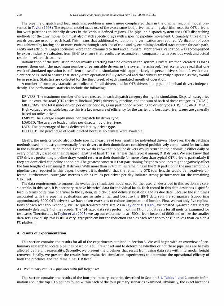
This section contains the results of the four preliminary scenarios described in Section 3.1. Tables 1 and 2 contain infor-mation about the top 10 pipelines found within each of the four primary scenarios examined. Obviously, the exact locations

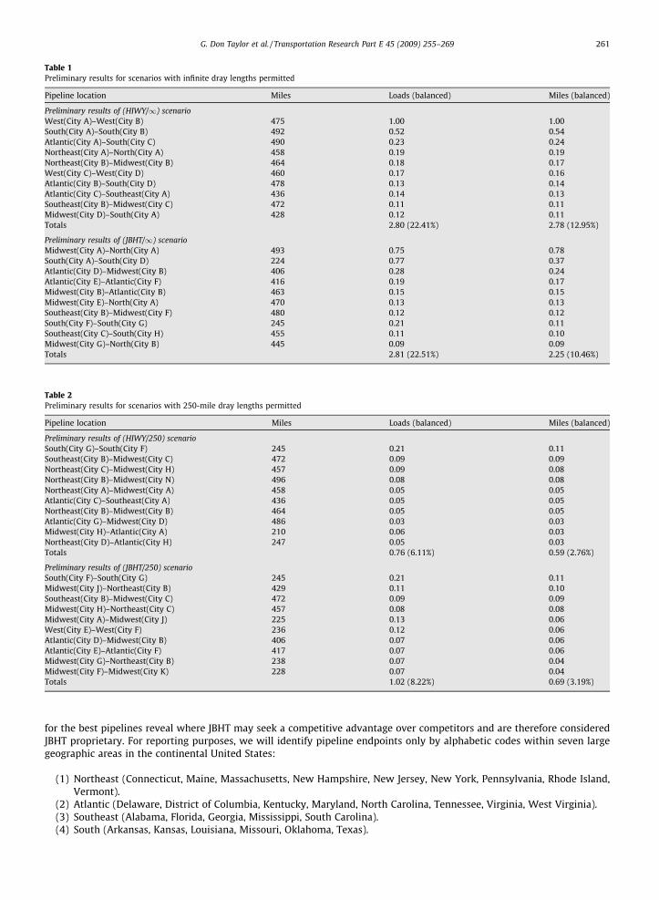
Table 1Preliminary results for scenarios with infinite dray lengths permitted

Pipeline location Miles Loads (balanced) Miles (balanced)

Preliminary results of (HIWY/1) scenarioWest(City A)–West(City B) 475 1.00 1.00South(City A)–South(City B) 492 0.52 0.54Atlantic(City A)–South(City C) 490 0.23 0.24Northeast(City A)–North(City A) 458 0.19 0.19Northeast(City B)–Midwest(City B) 464 0.18 0.17West(City C)–West(City D) 460 0.17 0.16Atlantic(City B)–South(City D) 478 0.13 0.14Atlantic(City C)–Southeast(City A) 436 0.14 0.13Southeast(City B)–Midwest(City C) 472 0.11 0.11Midwest(City D)–South(City A) 428 0.12 0.11Totals 2.80 (22.41%) 2.78 (12.95%)

Preliminary results of (JBHT/1) scenarioMidwest(City A)–North(City A) 493 0.75 0.78South(City A)–South(City D) 224 0.77 0.37Atlantic(City D)–Midwest(City B) 406 0.28 0.24Atlantic(City E)–Atlantic(City F) 416 0.19 0.17Midwest(City B)–Atlantic(City B) 463 0.15 0.15Midwest(City E)–North(City A) 470 0.13 0.13Southeast(City B)–Midwest(City F) 480 0.12 0.12South(City F)–South(City G) 245 0.21 0.11Southeast(City C)–South(City H) 455 0.11 0.10Midwest(City G)–North(City B) 445 0.09 0.09Totals 2.81 (22.51%) 2.25 (10.46%)

Table 2Preliminary results for scenarios with 250-mile dray lengths permitted

Pipeline location Miles Loads (balanced) Miles (balanced)

Preliminary results of (HIWY/250) scenarioSouth(City G)–South(City F) 245 0.21 0.11Southeast(City B)–Midwest(City C) 472 0.09 0.09Northeast(City C)–Midwest(City H) 457 0.09 0.08Northeast(City B)–Midwest(City N) 496 0.08 0.08Northeast(City A)–Midwest(City A) 458 0.05 0.05Atlantic(City C)–Southeast(City A) 436 0.05 0.05Northeast(City B)–Midwest(City B) 464 0.05 0.05Atlantic(City G)–Midwest(City D) 486 0.03 0.03Midwest(City H)–Atlantic(City A) 210 0.06 0.03Northeast(City D)–Atlantic(City H) 247 0.05 0.03Totals 0.76 (6.11%) 0.59 (2.76%)

Preliminary results of (JBHT/250) scenarioSouth(City F)–South(City G) 245 0.21 0.11Midwest(City J)–Northeast(City B) 429 0.11 0.10Southeast(City B)–Midwest(City C) 472 0.09 0.09Midwest(City H)–Northeast(City C) 457 0.08 0.08Midwest(City A)–Midwest(City J) 225 0.13 0.06West(City E)–West(City F) 236 0.12 0.06Atlantic(City D)–Midwest(City B) 406 0.07 0.06Atlantic(City E)–Atlantic(City F) 417 0.07 0.06Midwest(City G)–Northeast(City B) 238 0.07 0.04Midwest(City F)–Midwest(City K) 228 0.07 0.04Totals 1.02 (8.22%) 0.69 (3.19%)


for the best pipelines reveal where JBHT may seek a competitive advantage over competitors and are therefore consideredJBHT proprietary. For reporting purposes, we will identify pipeline endpoints only by alphabetic codes within seven largegeographic areas in the continental United States:

(1) Northeast (Connecticut, Maine, Massachusetts, New Hampshire, New Jersey, New York, Pennsylvania, Rhode Island,Vermont).

(2) Atlantic (Delaware, District of Columbia, Kentucky, Maryland, North Carolina, Tennessee, Virginia, West Virginia).(3) Southeast (Alabama, Florida, Georgia, Mississippi, South Carolina).(4) South (Arkansas, Kansas, Louisiana, Missouri, Oklahoma, Texas).


(5) Midwest (Illinois, Indiana, Michigan, Ohio).(6) North (Iowa, Minnesota, Nebraska, North Dakota, South Dakota, Wisconsin).(7) West (Arizona, California, Colorado, Idaho, Montana, Nevada, New Mexico, Oregon, Utah, Washington, Wyoming).

Note that the number of loads and the number of miles have also been disguised to protect the proprietary nature ofthe results. The scheme used to disguise the findings is to take the ‘best’ pipeline found across all scenarios and to definethe loads and miles for this pipeline both to be ‘1.00’. The pipeline with the largest volume of balanced miles is theWest(City A)-West(City B) corridor in the (HIWY/1) scenario. All other lanes and summary data are then compared tothis best pipeline as a proportion to this value. For example, a lane with 50% of the balanced miles compared to the bestpipeline would have a value of 0.50 in the balanced miles columns in Tables 1 and 2. The same ratio is calculated for thenumber of balanced loads. The last row in the tables includes total values across all 10 pipelines in comparison to thebest pipeline (and the percentage of total balanced miles or loads available in the entire data set). Even though the exactpipeline information is disguised, the approximate locations and adjusted metrics still provide insight into the kinds ofsolutions possible using the techniques described in this paper. The miles shown in the tables are approximate pipelinelengths in miles, calculated as Euclidean distance (adjusted for latitude) between the pipeline endpoints, multiplied by1.17, which is the approximate circuity in North America that is associated with road use instead of straight-linedistance.

Two primary metrics exist to define the quality of the pipeline, the number of two-way balanced loads that travel on thepipeline and the number of loaded and balanced miles on the pipeline. Note that the largest quantity of miles traveled onpipeline segments is in the (HIWY/1) scenario where 12.95% of all miles traveled are on the top ten pipeline linehaul seg-ments. The largest number of loads in any scenario is in the (JBHT/1) scenario. This larger number of loads is brought aboutbecause two of the pipelines based on the JBHT endpoints are in the ½-day range between 200 and 250 miles. It takesroughly twice as many loads to achieve the same number of loaded miles in this situation.

Tables 1 and 2 reveal that much better pipeline participation occurs when infinite drays are permitted. This is, ofcourse, an expected result but the magnitude of the difference is surprising. With drays limited to 250 miles, pipeline par-ticipation is in the range of 2–4% of total loaded miles while participation is in the 10–13% range with infinite drayspermitted.

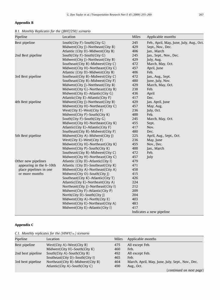
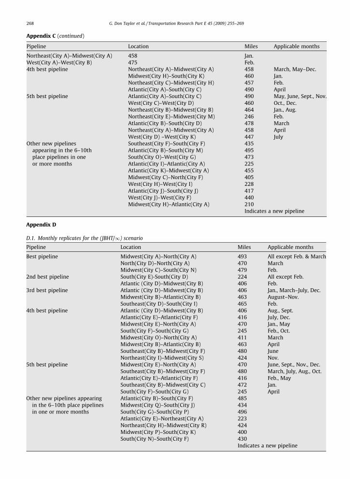
These preliminary experiments were repeated using replicates based on 12 one-month data sets to determine whether ornot the results are seasonal. The results of this experimentation are provided in Appendices A, B, C, D. Surprisingly, thepipelines presented in Tables 1 and 2 are quite robust in terms of being good solutions throughout the year. The most widelyused pipelines in each of the four basic scenarios remain the best pipelines in a majority of months throughout the year. Forexample, West(City A)-West(City B) in Appendix C is still the best (HIWY/1) pipeline 11 months of the year and is the thirdbest pipeline in the remaining month. Similar results are obtained in all four basic scenarios. Also, very few ‘new’ pipelinesappear in the monthly analyses that were not already in the top 10 solution obtained using the single, annual data set. Theseresults tend to indicate robustness in the distribution of freight around the selected pipelines. A review of the appendiceswill provide additional insight for the interested reader.

A review of Tables 1 and 2 indicate that the highway intersections operate best in terms of balanced milesparticipation with infinite drays while JBHT infrastructure endpoints work best with limited drays. Conceptually, this re-sult is intuitive because JBHT infrastructure tends to grow up around local or regional market areas that make sense tothe company. The inter-state highway system grew up in response to the greater transportation needs of the entirecountry.

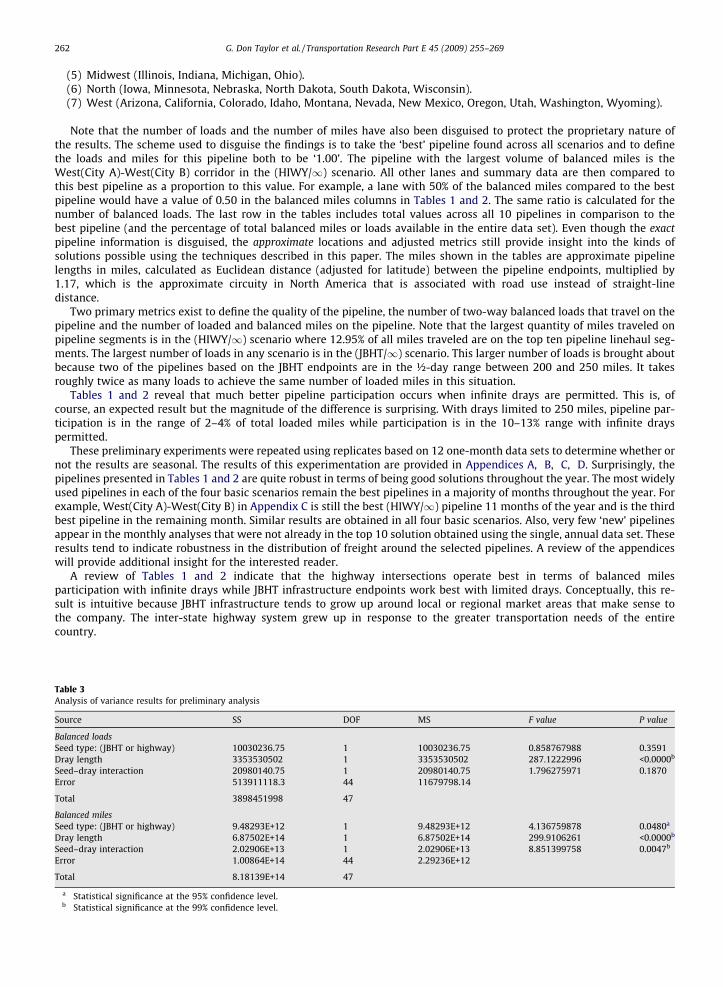
Table 3Analysis of variance results for preliminary analysis

Source SS DOF MS F value P value

Balanced loadsSeed type: (JBHT or highway) 10030236.75 1 10030236.75 0.858767988 0.3591Dray length 3353530502 1 3353530502 287.1222996 <0.0000b

Seed–dray interaction 20980140.75 1 20980140.75 1.796275971 0.1870Error 513911118.3 44 11679798.14

Total 3898451998 47

Balanced milesSeed type: (JBHT or highway) 9.48293E+12 1 9.48293E+12 4.136759878 0.0480a

Dray length 6.87502E+14 1 6.87502E+14 299.9106261 <0.0000b

Seed–dray interaction 2.02906E+13 1 2.02906E+13 8.851399758 0.0047b

Error 1.00864E+14 44 2.29236E+12

Total 8.18139E+14 47

a Statistical significance at the 95% confidence level.b Statistical significance at the 99% confidence level.


After completing the monthly replicates, it is possible to determine whether or not the observed results are statisticallysignificant. To make this determination, analysis of variance (ANOVA) has been completed for the two primary metrics, bal-anced loads and balanced miles. The results of this testing appear in Table 3.

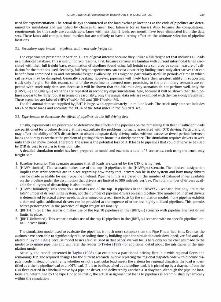
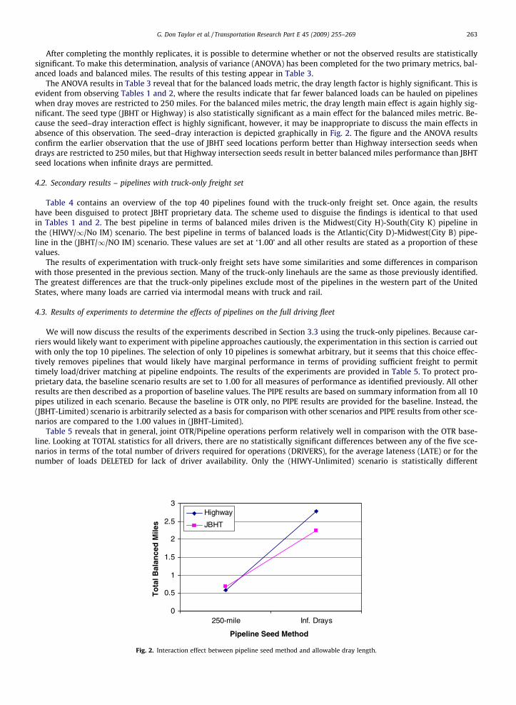
The ANOVA results in Table 3 reveal that for the balanced loads metric, the dray length factor is highly significant. This isevident from observing Tables 1 and 2, where the results indicate that far fewer balanced loads can be hauled on pipelineswhen dray moves are restricted to 250 miles. For the balanced miles metric, the dray length main effect is again highly sig-nificant. The seed type (JBHT or Highway) is also statistically significant as a main effect for the balanced miles metric. Be-cause the seed–dray interaction effect is highly significant, however, it may be inappropriate to discuss the main effects inabsence of this observation. The seed–dray interaction is depicted graphically in Fig. 2. The figure and the ANOVA resultsconfirm the earlier observation that the use of JBHT seed locations perform better than Highway intersection seeds whendrays are restricted to 250 miles, but that Highway intersection seeds result in better balanced miles performance than JBHTseed locations when infinite drays are permitted.

4.2. Secondary results – pipelines with truck-only freight set

Table 4 contains an overview of the top 40 pipelines found with the truck-only freight set. Once again, the resultshave been disguised to protect JBHT proprietary data. The scheme used to disguise the findings is identical to that usedin Tables 1 and 2. The best pipeline in terms of balanced miles driven is the Midwest(City H)-South(City K) pipeline inthe (HIWY/1/No IM) scenario. The best pipeline in terms of balanced loads is the Atlantic(City D)-Midwest(City B) pipe-line in the (JBHT/1/NO IM) scenario. These values are set at ‘1.00’ and all other results are stated as a proportion of thesevalues.

The results of experimentation with truck-only freight sets have some similarities and some differences in comparisonwith those presented in the previous section. Many of the truck-only linehauls are the same as those previously identified.The greatest differences are that the truck-only pipelines exclude most of the pipelines in the western part of the UnitedStates, where many loads are carried via intermodal means with truck and rail.

4.3. Results of experiments to determine the effects of pipelines on the full driving fleet

We will now discuss the results of the experiments described in Section 3.3 using the truck-only pipelines. Because car-riers would likely want to experiment with pipeline approaches cautiously, the experimentation in this section is carried outwith only the top 10 pipelines. The selection of only 10 pipelines is somewhat arbitrary, but it seems that this choice effec-tively removes pipelines that would likely have marginal performance in terms of providing sufficient freight to permittimely load/driver matching at pipeline endpoints. The results of the experiments are provided in Table 5. To protect pro-prietary data, the baseline scenario results are set to 1.00 for all measures of performance as identified previously. All otherresults are then described as a proportion of baseline values. The PIPE results are based on summary information from all 10pipes utilized in each scenario. Because the baseline is OTR only, no PIPE results are provided for the baseline. Instead, the(JBHT-Limited) scenario is arbitrarily selected as a basis for comparison with other scenarios and PIPE results from other sce-narios are compared to the 1.00 values in (JBHT-Limited).

Table 5 reveals that in general, joint OTR/Pipeline operations perform relatively well in comparison with the OTR base-line. Looking at TOTAL statistics for all drivers, there are no statistically significant differences between any of the five sce-narios in terms of the total number of drivers required for operations (DRIVERS), for the average lateness (LATE) or for thenumber of loads DELETED for lack of driver availability. Only the (HIWY-Unlimited) scenario is statistically different

0

0.5

1

1.5

2

2.5

3

250-mile Inf. Drays

Pipeline Seed Method

To

tal B

alan

ced

Mile

s

Highway

JBHT

Fig. 2. Interaction effect between pipeline seed method and allowable dray length.

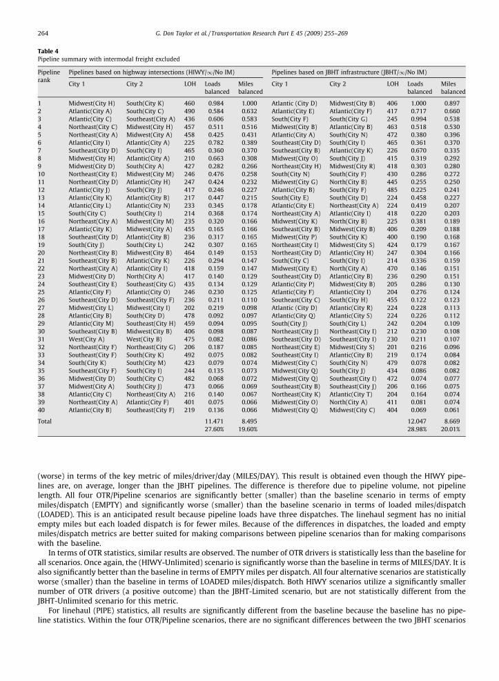
Table 4Pipeline summary with intermodal freight excluded

Pipelinerank

Pipelines based on highway intersections (HIWY/1/No IM) Pipelines based on JBHT infrastructure (JBHT/1/No IM)

City 1 City 2 LOH Loadsbalanced

Milesbalanced

City 1 City 2 LOH Loadsbalanced

Milesbalanced

1 Midwest(City H) South(City K) 460 0.984 1.000 Atlantic (City D) Midwest(City B) 406 1.000 0.8972 Atlantic(City A) South(City C) 490 0.584 0.632 Atlantic(City E) Atlantic(City F) 417 0.717 0.6603 Atlantic(City C) Southeast(City A) 436 0.606 0.583 South(City F) South(City G) 245 0.994 0.5384 Northeast(City C) Midwest(City H) 457 0.511 0.516 Midwest(City B) Atlantic(City B) 463 0.518 0.5305 Northeast(City A) Midwest(City A) 458 0.425 0.431 Atlantic(City A) South(City N) 472 0.380 0.3966 Atlantic(City I) Atlantic(City A) 225 0.782 0.389 Southeast(City D) South(City I) 465 0.361 0.3707 Southeast(City D) South(City I) 465 0.360 0.370 Southeast(City B) Atlantic(City K) 226 0.670 0.3358 Midwest(City H) Atlantic(City A) 210 0.663 0.308 Midwest(City O) South(City J) 415 0.319 0.2929 Midwest(City D) South(City A) 427 0.282 0.266 Northeast(City H) Midwest(City R) 418 0.303 0.28010 Northeast(City E) Midwest(City M) 246 0.476 0.258 South(City N) South(City F) 430 0.286 0.27211 Northeast(City D) Atlantic(City H) 247 0.424 0.232 Midwest(City G) North(City B) 445 0.255 0.25012 Atlantic(City J) South(City J) 417 0.246 0.227 Atlantic(City B) South(City F) 485 0.225 0.24113 Atlantic(City K) Atlantic(City B) 217 0.447 0.215 South(City E) South(City D) 224 0.458 0.22714 Atlantic(City L) Atlantic(City N) 233 0.345 0.178 Atlantic(City E) Northeast(City A) 224 0.419 0.20715 South(City C) South(City I) 214 0.368 0.174 Northeast(City A) Atlantic(City I) 418 0.220 0.20316 Northeast(City A) Midwest(City M) 235 0.320 0.166 Midwest(City K) North(City B) 225 0.381 0.18917 Atlantic(City K) Midwest(City A) 455 0.165 0.166 Southeast(City B) Midwest(City B) 406 0.209 0.18818 Southeast(City D) Atlantic(City B) 236 0.317 0.165 Midwest(City P) South(City K) 400 0.190 0.16819 South(City J) South(City L) 242 0.307 0.165 Northeast(City I) Midwest(City S) 424 0.179 0.16720 Northeast(City B) Midwest(City B) 464 0.149 0.153 Northeast(City D) Atlantic(City H) 247 0.304 0.16621 Southeast(City B) Atlantic(City K) 226 0.294 0.147 South(City C) South(City I) 214 0.336 0.15922 Northeast(City A) Atlantic(City I) 418 0.159 0.147 Midwest(City E) North(City A) 470 0.146 0.15123 Midwest(City D) North(City A) 417 0.140 0.129 Southeast(City D) Atlantic(City B) 236 0.290 0.15124 Southeast(City E) Southeast(City G) 435 0.134 0.129 Atlantic(City P) Midwest(City B) 205 0.286 0.13025 Atlantic(City F) Atlantic(City O) 246 0.230 0.125 Atlantic(City F) Atlantic(City I) 204 0.276 0.12426 Southeast(City D) Southeast(City F) 236 0.211 0.110 Southeast(City C) South(City H) 455 0.122 0.12327 Midwest(City L) Midwest(City I) 202 0.219 0.098 Atlantic (City D) Atlantic(City R) 224 0.228 0.11328 Atlantic(City B) South(City D) 478 0.092 0.097 Atlantic(City Q) Atlantic(City S) 224 0.226 0.11229 Atlantic(City M) Southeast(City H) 459 0.094 0.095 South(City J) South(City L) 242 0.204 0.10930 Southeast(City B) Midwest(City B) 406 0.098 0.087 Northeast(City J) Northeast(City I) 212 0.230 0.10831 West(City A) West(City B) 475 0.082 0.086 Southeast(City D) Southeast(City I) 230 0.211 0.10732 Northeast(City F) Northeast(City G) 206 0.187 0.085 Northeast(City E) Midwest(City S) 201 0.216 0.09633 Southeast(City F) South(City K) 492 0.075 0.082 Southeast(City I) Atlantic(City B) 219 0.174 0.08434 South(City K) South(City M) 423 0.079 0.074 Midwest(City C) South(City N) 479 0.078 0.08235 Southeast(City F) South(City I) 244 0.135 0.073 Midwest(City Q) South(City J) 434 0.086 0.08236 Midwest(City D) South(City C) 482 0.068 0.072 Midwest(City Q) Southeast(City I) 472 0.074 0.07737 Midwest(City A) South(City J) 473 0.066 0.069 Southeast(City B) Southeast(City J) 206 0.166 0.07538 Atlantic(City C) Northeast(City A) 216 0.140 0.067 Northeast(City K) Atlantic(City T) 204 0.164 0.07439 Northeast(City A) Atlantic(City F) 401 0.075 0.066 Midwest(City O) North(City A) 411 0.081 0.07440 Atlantic(City B) Southeast(City F) 219 0.136 0.066 Midwest(City Q) Midwest(City C) 404 0.069 0.061

Total 11.471 8.495 12.047 8.66927.60% 19.60% 28.98% 20.01%


(worse) in terms of the key metric of miles/driver/day (MILES/DAY). This result is obtained even though the HIWY pipe-lines are, on average, longer than the JBHT pipelines. The difference is therefore due to pipeline volume, not pipelinelength. All four OTR/Pipeline scenarios are significantly better (smaller) than the baseline scenario in terms of emptymiles/dispatch (EMPTY) and significantly worse (smaller) than the baseline scenario in terms of loaded miles/dispatch(LOADED). This is an anticipated result because pipeline loads have three dispatches. The linehaul segment has no initialempty miles but each loaded dispatch is for fewer miles. Because of the differences in dispatches, the loaded and emptymiles/dispatch metrics are better suited for making comparisons between pipeline scenarios than for making comparisonswith the baseline.

In terms of OTR statistics, similar results are observed. The number of OTR drivers is statistically less than the baseline forall scenarios. Once again, the (HIWY-Unlimited) scenario is significantly worse than the baseline in terms of MILES/DAY. It isalso significantly better than the baseline in terms of EMPTY miles per dispatch. All four alternative scenarios are statisticallyworse (smaller) than the baseline in terms of LOADED miles/dispatch. Both HIWY scenarios utilize a significantly smallernumber of OTR drivers (a positive outcome) than the JBHT-Limited scenario, but are not statistically different from theJBHT-Unlimited scenario for this metric.

For linehaul (PIPE) statistics, all results are significantly different from the baseline because the baseline has no pipe-line statistics. Within the four OTR/Pipeline scenarios, there are no significant differences between the two JBHT scenarios

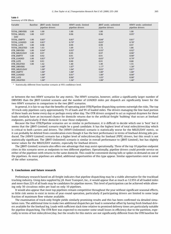
Table 5Summary of OTR Effects

Variable Baseline JBHT seeds; limitedpipeline drivers

HIWY seeds; limitedpipeline drivers

JBHT seeds; unlimitedpipeline drivers

HIWY seeds; unlimitedpipeline drivers

TOTAL_DRIVERS 1.00 1.00 1.00 1.00 1.00TOTAL_MILES/

DAY1.00 0.97 0.96 0.96 0.95a

TOTAL_EMPTY 1.00 0.85a 0.83a 0.84a 0.81a

TOTAL_LOADED 1.00 0.83a 0.79a 0.83a 0.78a

TOTAL_LATE 1.00 0.98 0.99 0.99 0.97TOTAL_DELETED 1.00 1.63 1.69 1.72 1.86OTR_DRIVERS 1.00 0.94a 0.93a 0.93a 0.92a

OTR_MILES/DAY 1.00 0.97 0.95 0.97 0.96a

OTR_EMPTY 1.00 0.92 0.91 0.91 0.90a

OTR_LOADED 1.00 0.83a 0.79a 0.83a 0.79a

OTR_LATE 1.00 0.91 0.90 0.91 0.88OTR_DELETED 1.00 1.42 1.40 1.49 1.55PIPE_DRIVERS 1.00a 1.07a 1.17a 1.30a

PIPE_MILES/DAY 1.00a 1.04a 0.83a 0.87a

PIPE_EMPTY 1.00a 1.00a 1.00a 1.00a

PIPE_LOADED 1.00a 0.91a 1.00a 0.90a

PIPE_LATE 1.00a 0.96a 1.03a 0.98a

PIPE_DELETED 1.00a 1.36a 1.08a 1.46a

a Statistically different from baseline scenario at 95% confidence level.


or between the two HIWY scenarios for any metric. The HIWY scenarios, however, utilize a significantly larger number ofDRIVERS than the JBHT-Limited scenario and the number of LOADED miles per dispatch are significantly lower for thetwo HIWY scenarios in comparison to the two JBHT scenarios.

In general, it is fair to say that the benefits of operating joint OTR/Pipeline dispatching systems outweigh the risks. The top10 truck-only pipelines carry approximately 7% of loads and 9% of loaded miles. The drivers managing the line-haul portionof these loads are home every day or perhaps every other day. The OTR drivers assigned to act as regional draymen for theseloads similarly have an increased chance for domicile returns due to the artificial freight ‘hubbing’ that occurs at linehaulendpoints, particularly if their domicile is near those endpoints.

Because the four OTR/Pipeline scenarios are so similar in performance, it is difficult to decide which one is ‘best’ but itseems that the (JBHT-Limited) scenario might be a good candidate. It has the highest level of total miles/driver/day whichis critical to both carriers and drivers. The (HIWY-Unlimited) scenario is statistically worse for the MILES/DAY metric, soit can probably be deleted from consideration even though it has the best performance in terms of linehaul driving jobs pro-duced. The (HIWY-Limited) scenario has a higher level of miles/driver/day for linehaul (PIPE) drivers, but this result is notstatistically significant. The (JBHT-Unlimited) scenario is similar in overall performance to (JBHT-Limited), but has slightlyworse values for the MILES/DAY statistic, especially for linehaul drivers.

The (JBHT-Limited) scenario also offers one advantage that may assist operationally. Three of the top 10 pipeline endpointcities in this scenario serve as endpoints to two different pipelines. Operationally, pipeline drivers could provide service oneither of the pipelines with returns to the same domicile. This could be convenient during lulls or spikes in demand on one ofthe pipelines. As more pipelines are added, additional opportunities of this type appear. Similar opportunities exist in someof the other scenarios.

5. Conclusions and future research

Preliminary research based on all freight indicates that pipeline dispatching may be a viable alternative for the truckloadtrucking industry. Using data supplied by J.B. Hunt Transport, Inc., it would appear that as much as 12.95% of all loaded milesand more than 22% of all loads may be candidates for pipeline moves. This level of participation can be achieved while allow-ing only 50 circuitous miles per load on only 10 pipelines.

It would also appear that most top pipelines remain competitive throughout the year without significant seasonal effects,so little risk seems to exist in terms of year-round operation, particularly if participating drivers are limited to some largefraction of maximum flow volume available.

The examination of truck-only freight yields similarly promising results and this has been confirmed via detailed simu-lation runs. The additional time to make two additional dispatches per load is somewhat offset by having fresh linehaul driv-ers available for the linehaul leg. Loads with sufficient slack time relative to promised delivery times are particularly suitablefor pipeline dispatching. The OTR fleet was expected to encounter some small losses in efficiency due to the partition, espe-cially in terms of lost miles/driver/day, but the results for this metric are not significantly different from the OTR baseline for


three of the four pipeline scenarios examined. The scenario featuring endpoints based on company infrastructure with strictlinehaul driver limits and with unrestricted dray lengths appears to be the best option in terms of configuration. Thatscenario also offers significant operational opportunities based on having several cities that serve as an endpoint for multiplepipelines. It would also appear that the job of draying loads to/from linehaul endpoints can be accomplished by the OTR fleet.An interesting next step might be to determine whether or not additional gains can be obtained by separating the OTR andpipeline dray fleets. Because this analysis would require significant additional simulation coding and runs, it is left as a futureexercise.

In summary, the research presented herein has raised the possibility that pipeline dispatching is feasible in truckloadtrucking from an operational perspective. Companies would still need to take a rigorous look at related costs for theirparticular situation before establishing the dispatching method. It is unlikely that smaller companies could benefitfrom pipeline dispatching to the extent that a large company like J.B. Hunt Transport, Inc. could benefit because reducingthe available freight from a much smaller freight base might negatively affect a smaller company’s remaining OTRfleet. Finally, it would likely be wise to phase in the use of pipeline dispatching, one pipeline at a time, with a lim-ited number of drivers. In this way, the operational efficacy and cost efficiency can be examined prior to fullimplementation.

Appendix A

A.1. Monthly replicates for the (HIWY/250) scenario

Pipeline Location Miles Applicable months

Best pipeline South(City G)–South(City F) 245 Jan., Feb., April, May, June, July, Aug.,Oct., Dec.

Northeast(City B)–Midwest(City I) 496 Sept., Nov.Southeast(City B)–Midwest(City C) 472 March

2nd best pipeline Northeast(City C)–Midwest(City H) 457 Feb., April, June, JulySoutheast(City B)–Midwest(City C) 472 Jan., May, Aug., Oct.Northeast(City B)–Midwest(City I) 496 March, Dec.South(City G)–South(City F) 245 Sept., Nov.

3rd best pipeline Southeast(City B)–Midwest(City C) 472 Feb., April, June, July, Sept. Nov.Northeast(City B)–Midwest(City I) 496 Jan, Aug., Oct.Northeast(City B)–Midwest(City B) 464 MarchNortheast(City C)–Midwest(City H) 457 MayNortheast(City D)–Midwest(City H) 472 Dec.

4th best pipeline Northeast(City C)–Midwest(City H) 457 Jan., Aug., Sept., Nov.Northeast(City B)–Midwest(City I) 496 Feb., June, July,Northeast(City A)–Midwest(City A) 458 April, May, Oct.South(City G)–South(City F) 245 MarchSoutheast(City B)–Midwest(City C) 472 Dec.

5th best pipeline Atlantic(City C)–Southeast(City A) 436 June, Aug., Sept., Oct., Nov.Northeast(City A)–Midwest(City A) 458 Jan, March, Dec.Midwest(City T)–South(City K) 494 Feb.Northeast(City B)–Midwest(City I) 496 AprilNortheast(City B)–Midwest(City B) 464 MayNortheast(City B)–Atlantic(City F) 462 July

Other new pipelinesappearing in the 6–10thplace pipelines in oneor more months

Atlantic(City C)–Atlantic(City Q) 433Atlantic(City C)–Northeast(City A) 216Atlantic(City K)–Midwest(City A) 455Midwest(City B)–Atlantic(City B) 463North(City D)–South(City J) 204Southeast(City D)–South(City I) 465Southeast(City A)–Midwest(City C) 456Atlantic(City A)–South(City C) 490Midwest(City H)–Southeast(City B) 485Atlantic(City C)–Atlantic(City I) 493Southeast(City B)–Atlantic(City K) 226Northeast(City C)–Midwest(City M) 447

Indicates a new pipeline


Appendix B

B.1. Monthly Replicates for the (JBHT/250) scenario

Pipeline

Pipeline Location

Best pipeline West(CityMidwest(C

2nd best pipeline South(CitySoutheast(

3rd best pipeline NortheastAtlantic(C

Location

Miles Ap

A)–West(City B) 475 Allity H)–South(City K) 460 FebA)–South(City B) 492 All

City D)–South(City I) 465 Feb(City B)–Midwest(City B) 464 Maity A)–South(City C) 490 Au

Miles

plicable m

except Fe.except Fe.rch, Aprilg., Oct.

Applicable months

Best pipeline
South(City F)–South(City G) 245 Feb., April, May, June, July, Aug., Oct. Midwest(City J)–Northeast(City B) 429 Sept., Nov., Dec. Atlantic (City D)–Midwest(City B) 406 Jan., March
2nd Best pipeline
South(City F)–South(City G) 245 Jan., Sept., Nov., Dec. Midwest(City J)–Northeast(City B) 429 July, Aug. Southeast(City B)–Midwest(City C) 472 March, May, Oct. Midwest(City H)–Northeast(City C) 457 April, June Atlantic (City D)–Midwest(City B) 406 Feb.
3rd Best pipeline
Southeast(City B)–Midwest(City C) 472 Jan., Aug., Sept. Southeast(City B)–Midwest(City F) 480 June, July, Nov. Midwest(City J)–Northeast(City B) 429 March, May, Oct. Midwest(City G)–Northeast(City B) 238 Feb. Midwest(City E)–Atlantic(City G) 436 April Atlantic(City E)–Atlantic(City F) 417 Dec.
4th Best pipeline
Midwest(City J)–Northeast(City B) 429 Jan. April, June Midwest(City H)–Northeast(City C) 457 May, Aug. West(City E)–West(City F) 236 July, Oct. Midwest(City P)–South(City K) 400 Feb. South(City F)–South(City G) 245 March, May, Oct. Midwest(City H)–Northeast(City K) 455 Sept. Atlantic(City E)–Atlantic(City F) 417 Nov. Southeast(City B)–Midwest(City F) 480 Dec.
5th Best pipeline
Midwest(City A)–Midwest(City J) 225 April, Aug., Sept., Oct. West(City E)–West(City F) 236 May, June Midwest(City H)–Northeast(City K) 455 Nov., Dec. Midwest(City P)–South(City K) 400 Jan., March Southeast(City B)–Midwest(City C) 472 Feb. Midwest(City H)–Northeast(City C) 457 July

Atlantic (City D)–Atlantic(City I)
479 Atlantic (City D)–Southeast(City K) 471 Midwest(City A)–Northeast(City A) 458 Midwest(City O)–South(City J) 415 Southeast(City K)–Atlantic(City T) 426 Atlantic(City E)–Northeast(City A) 224 Northeast(City J)–Northeast(City I) 212 Midwest(City F)–Atlantic(City P) 209 North(City D)–South(City J) 204 Midwest(City A)–North(City E) 403 Midwest(City E)–Northeast(City A) 483 Midwest(City E)–Atlantic(City I) 417

Appendix C

C.1. Monthly replicates for the (HIWY/1) scenario

onths

b.

b.

, May, June, July, Sept., Nov., Dec.

(continued on next page)

Appendix D

D.1. Monthly replicates for the (JBHT/1) scenario


Best pipeline Midwest(City A)–North(City A) 493 All except Feb. & MarchNorth(City D)–North(City A) 470 MarchMidwest(City C)–South(City N) 479 Feb.

2nd best pipeline South(City E)-South(City D) 224 All except Feb.Atlantic (City D)–Midwest(City B) 406 Feb.

3rd best pipeline Atlantic (City D)–Midwest(City B) 406 Jan., March–July, Dec.Midwest(City B)–Atlantic(City B) 463 August–Nov.Southeast(City D)–South(City I) 465 Feb.

4th best pipeline Atlantic (City D)–Midwest(City B) 406 Aug., Sept.Atlantic(City E)–Atlantic(City F) 416 July, Dec.Midwest(City E)–North(City A) 470 Jan., MaySouth(City F)–South(City G) 245 Feb., Oct.Midwest(City O)–North(City A) 411 MarchMidwest(City B)–Atlantic(City B) 463 AprilSoutheast(City B)–Midwest(City F) 480 JuneNortheast(City I)–Midwest(City S) 424 Nov.

5th best pipeline Midwest(City E)–North(City A) 470 June, Sept., Nov., Dec.Southeast(City B)–Midwest(City F) 480 March, July, Aug., Oct.Atlantic(City E)–Atlantic(City F) 416 Feb., MaySoutheast(City B)–Midwest(City C) 472 Jan.South(City F)–South(City G) 245 April

Other new pipelines appearingin the 6–10th place pipelinesin one or more months

Atlantic(City B)–South(City F) 485Midwest(City Q)–South(City J) 434South(City G)–South(City P) 496Atlantic(City E)–Northeast(City A) 223Northeast(City H)–Midwest(City R) 424Midwest(City P)–South(City K) 400South(City N)–South(City F) 430


Appendix C (continued)


Northeast(City A)–Midwest(City A) 458 Jan.West(City A)–West(City B) 475 Feb.4th best pipeline Northeast(City A)–Midwest(City A) 458 March, May–Dec.

Midwest(City H)–South(City K) 460 Jan.Northeast(City C)–Midwest(City H) 457 Feb.Atlantic(City A)–South(City C) 490 April

5th best pipeline Atlantic(City A)–South(City C) 490 May, June, Sept., Nov.West(City C)–West(City D) 460 Oct., Dec.Northeast(City B)–Midwest(City B) 464 Jan., Aug.Northeast(City E)–Midwest(City M) 246 Feb.Atlantic(City B)–South(City D) 478 MarchNortheast(City A)–Midwest(City A) 458 AprilWest(City D) –West(City K) 447 July


Southeast(City F)–South(City F) 435Atlantic(City B)–South(City M) 495South(City O)–West(City G) 473Atlantic(City I)–Atlantic(City A) 225Atlantic(City K)–Midwest(City A) 455Midwest(City C)–North(City F) 405West(City H)–West(City I) 228Atlantic(City J)–South(City J) 417West(City J)–West(City F) 440Midwest(City H)–Atlantic(City A) 210




References

Arnold, P., Peeters, D., Thomas, I., 2004. Modelling a rail/road intermodal transportation system. Transportation Research Part E: Logistics andTransportation Review 40, 255–270.

D’Este, G., 1996. An event-based approach to modeling intermodal freight systems. International Journal of Physical Distribution and Logistics Management26, 4–15.

Fleischmann, B., Gnutzmann, S., Sandvob, E., 2004. Dynamic vehicle routing based on online traffic information. Transportation Science 38, 420–433.Golob, T.F., Regan, A.C., 2002. The perceived usefulness of different sources of traffic information to trucking operations. Transportation Research Part E:

Logistics and Transportation Review 38, 97–116.Griffin, G., Kalnback, L., Lantz, B., Rodriguez, J., 2000. Driver retention strategy-the role of a career path. Upper Great Plains Transportation Institute – North

Dakota State University, <http://www.ndsu.edu/ndsu/ugpti/DPpdf/DP135.pdf>.Hall, R., 2004. Domicile selection and risk pooling for trucking networks. IIE Transactions 36, 299–305.Liu, J., Li, C., Chan, C., 2003. Mixed truck delivery systems with both hub-and-spoke and direct shipment. Transportation Research Part E: Logistics and

Transportation Review 39, 325–339.Meinert, T.S., Taylor, G.D., 1999. Summary of route regularization alternatives: a historical perspective. Proceedings of the 1999 Industrial Engineering

Research Conference. In: Taylor, G.D., Malstrom, E.M., Watson, J.A., Standley, K.G. (Eds.), on CD-ROM npdffiles n papers n 063. Institute of IndustrialEngineers, Norcross, GA. 4 p.

Min, H., Emam, A., 2003. Developing the profiles of truck drivers for their successful recruitment and retention: A data mining approach. InternationalJournal of Physical Distribution and Logistics Management 33, 149–162.

Powell, W.B., Towns, M.T., Marar, A., 2000. On the value of optimal myopic solutions for dynamic routing and scheduling problems in the presence of usernoncompliance. Transportation Science 34, 67–85.

Regan, A.C., Golob, T.F., 2005. Trucking industry demand for urban shared use freight terminals. Transportation 32, 23–36.Richardson, H.L., 1994. Can we afford the driver shortage? Transportation and Distribution, 30–34.Rizzoli, A.E., Fornara, N., Gambardella, L.M., 2002. A simulation tool for combined rail/road transport in intermodal terminals. Mathematics and Computers

in Simulation 59, 57–71.Ronen, D., 1997. Alternate mode dispatching. Journal of the Operational Research Society 48, 973–977.Sabnani, V.C., Hall, R.W., 2002. Control of vehicle dispatching on a cyclic route serving trucking terminals. Transportation Research Part A: Policy and

Practice 36, 257–276.Schwartz, M., 1992. J.B. Hunt: The long haul to success. University of Arkansas Press, Fayetteville, AR.Taylor,G.D., 1998. Usingagile dedicated fleets to regularize distribution. In: McGinnis, L., Reveliotis, S. (Eds.), Proceedings of the 1998 Industrial Engineering

Research Conference, on CD-ROM npapers n track02 n sa03 n gdtaylor:pdf. Institute of Industrial Engineers, Norcross, GA. 7 p.Taylor, G.D., DuCote, W.G., Whicker, G.L., 2005. Regional fleet design in truckload trucking. Accepted for publication and to appear in Transportation

Research Part E: Logistics and Transportation Review.Taylor, G.D., Meinert, T.S., Killian, R.C., Whicker, G.L., 1999. Development and analysis of efficient delivery lanes and zones in truckload trucking.

Transportation Research: Part E. 35, 191–205.Taylor, G.D., Whicker, G.L., 2002. Optimization and heuristic methods supporting distributed manufacturing. Production Planning and Control 13, 517–528.United States Department of Transportation, Bureau of Transportation Statistics, 2005. http://products.bts.gov/publications/national_transportation_

statistics/2004/html/table_01_02.html.

http://www.ndsu.edu/ndsu/ugpti/DPpdf/DP135.pdf

http://products.bts.gov/publications/national_transportation_statistics/2004/html/table_01_02.html

http://products.bts.gov/publications/national_transportation_statistics/2004/html/table_01_02.html

design and analysis of delivery ‘pipelines’ in truckload trucking

Documents