derivative-extended pod reduced-order modeling for parameter estimation

Copyright © by SIAM. Unauthorized reproduction of this article is prohibited.

SIAM J. SCI. COMPUT. c© 2013 Society for Industrial and Applied MathematicsVol. 35, No. 6, pp. A2696–A2717

DERIVATIVE-EXTENDED POD REDUCED-ORDER MODELINGFOR PARAMETER ESTIMATION∗

A. SCHMIDT† , A. POTSCHKA‡, S. KORKEL† , AND H. G. BOCK†

Abstract. In this article we consider model reduction via proper orthogonal decomposition(POD) and its application to parameter estimation problems constrained by parabolic PDEs. Weuse a first discretize then optimize approach to solve the parameter estimation problem and show thatthe use of derivative information in the reduced-order model is important. We include directionalderivatives directly in the POD snapshot matrix and show that, equivalently to the stationary case,this extension yields a more robust model with respect to changes in the parameters. Moreover,we propose an algorithm that uses derivative-extended POD models together with a Gauss–Newtonmethod. We give an a posteriori error estimate that indicates how far a suboptimal solution obtainedwith the reduced problem deviates from the solution of the high dimensional problem. Finally wepresent numerical examples that showcase the efficiency of the proposed approach.

Key words. proper orthogonal decomposition, parameter estimation, error estimates

AMS subject classifications. 65C20, 65M20, 65M60, 90C90, 93C20

DOI. 10.1137/120896694

1. Introduction. The aim of this article is to present efficient methods to solveparameter estimation problems with PDE constraints. The parameter estimationproblem is given by a least-squares functional

minp∈R

np

1

2

nM∑i=1

(ηi − h(y(p, ti), p)

ςi

)2

=:1

2‖F (p)‖2 ,(1.1)

where y(p, t) : Rnp × [0, T ] �→ L2(Ω) is a Frechet-differentiable mapping, obtained asa solution of the semilinear parabolic PDE

∂

∂ty = DΔy +R(y, p) in [0, T ]× Ω,

(∇y)Tn+ βy = γg(z) in [0, T ]× ∂Ω,y(0, z) = y0(z) for z ∈ Ω

(1.2)

on the domain [0, T ]× Ω ⊂ R × Rl, l ∈ 1, 2, 3, with boundary ∂Ω, constants D,T, β,

γ, g > 0, the outer normal vector n, and a Frechet-differentiable Nemytskii operatorR : L2(Ω) × R

np → L2(Ω). The objective comprises the measurement data vectorη ∈ R

nM , where nM > np and the measurement ηi is taken at time instance ti.

∗Submitted to the journal’s Methods and Algorithms for Scientific Computing section Octo-ber 26, 2012; accepted for publication (in revised form) September 3, 2013; published electronicallyDecember 3, 2013. This work was partially supported by BASF within the junior research groupexperimental design and by the Federal Ministry of Education and Research (BMBF, Germany)within the SBCancer project.

http://www.siam.org/journals/sisc/35-6/89669.html†Interdisciplinary Center for Scientific Computing (IWR), Heidelberg University, Im Neuenheimer

Feld 368, 69120 Heidelberg, Germany ([email protected], [email protected], [email protected]).

‡Interdisciplinary Center for Scientific Computing (IWR), Heidelberg University, Im NeuenheimerFeld 368, 69120 Heidelberg, Germany ([email protected]). This author’s work wassupported by the German Research Foundation (DFG) within the priority program SPP1253 undergrant BO864/12-1.

A2696

Dow

nloa

ded

11/1

5/14

to 1

29.4

9.23

.145

. Red

istr

ibut

ion

subj

ect t

o SI

AM

lice

nse

or c

opyr

ight

; see

http

://w

ww

.sia

m.o

rg/jo

urna

ls/o

jsa.

php


DERIVATIVE-EXTENDED POD FOR PARAMETER ESTIMATION A2697

Moreover, the objective contains the standard deviation ςi of the measurement errorεi and the measurement function h : L2(Ω)×Rnp → R which is a Frechet-differentiableNemytskii operator. For simplicity we assume h to be real valued, however, the resultscan easily be extended to a vector valued h. Assume that p is the unique solution,determined by the laws of nature. Then we have the relations

ηi = h(y(p, ti), p) + εi,

εi ∼ N (0, ς2i ), i = 1, . . . , nM .

The numerical treatment of problems of this type is typically costly, as the dis-cretization of the dynamics results in large systems that must be solved multiple times.A possibility for saving computation time is the use of model reduction techniques,e.g., proper orthogonal decomposition (POD). An overview of reduced-order modelingfor PDE-constrained optimization can be found in [37] and a brief historical surveyon POD is given in [35]. Articles related to POD and its application to parameterestimation are [3, 22, 32, 41].

In derivative-based optimization methods for PDE-constrained problems one usu-ally distinguishes between first discretize then optimize and first optimize then dis-cretize approaches (see [18]). In this article we discretize the PDE dynamics first andthen consider the resulting optimization problem. We show the beneficial properties ofthis strategy and point out explicitly the difficulties that can arise from a naive applica-tion of POD in this case. We propose extensions to POD to overcome these difficulties.

To improve the POD reduced-order model for the use in optimization we includederivatives with respect to the parameters p in the POD snapshot matrix. We call thisapproach derivative-extended POD (DEPOD). The inclusion of directional derivatives(often referred to as sensitivity information) in snapshot matrices can also be foundin [9, 31, 33, 41], however, there the governing PDEs are all stationary. In [17], time-dependent PDEs are considered and sensitivity information is used to improve thePOD basis. In contrast to their approach the enriched basis here satisfies an extendedPOD optimality condition. In [13] adjoint information is used in the reduced basisfor optimal control of the heat equation. The authors in [20] include adjoints in thesnaphot matrix and compare error estimates for suboptimal controls obtained withreduced-order models from different snapshot collections.

Every POD reduced-order model is related to a typically high dimensional modelwhich we also refer to as the high-fidelity (HiFi) model. One can distinguish betweentwo problems concerning the approximation properties of these models. The firstwe call the POD reconstruction problem where we are interested in the error betweensolutions of the reduced-order model and its corresponding HiFi model both evaluatedwith the exact same data and parameters. On the other hand we have the PODprediction problem, where we are interested in the approximation properties of thetwo models for varying parameter configurations. In previous articles that includederivative information in the reduced model, typically the motivation comes from thePOD prediction problem. In [9, 17] it is shown that the approximation quality isimproved with this extension. The extended reduced-order models we present alsoenjoy this property. In the case of ordinary differential equations an a priori estimatefor the POD prediction error is given in [21]. A sensitivity analysis of the reduced-order model with respect to the data from which the model is constructed is carriedout in [35]. In [10, 27, 28] error estimates for POD reconstruction are given.

We compute the derivatives of the dynamics following the principle of internalnumerical differentiation (IND) [4, 5]. It is a technique related to automatic differ-

Dow

nloa

ded

11/1

5/14

to 1

29.4

9.23

.145

. Red

istr

ibut

ion

subj

ect t

o SI

AM

lice

nse

or c

opyr

ight

; see

http

://w

ww

.sia

m.o

rg/jo

urna

ls/o

jsa.

php


A2698 A. SCHMIDT, A. POTSCHKA, S. KORKEL, AND H. G. BOCK

entiation [15] where during the evaluation of the model a particular treatment of theadaptively controlling components is required.

In [20] a priori estimates for optimal control problems are given where the PODbasis is built from snapshots computed at the solution of the optimal control problemon the basis of the HiFi model. The estimates measure the distance between thissolution and a suboptimal solution of the optimal control problem computed with thereduced-order model. The authors in [23, 24, 40] give a posteriori estimates that donot require the basis to be constructed in the HiFi solution. In this article we presentan a posteriori error estimate for parameter estimation problems solved via a Gauss–Newton algorithm under natural assumptions on the problem dynamics. The estimateis based on the local contraction theorem stated in [6]. Moreover, we introduce aDEPOD algorithm which is a variation of the POD optimization algorithms proposedin [1, 19, 36, 41]. Upon convergence of the DEPOD algorithm the a posteriori estimatedelivers the error with respect to the HiFi problem.

Contributions: We discuss the advantages and difficulties that arise with afirst discretize then optimize approach for POD in PDE-constrained optimization.We show how to efficiently include forward derivative information directly in thesnapshot matrix of POD in the case of time-dependent problems. Moreover, we givean a posteriori error estimate for a Gauss–Newton algorithm based on a local contrac-tion theorem. This estimate is an indicator for the quality of a suboptimal solutionobtained from the DEPOD algorithm we propose.

Outline: We recall the computation of a POD basis and how this basis is usedto construct a reduced-order model in sections 2 and 3. Then we describe a generaland efficient method to compute derivatives for time-dependent models in section 4.This derivative information is used in the POD basis construction in section 5 and wediscuss the properties of the enriched model. In section 6 we propose an algorithmto solve the parameter estimation problem based on a Gauss–Newton method. Sec-tion 7 contains the main theoretical convergence results and an error estimate and insection 8 we present numerical examples that confirm the theoretical results.

2. Proper orthogonal decomposition (POD). In this section we briefly de-scribe the basic method for obtaining a reduced basis from a given number of datavectors via POD. A more detailed introduction to POD can be found in the surveyof Kunisch and Volkwein [26]. We work in the time-discrete setting of POD, whichmeans that we apply POD to a finite set of given vectors αj ∈ R

N , the so-calledsnapshots, taken at different time instances tj . The result of the decomposition willbe a small set of vectors (the POD basis) that can be used to represent the typicallylarge set of given snapshot data vectors αj sufficiently well.

Throughout this article, (·, ·)Ω denotes the L2-inner product on the domain Ω,‖·‖Ω the corresponding norm, (·, ·) the Euclidean scalar product, and ‖·‖ the Euclideannorm. The entries of the dynamic state vectors α(t) are assumed to be the coefficientsof a Galerkin approach for discretization of a time-dependent PDE with an ansatzy(t, z; p) =

∑Ni=1 αi(t; p)ϕi(z), (t, z) ∈ [0, T ] × Ω and V := span{ϕ1(z), . . . , ϕN (z)}.

For simplicity of notation we use the abbreviations yj for y(tj , z; p) and αj for [α1(tj ; p),

. . . , αN (tj ; p)]T .

Assume that from the solution of a time-dependent PDE we have ns snapshotsyj at time instances tj , j = 1, . . . , ns, equidistantly distributed on the time interval[0, T ]. We consider the matrix

A := [α1, . . . , αns ] ∈ RN×ns

Dow

nloa

ded

11/1

5/14

to 1

29.4

9.23

.145

. Red

istr

ibut

ion

subj

ect t

o SI

AM

lice

nse

or c

opyr

ight

; see

http

://w

ww

.sia

m.o

rg/jo

urna

ls/o

jsa.

php



and denote its column rank by d. We call {ψ1(z), . . . , ψk(z)} a POD basis of orderk ≤ d if for every k, it can be obtained as a solution of the optimization problem

minψ1,...,ψk

1

ns

ns∑i=1

∥∥∥∥∥∥yi −k∑j=1

(yi, ψj)Ωψj

∥∥∥∥∥∥2

Ω

s.t. (ψl, ψm)Ω = δlm, 1 ≤ l,m ≤ k.(2.1)

An equivalent characterization of the POD basis is given by the maximizationproblem (see also [26])

maxψ1,...,ψk

1

ns

ns∑i=1

k∑j=1

(yi, ψj)2Ω s.t. (ψl, ψm)Ω = δlm, 1 ≤ l,m ≤ k.

Applying the Lagrange formalism to this problem results in the eigenvalue problem

1

nsAATMuj = σ2

juj ,(2.2)

where M is the symmetric and positive-definite mass matrix with entries Mij =(ϕi, ϕj)Ω. As we have

(ψi, ψj)Ω = (ui,Muj) = δij , 1 ≤ i, j ≤ d,we can transform the eigenvalue problem to obtain orthonormality in the Euclideanspace such that we can apply standard solution methods. By multiplying (2.2) fromthe left with the positive square rootM1/2 ofM (defined as M = (M1/2)TM1/2) andsetting uj =M1/2uj and A =

√1/nsM

1/2A we obtain

AAT uj = σ2j u

j.

The eigenvectors uj ∈ RN are the coefficients of the new basis functions which we also

refer to as POD modes ψj(z) =∑N

i=1 ujiϕi(z). The modified problem can be solved

by singular value decomposition of AA = UΣWT ,

with matrices U ∈ RN×d and W ∈ R

ns×d that have orthonormal columns and adiagonal matrix Σ with singular values σ1 ≥ · · · ≥ σd ≥ 0. By defining Uk :=[U.1, . . . , U.k] the POD coefficient matrix is given by

Ψ := (M1/2)−1Uk ∈ RN×k.

With this matrix the POD modes can be represented as

ψj(z) =

N∑i=1

Ψijϕi(z), j = 1, . . . , k.

We are only interested in the first k eigenvectors of (2.2) corresponding to the k largestsingular values. The residual of the optimization problem (2.1) is given by the PODprojection error formula

1

ns

ns∑i=1

∥∥∥∥∥∥yi −k∑j=1

(yi, ψj)Ωψj

∥∥∥∥∥∥2

Ω

=

d∑i=k+1

σ2i .(2.3)

Dow

nloa

ded

11/1

5/14

to 1

29.4

9.23

.145

. Red

istr

ibut

ion

subj

ect t

o SI

AM

lice

nse

or c

opyr

ight

; see

http

://w

ww

.sia

m.o

rg/jo

urna

ls/o

jsa.

php



Hence, if the singular values decay rapidly, already for small k we have∑di=k+1 σ

2i

� 1 and only a small number k of POD modes is necessary to capture most of theinformation given by the snapshots y1, . . . , yns . For the actual choice of k we considerthe ratio between the modeled and the total energy which is given by

E(k) =∑k

i=1 σ2i∑d

i=1 σ2i

≥ 1− ETOL,(2.4)

where ETOL > 0 (see also [26]). Moreover, in addition to the factor 1/ns a scaling ofthe snapshot sample should be considered. We will discuss this topic in section 5.

Remark 2.1. The POD modes ψj(z) form a basis. We denote the POD subspace

as V := span{ψ1(z), . . . , ψk(z)}. If we choose k = d we have

V = span{y1, . . . , yns}.

3. POD reduced-order modeling. We consider again problem (1.2) for whichwe build a POD reduced-order model. For existence and uniqueness of a solution to(1.2) we refer the reader to [39]. Moreover, we require the solutions to be sufficientlyregular (see [27]). With the Hilbert space V := H1(Ω) we can state the weak form ofthe parabolic PDE (1.2) as

∂

∂t(y, v)Ω = −D(∇y,∇v)Ω +D(γg − βy, v)∂Ω + (R(y, p), v)Ω ∀v ∈ V,

(y(0, z), v)Ω = (y0, v)Ω ∀v ∈ V,(3.1)

where we assume y0 ∈ V . Note that the boundary conditions are imposed weakly.This equation is discretized with a Galerkin method.

With y(t, z; p) =∑N

i=1 αi(t; p)ϕi(z) and v = ϕi(z), i = 1, . . . , N in (3.1), whereϕ1, . . . , ϕN are basis functions of V ⊂ V , we obtain the N -dimensional HiFi model

Mα(t; p) = f(α(t; p), p), α(0; p) = α0, t ∈ [0, T ](3.2)

with mass matrix M as in section 2 and α := dα/dt. Equation (3.2) is called theHiFi model as we assume that the chosen discretization is able to capture the physicalbehavior of the underlying problem (1.2). Moreover,N is typically large. System (3.2)can be integrated using a time-stepping method, for example, the implicit Euler, theCrank–Nicholson scheme, or the backward differentiation formula method.

To build the reduced model we take snapshots yj , i = 1, . . . , ns, obtained viaintegration of (3.2). We then compute the matrix Ψ and POD modes ψj(z), j =

1, . . . , k. With a Galerkin discretization of (3.1), y(t, z; p) :=∑k

i=1 αi(t; p)ψi(z), andsetting v = ψi(z), i = 1, . . . , k, we obtain the POD reduced-order model (POD ROM)

˙α(t; p) = ΨT f(Ψα(t; p), p), α(0; p) = ΨTMα0, t ∈ [0, T ](3.3)

of dimension k � N . By construction the POD space V = span{ψ1(z), . . . , ψk(z)}is a subspace of the Galerkin ansatz space V = span{ϕ1(z), . . . , ϕN (z)}. We cansee that the procedure can also be interpreted as a projection of V on V which isobtained by setting α = Ψα and multiplying (3.2) from the left by ΨT . Note thatthis is possible, as we impose the boundary conditions weakly. In this paper weevaluate the nonlinearities in the POD ROM at the same points in space as for theHiFi model. For practical applications one might consider methods like the discrete

Dow

nloa

ded

11/1

5/14

to 1

29.4

9.23

.145

. Red

istr

ibut

ion

subj

ect t

o SI

AM

lice

nse

or c

opyr

ight

; see

http

://w

ww

.sia

m.o

rg/jo

urna

ls/o

jsa.

php



empirical interpolation method [11] to reduce the number of evaluation points of thenonlinear part.

The reduced model can be used for instance in an optimization algorithm wheremultiple evaluations of the model are necessary. A first concern is the POD recon-struction error defined as

REPOD(t) :=‖y(t, z; p)− y(t, z; p)‖Ω

‖y(t, z)‖Ω,(3.4)

where y and y are solutions of the HiFi model and POD ROM at time t, respectively,computed with the exact same data at p where the basis is constructed. In [27] a priorierror estimates for the POD reconstruction error are given for linear and semilinearparabolic PDEs. For the semilinear problem (3.1) we want to summarize their mainresults in the following remark (for details, see [27, 28]).

Remark 3.1. Assume that for a fixed p we have a nonlinear term R(y, p) thatis locally Lipschitz continuous in y and there is a unique and sufficiently regularsolution to (3.1). Moreover, consider an implicit Euler scheme with ns− 1 time stepsand sufficiently small step size τ := 1/(ns − 1) that allows a stable integration of(3.2) and (3.3). If snapshots are taken at every time instance we obtain the followingestimate (see [27, Theorem 10])

1

ns

ns∑i=1

‖y(ti, z; p)− y(ti, z; p)‖2Ω ≤(C1 + C2ns +

C3

τ2

) d∑i=k+1

σ2i + C4τ

2(3.5)

with constants C1, C2, C3, and C4 independent of k and ns. For k = d the estimatebecomes (see also Remark 2.1)

1

ns

ns∑i=1

‖y(ti, z; p)− y(ti, z; p)‖2Ω ≤ C4τ2.

Hence, the reconstruction error REPOD(t) can be driven to zero by controlling thenumber of POD basis functions and the step size of the implicit Euler scheme.

Remark 3.2. We give here a slightly altered form of the estimate in [27, Theo-rem 10]. As described in [27], the term for the projection error of the initial value in

the estimate can be replaced by C2ns∑d

i=k+1 σ2i . The additional term C3

τ2

∑di=k+1 σ

2i

accounts for the fact that, in contrast to [27], we do not include difference quotients(y(ti, z; p)− y(ti−1, z; p))/τ in the snapshot matrix (compare also [28, Theorem 4.7]).In numerical computations, these additional snapshots yielded significant improve-ments only for very coarse time grids.

Remark 3.3. Note that estimate (3.5) still holds when additional information isincluded in the snapshot matrix used for the basis construction. The proof of theestimate is based on the POD projection formula (2.3) (see [27, Lemma 3]). With anextended snapshots matrix we have instead

1

mns

⎛⎜⎝ ns∑i=1

∥∥∥∥∥∥yi −k∑j=1

(yi, ψj)Ωψj

∥∥∥∥∥∥2

Ω

+

ns(m−1)∑i=1

∥∥∥∥∥∥ρi −k∑j=1

(ρi, ψj)Ωψj

∥∥∥∥∥∥2

Ω

⎞⎟⎠ =

d∑i=k+1

σ2i ,

where ρi ∈ V are additional snapshots used to compute an extended POD basisψj , j = 1, . . . , k, and singular values σi, i = 1, . . . , d. The projection error of the

Dow

nloa

ded

11/1

5/14

to 1

29.4

9.23

.145

. Red

istr

ibut

ion

subj

ect t

o SI

AM

lice

nse

or c

opyr

ight

; see

http

://w

ww

.sia

m.o

rg/jo

urna

ls/o

jsa.

php



original states can then be estimated as

1

ns

ns∑i=1

∥∥∥∥∥∥yi −k∑j=1

(yi, ψj)Ωψj

∥∥∥∥∥∥2

Ω

≤ md∑

i=k+1

σ2i .

Using the inequality instead of (2.3) only alters the constants Cl, l = 1, . . . , 4, in (3.5)and the singular values σi are replaced by σi.

However, in the context of parameter estimation or optimal control we are moreinterested in the use of the POD ROM for POD prediction. By this we mean thatwe evaluate the reduced model to give approximations to the HiFi model for vary-ing parameter configurations p. With changing parameters the POD subspace Vmay be unable to reflect the dynamics of the underlying physical model. This canresult in POD ROM solutions that are bad approximations to the HiFi solutions.To overcome this problem in the optimization context, several improvements havebeen suggested. The authors in [1] use an adaptive strategy, where after finding asuboptimal solution with the reduced-order model, the HiFi model is reevaluated tocreate new snapshots that are added to the matrix A and the POD ROM is rebuilt.In [2, 14] a trust-region method is presented to account for the changing optimiza-tion variables. In [29] the reduced-order optimality system for the control problem isextended which yields a correction of the iteration step proposed with the reduced-order model. A related goal oriented approach to construct the POD basis was takenin [8].

Another approach to generate a more robust ROM is the inclusion of derivativeinformation in the reduced-order model. For stationary problems this has been donefor example in [9, 31]. The ideas are related to the concepts proposed in this articleand will be discussed more thoroughly in the following.

4. Variational differential equations and the principle of IND. As we areworking in a first discretize then optimize setting, the optimization algorithm we userequires the derivative of the objective function only with respect to a finite vectorof optimization variables. In particular we need to compute derivatives of dynamicmodels of type (3.2) and (3.3). In this section we show how this is done efficiently.

We call (3.2) and (3.3) the nominal problems. The solution of these dynamicproblems is obtained by integration in time preferably with a method that includesadaptive components like step size and order control. A straightforward approachis to consider the time-stepping algorithm as black box and use finite differencesor automatic differentiation [15] to approximate the derivatives ∂α(t; p)/∂p. This iscalled external numerical differentiation (END) as opposed to the concept of IND [4, 5,38]. One drawback of END is that it does not take advantage of the internal structuresthat can be exploited during the integration process and, thus, might be inefficient.In the case of finite differences, to obtain proper accuracies of the derivatives at leastnp highly accurate solutions of the dynamical system are necessary, which we usuallycannot afford for PDEs. We consider another approach to obtain this sensitivityinformation.

To a given nominal problem, e.g., the HiFi model (3.2), we can define the varia-tional differential equation (VDE)

Mw =∂f(α, p)

∂αw +

∂f(α, p)

∂p, w(0; p) = 0, w(t; p) :=

∂α(t; p)

∂p∈ R

N×np(4.1)

Dow

nloa

ded

11/1

5/14

to 1

29.4

9.23

.145

. Red

istr

ibut

ion

subj

ect t

o SI

AM

lice

nse

or c

opyr

ight

; see

http

://w

ww

.sia

m.o

rg/jo

urna

ls/o

jsa.

php



that is obtained by differentiation of the nominal problem with respect to the pa-rameter vector p. The VDE is often also called the tangent equation. When solvingthe extended ODE system consisting of (3.2) and (4.1) numerically we need to ex-ploit internal structures for efficiency and require the solutions w(t; p) to be accuratederivatives of (3.2) and consistent with (4.1). This is guaranteed by applying theprinciple of IND.

(1) For the integration the same discretization scheme should be applied to thenominal problem and the VDE. All adaptive components should be fixed.

(2) If matrix decompositions are used for the solutions of the linear subproblems,these should be reused, as the Jacobians of the right-hand sides of the nominalproblem and the VDE are the same.

(3) The choice of the adaptive components should be oriented toward the stabilityneeds of the nominal problem and the VDE simultaneously.

(4) A linear time discretization scheme should be applied.The IND principle can be interpreted from two different viewpoints. On the

one hand, it is an application of automatic differentiation [15] to the integrationscheme, where the dependence of the adaptively chosen components with respectto the parameters is neglected. Hence, assuming that numerically exact derivativesof the right-hand side f are provided (e.g., via automatic differentiation) we obtainnumerically exact derivatives of a fixed discretization scheme. The high accuracy isimportant to obtain descent directions for optimization on the discrete level. On theother hand, as the time integration is a linear discretization, with IND we have aconsistent and stable integration scheme for the VDE. Hence, the discrete computedderivatives are consistent with the continuous problem (4.1). Moreover, note thatby reusing the Jacobians and their decompositions, IND is numerically more efficientthan END, where the integration is considered black box.

5. Derivative-extended proper orthogonal decomposition. When solvingthe parameter estimation problem (1.1) we have to provide directional derivatives ofthe form (∂y(t, p)/∂p)Δp with Δp ∈ R

np . As for the nominal problem we assumethat these derivatives are sufficiently well approximated by solutions of the HiFi VDEgiven as

∂y(t, z; p)

∂pΔp =

N∑i=1

wi(t; p)Δpϕi(z) ∈ V .

Accordingly, a POD ROM approximation of the directional derivative is given by

∂y(t, z; p)

∂pΔp =

k∑i=1

wi(t; p)Δpψi(z) ∈ V ,

where w(t; p) is the solution of the VDE to the POD ROM nominal problem (3.3).Obviously, this approximation is in the same space V as the nominal solutions. How-ever, for the space V we cannot assume that it is able to reflect the dynamic propertiesof the VDE to the HiFi (3.2), as it is purely constructed from snapshots of the nominalsolution. Hence, the POD derivative (∂y(t, z; p)/∂p)Δpmight be a bad approximationof the HiFi derivative (∂y(t, z; p)/∂p)Δp even for POD reconstruction.

This can cause severe problems in derivative-based optimization methods, becausethe optimality conditions depend on derivative information. Furthermore, this canalso be a drawback for optimal control problems like experimental design (see [25]),where the objective contains sensitivity information.

Dow

nloa

ded

11/1

5/14

to 1

29.4

9.23

.145

. Red

istr

ibut

ion

subj

ect t

o SI

AM

lice

nse

or c

opyr

ight

; see

http

://w

ww

.sia

m.o

rg/jo

urna

ls/o

jsa.

php



Remark 5.1. Note that the IND derivatives are numerically exact derivatives toits nominal solution, when a fixed integration scheme and numerically exact deriva-tives of the right-hand sides are used. The IND derivatives of a standard POD ROMin general, however, do not reflect the underlying physical sensitivities.

Remark 5.2. The problem described is inherent to the first discretize then opti-mize approach as the relation between the infinite dimensional counterparts and thediscretely computed derivatives (e.g., via finite differences, automatic differentiation,IND) is unclear. In an indirect approach, however, one can explicitly derive the in-finite dimensional optimality conditions and will typically use a different POD basisfor the nominal equation and the sensitivity equations (either variational differentialequations or the adjoint equation).

We overcome this problem by including the derivative information obtained fromthe HiFi model in the POD reduced-order model. We call this derivative-extendedproper orthogonal decomposition (DEPOD). More precisely it means that we compute

y(tj , z; p) =

N∑i=1

αi(tj ; p)ϕi(z) and∂y(tj , z; p)

∂pel =

N∑i=1

∂αi(tj ; p)

∂pelϕi(z),

j = 1, . . . , ns, l = 1, . . . , np,

with the HiFi model (3.2), where el is the lth column of the np × np identity matrix.We use the coefficients to compose the snapshot matrix

A :=

[ζ0α

1, . . . , ζ0αns , ζ1

∂α

∂p

1

e1, . . . , ζnp

∂α

∂p

ns

enp

]∈ R

N×(ns+ns·np),

where we introduce the weights ζ0, . . . , ζnp belonging to the sets of nominal snapshotsand derivative snapshots for each parameter. It is important to choose these weightscarefully, as different magnitudes in the derivatives and the nominal solutions candeteriorate the quality of the POD basis. By considering the POD optimality condi-tion (2.1) it becomes clear that the magnitude of the singular values corresponds tothe magnitude of the snapshots. Hence, when choosing a certain k, modes belongingto smaller singular values are thrown out and the corresponding information is notcaptured. For the DEPOD basis, we propose to divide by the mean of the L2-normsof the snapshots, i.e.,

ζ0 =ns∑ns

j=1 ‖y(tj , z; p)‖Ω, ζl =

θ · ns∑ns

j=1

∥∥∥∂y(tj ,z;p)∂p el

∥∥∥Ω

, l = 1, . . . , np.

We use the factor θ < 1 (e.g., θ = 0.5) to account for the fact that the derivativesdepend on y(t, z; p) and, thus, the nominal solution should be given more importancein the POD approximation. Note that one can also use weights on each individualsnapshot, which we do not do as later in the parameter estimation we only considerabsolute measurement errors.

We can apply proper orthogonal decomposition to the matrix A in the sameway as presented in section 2. The new POD basis functions now generate a k-dimensional enriched space V = span{ψ1, . . . , ψk} that also contains the dynamicsof the sensitivities. Moreover, ψ1, . . . , ψk obviously satisfy the following extended

Dow

nloa

ded

11/1

5/14

to 1

29.4

9.23

.145

. Red

istr

ibut

ion

subj

ect t

o SI

AM

lice

nse

or c

opyr

ight

; see

http

://w

ww

.sia

m.o

rg/jo

urna

ls/o

jsa.

php



optimality criterion (compare to (2.1))

minψ1,...,ψk

1

(np+1)ns

(ns∑i=1

∥∥∥∥∥∥ζ0(yi −

k∑j=1

(yi, ψj)Ωψj

)∥∥∥∥∥∥2

Ω

+

ns∑i=1

np∑l=1

∥∥∥∥∥∥ζl(∂yi

∂pel −

k∑j=1

(∂yi

∂pel, ψj

)Ω

ψj

)∥∥∥∥∥∥2

Ω

)

s.t. (ψn, ψm)Ω = δnm, 1 ≤ n,m ≤ k.

(5.1)

The number k of modes in the DEPOD basis will most likely be larger than withstandard POD, but one should note that it is still an optimal choice in the sense of(5.1). We choose k again according to the energy quotient (2.4). Thus, togetherwith the weighting of the snapshots we guarantee that the addition of derivativeinformation does not come at the cost of a loss of dynamic information of the nominalproblem (see also Remark 3.3).

A drawback of this approach could be the possibly large number of snapshots thathave to be dealt with in the decomposition. When this becomes an issue, methodsfor optimal snapshot location should be considered (see [30]), such that the essentialdynamics can be captured with fewer samples.

In the following we discuss the POD reconstruction properties of the derivatives.To this end, we first introduce the continuous problem that describes the parametersensitivities (

∂

∂typ, v

)Ω

= −D (∇yp,∇v)Ω +D (−βyp, v)∂Ω

+

(∂

∂yR(y, p)yp +

∂

∂pR(y, p), v

)Ω

∀v ∈ V,

(yp(0, z), v)Ω = (0, v)Ω ∀v ∈ V,

(5.2)

which we can obtain by differentiation of the weak form of the nominal problem(3.1) with respect to p under the given differentiability assumptions. Note that incontrast to (3.1), (5.2) is now linear in yp and we obtain a system of np equations.Throughout this article, we assume that there exist sufficiently regular solutions to(5.2). The differentiated weak form is never used in our practical approach. However,the discrete IND derivatives are related to (5.2). We now show that using a DEPODbasis together with the presented method of derivative computation is essentially anapplication of POD model reduction to the infinite dimensional parameter sensitivityequations.

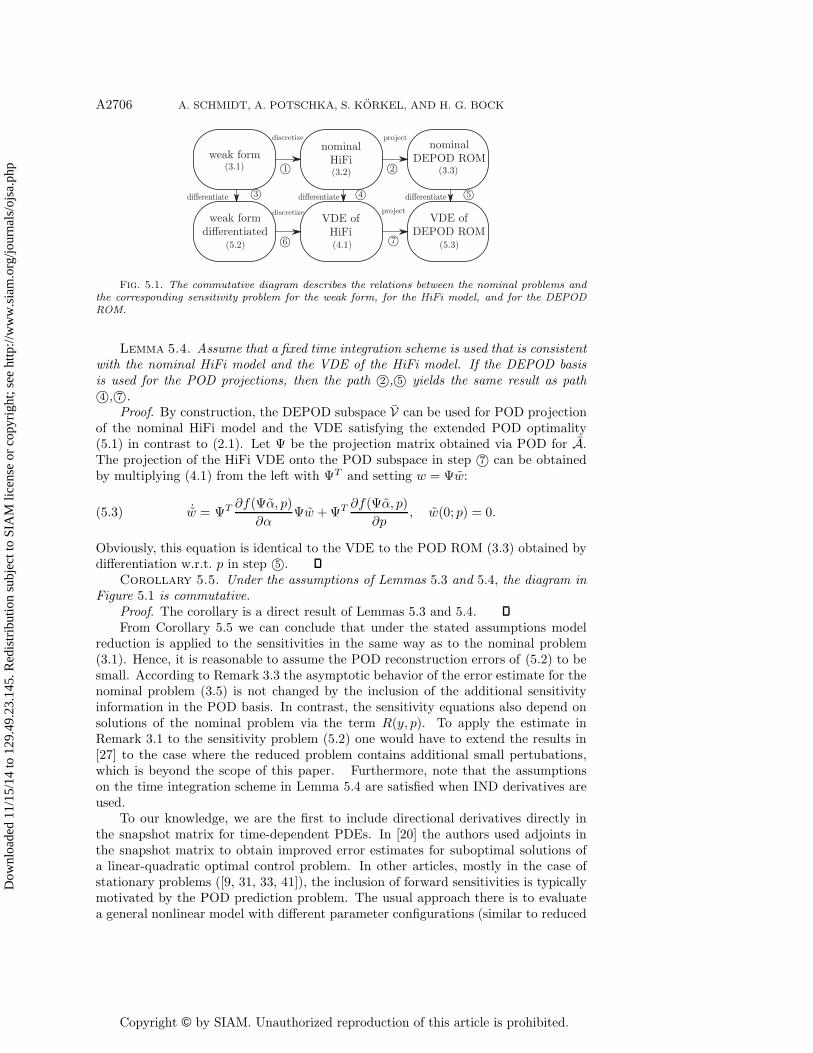
In Figure 5.1 the relations between the nominal problems (3.1), (3.2), and (3.3)and their corresponding sensitivity problems are displayed. By “discretize” we meana Galerkin discretization, by “differentiate” the differentiation w.r.t. p, and by theprojection step we mean that a POD projection is applied as described in section 2.First, we show that under certain assumptions the diagram in Figure 5.1 is commu-tative, that is, any path can be taken from the upper left to the bottom right withoutchanging the result.

Lemma 5.3. If the same Galerkin discretization is applied to (3.1) and (5.2), thepath 1©, 4© yields the same result as the path 3©, 6©.

Proof. The result follows from standard calculus.

Dow

nloa

ded

11/1

5/14

to 1

29.4

9.23

.145

. Red

istr

ibut

ion

subj

ect t

o SI

AM

lice

nse

or c

opyr

ight

; see

http

://w

ww

.sia

m.o

rg/jo

urna

ls/o

jsa.

php



Fig. 5.1. The commutative diagram describes the relations between the nominal problems andthe corresponding sensitivity problem for the weak form, for the HiFi model, and for the DEPODROM.

Lemma 5.4. Assume that a fixed time integration scheme is used that is consistentwith the nominal HiFi model and the VDE of the HiFi model. If the DEPOD basisis used for the POD projections, then the path 2©, 5© yields the same result as path4©, 7©.

Proof. By construction, the DEPOD subspace V can be used for POD projectionof the nominal HiFi model and the VDE satisfying the extended POD optimality(5.1) in contrast to (2.1). Let Ψ be the projection matrix obtained via POD for A.The projection of the HiFi VDE onto the POD subspace in step 7© can be obtainedby multiplying (4.1) from the left with ΨT and setting w = Ψw:

˙w = ΨT∂f(Ψα, p)

∂αΨw +ΨT

∂f(Ψα, p)

∂p, w(0; p) = 0.(5.3)

Obviously, this equation is identical to the VDE to the POD ROM (3.3) obtained bydifferentiation w.r.t. p in step 5©.

Corollary 5.5. Under the assumptions of Lemmas 5.3 and 5.4, the diagram inFigure 5.1 is commutative.

Proof. The corollary is a direct result of Lemmas 5.3 and 5.4.From Corollary 5.5 we can conclude that under the stated assumptions model

reduction is applied to the sensitivities in the same way as to the nominal problem(3.1). Hence, it is reasonable to assume the POD reconstruction errors of (5.2) to besmall. According to Remark 3.3 the asymptotic behavior of the error estimate for thenominal problem (3.5) is not changed by the inclusion of the additional sensitivityinformation in the POD basis. In contrast, the sensitivity equations also depend onsolutions of the nominal problem via the term R(y, p). To apply the estimate inRemark 3.1 to the sensitivity problem (5.2) one would have to extend the results in[27] to the case where the reduced problem contains additional small pertubations,which is beyond the scope of this paper. Furthermore, note that the assumptionson the time integration scheme in Lemma 5.4 are satisfied when IND derivatives areused.

To our knowledge, we are the first to include directional derivatives directly inthe snapshot matrix for time-dependent PDEs. In [20] the authors used adjoints inthe snapshot matrix to obtain improved error estimates for suboptimal solutions ofa linear-quadratic optimal control problem. In other articles, mostly in the case ofstationary problems ([9, 31, 33, 41]), the inclusion of forward sensitivities is typicallymotivated by the POD prediction problem. The usual approach there is to evaluatea general nonlinear model with different parameter configurations (similar to reduced

Dow

nloa

ded

11/1

5/14

to 1

29.4

9.23

.145

. Red

istr

ibut

ion

subj

ect t

o SI

AM

lice

nse

or c

opyr

ight

; see

http

://w

ww

.sia

m.o

rg/jo

urna

ls/o

jsa.

php



basis methods) and use the set of solutions of state vectors as snapshots to build thereduced-order model. To improve the POD prediction of the ROM, a subspace thatalso contains the derivatives with respect to parameters at different configurations isused. It is shown that this can result in a model which is more robust to parameterchanges and more efficient to compute. In [17, 35] time-dependent systems are con-sidered and the sensitivity of the POD modes on parameter changes are investigated.The authors in [17] use these POD mode sensitivities to improve POD prediction byeither extrapolation or by including them in the POD basis. The latter, however,might increase the order of the reduced problem significantly, that is by k times thenumber of parameters which is rather undesirable and stands in contrast to the DE-POD optimality (5.1). Their results are carried over to POD prediction of fluid flowsin [16]. Note that in the time-dependent case solving the HiFi problem is expen-sive. Thus, we cannot afford the computation of snapshots and possibly derivativeswith different parameter configurations. Moreover, in the context of optimization thesolution algorithm often converges in a moderate number of steps. Hence, using snap-shots of multiple parameter configurations to compute the POD ROM can destroythe efficiency of the model reduction approach for the optimization purpose.

We extend the discussion in [9] to explain why the proposed method can alsobe seen as a robustification, i.e., the improvement of the prediction of the nominalsolution for perturbations in the parameter vector.

Consider again the smooth mapping y(p, t) which is obtained as the solution ofthe HiFi model for a given parameter vector p. We can write down the first two termsof the Taylor expansion in p at p

P1(p, tj) := y(p, tj) +∂y(p, tj)

∂p(p− p), j = 1, . . . , ns,(5.4)

for all time instances tj where snapshots are taken. By choosing the dimension of theDEPOD subspace V constructed at p as k = rank(A) (see Remark 2.1), we have

P1(p, tj) ∈ V , j = 1, . . . , ns.

Hence, we know that with a sufficiently large k the enriched space is not only able togive good approximations of y(p, t) at p but also of its first-order Taylor expansion ina neighborhood of p.

6. A DEPOD algorithm. We present an algorithm to solve problems of type(1.1) efficiently using DEPOD reduced-order models. Even though the concepts areindependent of the number of parameters, for a practical concern we think of a mod-erate number, e.g., np ≤ 20.

In the inner loop of Algorithm 1 the least-squares problem (1.1) is solved witha Gauss–Newton method. We iteratively compute pn+1 = pn + Δpn, where Δpn isobtained from the linearized problem

minΔpn

1

2‖F (pn) + J(pn)Δpn‖22 with J(pn) :=

dF (pn)

dp.(6.1)

For the computation of J it is necessary to compute the sensitivities ∂y(p, ti)/∂p atdifferent time instances t1, . . . , tnM . Depending on whether we use the HiFi modelor the POD ROM these will be approximated by the solutions of the correspondingVDEs according to section 4. Throughout this article, we require J to satisfy

rank(J(p)) = np ∀p ∈ P ⊆ Rnp .(6.2)

Dow

nloa

ded

11/1

5/14

to 1

29.4

9.23

.145

. Red

istr

ibut

ion

subj

ect t

o SI

AM

lice

nse

or c

opyr

ight

; see

http

://w

ww

.sia

m.o

rg/jo

urna

ls/o

jsa.

php



Under these assumptions the solution of (6.1) is given by

Δpn = −J†(pn)F (pn) := −(JT (pn)J(pn))−1JT (pn)F (pn),(6.3)

where the operator J†, the Moore–Penrose pseudoinverse, is continuously differen-tiable with respect to p.

Often we are also interested in the statistical quality of a parameter estimate.This can be evaluated via the variance-covariance matrix C in the solution p∗ ofproblem (1.1). It is given by

C := (J(p∗)T J(p∗))−1.

From the diagonal entries of C one can compute linear approximations of the confi-dence regions of the parameter estimates. We refer to [6] for further information.

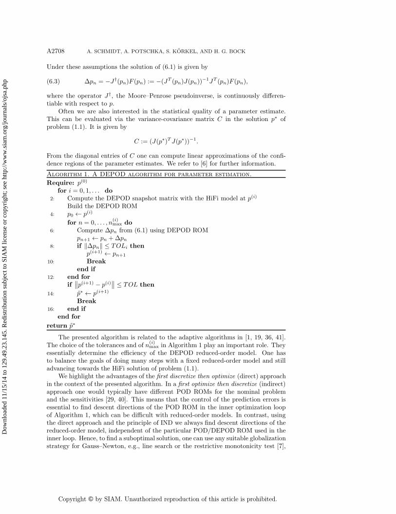
Algorithm 1. A DEPOD algorithm for parameter estimation.

Require: p(0)

for i = 0, 1, . . . do2: Compute the DEPOD snapshot matrix with the HiFi model at p(i)

Build the DEPOD ROM4: p0 ← p(i)

for n = 0, . . . , n(i)max do

6: Compute Δpn from (6.1) using DEPOD ROMpn+1 ← pn +Δpn

8: if ‖Δpn‖ ≤ TOLi thenp(i+1) ← pn+1

10: Breakend if

12: end forif∥∥p(i+1) − p(i)∥∥ ≤ TOL then

14: p∗ ← p(i+1)

Break16: end if

end for

return p∗

The presented algorithm is related to the adaptive algorithms in [1, 19, 36, 41].The choice of the tolerances and of n

(i)max in Algorithm 1 play an important role. They

essentially determine the efficiency of the DEPOD reduced-order model. One hasto balance the goals of doing many steps with a fixed reduced-order model and stilladvancing towards the HiFi solution of problem (1.1).

We highlight the advantages of the first discretize then optimize (direct) approachin the context of the presented algorithm. In a first optimize then discretize (indirect)approach one would typically have different POD ROMs for the nominal problemand the sensitivities [29, 40]. This means that the control of the prediction errors isessential to find descent directions of the POD ROM in the inner optimization loopof Algorithm 1, which can be difficult with reduced-order models. In contrast, usingthe direct approach and the principle of IND we always find descent directions of thereduced-order model, independent of the particular POD/DEPOD ROM used in theinner loop. Hence, to find a suboptimal solution, one can use any suitable globalizationstrategy for Gauss–Newton, e.g., line search or the restrictive monotonicity test [7],

Dow

nloa

ded

11/1

5/14

to 1

29.4

9.23

.145

. Red

istr

ibut

ion

subj

ect t

o SI

AM

lice

nse

or c

opyr

ight

; see

http

://w

ww

.sia

m.o

rg/jo

urna

ls/o

jsa.

php



without updating the reduced model. Moreover, we can exploit the fact that with aDEPOD basis we have an improved POD prediction in the neighborhood of a referenceconfiguration p and, e.g., apply a trust-region method in the inner loop similarly to[2] if necessary.

7. Convergence analysis. In this section we have a closer look at the localconvergence properties of the Gauss–Newton method for parameter estimation prob-lems. By HiFi Gauss–Newton we mean that for the computation of the incrementsΔpn the high-fidelity model is used. Equivalently DEPOD Gauss–Newton means wecompute a Δpn with the reduced-order model.

First, we give a variant of the local contraction theorem [6, 34]. Let F, J , and J†

be defined as in section 6 and P ⊆ Rnp . We denote by N the set of Newton pairs

defined as

N := {(p, p′) ∈ P × P| p′ = p− J†(p)F (p)}.(7.1)

We require the following two conditions on J and J† (see also [12]).Definition 7.1 (ω-condition). The Jacobian J and the pseudoinverse J† satisfy

the ω-condition on P if there exists ω <∞ such that for all ξ ∈ [0, 1] and (p, p′) ∈ N∥∥∥J†(p′)(J (p+ ξ(p′ − p))− J(p)

)(p′ − p)

∥∥∥ ≤ ωξ ‖p′ − p‖2 .Definition 7.2 (κ-condition). J† satisfies the κ-condition on P if there exists

κ < 1 such that for all (p, p′) ∈ N∥∥(J†(p′)− J†(p))(F (p) − J(p)J†(p)F (p))∥∥ ≤ κ ‖p′ − p‖ .

Definition 7.3 (contraction ball). Let δn := κ+ ω2 ‖Δpn‖. If δ0 < 1, we define

the contraction ball

P0 :=

{p ∈ R

np | ‖p− p0‖ ≤ ‖Δp0‖1− δ0

}.

Theorem 7.4 (local contraction theorem). Let J and J† satisfy the ω- and κ-conditions on P. Further, assume that there is an initial guess p0 ∈ P such that wehave

δ0 < 1 and P0 ⊂ P .

Then the following hold.(1) The iterates pn+1 = pn +Δpn are well defined and pn ∈ P0 for all n.(2) There exists p∗ ∈ P0 such that limn→∞ pn = p∗.(3) The a priori estimate ‖pn+l − p∗‖ ≤ ‖Δpn‖

1−δn δln holds.

(4) The steps satisfy ‖Δpn+1‖ ≤ δn ‖Δpn‖.(5) J†(p∗)F (p∗) = 0.The proof is based on the Banach fixed-point theorem and can be found in [6, 34].

The following lemma gives an estimate for the quality of a solution p∗ of DEPODGauss–Newton. For p ∈ P let Δp(p) := −J†(p)F (p) and Δp(p) := −J†(p)F (p) bethe increments computed with the HiFi model and the DEPOD ROM, respectively.Let P0 be the contraction ball of DEPOD Gauss–Newton as in the local contractiontheorem.

Dow

nloa

ded

11/1

5/14

to 1

29.4

9.23

.145

. Red

istr

ibut

ion

subj

ect t

o SI

AM

lice

nse

or c

opyr

ight

; see

http

://w

ww

.sia

m.o

rg/jo

urna

ls/o

jsa.

php



Lemma 7.5. For a given p at which the DEPOD basis is built, assume that theconditions of Theorem 7.4 are satisfied for DEPOD Gauss–Newton on P for p0 = p.Let p∗ be the limit point p∗ from 7.4 (2). Moreover, assume J†, J† ∈ C1(P0). Thenthere is a constant C(p) <∞ independent of p∗ such that we have

‖Δp(p∗)‖ ≤ ε1(k) + (ε2(k) + C(p)) ‖p∗ − p‖+O(‖p∗ − p‖2),(7.2)

where ε1(k) and ε2(k) are constants depending on the DEPOD reconstruction errorsat p.

Proof. As J†, J† ∈ C1(P0) and P0 is compact we have ‖ ddpJ

†(p)‖ <∞ and‖ ddp J

†(p)‖ <∞. Further Δp(p∗) = 0 holds in the solution of DEPOD Gauss–Newton

due to Theorem 7.4. A Taylor expansion of the Gauss–Newton increments at p (defin-ing h := p∗ − p and omitting the argument p of F, J†, F , and J†) yields

‖Δp(p∗)‖ = ‖Δp(p∗)−Δp(p∗)‖

≤∥∥∥∥∥−(J†F +

dJ†Fdp

h

)+

(J†F +

dJ†Fdp

h

)∥∥∥∥∥+O(‖h‖2)=

∥∥∥∥(J†F − J†F)+

(dJ†

dpF − dJ†

dpF

)h+

(J†J − J†J

)h

∥∥∥∥+O(‖h‖2)

=

∥∥∥∥(J†F−J†F)+

(dJ†

dp(F−F+F )− dJ†

dpF

)h+

(J†J−J†J

)h

∥∥∥∥+O(‖h‖2)

≤∥∥∥(J†F − J†F

)∥∥∥︸︷︷︸=ε1(k)

+

∥∥∥∥(dJ†

dpF − dJ†

dpF

)∥∥∥∥︸︷︷︸=C(p)

‖h‖

+

∥∥∥∥dJ†

dp(F − F ) + J†J − J†J

∥∥∥∥︸︷︷︸=ε2(k)

‖h‖+O(‖h‖2)

= ε1(k) + (ε2(k) + C(p)) ‖h‖+O(‖h‖2).

We know from Remark 3.1 and section 5 that we can estimate the reconstructionerrors of the nominal solutions. For the derivatives we assume good approximationsdue to the construction of the POD basis with an extended snapshot matrix. Thus,if we assume the errors ε1 and ε2 to be negligible, then estimate (7.2) is dominated bythe constant C which is an upper bound for the difference between the derivatives ofthe pseudoinverses, computed with the HiFi model and the DEPOD ROM. We canassume in practice that C � ∞ for two reasons. First, due to the κ-conditions, thesecond-order derivatives d

dpJ†(p) and d

dp J†(p) should not be too large. Second, the

residual F should be small if the data can be fitted well through the model.We now formulate the central theorem which yields an estimate on how far a

DEPOD solution deviates from the HiFi solution.Theorem 7.6. For a given p where the DEPOD basis is built, assume that the

conditions of the local contraction theorem hold on P for HiFi and DEPOD Gauss–Newton with p0 ∈ P0 and p0 = p. Let p∗ and p∗ be the corresponding limit points

Dow

nloa

ded

11/1

5/14

to 1

29.4

9.23

.145

. Red

istr

ibut

ion

subj

ect t

o SI

AM

lice

nse

or c

opyr

ight

; see

http

://w

ww

.sia

m.o

rg/jo

urna

ls/o

jsa.

php



from Theorem 7.4 (2). Moreover, require J†, J† ∈ C1(P0). Then we have

‖p∗ − p∗‖ ≤ 1

1− δ(p∗) (ε1(k) + (ε2(k) + C(p)) ‖p∗ − p‖) +O(‖p∗ − p‖2),

where δ(p∗) := κ+ ω2Δp(p

∗) < 1 and ω and κ as in (7.1) and (7.2) for the HiFi, andε1(k), ε2(k), and C(p) as in Lemma 7.5.

Proof. The theorem follows directly from Lemma 7.5 and the a priori estimate (3)in the local contraction theorem, where we set n = l = 0 and choose p0 = p∗ for HiFiGauss–Newton.

From a practical point of view, Theorem 7.6 states that if the DEPODAlgorithm 1terminates, then ‖p∗ − p‖ < TOL and we have found a solution of the HiFi parameterestimation problem up to some given termination tolerance and reconstruction errors.The question arises if there is convergence at all for Algorithm 1. It is clear that forevery first Gauss–Newton step after a DEPOD basis is built (p0 = p0 = p), we have

‖Δp(p)−Δp(p)‖ = ε1(k),

where ε1(k) depends on the DEPOD reconstruction errors. After the first iteration thedifference between the Gauss–Newton directions depends on how much the dynamicsof the underlying PDE system change. The investigation of the convergence of theDEPOD algorithm, given HiFi convergence, is beyond the scope of this paper.

8. Numerical results. In the first two numerical examples we show how withDEPOD we overcome the deficits of the naive POD approach for a simulation togetherwith derivative computation. Then we consider a parameter estimation problem andinvestigate suboptimal solutions of the Gauss–Newton algorithm that are obtainedwith different reduced-order models. In a last numerical example we show the perfor-mance of the DEPOD algorithm.

For all numerical examples we use a parabolic PDE of the form as in (1.2) withdiffusion coefficient D = 0.1 and a nonlinear term of the form

R(y, p) = c1 · p · sin(c2 · y).We consider the domain Ω = [0, 1] together with homogeneous Neumann boundaryconditions. The initial condition is y(0, z) = 1− z. The Galerkin discretization of thespatial dimension for the HiFi model is done with continuous linear finite elementsand N = 201. All considered models are integrated with the implicit Euler scheme

αn+1 = αn + τf(αn+1, p), n = 0, . . . , nsteps − 1,

where nsteps is the number of integration steps and τ is the step size. The nonlinearproblem in each time step is solved by a Newton method. We use αn as the startingvalue for the computation of αn+1 and the number of Newton iterations is fixed at 2.The step size is chosen sufficiently small such that the schemes are stable for the testexample and that in the POD reconstruction error REPOD(t) the time-stepping erroris negligible (see Remark 3.1). We take snapshots at every second integration step asin the considered example we already obtain reconstruction errors close to machineprecision. For the simulation and derivative computation we use the values

p = −3.4 · 10−2, c1 = 2, c2 = 10, τ = 5 · 10−4, nsteps = 1000;

thus, initial and final time are t0 = 0 and tend = 0.5.

Dow

nloa

ded

11/1

5/14

to 1

29.4

9.23

.145

. Red

istr

ibut

ion

subj

ect t

o SI

AM

lice

nse

or c

opyr

ight

; see

http

://w

ww

.sia

m.o

rg/jo

urna

ls/o

jsa.

php



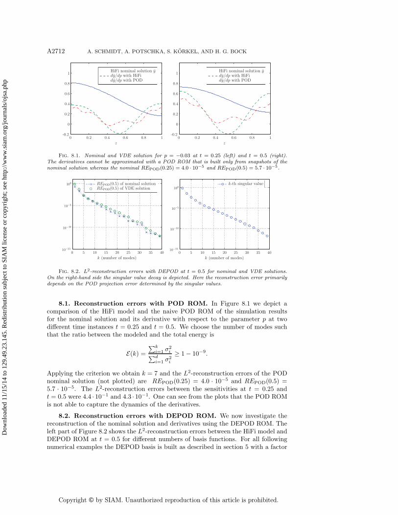
Fig. 8.1. Nominal and VDE solution for p = −0.03 at t = 0.25 (left) and t = 0.5 (right).The derivatives cannot be approximated with a POD ROM that is built only from snapshots of thenominal solution whereas the nominal REPOD(0.25) = 4.0 · 10−5 and REPOD(0.5) = 5.7 · 10−5.

Fig. 8.2. L2-reconstruction errors with DEPOD at t = 0.5 for nominal and VDE solutions.On the right-hand side the singular value decay is depicted. Here the reconstruction error primarilydepends on the POD projection error determined by the singular values.

8.1. Reconstruction errors with POD ROM. In Figure 8.1 we depict acomparison of the HiFi model and the naive POD ROM of the simulation resultsfor the nominal solution and its derivative with respect to the parameter p at twodifferent time instances t = 0.25 and t = 0.5. We choose the number of modes suchthat the ratio between the modeled and the total energy is

E(k) =∑ki=1 σ

2i∑d

i=1 σ2i

≥ 1− 10−9.

Applying the criterion we obtain k = 7 and the L2-reconstruction errors of the PODnominal solution (not plotted) are REPOD(0.25) = 4.0 · 10−5 and REPOD(0.5) =5.7 · 10−5. The L2-reconstruction errors between the sensitivities at t = 0.25 andt = 0.5 were 4.4 · 10−1 and 4.3 · 10−1. One can see from the plots that the POD ROMis not able to capture the dynamics of the derivatives.

8.2. Reconstruction errors with DEPOD ROM. We now investigate thereconstruction of the nominal solution and derivatives using the DEPOD ROM. Theleft part of Figure 8.2 shows the L2-reconstruction errors between the HiFi model andDEPOD ROM at t = 0.5 for different numbers of basis functions. For all followingnumerical examples the DEPOD basis is built as described in section 5 with a factor

Dow

nloa

ded

11/1

5/14

to 1

29.4

9.23

.145

. Red

istr

ibut

ion

subj

ect t

o SI

AM

lice

nse

or c

opyr

ight

; see

http

://w

ww

.sia

m.o

rg/jo

urna

ls/o

jsa.

php



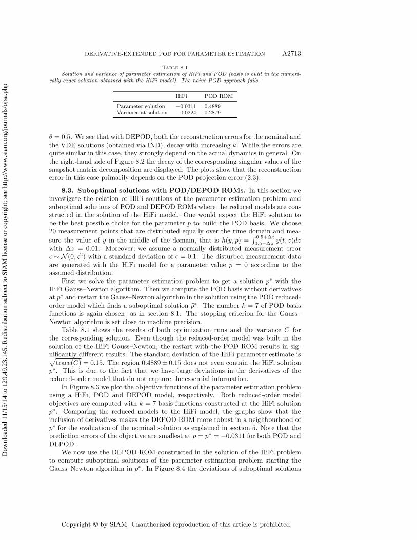
Table 8.1

Solution and variance of parameter estimation of HiFi and POD (basis is built in the numeri-cally exact solution obtained with the HiFi model). The naive POD approach fails.

HiFi POD ROM

Parameter solution −0.0311 0.4889Variance at solution 0.0224 0.2879

θ = 0.5. We see that with DEPOD, both the reconstruction errors for the nominal andthe VDE solutions (obtained via IND), decay with increasing k. While the errors arequite similar in this case, they strongly depend on the actual dynamics in general. Onthe right-hand side of Figure 8.2 the decay of the corresponding singular values of thesnapshot matrix decomposition are displayed. The plots show that the reconstructionerror in this case primarily depends on the POD projection error (2.3).

8.3. Suboptimal solutions with POD/DEPOD ROMs. In this section weinvestigate the relation of HiFi solutions of the parameter estimation problem andsuboptimal solutions of POD and DEPOD ROMs where the reduced models are con-structed in the solution of the HiFi model. One would expect the HiFi solution tobe the best possible choice for the parameter p to build the POD basis. We choose20 measurement points that are distributed equally over the time domain and mea-

sure the value of y in the middle of the domain, that is h(y, p) =∫ 0.5+Δz

0.5−Δzy(t, z)dz

with Δz = 0.01. Moreover, we assume a normally distributed measurement errorε ∼ N (0, ς2) with a standard deviation of ς = 0.1. The disturbed measurement dataare generated with the HiFi model for a parameter value p = 0 according to theassumed distribution.

First we solve the parameter estimation problem to get a solution p∗ with theHiFi Gauss–Newton algorithm. Then we compute the POD basis without derivativesat p∗ and restart the Gauss–Newton algorithm in the solution using the POD reduced-order model which finds a suboptimal solution p∗. The number k = 7 of POD basisfunctions is again chosen as in section 8.1. The stopping criterion for the Gauss–Newton algorithm is set close to machine precision.

Table 8.1 shows the results of both optimization runs and the variance C forthe corresponding solution. Even though the reduced-order model was built in thesolution of the HiFi Gauss–Newton, the restart with the POD ROM results in sig-nificantly different results. The standard deviation of the HiFi parameter estimate is√trace(C) = 0.15. The region 0.4889± 0.15 does not even contain the HiFi solution

p∗. This is due to the fact that we have large deviations in the derivatives of thereduced-order model that do not capture the essential information.

In Figure 8.3 we plot the objective functions of the parameter estimation problemusing a HiFi, POD and DEPOD model, respectively. Both reduced-order modelobjectives are computed with k = 7 basis functions constructed at the HiFi solutionp∗. Comparing the reduced models to the HiFi model, the graphs show that theinclusion of derivatives makes the DEPOD ROM more robust in a neighbourhood ofp∗ for the evaluation of the nominal solution as explained in section 5. Note that theprediction errors of the objective are smallest at p = p∗ = −0.0311 for both POD andDEPOD.

We now use the DEPOD ROM constructed in the solution of the HiFi problemto compute suboptimal solutions of the parameter estimation problem starting theGauss–Newton algorithm in p∗. In Figure 8.4 the deviations of suboptimal solutions

Dow

nloa

ded

11/1

5/14

to 1

29.4

9.23

.145

. Red

istr

ibut

ion

subj

ect t

o SI

AM

lice

nse

or c

opyr

ight

; see

http

://w

ww

.sia

m.o

rg/jo

urna

ls/o

jsa.

php



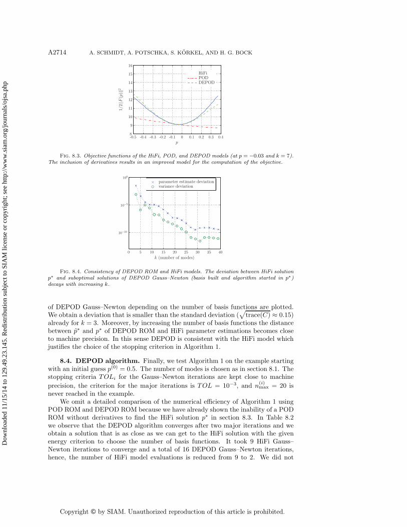
Fig. 8.3. Objective functions of the HiFi, POD, and DEPOD models (at p = −0.03 and k = 7).The inclusion of derivatives results in an improved model for the computation of the objective.

Fig. 8.4. Consistency of DEPOD ROM and HiFi models. The deviation between HiFi solutionp∗ and suboptimal solutions of DEPOD Gauss–Newton (basis built and algorithm started in p∗)decays with increasing k.

of DEPOD Gauss–Newton depending on the number of basis functions are plotted.We obtain a deviation that is smaller than the standard deviation (

√trace(C) ≈ 0.15)

already for k = 3. Moreover, by increasing the number of basis functions the distancebetween p∗ and p∗ of DEPOD ROM and HiFi parameter estimations becomes closeto machine precision. In this sense DEPOD is consistent with the HiFi model whichjustifies the choice of the stopping criterion in Algorithm 1.

8.4. DEPOD algorithm. Finally, we test Algorithm 1 on the example startingwith an initial guess p(0) = 0.5. The number of modes is chosen as in section 8.1. Thestopping criteria TOLi for the Gauss–Newton iterations are kept close to machine

precision, the criterion for the major iterations is TOL = 10−3, and n(i)max = 20 is

never reached in the example.We omit a detailed comparison of the numerical efficiency of Algorithm 1 using

POD ROM and DEPOD ROM because we have already shown the inability of a PODROM without derivatives to find the HiFi solution p∗ in section 8.3. In Table 8.2we observe that the DEPOD algorithm converges after two major iterations and weobtain a solution that is as close as we can get to the HiFi solution with the givenenergy criterion to choose the number of basis functions. It took 9 HiFi Gauss–Newton iterations to converge and a total of 16 DEPOD Gauss–Newton iterations,hence, the number of HiFi model evaluations is reduced from 9 to 2. We did not

Dow

nloa

ded

11/1

5/14

to 1

29.4

9.23

.145

. Red

istr

ibut

ion

subj

ect t

o SI

AM

lice

nse

or c

opyr

ight

; see

http

://w

ww

.sia

m.o

rg/jo

urna

ls/o

jsa.

php



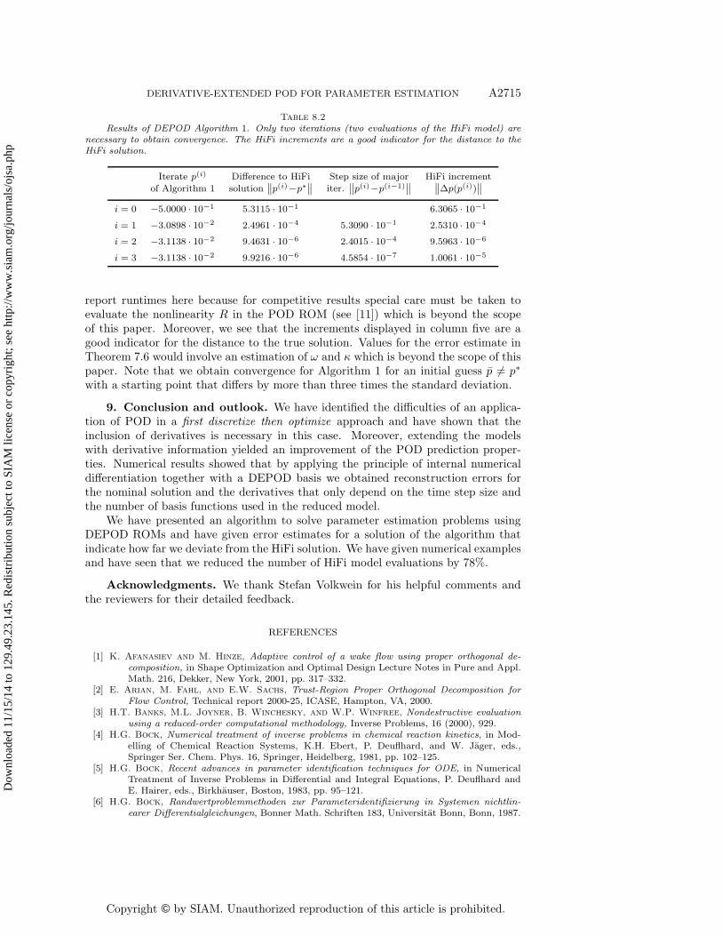
Table 8.2

Results of DEPOD Algorithm 1. Only two iterations (two evaluations of the HiFi model) arenecessary to obtain convergence. The HiFi increments are a good indicator for the distance to theHiFi solution.

Iterate p(i) Difference to HiFi Step size of major HiFi increment

of Algorithm 1 solution∥∥p(i)−p∗

∥∥ iter.

∥∥p(i)−p(i−1)

∥∥

∥∥Δp(p(i))

∥∥

i = 0 −5.0000 · 10−1 5.3115 · 10−1 6.3065 · 10−1

i = 1 −3.0898 · 10−2 2.4961 · 10−4 5.3090 · 10−1 2.5310 · 10−4

i = 2 −3.1138 · 10−2 9.4631 · 10−6 2.4015 · 10−4 9.5963 · 10−6

i = 3 −3.1138 · 10−2 9.9216 · 10−6 4.5854 · 10−7 1.0061 · 10−5

report runtimes here because for competitive results special care must be taken toevaluate the nonlinearity R in the POD ROM (see [11]) which is beyond the scopeof this paper. Moreover, we see that the increments displayed in column five are agood indicator for the distance to the true solution. Values for the error estimate inTheorem 7.6 would involve an estimation of ω and κ which is beyond the scope of thispaper. Note that we obtain convergence for Algorithm 1 for an initial guess p �= p∗

with a starting point that differs by more than three times the standard deviation.

9. Conclusion and outlook. We have identified the difficulties of an applica-tion of POD in a first discretize then optimize approach and have shown that theinclusion of derivatives is necessary in this case. Moreover, extending the modelswith derivative information yielded an improvement of the POD prediction proper-ties. Numerical results showed that by applying the principle of internal numericaldifferentiation together with a DEPOD basis we obtained reconstruction errors forthe nominal solution and the derivatives that only depend on the time step size andthe number of basis functions used in the reduced model.

We have presented an algorithm to solve parameter estimation problems usingDEPOD ROMs and have given error estimates for a solution of the algorithm thatindicate how far we deviate from the HiFi solution. We have given numerical examplesand have seen that we reduced the number of HiFi model evaluations by 78%.

Acknowledgments. We thank Stefan Volkwein for his helpful comments andthe reviewers for their detailed feedback.

REFERENCES

[1] K. Afanasiev and M. Hinze, Adaptive control of a wake flow using proper orthogonal de-composition, in Shape Optimization and Optimal Design Lecture Notes in Pure and Appl.Math. 216, Dekker, New York, 2001, pp. 317–332.

[2] E. Arian, M. Fahl, and E.W. Sachs, Trust-Region Proper Orthogonal Decomposition forFlow Control, Technical report 2000-25, ICASE, Hampton, VA, 2000.

[3] H.T. Banks, M.L. Joyner, B. Winchesky, and W.P. Winfree, Nondestructive evaluationusing a reduced-order computational methodology, Inverse Problems, 16 (2000), 929.

[4] H.G. Bock, Numerical treatment of inverse problems in chemical reaction kinetics, in Mod-elling of Chemical Reaction Systems, K.H. Ebert, P. Deuflhard, and W. Jager, eds.,Springer Ser. Chem. Phys. 16, Springer, Heidelberg, 1981, pp. 102–125.

[5] H.G. Bock, Recent advances in parameter identification techniques for ODE, in NumericalTreatment of Inverse Problems in Differential and Integral Equations, P. Deuflhard andE. Hairer, eds., Birkhauser, Boston, 1983, pp. 95–121.

[6] H.G. Bock, Randwertproblemmethoden zur Parameteridentifizierung in Systemen nichtlin-earer Differentialgleichungen, Bonner Math. Schriften 183, Universitat Bonn, Bonn, 1987.

Dow

nloa

ded

11/1

5/14

to 1

29.4

9.23

.145

. Red

istr

ibut

ion

subj

ect t

o SI

AM

lice

nse

or c

opyr

ight

; see

http

://w

ww

.sia

m.o

rg/jo

urna

ls/o

jsa.

php



[7] H.G. Bock, E.A. Kostina, and J.P. Schloder, On the role of natural level functions toachieve global convergence for damped Newton methods, in System Modelling and Opti-mization. Methods, Theory and Applications, M.J.D. Powell and S. Scholtes, eds., Kluwer,Boston, 2000, pp. 51–74.

[8] T. Bui-Thanh, K. Willcox, O. Ghattas, and B. van Bloemen Waanders, Goal-oriented,model-constrained optimization for reduction of large-scale systems, J. Comput. Phys., 224(2007), pp. 880–896.

[9] K. Carlberg and C. Farhat, A low-cost, goal-oriented “compact proper orthogonal decom-position” basis for model reduction of static systems, Internat. J. Numer. Methods Engrg.,86 (2011), pp. 381–402.

[10] D. Chapelle, A. Gariah, and J. Sainte-Marie, Galerkin approximation with proper orthog-onal decomposition: New error estimates and illustrative examples, ESAIM: Math. Model.Numer. Anal., 46 (2012), pp. 731–757.

[11] S. Chaturantabut and D.C. Sorensen, Nonlinear model reduction via discrete empiricalinterpolation, SIAM J. Sci. Comput., 32 (2010), pp. 2737–2764.

[12] P. Deuflhard, Newton Methods for Nonlinear Problems: Affine Invariance and AdaptiveAlgorithms, Springer, Berlin, 2004.

[13] F. Diwoky and S. Volkwein, Nonlinear boundary control for the heat equation utilizing properorthogonal decomposition, in Fast Solution of Discretized Optimization Problems, K.-H.Hoffmann, R. H. W. Hoppe, and V. Schulz, eds., Internat. Ser. Numer. Math. 138, Birk-hauser, Basel, 2001, pp. 267–278.

[14] M. Fahl, Trust-Region Methods for Flow Control Based on Reduced Order Modelling, Ph.D.thesis, University of Trier, Trier, Germany, 2000.

[15] A. Griewank, Evaluating Derivatives, Principles and Techniques of Algorithmic Differentia-tion, Front. Appl. Math. 19, SIAM, Philadelphia, 2000.

[16] A. Hay, I. Akhtar, and J.T. Borggaard, On the use of sensitivity analysis in model reduc-tion to predict flows for varying inflow conditions, Internat. J. Numer. Methods Fluids, 68(2012), pp. 122–134.

[17] A. Hay, J.T. Borggaard, and D. Pelletier, Local improvements to reduced-order modelsusing sensitivity analysis of the proper orthogonal decomposition, J. Fluid Mech., 629(2009), pp. 41–72.

[18] M. Hinze, R. Pinnau, M. Ulbrich, and S. Ulbrich, Optimization with PDE-Constraints,Springer, New York, 2009.

[19] M. Hinze and S. Volkwein, Proper orthogonal decomposition surrogate models for nonlineardynamical systems: Error estimates and suboptimal control, in Dimension Reduction ofLarge-Scale Systems, Lect. Notes Comput. Sci. Eng. 45, Springer, Berlin, 2005, pp. 261–306.

[20] M. Hinze and S. Volkwein, Error estimates for abstract linear-quadratic optimal control prob-lems using proper orthogonal decomposition, Comput. Optim. Appl., 39 (2008), pp. 319–345.

[21] C. Homescu, L.R. Petzold, and R. Serban, Error estimation for reduced-order models ofdynamical systems, SIAM J. Numer. Anal., 43 (2005), pp. 1693–1714.

[22] M. Kahlbacher and S. Volkwein, Estimation of regularization parameters in elliptic opti-mal control problems by POD model reduction, in System Modelling and Optimization,W. Mitkowski A. Korytowski, K. Malanowski, and M. Szymkat, eds., Springer-Verlag,Berlin, 2009, pp. 307–318.

[23] M. Kahlbacher and S. Volkwein, POD a-posteriori error based inexact sqp method forbilinear elliptic optimal control problems, ESAIM: Math. Model. Numer. Anal., 46 (2012),pp. 491–511.

[24] E. Kammann, F. Troltzsch, and S. Volkwein, A method of a-posteriori error estimationwith application to proper orthogonal decomposition, Konstanzer Schriften in Mathematik299, http://kops.ub-konstanz.de/handle/urn:nbn:de:bsz:352–184660 (2012).

[25] S. Korkel, Numerische Methoden fur Optimale Versuchsplanungsprobleme bei nichtlinearenDAE-Modellen, Ph.D. thesis, Universitat Heidelberg, Heidelberg, 2002.

[26] K. Kunisch and S. Volkwein, Control of the Burgers equation by a reduced-order approachusing proper orthogonal decomposition, J. Optim. Theory Appl., 102 (1999), pp. 345–371.

[27] K. Kunisch and S. Volkwein, Galerkin proper orthogonal decomposition methods for parabolicproblems, Numer. Math., 90 (2001), pp. 117–148.

[28] K. Kunisch and S. Volkwein, Galerkin proper orthogonal decomposition methods for a generalequation in fluid dynamics, SIAM J. Numer. Anal., 40 (2002), pp. 492–515.

[29] K. Kunisch and S. Volkwein, Proper orthogonal decomposition for optimality systems,ESAIM: Math. Model. Numer. Anal., 42 (2008), pp. 1–23.

Dow

nloa

ded

11/1

5/14

to 1

29.4

9.23

.145

. Red

istr

ibut

ion

subj

ect t

o SI

AM

lice

nse

or c

opyr

ight

; see

http

://w

ww

.sia

m.o

rg/jo

urna

ls/o

jsa.

php



[30] K. Kunisch and S. Volkwein, Optimal snapshot location for computing POD basis functions,ESAIM: Math. Model. Numer. Anal., 44 (2010), pp. 509–529.

[31] A. Noor and J. Peters, Reduced basis technique for nonlinear analysis of structures, AIAAJ., 18 (1980), pp. 455–462.

[32] Z. Ostrowski, R.A. Bialecki, and A.J. Kassab, Advances in application of proper orthogonaldecomposition in inverse problems, in Proceedings of the 5th International Conference onInverse Problems in Engineering: Theory and Practice, Cambridge, UK, 2005.

[33] T. Porsching, Estimation of the error in the reduced basis method solution of nonlinear equa-tions, Math. Comp., 45 (1985), pp. 487–496.

[34] A. Potschka, A Direct Method for the Numerical Solution of Optimization Problems withTime-Periodic PDE Constraints, Ph.D. thesis, University of Heidelberg, Heidelberg, 2012.

[35] M. Rathinam and L.R. Petzold, A new look at proper orthogonal decomposition, SIAM J.Numer. Anal., 41 (2003), pp. 1893–1925.

[36] S.S. Ravindran, Adaptive reduced-order controllers for a thermal flow system using properorthogonal decomposition, SIAM J. Sci. Comput., 23 (2002), pp. 1924–1942.

[37] E.W. Sachs and S. Volkwein, POD Galerkin approximations in PDE-constrained optimiza-tion, GAMM Mitt. Ge., Math. Mech. Angew., 33 (2010), pp. 194–208.

[38] J. Stoer and R. Bulirsch, Introduction to Numerical Analysis, Springer, New York, 2002.[39] F. Troltzsch, Optimal control of partial differential equations, Grad. Stud. Math. 112, AMS,

Providence, RI, 2010.[40] F. Troltzsch and S. Volkwein, POD a-posteriori error estimates for linear-quadratic opti-

mal control problems, Comput. Optim. Appl., 44 (2009), pp. 83–115.[41] C. Winton, J. Pettway, C.T. Kelley, S. Howington, and O.J. Eslinger, Application

of proper orthogonal decomposition (POD) to inverse problems in saturated groundwaterflow, Adv. Water Res., 34 (2011), pp. 1519–1526.

Dow

nloa

ded

11/1

5/14

to 1

29.4

9.23

.145

. Red

istr

ibut

ion

subj

ect t

o SI

AM

lice

nse

or c

opyr

ight

; see

http

://w

ww

.sia

m.o

rg/jo

urna

ls/o

jsa.

php

derivative-extended pod reduced-order modeling for parameter estimation

Documents