department of: technical programs principles of digital ... · principles of digital microwave this...
TRANSCRIPT

Department of: Technical programs
Principles of digital
microwave


1 Introduction to Digital microwave Radio pages (1-59)
Sub – Sections
2 VHF/UHF/Microwave Radio Propagation pages (1-34)
3 Microwave Antenna System pages (1-64)
Principles of digital
Microwave
This document consists of 157 pages


Chapter 1: Introduction to Digital microwave Radio Technology
1 TS53TX11St
Chapter 1 : Introduction to Digital microwave
Radio Technology
Aim of study
Recognize the transmission media types, Point-to-point digital
microwave radio, Microwave Radio Configurations, frequency
planning.
Contents pages
1.1 Telecommunication 3
1.2 Microwave Communication 5
1.3 Atmosphere Layer 5
1.4 Microwave Definition 6
1.5 Components of Microwave Systems 6
1.6 Introduction to DMR 7
1.7 Benefits to Fixed Wire, GSM, CDMA, WLL and PTT 12
1.8 Microwave Radio Configurations 14
1.9 Equipment Considerations 15
1.10 Network Design Process 17
1.11 Regulatory Considerations 20
1-12 Summary 26
1.13 Microwave Repeaters 27

Chapter 1: Introduction to Digital microwave Radio Technology
2 TS53TX11St
1-14 Antenna types 28
1-15 Microwaves 28
1-16 Antannas 30
1-17 Generators of Microwave Signals And Noise Effect 38

Chapter 1: Introduction to Digital microwave Radio Technology
3 TS53TX11St
Chapter 1
Introduction to Digital microwave Radio Technology
1.1 Telecommunication
1.1.1 Transmission Media
- Guided transmission
- Unguided transmission
Guided transmission
Cable Type Bandwidth
a. Open Wire Open Cable 0-5 MHz
b. Twisted Pair Twisted Pair 0-100 MHz
c. Coaxial Cable Coaxial Cable 0-600 MHz
d. Optical Fiber Optical Fiber 0-1 GHz
Telecommunicati
on
Wireless
Global
Wire
Terrestrial
Analog Digital
FM PM AM QPSK CDMA PSK

Chapter 1: Introduction to Digital microwave Radio Technology
4 TS53TX11St
Unguided transmission
RF – Propagation
1. Ground Wave
Figure (1-1) Ground Wave Propagation
2. Ionosphere
Figure (1-2) Ionosphere Propagation
3. Line of sight (LOS) Propagation
Figure (1-3) Microwave Transmission
Earth Home
Radio
Tower
Atmosphere
Radio
Tower
Home
Earth
Ionosphere
Transmitter
Receiver
Repeater

Chapter 1: Introduction to Digital microwave Radio Technology
5 TS53TX11St
1.2 Microwave Communication
Figure (1-4)
1.3 Atmosphere Layer
Figure (1-5)
IONOSPHERE RADIO
TV
Site A Site B

Chapter 1: Introduction to Digital microwave Radio Technology
6 TS53TX11St
1.4 Microwave Definition
Advantages
a. They require no right of way acquisition between towers.
b. They can carry high quantities of information due to their high
operating frequencies.
c. Low cost land purchase: each tower occupies small area.
d. High frequency/short wavelength signals require small antenna.
Disadvantages
a. Attenuation by solid objects: birds, rain, snow and fog.
b. Reflected from flat surfaces like water and metal.
c. (split) around solid objects
d. Refracted by atmosphere, thus causing beam to be
projected away from receiver.
1.5 Components of Microwave Systems
Microwave Transceivers
1. Antenna
2. Transmitter
3. Receiver
4. Control unit
5. Power supply
6. Amplification
Chapter 1: Introduction to Digital microwave Radio Technology
7 TS53TX11St
1.6 Introduction to DMR
Point-to-point digital microwave radio (DMR), as the name implies, is a
digital transmission technology that provides a wireless radio link operating at
microwave frequencies between two points. A terminal at one end of the link
communicates exclusively with a complementary terminal at the other end of
the link. Each terminal is fitted to a parabolic dish antenna and
communication is by line-of-sight beams between the dishes.
DMP is very flexible and does not depend on other elements such as satellite,
cable, or optical fibre). Compunction distances can be a short as a few meters
(eg across the street between buildings in the city) or very long (up to 80Km)
in the country. To achieve line-of-sight, antennas and at least a portion of the
terminal are typically mounted on rooftops, on hills of on towers. Links can
also be daisy-chained to avoid major obstructions or to cover virtually endless
communication distances.
DMR links can be used to carry a wide variety of traffic. In the
telecommunications industry, they are used to carry data, voice, fax while in
the broadcast industry they carry video and audio signals. In the wireless data
communications market, DMR links carry Ethernet traffic between Local
Area Network (LAN) sites. Other applications include security, telemetry,
monitor and control and many other applications requiring transport of
digitized information.
Radio spectrum usage and data transmission standards are subject to
regulatory frameworks throughout the world, in the interests of efficient
spectrum usage and interoperability. The European Telecommunications
Standards Institute (ETSI) incorporates International Telecommunications
Union (ITU) recommendations into the European regulatory framework, and
these are followed in much of the rest of the world. The Federal

Chapter 1: Introduction to Digital microwave Radio Technology
8 TS53TX11St
Communications Commission (FCC) oversees radio spectrum usage in the
US, where American National Standards Institute (ANSI) data standards are
typically used.
For telecommunications, the traffic usually carried by DMR is structured in a
hierarchy of data rates and formats known collectively as Plesiochronous
Digital Hierarchy (PDH) according to standards set by the ITU and ANSI.
The microwave operating frequencies and the structure of the actual
frequencies and bandwidths used are standardized by the ITU and FCC into
operating bands. The frequency chosen for a particular link will depend upon
many factors including the region (higher frequencies are attenuated by rain
and cannot be used in tropical environments) and the service (there are more
frequency allocations available at higher frequencies and they are used in
areas of higher traffic density, such as cities).
The products offered by Codan have operating frequencies ranging from
7GHz to 38GHz with data interfaces allowing flexible combinations of PDH
data streams and Ethernet traffic. The maximum aggregate data rate that can
be carried is 52Mbs, depending on the data standards and spectrum licensing
arrangements in the country of use.
A substantial driver for the development of the DMR industry in recent times
has been deregulation of the telecommunications industry in many countries.
Today, fixed and mobile network operators and even private users can
establish their own networks throughout the world, with the right to provide
the transmission infrastructure independently of the dominant carriers. DMR
allows private voice and data networks and cellular networks to be established
very quickly, efficiently and at substantially lower cost than cable systems.
As more countries deregulate their telecommunications infrastructure, as
communications services are extended to more regions of the world, and as

Chapter 1: Introduction to Digital microwave Radio Technology
9 TS53TX11St
the demand for ever higher data rate capacities expands, the market for
communications by digital microwave radio is expected to expand rapidly.
Let us now focus on the applications of digital microwave radio and its main
users, while also trying to explain the reasons for an explosive growth in
demand for such products.
1.6.1 Cellular Applications
The greatest growth area for the use of digital microwave radio is currently
associated with the emergence of new cellular mobile operators as part of a
liberalized telecommunications environment. It is normal for newly licensed
operators to be granted the rights to self-provide the transmission
infrastructure.
It is also the trend that the terms of such competitive licenses commit the
operators to challenging operational obligations, i.e. to provide service
throughout a certain percentage of the country within an ambitious time
frame. Furthermore, operators need to provide service at the earliest
opportunity to realize revenues in line with their business plans.
Faced with this scenario, mobile operators are very conscious of the
advantages of digital microwave radio. The speed of installation and
flexibility to upgrade in line with network requirements has meant that almost
all mobile operators who are independent from the PTT organizations and
have the right to self-provide have chosen digital microwave radio as the
interconnect solution for base stations.

Chapter 1: Introduction to Digital microwave Radio Technology
10 TS53TX11St
1.6.2 PTT fixed network applications
Newly licensed competitive operators are not the only users of microwave
radio, and a number of factors are leading to a growing demand from
incumbent fixed network operators. With the growing liberalization in
telecommunications, PTT’s are now finding themselves operating in a more
competitive environment. As a result, users are being offered greater quality
of service and learning that they can demand more from service operators.
Time scale for provision of service is a major differentiator for a PTT
operator wishing to offer competitive services.
Because of the flexibility of microwave radio and the ease and speed of
installation, these products are increasingly finding their way into PTT access
or back-haul networks. Elsewhere, in many developing markets, operators
who wish to provide international telephone and data services to customers
Figure (1-6) GSM Application

Chapter 1: Introduction to Digital microwave Radio Technology
11 TS53TX11St
are utilizing microwave direct from exchanges to the customer premises in
order to bypass local networks that are often inadequate.
Utilizing microwave radio as an access medium direct to a customer's
premises has been common for a number of years. However, a number of
factors are leading to an increase in this application.
New operators are being licensed who, unlike the entrenched PTT’s, do not
have established cable networks but do have a need to connect customers
quickly. Likewise, microwave radio is commonly used within these networks
in back-haul applications, i.e. connecting from a strategic distribution point
within the network (such as a business park) back into the switched network.
Figure (1-7) illustrates a few of these applications.
Figure (1-7) PTT Fixed Network

Chapter 1: Introduction to Digital microwave Radio Technology
12 TS53TX11St
1.6.3 Private network applications
In certain parts of the world, utility and government organizations have long
had discretionary rights to build their own networks, and have historically
been users of microwave radio. With growing liberalization, many other
private users are recognizing the benefits of digital microwave radio. The
applications in this arena are quite varied, ranging from the users who wish to
interconnect a network of PBXs in multiple locations throughout a region, to
the smaller users who simply wish to interconnect two LANs in two different
buildings within a single site.
1.7 Benefits to Fixed Wire, GSM, CDMA, WLL and PTT operators
The above network applications have mentioned many reasons why a network
operator, given the right to self-provide transmission infrastructure, should
choose microwave radio as opposed to utilizing leased lines or implementing
their own cable based systems. In summary, the advantages of microwave
radio systems are as follows.
Economical compared to fibre or leased lines - Significant whole-life
cost savings can be achieved by building self-provided networks as
opposed to leasing services from the local PTT
Ownership - A self-provided transmission network remains under the
control and ownership of the end user, which removes a dependency
upon the incumbent PTT (often a competitor) and provides operational
benefits.
Flexibility - Modern microwave radio architecture has been designed to
provide a high degree of flexibility in terms of distance and traffic
capacity, enabling links to be designed to precisely fit operator

Chapter 1: Introduction to Digital microwave Radio Technology
13 TS53TX11St
requirements and local conditions. Link capacities can also be field
upgraded to cater to a network's growing traffic requirements as
subscriber numbers increase
Reliability - Self-provided networks can be planned to provide a higher
quality of service than often guaranteed by the PTT. Radio based
solutions can be engineered to provide availability at least equivalent to
cable based systems when viewed over many years, during which it is
possible that a cable will be dug up or severed several times.
Right of way not required - Laying cable requires time-consuming and
potentially costly rights of way to cross third-party property. Microwave
radio avoids this problem by utilizing the air that is a free resource.
Speed of Installation - A microwave link can, in the majority of
circumstances, be installed and commissioned in a much shorter period
of time than cable based alternatives, because a microwave link does not
require the same degree of civil works associated with laying cables
Ability for re-deployment - Microwave radio links can be easily
removed and re-deployed to another geographical area, without leaving
valuable assets in the ground
Availability - Microwave radio is commercially available and can be
supplied in extremely short time scales
Gives a competitive edge - Finally, microwave radio gives a new
operator the ability to minimize time to market, hence maximizing
revenue.
Microwave radio provides a clear, cost-effective and feasible solution
against leased lines or self provided cable-based alternatives.
Chapter 1: Introduction to Digital microwave Radio Technology
14 TS53TX11St
1.8 Microwave Radio Configurations
Microwave radio systems can be found in various configuration types,
including:
Indoor rack mounted. In this configuration, the radio terminal consists
of an indoor-mounted baseband shelf and RF transceiver, with a
parabolic antenna connected to the indoor equipment via wave-guide.
This configuration provides the advantages of:
Lightening protection – no electronic equipment on the tower
Ease of maintenance – no need to climb the tower
The main disadvantage is that you need to use expensive waveguide to
connect the RF equipment to the antenna. These configurations are often
deployed in extremely cold areas where ice forming on the tower prevents
maintenance access. Installations in corrosive atmosphere situations like
certain mining sites where outdoor mounted equipment may be damaged
by the highly acidic emissions also use indoor mounted equipment.
Split mount, In this configuration, the radio terminal consists of an
indoor-mounted baseband shelf, an outdoor-mounted RF transceiver,
and a parabolic antenna. The indoor unit provides the interfaces to
other equipment, and is separated from the RF transceiver via
standard coaxial cable by typically up to 300 meters.
This is by far the most common type of configuration for PDH
microwave link installations.
The main advantage of this type of configuration is the ease and cost
of the installation through the use of a single coaxial cable to connect
the indoor and outdoor equipment.

Chapter 1: Introduction to Digital microwave Radio Technology
15 TS53TX11St
The RF transceiver, when mounted outdoors, can be mounted directly
behind the parabolic antenna, or the RF unit can be mounted remotely
from the antenna. Systems are available in either non-protected (1+0)
or protected (1+1) configurations.
A protected terminal provides full duplication of active elements in a
terminal (i.e. both the RF transceiver and the baseband components), in
a "hot standby" mode to protect the user against equipment failure.
Automatic switching to the standby system during periods of
equipment failure allow the operator to deliver the required service to
their customers without any down time.
Space diversity (2 antenna) is a variation on the hot standby
configuration that provide protection against reflections from the
ground and other similar propagation anomalies. The theory behind this
type of configuration is that when the microwave path causes a problem
with one antenna, statistically speaking, the other one is able to operate
without being affected by the problem. The advanced space diversity
switching algorithm used in the Codan 8800 series optomises link
performance under difficult conditions by selecting the best path on a
frame-by-frame basis.
Digital Microwave Radio Codan 8800 series
1.9 Equipment Considerations
When selecting appropriate radio equipment for deployment within a
Telecommunication Network, the following characteristics/ specifications are
among those that should be considered:
Radio performance - A modern radio design will incorporate one or
more facilities to counter the adverse effects of the radio wave

Chapter 1: Introduction to Digital microwave Radio Technology
16 TS53TX11St
propagation through the atmosphere, generally seen as fading, or
reduction, of the received signal. Fading countermeasures include
interference rejection capability, forward error correction (FEC), and
Automatic Transmit Power Control (ATPC) and space diversity
arrangements.
All these features are supported by the Codan 8800 series. Additionally,
the Codan 8800 uses Continuous Phase Modulation (CPM), which is
inherently robust in the presence of propagation impairments.
High spectral efficiency - An efficient modulation scheme to minimize
channel bandwidth is a great benefit when planning the radio network,
and is some times a prerequisite of the regulatory authority.
The Codan 8800 series uses 4-state CPM, which provides the spectral
efficiency required in most countries.
High system gain - This is a function of the radio output power and
received signal threshold.
The Codan 8800 series compares favorably with most competing
products.
Low background BER - This is a measure of the performance (bit error
rate) of the radio equipment in the absence of interference induced by
propagation anomalies, and should ideally be less than 10-12
.
The Codan 8800 is specified as to perform with a Background BER of
10-15
.
High environmental specification - Essential for reliable operation in
harsh environments when equipment is located externally. Equipment
must have a minimum operational temperature range of –30oC to +55
oC

Chapter 1: Introduction to Digital microwave Radio Technology
17 TS53TX11St
for outdoor equipment. Other important factors are ingress protection
against water and dust or sand, and corrosion resistance.
The Codan 8800 is specified from –33oC to +55
oC.
Equipment reliability and maintainability - Important in ensuring a low
life-cycle cost is the ability of the equipment to operate for long periods
without failure (high mean time between failures, or MTBF). Equally,
when failures occur they must be easily and rapidly repaired (low mean
time to repair, or MTTR). This will be facilitated by spares
commonality across a range of capacities and frequency ranges. An
operator must also determine which links require protection, based
upon the criticality of each link and the existence of alternative traffic
routing in the case of failure.
The Codan 8800 series MTBF is expected to be in excess of 30 years.
The mean time to repair a Codan 8800 series link by a trained field
service engineer is less than 1 hour.
1.10 Network Design Process
To reach the stage where a microwave radio link can be deployed and brought
into service, several steps must be successfully completed, often in an
iterative process, leading to a final link design.
These steps are briefly:
Determine design objectives, that is:
Availability target for network
Availability target for radio path
Required capacity (current and future)

Chapter 1: Introduction to Digital microwave Radio Technology
18 TS53TX11St
Maintainability, i.e. protected or non- protected
Determine and produce network design. A network design is required to
establish all of the nodes within the network that require transmission
links between them. This can then be developed to become the main
reference document for network planning and implementation
Determine local frequency availability and regulatory restrictions.
Select and survey sites
Establish existence of line-of-sight
Detailed network design - frequency planning.
1.10.1 Network Topologies
Figure (1-8) , Figure (1-9) depict two common configurations that are adopted
for the transmission system of a GSM Network.
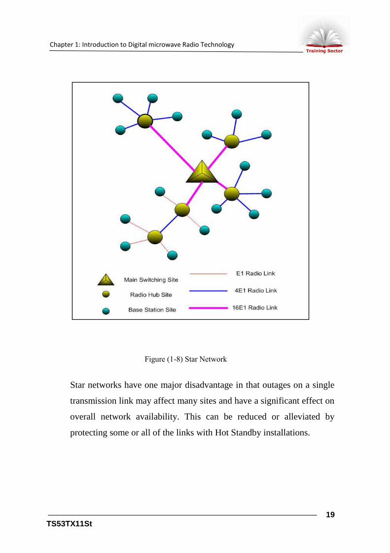
Star network
A star network topology will contain one or more hub sites at strategic
locations that serve spurs or chains of subordinate sites from the
centralized hub. A star network can be multilayered in that some of the
nodes in a spur may be hub sites for further subordinate spurs.
Chapter 1: Introduction to Digital microwave Radio Technology
19 TS53TX11St
Star networks have one major disadvantage in that outages on a single
transmission link may affect many sites and have a significant effect on
overall network availability. This can be reduced or alleviated by
protecting some or all of the links with Hot Standby installations.
Figure (1-8) Star Network

Chapter 1: Introduction to Digital microwave Radio Technology
20 TS53TX11St
Ring network
Ring structures can be successfully achieved in PDH networks if the
necessary routing and grooming intelligence exists at all appropriate
equipment that is connected to the DMR links in the network.
The capacity of all of the links in a ring has to be sufficient to support
all sites in the loop, so that some links have increased capacity over the
equivalent star structure.
1-11 Regulatory Considerations
Frequency spectrum is a valuable resource and is generally subject to
appropriate planning and management to prevent misuse and
interference between the many and varied applications. National
administrations will allocate some or all these bands for fixed
microwave radio use in line with local requirements. Before network
Figure (1-9) Ring Network

Chapter 1: Introduction to Digital microwave Radio Technology
21 TS53TX11St
planning commences, an operator must determine available frequency
bands and channel plans specific to that country. Often, and preferably,
an operator may be able to obtain a number of frequency allocations as
a block for nation wide use thus enabling him to perform his own
network planning in advance without risk of interference from other
users.
Most regulatory authorities also operate a local link length policy, where
the length of a particular path will determine what frequency bands are
available for the operator to choose from. Typically, the shorter the path
the higher the frequency required.
The local requirement for equipment type approval will also vary from
country to country, ranging from a simple paperwork exercise to a full
product test program to local standards. Type approval is generally the
responsibility of the radio supplier, but an operator should ensure that all
requirements are satisfied before links are deployed.
Other limitations imposed by authorities can also have an impact upon
microwave radio deployment - for example, tower height restrictions or
limitations upon antenna size. These factors can restrict effective radio
lengths at the planning stage and should be ascertained in advance of
the detailed link design stage.
1-11-1 Site selection and survey
Selection of a suitable microwave radio site must encompass a number
of issues. There are economical and engineering benefits to be gained
by maximizing the sharing of infrastructure and sites between the
various types of elements in the network, particularly regarding
expensive civil infrastructure such as towers and equipment housings.
It is becoming more common for competing operators to share the

Chapter 1: Introduction to Digital microwave Radio Technology
22 TS53TX11St
expensive and common portion of site construction like towers, shelters
and mains power connection.
The location of good microwave sight, particularly in relation to hub
sites, will be relatively high points to provide the maximum line of site
availability. This information should be fed back into the network plan
as it can affect both routing and path planning.
Attention should be given to future growth requirements in all areas,
especially if the site is likely to develop into a future hub. It is always
wise to inform the landowner of any potential future growth to prevent
problems at a later date.
Attention should be paid to any local authority planning restrictions and
approvals for structures or antenna installations planned. Such
restrictions could be found to eliminate a site at a very late stage of the
process and cause much wasted effort.
An operator should aim to perform only one site survey to minimize
costs. Equipment installation requirements must be confirmed
considering amongst other things, power, accommodation, and
environmental conditions. The ease of service access for maintenance
personnel, particularly tower mounted equipment can have significant
impact on costs and repair time. Required loading needs to be
calculated if new tower installations are proposed, and these must take
into account the antenna wind and ice loading.
New terminals being added to an existing tower require calculations
that ensure incremental loading can be accommodated. Cable and/or
waveguide routing should be checked, including length and securing.
Digital Microwave Radio Codan 8800 series

Chapter 1: Introduction to Digital microwave Radio Technology
23 TS53TX11St
1-11-2 Frequency bands
The International Telecommunication Union (ITU) ITU-R organization
defines a number of specific frequency bands that are allocated to fixed
services - i.e. for microwave point-to-point links. Table 1-1 shows the
ITU-R bands covered the Codan 8800 series, and outlines the usage for
digital telecommunications purposes.
Table (1-1): Common Fixed Microwave Link Frequency Bands
Table (1-1) Common Fixed Microwave Link Frequency Bands
Different frequency bands are subject to differing propagation criteria,
which results in attenuation in the link received signal. As a general

Chapter 1: Introduction to Digital microwave Radio Technology
24 TS53TX11St
rule, the higher the frequency band, the shorter the usable distance of
the link.
In the extreme case, use of frequency bands above 20 GHz in tropical
areas will limit path length to just a few kilometres.
Frequency management organizations will also make most effective
use of frequency spectrum by imposing a link length policy; i.e. shorter
links will be licensed only in the higher frequency bands and vice-
versa.
1-11-3 Confirmation of line of sight
A clear transmission path must exist between the two link nodes of any
microwave radio link.
Furthermore, as the radio wave disperses as it moves away from the
source, there must exist additional clearance over any obstructions to
prevent attenuation of the transmitted signal. This additional clearance,
known as the Fresnel zone, differs for the frequency band of the radio
path, where higher frequency translates into a smaller clearance
requirement.
See Figure below.
Figure (1-10) Line of Sight

Chapter 1: Introduction to Digital microwave Radio Technology
25 TS53TX11St
Line of sight between two sites can be confirmed by either map-based
studies or direct visual survey. In either event, the surveyor must allow
for future obstructions that may impinge the radio path. These can be
due to various causes, such as new buildings, tree growth, cranes, etc.
1-11-4 Frequency planning
Frequency planning is the coordination of link frequencies to minimize
any interference between links within the network and those operated
by other users. In some instances, the local regulatory authority
undertakes frequency planning. However, if a block allocation has been
obtained, then planning will be the responsibility of the operator.
Several factors must be considered that will affect the calculations of
interference that will determine the optimum channel frequency for
each radio link.
There are a number of equipment performance parameters that become
relevant when considering interference within a microwave network.
These include:
Path availability target considerations, since higher availabilities
will require higher levels of protection from interference and
hence increase planning difficulties. The level of availability must
be considered in conjunction with the network plan and the
physical position of the link. Availability targets can be relaxed for
the lower capacity outer links where short outages may not cause
disruption to subscriber services, due to overlapping coverage
from adjacent cells, or the availability of diverse routing
Radiated transmit power (EIRP)

Chapter 1: Introduction to Digital microwave Radio Technology
26 TS53TX11St
Link operating frequencies
The channel plan
The Carrier to Interference (C/l) performance of the equipment
which determines how well the radio equipment can discriminate
the wanted signal in the presence of interference
Antenna characteristics, such as radiation pattern envelope (RPE),
gain and front-to- back ratio.
1-12 Summary
There are numerous economic and operational benefits in utilizing
digital microwave radio in a transmission network. Radio presents an
attractive alternative to both PTT-provided leased lines or self-provided
cable based systems, and major operational advantages accrue from the
fact that, being a wireless technology, microwave radio can be
installed, commissioned and re-deployed easily and quickly.
For a new telecommunications operator in an existing or emerging
competitive environment, these advantages can provide the crucial edge
for success, and enable the operator to establish an operational network
in a matter of months, thereby providing early revenue for re-
investment and return to shareholders and other investors.
Many operators are now recognizing these benefits, and we are seeing
significant growth in demand emerging, specifically from newly
licensed cellular operators, as well as competitively licensed fixed
network operators and even the incumbent PTT’s who have to operate
in the new competitive environment.
PDH digital microwave radio's place as a key network element is well
established and has a bright future.

Chapter 1: Introduction to Digital microwave Radio Technology
27 TS53TX11St
Transmitting Path
Figure (1-11) Transmitter Path
Receiving Path
Figure (1-12) Receiver Path
1-13 Microwave Repeaters
B.B
+
I.F.
+
Carrier
B.B.
+
Intermediate
Freq. Base
Band
Multiplexer Modulator Tx Freq.
Converter
Amplifier Main
Switch
B.B
+
I.F.
+
Carrier
B.B.
+
Intermediate
Freq. Base
Band
Demulti-
plexer
Demodu-
lator
Rx Freq.
Converter
Low Noise
Amp.
(LNA)
Tx
Station
Site A
Site B
Site C

Chapter 1: Introduction to Digital microwave Radio Technology
28 TS53TX11St
Figure (1-13)
1-14 Antenna Types
1. Win antennas i.e. : Dipole, Circular
2. Aperture antennas i.e. : Pyramidal horn
3. Micro strip antennas i.e. : Circular patch
4. Array antennas i.e. : Yagi-Uda array
5. Lens antennas i.e. : Convex lens and
concave lens
1-15 Microwaves
Microwaves are short, high-frequency radio waves. It varies from
.03937 inch to 1 foot ( 1 millimeter to 30 centimeters ) in length. Like
light waves, microwaves may be reflected and concentrated. But they
pass easily through rain, smoke, and fog, which block light waves.
They can also pass through the ionosphere, which surrounds the earth
and blocks or reflects longer radio waves. Thus, microwaves are well
suited for long-distance, satellite, and space communications and for
control of navigation.
Microwaves are generated in special electron tubes, such as the
klystron and the magnetron, with built-in resonators to control the
frequency or by special oscillators are solid-state devices.

Chapter 1: Introduction to Digital microwave Radio Technology
29 TS53TX11St
Microwaves first came to public notice through the use of radar in
world war II (1939 – 1945). Today, many satellite communications
systems use them. In TV, microwave transmission sends programs
from pickup cameras in the field to the TV transmitter. These programs
can then be sent via satellites to locations around the world.
Microwaves have also many applications in meteorology, distance
measuring, research into the properties of matter, and cooking food in
microwave ovens.
Microwave ovens operate by agitating the water molecules in the food,
causing them to vibrate, which produces heat. The microwaves enter
through openings in the top of the cooking cavity, where a stirrer
scatters them evenly throughout the oven. They are unable to enter a
metal container to heat food, but they can pass through nonmetal
containers.
Microwaves can be detected by an instrument consisting of a silicon-
diode rectifier connected to an amplifier, and a recording or display
device.
Exposure to microwaves is dangerous mainly when high densities of
microwave radiation are involved, as with masers. They can cause
burns, cataracts, damage to the nervous system, and sterility. The
possible danger of long-term exposure to low-level microwaves is not
yet well known, nevertheless, the U.S. government limits the exposure
level, in general, to 10 milliwatts per square centimeter. Stricter limits
are placed on microwave ovens.

Chapter 1: Introduction to Digital microwave Radio Technology
30 TS53TX11St
High-frequency microwave transmissions are beamed from point to
point using tall antennas. The antennas must be within sight of each
other, since the microwave signals travel in straight, narrow paths.
Television antennas are built on tall towers so that high-frequency
signals (which only travel in a straight line) can reach viewers without
being blacked by nearby hills of buildings. Small dishes on this tower
send and receive microwave signals from other stations or from
reporters broadcasting live from nearby locations.
1-16 Antenna
Antenna, also referred to as an aerial, used to radiate and receive radio
waves through the air or through space. Antennas are used to send radio
waves to distant sites and to receive radio waves from distant sources.
Many wireless communications devices, such as radio, broadcast
television sets, radar, and cellular radio telephones, use antennas.

Chapter 1: Introduction to Digital microwave Radio Technology
31 TS53TX11St
Figure (1-14)
a- How Antennas Work?
A transmitting antenna takes waves that are generated by electrical
signals inside a device such as a radio and converts them to waves that
travel in a open space. The waves that are generated by the electrical
signals inside radio and other devices are known as guided waves, since
they travel through transmission lines such as wires or cables. The
waves that travel in an open space are usually referred to as free-space
waves, .travel through the air or outer space without the need for a
transmission line. A receiving antenna takes free-space waves and
converts them to guided waves.
Radio waves are a type of electromagnetic radiation, a from of rapidly
changing, or oscillating, energy. Radio waves have two related
properties known as frequency and wavelength. Frequency refers to the
number of times per second that a wave oscillates, or varies in strength.
The wavelength is equal to the speed of a wave (the speed of light, or
300 million m/sec) divided by the frequency. Low-frequency radio
waves have long wavelengths (measured in hundreds of meters),
whereas high-frequency radio waves have short wavelengths (measured
in centimeters).
An antenna can radiate radio waves into free space from a transmitter,
or it can receive radio waves and guide them to a receiver, where they

Chapter 1: Introduction to Digital microwave Radio Technology
32 TS53TX11St
are reconstructed into the original message. For example, in sending an
AM radio transmission, the radio first generates a carrier wave of
energy at a particular frequency. The carrier wave is modified to carry a
message, such as music or a person's voice. The modified radio waves
then travel along a transmission line within the radio, such as a wire or
cable, to the antenna. The transmission line is often known as a feed
element. When the waves reach the antenna, they oscillate along the
length of the antenna and back. Each oscillation pushes electromagnetic
energy from the antenna, emitting the energy through free space as
radio waves.
The antenna on a radio receiver behaves in much the same way. As
radio waves traveling through free space reach the receiver's antenna,
they set up, or induce, a weak electric current within the antenna. The
current pushes the oscillating energy of the radio waves along the
antenna, which is connected to the radio receiver by a transmission line.
The radio receiver amplifies the radio waves and sends them to a
loudspeaker, reproducing the original message.
b- Properties of Antennas
An antenna's size and shape depend on the intended frequency or
wavelength of the radio waves being sent or received. The design of a
transmitting antenna is usually not different from that of a receiving
antenna. Some devices use the same antenna for both purposes.
c- Antenna Sizes
An antenna works best when its physical size corresponds to a quantity
known as the antenna's electrical size. The electrical size of an antenna
depends on the wavelength of the radio waves being sent or received.
An antenna radiates energy most efficiently when its length is a

Chapter 1: Introduction to Digital microwave Radio Technology
33 TS53TX11St
particular fraction of the intended wavelength. When the length of an
antenna is a major fraction of the corresponding wavelength (a quarter-
wavelength of half-wavelength is often used), the radio waves
oscillating back and forth along the antenna will encounter each other is
such a way that the wave crests do not interfere with one another. The
waves will resonate, or be in harmony, and will then radiate from the
antenna with the greatest efficiency.
If an antenna is not long enough or is too long for the intended radio
frequency, the wave crests will encounter and interfere with one
another as they travel back and forth along the antenna, thus reducing
the efficiency. The antenna then acts like a capacitor or an inductor
(depending on the shape of the antenna) and stores, rather than radiates,
energy. The electrical length of an antenna can be altered by adding a
metal loop of wire known as a loading coil to one end of the antenna,
thus increasing the amount of wire in the antenna. Loading coils are
used when the practical length of an antenna would be too long. Adding
a coil to a short antenna increases the antenna's electrical length,
improves its resonance at the desired frequency, and increases the
antenna's efficiency.
The radio waves used by AM radio have wavelengths of about 300 m
(about 1.000 ft). most AM transmitter antennas are built to a height of
about 75 m (about 250 ft), which, in this case, is the length of a quarter-
wavelength. With a tower of this height, an AM radio antenna will
radiate radio waves most efficiently. Since an antenna that is 75 meters
tall would be impractical for a portable AM radio receiver, AM radios
use a special coil of wire inside the radio for an antenna. The coil of
wire is wrapped around an iron-like magnetic material called a ferrite.
When radio waves come into contact with the coil of wire, they induce

Chapter 1: Introduction to Digital microwave Radio Technology
34 TS53TX11St
an electric charge within the coil. The magnetic ferrite helps confine
and concentrate the electrical energy in the coil and aids in reception.
Television and FM radio use tall broadcast towers as well but use much
shorter wavelengths, corresponding to much higher frequencies, than
AM radio. Therefore, television and FM radio waves have wavelengths
of only about 3 m (about 10 ft). As a result, the corresponding antennas
are much shorter. Buildings and other obstructions close to the ground
can block these high frequency radio waves. Thus the towers are used
to raise the antennas above these obstructions in order to provide a
greater broadcasting range. Receiving antennas for television sets and
FM radios are small enough to be installed on these devices
themselves, but the antennas are often mounted high on rooftops for
better reception.
d- Antenna Shapes
Antennas come in a wide variety of shapes. One of the simplest types
of antennas is called a dipole. A dipole is made of two lengths of metal,
each of which is attached to one of two wires leading to a radio or other
communications device. The two lengths of metal are usually arranged
end to end, with the cable from the transmitter of receiver feeding each
length of the dipole in the middle. The dipoles can be adjusted to form
a straight line or a V-shape to enhance reception. Each length of metal
in the dipole is usually a quarter-wavelength long, so that the combined
length of the dipole from end to end is a halt-wavelength.
The familiar " rabbit-ear " antenna on top of a television set is a dipole
antenna.
Another common antenna shape is the half-dipole or monopole
antenna, which uses a single quarter-wavelength piece of metal

Chapter 1: Introduction to Digital microwave Radio Technology
35 TS53TX11St
connected to on of the twin wires from the transmitter of receiver. The
other wire is connected to a ground, or a point that is not connected to
the rest of the circuit. The casing of a radio or cellular telephone is
often used as a ground. The telescoping antenna in a portable FM radio
is a monopole. This arrangement is not as efficient as using both ends
of a dipole, but a monopole is usually sufficient to pick up nearby FM
signals.
Satellites and radar telescopes use microwave signals. Microwaves
have extremely high frequencies and, thus, very short wavelengths (less
than 30 cm). Microwaves travel in straight lines, much like light waves
do. Dish antennas are often used to collect and focus microwave
signals. The dish focuses the microwaves and aims them at a receiver
antenna in the middle of the dish. Horn antennas are also used to focus
microwaves for transmission and reception.
Receiving antennas come in many different shapes, depending on the
frequency and wavelength of the intended signal. A portable FM radio
uses a half-dipole antenna to receive radio signals. The other half of the
dipole is attached to the radio casing and acts as a ground. VHF
television antennas use multiple elements to receive a broader range of
broadcast signals. Many TV antennas include directors and reflectors,
which are extra pieces of metal that reflect and focus TV waves into the
dipole elements. TV satellite dishes are also reflectors. They focus
high-frequency microwaves from satellites into the receiving element
mounted in front of the dish.
e- Antennas Directivity
directivity is an important quality of an antenna. It describes how well
an antenna concentrates, of bunches, radio waves in a given direction.
Chapter 1: Introduction to Digital microwave Radio Technology
36 TS53TX11St
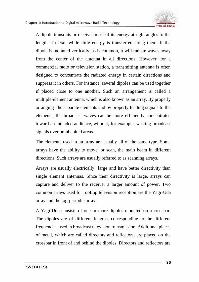
A dipole transmits or receives most of its energy at right angles to the
lengths f metal, while little energy is transferred along them. If the
dipole is mounted vertically, as is common, it will radiate waves away
from the center of the antenna in all directions. However, for a
commercial radio or television station, a transmitting antenna is often
designed to concentrate the radiated energy in certain directions and
suppress it in others. For instance, several dipoles can be used together
if placed close to one another. Such an arrangement is called a
multiple-element antenna, which is also known as an array. By properly
arranging the separate elements and by properly feeding signals to the
elements, the broadcast waves can be more efficiently concentrated
toward an intended audience, without, for example, wasting broadcast
signals over uninhabited areas.
The elements used in an array are usually all of the same type. Some
arrays have the ability to move, or scan, the main beam in different
directions. Such arrays are usually referred to as scanning arrays.
Arrays are usually electrically large and have better directivity than
single element antennas. Since their directivity is large, arrays can
capture and deliver to the receiver a larger amount of power. Two
common arrays used for rooftop television reception are the Yagi-Uda
array and the log-periodic array.
A Yagi-Uda consists of one or more dipoles mounted on a crossbar.
The dipoles are of different lengths, corresponding to the different
frequencies used in broadcast television transmission. Additional pieces
of metal, which are called directors and reflectors, are placed on the
crossbar in front of and behind the dipoles. Directors and reflectors are
Chapter 1: Introduction to Digital microwave Radio Technology
37 TS53TX11St
not wired into the feed element of the antenna at all but merely reflect
and concentrate radio waves toward the directors.
Yagi-Uda antennas are highly directive, and receiving antennas of this
type are often mounted on rotating towers are basses, so that these
antennas can be turned toward the source of the desired transmission.
Log-periodic arrays look similar to Yagi-Uda arrays, but all of the
elements in a log-periodic array are active dipole elements of different
lengths. The dipoles are carefully spaced to provide signal reception
over a wide range of frequencies.
While the dipole, monopole, microwave dish, horn, Yagi-Uda, and log-
periodic are among the most common types of antennas, many other
designs also exist for communicating at different frequencies.
Submarines traveling underwater can receive coded radio commands
from shore by using extremely low frequency (ELF) radio waves. In
order to receive these signals, a submarine unravels a very long wire
antenna behind as it travels underwater. Television camera crews
broadcasting from locations outside the studio use powerful microwave
transmitter antennas, which can send signals to satellites of directly to
the television station. Amateur, or "ham," radio enthusiasts, who
generally use frequencies between those or AM and FM radio, often
construct their own antennas, customizing them for sending and
receiving signals at desired frequencies.

Chapter 1: Introduction to Digital microwave Radio Technology
38 TS53TX11St
1-17 Generators of Microwave Signals And Noise Effect
1-17-1 Frequency Converters
Introduction
In the previous chapters, we discussed High Power Amplifiers (HPA)
and Low Noise Amplifiers (LAN) and the requirement to maintain a
const
ant
pow
er
(eirp
)
to
the
satell
ite. We must also maintain the correct frequency as allocated by
INTELSAT. The frequency stability is a mandatory requirement and
varies with the particular service. For example, IDR carriers are required
Figure (1-15) Mixer Principle
Chapter 1: Introduction to Digital microwave Radio Technology
39 TS53TX11St
to remain within ±3.5KHz of the allocated frequency but SCPC/QPSK
carriers are required to remain within ±250Hz of the allocated
frequency. In order to achieve these limits the Up converter on the
transmit side and the Down converter on the receive side are very
important. This chapter discusses the principles of UP/DOWN
Conversion.
Frequency Conversion Principle
The key for the frequency conversion is the mixer, it is used to obtain
frequencies which are the sums and differences of two input
frequencies (see Figure1-16). in the mixer, the two mixed signals exist
simultaneously in nonlinear devices (diodes). The non-linearity
produces signals with the desired sum of difference of frequencies, but
it also produces many other signals, which can cause problems.
To understand which frequencies are produced lets consider the
following sine waves.
L(t) = A cos (t + ) and; S(t) = B cos (t + ) .
Where : L(t) = Local oscillator signal.
S(t) = Signal to be frequency converted.
= represents the instantaneous phase.
If both signals interacts in a non-linear device as the mixer is, the mixer
output R(t) will be:
R(t) = Km.L(t).S(t) or (
.1)

Chapter 1: Introduction to Digital microwave Radio Technology
40 TS53TX11St
R(t) = Km [ A cos {t + }] [ B cos {t + }] (
.2)
Using the identity
)]cos()[cos(2
1coscos yxyxyx ( .3)
equation (.2) can be expanded to:
R(t) = Km[½A cos {(t + t) + + }] +
Km[½ BA cos {(t - t) - - }] ( .4)
Where : Km = Mixer gain.
The waveform R(t) has its spectrum shifted to the two center
frequencies, {t + t} and {t - t}. A band pass filter following
the mixer can be tuned to select either the sum or the difference of the
mixer output. Hence the input spectrum can be Up-converted to the
sum frequency, or down-converted to the difference frequency.
It is still important to recognize the importance of stability of the
master oscillator. Offsets in the oscillator produce offsets in the output
frequency. Phase variations on the local oscillator such as phase noise
variations, are transferred directly to the translated RF carrier. Theses
effects become important, since they can cause phase and frequency
errors to permeate the entire system.
Frequency converters
1- Single conversion
a- Up Converter

Chapter 1: Introduction to Digital microwave Radio Technology
41 TS53TX11St
By using the described principle, the up-converter (U/C) translate the
intermediate frequency (IF) signal into a radio frequency (RF) signal
(e.g., in the 6GHz or 14GHz band). Conversely, the down-converter
(D/C) translate the RF signal (e.g., in the 4GHz or 11-12GHz band)
into an IF signal
Let us take an example of a " single " mixing technique for Up
Conversion:
f1 = 70MHz intermediate frequency
f2 = 6250MHz mixing frequency
f3 = 6320MHz wanted output frequency
Chapter 1: Introduction to Digital microwave Radio Technology
42 TS53TX11St
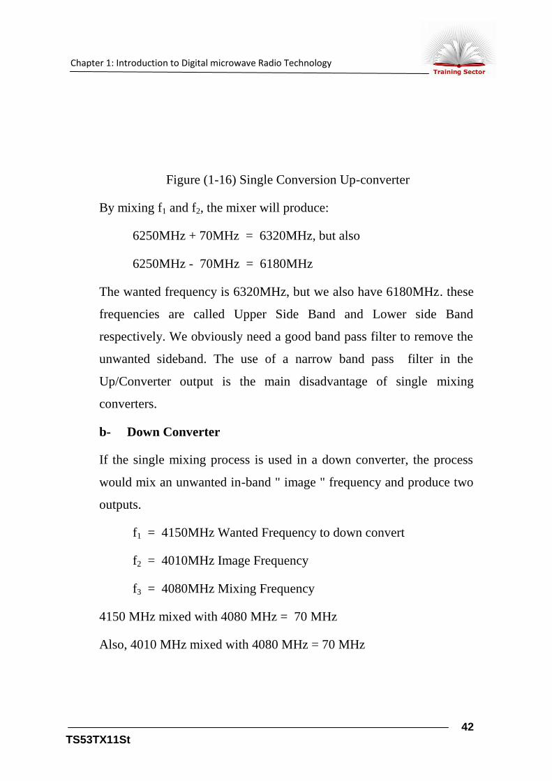
Figure (1-16) Single Conversion Up-converter
By mixing f1 and f2, the mixer will produce:
6250MHz + 70MHz = 6320MHz, but also
6250MHz - 70MHz = 6180MHz
The wanted frequency is 6320MHz, but we also have 6180MHz. these
frequencies are called Upper Side Band and Lower side Band
respectively. We obviously need a good band pass filter to remove the
unwanted sideband. The use of a narrow band pass filter in the
Up/Converter output is the main disadvantage of single mixing
converters.
b- Down Converter
If the single mixing process is used in a down converter, the process
would mix an unwanted in-band " image " frequency and produce two
outputs.
f1 = 4150MHz Wanted Frequency to down convert
f2 = 4010MHz Image Frequency
f3 = 4080MHz Mixing Frequency
4150 MHz mixed with 4080 MHz = 70 MHz
Also, 4010 MHz mixed with 4080 MHz = 70 MHz

Chapter 1: Introduction to Digital microwave Radio Technology
43 TS53TX11St
This shows that incoming 4150 MHz and 4010 MHz will give the same
70 MHz output.
Figure (1-17) Single Conversion Down-converter
Therefore, a band pass filer must be inserted at the input to reject 4080
MHz. it can be seen from the examples that two bands of frequencies
are produced:
a. The wanted band
b. The unwanted band
The tunable filers require a sharp band pass characteristic and can take
up to a few hours to re-tune, which means that a set of filers with
tuning equipment has to be kept on site. To eliminate this problem a
broadband converter design using a double mixing techniques to
operate across the total 500MHz band without the need for filter re-
tuning is normally used in most earth stations.
Requirements
Before describing the double mixing Up/Down Converter we need to
look at the total requirements.

Chapter 1: Introduction to Digital microwave Radio Technology
44 TS53TX11St
It the RF signal bandwidth is relatively narrow, as is the case for
36MHz bandwidth transponders, the intermediate frequency (IF) can be
the conventional 70MHz frequency. However, if wideband RF signals
are used, a higher intermediate frequency must be chosen in order to
improve the filtering of the unwanted signals in the " image " frequency
band. A 140MHz IF is usually
selected. This is the case for transmission and reception of 120Mbit/s
TDMA-PSK signals. It is also the case, for example, for IDR.
2- Double conversion
a-Up/Down Converters
Up and down-converters are usually composed of:
- an RF filter;
- two cascaded mixers.
- two local oscillators (LO); one fixed frequency and the other
variable frequency.
- IF amplifiers(s), possibly with automatic gain control;
- IF filters;
- Group delay equalizer(s) (GDE).
The main performance characteristics of the double up-converters, and
down-converters.
(i) Bandwidth
The RF bandwidth, which defines the capability of the converter
to cover the operational RF band, i.e., to transmit (or receive), by

Chapter 1: Introduction to Digital microwave Radio Technology
45 TS53TX11St
adjusting the LO's frequency to cover the full RF bandwidth
(about 575 Mhz).
The IF bandwidth depends on which IF frequency is selected. If
the IF is 70MHz, the bandwidth will be 36MHz. with an IF of
140MHz the bandwidth will be 72MHz. with this type of
converters, all the carriers of an entire transponder can be Up or
Down converted, this means that every carrier will have different
center frequency, and therefore the carrier frequency tuning and
carrier i.f. filtering will take place in the modem.
Figure (1-18) Double Conversion Up-converter

Chapter 1: Introduction to Digital microwave Radio Technology
46 TS53TX11St
Figure (1-19) Double Conversion Down-converter
(ii) Frequency agility
The frequency may be changed due to changes in the frequency
plan to accommodate traffic increments or when changing to a
new satellite. Therefore, up and down converters which can be
readily adjusted in frequency over the whole RF bandwidth are
required to make these changes. Variable frequency synthesized
local oscillators are used to meet the frequency change
requirements. As explained below, frequency agility (i.e. the
ability to change the RF carrier frequencies) is improved by the
use of double conversion U/C's and D/C's, without the constrain
of filters tuning.
(iii) Equalization
The amplitude-frequency response and group delay of the
transmit and receive sections of earth stations are equalized in
their respective IF sections. (The group delay of satellite

Chapter 1: Introduction to Digital microwave Radio Technology
47 TS53TX11St
transponders are usually equalized in the IF section of the
frequency up converter).
(iv) Linearity
In IDR, IBS and SCPC systems (including the INTELSAT
DAMA system), a number of carriers are frequency converted by
one up or down converter, and intermodulation between carriers
can occur. In the transmit section unit, it is necessary to keep
these unwanted intermodulation products negligibly small
compared to those in the HPA. Therefore, the up converter is
required to have good linearity. For a carrier with a large
bandwidth, good linearity is also necessary to decrease distortion
noise caused by the parabolic component of the delay equalizer
IF section for the whole system as well as to prevent AM-PM
conversion occurring in the converter.
(v) Carrier frequency tolerance
The RF frequency tolerance (i.e: the maximum uncertainty of
initial frequency adjustment plus long-term drift) for the
transmission of IDR, IBS and SCPC/QPSK carriers in the
INTELSAT system is specified as:
IDR: ±0.025R ….. Hz. (but always less than ±3.5 KHz).
IBS: ±0.025R ….. Hz. (but always less than ±10 KHz).
Where R is the carrier transmission rate in bit per second.
However, the frequency tolerance for the transmission of SCPC
carriers is much more stringent, ie: ±250Hz. To realize this latter
tolerance, the local oscillator has to use a crystal-controlled
oscillator with a stability of the order of one part in 108.

Chapter 1: Introduction to Digital microwave Radio Technology
48 TS53TX11St
3- Double mixing
a- UP/DOWN
Converters
This type of converter features high frequency agility since
tuning of the first local oscillator (1st LO or RF oscillator) is
sufficient to change the RF frequency in the entire 500MHz
operational RF band. This type of converter is used most often in
modern earth stations. In down-converter the 4GHz receive input
signal passes through a 500MHz microwave filter, and then
enters a mixer (LO1). It is then mixed with a variable oscillator
frequency and converted into the first intermediate frequency
(1st IF). The 1st IF signal passes through a band-pass filter with
a 80MHz bandwidth and is converted into a 140MHz signal at
the output of the 2nd mixer (LO2). In this configuration, by
making the 1st IF frequency higher than the RF bandwidth, the
frequency in the operating band can be changed by only
changing the frequency of (LO1) without the need for readjusting
the filter. Consequently,, combined with a frequency synthesizer,
this type of converter is very attractive, satisfying requirements
for quick frequency change and remote frequency control. It is
also effective as a single stand-by unit for multiple converters.
4- Local oscillators
The local oscillators used in frequency converters can be driven
either by a crystal pilot or by a frequency synthesizer. In the first
case, changing the frequency requires replacement of the crystal
or switching between multiple crystals. In the second case,
changing the frequency can be effected very simply by

Chapter 1: Introduction to Digital microwave Radio Technology
49 TS53TX11St
thumbwheels or even by remote control. The required long term
frequency stability may range from ±10-5
for TV to 3 x 10⁻⁹
for
SCPC, IDR or TDMA.
Local oscillators must feature low frequency noise at baseband
signal frequencies in order to comply with the general
requirements on earth-station equipment noise. It should be
noted that both low frequency noise requirements and frequency
stability requirements are specially stringent in the case of digital
transmission and reception. High performance crystal controlled
oscillators or frequency synthesizers must be used in this case.
Local oscillators are constructed by taking a pure oscillator
carrier and multiplying, dividing or both its output frequency to
all the desired frequencies needed. Oscillators are simple
electronic devices coupled to tune mechanisms via some type of
feedback. Resonances of the tuning circuit allows a sustained
feedback oscillation to occur, producing an output tone at the
resonant frequency. The oscillator tuning circuits commonly
used are the resistance, inductance, capacitance (RLC), crystal
quartz resonator and the atomic resonators.
5- RLC oscillators
RLC circuits are the simplest and easiest to construct and
therefore are the more frequently used oscillators. However
components imperfections and aging often makes it difficult to
set and maintain precise tone frequency over long time intervals.
6- Crystal oscillators

Chapter 1: Introduction to Digital microwave Radio Technology
50 TS53TX11St
Crystal oscillators use the crystal structure itself as a component
of a resonant circuit to produce a sharply tuned resonances and
relatively stable output tones.
7- Atomic oscillators
The common atomic resonator is the cesium beam, which uses a
stream of cesium atoms to interact with a magnetic field so as to
produce an almost perfect oscillator at the specific frequency of
9.152 GHz. Rubidium resonator, using light beams interacting
with rubidium vapor, produce a fixed oscillation at 6.8 GHz.
Atomic oscillators are often inserted as frequency measurement
standards and are used primarily as reference tones for systems
requiring extreme frequency accuracy, such as the primary
reference oscillator in a digital network.
An ideal oscillator produces a pure sinusoidal carrier with fixed
amplitude, frequency and phase. Practical oscillators, however,
produce waveforms with parameters that may vary in time,
owing to temperature changes, component aging, inherent tuning
circuit noise.
Amplitude variations are somewhat tolerable since they can be
easily controlled with an electronic clipper circuit and limiting
amplifiers. More important to a communication system are the
variation in frequency and phase that may appear on an oscillator
output. Although preliminary system design may be based on the
supposition of ideal carriers, the possibility of imperfect
oscillators are the degradation they may produce must severally
be considered.
Frequency offsets

Chapter 1: Introduction to Digital microwave Radio Technology
51 TS53TX11St
Frequency offsets in oscillators are usually specified as a fraction
of the oscillator design frequency this fraction is generally
normalized by a 10-6
factor and stated in units of parts per
million (ppm). An offset of ∆ƒHz in an oscillator designed for
ƒo hz output frequency will therefore be stated as having an
offset of (∆ƒ/ ƒo)106 ppm. This for example, a 5-MHz oscillator,
specified as having a stability of ±2 ppm, will be expected to
produce an output frequency that is within ±2 x 10-6
x 5 x 106 =
±10 Hz of the desired 5 MHz output.
Oscillator frequency offsets are contributed primarily by
frequency uncertainty (inability to set the desired frequency
exactly), frequency drift (long-term variations due to components
changes), and short-term random frequency variations.
Phase noise
All electronic devices introduce random noise fluctuations due to
thermal agitation of electrons, oscillators are not immune to
effects from random noise. The output signal is not pure, but
contains phase/frequency and amplitude perturbations due to
random noise. These noise perturbations appear as modulation
sidebands around the oscillator carrier output.

Chapter 1: Introduction to Digital microwave Radio Technology
52 TS53TX11St
This phase jitter effectively converts the fixed carrier phase of a
ideal oscillator to a randomly varying phase noise process. This
phase noise has a spectrum that is predominantly low frequency,
extending out to about several kilohertz. In general RLC and
VCOs tend to have higher phase-noise than crystal oscillators,
whereas atomic resonators have the lowest phase noise. Phase-
noise will always be of primary concern in angle modulated
systems, since oscillators phase noise will add directly to any
phase modulation placed in the carrier.
Figure(1-20) Continuous single sideband phase noise requirement
The IESS specification, requests that every earth station shall
satisfy the mask shown in Figure (1-21), for carriers less than
2.048 Mbit/s, taken into account that the carrier phase noise to be
measured is the cumulative total caused by all the Up link path,
including. Modem's carrier oscillators, Up Converters and HP
As. Therefore the phase noise must be measured with a test
equipment arrangement as shown in Figure (1-21) in the down

Chapter 1: Introduction to Digital microwave Radio Technology
53 TS53TX11St
link path in is only required to check the down converter
oscillators phase noise.
Although a number of methods are used to measure phase noise,
only those stations equipped with high quality spectrum
analyzers i.e. with resolution bandwidth of 10Hz and video
bandwidth of 1 Hz, can make the measurement.
Figure (1-22), shows the test equipment set up and a typical
appearance of phase noise side band spectrum. It has to be noted
that we are not only measuring phase noise but discrete signals
some hertz away from carrier frequency.
It is very important to make a difference between phase noise
and discrete signals. Both have different origin but both can
cause unwanted phase change in the digital signal.
Figure.(1-21) Equipment Setup for Phase Noise Measurement and Noise
Spectrum
Discrete signals

Chapter 1: Introduction to Digital microwave Radio Technology
54 TS53TX11St
Are caused by lack of filtering of the main AC frequency in the
power supply of every equipment of the chain but special
attention should be paid to HP As, their frequency can be
multiple of either main AC frequency or the internal oscillating
frequency (for pulse width amplitude modulation power
supplies). For every discrete signal it is true that:
Phase Deviation = { 10 Exp (dBc/20)}*57.3 …. Deg
Where dBc is the distance in dB between the carrier and the
measured noise spike.
As clearly can be seen, every noise spike will cause a carrier
deviation. The discrete signals are stated separately and are
quoted as the difference between the carrier level and the spike
level. The IESS specifies that a spurious component at the
fundamental AC line, shall not exceed – 30dBc, and the sum
(added on a power basis) of all others spurious components shall
not exceed-36dBc.
Phase noise
In a determined bandwidth, the carrier phase deviation caused by
the phase noise is very difficult to calculate as an effective phase
deviation. Then, as a tool to evaluate phase noise the single side
band spectral noise density to the carrier level ratio is measured
at a given frequency offset from the carrier and evaluated with
the mandatory mask provided in the IESS. To certify that the
system performance is according to the specification, several
measurement at different frequency offset may be taken.
dbc/Hz

Chapter 1: Introduction to Digital microwave Radio Technology
55 TS53TX11St
As a dimension unit, dBc/Hz is a ratio in dB, between the carrier
center frequency and the noise measured in the side band, at a
certain distance, but measured with a resolution bandwidth of 1
Hz.
A spectrum analyzer with a 1 Hz resolution bandwidth does not
exist, then to evaluate a real measurement that is made with a
resolution bandwidth filter different than 1 Hz, a correction
factors must be used to mathematically reduce the filter
resolution bandwidth to 1 Hz while accounting the spectrum
analyzer peak detector noise response.
Phase Noise effects
The largest problem experienced in satellite communications
systems is local oscillator phase noise degrading the bit error rate
(BER) performance of digital system employing any type of
phase modulation.
In these systems, the combined effects of phase noise on the
local oscillators used in the transmission path cause phase errors
in the received signal which in turn degrades the BER of the
demodulated data. In severe cases large bursts of errors may be
generated which can cause synchronization loss in the digital
equipment, making the service totally unusable.
This problem is more pronounced on low bit rate systems where
the phase noise occupies a large proportion of the wanted signal

Chapter 1: Introduction to Digital microwave Radio Technology
56 TS53TX11St
bandwidth, and consequently has a greater effect on the system
degradation than in higher bit rate systems.
Measuring Phase Noise using a Spectrum Analyzer
A good quality spectrum analyzer can be used to measure phase
noise directly, providing it has a very stable, synthesized, local
oscillator.
In this method the signal under test is connected to the spectrum
analyzer (as seen in Figure. 1-21), tuned to the correct frequency,
and the level of the noise sidebands relative to the carrier peak
measured directly.
Two correction factors have to be applied to the measured noise
level to convert the value to dBc/Hz: one to normalize the power
to a 1 Hz bandwidth, the other to correct for the fact that the
analyzer has been calibrated for sinusoidal signals rather than
noise.
To normalize to a 1 Hz bandwidth the measuered power must
be divided by the noise bandwidth of the filter used to make
the power measurement. A good approximation for noise
bandwidth is 1.2 times the nominal 3dB resolution
bandwidth, e.g. for a resolution bandwidth of 100 Hz the
noise bandwidth is 120 Hz. A more accurate value may be
obtained by measuring the actual response of the filter and
then computing the noise bandwidth, but this can take some
time and is usually not necessary.
The second correction factor compensates for the logarithmic
IF amplifier and the peak detector used within analogue

Chapter 1: Introduction to Digital microwave Radio Technology
57 TS53TX11St
spectrum analyzers, both of which give different results when
measuring noise rather than sinusoidal signals. This
correction factor is 2.5 dB which has to be added to the
measured noise level.
As an example, suppose the analyzer gave a reading of -54.8 dB
using a 100 Hz filter as a ratio between the carrier and the noise
measured at 1 KHz away from the carrier. This value is
converted to dBc/Hz by applying the previous correction factors,
thus
Noise bandwidth of filter = 100 x 1.2 = 120 Hz
Noise ratio in 1 Hz bandwidth = -54.8 – 101og(120) = -75.6
dB
Random noise correction = -75.6 + 2.5 = -73.1
dBc/Hz
Therefore a ratio of -54.8 dB measured in a 100 Hz filter and K
KHz away from carrier is equivalent to a carrier to phase noise
ratio of -73.1 dBc/Hz. (The specification mask for 1 KHz away
from carrier is -70 dBc/Hz) .
To measure the noise level accurately from a plot would be
rather difficult due to the large variation in the noise spikes.
Some form of averaging is therefore required to smooth out the
response of the noise signal. This can be achieved by reducing
the video bandwidth on the spectrum analyzer, but a more
accurate method available in most good quality analyzers is to
use video averaging. With video averaging successive scans are
stored in memory and the average value is then displayed on the
Chapter 1: Introduction to Digital microwave Radio Technology
58 TS53TX11St
screen. A much smoother display is obtained which allows a
better estimate of the noise level to be made.
To perform the whole evaluation of phase noise with the
spectrum analyzer, the frequency span must be incremented by
10 times in every measurement, from center frequency to 100
Hz, to 1 KHz, to 10 KHz and so on, at least three measurements
per frequency span should be taken at 20%, 50% and 100% of
the span, every measurement converted to dBc/Hz, plotted over
semi-logarithmic paper and compared to the mask.
Measurement Limitations
As different plots are taken, it would appear that the phase noise
is going to exceed the specification at offsets less than 70 Hz.
This illustrates one of the main limitations of this measurement
method – it is not possible to measure close-in to the carrier due
to the shape factor of the resolution filter.
The shape factor (or bandwidth selectivity) is defined as the ratio
of the 60 dB and 3 dB bandwidth of the filter and is typically 10.
This means that a filter with a 3 dB bandwidth of 10 Hz will
have a 60 dB bandwidth of 100 Hz. Therefore a measurement
made at a frequency offset close-in to the carrier will be
corrupted by an attenuated version of the carrier itself. This
effect also applies when measuring close to discrete spikes, such
as the 50 Hz components. For this reason it is not recommended
to make measurement at offsets of less than 100 Hz when using a
10 Hz resolution bandwidth filter.
Another limitation is the dynamic range and noise floor of the
spectrum analyzer. It must be able to handle a large amplitude
Chapter 1: Introduction to Digital microwave Radio Technology
59 TS53TX11St
carrier signal and also resolve low level noise components. A
good check is to position the carrier peak at the top of the
display, note the level of the noise sidebands, and then remove
the input signal. The level of the noise floor due to the spectrum
analyzer alone should now be at least 20 dB lower than the noise
sidebands that are to be measured.
Also, the method cannot be used on sources with a large AM
component, which shows up as noise sidebands, or on sources
with a significant amount of drift.
In spite of these limitations the direct spectrum method is very
suitable for making quick checks on the phase noise performance
of sources generally encountered within earth stations such as
synthesized or phase locked oscillators. The main limitation is
the inability to measure close-in to the carrier, but in practice
most problems have been encountered at larger frequency
offsets, typically around 10 KHz.


Chapter 2: VHF/UHF/Microwave Radio Propagation: A Primer for Digital Experimenters
1 TS53TX11St
Chapter 2: VHF/UHF/Microwave Radio Propagation: A Primer
for Digital Experimenters
Aim of study
Estimating Path Loss,how to measure the loss in a transmission link.
Contents Pages
2.1 Abstract 3
2.2 Introduction 3
2.3 Estimating Path Loss 5
2.4 Free Space Propagation 6
2.5 Conclusions 33
2.6 Acknowledgements 34

Chapter 2: VHF/UHF/Microwave Radio Propagation: A Primer for Digital Experimenters
2 TS53TX11St
Chapter 2
VHF/UHF/Microwave Radio Propagation: A Primer for
Digital Experimenters
2.1 Abstract
This paper attempts to provide some insight into the nature of radio
propagation in that part of the spectrum (upper VHF to microwave) used by
experimenters for high-speed digital transmission. It begins with the basics of
free space path loss calculations, and then considers the effects of refraction,
diffraction and reflections on the path loss of Line of Sight (LOS) links. The
nature of non-LOS radio links is then examined, and propagation effects other
than path loss which are important in digital transmission are also described.
2.2 Introduction
The nature of packet radio is changing. As access to the Internet becomes
cheaper and faster, and the applications offered on the “net” more and more
enticing, interest in the amateur packet radio network which grew up in the
1980s steadily wanes. To be sure, there are still pockets of interest in some
places, particularly where some infrastructure to support speeds of 9600 bps
or more has been built up, but this has not reversed the trend of declining
interest and participation. Nevertheless, there is still lots of interest in packet
radio out there - it is simply becoming re-focused in different areas. Some
applications which do not require high speed, and can take advantage of the
mobility that packet radio can provide, have found a secure niche - APRS is a
good example. Interest is also high in high-speed wireless transmission which
can match, or preferably exceed, landline modem rates. With a wireless link,
you can have a 24-hour network connection without the need for a dedicated

Chapter 2: VHF/UHF/Microwave Radio Propagation: A Primer for Digital Experimenters
3 TS53TX11St
line, and you may also have the possibility of portable or mobile operation.
Until recently, most people have considered it to be just too difficult to do
high-speed digital. For example, the WA4DSY 56 Kbps RF modem has been
available for ten years now, and yet only a few hundred people at most have
put one on the air. With the new version of the modem introduced last year,
56 Kbps packet radio has edged closer to plug „n play, but in the meantime,
landline modem data rates have moved into the same territory. What has
really sparked interest in high-speed packet radio lately is not the amateur
packet equipment, but the boom in spread spectrum (SS) wireless LAN
(WLAN) hardware which can be used without a licence in some of the ISM
bands. The new WLAN units are typically integrated radio/modem/computer
interfaces which mimic either ethernet interfaces or landline modems, and are
just as easy to set up. Many of them offer speeds which landline modem users
can only dream of. TAPR and others are working on bringing this type of SS
technology into the amateur service, where it can be used on different bands,
and without the Effective Radiated Power (ERP) restrictions which exist for
the unlicenced service. This technology will be the ticket to developing high-
speed wireless LANs and MANs which, using the Internet as a backbone,
could finally realize the dream of a high-performance wide-area AMPRnet
which can support the applications (WWW, audio and video conferencing,
etc.) that get people excited about computer networking these days.
Although the dream as stated above is somewhat controversial, the author
believes it represents the best hope of attracting new people to the hobby,
providing a basis for experimentation and training in state-of the- art wireless
techniques and networking, and, ultimately, retaining spectrum for the
amateur radio service. One problem is that most of the people attracted to
using digital wireless techniques have little or no background in RF. When it
comes to setting up wireless links which will work over some distance, they

Chapter 2: VHF/UHF/Microwave Radio Propagation: A Primer for Digital Experimenters
4 TS53TX11St
tend to lack the necessary knowledge about antennas, transmission lines and,
especially, the subtleties of radio propagation. This paper deals with the latter
area, in the hopes of providing this new crop of digital experimenters with
some tools to help them build wireless links which work.
The main emphasis of this paper is on predicting the path loss of a link, so
that one can approach the installation of the antennas and other RF equipment
with some degree of confidence that the link will work. The focus is on
acquiring a feel for radio propagation, and pointing the way towards
recognizing the alternatives that may exist and the instances in which
experimentation may be fruitful. We‟ll also look at some propagation aspects
which are of particular relevance to digital signaling.
2.3 Estimating Path Loss
The fundamental aim of a radio link is to deliver sufficient signal power to the
receiver at the far end of the link to achieve some performance objective. For
a data transmission system, this objective is usually specified as a minimum
bit error rate (BER). In the receiver demodulator, the BER is a function of the
signal to noise ratio (SNR). At the frequencies under consideration here, the
noise power is often dominated by the internal receiver noise; however, this is
not always the case, especially at the lower (VHF) end of the range. In
addition, the “noise” may also include significant power from interfering
signals, necessitating the delivery of higher signal power to the receiver than
would be the case under more ideal circumstances (i.e., back-to-back through
an attenuator). If the channel contains multipath, this may also have a major
impact on the BER. We will consider multipath in more detail later - for now,
we will focus on predicting the signal power which will be available to the
receiver.

Chapter 2: VHF/UHF/Microwave Radio Propagation: A Primer for Digital Experimenters
5 TS53TX11St
2.4 Free Space Propagation
The benchmark by which we measure the loss in a transmission link is the
loss that would be expected in free space - in other words, the loss that would
occur in a region which is free of all objects that might absorb or reflect radio
energy. This represents the ideal case which we hope to approach in our real
world radio link (in fact, it is possible to have path loss which is less than the
“free space” case, as we shall see later, but it is far more common to fall short
of this goal).
Calculating free space transmission loss is quite simple. Consider a
transmitter with power Pt coupled to an antenna which radiates equally in all
directions (everyone‟s favorite mythical antenna, the isotropic antenna). At a
distance d from the transmitter, the radiated power is distributed uniformly
over an area of 4πd2 (i.e. the surface area of a sphere of radius d), so that the
power flux density is:
(1)
The transmission loss then depends on how much of this power is captured by
the receiving antenna. If the capture area, or effective aperture of this antenna
is Ar, then the power which can be delivered to the receiver (assuming no
mismatch or feedline losses) is simply rr SAP (2)
The free space path loss between isotropic antennas is Pt / Pr. Since we
usually are dealing with frequency rather than wavelength, we can make the
substitution f
c to get 222)
4( dfc
Lp
(3)
This shows the classic square-law dependence of signal level versus distance.
What troubles some people when they see this equation is that the path loss
24d
PS t

Chapter 2: VHF/UHF/Microwave Radio Propagation: A Primer for Digital Experimenters
6 TS53TX11St
also increases as the square of the frequency. Does this mean that the
transmission medium is inherently more lossy at higher frequencies? While it
is true that absorption of RF by various materials (buildings, trees, water
vapor, etc.) tends to increase with frequency, remember we are talking about
“free space” here. The frequency dependence in this case is solely due to the
decreasing effective aperture of the receiving antenna as the frequency
increases. This is intuitively reasonable, since the physical size of a given
antenna type is inversely proportional to frequency. If we double the
frequency, the linear dimensions of the antenna decrease by a factor of one
half, and the capture area by a factor of one-quarter. The antenna therefore
captures only one-quarter of the power flux density at the higher frequency
versus the lower one, and delivers 6 dB less signal to the receiver. However,
in most cases we can easily get this 6 dB back by increasing the effective
aperture, and hence the gain, of the receiving antenna. For example, suppose
we are using a parabolic dish antenna at the lower frequency. When we
double the frequency, instead of allowing the dish to be scaled down in size
so as to produce the same gain as before, we can maintain the same reflector
size. This gives us the same effective aperture as before (assuming that the
feed is properly redesigned for the new frequency, etc.), and 6 dB more gain
(remembering that the gain is with respect to an isotropic or dipole reference
antenna at the same frequency). Thus the free space path loss is now the same
at both frequencies; moreover, if we maintained the same physical aperture at
both ends of the link, we would actually have 6 dB less path loss at the higher
frequency. You can picture this in terms of being able to focus the energy
more tightly at the frequency with the shorter wavelength. It has the added
benefit of providing greater discrimination against multipath - more about this
later.
The free space path loss equation is more usefully expressed logarithmically:
Chapter 2: VHF/UHF/Microwave Radio Propagation: A Primer for Digital Experimenters
7 TS53TX11St
Lp = 32.4 + 20 Log f + 20 log d dB ( f in MHz , d in Km)
(4)
or Lp = 36.6 + 20 Log f = 20 Log d dB ( f in MHz , d in Miles)
(5)
This shows more clearly the relationship between path loss and distance: path
loss increases by 20 dB/decade or 6 dB/octave, so each time you double the
distance, you lose another 6 dB of signal under free space conditions.
Of course, in looking at a real system, we must consider the actual antenna
gains and cable losses in calculating the signal power Pr which is available at
the receiver input:
Pr = Pt – Lp + Gt + Gr – Lt – Lr (6) where Pt = transmitter power output (dBm
or dBW, same units as Pr)
Lp = free space path loss between isotropic antennas (dB)
Gt = transmit antenna gain (dBi)
Gr = receive antenna gain (dBi)
Lt = transmission line loss between transmitter and transmit antenna (dB)
Lr = transmission line loss between receive antenna and receiver input (dB)
A table of transmission line losses for various bands and popular cable types
can be found in the Appendix.
Example 1. Suppose you have a pair of 915 MHz WaveLAN cards, and want
to use them on a 10 km link on which you believe free space path loss
conditions will apply. The transmitter power is 0.25 W, or +24 dBm. You also
have a pair of yagi antennas with 10 dBi gain, and at each end of the link, you
need about 50 ft (15 m) of transmission line to the antenna. Let‟s say you‟re
using LMR-400 coaxial cable, which will give you about 2 dB loss at 915

Chapter 2: VHF/UHF/Microwave Radio Propagation: A Primer for Digital Experimenters
8 TS53TX11St
MHz for each run. Finally, the path loss from equation (6a) is calculated, and
this gives 111.6 dB, which we‟ll round off to 112 dB. The expected signal
power at the receiver is then, from (7):
Pr = 24 – 112 + 10 + 10 – 2 – 2 = - 72 dBm
According to the WaveLAN specifications, the receivers require -78 dBm
signal level in order to deliver a low bit error rate (BER). So, we should be in
good shape, as we have 6 dB of margin over the minimum requirement.
However, this will only be true if the path really is equivalent to the free space
case, and this is a big if! We‟ll look at means of predicting whether the free
space assumption holds in the next section.
Path Loss on Line of Sight Links
The term Line of Sight (LOS) as applied to radio links has a pretty obvious
meaning: the antennas at the ends of the link can “see” each other, at least in a
radio sense. In many cases, radio LOS equates to optical LOS: you‟re at the
location of the antenna at one end of the link, and with the unaided eye or
binoculars, you can see the antenna (or its future site) at the other end of the
link. In other cases, we may still have an LOS path even though we can‟t see
the other end visually. This is because the radio horizon extends beyond the
optical horizon. Radio waves follow slightly curved paths in the atmosphere,
but if there is a direct path between the antennas which doesn‟t pass through
any obstacles, then we still have radio LOS. Does having LOS mean that the
path loss will be equal to the free space case which we have just considered?
In some cases, the answer is yes, but it is definitely not a sure thing. There are
three mechanisms which may cause the path loss to differ from the free space
case:
refraction in the earth‟s atmosphere, which alters the trajectory of radio
waves, and which can change with time.

Chapter 2: VHF/UHF/Microwave Radio Propagation: A Primer for Digital Experimenters
9 TS53TX11St
diffraction effects resulting from objects near the direct path.
reflections from objects, which may be either near or far from the direct
path.
We examine these mechanisms in the next three sections.
Atmospheric Refraction
As mentioned previously, radio waves near the earth‟s surface do not
usually propagate in precisely straight lines, but follow slightly curved
paths. The reason is well-known to VHF/UHF DXers: refraction in the
earth‟s atmosphere. Under normal circumstances, the index of refraction
decreases monotonically with increasing height, which causes the radio
waves emanating from the transmitter to bend slightly downwards towards
the earth‟s surface instead of following a straight line. The effect is more
pronounced at radio frequencies than at the wavelength of visible light, and
the result is that the radio waves can propagate beyond the optical horizon,
with no additional loss other than the free space distance loss. There is a
convenient artifice which is used to account for this phenomenon: when the
path profile is plotted, we reduce the curvature of the earth‟s surface. If we
choose the curvature properly, the paths of the radio waves can be plotted
as straight lines. Under normal conditions, the gradient in refractivity index
is such that real world propagation is equivalent to straight-line propagation
over an earth whose radius is greater than the real one by a factor of 4/3 -
thus the often-heard term “4/3 earth radius” in discussions of terrestrial
propagation. However, this is just an approximation that applies under
typical conditions - as VHF/UHF experimenters well know, unusual
weather conditions can change the refractivity profile dramatically. This
can lead to several different conditions. In super refraction, the rays bend
more than normal and the radio horizon is extended; in extreme cases, it

Chapter 2: VHF/UHF/Microwave Radio Propagation: A Primer for Digital Experimenters
10 TS53TX11St
leads to the phenomenon known as ducting, where the signal can propagate
over enormous distances beyond the normal horizon. This is exciting for
DXers, but of little practical use for people who want to run data links. The
main consequence for digital experimenters is that they may occasionally
experience interference from unexpected sources. A more serious concern
is subrefraction, in which the bending of the rays is less than normal, thus
shortening the radio horizon and reducing the clearance over obstacles
along the path. This may lead to increased path loss, and possibly even an
outage. In commercial radio link planning, the statistical probability of
these events is calculated and allowed for in the link design (distance, path
clearance, fading margin, etc.). We won‟t get into all of the details here;
suffice it to say that reliability of your link will tend to be higher if you
back off the distance from the maximum which is dictated by the normal
radio horizon. Not that you shouldn‟t try and stretch the limits when the
need arises, but a link which has optical clearance is preferable to one
which doesn‟t. It‟s also a good idea to build in some margin to allow for
fading due to unusual propagation situations, and to allow as much
clearance from obstacles along the path as possible. For short-range links,
the effects of refraction can usually be ignored.
Diffraction and Fresnel Zones
Refraction and reflection of radio waves are mechanisms which are fairly
easy to picture, but diffraction is much less intuitive. To understand
diffraction, and radio propagation in general, it is very helpful to have some
feeling for how radio waves behave in an environment which is not strictly
“free space”. Consider Fig.(2-1), in which a wavefront is traveling from left
to right, and encountering an obstacle which absorbs or reflects all of the
incident radio energy. Assume that the incident wavefront is uniform; i.e.,
if we measure the field strength along the line A-A‟, it is the same at all

Chapter 2: VHF/UHF/Microwave Radio Propagation: A Primer for Digital Experimenters
11 TS53TX11St
points. Now, what will be the field strength along a line B-B‟ on the other
side of the obstacle? To quantify this, we provide an axis in which zero
coincides with the top of the obstacle, and negative and positive numbers
denote positions above and below this, respectively (we‟ll define the
parameter used on this axis a bit later). Figure (2-1) Shadowing of Radio
Waves by an Object
Figure (2-1) Shadowing of Radio by an Object

Chapter 2: VHF/UHF/Microwave Radio Propagation: A Primer for Digital Experimenters
12 TS53TX11St
Figure (2-2) Signal Levels on the Far Side of the Shadowing Object
Figure (3-3) Fresnel Zone for a Radio Link

Chapter 2: VHF/UHF/Microwave Radio Propagation: A Primer for Digital Experimenters
13 TS53TX11St
The two-dimensional representation of a Fresnel zone is shown in Fig. (2-3).
The surface of the ellipsoid is defined by the path ACB, which exceeds the
length of the direct path AB by some fixed amount. This amount is n/2,
where n is a positive integer. For the first Fresnel zone, n = 1 and the path
length differs by /2 (i.e., a 180o phase reversal with respect to the direct
path). For most practical purposes, only the first Fresnel zone need be
considered. A radio path has first Fresnel zone clearance if, as shown in Fig.
(3-3), no objects capable of causing significant diffraction penetrate the
corresponding ellipsoid. What does this mean in terms of path loss? Recall
how we constructed the wave front behind an object by vector addition of the
wavelets comprising the wave front in front of the object, and apply this to the
case where we have exactly first Fresnel zone clearance. We wish to find the
strength of the direct path signal after it passes the object. Assuming there is
only one such object near the Fresnel zone, we can look at the resultant wave
front at the destination point B. In terms of the Cornu spiral, the upper half of
the spiral is intact, but part of the lower half is absent, due to blockage by the
object. Since we have exactly first Fresnel clearance, the final vector which
we add to the bottom of the spiral is 180o out of phase with the direct-path
vector - i.e., it is pointing downwards. This means that we have passed the
bottom of the spiral and are on the way back up, and the resultant vector is
near the free space magnitude (a line between X and Y). In fact, it is sufficient
to have 60% of the first Fresnel clearance, since this will still give a resultant
which is very close to the free space value.
In order to quantify diffraction losses, they are usually expressed in terms of a
dimensionless parameter v, given by:
V = 2
d (7) Figure (3-6) Fresnel Zone for a Radio Link
difference in lengths of the straight-line path between the endpoints of the link

Chapter 2: VHF/UHF/Microwave Radio Propagation: A Primer for Digital Experimenters
14 TS53TX11St
and the path which just touches the tip of the diffracting object (see Fig. (2-7),
where ∆d = d1 + d2 - d). By convention, v is positive when the direct path is
blocked (i.e., the obstacle has positive height), and negative when the direct
path has some clearance (“negative height”). When the direct path just grazes
the object, v= 0. This is the parameter shown in Figures (3-1) and (3-2). Since
in this section we are considering LOS paths, this corresponds to specifying
that v ó 0. For first Fresnel zone clearance, we have ∆d = /2, so from
equation (8), v= -1.4. From Figure (3-2), we can see that this is more
clearance than necessary - in fact, we get slightly higher signal level (and path
loss less than the free space value) if we reduce the clearance to v= -1, which
corresponds to ∆d = /4. The v= -1 point is also shown on the Cornu spiral in
Fig. (3-3). Since ∆d = /4, the last vector added to the summation is rotated
90o from the direct-path vector, which brings us to the lowest point on the
spiral. The resultant vector then runs from this point to the upper end of the
spiral at point Y. It‟s easy to see that this vector is a bit longer than the
distance from X to Y, so we have a slight gain (about 1.2 dB) over the free
space case. We can also see how we can back off to 60% of first Fresnel zone
clearance (v≈-0.85) without suffering significant loss. But how do we
calculate whether we have the required clearance? The geometry for Fresnel
zone calculations is shown in Fig. (2-4). Keep in mind that this is only a two-
dimensional representation, but Fresnel zones are three-dimensional. The
same considerations apply when the objects limiting path clearance are to the
side or even above the radio path. Since we are considering LOS paths in this
section, we are dealing only with the “negative height” case, shown in the
lower part of the figure. We will look at the case where h is positive later,
when we consider non-LOS paths. For first Fresnel zone clearance, the
distance h from the nearest point of the obstacle to the direct path must be at
least

Chapter 2: VHF/UHF/Microwave Radio Propagation: A Primer for Digital Experimenters
15 TS53TX11St
21
212dd
ddh
(8)
where d1 and d2 are the distances from the tip of the obstacle to the two
ends of the radio circuit. This formula is an approximation which is not
valid very close to the endpoints of the circuit. For convenience, the
clearance can be expressed in terms of frequency:
)21
21
(3.17
ddf
ddh
(9)
where f is the frequency in GHz, d1 and d2 are in km, and h is in
meters. Or:
)(1.72
21
21
ddf
ddh
(10)
where f is in GHz, d1 and d2 in statu0te miles, and h is in feet.
Figure (2-6) Fresnel Zone for a Radio Link
Figure (2-4) Fresnel Zone Geometry
Chapter 2: VHF/UHF/Microwave Radio Propagation: A Primer for Digital Experimenters
16 TS53TX11St
Example 2. We have a 10 km LOS path over which we wish to establish a
link in the 915 MHz band.
The path profile indicates that the high point on the path is 3 km from one
end, and the direct path clears it by about 18 meters (60 ft.) - do we have
adequate Fresnel zone clearance? From equation (10a), with d1 = 3 km, d2 =
7 km, and f = 0.915 GHz, we have h = 26.2 m for first Fresnel zone
clearance (strictly speaking, h = -26.2 m). A clearance of 18 m is about 70%
of this, so it is sufficient to allow negligible diffraction loss.
Fresnel zone clearance may not seem all that important - after all, we said
previously that for the zero clearance (grazing) case, we have 6 dB of
additional path loss. If necessary, this could be overcome with, for example,
an additional 3 dB of antenna gain at each end of the circuit. Now it‟s time to
confess that the situation depicted in Figures (2-1) and (2-2) is a special case,
known as “knife edge” diffraction. Basically, this means that the top of the
obstacle is small in terms of wavelengths. This is sometimes a reasonable
approximation of an object in the real world, but more often than not, the
obstacle will be rounded (such as a hilltop) or have a large flat surface (like
the top of a building), or otherwise depart from the knife edge assumption. In
such cases, the path loss for the grazing case can be considerably more than 6
dB - in fact, 20 dB would be a better estimate in many cases. So, Fresnel zone
clearance can be pretty important on real-world paths. And, again, keep in
mind that the Fresnel zone is three-dimensional, so clearance must also be
maintained from the sides of buildings, etc. if path loss is to be minimized.
Another point to consider is the effect on Fresnel zone clearance of changes in
atmospheric refraction, as discussed in the last section. We may have
adequate clearance on a longer path under normal conditions (i.e., 4/3 earth
radius), but lose the clearance when unusual refraction conditions prevail. On

Chapter 2: VHF/UHF/Microwave Radio Propagation: A Primer for Digital Experimenters
17 TS53TX11St
longer paths, therefore, it is common in commercial radio links to do the
Fresnel zone analysis on something Figure (2-4) Fresnel Zone Geometry close
to “worst case” rather than typical refraction conditions, but this may be less
of a concern in amateur applications.
Most of the material in this section was based on Ref. [2], which is highly
recommended for further reading.
Ground Reflections
An LOS path may have adequate Fresnel zone clearance, and yet still have a
path loss which differs significantly from free space under normal refraction
conditions. If this is the case, the cause is probably multipath propagation
resulting from reflections (multipath also poses particular problems for digital
transmission systems - we‟ll look at this a bit later, but here we are only
considering path loss).
One common source of reflections is the ground. It tends to be more of a
factor on paths in rural areas; in urban settings, the ground reflection path will
often be blocked by the clutter of buildings, trees, etc. In paths over relatively
smooth ground or bodies of water, however, ground reflections can be a major
determinant of path loss. For any radio link, it is worthwhile to look at the
path profile and see if the ground reflection has the potential to be significant.
It should also be kept in mind that the reflection point is not at the midpoint of
the path unless the antennas are at the same height and the ground is not
sloped in the reflection region - just the remember the old maxim from optics
that the angle of incidence equals the angle of reflection.
Ground reflections can be good news or bad news, but are more often the
latter. In a radio path consisting of a direct path plus a ground-reflected path,
the path loss depends on the relative amplitude and phase relationship of the
signals propagated by the two paths. In extreme cases, where the ground
Chapter 2: VHF/UHF/Microwave Radio Propagation: A Primer for Digital Experimenters
18 TS53TX11St
reflected path has Fresnel clearance and suffers little loss from the reflection
itself (or attenuation from trees, etc.), then its amplitude may approach that of
the direct path. Then, depending on the relative phase shift of the two paths,
we may have an enhancement of up to 6 dB over the direct path alone, or
cancellation resulting in additional path loss of 20 dB or more. If you are
acquainted with Mr. Murphy, you know which to expect! The difference in
path lengths can be estimated from the path profile, and then translated into
wavelengths to give the phase relationship. Then we have to account for the
reflection itself, and this is where things get interesting. The amplitude and
phase of the reflected wave depend on a number of variables, including
conductivity and permittivity of the reflecting surface, frequency, angle of
incidence, and polarization.
It is difficult to summarize the effects of all of the variables which affect
ground reflections, but a typical case is shown in Fig. (2-5) [2]. This particular
figure is for typical ground conditions at 100 MHz, but the same behavior is
seen over a wide range of ground constants and frequencies. Notice that there
is a large difference in reflection amplitudes between horizontal and vertical
polarization (denoted on the curves with “h” and “v”, respectively), and that
vertical polarization in general gives rise to a much smaller reflected wave.
However, the difference is large only for angles of incidence greater than a
few degrees (note that, unlike in optics, in radio transmission the angle of
incidence is normally measured with respect to a tangent to the reflecting
surface rather than a normal to it); in practice, these angles will only occur on
very short paths, or paths with extraordinarily high antennas. For typical
paths, the angle of incidence tends to be of the order of one degree or less -
for example, for a 10 km path over smooth earth with 10 m antenna heights,
the angle of incidence of the ground reflection would only be about 0.11
degrees. In such a case, both polarizations will give reflection amplitudes near

Chapter 2: VHF/UHF/Microwave Radio Propagation: A Primer for Digital Experimenters
19 TS53TX11St
unity (i.e., no reflection loss). Perhaps more surprisingly, there will also be a
phase reversal in both cases. Horizontally-polarized waves always undergo a
phase reversal upon reflection, but for vertically-polarized waves, the phase
change is a function of the angle of incidence and the ground characteristics.
The upshot of all this is that for most paths in which the ground reflection is
significant (and no other reflections are present), there will be very little
difference in performance between horizontal and vertical polarization. For
very short paths, horizontal polarization will generally give rise to a stronger
reflection.
If it turns out that this causes cancellation rather than enhancement, switching
to vertical polarization may provide a solution. In other words, for shorter
paths, it is usually worthwhile to try both polarizations to see which works
better (of course, other factors such as mounting constraints and rejection of
other sources of multipath and interference also enter into the choice of
polarization).
As stated above, for either polarization, as the path gets longer we approach
the case where the ground reflection produces a phase reversal and very little
attenuation. At the same time, the direct and reflected paths are becoming
more nearly equal. The path loss ripples up and down as we increase the
distance, until we reach the point where the path lengths differ by just one-
half

Chapter 2: VHF/UHF/Microwave Radio Propagation: A Primer for Digital Experimenters
20 TS53TX11St
wavelength. Combined with the 180
reflection, this brings the direct and reflected signals into phase, resulting in
an enhancement over the free space path loss (theoretically 6 dB, but this will
seldom be realized in practice).
Thereafter, it‟s all downhill as the distance is further increased, since phase
difference between the two paths approaches in the limit the 180o phase shift
of the ground reflection. It can be shown that, in this region, the received
power follows an inverse fourth-power law as a function of distance instead
of the usual square law (i.e., 12 dB more attenuation when you double the
distance, instead of 6 dB). The distance at which the path loss starts to
increase at the fourth-power rate is reached when the ellipsoid corresponding
to the first Fresnel zone just touches the ground.
Figure (3-5) Typical Ground Reflection Parameters

Chapter 2: VHF/UHF/Microwave Radio Propagation: A Primer for Digital Experimenters
21 TS53TX11St
where h1 and h2 are the antenna heights above the ground reflection point.
For example, for antenna heights of 10 m, at 915 MHz (= 33 cm) we will be
into the fourth-law loss region for links longer than about 1.2 km.
So, for longer-range paths, ground reflections are always bad news. Serious
problems with ground reflections are most commonly encountered with radio
links across bodies of water. Spread spectrum techniques and diversity
antenna arrangements usually can‟t overcome the problems - the solution lies
in siting the antennas (e.g., away from the shore of the body of water) such
that the reflected path is cut off by natural obstacles, while the direct path is
unimpaired. In other cases, it may be possible to adjust the antenna locations
so as to move the reflection point to a rough area of land which scatters the
signal rather than creating a strong specular reflection.
Other Sources of Reflections
Much of what has been said about ground reflections applies to reflections
from other objects as well.
The “ground reflection” on a particular path may be from a building rooftop
rather than the ground itself, but the effect is much the same. On long links,
reflections from objects near the line of the direct path will almost always
cause increased path loss - in essence, you have a permanent “flat fade” over
a very wide bandwidth. Reflections from objects which are well off to the side
of the direct path are a different story, however. This is a frequent occurrence
in urban areas, where the sides of buildings can cause strong reflections. In
such cases, the angle of incidence may be much larger than zero, unlike the
ground reflection case. This means that horizontal and vertical polarization
may behave quite differently - as we saw in Fig. (2-5), vertically polarized
signals tend to produce lower-amplitude reflections than horizontally
polarized signals when the angle of incidence exceeds a few degrees. When
Chapter 2: VHF/UHF/Microwave Radio Propagation: A Primer for Digital Experimenters
22 TS53TX11St
the reflecting surface is vertical, like the side of a building, a signal which is
transmitted with horizontal polarization effectively has vertical polarization as
far as the reflection is concerned. Therefore, horizontal polarization will
generally result in weaker reflections and less multipath than vertical
polarization in these cases. Effects of Rain, Snow and Fog
The loss of LOS paths may sometimes be affected by weather conditions
(other than the refraction effects which have already been mentioned). Rain
and fog (clouds) become a significant source of attenuation only when we get
well into the microwave region. Attenuation from fog only becomes
noticeable (i.e., attenuation of the order of 1 dB or more) above about 30
GHz. Snow is in this category as well. Rain attenuation becomes significant at
around 10 GHz, where a heavy rainfall may cause additional path loss of the
order of 1 dB/km.
Path Loss on Non-Line of Sight Paths
We have spent quite a bit of time looking at LOS paths, and described the
mechanisms which often cause them to have path loss which differs from the
“free space” assumption. We‟ve seen that the path loss isn‟t always easy to
predict. When we have a path which is not LOS, it becomes even more
difficult to predict how well signals will propagate over it. Unfortunately,
non-LOS situations are sometimes unavoidable, particularly in urban areas.
The following sections deal with some of the major factors which must be
considered.
Diffraction Losses
In some special cases, such as diffraction over a single obstacle which can be
modeled as a knife edge, the loss of a non-LOS path can be predicted fairly
readily. In fact, this is the same situation that we saw in Figures 1 and 2, with
the diffraction parameter v.

Chapter 2: VHF/UHF/Microwave Radio Propagation: A Primer for Digital Experimenters
23 TS53TX11St
To get ∆d, measure the straight-line distance between the endpoints of the
link. Then measure the length of the actual path, which includes the two
endpoints and the tip of the knife edge, and take the difference between the
two, the “positive h” case. A good approximation to the knife-edge diffraction
loss in dB can then be calculated from :
L (v) = 6.9 + 20 log [ 12 v + v ]
(11)
Example 3. We want to run a 915 MHz link between two points which are a
straight-line distance of 25 km apart. However, 5 km from one end of the link,
there is a ridge which is 100 meters higher than the two endpoints. Assuming
that the ridge can be modeled as a knife edge, and that the paths from the
endpoints to the top of ridge are LOS with adequate Fresnel zone clearance,
what is the expected path loss? From simple geometry, we find that length of
the path over the ridge is 25,001.25 meters, so that ∆d = 1.25 m. Since =
0.33 m, the parameter v, from (7), is 3.89. Substituting this into (12), we find
that the expected diffraction loss is 24.9 dB. The free space path loss for a 25
km path at 915 MHz is, from equation (4), 119.6 dB, so the total predicted
path loss for this path is 144.5 dB. This is too lossy a path for many WLAN
devices. For example, suppose we are using WaveLAN cards with 13 dBi
gain antennas, which (disregarding feedline losses) brings them up to the
maximum allowable EIRP of +36 dBm. This will produce, at the antenna
terminals at the other end of the link, a received power of (36 - 144.5 + 13) =
-95.5 dBm. This falls well short of the -78 dBm requirement of the WaveLAN
cards. On the other hand, a lower-speed system may be quite usable over this
path. For instance, the FreeWave 115 Kbps modems require only about -108
dBm for reliable operation, which is a comfortable margin below our
predicted signal levels.

Chapter 2: VHF/UHF/Microwave Radio Propagation: A Primer for Digital Experimenters
24 TS53TX11St
To see the effect of operating frequency on diffraction losses, we can repeat
the calculation, this time using 144 MHz, and find the predicted diffraction
loss to be 17.5 dB, or 7.4 dB less than at 915 MHz. At 2.4 GHz, the predicted
loss is 29.0 dB, an increase of 4.1 dB over the 915 MHz case (these
differences are for the diffraction losses only, not the only total path loss).
Unfortunately, the paths which digital experimenters are faced with are
seldom this simple. They will frequently involve diffraction over multiple
rooftops or other obstacles, many of which don‟t resemble knife edges. The
path losses will generally be substantially greater in these cases than predicted
by the single knife edge model. The paths will also often pass through objects
such as trees and wood-frame buildings which are semi-transparent at radio
frequencies. Many models have been developed to try and predict path losses
in these more complex cases. The most successful are those which deal with
restricted scenarios rather than trying to cover all of the possibilities. One
Figure (3-6) Diffraction by a Rounded Obstacle

Chapter 2: VHF/UHF/Microwave Radio Propagation: A Primer for Digital Experimenters
25 TS53TX11St
common scenario is diffraction over a single obstacle which is too rounded to
be considered a knife edge. There are different ways of treating this problem;
the one described here is from Ref. [3]. The top of the object is modeled as a
cylinder of radius r, as shown in Fig. (3-6). To calculate the loss, you need to
plot the profile of the actual object, and then draw straight lines from the link
endpoints such that they just graze the highest part of the object as seen from
their individual perspectives. Then the parameters Ds, d1, d2 and
estimated, and an estimate of the radius r can then be calculated from
)(
22
2
2
1
21
dd
ddDr s
(12)
Note that the angle is measured in radians. The procedure then is to
calculate the knife edge diffraction loss for this path as outlined above, and
then add to it an excess loss factor Lex, calculated from
rLex 7.11 (13)
Figure (3-9) Diffraction by a Rounded Obstacle
There is also a correction factor for roughness: if the object is, for example, a
hill which is tree-covered rather than smooth at the top, the excess diffraction
loss is said to be about 65% of that predicted in (13). In general, smoother
objects produce greater diffraction losses. Example 4. We revisit the scenario
in Example 3, but let‟s suppose that we‟ve now decided that the ridge
blocking our path doesn‟t cut it as a knife edge (ouch!). From a plot of the
profile, we estimate that Ds = 10 meters. As before, d1 = 20 km, d2 = 5 km
and the height of the ridge is 100 meters. Dusting off our high school
trigonometry, we can work out that = 1.43o, or 0.025 radians. Now,

Chapter 2: VHF/UHF/Microwave Radio Propagation: A Primer for Digital Experimenters
26 TS53TX11St
plugging these numbers into (12), we get r = 188 meters. Then, with = 0.33
m, we can calculate the excess loss from (13):
So, summed with the knife edge loss calculated previously, we have an
estimated total diffraction loss of 37.3 dB (assuming the ridge is “smooth”
rather than “rough”). This is a lot, but you can easily imagine scenarios where
the losses are much greater: just look at the direct dependence on the angle r
in (13) and picture from Fig. (3-6) what happens when the obstacle is closer
to one of the link endpoints.
Amateurs doing weak signal work are accustomed to dealing with large path
losses in non-LOS propagation, but such losses are usually intolerable in
high-speed digital links.
Attenuation from Trees and Forests
Trees can be a significant source of path loss, and there are a number of
variables involved, such as the specific type of tree, whether it is wet or dry,
and in the case of deciduous trees, whether the leaves are present or not.
Isolated trees are not usually a major problem, but a dense forest is another
story. The attenuation depends on the distance the signal must penetrate
through the forest, and it increases with frequency. According to a CCIR
report [10], the attenuation is of the order of 0.05 dB/m at 200 MHz, 0.1 dB/m
at 500 MHz, 0.2 dB/m at 1 GHz, 0.3 dB/m at 2 GHz and 0.4 dB/m at 3 GHz.
At lower frequencies, the attenuation is somewhat lower for horizontal
polarization than for vertical, but the difference disappears above about 1
GHz. This adds up to a lot of excess path loss if your signal must penetrate
several hundred meters of forest! Fortunately, there is also significant
propagation by diffraction over the treetops, especially if you can get your
antennas up near treetop level or keep them a good distance from the edge of
the forest, so all is not lost if you live near a forest.

Chapter 2: VHF/UHF/Microwave Radio Propagation: A Primer for Digital Experimenters
27 TS53TX11St
General Non-LOS Propagation Models:
There are many more general models and empirical techniques for predicting
non-LOS path losses, but the details are beyond the scope of this paper. Most
of them are aimed at prediction of the paths between elevated base stations
and mobile or portable stations near ground level, and they typically have
restrictions on the frequency range and distances for which they are valid;
thus they may be of limited usefulness in the planning of amateur high-speed
digital links. Nevertheless, they are well worth studying to gain further insight
into the nature of non-LOS propagation. The details are available in many
texts -
Ref. [3] has a particularly good treatment. One crude, but useful,
approximation will be mentioned here: the loss on many non-LOS paths in
urban areas can be modeled quite well by a fourth-power distance law. In
other words, we substitute d4 for d2 in equation (3). In equation (4), we can
substitute 40log(d) for the 20log(d) term, which would correspond to the
assumption of square-law distance loss for distances up to 1 km (or 1 mile, for
the non-metric version of the equation), and fourth-law loss thereafter. This is
probably an overly optimistic assumption for heavily built-up areas, but is at
least a useful starting point.
The propagation losses on non-LOS paths can be discouragingly high,
particularly in urban areas.
Antenna height becomes a critical factor, and getting your antennas up above
rooftop heights will often spell the difference between success and failure.
Due to the great variability of propagation in cluttered urban environments,
accurate path loss predictions can be difficult. If a preliminary analysis of the
path indicates that you are at least in the ballpark (say within 10 or 15 dB) of

Chapter 2: VHF/UHF/Microwave Radio Propagation: A Primer for Digital Experimenters
28 TS53TX11St
having a usable link, then it will generally be worthwhile to give it a try and
hope to be pleasantly surprised (but be prepared to be disappointed!).
Software Tools for Propagation Prediction
Although there is no substitute for experience and acquiring a “feel” for radio
propagation, computer programs can make the job of predicting radio link
performance a lot easier. They are particularly handy for exploring “what if”
scenarios with different paths, antenna heights, etc. Unfortunately, they also
tend to cost money! If you‟re lucky, you may have access to one of the
sophisticated prediction programs which includes the most complex
propagation models, terrain databases, etc. If not, you can still find some free
software utilities that will make it easier to do some of the calculations
discussed above, such as knife edge diffraction losses. One very useful
freeware program which was developed specifically for short-range
VHF/UHF applications is RFProp, by Colin Seymour, G4NNA. Check
Colin‟s Web page at:
http://www.users.dircon.co.uk/~netking/freesw.htm for more information and
downloading instructions.
This is a Windows (3.1, 95 or NT) program which can calculate path loss in
free space and simple diffraction scenarios. In addition to calculating knife
edge diffraction loss, it provides some correction factors for estimating the
loss caused by more rounded objects, such as hills. It also allows changing the
distance loss exponent from square-law to fourth-law (or anything else, for
that matter) to simulate long paths with ground reflections or obstructed urban
paths. There is also some provision for estimating the loss caused when the
signals must penetrate buildings. The program has a graphical user interface
in which the major path parameters can be entered and the result (in terms of

Chapter 2: VHF/UHF/Microwave Radio Propagation: A Primer for Digital Experimenters
29 TS53TX11St
receiver SNR margin) seen immediately. There is also a tabular output which
lists the detailed results along with all of the assumed parameters.
Special Considerations for Digital Systems:
We have previously looked at the effect of multipath on path loss. When
reflections occur from objects which are very close to the direct path, then
paths have very similar lengths and nearly the same time delay. Depending on
the relative phase shifts of the paths, the signals traversing them at a given
frequency can add constructively to provide a gain with respect to a single
path, or destructively to provide a loss. On longer paths in particular, the
effect is usually a loss. Since the path lengths are nearly equal, the loss occurs
over a wide frequency range, producing a “flat” fade.
In many cases, however, reflections from objects well away from the direct
path can give rise to significant multipath. The most common reflectors are
buildings and other manmade structures, but many natural features can also be
good reflectors. In such cases, the propagation delays of the paths from one
end of the link to the other can differ considerably. The extent of this time
spreading of the signal is commonly measured by a parameter known as the
delay spread of the path. One consequence of having a larger delay spread is
that the reinforcement and cancellation effects will now vary more rapidly
with frequency. For example, suppose we have two paths with equal
attenuation and which differ in length by 300 meters, corresponding to a delay
at intervals of 1 MHz, with maxima in between. With a narrowband system,
you may be lucky and be operating at a frequency near a maximum, or you
may be unlucky and be near a null, in which case you lose most of your signal
(techniques such as space diversity reception may help, though). The path loss
in this case is highly frequency-dependent. On the other hand, a wideband

Chapter 2: VHF/UHF/Microwave Radio Propagation: A Primer for Digital Experimenters
30 TS53TX11St
signal which is, say, several MHz wide, would be subject to only partial
cancellation or selective fading. Depending on the nature of the signal and
how information is encoded into it, it may be quite tolerant of having part of
its energy notched out by the multipath channel. Tolerance of multipath-
induced signal cancellation is one of the major benefits of spread spectrum
transmission techniques.
Longer multipath delay spreads have another consequence where digital
signals are concerned, however: overlap of received data symbols with
adjacent symbols, known as intersymbol interference or ISI.
Suppose we try to transmit a 1 Mbps data stream over the two-path
multipath channel mentioned above.
Assuming a modulation scheme with 1 µsec symbol length is used, then the
signals arriving over the two paths will be offset by exactly one symbol
period. Each received symbol arriving over the shorter path will be overlaid
by a copy of the previous symbol from the longer path, making it impossible
to decode with standard demodulation techniques. This problem can be solved
by using an adaptive equalizer in the receiver, but this level of sophistication
is not commonly found in amateur or WLAN modems (but it will certainly
become more common as speeds continue to increase). Another way to attack
this problem is to increase the symbol length while maintaining a high bit rate
by using a multicarrier modulation scheme such as OFDM (Orthogonal
Frequency Division Multiplex), but again, such techniques are seldom found
in the wireless modem equipment available to hobbyists. For unequalized
multipath channels, the delay spread must be much less than the symbol
length, or the link performance will suffer greatly. The effect of multipath-
induced ISI is to establish an irreducible error rate - beyond a certain point,
increasing transmitter power will cause no improvement in BER, since the

Chapter 2: VHF/UHF/Microwave Radio Propagation: A Primer for Digital Experimenters
31 TS53TX11St
BER vs Eb/N0 curve has gone flat. A common rule of thumb prescribes that
the multipath delay spread should be no more than about 10% of the symbol
length. This will generally keep the irreducible error rate down to the order of
10-3 or less.
Thus, in our two-path example above, a system running at 100K symbols/s or
less may work satisfactorily. The actual raw BER requirements for a
particular system will of course depend on the error-control coding technique
used.
Delay spreads of several microseconds are not uncommon, especially in urban
areas. Mountainous areas can produce much longer delay spreads, sometimes
tens of microseconds. This spells big trouble for doing high-speed data
transmission in these areas. The best way to mitigate multipath in these
situations is to use highly directional antennas, preferably at both ends of the
link. The higher the data rate, the more critical it becomes to use high-gain
antennas. This is one advantage to going higher in frequency.
The delay spread for a given link will usually not exhibit much frequency
dependence - for example, there will be similar amounts of multipath whether
you operate at 450 MHz or 2.4 GHz, if you use the same antenna gain and
type. However, you can get more directivity at the higher frequencies, which
often will result in significantly reduced multipath delay spread and hence
lower BER. It may seem strange that high-speed WLAN products are often
supplied with omnidirectional antennas which do nothing to combat
multipath, but this is because the antennas are intended for indoor use. The
attenuation provided by the building structure will usually cause a drastic
reduction in the amplitude of reflections from outside the building, as well as
from distant areas inside the building. Delay spreads therefore tend to be
much smaller inside buildings - typically of the order of 0.1sec or less.

Chapter 2: VHF/UHF/Microwave Radio Propagation: A Primer for Digital Experimenters
32 TS53TX11St
However, as WLAN products with data rates of 10 Mbps and beyond are now
appearing, even delay spreads of this magnitude are problematic and must be
dealt with by such measures as equalizers, high-level modulation schemes and
sectorized antennas.
2.5 Conclusions
Radio propagation is a vast topic, and we‟ve only scratched the surface here.
We haven‟t considered, for example, the interesting area of data transmission
involving mobile stations - maybe next year! Hopefully, this paper has
provided some insight into the problems and solutions associated with setting
up digital links in the VHF to microwave spectrum. To sum up, here are a few
guidelines and principles: Always strive for LOS conditions. Even with LOS,
you must pay attention to details regarding variability of refractivity, Fresnel
zone clearance and avoiding reflections from the ground and other surfaces.
Non-LOS paths will often lead to disappointment unless they are very short,
especially with the high-speed unlicenced WLAN devices. Their low ERP
limits and high receive signal power requirements (due to large noise
bandwidths, high noise figures and sometimes, significant modem
implementation losses) leave little margin for higher-than-LOS path losses.
Hams are not encumbered by the low ERP limits, but it can be very expensive
to overcome excessive path losses with higher transmitter powers.
Use as much antenna gain as is practical. It is always worthwhile to try both
polarizations, but horizontal polarization will often be superior to vertical. It
will generally provide less multipath in urban areas, and may provide lower
path loss in some non-LOS situations (e.g., attenuation from trees at VHF and
lower UHF). Also, interfering signals from pagers and the like tend to be
vertically polarized, so using the opposite polarization can often provide some
protection from them. There are advantages to going higher in frequency, into

Chapter 2: VHF/UHF/Microwave Radio Propagation: A Primer for Digital Experimenters
33 TS53TX11St
the microwave bands, due to the higher antenna gains which can be achieved.
The tighter focusing of energy which can be achieved may result in lower
overall path loss on LOS paths (providing that you can keep the feedline
losses under control), and less multipath. Higher frequencies also have
smaller Fresnel zones, and thus require less clearance over obstacles to avoid
diffraction losses. And, of course, the higher bands have more bandwidth
available for high-speed data, and less probability of interference. However,
the advantage may be lost in non-LOS situations, since diffraction losses, and
attenuation from natural objects such as trees, increase with frequency.
Radio propagation is seldom 100% predictable, and one should never hesitate
to experiment. It‟s very useful, though, to be equipped with enough
knowledge to know what techniques to try, and when there is little probability
of success. This paper was intended to help fill some gaps in that knowledge.
Good luck with your radio links!
2.6 Acknowledgements
The author gratefully acknowledges the work of his daughter Kelly
(http://hydra.carleton.ca/~klm) in producing the figures for this paper.
WaveLAN is a registered trademark of Lucent Technologies, Inc.

Chapter 2: VHF/UHF/Microwave Radio Propagation: A Primer for Digital Experimenters
34 TS53TX11St


Chapter 3: Microwave Antenna Systems
1 TS53TX11St
Chapter 3: Microwave Antenna System
Aim of study
Properties and Definitions of Microwave Antenna Systems and
Applications, Return loss/voltage-standing-wave-ratio (VSWR), Solid
parabolic Microwave Antennas, Flanges, Antenna Options.
Contents pages
3.1 Introduction 2
3.2 Minimizing Interference by antenna design 3
3.3 Microwave Antenna Systems 5
3.4 Properties and Definitions 16
3.5 Return loss / voltage-standing-wave-ratio 18
3.6 Mechanical Design 22
3.7 Mechanical Tests 25
3.8 Solid Parabolic Microwave Antennas 30
3.9 RFS compact line antenna 37
3-10 Solid Parabolic Microwave Antennas 38
3-11 Flanges 42
3-12 EIA Flange Identification 44
3-13 Mounting Information 47
3-14 Antenna Options 50
3-15 Radomes 53

Chapter 3: Microwave Antenna Systems
2 TS53TX11St
Chapter 3
Microwave Antenna Systems
Systems and Applications
3.1 Introduction
Over the past decade microwave links have proven a popular solution for the
telecommunication industry. The relative ease and economy of installation
has been them deployed in an increasing number of point-to-point
applications – from communications backbones (blue), to branch links
(white) and distribution networks (light blue), not to mention applications in
the broadcast industry and private enterprises. With the rise of new cellular
operators and technologies, overall microwave network density is
undeniably escalating. Backbone systems are built country wide in a
majority of case using a ring structure. In the very seldom case that a link is
down the service will remain full operational. The frequencies in use are
below 10 GHz allowing link distances up to 50 km with antennas up to 4.5m
diameter. Branch links are connected to the backbone towers providing the
signal to main areas and towns. The frequencies in use are up to 20 GHz
providing links up to 20 km with medium size antennas. Distribution links
using frequencies above 22 GHz with small antennas are completing the
network. Yet this intensification of microwave communications brings
added challenge. The greater the number of point-to-point links in a given
area, the greater the potential for these to interact with one another and cause
interference. Since any distortion of the signal reduces the quality of service,
controlling interferences is now the mandate of any radio network operator
and national authority. The key issue for consideration is the design and
location of the source of the signal – the antenna .

Chapter 3: Microwave Antenna Systems
3 TS53TX11St
3.2 Minimizing Interference by antenna design
The radiated power of a microwave antenna apart the main beam at 0 deg is
significant up to 90 deg from the main beam. It is these side lobes that can
cause interference with adjacent point-to-point links, and it is theses side
lobes that must be minimized through careful antenna design and installation.
Figure (4-1)

Chapter 3: Microwave Antenna Systems
4 TS53TX11St
RFS is taking care on this fact using advanced antenna designs and extensive
quality control during production. In addition the antenna mounts as well as
fine adjustments means provide an easy and quick antenna installation.
Figure (4-2)

Chapter 3: Microwave Antenna Systems
5 TS53TX11St
3.3 Microwave Antenna Systems
3.3.1 Systems and Applications
a- Radio Link Applications
In the field of telecommunications, recent years have been marked by the
rapid construction of radio link networks for different applications.
b- Radio Link Backbone Systems
Backbone or back haul systems have been built for mobile operators who
want to be independent from Telcos and fixed wire operators. It saves cost for
leasing a fixed line and allows a simple upgrade of the network if higher
capacity is required.
In addition traditional and new telcom's, utilities as well as broadcast
organizations are upgrading their networks to offer higher capacities to clients
or to upgrade their system from analogue to digital service.
Backbone systems usually use large size antennas in frequency bands below
10 GHz. Due to the distance from the antenna to the radio a flexible elliptical
waveguide is used for connection.RFS antennas .
c- Radio link systems for base station connectivity
Mobile operators use microwave in about 70% of cases for the connection of
base station to base station and base station to switching centers. A very quick
and cost effective deployment is mandatory to be successful in a rapidly
growing market.
This construction process is still a long way from completion. The central
issues are higher and more secure network coverage as well as expansion of
capacity. Radio link stations can be erected in a large variety of locations, and

Chapter 3: Microwave Antenna Systems
6 TS53TX11St
these all have specific structural and electrical requirements which must be
fulfilled by the antenna/waveguide system. It is now common practice to
install new base stations on existing radio link towers for backhaul
applications to share the cost of a site. Maximum use is made of existing
infrastructure. The disadvantage in such cases is the high level of radiated
interference caused by existing telecommunication equipment.
These problems can however be overcome by careful frequency planning
together with the use of antennas with high side lobe suppression and high
crosspolarization discrimination.

Chapter 3: Microwave Antenna Systems
7 TS53TX11St
Figure (4-3)

Chapter 3: Microwave Antenna Systems
8 TS53TX11St
Systems and Applications
The number of available radio link towers is no way near enough to
achieve satisfactory network coverage for mobile applications, as the
distance between adjacent towers can be 20 to 50 km depending on the
frequency range in use. For this reason network operators are forced to
use other sites in unusual locations. On account of their height industrial
chimneys can be ideal. However large concentration of emitted gases,
which are caused by turbulence and are potentially highly corrosive, are
encountered in such locations. This means that the antenna system must
be manufactured from corrosion-resistant materials. Furthermore, any
combination of different materials must also be able to resist corrosion.
In urban environments radio links can be installed on multi-story
buildings. This however does not always have a positive effect on the
overall visual impression created by the building. The number of
installation options is restricted, especially if preservation orders have to
be taken into account as well. In such cases the planner's work can be
made easier by incorporating antennas which either blend with the
background or are at least to a large degree inconspicuous.RFS Compact
Line and Lens antennas meet perfectly these requirements offering a
very small shape.

Chapter 3: Microwave Antenna Systems
9 TS53TX11St
A way of reducing the cost for erecting new towers is the use of highvoltage
masts. Large numbers of these masts and pylons already exist and providing
the necessary height. The disadvantage here is that it is not possible to switch-
off the highvoltage supply in order to undertake repairs and maintenance or to
replace the transmission equipment.
It follows therefore that the radio equipment can only be mounted on the mast
at a point below the highvoltage cables. RFS low attenuation FLEXWELL®
Elliptical waveguide can be used for transferring the RF signal to and from
the antenna. In frequency bands above 10 GHz RFS overmoded
FLEXWELL® Elliptical waveguide provides an extremely low attenuation.
This could lead to the use of a smaller antenna size on top of the mast or to a
Figure( 4-4)

Chapter 3: Microwave Antenna Systems
10 TS53TX11St
reduced power of the radio which is enlarging the lifetime of the electronic
equipment. In locations where there is no possibility of installing the antenna
on an existing structure, it will be necessary to erect a new tower. In order to
keep the size and associated costs of the new tower within manageable
proportions, the antennas should offer minimum wind loading while at the
same time assuring high mechanical stability. Simple and fast installation is
also a standard requirement. Especially RFS small and medium size antennas
with their advanced casting mounts meet these requirements perfectly.
Figure (3-5)

Chapter 3: Microwave Antenna Systems
11 TS53TX11St
Systems and Applications
a- Antennas with waveguide installation
Small antennas (1 and 2 ft) operating in the frequency range above 10
GHz are, as a rule, connected directly to the transmission equipment.
Special mechanical and electrical matching ensuresthat the RF signal
passes directly into the radio equipment with the minimum loss.
It is not always possible to integrate the antenna and radio equipment
due to structural restrictions at the installation site. In this case, as with
larger antennas,
use is made of flexible waveguide. Long connections lead to increased
losses. These losses can only be offset in the overall link calculations
by using larger antennas or additional amplifier stages in the
transmission equipment.
An alternative solution is the use of overmoded waveguide. The
attenuation with this type of waveguide is particularly low, as it no
longer operates in the singl-moded frequency range.
Figure (3-6)

Chapter 3: Microwave Antenna Systems
12 TS53TX11St
High order modes are suppressed by means of appropriate filter units in
the waveguide connectors.
There are significant advantages to be gained by using overmoded
waveguide whenever a frequency range above 18 GHz is used in a
mobile communication network.
b- RFS end-to-end philosophy
RFS offers for all installation scenarios the right products:
c- Radio integrated with antenna
The radio unit is directly mounted onto the back of the antenna. This is
a very common type of installation providing a quick and cost effective
solution. RFS is providing a variety of integrated antennas in different
sizes. All interfaces meet highest electrical as well as mechanical
specification to secure a stable operation in the field. Please contact
RFS for more detail.
d- Radio near to the antenna
In cases where the radio can not be attached directly to the antenna, an
additional section of a Twistflex waveguide provides the connection to
the radio. The radio is installed on the pipe or tower near to the
antenna. Twistflex waveguides are also used to connect antennas to
waveguide runs providing the necessary flexibility during installation.
RFS provides Twistflex waveguides in all frequency bands with
different lengths. Necessary fixing hardware can be ordered separately.

Chapter 3: Microwave Antenna Systems
13 TS53TX11St
Figure (3-7)

Chapter 3: Microwave Antenna Systems
14 TS53TX11St
Figure (3-8)
Figure (3-9)

Chapter 3: Microwave Antenna Systems
15 TS53TX11St
Systems and Applications
a- Radio in a shelter
In traditional backbone systems as well as in configurations where
quick and easy maintenance is required, the radio is installed in a
shelter at ground level. In such cases FLEXWELL® Elliptical
Waveguide provides a low-loss connection to the antenna. RFS is
providing all necessary tools and accessories to install the
antenna/waveguide system with best electrical and mechanical
performance. This includes hoisting stockings, flanging tools, bending
tools and fast earthing components.
As waveguide runs have to be filled with dry air, suitable equipment for
manual as well as automatic dehydration is part of the RFS product
portfolio.
b- The bottom line
RFS antenna/waveguide systems provide a high mechanical stability
and corrosion resistance and are easy to install. Antennas and
waveguides are matched offering highest system performance and
stability.
Mechanical features are outstanding to secure the radio link even under
severe environmental conditions.
Small size antennas are offered with a very small shape to minimize the
environmental impact. This is required in rural areas to get the
permission for a radio link much easier.
Electrical characteristics comply and even exceed with national and
international standards to minimize interference and to simplify
network planning.

Chapter 3: Microwave Antenna Systems
16 TS53TX11St
Low-Loss waveguides and simple means of dehydrating short
waveguide runs make planning and maintenance easier.
Optimized logistic and state-of-the-art manufacturing respond to the
request for short delivery times.
3.4 Properties and Definitions
Half Power Beam Width (HPBW) The angle, relative to the main beam
axis, between the two directions at which the co-polar pattern is 3 dB below
Chapter 3: Microwave Antenna Systems
17 TS53TX11St
the value on the main beam axis. The values are nominal and stated as the
minimum for the frequency band.
3.4.1 Gain
The ratio of the radiation intensity, in the main beam axis to the radiation
intensity that would be obtained if the power accepted by the antenna were
radiated isotropically. Value measured in dBi. The values are stated for the
three frequencies at mid-band as well as at bottom and top of the frequency
band. The tolerance for antenna gain is ± 0.2 dB for single polarized antennas.
In the case of dual polarized antennas, tolerance is also ± 0.2 dB for the
average value of both ports and ± 0.3 dB for each port alone.
3.4.2 Front-to-back-ratio (F/B)
Denotes the highest level of radiation relative to the main beam in an angular
zone of 180° ± 40° for all antennas. Tolerance on stated values is 2 dB.
3.4.3 Cross-polar discrimination (XPD)
The difference in dB between the co-polarized main beam gain and the cross-
polarized signal measured within an angular zone in azimuth of twice the
maximum half power beam width of the frequency band. The value is 30 dB
minimum for all antennas except where noted.
3.4.4 Antenna inter-port isolation (IPI)
Denotes the ratio in dB of the power level applied to one port of a dual
polarized antenna to the power level received in the other input port of the

Chapter 3: Microwave Antenna Systems
18 TS53TX11St
same antenna. The value is 35 dB minimum for all antennas (40 dB
respectively 45 dB for UXA antennas).
3.5 Return loss / voltage-standing-wave-ratio (VSWR)
The stated values are guaranteed across the frequency band of operation.
3.5.1 Radiation pattern
A diagram relating power flux density at a constant distance from an antenna
to direction relative to the antenna main beam axis.
Figure (3-11)
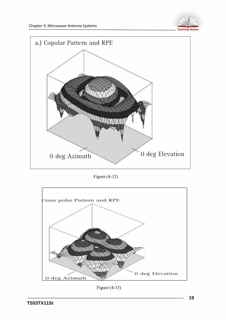
Chapter 3: Microwave Antenna Systems
19 TS53TX11St
Figure (4-13)
Figure (4-12)

Chapter 3: Microwave Antenna Systems
20 TS53TX11St
Properties and Definitions
a- Radiation pattern envelopes (RPE’s)
The envelope represent the worst values of measurements taken on the
pattern test range at the three frequencies mid-band, bottom and top of
the band, in both copolar and cross polar condition, horizontal and
vertical polarized, over the full 360° of azimuth. Since the envelope is
drawn over the highest peaks out of all measurements actual interference
radiation in an operation system will be generally smaller than calculated
from the RPE. Tolerance on given values is 3 dB in an angular region of
±100° and 2 dB from 100° to 180°.
b- Mechanical Properties and Definitions
In addition to the electrical performance RFS designs antennas with
outstanding mechanical features. This assures a high link stability as well
as a long lifetime. Key mechanical features are Survival and Operational
windspeed.
c- Survival windspeed
The antenna sub-system will survive the specified survival windspeed
without any permanent deformation or changes of shape. The value is
250 km/h (70 m/sec) for the 1 ft and 2 ft antennas and 200 km/h (56
m/sec) for all other antennas. An additional load of an ice layer of 30
mm radial ice is taken into account. Special ‘Windload kits’ are available
to improve the survival windspeed of all antennas up to 250 km/h.

Chapter 3: Microwave Antenna Systems
21 TS53TX11St
D- Operational windspeed
The antenna axis deflection is less than one third the half power beam
width at the highest frequency which occurs. The drop in signal is only
approximately 1 dB; the radio link will therefore continue to operate.
The value is 190 km/h (53 m/sec) for all antennas. Antennas with
windload kit offer an operational windspeed of 200 km/h all types.

Chapter 3: Microwave Antenna Systems
22 TS53TX11St
3.6 Mechanical Design
All RFS designs are based on advanced methods of calculation (Finite
Element Method) providing state of the art results. In addition there are
numerous possibilities for simulation based on recognized standards and
regulations. Results have been approved by independent stress analysts. The
proof of mechanical stability is determined on the basis of EIA Standards RS-
195-* and RS-222-* which are recognized world-wide.
* Current Version These standards prescribe the wind resistance coeffi
coefficients (Cw values) to be used for calculating the equivalent forces
caused by wind loading. The values are the result of numerous trials in a
wind tunnel and calculations of aerodynamic properties. Amongst other
things they also take into account the physical shape of the antenna, e.g.
Figure (4-15)

Chapter 3: Microwave Antenna Systems
23 TS53TX11St
reflector only (standard antenna) or reflector with shroud and radome (high
performance antenna).
A wind force Fwind acting on the antenna leads to a load on the mounting
pipe. This load can be divided into an axial force FAT, a lateral force FST
and a torque (turning moment) Mt.
Figure (4-16)

Chapter 3: Microwave Antenna Systems
24 TS53TX11St
Figure (4-17)
Figure (4-18)

Chapter 3: Microwave Antenna Systems
25 TS53TX11St
3.7 Mechanical Tests
In addition to calculation RFS has proven the design with extensive physical
testing. Small size antennas have been put on a shock and vibration test
facility. The applied test conditions exceed the requirement of the European
standard EN 300 019, class 4M5. Wind tunnel tests including 4 ft (1.2m)
antennas and equivalent windload tests complete the mechanical testing.
Windspeeds have been applied exceeding the mechanical design wind speeds
to prove the design even under extreme conditions.
Figure (4-19)
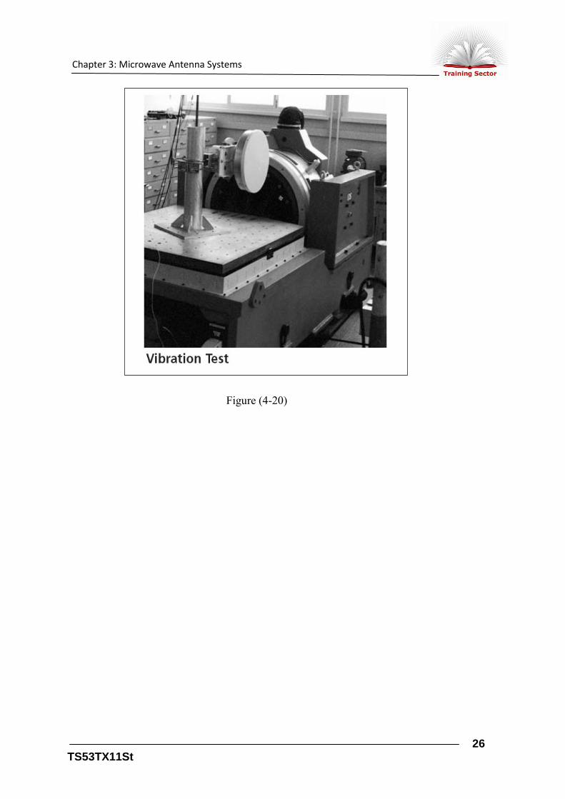
Chapter 3: Microwave Antenna Systems
26 TS53TX11St
Figure (4-20)

Chapter 3: Microwave Antenna Systems
27 TS53TX11St
Figure (3-21)

Chapter 3: Microwave Antenna Systems
28 TS53TX11St
Mechanical Tests
Large size antennas are difficult to be tested in a standard wind tunnel
due to a missing rigid mounting structure. Therefore RFS has designed
an equivalent windload test rig. The job of the test rig is to apply
different forces to the antenna in such a way that it simulates the wind
force, split into an axial component Fa, a lateral component Fs and the
torque Mv that develops in the vertex of the antenna. For this purpose
the test rig has different independent hydraulic systems, which employ
hydraulic cylinders and a band to apply forces to the antenna. The
contour of the antenna is checked with a template before and after the
load is applied. According to the definition of survival windspeed no
Figure (4-22)

Chapter 3: Microwave Antenna Systems
29 TS53TX11St
permanent deformation or changes of shape has to occur on the antenna
sub-system. Dial gauges register the flexible change of shape of the
antenna and the mast mounting during the test. This system enables
antennas with a diameter of up to 4.5 m to be measured at a wind load
of up to 250 km/h. Forces acting on the mounting pipe can be up to 150
kN axially and 40 kN laterally, together with a torque of 90 kNm. The
hydraulic pressure required to create these measurement conditions is
approx. 65 bar.
Bottom Line: RFS antennas provide secure operations under all
standard environmental conditions. This is assured by the use of
corrosion resistant materials as well as selected material combinations.
Continuous proving in environmental chambers and salt fog spray test
facilities guarantee an outstanding long lifetime.
Figure (4-23)

Chapter 3: Microwave Antenna Systems
30 TS53TX11St
3.8 Solid Parabolic Microwave Antennas
3.8.1 Introduction and Antenna Descriptions
Radio Frequency Systems offers the most comprehensive line of highest
quality microwave antennas in the industry. Antennas are available in all the
common frequency bands ranging from 3GHz to 60GHz. They are available
in diameters from 1 ft (0.3 m) to 15 ft (4.60 m). System design becomes easy
and efficient with such a comprehensive antenna offering.
The antennas are available in four performance classes offering complete
flexibility when designing a network. The antennas meet the pattern
requirements according to EN 300 631, EN 300 833 and FCC depending on
the frequency range. In addition to the different electrical classes of antennas
Radio Frequency Systems offers the system design engineers different options
of survival wind speeds. This allows the use of antennas in areas where
extreme wind conditions are normal.
3.8.2 Standard Performance Antennas
Standard Performance Antennas are economical solutions for systems where
side lobe suppression is of less importance. The antennas consist of a
reflector, feed and tower mount. Low VSWR versions are available for low
echo distortion.

Chapter 3: Microwave Antenna Systems
31 TS53TX11St
3.8.3 Improved Performance Antennas
Improved Performance Antennas are unshrouded and offer an economic
solution for systems requiring good radiation performance particularly in the
back region. The improved F/B ratio is achieved by use of an efficient feed
design together with a deep dish reflector. These features result in an
improved front to back ratio, and were specially designed to meet FCC
category A standards.
3.8.4 High Performance Antennas
High Performance Antennas are similar to Ultra High Performance Antennas
in construction. They are ideally suited for systems where a good level of side
lobe suppression is required.
3.8.5 Ultra High Performance Antennas
Ultra High Performance Antennas are the optimum choice for systems where
a high level of pattern performance is required because of high local radio
congestion. The antennas are supplied with low VSWR feed, planar radome,
tower mount and shroud with RF absorber.

Chapter 3: Microwave Antenna Systems
32 TS53TX11St
3.8.6 High Cross Polar Discrimination Antennas
UXA series of antennas are based on Ultra High Performance Antennas.
These antennas offer high side lobe suppression. In addition UXA antennas
offer extremely high cross-polar discrimination. They are therefore ideally
suited for very high capacity systems utilizing extensive frequency reuse in
highly congested environments. This outstanding performance is achieved by
use of a special corrugated illuminator, a rigid torsion box back structure
which ensures the reflector maintains its shape in the field and strict quality
control during manufacture. The cross-polar characteristics for radiation
angles close to bore sight meet the highest XPD requirements according to
EN 300 833 and FCC. High cross-polar discrimination antennas are available
for frequencies from 4 GHz to 23 GHz.

Chapter 3: Microwave Antenna Systems
33 TS53TX11St
3.8.7 Introduction and Antenna Descriptions
Reflectors
Antennas with diameters up to 10ft (3.0m) are supplied with reflectors in one
piece.
Antennas with diameters 12ft (3.7m) are supplied with a two piece reflector
(except UXA-types). Antennas with diameters of 15ft (4.6m) are supplied
with a 3 piece reflector, 8ft and 10ft antennas are available in 2 pieces.
Figure (3-24)
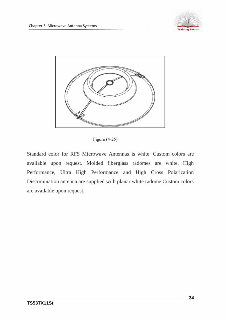
Chapter 3: Microwave Antenna Systems
34 TS53TX11St
Standard color for RFS Microwave Antennas is white. Custom colors are
available upon request. Molded fiberglass radomes are white. High
Performance, Ultra High Performance and High Cross Polarization
Discrimination antenna are supplied with planar white radome Custom colors
are available upon request.
Figure (4-25)

Chapter 3: Microwave Antenna Systems
35 TS53TX11St
3.8.8 Slim Line and Compact Line Antennas
Radio Frequency Systems recognizes that mobile operators and private
microwave users have requirements for cost effective solutions for their
microwave antenna systems. These needs include products, which are easy
and quick to install while maintaining good electrical performance. In
response to these needs Radio Frequency Systems developed the Slim Line
and Compact Line series of antennas.
The Slim Line series of antennas utilize a conventional feed system and are
available in Standard, High and Ultra High performance versions. The Slim
Line series of antennas are available in diameters from 1ft (0.3m) to 6 ft (1.8
m).
Figure (4-26)

Chapter 3: Microwave Antenna Systems
36 TS53TX11St
The Compact Line series of antennas use a special feed system which results
in a reduced shroud length and consequently a lower profile antenna. These
antennas are lighter in weight than standard antennas for reduced tower
loading and shipping costs.
Figure (4-27)

Chapter 3: Microwave Antenna Systems
37 TS53TX11St
Furthermore Compact Line antennas up to 2ft (0.6m) diameter are very
rugged, with a wind loading rating of 250 km/h (155mph). Their type
designation is SB for single polarization and SBX for dual polarization.
Compact Line antennas are available in 1ft (0.3 m), 2 ft (0.6 m), 3ft (0.9 m)
and 4ft (1.2 m) diameters.
3.9 RFS Compact Line Antennas
Single polarized Ultra High Performance SB Dual Polarized Ultra High
Performance SBX 1ft and 2 ft antennas consist of anintegrated
reflector/shroud system avoiding any RF-leakage. This is a further
contribution offering excellent radiation performance especially in the back
direction.
Figure (4-28)

Chapter 3: Microwave Antenna Systems
38 TS53TX11St
1ft and 2 ft antennas consist of an integrated reflector/shroud system
avoiding any RF-leakage. This is a further contribution offering
excellent radiation performance especially in the back direction.
3.10 Solid Parabolic Microwave Antennas
3.10.1 Lens Antennas
RFS lens antennas are an economical solution for short haul radio links. The
antennas are based on conventional horn antenna design. A dielectric lens is
used to correct the phase difference at the aperture, which occurs due to the
large ratio of wavelength to aperture diameter. Lens antennas have no metallic
parts blocking the radiating aperture. This results in a very high antenna
efficiency of nearly 70%.
An additional advantage is the visual impression. To a certain extent a lens
antenna looks like a lamp. This solution is highly suited to installations where
environmental restrictions limit the choice of antenna type, such as in the
proximity of listed buildings or monuments.
Lens antennas are available with a diameter of 0.5ft (0.15m) offering an ultra
high radiation performance.
Figure (4-29)

Chapter 3: Microwave Antenna Systems
39 TS53TX11St
3.10.2 Customized Antennas
RFS Slim Line and especially RFS Compact Line antennas can be provided
with a custom designed adaption for the outdoor unit of the radio equipment.
This allows the outdoor unit of the radio to be mounted directly the antenna,
removing the need for an additional twist flex or elliptical waveguide
connection between the radio and the antenna. The antenna is normally
mounted to a vertical pole. The equipment box can be replaced without the
need for a realignment the antenna system. RFS is taken special care to meet
highest electrical as well as mechanical requirements of the interface. In
Figure (4-30)

Chapter 3: Microwave Antenna Systems
40 TS53TX11St
addition to wind tunnel tests, shock and vibration tests with radios as well as
water spray tests are performed demonstrating a leakage free interface.
RFS is continuously increasing the product portfolio of customized antennas.
For more details please contact RFS.
Figure (4-31)
Figure (3-32)
Figure (4-32)

Chapter 3: Microwave Antenna Systems
41 TS53TX11St
3.10.3 Antenna Types, Overview
3.10.4 Ordering Information & Antenna Options
In order to easily identify an antenna model RFS utilizes a model numbering
system which clearly identifies the antenna type, diameter, frequency,
revision and antenna input.
In addition to the standard products Radio Frequency Systems offers,
products with increased wind rating, improved environmental ratings, planar
radome colors and radome types. For these options please contact your local
RFS sales office.
Figure (3-33)

Chapter 3: Microwave Antenna Systems
42 TS53TX11St
3.11 Flanges
Different flange types are available for the whole antenna range. The flange
sizes, -profiles and dimensions are in accordance with specifications 154 IEC
and EIA (Electronic Industry Association) which classifies the flange types in
the following coding systems:
3.11.1 IEC-flanges
1st digit pressurizable or unpressurizable etc. 2nd digit flange type-A, B, D
etc. 3rd digit waveguide profile, rectangular, etc. secondary numbers
Waveguide size according to 154-IEC.

Chapter 3: Microwave Antenna Systems
43 TS53TX11St
Figure (3-34)

Chapter 3: Microwave Antenna Systems
44 TS53TX11St
3.12 EIA Flange Identification
3.12.1 CPRG Flanges
CPRG, pressurizable contact flanges, are flat faced with a gasket groove and
secured with nuts and bolts. One full thickness gasket is used when mating
two CPRG flanges.
3.12.2 Choke Flanges
Choke flanges include a choke groove, gasket groove and threaded bolt holes
for mating to a cover flange. One O-ring is used when mating a choke flange
to a cover flange without\ gasket groove. Use an O-ring and half gasket when
mating a choke flange to a cover/gasket flange. Two choke flanges cannot be
mated.
Figure (4-35)

Chapter 3: Microwave Antenna Systems
45 TS53TX11St
3.12.3 Cover Flanges
Cover flanges are flat faced without any choke or gasket grooves, and have
clear bolt holes for mating to a choke or cover flange. A conductive gasket is
required when mating two cover flanges. One O-ring is used when mating a
cover flange to a cover/gasket flange.
Figure (3-36)
Figure (4-37)

Chapter 3: Microwave Antenna Systems
46 TS53TX11St
3.12.4 Cover/Gasket
Cover/gasket flanges are flat faced with a gasket groove only, and have clear
bolt holes for mating with a choke, cover, or cover/gasket flange. One O-ring
and a half gasket are used when mating two cover/gasket flanges or when
mating a cover/gasket flange to a choke flange. One O-ring is used when
mating a cover/gasket flange to a cover flange without gasket groove.
Figure (4-38)

Chapter 3: Microwave Antenna Systems
47 TS53TX11St
3.13 Mounting Information
3.13.1 Solid Parabolic Microwave Antennas
Multi-purpose mount (M-mount) for 1 and 2 ft
Antennas The mounting hardware – called the M-mount – has been
especially designed for the installation of small antennas (1 and 2 ft).
The M-mount provides ± 30 deg fine adjustment of both azimuth and
elevation. This is especially important for small antennas used in short
radio links. The mount is made primarily from cast aluminum parts,
which provide outstanding stability together with a very low weight.
The basic material of the mount is seawater-resistant aluminum alloy.

Chapter 3: Microwave Antenna Systems
48 TS53TX11St
The M-mount enables small antennas (1 and 2 ft) to be mounted on
pipe diameters of 48-114 mm (2-4.5 in).
The mount is standard for all 2 ft antennas. It can be ordered optional
for 1 ft antennas.
Oversized Mounting Hardware
The Oversized Mounting Hardware has been specially designed for the
installation of small antennas on larger diameter pipes which are
already in place on radio link towers. These pipes are often larger than
the standard 114 mm. Therefore RFS has designed an alternative
mounting bracket which makes it unnecessary for the installation team
to provide a special mechanical interface. The Oversized Mounting
Hardware enables small antennas to be mounted on pipe diameters of
120-219 mm (4.8-9 in).
The easy and fast installation saves time and cost because no additional
steel work has to be prepared.
In addition the Oversized Mounting Hardware provides more flexibility
and higher stability to secure the link.
For more details contact RFS.

Chapter 3: Microwave Antenna Systems
49 TS53TX11St
Figure (4-39)
Figure (3-40)

Chapter 3: Microwave Antenna Systems
50 TS53TX11St
3.14 Antenna Options
3.14.1 Increased Wind Load Kit
Large RFS antennas, 6 to 12 ft (1.8 to 3.7m) diameter, already incorporate a
strong back ring structure to support the reflector. The hot dip galvanized
steel mount is fixed to the back ring. This configuration allows a simple
upgrade of one of the antenna’s most important mechanical features. The
Increased Wind Load Kit consists of additional struts for mounting between
the back ring and the reflector rim. Thus enables the wind forces to be
directed to the most rigid part of the antenna mount.
The 3 and 4 ft antennas can simply be upgraded by an additional side strut
due to basic strong casting mount. The kit can be installed on site before
lifting the antenna onto the tower. Antennas with a wind load kit provide a
survival wind speed of 250 km/h (155mph), 200 km/h (125mph) without kit,
and an operational wind speed of 200 km/h (125mph), 190 km/h (118mph)
without kit.
3.14.2 Sway Bars
For protection against antenna shifting and deflection, 6, 8, 10 and 12 ft (1.8,
2.4, 3.0 and 3.7m) antennas contain one sway bar and 15 ft (4.6m) antennas
have four (4) sway bars. Additional sway bars are available as an option for
all 6ft (1.8 m) to 12ft (3.7m) antennas.
3.14.3 Harsh Environment Antennas
For increased protection within extreme corrosive and humid environments,
harsh environment antennas are offered as an option. These antennas come
with special corrosion resistant components and finishes, and are designed to

Chapter 3: Microwave Antenna Systems
51 TS53TX11St
withstand corrosive weathering environments typical of industrial, shoreline
and offshore environments.
Figure (4-41)
Figure (3-42)

Chapter 3: Microwave Antenna Systems
52 TS53TX11St
Figure (4-42)
Figure (3-43)
Figure (4-44)

Chapter 3: Microwave Antenna Systems
53 TS53TX11St
3.15 Radomes
3.15.1 Solid Parabolic Microwave Antennas
Molded Radomes
Optional molded radomes are available for Standard Performance
antennas 2 to 12 ft. The radomes are made of fiberglass reinforced
polyester resin covered with a gel coat. The 2 ft radome is manufactured
from ABS material. The shape minimizes the influence of the radome
upon antenna gain, return loss and radiation characteristic.
Radomes with a special flat shape are available for all 4 and 6 ft
antennas above 5.6 GHz. These radomes provide reduced packing
volume and therefore are ideal for transportation. The radomes are
identified by 'SH' in the model name. Moulded radomes protect against
the accumulation of snow, ice and dirt, and reduce windload. The surface
is protected against ultraviolet degradation The standard colour is white.

Chapter 3: Microwave Antenna Systems
54 TS53TX11St
Figure (4-45)
Flexible Planar Radomes
Flexible Planar radomes manufactured from Complan are supplied with
all shrouded antennas > 2ft with the exception of 3 and 4 ft
CompactLine antennas. For Teflon coated fiberglass radomes please
contact RFS.
3.15.2 Replacement Planar Radomes
Replacement radomes are available. Please contact RFS.

Chapter 3: Microwave Antenna Systems
55 TS53TX11St
Parabolic Point to Point Antennas 2.3 - 2.5 GHz

Chapter 3: Microwave Antenna Systems
56 TS53TX11St
Figure (3-46)

Chapter 3: Microwave Antenna Systems
57 TS53TX11St
Figure (4-47)

Chapter 3: Microwave Antenna Systems
58 TS53TX11St
Figure (4-48)

Chapter 3: Microwave Antenna Systems
59 TS53TX11St
Figure (4-49)

Chapter 3: Microwave Antenna Systems
60 TS53TX11St
Figure (4-50)

Chapter 3: Microwave Antenna Systems
61 TS53TX11St
Figure (4-51)

Chapter 3: Microwave Antenna Systems
62 TS53TX11St
Figure (4-52)

Chapter 3: Microwave Antenna Systems
63 TS53TX11St
Figure (3-53)

Chapter 3: Microwave Antenna Systems
64 TS53TX11St
Figure (3-54)