A

Project Report

on

Experimental Study on Measuring Diffusion Coefficients of various

Organic Solvents and Solids with varying Geometries in Air

Submitted by

Durga Prasad Moharana

(Roll No: 110CH0079)

In partial fulfillment of the requirements for the degree in

Bachelor of Technology in Chemical Engineering

Under the guidance of

Dr. Pradip Chowdhury

Department of Chemical Engineering

National Institute of Technology Rourkela

May, 2014

ii

CERTIFICATE

This is certified that the work contained in the thesis entitled “Experimental Study on

Measuring Diffusion Coefficients of various Organic Solvents and Solids with varying

Geometries in Air” submitted by Durga Prasad Moharana (110CH0079), has been carried

out under my supervision and this work has not been submitted elsewhere for a degree.

____________________

Date:

Place: (Thesis Supervisor)

Dr. Pradip Chowdhury

Assistant Professor, Department of

Chemical Engineering

NIT Rourkela

iii

Acknowledgements

First and the foremost, I would like to offer my sincere gratitude to my thesis supervisor, Dr.

Pradip Chowdhury for his immense interest and enthusiasm on the project. His technical

prowess and vast knowledge on diverse fields left quite an impression on me. He was always

accessible and worked for hours with me. Although the journey was beset with complexities

but I always found his helping hand. He has been a constant source of inspiration for me.

I am also thankful to all faculties and support staff of Department of Chemical

Engineering, National Institute of Technology Rourkela, for their constant help and extending

the departmental facilities for carrying out my project work.

I would like to extend my sincere thanks to my friends and colleagues. Last but not the least,

I wish to profoundly acknowledge my parents for their constant support.

________________________

(Durga Prasad Moharana)

110CH0079

iv

ABSTRACT

Molecular diffusion is fundamental to mass transport and understanding the basic mechanism

of this phenomenon and quantitative estimation of the same is critical to mass transfer

operations viz. distillation, absorption/stripping, liquid-liquid extraction etc. In this project,

two contrastingly different cases were selected to experimentally measure binary diffusion

coefficients. It is important to highlight the fact that any industrial mass transfer operation

involves multi-component system; however, suitable binary system data can be effectively

used to estimate the multi-component system. Similarly, for any unit operation involving

more than a single-phase (and hence presence of an interphase), it is the local or overall mass

transfer co-efficient which explains the mass transfer operation prevailing within the system

and can be effectively measured in wetted wall column experiments. However, suitably

measured diffusivity data can easily be used in estimating the mass transfer coefficients using

fundamental concepts of various predictive theories like (film, penetration, surface renewal

and boundary layer). In this work, several organic solvents viz. benzene, toluene, acetone,

carbon-tetrachloride were used to measure their diffusion coefficients in air at widely

different temperatures and at atmospheric pressure. Similarly, solids of different geometries

(both spherical as well as cylindrical) were chosen to measure the diffusivity. Naphthalene

balls (C10H8) were used to study the diffusion phenomenon in spherical geometry and

camphor pellets (C10H16O) were used to study the cylindrical system.

v

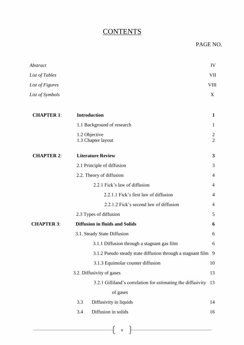
CONTENTS

PAGE NO.

Abstract IV

List of Tables VII

List of Figures VIII

List of Symbols X

CHAPTER 1: Introduction 1

1.1 Background of research 1

1.2 Objective 2

1.3 Chapter layout 2

CHAPTER 2: Literature Review 3

2.1 Principle of diffusion 3

2.2. Theory of diffusion 4

2.2.1 Fick‟s law of diffusion 4

2.2.1.1 Fick‟s first law of diffusion 4

2.2.1.2 Fick‟s second law of diffusion 4

2.3 Types of diffusion 5

CHAPTER 3: Diffusion in fluids and Solids 6

3.1. Steady State Diffusion 6

3.1.1 Diffusion through a stagnant gas film 6

3.1.2 Pseudo steady state diffusion through a stagnant film 9

3.1.3 Equimolar counter diffusion 10

3.2. Diffusivity of gases 13

3.2.1 Gilliland‟s correlation for estimating the diffusivity 13

of gases

3.3 Diffusivity in liquids 14

3.4 Diffusion in solids 16

vi

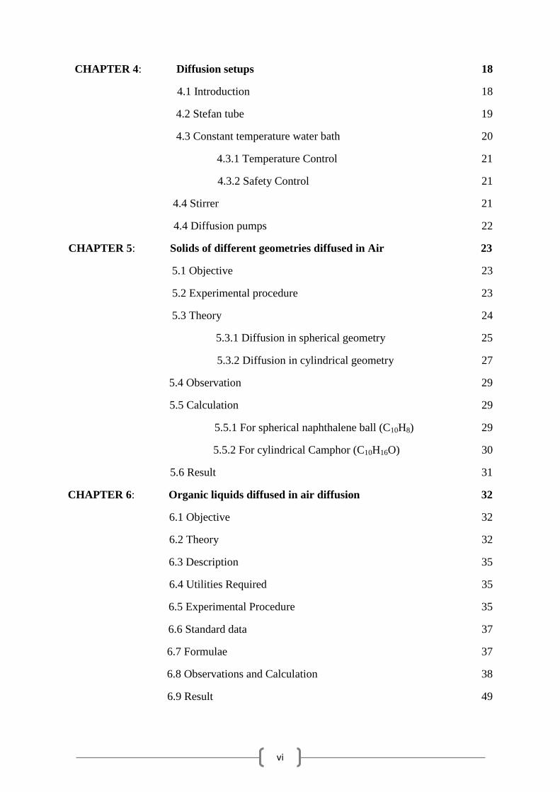
CHAPTER 4: Diffusion setups 18

4.1 Introduction 18

4.2 Stefan tube 19

4.3 Constant temperature water bath 20

4.3.1 Temperature Control 21

4.3.2 Safety Control 21

4.4 Stirrer 21

4.4 Diffusion pumps 22

CHAPTER 5: Solids of different geometries diffused in Air 23

5.1 Objective 23

5.2 Experimental procedure 23

5.3 Theory 24

5.3.1 Diffusion in spherical geometry 25

5.3.2 Diffusion in cylindrical geometry 27

5.4 Observation 29

5.5 Calculation 29

5.5.1 For spherical naphthalene ball (C10H8) 29

5.5.2 For cylindrical Camphor (C10H16O) 30

5.6 Result 31

CHAPTER 6: Organic liquids diffused in air diffusion 32

6.1 Objective 32

6.2 Theory 32

6.3 Description 35

6.4 Utilities Required 35

6.5 Experimental Procedure 35

6.6 Standard data 37

6.7 Formulae 37

6.8 Observations and Calculation 38

6.9 Result 49

vii

CHAPTER 7: Conclusion and Future work 50

References 51

viii

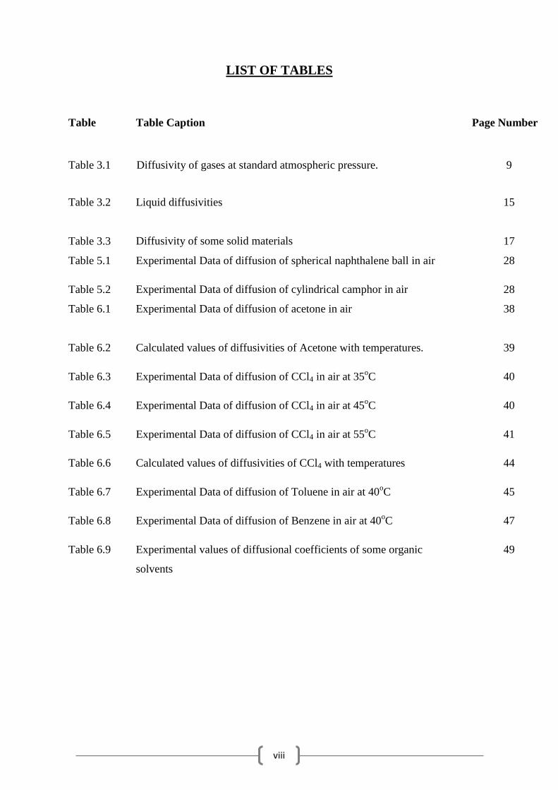
LIST OF TABLES

Table Table Caption Page Number

Table 3.1 Diffusivity of gases at standard atmospheric pressure. 9

Table 3.2 Liquid diffusivities 15

Table 3.3 Diffusivity of some solid materials 17

Table 5.1 Experimental Data of diffusion of spherical naphthalene ball in air 28

Table 5.2 Experimental Data of diffusion of cylindrical camphor in air 28

Table 6.1 Experimental Data of diffusion of acetone in air 38

Table 6.2 Calculated values of diffusivities of Acetone with temperatures. 39

Table 6.3 Experimental Data of diffusion of CCl4 in air at 35oC 40

Table 6.4 Experimental Data of diffusion of CCl4 in air at 45oC 40

Table 6.5 Experimental Data of diffusion of CCl4 in air at 55oC 41

Table 6.6 Calculated values of diffusivities of CCl4 with temperatures 44

Table 6.7 Experimental Data of diffusion of Toluene in air at 40oC 45

Table 6.8 Experimental Data of diffusion of Benzene in air at 40oC 47

Table 6.9 Experimental values of diffusional coefficients of some organic

solvents

49

ix

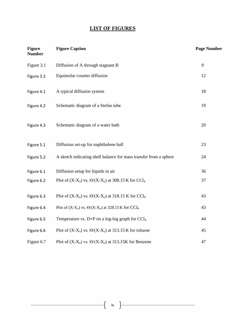
LIST OF FIGURES

Figure

Number

Figure Caption Page Number

Figure 3.1 Diffusion of A through stagnant B 9

Figure 3.2

Equimolar counter diffusion

12

Figure 4.1 A typical diffusion system 18

Figure 4.2 Schematic diagram of a Stefan tube 19

Figure 4.3 Schematic diagram of a water bath

20

Figure 5.1 Diffusion set-up for naphthalene ball 23

Figure 5.2 A sketch indicating shell balance for mass transfer from a sphere 24

Figure 6.1 Diffusion setup for liquids in air 36

Figure 6.2

Plot of (X-Xo) vs. ϴ/(X-Xo) at 308.15 K for CCl4

37

Figure 6.3 Plot of (X-Xo) vs. ϴ/(X-Xo) at 318.15 K for CCl4 43

Figure 6.4 Plot of (X-Xo) vs. ϴ/(X-Xo) at 328.15 K for CCl4

43

Figure 6.5 Temperature vs. D×P on a log-log graph for CCl4 44

Figure 6.6 Plot of (X-Xo) vs. ϴ/(X-Xo) at 313.15 K for toluene 45

Figure 6.7 Plot of (X-Xo) vs. ϴ/(X-Xo) at 313.15K for Benzene

47

x

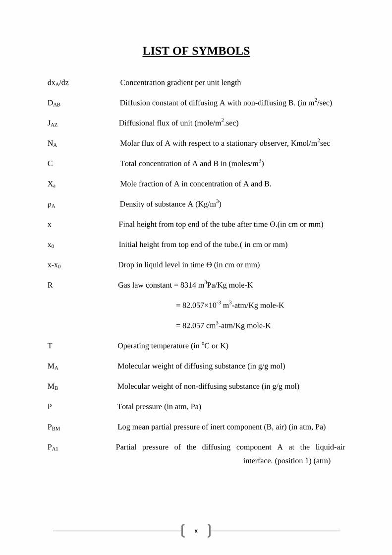
LIST OF SYMBOLS

dxA/dz Concentration gradient per unit length

DAB Diffusion constant of diffusing A with non-diffusing B. (in m2/sec)

JAZ Diffusional flux of unit (mole/m2.sec)

NA Molar flux of A with respect to a stationary observer, Kmol/m2sec

C Total concentration of A and B in (moles/m3)

Xa Mole fraction of A in concentration of A and B.

ρA Density of substance A (Kg/m3)

x Final height from top end of the tube after time ϴ.(in cm or mm)

x0 Initial height from top end of the tube.( in cm or mm)

x-x0 Drop in liquid level in time ϴ (in cm or mm)

R Gas law constant = 8314 m3Pa/Kg mole-K

= 82.057×10-3

m3-atm/Kg mole-K

= 82.057 cm3-atm/Kg mole-K

T Operating temperature (in oC or K)

MA Molecular weight of diffusing substance (in g/g mol)

MB Molecular weight of non-diffusing substance (in g/g mol)

P Total pressure (in atm, Pa)

PBM Log mean partial pressure of inert component (B, air) (in atm, Pa)

PA1 Partial pressure of the diffusing component A at the liquid-air

interface. (position 1) (atm)

xi

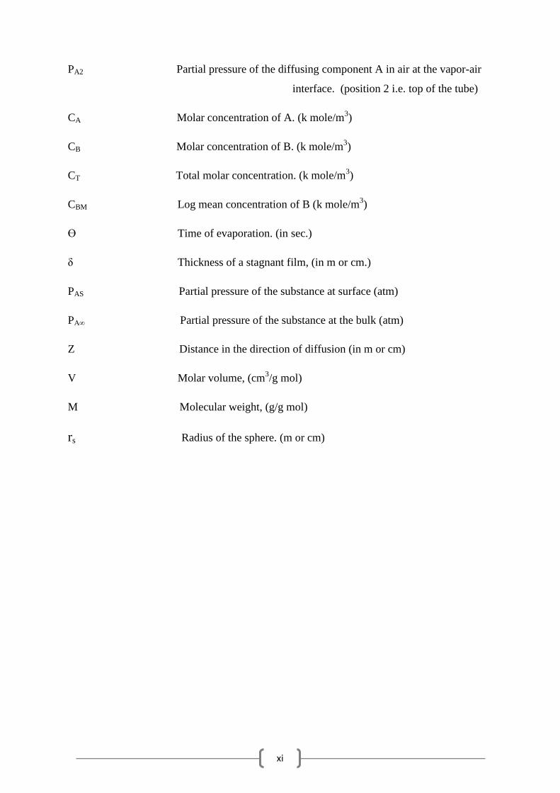
PA2 Partial pressure of the diffusing component A in air at the vapor-air

interface. (position 2 i.e. top of the tube)

CA Molar concentration of A. (k mole/m3)

CB Molar concentration of B. (k mole/m3)

CT Total molar concentration. (k mole/m3)

CBM Log mean concentration of B (k mole/m3)

ϴ Time of evaporation. (in sec.)

δ Thickness of a stagnant film, (in m or cm.)

PAS Partial pressure of the substance at surface (atm)

PA∞ Partial pressure of the substance at the bulk (atm)

Z Distance in the direction of diffusion (in m or cm)

V Molar volume, (cm3/g mol)

M Molecular weight, (g/g mol)

rs Radius of the sphere. (m or cm)

1

CHAPTER 1

INTRODUCTION

1.1 Background of the Research

Mass transfer can either be diffusional or convective. If, there is no external mechanical

disturbance then mass transfer occurs due to diffusion mechanism. However, when there is a

macroscopic disturbance in the medium, which on the other hand greatly influences the rate

of mass transfer, it becomes a convective transport. Thus, the stronger the flow field, creating

more mixing and turbulence in the medium, the higher is rate of mass transfer. The concept

of molecular diffusion is very important and is widely used in variety of scientific and

engineering applications. Whenever there is transport of any gas/liquid/solid molecules occur

through a stagnant zone characterized by a laminar flow regime, the importance of molecular

diffusion is more evident. Even, when there is a turbulent motion sets into the process, there

always remains a laminar zone close to the phase boundary largely influencing the flow

mechanism.

Transport in a porous medium is a classical example where molecular diffusion takes place.

A typical example is the diffusion of reactants and products in a porous catalyst pellet.

Besides normal pore diffusion, Knudsen and surface diffusion as well plays an important role

in determining the performance of a catalyst. To be precise, study of molecular diffusion is

the fundamental basis to the study of mass transfer in general. Mass transfer is the basis of

many chemical and biological processes. Chemical process involve chemical vapour

deposition (CVD) of silane (SiH4) onto a silicon wafer (the doping of silicon wafer lead to the

formation of a silicon thin film), the aeration of waste water leading to its purification, the

purification of ores and isotopes etc. The biological systems include oxygenation of blood

stream and the transport of ions across membrane wihin the kidney etc.

It is important to highlight the fact that any industrial mass transfer operation involves multi-

component system; however, suitable binary system data can be effectively used to estimate

the multi-component system. Similarly, for any unit operation involving more than a single-

phase (and hence presence of an interphase), it is the local or overall mass transfer co-

efficient which explains the mass transfer operation prevailing within the system and can be

effectively. measured in wetted wall column experiments. However, suitably measured

2

diffusivity data can easily be used in estimating the mass transfer coefficients using

fundamental concepts of various predictive theories like (film, penetration, surface renewal

and boundary layer).

1.2 Objective

In this project work, emphasis has been stressed upon to measure the binary diffusion

coefficients of some important organic solvents and solids with varying geometries.

In case of organic solvents acetone, benzene, carbon tetrachloride and toluene are chosen to

be studied. It is a case of diffusion of A (organic solvent) through stagnant non-diffusing B

(air). The experiments are planned to be carried out at widely different temperatures ranging

from 25 to 60oC and at atmospheric pressure, using Stefan tube experiment.

Diffusion coefficients of solids (in air) with varying geometries are also planned to be

studied. Naphthalene balls are selected for studying the diffusion phenomenon in spherical

geometry and Camphor pellets are chosen for studying the diffusion phenomenon in

cylindrical geometry.

1.3 Chapter layout

Chapter 2 is highlighted on the literature review which includes the principle and study of

diffusion and also describes about the laws of diffusion.

Chapter 3 describes about the theories for diffusion of solid materials and liquid solvents

through air and also different data for diffusivities of solids, liquids, and gases also listed.

Chapter 4 is enlighten on the experimental set-ups such as water-bath, stirrer, Stefan tube,

diffusion pump etc.

Chapter 5 is about the experimental diffusion of solids of different geometries such as

spherical naphthalene ball and cylindrical camphor in air and to find out their binary

molecular diffusivities.

Chapter 6 is about the experimental diffusion of different organic liquids (Acetone, CCl4,

Toluene and Benzene) in air and to find out their molecular diffusivities varying with

temperature

Chapter 7 is highlighted on the conclusion and future scopes.

3

CHAPTER 2

LITERATURE REVIEW

2.1 Principles of diffusion

Diffusion is the movement of individual components under the influence of a physical

stimulus through a mixture. The most common cause of diffusion is a concentration gradient

of the diffusing component. A concentration gradient tends to move the component to the

component in such a direction as to equalize concentrations and destroy the gradient. When

the gradient is maintained by constantly supplying the diffusing component to the high-

concentration end of the gradient and removing it at the low-concentration end, there is a

steady-state flux of the diffusing component. This is the characteristic of many mass transfer

operations.

For example, when you spray a perfume in a room, the smell of the perfume spread further

and further and one can smell the perfume in other side. This is nothing but the concept of the

diffusion. The molecules of the perfume when comes in contact with air and forms a

concentration gradient and the components of perfume is tend to move from higher

concentration to the lower concentration and in this way the molecules of the perfume is

being spread and the smell of the perfume can go further and further.

2.2 Theory of diffusion

Molecular diffusion is the thermal motion of liquid or gas particles at temperature above

absolute zero. The rate of this movement is a function of temperature viscosity of the fluid

and the mass or size of the particle. Diffusion explains the net flux of a molecule from a

region of higher concentration to one of lower concentration.

Molecular diffusion or molecular transport can be defined as the transfer or movement of

individual molecules through a fluid by means of the random individual movement of

molecules. Molecular diffusion is typically described mathematically using Fick's laws of

diffusion.

4

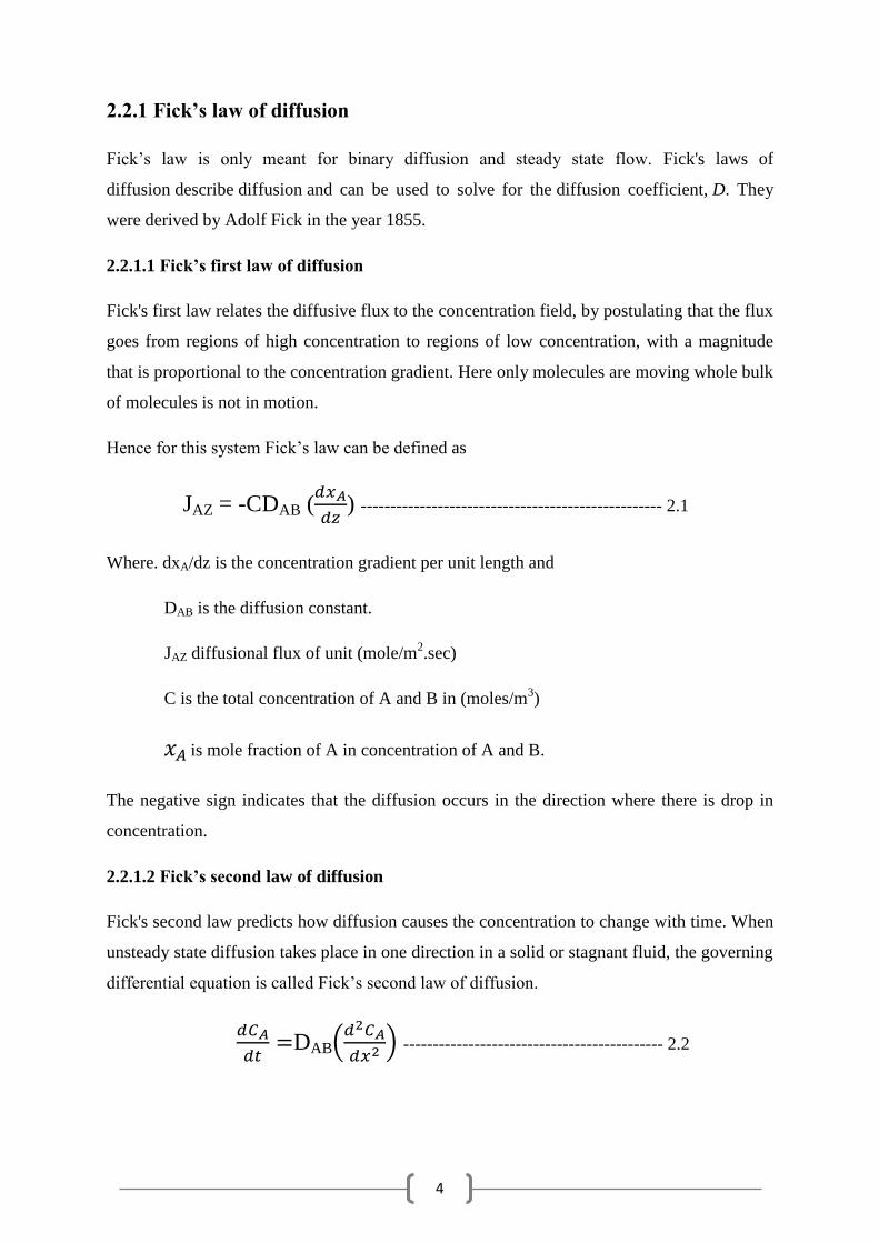
2.2.1 Fick’s law of diffusion

Fick‟s law is only meant for binary diffusion and steady state flow. Fick's laws of

diffusion describe diffusion and can be used to solve for the diffusion coefficient, D. They

were derived by Adolf Fick in the year 1855.

2.2.1.1 Fick’s first law of diffusion

Fick's first law relates the diffusive flux to the concentration field, by postulating that the flux

goes from regions of high concentration to regions of low concentration, with a magnitude

that is proportional to the concentration gradient. Here only molecules are moving whole bulk

of molecules is not in motion.

Hence for this system Fick‟s law can be defined as

JAZ = -CDAB (

) --------------------------------------------------- 2.1

Where. dxA/dz is the concentration gradient per unit length and

DAB is the diffusion constant.

JAZ diffusional flux of unit (mole/m2.sec)

C is the total concentration of A and B in (moles/m3)

is mole fraction of A in concentration of A and B.

The negative sign indicates that the diffusion occurs in the direction where there is drop in

concentration.

2.2.1.2 Fick’s second law of diffusion

Fick's second law predicts how diffusion causes the concentration to change with time. When

unsteady state diffusion takes place in one direction in a solid or stagnant fluid, the governing

differential equation is called Fick‟s second law of diffusion.

DAB(

) -------------------------------------------- 2.2

5

2.3 Types of diffusion

Diffusion is a widespread and important process which occurs in both living and non-living

systems. Because diffusion occurs under a variety of conditions, scientists have adopted

followings to specify particular types of diffusion:

(A) Simple diffusion: it refers to diffusion of substances without the help of transport

proteins.

(B) Facilitated diffusion: it refers to diffusion of substances across a cell membrane with

the help of transport proteins.

(C) Dialysis: It refers to the diffusion of solid across a selectively permeable membrane.

Selectively permeable membrane is a membrane that some substances pass through

easily while other substances pass through very slowly or not at all.

(D) Osmosis: It refers to the diffusion of the solvent across a selectively permeable

membrane. Because water is solvent in all living systems, biologists usually define

osmosis as the diffusion of water across a selectively permeable membrane.

Although various types of diffusion have been recognized, all shares following

characteristics:

(i) Net movement of each substance is caused by random molecular motion.

(ii) Net movement of each substance involves passive transport.

(iii) Net movement of each substance is down its own concentration gradient.

(iv) At equilibrium, random molecular motion continues but there is no longer any net

movement.

6

CHAPTER 3

Diffusion in fluids and Solids

3.1. Steady State Diffusion

In this section, steady-state molecular mass transfer through simple systems in which the

concentration and molar flux are functions of a single space coordinate will be considered. In

a binary system, containing A and B, this molar flux in the direction of z, is given by:

NA= - CDAB

+ YA (NA+NB) ------------------3.1

3.1.1 Diffusion through a stagnant gas film

The diffusivity or diffusion coefficient for a gas can be measured, experimentally using

Arnold diffusion cell. This cell is illustrated schematically in figure. The narrow tube of

uniform cross section which is partially filled with pure liquid A, is maintained at a constant

temperature and pressure. Gas B which flows across the open end of the tub, has a negligible

solubility in liquid A, and is also chemically inert to A. (i.e. no reaction between A & B).

Component A vaporizes and diffuses into the gas phase; the rate of vaporization may be

physically measured and may also be mathematically expressed in terms of the molar flux.

Consider the control volume S Δ z, where S is the cross sectional area of the tube. Mass

balance on „A‟ over this control volume for a steady-state operation yields

[Moles of A leaving at z + Δz] – [Moles of A entering at z] = 0. i.e.,

S NA Z+ΔZ – S NA Z = 0 ------------------------------- 3.2

Dividing through by the volume, SΔZ, and evaluating in the limit as ΔZ approaches zero, we

obtain the differential equation;

This relation stipulates a constant molar flux of A throughout the gas phase from Z1 to Z2. A

similar differential equation could also be written for component B as;

7

And accordingly, the molar flux of B is also constant over the entire diffusion path from z1

and z2.

Considering only at plane z1, and since the gas B is insoluble is liquid A, we realize that NB,

the net flux of B, is zero throughout the diffusion path; accordingly B is a stagnant gas.

From equation (3.1)

NA= - CDAB

+ YA (NA+NB)

Since NB=0

NA= - CDAB

+ YANA

By rearranging

NA= -CDAB (

)

--------------------------------------3.3

This equation may be integrated between the two boundary conditions:

At z = z1 YA = YA1 and at z = z2 YA = YA2

Assuming the diffusivity is to be independent of concentration, and realizing that NA is

constant along the diffusion path, by integrating equation (ii) we obtain

∫

∫

(

) --------------------------- 3.4

8

The log mean average concentration of component B is defined as

.

/

Since, YB=1-YA

( ) ( )

(

)

(

) ------------------------- 3.5

Substituting from Equation (3.5) in Equation (3.4),

( )

-------------------------------------- 3.6

For an ideal gas

and

For mixture of ideal gases

Therefore, for an ideal gas mixture equation. (3.6) Becomes

( )

( )

-------------------------------- 3.7

This is the equation of molar flux for steady state diffusion of one gas through a second

stagnant gas.

Where

DAB = molecular diffusivity of A in B

R = universal gas constant

T = temperature of system in absolute scale

z = distance between two planes across the direction of diffusion

PA1 = partial pressure of A at plane 1, and

PA2 = partial pressure of A at plane 2

9

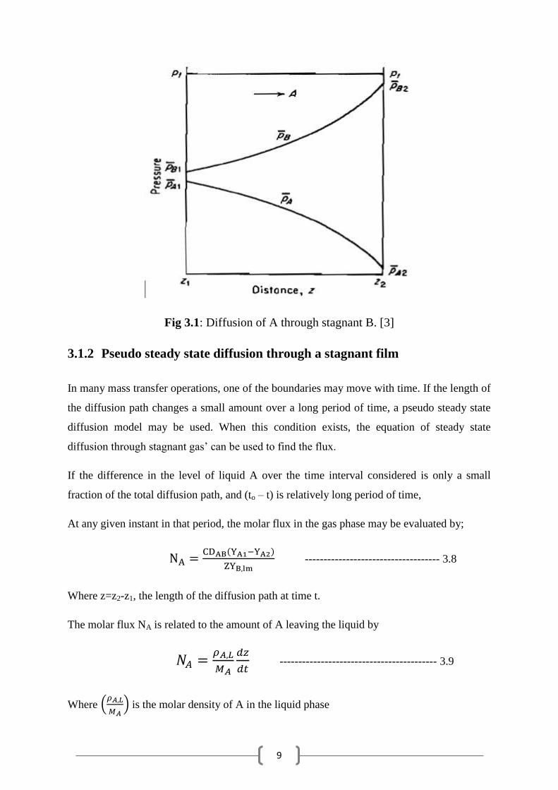
Fig 3.1: Diffusion of A through stagnant B. [3]

3.1.2 Pseudo steady state diffusion through a stagnant film

In many mass transfer operations, one of the boundaries may move with time. If the length of

the diffusion path changes a small amount over a long period of time, a pseudo steady state

diffusion model may be used. When this condition exists, the equation of steady state

diffusion through stagnant gas‟ can be used to find the flux.

If the difference in the level of liquid A over the time interval considered is only a small

fraction of the total diffusion path, and (to – t) is relatively long period of time,

At any given instant in that period, the molar flux in the gas phase may be evaluated by;

( )

------------------------------------ 3.8

Where z=z2-z1, the length of the diffusion path at time t.

The molar flux NA is related to the amount of A leaving the liquid by

------------------------------------------ 3.9

Where (

) is the molar density of A in the liquid phase

10

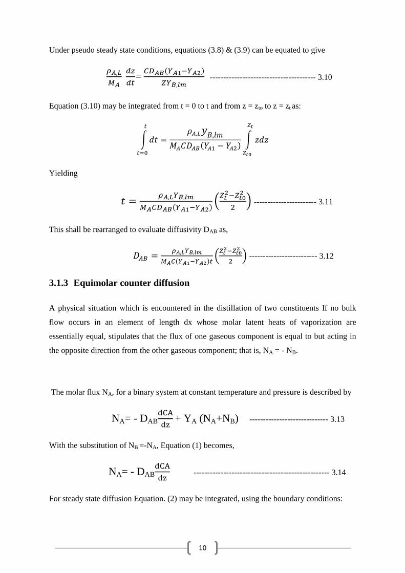
Under pseudo steady state conditions, equations (3.8) & (3.9) can be equated to give

= ( )

--------------------------------------- 3.10

Equation (3.10) may be integrated from t = 0 to t and from z = zto to z = zt as:

∫

( )∫

Yielding

( )(

) ----------------------- 3.11

This shall be rearranged to evaluate diffusivity DAB as,

( ) (

) ------------------------- 3.12

3.1.3 Equimolar counter diffusion

A physical situation which is encountered in the distillation of two constituents If no bulk

flow occurs in an element of length dx whose molar latent heats of vaporization are

essentially equal, stipulates that the flux of one gaseous component is equal to but acting in

the opposite direction from the other gaseous component; that is, NA = - NB.

The molar flux NA, for a binary system at constant temperature and pressure is described by

NA= - DAB

+ YA (NA+NB) ----------------------------- 3.13

With the substitution of NB =-NA, Equation (1) becomes,

NA= - DAB

-------------------------------------------------- 3.14

For steady state diffusion Equation. (2) may be integrated, using the boundary conditions:

11

At z = z1: CA = CA1 and z = z2: CA = CA2

Giving,

∫

∫

From which

NA= -

( ) ------------------------------- 3.15

For ideal gases,

.

Therefore equation (3.14) becomes:

NA= -

( )( ) ------------------------------- 3.16

This is the equation of molar flux for steady-state equimolar counter diffusion.

Concentration profile in this equimolar counter diffusion may be obtained from,

( ) (Since NA is constant over the diffusion path)

And from equation (3.14)

NA= - DAB

Therefore

(

)

This equation may be solved using the boundary conditions to give

--------------------------------------------- 3.17

Equation (3.17) indicates a linear concentration profile for equimolar counter diffusion.

12

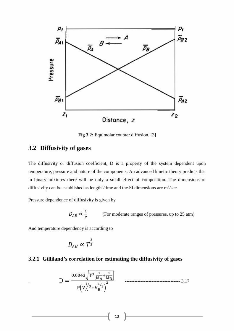
Fig 3.2: Equimolar counter diffusion. [3]

3.2 Diffusivity of gases

The diffusivity or diffusion coefficient, D is a property of the system dependent upon

temperature, pressure and nature of the components. An advanced kinetic theory predicts that

in binary mixtures there will be only a small effect of composition. The dimensions of

diffusivity can be established as length2/time and the SI dimensions are m

2/sec.

Pressure dependence of diffusivity is given by

(For moderate ranges of pressures, up to 25 atm)

And temperature dependency is according to

3.2.1 Gilliland’s correlation for estimating the diffusivity of gases

. √ [

]

(

⁄

⁄ ) ----------------------------------- 3.17

13

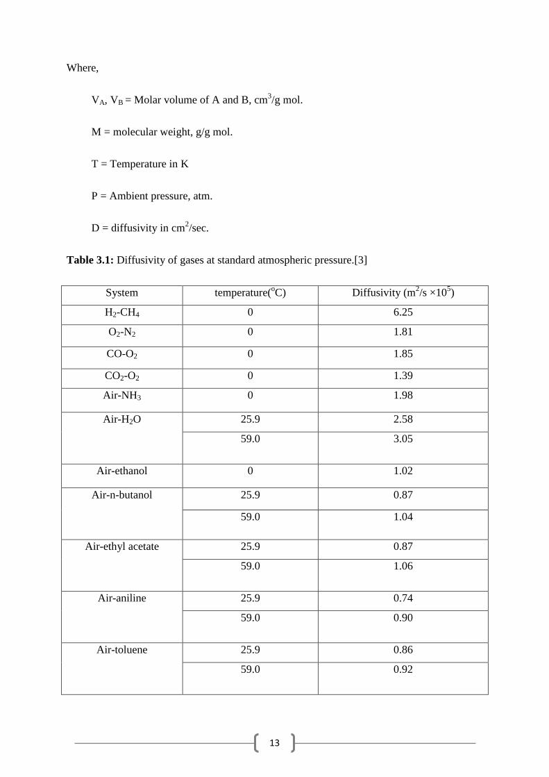
Where,

VA, VB = Molar volume of A and B, cm3/g mol.

M = molecular weight, g/g mol.

T = Temperature in K

P = Ambient pressure, atm.

D = diffusivity in cm2/sec.

Table 3.1: Diffusivity of gases at standard atmospheric pressure.[3]

System temperature(oC) Diffusivity (m

2/s ×10

5)

H2-CH4 0 6.25

O2-N2 0 1.81

CO-O2 0 1.85

CO2-O2 0 1.39

Air-NH3 0 1.98

Air-H2O

25.9 2.58

59.0 3.05

Air-ethanol 0 1.02

Air-n-butanol

25.9 0.87

59.0 1.04

Air-ethyl acetate

25.9 0.87

59.0 1.06

Air-aniline

25.9 0.74

59.0 0.90

Air-toluene

25.9 0.86

59.0 0.92

14

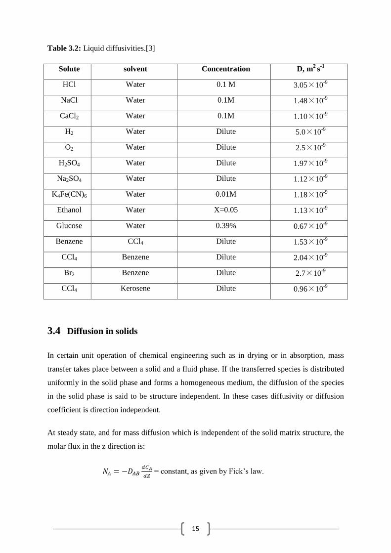
3.3 Diffusivity in liquids

Diffusivity in liquid are exemplified by the values, most of these are nearer to 10-5

cm2/sec,

and about ten thousand times shower than those in dilute gases. This characteristic of liquid

diffusion often limits the overall rate of processes accruing in liquids such as reaction

between two components in liquids. In chemistry, diffusivity limits the rate of acid-base

reactions; in the chemical industry, diffusion is responsible for the rates of liquid-liquid

extraction.

Diffusion in liquids is important because it is slow. Certain molecules diffuse as molecules,

while others which are designated as electrolytes ionize in solutions and diffuse as ions. For

example, sodium chloride (NaCl), diffuses in water as ions Na+ and Cl

-. Though each ions

has a different mobility, the electrical neutrality of the solution indicates the ions must diffuse

at the same rate; accordingly it is possible to speak of a diffusion coefficient for molecular

electrolytes such as NaCl. However, if several ions are present, the diffusion rates of the

individual cations and anions must be considered, and molecular diffusion coefficients have

no meaning. Diffusivity varies inversely with viscosity when the ratio of solute to solvent

ratio exceeds five. In extremely high viscosity materials, diffusion becomes independent of

viscosity.

15

Table 3.2: Liquid diffusivities.[3]

Solute

solvent

Concentration

D, m2

s-1

HCl Water 0.1 M 3.05×10-9

NaCl Water 0.1M 1.48×10-9

CaCl2 Water 0.1M 1.10×10-9

H2 Water Dilute 5.0×10-9

O2 Water Dilute 2.5×10-9

H2SO4 Water Dilute 1.97×10-9

Na2SO4 Water Dilute 1.12×10-9

K4Fe(CN)6 Water 0.01M 1.18×10-9

Ethanol Water X=0.05 1.13×10-9

Glucose Water 0.39% 0.67×10-9

Benzene CCl4 Dilute 1.53×10-9

CCl4 Benzene Dilute 2.04×10-9

Br2 Benzene Dilute 2.7×10-9

CCl4 Kerosene Dilute 0.96×10-9

3.4 Diffusion in solids

In certain unit operation of chemical engineering such as in drying or in absorption, mass

transfer takes place between a solid and a fluid phase. If the transferred species is distributed

uniformly in the solid phase and forms a homogeneous medium, the diffusion of the species

in the solid phase is said to be structure independent. In these cases diffusivity or diffusion

coefficient is direction independent.

At steady state, and for mass diffusion which is independent of the solid matrix structure, the

molar flux in the z direction is:

= constant, as given by Fick‟s law.

16

( )

Which is similar to the expression obtained for diffusion in a stagnant fluid with no bulk

motion (i.e. N = 0).

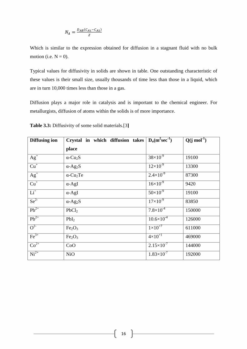
Typical values for diffusivity in solids are shown in table. One outstanding characteristic of

these values is their small size, usually thousands of time less than those in a liquid, which

are in turn 10,000 times less than those in a gas.

Diffusion plays a major role in catalysis and is important to the chemical engineer. For

metallurgists, diffusion of atoms within the solids is of more importance.

Table 3.3: Diffusivity of some solid materials.[3]

Diffusing ion Crystal in which diffusion takes

place

Do(m2sec

-1) Q(j mol

-1)

Ag+ α-Cu2S 38×10

-9 19100

Cu+ α-Ag2S 12×10

-9 13300

Ag+ α-Cu2Te 2.4×10

-9 87300

Cu+ α-AgI 16×10

-9 9420

Li+ α-AgI 50×10

-9 19100

Se2-

α-Ag2S 17×10-9

83850

Pb2+

PbCl2 7.8×10-4

150000

Pb2+

PbI2 10.6×10-4

126000

O2-

Fe2O3 1×10+7

611000

Fe3+

Fe2O3 4×10+1

469000

Co2+

CoO 2.15×10-7

144000

Ni2+

NiO 1.83×10-7

192000

17

CHAPTER 4

Diffusion setups

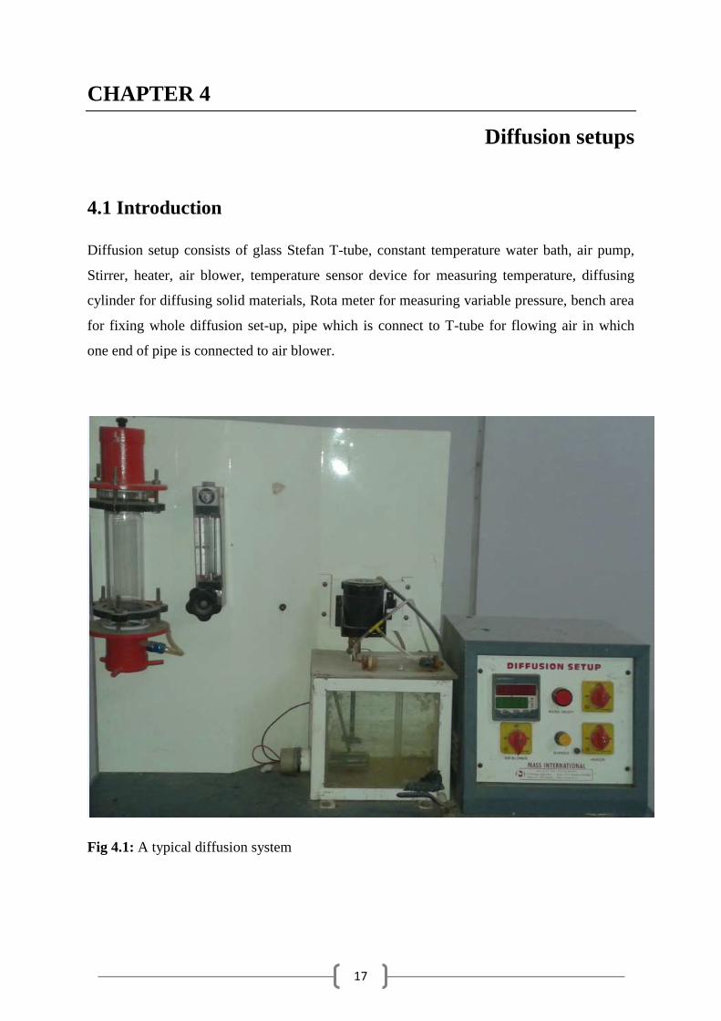
4.1 Introduction

Diffusion setup consists of glass Stefan T-tube, constant temperature water bath, air pump,

Stirrer, heater, air blower, temperature sensor device for measuring temperature, diffusing

cylinder for diffusing solid materials, Rota meter for measuring variable pressure, bench area

for fixing whole diffusion set-up, pipe which is connect to T-tube for flowing air in which

one end of pipe is connected to air blower.

Fig 4.1: A typical diffusion system

18

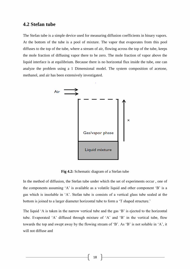
4.2 Stefan tube

The Stefan tube is a simple device used for measuring diffusion coefficients in binary vapors.

At the bottom of the tube is a pool of mixture. The vapor that evaporates from this pool

diffuses to the top of the tube, where a stream of air, flowing across the top of the tube, keeps

the mole fraction of diffusing vapor there to be zero. The mole fraction of vapor above the

liquid interface is at equilibrium. Because there is no horizontal flux inside the tube, one can

analyze the problem using a 1 Dimensional model. The system composition of acetone,

methanol, and air has been extensively investigated.

Fig 4.2: Schematic diagram of a Stefan tube

In the method of diffusion, the Stefan tube under which the set of experiments occur , one of

the components assuming „A‟ is available as a volatile liquid and other component „B‟ is a

gas which is insoluble in „A‟. Stefan tube is consists of a vertical glass tube sealed at the

bottom is joined to a larger diameter horizontal tube to form a „T shaped structure.‟

The liquid „A is taken in the narrow vertical tube and the gas „B‟ is ejected to the horizontal

tube. Evaporated „A‟ diffused through mixture of „A‟ and „B‟ in the vertical tube, flow

towards the top and swept away by the flowing stream of „B‟. As „B‟ is not soluble in „A‟, it

will not diffuse and

19

the statement is confirmed to be “Diffusion of „A‟ through non-diffusing „B‟. The liquid tube

level will gradually drop slowly and pseudo-steady state assumption is reached.

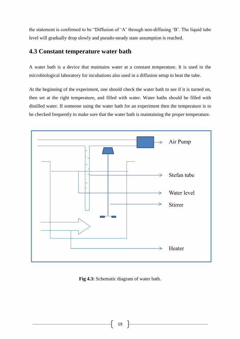
4.3 Constant temperature water bath

A water bath is a device that maintains water at a constant temperature. It is used in the

microbiological laboratory for incubations also used in a diffusion setup to heat the tube.

At the beginning of the experiment, one should check the water bath to see if it is turned on,

then set at the right temperature, and filled with water. Water baths should be filled with

distilled water. If someone using the water bath for an experiment then the temperature is to

be checked frequently to make sure that the water bath is maintaining the proper temperature.

Fig 4.3: Schematic diagram of water bath.

Air Pump

Stefan tube

Stirrer

Heater

Water level

Fig 4.3: Schematic diagram of a water Bath

20

4.3.1 Temperature Control

All water baths have a control to set temperature. This control can be digital or a dial. Often

there is an indicator light associated with this control. When the light is on the water bath is

heating. When the water bath reaches the set temperature, it will cycle on and off to maintain

constant temperature.

4.3.2 Safety Control

Most water baths have a second control called the safety. This control is set at the maximum

temperature the water bath should attain. It is usually set just above the temperature control.

Often an indicator light is associated with the safety control. If the water bath reaches the

temperature that the safety control is set at, the light will go on. It will be impossible for the

water bath to heat higher than the safety setting even when the temperature setting is higher.

If your water bath stays a temperature lower than the temperature control setting, try

increasing the safety control setting.

4.4 Stirrer

A stirrer is a laboratory device that employs a rotating rod to cause a stir bar submerged in a

liquid to spin very quickly. The rotating field may be created either by a motor or a set of

stationary electromagnets, placed in the vessel with the liquid. Since glass does not affect

a magnetic field affectively , and most chemical reactions take place in glass vessels such

as beaker (glassware) or laboratory flasks, magnetic stir bars work well in glass vessels. They

also have difficulty dealing with viscous liquids or thick suspensions. For larger volumes or

more viscous liquids, some sort of mechanical stirring is typically needed.

The stirrers are distinguished according to the type of flow they generate in the stirred

material, the speed-depending applications and the various designs for different viscosities.

Stirrers are often used in chemistry and biology. They are preferred over gear-

driven motorized stirrers because they are quieter, more efficient, and have no moving

external parts to break or wear out. Because of its small size, a stirring bar is more easily

cleaned and sterilized than other stirring devices. They do not require lubricants which could

contaminate the reaction vessel and the product. They can be used inside tightly closed

vessels or systems, without the need for complicated rotary seals.

21

4.4 Diffusion pumps

Diffusion pumps use a high speed jet of vapor to direct gas molecules in the pump throat

down into the bottom of the pump and out the exhaust. Invented in 1915 by Wolfgang Gaede

using mercury vapor, and improved by Irving Langmuir and W. Crawford, they were the first

type of high vacuum pumps operating in the regime of free molecular flow, where the

movement of the gas molecules can be better understood as diffusion than by

conventional fluid dynamics. Gaede used the name diffusion pump since his design was

based on the finding that gas cannot diffuse against the vapor stream, but will be carried with

it to the exhaust. However, the principle of operation might be more precisely described

as gas-jet pump, since diffusion plays a role also in other high vacuum pumps. An air pump is

a device for pushing air.

22

CHAPTER 5

Solids of different geometries diffused in Air

5.1 Objective

To study the diffusion of spherical naphthalene ball and cylindrical camphor in air and to

determine their diffusivities.

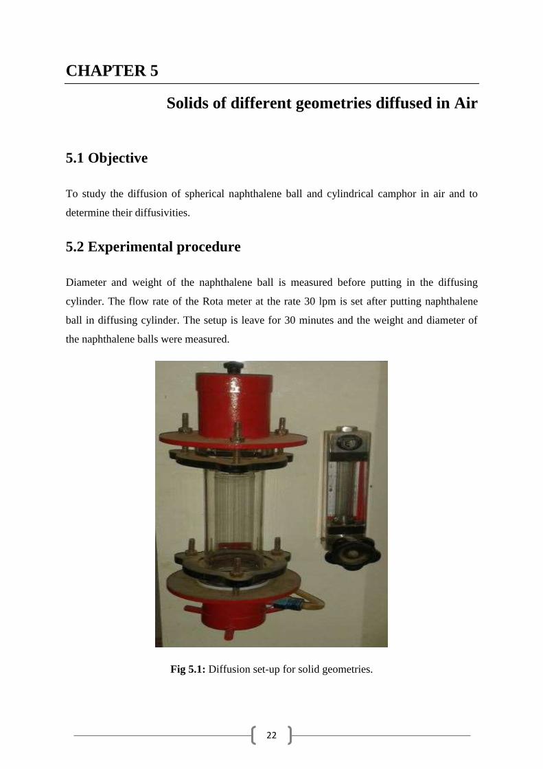
5.2 Experimental procedure

Diameter and weight of the naphthalene ball is measured before putting in the diffusing

cylinder. The flow rate of the Rota meter at the rate 30 lpm is set after putting naphthalene

ball in diffusing cylinder. The setup is leave for 30 minutes and the weight and diameter of

the naphthalene balls were measured.

Fig 5.1: Diffusion set-up for solid geometries.

23

5.3 Theory

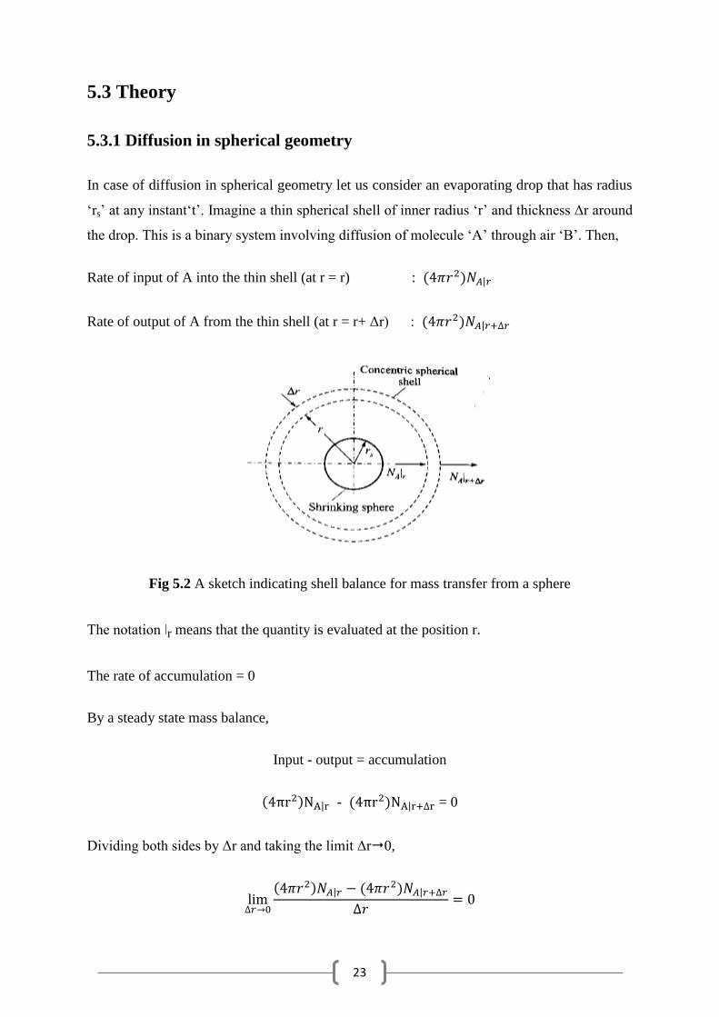
5.3.1 Diffusion in spherical geometry

In case of diffusion in spherical geometry let us consider an evaporating drop that has radius

„rs‟ at any instant„t‟. Imagine a thin spherical shell of inner radius „r‟ and thickness Δr around

the drop. This is a binary system involving diffusion of molecule „A‟ through air „B‟. Then,

Rate of input of A into the thin shell (at r = r) : ( ) |

Rate of output of A from the thin shell (at r = r+ Δr) : ( ) |

Fig 5.2 A sketch indicating shell balance for mass transfer from a sphere

The notation ǀr means that the quantity is evaluated at the position r.

The rate of accumulation = 0

By a steady state mass balance,

Input - output = accumulation

( ) | - ( ) | = 0

Dividing both sides by Δr and taking the limit Δr0,

( ) | ( ) |

24

( )

= constant = W (say) ----------------------------------- 5.1

Equation 5.1 is a very important result for steady state diffusion through a variable area and

can be generalized as

(Area)(Flux) = Constant ------------------------------------------- 5.2

In this case molecule A diffuses, but air does not diffuse because it is not soluble in the

molecule. So, the case corresponds to diffusion of A through non diffusing B. Since diffusion

occurs in radial condition, we get

( )

Putting NB = 0 and rearranging,

( )

------------------------------------- 5.3

From equation 5.1 and 5.3,

----------------------------------------- 5.4

Equation 5.4 can be integrated from r = rs (i.e. the surface of the molecule) to r = ∞ (i.e. far

away from the drop) where PA=PA∞

Here PAS is the vapour pressure of the molecule at the temperature of the surface and PA∞ is

the partial pressure of the molecule in the bulk air.

∫

=

∫

------------------------------5.5

25

Since W is the constant molar rate of mass transfer, it is equal to the rate of vaporization of

the molecule at any instant.

This rate can be related to the change in the molecule radius by the following equation.

(

)

------------------------------5.6

The negative sign is incorporated because the size of the molecule decreases with time.

Equating equations 5.5 and 5.6,

Here gain we have made use of the „pseudo-steady state‟ assumption, that the molecule size

changes so slowly that the diffusion of the substance through the surrounding air occurs

virtually at steady state all time. The change in the molecule size over considerable period of

time can be determined by integrating the above equation.

If at time t = 0, the radius of the molecule is rs0 and at time t it is rs. Then,

∫

∫

-------------------------5.7

Hence diffusivity of the molecule in the spherical geometry is calculated as

(

)

(

) ---------------------------------------5.8

5.3.2 Diffusion in cylindrical geometry

This is the case of diffusion of A (cylindrical substance) through non-diffusing B (air)

through a variable area. Taking the help of equation 5.2 and 5.3, we may write

( ) ( ) (

( ))

(Constant) ----------- 5.9

26

L= length of the cylinder

Here r is the radial distance of any point within surrounding air film from the axis of the

cylinder.

W is the molar rate of sublimation

Distance r varies from radius of the cylinder (rc) to the outer edge of the air-film (rc+δ) where

δ is the thickness of the film.

The corresponding values of the partial pressure of cylindrical substance are,

At r = rc, PA = PAs (sublimation pressure)

At r = rc+δ, PA = 0, as there is no molecules of the substance in bulk air.

To calculate the rate of sublimation, we have to integrate the equation 5.9.

∫

=

∫

(

)

(

)

----------------------------------------5.10

In order to calculate the required time of sublimation, we make the usual pseudo-steady state

approximation.

If at any time t the mass of the cylinder,

Then the rate of sublimation neglecting the end losses can be expressed as

( ⁄ )

(

) (

)

------------------ 5.11

MA is the molecular weight.

27

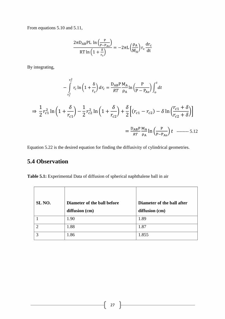
From equations 5.10 and 5.11,

(

)

(

)

( )

By integrating,

∫ (

)

(

)∫

(

)

(

)

[( ) (

)]

(

) -------- 5.12

Equation 5.22 is the desired equation for finding the diffusivity of cylindrical geometries.

5.4 Observation

Table 5.1: Experimental Data of diffusion of spherical naphthalene ball in air

SL NO.

Diameter of the ball before

diffusion (cm)

Diameter of the ball after

diffusion (cm)

1 1.90 1.89

2 1.88 1.87

3 1.86 1.855

28

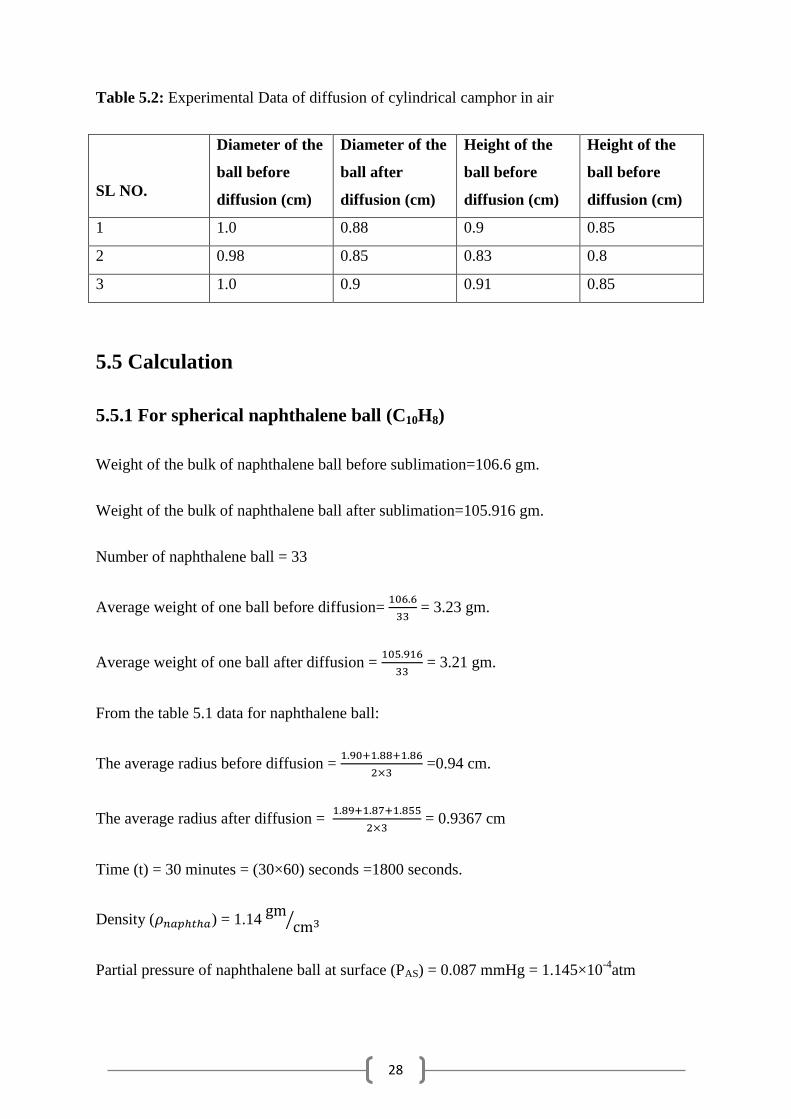
Table 5.2: Experimental Data of diffusion of cylindrical camphor in air

SL NO.

Diameter of the

ball before

diffusion (cm)

Diameter of the

ball after

diffusion (cm)

Height of the

ball before

diffusion (cm)

Height of the

ball before

diffusion (cm)

1 1.0 0.88 0.9 0.85

2 0.98 0.85 0.83 0.8

3 1.0 0.9 0.91 0.85

5.5 Calculation

5.5.1 For spherical naphthalene ball (C10H8)

Weight of the bulk of naphthalene ball before sublimation=106.6 gm.

Weight of the bulk of naphthalene ball after sublimation=105.916 gm.

Number of naphthalene ball = 33

Average weight of one ball before diffusion=

= 3.23 gm.

Average weight of one ball after diffusion =

= 3.21 gm.

From the table 5.1 data for naphthalene ball:

The average radius before diffusion =

=0.94 cm.

The average radius after diffusion =

= 0.9367 cm

Time (t) = 30 minutes = (30×60) seconds =1800 seconds.

Density ( ) = 1.14

⁄

Partial pressure of naphthalene ball at surface (PAS) = 0.087 mmHg = 1.145×10-4

atm

29

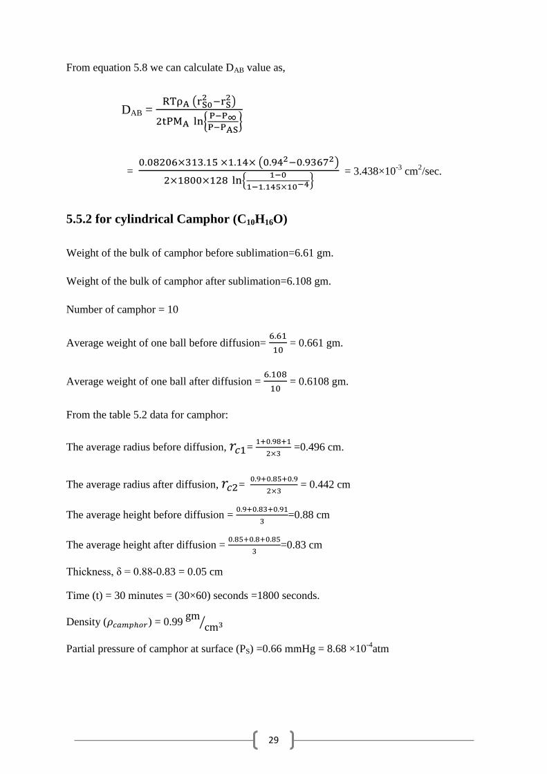
From equation 5.8 we can calculate DAB value as,

DAB = (

)

{

}

= ( )

,

-

= 3.438×10-3

cm2/sec.

5.5.2 for cylindrical Camphor (C10H16O)

Weight of the bulk of camphor before sublimation=6.61 gm.

Weight of the bulk of camphor after sublimation=6.108 gm.

Number of camphor = 10

Average weight of one ball before diffusion=

= 0.661 gm.

Average weight of one ball after diffusion =

= 0.6108 gm.

From the table 5.2 data for camphor:

The average radius before diffusion, =

=0.496 cm.

The average radius after diffusion, =

= 0.442 cm

The average height before diffusion =

=0.88 cm

The average height after diffusion =

=0.83 cm

Thickness, δ = 0.88-0.83 = 0.05 cm

Time (t) = 30 minutes = (30×60) seconds =1800 seconds.

Density ( ) = 0.99

⁄

Partial pressure of camphor at surface (PS) =0.66 mmHg = 8.68 ×10-4

atm

30

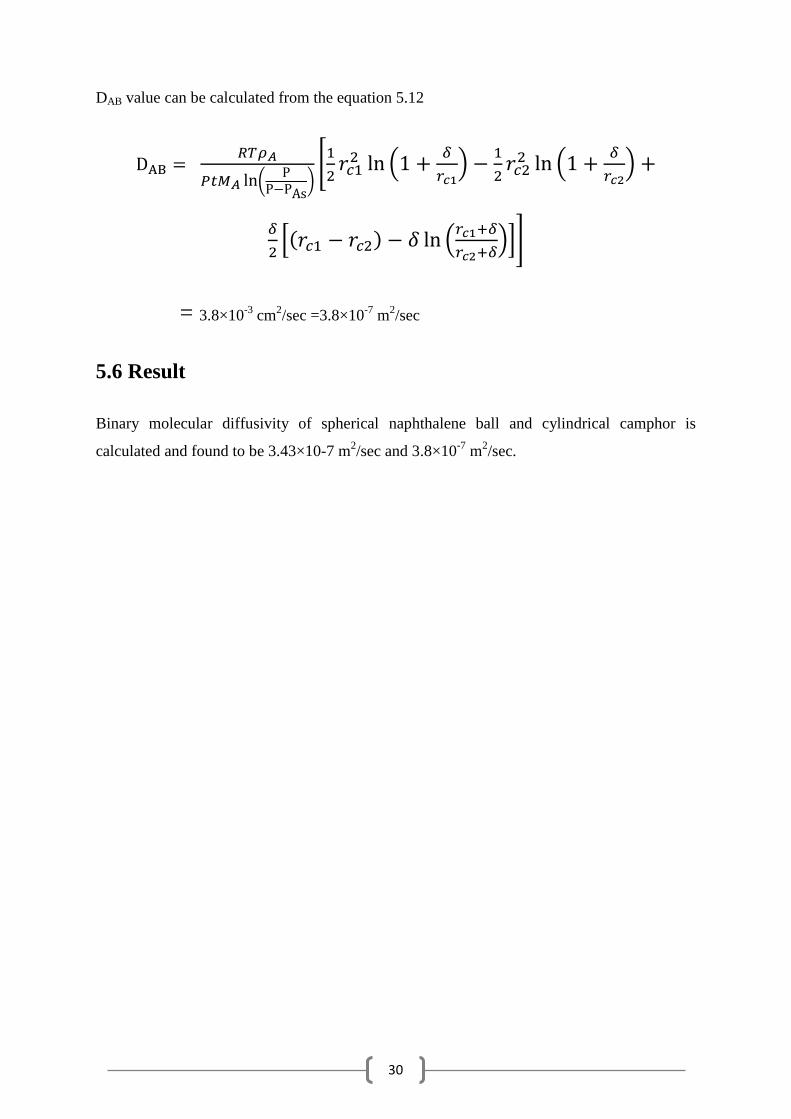
DAB value can be calculated from the equation 5.12

(

)0

(

)

(

)

*( ) (

)+1

= 3.8×10-3

cm2/sec =3.8×10

-7 m

2/sec

5.6 Result

Binary molecular diffusivity of spherical naphthalene ball and cylindrical camphor is

calculated and found to be 3.43×10-7 m2/sec and 3.8×10

-7 m

2/sec.

31

CHAPTER 6

Organic liquids diffused in air

6.1 Objective

Determination of the diffusion co-efficient of an organic vapor in air.

To study the effect of temperature on the diffusion co-efficient.

6.2 Theory

If two gases are inter-diffusing with continual supply of fresh gas and removal of the

products of diffusion, this diffusion reaches an equilibrium state with constant concentration

gradients. This is known as steady state diffusion. If also there is no total flow in either

direction of rates of diffusion of A and B. NA and NB are equal but have opposite sign.

According to Dalton‟s law the total concentration of the two components CA and CB is

constant.

=

------------------------------------------------------- 6.1

Then using the integrated form of the Fick Diffusion equation with appropriate constants:

------------------------------------------------ 6.2

------------------------------------------------- 6.3

Where DAB = DBA =Diffusivity coefficient of A/B.

Molar concentration of a perfect gas CA is related to partial pressure PA by the gas law:

Then,

----------------------------------------------------------- 6.4

Integration of equation-7.4 yields,

( )

( ) --------------------------------- 6.5

Where PA1 and PA2 are the partial pressures of A at the boundaries of the zone of diffusion

and x is the distance over which diffusion occurs.

32

In case where gas A is diffusing through stagnant gas non-diffusing B, the flow carries both

components in proportions to their partial pressure

.

The total transfer of A is the sum of this proportion of the flow and the transfer by diffusion.

------------------------------------------------- 6.6

Or

(

)

--------------------------------------------- 6.7

Or

∫

∫

----------------------------------------------------- 6.8

And

------------------------------------------------------------ 6.9

Equation 7.9 is the expression used for the determination of vapour diffusion coefficients in

gases by evaporation from a surface of liquid in a thinner bore tube and measuring the level

of the falling liquid surface.

The distance of the liquid surface below the open end of the tube is measured before and after

evaporation over a particular period of time. If the change in level is small then the arithmetic

mean of these two readings is taken as the value of x.

In case there is some change of level, the value of x is determined by integration between the

initial and final readings of level.

Thus, the rate of evaporation is given by,

------------------------------------------------ 6.10

Where

M= molecular weight of evaporating liquid

ρ1=density of evaporating liquid

Integration of this expression yields:

33

(

)

∫

∫

--------------------------------------------- 6.11

(

)

--------------------------------------------------- 6.12

Therefore,

(

)

---------------------------------------------------- 6.13

ϴ is the time of evaporation.

Other form of equation which is convenient to use is:

(

)

( ) ----------------------------------------------------- 6.14

In terms of concentration terms the expression for D is:

--------------------------------------------------- 6.15

(

) ----------------------------------------------------------------- 6.16

Usually, xo will not be measured accurately nor is the effective distance for diffusion, x at

time ϴ. Accurate value of (x-xo) is available.

Rewriting eq-7.15 as,

( )

------------------ 6.17

A graph between

against (x-xo) should yield a straight line with slope

----------------------------------------------------------- 6.18

------------------------------------------------------- 6.19

34

If we take kilogram molecular volume of a gas as 22.4 m3, then

-------------------------------------------------------------- 6.20

If the vapour pressure of evaporating liquid A is vapour pressure (KN/m2) at the operating

temperature of 0K. Then,

( )

( ) -------------------------------------- 6.21

Effect of temperature and pressure on co-efficient of diffusion, D is expressed as:

D= Const. T1.5

/P -------------------------------------------------------- 6.22

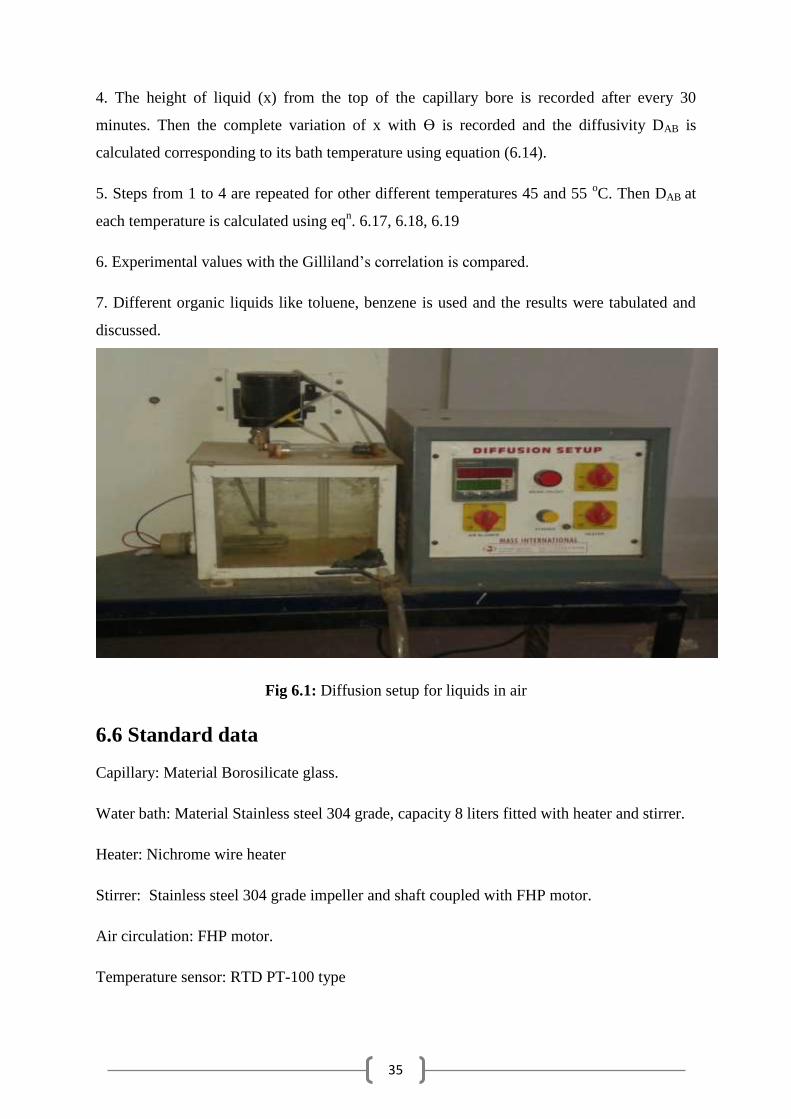
6.3 Description

The main components of the experimental set-up are:

Glass T-tube, constant temperature water bath, Air pump, Scale for measurement,

Volatile component is filled in the T-tube and air is passed over it by the pump and changes

in the level are measured by the measuring centimeter scale.

6.4 Utilities Required

Electricity supply: 1 phase, 220 V AC and 0.6 KW

Required chemicals such as Acetone, CCl4, toluene, and benzene and laboratory glassware.

Bench area 1.2 m × 0.75 m

6.5 Experimental Procedure

1. The water bath temperature is set at the desired level between 25 oC to 60

oC and to wait till

the bath attains the set temperature. Steady temperature of the bath is noted down.

2. The T-tube is filled with CCl4 to within 2 centimeters of the top of capillary leg. The initial

diffusion height of the liquid in the capillary from the top is noted down (xo).

3. Then the connection with the air of vacuum pump is made and a gentle current of air is

allowed to flow over the capillary.

35

4. The height of liquid (x) from the top of the capillary bore is recorded after every 30

minutes. Then the complete variation of x with ϴ is recorded and the diffusivity DAB is

calculated corresponding to its bath temperature using equation (6.14).

5. Steps from 1 to 4 are repeated for other different temperatures 45 and 55 oC. Then DAB at

each temperature is calculated using eqn. 6.17, 6.18, 6.19

6. Experimental values with the Gilliland‟s correlation is compared.

7. Different organic liquids like toluene, benzene is used and the results were tabulated and

discussed.

Fig 6.1: Diffusion setup for liquids in air

6.6 Standard data

Capillary: Material Borosilicate glass.

Water bath: Material Stainless steel 304 grade, capacity 8 liters fitted with heater and stirrer.

Heater: Nichrome wire heater

Stirrer: Stainless steel 304 grade impeller and shaft coupled with FHP motor.

Air circulation: FHP motor.

Temperature sensor: RTD PT-100 type

36

Control panel comprising of:

Digital temperature controller cum-indicator, standard make on-off switch, mains indicator

etc.

The whole set-up is fixed on a powder coated base plate.

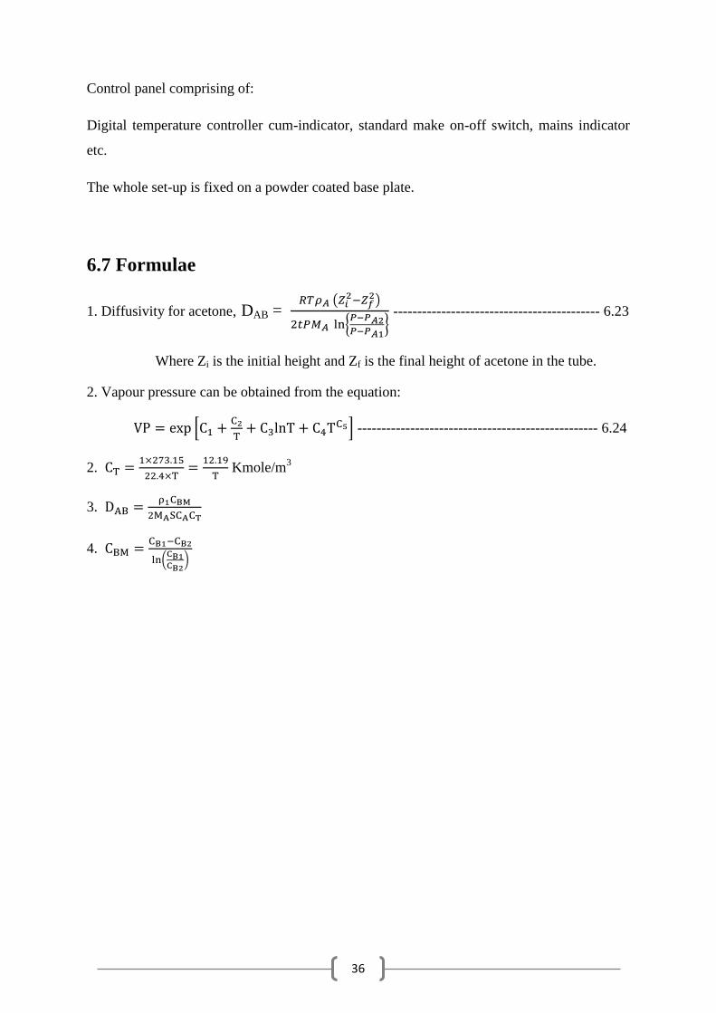
6.7 Formulae

1. Diffusivity for acetone, DAB = (

)

{

} ------------------------------------------- 6.23

Where Zi is the initial height and Zf is the final height of acetone in the tube.

2. Vapour pressure can be obtained from the equation:

*

+ -------------------------------------------------- 6.24

2.

Kmole/m

3

3.

4.

(

)

37

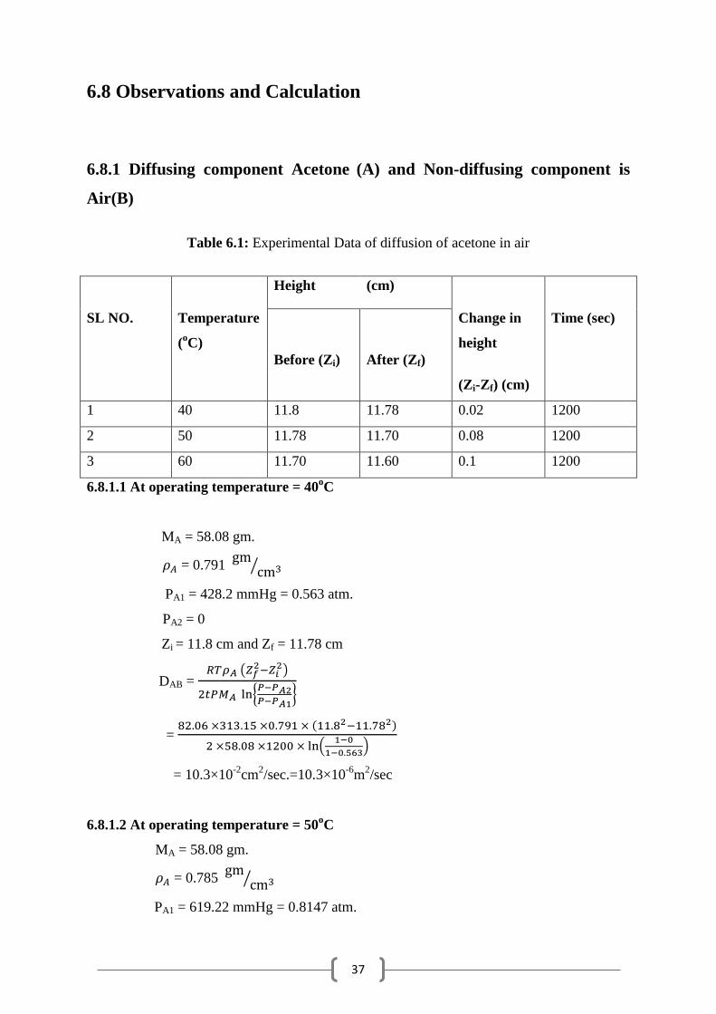
6.8 Observations and Calculation

6.8.1 Diffusing component Acetone (A) and Non-diffusing component is

Air(B)

Table 6.1: Experimental Data of diffusion of acetone in air

Height (cm)

SL NO. Temperature

(oC)

Before (Zi)

After (Zf)

Change in

height

(Zi-Zf) (cm)

Time (sec)

1 40 11.8 11.78 0.02 1200

2 50 11.78 11.70 0.08 1200

3 60 11.70 11.60 0.1 1200

6.8.1.1 At operating temperature = 40oC

MA = 58.08 gm.

= 0.791

⁄

PA1 = 428.2 mmHg = 0.563 atm.

PA2 = 0

Zi = 11.8 cm and Zf = 11.78 cm

DAB = (

)

{

}

= ( )

(

)

= 10.3×10-2

cm2/sec.=10.3×10

-6m

2/sec

6.8.1.2 At operating temperature = 50oC

MA = 58.08 gm.

= 0.785

⁄

PA1 = 619.22 mmHg = 0.8147 atm.

38

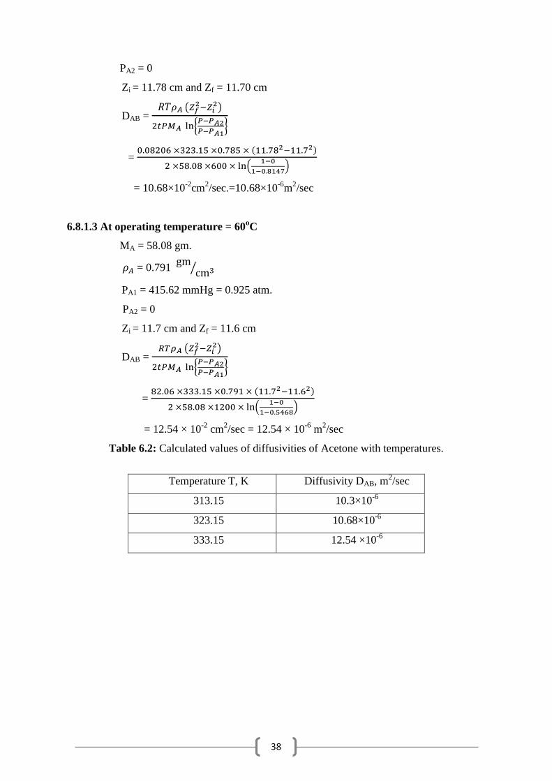
PA2 = 0

Zi = 11.78 cm and Zf = 11.70 cm

DAB = (

)

{

}

= ( )

(

)

= 10.68×10-2

cm2/sec.=10.68×10

-6m

2/sec

6.8.1.3 At operating temperature = 60oC

MA = 58.08 gm.

= 0.791

⁄

PA1 = 415.62 mmHg = 0.925 atm.

PA2 = 0

Zi = 11.7 cm and Zf = 11.6 cm

DAB = (

)

{

}

= ( )

(

)

= 12.54 × 10-2

cm2/sec = 12.54 × 10

-6 m

2/sec

Table 6.2: Calculated values of diffusivities of Acetone with temperatures.

Temperature T, K Diffusivity DAB, m2/sec

313.15 10.3×10-6

323.15 10.68×10-6

333.15 12.54 ×10-6

39

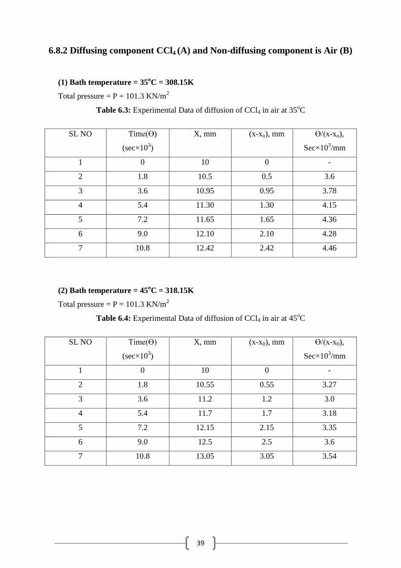
6.8.2 Diffusing component CCl4 (A) and Non-diffusing component is Air (B)

(1) Bath temperature = 35oC = 308.15K

Total pressure = P = 101.3 KN/m2

Table 6.3: Experimental Data of diffusion of CCl4 in air at 35oC

SL NO Time(ϴ)

(sec×103)

X, mm (x-xo), mm ϴ/(x-xo),

Sec×103/mm

1 0 10 0 -

2 1.8 10.5 0.5 3.6

3 3.6 10.95 0.95 3.78

4 5.4 11.30 1.30 4.15

5 7.2 11.65 1.65 4.36

6 9.0 12.10 2.10 4.28

7 10.8 12.42 2.42 4.46

(2) Bath temperature = 45oC = 318.15K

Total pressure = P = 101.3 KN/m2

Table 6.4: Experimental Data of diffusion of CCl4 in air at 45oC

SL NO Time(ϴ)

(sec×103)

X, mm (x-x0), mm ϴ/(x-x0),

Sec×103/mm

1 0 10 0 -

2 1.8 10.55 0.55 3.27

3 3.6 11.2 1.2 3.0

4 5.4 11.7 1.7 3.18

5 7.2 12.15 2.15 3.35

6 9.0 12.5 2.5 3.6

7 10.8 13.05 3.05 3.54

40

(3) Bath temperature = 55oC = 328.15K

Total pressure = P = 101.3 KN/m2

Table 6.5: Experimental Data of diffusion of CCl4 in air at 55oC

SL NO Time(ϴ)

(sec×103)

X, mm (x-xo), mm ϴ/(x-xo),

Sec×103/mm

1 0 10 0 -

2 1.8 11.2 1.2 1.5

3 3.6 12.0 2.0 1.8

4 5.4 12.95 2.95 1.83

5 7.2 13.8 3.8 1.895

6 9.0 14.55 4.55 1.978

7 10.8 15.45 5.45 1.982

6.8.2.1 Sample calculation

Vapour pressure of CCl4 can be obtained from the equation 6.23

*

+

Where T is in K and VP in Pa.

For CCl4

C1=78.441, C2= -6128.1, C3= -8.5766, C4=6.8465×10-6

, C5=2

With these values of constants the vapour pressure of CCl4 at 308.15 K is

*

( ) +KPa

= 23.14 KPa = 23.14 KN/m2

41

Fig: 6.2 Plot of (X-Xo) vs. ϴ/(X-Xo) at 308.15 K for CCl4

This graph yields a slope 0.4453

Least square equation of this line is

y= mx+C

i.e. y=0.4453x+3.443 and R² = 0.8723

From the graph, slope, s = 0.4453 sec×103/mm

2 = 4.453×10

8 sec/m

2

Total pressure= 101.3 KN/m2

Kilogram molecular volume of a gas = 22.4 m2 at 273.15 K

Total concentration =

0.04 Kmol/m

3

Molecular weight of CCl4=MA=154 Kg/mol

CA=concentration of CCl4= ( )

( ) = 9.14×10

-3 Kmol/m

3

Density of CCl4 = ρ1 = 1540 Kg/m3

Kmol/m

3

( ( ) )

( )

= 0.031Kmol/m

3

(

)

(

)

= 0.035 Kmol/m3

Now,

= 1.07×10

-6 m

2/sec at 35

oC

y = 0.4453x + 3.443 R² = 0.8723

0

1

2

3

4

5

0 0.5 1 1.5 2 2.5 3

ϴ/(

x-x

o)

x-xo

y

y

Linear (y)

42

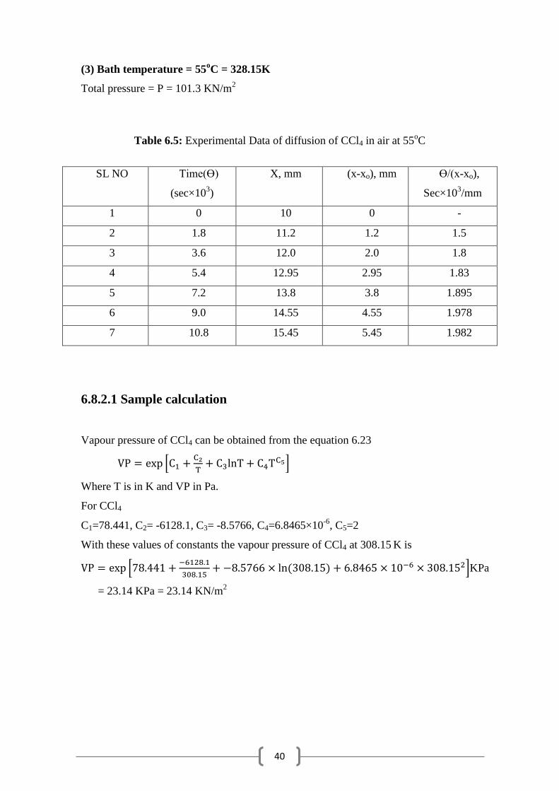
Fig: 6.3 Plot of (X-Xo) vs. ϴ/(X-Xo) at 318.15 K for CCl4

Fig: 6.4 Plot of (X-Xo) vs. ϴ/(X-Xo) at 328.15 K for CCl4

y = 01832x + 2.9829 R² = 0.5442

0

0.5

1

1.5

2

2.5

3

3.5

4

0 1 2 3 4

ϴ/(

x-x

o)

(x-xo)

y

y

Linear (y)

y = 0.1009x + 1.4955 R² = 0.8093

0

0.5

1

1.5

2

2.5

0 1 2 3 4 5 6

ϴ/(

x-x

o)

(x-xo)

y

y

Linear (y)

43

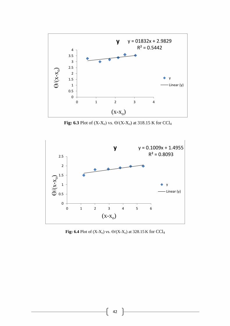
Table 6.6: Calculated values of diffusivities of CCl4 with temperatures.

Temperature T, K Diffusivity DAB, m2/sec DAB×P

308.15 8.87×10-6

0.898531

318.15 8.986×10-6

0.9102818

328.15 9.16×10-6

0.927908

Fig:6.5 Temperature vs. D×P on a log-log graph for CCl4

The equation from this graph is

D= 1×10-25

T9.65

/ P

From Gilliland‟s correlation,

For temperature = 308.15 K √ [

]

(

⁄

⁄ )

= √ (

)

( )

= 8.49 ×10-2

cm2/sec

=8.49×10-6

m2/sec

Similarly,

For T=318.15 K D = 8.68×10-6

m2/sec

For T=328.15 K D = 8.95×10-6

m2/sec

y = 1E-25x9.65

R² = 0.9272

0.0001

0.001

0.01

0.1

1

100 1000Dif

fusu

vit

y×

Pre

ssu

re

Temperature, K

44

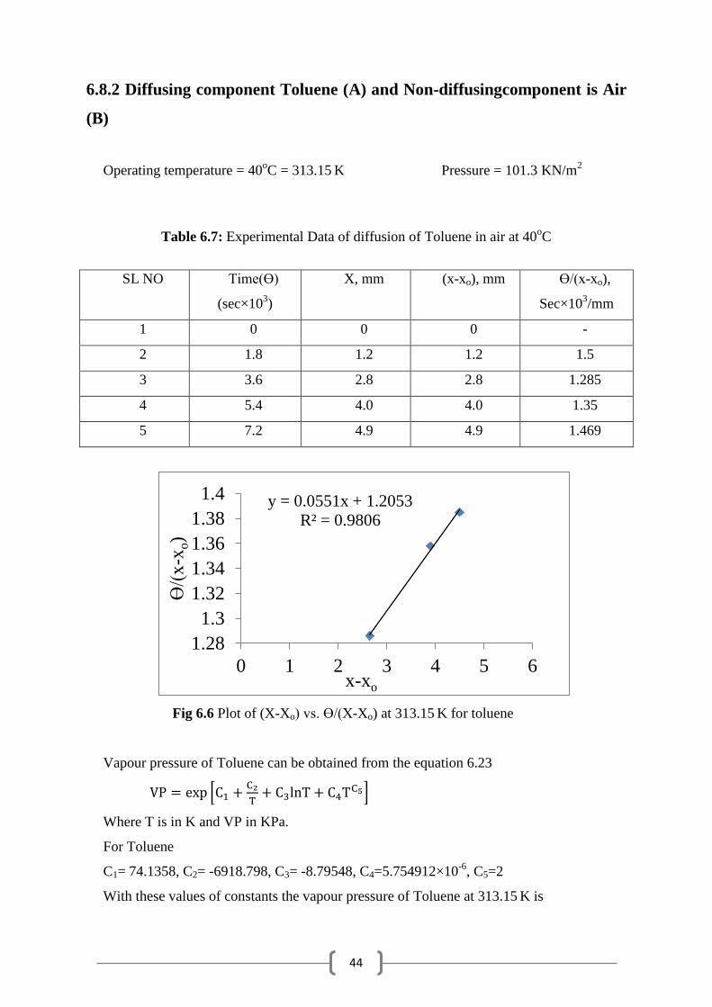
6.8.2 Diffusing component Toluene (A) and Non-diffusingcomponent is Air

(B)

Operating temperature = 40oC = 313.15

K Pressure = 101.3 KN/m

2

Table 6.7: Experimental Data of diffusion of Toluene in air at 40oC

SL NO Time(ϴ)

(sec×103)

X, mm (x-xo), mm ϴ/(x-xo),

Sec×103/mm

1 0 0 0 -

2 1.8 1.2 1.2 1.5

3 3.6 2.8 2.8 1.285

4 5.4 4.0 4.0 1.35

5 7.2 4.9 4.9 1.469

Fig 6.6 Plot of (X-Xo) vs. ϴ/(X-Xo) at 313.15 K for toluene

Vapour pressure of Toluene can be obtained from the equation 6.23

*

+

Where T is in K and VP in KPa.

For Toluene

C1= 74.1358, C2= -6918.798, C3= -8.79548, C4=5.754912×10-6

, C5=2

With these values of constants the vapour pressure of Toluene at 313.15 K is

y = 0.0551x + 1.2053

R² = 0.9806

1.28

1.3

1.32

1.34

1.36

1.38

1.4

0 1 2 3 4 5 6

ϴ/(

x-x

o)

x-xo

45

*

( ) +

= 7.895 KPa

Fig 6.5 yields a slope 0.0551

Least square equation of this line is

y= mx+C

i.e. y= 0.0551x + 1.2053 and R² = 0.9806

From the graph, slope, s = 0.0551 sec×103/mm

2 = 0.551×10

8 sec/m

2

Total pressure= 101.3 KN/m2

Kilogram molecular volume of a gas = 22.4 m2 at 273.15

oK

Total concentration =

0.038 Kmol/m

3

Molecular weight of Toluene = MA = 92 Kg/mol

CA=concentration of CCl4= CA ( )

( ) = 2.96×10

-3 Kmol/m

3

Density of Toluene = ρ1 = 866.9 Kg/m3

0.038 Kmol/m

3

( ( ) )

( )

= 0.035 Kmol/m

3

(

)

(

)

= 0.0365 Kmol/m3

Now,

= 8.15×10

-6 m

2/sec at 40

oC

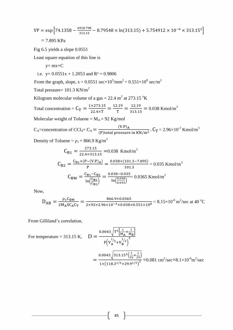
From Gilliland‟s correlation,

For temperature = 313.15 K, D √ [

]

(

⁄

⁄ )

√ (

)

( ) =0.081 cm

2/sec=8.1×10

-6m

2/sec

46

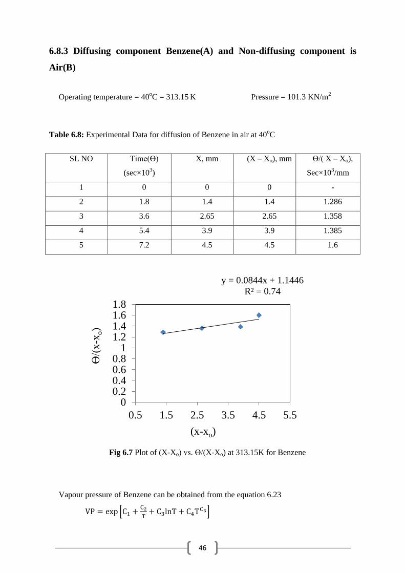
6.8.3 Diffusing component Benzene(A) and Non-diffusing component is

Air(B)

Operating temperature = 40oC = 313.15

K Pressure = 101.3 KN/m

2

Table 6.8: Experimental Data for diffusion of Benzene in air at 40oC

SL NO Time(ϴ)

(sec×103)

X, mm (X – Xo), mm ϴ/( X – Xo),

Sec×103/mm

1 0 0 0 -

2 1.8 1.4 1.4 1.286

3 3.6 2.65 2.65 1.358

4 5.4 3.9 3.9 1.385

5 7.2 4.5 4.5 1.6

Fig 6.7 Plot of (X-Xo) vs. ϴ/(X-Xo) at 313.15K for Benzene

Vapour pressure of Benzene can be obtained from the equation 6.23

*

+

y = 0.0844x + 1.1446

R² = 0.74

00.20.40.60.8

11.21.41.61.8

0.5 1.5 2.5 3.5 4.5 5.5

ϴ/(

x-x

o)

(x-xo)

47

Where T is in K and VP in KPa.

For Benzene

C1= 71.10718, C2= -6281.04, C3= -8.433613, C4=6.1984×10-6

, C5=2

With these values of constants the vapour pressure of Toluene at 313.15 K is

*

( ) +

= 24.34 KPa

Fig 6.5 yields a slope 0.0844

Least square equation of this line is

y= mx+C

i.e. y= 0.0844x + 1.1446 and R² = 0.74

From the graph, slope, s = 0.0844 sec×103/mm

2 = 0.844×10

8 sec/m

2

Total pressure= 101.3 KN/m2

Kilogram molecular volume of a gas = 22.4 m2 at 273.15 K

Total concentration =

0.038 Kmol/m

3

Molecular weight of Toluene = MA = 78 Kg/mol

CA=concentration of Benzene= CA ( )

( ) = 6.13×10

-3

Kmol/m3

Density of Benzene = ρ1 = 876.5 Kg/m3

0.038 Kmol/m

3

( ( ) )

( )

= 0.0288 Kmol/m

3

(

)

(

)

= 0.033 Kmol/m3

Now,

= 8.53×10-6

m2/sec at 40

oC

48

From Gilliland‟s correlation,

For temperature = 313.15 K, D √ [

]

(

⁄

⁄ )

√ (

)

( )

= 0.084 cm2/sec

= 8.4×10-6

m2/sec

6.9 Result

The binary diffusion coefficients of different solvents acetone, carbon tetrachloride, benzene

and toluene were determined and listed below.

Table 6.9 Experimental values of diffusional coefficients of some organic solvents

System Temperature(oC) Diffusivity(m

2/sec)

Air-Acetone

40 10.3×10-6

50 10.68×10-6

60 12.54 ×10-6

Air-CCl4

35 8.87×10-6

45 8.986×10-6

55 9.16×10-6

Air-Benzene 40 8.53×10-6

Air-Toluene 40 8.15×10-6

49

CHAPTER 7

Conclusion

7.1 Conclusion

This project work highlights the following facts:

(a) Binary diffusion coefficients of some industrially important organic solvents in air (a case

of diffusion of A through stagnant non-diffusing B) are effectively measured at widely

different temperatures and at atmospheric pressure in a Stefan tube set up. The data shows

that diffusivity varies considerably with temperature (directly proportional) and inversely

varies with pressure consistently for all the cases.

(b) Similarly, in case of spherical geometry (naphthalene balls) the average diffusivity is

found to be 3.43×10-7

m2/sec whereas for cylindrical geometry (camphor pellets) the

diffusivity value stands at 3.8×10-7

m2/sec. This indicates that it takes longer to diffuse from a

cylindrical shaped particle as compared to that in a spherical particle.

7.2 Future works

The present work can be extended to carry out further research in the following area:

(a) Systematic investigation on hydrocarbon systems to carry out binary diffusion studies

followed by multi-component assessment to calculate overall mass transfer coefficients

which would eventually be helpful in designing mass transfer equipments like distillation

(equimolar counter-current diffusion) and absorption columns/strippers (diffusion of A

through stagnant non-diffusing B).

(b) Liquid-liquid diffusion and/or gas-gas diffusion can also be extensively studied

fundamental to important unit operations.

(c) This study can particularly be useful in processed food packaging industries for controlled

assessment of diffusion of nutrients, aroma etc. for maintaining global standards (aesthetics

as well as nutrition wise).

(d) Diffusion studies (Knudsen and Surface diffusion) can be extended to heterogeneous gas-

solid catalytic reactions (particularly for catalysts with varying geometries) to understand the

mechanism further

50

REFERENCES

[1] Warren L. McCabe, Julian C. Smith, Peter Harriott, “Unit operations of chemical

engineering ”,McGraw-Hill 7th

edition,17,p.527-564 (2010)

[2] Robert E. Treybal, “Mass-Transfer operations-Diffusion”,ed-2nd

ch2,p21-93

[3] Binay K. Dutta,” Principle of Mass-Transfer and separation process-molecular diffusion”,

edition-5th

, 2013,p-11-42.

[4] F. Curtiss and R. B. Bird, “Multicomponent diffusion,” Ind. Eng. Chem. Res. 38, 2515

(1999)

[5] Bird, R. B., W. E. Stewart, and E. N. Lightfoot: “Transport phenomena,” Wiley, New

York, 1960.

[6] Arnold, J. H., “Studies in Diffusion: III Unsteady-State Vaporization and Adsorption.”

Trans. AIChE. 1944, 40,p 361.

[7] Slattery C. John, Bird Byron R., “Calculation of the diffusion coefficient of dilute gases”

AIChE. J., 1985,4,p 140-145.

[8] Hayduck, W., and H. Laudie: AIChE. J., 20, 611, 1974

[9] Hiss, T. G., and E. L. Cussler: AIChE J., 19, 698, 1973

[10] Jost, W,: ”Diffusion in solids, liquids and gases,” Academic, New york, 1960

[11] Newman, A. B.: Trans. AIChE j., 27, 203, 310,1931

[12] R.Van der Vaart, C. Huiskes, H. Bosch, T. Reith, Principle of diffusion (2000) 214.

[13] Hines, A.L., and R.N.Maddox, Mass transfer –Fundamentals and applications, Prentice

Hall, 1985.

[14] Perry‟s Chemical Engineers‟ Handbook, 7th

edition, McGraw-Hill, New york, 1997

[15] Skelland, A.H.P., diffusional mass transfer, john Wiley, New York, 1974

51

[16] Benitez, J., Principle and Modern applications of mass transfer, Wiley Interscience, New

York, 2002.

[17] Sherwood, T.K., R.L. Pigford, and C.R. Reid, Mass Transfer, McGraw Hill, New York,

1975.